nasa cr-132450 comoc: three-dimensional boundary region ... · nasa cr-132450 4. title and subtitle...
TRANSCRIPT

NASA C R - 1 3 2 4 5 04. Title and Subtitle
C O M O C : T h r e e - D i m e n s i o n a lBoundary Region Var ian t ;
Theore t i ca l M a n u a l " and U s e r ' s Gu ide' 7. Author(s)
A . J . Baker & S . W . Z e l a z n y
Bel l A e r o s p a c e CompanyP . O . Box OneBuf fa lo , New Y o r k 14240
12. Sponsoring Agency Nome and Address .
Nat iona l A e r o n a u t i c s and S p a c e Adm.W a s h i n g t o n , D . C . 20546
3. Recipient's Co to log No.
5. Report Dote
May 19746- Performing Organization Code
8- Performing Organization Report No.
D 9 1 9 2 - 9 5 0 0 0 210. Work Unit No.
"11. Contract or Grant No.
NAS1-1121413. Type of Report and Period Covered
Con t rac to r Repor t
14. Sponsoring Agency Code
15. Supplementary Notes
16. AbstractThe ThreerDimensional Boundary Region Variant of the COMOC computer
program system solves the three-dimensional boundary region equations fora viscous, heat conducting, m u l t i p l e species, compressible fluid i n c l u d i n gcombustion, The governing partial differential equations are solved inphysical varia-bles. The flow may be subsonic or supersonic, laminar and/orturbulent, and may contain up to nine or more distinct species in frozencomposition or undergoing e q u i l i b r i u m chemical reaction for a hydrogen/oxygen/air system. The program is equally a p p l i c a b l e to computations intwo- and three-dimensional boundary layer flows. COMOC is based upon afinite element solution algorithm for the partial differential equationsystems. It employs a finite difference integration algorithm procedureto solve the resultant systems of first-order, ordinary, differential equa-tions. Boundary condition constraints on the normal flux and tangentialdistribution of each dependent variable are user-specifiable on arbitrarilydisjoint segments of the solution domain closure. The solutions for eachdependent variable, and all computed parameters, are established at nodepoints lying on a specifiably non-regular computational lattice. The nu-merical solution establishes three-dimensional distributions of the threescalar velocity components, enthalpy, temperature, density, viscosity, anda p p l i c a b l e species mass fractions. Variable Prandtl number and speciesdiffusion coefficient distributions may be u t i l i z e d . This report documentsthe theoretical and mechanical structure of the computer program, and pre-sents guidance on adaptation of the code to solution of a particular prob-lem. Sample solutions are discussed for several problems, especially withrespect to solution accuracy and speed as a function of parameters undercontrol of the user. Construction of input data decks for sample problemsis discussed.
17. Key Words (S> lee ted by Author(s))
Numer ica l So lu t ionThree- D imens iona l F lowFini te E lement A l g o r i t h mC o m p r e s s i b l e , Turbu len tEqu i l ib r ium R e a c t i n a
9. Security Closiif. (of this report)
U n c l a s s i f i e d
18. Distribution Statement
For U . S . Government A g e n c i e sand their Con t rac to r s only
20. Security Classif. (of this page)
Uncl as si f ied
21. No. of Poges
73
22. Price*
•For sale by the Clearinghouse for Federal Scientific and Technical Information, Springfield, Virginia 22151-
https://ntrs.nasa.gov/search.jsp?R=19750024312 2018-11-19T13:22:04+00:00Z

0page

TABLE OF CONTENTS
Page
SUMMARY . . . . . . . . . . . 1
INTRODUCTION & USER GUIDELINES 2
FINITE ELEMENT SOLUTION ALGORITHM FOR THE THREE-DIMENSIONAL BOUNDARY REGION EQUATIONS 12
The Three-Dimensional Boundary Region Equations . . 12
Fin i t e Element Solution Algorithm ... 15
THE THREE-DIMENSIONAL BOUNDARY REGION VARIANT OF COMOC . 19i '
Finite Element Matrix Generation .20
Ordinary Differential Equation System IntegrationAlgorithm 25
Continuity Equation Solver 27
Computation of E q u i l i b r i u m Composition and Thermo-dynamic Properties of Hydrogen/Oxygen/Air Mixtures 28
ILLUSTRATIVE SOLUTIONS . . . . . . . . . 32
Constant Density Flows 32
Compressible Flow Fields 40
DATA DECK PREPARATION 59
CONCLUDING REMARKS . . . 65
REFERENCES 66
APPENDIX A ' . . . 68
APPENDIX B : 71

ILLUSTRATIONS
FIG. PAGE
1 COMOC Macro-Structure 42 I l l u s t r a t i v e F i n i t e Element Discretization . . . . 73 Intrinsic F i n i t e Element Domains for Simplex
Approximation Functions 204 Finite Element Discretization for Two-Dimen sional
Boundary Layer Flow 335 Computed Velocity Distributions, M = 0.272,
Rex = 0.63(7)/m 346 Computed Skin Friction and Boundary Layer Thickness,
M = 0.272, Rex - 0.63(7)/m . 357 Computed Solution Accuracy and Convergence,
M = 0.272, Rex = 0.63(7)/m 358 Integration Step-Size Distribution, M = 0.272,
Rex = 0.63(7)/m 379 Cross-Section of a Natural Stream Showing Measured
Isovels, [Ref. 16] . 3710 F i n i t e Element Discretization of Stream Cross-
Section 3711 Predicted Mass Fraction Contours at 9.6 m Down-
stream .of Injection, Three Diffusion Models ... 3912 Predicted Mass Fraction Contours at 9.6 m Down-
stream of Interface Injection 4013 Computed Supersonic Boundary Layer Parameters,
M = 5, Rex = .83(5)/m, 3 = 0.5. . • 4214 Computed Supersonic Boundary Layer Velocity, M = 5,
Rex = .83(5)/m, 3 = 0.5 4315 Integration Step Size Distribution, M = 5,
Rex = .83(5)/m, 3 = 0.5 4516 Computed Boundary Layer Velocity Profiles, M = 5,
Rex = .83(5)/m, 6 = 0.5 4617 Three-Dimensional Flow F i e l d Downstream of
Transverse Injection from Discrete Orifices ... 4718 F i n i t e Element Discretion of Symmetric Half-Space
of Single-Jet Injection Geometry 4819 Computed Hydrogen Mass Fraction and Experimental
Data for Single-Jet, qr = 1.0, X]/D = 60 . . . . 5020 Computed Single-Jet Hydrogen Mass Fraction
Distribution at X]/D = 60, qr = 1.0 5121 Isometric View of L o n g i t u d i n a l Velocity Surface for
Single-Jet Configuration, X]/D =30 5222 Computed Single-Jet Hydrogen Mass Fraction
D i s t r i b u t i o n at XI/D = 120, q^ = 1.0 5223 Computed Single-Jet L o n g i t u d i n a l Velocity
Distribution at x-j/D = 120, qr = 1.0 5324 Computed Multijet Hydrogen Mass Fraction
D i s t r i b u t i o n at x,/D = 60, qr = 1.0 53
i v

FIG. • PAGE
25 Computed Multijet Hydrogen Mass FractionDistribution at X]/D = 120, qr = 1.0 54
26 Computed Mass Fraction Contours and ExperimentalData for Multijet, x-|/D = 120, qr = 1 .0 . . . . . 54
27 Prediction for Multijet Virtual Source, qr = 1.0 . . 5628 Prediction for Multijet Virtual Source with
E q u i l i b r i u m Reaction, qr = I'-O 58
TABLES
NUMBER PAGE
1. Coefficients in Generalized Differential Equation . 162. General Boundary Condition Statement 173. I m p l i c i t Definition of Simplex Natural Coordinate
Functions. 214. Integrals of Natural Coordinate Function Products
Over Finite Element Domains 215. Standard Finite .Element Matrix Forms for Simplex
' Functionals in One- and Two-Dimensional Space . . 236. Coefficients in Integration Algorithm for Two, One-
Step, Three-Stage Methods 277. Species Identification for Reacting Hydrogen/
Oxygen/Air Systems 308. Parameters in Pollutant Dispersion Study 399. Data Deck Changes to Produce V i r t u a l Source
Simulation 64

COMOC: THREE DIMENSIONAL BOUNDARY REGION VARIANT
THEORETICAL MANUAL AND USER'S GUIDE
By
A. J . Baker & S. W. Z e l a z n y
Bell A e r o s p a c e Company
.SUMMARY
.The Three-Dimensional Boundary Region Variant of the COMOCcomputer program system solves the three-dimensional boundaryregion equations for flow of a viscous, heat conducting, m u l t i -ple species, compressible fluid including combustion. The gov-erning partial differential equations are solved in physicalvariables, and allow complete two-dimensional diffusion in theplane transverse to the predominant direction of flow. The flowfield may be external or confined, subsonic or supersonic, lam-inar and/or turbulent, and may contain up to nine or more dis-tinct species in frozen composition or undergoing e q u i l i b r i u mchemical reaction for a hydrogen/oxygen/air system. The programis equally a p p l i c a b l e to computations in two- and three-dimen-sional boundary layer flows wherein diffusion in only one direc-tion is important.
The COMOC computer program is based upon a finite elementsolution algorithm for the e l l i p t i c partial differential opera-tor in the parent equation system. It employs an e x p l i c i t finitedifference integration procedure to solve the resultant systemsof first-order, ordinary differential equations. Boundary con-dition constraints on the normal flux and tangential distributionof each dependent v a r i a b l e are user-specifiable on arbitrarilydisjoint segments of the solution domain closure. The solutionsfor each dependent variable, and all computed parameters, areestablished at node points lying on a specifiably non-regularcomputational lattice formed by plane triangulation of the solu-tion domain. The numerical solution establishes the completethree-dimensional distributions of the three scalar velocitycomponents, enthalpy, temperature, density, viscosity, and alla p p l i c a b l e species mass fractions, as well as various integralflow parameters. V a r i a b l e Pr.andtl number and species diffusioncoefficient distributions may be u t i l i z e d . I n i t i a l d i s t r i b u t i o n sof all dependent variables may be arbitrarily specified.
This report documents the theoretical and mechanicalstructure of the computer program, and presents detailed guidanceon adaptation of the code to solution of a particular problem.
Sample solutions are discussed for several problems, especiallywith respect to solution accuracy and speed as a function of pa-rameters under control of the user. Construction of the inputdata decks for sample problems is discussed. A programmer'smanual has been separately p u b l i s h e d [Ref. 1. ].
INTRODUCTION AND USER GUIDELINES
The finite element methodology for numerical solution ofinitial-boundary value problems in continuum mechanics is under-going an explosive rate of growth. Formerly .considered to beconstrained to solution of problems in structural analysis, orother l i n e a r field problems wherein an e q u i v a l e n t extremum prin-c i p l e exists, the theoretical support is now sufficiently gen-eralized to render the method directly a p p l i c a b l e to e x p l i c i t l ynonlinear problems, i n c l u d i n g the Navier-Stokes equations [Ref.2-4]. The COMOC computer program system is being developed totransmit this rapid theoretical progress (often couched in in-tricate mathematical formalism) into a v i a b l e and versatile nu-merical solution capability. As such, it must be a p p l i c a b l e todiverse and complex problems in computational continuum mechanicsw h i l e requiring m i n i m a l mathematical prowess on the part of theuser. On the way to generation of this general purpose concept,several Variants of COMOC have been developed for specific prob-lem classes i n c l u d i n g transient thermal analysis [Ref. 5] andthe two-dimensional Navier Stokes equations [Ref. 6]. This re-port documents the developed Three-Dimensional Boundary Region(3DBR) Variant of COMOC, and describes its a p p l i c a b i l i t y to awide range of practical two- and three-dimensional flow problems.
The 3DBR Variant of COMOC solves the three-dimensionalboundary region equations for flow of a viscous, heat conducting,m u l t i p l e - s p e c i e s , compressible f l u i d i n c l u d i n g combustion. Thegoverning partial differential equation system, developed in rec-tangular Cartesian coordinates from the parabolic Navier-Stokesequations, allows complete diffusion in the plane perpendicularto the uniformly d i s c e r n i b l e predominant flow direction. Theflow may be external or confined, subsonic or supersonic, l a m i n a rand/or turbulent, and can contain up to nine or more distinctspecies in frozen composition or undergoing e q u i l i b r i u m chemicalreaction for a hydrogen/oxygen/air system. The finite elementsolution procedure marches the discretized equivalent of thegoverning equation system in the direction p a r a l l e l to the pre-dominant flow. It numerically establishes the complete three-dimensional distributions of the three scalar velocity components,enthalpy, temperature, density, viscosity, and all a p p l i c a b l especies mass fractions, as well as various integral flow param-eters. No restrictions or s i m p l i f y i n g assumptions are made for
the Prandtl number, and i n d i v i d u a l species diffusion coefficientsare treated as v a r i a b l e parameters. I n i t i a l d i s t r i b u t i o n s of alldependent variables may be arbitrarily specified. Boundary con-dition constraints on the normal flux and tangential distributionof each dependent v a r i a b l e are user-specifiable on arbitrarilydisjoint segments of the solution domain closure. The solutionsfor each dependent v a r i a b l e , and all computed parameters, are es-tablished at node points lying on a specifiably non-regular com-putational lattice formed by plane triangulation of the solutiondomain.
All Variants of the COMOC system are b u i l t upon the macro-structure i11ustrated in Fig. 1. The Main executive routine al-locates core, using a v a r i a b l e d i m e n s i o n i n g scheme, based uponthe total degrees of freedom of th.e problem. The size of thelargest problem that can be solved is thus limited (only) by thecore size of the computer in use. The precise mix between numberof dependent variables (and parameters), and fineness of the dis-cretization, is user-speci f i.abl e and widely variable. The Inputmodule serves its standard .function for all dependent variable,parameter, and geometric coordinate arrays. The Discretizationmpdule forms the finite element discretization of the solutiondomain, and'evaluates all required finite element non-standardmatrices and standard-matrix m u l t i p l i e r s . The I n i t i a l i z a t i o nmodule computes the remaining i n i t i a l parametric data requiredto start the solution. The Integration Module constitutes theprimary execution sequence of problem solution. It is based uponan integration algorithm for the column vector of unknowns of thesolution, for which the discretized description is i n i t i a l - v a l u e d ,C a l l s to auxiliary routines for parameter e v a l u a t i o n , e.g. vis-cosity, Prandtl number, source terms, combustion parameters, etc.as specified functions of dependent and/or independent variablesare governed by the Integration Module. The user has consider-able latitude to adapt COMOC to the specifics of his particularproblem at this point, by directly inserting easily written sub-routines into COMOC to compute special forms of these parameters.The Output module is similarly addressed from the integrationsequence and serves its standard function via a h i g h l y automatedarray display algorithm. COMOC can execute distinct problems insequence and contains an automatic restart capability to continuesoluti ons.
The 3DBR -Variant of COMOC, as a direct consequence of theexpansive problem class to which it may be. addressed, is a fairlylarge and complex computer program. The vigor with which thepotential user of a computer code attacks preparation of a datadeck decreases exponentially (at least) with the thickness of theinstruction manual. It is the intent of this user's guide to,in a m i n i m u m amount, of space, present general g u i d e l i n e s for theuse of COMOC-, describe t.he rudiments of the differential equationsystem being solved, briefly expose the basic mathematics

INITIALIZATION
DISCRETIZATION
INTEGRATION
PARAMETEREVALUATION
YES
NO
©
NO-H C
YES•0
Figure 1. COMOC Macro-Structure

of the finite element algorithm and its numerical embodiment,and discuss sample solutions with respect to accuracy, solution,speed, and diversity. The standard test cases that accompanyCOMOC are discussed in terms of the physics of the solution aswell as the description of data deck preparation. A large efforthas been made to s i m p l i f y and streamline data preparation and torequire the user to specify an absolute m i n i m u m of non-physicalor non-engineering input. The basic program contains a m u l t i t u d eof options which could potentially '1ead to confusion on the partof the user. Most of these have been suppressed, particularlyin the output sub-program, with default instructions or values.The programmer's manual [Ref. 1] describes how they may bereturned to an operational status.
The following general g u i d e l i n e s w i l l assist the potentialuser on adapting 3DBR COMOC to a given problem.
Solution Domain Configuration
Most three-dimensional flow fields for w h i c h , 1) a predom-inant flow direction persists (i.e., no recirculation component),2) a prescribed pressure gradient can be established, and 3) noimbedded shocks occur, are amenable to analysis using 3DBR COMOC.This includes two- and three-dimensional boundary layer flows,certain two- and three-dimensional flows in environmental hydro-dynamics, and free-, slot-, and boundary-jet injection config-urations typical of combustors. Boundary conditions can be ap-p l i e d to the entire solution domain closure with local normalorthogonal to the direction of predominant flow. An i n i t i a l dis-tribution (i ncl udi ng zero) of all dependent variables is neededto start the solutic-n. However, a downstream outflow boundarycondition is specifically not required.
Variables and Parameters
The computational variables are the three scalar componentsof velocity, stagnation enthalpy, and mass fraction of all iden-tif i a b l e species. Perfect gas behavior is assumed. The present3DBR Variant solves the mainstream and one cross-plane velocitycomponent as a boundary v a l u e problem; it employs the continuityequation to establish the remaining cross-plane velocity componentThe program computes static temperature and density, and allthermophysical properties may be temperature and mass fractiondependent. Unless overridden by a user provided subroutine, vis-cosity is computed from Sutherland's law. The Prandtl and Schmidtnumbers may be variable. E q u i l i b r i u m combustion of arbitrarymixtures of hydrogen, oxygen, and air can be established i n c l u d i n glocal heat release and formation of NO. In the absence of d i l -uents, this capability provides e q u i l i b r i u m gas behavior for aircomputations i n c l u d i n g dissociation.

Di sereti zati on
The nature of the flows to which this Variant is a p p l i c a b l eyields the requirement for two-dimensional finite element dis-cretizations only. Since the continuity equation is employed tosolve for a transverse velocity component, it is advantageous tohave node columns oriented par a l l e l to that coordinate. This re-quirement for grid regularity has been b u i l t into an automaticdiscretizer for 3DBR COMOC. Considering flow in an axial cornerfor example, see Fig. 2, it might be desired to use a finer gridnear the w a l l s where larger dependent variable gradients wouldexist. The user need specify (only) the desired incrementalspacing between node columns and rows. The discretizer w i l l au-tomatically triangulate the domain on these node point coordinates,and prepare the required geometric input data. This discretizeris not directly a p p l i c a b l e to non-rectangular domains; however,3DBR COMOC can accept discretizations formed m a n u a l l y or fromother automated sources.
Boundary Conditions
Constraints can be imposed on the admissible behavior ofeach dependent variable and its normal flux, i.e., gradient, onall surfaces bounding the solution domain, see Fig. 2. Thesesurfaces may constitute actual physical boundaries of the problemor be strictly mathematical. As an example of the latter, em-ploying symmetry planes to enclose a solution domain is particu-larly advantageous in terms of computer execution time and userinput effort. The attendant v a n i s h i n g gradient constraint isthe automatic default v a l u e w i t h i n the finite element solutionalgorithm, and its use does not require generation of any phantomcells or special node h a n d l i n g . F i x i n g the normal gradient interms of the dependent v a r i a b l e is equally straightforward, andis useful for thermally porous w a l l s or a s l i p w a l l boundarycondition. Here again, no special cells or node h a n d l i n g isrequired on the part of the user.
Input Preparation
A concerted effort has been made to render i n p u t preparationm i n i m a l and in terms of p h y s i c a l l y meaningful variables and ex-pressions. However, should the solution to a dozen or more de-pendent v a r i a b l e s be sought, the i n p u t deck can become of sub-stantial size. The program accepts input in the Engl.ish systemof units; it outputs n o n - d i m e n s i o n a l i z i n g constants and solutionparameters in several systems, and provides detailed output ar-rays of computed non-dimensional dependent variables. The pro-gram executes under automatic error control and w i l l adjust inte-gration step-size to maintain an accurate and stable solution. Theonly user input required for this phase is the i n i t i a l and final

integration stations and the desired interval for output. Someadd i t i o n a l options exist that can speed execution for some cases[Ref. 1]. These parameters are defaulted to "best" values if notoverridden by the user.
//// = Boundary Condition Specification
Figure 2. Illustrative Finite Element Discretization
User-Written Subroutines
COMOC provides the user with considerable latitude forappending subroutines to perform specific parameter computationsIncluded in this category are pressure gradient, laminar and/orturbulent viscosity, and Prandtl and Schmidt numbers. In allcases, a skeletal subroutine is f i l l e d in by the user to i n c l u d ean equation or tabular data of the parametric dependence on anynumber of independent or dependent variables in any combination.These subroutines are always written in terms of physical vari-ables with dimensions consistent with the input data. Non-dimen-sional ization and c a l l i n g sequence are controlled internally,and the user can obtain complete arrays of these computationsfrom the output package.

Output
The 3DBR COMOC program contains a h i g h l y adaptive outputsubprogram. The user has considerable latitude in specifyingoutput arrangements, both dimensional and non-dimensional, fromthe input deck. The output routine is adapted to compute inte-gral flow parameters i n c l u d i n g wall shear, Stanton number, andm i x i n g efficiency. Data sets are automatically scaled and orderedto be geometrically s i m i l a r to the physical problem for all dis-cretizations, both regular and non-regular.
Computational Costs
The computer cost associated with generating a COMOC solutionto a given problem can be approximately estimated. CPU costs arebas.ically a function of the number of dependent variables in thesolution, the amount of output requested, out-of-core operationsassociated with restart and/or plot tape preparation^, and thethermodynamics of the solution. .The use of rather course discre-tizations is strongly recommended for i n i t i a l e v a l u a t i o n of anyproblem. Employing progressively finer discretizations w i l l gen-erally improve solution accuracy with a more-than-proportional in-crease in computational cost.
NOMENCLATURE
a boundary condition coefficient
A species; one-dimensional matrix; area
Ar argon
b coefficient
B species; two-dimensional matrix
c coefficient
CD specific heat
C species; three-dimensional matrix
C f skin friction
d differential
D determinant
f function of known argument
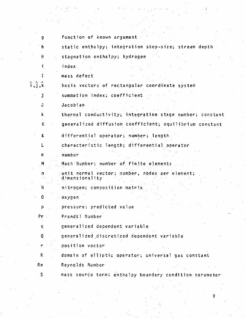
g function of known argument
h static enthalpy; integration step-size; stream depth
H stagnation enthalpy; hydrogen
i i ndex
I mass defect
i,j,k basis vectors of rectangular coordinate system
j summation index; coefficient
0 Jacobian
k thermal conductivity; integration stage number; constant
K generalized diffusion coefficient; e q u i l i b r i u m constant
1 differential operator; number; length
L characteristic length; differential operator
m number .
M , Mach Number; number of finite elements
n unit normal vector; number, nodes per element;• dimensional i ty . •
N nitrogen; composition matrix :
0 oxygen
p pressure; predicted value
Pr Prandtl Number
q generalized dependent variable
Q generalized discretized dependent variable
r p o s i t i o n v e c t o r
R domain of e l l i p t i c operator; universal gas constant
Re Reynolds Number . .
S mass source term; enthalpy boundary condition parameter

Sc Schmidt Number
T temperature
u,U velocity
W molecular weight
x. r.ectangular Cartesian coordinate system
X species mole fraction
Y species mass fraction
a direction cosi.ne
g coefficient; pressure gradient parameter
Y ratio of specific heats; turbulence intermittencyfactor
9R closure of solution domain
<5 boundary layer thickness
A increment
e kinematic eddy viscosity; basis vectors; integrationoarameter
K coefficient
X m u l t i p l i e r
£ non-dimensional length
y viscosity
p density
a integral kernel
T integral kernel; w a l l shear
4>, $ functional
X domain of i n i t i a l v a l u e operator
to turbulence damping factor
fi global solution domain
10
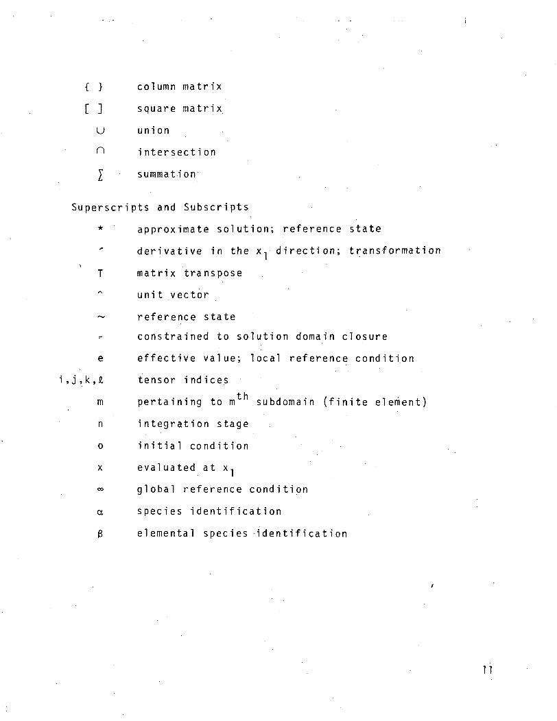
{ } column matrix
[] square matrix
U union
^ intersection
£ summation
Superscripts and Subscripts
* approximate solution; reference state
derivative in the x, direction; transformation•>!
T matrix transpose
unit vector
~ reference state
constrained to solution domain closure
e effective v a l u e ; local reference condition
i,j,k,£, tensor indices
m pertaining to m .subdomain (finite element)
n integration stage
o i n i t i a 1 c o n d i t i o n
x evaluated at x,
°° g l o b a l reference condition
a . species identification
B elemental species identification
11

FINITE ELEMENT SOLUTION ALGORITHM FOR THE THREE-DIMENSIONALBOUNDARY REGION EQUATIONS
The system of partial differential equations governing thethree-dimensional boundary region flow of a compressible f l u i dis obtained from the parabolic approximation to the full Navier-Stokes equations. The parabolic approximation, i.e., "parabolicNavier-Stokes equations," describe steady, three-dimensional flowswherein, 1) a predominant flow direction is uniformly discernible,2) in this direction (only), diffusion processes are n e g l i g i b l ecompared to convection, and 3) no disturbances are propagated up-stream antiparallel to this direction. The boundary region equa-tion system is obtained from parabolic Navier-Stokes with thesingle additional assumption that a known pressure distributionis superimposed upon the flow field. Conversely, the approxima-tion may be viewed as generalization of the three-dimensionalboundary layer equations to include diffusion processes in thecomplete two-dimensional plane of crossflow. Closure of thisequation system requires identification of constitutive behavior.By employing an eddy coefficient hypothesis, the time-averagedturbulent flow equations appear identical to the laminar flowequations. Hence, the finite element development assumes a gen-eralized transport coefficient description, distributed as lami-nar or turbulent at nodes of the discretization by the user.
The Three-Dimensional Boundary Region Equations
In three-dimensional space, spanned by a rectangular Carte-sian coordinate system, identify the velocity vector
/s. s*. /*.
u . = u, i + u £ j + u 3 k (1 )
For development of the differential equation system, assume thati is aligned p a r a l l e l to the predominant flow direction. Iden-tify a two-dimensional vector differential operator as
^ s\
( ),k = j(. ),2 + k( ),3 (2)
where the comma identifies the gradient operator. EmployingCartesian tensor notation, with summation over 2 and 3 for re-peated latin subscripts, the three-dimensional boundary regionequation system for a m u l t i p l e - s p e c i e s , compressible, reactingflow takes the form
0 1 \ i / \ / n \= (pu-),. +(pu 1), 1 (3)
12

ou Ya
pVi,i
PU1U3,1
Sc-Re
e
Y«
- PU.U'k
J'k
,' » 1
- Sa
- PM
- P>3
(4)
(5)
(6)
Re-Pr H,, " p U H '
pr
Sc-PrSc-Pr
'k 'k
(7)
The variables appearing in Eq. (3)-(7) are non-dimensionalizedwith respect to POO, U^, Cp^, TM, and a length constant L, andhave their usual interpretation in flu id mechanics. The Reynolds(Re), Prandtl (Pr), and Schmidt (Sc) numbers are defined withrespect to the effective diffusion coefficient, ye, in algebraiccombination with the laminar and turbul en't contri buti ons as, forexample
(8)Pr_Pr
In Eq. (8), y is the laminar viscosity, e is the kinematic eddyviscosity., and subscript T denotes a turbulent reference param-eter. The stagnation enthalpy is defined in terms of speciess t a t i c e n t h a l p i e s a s
H I haY( \ uk uk
The static enthalpy includes the heat of formation,species in its definition as
h" ,
'dT + ha
(9)
of the
(10)
13
An equation of state is required to close the system. Assumingperfect gas behavior for each species, from Dalton's law, obtain
pRTa Wa
(11)
where R is the universal gas constant and Wa is the molecularweight of the ct-th species.
E q u i l i b r i u m combustion of hydrogen/oxygen/air systems inthree-dimensional boundary region flow is operational in 3DBRCOMOC. The following reactions are assumed operative.
2H +
H +
0 4-
2H t
20 £
0 J
H2°
H2
°2
OH
20 «- 2ND (12)
The e q u i l i b r i u m composition ofdetermined by applying the Lawreaction defined in Eq . (12).of equilibrium rate constants,nA + mB -<- aC, are expressed inXa, as
the combustion by-products isof Mass Action [Ref. 7] to eachThis y i e l d s definition of a setK, w h i c h , for the simple reactionterms of species mole fraction,
K E [XA]n[XB]m(13)
Solution of Eq. (12) with (13), and coupled with conservation oftotal and elemental mass, yields an algebraic equation systemfor determination of the e q u i l i b r i u m composition of the system,of the form.
{const. } (14)
In Eq. (14), the elements of the matrix [N^] account for theparticular species mole fraction d i s t r i b u t i o n , {Xa}, containingthe gth elemental material, e.g., 0, H, and N.
14

Finite Element Solution Algorithm
The three-dimensional boundary region equation system,except' for global continuity, Eq. (3), is uniformly an i n i t i a l -boundary value problem of mathematical physics. Each of thepartial differential equations, Eq. (4)-(7), is a special caseof the general second-order, nonlinear partial differentialequati on
L(q) = K[K(q)q,.J + f(q,q,.,x.) - g(q,X) = 0 (15.)K ,k i i
•where q is a generalized dependent v a r i a b l e i d e n t i f i a b l e with"each computational dependent variable. In Eq. (15), f and g arespecified functions of their arguments, x 1S identified with X]for boundary region flows, and XT are the coordinates for whichsecond order derivatives exist in the lead term. The finiteelement solution algorithm is based upon the assumption thatL(q) is uniformly parabolic w i t h i n a bounded open domain ft, i.e.,the lead term in Eq. (15) is uniformly e l l i p t i c w i t h i n its domainR, with closure 3R, where
n = R x [Xo,x) (16)
and x £ X < °°- Table 1 lists the functions f and g, as wellas the appropriate parameters, for Eq. (15) identified with eachdependent v a r i a b l e .
For Eq. (15) uniformly p a r a b o l i c , unique'solutions for qare obtained pending specification of boundary constraints on3R and an i n i t i a l condition on RU8R. For the former, the gen-eral form relates the function and its normal derivative every-where on the closure, 3R, as
£(q) E a(1)q(xi,x) + a(2)Kq(x1,x),knk - a
(3) = 0(17)
In Eq . (17), the a'1' . ) are user-specified coefficients, seeTable 2, the superscript bar notation constrains x-j to 3R, andn|< is the local outward-pointing unit normal vector. For an i n i -tial distribution, assume given throughout RU3R x x
q(x.,x0) = qo(x.j) (18)
15

LU
m .1 — i
LU
CD
<4-
^
y
cr
o
crUJ
Q « -I-} •>>- 3 :c
3 13 3Q. Q. Q.
-i£•\
r \.
f\
•<~3
^
JQJ«(NJ
s_Q_ S_
1 0.
•1-3 ' '
3 Q. OJ 8oo s:+ i
:.*: :
a ** <ro **
Q. Q. Q.
I I I
<U 1 O 0} 0) \i-^L]C/) 3. — <|o
i i iO) O) O)a: oi o:
£5 *r~^>~ 3 31
5«* i
LO
-^•\
[ \
^£ •
8-
a
ixi aQJ JOJ
S_Q- S-
1 Q-0 0oo oo
1 1
1
•

TABLE 2
GENERAL BOUNDARY CONDITION STATEMENT
Boundary Conditions
No S l i p at Wall
Slip at WallMass Injection
Adiabatic WallSpecified Heat Flux
Temperature Dependent FluxSymmetry Condition
a<'>
1
+
0
0
0+
0
a< 2>
0111111
a < 3 >
0
0
+
0
+
+
0
+ User specified as non-zero to enforce desired condition level
Formation of the finite element solution is obtained byestablishing the algorithm for the equation system (15)-(18).Straightforward theoretical development is provided by using theM.e;t'hod of Weighted Residuals (MWR) formulated on a local basis.Since Eq. (15) is v a l i d throughout R, it is v a l i d withininterior subdomains, Rm, described by (x-j ,x)eRm
x [Xo>x)finite elements," wherein URm = R. Form an approximate
[Xo»x)» calledfor q within Rmseries solution of the form
,x) > bY expansion
disjointcalledsolution
i nto a
{0>(xi)}T{Q(x)}m (19)
'wherein the functionals (^(x-j) are members of a function set com'plete in Rm, and the unknown expansion coefficients, Qk(x)> rep-resent the x-dependent values of qjfj(x-j,x) at specificinterior to Rm and on the closure, 8Rm, called "nodes(19) is a scalar, and selection of the particular <j>^ is d i s t i n c t -ly specifiable [Ref. 8] and can be problem class dependent.
1ocati onsEquati on
To establish the values taken by the expansion coefficientsin Eq. (19), require that the local error in the approximate so-lution to both the differential equation, L'tqjfi) , and the boundarycondition statement, i(qjfj), for 8RmnaR, be rendered orthogonalto the space of the approximation functions. Employing an un-known algebraic m u l t i p l i e r , X, the resultant equation sets canbe combined as
{<t.(xi)}L(q*)dT -
m
xi))^(q*)da = 0
H3R
(20)
17

The number of equations (20) is i d e n t i c a l to the number of nodepoints of the finite element, Rm, i.e., the number of elements,n, in the column matrix, {Q(x)}m> Eq . (19).
Equation (20) forms the basic operation of the finiteelement solution. Establishment of the global solution algo-rithm, and determination of X, is accomplished by e v a l u a t i n gEq. (20) in each of the M finite elements of the discretizedsolution domain, and assembly of these M x n equations into aglobal matrix system u s i n g Boolean algebra. The rank of theglobal system is less than M x n by connectivity of the finiteelement domains as well as boundary condition constraints on 9Rwhere a (2), Eq. (17), vanishes identically. The lead term inEq. (15) can be rearranged, using the Green-Gauss Theorem, toyield
fWx^MKqJ^] dT . = K
n <\ nKm 9Km
|{+{x1)}.kKq;.k<lT (21)
Rm
For 9RO9Rm n o n v a n i s h i n g , Eq. (21), the corresponding segment ofthe closed surface integral w i l l cancel the boundary conditioncontribution, Eq. (20), by identifying Xa(2) with K of Eq. (15).The contributions to the closed surface integral, Eq. (21), where9Rmn9R = 0 can be made to vanish [Ref. 4]. Hence, combining Eq.(17)-(21), the g l o b a l l y assembled finite element solution algo-rithm for the representative partial differential equation systemdescription becomes
U
Rm Rm
- K l{*Ham1}q* - am
; {0} (22)
18
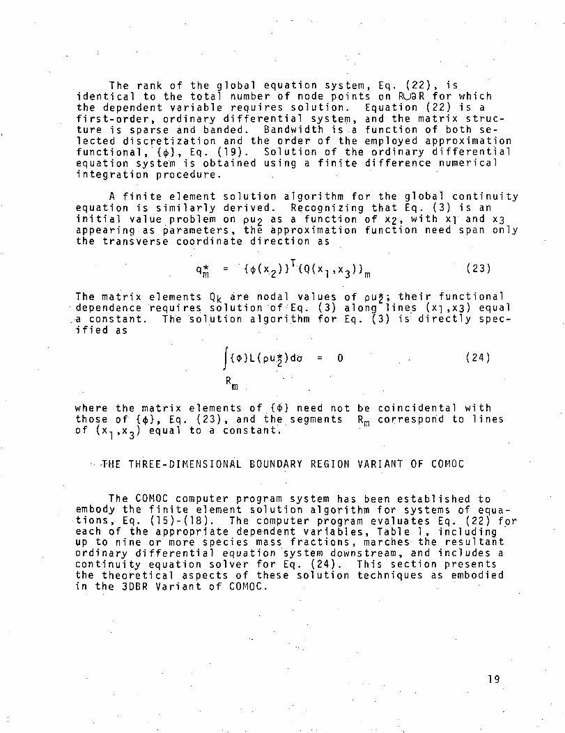
The rank of the global equation system, Eq. (22), isidentical to the total number of node points on RU8R for whichthe dependent variable requires solution. Equation (22) is afirst-order, ordinary differential system, and the matrix struc-ture is sparse and banded. Bandwidth is a function of both se-lected discretization and the order of the employed approximationfunctional ,{<(>}, Eq. (19). Solution of the ordinary differentialequation system is obtained using a finite difference numericalintegration procedure.
A finite element solution algorithm for the global continuityequation is similarly derived. Recognizing that Eq. (3) is ani n i t i a l value problem on pu£ as a function of xg, with xy and xsappearing as parameters, the approximation function need span onlythe transverse coordinate direction as
q*Hm 1 (23)
The matrix elements Q|< are nodal valuesdependence requires solution of Eq. (3)a constant. The solution algorithm forified as
of p u $; their functionalalong lines (x ] , x 3) equalEq. (3) is directly spec-
f{$}L(pu*)da = 0 (24)
wherethoseof
m .
the matrix elements of {$} need not be coincidental withof {<|>}, Eq . (23), and the segments R^ correspond to lines
equal to a constant.(x, ,x3)
-THE THREE-DIMENSIONAL BOUNDARY REGION VARIANT OF COMOC
The COMOC computer program system has been established toembody the finite element solution algorithm for systems of equa-tions, Eq. (15)-(18). The computer program evaluates Eq. (22) foreach of the appropriate dependent variables, Table 1, i n c l u d i n gup to nine or more species mass fractions, marches the resultantordinary differential equation system downstream, and includes acontinuity equation solver for Eq. (24). This section presentsthe theoretical aspects of these solution techniques as embodiedin the 3DBR Variant of COMOC.
19
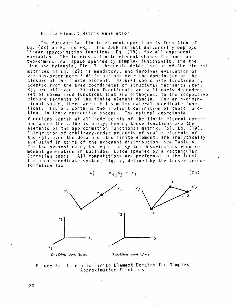
F i n i t e Element Matrix Generation
The fundamental finite element operation is formation ofEq. (22) on R^ and 3Rm. The 3DBR Variant universally employslinear approximation functions, Eq. (19), for all dependentvaria.bles. The i n t r i n s i c finite element shapes for one- andtwo-dimensional space spanned by simplex functionals, are thelin e and t r i a n g l e , Fig. 3. Accurate determination of the elementmatrices of Eq. (22) is mandatory, and i n v o l v e s evaluation ofvarious-order moment distributions over the domain and on theclosure of the finite element. Natural coordinate functionals,.adapted from the area coordinates of structural mechanics [Ref.8], are utilized. Simplex functionals are a linearly dependentset of normalized functions that are orthogonal to the respectiveclosure segments of the finite element domain. For an n-dimen-sional space, there are n + 1 simplex natural coordinate func-tions. Table 3 contains the i m p l i c i t definition of these func-tions in their respective spaces. The natural coordinatefunctions vanish at all node points of the finite element exceptone where the v a l u e is unity; hence, these functions are theelements of the approximation functional matrix, {<f>}, Eq. (19).Integration of arbitrary-order products of scalar elements ofthe {$}, over the domain of the finite element, are analyticallyevaluated in terms of the exponent d i s t r i b u t i o n , see Table 4.For the present case, the equation system descriptions requiremoment generation in Euclidean space spanned by a rectangularCartesian basis. All computations are performed in the local(primed) coordinate system, Fig. 3, defined by the tensor trans-formation law
xi aijX. + r. (25)
One-Dimensional Space Two-Dimensional Space
Figure 3. Intrinsic F i n i t e Element Domains for SimplexApproximation Functions
20

TABLE 3
IMPLICIT DEFINITION OF SIMPLEX NATURALCOORDINATE FUNCTIONS
D i m e n s i o n s
1
2
.Element
Line
Triangl e
Nodes
2
3
Natural Coord ina te De f i n i t i on
"; jj.r+ij . f_ i)" i i i "
1 2 3X l X l X l
1 2 3A f\ O *?
<
1 i J
f*i]
*2
UJ1 = (
1 "xlixj
>
TABLE 4
INTEGRALS OF NATURAL COORDINATE FUNCTIONPRODUCTS OVER FINITE ELEMENT DOMAINS
Dimens ions
1
2
In tegra ls*
C n , n 2 n , ! n 2 !1 A A rl rr ~ H — — — •J R .1 2 (n + n1 + n2) !
/• n, n 2 n 3 . . n 1 ! n 2 ! n 3 !
J P 1 ^2 3 (n + n, + n9 + n-,)!' K 1 c. O
* .D = Determinant of coefficient matrix defini-ng thenatural coordinate system, see Table 3.
n = Dimensionality of the finite element space
where n is the position vector to the origin of the primedcoordinate system, and the a-jj are the direction cosines of thecoordinate transformation. Tne integration kernels for two-dimensional space, Eq. (22), are
dt
da
dx2dx3
dx'
(26)
(27)
21

The first term in Eq. (22) is standard for all dependentvariables. Assuming the generalized diffusion coefficient isdistributed over the m'-'1 element as a dependent v a r i a b l e , obtain
K { < j > } , k K q * , k d T =
. Rm Rm
= K{K}T{B10}[B211S]{Q}m (28)
In Eq. (28) and the following, matrices with B prefixes arestandard two-dimensional forms defined in Table 5. For Eq . (22)identified with each dependent v a r i a b l e , f* and g* u n i v e r s a l l ycontain the nonlinear convection term and the i ni ti al -val ueoperator as dominant terms. The finite element e q u i v a l e n t forconvection is
Rm Rm
= [B200S] {p t r } m {B l l } T {Q} m (29)
where the e lemen ts of the vec to r , { p u ^ } , are nodal v a l u e s of thep lanar m a s s f l ux t rans fo rmed to the loca l coo rd ina te sys tems v ia
The i ni ti al - val ue operator, which comprises the mainstreamconvection term, s i m i l a r l y becomes
j {< i>H<|>}T {pUl } n i {L}T {Q} rJdT
Rm Rm
= •{PU1}J[B3000S]{Q}^ (31)
where the matrix elements of [B3000S].are column matrices, seeTable 5. The superscript prime exterior to a matrix denotes anordinary derivative.
22
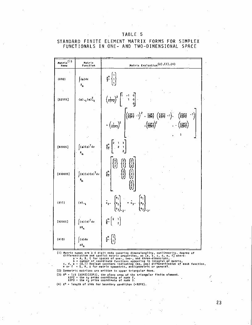
TABLE 5
STANDARD FINITE ELEMENT MATRIX FORMS FOR SIMPLEXFUNCTIONALS IN ONE- AND TWO-DIMENSIONAL SPACE
MatrixName '1*
MatrixFunction Matrix Eva luat1on ( 2 ) > ( 3 ) l ( 4 )
{810}
[B211SJ
J<*>dT
.{*>.k<*>!k
X3P3 ,\2
"y •X3P3 X3P3 X3P3 -1
X3P3\/
1
[B200S]
[B3000S] {»H<t>H<t>}dT
f6! f2!< 2 > h i12J U
li
{BID
[A200S]
{AID}
3R
({*}do
3R
(1) Matrix names are a 6 digit code covering dimensionality, nonllnearlty, degree ofdifferentiation and special matrix properties, as [a, b, c, d, e, f] where:
a '« A, B, C for spaces of one-, two-, and three-dimensions,b • number of coordinate functions appearing In Integral or matrix,
c, d, e = (0,1) Boolean counters indicating (no, yes) differentiation of each function,e or f = S, A, A for matrix symmetric, antisymmetric or general.
(2) Symmetric matrices are written in upper triangular form.(3) Ara = 1/2 (X2P2)(X3P3), the plane area of the triangular finite element.
X2P2 = the xz prime coordinate of node 2,X3P3 = the Xj prime coordinate of node 3.
(4) lm =• length of side for boundary condition (-X2P2).
23

Both momentum Eq. (5) and (6) contain contributions to f^stemming from a specified pressure distribution. For the m a i n ^stream momentum equation, a specified l o n g i t u d i n a l pressuregradient, p,-,, is assumed kpown; hence,
_i _ r n 1 ri\ ^ ( V \ / "3 O \, i Q T — i t 5 I U / p » i \ A i / . \ o L I
m
For. a lateral .pressure g rad ien t , ob ta in
{ 4 > } p , 3 d T =
Rm
{ B 1 0 H B l l } { P Z } r a ( 3 3 )
where the matrix elements of {PZ } are obta ined from the tensort rans fo rmat ion l a w , Eq . ( 2 5 ) , as
PZ, a. (34)
Each s p e c i e s cont inu i ty e q u a t i o n , E q . ( 4 ) , may have a sourceterm. A s s u m i n g the d is t r ibu t ion to l ie over the nodes of thed i s c r e t i z a t i o n , ob ta in
j{<|>}Sa dT [B200S]{Sa} (35)
m m
For non-constant Prandtl and Schmidt Numbers, the energy equationEq . (7), has two source terms. An integration using a Green-Gauss Theorem is appropriate for both; the generated surface in-tegrals vanish by pairs onon 3RmO3R for n o n - s l i p , non-porous
interior 3Rm and are i d e n t i c a l l y zerow a l l s . For the first term,
Table 1 obtai n2
2Re
m
p f ' { X M U } i { P R } [ B 3 0 0 0 S ] ^ . { U .. > m [B21 1 S] { U. > ( 3 6 )
24

In Eq. (36), the repeated subscript j is summed over all scalarcomponents of the velocity vector uj. The matrix elements of{XMU}™ and {PR}m are respectively tne mth element nodal valuesof effective viscosity and the Prandtl Number function. Thesame operations repeated for the second contribution to d i s s i -p a t i o n , E q . ( 7 ) , y i e l d
Sc-PrRe
m
1 f/A\- R? {*}''
* *a av .Y'kdT
m
- {XMU}T{SC}T[B3000S]£{HSa}m[B211S]{Ya}m (37)
a
• a- thIn Eq. (37), the matrix elements of (SC}m and (HSu}m are melement nodal values of the Schmidt Number function and thespecies static enthalpy, Eq. (10), respectively.
The boundary condition constraint matrices, Eq. (22), areevaluated directly, since they are always a p p l i e d on the l i n e ,x| equal to a constant. Using prefix A to si.gnify a one-dimen-sional element operation, obtain
(38)
(39)
3 R
3R fi3R~mThe A matrices are also listed in Table 5. Equationsand (37)-(39) are not presently coded into 3DBR COMOC,included here for future reference.
(33),but
(35),are
Ordinary Differential Equation System Integration Algorithm
App l i c a t i o n of the finite element algorithm to the originalpartial differential equation has produced a large-order systemof ordinary differential equations written on the discretizedequivalent of the dependent v a r i a b l e . Several e x p l i c i t numericalintegration algorithms have been developed for ordinary differ-ential equations that are optimum on the m u l t i p l e bases of sta-bility, accuracy, and required computing time, [Ref. 9, 10].
25

However, the e x p l i c i t numerical solution of stable systems ofdifferential equations with large Lipschitz constants createsserious integration step-size restrictions. The integrationpackage in COMOC contains two methods which belong to a familyof optimally stable, 3-stage, one-step integration methods [Ref11]. The operational features of this integration package,aside from the ease of programming using an e x p l i c i t procedure,include being one-step (and therefore self-starting), havinginternal error control features, automatic step-size determin-ation, derivative evaluations required at the integration-interval end points only, and optimal stability and accuracy withintheir given structure.
The family of numerical integration methods that are one-step, predictor-multiple-corrector formulas, are described byt h e e q u a t i o n s
Pn+1 = a] % + hbl %
= a? % + h^b? Pn^l + b2
"n + h[bl "nil' + b2 "n] (40'
Two members belonging to the 3-stage family are operational inCOMOC. Both methods are first-order accurate, i.e., their as-sociated truncation error is of order h^, where h is integrationstep-si ze , and they represent optimally stable methods w i t h i nthe collection of first-order accurate methods. The coefficientsin Eq. (40) for these two methods are listed in Table 6. Method1 enjoys a large absolute stability i n t e r v a l , w h i l e method 2 hasan extended relative stability interval. Both options in theintegration package attempt to extremize integration step sizeautomatically, based upon internal error control. The estimationof relative truncation error for both methods is of the form
RTEpn+l - qn
B |qn+1l(41)
where the parameter, 3, equals 3 and 6, respectively, for method1 and 2. Equation (41) is u t i l i z e d within the integration pack-age to evaluate the relative truncation error associated withusing the given integration step size, h, to estimate the (n+1)value of the dependent variable. If the computed error is lessthan the user-supplied acceptable l i m i t , the (n+l)st estimate
26
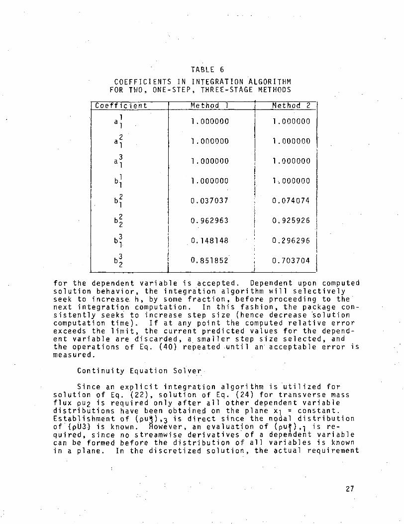
TABLE 6
COEFFICIENTS IN INTEGRATION ALGORITHMFOR TWO, ONE-STEP, THREE-STAGE METHODS
Coefficient
a]
'?'•
al
bi
b?
b2
bl
b2
Method 1
1 .000000
1 .000000
1 .000000
1.000000
0.037037
0.962963
0.148148
0.851852
Method 2
1 .000000
1 .000000
1 .000000
1,000000
0.074074
0.925926
0.296296
0.703704
for the dependent variable is accepted. Dependent upon computedsolution behavior, the integration algorithm w i l l selectivelyseek to increase, h, by some fraction, before proceeding to thenext integration computation. In this fashion, the package con-sistently seeks to increase step size (hence decrease 'solutioncomputation time). If at any point the computed relative errorexceeds the l i m i t , the current predicted values for the depend-ent variable are discarded, a smaller step size selected, andthe operations of Eq. (40) repeated until an acceptable error ismeasured. .
Continuity Equation Solver
Since an e x p l i c i t integration algorithm is u t i l i z e d forsolution of Eq. (22), solution of Eq. (24) for transverse massflux pu£ is required only after all other dependent variabledistributions have been obtained on the plane x-| = constant.Establishment of (pu$) ,3 is direct since the nodal distributionof {pU3} is known. However, an evaluation of (puf),] is re-quired, since no streamwise derivatives of a dependent variablecan be formed before the distribution of all variables is knownin a plane. In the discretized solution, the actual requirement
27

is to establish {pill}'; the following second-order accuratefinite difference formula for the derivative at the end pointof two panels of data of. dissimilar length is employed.
,* ' 1'n + h n + l >
In Eq. (42), h +; and h are the x-j integration step-sizes,respectively, Between tn<previous two stations.
le current X] station, xn + -| , and the
(42)
An analytic expression is then established for the X2distributions of mass flux derivatives, with X3 as a parameterand on a nodal basis, as
(pUl)' I ak(x,)x,k=0 K 6
(pU3),3 I MX3)Xk=0 K J(43)
thusing an n"" order running-smoothing polynomial generator overappropriate sequential panels of data. Using a unit step forthe weighting function, $, Eq . (24) then takes the form
(x
R
dx. (44)
m
Since all terms in Eq. (44) are integrals of perfect differen-ti a l s , the solution for the increment in transverse mass fluxover an interval Ax^ is directly obtained as
.. k+1A(pu*) I [a. (xj + b. (xj]
k = 0 k+1 (45)
Repeating Eq. (45) along each node column completes determinationof pui at the nodes of the transverse plane.
Computation of E q u i l i b r i u m Composition and ThermodynamicProperties of Hydrogen/Oxygen/Air Mixtures
The 3DBR Variant of COMOC can compute three-dimensionalfrozen flow m i x i n g of arbitrary gas mixtures, as well as the
28
e q u i l i b r i u m combustion of hydrogen/oxygen/air systems. For thelatter, the NASA computer code GAS (see Ref. 12) has been madeoperational within COMOC after considerable.modification to ren-der it compatible with a marching-type solution with m u l t i p l enodes, hence solutions. The e q u i l i b r i u m composition and thermo-dynamic properties of hydrogen/oxygen/air mixtures are evaluatedas a function of temperature and pressure; relative concentra-tions of the elements, H2, 02> N2, and Ar are also determined.The species considered are H20, u 2 , H2, N2, Ar, 0, H, NO, and OH.Since all th.ermophysical properties are temperature dependent,stagnation enthalpy is typically not known a priori; consequently,i n i t i a l i z a t i o n is based upon a user input total temperature dis-tribution. As a function of input pressure at i n i t i a l i z a t i o n andthe b u i l t - i n tables of thermodynamic data, distributions of statictemperature, frozen specific heat, and stagnation enthalpy cor-responding to input total temperature are determined using an it-eration algorithm based upon the method of false position. Allsolutions following initialization are based upon iteration toe q u i l i b r i u m composition using computed nodal static temperatureas the convergence parameter. The iteration on temperature isassumed to have converged when the difference between successiveiterates is less than 0.1 percent.
After convergence to a static temperature, the e q u i l i b r i u mconstants for chemical reaction are calculated from the G i b b s 1
function. Composition is then determined using a modified Newton-Raphson iterative procedure for solution of a system of nonlinearalgebraic equations. Once the nodal species equilibrium (or fro-zen) composition is determined, enthalpy, entropy, molecularweight, and specific heat are calculated for mixtures of idealgases in terms of the computed species mole fractions, Xa, as
Molecular Height: W
Specific Heat: c • "IW
a,,aI XaWa
a(«c.
(46)
(47)
Static Enthalpy: h
Entropy:
1 y xahaW L X n
a
li*"a
a| Inp - In Xa
(48)
(49)
Mass Fraction:
Gas Constant:
/ex
Y
.XaWa/W
- R/W
(50)
(51)
29
The e q u i l i b r i u m model is based upon the conservationproperties of the sum of mole fractions, and the constancy ofthe atomic number density ratios of argon/nitrogen, nitrogen/oxygen, and hydrogen/oxygen. The five chemical reactions con-sidered are
2H + 0 £"H20
2H * H2
20 J 02
H + 0 £ OH
+ 20 «- 2NO (52)
Applying the Law of Mass Action [Ref. 7] to each reaction inEq. (52), the following system of nonlinear algebraic equationsrelating species mole fractions, X^a', is obtained.
v(4) = v n.
(3)
(6)
(2)
(7) (53)
.thIn Eq. (53), K. is the e q u i l i b r i u m constant for the iu" reaction,which is ,a function of temperature only, and p is the staticpressure. The numbering scheme for species identification is1i sted i n Table 7.
TABLE 7
SPECIES IDENTIFICATION FOR REACTING HYDROGEN/OXYGEN/AIR SYSTEMS
Number
Chemical Species1 2 3
H OH H2
4 5 6
H20 0 02
7 8 9
NO N2 Ar
30

Equations for the conservation of total mass, and the i n d i v i d u a latomic species H, 0, N, and Ar, may be expressed in terms ofknown constants by the matrix equation.
{const.}
where
and
{const.} =
.00)(2)(3)(4)
The specific values of the constants cthe i n i t i a l composition.
(6)
(54)
[N3] sL a*
"l
1
0
0
_0
1110
0
12
0
0
0
12
1
0
0
1
0
1
0
0
10
2
0
0
1
0
1
1
0
10
0
2
0
l"
0
0
0
1_ (55)
(56)
are determined from
Of the several possible choices, the computed compositionis based upon solution of the nonlinear e q u i l i b r i u m equationsfor mole fraction of hydrogen, atomic oxygen, and the square rootof molecular nitrogen. The resultant n o n l i n e a r equation systemrequiring solution is
[fi(Xot)]{Xa} = {0} (57)
The N e w t o n - R a p h s o n i te ra t ion a lgo r i t hm a s s u m e s , g i v e n a set o ftrial v a l u e s , X", determinat ion of a new set of va lues Xn + 1 ,sepa ra ted from the Initial es t ima te by AXf t , by d i f ferent iat ingEq. ( 5 7 ) to y ie ld .
( 58 )
In Eq. (58), the Jacobian contains elements,. J k « , determinednumerically as
9f,
3Xa(59)
31

The n+1 es t imate of Xa is accep ted as the so lu t ion to Eq. ( 5 8 )when
3
I IMClH 1 e ( 6 0 ) 'j=l J " '
_5where e is a prescribed small parameter, usually 10 . A maximumof thirty iterations are allowed for the solution of Eq. (57)-(60) to converge w i t h i n e. In only a few cases has non-conver-gence occurred, always within a few degrees of the threshold tem-perature for dissociation. For these i n i t i a l l y divergent solu-tions, the equations are resolved assuming that dissociation isn e g l i g i b l e , i.e., the mole fractions of H, 0, OH, and NO are neg-l i g i b l y small in comparison to FU, G^* ^o' anc' ^?®'
ILLUSTRATIVE SOLUTIONS
.The 3DBR Variant of COMOC has established solutions forseveral two- and three-dimensional boundary region flows coveringa wide range of Mach and Reynolds numbers. Several are discussedto illustrate the various features of solution. The data decksfor two of these cases are presented in. the next section, andcome as standard test cases with the program.
Constant Density Flow Fields
Because of its basic simplicity, the two-dimensional, iso-energetic, laminar boundary layer flow of a fluid at small Machnumber (M < 0.3) provides an excellent check case for e v a l u a t i n gthe essential performance features of the finite element algo-rithm for Eq. (15)-(17). Only one dependent variable (u-|) needbe integrated numerically, along with solution of the continuity.equation for Up. However, COMOC assumes all flows are three-dimensional and compressible with temperature-dependent thermo-physical properties. The two-dimensionality is readily obtainedby specifying only one column of elements, see Fig. 4, and en-forcing the v a n i s h i n g normal gradient (q,n = 0) boundary condi-tion on the lateral segments of 3R. This is particularly simplesince v a n i s h i n g gradient is the automatic default value intrinsicto the finite element algorithm. The discretization may be ex-tended beyond the boundary layer thickness, 6X, so that v a n i s h i n gnormal gradient may be applied along the freestream segment of3R as well. The slope of the diagonals of the discretization,Fig. 4, bears l i t t l e impact on solution accuracy for two-dimen-sional problems. Dependent upon i n i t i a l conditions and/or otherperturbations placed into the solution, the computed variabledistributions along each node column may differ slightly. These
32
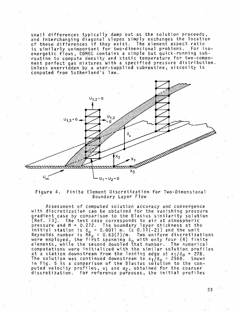
small differences typically damp out as the solution proceeds,and interchanging diagonal slopes simply exchanges the locationof these differences if they exist. The element aspect ratiois similarly unimportant for two-dimensional problems. For iso-energetic flows, COMOC contains a simple but q u i c k - r u n n i n g sub-routine to compute density and static temperature for two-compo-nent perfect gas mixtures with a specified pressure distributionUnless overridden by a user-supplied subroutine, viscosity iscomputed from Sutherland's law.
u
u
Figure 4. Finite Element Discretization for Two-DimensionalBoundary Layer Flow
Assessment of computed solution accuracy and convergencewith discretization can be obtained for the v a n i s h i n g pressuregradient case by comparison to the B l a s i u s simi1arity solution[Ref. .13]. The test case corresponds to air at atmosphericpressure and M = 0.272. The boundary layer thickness at the
= 0.0011 m. (E 0.11(-2)) and the unit. = 0.63(7)/m. Two uniform discretizations
6oRe,first spanning 60 with only four (4) finite
i n i t i a l station isReynolds number iswere employed, theelements, while the second doubled that number. The numericalcomputations were i n i t i a l i z e d with the similar solution profiles
downstream from the leading edge at x-|/60 = 278.was continued downstream to.x-|/60 = 2560. Showna comparison of the B l a s i u s solution to the com-
puted velocity profiles, U] and U2» obtained for the coarserdiscretization. For reference purposes, the i n i t i a l profiles
at a stationThe solutionin Fig. 5 is
33

are also shown with the finite element node locations superim-posed. The l o n g i t u d i n a l flow i n i t i a l l y contained w i t h i n 6 Q hasbeen retarded by a factor of 2 to 3 throughout, and agreementbetween the computed and Bl a s i u s velocity profiles is excellent.The computed skin friction and displacement thickness distribu-tions are shown in Fig. 6. The computations using the coarserdiscretization s l i g h t l y underpredict skin friction and overestimate displacement thickness. Doubling the discretization(to 8 elements lying within 6O) noticeably improves computedsolution agreement with the Bl a s i u s solutions, Fig. 6. Figure 7presents actual percent inaccuracy in the computed solutions forskin friction and displacement thickness. The influence of thecoarse discretization is most noticeable in 6; however, the errorrapidly decreases as the boundary layer grows into the discreti-zation, which corresponds essentially to grid refinement. As afunction of discretization, computed skin friction, Cf, convergesapproximately proportional to the square of refinement. Thisagrees exactly with the convergence rate predicted theoreticallyfor the parent diffusion equation, neglecting convection, usinglinear finite element approximation functionals [Ref. 14]. Theuniformily small inaccuracies in computed skin friction for bothdiscretizations indicate that solutions, adequate for certainengineering approximations, can be obtained using finite elementdiscretizations that app.ear rather coarse in comparison to con-ventional experience.
1.0 2.0
Transverse Coordinate-
Figure 5. Computed Velocity Distributions, M = 0.272,ReY = 0.63(7)/m
/\
34

0.25
0.20
x 0.15o"
0.10
0.05Symbol
—
A
O
Solution
BlasiusCOMOC
COMOC
No. Elements •Spanning 6O
48
3.5
3.0
2.5
2.0
I
1.5
1.0
1000 2000Longitudinal Coordinate - Xi/8o
3000
Figure 6. Computed Skin Friction and Boundary Layer Thickness,M = 0 . 2 7 2 , Rev = 0 . 6 3 ( 7 ) / m
/\
10
1X1cO
1 4O
10
Symbol
A
0
No. ElementsSpanning 5,,
4
8
A\\ 5\
1000 2000Longitudinal Coordinate - *i/
3000
Figure 7. Computed Solution Accuracy and Convergence,M = 0.272, Rev = 0.63(7)/m
A *
35
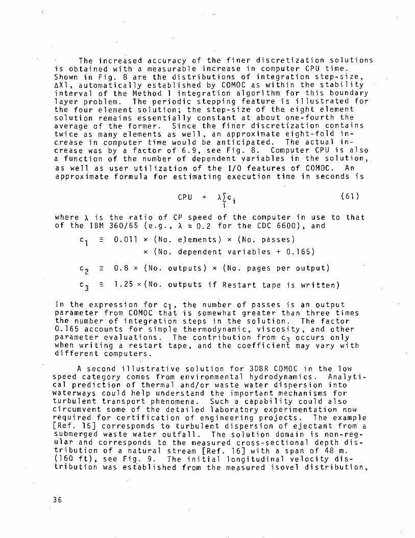
The increased accuracy of the finer discretization solutionsis obtained with a measurable increase in computer CPU time.Shown in Fig. 8 are the distributions of integration step-size,AX1 , automatically established by COMOC as within the stabilityinterval of the Method 1 integration al gori thm f or this boundarylayer problem. The periodic stepping feature is illustrated forthe four element solution; the step-size of the eight elementsolution remains essentially constant at about one-fourth theaverage of the former. Since the finer discretization containstwice as many elements as w e l l , an approximate eight-fold in-crease in computer time would be anticipated. The actual in-crease was by a factor of 6.9, see Fig. 8. Computer CPU is alsoa function of the number of dependent variables in the solution,as well as user u t i l i z a t i o n of the I/O features of COMOC. Anapproximate formula for estimating execution time in seconds is
CPU = \lc. (61)
where X is the ratio of CP speed of the computer in use to thatof the IBM 360/65 (e.g., X ~ 0.2 for the CDC 6600), and
c, E 0.011 x (No. elements) x (No. passes)
x (No. dependent variables + 0.165)
Cp = 0.8 x (No. outputs) x (No- pages per output)
c3 = 1.25x(No. outputs if Restart tape is written)
In the expression for c-j , the number of passes is an outputparameter from COMOC that is somewhat greater than three timesthe number of integration steps in the solution. The fa-ctor0.165 accounts for s i m p l e thermodynami c , viscosity, and otherparameter evaluations. The contribution from Co occurs onlywhen writing a restart tape, and the coefficient may vary withdifferent computers.
A second i l l u s t r a t i v e solution for 3DBR COMOC in the lowspeed category comes from environmental hydrodynamics. Analyti-cal prediction of thermal and/or waste water dispersion intowaterways could help understand the important mechanisms forturbulent transport phenomena. Such a c a p a b i l i t y could alsocircumvent some of the detailed laboratory experimentation nowrequired for certification of engineering projects. The example[Ref. 15] corresponds to turbulent dispersion of ejectant from asubmerged waste water outfall. The solution domain is non-reg-ular and corresponds to the measured cross-sectional depth dis-tribution of a natural stream [Ref. 16] with a span of 48 m.(160 ft), see Fig. 9. The i n i t i a l l o n g i t u d i n a l velocity dis-tribution was established from the measured isovel d i s t r i b u t i o n ,
36

80
-=. 60x
40CO
Q.<U1-1COco
« 20c
Symbol
A
O
No. ElementsSpanning 6n
4
8
CPU360/65141
973
0 1000 2000 3000Longitudinal Coordinate - x t/5o
Figure 8. Integration Step-Size Distribution,
M = 0.272, ReY = 0.63(7)/m/\
Velocity m/s
Figure 9. Cross-Section of a Natural Stream
Showing Measured Isovels, [Ref. 16]by interpolation at the nodes of a 468 finite element discreti-zation of the cross-section, see Fig. 10. .Since the solutiondomain is quite non-regular, the automatic discretizer in COMOCwas not a p p l i c a b l e . The waste water ejector was assumed locatedin the deepest section of the river as shown in Fig. 10.
A Initial 100% Contour
Figure 10. Finite Element Discretization of Stream Cross-Section
37

The flow field was assumed isoenergetic and without cross-flow. Hence, a marching type solution was required for m a i n -stream velocity and a s i n g l e species mass fraction. The totaland static temperatures for this case are i d e n t i c a l ; thus, alarge input pressure was employed to coerce the perfect gas sub-routine in COMOC to compute a uniform density distribution cor-responding to that of water. Closure of the governing equationsystem was obtained by specifying a turbulent viscosity law, andproviding a user-written subroutine to override Sutherland's LawA tensor turbulence law was assumed a p p l i c a b l e [Ref. 17, 18];in the plane of the finite element discretization, the eddy vis-cosity coefficients in the vertical (/2) and transverse (x3)coordinate directions were assumed given as
y*2 = k2U*h . (62)
y*3 = k3U*h (63)
where local depth of water is g i v e n by h, k2, and k3 are empir-ical constants, and U* is the friction velocity defined asU* = /T/P. The approach of Patankar and Spalding [Ref. 19] wasemployed to evaluate w a l l shear, T, as.
T = K2pU2[R"] - 0.156R"0'45 + 0.08723R'0'3X X X
+ 0.03713R"0'18] (64)A ,
2where K is an empirical constant (set equal to 0.435,), Rx =, RKwhere R is a local Reynolds Number defined as R = pffx^/y, U islocal l o n g i t u d i n a l velocity near its extremum, and X2 j,s a rep-resentative length scale. For the present case, both U and X2were obtained directly from the solution for the detailed veloc-ity profiles. A study was performed, see Table 8, to measurethe sensitivity of the computed p o l l u t a n t distribution to theconstants in the eddy viscosity law, Eq. (62)-(63), as well asthe te.nsor character. The base l i n e case corresponds to useof mean depth averages for the coefficients, confirmed experi-mentally .to capture the essential parabol ic character of themeasured distributions, Case II. Case III corresponds to ascalar eddy viscosity equal to the magnitude of the Case Itensor expression.
The results obtained from this type of study are summarizedin Fig. 11, which presents predicted mass fraction contours ofthe contaminant, for the three cases, at a station 9.6 m. down-stream of injection. Comparing the results of Cases I and II,the neglect of the p a r a b o l i c distribution in the vertical m i x i n g
38

T A B L E 8 '
P A R A M E T E R S IN P O L L U T A N T D I S P E R S I O N STUDY
Case
I
II
III
k2
0.067
0.36U-S2)
0.24
k3
0.23
0.23
0.24
Comments
Base line case [Ref. 16]
Vertical p arabolic distribution(£=nondimensional local depth)
Scalar of equal magnitude toCase I
15%
0.1%30%
, Case 111
Figure 11. Predicted Mass Fraction Contours at 9.6 m Downstreamof Injection, Three Diffusion Models
coefficients is confirmed to be a reasonable assumption at thisdistance downstream. However, for these conditions, the omissionof the tensorial character of the dispersion, coefficient, CaseI I I , is quite measurable. Comparing Cases III and II, the largervertical (k£) coefficient has allowed the 3% contour to break tothe surface of the river. An overall larger diffusion has also
39

occurred, although, as expected, the lateral extent of the dis-tributions is considerably less affected. Although no experi-mental data are a v a i 1 a b l e to directly confirm these results, thesepredictions amply illustrate the potential to examine trends andisolate key features, w h i l e capturing the important geometricnon-regularities and differential equation non-linearities soimportant to the physics of the problem. The numerical procedureis readily adaptable to relocation of the ejector and alterationof its geometry, see Fig. 12 for example. For all cases, inte-gration was continued downstream a distance of approximately 90 m;at this point the maximum ejectant concentration had decreased to
Y///////A Initial 100% Contour
0.1% 0.1%
Figure 12. Predicted Mass Fraction Contours at 9.6 m Downstreamof Interface Injection
15% ±1% dependent upon the viscosity law. A typical executiontime on the IBM 360/65 was 875 s i n c l u d i n g about 145 s to producean inch of output. The predicted v a l u e using Eq. (61) is 900 s.(It should be noted that, a l t h o u g h tensor turbulent transportproperties can be u t i l i z e d in 3DBR, program modification, beyondthe scope of the casual user, is required for the present Variant
Compressible Flow Fields
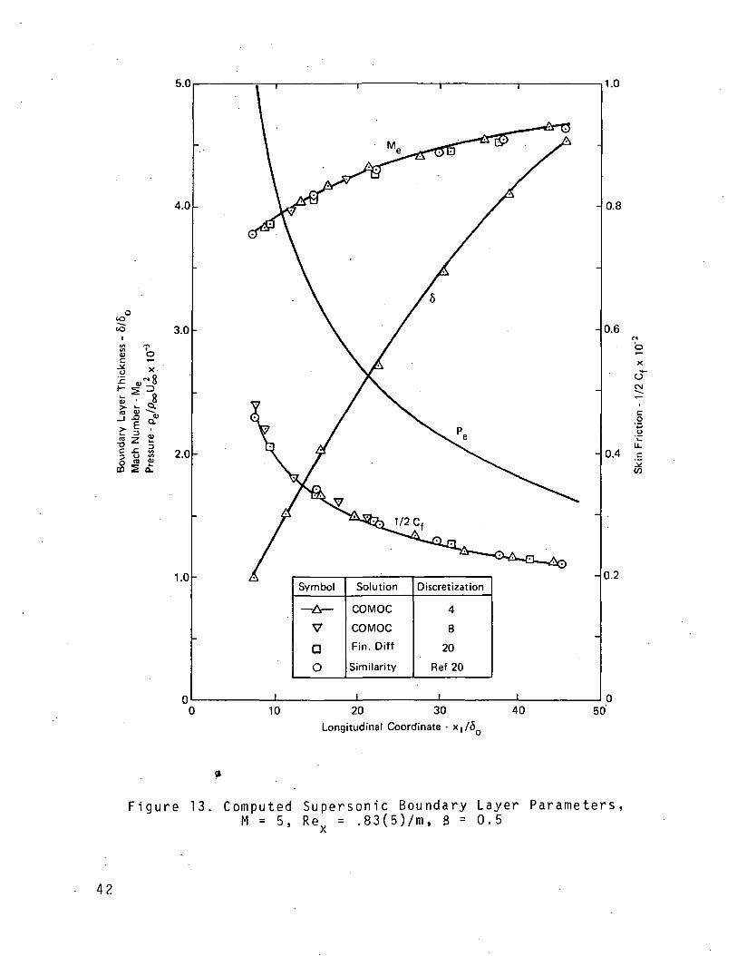
A standard checkMach 5. laminar, two-dibatic wall in a favoration [Ref. 20], as we!utilized to evaluate afor the detailed couplthis solution. The dications are essential!ber boundary layer solcorresponds to the simsubroutine can be useddensity for isoenergetintegrated downstream,
case for 3DBR COMOC corresponds to a nominalmensional boundary layer flow over an adia-ble pressure gradient. A similarity solu-1 as finite difference procedures, can beccuracy and consistency of solution trendsing of the mechanics and thermodynamics ofscretization and boundary condition specifi-y i d e n t i c a l to those of the small Mach num-ution. For constant specific heat, w h i c h "ilarity solution, the s i m p l e thermodynamicto compute local static temperature and
ic flow. Only the equation for ui need becoupled with solution for U2 using the
40
continuity equation solver. For non-isoenergetic flow or variablespecific heat, stagnation enthalpy (H) must be added to the inte-grated solution vector, and the local solutions for density,static temperature, and specific heat are obtained from the com-bustion subroutine. In this instance, the air composition mustbe i n i t i a l i z e d as well, although the oxygen and.nitrogen 'elementalspecies mass fractions need not be integrated since the flow f i e l dcomposition is homogeneous and constant. For either thermodynamicprocedure, the stagnation enthalpy is i n i t i a l i z e d from an input(constant) total temperature distribution. The i n i t i a l U] pro-files are established from the s i m i l a r solution for 3 = 0.5 andS = 0 [Ref. 20]. Sutherland's law is employed to computeviscosity.
The standard test case is i n i t i a l i z e d at xi = 0.03 m down-stream from the surface leading edge. The boundary layer thick-ness at this station is 6g = 0.0039 m, the local Mach number isM =? 3.77, the unit Reynolds number is Rex = ,83(5)/m, and theadiabatic wall temperature is Tw = 1000°K (1800°R). Shown inFig. 13 are the COMOC computed skin friction, freestream Machnumber, and .boundary layer thickness distributions for the con-stant specific heat case. These were obtained using two uniformfinite element discretizations corresponding to 4 and 8 elementsspanning the initial boundary layer thickness. The input staticpressure d i s t r i b u t i o n , Pe(*l)> is also presented for reference,and the boundary layer thickness has increased, greather thanfour-fold within the solution domain. Only small differences,on the order of about 2%, exist between the two solutions, withthe finer discretization producing a s l i g h t l y larger skin fric-tion and smaller freestream Mach number. Superimposed in F i g .13, for.comparison purposes, are the results for the s i m i l a rsolution [Ref. 20], and a 20 zone finite difference solution ob-tained using the von Mises coordinate transformation [Ref. 19].Agreement among the four solutions is excellent (within 2%) forskin friction. The s i m i l a r solution for M e l i e s between theCOMOC and finite difference solutions, and agreement is within±3%. Shown in Fig. 14 are computed velocity profiles at X]/60 =22.7, which is about mid-way through the standard test solutiondomain. Shown for reference is the i n i t i a l U] profile obtainedfrom the s i m i l a r solution [Ref. 20], with the node locations ofthe 4 element discretization superimposed. Both COMOC solutionsproduce U] distributions that are s l i g h t l y more concave upwardin the mid-region in comparison to the s i m i l a r i t y or finitedifference solutions. The finer discretization COMOC solutionl i e s closer to the s i m i l a r i t y solution in the region where thetwo finite element solutions differ. The finite differencesolution l ies appreciably below both the COMOC and s i m i l a r i t ysolutions near freestream. The COMOC computed transverse veloc-ities are also shown in Fig. 1.4; .only s l i g h t differences betweenthe two discretization solutions, are apparent. The trends of
41
5.0
4.0
<otoi
s/> f>in »<B O
"
3.0
£> E r|z Sc .c 3
111
2.0
1.0Symbol
-&-
V
D
0
Solution
COMOC
COMOC
Fin. Diff
Similarity
Discretization
4
8
20
Ref 20
1.0
0.8
0.6
0.4
o
X*4-
OCM
O
c
w
0.2
10 20 30
Longitudinal Coordinate •
40 50
Figure 13. Computed Supersonic Boundary Layer Parameters,M = 5, Re = .83(5)/m, 8 = 0 . 5
42

.*. 0.10
1.00
0.50
0.25
*'/5o
7.6
22.7
22.7
22.7
22.7
X
V
-A-
O
B
Solution
Initial
COMOC (4 Elements)
COMOC (8 Elements)
Similar [Ref 20]
Finite Difference
0.5 1.0 1.5 2.0
Transverse Coordinate - x2/8
Figure 14. Computed Supersonic Boundary Layer VelocityM = 5, Rev = .83(5)/m, 3 = 0.5
X
43

the COMOC solutions are in excellent agreement with the estab-lished procedures; unfortunately, since each method of solutionis distinctly numerical, no absolute accuracy assessment isestablished, as was possible for the constant density boundarylayer check case.
The computation of transverse velocity warrants a d d i t i o n a lcomment. COMOC w i l l accept, but does not require (since one israrely a v a i l a b l e ) , an i n p u t distribution for U2 at the i n i t i a lstation. For the discussed Mach 5 solutions, the i n i t i a l U2distribution, Fig. 14, is self-determined by w i t h h o l d i n g itscomputation un t i l the u^ equation had been integrated forwarda few stations. (This is mandatory, even if an i n i t i a l U2distribution is input, since several data stations are requiredto a l l o w evaluation of Eq. (42) for (pu-|)'.) Computation of U2is then initiated and it rapidly becomes consistent with thecomputed u] distributions. Solution is terminated after a fewmore steps downstream, and the computed nodal 02 distributiontrend with l o n g i t u d i n a l distance is back extrapolated to estimatean i n i t i a l distribution. Only one or two iterations of this typeare typicaVly required to establish a consistent U2 distribution.Starting with a zero i n i t i a l d i s t r i b u t i o n is probably the mostconvenient choice for analysis of engineering problems, whereindetailed i n i t i a l accuracy is not of primary importance.
Solution speed and accuracy have been i1lustrated • to deoenddirectly upon discretization. Solution speed is also a directfunction of a user i n p u t control parameter (e) that places some-what flexible bounds on acceptable relative truncation error,Eq. (41), during downstream integration. A va.lue of e of 10(-4)has been found by experimentation to be generally adequate tom a i n t a i n solution stability, hence accuracy. Using smaller valuesof e sharply increases computation time without producing theattendant increase in solution accuracy that a finer discretiza-tion would yield. However, increasing e up to 10(-2) can producemeasurable cost savings with a good probability of only a marginaldecrease in solution stability and accuracy (upon rare occasion,the solution may actually go unstable and blow-up). Shown inFig. 15 are computed integration step-size histories for theMach 5 .test case for several discretizations and values of e.In all cases, the computed solutions were of comparable accuracyand uniformly acceptable. The automatic stepping feature isillustrated, and the predicted necessary sharp decreases in Ax-|appears independent of e. For the two, 8-element discretizationtests, increasing c to 10(-2) about doubled the allowed step sizeand hence decreased CPU by almost 50%. As expected, a four-foldincrease in CPU accrued for twice the discretization, for e con-stant at 10(-4), with integration step-size about half that ofthe baseline 8-element case. The coarsest 4-element discretiza-tion test recorded the largest integration step distribution witha remarkably smaller CPU. However, this solution appeared on the
44
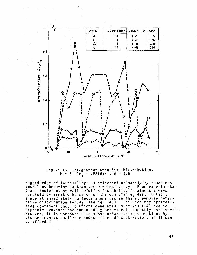
I
(D
ao>
c• o
£ 0.4 -
Longitudinal Coordinate
Figure 15. Integration Step Size Distribution,M = 5, Rev = .83(5)/m, 6 = 0.5
/\
ragged edge of i n s t a b i l i t y , as evidenced primarily by sometimesanomalous behavior in transverse velocity, U£. From experimenta-tion, i n c i p i e n t overall solution instability is almost alwaysforetold by erratic behavior of the computed u2 d i s t r i b u t i o n ,since it immediately reflects anomalies in the streamwise deriv-ative distribution for UT, see Eq. (45). The user may typicallyfeel confident that solutions generated using e>10(-4) are ac-ceptable provided the computed U2 behavior is smoothly consistentHowever, it is worthwhile to substantiate this assumption, by ashorter run at smaller e and/or finer discretization, if it canbe afforded
45
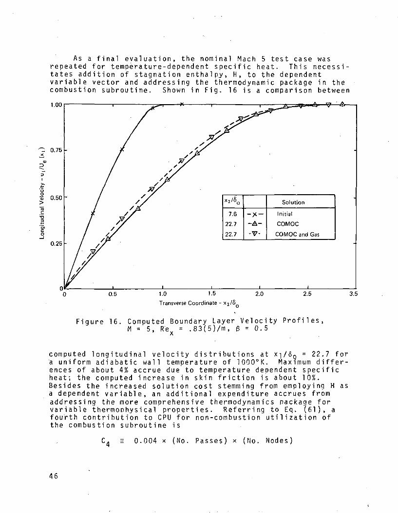
As a final evaluation, the nominal Mach 5 test case wasrepeated for temperature-dependent specific heat. This necessi-tates addition of stagnation enthalpy, H, to the dependentvariable vector and addressing the thermodynamic package in thecombustion subroutine. Shown in Fig. 16 is a comparison between
1.00
1.0 1.5
Transverse Coordinate - x2/5
Figure 16. Computed Boundary Layer Velocity Profiles,M = 5, Rev = .83(5)/m, 6 = 0.5
X
computed l o n g i t u d i n a l velocity d i s t r i b u t i o n s at X]/6Q = 22.7 fora uniform adiabatic wall temperature of 1000°K. Maximum differ-ences of about 4% accrue due to temperature dependent specificheat; the computed increase in skin friction is about 10%.Besides the increased solution cost stemming from employing H asa dependent v a r i a b l e , an additional expenditure accrues fromaddressing the more comprehensive thermodynamics package forvariable thermophysical properties. Referring to Eq. (61), afourth contribution to CPU for non-combustion utilization ofthe combustion subroutine is
C, = 0.004 x (No. Passes) x (No. Nodes)
46

The second example problem for compressible flow computa-tions using 3DBR COMOC corresponds to analysis of turbulent,binary three-dimensional m i x i n g in a supersonic boundary layerflow fiel.d. The analyses include cold flow studies with com-parison to data as well as e q u i l i b r i u m combustion. The impetusfor these studies is the hydrogen fueled scramjet engine, aprominent candidate for propulsion of the next generation ofhypersonic cruise vehicles [Ref. 21, 22]. Many alternativedesigns have been proposed, but all e x h i b i t the commonality thatfuel introduction arrangements consist of rows of circular,choked-flow injector orifices mounted flush or normal to thecombustor wall or in fins spanning the combustor inlet. Thepattern of fuel injection, hence three-dimensional mix.ing, canexert significant influence on combustor performance. Figure 17illustrates an experimental apparatus used by Rogers to experi-mentally probe the three-dimensional cold m i x i n g region down-stream of transverse hydrogen injection from .a single discreteorifice [Ref. 23], an;d mul ti pi e laterally-disposed orifices[Ref. 24], into a Mach 4 airstream on a flat plate. Detailednumerical predictions of turbulent, three-dimensional m i x i n g in
60
Flat Plate
Injection Orifice
Figure 17. Three-Dimensional Flow Fi e l d Downstream ofTransverse Injection from Discrete Orifices
47

this flow field have been performed, using 3DBR COMOC, in a so-lution domain spanning up to 120 injector diameters downstream,for both the s i n g l e and m u l t i p l e jet geometries. The scaleddiscretization of the symmetric half-plane into 100 finite ele-ments, Fig. 18, was formed by the automatic discretizer. Theturbulent boundary layer thickness at the injector station(without injection) was equal to 2.7 injector diameters, andthe Reynolds number was Rex = .6(8)/m. To the firstapproximation, these data correspond to isoenergeticdiffusion in a constant pressure flow field. Hence,integration was required for u-| and a single speciestion p.lus the continuity equation for u9.
order ofbi narynumeri calmass frac-
Closure of the equation .system requires a turbulence modelfor three-dimensional boundary region flow of this type. Aprototype eddy viscosity model was developed to reflect massflux differences between the main flow and the jet and the tur-bulence due to the presence of the wall [Ref. 25]. Directlyabove the m i x i n g region, turbulent dispersion was assumed toprimarily reflect differences in mass flux. Outside the m i x i n gregion but near the w a l l , the turbulence was assumed due solelyto boundary layer phenomena. W i t h i n the m i x i n g region bothmechanisms are assumed active. Therefore, near the wall where
co>
<uu
JtO
cCO
10.0r
8.0
6.00
4.00
2.00
0.00 L
0.00 2.00 8.00 10.00
Figure 18.
4.00 6.00Lateral Displacement - x3/D
Fi rn te.Element Discretion of Symmetric Half-Spaceof Single-Jet Injection Geometry
48

m i x i n g length theory ismass is of the form
assumed v a l i d , the eddy diffusivity of
3U-
3x, Sc -1 (65)
u 1 is the mean l o n g i t u d i n a l velocity, £ is the m i x i n g length,w'is va.n Driest's damping factor [Ref. 26], and y is the inter-mittency factor, empirically modeled in a number of ways [Ref.27]. For this study, it was evaluated as
1
1 + O.OU'(66)
where r, = X2/6;?» and ^2 is tne value of X£ where the hydrogenmass fraction is one-half its wall value. In the outer regionthe eddy diffusivity of mass is assumed proportional to themass defect of the form
(67)
where K is an empirical constant, y is the intermittency factor,the characteristic length L is defined as the half height of them i x i n g region on the centerplane (xj = 0), and I is the three- .dimensional mass defect evaluated as
KX-,) (68)
A subroutine was coded for addition to 3DBR-COMOC, to evaluateEq. (65)-(68) along columns of nodes parallei to the x.2 axis,see Fig. 18. The effective viscosity of mass mixing was laminarplus selectively E] or e2» and the transition from e-j to £2 wasinternally signaled. So as to provide the potential user withan example of construction of a fairly complex subroutineaddition, this code forms a part of the data deck for the secondstandard test case for 3DBR-COMOC.
An extensive computational program was conducted using3DBR-COMOC to validate use of the three-dimensional boundaryregion equations for this problem geometry, and to evaluatethe governing influences on turbulent m i x i n g in the three-dimensional region within the constraints of the prototype eddyviscosity model. The existence of extensive cold flow data[Ref. 23, 24] for l o n g i t u d i n a l vel oci ty , u-i , and hydrogen massfraction, YH, provides the means to evaluate the accuracy and
49
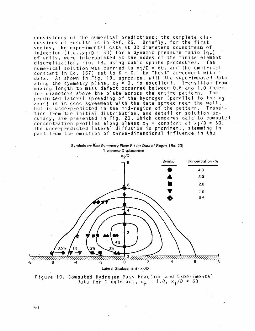
consistency of the numerical predictions; the complete dis-cussions of results is in Ref. 25. Briefly, for the firstseries, the experimental data at 30 diameters downstream ofinjection (i.e.,xi/D = 30) forof unity, were interpolated atdiscretization, Fig. 18, usingnumerical solution was carriedconstant in Eq. (67) set to K
a dynamic pressure ratio (qr)the nodes of the finite elementcubic s p l i n e procedures. Theto x-|/D = 60, and the empirical
= 0.1 by "best" agreement with 'data. As shown in Fig. 19, agreement with 'the superimposed dataalong the symmetry pl a n e , X3 = 0, is excellent. Transition fromm i x i n g length to mass defect occurred between 0.6 and 1.0 inje'c-tor diameters above the plate across the entire pattern. Thepredicted lateral spreading of the hydrogen (parallel to the X3axis) is in good agreement with the data spread near the wall,but is underpredicted in the mid-region of the pattern. Transi-tion from the i n i t i a l distribution, and detail.on solution ac-curacy, are presented in Fig. 20, which compares data to computedconcentration profiles along planes x^ = constant at x^/D = 60.The underpredicted lateral diffusion is prominent, stemming inpart from the omission of three-dimensional influence in the
Symbols are Best Symmetry Plane Fit for Data of Rogers [Ref 23]Transverse Displacement
Concentration - %
-6 - 2 0 2
Lateral Displacement - x-j/D
Figure 19. Computed Hydrogen Mass Fraction and ExperimentalData for Single-Jet, qr = 1.0, x^D = 60
50

Symbol Description
AA
Initial Conditions, x^D = 30Raw Data MeasurementsBest Symmetry Plane DeterminationCOMOC Computation
8 0 2 4 6 0 2 0 0
Hydrogen Mass Fraction • Y (%)
Figure 20. Computed Single-Jet Hydrogen Mass FractionDistribution at x^D = 60, qr = 1 . 0
turbulence model. The experimental data show that in this re-gion, ui,2 and Ml,3 are of equal magnitude, as observed in Fig.21, which is a three-dimensional surface plot of the longitudinalvelocity distribution at x-|/D = 30, as observed from a vantagepoint beneath the plate surface. The superimposed grid coincideswith the finite element discretization (omitting diagonals), andthe hydrogen jet is imbedded within the centroidal indentation.Obviously, three-dimensional effects are important, and shouldform an integral part of future three-dimensional turbulencemodeling. Figures 22 and 23 compare the COMOC computed solutionsfor hydrogen mass fraction and l o n g i t u d i n a l velocity distribu-tion to data at x-j/D = 120, as well as the i n i t i a l distributions.Agreement is generally quite good throughout.
This computational study was repeated using for i n i t i a lConditions the experimental data for a row of orifices alignedperpendicular to the main flow vector with a uniform separationdistance of 12.5 orifice diameters [Ref. 24]. For this study,the finite element discretization of Fig. 18 was simply scaledto span the symmetric half zone between ejectors, using theautomatic discretizer. The van i s h i n g normal gradient boundarycondition was then applied to both lateral sides of the compu-tational region. Shown in Fig. 24 and 25 are the COMOC com-puted hydrogen mass fraction profile distributions at stationsX]/D = 60 and x-|/D = 120 compared to data. .Figure 26 displaysthe more familiar contour plot at x-|/D = 120. These results
51

Centerplane
Fi gure 21. Isometric View of Longitudinal Velocity SurfaceSingle-Jet Configuration, x-|/D = 30
for
Symbol Description
Initial Condition, Xj /D = 30
Raw Data Measurements
x3/D = 0
Best Symmetry Plane DeterminationCOMOC Computation
x3/D
= 6.5
0 4 6 8 0 2 4 6 0
Hydrogen Mass Fraction Y (%)
Figure 22. Computed Single-Jet Hydrogen Mass FractionDistribution at x,/D = 120, q^ = 1.0
52

Symbol DescriptionInitial Condition, Spline Fit, X../D = 30
Experimental Data, x.j/0 = 120
COMOC Computation, Xj/D = 120
10
CMX
OJ ~E 6ID'CJCO
Q 4
§ 2I-
x3/D = 0 x3/D= 1.0 x3/D = 2.5 x3/D = 4.5
1000 2200 ' 1000 2200 1000 2200 1000Longitudinal Velocity - u. (ft/sec)
2200 1000 2200
_| L fc I 1 I 1 f ill I I I I I - t i I 1 I I I i i
nn "• onn cnr> Tnn * onn cnn inn ' onn cnn inn '•omi i i
300 500 700 ' 300 500 700 300 500 700 300 500 700 ' 300 500 700Longitudinal Velocity - u^ (m/sec)
Figure 23. Computed. Single-Jet Longitudinal VelocityDistribution at x^D = 120, qr = 1.0
—i_. Symbol1 Description • - - —
Initial Conditions, x^D = 30;
O Raw Data Measurements• Best Symmetry Plane Determination
COMOC Computation
x3/D
4.5
0 2 4 6 0 2
Hydrogen Mass Fraction - Y (%}
Figure 24. Computed Multijet Hydrogen Mass FractionDistribution at x^/D = 60, q - 1.0
53

Symbol Description
Initial Conditions, x.j/0 = 30
© Raw Data Measurements9 Best Symmetry Plane Determination
COMOC Computation
x3/D = 0 x3/D = 1x3/D = 6.25
OK)
6 0 2 4 6 0 2
Hydrogen Mass Fraction - Y (%)
0 20 20
Symbols
T
Figure 25. Computed Multijet Hydrogen Mass FractionDistribution at x-j/D = 120, qp = 1.0
Concentration — %
V
O
2.2
2.0
1.5
1.0
0.5
0.25
Symbols are Best SymmetryPlane Data of Rogers [Ref 24]
Transverse Displacement - Xj/D
8
0.25%
V0.5%
- 2 0 2
Lateral Displacement - X
Figure 26. Computed Mass Fraction Contours and ExperimentalData for Multijet, X/D = 120, q = 1.0

were obtained using the identical m i x i n g model of the s i n g l ejet, i.e., K = 0.1, Eq. (67), with transition from m i x i n g lengthto mass defect occurring in the region 0.6 <_ x;?/D <_ 1.1. Figures24 and 25 indicate that centerplane diffusion is somewhat over-predicted, while a considerable improvement between computationsand data has occurred in the lateral region. Figure 26 i l l u s -trates how the computed contour patterns merge between jets forthe m u l t i p l e injector configuration. Agreement between computedand measured velocity distributions at both downstream stationswas excel lent.
Detailed volumes of experimental data, of the tyoe uti1ized.to start these discussed solutions, are typically not a v a i l a b l efor complex reacting flow fields. Assuming that the foregoingstudies have indeed verified the appropriateness of the differ-ential equation system, as well as a limi t e d v a l i d i t y for theturbulence model, methods for starting a three-dimensional solu-tion with combustion are sought. One technique that shows somepromise, and also admits numerical evaluation of its appropriate-ness, is the "virtual source." The theoretical hypothesis issimply that the complex transverse injection process can be com-putationally replaced by a hydrogen jet imbedded w i t h i n a boundaryregion flow, and that the d i s t i n g u i s h i n g features of this virtualsource are solely dependent upon freestream and injectant param-eters. The derived model [Ref. 25] captures the essence of thebarrel shock-Mach disk hypothesis for injectant-freestream equi-libration [Ref. 28]. To establish computational verification ofthis concept, the cold flow studies were repeated for the virtualsource established in the plane of injection, i.e., x,/D = 0.0.It was assumed to be of e l l i p t i c a l cross-sectional shape with theminor axis parallel to X2» and composed of 100% hydrogen withl o n g i t u d i n a l momentum determined from the dynamic pressure ratio,qr. Computational evaluations of the concept were made for thethree values of qr for which data exist. Shown in Fig. 27 aretypical results, obtained for virtual source simulation of them u l t i p l e injection configuration for qr = 1.0. Superimposed areappropriate experimental data [Ref. 23, 24] for the key comparisonbases of, 1) l o n g i t u d i n a l trajectory of maximum hydrogen concen-tration, 2) height above the plate of the maximum concentrationtrajectory, and 3) the lateral spreading of the diffusion pattern.The peak hydrogen mass fraction is observed to drop precipitouslyfrom its i n i t i a l 100% concentration, but to promptly level off ingood agreement with the multijet data. The deoendent variablegradients associated with this solution were quite large, yet3DBR-COMOC maintained stable solution behavior using the automaticstep-size constraint. The trajectory of the maximum hydrog.en con-centration above the plate surface is s i m i l a r l y in good agreementwith multi-jet data. The computed lateral spreading agrees wellwith multi-jet data to x-|/D = 30, but is progressively underpre-dicted (maximum 15%) as the solution continues downstream. Simi-lar agreement trends with data were recorded for the "softer"
55 .
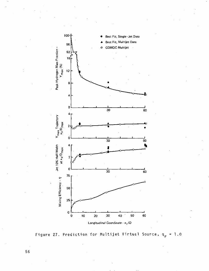
100
O)c
50
25
• Best Fit, Single-Jet Data
A Best Fit, Multijet Data
o COMOC Multijet
0 «»wO
— >
fri
0
7530 60
10 20 30 40
Longitudinal Coordinate -
50 60
Figure 27. Prediction for Multijet Virtual Source, q = 1.0
56

injection case,- qr = 0.5. However, fairly large disparities (upto 40%) occurred for the "hard" jet, corresponding to qr = 1.5,but for which the entire theoretical concept becomes rather sus-pect. Figure 27 is completed with a plot of n., an integral"mixing efficiency" parameter, [Ref. 24]. This parameter isdefined as the percentage of molecular hydrogen that would belost to the computed frozen flow H;? mass fraction d i s t r i b u t i o nif all a v a i l a b l e \\% (or 0;?, depending on the l i m i t i n g reagent)was converted to HpO within the computed velocity distribution.
The virtual source turbulent transport model was identicalto the prior cold flow studies with two minor exceptions. Them i x i n g length hypothesis, e-| , was uniformly enforced until theminimum velocity in the virtual source depression accelerated towithin ~2% of the corresponding boundary layer velocity withoutinjection. This occurred within 8 diameters downstream of theinjection Diane for all qr. Downstream of xi/D = 8, transitionfrom e] to £2 occurred w i t h i n one diameter above the Plate sur-face. Due to the rather small i n i t i a l density within the virtualsource, the i n i t i a l computed mass defect was disoroportionallysmall. From exnerimentation, a smaller constant (K = 0.05) wasfound uniformly effective for the three studies.
With the change of one input flag, the virtual sourcesimulation was repeated with e q u i l i b r i u m combustion allowed.Shown in Fig. 28 are the typical results of this computationalsimulation, on the m u l t i p l e comparison bases previously dis-cussed for the cold flow tests. The precipito.us drop in the.peak hydrogen mass fraction concentration parallels the coldflow experience, but the levels downstream of x-|/D = 7 lie wellbelow the non-reacting experience. The trajectory of the peakhydrogen level is essentially parallel to the plate surfacethrough x^/D = 30. The lateral spreading of the jet is con-siderably more pronounced for X]/D>10 in comparison to the coldflow tests. The mixing efficiency parameter, ri, reaches 100%at x-|/D = 20, well ahead of the cold flow simulation. Thesedifferences reflect, in large part, the considerably differenttemperature and density distributions. As shown in Fig. 28,i g n i t i o n occurs immediately downstream of simulated injection,and the peak temperature rapidly climbs to 2000°K (~3800°R).It remains at this level until stoichiometric m i x i n g is corn-Dieted, i.e., n = 100%; thereafter, it continuously decreasesas local heat addition from combustion is unable to balancediffusion effects. A typical CPU time on the IBM 360/65 forexecution of this test with combustion was about 1275 seconds.Execution of a cold flow counterpart (to x-j/D = 30) requiredabout 950 seconds. The 325 seconds a d d i t i o n a l for combustionreflects the CPU required to execute the temperature iterationloop in the combustion subroutine for this particular test case.
57

oCO
-
S <3<
//1
1
3 0 0 C
B oo
CM •—
OCO
Oin
0
'*
oCO
oCM
O
O>
Q
X*1
4WCO
_c13
O
3CQC
3
O
ns_
cr
on3CU
CTLU
ooo
t
oCO
oin
CDC
o T?CO o
oo~co
a Icn
O
OO
in o inft. in CM
i-o
EO
CDt-Q.
00CN)
O)
O)
6ujx;|/\|
58

DATA DECK PREPARATION
The data decks that generate the nominal Mach 5 isoenergeticboundary layer flow, and the three-dimensional virtual sourcesimulation, come as standard test cases for 3DBR COMOC. Thelistings of these data decks are included in Appendices A and B.Another problem specification can be readily adapted from thesedecks, since approximately one-third of a data deck is associatedwith standard call sequences as well as output format specifica-tion and arrangement instructions. These standard data shouldnot be altered without reference to the programmer's manual for3DBR COMOC [Ref. 1]. The following discussion covers generaldetails, and i l l u s t r a t i v e examples are pertinent to the data deckfor the Mach 5 test case. Comments and descriptions should beinterpreted with reference to Appendix A. Subsequently, thealterations required to establish the non-uniformly discretizedvirtual source problem data deck from the Mach 5 test case arepresented and discussed.
Input preparation is subdivided into four phases.
Phase I. Reference Conditions and Control
Call
Parameter Specification
Parameter Code Function
FEBL Starts execution of COMOCCOMTITLE Reads one title card to appear on cover
page of outputRENAME I n i t i a l i z a t i o n
SNAME01 Integer parameter inputNEQKNN Number of dependent variables to be in-
tegrated in XI directionIGAS 0 Isoenergetic flow with constant cp
1 General flowsIFR 0 E q u i l i b r i u m composition (IGASEl)
1 Frozen compositionKDUMP 0 Suppress debug output
1 Print debug outputNPVSX . No. of entries in pressure tableNSCX 0 Uniform X3 interval in discretization
1 Non-uniform X3 interval in discretizationNSCY 0 Uniform X2 interval in discretization
1 Non-uniform X2 interval in discretization&NAME02 Floating point parameter input
UINF Reference (freestream) velocity (F/S)T0FINF Reference stagnation temperature (°R)REFL Reference length (F)T0 Initial XI station (F)
59

Cal 1 Parameter Code Function
TD Length of XI solution, starting at T0(F)
DELP Percent of TD at which output is desiredEPS Integration control parameter (.01 to
.0001)VSTART Percent of TD at which transverse veloc-
^ i ty (U2) computation startsXSCALE \ M u l t i p l i e r s to convert discretizationYSCALE J to feetCPA,CPH | Specific heats, stagnation temperatures,T0A.T0H I and molecular weights for two-compo-XMA.XMH nent, isoenergetic, frozen flow mixing
J (IGAS=0)FEDIMN Generate vector lengths and array entry
points.
Phase II. Finite Element Discretization
LINK! 1 This call generates the finite element discretiza-tion of the X2X3 plane. The data are read in freeformat fields. .A "T" terminates any sequence.
A. Automatic Uniform DiscretizationOccurs for NSCX = NSCY = 0Set XSCALE = desired element width in the X3 directionSet YSCALE = desired element height in the X2 directionRead selection keys
e.g. YSCALE = 0.004XSCALE = 0.0021 21, 1 2,TGenerates discretization made up of 21 node rows x 2node columns, or 40 elements (x 1 element). Elementsare 0.004 F high by 0.002 F wide.
B. Automatic Non-Uniform DiscretizationOccurs for NSCX = 1 and NSCY =1Set X3 discretization first, X2 discretization second.Data are used in sets of 3 integers at a time. Firstinteger identifies finite element interval concerned,next two indicate element width (or height) as ratioin feet, e.g., 3 1200 = 3/1200(F).
e.g. 1 3 1200,2 1 600,3 5 1200,...T1 1 600,7 1 600,8 7 1200,...T1 11, 1 4,T
60

This generates a finite element discretization of 11node rows * 4 node columns. The element widths(intervals between node columns) are respectively3/1200 (F), 1/600 (F), .... The height of the first7 element rows is uniformly 1/600 (F), eighth is7/1200 (F), etc.
Phase III. Output Specification
Following the discretization phase, the user can input up to 10title cards to head each generated output sequence.
The next -.65 input cards specify output format, see Appendix A,and are typically not to be changed without reference to the
Upprogrammer's manual
to 10 title cards can follow the standard output specificationto fully describe the problem being solved. This output
once, directly after printing of the cover page.will occur
DONE Calls end to output specification phase
Phase IV. Solution Parameters, Boundary Conditions,and Initial Distributions
Call
VX3ST
e.g. 11*10.05 0.1
VPVSX
e.g. 4.3494 3.41...
IPINT -1
KBNO (N)
Function
Establishes NPVSX entries into staticpressure table as function of XIEleven pressure values at intervals AX1of 0.05, starting at XI = 0.1.
Read pressures in PSFA
Standard Input consisting of integerarray of numbers corresponding to depen-dent variables. Program w i l l integratefirst NEQKNN of them, plus U2.
KBNO (N) establishes fixed boundaryconditions for dependent variables Nthrough NN.
KBNO (NN)
e.g. KBNOBOTTOM
Fixes variableDONE discretization
values.
4 nodes on bottom ofat their i n i t i a l input
61
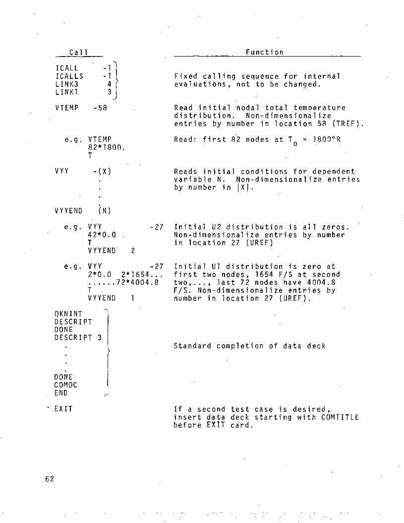
Call Functi on
ICALLICALLSLINKSLINK1
VTEMP
-T-143J
-58
e.g. VTEMP82*1800,T
VYY -(X)
Fixed c a l l i n g sequence for internalevaluations, not to be changed.
Read i n i t i a l nodal total temoeraturedistribution. Non-dimensionalizeentries by number in location 58 (TREF)
Read: first 82 nodes at T = 1800°R
Reads i n i t i a l conditions for dependentv a r i a b l e N. Non-dimensionalize entriesby number in I X I.
VYYEND (N)
e.g. VYY -2742*0.0 .TVYYEND 2
e.g. VYY -272*0.0 2*1654...
72*4004.8TVYYEND 1
QKNINTDESCRIPTDONEDESCRIPT 3
DONECOMOCEND
- EXIT
I n i t i a l U2 d istribution is all zerosNon-dimensionalize entries by numberin location 27 (UREF)
I n i t i a l 111 distribution is zero atfirst two nodes, 1654 F/S at secondtwo,..., last 72 nodes have 4004.8F/S. Non-dimensionalize entries bynumber in location 27 (UREF).
Standard completion of data deck
If a secondinsert databefore EXIT
test case is desired,deck starting with COMTITLEcard.
62

Listed in Table 9 are the changes to the Mach 5 test casedata deck required to establish the three-dimensional virtualsource data deck. The complete listing of the latter is includedas Appendix B. The following explains the alterations with.respect to input phase and the line numbers in Table 9.
InputPhase
I
II
Line No,
12
78
Descri ption
Title card for output cover pageReference condition and control parametersfor combustion calculations using fivedependent variables
Form non-uniform discretization, using 11node rows * 6 node columns, producing 100finite elements
III Title card to head each output callDetailed problem description
IV Entry locations of longitudinal pressuredistribution (constant)66 nodes have uniform stagnation temperatureInitial Ul distribution
Initial 1)2Initial 02of virtualInitial N2Initial H2
distributiondi stri but ionsourcedi stri butiondistri but ion
is zeroref1ects 1 ocation
Hence* establishing the data deck for a m u l t i p l e dependent vari-able, three-dimensional problem using.a. non-uniform finite ele-ment discretization is readily accomplished. In this case, onlyforty data card changes were required, using the two-dimensionalMach 5 data deck as a master deck.
63
cr.
OJr—
JQro
1—
:o
i—
_j—^21*— iCO
Lul
^-^O£^DOCO
~;^^— '1 —D_*~H
^
Lu
^£C_)O
9-
CDi~CO
CD
«=C* -O
^^
LU
CD
•=c^~Q
DA
RY
R
EG
ION
F
LO
W
2
sCO
cz1_t-o
LUQC
1
z0
OOZu.!_!
D
LULUCC.X
oc
u.
LU00<(.J
y/
<->
LU
O
O
oo
0,
KO
UM
P=
0
= l
r
=.0
03
33
33
33
,
u >- -^QC O LLU, 10 LU•- Z a:
•.0.
roroin
•• •• II
II II Zoo x >—< O U.O^5 O^*^ Z ^"
^ (Mu> ^ r^II r\J rviZ ll njZ x n; VO LL0 > ZLL O. • —z z - o
OJ
UJ
UJ
2
O
oII
OOCLLU
O•• o
o — •
» o inO "-1 *M
« II (Min i—II OCa < in-J t- QCUJ CO •• Oo > o t-
o <ro •— •rO Zro O Oro in Zro -< LUro -oro |O •* QC0 0
•• o o <o n o oc-J UJ t-i UJ• -J 51
o < r>u o in zD oo cxj |*- > —< UJ
o•• o
ro ro zroro •• »ro O roro Q xm — .J2 zO LU0 U UJ. in i
O t~» II LL
O LU rv cc.• _l
O < » ooII 0 0 |-C oo 0 z
z:LU
Ln ry
Z
O0
0inOJ
o
»oo
inr-*>^
rj*1
»oo»^
vnr\j^^
o> rvjx
•>O z" LL.'
LU
UT*i H—
U-
£T
r-oo
^ ^~o z-- UJ
LUU> CC
Z
LU UJO Uof a:
5 cU, CO 00LUCt _l _J_j <r <II 3 ^
>- HCO QC QC
UJ •— —-1 > ><I •U 1 1
z z>• 0 O
1 ta* ^H
X O OUJ LU
LU OC QCOZ >- VLU OC OCI < «
«. o Cu. z z
QC a o-J CO CC
>• o oCO ^ Z
»-^ »— 1D H- »-II 1 LJ LJrv) < <M LL LL'-j ct ay i iof <r <.0 Z Zz o o
w* *^i/> co (/;Z Z ZX UJ UJ^ s: y
o c oo
11 1 liJ^ UJ tL-
*• w c^>« C X X
Z »- K
•-J LU LU'l/l v/ t^-
-" C CJ U
-i (_.' 0
X Xo <->
-*Q ^LU — 'a a: voLU <r iQ LU O— Ct Zoo K- >-Z ooO <IO QC CO
— <!z: < zLU—t (_) 00CD t—4 DCO Z UJCC 0 0CL 00 O
QC QC. UJ
— a uj> D UJQC OO 00t- ••^^ f Z!_ o
r o —LU K t-X Z ^O i— i LU
-)a: z zZ3 O •-^— * »— 'OC t- _JCC LJ UJ•— UJ 3
»- z13 *-* ~O1 LUUJ (VI -)
x rX <*- LU QC•- oo (_;"JE QC OO
UJar. > u-LU 00 C1- ZCO < O> oc "iOO K- t—
oooc oo i»
< Z UJ*v LU Ktx oo o
^ QC OC^1 CL Tx LU x~ OC 0
*0mJ-
• r\ir roLU — «_ J 1 UJCD QC (_JO O «oc _ia < a
I/O LUoo < a:— zX O1 — II-
<U. D t-o z a.
< LU> z: oQ ZD 00 Ot- - Ooo cC
LU UJ-J 00 <_>< 3 a^* OZ Z 0UJ fc- COy, , .OC LU <ILU CO ZJa. w. H-x oc ct •LU O — D
00 > _)QC. UJ UJLJ Q O "-•U- Z LL
- *— OO 3Cr- r> oo> c _i— 1 LU O U_•• >• LU
*< O H- Zr- —i cc c«*• o. < •—*D 51 ^~ "I uj oo o
0 LUZ — 1 UJ ~3*- LU cc. z
O «J *-< c00 y 00 ct< z <z uj cr uj
O *•• Zd Z >-Z UJ *S X<T t t 1 1 :
— " cc o a.
a- r> < cfH I- U O
UJat.• u.oo oooo a.UJCC. UJa _i
CDQC <O t-U.
UJ U>_j a:CD ^>< ^i ^J
Ui— a:x a.
• •O roO IT^^ ^J •
ro ro\f\ c? CD# • in
O ro <Q * «
0 --
rororsj•
«•>r
ooPO
roro<NI•
*>!•
O
O
*IM
rororg•
*
O
CJ^ ro ^^ ^^( u^ r C^1 &
r- aa aj V ir O --1-1 •-! — i -j — i rsj CM« « • « • # * « • • »
O O O O t M P v i f M r v j t M o r r ;<G m in in r*- r*~ p - r r . r**i•£> ur* in in rvj rsj rvj r\j r\j o ^
# » * * » * » * # ^ J **i>jrMCNj«\(r \ |cNjr\ iJ jsoao
JJ 0
• 0* »>*• >*•ro ro
0 O.
0 -•» «r\i rsj
^»^O O
• o* «•f ~f
0 0
O -H
* *•rvj rvi
f~%o oIs- •. b
•» *
0 0
.^H
rvj Sj
r^vO Of*» •• o
OO 00
<u^^ CD V C? ^ ^^ fO ^ tf^ ^^ ^~^ - . , — t — r f C N j i ^ r x j r s j o o c s j o u r x j ro <n ro
64

CONCLUDING REMARKS
This report documents the theoretical foundation and themechanical structure of the Three-Dim,ens ional Boundary RegionVariant of the COMOC computer program system. A unified efforthas been made to generate a computational capability that can beaddressed to a wide range of problems i n v o l v i n g comnlex three-dimensional flow fields without requiring undue mathematicalprowess on the part of the user. The success of this tyoe ofventure can only be measured by the degree to which these goalsare approached or attained. As with any large computer orogram,it has been debugged to the extent of the specific problemsalready explored. Hopefully, if bugs remain, they are not ofsuch a d e b i l i t a t i n g nature as to severely l i m i t the usefulnessof the program. In this regard, it is suggested that the poten-tial user first experiment with a few problems whose solutioncharacter is known, in order to attest to the program's perfor-mance for a particular problem class.
65
REFERENCES
1. Orzechowski, 0. A. and Baker, A. J., "COMOC: Three-Dimen-sional Boundary Region Variant, Programmer's Manual," NASACR-132449, 1974.
2. Baker, A. J., "Finite Element Computational Theory forThree-Dimensional Boundary Layer Flow," AIAA Paper 72-108,1972.
3. Baker, A. J., "Finite Element Solution Algorithm for Vis-cous Incompressible Fluid Dynamics," Int. J. Num. Meth.Engr. , 6., 1 , 1973, 89-101 .
4. Baker, A. J., "A Finite Element Solution Algorithm for theNavier-Stokes Equations," NASA CR-2391 , 1973.
5. Bauer, A. M. and Baker, A. J., "COMOC: Thermal AnalysisVariant, User's Manual," NASA CR-130148, 1972.
6. Orzechowski, J. A., Manhardt, P. D. and Baker, A. J., "COMOC:Two-Dimensional Navier-Stokes Variant, User's Manual," BellAerospace Report D9198-954001, 1973.
7. Vincenti, W. G. and Kruger, C. H., Jr., Introduction toPhysical Gas Dynamics, Wiley, New York, 1965.
8. Zienkiewicz, 0. C., The Finite Element Method in EngineeringScience. McGraw-Hill, London, 1971.
9. Nigro, B. J., "The Derivation of Optimally Stable K-Stage,One-Step E x p l i c i t Numerical Integration Methods (K = 1, 2,3)," Bell Aerospace Report TCTN-1008, 1970.
10. Lomax, H., "On the Construction of Hig h l y Stable, E x p l i c i t ,Numerical Methods for Integrating Coupled Ordinary Differ-ential Equations with Parasitic Eiqenvalues," NASA TND-4547,1968.
11. Nigro, B. J., "The Derivation of Optimally Stable and Accu-rate, 3-Stage, 1-Step, E x p l i c i t , Numerical IntegrationMethods," Bell Aerospace Report TCTN-1010, 1971.
12. Mascitti, V. R., "A S i m p l i f i e d E q u i l i b r i u m Hydrocarbon-AirCombustion Gas Model for Convenient Use in Air-BreathingEngine Cycle Computer Programs," NASA L-5825.
13. S c h l i c h t i n g , H., Boundary Layer Theory, McGraw-Hill, NewYork, 1960.
66
14. Strang, W. G. and Fix, G. J., An Analysis of the FiniteElement Method, Prentice H a l l , New Jersey, 1973.
15. Baker, A. J. and Zelazny, S. W., "Predictions in Environ-mental Hydrodynamics Using the Finite Element Method,"AIAA Paper 74-7, 1974.
16. Fischer, H. B., "Longitudinal Dispersion and TurbulentMixing in Open Channel Flow," Annual Rev. Flu. Mech., 5_,1973, 59-78.
17. Jobson, H. E. and Sayre, W. W., J. Hyd. Div., Proceedingsof ASCE, 96, 1970, 703-24.
18. Fischer, H. B., "The Effect of Bends on Dispersion inStreams," Water Resources Research, 5., 2, 1969, 496-506.
19. Patankar, S..V. and Spalding, D. B., Heat and Mass Transferin Boundary Layers, Intertext Books, 1970.
20. Christian, J. W., Hankey, W. L. and Petty, J. S., "SimilarSolutions, of the Attached and Separated Compressible Lami-nar Boundary Layer with Heat Transfer and Pressure Gradient,"ARL-70-0023, 1970.
21. Becker, J. V. and Kirkham, F. S., "Hypersonic Transports,"Pap.er No. 25, NASA SP-292, 1971.
22. Bushnell , D., "Hypersonic Airplane Aerodynamic Technology,"Paper No. 5, NASA SP-292, 1971.
23. Rog-e-r.s^ ;-R. -C. , "A Study of the M i x i n g of Hydrogen InjectedNor.mal :.to a Supersonic Airstream," NASA TND-6114, 1971.
24. Rogers, R. C., "Mixing of Hydrogen Injected From M u l t i p l eInjectors Normal to. a Supersonic Airstream," NASA TND-6476,1971.
25. Baker, A. J. and Zelazny, S. W., "A Theoretical Study ofMixing Downstream of Transverse Injection into a SupersonicBoundary Layer," NASA CR-112254, 1972.
26. van Driest, E. R., "On Turbulent Flow Near a Wall," J.Aero. Sci., 23_, 11, 1956, 1007-1011.
27. Hinze, J. 0., Turbulence, McGraw-Hill, 1959.
28. B i l l i g , F. S., Orth, R. C. and Lasky, M., "A UnifiedAnalysis of Gaseous Jet Penetration," AIAA J., 9_, 6, 1971,1048-1057.
67

APPENDIX A
DATA DECK LISTING FOR MACH 5TWO-DIMENSIONAL FLOW CHECK CASE
FEBLCOMTITLE
CHECK CASE,TWO DIMENSIONAL SUPERSONIC FLOW WITH PRESSURE GRADIENTFENAMEENAME01
N£OKN!M = 2,NPVSX=11,
IGAS=OtN SC X= 1,
IFR=0,NSCY=1,
KOUMP=0,
TOP INF=1800. ,TD=0.2,CPA=0.24,XMA=28.ST,YSCALE=1.0,
RFFL=.0132DELP=5.0tCPH=3.445,XMH=2.016,
RENOSNAME02
. UINF=40C4.8,TQ=0.1fV$TART=5 .0 ,TOH=C.O,XSCALE=1 .0 ,
SENDFEOIMNLINK I 1
I 2 1000,T1 2 1000,T1 21, 1 2,T
CHECK C A S E , T W n DIMENSIONAL SUPERSONIC FLCW WITH PRESSURE GRADIENT
TOA=1800.,
SETUP2
21
2 1CCO,
2 1CCC,
REFERENCE ENGLISH-FT ENGLISH-IN M-K-S C-G-S
DONEMPAHA -1
2 22 22 ?2 22 -1752 22 22 22 22 2
HOLIST
VELOCITY.. .DENSITY. .. .TEMPER ATURE
FROZ .SPEC.V I S C O S I T Y . .
162222222
1692
2
HEAT
LOCAL PRF.SSURP
164 163164 163170 174165 2
2 2176 2
177 178168 167
2 22
.FT.... .... .
.LBP/FT3. .. .
.R4NKINE . . . .
.BTU/LBM. ...
.RTL'/LBM-R. .
. L^M/FT-S. . .
.PSF .PSI
. M
.KG/M3.
.KELVIN.. .,
.KJ/KG....,
.KJ/KG-K. ..
.NT-S/12...
.NT/M2 .. . . .
. CM . . . .
.CM/S..
.G/CC..
.N.A...
.N.A...
.N.A...
.POISE.
.TORR..
68

LOCAL SOLUT IONXl/LRFFICNUMB200200200200999200200
6111
ICSAVE124822481247
-I4*410
9738
36
3200200200
36
10012
-1285278334
14
32042482S2
MACH NC. DPDX1 JLBF/FT3)DXl/lREF EPSILON
2CC 27 200 2*272*10 200 58 200 58
<57 2CO 200 30 200 302*38
36 36
134 12265
284 IC248524f 82*8314
MA0
200200
MIX E F F . ( F T A )OX1MIN/LREF
T U,T,hS,RHO,N2,V,CP,HTOT,H2,02»DIFU fPR NO. ,LAM.VISC. tSCT.NO.IOMULT -I
14*2T U,T,HS,RHC,N2fV,CP,HTOT,H2,02tOIFU,PR NO.,LAM.VlSC.iSCT.NO.
OESCRIPT 2Ul/UREF T/TREF H S T A T / H R E F RHO/PHORFF ELEM.N2 M A S . F R A CU2/UREF CPF/CPFREF HTOT/HRFF FLEM.H2 MAS.FRACELEM.02 MAS.FRACEFF.MU/MUREF EFF,,. PRANDTL NO.MU/WUREF EFF.SCHMIDT NO.CCMOCCESCRIPT
.COMOC .CHECK CASE FOR TWO-DIMENSIONAL FLOW WITH PRESSURE GRADIENT,fl C O M P A R A B L E S I M I L A R I T Y SOLUTION HAS BEEN REPORTED BY CHRISTIAN ET AL,««L 703-'p'o?3. "SPECIFIC C A S E CONSIDERED CORRESPONDS TO MACH NO.5 BETA=0.5,S( 0)=q"^'Ab,I'A8ATIC W A L L I . -SCLUTION STARTED AT X=0.10 FT. WITH SIMILARSOLUTIOr.N".PR'OFILE.LAMiiINA1RmLOW WITH V ISCOSITY FROM SUTHERLANDS LAW.ClSCREti/ATION-:SPAN :S rT-HR^EE TIMES INITIAL BOUNDARY LAYER THICKNESS.ISOPNPR.CF'Ttc FL'OV«-WITH TOTAL TEMPERATURE = isoo R.
D C N F '" "Si=/
11*10.05 0.1
2.846 2.464.3494 3.41T •.'."'-! "
I P I N TI
K 3NO"O.tTOM
KI3NOBOTTOM
K B N OBOTTOM
-I41
-40
T XI TABLE FOR PRESSURE
2.2176 2.02 1.857 1.73 1.6178 1.53 1.4451
3 2 .T INTEGRATE Ul,ENTH.,02,N2tH2,U3,U2
DONEFIXES Ul ( V A R I A 3 L E NO. I) ALCNG WALL TO INITIAL VALUE2
DCNFFIXES U2 ( V A R I A B L E NO. 2) ALONG HALL TO INITIAL VALUE4
DONE - .
69

F I X E S-I(CALL
2 5I C A L L S -1
10 6LINK3 4LINK! 3VTEMP
42*1800T I N I T I A L
V Y Y2*0.0 2*865.
2*3992.
H ( V A R I A B L E NO. 4) ALONG W A L L TO INITIAL VALUE
2 2 1 1 2 T
^ 12 5 6 3 TDIMENGEOMFL
-58
TOTAL TEMPERATURE PROFILE-27
2*1654. 2*2373.2*4CC4.2
2 *3 00* .24*4004.8
2*3550. 2*3879.
T INITIALVYYEND 1VYY
2*0.02*253.
T INITIALVYYEND 2VYY
T INITIALVYYEND 8V Y Y
T INITIALVYYEND 10VYY
T INITIALVYYEND 9OKN INTO E S C R I P TOCNEC E S C R I P T 3
REFERENCEREFERENCEEVALUATEDFREESTREAM
Ul PROFILE
-272*2.12 2*20.142*441. 24*45C.
U2 PROFILE
2*53.52 2*83.2 2*109.3 2*165.
42*. 233002 MASS FRACTION' PROFILE
42*.767CN2 MASS FRACTICN PROFILE
42*0.CH2 MASS FRACTION PROFILE
LENGTH,LREFVISCOSITY.LAMINAR VALUEAT RFF. TEMPERATURE.VELOCITY AT XO(=UREF»
43 FT.
STAGNATION TEMPERATURE (CONSTANT , = TREFIFREF.STRFAM DENSITY AT XO(=RHOREF)FREESTRFAM MACH NUMBER AT XOSTATIC PRESSURE AT XCNUMBER OF NODESNUMBER OF FINITE ELEMENTS
DONECOMOCENDEXIT
38275810
1549
-16-14
LBM/FT-SFT/SOEG RLBM/FT3
PSF
70

APPENDIX.B
DATA DECK LISTING FOR VIRTUAL SOURCETHREE-DIMENSIONAL CHECK CASE
FERLCOMTlT lE
COMOC CHECK CASF FOP THREE DIMENSIONAL REACTING BOUNDARY REGION FLOWRENAME
ENAME01IGAS=1,NSCX=1,
IFR=OfNSCY=l,
KOUMP=0,NPVSX=2,
NEIE2=1,6ENDGNAME02
UINF=2272., TGFINF=533.0,T0=0.0, TD=0.10,XSCALE=C.C03333333 , YSCALE=0. 003333333 , VST ART= lOl.Ot
6ENOFEDIMNLINK I 1
1 75 100, 2 50 100. 3 125 IOC. 4 150 100, 5 225 100,T INCREMENTS BETWEEN X3» NCDE-NUMERATOR-DENOMINATOR
1 5 1C, 7 5 1C, 8 125 100, 9 175 100, 10 250 100,T INCREMENTS BETWEEN X2
1 11, I t,T 11 ROWS AND 6 COLUMNS NORMALIZED BY LREF , HENCE X-Y SCALES = LREF
CHECK C A S E , THREE DIMENSIONAL REACTING BOUNDARY REGION - VIRTUAL SOURCE
REFL=.003333333,OELP=5.0, EPS=O.Ol,
SETUP
REFERENCE ENCLISH-FT ENGLISH-IN
•OONEMP*RA
2222222222
-1?222
-17522222
1622222221692
2
164164170165
v 2176
177lee2
2
163163174
222178
1672
M-K-S C-G-S
HOL 1STLENGTHVELOCITYDENSITYTEMPERATURE. . . .ENTHALPYFROZ.SPEC. HEATVISCOSITY .LOCAL PRESSURELOCAL SOLUTION
.FT
.FT/S
.LBM/FT3...
.RANKINE...
.BTLVLBM...
.BTL/LBM-R.
.LBM/FT-S..
.PSFKACH NO.
.IN M
. N.A .M/S
.N.A. KG/M3
.N.A... KELVIN
.N.A........ .KJ/KG
.N.A KJ/KG-K....
.N.A NT-S/M2....
.PSI NT/M2DPDXl (LBF/FT3) MAX. H2 CONC.
.CM
.CM/S
.G/CC
.N.A
.N.A
.N.A
.POISE
.TORRMIX EFF.(ETA)
71

Xl /LREF DXl /LREF EPSILON DXlHIN/LPEfTONUM3200200200200
999200200
611 1
-I4*4310 200
97 20C38 200
36 36
10012 14
200 27 200 2*272*10 200 58
=7 200 200 302*38
3t 36
134 122£5
•200 58 200200 30 200
-1285 320 284 10248278 4248 9246 8248334 2S2 314HS,RHO,N2,V,CP,HTOT,H2,02,01FU,PR-1
NO. ,LAM.VISC..SCT.NO.
RHO/RHQPEF ELEM.N2 MAS.FRACELEM.H2 MAS.FRACELEM.02 MAS.FRACEFF.SCHMIDT NO.
I O S A V E124822481247T U,T
IOMULT14*2T U,T,HS,RHO,N2,V,CP,HTOT,H2,02,01FU ,PR NO. ,LAM.VISC.,SCT.NO.
DESCRIPT 2Ul/UREF T/TREF HSTAT/HREFU2/UREF CPF/CPFREF HTOT/HREFEFF .MU/MUREF EFF. PRANDTL NO.MLVMUPEFCOMOCD E S C R I P T
CHF.CK C A S E , T H R E E DIMENSIONAL R E A C T I N G BOUNDARY REGION - VIRTUAL SOURCE(H2 /02 /A IR S Y S T E M WITH EQUILIBRIUM CHEMISTRY) . PROBLEM CONSIDEREDREPRESENTS T R A N S V E R S E H2 INJECTION INTO A SUPERSONIC AIR S T R E A MC H A R A C T E R I S T I C OF S C R A M J E T FUEL I NJECTI ON, SEE ROGERS N A S A TNC-6U4,1971 AND N A S A TND-6476,1971 FOR E X P E R I M E N T A L STUDY OF THIS PROBLEM.TURBULENCE MODEL EMPLOYED IS DESCRIBED IN USER'S MANUAL N A S A CR-132450,1974.C A L C U L A T I O N S ARE S T A R T E D USING V I R T U A L SOURCE CONCEPT TO REPLACE
FIELD.
FOR PRESSURE
COMPLDONEVX3ST
0.0VPVSX
193.IPINT
IK 6NOROTTOM
K BNOBOTTOM
K6NOBOTTOM
FX NEAR INJECTION FLOW F
100.
193.-14 . 81
FIXES Ul2
FIXES U24
FIXES H
T XI TABLE
T PRE.SSURE
10 c 3
DCNE(VARIABLE NO.
DONE(VARIABLE NO.
30CNE(VARIABLE NO.
TABLE PSF
2 T INTEGRATE Ul ,ENTH. , 02, N2, H2. U3,U2
1) ALONG W A L L TO INITIAL V A L U E
2) ALCNG W A L L TO INITIAL V A L U E
41 ALCNG W A L L TO INITIAL V A L U E
72
KRNOBOTTOM
KPNOROT TOM
KBNOBOTTOM
FIXES9
FIXES10
ICALL2
KALLS10
L INK3L INK IVTEMP
66*=33,T INITIAL
VYY
-I5
-1643
TOTAL
3DONE(VARIABLE
3DCNE(VARIABLE
3DQNE(VARIABLE
2 I I i
12 5 6 I
-58
TEMPERATURE-27
NO. 8) ALONG W A L L TO INITIAL VALUE
NO. 9) ALONG WALL TO INIT IAL VALUE
NO. 10 ALONG W A L L TO INITIAL VALUE
DIM ENGEOMFL
PROFILE
6*0.06*1503.6*1660.2*1550. 4*1159.2*1550. 4*1833.2*1550. 4*1892.2*2272. 4*1942.2*2272. 4*1985.2*2272. 4*2C74.2*2272. 4*2169.6*2272.
T INITIAL Ul PROFILEV Y Y E N D 1VYY -27
66*0.0T INITIAL U2 PROFILE
VVYEND 2V Y Y
13*.233T INITIAL 02
VYYEND 8VYY
18*.767T INITIAL N2
V Y Y E N D 10VYY
13*0.0T INITIAL H2
V Y Y E N D 9OKN INTO E S C R I P T
DONED E S C R I P T 3
REFERENCE LENGTH,LREFRPFFRFNCE V I S C O S I T Y . L A P I N A R VALUEEVALUATED A T REF . TEMPERATURE.FREESTRFf tM VELOCITY A T X C ( = U R E F )S T A G N A T I O N TEMPERATURE ( C O N S T A N T T = T R E F )FREESTREAM DENSITY A T X O ( = R H C R E F )FREESTP.EAM MACH NUMBER AT XOS T A T I C PRESSURE A T X CNUMBER OF NODESNUMBER OF FINITE ELEMENTS
DONE
2*0.0M A S S FRACTION
2*0.0M A S S F R A C T I O N
2*1.0M A S S F R A C T I O N
4*.233PROFILE
4*.767PROFILE
4*0.0PROFILE
2*0.0 4*.233 2*0.0
2*0.0 4*.767 2*0.0
2*1.0 4*0.0 2*1.0
34*.233
34*.767
34*0.0
43 FT.
38 LBM/FT-S27 FT/S58 DEG R10 LBM/FT3
1549 PSF
-16-14
F X I T
73