NASA TM X-3286 NASA TECHNICAL

MEMORANDUM

co Cn ><

I—

TRANSFER-FUNCTION-PARAMETER ESTIMATION

FROM FREQUENCY RESPONSE DATA -

A FORTRAN PROGRAM

Robert C. Seidel

Lewis Research Center

Cleveland, Ohio 44135oUiT!Ok

1* /

NATIONAL AERONAUTICS AND SPACE ADMINISTRATION WASHINGTON, D. C. • SEPTEMBER 1975

https://ntrs.nasa.gov/search.jsp?R=19750024716 2020-05-16T17:18:45+00:00Z

1. Report No. 2. Government Accession No. 3. Recipients Catalog No,

NASA TMX-3286 4. Title and Subtitle 5. Report Date

TRANSFER-FUNCTION-PARAMETER ESTIMATION FROM September 1975 6. Performing Organization Code FREQUENCY RESPONSE DATA - A FORTRAN PROGRAM

7. Author(s) 8. Performing Organization Report No.

Robert C. -Seidel E-8165 10. Work Unit No.

505-05 9. Performing Organization Name and Address

Lewis Research Center11. Contract or Grant No.

National Aeronautics and Space Administration Cleveland, Ohio 44135

13. Type of Report and Period Covered

Technical Memorandum 12. Sponsoring Agency Name and Address

National Aeronautics and Space Administration Washington, D. C. 20546

14. Sponsoring Agency Code

15. Supplementary Notes

16. Abstract

A FORTRAN computer program designed to fit a linear transfer function model to given frequency response magnitude and phase data is presented. A conjugate gradient search is used that mini-mizes the integral of the absolute value of the error squared between the model and the data. The search is constrained to insure model stability. A scaling of the model parameters by their own magnitude aids search convergence. Efficient computer algorithms result in a small and fast program suitable for a minicomputer. A sample problem with different model structures and parameter estimates is reported.

17. Key Words (Suggested by Author(s)) 18. Distribution Statement

Parameter identification Unclassified - unlimited Gradient search STAR Category 61 Frequency domain

19. Security Classif. (of this report) 20. Security Classif. (of this page) 21. No. of Pages 22. Price

Unclassified Unclassified 32 $3. 75

For sale by the National Technical Information Service, Springfield, Virginia 22161

TRANSFER- FUNCTION- PARAMETER ESTIMATION FROM FREQUENCY

RESPONSE DATA - A FORTRAN PROGRAM

by Robert C. Seidel

Lewis Research Center

SUMMARY

A FORTRAN computer program designed to fit a linear transfer function model to given frequency response magnitude and phase data is presented. A conjugate gradient search is used that minimizes the integral of the absolute value of the error squared between the model and the data. The search is constrained to insure model stability. Scaling of the model parameters by their own magnitude aids search convergence. Ef-ficient computer algorithms are used for the calculation of the cost function and gradi-ent and execution of the search. This results in rapid calculations and a small pro-gram size suitable for running on a minicomputer. Search convergence times for different model structures and parameters estimates for a sample problem derived from experimental data are presented.

INTRODUCTION

Frequency response techniques have long been a fundamental tool of system design and testing. One problem often faced is that of fitting a transfer function to given am-plitude and phase data. One of the most commonly used methods for doing this is the Bode plot graphical technique (ref. 1). Analytical techniques (refs. 2 to 4) that fit rational polynomial transfer functions using the digital computer have also been used. In reference 5 the mathematical framework is presented for a gradient search solution which, not being limited to rational polynomials, can handle dead time parameters, but there are no computer programs or practical results presented.

Reported herein is a FORTRAN computer program designed to fit a transfer func-tion to frequency response data. The program has been used to obtain the transfer function models reported in references 6 and 7 for supersonic mixed-compression inlets. Search convergence times for different model structures and parameter estimates for a

sample problem derived from reference 6 data are presented. A scaling rule is incor-porated to improve search convergence, and a constraint is placed in the search to in-sure model stability during the search. Efficient algorithms used for several different calculations result in a faster program with reduced storage requirements.

The program formulation is first presented, including formulation of the cost func-tion, the model transfer function, the gradient calculation, and the techniques for scal-ing and constraining the model parameters. The computer program is discussed, and a sample problem illustration is given. In appendices A to D the report symbols, the computer program, the sample problem computer listing, and the proofs for various algorithms are presented, respectively.

GENERAL PROGRAM FORMULATION

Cost Function

The desired result is to match a model transfer function to given plant magnitude A(w) and phase 0(w) frequency response data over a range of frequencies w. Ex-pressed in the form of a complex number A(w)e', the plant frequency response should be equivalent to the model transfer function G(jw,b) where jw is the Fourier variable and b is a vector of model parameters. A cost function J(b) representing the fit error between the model and the plant data is formulated to be the integral of the absolute value of the error squared between the model and the data.

J(b) = j G(jw,b) - A(w)e 0 1 dw (1)

In the computer program all calculations are in the frequency domain. However, as an interpretation of equation (1), Parseval ts theorem can be used to transform it into the time domain. As shown in reference 5, the result is that the cost function is the integral of the error squared between the plant and model impulse responses.

The equation (1) is a continuous integral and is not suitable for evaluation with a digital computer; it is also not suitable for tabulated frequency response data. If the tabulated data are a sufficiently representative sample of the plant, the integral can be approximated by replacing the integration with a piecewise linear summation (trapezoi-dal rule):

2

Ndj B (w 2 i)

J(b) G(iw,b) - A(w)e -wi) (2) 2 i+1

i=1

where w0 w1, WN + 1 WN , and Nd 2 is the number of data points in the fre- d d

quency response. Equation (2) is not the usual form of the trapezoidal rule. It has been modified to increase the program speed. The steps in obtaining the equation (2) form from the trapezoidal rule are presented in appendix D.

The choice of the frequencies for the tabulated data can be important. The fre-quency interval (w 1 - w_ 1 ) weights the fit error at each frequency of equation (2). If the frequencies are widely spaced, the value of the error at a particular frequency could have a disproportionate effect. In certain cases it might be desired to favor a close fit between the model and the plant over a portion of the frequency range. The error could be purposely weighted to assign a relative importance to the fit as a function of fre-quency. This could be done to reflect uncertainties in the data, for example. The com-putation time increases proportionately with Nd. Therefore, the user may wish to select a limited number of data points to represent the plant. This is the likely case for pulse testing followed by a fast Fourier transform of the data, which produces a large amount of closely spaced frequency response data. The measurement noise on actual systems has not been too favorable for pulse testing to date, however. The single frequency sinusoidal testing, by comparison, concentrates power at each frequency, virtually eliminating serious measurement noise problems.

Model Transfer Function

The model transfer function is assumed to have a linear structure expressed in factored form. This is the general form familiar to Bode plot users. In this form the transfer function G(s, b), where s is the Laplace variable; consists of the product of a number of possibly different parameter factors.

m -n k pq G(s,b) = 1 g(s,b) m = 1, 2,3,4, 6,8 (3a)

The g(s,b) of equation (3a) are the following parameter factors:

c]

g 1 (s,b) = -- + 1 (3b) bik

92 (s,) =b2 (3c)

g3(s,b)=(bk+ (3d)

3 /

2 2sb4k

94(s, b) =-+ + 1 (3e) - b5 b5

-1

96(s, b)

+ 2sb6k

(31) b7 b7

9 8 ( S 9 b) =e 8 (3g)

The factors of equations (3b), (3d), (3e), and (3f) are assumed to be repeatable in equation (3a). The elements of the b vector are the zeros bik, the gain b2, the poles b3k, the quadratic zero damping ratios b4k, the quadratic zero natural frequencies b5 k) the quadratic pole damping ratios b6 k, the quadratic pole natural frequencies b7 k. and the exponential (dead time) b8. The number of g(s,b) factors in the transfer function is the number of parameters in the b vector m minus the number of quad-ratic factors fl q• The exponent of the free s is k 1 . For example, a particular G(s,b), where

b = (b2, b8, b11,b12,b61,b71)

is

b2 e s )8 I" s +1

+ b1 1 )b2 )

G(s,b) =

(4)

( 7

+ 2sb6 1 + )

b71

4

Gradient Calculation

The gradient of J(b) with respect to b is information required by a gradient search to find parameters b that minimize J(b). The gradient can be expressed analytically by differentiating the equation (2) cost function. The result can be expressed in a form that facilitates rapid computation by invoking the following identiy for a complex func-tion E:

(JE 2)' = ( EE*) ? = E(E')* + E'E* = 212e (E(E t )*) (5)

Here, the prime indicates a derivative and the asterisk indicates a complex conjugate. A proof of this identity is presented in appendix D. The gradient of J(b) is

N

IVJ(b) =ie [G(iwb)

jO(wA(w)e VG(jw,b)*(w.1 - w i) (6)

Furthermore, the VG(jw,b) factor can be written to include all the possible combina-tions of factors for G(jw,b) by defining a vector Z(s,b) such that

VG(s,b) = G(s,b)Z(s,b) (7)

By using G(s,b), which is already computed, the expression is computationally effi-cient. The Z(s,b) elements are internal to the computer program which assigns to each parameter the proper form. The details of the Z(s,b) forms are presented in appendix D.

Parameter Scaling

It was soon apparent from initial trials without parameter scaling that many searches would not converge. Gradient search techniques generally require parameter scaling to obtain efficient search convergence. An ideal scaling rule would obtain nearly spherical cost functions (where the cost is more or less equally sensitive to each parameter of b) and would tend to result in rapidly converging searches. The scaling law adopted applies to the specific form of the factored transfer function parameters. A rule of thumb scaling law was incorporated such that parameters tend to have equal in-fluence. This law scales each parameter by its own magnitude. To show this, a new

5

scaled parameter vector p with elements p1 is defined

pi (i1) b i (8)

where the (bj)h is the magnitude of the b vector elements b at the start of each line search. The elements of the scaled gradient J(p) are formed using the chain rule and equation (8):

ap ap, ab '1h -- (9)

The gradient is computed only at the start of each line search. At this time b1 = (bi)h. Thus, the scaled gradient terms are merely the unscaled gradient terms multiplied by their corresponding parameter values.

The p vector does not actually appear in the computer program. To avoid a con-tinual multiplication of the scaling factor times its scaled parameter and gradient, the search subroutine was specialized to handle the actual parameters and the scaled gra-dient.

Normally, a conjugate gradient search is rescaled only after completing a number of line search iterations equal to at least the number of parameters plus one. But re-scaling here is done after each iteration and is a nonstandard modification to the con-jugate algorithm of reference 8. The advantages for the search program are less logic and storage requirements for scaling parameters to their current value. In tests there were no significant differences found in either the number of iterations or convergence accuracy between rescaling every iteration and after the usual number. This is be-lieved to result from the fact that away from the minimum J(b) is likely to be a poor approximation to the theoretically required quadratic b costs and near the minimum scaling changes are small.

Parameter Constraints

Ideally, it would not be necessary to constrain the model parameters for stability as the infinite error cost function boundary separating stable and unstable models would be reflected in the cost function J(b). However, large changes in b during the search may enable a jump across a relatively narrow error boundary. The solution to this problem was to force a sharp step size reduction on parameters trying to cross zero.

Zero is critical because it is the point of instability for factored parameters. A modifi-cation to the gradient search algorithm constrains the parameters to remain the same sign during the search. This is done by assigning to a parameter about to cross zero a small value on the same side of zero. Thus; an initially stable model must remain stable. This action also prevents changes between right and left hand plane zeroes, and it also prevents changes between dead and lead time exponentials.

COMPUTER PROGRAM AND SAMPLE PROBLEM

The FORTRAN IV computer program reported here mechanizes the transfer func-tion parameter identification. The usual procedure to identify experimental plant data consists of entering tabulated plant amplitude A(w) and phase shift O (w ) frequency response data and a trial factored form transfer function. The user also supplies roughly estimated parameter values and a code number to identify them as time con-stants, gains, etc. The program can then be directed to iterate on the supplied param-eter values until it has optimized the fit to the data. The program output contains the optimized parameter values and a number indicative of the fit error J. Additional out-put includes the model frequency response. The computer program will not change the signs of the user supplied parameter values nor will it change the given transfer function structure.

The computer program was written primarily for a conversational (time-sharing) computer, but it could also be run on a batch process computer. The effort to keep down program size and increase program speed was to enable its use on a minicomputer. The basic program was run on an SEL 810-B minicomputer in a nearly on-line identifi-cation implementation. The intent to obtain a small program package has ruled against writing a program with such conveniences as a plotting package, error detection rou-tines, and alternative search routines. The conjugate gradient search was chosen here because of its simplicity and ease in rescaling and constraining the parameters. Other search routines may converge in fewer iterations. But this could be overbalanced by the resulting increase in computing complexity and scaling and constraining problems. It has not been required to test the program on higher order models (greater than 15 parameters), but generally long convergence times are indicated.

There are provisions in the computer program to make it more general. On occa-sions it may be desired to not iterate on known parameters in the model, but to leave them fixed. This can be accomplished in the program through the computer variable JD, which is the number of fixed variables. Another option is helpful for reducing higher order analytical models to lower order models. Known plant transfer functions can be entered (rather than tabulated plant frequency response data) by setting the com-puter variable INST to 5.

7

G(s,b) = 1

[s + - f[ s 12+2s0.262+1 [17. 5(27i) ] 130 (21T )J 130(27T)

(10)

[T(S27)11r__11[700SO(271)+111+11 ] [1o(2) ]

+iir 12 1Ifl I + j [i000(2)j

2s(1) + 1

1000(2 7T)

G(s,b) =+1

1(2 7T) (11)

+ 11

I + [(3. 70)(2iT) [. O)(2iT) ] [(309)(2iT)

hr 12

+1lfl I ] ft(145)(2iT)]

+ 2s(0.265) 1 (145)(27T)

G(s,b) =

5 +1 4. 91)(2ir

(12)

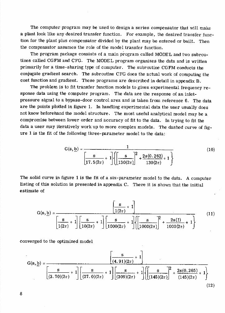
The computer program may be used to design a series compensator that will make a plant look like any desired transfer function. For example, the desired transfer func-tion for the plant plus compensator divided by the plant may be entered or built. Then the compensator assumes the role of the model transfer function.

The program package consists of a main program called MODEL and two subrou-tines called CGFM and CFG. The MODEL program organizes the data and is written primarily for a time-sharing type of computer. The subroutine CGFM conducts the conjugate gradient search. The subroutine CFG does the actual work of computing the cost function and gradient. These programs are described in detail in appendix B.

The problem is to fit transfer function models to given experimental frequency re-sponse data using the computer program. The data are the response of an inlet-pressure signal to a bypass-door control area and is taken from reference 6. The data are the points plotted in figure 1. In handling experimental data the user usually does not know beforehand the model structure. The most useful analytical model may be a compromise between lower order and accuracy of fit to the data. In trying to fit the data a user may iteratively work up to more complex models. The dashed curve of fig-ure 1 is the fit of the following three-parameter model to the data:

The solid curve in figure 1 is the fit of a six-parameter model to the data. A computer listing of this solution is presented in appendix C. There it is shown that the initial estimate of

converged to the optimized model

8

after 93 iterations. The six-parameter fit is visibly better over the frequency range of interest, but both are optimum for their given structure.

The initial parameter estimates can affect the search convergence time and some-times result in detecting a local rather than a global minimum. The convergence times and number of iterations for initial parameter estimates that were off by about a factor of 10 are listed in table I for four different model structures. Convergence times ranged from 24 seconds for the five-parameter model to 1.8 seconds for the two-parameter model (CPU time IBM 360-67 TSS). The fit error J(b) as calculated by the program for various order models are tabulated in table I. The error ranges from 5. 13 for the two-parameter model to 0. 59 for the six-parameter model. The program dis-carded zeroes for models with less than four poles by making them very large. Like-wise, the program discarded a four-pole model by making the fourth pole very large. Two simple poles converging to the same value indicated that a quadratic pole would probably do better.

CONCLUSIONS

A FORTRAN computer program is presented which fits a linear factored form transfer function to given frequency response data. The identification process is often an important first step in system control design. The computer program is based on a conjugate gradient search procedure that minimizes the error between the given frequency-response data and the frequency response of a transfer function that is sup-plied by the user. The user-supplied transfer function consists of a product of terms that can include a gain, an integrator (or differentiator), a dead time, multiple first-order leads and lags, and multiple second-order leads and lags.

The usual procedure for use of the program consists of entering a table of amplitude and phase-shift frequency-response data and a trial, factored form transfer function; the user also supplies roughly estimated parameter values such as time constants, gains, etc. The computer program then iterates on the supplied parameter values until it has optimized the fit to the experimental data; the excellence of this fit is constrained by the form of the user-supplied transfer function. The computer output consists of the optimized parameter values and a number indicative of the fit error. The computer program does not change the signs of the user-supplied parameter values, nor does it change the given transfer-function structure. The user can "build" a transfer function by trying a series of increasingly complex transfer-function structures being guided by the fit errors in a systematic manner as illustrated by the sample problem.

An alternative use is to reduce the complexity of a high-order transfer function that might result from a dynamic analysis. An option is provided in the program for enter-

9

ing the complex transfer function in factored form to take the place of the normal table of frequency response data. The simpler model can then be "built" by the usual pro-cedure until it is a reasonable fit to the more complex model.

The conjugate gradient search routine was chosen for the error function minimiza-tion because of its simplicity and ease in constraining parameters. In the program, scaling the parameters by their own magnitude was demonstrated to result in good search convergence. Constraining the parameters to remain the same sign during the search insures model stability. The use of time and space saving algorithms resulted in a small and fast program. The program as presented is written primarily for a con-versational (time sharing) computer, but it could be run on a batch process computer. The basic program has been run on an SEL 810-B minicomputer as part of a nearly on-line transfer function identification implementation.

Lewis Research Center, National Aeronautics and Space Administration,

Cleveland, Ohio, June 23, 1975, 505-05.

(

10

APPENDiX A

SYMBOLS

A system frequency response magnitude

b parameter vector, m x 1

blk b -

vector kth zero, rad/sec-k

b2 b vector gain parameter, (rad/sec)

b3k b vector kth pole, rad/sec

b4k b vector kth quadratic zero damping

b5 b vector k t h quadratic zero natural frequency, rad/sec

b6k b vector kth quadratic pole damping

b7 b vector kth quadratic pole natural frequency, rad/sec

b8 b vector exponential (dead time), sec

C real variable

d real variable

E complex function, E = c + jd

f real function

fi f(x)

G model transfer function

g transfer function factored parameter factor

J cost function

j imaginary number, Pi jw Fourier transform variable, rad/sec

k1 integer, exponent of free s's in model

m integer, number of elements in b vector

Nd integer, number of frequency points in numerical integration

nq integer, number of quadratic factors

p transformed parameter vector, m x 1

s Laplace variable, sec

11

w frequency, rad/sec

w frequency at tth data point, rad/sec

x1 variable at tth data point

Z partial product in gradient vector, m x 1

9 system frequency response phase, deg

Superscripts:

derivative

* complex conjugate

T transpose

Subscripts:

( )h value at start of iteration

1th element

th factored parameter factor

M type of factored parameter factor

12

APPENDIX B

COMPUTER PROGRAM

The FORTRAN computer program package for transfer function parameter identifi-cation consists of the main program MODEL, subroutine CFG to calculate the cost func-tion and gradient, and subroutine CGFM to conduct the conjugate gradient search. Sym-bols used in the programs are defined separately for each program. The programs are dimensioned for a Nd frequency point maximum of 50 and m model parameter maxi-mum of 15. The vectors dimensioned for N are AMP, PHA, and PLANT. The vectors dimensioned for m are B, G, ID, and Z. The vector H is dimensioned 2m and the vector W is dimensioned Nd + 1.

Program MODEL

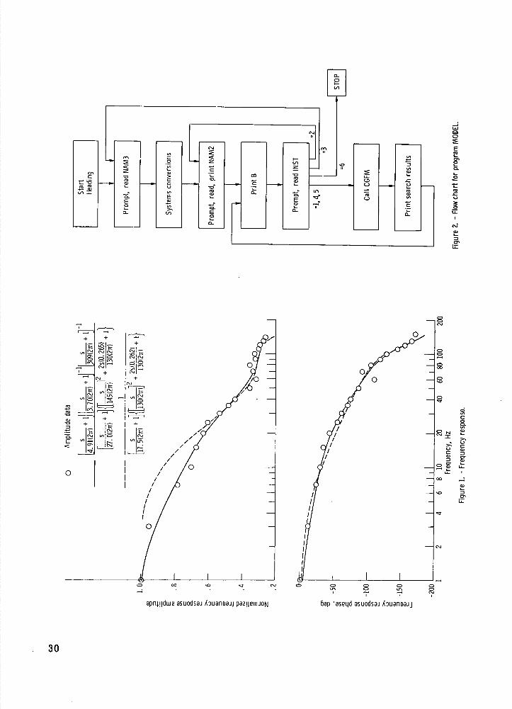
The program MODEL handles the data and converts system frequency response data to complex numbers. The computer variables in the program are defined in the section Program MODEL Variable List. A flow chart for the program MODEL is presented in figure 2.

The program starts by printing a heading referencing the namelist variables and variable codes. Then the program prompts for NAM3 namelist data. The namelist variables are entered according to the rules for entering FORTRAN namelist data. The NAM3 variables are AMP, ND, PHA, W, and KPR. The program prints the NAM3 variables if KPR = 1 and then prompts for NAM2 namelist data. The NAM2 variables are B, Ki, ID, LIMIT, N, and JD. Then the NAM2 variables are printed and a prompt for the INST variable is printed.

The INST variable is entered in Ii format. The INST code values are 1, 2 1 3, 41 5, and 6. Making INST = 1 causes a search for the optimum parameters. After the search results are printed, another INST prompt is issued. Making INST = 2 returns the program to request NAM2. Making INST = 3 returns the program to request NAM3. Making INST = 4 causes the model response to be printed. The frequency is printed under W, the model frequency response amplitude under AMP, and phase under PHA. Then the zero iteration search results are printed and another INST prompt is issued. Making INST = 5 is the same as making INST = 4 except that the PLANT complex num-bers are set equal to the model. This option is used to save entering AMP and PHA data and to build an analytical model for the system. Making INST = 6 stops the pro-gram.

The frequencies W are input in radians, but they may also be input in hertz if the

13

B vector is appropriately scaled by 2ff (see B vector in Program MODEL Variable list).

The following is a FORTRAN listing for the program MODEL 1:

C PROGRAM MODEL FOR TRANSFER FUNCTION IDENTIFICATION DIMENSION B(15),G(15), ID(15),AMP(50),PHA(50),W(51),H(30) COMPLEX PLANT(50) EXTERNAL CFG LOGICAL KG COMMON/ I DTF4/PLANT,W, ID, Ki, I UST, tID ; KNT, NP C01414ON/FI4C/KOUNT, KG NAMEL I ST /NAM3/W, AMP, PIIA, ND, KPR /NAM2 Ill MIT, N, Ki, B, I D, JO WRITE(6 110)

110 FORMAT(1 NAM3=(W, AMP, PHA, ND, KPR)1,' 1IAM2=(B, ID,Kl,LIMIT,N,JD)',/-2,' ID=(1Z;2 = G;3P;4,5CZD,CZ14;6,7CPD,CPW;8=DT)',/-3, ' I NST= ( i=SEARCI, 2=NAt'12, 3 = NAM3, 4= PR I NT, 5 = PLANT=MODE L, 6 = - 4STOP)',/,' IER=(O=COUV,i=NOT CONV,2=ERROR)' )

10 WRITE (6,180) 180 FORMAT(' NAM3?1)

READ (5,NAM3) I F(KPR.EQ.i) WRITE(6, 310)

310 FORMAT(6H PLANT,/,RX,1NI,i4X,3I1AMp,iiX,3HpfIA) 120 FORMAT(1P3E15.5)

DO 20 J=1,ND IF(KPR.EQ.1) WRITEt6,120 wJ,AMP(J),FuA(J) TIIETA=PHA(J)*. 017453292

20 PLANT(J)=A1IP(J)*CEXP(CMPLX(O.,TIIETA)) W(ND+1)=W(ND)

30 WRITE (6,181) 181 FORMAT( ' NAM2?' )

READ (5,NAM2) N P = +J D WRITE(6,130) Ll4IT,N,K1,JD,(Io(J),J=i,Np)

130 FORMAT.(' LIMIT,N,K1,JD = ',413,' ID=',1513) GO TO 87

777 WRITE (6,182) 182 FORMAT(' INST?')

READ (5,140) INST 140 FORMAT (Ii)

GO TO (40,30,10,50,45,1000), INST 45 WRITE(6,145) 145 FORMAT(' PLANT SET EQUAL TO MODEL') 50 WRITE(6,160) 160 FORMAT(61-1 MODEL,!, RX, 111W, 14X, 3HAMP, lix, 3IIPHA) 40 SIZE=.i

EPS=1.E_5 I TER=L I MI T*( 1-I NST/4) KNT=0 CALL CGFM(CFG,N,B,F,G, SIZE, EPS,I TER, IER,H) WRITE(6,15O) F,IER,KOIJUT,KNT,SIZE

150 FORMAT(' F=', 1PE16. 7,' I ER=',12, ' KOUNT, KNT, SI ZE=', - 1 13, 14, 1PE10.3)

87 WRITE (8,151) (B(J),J=i,Np) 151 FORMAT(' B=',1P8E11.10

dash at end of a line signals continuation card follows.

14

GO TO 777

1000 STOP END

Program Model Variable List

AMP system frequency response magnitude A(w), vector (input variable)

B model parameter b, vector (input variable). Damping ratios must immedi-ately precede their natural frequency terms. Constant (JD) parameters must follow last.

CFG subroutine (declared external in model program) which computes the cost function and gradient

EPS parameter change defining search convergence, e.g., 10

F F J(b), cost function

G cost function (scaled) gradient, vector

H storage, vector

ID integer vector that identifies corresponding parameter in B as to type (input variable): 1 = zero, 2 = gain, 3 = pole, 4 = complex zero damping, 5 = complex zero natural frequency, 6 = complex pole damping, 7 = complex pole natural frequency, 8 = dead time

IER search convergence parameter: 0 = search convergence (SIZE reduced to EPS or less within LIMIT iterations), 1 search not converged, 2 = prob-able error occurred

INST

ITER

J

JD

KG

KNT

branching instruction parameter (input variable): 1 = search for optimum, 2 = return to NAM2 namelist, 3 return to NAM3 namelist, 4 = print fre-quency and model frequency response amplitude and phase, 5 = set con-verted system PLANT frequency responses equal to model values and print, 6 = stop

set equal to LIMIT except for the INST = 4 or 5 in which case ITER 0

index of element in vector

number of noniterative constant parameters in model (input variable)

logical variable . TRUE. means compute gradient

count of cost function evaluations

KOUNT count of line search iterations

15

KPR if equal to 1 causes NAM3 variables to be printed (input variable)

Ki exponent of free s in model (input variable)

LIMIT maximum number of iterations (input variable)

N number of iterative parameters of B in model (input variable)

ND number of frequency points over which integration is performed Nd

NP total number, iterative plus constant, of model parameters, NP = N + JD

PHA system frequency response phase 9(w), in deg vector (input variable)

PLANT converted system response to equivalent complex numbers vector

SIZE parameter step size; e. g., set to 0. 1 at start of search

THETA scratch variable for radian phase

W radian frequency w, vector (input variable); can be input in hertz instead of radians but then the units of parameters in B may change. (The B parameters with ID numbers of 1, 3, 5, and 7 need to be divided by 27r tc obtain their corresponding value in hertz, a B with an ID = 8 needs to be multiplied by 27r, and B's with ID = 2, 4, and 6 are not affected)

Subroutine CFG (N, B, F, G)

The purpose of this subroutine is to compute the cost function and gradient. The gradient G is the scaled gradient VJ(p). The unsealed gradient for other search pro-grams could be obtained by dividing each term in G by the corresponding parameter in B.

The CFG variables are defined in the CFG Variable List. Those variables carried over in the common block and subroutine call are labeled the same as those described in the program MODEL and are not repeated again. Figure 3 is a flow chart of CFG.

FORTRAN Listing for Subroutine CFG

SUBROUTINE CFG(N,B,F,G) IIMENSION B(1),G(1), ID(lS),W(51) COMPLEX PLAF'IT(50),Z(15),S,ST,GM,E LOGICAL KG COMMON/ I DTN/PLANT,w, I D, Ki, I NST, ND, KNI, NP COMMON/FMC/KOUNT, KG KNTKNT+1 DO 30 J=1,N

16

30 G(I)=0. WS=W( 1) F=0. DO 100 J=1, ND S=CMPLX(0.,J(J)) GM = S * * K 1 DO 8 K=1, NP I DK= I D( K) GO TO ( 1, 3, 1, 2, 8, 2, 8, 14), IDK G11=Gli*(S/B(K)+l.)**(2-IDK) IF(KG) Z(K)=S/(S+B(K))*(FLOAT( IDK)-2.) GO TO 8

2 ST=(S/B(K+1))**2+2.*S*B(K)/B(K+1)+1. GM=Gli*ST**(5-I OK) IF(.NOT.KG) GO TO 8 Z( K) = 2 . * 5 * 3( K) /( B( K+1)*ST) *( 5. -FLOAT( I OK)) Z( K+1)=-Z( K) *( 1. BC K) *B( K1) )) GO TO 8

3 GM=GM*B(K) Z(K)=CMPLX(1.,0.) GO TO 8 Gtl=GM*CEXP( -S*B( K)) Z( K)=-S*B( K)

8 CONTINUE E=GM-PLANT(J) F=F+(W(J+1)-WS)*REAL(E*CON)G(E)) IF(. NOT. KG ) GO TO 100 ST=('I(J+1) -WS) *E*cO1JG(GM) DO 80 K=1,N

80 G(K)=G(K)+REAL(ST*COlJJG(Z(K))) IF(INST. EQ. 1) GO TO 100 AM=CABS(GM) DEG=ATAH2(AIMAG(Gti),REAL(GM))*57.295780 WRITE(6,120) W(J), AM, DEG

120 FORMAT (1P3E15.5 ) I F( I ST. Efl. 5) PLANT(J)=Gtl

100 WS=W(J) RETURN END

Subroutine CFG Variable List

AM I G(Jw,b)

DEG /G(jw,b), deg

E error between model and data

GM partial product becomes G(s,b)

IDK ID(K) value

J frequency index

K parameter index

17

S S

ST temporary value

WS saved W value

Z partial product in model gradient, vector

Subroutine CGFM (CFG, N, B, F, G, SIZE, EPS, ITER, IER, H)

The purpose of subroutine CGFM is to perform the conjugate gradient search func-tion minimization. Several nonstandard modifications relative to the conjugate gradient search described in reference 8 exist in the CGFM subroutine. The gradient is the scaled gradient VJ(p) and every iteration updated b parameters change the scaled co-ordinate system. Another nonstandard modification to the search is that the signs of the parameters b are not allowed to change during the search'.

The minimum for each line search is found by either doubling or taking one third of the parameter values. The process is continued until the minimum cost is known to be bracketed. Then the minimum point is obtained from the minimum of a quadratic curve fit to three points. The gradient is not used in this process. To increase the program speed, there is logic to signal whether the gradient is needed; if not, only the cost function value is required of the CFG subroutine.

The CGFM program variables are defined in the CGFM program variable list. Variables carried over in the common block and subroutine call are labeled the same as those described in the main program and are not repeated again. Figure 4 is a flow chart of CGFM.

FORTRAN Listing of Subroutine CGFM

SUBROUTINE CGFM(CFG,N,B,F,G,SIZE,EPSITER,IER,H) DIMENSION B( l),H( l),G(1) LOGICAL KG COMMON/ FMC/ KOIJNT, KG

C INITIALIZATIONS KOIJNT=O STEP=2. I ER=-5

5 BETA-0. NCY C= 0

15 K=0 DO 20 J=1,N

20 H(J)=B(J) KG=.TRUE. CALL CFG(NB,F,(-,)

18

C TEST FOR STOPPING SEARCH IF(KOUNT.GE .ITER) IER=1 I F(SIZE.LT .EPS) IER=0

40 IF(IER.GT .-2) RETURN C COMPUTE PAST GRADIENT WEIGHTING

TSflR=0. DO 50 J=1,N

50 TSflR=TSQR+G(J)**2 IF(NCYC.EQ.,cJ) GO TO 60 BETA=TSQR/TSAVE

60 SCALE=O. DO 70 J=1,N ju= j +ri H(JN)=—G(J)+BETA*FJ(J1)

70 SCALE=SCALE+ABS(FI(Ju)) IF(SCALE.GT.O.) GO TO 80 I ER=0 GO TO 40

80 SCALE=SIZE/SCALE TSAVE=TSQR UCYC=NCYC+1 F S S= F L=1

C UPDATE B'S 100 DO 110 J=1,N

J N = J + J 110 B(J)=H(J)*Afl5(1.+SCALE*F(JFj))

FS=F KG=.FALSE. CALL CFG(NB,F,G)

C LOGIC CHANGES LINE SEARCH STEP SIZE OR CONCLUDES SEARCH IF(K.GT.0) GO TO 120 IF(F.LT.FS) GO TO 130 IF(L.GT.1) GO TO 140 GO TO 150

120 IF(F.LT.FSS) GO TO 140 GO TO 160

130 SCASV = SCALE L= L+1 SCALE= SCALE*STEp FSS=FS IF(L.LT.15) GO TO 100 I ER=2 GO TO 40

C FIT QUADRATIC CURVE TO 3 PIS. BRACKETING LINE SEARCH MIN. 140 DO 148 J=1,14

J=J+4 Ri=I1(J) R2=II(J)*ABS(1.+SCA3V*,(JU)) R3=B(J) IF(L.GT.3) R1=R1+(R2—R1)/STEP X1=( FSS—FS)*(R1—R3) X2 = (FSS—F)*(R2 —Ri) IF ( AB S(R2 — R3).GT.E p S/4) GO TO 147 IF(L.GT.1) 8(J)=R2 GO TO 148

147 148 IF(B(J)*H(J).LE.Q.) B(J)=—.1*B(J)+EpS*R3

19

C UPDATE SEARCH VARIABLES SIZE=SIZE*(FLOAT(L)+2.)/14. KOUt4T KOUrIT +1 IF(NCYC.GT .N) GO TO 5 GO TO 15

150 SCASV SCALE SCALE= SCALE/(1.+STEP) K= K+1 SIZE= SIZE/(1.+STEP) GO TO 100

160 SIZE = SIZE/(1.+STEP) DO 180 J=1.,,N

180 B(J)=H(J) GO TO 5 END

CGFM Program Variable List

BETA conjugate direction weighting

FS saved F

FSS saved F'S

J parameter index

JN J + N

K indicator for step size reductions

L number step size increases within iteration

NCYC number of iterations before restarting conjugate search

Rl,R2,R3 terms in quadratic curve fit

SCALE step size scale factor

SCASV saved SCALE

STEP step size

TSAVE saved TSQR

TSQR squared gradient terms sum

Xl, X2 partial product

APPENDIX C

SAMPLE PROBLEM LISTING

The computer listing for the optimization of a six-parameter model is presented:

1 NAM 3= (W, AMP, PHA, ND, KPR) 2 UAM2 = (B, ID,K1, WAIT, U,JD) 3 1 D( 1Z; 2 = G; 3P; 4, 5CZ0, CZW; 6, 7 = CPD, CPW; 8=DT) 4 INST=(1=SEARCII,2=NAM2,3=NAM3,4=PRINT,5PLAt.ITMODEL,6STOP) 5 I ER=(0 = CONV, 1 = NOT C014V, 2=ERROR) 6 NAM3? 7 &nam3 w = 1,3,7,1O,15,20,25,30,35,L40, 50,60, 70,80,90,100, 110,120,130, 140, 8 amp=1,.95,.77,.7,.67,.63,.6,.53.4844353l333S23232g 9 .27, .26, pha=-2, -13, -24, -31, -35, -44, -57, -62, -71, 75, 87, -110, -92, -105,

10 ll9,128,-145,-156,-156,-172,nd20,kpr0 &end 11 NAM2? 12 &nam2 b = l,l,1O,l000,1,1000, id = 1,3,3,3,6,7,k1=0,ljmjt=200 n=6 jd=O &end 13 LItIIT,N,K1,JD=200 6 0 0 10= 1 3 3 3 6 7 14 B= 1.0000E 00 1.0000E 00 1.0000E 01 1.0000E 03 1.0000E 00 1.0000E 03 15 lUST? 161 17 Fu 5.8507025E-01 IER= 0 KOUNT,KNT,SIZE= 93 417 2.868E-06 18 B= 4.9144E 00 3.6908E 00 2.6970E 01 3.0934E 02 2.6459E-01 1.4546E 02 19 lUST? 206

CIICRW400 TERMINATED: STOP

The listing shows the plant data entered in NAM3 namelist, a model built in NAM2 namelist, and a search for the optimum parameters. The line numbers were added for discussion purposes, and program responses are capital letter while user input are lowercase. A line by line discussion of the listing follows:

Lines 1 to 5 - For convenience the program listing of the NAM3 and NAM2 variables and the ID, ThTST, and IER variable codes

Line 6 - A program prompt for NAM3 name list data

Lines 7 to 10 - The user entered system NAM3 frequency response data

(The frequencies of W are entered in hertz rather than in radians. This requires associating a conversion factor of 2u with certain parameters of B.

Line 11 - A program prompt for NAM2 name list data

Line 12 - User entered NAM2 namelist data required to build the iterative six-parameter transfer function model (See eq. (11).)

Lines 13 and 14 - Program verification of the NAM2 namelist data

Line 15 - A program prompt for a branching instruction

21

Line 16 - A user input 1 directing the program to search for the optimum parameters

Lines 17 and 18 - Program output of search results (Upon convergence the cost func-tion was reduced to 0. 585 after 93 iterations and 417 cost function evaluations. The optimized parameters are listed in eq. (12).)

Line 19 - Another program prompt for a branching instruction

Line 20 - A user input 6 to stop the program

In the sample problem parameter optimization the KPR variable was not set to 1; therefore, there was no recording of the plant data. The INST variable was not set to 4; therefore, there was no recording of the model frequency response. The following listing shows the output upon recalling the program for the case KPR 1 and INST = 4, but with the NAM3 and NAM2 namelist data otherwise unchanged.

Sample problem plant and model frequency response

NAM 3=( ti, AMP, P /t I Nfl, K PP) NAt42= ( B, ID, Ki, L IMIT, N, J fl) ID=(1=Z; 2=(; 3=P;4, 5=C7fl,C71;6, 7=C',tPW; R=DT) INST=( l=SEARCH, 2=NAM2, 3=NAt3, t4=PRI 'T, 5 = PLA T=l"fl!)E!. , 6-STOP) IER=(0=CONV,1=NflT CONV,2=ERROR) NAM3? &nam3 kpr=i &end

PLANTIII

1.00000E 00 1.00000F 00 3.00000F 00 9.50000E-n1 7.00000E Or) 7.7fl000E-fl1 1.00000E01 7.rl0000E-01 1.50000E 01 .7fl00flE-01 2.00000E 01 6.30000E-01 2.50000E 01 6.00000E-01 3.00000E 01 5.300007_01 3.50000F 01 14.P0000E-fll 14.00000E 01 4.4fl000E-01 5.00000E 01 3.50000c_01 6.00000E 01 .lfl0Ofl-01 7.00000E 01. 3.30nflrI-n1 8.00000E 01 3.50000E-01 9.00000F 01 .2 0000E-01 1.00000E 02 3.20000-01 1.10000E 02 .flOfl0fl-fl1 1.20000E 02 2.90000E-01 1.30000E 02 2.70000E-01 1.40000F 02 2.60000r-01

-2.nOflnflE 00 -1 • nf)oF 01 -2.0fl00E 01 -3. 1.000flF 01 -3.! 01 -t.40fl0F 01 -5.7n00F 01

01 -7.10000E 01 -7.500flfl' 01 -P.70000E 01 -1.10000 (2 -.2flflflfl 01

.. rçt'n 02 -1. 11)0 02 - 1 • 2M0flE 02 -1. 1 50"O r 02 -1.50flflE 02 -1 • 1E000 02 -1.72 t)OOE 02

N AM 2? &nam2 &end

LIMIT,N,K1,JD=200 B= 14.911414E 00 3.6998F I NST? 4

0 0 IP= 1 3 3 3 F 7 00 2.1970E 01 3. fl 034E 02 2.F49-01 1.451tE 02

22

MODELVI

1.00000E 00 9.845fl1E-01 -I.1033F flQ 3.00000E 00 9.0473cn -1.51,638E 01 7.00000E 00 7.R8533E-01 -2.45215E 01 1.00000E 01 7.4027flE-fl1 -3.01572E 01 1.50000E 01 6.775O1E-01 -3.9290RE 01 2.00000E 01 6.21103F-01 -4.7R250F 01 2.50000E 01 5.69208E-Ol -5.55071F 01 3.00000E 01 5.2281QE-01 -6.2350RF 01 3.50000E 01 4.9231QE-01 -6.404F 01 4.00000E 01 4.47492E-01 -7'. L0ti7E 01 5.00000E 01 3.926E-01 -0.38764E 01 6.00000E 01 3.53632-01 -9.246r 01 7.00000E 01 3.26157E-01 -1.01007E 02 8.00000E 01 3.08326E_01 -1.013R7E 02 9.00000E 01 2.07201E-01 -1 18260F 02 1.00000E 02 2.11303E-01 - 1 .2R117E 02 1.10000E 02 2.88359E-01 -1.05fl7E 02 1.20000E 02 2.8462PE-01 -1.52927E 02 1.30000E 02 2.7434E-01 -1.fR52E 02 1.40000E 02 2.52175E-fl1 1.742RflE 02

F = 5.8507025E-01 tER= 1 KOUNT,KNT,SIZF= '0 1 1.IflflE-fl1 B= 4.9144E 00 3.6998E 00 2.697flE 01 3.0 0 3 14E 02 2.6459E-01 1 .4546F 02 INSI?

23

APPENDIX D

TRAPEZOIDAL RULE

The trapezoidal rule for the approximation of an integral is

xi+l xi+l - x f(x) dx

2[f(x+1) + f(xj)]

This leads naturally to the series expression for a piecewise linear summation of trapezoidal areas

t

1 (f 1 + f)(x 1 - xi)

where the notation f(x) is shorted to f1 . Note that for each value of i the series re-quires the two values f1 and f11 . This is reduced to a single value f1 as described next. First, the series is written in expanded form

+ f 1x2 - f2x1 - f1x1 ) + 1 (f3x3 + f2x3 - f3x2 - f2x2 ) +.

2 k x +

Nd Nd 1Nd lxNd - fNdxNd_ 1 - 1Nd- 1 XNd_ 1)

The expansion after cancellation of terms from adjacent lines is

1 (0 + f1x2 - f2x1 - f1x1 ) + 1 (0 + f2x3 - f3x2 - 0) +.

+ (NdxNd + ENd- 1XNd - fNdxNd 1 - o)

A regrouping of the expansion forms the series

24

[ 1 x2 - x 1 ) + f2 (x3 - x 1 ) + f3 (x4 - x2 ) + . . . + fNd(xNd - xN1)]

The series is expressed in the desired form by defining x 0 x1 and xN 1 = XN Thus, d d

N

2 !f(xi )(xi+1 -xii) 4'

1=1

Identity

If E is assumed to be a complex function of two real variables c and d,

E = c + jd

it readily follows that

(E 2 ) ' = [(c + jd)(c - id)]' = (c 2 + d2 ) = 2(cc' + dd')

For another starting point, namely, 2 Re (E (E t)* ), the result is

2 Re (E(E')*) = 2 Re [(c + jd)(c' - jd')] = 2(cc' + dd')

Thus, the two expressions are the same, and

(E 2 ) ' =2 Re (E(E')*)

Gradient

The cost function gradient (eq. (6)) contains the transfer function gradient. The transfer function gradient in equation (7) is the transfer function times a vector Z(s,b).

VG(s,b) = [G (s, b)] [Z (s, b)] (7)

The transfer function G(s,b) is the product of factored parameter factors g(s,b) (eq. (3a) to (3g)). The elements of Z(s,b) are the partial derivatives divided by the

25

corresponding factor. For example, the Z(s,b) element for a bik factor is

a(^'k-_ + I

abik - b1

ss + _+

\blk I ) There are eight structural forms for the Z(s, b) elements corresponding to the eight possible parameter forms. The terms are simple, and there is only a change in sign between corresponding numerator and denominator factor forms.

-s

b12 bik:

k

\blk I

b2:b2

S

2

Wki — + 1 \b3k

b5k b4k:

/2 2s(b4 k (s + +i)

b5

26

/b 2\ -2sj +____'

b5k:b5)

( 5

2s(b4k) b5 +i)

- 2s

b6 b7 k'

/'2 2s(b6k) I + +

\b7k b7

b'Ik:(b7 b7)

+ 2s(b6) +

( 7 2b7k

b8: -s

27

REFERENCES

1. D'Azzo, John J.; Houpis, Constantine H.: Feedback Control System Analysis and Synthesis. McGraw-Hill, 1966.

2. Sanathan, C. K.; Koerner, J.: Transfer Function Synthesis as a Ratio of Two Com-plex Polynomials. IEEE Trans. Auto. Control, vol. AC-8, no. 1, Jan. 1963,

pp. 56-58.

3. Strobel, H.: On a New Method of Determining the Transfer Function By Simultaneous Evaluation of the Real and Imaginary Part of the Frequency Response. Paper 1. F, Proc. 3rd IFAC Congress, Session 1, 1966.

4. Jones, N. B.: New Method for Identification and Synthesis of Linear Systems from Frequency Response Data. Proc. Inst. of Elec. Engs., vol. 117, 1970, pp. 1021- 1025.

5. Hays, James R.; Clements, William C., Jr.; and Harris, Thomas R.: The Fre-quency Domain Evaluation of Mathematical Models for Dynamic Systems. Amer. Inst. Chem. Eng. J., vol. 13, No. 2, 1967, pp. 374-378.

6. Baumbick, Robert J.; Neiner, George H.;' and Cole, Gary L.: Experimental Dy-namic Response of a Two-Dimensional, Mach 2. 7, Mixed-Compression Inlet. NASA TN D-6957 9 1972.

7. Baumbick, Robert J.; et al.: Dynamic Response of Mach 2. 5 Axisymmetric Inlet with 40 Percent Supersonic Internal Area Contraction. NASA TM X-2883 2 1973.

8. Fletcher, R.; and Reeves, C. M.: Function Minimization by Conjugate Gradients. Computer J., vol. 7, No. 2, Jul. 1964, pp. 149-154.

28

0 Cl)

Cl)

z

0

4-I

CD

I I

0

C)

— C9 0

.. 0 0

to C)-4

OD OD

CID C)

z

'-4

+ +1 , I

+

.01'-4

CO I t C) I+ I tO) I

i CSI CII dlo '' vQI Cli

S IC)I I. c i IClI +

.-Icl) + '—IClI 0 LM

Ic\I csil I ciI I i 4 cII

0 +q•jI_.I

+-

+

I I I I

IClII ic)1 l

ICl.i+

I___

cnI:; C9cli

+___ ..L4Li

+

-'

IClI ___ LJ

3I0 I -

Lo

I' '-I 1111 I_I I IC) I I -

1iIC)I I U) Cl)

+ ' +

ItI ___ II '

U)lCO i U)ILC)

IC'.IC) t12I4

IC) t I. L IC

I I '••i I

+ —I + + I_-_

ItI ''-I I eq .01 II

ItI IC% +

U o Cl10C.1I0 0 I' 10 +

l'— Ici I—Ii'-i

lo i.. + Ui +

o I, tiiIO

—I +

Cl U

'0 I Ci

Cd___

I •;;;i tI L I t -

L IItI I 0

Cl)Cl

11)10 ' I_411)10

Cd

I o

1° +

C1)I.l L_J

I+

+

+ -.----- -

+

ICI

rliI lo

+ 1121tI Ci

I I ", j - I

.1.10,01

co ,-i C)

Cl C-

C) to)

-

o I-U;--

01Cl co to CO

Cd 01

co

Cd C)

0

Cl)

29

+

C%J

+ NJ

U, NJ

'N

+

NJ

/ /

/ /

0/

- +1 +

z^

0

NJ

NJ

CD It

QJ

C a 0

1.) 0 C

a-a,

00 -

0)

0' LJ

0

E 0

0.

0

0

U

0 LJ

NJ 0

C, LL

00 '0 NJ CD

- CD I

aP fl l ! I dWe asuodsai Aouanbj paZ!I2WJON

5ap aseqd asuodsa A: )uanbaij

30

= 0 -o

0

0

a,

(

a, =

0 0

0

(0

C,

0

a,

0 U-

NASA-Langley,1975 E8165 31

p.I

t, -

- .--- --L; -• ---- • t-

rp • 1JL

- r-- .

r-

- -

-

AL

mj :

!

--IL

3WJWi :4P

j!i7

..L,_,-.e.. •_;-•-i.& -' f- -

'k ' '.•- - *.J J-1._ L

L L••'&I, Jt-;,..-

N- rlo' j44 •-

Nkr

ST PIQ

r

-r

lip

- WO

"

104, %.1.- 141118^^

Lj

irr -4dI-

p r'•';

'i.LiF. r•-.L :-.- -.- . ! -' - .-•

E

I•rj. •ic-1I.!, ez .• -

r-,-j- r ---'

Jjq JIIJ

. - v ' tr

T1 1Oi jIF

116 y,

FL

ji

Ir

. •-r -:

- I.iJ! 1 1 6 1•.

qL

SW

j J1

POSTAGE AND FEES PAID

-I*- NATIONAL AERONAUTICS AND

SPACE ADMINISTRATION 45,

LLS.MAIL

NATIONAL AERONAUTICS AND SPACE ADMINISTRATION WASHINGTON. D.C. 20546

OFFICIAL BUSINESS PENALTY FOR PRIVATE USE 5300 SPECIAL FOURTH-CLASS RATE

BOOK

If Undeliverable (Section 158 POSTMASTER Postal Manual) DII Not Return

"T/,e aeronautical and space activities of the United States shall be conducted so as to contribute . . to the expansion of human know!-edge of phenomena in the atmosphere and space. The Administration shall provide for the widest practicable and appropriate dissemination of information concerning its activities and the results thereof,"

—NATIONAL AERONAUTICS AND SPACE ACT OF 1958

NASA SCIENTIFIC AND TECHNICAL PUBLICATIONS TECHNICAL REPORTS: Scientific and technical information considered important, complete, and a lasting contribution to existing knowledge.

TECHNICAL NOTES: Information less broad in scope but nevertheless of importance as a contribution to existing knowledge.

TECHNICAL MEMORANDUMS: Information receiving limited distribution because of preliminary data, security classifica-tion, or other reasons. Also includes conference proceedings with either limited or unlimited distribution.

CONTRACTOR REPORTS: Scientific and technical information generated under a NASA contract or grant and considered an important contribution to existing knowledge.

TECHNICAL TRANSLATIONS: laformation published in a foreign language considered to merit NASA distribution in English.

SPECIAL PUBLICATIONS: Information derived from or of value to NASA activities. Publications include final reports of major projects, monographs, data compilations, handbooks, sourcebooks, and special bibliographies.

TECHNOLOGY UTILIZATION PUBLICATIONS: Information on technology used by NASA that may be of particular interest in commercial and other non -aerospace applications. Publications include Tech Briefs, Technology Utilization Reports and Technology Surveys.

Details on the availability of these publications may be obtained from:

SCIENTIFIC AND TECHNICAL INFORMATION OFFICE

NATIONAL AERONAUTICS AND SPACE ADMINISTRATION Washington, D.C. 20546