nash certainty equivalence in large population stochastic...

Nash Certainty Equivalence in Large PopulationStochastic Dynamic Games: Connections with the

Physics of Interacting Particle Systems

Minyi Huang

School of Mathematics and Statistics

Carleton University, Ottawa

With Peter E. Caines , McGill, Montreal

& Roland P. Malhame, Ecole Poly. Montreal

Carleton, Nov. 2007

Huang, Caines, Malhame, 2007 – p.1/33

Brief Historic Background: von Neumann and Morgenstern

� Following the publication of Theory of Games and Economic Behavior by

John von Neumann and Oskar Morgenstern in 1944, Game Theory

was established as a scientific discipline

� Key results: saddle strategies in two-person zero-sum games

“min max = max min”

� Significance: Ground breaking, marking a new era of research

spanning over multi-disciplines

� Limitation: difficult to extend to multi-person situations

� But they guessed that there might exist good methods to deal with

many players


Brief Historic Background: John Nash

� John Nash (1950) Equilibrium points in N-Person Games, PNAS.

� Key notion: Nash equilibrium

� Key results: Existence of equilibrium

� Method: Kakutani’s fixed point theorem

The impact of this brief paper (less than 30 lines) is profound:

� Economics

� Social Sciences (arms control, international relations)

� Evolutionary Biology

� etc.


Brief Historic Background: Prisoner’s Dilemma

A Very Simple Model with a Rich Structure:

� Two criminal suspects were caught by police

� “Accuse" means “accuse the other side"–If A accuse B who

incidentally confesses, then A are regarded as innocent

confess accuse

confess (2,2) (5,0)

accuse (0,5) (3,3)

� (accuse, accuse) is a Nash strategy

� Other questions: Pareto optimality? If one suspect is a very cautious

person, what strategy he will likely choose (i.e., robust decision)?Huang, Caines, Malhame, 2007 – p.4/33

Brief Historic Background: Differential Games

� Two-person zero-sum games: Rufus Isaacs (1965)–Look for saddle

strategies

� N -person noncooperative games can also be analyzed for

deterministic and stochastic differential equation models–Look for

Nash equilibrium

For dynamic games with many players, a major difficulty comes from

� Dimensionality and Complexity (with existence analysis,

computation, implementation)

� Such a long term difficulty will be the motivation of this research


Contents of This Research

� This research investigates:

� Decision-making in stochastic dynamical systems with many

competing agents

� Outline of contributions:

� Nash Certainty Equivalence (NCE) Methodology

� NCE for Linear-Quadratic-Gaussian (LQG) systems

� Connection with physics of interacting particle (IP) systems

� McK-V-HJB theory for fully nonlinear stochastic differential games


Some Facts and Implications

� Physics — Behavior of huge number of essentially identical

infinitesimal interacting particles is basic to the formulation of

statistical mechanics as founded by Boltzmann, Maxwell and Gibbs

� Game Theoretic Control System – Many competing agents

� An ensemble of essentially identical players seeking individual

interest

� Individual mass interaction

� Fundamental issue: how to develop low complexity strategies?


Statistical Mechanics

� Central question: extract Macroscopic Behavior

� Specifically, how to extract the aggregate effect of all other

particles on a given particle?

� Boltzmann PDE describing evolution of spatial-velocity (x − v)

distribution u(t, x, v) of huge number of gas particles


Part I – Individual Dynamics and Costs

Individual dynamics:

dzi = (aizi + bui)dt + αz(n)dt + σidwi, 1 ≤ i ≤ n. (1)

� zi: state of the ith agent

� z(n): the population driving term z(n) △= 1

n

∑ni=1 zi

� ui: control

� wi: noise (a standard Wiener process)

� n: population size

For simplicity: Take the same control gain b for all agents.


Part I – Individ. Dynamics and Costs (ctn)

Individual costs:

Ji(ui, νi) = E

∫ ∞

0e−ρt[(zi − νi)

2 + ru2i ]dt (2)

We are interested in the case νi = Φ(z(n))△= Φ( 1

n

∑nk=1 zk)

Φ: nonlinear and Lipschitz

Main feature and Objective:

� Weak coupling via costs and dynamics

� Connection with IP Systems (for model reduction in McKean-Vlasov

setting) will be clear later on

� Develop decentralized optimization


Part I – Motivational Background

Motivation for multi-agent optimization with weak coupling:

� Economic models (e.g., production output planning) (Lambson)

� Advertising competition game models (Erikson)

� An agent receives average effect of others via Market (in oligopoly

models).

� Wireless network resource alloc. (e.g., power control, HCM)

� Stochastic swarming biological models (Morale et. al.)

"Market"

agent k

agent iagent j

4

M

M

MM 1

2

3

4p

p

1

2

Basep3

p


Part I – Motiv. Backgrd: wireless power control

� Lognormal channel attenuation (in dB):

dxi = −a(xi + b)dt + σdwi, 1 ≤ i ≤ n.

� Additive power adjustment: dpi = uidt.

� Individual Control Performance

E∫ T

0

{[exipi − α(β

n

∑nj=1 exjpj + η)]2 + ru2

i

}dt.

� The factor βn

is due to linear increase of length of CDMA

spreading seqnc w.r.t. user number. η: background noise.

� Want matched filter output signal-to-interference ratio

SIRoutput = exipi/[(β/n)

∑nj=1 exjpj + η

]

to stay near a certain target level. exi : power attenuation from

user to base.Huang, Caines, Malhame, 2007 – p.12/33

Part I – Control Synthesis via NCE

Mass influence

iz u

m(t)

i i Play against mass

� Under large population conditions, the mass effect concentrates into

a deterministic quantity m(t).

� A given agent only reacts to the mass effect m(t) and any other

individual agent becomes invisible.

� Key issue is the specification of m(t) and associated individual

action — Look for certain consistency relationships


Part II – Preliminary Optimal LQG Tracking

Take f, z∗ ∈ Cb[0,∞) (bounded continuous) for scalar model:

dzi = aizidt + buidt + αfdt + σidwi

Ji(ui, z∗) = E

∫ ∞

0e−ρt[(zi − z∗)2 + ru2

i ]dt

Riccati Equation : ρΠi = 2aiΠi −b2

rΠ2

i + 1, Πi > 0.

Set β1 = −ai + b2

rΠi, β2 = −ai + b2

rΠi + ρ, and assume β1 > 0.

Optimal Tracking Control −→ ui = − b

r(Πizi + si)

ρsi =dsi

dt+ aisi −

b2

rΠisi + αΠif − z∗.

� Boundedness conditions uniquely determine si.


Part II – Notation

Based on LQ Riccati equation, denote:

Πa = ( b2

r)−1

[a − ρ

2 +√

(a − ρ2)2 + b2

r

],

β1(a) = −ρ2 +

√(a − ρ

2)2 + b2

r, (3)

β2(a) = ρ2 +

√(a − ρ

2)2 + b2

r. (4)

=⇒ Πa = ( b2

r)−1(a + β1(a)).


Part III – Population Parameter Distribution

Define empirical distribution associated with first n agents

Fn(x) =

∑ni=1 1(ai<x)

n, x ∈ R.

� (H1) There exists a distribution F s.t. Fn → F weakly.

� Each agent is given its “a" parameter which it knows

� Information on Other Agents is available statistically in terms of the

empirical distribution. Specifically, assume F is known


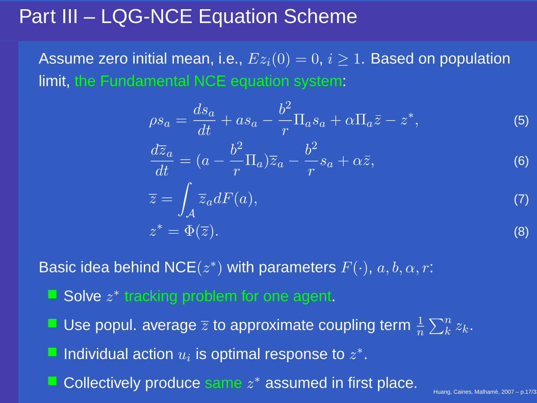
Part III – LQG-NCE Equation Scheme

Assume zero initial mean, i.e., Ezi(0) = 0, i ≥ 1. Based on population

limit, the Fundamental NCE equation system:

ρsa =dsa

dt+ asa −

b2

rΠasa + αΠaz − z∗, (5)

dza

dt= (a − b2

rΠa)za −

b2

rsa + αz, (6)

z =

∫

AzadF (a), (7)

z∗ = Φ(z). (8)

Basic idea behind NCE(z∗) with parameters F (·), a, b, α, r:

� Solve z∗ tracking problem for one agent.

� Use popul. average z to approximate coupling term 1n

∑nk zk.

� Individual action ui is optimal response to z∗.

� Collectively produce same z∗ assumed in first place.Huang, Caines, Malhame, 2007 – p.17/33

Part IV – Summary of NCE for LQG Model

Recall the system of n agents with dynamics:

dzi = aizidt + buidt + αz(n)dt + σidwi, 1 ≤ i ≤ n, t ≥ 0.

Let u−i denote (u1, · · · , un) with ui deleted, and express the indiv. cost

Ji(ui, u−i)△= E

∫ ∞

0e−ρt{[zi − Φ(

1

n

n∑

k=1

zk)]2 + ru2

i }dt.

Denote the optimal control for the tracking problem with si pre-computed

from the deterministic LQG NCE by

u0i = − b

r(Πizi + si), 1 ≤ i ≤ n,

revealing the closed-loop fixed point form of the large population tracking

problem!


Part IV – Main Existence Results

Theorem (Existence and Uniqueness ) The NCE(z∗) equation system has a

unique bounded solution (za, sa) for each a ∈ A subject to (H2)-(H3).

(H1) There exists a distribution F s.t. Fn → F weakly. (restated)

(H2) Φ is Lipschitz with parameter γ.

(H3) Gain condition:∫A[ |α|

β1(a) + b2(γ+|α|Πa)rβ1(a)β2(a) ]dF (a) < 1, and β1(a) > 0 for

all a ∈ A.

(H4) All agents have independent initial conditions with zero mean, and

supi≥1[σ2i + Ez2

i (0)] < ∞.


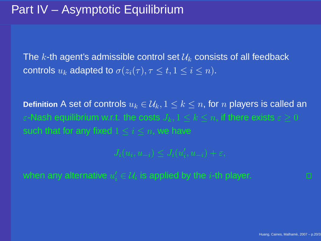
Part IV – Asymptotic Equilibrium

The k-th agent’s admissible control set Uk consists of all feedback

controls uk adapted to σ(zi(τ), τ ≤ t, 1 ≤ i ≤ n).

Definition A set of controls uk ∈ Uk, 1 ≤ k ≤ n, for n players is called an

ε-Nash equilibrium w.r.t. the costs Jk, 1 ≤ k ≤ n, if there exists ε ≥ 0

such that for any fixed 1 ≤ i ≤ n, we have

Ji(ui, u−i) ≤ Ji(u′i, u−i) + ε,

when any alternative u′i ∈ Ui is applied by the i-th player.


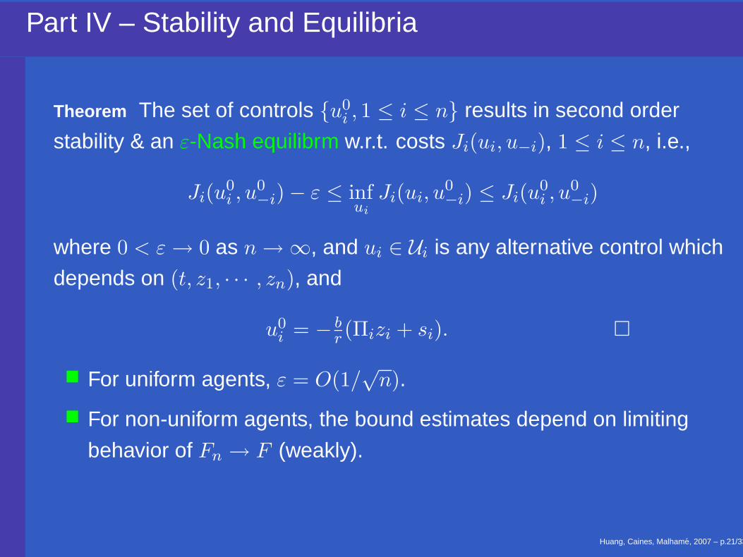
Part IV – Stability and Equilibria

Theorem The set of controls {u0i , 1 ≤ i ≤ n} results in second order

stability & an ε-Nash equilibrm w.r.t. costs Ji(ui, u−i), 1 ≤ i ≤ n, i.e.,

Ji(u0i , u

0−i) − ε ≤ inf

ui

Ji(ui, u0−i) ≤ Ji(u

0i , u

0−i)

where 0 < ε → 0 as n → ∞, and ui ∈ Ui is any alternative control which

depends on (t, z1, · · · , zn), and

u0i = − b

r(Πizi + si). �

� For uniform agents, ε = O(1/√

n).

� For non-uniform agents, the bound estimates depend on limiting

behavior of Fn → F (weakly).


Part IV – Implication for Rational Expectations

� Rational Expectations in Macroeconomic Theory. Issue of how

economic agents forecast future events (and hence play against

macroeconomic policy)

� NCE theory gives a coherent and tractable formulation of Rational

Expectations in game theoretic economic behavior with a large

number of players. In particular, NCE provides a means for

maintaining RE in that each individual can forecast

� the overall population behavior, and

� the associated optimal individual responses

� Implications for macroeconomic policy?


Part IV – Explicit Solutions for the NCE Equations

For a system of uniform agents with ai = a, Φ(z) = γ(z + η).

ρs =ds

dt+ as − b2

rΠs + αΠz − z∗,

NCE =⇒ dz

dt= (a − b2

rΠ)z + αz − b2

rs,

z∗ = φ(z) = γ(z + η).

⇓ (stead-state)

β2s(∞) − αΠz(∞) + z∗(∞) = 0

− b2

rs(∞) + (α − β1)z(∞) = 0

γz(∞) − z∗(∞) = −γη.

⇓unique solution


Part IV – Cost Gap

� Solve an LQG game model involving cost coupling with individual

cost Ji. Denote Nash equilibrium cost vind with population limit.

� Take welfare function J =∑n

i=1 Ji and compute optimal control with

cost vn. Optimal centralized control cost per agent v = limn→∞ vn/n.

� Cost gap: vind − v.

0 0.1 0.2 0.3 0.4 0.5 0.60

0.02

0.04

0.06

0.08

0.1

0.12

Horizontal axis −− Range of linking parameter γ in the cost

Indiv. cost by decentralized trackingLimit of centralized cost per agent: lim

n(v/n)

Cost Gap


Part V – Fully NL Models and McK-V-HJB Approach

� Dynamics:

dzi = (1/n)n∑

j=1

f(zi, ui, zj)dt + σdwi, 1 ≤ i ≤ n, t ≥ 0,

� Costs:

Ji(ui)△= E

∫ T

0

[(1/n)

n∑

j=1

L(zi, ui, zj)]dt, T < ∞.

� Control set: Each uk ∈ U compact.

� Other variants of the cost may be considered.

� Objective: look for decentralized strategies


Part V – Physics Counterpart: Particle Systems

� Interacting Particle Systems:

(IP) dxi =1

N

N∑

k=1

b(xi, xk)dt + σdwi, 1 ≤ i ≤ N,

with i.i.d. initial conditions.

� McKean-Vlasov equation:

(McK − V) dxt = b[xt, µt]dt + σdwt

where b[x, µt] =∫

b(x, y)µt(dy) for probability distribution µt.

� Definition The pair (xt, µt) is called a consistent pair if xt is a solution

to (McK-V) and µt is its distribution for all t ≥ 0.

� Intensively researched in: stochastic analysis (e.g. Dawson and

Gartner, 1987), physics, partial differential equations


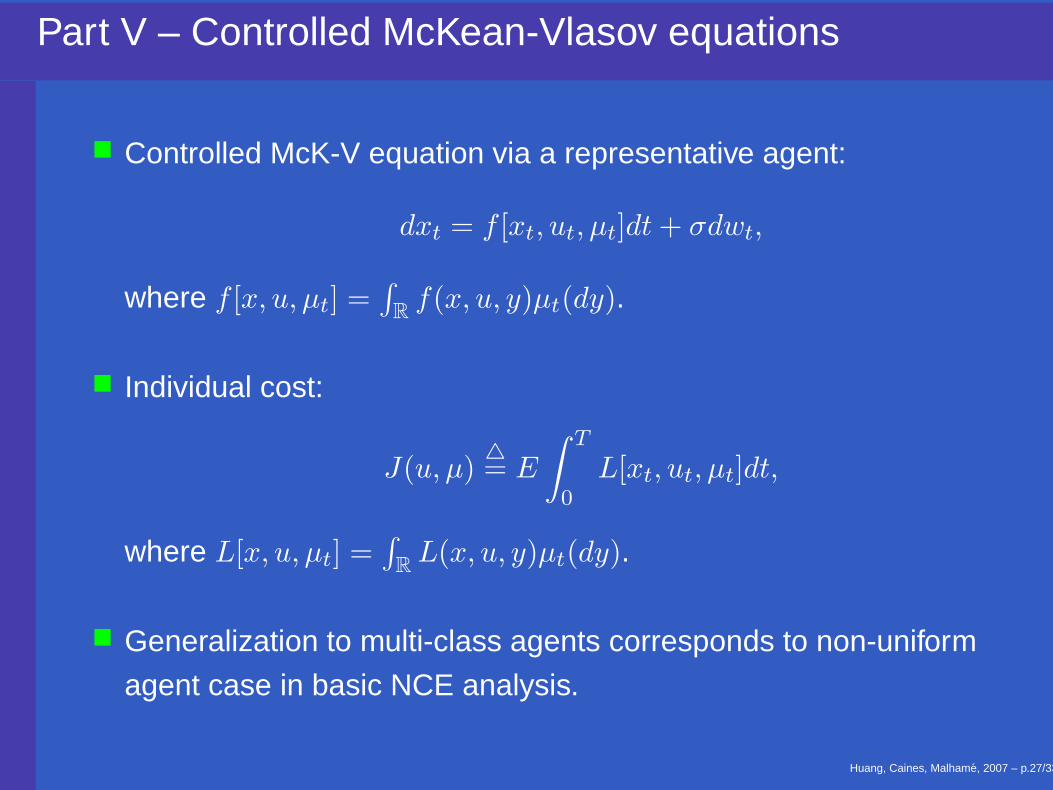
Part V – Controlled McKean-Vlasov equations

� Controlled McK-V equation via a representative agent:

dxt = f [xt, ut, µt]dt + σdwt,

where f [x, u, µt] =∫

Rf(x, u, y)µt(dy).

� Individual cost:

J(u, µ)△= E

∫ T

0L[xt, ut, µt]dt,

where L[x, u, µt] =∫

RL(x, u, y)µt(dy).

� Generalization to multi-class agents corresponds to non-uniform

agent case in basic NCE analysis.


Part V – The McK-V-NCE Principle

� Methodology: The key steps are to construct a mutually consistent

pair of

� (i) the mass effect, and

� (ii) the individual strategies such that the latter not only• (a) each constitute an optimal response to the mass effect• (b) but also collectively produce that mass effect.

� In non-uniform NCE-McKV setting, the mass effect is an average

w.r.t. the agent type distribution Fa.

� Principle: The application of an appropriate, general,

Fixed Point Theorem demonstrates that such a solution

� exists, is unique

� and is collectively produced by the actions of the individual

agents.


Part V – NCE and McK-V-HJB Theory

� HJB equation:

∂V

∂t= inf

u∈U

{f [x, u, µt]

∂V

∂x+ L[x, u, µt]

}+

σ2

2

∂2V

∂x2

V (T, x) = 0, (t, x) ∈ [0, T ) × R.

⇓

Optimal Control : ut = ϕ(t, x|µ·), (t, x) ∈ [0, T ] × R.

� Closed-loop McK-V equation:

dxt = f [xt, ϕ(t, x|µ·), µt]dt + σdwt, 0 ≤ t ≤ T.

The NCE methodology amounts to finding a solution (xt, µt) in McK-V

sense.


Part V –Outline of Analysis Based on NCE

By the NCE methodology, we carry out the steps:

� Construct controlled McKean-Vlasov equation; fixed point theory for

existence analysis

� Develop HJB equation (involving a measure flow) and derive Optimal

Response Mapping for individuals

� Establish existence results (for McK-V-HJB system)

� For equilibrium analysis – Approximate n “controlled interacting

particles" in closed-loop by n independent copies of the McK-V

equation


Part VI – Generalization to Multi-class Agents

� Dynamics:

dzi = (1/n)n∑

j=1

fai(zi, ui, zj)dt + σdwi, 1 ≤ i ≤ n, t ≥ 0,

where ai is the dynamic parameter, indicating type of agent.

� Costs:

Ji(ui)△= E

∫ T

0

[(1/n)

n∑

j=1

L(zi, ui, zj)]dt, T < ∞.

� Control set: Each uk ∈ U .

� The sequence {ai, i ≥ 1} takes value from A = {θ1, · · · , θK} with

empir. distri. (π1, · · · , πK), i.e., (1/n)∑n

i=1 1(ai=θk) → πk.


Part VI – Generalizat’n to Multi-class Agents (ctn)

� Controlled McK-V equation via a representative agent:

dxt = fa[xt, ut, µ1t , · · · , µK

t ]dt + σdwt,

where fa[x, u, µ1t , · · · , µK

t ] =∑K

k=1 πk

∫R

fa(x, u, y)µkt (dy).

� µkt reproduces the mass interaction generated by the class of agents

with parameter a = θk. (π1, · · · , πK): para empir. distri.

� Individual cost: J(u, µ)△= E

∫ T

0 L[xt, ut, µ1t , · · · , µK

t ]dt, where

L[x, u, µ1t , · · · , µK

t ] =∑K

k=1 πk

∫R

L(x, u, y)µt(dy).

� Distribution over agents would give generalized MKV HJB with

integral over the agents measures on the right hand side.


Concluding Remarks

� A theory for decentralized decision-making with many competing

agents

� Control synthesis via NCE methodology, and connection with

Rational Expectations in Macroeconomics

� Existence of asymptotic equilibrium (first in population limit)

� Application to dynamic pricing in network resource alloc. with hard

constraints (e.g. Pavel-Basar-Oldser)

� Closely related to physics of interacting particle systems

� This suggests the possibility of a convergence of control theory,

multi-agent systems and physics into a cybernetic – math physics

synthesis for competitive decision problems

� Related papers (03-07): http://www.math.carleton.ca/ mhuang/Huang, Caines, Malhame, 2007 – p.33/33

nash certainty equivalence in large population stochastic...

Documents