ZONA NASTRAN Data LoaderZNDAL

An Add-On to Tecplot® / Amtec Engineering, Inc.

User’s Manual

Copyright © –2001. All Rights Reserved.ZONA and ZNDAL are trademarks of ZONA Technology, Inc. Other product names are trademarks of their respective owners.

ZZZZZZZZOOOOOOOONNNNNNNNAAAAAAAA TTTTTTTTeeeeeeeecccccccchhhhhhhhnnnnnnnnoooooooollllllllooooooooggggggggyyyyyyyy,,,,,,,, IIIIIIIInnnnnnnncccccccc........7430 E. Stetson Drive, Ste. 205Scottsdale, AZ 85251-3540Tel (480) 945-9988/Fax (480) 945-6588info@zonatech.com / www.zonatech.com

1

ZONA NASTRAN Data Loader(A Graphical User Interface for NASTRAN’s Finite Element Analysis Software)

1.0 What is the ZONA NASTRAN Data Loader

The ZONA NASTRAN Data Loader (ZNDAL) is a Tecplot add-on developed by ZONATechnology, Inc. to allow for viewing of NASTRAN finite element models and basic outputanalysis results. As an input bulk data translator, ZNDAL can be used to view models to ensuremodeling accuracy before submitting a NASTRAN job or to copy three dimensional modelimages to other applications (e.g., Microsoft Word, PowerPoint, etc.). As a tool to view basicoutput analysis results, ZNDAL can be used to view structural displacements due to loads (staticanalysis), structural free vibration solutions (dynamic analysis), and stress contour plots (stressanalysis).

2.0 How Does ZNDAL Work

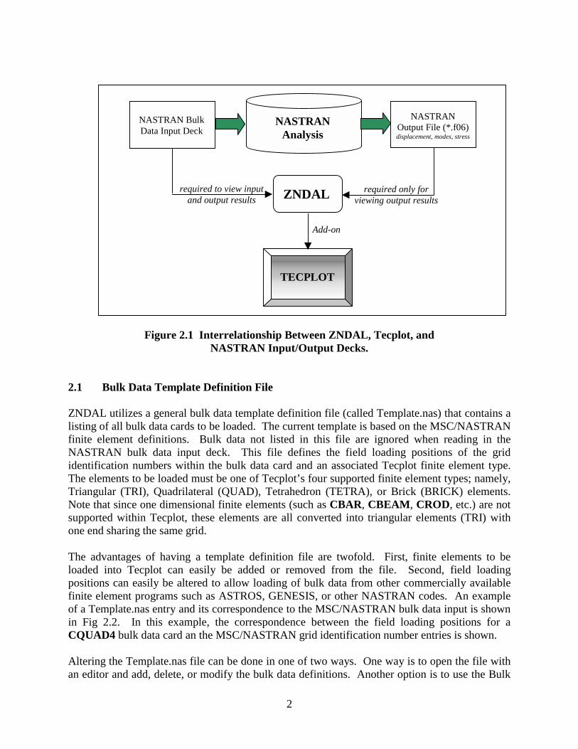
ZNDAL can read in and process a NASTRAN bulk data input deck for viewing the finiteelement model, as well as, read in and process the MSC/NASTRAN standard output file (i.e,*.f06 file) for viewing the static displacements, mode shapes, or grid point stress analysis results.ZNDAL utilizes a general bulk data definition template (described in section 2.1) that can easilybe modified to read bulk data input from most finite element analysis (FEA) software. Pleasenote: (1) the current bulk data definition template is specifically for MSC/NASTRAN inputfiles, and (2) the ZNDAL output processing is currently limited to the MSC/NASTRANstandard output format (i.e., the *.f06 output file). Figure 2.1 shows the interrelationshipbetween ZNDAL, Tecplot, and the NASTRAN input/output decks.

ZNDAL is designed to view the structural model and basic structural analysis output. It does notdisplay or process aerodynamic elements (such as those defined by CAERO1-CAERO5). Inaddition, only a NASTRAN structural analysis that leads to a structural displacement vector,eigenvalue/eigenvector, or stresses at grid points (as presented in section 4.0) in theMSC/NASTRAN output format can be loaded by ZNDAL.

Finally, viewing the finite element model alone only requires reading the NASTRAN bulk datainput deck. However, to display analysis results requires reading both the NASTRAN input andoutput decks into ZNDAL.

2

Figure 2.1 Interrelationship Between ZNDAL, Tecplot, andNASTRAN Input/Output Decks.

2.1 Bulk Data Template Definition File

ZNDAL utilizes a general bulk data template definition file (called Template.nas) that contains alisting of all bulk data cards to be loaded. The current template is based on the MSC/NASTRANfinite element definitions. Bulk data not listed in this file are ignored when reading in theNASTRAN bulk data input deck. This file defines the field loading positions of the grididentification numbers within the bulk data card and an associated Tecplot finite element type.The elements to be loaded must be one of Tecplot’s four supported finite element types; namely,Triangular (TRI), Quadrilateral (QUAD), Tetrahedron (TETRA), or Brick (BRICK) elements.Note that since one dimensional finite elements (such as CBAR, CBEAM, CROD, etc.) are notsupported within Tecplot, these elements are all converted into triangular elements (TRI) withone end sharing the same grid.

The advantages of having a template definition file are twofold. First, finite elements to beloaded into Tecplot can easily be added or removed from the file. Second, field loadingpositions can easily be altered to allow loading of bulk data from other commercially availablefinite element programs such as ASTROS, GENESIS, or other NASTRAN codes. An exampleof a Template.nas entry and its correspondence to the MSC/NASTRAN bulk data input is shownin Fig 2.2. In this example, the correspondence between the field loading positions for aCQUAD4 bulk data card an the MSC/NASTRAN grid identification number entries is shown.

Altering the Template.nas file can be done in one of two ways. One way is to open the file withan editor and add, delete, or modify the bulk data definitions. Another option is to use the Bulk

NASTRAN BulkData Input Deck

NASTRANAnalysis

NASTRANOutput File (*.f06)displacement, modes, stress

ZNDAL

TECPLOT

required to view inputand output results

required only forviewing output results

Add-on

3

Data Template button on the ZONA NASTRAN Data Loader window which will open theTemplate.nas file in Microsoft’s Notepad (see section 4.2, Item #3). The bulk data definitionscan then be altered and saved from Notepad. (It is recommended that you make a backup of theoriginal file before making changes.)

The bulk data template definition file must be input in the following fixed format:

Bulk DataTecplot Element

TypeNo. of Grids Blank Field Loading

Positions of GridsCharacter*8 Character*8 Integer*8 8x Integer*3

where

Bulk Data = name of bulk data to be loaded from NASTRAN input deckTecplot Element Type = one of the following element supported types: TRI = Triangle, QUAD = Quadrilateral, TETRA = Tetrahedron, BRICK = Brick.No. of GRIDS = number of GRID points that define the finite element (equal to the number of entries in the Field Loading Position. This value cannot be less than 2.)Blank = blank field 8 columns in widthField Loading Position = Fields in the bulk data input that reference GRID identification numbers

Note that 2-ended elements are loaded as triangular elements with 2 of the nodes sharing thesame location, 6-sided elements are condensed to triangular type elements (e.g., CTRIA6), and8-sided elements are condensed to quadrilateral elements (e.g., CQUAD8).

Comment cards (i.e., lines beginning with a $ in column 1) are allowed within the Template.nasfile as well as blank lines. Both are ignored by ZNDAL when reading this file.

$$* * * Template for NASTRAN bulk data input (fixed format) * * *$$ Tecplot$Bulk Element No. of$Data Type GRIDS Field Loading Positions of Grid ID's$(a8) (a8) (i8) blank (i3)$------|-------|-------| <-8x->|--|--|--|--|--|--|--|--|--|--|--|--|CBAR TRI 2 4 5CBEAM TRI 2 4 5CBEND TRI 2 4 5CBUSH TRI 2 4 5CBUSH1D TRI 2 4 5CELAS1 TRI 2 4 6CELAS2 TRI 2 4 6CHEXA BRICK 8 4 5 6 7 8 9 10 11CONROD TRI 2 3 4CQUAD4 QUAD 4 4 5 6 7

MSC/NASTRAN QuadrilateralPlate Element ConnectionFormat:

1 2 3 4 5 6 7 8 9 10

CQUAD4 EID PID G1 G2 G3 G4 THETA ZOFFS CONT

CONT T1 T2 T3 T4

4

Example:CQUAD4 111 202 30 74 75 32 2.6 0.3 +CQ1

+CQ1 1.77 2.01 3.02 1.80

Field ContentsEID Element identification number (Integer>0)PID Property identification number of a PSHELL, PCOMP, or PLPLANE entry

(Integer>0; Default=EID)Gi Grid point identification number of connection points (Integer > 0, all unique)THETA Material property orientation angle in degrees.MCID Material coordinate system identification number. (Integer≥0; If blank, then

THETA=0.0)ZOFFS Offset from the surface of grid points to the element reference plane (Real)Ti Membrane thickness of element at grid points G1 through G4. (Real≥0.0)

Figure 2.2 Example of the Relationship Between Template.nas Field LoadingPositions and MSC/NASTRAN Bulk Data Input.

2.2 Bulk Data Input File Processing Procedure

Since bulk data can be input in an arbitrary fashion and/or in free format, ZNDAL first generatesa new file with a filename extension of *.fix_01z that contains a formatted version of the originalbulk data deck beginning from the BEGIN BULK statement and ending at the ENDDATAstatement. All comments (i.e., rows with a $ in column 1) are removed from this file and alllower case characters are converted to upper case. Free formatted input (i.e., field data separatedby commas) are also converted to fixed format within this file.

ZNDAL then reads the *.fix_01z file to read in all of the coordinate system definitions declaredin the bulk data input. The MSC/NASTRAN coordinate system definition cards supported are:

CORD1C cylindrical coordinate system using three grid pointsCORD1R rectangular coordinate system using three grid pointsCORD1S spherical coordinate system using three grid pointsCORD2C cylindrical coordinate system using three pointsCORD1R rectangular coordinate system using three pointsCORD1S spherical coordinate system using three points

Coordinate systems that reference other coordinate systems are allowed and accounted for inZNDAL. With all coordinate systems read in, ZNDAL generates transformation matricesrequired to convert all grid points defined in local coordinate systems back into the basic system.A new file with a filename extension of *.cor_01z is then generated with a new bulk data deckthat contains the entire model in the basic system.

5

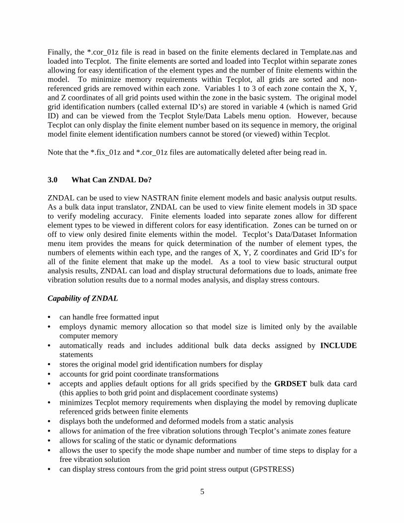
Finally, the *.cor_01z file is read in based on the finite elements declared in Template.nas andloaded into Tecplot. The finite elements are sorted and loaded into Tecplot within separate zonesallowing for easy identification of the element types and the number of finite elements within themodel. To minimize memory requirements within Tecplot, all grids are sorted and non-referenced grids are removed within each zone. Variables 1 to 3 of each zone contain the X, Y,and Z coordinates of all grid points used within the zone in the basic system. The original modelgrid identification numbers (called external ID’s) are stored in variable 4 (which is named GridID) and can be viewed from the Tecplot Style/Data Labels menu option. However, becauseTecplot can only display the finite element number based on its sequence in memory, the originalmodel finite element identification numbers cannot be stored (or viewed) within Tecplot.

Note that the *.fix_01z and *.cor_01z files are automatically deleted after being read in.

3.0 What Can ZNDAL Do?

ZNDAL can be used to view NASTRAN finite element models and basic analysis output results.As a bulk data input translator, ZNDAL can be used to view finite element models in 3D spaceto verify modeling accuracy. Finite elements loaded into separate zones allow for differentelement types to be viewed in different colors for easy identification. Zones can be turned on oroff to view only desired finite elements within the model. Tecplot’s Data/Dataset Informationmenu item provides the means for quick determination of the number of element types, thenumbers of elements within each type, and the ranges of X, Y, Z coordinates and Grid ID’s forall of the finite element that make up the model. As a tool to view basic structural outputanalysis results, ZNDAL can load and display structural deformations due to loads, animate freevibration solution results due to a normal modes analysis, and display stress contours.

Capability of ZNDAL

• can handle free formatted input• employs dynamic memory allocation so that model size is limited only by the available

computer memory• automatically reads and includes additional bulk data decks assigned by INCLUDE

statements• stores the original model grid identification numbers for display• accounts for grid point coordinate transformations• accepts and applies default options for all grids specified by the GRDSET bulk data card

(this applies to both grid point and displacement coordinate systems)• minimizes Tecplot memory requirements when displaying the model by removing duplicate

referenced grids between finite elements• displays both the undeformed and deformed models from a static analysis• allows for animation of the free vibration solutions through Tecplot’s animate zones feature• allows for scaling of the static or dynamic deformations• allows the user to specify the mode shape number and number of time steps to display for a

free vibration solution• can display stress contours from the grid point stress output (GPSTRESS)

6

• accounts for displacement coordinate system transformations• displays mode number and natural frequency in the frame title• locates and reads finite element model title and assigns the it to the frame title (defaults to

“NASTRAN Bulk Data File: filename”)

Limitations of ZNDAL

• cannot perform grid replication (this can be done by NASTRAN with ECHO=PUNCH)• cannot read large field input due to multiple lines (except for GRID* and CORDxx* which

are supported)• cannot display finite element identification numbers due to Tecplot supported data format• cannot load or display scalar points (e.g., CELAS1 with G1 or G2 left blank)• does not process separated continuation lines allowable within NASTRAN’s unique

continuation card requirement. However, this only becomes an issue for bulk data cards withthat require two or more lines of input to define all of the grids (e.g., CQUAD8).

• cannot display stresses on 1-dimensional elements• does not process aerodynamic macroelements such as CAERO1-CAERO5 bulk data cards• although possible, it is not recommended to load models with more than 100,000 elements

since sorting is done in-core (loading can take several minutes for large models).

7

4.0 Using ZNDAL

The following sections will describe how to load and view the finite element model and outputanalysis results using a simple cantilever plate structure example.

4.1 Description of the Problem

A static and dynamic analysis of a simple cantilever plate structure is considered (see Fig 4.1).The structure consists of an aluminum plate with a thickness of t=0.25 inches. The modulus ofelasticity, Poisson’s ratio, and mass density are E=1.07E+07 psi, ν=0.33, and ρ=2.59E-04slinch/in3 (=0.1 lb/in3), respectively. The plate is fully clamped at one end and two forces of 400lb are applied to the free end as shown.

Figure 4.1 Simple Cantilever Plate with Applied Forces.

To generate a corresponding finite element model, the structure is discretized by plate elements(CQUAD4) as shown in Fig 4.2. Grid points are sequenced from the clamped end towards thefree end as shown. The bulk data deck for this case is shown in Table 4.1.

To perform a static analysis, a solution sequence of 101 is selected (SOL 101). Both thestructural displacement due to the applied loads and the grid point stresses are requested in theCase Control section. A LOAD=300 is specified to refer to the LOAD bulk data card. Note thatDISP=ALL, STRESS=ALL, and GPSTRESS=ALL should be selected to obtain grid pointdisplacements and stresses for all grids within the model. A SURFACE and/or VOLUMEcommand must be properly specified in the OUTPUT(POST) section of the Case Control sectionin order for the output request for grid point stresses to be properly generated. The user is

L = 6 in

W = 3 in

F = 400 lb

F = 400 lb

t = 0.25 in

8

encouraged to review the MSC/NASTRAN Quick Reference and Linear Static Analysis guidesfor a detailed description of this process.

1

2

5 3

46

9 7

8

13

10

14

11

12

15

16

Figure 4.2 Finite Element Model of the Simple Cantilever Plate Structure.

Table 4.1 Bulk Data Input Deck of the Simple Cantilever Plate (file: plate-s.dat).

$ CANTILEVER PLATE TEST CASE FOR ZNDALID MSC, PLATESOL 101CENDTITLE= DEMONSTRATION PROBLEM, CANTILEVERED PLATESUBTITLE= STATIC ANALYSISSUBCASE 10LABEL= TIP APPLIED NORMAL FORCEFORCE=ALLSTRESS=ALLSTRAIN=ALLLOAD=300SPC=102OLOAD=ALLSPCFORCES=ALLDISP=ALLGPFORCE=ALLESE=ALLGPSTRESS=ALLOUTPUT(POST)SET 100 = ALLSURFACE 5 SET 100$BEGIN BULKPARAM AUTOSPC YESPARAM GRDPNT 0$---1--|---2---|---3---|---4---|---5---|---6---|---7---|---8---|---9---|--10---|GRID 1 0.0 0.0 0.0GRID 2 0.0 1.0 0.0GRID 3 0.0 2.0 0.0GRID 4 0.0 3.0 0.0GRID 5 2.0 0.0 0.0GRID 6 2.0 1.0 0.0GRID 7 2.0 2.0 0.0GRID 8 2.0 3.0 0.0

9

GRID 9 4.0 0.0 0.0GRID 10 4.0 1.0 0.0GRID 11 4.0 2.0 0.0GRID 12 4.0 3.0 0.0GRID 13 6.0 0.0 0.0GRID 14 6.0 1.0 0.0GRID 15 6.0 2.0 0.0GRID 16 6.0 3.0 0.0CQUAD4 11 21 1 5 6 2CQUAD4 12 21 2 6 7 3CQUAD4 13 21 3 7 8 4CQUAD4 14 21 5 9 10 6CQUAD4 15 21 6 10 11 7CQUAD4 16 21 7 11 12 8CQUAD4 17 21 9 13 14 10CQUAD4 18 21 10 14 15 11CQUAD4 19 21 11 15 16 12$ STATIC LOAD (APPLIED FORCES)$---1--|---2---|---3---|---4---|---5---|---6---|---7---|---8---|---9---|--10---|LOAD 300 1. 1. 100 1. 200FORCE 100 16 400. -1.0FORCE 200 13 400. 1.0$MAT1 31 1.07+07 .33 2.59-04 +MAT1+MAT1 60000. 60000. 40000.PLOAD2 100 1. 11 THRU 14PSHELL 21 31 .25 31SPC1 102 123456 1 2 3 4ENDDATA

To perform a dynamic analysis for obtaining the free vibration solutions of the structure, theCase Control section is altered as shown in Table 4.2. A solution sequence of 103 is selected(SOL 103). A METHOD=10 command is specified to refer to a real eigenvalue extraction bulkdata card (EIGR). Ten modes are specified as the desired number of roots. As with the staticanalysis case, DISP=ALL must be specified in order to generate the modal displacements at allgrid points.

Table 4.2 Bulk Data Input Deck of the Simple Cantilever Plate (file: plate-d.dat).

$ CANTILEVER PLATE TEST CASE FOR ZNDALID MSC, PLATESOL 103CENDTITLE= DEMONSTRATION PROBLEM, CANTILEVERED PLATESUBTITLE= DYNAMIC ANALYSISSUBCASE 10LABEL= FREE VIBRATION SOLUTIONMETHOD=10SPC=102DISP=ALL$BEGIN BULKPARAM AUTOSPC YESPARAM GRDPNT 0EIGR 10 MGIV 0.0 500. 10 +ER+ER MAX$---1--|---2---|---3---|---4---|---5---|---6---|---7---|---8---|---9---|--10---|GRID 1 0.0 0.0 0.0GRID 2 0.0 1.0 0.0

.

.

.

10

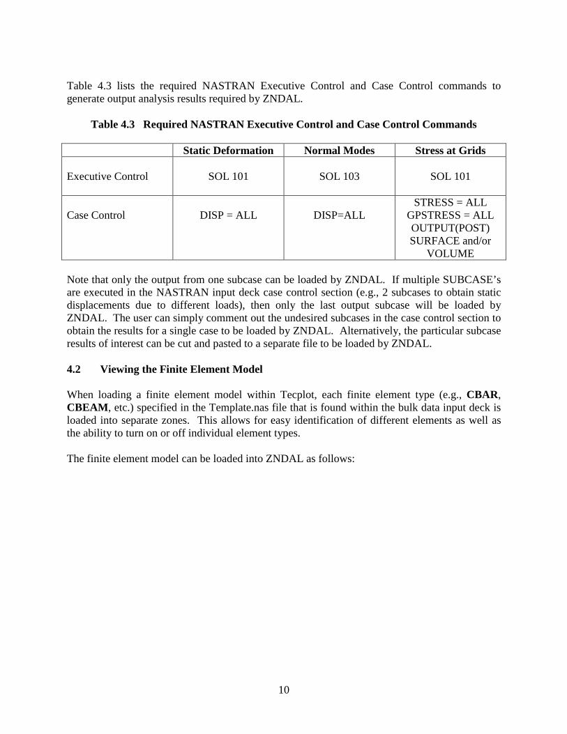
Table 4.3 lists the required NASTRAN Executive Control and Case Control commands togenerate output analysis results required by ZNDAL.

Table 4.3 Required NASTRAN Executive Control and Case Control Commands

Static Deformation Normal Modes Stress at Grids

Executive Control SOL 101 SOL 103 SOL 101

Case Control DISP = ALL DISP=ALLSTRESS = ALL

GPSTRESS = ALLOUTPUT(POST)SURFACE and/or

VOLUME

Note that only the output from one subcase can be loaded by ZNDAL. If multiple SUBCASE’sare executed in the NASTRAN input deck case control section (e.g., 2 subcases to obtain staticdisplacements due to different loads), then only the last output subcase will be loaded byZNDAL. The user can simply comment out the undesired subcases in the case control section toobtain the results for a single case to be loaded by ZNDAL. Alternatively, the particular subcaseresults of interest can be cut and pasted to a separate file to be loaded by ZNDAL.

4.2 Viewing the Finite Element Model

When loading a finite element model within Tecplot, each finite element type (e.g., CBAR,CBEAM, etc.) specified in the Template.nas file that is found within the bulk data input deck isloaded into separate zones. This allows for easy identification of different elements as well asthe ability to turn on or off individual element types.

The finite element model can be loaded into ZNDAL as follows:

11

1. From the Tecplot File menu select Import

2. From the Select Import Format window choose the “ZONA NASTRAN Data Loader” optionand click on OK.

3. From the ZONA NASTRAN Data Loader window, click on the NASTRAN Bulk Data InputDeck Only button to select the bulk data deck to be loaded (in this case: plate-s.dat). Afterselecting the file, click on OK.

12

4. A status bar will show the file translation progress. For extremely large Input/Output decks,this process can take several minutes while the program loads and translates all of the data.

5. If no errors are encountered, the NASTRAN model will be displayed in Tecplot in a 3D viewwith the X-Y-Z axis dependency set to 1-1-1.

13

Some Useful Capabilities:

- To view information about the finite elements within the model, select DataSet Info from theData menu. From this window, the number of finite elements and grid points used by eachzone can be determined, as well as, the range of values for the X, Y, Z coordinates and grididentification numbers within each zone.

- To turn on/off grid point identification numbers, select Data Labels from the Style menu andclick on the Show Node Labels and select Grid ID from the Show Variable Value drop downmenu.

- The Tecplot tools on the toolbar can be used to orient and zoom-in/out of the model. ThePlot Attributes button (Mesh tab) can be used to identify finite elements by color as well asturn on or off individual finite elements.

- Grid point information (e.g., coordinates, Grid Id and stresses if viewing stress results) can beobtained by choosing the icon from the toolbar, holding the CNTL key, and clicking onthe desired grid point.

14

4.3 Viewing the NASTRAN Analysis Results

In order to view the NASTRAN analysis results requires reading in both the finite element modelinput deck as well as analysis output file (i.e., *.f06 file). The specific analysis output desired(displacement, modes, or stress) must exist in the NASTRAN standard output file in order forZNDAL to be able to display the results.

The NASTRAN analysis output can be loaded by ZNDAL as follows:

1. Follow steps #1 and #2 from section 4.2.

2. From the ZONA NASTRAN Data Loader window, click on the NASTRAN Bulk Data InputDeck and Output File button to select the input and output files to be loaded.

3. Select the output analysis type. For the Static Deformation, only an Amplification Factor canbe specified. For the Normal Modes, the Amplification Factor, No. of Time Steps, and Mode

15

Number can be specified. For Stress, none of these are required. The default values forAmplification Factor is 100%, for No. of Time Steps is 1, and for Mode No. is 1. Adescription of each of these will be provided in the following sections.

4. Click on OK and the finite element model and analysis results will be loaded.

4.3.1 Static Deformation due to Applied Load(s)

Input / Output Cases = plate-s.dat / plate-s.f06

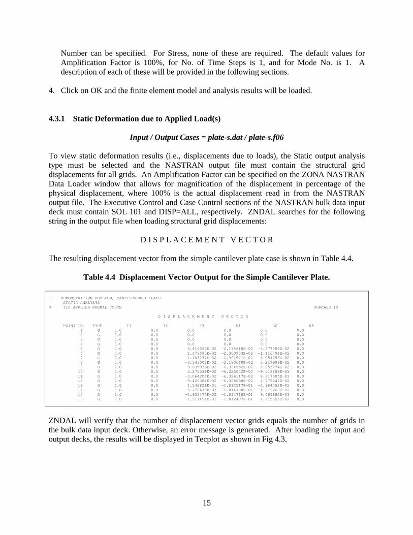
To view static deformation results (i.e., displacements due to loads), the Static output analysistype must be selected and the NASTRAN output file must contain the structural griddisplacements for all grids. An Amplification Factor can be specified on the ZONA NASTRANData Loader window that allows for magnification of the displacement in percentage of thephysical displacement, where 100% is the actual displacement read in from the NASTRANoutput file. The Executive Control and Case Control sections of the NASTRAN bulk data inputdeck must contain SOL 101 and DISP=ALL, respectively. ZNDAL searches for the followingstring in the output file when loading structural grid displacements:

D I S P L A C E M E N T V E C T O R

The resulting displacement vector from the simple cantilever plate case is shown in Table 4.4.

Table 4.4 Displacement Vector Output for the Simple Cantilever Plate.

1 DEMONSTRATION PROBLEM, CANTILEVERED PLATESTATIC ANALYSIS

0 TIP APPLIED NORMAL FORCE SUBCASE 10

D I S P L A C E M E N T V E C T O R

POINT ID. TYPE T1 T2 T3 R1 R2 R31 G 0.0 0.0 0.0 0.0 0.0 0.02 G 0.0 0.0 0.0 0.0 0.0 0.03 G 0.0 0.0 0.0 0.0 0.0 0.04 G 0.0 0.0 0.0 0.0 0.0 0.05 G 0.0 0.0 3.416093E-02 -2.174618E-02 -3.277006E-02 0.06 G 0.0 0.0 1.179590E-02 -2.300903E-02 -1.116794E-02 0.07 G 0.0 0.0 -1.103277E-02 -2.301571E-02 1.054758E-02 0.08 G 0.0 0.0 -3.343002E-02 -2.180668E-02 3.217999E-02 0.09 G 0.0 0.0 9.635836E-02 -6.364952E-02 -2.853874E-02 0.010 G 0.0 0.0 3.275036E-02 -6.325042E-02 -9.513888E-03 0.011 G 0.0 0.0 -3.064204E-02 -6.326117E-02 8.817085E-03 0.012 G 0.0 0.0 -9.426384E-02 -6.366668E-02 2.779446E-02 0.013 G 0.0 0.0 1.546821E-01 -1.012517E-01 -2.884752E-02 0.014 G 0.0 0.0 5.276679E-02 -1.014700E-01 -1.019263E-02 0.015 G 0.0 0.0 -4.923470E-02 -1.014710E-01 9.465682E-03 0.016 G 0.0 0.0 -1.511494E-01 -1.012497E-01 2.815355E-02 0.0

ZNDAL will verify that the number of displacement vector grids equals the number of grids inthe bulk data input deck. Otherwise, an error message is generated. After loading the input andoutput decks, the results will be displayed in Tecplot as shown in Fig 4.3.

16

Figure 4.3 Static Deformation of the Simple Cantilever Plate due to Tip Loads.

Both the undeformed (in red) and deformed (in green) models are displayed. The number ofzones loaded within Tecplot for a static analysis results case is equal to two times the number offinite element types read in from the bulk data input deck. For example, if the bulk data inputdeck has CBAR, CELAS2, CTRIA3, and CQUAD4 elements, then the number of zones loadedinto Tecplot would be 2 x 4 = 8. For each finite element type loaded, first the undeformedelements are loaded followed by the deformed counterpart. The deformed elements are namedwithin Tecplot with the extension –STATIC DISP. All element zone names can be viewed fromthe Data/DataSet Info menu item on the Zone/Variable Info tab.

4.3.2 Viewing the Free Vibration Solutions

Input / Output Cases = plate-d.dat / plate-d.f06

A powerful feature within ZNDAL is the ability to load the finite element model free vibrationsolution results and alter the finite element model in such a way as to allow for animation of themode shapes. This is in contrast to only viewing a static deformation of a given mode shape.

To view the free vibration solutions results, the Normal Modes analysis type must be selectedand the NASTRAN output file must contain the eigenvalue and eigenvector solutions. As withthe static deformation case, an Amplification Factor can be specified on the ZONA NASTRANData Loader window that allows for scaling of the displacement in percentage of the physicaldisplacement, where 100% is the actual displacement read in from the NASTRAN output file.The No. of Time Steps can be input which specifies the desired number of zones to be generatedwithin Tecplot (default=1), and the Mode No. is the mode shape eigenvector to be read in anddisplayed (default=mode 1). The Mode No. requested must, of course, exist in the NASTRANoutput file. The Executive Control and Case Control sections of the NASTRAN bulk data inputdeck must contain SOL 103 and DISP=ALL, respectively. ZNDAL searches for the followingstring in the output file when loading the free vibration solutions:

17

R E A L E I G E N V A L U E S

followed by the keyword CYCLES when searching for the requested eigenvector (i.e., Mode No.specified in the ZONA NASTRAN Data Loader window).

A sample of the resulting eigenvalue/eigenvector from the simple cantilever plate case is shownin Table 4.5.

Table 4.5 Eigenvalue/Eigenvector Output of the Simple Cantilever Plate.

1 DEMONSTRATION PROBLEM, CANTILEVERED PLATEDYNAMIC ANALYSIS

0 SUBCASE 10

R E A L E I G E N V A L U E SMODE EXTRACTION EIGENVALUE RADIANS CYCLES GENERALIZED GENERALIZEDNO. ORDER MASS STIFFNESS

1 25 1.990045E+06 1.410689E+03 2.245182E+02 3.141556E-04 6.251838E+022 26 3.133214E+07 5.597512E+03 8.908716E+02 1.911755E-04 5.989938E+033 27 6.315864E+07 7.947241E+03 1.264843E+03 5.607960E-04 3.541911E+044 1 2.123881E+08 1.457354E+04 2.319451E+03 3.630742E-04 7.711262E+045 28 2.818252E+08 1.678765E+04 2.671838E+03 1.527733E-04 4.305537E+04

.

.

.

1 DEMONSTRATION PROBLEM, CANTILEVERED PLATEDYNAMIC ANALYSIS

0 FREE VIBRATION SOLUTION SUBCASE 10EIGENVALUE = 1.990045E+06

CYCLES = 2.245182E+02 R E A L E I G E N V E C T O R N O . 1

POINT ID. TYPE T1 T2 T3 R1 R2 R31 G 0.0 0.0 0.0 0.0 0.0 0.02 G 0.0 0.0 0.0 0.0 0.0 0.03 G 0.0 0.0 0.0 0.0 0.0 0.04 G 0.0 0.0 0.0 0.0 0.0 0.05 G 0.0 0.0 1.500228E-01 2.076070E-02 -1.373344E-01 0.06 G 0.0 0.0 1.619293E-01 3.675800E-03 -1.486413E-01 0.07 G 0.0 0.0 1.619293E-01 -3.675800E-03 -1.486413E-01 0.08 G 0.0 0.0 1.500228E-01 -2.076070E-02 -1.373344E-01 0.0

.

.

.

In order to view the free vibration solution within Tecplot’s animated zones feature, the entirefinite element model is broken down into one dimensional elements to be loaded within a singlezone. Additional zones are used to load the deformed model at different time steps within onecycle of oscillation. The number of zones created is equal to one plus the No. of Time Steps thatis specified on the ZONA NASTRAN Data Loader window (the first zone being at time t=0 sec).The physical (true) time at each step is computed from the natural frequency of the mode (whichis read in from the NASTRAN output file) and the No. of Time Steps as follows:

�=

���

����

�

⋅ωπ⋅=

NTIME

0i ni NTIME

2it

18

where

i = index of the time stepti = the time of the i’th deformed NASTRAN modelωn = natural frequency in HzNTIME = No. of Time Steps specified in the ZONA NASTRAN Data Loader window

The displacment vector v� for each grid is then computed from

( )in0 tsinvv ⋅ω⋅= ��

where

0v� = the grid eigenvector of the Mode No. specified in the NASTRAN Bulk Data Loader window

The new displacement vector v� computed for each grid in the structural model is then applied tothe corresponding grid in the undeformed model.

ZNDAL will verify that the number of real eigenvector grids equals the number of grids in thebulk data input deck. Otherwise, an error message is generated. After loading the input andoutput decks, the results will be displayed in Tecplot as shown in Fig 4.4.

X Y

ZFrame 001 21 Jun 2001 DEMONSTRATION PROBLEM, CANTILEVERED PLAT |Mode No.= 1|Frequency= 2.24518E+02 HzFrame 001 21 Jun 2001 DEMONSTRATION PROBLEM, CANTILEVERED PLAT |Mode No.= 1|Frequency= 2.24518E+02 Hz

Figure 4.4 Free Vibration Solution of the Simple Cantilever Plate (Mode 1, 224.5 Hz).

19

The mode shape can be animated by using the Tools/Animate Zones feature and displaying eachzone successively (the Animate button can be used for this purpose). Also output to Tecplot arethe physical times (in seconds) for each position of the displacement which are saved as the titlesof each zone. Finally, the NASTRAN input deck title, mode number, and natural frequency areoutput on the Tecplot frame for convenience.

4.3.3 Viewing the Stress Distribution

Input / Output Cases = plate-s.dat / plate-s.f06

Viewing the stress distributions within the structural model requires that the NASTRAN gridpoint stress generator (GPSTRESS) be employed. The GPSTRESS methodinterpolates/extrapolates a set of element stresses over a surface or volume to obtain average gridpoint stresses. A SURFACE and/or VOLUME Case Control command must be defined in theOUTPUT(POST) section for this method to work. The user is responsible for defining theproper coordinate system for stress output within this method. Details in the GPSTRESS methodare complicated and outside the scope of this document. The user is referred to theMSC/NASTRAN Linear Static Analysis guide for a detailed description.

To view stress distribution results, the Stress at Grids output analysis type must be selected andthe NASTRAN output file must contain the grid point stresses. The Executive Control sectionshould contain SOL 101 while the Case Control section must specify, STRESS=ALL,GPSTRESS=ALL, OUTPUT(POST), and must define a SURFACE and/or VOLUME entry.

Note that stresses due to normal modes or transient analyses can also be loaded, but the usermust first remove all grid point stress results from the NASTRAN output file that are not to beviewed. Otherwise and error results indicating that more grid point stress values exist that gridsin the bulk data input deck. Grid points within the model that do not have resulting stress valuesin the output file are all set to zero. ZNDAL searches for the following string in the output filewhen loading grid point stresses:

S T R E S S E S A T G R I D P O I N T S(for SURFACE grids)

and

D I R E C T S T R E S S E S A T G R I D P O I N T S(for VOLUME grids)

A sample of the resulting grid point stresses for SURFACE grids from the simple cantilever platecase is shown in Table 4.6.

20

Table 4.6 Grid Point Stress Output of the Simple Cantilever Plate.

1 DEMONSTRATION PROBLEM, CANTILEVERED PLATESTATIC ANALYSIS

0 TIP APPLIED NORMAL FORCE SUBCASE 10SUBCASE = 10

S T R E S S E S A T G R I D P O I N T S - - S U R F A C E 50 SURFACE X-AXIS X NORMAL(Z-AXIS) R REFERENCE COORDINATE SYSTEM FOR SURFACE DEFINITION CID0

GRID ELEMENT STRESSES IN SURFACE SYSTEM PRINCIPAL STRESSES MAXID ID FIBER NORMAL-X NORMAL-Y SHEAR-XY ANGLE MAJOR MINOR SHEAR VON MISES

0 1 0 Z1 2.885E+04 8.190E+03 -6.357E+03 -15.8057 3.065E+04 6.391E+03 1.213E+04 2.800E+04Z2 -2.885E+04 -8.190E+03 6.357E+03 74.1943 -6.391E+03 -3.065E+04 1.213E+04 2.800E+04

MID 0.000E+00 0.000E+00 0.000E+00 0.0 0.000E+00 0.000E+00 0.000E+00 0.000E+000 2 0 Z1 1.290E+04 3.769E+03 -6.545E+03 -27.5454 1.632E+04 3.551E+02 7.981E+03 1.614E+04

Z2 -1.290E+04 -3.769E+03 6.545E+03 62.4546 -3.551E+02 -1.632E+04 7.981E+03 1.614E+04MID 0.000E+00 0.000E+00 0.000E+00 0.0 0.000E+00 0.000E+00 0.000E+00 0.000E+00

Between the SURFACE and VOLUME grid point stress output, 29 different stress componentscan be output to the NASTRAN output file. All 29 components are loaded into Tecplot and caneach be viewed independently. These 29 stress components are:

For SURFACE grid point stressesUpperSurface (Z1) Normal-X Normal-Y Shear XY Major Minor Max Shear von MisesLowerSurface (Z2) Normal-X Normal-Y Shear XY Major Minor Max Shear von MisesMid-Plane(MID) Normal-X Normal-Y Shear XY Major Minor Max Shear von Mises

For VOLUME grid point stresses

Normal-X Normal-Y Normal-Z Shear XY Shear YZ

A picture of the volume element stresses would be similar tin the Z-direction as well.

ZNDAL will verify that the number of grids with stress valuof grids in the bulk data input deck. Otherwise, an error meinput and output decks, the results will be displayed in Tecorder to view the contour plot, the contour option must baddition, from the Plot Attributes button/Contour tab, theFlood.

Zelem Yelem

σx

σx

Xelem

σy

σy

τxy

τxy

Shear ZX Mean Pres von Mises

o above except that the stresses exist

es is less than or equal to the numberssage is generated. After loading theplot as shown in Fig 4.5. Note: In

e selected from within Tecplot. In Contour Plottype should be set to

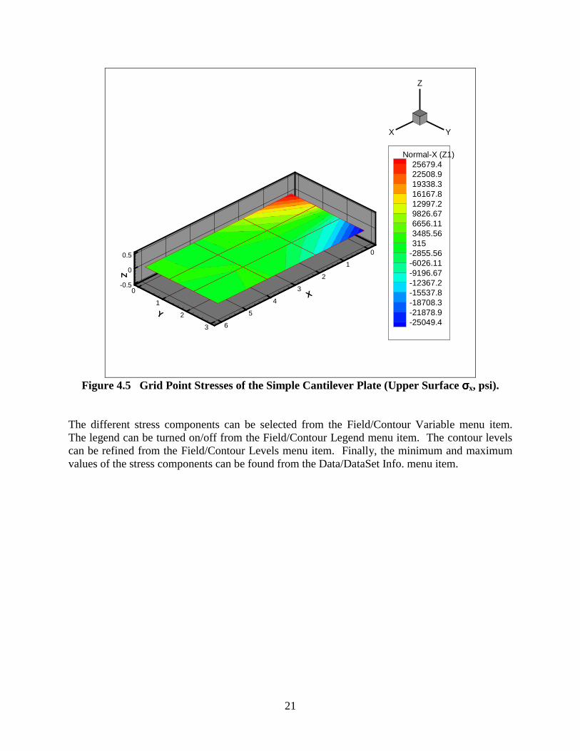
21

-0.5

0

0.5

Z

0

1

2

3

4

5

6

X0

1

2

3

Y

X Y

Z

Normal-X (Z1)25679.422508.919338.316167.812997.29826.676656.113485.56315

-2855.56-6026.11-9196.67-12367.2-15537.8-18708.3-21878.9-25049.4

Figure 4.5 Grid Point Stresses of the Simple Cantilever Plate (Upper Surface σσσσx, psi).

The different stress components can be selected from the Field/Contour Variable menu item.The legend can be turned on/off from the Field/Contour Legend menu item. The contour levelscan be refined from the Field/Contour Levels menu item. Finally, the minimum and maximumvalues of the stress components can be found from the Data/DataSet Info. menu item.