national college of ireland
TRANSCRIPT

National College of Ireland BSHTM – Technology Management
Data Analytic
Year 4 2020/2021
Punnavit Kaewhin
X17713929
Trends and Patterns within life expectancy data.
Technical Report

1
Contents Executive Summary ................................................................................................................................. 2
1.0 Introduction ................................................................................................................................ 3
1.1. Background ............................................................................................................................. 3
1.2. Aims ......................................................................................................................................... 4
1.3. Technology .............................................................................................................................. 4
1.4. Structure ................................................................................................................................. 4
2.0 Data ............................................................................................................................................. 5
3.0 Methodology ............................................................................................................................... 6
4.0 Analysis ....................................................................................................................................... 7
5.0 Results ......................................................................................................................................... 9
6.0 Conclusions ............................................................................................................................... 24
7.0 Further Development or Research ........................................................................................... 25
8.0 References ................................................................................................................................ 26
9.0 Appendices ................................................................................................................................ 27
9.1. Project Plan ........................................................................................................................... 27
9.2. Ethics Approval Application (only if required) ...................................................................... 27
9.3. Reflective Journals ................................................................................................................ 27
9.4. Proposal ................................................................................... Error! Bookmark not defined.
2
Executive Summary This project purposes is to study the dataset provided by the World Health Organisation on the life expectancy of Countries around the world. With hope of learning something interesting from the said dataset and implement a datamining technique on it for prediction. The dataset would be studied using the program SPSS and R studio to analyse for specific result.
The dataset will be studied under the datamining technique of KDD or Knowledge Discovery in Databases. Which will include processes such as selection, pre-processing, transforming, datamining, and interpretation/evaluation. But first of a set of general testing was carried out in SPSS, test for things such as normality before going ahead with the actual prediction. The main scope of this project was to find out an appropriate method to be able to forecast a satisfying result. The results achieve should be interpreted carefully and with reservation, as due to the nature of the data there is not enough sufficient data for an “accurate” forecasting.
Overall Summary of the normality test as expected, was that the data was not normally distributed. This is due to the nature of the data set and how it was collected and sorted. This is because the data was collected overtime by WHO and then analyse and sort by them first before being put out by the public, hence the average life expectancy figure for each year. Thus, the data cannot be random and normally distributed, ensuring that a non-parametric test is needed.
Lastly it needs to be stated again that the key method used is for forecasting is called Arima modelling, and it usually works better when there is more sufficient data to work with (more than 30). But in this case, there is only about 14/15 per country. Hence the warning about the result mentioned earlier.

3
1.0 Introduction 1.1. Background I took this project idea because I like the idea of how living condition improve each year
due to new invention, discoveries, and so on contribute to the longevity of our lives. Due to this I wanted to study trends and pattern of the recorded data that is available to see in which direction each part of the world is going. For example, how would a third world country data of life expectancy fair with a developing and a first world country. After to look for improvement or degrading values and possibility figure out why. I would also like to have some sort of prediction method to provide future result.
Different countries will obviously have different quality of lives, this is evident in some country population life expectancy being higher than other. What we want to find out is how and why, if not in detail, then at least some significant idea would do. What factors plays a role in a country life expectancy the most? It is correctly to assume that developing countries would have lower life expectancy than that of a developed country, but if we were able to pinpoint some of the source. This could benefit us in the long run-in hopes of improving them. Obviously, the problems such as crime rate, abortion, or accidents will still have an impact on this, but if we could find out that the second or third biggest impact on life expectancy for a certain country was schooling issue or alcohol consumption. Improvement could be made.
Being someone who comes from a developing country myself and now living it a developed one, it is interesting to be able to compare the different condition available and measure if those variables have affected on the longevity of human lives. For better or for worse, or how much better or how much worse? (Is the number going up? If yes by how much) With classes such as data mining, business data analysis, programming for big data, and so on. It will be quite interesting to utilise all different technique and method learnt and implement them on researching and discovering information from the dataset that I’ve picked out. This was also my inspiration for choosing this topic, as I view myself as someone from a developing country and is now living in a better place it is good to see what are the different factor that improved my lives. And how could I have applied this to improving my family member who are still there.
The dataset is an accumulation of data from countries all over the world along with many factors of information that is collected by the World Health Organisation. It includes things such as life expectancy, vaccines, schooling, alcohol consumption, GDP, and more. The dataset can be assumed to not be in the rawest form, however. As to be able to come up with figures for life expectancy for each country for each subsequent year, a lot of calculation and collections is involved. So, we can assume that this dataset is the outcome of those earlier data.
The WHO is a specialise agency that works on the development of international health. They actively work to better quality of human’s lives. They accomplish this through helping developing country fight diseases, donating food, tackling climate change issues, tackling

4
tobacco/drug uses, and many more. They work tirelessly around the world ensuring that people around the world have basic necessity and ensuring to improve the quality of lives.
1.2. Aims The aim of this project was to study the dataset in detail and perform tests taught throughout the year on them. To look for interesting results due to the many variables and factor within the dataset and see if those have any correlation with the life expectancy. The main aim however is to see if I can come up with a viable technique or method of forecasting and prediction future numbers of the life expectancy of specific country.
If all goes according to plan and acquiring more resources (technologies, data, etc) I would hope to create a program to generate the average life expectancy for each countries and certain year based on the dataset I have now. This means that I will have an archive of information for each country average life expectancy along with other information within the dataset such as disease, underage death and so on.
Aim 1: Finding a suitable dataset for the project. It would have to contain a sufficient number of Countries along with other variables of information.
Aim 2: After selecting a suitable dataset to work with and the suitable technologies/programs to use. The second aim was getting the data ready for testing, this is the process of pre-processing and cleaning the data. This involves processes such as grouping data, deleting missing data, re-arranging data, and so on.
Aim 3: After cleaning the dataset, the next aim was to run test on the dataset to understand the data and see if there was any trend or pattern visible to draw results from. Also, to implement a machine learning algorithm method to help us forecast future number.
Aim 4: To interpret the result for the report.
1.3. Technology R Studio – The main technology that I’ve used through out this project was R studio. An open-source integrated development environmental program for the computing language R.
R – A computing language that was developed by Ross Ihaka and Robert Gentleman. A computing language design for statistical computing and analysis. Used all over the world for its datamining and data analysis capabilities.
SPSS – SPSS or Statistical Package for the Social Sciences is a program used by many different researchers for complex statistical data analysis.
Excel – A Microsoft Office product used to read and edit the CSV file (The dataset).
1.4. Structure After this section, the document is structure as follow:

5
Data – I will be explaining the content and the whereabout of the dataset that I have chosen to use for this project.
Methodology – A brief explanation of the methodology of data mining technique that I have chosen to use and what are the steps involve and how they come in to play in regard to this project.
Analysis – A set of analysis that I have decided to use for this report, what I did, what I used to do it, and how I did it.
Result – The outcome that was acquire from the analysis and testing explained. How they were acquiring and what do they mean in regard to the questioned set out beforehand.
Conclusion – A wrap up on the result and analysis of the project, and a brief explanation of the advantages/disadvantages and strength/limitation involves throughout the project.
Further Development and Research – An explanation of ways I could have made this project better if given more time and research.
2.0 Data The first data used was acquired online via the website Kaggle, it is a life expectancy data provided and source by WHO. The dataset contains Country, Year, Life Expectancy, Adult Mortality Rate, Infant Mortality Rate, Alcohol, Percentage Expenditure, Hepatitis B, Measles, BMI, Under 5 deaths, Polio, Total Expenditure, Diphtheria, HIV/AIDS, GDP, Population, and Schooling. A brief explanation of the data was mentioned above within the background and below is a detail version of what the data contained.
Country – A list of countries that the WHO has collected the data from.
Year – The year in which the data was collected.
Life Expectancy – The set life expectancy determined by the WHO for that specific country and that specific year.
Adult Mortality Rate – Adult mortality rate of both sexes with probabilities of dying between the ages of 15 to 60 per 1000 population.
Infant Mortality Rate – Infant mortality rate per 1000 population.
Alcohol – Recorded number of alcohol consumption per capita, in litres of pure alcohol.
Percentage Expenditure – Expenditure on health as a percentage of Gross Domestic Product per capita.
Diseases – In the different list of diseases, the one with numbers between 1 and 100 are the number of coverages of immunization coverage (vaccination). The one with higher number contains the number of reported cases per 1000 population.
Population – The population of that country at the time.

6
The factors that were not listed are missing an explanation provided by the website and can be assumed to interpreted as they state.
3.0 Methodology The methodology used within this project is known as KDD or Knowledge Discovery Systems. It is a process of gathering knowledge from data through the usage of datamining method. The main objective of KDD is to extract useful and relevant information out from a large dataset. The main root of this process is data mining, to use it for extracting, analysing, and predicting data. The procedures involved in the process of KDD are shown below and begin with identify the KDD objective and how is the end result is going to be implemented.
Setting Goal and Understanding the Application – This is the first step in the process of KDD. To understand the field of knowledge that you are going to working in so that you can decide how to work with the data involve in order to yield the best possible results when extracting information. The recently that this is the first steps is because it is very important to get it right first, if it is carried out incorrectly this could lead to a cascade of misinformation and negative impact for users.
Data Selection and Integration – After coming up with a set of goals and objective, it is time to pick out the best sources of data that will be used in order to achieve said goal. The data must have a meaningful quality about them that is useful to the project and be readily accessible. This is critical as the data will be the foundation for what kind of models is going to be structure. In my case the data was selected through the third-party website Kaggle, which is a host of many free open data set on nearly every topic you could imagine and my dataset itself was collected and analyse by the WHO before that as well.
Pre-processing and Data Cleaning – This step involves everything in regard to cleaning and preparing the data before it is used for data mining. Things such as dealing with missing data, clearing noise, removing redundant data, removing unneeded/low quality of data, etc. I pre-process the data through R studio using R to remove some feature such as row with missing value or country with the year 2015 missing. Microsoft Excel was also used to check the csv file for any missing value beforehand.
Data Transformation – The step is about changing the dataset into something that you need and will be usable to run data mining technique on. Depending on the dataset’s attributes, features, or

7
variables. It prepares the data to make it ready for the datamining algorithm. For example, in my case, the data was sub organise into something I needed. There would be a categorically of developing and developed countries, or one specific country that is needed for testing.
Data Mining – The core process of KDD, determining what techniques or algorithm to use for the extraction of useful information from the dataset. This all goes back to the goal set in place by the first step as certain test will be yield certain results and it is up to you to pick the best one that suits your need. Data Mining is an analytic tool that help you identify trends and pattern through methods such as statistical, numerical, and specialise analysis. For my project I wanted to come up with a way to be able to forecast the numbers of life expectancy. So, initially I look at many different methods taught throughout the year such as linear regression, multiple regression, prediction tree and random forest. But ending choosing Arima modelling and ETS modelling, figuring that it would yield the best results.
Interpretation/Evaluation – Once a trend or pattern have been extracted from the dataset, it is time to study and see if the result acquire have an impact on your set objective. This result is often represented as bar, graphs, chart, or histogram for easy interpretation. This is also the case with my project as I chose to have a graph representation for the forecast along with an actual number result.
Knowledge – The final step of KDD is choosing how to display the information extracted for learning. Usually done in forms or table or report.
The reason I chose this methodology over CRISP DM even though the both of them were taught through out the year is because I believe KDD is much more suitable to my project. As CRISP DM is more suited to datamining for business’s purposes and gain. And with my project, its only purposes is the pursuit of knowledge.
4.0 Analysis For the analysis I chose to pre-process the dataset through RStudio as it was cover throughout the majority of the first semester in one of my modules. This was better than other alternate options as I already had a number of codes at my disposal from classes, previous assignment, and online tutorial I have already watched. These knowledges prove useful in the analysis of the dataset I have chosen and with more training, I believed I can utilise them better within the second half of the course.
For testing of Normality, ANOVA, Kolmogorov, and Shapiro-Wilk I chose to do that in SPSS as it was easier as SPSS could run the test and show you the result to interpret within seconds or minutes. As you will see below in the results section, it’d turn out that the data I had picked had turn out to be not normally distributed, so I had to also use non-parametric test as it was more suited to these types of data and less affected by outliers. Linear Regression was also implemented to test for correlation between variables and what level of significant it had on life expectancy. The reason I had chose to perform the Linear Regression in this manner is because I had performed the same test within one of my modules on a different dataset and it yielded satisfying result in looking at which factor plays the biggest roles in the dependant variable. And in this case, it would be a good way to look for the factors available within the dataset that had the biggest impact on life expectancy according to the

8
linear regression test. A linear regression allows us to see how a dependant variable is estimated as the independent variables within the dataset changes.
The models and techniques I chose to perform the analysis on my dataset is called the Arima and ETS methods. Arima (Autoregressive Integrated Moving Average) is statistical analysis that uses time series data to understand data or forecast future trend. The one that I’d used is known as the SARIMAX model, this is one that takes in account of the seasonality of the data. It takes in and considered the amount of input lagged in the prediction equation to output the best results. The reason I chose this is because it was suggested to me by my project supervisor as the most suitable technique for the data that I have picked. And after reading up a little bit on the topic and watching how it is implemented in R, I deemed it was a perfect method of analysis to use. As R is what I have been taught throughout the year and using a this within R studio was relatively easy. Other method that were considered was the seasonal naïve method, but I don’t think it would have brought out the best result of prediction. As I think that it only forecast based on the previous figure without taking in account of the other factors presented in the dataset.
A second brief analysis method that was used that is very similar to Arima was the ETS model. Both are used for forecasting in time series data but while ETS focus on trend and seasonality, ARIMA focuses more on autocorrelation in the data. ETS or exponential smoothing models are non-stationary while ARIMA model are. The reason I wanted to incorporate ETS into the analysis as well was to see which model would produce the best prediction score on the data. The practice I used was through the function auto. arima and ets within R, this is extremely useful as auto arima would factor in the variables that it thinks would benefit the prediction and remove the one that are not useful and will output the best result.
The way I carried out these analyses were by running the model from the year 2000 to 2013 and have the forecasting in R predict the number of life expectancy for the year 2014 and 2015, so that I could then match and check if the numbers were close or far from the actual results. The reason I did this is because to test for accuracy of the result, in order to be able to judge it if would be able to predict future number. There is no point predicting unknown number for like the year 2022 if we do not know if it is reliable or not.
The reason I think it was justified to uses these methods is because of the advice given to me by my project supervisor. He had realised that due to the dataset having many variables or factors that the ARIMA model would have automatically considered when forecasting numbers.
When performing the basic analysis and visualisation, I had chosen to compare the life expectancy against factors such as alcohol consumption, schooling, and percentage expenditure rather than other variables such as disease. I believed it had a much easier chance to tackle in reality if the result had shown that they did have big impact on life expectancy. Easier for scientist and researcher to deal with rather than disease or infant mortality rate.

9
5.0 Results Test Within SPSS
Normality Test
The first test I did was carried out a normality test within SPSS on the dataset, using the life expectancy number as a dependant factor and running it on the descriptive analyse option within SPSS. I got the following results.
Looking at the number of significant differences within both the Kolmogorov Test and Shapiro-Wilks’s test (Must be stated that Shapiro-Wilk test is seen as being more valid), you can see that the number is so small that it is coming up as .000. It does not mean that it is, but rather that it is just so small that SPSS chose to show it this way instead. If we were to take the alpha value of significant difference as being 0.05 and seeing that the value being lower that mean, we can reject the null hypothesis that state the data is normally distributed. Meaning that the data of life expectancy in this dataset is not normally distributed. This make sense as the data is presumably collected by the WHO and was analysed on to achieve these numbers. They must have run test on millions and millions of

10
samples before they can come up with a definitive number for each country on each subsequent year.
Below shows the histogram and normal QQ plot of life expectancy to evidently show how the data is not normally distributed. As the histogram does not have a bell curve, of which a normally distributed histogram would. And while the normal QQ plot at first glance look like it could be normally distributed, on closer examination the data often missed the line more than it hits it.

11
Now that I know that the data is not normally distributed, I had to find a way to analyse the data to find the information I needed in a different way. The one test I found perfect for this was the one-way non-parametric Kruskal-Wallis testing. This was to test out one of my

12
assumption if life expectancy was affected by the status of different countries. With the null hypothesis being that the status of countries do not have an effect on life expectancy, assuming and knowing that it does but just to confirm and look at the number of differences. The results is as shown below and as you can see that SPSS has told us to reject the null hypothesis because life expectancy is obviously affected by the status of the countries. From the bar plot, you can also see the different in size and shape suggest strong significant level.

13
The last test I chose to carry out within SPSS is the linear regression analysis, this is to test for level of significant that the variables within the dataset had on life expectancy. The first was the impact of schooling and alcohol consumption.

14
From the correlations table here you can see that the number of schooling in Pearson Correlation is higher than that of alcohol consumption. Suggesting that from this dataset schooling plays a bigger role in life expectancy number than alcohol usage. This is shown in further detail within the Coefficient table and looking at the standardized coefficient beta score. The higher-ranking number suggest that school have a far bigger impact on life expectancy than alcohol. The reason that I trust the model is because of the result display in the ANOVA table below.
Here you can see that the significant level is below 0.05, meaning that the model does a good job of predicting the result.

15
Here we also see from the R square number that it has a value of .566, this indicate that schooling and alcohol in this case has 56% of impact in predicting those life expectancy number but give or take with about 6.2 percent of error (from the standard error of the estimate).
The same analysis was performed again but this time with the diseases variables available instead to determined which disease plays the biggest roles in coming up with the life expectancy number.
Same as the prior test, you can see that most of the independent variables has some sort of correlation to life expectancy number with exception of Hepatitis B and Measles as it rank just below 0.3 suggesting low correlation.

16
Again, the ANOVA table deemed the model does a good job of predicting life expectancy based on the disease (independent variable).
Looking at the coefficient table, the result clearly suggest that there are no multi collinearly judging from the VIF number at the far right. And looking at the standardized coefficient beta, you can see that the independent factor that has the biggest impact on predicting life expectancy is HIV/AIDs.
Lastly the model summary tell us that all these independent variables have a 50.2% of impact when predicting life expectancy, give or take with 6.7% error rate.

17
Lastly, I input every single variable available within the dataset apart from the life expectancy number into the independent list to see which one SPSS think has the biggest impact on predicting life expectancy and the result were Income Composition of Resources. Which make sense considering that quality of life of a family can be judge by how much money or resources that the family have. (ANOVA significant number 0.05 again)
18
ARIMA Modelling
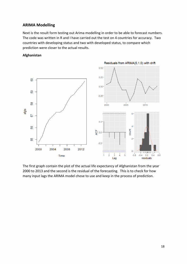
Next is the result form testing out Arima modelling in order to be able to forecast numbers. The code was written in R and I have carried out the test on 4 countries for accuracy. Two countries with developing status and two with developed status, to compare which prediction were closer to the actual results.
Afghanistan
The first graph contain the plot of the actual life expectancy of Afghanistan from the year 2000 to 2013 and the second is the residual of the forecasting. This is to check for how many input lags the ARIMA model chose to use and keep in the process of prediction.

19
The plot that the ARIMA model had forecast were 60.29 for the year 2014 and 60.68 for the year 2015. The actual record from the data were 2014 = 59.9 and 2015 = 65. The purple visualisation within the plot shows the lo and high 80 and 95 interval of which the age can fall under. The actual number can be view in R under the code print(forecasting). From this test you can see that the ARIMA does a fairly good job predicting numbers for the year 2014 but not that good for the year 2015 as it was about 5 years off. The ETS model did not do that much better having prediction score of 60.3 for 2014 and 60.66 for 2015. Judging from that however you can see that the ARIMA modelling result were closer to the actual figure than the ETS, as to be expected because the data here is quite stationary. Which is better suited to ARIMA.

20
Thailand
Result of ARIMA modelling prediction for the country Thailand, the second developing country used. The data had no value for the year 2015 so, only the value for the year 2014 were forecasted. The ARIMA model = 74.76 while the ETS model = 74.97 and the actual life expectancy for that year was 74.6 and again just like Afghanistan, the ARIMA was closest to the actual data. (Input lag used by ARIMA here was 4 again)

21
Ireland
The first developed country use for the prediction was Ireland and here unlike the last two ARIMA decided to only keep 3 input lags during prediction. The ARIMA forecast result are as 81 years old for both 2014 and 2015. ETS Model were 82.08 for both 2014 and 2015, while the actual data are 81.2 and 81.4. Again, the ARIMA modelling were closer to the correct figure, but if you notice here the lo and high interval are much larger than the previous two. This is presumably because of the fluctuation in data from 79.7 to 86

22
between 2009 and 2010, and the jump back down from 85 to 81 in 2012 and 2013. The ARIMA model did not have sufficient data to work with in forecasting so it generate a much larger possibility of what the life expectancy could be. What I meant by not enough sufficient data means ARIMA model does better with roughly 30 numbers of past data to use when predicting future number. But in our case, we only have about 12 or 13, this mean the result is not as accurate as it can be.
Canada

23
The second develop country that was used to for the ARIMA model testing was Canada, and here it chose to keep 5 input lags for the prediction. The result is very similar to that of Ireland as here there is also a lot of fluctuation within the data of life expectancy in each year. The ARIMA model predict 81.65 for 2014 and 81.56 for 2015, ETS model predict 81.78 for both years. The actual data are 82 for 2014 and 82.2 for 2015, this is the first result where the ETS model predict the closer result to the actual data. This could be because the ARIMA model had use more input lag than the last three or that the data fluctuates too much, and an accurate prediction could not be made from only these 13 inputs. By fluctuate too much, it may have impacted the stationary side of the data making it much better to use ETS modelling in this case.
The result of this determine that the ARIMA model is a fit datamining tool to use in forecasting numbers of future life expectancy as shown here. It is safe to assume that if I were to calculate for the year that this dataset did not provided, I would be able to calculate a close estimate of the actual result even the setback. And if there were to be new data readily available now of life expectancy from the year 2000 to 2021, I would be able to come up with an even better prediction with the technique practice here. From the result acquire from SPSS, it would also be safe to assume that if the dataset had more variables to input, I would be able to find out a more accurate number of which variables had a better percentage of predicting life expectancy. It should be fair to point out again that the ARIMA model would have worked better if there were more 30 or more data available to use per countries. This resulted in the prediction forecast graph output above and should be noted that the ARIMA model is not the issue but rather the lack of sufficient data.

24
6.0 Conclusions In conclusion I believed that the project had done well as I managed to at least answer the question that I set out to answer. Which was to understand the data better and figure out which factors plays a role in life expectancy around the world, I also managed to carry out a data mining technique to predict future numbers based on the data that I had despite the disadvantage of using such technique on this data. The results acquired from SPSS confirm what I had already suspected in which of the factors available within this dataset would be the one that had great dominance in affecting life expectancy. The prediction number forecasted had a close accuracy with the real figure, even though none of them were on the dot I believed if I had time to test it for every country that at least one of them would be. I had successfully acquired a table to represent and explain which contributing factor had an impact on the value of life expectancy and to what degree. Not only that but I had also a testing to confirmed if that factor being a contributor to the number was valid or not.
The advantage and strength of this project has to be how easy it was to navigate and analyse the dataset using R and SPSS. Both of these programs were taught in detail throughout the years along with tests and technique that you could perform on them to bring out result that you needed. Plus, since R and SPSS are widely known and used by data analysis all over the world, there were many online sources and materials I could look up and research to practice while carrying out this project. It was also an advantage because almost every module I had this year is dedicated to either data analyses or data mining.
The biggest limitation to this project is the lack of sufficient data to be able to use for data mining. While there are many variables and factors of data at my disposal, the most crucial one was the life expectancy number themselves. By having only about 14/15 data per countries really budget the accuracy of the prediction as ARIMA usually work wells with a minimum of 30 past data. If there just a little bit more life expectancy value say from 1980 to 2015, I would have had a much more accurate graph and results. The second thing was code knowledge of R, as I only began learning at the beginning of 4th year. I had limited knowledge on what I could do, and which packages R has that would have benefitted me. Likewise with SPSS, as I had only learned about and started using this year. The final limitation I believed that impacted the project is the time we are in, as the pandemic has close us off from college utilities and connection. Missing out on certain resources that otherwise could have positive effect on the project.
But overall, I’m glad the project turned out the way it did as I had gained more knowledge about the dataset and discovered a great tool to use in the future when dealing with prediction and forecasting.

25
7.0 Further Development or Research With additional time and research, I believed I could have made this project way better that what it currently is. I would spend more time in gather of the perfect data that contain sufficient amount of what I needed to perform the test again. I would also seek out to learn more about the ARIMA modelling and its overall design. As there were some figure and number that I still do not understand and R automatically calculated for me, if I had learned about it much more may I could have made a much better forecast even with the limited amount of data. Also, with more time and if my sole focus were to be worked on this project, I would study up on many more datamining technique to be able to use to extract other knowledge that I can from this dataset. There may be more trends and patterns that cannot be acquire from the analysis that I have used in this project, who know what more can we learned from this dataset.
There were a few theories that I tried to do within SPSS and R (still visible in R code submitted) that if I had time and more skill, I believed would yield interesting result. But I did not have the right tool and skillset at the current time to be able to bring out what is in my head onto the screen. Given more time I would definitely look into it a bit more.
Another thing I wanted to do if given more time was to incorporated python into this project somehow, as toward the end of the college year I briefly started to pick up and learned a bit of python. I realised that python code was easier to use and could have produce a much better visualisation of data than R. R is good in its own right, but I feel R is only better if you are an advance level of user that has been using R for a long time and not only started learning it for under a year. In the case of python, I think given enough time to use like R the end result could be much more pleasing, and the result may have also been better. This is due to the fact that python has a much bigger fanbase and usage, at least more than R. Judging from my research when doing this project.
If I got more time to pursue this project under python, I may have changed the aim of this project from building a prediction model to trying to understand the dataset better instead. Outputting various amount of graph and visualisation that python is capable of. Instead of forecasting graph, there may be a vast number of different factors from the dataset as chart of histogram along with explanation of what they do and how they affect other variables. Something along that line.
However, I will continue to study data analysis in this matter as I enjoyed the use of SPSS and R for analysation. I started seeing how this could be practical in the real world and why people choose to do them. It was interesting to think that I myself extract that bit of information from a dataset from a third-part website, and four year ago that sort of thing would have never enter my mind. Going forward I will still try to learn more and use more of these technique on data either in my free time or going into this kind of job.

26
8.0 References Moodle Slide from NCI lecturer – Advance Business Data Analysis, Data and Web mining, and Business Data analysis.
Data sources from WHO and acquired from Kaggle.com a third-party website that provide free and open dataset.
Zakaria Jaadi (2021) A STEP-BY-STEP EXPLANATION OF PRINCIPAL COMPONENT ANALYSIS (PCA), Available at: https://builtin.com/data-science/step-step-explanation-principal-component-analysis
RAINERGEWALT (2021) PCA vs Linear Regression – Therefore you should know the differences, Available at: https://starship-knowledge.com/pca-vs-linear-regression.
www.youtube.com. (n.d.). How to Use SPSS: Standard Multiple Regression. [online] Available at:
https://www.youtube.com/watch?v=f8n3Kt9cvSI&ab_channel=TheRMUoHPBiostatisticsResourceCh
annel [Accessed 1 May 2021].
Hyndman J. R and Athanasopoulos, G. “Forecasting: Principle and Practice”. Available at:
https://otexts.com/fpp2/
Markos, O. “Time Series Forecasting SARIMA vs Auto Arima models”. Available at:
https://medium.com/analytics-vidhya/time-series-forecasting-sarima-vs-auto-arima-models-
f95e76d71d8f#:~:text=ARIMA%20is%20a%20model%20that,future%20points%20in%20the%20serie
s.&text=MA(q)%20stands%20for%20moving,with%20time%20series%20with%20seasonality.
Chen, J. “Autoregressive Integrated Moving Average”. Investopedia. Available at: https://www.investopedia.com/terms/a/autoregressive-integrated-moving-average-arima.asp#:~:text=An%20autoregressive%20integrated%20moving%20average%2C%20or%20ARIMA%2C%20is%20a%20statistical,or%20to%20predict%20future%20trends.
Ruger JP, Yach D. The Global Role of the World Health Organization. Glob Health Gov. 2009;2(2):1-11.

27
9.0 Appendices This section should contain information that is supplementary to the main body of the report.
9.1. Project Plan Explain briefly within the Project proposal below.
9.2. Ethics Approval Application (only if required) Ethic Approval not required.
9.3. Reflective Journals

28
October Reflective Journal
Punnavit Kaewhin- BSHTM – X17713929
During the months of October, I have been researching data and content for Idea to pitch for the modules. I had look up data for road law, crime rate, gun law, diabetes, and mental health issues. In the end I had decided to go with the mental health issues as I felt it had the most relevance here in Ireland. In my mind I think that if the project work successfully it will be beneficial to a lot of people and sector. But I have to cover all the basis as it is a touchy subject and not ethic if I do it incorrectly. Overall, I think it is what I wanted to do but I also have a few backup data ideas in case. As my supervisor has got back to me that it may be difficult to cover some aspect of it. I had also check other website like WHO, OECD and World Bank to look for primary data if I should go ahead with this topic.
November Reflective Journal
During the months of November, I was tinkering around with SPSS and R to see how they worked. This is because R is now being taught in one of my modules and was told to be one of the main programs that we could use within our final year project. I also written up a pitch for the proposal of my project to be presented to the examiner. Not much else was accomplished as I was busy working on CA and assignments for mid term submission for my other modules.
December Reflective Journal for Software Project
Throughout December was the most progressive the project had been in the last 3 months. I’ve managed to input the dataset into R Studio to create graph and statistical facts from the data. I’ve stored this data into smaller sets for future work when I need to recall certain sets. Now I’ve created a good amount of smaller dataset from my main set and ordered them by categorically (E.g., Years, Countries, etc.). Not all of them as this would take sometimes, but a good few enough to merge or contrast with new dataset. I’ve also made a presentation slide for the submission, just to explained what my project is and what the final end product would look like. This will come in handy going forward and learning new thing in semester two.
All of this work was then noted down and filled into the report and explained on the mid-point submission videos. This month was the most challenging as there was many other module submissions and work as well. So, time management was something that was taken carefully. This month is also the one of the biggest months of contribution toward the project, as I’m starting to grasp what to do with R Studio and how I can used it to transform my dataset into something better.

29
Reflective Journal for January
This month involves a few searches for relevant data to input into R and see if the information would match up and be able to use with the current one. I’ve also continued to code more categories for the current dataset but not much due to the modules end exam that took place in the first two weeks of the month.
I’ve also began to work on my profile for the project showcase and have been taking advise from one of my friends who had it done last years.
Reflective Journal for February
This month I’ve continue adding code onto R for testing after consulting with my project supervisor. After taking his suggestion of using which data mining technique to incorporate into the project, I’ve began my research on what it is and how they could be accomplished. I’ve also input the dataset into SPSS and begin running analysis that I had worked on for my advance database CA. In regard to the project, this month was solely focusing on the pre-processing and cleaning of data. I’ve done this by studying which package was suitable to import into R and that would make it is easier to get rid and re-arrange the dataset into something that I needed.
Reflective Journal for March
This was a very productive month as I began writing up the SARIMA model and ETS code that I would be using in the project. This is because of doing TABAs for my final two modules had given me first-hand experience in using these techniques there first before I had the code and knowledge to incorporate it into my own project.
I’ve also run test in SPSS such as normality test to check if the data set is normally distributed and other test that were taught in advance databases such Chi-square test, non-parametric test, ANOVA test, Kruskal-Wallis, Shapiro Wilks, and many more. Then picking which one I wanted to keep in my report based on the what the test shows and explained. I was also saving every output (graphs, histogram, QQ plot, etc) that was acquired from SPSS and R studio and adding them into the report. I’d also filled up the beginning of the report by a good bit and explaining in detail my methodology for this project.
Reflective Journal – April
During April, the main focus was finishing off the rest of TABAs that was due before going ahead and working more on the project and its analysis. After having a chat with my project supervisor, he’d suggested I checked out a few different types of data mining techniques that would help greatly with my analysis of the data. I ended up choosing one called SARIMAX, a type of time series forecast technique. This is to help me create a graph visualising the number of life expectancy in the future. I’m currently in the stage of researching how to perform it and its detail before doing it on my actual data. I’d also look into a bit of python and had plan to implement it into my project, only to get some of better visualisation. As I feel the graph and detail that Python output are more pleasing than that

30
of R studio, but R will still be the one that I do the most coding on. And lastly, I’ve been filling up a bit of my report of the early test results and analysis.

31
9.4. Proposal
National College of Ireland
Project Proposal
Life Expectancy Pattern
07/11/2020
BSHTM
Data Analytic
Academic Year 2020/2021
Punnavit Kaewhin
X17713929

32
Contents 10 Objectives .................................................................................................................................. 33
11 Background ............................................................................................................................... 33
12 Technical Approach ................................................................................................................... 33
13 Special Resources Required ...................................................................................................... 33
14 Project Plan ............................................................................................................................... 34
15 Evaluation ................................................................................................................................. 34

33
10.0 Objectives The objective to study and analyse the data on life expectancy (may include other relevant data to the subject that have an impact on condition of life) in a given time frame for the countries around the world. This is done to output the result in a readable format or chart that is easy to interpret. So, that if we wanted to use the data to either determine or predict the life expectancy in the future.
That is the main aim, to gather enough evidence in the number of life expectancy for each country and output a close estimate for the future. Second is to understand why and how the factors within the dataset an effect on the life expectancy have numbers.
11.0 Background As we move forward into the future new discoveries and invention are being discovered all the time. With this our standard of living is presumptive to go up as well and I find it very interesting as to how not more than 50 years ago in certain country, the average life expectancy was only 66 years old. Compared to now of around 80 years old, we have made a huge leap forward. I wanted to know what factors are contributing to this jump in life expectancy. As being someone who come from a “poorer” country with a lower quality of lives than Ireland, it will be fascinating to see the numbers of the factors involve and how much impact it has to be able to contribute to the life expectancy numbers.
By pursuing this project, I would be able to provide many data and information regarding induvial average life expectancy of each country. Along with the trends and pattern that it may or may not accompany it. This information could prove useful to researcher, doctors, teachers and so on. Another piece of information I want to acquire that I believe would prove beneficial is downward trends and pattern of the average life expectancy. As it is correct to assume that if certain country has upward pattern, that other countries would have downward patterns to. If not, the very least a steady or very low upward patterns. This information could be very useful to researcher who are focusing helping developing country.
12.0 Technical Approach The software will be written on the programming language R as it will be taught more in dept this year over other computing languages. The data will be sources from both primary source and secondary that was gather already. There will also be need of designing and creating a database for the data gather.
A datamining technique had to be chosen to conduct analysis on the dataset to extract as much knowledge as possible from the dataset. This is to look for trend and patterns within the dataset and show them out as graph or visualisation.
13.0 Special Resources Required Knowledge of data mining Techniques and Methodology, mid-level usage of R and SPSS, and a good dataset regarding the field the project is in.

34
14.0 Project Plan
15.0 Evaluation My hope is to do a series of mock test as I will not be performing this on real end users as that would be sensitive data and expert’s professional would need to be included. But just having enough mock results to interpretate it’s false and accuracy. I want to also have a graph or some sort of visualization to show the trend and pattern acquire from the dataset.
16-Nov 26-Nov 06-Dec 16-Dec 26-Dec 05-Jan 15-Jan 25-Jan 04-Feb
Task 1 (Research Data)
Task 2 (Code Writing)
Task 3 (Trial)
Task 4 (Research Data)
Task 5 (Code Writing)
Task 6 (More Trial)
Task 7 (Provisional)
Task 8 (Provisional)
Gant Chart Provisional
Start Date
Days to Complete