national traffic speeds survey i
TRANSCRIPT

DOT HS 811 663 August 2012
National Traffic Speeds Survey I: 2007

DISCLAIMER
This publication is distributed by the U.S. Department of Transportation, National Highway Traffic Safety Administration, in the interest of information exchange. The opinions, findings, and conclusions expressed in this publication are those of the authors and not necessarily those of the Department of Transportation or the National Highway Traffic Safety Administration. The United States Government assumes no liability for its contents or use thereof. If trade names, manufacturers’ names, or specific products are mentioned, it is because they are considered essential to the object of the publication and should not be construed as an endorsement. The United States Government does not endorse products or manufacturers.
Suggested APA Format Citation:
Huey, R., De Leonardis, D., & Freedman, M. (2012, August). National traffic speeds survey I: 2007. (Report No. DOT HS 811 663). Washington, DC: National Highway Traffic Safety Administration

i
Technical Report Documentation Page
1. Report No. DOT HS 811 663
2. Government Accession No. 3. Recipient's Catalog No.
4. Title and Subtitle National Traffic Speeds Survey I: 2007
5. Report Date August 2012 6. Performing Organization Code
7. Author(s) Huey, R., De Leonardis, D., Shapiro, G., and Freedman, M.
8. Performing Organization Report No.
9. Performing Organization Name and Address WESTAT, Inc.
10. Work Unit No. (TRAIS)
1650 Research Blvd. Rockville, MD 20850
11. Contract or Grant No. DTNH22-02-D-65121; TASK ORDER 6
12. Sponsoring Agency Name and Address National Highway Traffic Safety Administration Office of Behavioral Safety Research (NTI-131) 1200 New Jersey Avenue SE Washington, DC 20590
13. Type of Report and Period Covered Final November, 2006 – July, 2008
14. Sponsoring Agency
Code
15. Supplementary Notes Paul J. Tremont, Ph.D., Geoff Collier, Ph.D., and Randolph Atkins, Ph.D. were the NHTSA Project Officers. 16. Abstract A field survey was conducted during spring and summer 2007 to measure travel speeds and prepare nationally-representative speed estimates for all types of motor vehicles on freeways, arterial highways, and collector roads across the United States. Over 10 million vehicle speeds were measured at more than 700 sites included in the geographic cluster sample of 20 primary sampling units (PSUs). Each PSU was a city, county, or group of two or three counties representing combinations of regions of the United States, level of urbanization, and type of topography (flat, hilly, mountainous). Speeds were acquired on randomly drawn road segments on limited access highways, major and minor arterial roads, and collector roads. Speed measurement sites were selected in road segments with low, medium or high degrees of horizontal and vertical curvature or gradient. Overall, speeds of free-flow traffic on freeways averaged 64.7 mph and were approximately 11 mph higher than on major arterials, which at 53.6 mph were in turn about 7 mph higher than the mean speed of 46.9 mph on minor arterials and collector roads. Most traffic exceeded the speed limits. Nearly half of traffic on limited access roads and about 60% of traffic on arterials and collectors exceeded the speed limit. About 15% of traffic exceeded the speed limit by 10 mph or more on freeways, arterials and collector roads. Speeds of passenger vehicle size classes were generally higher than for medium trucks. Often, speeds of large trucks were higher than medium trucks, and in some circumstances, large truck speeds were higher than passenger vehicles.17. Key Words speed-related crashes, speed management, driving speeds, traffic safety, speed measurement
18. Distribution Statement Document is available to the public from the National Technical Information Service www.ntis.gov
19. Security Classif. (of this report) Unclassified
20. Security Classif. (of this page) Unclassified
21. No. of Pages 98
22. Price

ii
Table of Contents
Tables .................................................................................................................................. v
Figures............................................................................................................................... vii
Executive Summary ......................................................................................................... viii
1. Introduction and Background ..................................................................................... 1
2. Study Overview .......................................................................................................... 1
3. Sample Design ............................................................................................................ 2
3.1. Site Selection ...................................................................................................... 3
3.2. Phase I - Site Documentation .............................................................................. 3
3.2.1. Recruitment and Training ........................................................................... 3
3.2.2. Instrumentation ........................................................................................... 3
3.2.3. Site Characteristics Data Collection ........................................................... 4
3.2.4. Final Site Selection ..................................................................................... 6
3.3. Phase II - Speed Data Collection ........................................................................ 6
3.3.1. Recruitment and Training ........................................................................... 7
3.3.2. Instrumentation ........................................................................................... 7
3.3.3. Site Coordination ........................................................................................ 9
3.3.4. Data Collection ......................................................................................... 10
3.3.5. Data Transmission .................................................................................... 13
3.3.6. Data Quality Assurance ............................................................................ 13
4. Data Weighting and Sample Expansion ................................................................... 15
4.1 Primary Sampling Unit Weight ........................................................................ 16
4.2 Site Weights, Phase I ........................................................................................ 17
4.3 Adjustment for Site Length ............................................................................... 17
4.4 Phase I Non-Response Adjustment ................................................................... 17

iii
4.5 Site Weights, Phase II ....................................................................................... 18
4.6 Non-Response Adjustment for Non-Observed Sites, Phase II ......................... 18
4.7 Adjustment for Non-Observed Lanes ............................................................... 19
4.8 Balancing by Day of Week ............................................................................... 19
4.9 Trimming Large Weights .................................................................................. 19
5. Results ....................................................................................................................... 20
5.1 Road Class ........................................................................................................ 21
5.2 Time of Day ...................................................................................................... 24
5.3 Light Condition ................................................................................................. 26
5.4 Day of Week ..................................................................................................... 28
5.5 Horizontal Curvature ........................................................................................ 30
5.6 Vertical Curvature ............................................................................................. 32
5.7 Urbanicity ......................................................................................................... 34
5.8 Vehicle Length .................................................................................................. 36
5.9 Horizontal and Vertical Curvature .................................................................... 38
5.10 Horizontal Curvature and Vehicle Length ........................................................ 43
5.11 Vertical Curvature and Vehicle Length ............................................................ 51
5.12 Horizontal Curvature and Light Condition ....................................................... 57
5.13 Vertical Curvature and Light Condition ........................................................... 61
5.14 Vehicle Length and Light Condition ................................................................ 65
6. Conclusions ............................................................................................................... 70
References ......................................................................................................................... 72

iv
Appendices ........................................................................................................................ 73
Appendix A. Sample Design Logic .............................................................................. 74
Appendix B. Hi-Star Specifications and Manufacturer Validation .............................. 79
v
Tables
Table 1. Creation of PSU Weights Based on NMVCCS and TSS Sampling of PSUs ..... 16
Table 2. Percent of Weights That Were Trimmed ............................................................ 20
Table 3. Overall Speeds by Road Class (All Traffic) ....................................................... 21
Table 4. Overall Speeds by Road Class (Free-Flow) ........................................................ 22
Table 5. Standard Deviations for the Values Reported in Table 3 and Table 4 ............... 23
Table 6. Proportion of Traffic Exceeding Speed Limit by Road Class (All Traffic) ....... 23
Table 7. Proportion of Traffic Exceeding Speed Limit by Road Class (Free-Flow) ........ 24
Table 8. Speed by Road Type and Time of Day (Free-Flow) .......................................... 25
Table 9. Standard Deviations for the Values Reported in Table 8 ................................... 26
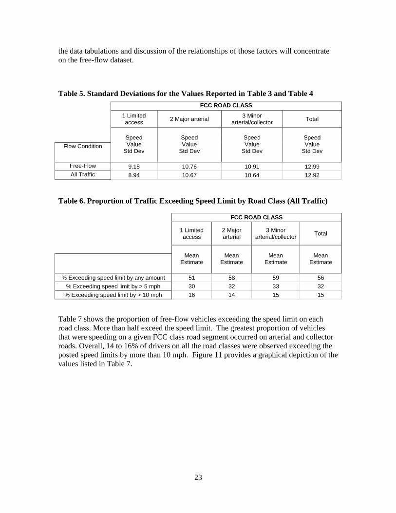
Table 10. Speed by Road Type and Light Condition (During May/June 2007) (Day=6 a.m. to 9 p.m. Night=9 p.m. to 6 a.m.) (Free-Flow) .................................... 27
Table 11. Standard Deviations for the Values Reported in Table 10 ............................... 28
Table 12. Speed by Road Type and Day of Week (Free-Flow) ........................................ 28
Table 13. Standard Deviations for the Values Reported in Table 12 ............................... 30
Table 14. Speed by Road Type and Horizontal Curvature Class (Free-Flow) ................. 30
Table 15. Standard Deviations for Values Reported in Table 14 ..................................... 31
Table 16. Speed by Road Type and Vertical Curvature Class (Free-Flow) ..................... 32
Table 17. Standard Deviations for Values Reported in Table 16 ..................................... 33
Table 18. Speed by Road Type by Urbanicity (Urban, Urban/Suburban, Suburban, Rural) (Free-Flow) .................................................................................................... 34
Table 19. Standard Deviations for Values Reported in Table 18 ..................................... 35
Table 20. Speed by Road Type by Vehicle Length Class (<10, 10-19, 20-29, 30-39, 40-59, 60-79, 80-99, >100) (Free-Flow) ................................................................... 36
Table 21. Standard Deviations for Values Reported in Table 20 ..................................... 38

vi
Table 22. Speed by Road Type, Horizontal Curvature Class, and Vertical Curvature Class. ......................................................................................................................... 39
Table 23. Standard Deviations for Values Reported in Table 22 ..................................... 42
Table 24. Speed by Road Type, Length Class, and Horizontal Curvature Class ............. 44
Table 25. Standard Deviations for Values Reported in Table 24 ..................................... 50
Table 26. Speed by Road Type, Length Class, and Vertical Curvature Class .................. 52
Table 27. Standard Deviations for Values Reported in Table 26 ..................................... 56
Table 28. Speed by Road Type, Horizontal Curvature Class, and Light Condition ......... 58
Table 29. Standard Deviations for Values Reported in Table 28 ..................................... 60
Table 30. Speed by Road Type, Vertical Curvature Class, and Light Condition ............. 62
Table 31. Standard Deviations for Values Reported in Table 30 ..................................... 64
Table 32. Speed by Road Type, Length Class, and Light Condition................................ 66
Table 33. Standard Deviations for Values Reported in Table 32 ..................................... 69
vii
Figures
Figure 1. Non-intersection Site Navigation Interface ......................................................... 4
Figure 2. Marking Documented Sites ................................................................................. 5
Figure 3. Site Documentation Interface .............................................................................. 5
Figure 4. Nu-Metrics Hi-Star (model NC-200) .................................................................. 8
Figure 5. Police Providing a Rolling Back-up for Hi-Star Installation............................. 10
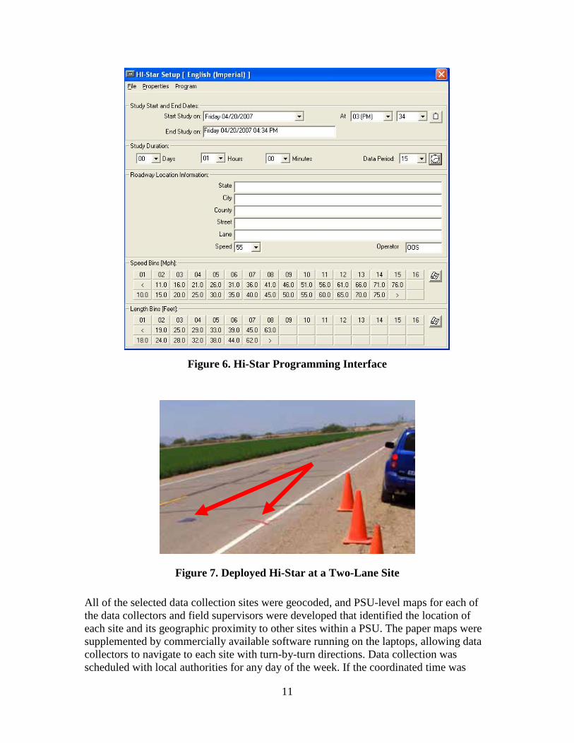
Figure 6. Hi-Star Programming Interface ......................................................................... 11
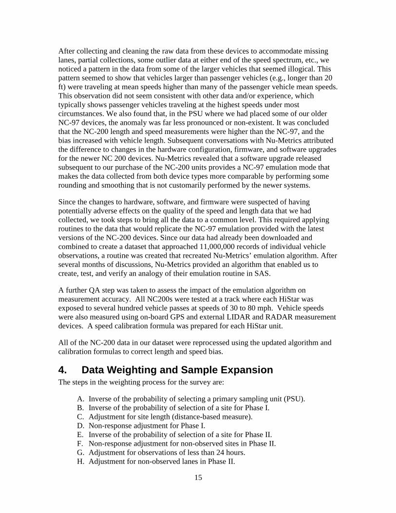
Figure 7. Deployed Hi-Star at a 2-Lane Site..................................................................... 11
Figure 8. Site Verification and Data Collection Documentation Interface ....................... 12
Figure 9. Hi-Star Deployment Schedule Tracking Interface ............................................ 13
Figure 10. Overall Speeds by Road Class ......................................................................... 22
Figure 11. Proportion of Traffic Exceeding the Speed Limit by Road Class ................... 24
Figure 12. Speed by Road Type and Time of Day ........................................................... 26
Figure 13. Speed by Road Type and Light Condition ...................................................... 27
Figure 14. Speed by Road Type and Day of Week........................................................... 29
Figure 15. Speed by Road Type and Horizontal Curvature Class .................................... 31
Figure 16. Speed by Road Type and Vertical Curvature Class ........................................ 33
Figure 17. Speed by Road Type by Urbanicity................................................................. 35
Figure 18. Speed by Road Type by Vehicle Length Class ............................................... 37
Figure 19. Speed by Road Type, Horizontal, and Vertical Curvature Class .................... 42
Figure 20. Speed by Road Type, Length Class, and Horizontal Curvature Class ............ 50
Figure 21. Speed by Road Type, Length Class, and Vertical Curvature Class ................ 56
Figure 22. Speed by Road Type, Horizontal Curvature Class, and Light Condition ....... 60
Figure 23. Speed by Road Type, Vertical Curvature Class, and Light Condition ............ 64
Figure 24. Speed by Road Type, Length Class, and Light Condition .............................. 69
viii
Executive Summary
The purposes of this project were to conduct a field survey to measure driving speeds for all types of motor vehicles on freeways, arterial highways, and collector roads across the United States and to produce national and regional estimates of travel speeds for various types of roads and vehicles.
A secondary objective was to explore the relationship between driving speeds and crashes on various classes of roadways. However, the required crash data were not available prior to the conclusion of this project; thus, we were unable to conduct this analysis. This report presents only the methods, findings, and conclusions of the speed survey.
The speed survey was designed as a geographic cluster sample of primary sampling units (PSUs), which can be a city, county, or group of two or three counties. PSUs were chosen to represent a range of combinations of regions of the United States, level of urbanization, and type of topography (flat, hilly, mountainous). Speeds were acquired on randomly drawn road segments on limited access highways, major and minor arterial roads, and collector roads. Speed measurement sites were selected in road segments with various degrees of straight, curved, flat, and hilly geometry. Twenty to 60 sites were selected in each PSU.
Sampling was done in two stages during the spring and summer of 2007. The first stage in the two-stage sampling approach selected a preliminary sample of sites in each PSU that was considerably larger than the actual quantity desired. All horizontal and vertical curve road segments, which are relatively rare compared to the more common straight and flat sections, were retained, while only a subsample of the more common situations were retained in the sample. Preliminary determination of rare and common site types was done using Geographic Information Systems (GIS) technologies. Measuring speed could be performed near, but not in an intersection. Determination of vertical curvature and gradient were possible only by field staff observation and measurement. Site documenters were equipped with global positioning satellite (GPS)-enabled laptop computers specially programmed with site location and curvature measurement routines to aid in determining which candidate sites to retain in the sample. This resulted in higher sampling rates for sites with “rare” characteristics and lower sampling rates for sites with “common” characteristics (e.g., local roads not near intersections and not on curves) than would have occurred with randomized selected means.
Speed data were collected during summer 2007. Speeds were measured using small, self-contained, on-road sensors (Nu-Metrics Hi-Stars) that Westat, Inc., data collectors temporarily placed on the road surface for a single 24-hour period at each road site.
The following are the principal findings and conclusions from the 2007 wave of the National Traffic Speeds Survey.

1. Mean, 85th percentile, and other measures of traffic speeds and speed variation for free-flow traffic compared to all traffic did not differ by more than 1.4 mph. About half of the observations were free-flow vehicles.
2. Overall, speeds of free-flow traffic on freeways averaged 64.7 mph and were approximately 11 mph higher than on major arterials, which at 53.6 mph were in turn about 7 mph higher than the mean speed of 46.9 mph on minor arterials and collector roads.
3. Standard deviation of free-flow traffic speed, a measure of the spread in the distribution of speeds, ranged from about 9 mph on freeways (14% of the mean) to 11 mph on minor arterials/collectors (23% of the mean).
4. More than half of free-flow traffic exceeded the speed limits. Nearly half of traffic on limited access roads and about 60% of traffic on arterials and collectors exceeded the speed limit. On freeways, arterials and collectors, 14 to 16% of traffic exceeded the speed limit by 10 mph or more.
5. Time of day had little influence on traffic speeds.
6. Period of light had little effect on travel speeds.
7. Mean speed differed by as much as 6 to 10 mph across day of week on major and minor arterials and collector roads, but by only 2 to 3 mph on freeways.
8. Speeds on straight sections of freeways and minor arterials/collectors were about 4 to 6 mph higher than on moderate curves, but horizontal curves had higher speeds on major arterials.
9. Speeds on flat sections of freeways were about 2 to 4 mph higher than on moderate or steep hills. Speeds on steep hills on minor arterials/collectors were about 5 to 6 mph lower than on flat or moderately hilly sections, while speeds on vertical curves on major arterials were 2 to 3 mph higher than on flat sections.
10. Speeds were lowest on urban roads and highest on rural roads of all types. Rural traffic was about 12 to 14 mph faster than urban traffic.
11. Speeds of passenger vehicle and light truck size classes (up to 29 ft.) were generally higher than for medium trucks (30 to 49 ft.). On all road types, speeds of large trucks (50 ft. or more) were higher than medium trucks, and in some circumstances, large truck speeds were higher than passenger vehicles.
12. There is an interaction among curvature (both horizontal and vertical), road class, and vehicle size. In general, speeds decrease as curvature and gradient increase, especially for the largest trucks on minor arterials/collectors.
13. There was little influence of light condition on speed across combinations of passenger vehicle size and road type. Nighttime speeds of the largest trucks were
ix

x
about 1 to 2 mph higher than during daytime on major and minor arterials, but were about the same day and night on freeways.
14. The sample design was less than optimal for estimating speeds. Because the design was a compromise to support both speed estimation and crash risk analysis, PSUs or sites within PSUs were not selected in a way that minimized error variance. A sample redesign should be considered for future waves to improve the speed estimates. The optimal design for general speed analysis is to have equal sampling rates and equal weights for every site. The over-sampling of crash sites resulted in a smaller sample of non-crash sites (assuming a fixed overall sample size) and differential weights between crash and non-crash sites, thereby increasing the variance for estimates that are not specific to crash sites.
15. The survey confirmed the feasibility of estimating travel speeds using a probability sample of measurement sites and uniform procedures for measuring speeds. More than 10 million observations of speeds were recorded of all vehicle types on freeways, major arterials and minor arterials and collector roads with various combinations of horizontal and vertical curvature.
16. The sub-study of the feasibility of measuring speeds at intersections where crashes occurred indicated that although speeds could be measured in each lane, damage and loss of measurement devices was substantially higher and risk of injury to field personnel was elevated at intersections, thus continuation of intersection measurements is not recommended.
1
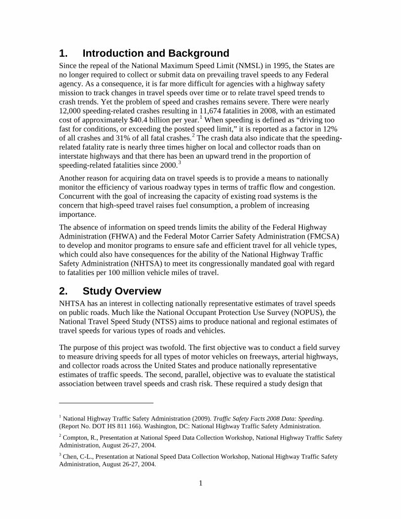
1. Introduction and Background Since the repeal of the National Maximum Speed Limit (NMSL) in 1995, the States are no longer required to collect or submit data on prevailing travel speeds to any Federal agency. As a consequence, it is far more difficult for agencies with a highway safety mission to track changes in travel speeds over time or to relate travel speed trends to crash trends. Yet the problem of speed and crashes remains severe. There were nearly 12,000 speeding-related crashes resulting in 11,674 fatalities in 2008, with an estimated cost of approximately $40.4 billion per year.1 When speeding is defined as “driving too fast for conditions, or exceeding the posted speed limit,” it is reported as a factor in 12% of all crashes and 31% of all fatal crashes.2 The crash data also indicate that the speeding-related fatality rate is nearly three times higher on local and collector roads than on interstate highways and that there has been an upward trend in the proportion of speeding-related fatalities since 2000.3
Another reason for acquiring data on travel speeds is to provide a means to nationally monitor the efficiency of various roadway types in terms of traffic flow and congestion. Concurrent with the goal of increasing the capacity of existing road systems is the concern that high-speed travel raises fuel consumption, a problem of increasing importance. The absence of information on speed trends limits the ability of the Federal Highway Administration (FHWA) and the Federal Motor Carrier Safety Administration (FMCSA) to develop and monitor programs to ensure safe and efficient travel for all vehicle types, which could also have consequences for the ability of the National Highway Traffic Safety Administration (NHTSA) to meet its congressionally mandated goal with regard to fatalities per 100 million vehicle miles of travel.
2. Study Overview NHTSA has an interest in collecting nationally representative estimates of travel speeds on public roads. Much like the National Occupant Protection Use Survey (NOPUS), the National Travel Speed Study (NTSS) aims to produce national and regional estimates of travel speeds for various types of roads and vehicles.
The purpose of this project was twofold. The first objective was to conduct a field survey to measure driving speeds for all types of motor vehicles on freeways, arterial highways, and collector roads across the United States and produce nationally representative estimates of traffic speeds. The second, parallel, objective was to evaluate the statistical association between travel speeds and crash risk. These required a study design that
1 National Highway Traffic Safety Administration (2009). Traffic Safety Facts 2008 Data: Speeding. (Report No. DOT HS 811 166). Washington, DC: National Highway Traffic Safety Administration. 2 Compton, R., Presentation at National Speed Data Collection Workshop, National Highway Traffic Safety Administration, August 26-27, 2004. 3 Chen, C-L., Presentation at National Speed Data Collection Workshop, National Highway Traffic Safety Administration, August 26-27, 2004.
2
supported access to detailed crash data, including pre-crash speeds, from a nationally representative sample of crashes with a well-defined sampling plan.
Development of national speed estimates and trends required a comprehensive, but economical, sample plan and field method to satisfy the requirements for collecting both speeds and the relationship between speeds and crashes. The recommended method was to use a cluster design similar to the annual NOPUS, which uses approximately 40 primary sampling units (PSUs) to estimate levels of safety restraint use on urban, suburban, exurban, and rural roads, or the National Automotive Sampling System (NASS), which uses a combination of PSUs where data collection methods are used to support estimates of crashes in the United States.
Note that the crash data for which the sample was designed were not available during the period of performance of this study, thus the speed-crash risk analysis was not performed. However, the estimates of speeds still have value for examining differences and trends for roadway and vehicle types and a variety of other travel observations.
For the 2007 NTSS, speeds were measured at 20 to 60 sites in each of 20 PSUs. Work was done in two phases during the spring and summer of 2007; a site documentation/selection phase followed by a speed data collection phase. Each PSU is a city, county, or group of two or three counties. PSUs were chosen to represent a range of combinations of regions of the United States, level of urbanization, and type of topography (flat, hilly, mountainous). Speeds were acquired on limited access highways, major and minor arterial roads, and collector roads. Speed measurement sites were selected in road segments with various degrees of straight, curved, flat, and hilly geometry. Self-contained, on-road sensors (Nu-Metrics Hi-Stars) were temporarily placed on the road surface for a single 24-hour period at each road site.
The sample in this study was not designed to support estimates of speeds for any specific State, county, or community. Consequently, data collection locations are not named in this report. The data are intended to be used by NHTSA to examine broad trends in speeds on various roadway types, by various vehicle types, etc.
3. Sample Design The sample design needed to accommodate and support a dual analytical requirement—to provide reliable national estimates of speeds and to determine the relationship between speeds and crashes. The intended analytical methodology involved regression analysis to generate speed distributions for a set of roadway sites and to match crashes that were associated with a combination of variables with estimated speed distributions for roads having a similar combination of variables. If speed causes crashes, then the speed when crashes occur is expected to be greater than the normal speed for matched roads. Since the crash risk analysis was never conducted, this report focuses only on estimation of speeds. However, for the interested reader, the logic behind the analytical approach and details of the design are presented in Appendix A.
3
3.1. Site Selection There were two defined phases in this study. Phase I involved identifying and documenting sites that were adequate for inclusion in the speed data collection conducted in Phase II. The site documentation visits were used to evaluate each site’s suitability in terms of traffic volume, surface type, location, road curvature, gradient, super elevation, drainage, and ability to safely deploy and retrieve data collection equipment. The second phase involved actually measuring the speeds along the selected roadways.
3.2. Phase I—Site Documentation A substantial oversample of sites was selected in each PSU, with the intent of obtaining data at all high curvature and high gradient sites but obtaining data only from a subsample of other sites. Data also could not be collected from sites where it was technically infeasible to place Hi-Stars at the site. The Phase II speed data collection is described in Section 3.3.
3.2.1. Recruitment and Training Recruiting site documenters was completed by drawing from a pool of field data collectors with proven skills necessary for completing this project. Site documenters needed to show proficiency in computer skills, reliability, and some potential for or past experience in management of data collection exercises in the field. This was important since they would ultimately serve as field supervisors for the speed data collection phase of the effort.
Training took place in two parts; the first involved a 2-day classroom tutorial, and the second took place on location at one of two PSU’s assigned to each site documenter. The classroom training included training on navigating to and surveying the sites, using the site documentation software to accurately record pertinent information regarding each site, proper field techniques, data transmission, and proper safety procedures for working on the side of the road. Trainers were TSS staff members with experience in conducting transportation field studies and using the site documentation equipment and software.
Project trainers then traveled with site documenters to one of their assigned PSU’s to complete the field training. Trainers and site documenters visited several of the proposed data collection sites in the PSU and worked together to document the sites and confirm the ability of the site documenter to work independently to gather information from the remaining sites. Once the trainers consistently observed that the site documenter’s work was proficient, site documenters were given full responsibility to complete the documentation effort for the remaining sites in their remaining PSU’s on their own and transmit the information electronically to Westat’s home office.
3.2.2. Instrumentation Each site documenter was assigned a laptop with a connected global positioning system (GPS), a digital camera, a safety vest, and a hard hat. A custom software application supported course navigation to each candidate site and then prompted documenters through each site to collect each of the needed data items for determining the site’s feasibility (see Figure 1). The GPS program provided directions to each of the sites and

4
collected horizontal and vertical roadway curvature data when driving through the site. A second program enabled site documenters to record information regarding roadway design and geometry for each site. The digital camera was used to snap several photos of each site. Photos provided first-hand views of the roadway and assisted in determining whether the site was appropriate for inclusion in the study. These photos also afforded the site documenters the opportunity to clearly identify any roadway characteristics that might lead to rejecting the site for speed data collection later in Phase II.
Figure 1. Non-Intersection Site Navigation Interface
3.2.3. Site Characteristics Data Collection Documenters were instructed to enter the candidate road segment at least ¼ mile in advance of the site. As they drove to within that ¼ mile radius, the PC with its GPS receiver began collecting curvature/elevation gradient data approximately every 100 feet, providing latitude and longitude as well as altitude data while the documenter drove past the site. Audible feedback was provided by the PC each time one of the samples was collected, when the site’s ¼ mile radius had been reached on the approach and retreat, and when the site center was reached.
After this drive-by step, the documenter returned to the center of the site and further documented the site during a walk-through. This step included taking several digital photos of the site, marking the road with paint to allow the speed data collector (during Phase II) to find the precise location at which the documenter would expect the Hi-Stars to be deployed, and providing written descriptions of the key aspects of the site for use in

5
final site selection. Figure 2 shows the road marking at a site, and Figure 3 shows the screen for documenting the walk-through information at a site.
Figure 2. Marking Documented Sites
Figure 3. Site Documentation Interface

6
Site documenters paid particular attention to several roadway characteristics:
·
·
·
·
·
Adequate separation from the site location to adjacent sources of traffic “friction” (traffic controls, intersections, driveways, uncharacteristic curves, congestion, etc.);
Paved roadway surfaces that would accommodate Hi-Star traffic classifiers with minimal chance of interference from overhead or underground sources of magnetic field disturbances;
Roadway delineation that would channel most vehicles directly over the Hi-Stars;
Surroundings that would promote safe installation and removal and likelihood that the Hi-Stars would survive a 24-hour installation (i.e., avoiding theft or destruction); and
Landmarks that would help an unaccompanied speed data collector find the site several weeks later.
At the end of each day, documenters uploaded data files with their observations from each site as well as digital photos taken at the site. The photos were electronically linked to the descriptive data files so all the information would be available for the final review and site selection at the home office.
For cases where the site was an intersection, a slightly different user interface was used to navigate and document the site. The intersection site interface included different color coding and fields for documentation of traffic control and driveway presence for both the cross road as well as the primary road. Once they completed documentation of intersection site, documenters were required to mark each of the lanes leading into the intersection for Hi-Star deployment in Phase II.
3.2.4. Final Site Selection As documentation data were received from the field, the documenter’s assessments of the feasibility of those sites were reviewed and given a final viability rating. This review included an appraisal of the completeness and consistency for a given site documentation exercise (e.g., was the “drive-by” documentation performed properly, were the street names and other requested characteristics provided, did the description match the photos, did the curvature data match the photos, etc.). It also included a rating of the site in terms of its feasibility with respect to the other candidates for that PSU. Sites that had some degree of curvature were intentionally selected for Phase II since sites with curvature or gradient were rarer than those with simple, straight trajectories.
3.3. Phase II—Speed Data Collection The second phase of data collection involved sending data collectors to the selected sites to coordinate with local authorities the installation and removal of Hi-Stars to collect speed data for 24 hours at each site.
7
3.3.1. Recruitment and Training Sixteen data collectors and several backup personnel were recruited from a pool of field staff to complete this phase of the study. As in Phase I, data collectors needed to show a certain level of proficiency with computers, a high degree of reliability and responsibility, and some potential or past experience in field data collection. Six field supervisors and 16 data collectors attended training. Because field supervisors had greater responsibility for supervising, managing, and assisting data collectors with questions about site locations and the use of the Hi-Stars, they attended an additional day of training to obtain the required expertise in equipment use, data downloading, site control, scheduling adjustments, and data collection quality control tasks. The supervisors’ other 2 days of training coincided with the field data collectors’ training.
Training involved an overview of the study’s purpose and its importance to highway safety; instruction on the programming, installation, and use of the Hi-Star devices; recharging and preparing all equipment for use in the field; methods for coordination with local authorities; use of custom software to document the data collection and verification of site information; procedures for transmitting data back to the home office; troubleshooting procedures for equipment, motorists, and coordination with the local enforcement officers; and safety techniques when working on the side of the road. Classroom work was followed by field practice where each of the 22 field workers was required to program, deploy, and retrieve a Hi-Star. These practice sessions included oversight by the project staff and the field supervisors so that each data collector received individual attention.
Field supervisors were instructed to make scheduled and unscheduled visits to each data collector to evaluate field performance. Each data collector was required to contact the field supervisor every night to report on the number of sites completed, data that had been submitted, any problems with data collection, etc. The field supervisors, in turn, contacted the field director each night to provide information on the status of each scheduled site and on their data collectors’ performance.
3.3.2. Instrumentation Similar to the site documentation in Phase I, data collectors were equipped with laptops and GPS receivers to help them navigate to the selected sites and perform quality control, verifying that data were collected at the appropriate locations. Each data collector was also given all of the equipment necessary to program and deploy 8 to 10 Nu-Metrics Hi-Stars. This included Hi-Star chargers, serial programming cables, Hi-Star covers, duct tape, and mastic tape.
Nu-Metrics Hi-Stars are small, self-contained devices that are placed on the roadway to both measure and store individual vehicle data for the vehicles that pass over them as the vehicles travel along road segments. The device uses magnetometers to measure the disturbance in the surrounding ambient magnetic field caused by the vehicles passage and then interprets speed and length (See Appendix B). They can be programmed to start and end data collection at specified dates and times. They are temporarily attached to road surfaces by tape or masonry anchors and left unattended for the period during which
8
observation is desired. After data collection is complete, they are retrieved from the roadway, and the data are read from the devices and stored in a database for analysis or transmission.
Hi-Stars were identified as the best choice for this data collection effort. At a minimum, the equipment selected for this study needed to be able to collect data on each individual vehicle in each lane in the traffic stream for at least 24 hours. To perform the required analyses, data needed to include individual vehicle speeds, vehicle type (cars, trucks, etc., based on length, wheelbase or number of axles), time of day, date, and separation time or distance between vehicles. Other alternatives, including road tubes, RADAR, LIDAR guns, side-fire RADAR, etc., were not chosen because of various limitations related to performing 24-hour simultaneous data collection in 2 to 10 lanes of traffic on a variety of road types. Road tubes would have required much more installation time and planning to allow multiple lanes to be captured and differentiated and would have been prone to destruction (i.e., breakage or movement), making their data unusable. RADAR and LIDAR were eliminated as possibilities because of their inability to discern multiple lanes and the need for manual supervision during the deployment over 24 hours.
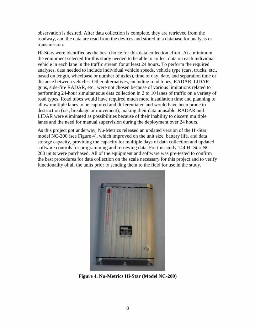
As this project got underway, Nu-Metrics released an updated version of the Hi-Star, model NC-200 (see Figure 4), which improved on the unit size, battery life, and data storage capacity, providing the capacity for multiple days of data collection and updated software controls for programming and retrieving data. For this study 144 Hi-Star NC-200 units were purchased. All of the equipment and software was pre-tested to confirm the best procedures for data collection on the scale necessary for this project and to verify functionality of all the units prior to sending them to the field for use in the study.
Figure 4. Nu-Metrics Hi-Star (Model NC-200)

9
Data collectors were also provided a database to store the information included in the nightly reports and any other details regarding contact that took place between the home office and field staff. This standard reporting protocol helped to quickly identify trends in data collection or field staff problems and support decisions with clear and concise information.
3.3.3. Site Coordination Coordinating with area police and other State officials for Phase II began months prior to the actual data collection. The NHTSA Contracting Officer’s Technical Representative (COTR) and NHTSA Regional Offices helped to identify PSU area police and other officials who could assist with traffic control during deployment and retrieval of the Hi-Stars in each PSU. Typically, several additional calls or e-mails from project staff at Westat or in the field were required to identify the authority responsible for managing the effort for any given roadway within a PSU as well as the individual responsible within that authority.
Immediately following their training, data collectors contacted each police jurisdiction to confirm the schedule for data collection in their areas. Any problems or special considerations for coordination were immediately directed to the home office.
Installation and removal of the device on surface streets normally required less than 1 minute on each lane. During a typical visit to a site, data collectors secured a Hi-Star to each lane in the selected roadway using strips of mastic tape or, in some cases, masonry anchors. Generally, both installation methods worked well, with losses due to theft or destruction relatively minimal, about 10% over the study duration. The assistance of the police or highway department jurisdiction responsible for the road was needed to control traffic for several minutes at each location for deployment and then 24 hours later for removal of these devices.
For arterials and collector roads, briefly stopping traffic in each lane let data collectors to affix the Hi-Stars. Removal required another brief stop of traffic. For limited access roads, Westat asked the State or county DOT to stop traffic briefly during installation and removal of speed measurement equipment on freeway lanes, typically using DOT vehicles with arrow boards and crash attenuators in temporary moving work zone configurations. In other cases, police created a slow rolling backup that provided a congestion buffer well upstream of the installation site to allow the data collector enough time to tape the devices to the road before traffic was allowed to resume. In either case, the process was much more complicated and involved greater coordination than the surface street installations.

10
Figure 5. Police Providing a Rolling Backup for Hi-Star Installation
3.3.4. Data Collection After coordinating an installation and removal time with local authorities, data collectors programmed each Hi-Star with information uniquely identifying where and when it was to be deployed. This information included State, city, county, roadway name, lane number and direction, speed limit, and start and end date and time for data collection (see Figure 6). After programming the Hi-Stars, each device was packaged to promote quick and proper installation/removal, minimizing the data collector exposure or impediments to passing traffic and to protect the unit from the elements during its deployment. It was also labeled with lane and direction information so that the data collector could easily identify which Hi-Star needed to be deployed in any given lane at a glance when deploying the units. Figure 7 shows one of the Hi-Stars deployed at a rural two-lane site. Note the red “X” left by the site documenter during Phase I to indicate the intended Hi-Star location during Phase II and the dark patch where the Hi-Star was secured to the road surface. Data collectors met police, sheriff, or highway department authorities capable of providing traffic control or diversion services for the period necessary for them to install and remove the Hi-Stars in each lane of a given site. Data collectors were usually able to stop or divert traffic with the assistance of the authorities and install or remove the Hi-Stars in a matter of a few minutes per lane.
11
Figure 6. Hi-Star Programming Interface
Figure 7. Deployed Hi-Star at a Two-Lane Site
All of the selected data collection sites were geocoded, and PSU-level maps for each of the data collectors and field supervisors were developed that identified the location of each site and its geographic proximity to other sites within a PSU. The paper maps were supplemented by commercially available software running on the laptops, allowing data collectors to navigate to each site with turn-by-turn directions. Data collection was scheduled with local authorities for any day of the week. If the coordinated time was

12
missed by the traffic control authorities (a frequent occurrence), rescheduling was required. Sites were rescheduled if there was adverse weather that would affect traffic speeds. Depending on the number of lanes being measured at a given site, a missed deployment appointment (due to a police emergency, bad weather, etc.) often meant several hours of delay before a new deployment time could be scheduled due to the requirement to pre-program and re-package the Hi-Stars before deployment could occur.
Similar coordination and traffic control was required again after 24 hours of data collection to remove the Hi-Stars. After retrieval of the Hi-Stars, the data collectors downloaded the information to their laptop computers and transmitted the data to Westat’s home office. Hi-Stars were recharged every night in preparation for data collection on the next day.
Custom software was developed to assist in the process of deployment and retrieval of the Hi-Stars to allow field supervisors and office staff to track the status of deployments and to determine if the data were being collected in a timely and complete fashion (see Figure 8 and Figure 9). For the data collectors, this provided a way to verify the information collected by the site documenters and a means to provide information about the collection status. Electronically tracking the status of each site ensured immediate access of the status data by office staff to allow reassignment of collection duties or re-collection in cases where data problems were recognized.
Figure 8. Site Verification and Data Collection Documentation Interface

13
Figure 9. Hi-Star Deployment Schedule Tracking Interface
3.3.5. Data Transmission Data collectors transmitted the electronic data files for each site back to the home office using a secure FTP server connection. After ensuring that the data had been received, data on the server were removed so that only databases located within the firewall held the transmitted information. Raw data residing on the data collector’s laptop was protected by usernames and passwords, which controlled not only access to the FTP server, but also access to the laptop user accounts.
3.3.6. Data Quality Assurance As data were transmitted from the field, raw data files were imported into databases for daily verification and cleaning. A variety of manual and automated queries performed on the data allowed for quick assessment of the data’s completeness as well as for determination of problems in the collection process. Every lane within a site was reviewed for the following descriptive statistics:
·
·
·
·
·
·
·
Sample size,
Mean and median speed,
Standard deviation,
Maximum and minimum speeds,
Percentile speeds (75th, 85th, and 95th),
Overall speed distribution, and
The presence of “phantom” vehicles.

14
Phantom vehicles were usually identified as vehicles with speeds of 0 mph or above 100 mph, as well as those vehicles with lengths of less than 0 feet or greater than 100 feet. When anomalies, such as high percentages of vehicles with 0 mph speeds or speeds greater than 100 mph, were identified within the raw data for any lane, data collectors were instructed to redeploy the units for a second round of data collection. Anomalies such as these were typically the result of Hi-Stars moving during data collection or vehicles side-swiping the unit. Sites were also revisited when specific anomalies were identified in any of the descriptive statistics (i.e., the mean speed of one lane was drastically different from the mean speeds of the other lane(s); sample sizes between lanes were drastically different; or there was an obvious failure of several of the Hi-Star units to collect data for the 24 hours. After the daily integrity checks were performed, the data collectors were allowed to move on to other sites or PSU’s.
Once data collection was complete in all PSUs, the raw data went through a more rigorous cleaning process and were merged with all of the descriptive information gathered during Phase I. Each lane within a site was cleaned separately. Each lane was reviewed for excessively high speeds (greater than 100 mph) and speeds of 0 mph, as well as a negative vehicle length or a length greater than 100 ft. If a vehicle met one of these criteria, it was considered a phantom vehicle and removed from the data set. In turn, the headway and gap measures were recalculated to reflect the new time differential between two consecutive vehicles. At this point, vehicles were also classified as free-flow vehicles, those with 5 seconds or greater difference between two consecutive vehicles, or not free-flow. Once the individual records were cleaned for each lane within a site, the number of hours when data were collected was calculated for each lane. Note that to be considered a good lane data set, the time between the first recorded vehicle and the last recorded vehicle in the lane had to be at least 16 hours. It was possible for no vehicles to be recorded during some hours, in which case the lane’s data were still considered good, even if up to 8 consecutive hours had no vehicle records (we assumed that this was likely due to no traffic on the road during that period rather than a malfunctioning Hi-Star). Further, at least one vehicle had to be recorded in each of 12 hours (not necessarily consecutive) for the lane data set to be considered good. Whenever both of those conditions were met, we accepted the data and made no form of weighting adjustment. However, if there were fewer than 16 hours between the first and last vehicle recorded or fewer than 12 hours with at least one vehicle observation in each hour, we deemed that likely due to a malfunctioning Hi-Star and treated the lane as “non-response.” In addition, lanes with an adequate number of hours with high percentages of vehicles with 0 mph speeds or high percentages of vehicles with excessively high speeds were also flagged as “non-response” lanes. Lanes identified as “non-response” were excluded from further data analyses.
Sites were categorized as “good” if usable data were collected from most of the lanes on the roadway as discussed in the previous paragraph.
There were some roadways where speed data collection was not completed due to weather conditions. For example, throughout most of the field data collection period, one PSU experienced a rainy season that prevented any deployment of the Hi-Stars.
15
After collecting and cleaning the raw data from these devices to accommodate missing lanes, partial collections, some outlier data at either end of the speed spectrum, etc., we noticed a pattern in the data from some of the larger vehicles that seemed illogical. This pattern seemed to show that vehicles larger than passenger vehicles (e.g., longer than 20 ft) were traveling at mean speeds higher than many of the passenger vehicle mean speeds. This observation did not seem consistent with other data and/or experience, which typically shows passenger vehicles traveling at the highest speeds under most circumstances. We also found that, in the PSU where we had placed some of our older NC-97 devices, the anomaly was far less pronounced or non-existent. It was concluded that the NC-200 length and speed measurements were higher than the NC-97, and the bias increased with vehicle length. Subsequent conversations with Nu-Metrics attributed the difference to changes in the hardware configuration, firmware, and software upgrades for the newer NC 200 devices. Nu-Metrics revealed that a software upgrade released subsequent to our purchase of the NC-200 units provides a NC-97 emulation mode that makes the data collected from both device types more comparable by performing some rounding and smoothing that is not customarily performed by the newer systems.
Since the changes to hardware, software, and firmware were suspected of having potentially adverse effects on the quality of the speed and length data that we had collected, we took steps to bring all the data to a common level. This required applying routines to the data that would replicate the NC-97 emulation provided with the latest versions of the NC-200 devices. Since our data had already been downloaded and combined to create a dataset that approached 11,000,000 records of individual vehicle observations, a routine was created that recreated Nu-Metrics’ emulation algorithm. After several months of discussions, Nu-Metrics provided an algorithm that enabled us to create, test, and verify an analogy of their emulation routine in SAS.
A further QA step was taken to assess the impact of the emulation algorithm on measurement accuracy. All NC200s were tested at a track where each HiStar was exposed to several hundred vehicle passes at speeds of 30 to 80 mph. Vehicle speeds were also measured using on-board GPS and external LIDAR and RADAR measurement devices. A speed calibration formula was prepared for each HiStar unit.
All of the NC-200 data in our dataset were reprocessed using the updated algorithm and calibration formulas to correct length and speed bias.
4. Data Weighting and Sample Expansion The steps in the weighting process for the survey are:
A. Inverse of the probability of selecting a primary sampling unit (PSU). B. Inverse of the probability of selection of a site for Phase I. C. Adjustment for site length (distance-based measure). D. Non-response adjustment for Phase I. E. Inverse of the probability of selection of a site for Phase II. F. Non-response adjustment for non-observed sites in Phase II. G. Adjustment for observations of less than 24 hours. H. Adjustment for non-observed lanes in Phase II.

16
I. Balancing for unequal distribution of assignments by day of week. J. Trimming of large weights.
Two sets of weights were produced. The first weight is for a “vehicle count” measure, and the second set is for a “distance-based” measure. The “vehicle count” measure is appropriate for estimating, for example, the mean speed of vehicles at a given instant in time or point along the road. It is not concerned with the distance that vehicles are traveling, and thus the length of an observation site does not figure into the weight.
The “distance-based” measure is appropriate for estimating the mean speed of vehicles according to the distance traveled by each vehicle. The length of an observation site must be included as a factor in the weighting. This measure is appropriate for describing total travel miles in relation to speed and is a more comprehensive representation of exposure to speed in everyday driving. Tables presented in this report are based on this distance-based measure.
The process is the same for the two weights, except for step C in the weighting (Section 4.3 below).
4.1 Primary Sampling Unit Weight We retained nearly all the PSUs that are in sample in the National Motor Vehicle Crash Causation Survey (NMVCCS). The inverse of the probability of selection for the 18 NMVCCS PSUs retained with certainty and the two subsampled PSUs is given in Table 1. We denote this weight as iP .
Table 1. Creation of PSU Weights Based on NMVCCS and TSS Sampling of PSUs
PSU
NMVCCS PSU weight
(NMVCCS_PSUWT)
Initial PSU conditional weight
(TSS_PSUWT)
Final PSU baseweight (PSU_BWT)
2 27.1 1 27.1 3 2.5 0 0 4 13 1 13 5 22.1 1 22.1 6 5.5 0 0 8 24.4 1 24.4 9 19.7 1 19.7 11 38.1 1 38.1 12 25.2 1 25.2 13 77.9 1 77.9 41 19 0 0 43 36.7 1 36.7 45 41.4 1 41.4 48 155.9 1 155.9 49 4.9 1 4.9 72 2.4 3.03 7.27 73 22 1 22 74 8.4 1 8.4
17
75 32.3 1 32.3 76 105.3 1 105.3 78 55.3 1 55.3 79 1.7 0 0 81 9.6 1 9.6
.
4.2 Site Weights, Phase I We consider only non-intersection sites, as intersection sites are not given weights. jiS ,,1 is the inverse of the probability of selection of the jth site in the ith PSU. Non-crash sites were selected with probability proportional to the length of the road segment. Crash sites for which speed or aggressive driving was indicated were sampled with certainty. Within each PSU, other crash sites were selected with equal probability.
The weight at this point in the process is jiW ,,1 = jii SP ,,1*
4.3 Adjustment for Site Length As discussed above, we have calculated two weights; each can be used for a separate set of tables. There may be additional weights used for specialized purposes at a later time. The first weight is a “count-based measure” that can be used to describe the average static vehicle density in relation to speed. The second weight, used in the set of tables in this report, is a “distance-based measure” that can be used to describe total travel miles in relation to speed. For the count-based measure, no additional adjustment is needed. For the distance-based measure, the weight is multiplied by the length of the site.
The distance-based weight is jjiji WW 1*' ,, = , where j1 is the length of the jth site.
4.4 Phase I Non-Response Adjustment Non-response adjustment was done for each of a number of non-response cells, using a weighting cell non-response adjustment methodology. Sites were considered to be non-response for reasons such as being unpaved or under construction. Roads that were closed to traffic during the study period, driveways, and roundabouts were considered as ineligible for the study. To determine cells where non-response rates differed, an analysis was done using a software package called CHAID (Chi-squared Automatic Interaction Detector) separately for crash sites and non-crash sites. The variables found by CHAID to be useful in defining cells with differential response rates were PSU, road class, total lanes, and curvy/high gradient (CG) status.
The non-response adjustment factor for a given cell is
1NR = [ å jiW ,,1 for respondents + å jiW ,,1 for non-respondents]/ [ å jiW ,,1 for respondents]. (Note that this is the adjustment factor for the count-based measure. The formula for the distance-based measure is the same, except jiW ,,1 is replaced by jiW ,,1¢ .)
18
The weight including this non-response adjustment factor is 1,,1,,2 * NRWW jiji = for the count-based measure and 1,,1,,2 * RNWW jiji ¢¢=¢ for the distance-based measure.
4.5 Site Weights, Phase II A subsample of eligible non-crash sites that are non-CG from Phase I was selected for actual data collection in Phase II, while all crash sites and other non-crash sites were retained with certainty. jiS ,,2 for a particular class of sites (crash, CG, non-CG) is the ratio of Phase I sites to selected Phase II sites.
The weight including this weight factor is jijiji SWW ,,2,,2,,3 *= .for the count-based measure and jijiji SWW ,,2,,2,,3 *¢=¢ for the distance-based measure.
4.6 Non-Response Adjustment for Non-Observed Sites, Phase II
An adjustment was made for sites not included in the estimates in two stages. First, there was a non-response adjustment for observations that could not be done in Phase II due to persistent rain or other bad weather conditions, inability to get police assistance, or because Westat ran out of time within the already extended field period to place the Hi-Stars. A CHAID analysis was again done to determine the definition of non-response cells. The variables found by CHAID to be related to the response rate and used in cell definition were PSU and total lanes.
The non-response adjustment factor for a given cell is 2N = [ å jiW ,,3 for respondents + å jiW ,,3 for non-respondents]/ [ å jiW ,,3 for respondents]
The weight, including this stage of non-response adjustment, is 2,,3,,4 * NWW jiji =
.for the count-based measure and 3,,3,,4 * NWW jiji ¢¢=¢ for the distance-based measure.
The second stage of the Phase II non-response adjustment was for sites where data were collected, but for which data were insufficient. A site was considered to be usable if less than half of the lanes were considered to be “non-responding” lanes. (Section 3.3.6 provides the details about when a lane was considered to be responding and non-responding.) Sites not meeting this criterion were regarded as non-responding. The non-response adjustment factor for non-responding sites due to lane data problems is
[ ] [ ]srespondentfor srespondent-nonfor srespondentfor 4443 ååå += ijijij WWWN
The weight, including this stage of non-response adjustment, is 345 * NWW ijij = for the count-based measure and 3,,4,,5 * NWW jiji ¢¢=¢ for the distance-based measure.

19
4.7 Adjustment for Non-Observed Lanes A non-response adjustment was made for non-responding lanes at sites that were considered as responding sites. A lane was non-responding according to the definition of response and non-response described in Section 3.3.6. We give an example of when a site was non-responding and a non-response adjustment was made as described in Section 4.6 and when a lane was non-responding and a nonresponse adjustment was made as described in this section. Suppose there are four lanes at a site. If three lanes were classified as non-responding, the site would be regarded as non-responding and the site non-response adjustment described in the preceding section would be applied. If, however, only one of the four lanes was classified as non-responding, the site would be regarded as responding, and there would be a non-response adjustment for only the bad lane.
A very simple lane non-response adjustment was made, in which data for the good lanes from a given site were given larger weights to account for the lanes lacking good data. For a given site, let R be the number of lanes for which there was good data, and let T be the total number of lanes at the site. The non-response adjustment factor is then T/R.
The weight including this adjustment factor is RTWW jiji *,,5,,6 = for the count-based
measure and RTWW jiji *,,5,,6 ¢=¢ for the distance-based measure.
4.8 Balancing by Day of Week Ideally, the same number of sites would be observed each day of the week. For a variety of reasons, this might not always be the case. To adjust for unequal number of observations between week days and the weekend, two factors were formed: 1D = 5/7*(weighted number total sites observed)/ (weighted number weekday sites observed) and 2D = 2/7*(weighted number total sites observed)/ (weighted number weekend sites observed). The factor 1D was applied to sites observed on weekdays and 2D was applied to sites observed on weekends. Weekend observations were defined as sites for which the placement of a Hi-Star occurred between 3 p.m. on a Friday and 3 p.m. on a Sunday, with weekday observations consisting of all other sites.
The weight, including this adjustment factor, is kjiji DWW *,,6,,7 = .for the count-based measure and kjiji DWW ¢¢=¢ *,,6,,7
4.9 Trimming Large Weights Very large weights lead to high sampling errors. Thus, we used normal Westat procedures for reducing the largest weights. Looking at all vehicle weights in CG sites, those weights that were more than 4.5 times the median weight for vehicles in this group as a whole were reduced to 4.5 times the mean weight. Similarly, looking at all vehicle weights in non-CG sites, those weights that were more than 4.5 times the median weight for the group as a whole were similarly reduced. However, we also avoided letting more than 5% of all vehicles have their weights trimmed. Thus, in some cases, weights that exceeded the threshold of 4.5 times the median were not trimmed, and in those situations,
20
weights were only trimmed back to the level of the largest non-trimmed weight. Trimming was done separately for the count-based weights and for the distance-based weights. Table 2, below, shows the percentages of weights that were trimmed.
TWW jiji *,,7,,8 = , where =T 1.0 for most vehicles and a value less than 1.0 for those vehicle weights requiring trimming.
'*'' ,,7,,8 TWW jiji = , where 'T is less than 1.0 for those vehicle weights requiring trimming
and 1.0 otherwise.
Table 2. Percent of Weights That Were Trimmed Curvy/ Non-curvy/
high gradient % low gradient % Count-based Crash sites 0 3.9
Non-crash sites .7 5.2 Distance-based Crash sites 1.3 7.1
Non-crash sites <.1 .9
The process of trimming slightly reduces the sum of total weights. Weights for all vehicles were slightly increased, separately for each of the four cells in Table 2, to restore the sum of weights prior to trimming. Let kF be the factor applied.
kjiji FWW *,,8,,9 = The final weights are
kjiji FWW *'' 8,,9 =
5. Results Tabulations of weighted speed estimates and standard error values are provided in the following pages. Table naming indicates the levels of road classification, daylight condition, time of day, day of week, horizontal or vertical roadway curvature, vehicle length, urbanicity, number of lanes, etc. that each tabulation represents. In each case, tables are presented in pairs, with mean, median, 85th percentile, and 95th percentile values in one table and immediately followed by a table with the standard deviations (SD) for the presented data. For all of the tables of results that follow, roadway classification uses the Functional Classification Code (FCC) definitions represented by those found in the Geographic Data Technology GDT database.
Several definitions are provided here to guide the reader through the presentation of these data. First, a standard error value is presented with each of the weighted values presented in the cross-tabulations. This standard error of the estimate represents the bounds of the 95% confidence interval for the presented weighted estimate (i.e., the weighted estimate for that cross-tabulation). The standard deviations, on the other hand, are presented as a companion table for each of the primary tables. These standard deviations provide a

21
measure of the spread of the un-weighted data above or below the un-weighted mean value. Note that we have not presented the un-weighted means in this report.
To avoid repetition in the discussion of the data, the reader should note that the data generally followed what we would expect to see for the FCC class breakouts. That is, FCC-1 (limited access highways) typically showed a higher overall speed than FCC-2 (major arterials). Likewise, FCC-2 road segments generally had higher speeds than most FCC-3 (minor arterials/collector) road segments. That said, the following results point out significant differences (or the lack thereof) for these and various other independent variables and combinations.
5.1 Road Class Overall speeds and proportions of vehicles exceeding the posted speed limit are presented for all traffic in Table 3 and for free-flow traffic in Table 4 to examine the extent of any difference between such flow regimes. In general, the speed estimates are quite comparable, with both typically falling within 1.4 mph of each other. Traffic speeds on limited access roads average about 11 to 12 mph faster than on major arterials, which in turn are 6 to 7 mph faster than on minor arterials and collector roads.
Table 3. Overall Speeds by Road Class (All Traffic)
FCC ROAD CLASS 1 Limited access 2 Major arterial 3 Minor arterial/collector Total
Speed Speed Speed Speed
Estimate Std Err Estimate Std Err Estimate Std Err Estimate Std Err Mean 64.45 0.67 52.39 1.59 46.43 1.27 54.93 1.04
Median 64.58 0.69 52.75 2.26 45.21 1.31 55.56 1.36 Quantile (0.85) 73.14 0.85 63.24 1.47 57.69 1.93 68.78 0.75 Quantile (0.95) 78.52 0.88 69.40 1.23 65.26 1.82 75.00 0.66
Table 4 shows the overall speed distributions by the three FCC classes under the free-flow conditions that will be considered from here forward in this report. Standard deviations are presented in Table 5. Despite the higher mean speeds, standard deviations for limited access roads were lower than for arterials or collectors. At about 12 mph on freeways, the standard deviation was about 16% of the mean, while for arterials and collectors, it was in the range of about 14 to 16 mph, or 25 to 30% of the mean. The 85th percentile values of these speeds range from about 9 to 12 mph above the mean, while the 95th percentiles are from about 12 to 19 mph above the mean. Figure 10 presents a graphic representation of the overall distribution of the free-flow traffic by road type.

22
Table 4. Overall Speeds by Road Class (Free-Flow)
FCC ROAD CLASS 1 Limited access 2 Major arterial 3 Minor arterial/collector Total Speed Speed Speed Speed Estimate Std Err Estimate Std Err Estimate Std Err Estimate Std Err
Mean 64.69 0.76 53.62 1.71 46.85 1.43 54.51 1.23 Median 64.86 0.79 54.10 2.22 45.85 1.62 55.02 1.66
Quantile (0.85) 73.77 0.73 64.46 1.38 58.30 2.09 68.48 0.92 Quantile (0.95) 79.20 0.79 70.64 1.28 65.95 1.69 75.06 0.77
Figure 10. Overall Speeds by Road Class (Free-Flow)
65
54
47
0
10
20
30
40
50
60
70
80
90
1 Limited Access 2 Major Arterial 3 Minor Arterial/Collector
95th percentile85th percentilemeanmedian15th percentile5th percentile
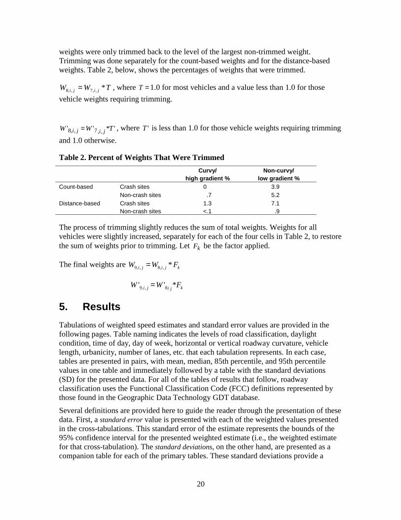
Table 5 provides the standard deviations of both datasets and again shows only a small difference in the values for free-flow versus overall traffic datasets. Likewise, the proportions of speeding vehicles shown in Table 6 and Table 7 were very similar for free-flow and overall conditions. For this reason, showing both sets of values for each tabulation was deemed unnecessary. Since the goal of this portion of the data collection effort was to determine the speeds chosen by drivers on given roadway classes as a function of various other independent factors, it seems prudent to concentrate on the portion of the data that represents drivers’ speed choices when not constrained by other drivers in proximity (i.e., under free-flow conditions). For that reason, the remainder of
23
the data tabulations and discussion of the relationships of those factors will concentrate on the free-flow dataset.
Table 5. Standard Deviations for the Values Reported in Table 3 and Table 4 FCC ROAD CLASS 1 Limited
access 2 Major arterial 3 Minor arterial/collector Total
Speed Value
Std Dev
Speed Value
Std Dev
Speed Value
Std Dev
Speed Value
Std Dev
Flow Condition
Free-Flow 9.15 10.76 10.91 12.99 All Traffic 8.94 10.67 10.64 12.92
Table 6. Proportion of Traffic Exceeding Speed Limit by Road Class (All Traffic)
FCC ROAD CLASS
1 Limited access
2 Major arterial
3 Minor arterial/collector Total
Mean
Estimate
Mean
Estimate
Mean
Estimate
Mean
Estimate
% Exceeding speed limit by any amount 51 58 59 56 % Exceeding speed limit by > 5 mph 30 32 33 32
% Exceeding speed limit by > 10 mph 16 14 15 15
Table 7 shows the proportion of free-flow vehicles exceeding the speed limit on each road class. More than half exceed the speed limit. The greatest proportion of vehicles that were speeding on a given FCC class road segment occurred on arterial and collector roads. Overall, 14 to 16% of drivers on all the road classes were observed exceeding the posted speed limits by more than 10 mph. Figure 11 provides a graphical depiction of the values listed in Table 7.

24
Table 7. Proportion of Traffic Exceeding Speed Limit by Road Class (Free-Flow)
FCC ROAD CLASS
1 Limited access
2 Major arterial
3 Minor arterial/collector Total
Mean
Estimate
Mean
Estimate
Mean
Estimate
Mean
Estimate
% Exceeding speed limit by any amount 48 60 61 56 % Exceeding speed limit by > 5 mph 28 34 35 33
% Exceeding speed limit by > 10 mph 14 15 16 15
Figure 11. Proportion of Traffic Exceeding the Speed Limit by Road Class
5.2 Time of Day There was very little variation in speeds by time of day, as shown in Table 8. The greatest variations appear to be on the smallest (FCC-3) roads, though the means were not significantly different across time periods. Figure 12 provides a graphic view of speeds by time of day.
Not Speeding: 52%Not Speeding: 40% Not Speeding: 39%
Exceeding Speed Limit by < 5 mph: 20%
Exceeding Speed Limit by < 5 mph: 26%
Exceeding Speed Limit by < 5 mph: 26%
Exceeding Speed Limit by 5-10 mph: 14% Exceeding Speed Limit
by 5-10 mph: 19%Exceeding Speed Limit
by 5-10 mph: 19%
Exceeding Speed Limit by > 10 mph: 14%
Exceeding Speed Limit by > 10 mph: 15%
Exceeding Speed Limit by > 10 mph: 16%
0%
10%
20%
30%
40%
50%
60%
70%
80%
90%
100%
1 Limited Access 2 Major Arterial 3 Minor Arterial/Collector

25
Table 8. Speed by Road Type and Time of Day (Free-Flow)
FCC ROAD CLASS
1 Limited access 2 Major arterial 3 Minor arterial/collector Total
Speed Speed Speed Speed TIMEDAY Estimate Std Err Estimate Std Err Estimate Std Err Estimate Std Err
1 Late night (0000-0559)
Mean 63.81 0.73 54.07 1.74 48.38 1.45 57.03 1.12 Median 63.87 0.68 54.06 2.47 47.62 1.87 58.00 1.29
Quantile (0.85) 72.64 0.70 64.55 1.68 60.00 1.62 69.37 0.66 Quantile (0.95) 77.97 0.76 71.33 2.27 67.29 1.38 75.42 0.68
2 Morning peak 3 hrs
(0600-0859)
Mean 65.15 0.79 54.45 1.83 48.06 1.50 55.11 1.16 Median 65.32 0.89 55.22 2.06 47.08 1.84 55.37 1.40
Quantile (0.85) 74.23 0.67 65.15 0.89 59.38 2.00 68.82 0.80 Quantile (0.95) 79.61 0.90 71.15 1.10 67.00 1.83 75.29 0.80
3 Mid-day 7 hrs
(0900-1559)
Mean 64.85 0.77 53.53 1.60 46.60 1.49 54.09 1.27 Median 65.00 0.87 54.00 2.01 45.49 1.50 54.60 1.81
Quantile (0.85) 74.00 0.79 64.38 1.38 58.16 2.20 68.18 0.95 Quantile (0.95) 79.33 0.87 70.61 1.30 65.73 1.87 75.00 0.92
4 Evening peak 3 hrs
(1600-1859)
Mean 65.07 0.84 54.02 1.91 46.89 1.52 54.03 1.35 Median 65.24 0.89 54.63 2.37 45.94 1.64 54.38 2.03
Quantile (0.85) 74.38 0.69 65.09 1.41 58.58 2.23 68.27 1.00 Quantile (0.95) 80.00 1.07 71.10 1.10 66.31 2.04 75.10 0.87
5 Early night 5 hrs
(1900-2359)
Mean 64.37 0.75 52.49 1.66 45.89 1.17 54.24 1.19 Median 64.54 0.73 52.75 2.35 44.74 1.22 54.64 1.70
Quantile (0.85) 73.40 0.82 63.19 1.63 57.00 1.87 68.34 0.88 Quantile (0.95) 78.65 0.77 69.52 1.34 64.56 1.62 74.98 0.92
Total
Mean 64.69 0.76 53.62 1.71 46.85 1.43 54.51 1.23 Median 64.86 0.79 54.10 2.22 45.85 1.62 55.02 1.66
Quantile(0.85) 73.77 0.73 64.46 1.38 58.30 2.09 68.48 0.92 Quantile (0.95) 79.20 0.79 70.64 1.28 65.95 1.69 75.06 0.77

26
Figure 12. Speed by Road Type and Time of Day
Table 9. Standard Deviations for the Values Reported in Table 8
FCC ROAD CLASS 1 Limited access 2 Major arterial 3 Minor art/collector Total
Speed Value
Std Dev
Speed Value
Std Dev
Speed Value
Std Dev
Speed Value
Std Dev
TIMEDAY
1 Late night (0000-0559) 8.82 10.33 10.90 12.03 2 Morning peak 3 hrs (0600-0859) 9.20 10.97 10.86 12.79 3 Mid-day 7 hrs (0900-1559) 9.13 10.74 10.95 13.09 4 Evening peak 3 hrs (1600-1859) 9.47 11.00 11.10 13.23 5 Early night 5 hrs (1900-2359) 9.03 10.48 10.50 13.01
Total 9.15 10.76 10.91 12.99
5.3 Light Condition Table 10 and Table 11 present daytime versus nighttime speeds and standard deviations. Since data were collected in May and June, daytime was defined as 6 a.m. to 9 p.m. Again, the differences are extremely small (i.e., 1 to 2 mph) between period of light
64 65 65 65 64
54 54 54 54 5248 48 47 47 46
0
10
20
30
40
50
60
70
80
901
Late
Nig
ht
(000
0-05
59)
2 M
orni
ng P
eak
3 Hr
s (0
600-
0859
)
3 M
id D
ay 7
Hou
rs
(090
0-15
59)
4 Ev
enin
g Pe
ak 3
Hrs
(1
600-
1859
)
5 Ea
rly N
ight
5 H
rs
(190
0-23
59)
1 La
te N
ight
(000
0-05
59)
2 M
orni
ng P
eak
3 Hr
s (0
600-
0859
)
3 M
id D
ay 7
Hou
rs(0
900-
1559
)
4 Ev
enin
g Pe
ak 3
Hrs
(160
0-18
59)
5 Ea
rly N
ight
5 H
rs(1
900-
2359
)
1 La
te N
ight
(000
0-05
59)
2 M
orni
ng P
eak
3 Hr
s (0
600-
0859
)
3 M
id D
ay 7
Hou
rs(0
900-
1559
)
4 Ev
enin
g Pe
ak 3
Hrs
(1
600-
1859
)
5 Ea
rly N
ight
5 H
rs(1
900-
2359
)
1 Limited Access 2 Major Arterial 3 Minor Arterial/Collector
95th percentile85th percentilemeanmedian15th percentile5th percentile
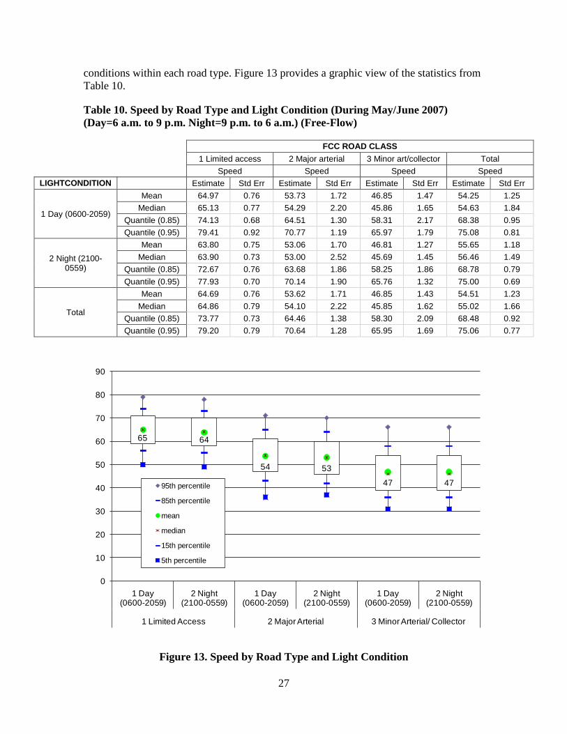
27
conditions within each road type. Figure 13 provides a graphic view of the statistics from Table 10.
Table 10. Speed by Road Type and Light Condition (During May/June 2007) (Day=6 a.m. to 9 p.m. Night=9 p.m. to 6 a.m.) (Free-Flow)
FCC ROAD CLASS 1 Limited access 2 Major arterial 3 Minor art/collector Total Speed Speed Speed Speed LIGHTCONDITION Estimate Std Err Estimate Std Err Estimate Std Err Estimate Std Err
1 Day (0600-2059)
Mean 64.97 0.76 53.73 1.72 46.85 1.47 54.25 1.25 Median 65.13 0.77 54.29 2.20 45.86 1.65 54.63 1.84
Quantile (0.85) 74.13 0.68 64.51 1.30 58.31 2.17 68.38 0.95 Quantile (0.95) 79.41 0.92 70.77 1.19 65.97 1.79 75.08 0.81
2 Night (2100-0559)
Mean 63.80 0.75 53.06 1.70 46.81 1.27 55.65 1.18 Median 63.90 0.73 53.00 2.52 45.69 1.45 56.46 1.49
Quantile (0.85) 72.67 0.76 63.68 1.86 58.25 1.86 68.78 0.79 Quantile (0.95) 77.93 0.70 70.14 1.90 65.76 1.32 75.00 0.69
Total
Mean 64.69 0.76 53.62 1.71 46.85 1.43 54.51 1.23 Median 64.86 0.79 54.10 2.22 45.85 1.62 55.02 1.66
Quantile (0.85) 73.77 0.73 64.46 1.38 58.30 2.09 68.48 0.92 Quantile (0.95) 79.20 0.79 70.64 1.28 65.95 1.69 75.06 0.77
Figure 13. Speed by Road Type and Light Condition
65 64
54 53
47 47
0
10
20
30
40
50
60
70
80
90
1 Day (0600-2059)
2 Night (2100-0559)
1 Day (0600-2059)
2 Night (2100-0559)
1 Day (0600-2059)
2 Night (2100-0559)
1 Limited Access 2 Major Arterial 3 Minor Arterial/ Collector
95th percentile
85th percentile
mean
median
15th percentile
5th percentile

28
Table 11. Standard Deviations for the Values Reported in Table 10
FCC ROAD CLASS 1 Limited access 2 Major arterial 3 Minor art/collector Total
Speed Value
Std Dev
Speed Value
Std Dev
Speed Value
Std Dev
Speed Value
Std Dev
LIGHTCONDITION
1 Day (0600-2059) 9.22 10.85 10.94 13.09 2 Night (2100-0559) 8.86 10.28 10.70 12.51
Total 9.15 10.76 10.91 12.99
5.4 Day of Week Variations attributable to the day of the week are presented in Table 12 and Table 13. On major arterials, mean speeds differed by day of week as much as 10 mph. On minor arterials and collectors the difference was smaller (6 mph), while freeway speeds showed little difference across day of week. Figure 14 provides a graphic view of the statistics from Table 12.
Table 12. Speed by Road Type and Day of Week (Free-Flow)
FCC ROAD CLASS 1 Limited access 2 Major arterial 3 Minor art/collector Total Speed Speed Speed Speed DAYWEEK Estimate Std Err Estimate Std Err Estimate Std Err Estimate Std Err
Mon
Mean 65.72 0.67 54.67 4.46 47.50 1.86 54.40 1.18 Median 66.00 0.90 55.37 4.07 46.85 2.41 54.78 1.57
Quantile (0.85) 75.06 0.81 65.07 2.11 58.58 2.54 68.06 1.97 Quantile (0.95) 81.00 1.29 71.07 1.12 65.00 1.62 75.10 1.77
Tue
Mean 64.68 1.67 52.12 1.39 47.16 3.80 55.41 2.29 Median 64.19 1.94 52.14 1.65 45.48 3.02 55.41 2.24
Quantile (0.85) 74.13 1.47 63.63 1.74 59.70 6.77 69.64 2.38 Quantile (0.95) 80.24 1.67 70.07 1.95 71.14 10.21 76.56 2.01
Wed
Mean 63.33 3.34 58.83 1.81 50.20 2.79 54.78 1.90 Median 63.39 3.42 58.92 1.76 49.48 3.07 55.22 2.11
Quantile (0.85) 73.49 3.93 65.81 0.22 62.35 3.95 67.07 1.92 Quantile (0.95) 79.42 4.01 70.14 2.53 70.18 4.09 74.08 2.56
Thu
Mean 65.63 1.60 54.80 4.22 44.17 1.34 49.89 1.85 Median 65.83 1.80 55.47 3.50 43.54 1.64 48.76 2.32
Quantile (0.85) 73.77 1.64 66.50 4.30 53.75 1.32 64.05 2.59 Quantile (0.95) 79.27 1.55 73.78 5.50 60.12 1.40 72.04 1.58
Fri
Mean 65.12 1.49 51.71 1.56 47.71 2.15 57.10 3.16 Median 65.27 1.07 50.72 2.26 46.98 3.32 58.58 4.36
Quantile (0.85) 73.27 0.98 62.21 2.61 59.97 2.76 70.02 1.86 Quantile (0.95) 78.06 1.31 69.32 2.52 66.32 2.55 75.57 1.51
Sat Mean 64.43 1.12 56.21 2.72 44.86 2.11 55.87 3.08
Median 64.22 0.81 56.38 2.04 43.51 2.49 57.45 3.62

29
FCC ROAD CLASS 1 Limited access 2 Major arterial 3 Minor art/collector Total Speed Speed Speed Speed DAYWEEK Estimate Std Err Estimate Std Err Estimate Std Err Estimate Std Err
Quantile (0.85) 73.64 1.27 65.71 1.48 56.17 3.41 69.92 2.33 Quantile (0.95) 79.32 1.65 72.12 2.16 63.17 2.67 76.37 2.16
Sun
Mean 63.26 3.30 48.84 4.39 45.75 2.92 51.34 2.25 Median 63.62 4.23 47.76 4.05 44.73 2.47 50.00 3.05
Quantile (0.85) 72.97 3.72 60.30 7.02 56.55 5.23 65.82 3.72 Quantile (0.95) 77.99 4.02 67.98 8.52 64.01 5.07 72.99 3.47
Total
Mean 64.69 0.76 53.62 1.71 46.85 1.43 54.51 1.23 Median 64.86 0.79 54.10 2.22 45.85 1.62 55.02 1.66
Quantile (0.85) 73.77 0.73 64.46 1.38 58.30 2.09 68.48 0.92 Quantile (0.95) 79.20 0.79 70.64 1.28 65.95 1.69 75.06 0.77
Figure 14. Speed by Road Type and Day of Week
66 6563
66 65 64 63
5552
59
5552
56
4948 47
50
4448
45 46
0
10
20
30
40
50
60
70
80
90
Mon Tu
e
Wed Th
u Fri
Sat
Sun
Mon Tu
e
Wed Th
u Fri
Sat
Sun
Mon Tu
e
Wed Th
u Fri
Sat
Sun
1 Limited Access 2 Major Arterial 3 Minor Arterial/ Collector
95th percentile
85th percentile
mean
median
15th percentile
5th percentile

30
Table 13. Standard Deviations for the Values Reported in Table 12
FCC ROAD CLASS 1 Limited access 2 Major arterial 3 Minor art/collector Total
Speed Value
Std Dev
Speed Value
Std Dev
Speed Value
Std Dev
Speed Value
Std Dev
DAYWEEK
Mon 9.70 10.93 10.49 12.91 Tue 9.19 10.92 12.15 13.16 Wed 9.78 7.39 11.53 11.97 Thu 8.40 11.82 9.40 12.68 Fri 8.30 9.92 11.34 12.56 Sat 9.05 9.81 10.47 13.39 Sun 10.06 10.62 10.08 12.72 Total 9.15 10.76 10.91 12.99
5.5 Horizontal Curvature Table 14 and Table 15 highlight the influence of horizontal curvature on speed for the road classes. The trends here are somewhat counterintuitive in that speeds on moderately curved segments of all road segments are 4 to 6 mph slower than straight segments, while speeds on sharply curved freeways, arterials and collectors are higher than on moderately curved segments. Figure 15 provides a graphic view of the statistics from Table 14.
Table 14. Speed by Road Type and Horizontal Curvature Class (Free-Flow)
FCC ROAD CLASS 1 Limited access 2 Major arterial 3 Minor art/collector Total Speed Speed Speed Speed
HOR_CURVERDCLASS Estimate Std Err Estimate Std
Err Estimate Std Err Estimate Std Err
1 Straight
Mean 64.89 0.68 53.32 1.69 47.63 1.41 55.03 1.22 Median 65.08 0.73 53.92 2.38 46.59 1.56 55.35 1.54
Quantile (0.85) 74.00 0.70 64.19 1.38 58.93 1.93 68.78 0.82 Quantile (0.95) 79.35 0.81 70.39 1.18 66.56 1.85 75.27 0.79
2 Moderate
Mean 60.57 4.40 58.97 2.61 41.11 1.96 47.73 2.60 Median 60.77 4.30 58.68 2.90 39.39 1.44 46.00 5.08
Quantile (0.85) 70.25 3.46 68.09 4.11 52.14 4.38 62.85 2.62 Quantile (0.95) 75.59 3.31 74.00 4.20 60.26 3.06 70.19 2.27
3 Sharp
Mean 63.87 3.61 59.23 . 42.04 2.93 53.04 6.69 Median 63.53 4.98 59.34 . 39.69 3.17 55.62 12.59
Quantile (0.85) 71.95 4.87 69.01 . 54.38 7.25 68.20 4.96 Quantile (0.95) 77.25 6.36 75.72 . 60.98 5.51 73.95 2.24
Total
Mean 64.69 0.76 53.62 1.71 46.85 1.43 54.51 1.23 Median 64.86 0.79 54.10 2.22 45.85 1.62 55.02 1.66
Quantile (0.85) 73.77 0.73 64.46 1.38 58.30 2.09 68.48 0.92 Quantile (0.95) 79.20 0.79 70.64 1.28 65.95 1.69 75.06 0.77

31
Figure 15. Speed by Road Type and Horizontal Curvature Class
Table 15. Standard Deviations for Values Reported in Table 14
FCC ROAD CLASS 1 Limited access 2 Major arterial 3 Minor art/collector Total
Speed Value
Std Dev
Speed Value
Std Dev
Speed Value
Std Dev
Speed Value
Std Dev
HOR_CURVERDCLASS
1 Straight 9.13 10.77 10.79 12.79 2 Moderate 9.52 8.95 10.06 13.29
3 Sharp 8.36 9.93 10.15 14.27 Total 9.15 10.76 10.91 12.99
6561
64
53
59 59
48
41 42
0
10
20
30
40
50
60
70
80
90
1 Straight
2 Moderate
3 Sharp
1 Straight
2 Moderate
3 Sharp
1 Straight
2 Moderate
3 Sharp
1 Limited Access 2 Major Arterial 3 Minor Arterial/ Collector
95th percentile
85th percentile
mean
median
15th percentile
5th percentile
32
5.6 Vertical Curvature Table 16 and Table 17 show the influence of vertical curvature gradient on the speeds for the road classes. Both moderate and steep gradients on freeways and minor arterials/collectors had speeds 2 to 6 mph slower than on level sections, but major arterials showed the opposite result for gradient. Figure 16 provides a graphic view of the statistics from Table 16.
Table 16. Speed by Road Type and Vertical Curvature Class (Free-Flow)
FCC ROAD CLASS 1 Limited access 2 Major arterial 3 Minor art/collector Total
Speed Speed Speed Speed VER_CURVERDCLASS Estimate Std Err Estimate Std Err Estimate Std Err Estimate Std Err
1 Flat
Mean 64.76 0.78 53.57 1.71 46.99 1.37 54.71 1.22 Median 64.98 0.88 54.04 2.19 45.97 1.47 55.22 1.51
Quantile (0.85) 73.93 0.73 64.46 1.37 58.37 1.93 68.69 0.86 Quantile (0.95) 79.33 0.86 70.56 1.12 66.00 1.86 75.23 0.79
2 Moderate
Mean 62.99 . 55.03 . 45.86 4.49 51.64 4.73 Median 62.69 . 55.39 . 43.49 4.52 52.78 8.17
Quantile (0.85) 70.39 . 59.72 . 59.30 8.31 64.98 4.67 Quantile (0.95) 75.07 . 62.71 . 65.13 6.22 70.50 4.89
3 Steep
Mean 61.01 . 56.25 13.67 41.47 3.56 46.08 4.71 Median 60.89 . 57.29 15.10 41.58 4.46 43.49 2.29
Quantile (0.85) 67.61 . 71.89 21.25 48.13 2.33 59.23 11.94 Quantile (0.95) 72.57 . 78.86 20.68 52.92 3.06 70.92 15.01
Total
Mean 64.69 0.76 53.62 1.71 46.85 1.43 54.51 1.23 Median 64.86 0.79 54.10 2.22 45.85 1.62 55.02 1.66
Quantile (0.85) 73.77 0.73 64.46 1.38 58.30 2.09 68.48 0.92 Quantile (0.95) 79.20 0.79 70.64 1.28 65.95 1.69 75.06 0.77
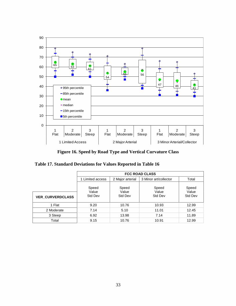
33
Figure 16. Speed by Road Type and Vertical Curvature Class
Table 17. Standard Deviations for Values Reported in Table 16
FCC ROAD CLASS 1 Limited access 2 Major arterial 3 Minor art/collector Total
Speed Value
Std Dev
Speed Value
Std Dev
Speed Value
Std Dev
Speed Value
Std Dev
VER_CURVERDCLASS
1 Flat 9.20 10.76 10.93 12.99 2 Moderate 7.14 5.10 11.01 12.45
3 Steep 6.92 13.98 7.14 11.89 Total 9.15 10.76 10.91 12.99
65 6361
5455 56
47 4641
0
10
20
30
40
50
60
70
80
90
1 Flat
2 Moderate
3 Steep
1 Flat
2 Moderate
3 Steep
1 Flat
2 Moderate
3 Steep
1 Limited Access 2 Major Arterial 3 Minor Arterial/Collector
95th percentile
85th percentile
mean
median
15th percentile
5th percentile
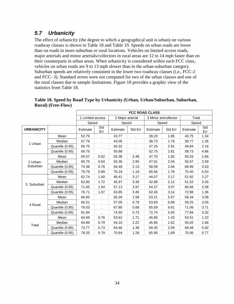
34
5.7 Urbanicity The effect of urbanicity (the degree to which a geographical unit is urban) on various roadway classes is shown in Table 18 and Table 19. Speeds on urban roads are lower than on roads in more suburban or rural locations. Vehicles on limited access roads, major arterials and minor arterials/collectors in rural areas are 12 to 14 mph faster than on their counterparts in urban areas. When urbanicity is considered within each FCC class, vehicles on urban roads are 9 to 13 mph slower than in the urban-suburban category. Suburban speeds are relatively consistent in the lower two roadway classes (i.e., FCC-2 and FCC- 3). Standard errors were not computed for two of the urban classes and one of the rural classes due to sample limitations. Figure 18 provides a graphic view of the statistics from Table 18.
Table 18. Speed by Road Type by Urbanicity (Urban, Urban/Suburban, Suburban, Rural) (Free-Flow)
FCC ROAD CLASS 1 Limited access 2 Major arterial 3 Minor art/collector Total Speed Speed Speed Speed
URBANICITY Estimate Std Err Estimate Std Err Estimate Std Err Estimate Std
Err
1 Urban
Mean 52.79 . 43.77 . 39.20 1.85 40.75 1.34 Median 57.79 . 43.05 . 38.73 1.76 39.77 1.35
Quantile (0.85) 65.75 . 50.32 . 47.25 2.91 49.84 2.16 Quantile (0.95) 69.75 . 55.88 . 52.75 2.81 58.73 4.86
2 Urban-Suburban
Mean 65.57 0.62 55.38 2.48 47.70 1.82 55.53 1.66 Median 65.75 0.64 55.36 2.95 47.01 2.04 55.67 2.59
Quantile (0.85) 74.38 0.76 64.49 2.13 58.59 2.64 68.96 0.53 Quantile (0.95) 79.79 0.89 70.19 1.19 65.56 1.78 75.40 0.53
3 Suburban
Mean 62.74 1.40 46.41 3.17 44.07 2.17 51.92 2.27 Median 62.85 1.72 45.97 3.30 42.89 2.12 51.52 3.35
Quantile (0.85) 71.65 1.04 57.13 3.97 54.27 3.07 66.66 2.08 Quantile (0.95) 76.71 1.07 63.85 3.45 62.45 3.14 72.98 1.36
4 Rural
Mean 66.65 . 56.26 1.58 53.21 5.57 58.34 3.08 Median 66.51 . 57.05 0.79 53.83 6.89 59.25 3.05
Quantile (0.85) 76.03 . 67.85 0.68 65.59 6.61 71.06 3.71 Quantile (0.95) 81.84 . 74.50 0.73 72.74 5.50 77.84 3.32
Total
Mean 64.69 0.76 53.62 1.71 46.85 1.43 54.51 1.23 Median 64.86 0.79 54.10 2.22 45.85 1.62 55.02 1.66
Quantile (0.85) 73.77 0.73 64.46 1.38 58.30 2.09 68.48 0.92 Quantile (0.95) 79.20 0.79 70.64 1.28 65.95 1.69 75.06 0.77

35
Figure 17. Speed by Road Type by Urbanicity
Table 19. Standard Deviations for Values Reported in Table 18
FCC ROAD CLASS 1 Limited access 2 Major arterial 3 Minor art/collector Total
Speed Value
Std Dev
Speed Value
Std Dev
Speed Value
Std Dev
Speed Value
Std Dev
URBANICITY
1 Urban 15.29 6.67 7.91 9.38 2 Urban-Suburban 8.96 9.17 10.53 12.56
3 Suburban 8.84 10.54 9.94 13.11 4 Rural 9.10 11.46 12.11 12.40 T
otal 9.15 10.76 10.91 12.99
53
6663
67
44
55
46
56
39
4844
53
0
10
20
30
40
50
60
70
80
90
1 U
rban
2 U
rban
-Su
burb
an
3 S
ubur
ban
4 R
ural
1 U
rban
2 U
rban
-Su
burb
an
3 S
ubur
ban
4 R
ural
1 U
rban
2 U
rban
-Su
burb
an
3 S
ubur
ban
4 R
ural
1 Limited Access 2 Major Arterial 3 Minor Arterial/Collector
95th percentile
85th percentile
mean
median
15th percentile
5th percentile

36
5.8 Vehicle Length Table 20 and Table 21 indicate the influence of vehicle length on speed for the various road classes. Vehicles in length classes 1 and 2 are passenger vehicles and light trucks; categories 3 and 4 are generally medium trucks, and classes 5 and 6 are heavy trucks/combination vehicles. Speeds of passenger size vehicles and light trucks were generally higher by 2 to 5 mph than for medium trucks on limited access and major arterial roadways. However, the largest vehicles were up to 7 mph faster than other vehicles on arterials and collectors. Figure 18 provides a graphic view of the statistics from Table 20.
Table 20. Speed by Road Type by Vehicle Length Class (<20, 20-29, 30-39, 40-49, 50-79, 80-100) (Free-Flow)
FCC ROAD CLASS
1 Limited access 2 Major arterial 3 Minor art/collector Total
Speed Speed Speed Speed
VEH_LENGTH Estimate Std Err Estimate Std
Err Estimate Std Err Estimate Std
Err
1 (<20 ft)
Mean 64.72 0.86 52.45 1.56 45.80 1.29 52.88 1.07
Median 65.08 0.93 52.75 2.15 44.74 1.23 52.63 1.72 Quantile
(0.85) 73.84 0.91 63.00 1.52 56.53 2.09 67.44 1.02
Quantile (0.95) 79.04 0.92 69.18 1.29 64.30 2.19 74.21 0.89
2 (20-29 ft)
Mean 67.08 0.73 58.59 1.69 52.75 1.71 60.10 1.08
Median 67.33 0.88 59.54 1.32 53.82 2.10 61.03 0.87 Quantile
(0.85) 76.41 0.87 68.91 0.75 64.48 1.16 72.67 0.69
Quantile (0.95) 81.80 0.96 75.22 0.90 71.87 1.42 78.62 0.65
3 (30-39 ft)
Mean 61.53 0.60 53.29 1.96 49.18 1.56 54.95 1.12
Median 61.38 0.75 54.51 2.43 49.30 2.84 55.50 0.68 Quantile
(0.85) 70.29 0.65 63.75 1.46 61.09 0.98 66.79 0.77
Quantile (0.95) 76.17 0.45 70.53 0.98 68.11 1.82 73.28 0.89
4 (40-49 ft)
Mean 60.24 0.88 53.59 1.59 49.60 1.77 55.17 1.02
Median 60.32 0.67 54.34 1.65 50.03 2.92 55.61 0.76 Quantile
(0.85) 68.89 0.66 63.60 1.08 60.43 1.15 65.95 0.46
Quantile (0.95) 74.41 0.83 69.60 1.88 66.70 1.35 71.90 0.68
5 (50-79 ft)
Mean 62.36 1.18 56.15 1.44 53.08 1.72 60.40 1.21
Median 62.48 1.18 56.86 1.45 54.16 2.51 61.03 1.00 Quantile
(0.85) 69.29 1.02 64.64 1.38 63.05 0.55 68.25 0.88

37
FCC ROAD CLASS
1 Limited access 2 Major arterial 3 Minor art/collector Total
Speed Speed Speed Speed
VEH_LENGTH Estimate Std Err Estimate Std
Err Estimate Std Err Estimate Std
Err Quantile
(0.95) 74.12 0.93 70.04 2.24 68.18 1.29 73.21 0.75
6 (80-100 ft)
Mean 66.54 1.58 61.71 1.41 57.18 2.78 65.43 1.39
Median 66.41 1.03 62.93 1.12 58.56 4.87 65.76 0.94 Quantile
(0.85) 74.18 1.82 70.23 4.15 68.56 3.30 73.68 1.53
Quantile (0.95) 80.05 2.56 75.03 4.42 72.72 2.47 79.53 1.97
Total
Mean 64.69 0.76 53.62 1.71 46.85 1.43 54.51 1.23
Median 64.86 0.79 54.10 2.22 45.85 1.62 55.02 1.66 Quantile
(0.85) 73.77 0.73 64.46 1.38 58.30 2.09 68.48 0.92
Quantile (0.95) 79.20 0.79 70.64 1.28 65.95 1.69 75.06 0.77
Figure 18. Speed by Road Type by Vehicle Length Class
65 6762 60
6267
52
59
53 5456
62
46
5349 50
53 57
0
10
20
30
40
50
60
70
80
90
100
1 (<
20 ft
)
2 (2
0-29
ft)
3 (3
0-39
ft)
4 (4
0-49
ft)
5 (5
0-79
ft)
6 (8
0-10
0 ft)
1 (<
20 ft
)
2 (2
0-29
ft)
3 (3
0-39
ft)
4 (4
0-49
ft)
5 (5
0-79
ft)
6 (8
0-10
0 ft)
1 (<
20 ft
)
2 (2
0-29
ft)
3 (3
0-39
ft)
4 (4
0-49
ft)
5 (5
0-79
ft)
6 (8
0-10
0 ft)
1 Limited Access 2 Major Arterial 3 Minor Arterial/Collector
95th percentile85th percentilemeanmedian15th percentile5th percentile

38
Table 21. Standard Deviations for Values Reported in Table 20
FCC ROAD CLASS 1 Limited access 2 Major arterial 3 Minor art/collector Total
Speed Value
Std Dev
Speed Value
Std Dev
Speed Value
Std Dev
Speed Value
Std Dev
VEH_LENGTH
1 (<20 ft) 9.32 10.45 10.41 13.01 2 (20-29 ft) 9.18 11.18 12.06 12.48 3 (30-39 ft) 8.91 10.95 11.51 11.82 4 (40-49 ft) 8.87 10.23 10.66 10.88 5 (50-79 ft) 7.16 9.17 10.11 8.57
6 (80-100 ft) 7.75 9.97 10.71 8.64 Total 9.15 10.76 10.91 12.99
5.9 Horizontal and Vertical Curvature Table 22 and Table 23 show cross-tabulations of the impact of various horizontal and vertical curvature categories within a roadway classification. There are a number of cells in Table 22 that have relatively low levels of site representation, limiting the statistical confidence in the estimated speed values expressed in the cross-tabulation. Generally, greater horizontal and vertical curvature is associated with lower speeds. The impact of vertical curvature on speeds is more prevalent on the smallest road classes (FCC-3). Unfortunately, the number of sites where there is a combination of these extremes is small, precluding more detailed analyses. Figure 19 provides a graphic view of the statistics from Table 22.

39
Table 22. Speed by Road Type, Horizontal Curvature Class, and Vertical Curvature Class.
FCC ROAD CLASS 1 Limited access 2 Major arterial 3 Minor art/collector Total
Speed Speed Speed Speed
HOR_CURVERDCLASS VER_CURVERDCLASS Estimate Std Err Estimate Std Err Estimate Std Err Estimate Std Err
1 Straight
1 Flat
Mean 64.89 0.68 53.25 1.69 47.73 1.32 55.24 1.18 Median 65.09 0.73 53.78 2.35 46.81 1.41 55.50 1.44
Quantile (0.85) 74.00 0.69 64.09 1.40 58.93 1.82 68.91 0.81 Quantile (0.95) 79.35 0.81 70.28 1.06 66.70 1.86 75.41 0.84
2 Moderate
Mean . . 55.03 . 45.84 6.60 47.04 7.56 Median . . 55.39 . 42.98 5.44 45.29 8.11
Quantile (0.85) . . 59.72 . 60.65 13.48 60.31 13.10 Quantile (0.95) . . 62.71 . 65.84 13.45 65.47 13.09
3 Steep
Mean 61.01 . 56.73 14.36 45.17 1.94 50.35 5.49 Median 60.89 . 57.69 15.27 44.70 1.21 46.52 2.90
Quantile (0.85) 67.61 . 71.92 21.35 50.41 2.24 63.85 12.72 Quantile (0.95) 72.57 . 78.87 20.71 54.96 2.92 73.98 14.29
Total
Mean 64.89 0.68 53.32 1.69 47.63 1.41 55.03 1.22 Median 65.08 0.73 53.92 2.38 46.59 1.56 55.35 1.54
Quantile (0.85) 74.00 0.70 64.19 1.38 58.93 1.93 68.78 0.82 Quantile (0.95) 79.35 0.81 70.39 1.18 66.56 1.85 75.27 0.79
2 Moderate
1 Flat
Mean 60.57 4.40 59.12 2.60 40.26 1.89 48.08 3.02 Median 60.77 4.30 58.70 2.96 38.66 1.08 46.57 6.16
Quantile (0.85) 70.25 3.46 68.11 4.11 50.48 5.17 63.48 2.87 Quantile (0.95) 75.59 3.31 74.01 4.17 59.58 4.22 70.84 2.37
2 Moderate
Mean . . . . 50.82 3.11 50.82 3.11 Median . . . . 50.64 3.17 50.64 3.17
Quantile (0.85) . . . . 59.54 4.13 59.54 4.13 Quantile (0.95) . . . . 64.77 3.77 64.77 3.77
3 Steep
Mean . . 33.10 . 36.89 3.86 36.81 3.70 Median . . 32.17 . 36.52 3.48 36.29 3.62
Quantile (0.85) . . 38.65 . 42.33 4.77 42.29 4.64 Quantile (0.95) . . 44.03 . 46.89 5.79 46.82 5.44
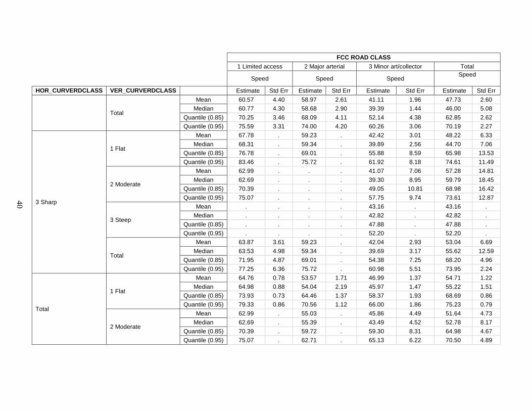
40
FCC ROAD CLASS 1 Limited access 2 Major arterial 3 Minor art/collector Total
Speed Speed Speed Speed
HOR_CURVERDCLASS VER_CURVERDCLASS Estimate Std Err Estimate Std Err Estimate Std Err Estimate Std Err
Total
Mean 60.57 4.40 58.97 2.61 41.11 1.96 47.73 2.60 Median 60.77 4.30 58.68 2.90 39.39 1.44 46.00 5.08
Quantile (0.85) 70.25 3.46 68.09 4.11 52.14 4.38 62.85 2.62 Quantile (0.95) 75.59 3.31 74.00 4.20 60.26 3.06 70.19 2.27
3 Sharp
1 Flat
Mean 67.78 . 59.23 . 42.42 3.01 48.22 6.33 Median 68.31 . 59.34 . 39.89 2.56 44.70 7.06
Quantile (0.85) 76.78 . 69.01 . 55.88 8.59 65.98 13.53 Quantile (0.95) 83.46 . 75.72 . 61.92 8.18 74.61 11.49
2 Moderate
Mean 62.99 . . . 41.07 7.06 57.28 14.81 Median 62.69 . . . 39.30 8.95 59.79 18.45
Quantile (0.85) 70.39 . . . 49.05 10.81 68.98 16.42 Quantile (0.95) 75.07 . . . 57.75 9.74 73.61 12.87
3 Steep
Mean . . . . 43.16 . 43.16 . Median . . . . 42.82 . 42.82 .
Quantile (0.85) . . . . 47.88 . 47.88 . Quantile (0.95) . . . . 52.20 . 52.20 .
Total
Mean 63.87 3.61 59.23 . 42.04 2.93 53.04 6.69 Median 63.53 4.98 59.34 . 39.69 3.17 55.62 12.59
Quantile (0.85) 71.95 4.87 69.01 . 54.38 7.25 68.20 4.96 Quantile (0.95) 77.25 6.36 75.72 . 60.98 5.51 73.95 2.24
Total
1 Flat
Mean 64.76 0.78 53.57 1.71 46.99 1.37 54.71 1.22 Median 64.98 0.88 54.04 2.19 45.97 1.47 55.22 1.51
Quantile (0.85) 73.93 0.73 64.46 1.37 58.37 1.93 68.69 0.86 Quantile (0.95) 79.33 0.86 70.56 1.12 66.00 1.86 75.23 0.79
2 Moderate
Mean 62.99 . 55.03 . 45.86 4.49 51.64 4.73 Median 62.69 . 55.39 . 43.49 4.52 52.78 8.17
Quantile (0.85) 70.39 . 59.72 . 59.30 8.31 64.98 4.67 Quantile (0.95) 75.07 . 62.71 . 65.13 6.22 70.50 4.89

41
FCC ROAD CLASS 1 Limited access 2 Major arterial 3 Minor art/collector Total
Speed Speed Speed Speed
HOR_CURVERDCLASS VER_CURVERDCLASS Estimate Std Err Estimate Std Err Estimate Std Err Estimate Std Err
3 Steep
Mean 61.01 . 56.25 13.67 41.47 3.56 46.08 4.71 Median 60.89 . 57.29 15.10 41.58 4.46 43.49 2.29
Quantile (0.85) 67.61 . 71.89 21.25 48.13 2.33 59.23 11.94 Quantile (0.95) 72.57 . 78.86 20.68 52.92 3.06 70.92 15.01
Total
Mean 64.69 0.76 53.62 1.71 46.85 1.43 54.51 1.23 Median 64.86 0.79 54.10 2.22 45.85 1.62 55.02 1.66
Quantile (0.85) 73.77 0.73 64.46 1.38 58.30 2.09 68.48 0.92 Quantile (0.95) 79.20 0.79 70.64 1.28 65.95 1.69 75.06 0.77

42
Figure 19. Speed by Road Type, Horizontal, and Vertical Curvature Class
Table 23. Standard Deviations for Values Reported in Table 22
FCC ROAD CLASS 1 Limited access 2 Major arterial 3 Minor art/collector Total
Speed Value
Std Dev
Speed Value
Std Dev
Speed Value
Std Dev
Speed Value
Std Dev
HOR_CURVERDCLASS VER_CURVERDCLASS
1 Straight
1 Flat 9.13 10.77 10.78 12.77 2 Moderate . 5.10 11.64 11.43
3 Steep 6.92 13.69 5.79 11.52 Total 9.13 10.77 10.79 12.79
2 Moderate
1 Flat 9.52 8.75 9.84 13.60 2 Moderate . . 8.41 8.41
3 Steep . 5.93 5.88 5.91 Total 9.52 8.95 10.06 13.29
3 Sharp
1 Flat 11.66 9.93 10.79 14.95 2 Moderate 7.14 . 8.25 12.17
3 Steep . . 5.35 5.35 Total 8.36 9.93 10.15 14.27
Total
1 Flat 9.20 10.76 10.93 12.99 2 Moderate 7.14 5.10 11.01 12.45
3 Steep 6.92 13.98 7.14 11.89 Total 9.15 10.76 10.91 12.99
0
10
20
30
40
50
60
70
1 Flat 2 Moderate 3 Steep 1 Flat 2 Moderate 3 Steep 1 Flat 2 Moderate 3 Steep
1 Straight 2 Moderate 3 Sharp
1 Limited Access
2 Major Arterial
3 Minor Arterial/ Collector
43
5.10 Horizontal Curvature and Vehicle Length The influence of vehicle length and horizontal curvature is presented in Table 24 and Table 25. This analysis represents one case where influence of road class was not as predictable as for the other cross-tabulations. In general, the highest speeds were for passenger vehicles, light trucks, and the biggest trucks on straight freeway segments, and the slowest were for the biggest trucks on sharply curved minor arterials/collectors. On freeways there is little difference between moderate and sharp curves. However, there are notable anomalies on other road classes. Major arterial speeds were close to or exceeding limited access roadway values for the various length categories on roads with moderate horizontal curvature. Table 24 shows the bi-modal nature of the influence of vehicle length and points to the impact of sharp curves on the longest vehicles, primarily on minor arterials and collectors. Generally, speeds tended to be lower as the severity of horizontal curvature increased and FCC class decreased. However, the moderate curvature case had a relatively high standard error for major arterials (FCC-2). Standard error was not computed for vehicles in sharp curves on major arterials because of limited sample size. The sharp curve/long vehicle length case on minor arterial/collector roads was the only case that presented a significantly different pattern from the other road types and vehicle length categories. Figure 20 provides a graphic view of the statistics from Table 24.
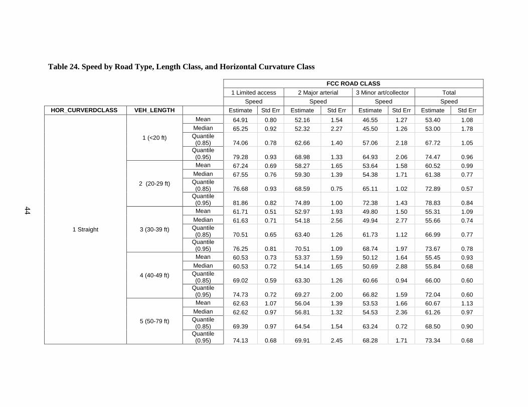
44
Table 24. Speed by Road Type, Length Class, and Horizontal Curvature Class
FCC ROAD CLASS 1 Limited access 2 Major arterial 3 Minor art/collector Total Speed Speed Speed Speed HOR_CURVERDCLASS VEH_LENGTH Estimate Std Err Estimate Std Err Estimate Std Err Estimate Std Err
1 Straight
1 (<20 ft)
Mean 64.91 0.80 52.16 1.54 46.55 1.27 53.40 1.08 Median 65.25 0.92 52.32 2.27 45.50 1.26 53.00 1.78 Quantile
(0.85) 74.06 0.78 62.66 1.40 57.06 2.18 67.72 1.05 Quantile
(0.95) 79.28 0.93 68.98 1.33 64.93 2.06 74.47 0.96
2 (20-29 ft)
Mean 67.24 0.69 58.27 1.65 53.64 1.58 60.52 0.99 Median 67.55 0.76 59.30 1.39 54.38 1.71 61.38 0.77 Quantile
(0.85) 76.68 0.93 68.59 0.75 65.11 1.02 72.89 0.57 Quantile
(0.95) 81.86 0.82 74.89 1.00 72.38 1.43 78.83 0.84
3 (30-39 ft)
Mean 61.71 0.51 52.97 1.93 49.80 1.50 55.31 1.09 Median 61.63 0.71 54.18 2.56 49.94 2.77 55.66 0.74 Quantile
(0.85) 70.51 0.65 63.40 1.26 61.73 1.12 66.99 0.77 Quantile
(0.95) 76.25 0.81 70.51 1.09 68.74 1.97 73.67 0.78
4 (40-49 ft)
Mean 60.53 0.73 53.37 1.59 50.12 1.64 55.45 0.93 Median 60.53 0.72 54.14 1.65 50.69 2.88 55.84 0.68 Quantile
(0.85) 69.02 0.59 63.30 1.26 60.66 0.94 66.00 0.60 Quantile
(0.95) 74.73 0.72 69.27 2.00 66.82 1.59 72.04 0.60
5 (50-79 ft)
Mean 62.63 1.07 56.04 1.39 53.53 1.66 60.67 1.13 Median 62.62 0.97 56.81 1.32 54.53 2.36 61.26 0.97 Quantile
(0.85) 69.39 0.97 64.54 1.54 63.24 0.72 68.50 0.90 Quantile
(0.95) 74.13 0.68 69.91 2.45 68.28 1.71 73.34 0.68

45
FCC ROAD CLASS 1 Limited access 2 Major arterial 3 Minor art/collector Total Speed Speed Speed Speed HOR_CURVERDCLASS VEH_LENGTH Estimate Std Err Estimate Std Err Estimate Std Err Estimate Std Err
6 (80-100 ft)
Mean 66.81 1.53 61.26 1.59 57.79 2.34 65.70 1.32 Median 66.45 1.15 62.65 1.04 58.66 4.17 65.98 0.93 Quantile
(0.85) 74.38 1.60 69.42 3.90 68.84 3.74 73.77 1.58 Quantile
(0.95) 80.23 2.52 73.99 4.62 72.81 3.03 79.55 1.99
Total
Mean 64.89 0.68 53.32 1.69 47.63 1.41 55.03 1.22 Median 65.08 0.73 53.92 2.38 46.59 1.56 55.35 1.54 Quantile
(0.85) 74.00 0.70 64.19 1.38 58.93 1.93 68.78 0.82 Quantile
(0.95) 79.35 0.81 70.39 1.18 66.56 1.85 75.27 0.79
2 Moderate
1 (< 20 ft)
Mean 60.60 4.76 57.94 2.21 40.39 1.74 45.95 2.31 Median 60.31 5.32 57.67 2.63 38.83 1.12 43.02 3.34 Quantile
(0.85) 70.16 3.74 66.72 3.94 50.28 4.49 60.89 2.75 Quantile
(0.95) 75.47 3.47 72.10 3.64 59.00 3.63 68.52 2.20
2 (20-29 ft)
Mean 64.40 3.79 63.10 3.20 45.22 3.14 54.23 3.20 Median 64.44 3.75 62.80 3.22 45.42 3.84 56.30 3.52 Quantile
(0.85) 74.06 2.86 72.43 4.66 58.30 2.95 68.76 2.52 Quantile
(0.95) 79.36 2.79 77.46 4.13 64.38 2.39 75.48 1.82
3 (30-39 ft)
Mean 56.93 4.02 58.09 2.92 44.31 2.79 50.03 2.43 Median 56.45 4.71 57.03 2.44 42.89 4.95 51.49 2.64 Quantile
(0.85) 66.14 2.74 67.08 5.16 56.84 3.30 62.85 1.97 Quantile
(0.95) 71.34 2.62 72.27 3.34 63.09 2.72 68.96 1.62
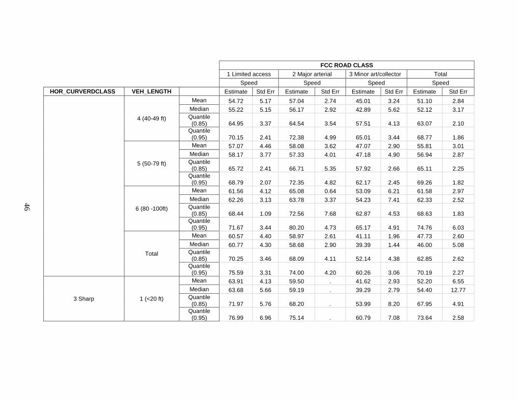
46
FCC ROAD CLASS 1 Limited access 2 Major arterial 3 Minor art/collector Total Speed Speed Speed Speed HOR_CURVERDCLASS VEH_LENGTH Estimate Std Err Estimate Std Err Estimate Std Err Estimate Std Err
4 (40-49 ft)
Mean 54.72 5.17 57.04 2.74 45.01 3.24 51.10 2.84 Median 55.22 5.15 56.17 2.92 42.89 5.62 52.12 3.17 Quantile
(0.85) 64.95 3.37 64.54 3.54 57.51 4.13 63.07 2.10 Quantile
(0.95) 70.15 2.41 72.38 4.99 65.01 3.44 68.77 1.86
5 (50-79 ft)
Mean 57.07 4.46 58.08 3.62 47.07 2.90 55.81 3.01 Median 58.17 3.77 57.33 4.01 47.18 4.90 56.94 2.87 Quantile
(0.85) 65.72 2.41 66.71 5.35 57.92 2.66 65.11 2.25 Quantile
(0.95) 68.79 2.07 72.35 4.82 62.17 2.45 69.26 1.82
6 (80 -100ft)
Mean 61.56 4.12 65.08 0.64 53.09 6.21 61.58 2.97 Median 62.26 3.13 63.78 3.37 54.23 7.41 62.33 2.52 Quantile
(0.85) 68.44 1.09 72.56 7.68 62.87 4.53 68.63 1.83 Quantile
(0.95) 71.67 3.44 80.20 4.73 65.17 4.91 74.76 6.03
Total
Mean 60.57 4.40 58.97 2.61 41.11 1.96 47.73 2.60 Median 60.77 4.30 58.68 2.90 39.39 1.44 46.00 5.08 Quantile
(0.85) 70.25 3.46 68.09 4.11 52.14 4.38 62.85 2.62 Quantile
(0.95) 75.59 3.31 74.00 4.20 60.26 3.06 70.19 2.27
3 Sharp 1 (<20 ft)
Mean 63.91 4.13 59.50 . 41.62 2.93 52.20 6.55 Median 63.68 5.66 59.19 . 39.29 2.79 54.40 12.77 Quantile
(0.85) 71.97 5.76 68.20 . 53.99 8.20 67.95 4.91 Quantile
(0.95) 76.99 6.96 75.14 . 60.79 7.08 73.64 2.58

47
FCC ROAD CLASS 1 Limited access 2 Major arterial 3 Minor art/collector Total Speed Speed Speed Speed HOR_CURVERDCLASS VEH_LENGTH Estimate Std Err Estimate Std Err Estimate Std Err Estimate Std Err
2 (20-29 ft)
Mean 65.76 1.32 62.40 . 45.83 3.34 58.36 8.11 Median 65.47 0.43 62.36 . 45.27 5.17 60.61 10.10 Quantile
(0.85) 73.01 3.58 72.88 . 57.60 2.95 70.60 6.49 Quantile
(0.95) 79.11 7.08 78.62 . 63.23 3.13 76.98 4.16
3 (30-39 ft)
Mean 61.97 1.20 56.29 . 46.34 4.78 54.46 3.92 Median 61.40 1.61 57.90 . 48.97 10.20 57.00 2.91 Quantile
(0.85) 69.49 0.62 68.99 . 58.00 3.29 66.05 3.24 Quantile
(0.95) 75.14 1.15 73.09 . 61.90 2.24 71.98 2.25
4 (40-49 ft)
Mean 60.34 0.56 53.43 . 43.80 3.43 55.00 5.66 Median 59.98 0.91 50.82 . 41.14 6.25 57.00 6.77 Quantile
(0.85) 67.58 1.28 63.26 . 55.55 4.02 65.32 3.25 Quantile
(0.95) 72.50 1.26 78.78 . 63.00 2.84 71.33 1.79
5 (50-79 ft)
Mean 59.14 1.76 53.74 . 45.12 2.08 57.17 2.69 Median 58.58 1.45 54.52 . 44.60 3.31 57.74 0.97 Quantile
(0.85) 65.31 1.55 65.94 . 56.99 4.99 64.99 0.43 Quantile
(0.95) 69.57 2.22 70.40 . 61.93 1.96 69.47 0.55
6 (80-100 ft)
Mean 61.36 9.08 59.49 . 36.18 2.35 59.65 6.13 Median 60.96 8.09 59.49 . 35.43 3.24 60.17 0.84 Quantile
(0.85) 66.41 5.73 59.49 . 38.57 2.48 66.34 3.22 Quantile
(0.95) 71.98 1.87 59.49 . 40.22 3.04 71.48 2.79

48
FCC ROAD CLASS 1 Limited access 2 Major arterial 3 Minor art/collector Total Speed Speed Speed Speed HOR_CURVERDCLASS VEH_LENGTH Estimate Std Err Estimate Std Err Estimate Std Err Estimate Std Err
Total
Mean 63.87 3.61 59.23 . 42.04 2.93 53.04 6.69 Median 63.53 4.98 59.34 . 39.69 3.17 55.62 12.59 Quantile
(0.85) 71.95 4.87 69.01 . 54.38 7.25 68.20 4.96 Quantile
(0.95) 77.25 6.36 75.72 . 60.98 5.51 73.95 2.24
Total
1 (<20 ft)
Mean 64.72 0.86 52.45 1.56 45.80 1.29 52.88 1.07 Median 65.08 0.93 52.75 2.15 44.74 1.23 52.63 1.72 Quantile
(0.85) 73.84 0.91 63.00 1.52 56.53 2.09 67.44 1.02 Quantile
(0.95) 79.04 0.92 69.18 1.29 64.30 2.19 74.21 0.89
2 (20-29 ft)
Mean 67.08 0.73 58.59 1.69 52.75 1.71 60.10 1.08 Median 67.33 0.88 59.54 1.32 53.82 2.10 61.03 0.87 Quantile
(0.85) 76.41 0.87 68.91 0.75 64.48 1.16 72.67 0.69 Quantile
(0.95) 81.80 0.96 75.22 0.90 71.87 1.42 78.62 0.65
3 (30-39 ft)
Mean 61.53 0.60 53.29 1.96 49.18 1.56 54.95 1.12 Median 61.38 0.75 54.51 2.43 49.30 2.84 55.50 0.68 Quantile
(0.85) 70.29 0.65 63.75 1.46 61.09 0.98 66.79 0.77 Quantile
(0.95) 76.17 0.45 70.53 0.98 68.11 1.82 73.28 0.89
4 (40-49 ft)
Mean 60.24 0.88 53.59 1.59 49.60 1.77 55.17 1.02 Median 60.32 0.67 54.34 1.65 50.03 2.92 55.61 0.76 Quantile
(0.85) 68.89 0.66 63.60 1.08 60.43 1.15 65.95 0.46 Quantile
(0.95) 74.41 0.83 69.60 1.88 66.70 1.35 71.90 0.68

49
FCC ROAD CLASS 1 Limited access 2 Major arterial 3 Minor art/collector Total Speed Speed Speed Speed HOR_CURVERDCLASS VEH_LENGTH Estimate Std Err Estimate Std Err Estimate Std Err Estimate Std Err
5 (50-79 ft)
Mean 62.36 1.18 56.15 1.44 53.08 1.72 60.40 1.21 Median 62.48 1.18 56.86 1.45 54.16 2.51 61.03 1.00 Quantile
(0.85) 69.29 1.02 64.64 1.38 63.05 0.55 68.25 0.88 Quantile
(0.95) 74.12 0.93 70.04 2.24 68.18 1.29 73.21 0.75
6 (80-100 ft)
Mean 66.54 1.58 61.71 1.41 57.18 2.78 65.43 1.39 Median 66.41 1.03 62.93 1.12 58.56 4.87 65.76 0.94 Quantile
(0.85) 74.18 1.82 70.23 4.15 68.56 3.30 73.68 1.53 Quantile
(0.95) 80.05 2.56 75.03 4.42 72.72 2.47 79.53 1.97
Total
Mean 64.69 0.76 53.62 1.71 46.85 1.43 54.51 1.23 Median 64.86 0.79 54.10 2.22 45.85 1.62 55.02 1.66 Quantile
(0.85) 73.77 0.73 64.46 1.38 58.30 2.09 68.48 0.92 Quantile
(0.95) 79.20 0.79 70.64 1.28 65.95 1.69 75.06 0.77
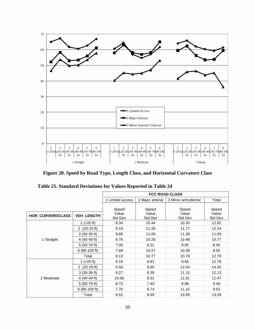
50
Figure 20. Speed by Road Type, Length Class, and Horizontal Curvature Class
Table 25. Standard Deviations for Values Reported in Table 24
FCC ROAD CLASS 1 Limited access 2 Major arterial 3 Minor art/collector Total
Speed Value
Std Dev
Speed Value
Std Dev
Speed Value
Std Dev
Speed Value
Std Dev
HOR_CURVERDCLASS VEH_LENGTH
1 Straight
1 (<20 ft) 9.34 10.44 10.30 12.82 2 (20-29 ft) 9.19 11.26 11.77 12.24 3 (30-39 ft) 8.89 11.00 11.39 11.69 4 (40-49 ft) 8.76 10.28 10.48 10.77 5 (50-79 ft) 7.00 9.21 9.95 8.45
6 (80-100 ft) 7.68 10.07 10.38 8.55 Total 9.13 10.77 10.79 12.79
2 Moderate
1 (<20 ft) 9.19 8.81 9.56 12.78 2 (20-29 ft) 9.50 8.60 12.04 14.20 3 (30-39 ft) 9.27 8.39 11.15 12.13 4 (40-49 ft) 10.06 8.51 11.01 11.47 5 (50-79 ft) 8.72 7.93 9.98 9.49
6 (80-100 ft) 7.76 8.74 11.15 9.02 Total 9.52 8.95 10.06 13.29
0
10
20
30
40
50
60
70
1 (<20 ft)
2 (20-29
ft)
3 (30-39
ft)
4 (40-49
ft)
5 (50-79
ft)
6 (80-100
ft)
1 (<20 ft)
2 (20-29
ft)
3 (30-39
ft)
4 (40-49
ft)
5 (50-79
ft)
6 (80-100
ft)
1 (<20 ft)
2 (20-29
ft)
3 (30-39
ft)
4 (40-49
ft)
5 (50-79
ft)
6 (80-100
ft)
1 Straight 2 Moderate 3 Sharp
1 Limited Access
2 Major Arterial
3 Minor Arterial/ Collector

51
FCC ROAD CLASS 1 Limited access 2 Major arterial 3 Minor art/collector Total
Speed Value
Std Dev
Speed Value
Std Dev
Speed Value
Std Dev
Speed Value
Std Dev
HOR_CURVERDCLASS VEH_LENGTH
3 Sharp
1 (<20 ft) 8.48 8.80 9.94 14.43 2 (20-29 ft) 7.67 10.43 11.06 13.20 3 (30-39 ft) 7.50 12.18 11.93 12.60 4 (40-49 ft) 7.03 12.06 11.17 11.55 5 (50-79 ft) 6.10 11.45 11.00 8.61
6 (80-100 ft) 5.49 . 3.28 8.09 Total 8.36 9.93 10.15 14.27
Total
1 (<20 ft) 9.32 10.45 10.41 13.01 2 (20-29 ft) 9.18 11.18 12.06 12.48 3 (30-39 ft) 8.91 10.95 11.51 11.82 4 (40-49 ft) 8.87 10.23 10.66 10.88 5 (50-79 ft) 7.16 9.17 10.11 8.57
6 (80-100 ft) 7.75 9.97 10.71 8.64 Total 9.15 10.76 10.91 12.99
5.11 Vertical Curvature and Vehicle Length Table 26 and Table 27 present the relationship among vehicle length and hilliness (steepness of gradient) as a function of roadway class. The highest speeds were for passenger vehicles, light trucks, and the biggest trucks on flat freeway segments, while the lowest were for the medium and large trucks on minor arterials with steep gradients. For each vehicle type, there was little difference in speeds between moderate and steep grades on freeways. Notable anomalies were found for big trucks, especially for moderate gradient on minor arterials, where speeds were unexpectedly high, although the relatively high standard errors of the estimates indicate a high variation in speeds and/or sample in those cells. Figure 21 provides a graphic view of the statistics from Table 26.

52
Table 26. Speed by Road Type, Length Class, and Vertical Curvature Class
FCC ROAD CLASS
1 Limited access 2 Major arterial 3 Minor art/collector Total Speed Speed Speed Speed VER_CURVERDCLASS VEH_LENGTH Estimate Std Err Estimate Std Err Estimate Std Err Estimate Std Err
1 Flat
1 (<20ft)
Mean 64.80 0.90 52.37 1.54 45.98 1.26 53.08 1.06 Median 65.15 0.96 52.75 2.13 44.98 1.24 52.78 1.70
Quantile (0.85) 74.00 0.80 63.00 1.47 56.82 2.09 67.60 1.00 Quantile (0.95) 79.24 0.95 69.05 1.11 64.47 2.21 74.38 0.97
2 (20-29 ft)
Mean 67.13 0.74 58.55 1.72 52.81 1.58 60.28 1.07 Median 67.44 0.86 59.54 1.37 53.87 1.89 61.13 0.97
Quantile (0.85) 76.47 0.85 68.91 0.77 64.51 1.14 72.85 0.65 Quantile (0.95) 81.84 0.87 75.15 0.86 72.04 1.57 78.71 0.85
3 (30-39 ft)
Mean 61.53 0.62 53.34 1.92 49.33 1.47 55.11 1.10 Median 61.39 0.79 54.59 2.45 49.62 2.72 55.55 0.73
Quantile (0.85) 70.41 0.65 63.77 1.44 61.11 1.04 66.83 0.75 Quantile (0.95) 76.18 0.51 70.51 0.75 68.19 1.83 73.49 0.86
4 (40-49 ft)
Mean 60.23 0.91 53.62 1.49 49.64 1.64 55.28 0.99 Median 60.33 0.71 54.35 1.55 50.09 2.73 55.62 0.75
Quantile (0.85) 68.91 0.66 63.48 1.03 60.15 1.26 65.98 0.48 Quantile (0.95) 74.54 0.89 69.31 1.46 66.70 1.55 72.00 0.60
5 (50-79 ft)
Mean 62.40 1.18 56.07 1.49 52.80 1.42 60.48 1.22 Median 62.58 1.17 56.78 1.53 53.99 2.05 61.07 0.99
Quantile (0.85) 69.32 1.02 64.54 1.08 62.93 1.28 68.38 0.87 Quantile (0.95) 74.12 0.91 69.84 1.88 68.26 1.74 73.21 0.73
6 (80-100 ft)
Mean 66.61 1.57 61.63 1.39 56.11 2.19 65.47 1.39 Median 66.42 1.07 62.79 1.24 56.55 3.39 65.83 0.99
Quantile (0.85) 74.23 1.80 69.59 3.52 66.27 4.76 73.72 1.57 Quantile (0.95) 80.12 2.50 75.10 5.34 72.84 2.49 79.55 1.94
Total
Mean 64.76 0.78 53.57 1.71 46.99 1.37 54.71 1.22 Median 64.98 0.88 54.04 2.19 45.97 1.47 55.22 1.51
Quantile (0.85) 73.93 0.73 64.46 1.37 58.37 1.93 68.69 0.86 Quantile (0.95) 79.33 0.86 70.56 1.12 66.00 1.86 75.23 0.79

53
FCC ROAD CLASS
1 Limited access 2 Major arterial 3 Minor art/collector Total Speed Speed Speed Speed VER_CURVERDCLASS VEH_LENGTH Estimate Std Err Estimate Std Err Estimate Std Err Estimate Std Err
2 Moderate
1 (<20 ft)
Mean 62.80 . 54.56 . 43.95 3.42 50.30 5.04 Median 62.49 . 54.93 . 41.68 2.83 50.29 8.68
Quantile (0.85) 69.89 . 59.22 . 55.84 7.40 64.09 5.86 Quantile (0.95) 74.33 . 61.85 . 62.76 6.03 70.02 6.23
2 (20-29 ft)
Mean 65.65 . 58.22 . 53.49 6.07 57.44 3.46 Median 65.45 . 58.93 . 55.22 7.36 59.36 3.48
Quantile (0.85) 72.84 . 62.79 . 65.13 5.81 68.33 3.16 Quantile (0.95) 78.91 . 65.56 . 69.94 5.05 73.65 4.12
3 (30-39 ft)
Mean 61.52 . 56.78 . 48.34 4.95 52.98 3.64 Median 60.80 . 57.15 . 48.39 6.05 54.91 4.57
Quantile (0.85) 69.01 . 60.80 . 61.64 5.67 64.99 2.82 Quantile (0.95) 75.32 . 62.33 . 66.45 5.15 70.00 3.04
4 (40-49 ft)
Mean 60.44 . 55.78 . 50.15 6.43 53.84 3.32 Median 60.15 . 56.19 . 50.06 7.52 56.11 4.53
Quantile (0.85) 67.43 . 59.76 . 63.28 7.72 64.10 0.92 Quantile (0.95) 72.09 . 62.03 . 66.23 2.67 68.99 2.81
5 (50-79 ft)
Mean 58.68 . 53.55 . 56.21 10.31 57.17 1.87 Median 58.06 . 53.99 . 59.12 12.74 58.50 1.99
Quantile (0.85) 64.69 . 59.84 . 64.43 8.60 64.47 0.94 Quantile (0.95) 69.05 . 60.29 . 67.39 6.28 68.17 0.80
6 (80-100 ft)
Mean 60.86 . . . 65.63 11.39 62.87 3.16 Median 60.68 . . . 64.74 7.45 62.90 2.87
Quantile (0.85) 65.68 . . . 69.64 10.27 68.94 3.87 Quantile (0.95) 69.30 . . . 71.47 11.45 72.19 2.02
Total
Mean 62.99 . 55.03 . 45.86 4.49 51.64 4.73 Median 62.69 . 55.39 . 43.49 4.52 52.78 8.17
Quantile (0.85) 70.39 . 59.72 . 59.30 8.31 64.98 4.67 Quantile (0.95) 75.07 . 62.71 . 65.13 6.22 70.50 4.89

54
FCC ROAD CLASS
1 Limited access 2 Major arterial 3 Minor art/collector Total Speed Speed Speed Speed VER_CURVERDCLASS VEH_LENGTH Estimate Std Err Estimate Std Err Estimate Std Err Estimate Std Err
3 Steep
1 (<20 ft)
Mean 60.32 . 55.39 13.54 41.24 3.16 45.26 4.19 Median 60.33 . 55.29 14.30 41.52 3.92 43.02 1.94
Quantile (0.85) 66.68 . 70.39 20.81 47.81 2.45 56.32 11.99 Quantile (0.95) 71.10 . 78.67 22.71 51.68 2.55 69.09 15.15
2 (20-29 ft)
Mean 64.30 . 62.35 12.73 43.79 6.91 49.96 6.05 Median 63.57 . 62.66 14.63 44.40 10.47 48.50 5.46
Quantile (0.85) 71.41 . 75.91 11.95 54.77 5.13 65.15 10.38 Quantile (0.95) 76.82 . 83.52 12.10 60.59 4.97 75.86 11.07
3 (30-39 ft)
Mean 59.59 . 49.71 13.85 39.44 5.62 44.82 5.30 Median 58.60 . 42.91 15.91 37.44 6.72 41.06 3.39
Quantile (0.85) 66.68 . 64.04 20.52 48.55 5.19 60.57 13.01 Quantile (0.95) 76.44 . 73.35 25.52 60.86 10.84 69.95 10.80
4 (40-49 ft)
Mean 57.10 . 52.38 13.35 40.46 4.50 49.21 8.69 Median 57.26 . 51.65 13.70 39.99 6.65 45.08 10.81
Quantile (0.85) 63.46 . 67.15 21.82 47.33 2.65 65.10 17.07 Quantile (0.95) 67.34 . 73.86 23.61 54.07 6.04 72.67 17.51
5 (50-79 ft)
Mean 58.25 . 60.74 17.22 39.84 3.29 57.91 14.87 Median 58.41 . 59.95 17.17 39.19 2.72 58.80 15.98
Quantile (0.85) 65.10 . 73.21 26.01 48.60 2.93 72.97 21.92 Quantile (0.95) 69.52 . 77.28 23.51 52.90 3.24 76.62 16.25
6 (80-100 ft)
Mean 63.04 . 74.01 . 40.44 . 67.19 20.43 Median 65.11 . 74.01 . 40.44 . 71.11 27.43
Quantile (0.85) 67.39 . 74.01 . 40.44 . 73.14 13.35 Quantile (0.95) 68.82 . 74.01 . 40.44 . 73.72 6.37
Total
Mean 61.01 . 56.25 13.67 41.47 3.56 46.08 4.71 Median 60.89 . 57.29 15.10 41.58 4.46 43.49 2.29
Quantile (0.85) 67.61 . 71.89 21.25 48.13 2.33 59.23 11.94 Quantile (0.95) 72.57 . 78.86 20.68 52.92 3.06 70.92 15.01
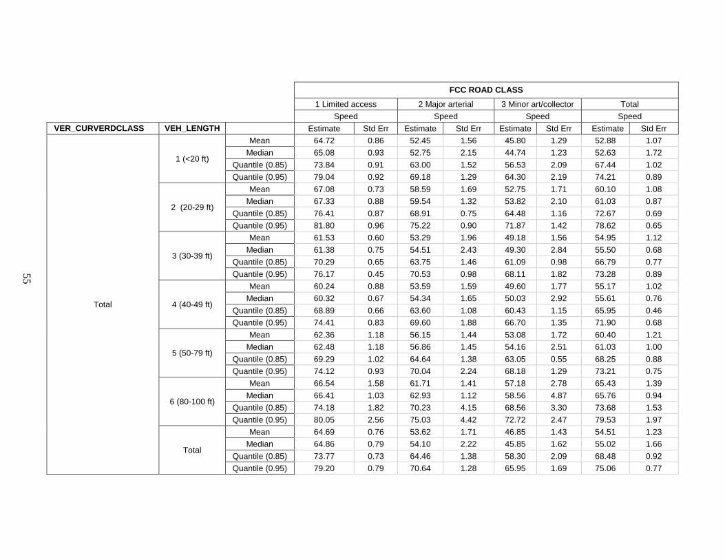
55
FCC ROAD CLASS
1 Limited access 2 Major arterial 3 Minor art/collector Total Speed Speed Speed Speed VER_CURVERDCLASS VEH_LENGTH Estimate Std Err Estimate Std Err Estimate Std Err Estimate Std Err
Total
1 (<20 ft)
Mean 64.72 0.86 52.45 1.56 45.80 1.29 52.88 1.07 Median 65.08 0.93 52.75 2.15 44.74 1.23 52.63 1.72
Quantile (0.85) 73.84 0.91 63.00 1.52 56.53 2.09 67.44 1.02 Quantile (0.95) 79.04 0.92 69.18 1.29 64.30 2.19 74.21 0.89
2 (20-29 ft)
Mean 67.08 0.73 58.59 1.69 52.75 1.71 60.10 1.08 Median 67.33 0.88 59.54 1.32 53.82 2.10 61.03 0.87
Quantile (0.85) 76.41 0.87 68.91 0.75 64.48 1.16 72.67 0.69 Quantile (0.95) 81.80 0.96 75.22 0.90 71.87 1.42 78.62 0.65
3 (30-39 ft)
Mean 61.53 0.60 53.29 1.96 49.18 1.56 54.95 1.12 Median 61.38 0.75 54.51 2.43 49.30 2.84 55.50 0.68
Quantile (0.85) 70.29 0.65 63.75 1.46 61.09 0.98 66.79 0.77 Quantile (0.95) 76.17 0.45 70.53 0.98 68.11 1.82 73.28 0.89
4 (40-49 ft)
Mean 60.24 0.88 53.59 1.59 49.60 1.77 55.17 1.02 Median 60.32 0.67 54.34 1.65 50.03 2.92 55.61 0.76
Quantile (0.85) 68.89 0.66 63.60 1.08 60.43 1.15 65.95 0.46 Quantile (0.95) 74.41 0.83 69.60 1.88 66.70 1.35 71.90 0.68
5 (50-79 ft)
Mean 62.36 1.18 56.15 1.44 53.08 1.72 60.40 1.21 Median 62.48 1.18 56.86 1.45 54.16 2.51 61.03 1.00
Quantile (0.85) 69.29 1.02 64.64 1.38 63.05 0.55 68.25 0.88 Quantile (0.95) 74.12 0.93 70.04 2.24 68.18 1.29 73.21 0.75
6 (80-100 ft)
Mean 66.54 1.58 61.71 1.41 57.18 2.78 65.43 1.39 Median 66.41 1.03 62.93 1.12 58.56 4.87 65.76 0.94
Quantile (0.85) 74.18 1.82 70.23 4.15 68.56 3.30 73.68 1.53 Quantile (0.95) 80.05 2.56 75.03 4.42 72.72 2.47 79.53 1.97
Total
Mean 64.69 0.76 53.62 1.71 46.85 1.43 54.51 1.23 Median 64.86 0.79 54.10 2.22 45.85 1.62 55.02 1.66
Quantile (0.85) 73.77 0.73 64.46 1.38 58.30 2.09 68.48 0.92 Quantile (0.95) 79.20 0.79 70.64 1.28 65.95 1.69 75.06 0.77
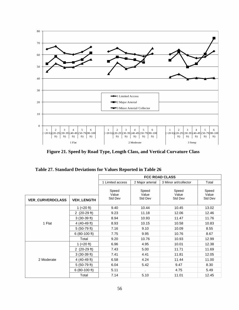
56
Figure 21. Speed by Road Type, Length Class, and Vertical Curvature Class
Table 27. Standard Deviations for Values Reported in Table 26
FCC ROAD CLASS 1 Limited access 2 Major arterial 3 Minor art/collector Total
Speed Value
Std Dev
Speed Value
Std Dev
Speed Value
Std Dev
Speed Value
Std Dev
VER_CURVERDCLASS VEH_LENGTH
1 Flat
1 (<20 ft) 9.40 10.44 10.45 13.02 2 (20-29 ft) 9.23 11.18 12.06 12.46 3 (30-39 ft) 8.94 10.93 11.47 11.76 4 (40-49 ft) 8.93 10.15 10.58 10.83 5 (50-79 ft) 7.16 9.10 10.09 8.55
6 (80-100 ft) 7.75 9.95 10.76 8.67 Total 9.20 10.76 10.93 12.99
2 Moderate
1 (<20 ft) 6.96 4.95 10.01 12.38 2 (20-29 ft) 7.43 5.00 11.71 11.69 3 (30-39 ft) 7.41 4.41 11.81 12.05 4 (40-49 ft) 6.58 4.24 11.44 11.00 5 (50-79 ft) 6.04 5.42 9.47 8.30
6 (80-100 ft) 5.11 . 4.75 5.49 Total 7.14 5.10 11.01 12.45
0
10
20
30
40
50
60
70
80
1 (<20 ft)
2 (20-29
ft)
3 (30-39
ft)
4 (40-49
ft)
5 (50-79
ft)
6 (80-100
ft)
1 (<20 ft)
2 (20-29
ft)
3 (30-39
ft)
4 (40-49
ft)
5 (50-79
ft)
6 (80-100
ft)
1 (<20 ft)
2 (20-29
ft)
3 (30-39
ft)
4 (40-49
ft)
5 (50-79
ft)
6 (80-100
ft)
1 Flat 2 Moderate 3 Steep
1 Limited Access
2 Major Arterial
3 Minor Arterial/ Collector

57
FCC ROAD CLASS 1 Limited access 2 Major arterial 3 Minor art/collector Total
Speed Value
Std Dev
Speed Value
Std Dev
Speed Value
Std Dev
Speed Value
Std Dev
VER_CURVERDCLASS VEH_LENGTH
3 Steep
1 (<20 ft) 6.58 13.87 6.57 11.17 2 (20-29 ft) 7.08 14.09 10.31 14.49 3 (30-39 ft) 7.91 12.69 9.69 12.49 4 (40-49 ft) 7.16 12.93 8.46 12.98 5 (50-79 ft) 7.02 11.78 7.98 13.35
6 (80-100 ft) 7.34 . . 13.21 Total 6.92 13.98 7.14 11.89
Total
1 (<20 ft) 9.32 10.45 10.41 13.01 2 (20-29 ft) 9.18 11.18 12.06 12.48 3 (30-39 ft) 8.91 10.95 11.51 11.82 4 (40-49 ft) 8.87 10.23 10.66 10.88 5 (50-79 ft) 7.16 9.17 10.11 8.57
6 (80-100 ft) 7.75 9.97 10.71 8.64 Total 9.15 10.76 10.91 12.99
5.12 Horizontal Curvature and Light Condition Table 28 and Table 29 present the relationship among roadway curviness and light condition as a function of FCC roadway class. Here the results show little impact from the light condition and relatively similar patterns based on horizontal curvature within each roadway class. Nighttime speeds of the largest trucks were similar to their daytime speeds on freeways, but were about 1 to 2 mph faster than their daytime speeds on arterials and collector roads. The daylight means are slightly higher than nighttime means, but the difference is not statistically significant. Figure 22 provides a graphic view of the statistics from Table 28.
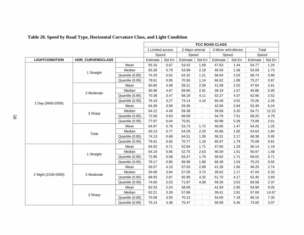
58
Table 28. Speed by Road Type, Horizontal Curvature Class, and Light Condition
FCC ROAD CLASS 1 Limited access 2 Major arterial 3 Minor art/collector Total Speed Speed Speed Speed
LIGHTCONDITION HOR_CURVERDCLASS Estimate Std Err Estimate Std Err Estimate Std Err Estimate Std Err
1 Day (0600-2059)
1 Straight
Mean 65.16 0.67 53.42 1.69 47.63 1.44 54.77 1.24 Median 65.28 0.79 53.99 2.18 46.59 1.58 55.09 1.73
Quantile (0.85) 74.25 0.62 64.32 1.21 58.94 2.03 68.74 0.89 Quantile (0.95) 79.61 0.95 70.50 1.14 66.62 1.89 75.27 0.87
2 Moderate
Mean 60.85 4.48 59.21 2.59 41.08 2.02 47.64 2.61 Median 60.96 4.67 58.90 2.91 39.19 1.57 45.86 5.00
Quantile (0.85) 70.38 3.47 68.18 4.11 52.27 4.37 62.96 2.52 Quantile (0.95) 76.19 3.27 74.14 4.10 60.48 3.02 70.26 2.26
3 Sharp
Mean 64.39 3.58 59.36 . 42.06 2.94 52.49 6.24 Median 64.12 4.49 59.38 . 39.69 3.20 54.71 12.22
Quantile (0.85) 72.06 5.63 68.99 . 54.79 7.51 68.20 4.79 Quantile (0.95) 77.97 6.04 75.81 . 60.98 5.39 73.99 2.61
Total
Mean 64.97 0.76 53.73 1.72 46.85 1.47 54.25 1.25 Median 65.13 0.77 54.29 2.20 45.86 1.65 54.63 1.84
Quantile (0.85) 74.13 0.68 64.51 1.30 58.31 2.17 68.38 0.95 Quantile (0.95) 79.41 0.92 70.77 1.19 65.97 1.79 75.08 0.81
2 Night (2100-0559)
1 Straight
Mean 64.02 0.71 52.84 1.71 47.60 1.29 56.14 1.19 Median 64.19 0.66 52.75 2.63 46.59 1.51 56.97 1.48
Quantile (0.85) 72.85 0.58 63.47 1.79 58.92 1.71 69.02 0.71 Quantile (0.95) 78.17 0.85 69.99 1.89 66.39 1.54 75.23 0.55
2 Moderate
Mean 59.57 4.10 57.63 2.89 41.28 1.66 48.20 2.74 Median 59.68 3.84 57.05 3.72 39.62 1.17 47.04 5.33
Quantile (0.85) 68.93 2.87 65.99 4.32 51.70 4.17 62.45 2.69 Quantile (0.95) 74.60 2.53 71.87 4.08 59.26 3.02 69.58 2.37
3 Sharp
Mean 62.53 2.24 58.09 . 41.93 2.95 54.99 9.05 Median 62.21 3.39 57.88 . 39.41 2.81 57.69 14.67
Quantile (0.85) 70.08 3.55 70.13 . 54.00 7.18 68.10 7.30 Quantile (0.95) 75.14 4.38 75.47 . 59.99 5.46 73.00 3.07

59
FCC ROAD CLASS 1 Limited access 2 Major arterial 3 Minor art/collector Total Speed Speed Speed Speed
LIGHTCONDITION HOR_CURVERDCLASS Estimate Std Err Estimate Std Err Estimate Std Err Estimate Std Err
Total
Mean 63.80 0.75 53.06 1.70 46.81 1.27 55.65 1.18 Median 63.90 0.73 53.00 2.52 45.69 1.45 56.46 1.49
Quantile (0.85) 72.67 0.76 63.68 1.86 58.25 1.86 68.78 0.79 Quantile (0.95) 77.93 0.70 70.14 1.90 65.76 1.32 75.00 0.69
Total
1 Straight
Mean 64.89 0.68 53.32 1.69 47.63 1.41 55.03 1.22 Median 65.08 0.73 53.92 2.38 46.59 1.56 55.35 1.54
Quantile (0.85) 74.00 0.70 64.19 1.38 58.93 1.93 68.78 0.82 Quantile (0.95) 79.35 0.81 70.39 1.18 66.56 1.85 75.27 0.79
2 Moderate
Mean 60.57 4.40 58.97 2.61 41.11 1.96 47.73 2.60 Median 60.77 4.30 58.68 2.90 39.39 1.44 46.00 5.08
Quantile (0.85) 70.25 3.46 68.09 4.11 52.14 4.38 62.85 2.62 Quantile (0.95) 75.59 3.31 74.00 4.20 60.26 3.06 70.19 2.27
3 Sharp
Mean 63.87 3.61 59.23 . 42.04 2.93 53.04 6.69 Median 63.53 4.98 59.34 . 39.69 3.17 55.62 12.59
Quantile (0.85) 71.95 4.87 69.01 . 54.38 7.25 68.20 4.96 Quantile (0.95) 77.25 6.36 75.72 . 60.98 5.51 73.95 2.24
Total
Mean 64.69 0.76 53.62 1.71 46.85 1.43 54.51 1.23 Median 64.86 0.79 54.10 2.22 45.85 1.62 55.02 1.66
Quantile (0.85) 73.77 0.73 64.46 1.38 58.30 2.09 68.48 0.92 Quantile (0.95) 79.20 0.79 70.64 1.28 65.95 1.69 75.06 0.77

60
Figure 22. Speed by Road Type, Horizontal Curvature Class, and Light Condition
Table 29. Standard Deviations for Values Reported in Table 28
FCC ROAD CLASS 1 Limited access 2 Major arterial 3 Minor art/collector Total
Speed Value
Std Dev
Speed Value
Std Dev
Speed Value
Std Dev
Speed Value
Std Dev
LIGHTCONDITION HOR_CURVERDCLASS
1 Day (0600-2059)
1 Straight 9.20 10.86 10.82 12.88 2 Moderate 9.48 9.07 10.17 13.40
3 Sharp 8.52 9.73 10.18 14.52 Total 9.22 10.85 10.94 13.09
2 Night (2100-0559)
1 Straight 8.85 10.31 10.62 12.32 2 Moderate 9.59 8.15 9.45 12.69
3 Sharp 7.77 11.53 9.99 13.16 Total 8.86 10.28 10.70 12.51
Total
1 Straight 9.13 10.77 10.79 12.79 2 Moderate 9.52 8.95 10.06 13.29
3 Sharp 8.36 9.93 10.15 14.27 Total 9.15 10.76 10.91 12.99
0
10
20
30
40
50
60
70
1 Straight 2 Moderate 3 Sharp 1 Straight 2 Moderate 3 Sharp
1 Day (0600-2059) 2 Night (2100-0559)
1 Limited Access
2 Major Arterial
3 Minor Arterial/ Collector

61
5.13 Vertical Curvature and Light Condition The impact of vertical curvature and light condition within roadway classes is shown in Table 30 and Table 31. Speeds were lower as hilliness increased on FCC-3 roads and FCC-1 roads. The light condition influences on mean speeds are, however, extremely subtle. Patterns of variation in speeds by light and vertical curvature were consistent across FCC classes, with only minimal changes among light conditions for similar FCC/vertical curvature pairings. Figure 23 provides a graphic view of the statistics from Table 30.

62
Table 30. Speed by Road Type, Vertical Curvature Class, and Light Condition
FCC ROAD CLASS 1 Limited access 2 Major arterial 3 Minor art/collector Total Speed Speed Speed Speed
LIGHTCONDITION VER_CURVERDCLASS Estimate Std Err Estimate Std Err Estimate Std Err Estimate Std Err
1 Day (0600-2059)
1 Flat
Mean 65.03 0.79 53.68 1.72 47.00 1.41 54.46 1.24 Median 65.16 0.76 54.25 2.17 45.97 1.49 54.88 1.74
Quantile (0.85) 74.20 0.67 64.51 1.32 58.39 2.00 68.55 0.92 Quantile (0.95) 79.57 0.89 70.64 1.07 66.05 1.98 75.25 0.84
2 Moderate
Mean 63.32 . 55.03 . 45.89 4.43 51.09 4.35 Median 62.96 . 55.35 . 43.51 4.52 51.83 8.07
Quantile (0.85) 70.48 . 59.68 . 59.34 8.14 64.46 4.26 Quantile (0.95) 75.14 . 62.68 . 65.13 5.85 70.39 4.71
3 Steep
Mean 61.10 . 56.36 13.22 41.20 3.45 45.86 4.72 Median 60.97 . 57.69 14.70 41.47 4.55 43.44 2.26
Quantile (0.85) 67.59 . 71.05 20.00 47.92 2.10 59.18 11.82 Quantile (0.95) 72.17 . 77.92 18.59 52.78 2.98 70.06 14.39
Total
Mean 64.97 0.76 53.73 1.72 46.85 1.47 54.25 1.25 Median 65.13 0.77 54.29 2.20 45.86 1.65 54.63 1.84
Quantile (0.85) 74.13 0.68 64.51 1.30 58.31 2.17 68.38 0.95 Quantile (0.95) 79.41 0.92 70.77 1.19 65.97 1.79 75.08 0.81
2 Night (2100-0559)
1 Flat
Mean 63.87 0.79 53.00 1.68 46.95 1.17 55.81 1.17 Median 64.04 0.79 52.98 2.46 45.97 1.37 56.61 1.47
Quantile (0.85) 72.74 0.65 63.48 1.71 58.28 1.67 68.90 0.74 Quantile (0.95) 78.00 0.89 69.92 1.57 65.87 1.28 75.08 0.66
2 Moderate
Mean 62.30 . 55.10 . 45.69 4.83 53.80 6.80 Median 61.91 . 55.84 . 43.32 4.59 55.92 9.96
Quantile (0.85) 69.72 . 60.15 . 59.28 9.32 66.39 5.90 Quantile (0.95) 74.43 . 63.48 . 65.47 7.99 71.35 5.18
3 Steep
Mean 60.65 . 55.81 15.61 42.79 4.03 47.12 4.77 Median 60.38 . 55.16 15.68 42.66 4.64 44.02 2.10
Quantile (0.85) 68.08 . 72.94 24.47 49.29 3.60 59.48 12.62 Quantile (0.95) 73.36 . 79.47 26.51 54.26 4.13 72.04 15.16

63
FCC ROAD CLASS 1 Limited access 2 Major arterial 3 Minor art/collector Total Speed Speed Speed Speed
LIGHTCONDITION VER_CURVERDCLASS Estimate Std Err Estimate Std Err Estimate Std Err Estimate Std Err
Total
Mean 63.80 0.75 53.06 1.70 46.81 1.27 55.65 1.18 Median 63.90 0.73 53.00 2.52 45.69 1.45 56.46 1.49
Quantile (0.85) 72.67 0.76 63.68 1.86 58.25 1.86 68.78 0.79 Quantile (0.95) 77.93 0.70 70.14 1.90 65.76 1.32 75.00 0.69
Total
1 Flat
Mean 64.76 0.78 53.57 1.71 46.99 1.37 54.71 1.22 Median 64.98 0.88 54.04 2.19 45.97 1.47 55.22 1.51
Quantile (0.85) 73.93 0.73 64.46 1.37 58.37 1.93 68.69 0.86 Quantile (0.95) 79.33 0.86 70.56 1.12 66.00 1.86 75.23 0.79
2 Moderate
Mean 62.99 . 55.03 . 45.86 4.49 51.64 4.73 Median 62.69 . 55.39 . 43.49 4.52 52.78 8.17
Quantile (0.85) 70.39 . 59.72 . 59.30 8.31 64.98 4.67 Quantile (0.95) 75.07 . 62.71 . 65.13 6.22 70.50 4.89
3 Steep
Mean 61.01 . 56.25 13.67 41.47 3.56 46.08 4.71 Median 60.89 . 57.29 15.10 41.58 4.46 43.49 2.29
Quantile (0.85) 67.61 . 71.89 21.25 48.13 2.33 59.23 11.94 Quantile (0.95) 72.57 . 78.86 20.68 52.92 3.06 70.92 15.01
Total
Mean 64.69 0.76 53.62 1.71 46.85 1.43 54.51 1.23 Median 64.86 0.79 54.10 2.22 45.85 1.62 55.02 1.66
Quantile (0.85) 73.77 0.73 64.46 1.38 58.30 2.09 68.48 0.92 Quantile (0.95) 79.20 0.79 70.64 1.28 65.95 1.69 75.06 0.77
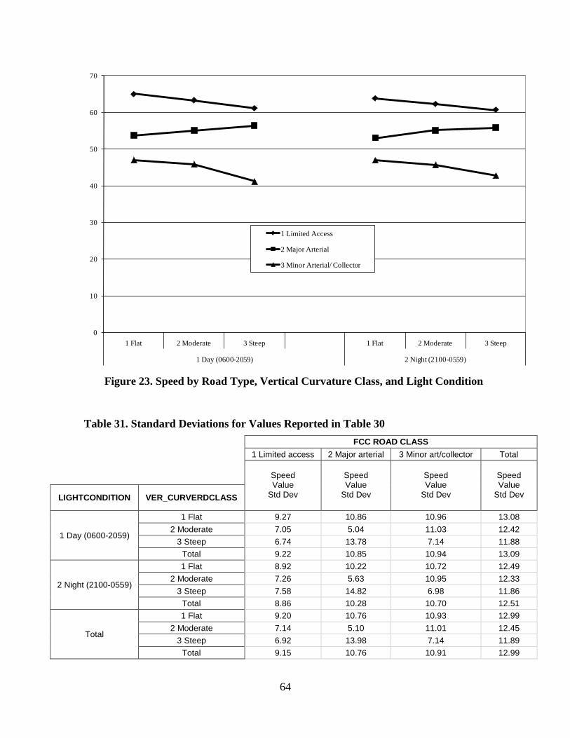
64
Figure 23. Speed by Road Type, Vertical Curvature Class, and Light Condition
Table 31. Standard Deviations for Values Reported in Table 30
FCC ROAD CLASS 1 Limited access 2 Major arterial 3 Minor art/collector Total
Speed Value
Std Dev
Speed Value
Std Dev
Speed Value
Std Dev
Speed Value
Std Dev
LIGHTCONDITION VER_CURVERDCLASS
1 Day (0600-2059)
1 Flat 9.27 10.86 10.96 13.08 2 Moderate 7.05 5.04 11.03 12.42
3 Steep 6.74 13.78 7.14 11.88 Total 9.22 10.85 10.94 13.09
2 Night (2100-0559)
1 Flat 8.92 10.22 10.72 12.49 2 Moderate 7.26 5.63 10.95 12.33
3 Steep 7.58 14.82 6.98 11.86 Total 8.86 10.28 10.70 12.51
Total
1 Flat 9.20 10.76 10.93 12.99 2 Moderate 7.14 5.10 11.01 12.45
3 Steep 6.92 13.98 7.14 11.89 Total 9.15 10.76 10.91 12.99
0
10
20
30
40
50
60
70
1 Flat 2 Moderate 3 Steep 1 Flat 2 Moderate 3 Steep
1 Day (0600-2059) 2 Night (2100-0559)
1 Limited Access
2 Major Arterial
3 Minor Arterial/ Collector

65
5.14 Vehicle Length and Light Condition The influence of vehicle length and light condition on speed for a given roadway class is shown in Table 32 and Table 33. A bi-modal speed distribution by length class within each light condition for each road class is evident. The greatest difference between night and day speeds is associated with the longest vehicle class on major arterial roadways, where speeds at night are approximately 1 to 2 mph higher than daytime speeds. There was also a slight (insignificant) increase associated with the night condition for nearly all of the lengths within each FCC category. Figure 24 provides a graphic view of the statistics from Table 32.

66
Table 32. Speed by Road Type, Length Class, and Light Condition
FCC ROAD CLASS 1 Limited access 2 Major arterial 3 Minor art/collector Total Speed Speed Speed Speed
LIGHTCONDITION VEH_LENGTH Estimate Std Err Estimate Std Err Estimate Std Err Estimate Std Err
1 Day (0600-2059)
1 (<20 ft)
Mean 65.03 0.87 52.60 1.56 45.83 1.32 52.71 1.11 Median 65.45 1.08 53.00 2.21 44.77 1.25 52.27 1.77
Quantile (0.85) 74.14 0.85 63.22 1.44 56.69 2.10 67.35 1.13 Quantile (0.95) 79.36 1.00 69.35 1.26 64.44 2.29 74.23 0.97
2 (20-29 ft)
Mean 67.24 0.73 58.48 1.75 52.49 1.78 59.70 1.15 Median 67.56 0.77 59.54 1.31 53.59 2.26 60.75 1.00
Quantile (0.85) 76.69 0.81 68.91 0.71 64.44 1.16 72.49 0.71 Quantile (0.95) 81.92 0.85 75.21 0.88 71.73 1.57 78.62 0.71
3 (30-39 ft)
Mean 61.57 0.65 53.26 1.94 48.85 1.57 54.47 1.16 Median 61.38 0.84 54.60 2.42 48.99 2.77 55.41 1.03
Quantile (0.85) 70.55 0.68 63.66 1.41 60.76 1.16 66.43 0.86 Quantile (0.95) 76.41 0.69 70.53 0.92 67.48 1.55 73.13 0.64
4 (40-49 ft)
Mean 60.32 0.89 53.65 1.63 49.47 1.82 54.84 1.06 Median 60.42 0.75 54.38 1.66 49.93 2.96 55.41 0.73
Quantile (0.85) 68.99 0.62 63.67 1.13 60.23 1.15 65.72 0.60 Quantile (0.95) 74.61 0.95 69.40 1.74 66.44 1.37 71.69 0.70
5 (50-79 ft)
Mean 62.41 1.14 55.98 1.54 52.85 1.80 60.12 1.24 Median 62.56 1.13 56.64 1.50 54.00 2.77 60.77 0.95
Quantile (0.85) 69.35 0.89 64.55 1.39 63.01 0.71 68.19 0.79 Quantile (0.95) 74.13 0.64 70.00 1.86 68.13 1.38 73.20 0.70
6 (80-100 ft)
Mean 66.72 1.58 61.11 2.02 56.97 2.89 65.36 1.47 Median 66.42 1.09 62.30 1.85 58.61 5.74 65.83 1.12
Quantile (0.85) 74.37 1.68 70.54 3.13 68.76 1.98 73.73 1.43 Quantile (0.95) 80.47 2.51 74.76 8.06 73.42 3.20 80.08 2.35
Total
Mean 64.97 0.76 53.73 1.72 46.85 1.47 54.25 1.25 Median 65.13 0.77 54.29 2.20 45.86 1.65 54.63 1.84
Quantile (0.85) 74.13 0.68 64.51 1.30 58.31 2.17 68.38 0.95 Quantile (0.95) 79.41 0.92 70.77 1.19 65.97 1.79 75.08 0.81

67
FCC ROAD CLASS 1 Limited access 2 Major arterial 3 Minor art/collector Total Speed Speed Speed Speed
LIGHTCONDITION VEH_LENGTH Estimate Std Err Estimate Std Err Estimate Std Err Estimate Std Err
2 Night (2100-0559)
1 (<20 ft)
Mean 63.63 0.82 51.71 1.54 45.63 1.14 53.64 0.99 Median 63.93 0.82 51.47 2.28 44.55 1.23 53.77 1.47
Quantile (0.85) 72.70 0.81 61.94 1.80 56.17 1.89 67.63 0.86 Quantile (0.95) 77.83 0.96 68.38 1.98 63.85 1.75 74.04 0.74
2 (20-29 ft)
Mean 66.56 0.74 59.20 1.40 54.38 1.35 61.97 0.88 Median 66.58 0.93 59.65 1.50 54.82 1.50 62.61 0.68
Quantile (0.85) 75.58 0.88 68.95 0.93 65.56 0.91 73.10 0.58 Quantile (0.95) 80.91 0.80 75.42 1.47 72.38 0.88 78.92 0.87
3 (30-39 ft)
Mean 61.40 0.48 53.50 2.22 51.67 1.62 57.39 1.00 Median 61.38 0.57 54.07 2.97 52.75 2.88 57.97 1.06
Quantile (0.85) 69.79 0.70 63.86 1.72 64.01 1.67 68.06 0.82 Quantile (0.95) 75.69 0.92 70.53 1.85 70.29 3.19 73.78 1.24
4 (40-49 ft)
Mean 59.99 0.88 53.23 1.38 50.55 1.54 56.70 0.88 Median 60.12 0.87 53.56 2.15 51.17 2.89 57.05 0.70
Quantile (0.85) 68.50 0.90 63.27 1.05 61.84 1.58 66.83 0.46 Quantile (0.95) 74.01 0.55 70.05 1.90 67.77 1.84 72.82 0.73
5 (50-79 ft)
Mean 62.25 1.27 56.78 1.12 54.32 1.36 61.15 1.15 Median 62.40 1.28 57.50 1.28 55.22 1.32 61.58 1.11
Quantile (0.85) 69.02 1.32 64.90 1.61 64.00 1.00 68.49 1.02 Quantile (0.95) 73.67 1.25 70.38 2.99 69.05 1.09 73.20 1.00
6 (80-100 ft)
Mean 66.18 1.62 63.32 1.60 58.01 2.25 65.57 1.37 Median 66.31 1.32 63.04 1.88 58.34 1.79 65.69 0.88
Quantile (0.85) 73.73 2.41 67.61 6.76 63.98 4.62 73.14 2.45 Quantile (0.95) 78.93 2.27 75.19 6.73 69.77 5.08 78.44 1.82
Total
Mean 63.80 0.75 53.06 1.70 46.81 1.27 55.65 1.18 Median 63.90 0.73 53.00 2.52 45.69 1.45 56.46 1.49
Quantile (0.85) 72.67 0.76 63.68 1.86 58.25 1.86 68.78 0.79 Quantile (0.95) 77.93 0.70 70.14 1.90 65.76 1.32 75.00 0.69

68
FCC ROAD CLASS 1 Limited access 2 Major arterial 3 Minor art/collector Total Speed Speed Speed Speed
LIGHTCONDITION VEH_LENGTH Estimate Std Err Estimate Std Err Estimate Std Err Estimate Std Err
Total
1 (<20 ft)
Mean 64.72 0.86 52.45 1.56 45.80 1.29 52.88 1.07 Median 65.08 0.93 52.75 2.15 44.74 1.23 52.63 1.72
Quantile (0.85) 73.84 0.91 63.00 1.52 56.53 2.09 67.44 1.02 Quantile (0.95) 79.04 0.92 69.18 1.29 64.30 2.19 74.21 0.89
2 (20-29 ft)
Mean 67.08 0.73 58.59 1.69 52.75 1.71 60.10 1.08 Median 67.33 0.88 59.54 1.32 53.82 2.10 61.03 0.87
Quantile (0.85) 76.41 0.87 68.91 0.75 64.48 1.16 72.67 0.69 Quantile (0.95) 81.80 0.96 75.22 0.90 71.87 1.42 78.62 0.65
3 (30-39 ft)
Mean 61.53 0.60 53.29 1.96 49.18 1.56 54.95 1.12 Median 61.38 0.75 54.51 2.43 49.30 2.84 55.50 0.68
Quantile (0.85) 70.29 0.65 63.75 1.46 61.09 0.98 66.79 0.77 Quantile (0.95) 76.17 0.45 70.53 0.98 68.11 1.82 73.28 0.89
4 (40-49 ft)
Mean 60.24 0.88 53.59 1.59 49.60 1.77 55.17 1.02 Median 60.32 0.67 54.34 1.65 50.03 2.92 55.61 0.76
Quantile (0.85) 68.89 0.66 63.60 1.08 60.43 1.15 65.95 0.46 Quantile (0.95) 74.41 0.83 69.60 1.88 66.70 1.35 71.90 0.68
5 (50-79 ft)
Mean 62.36 1.18 56.15 1.44 53.08 1.72 60.40 1.21 Median 62.48 1.18 56.86 1.45 54.16 2.51 61.03 1.00
Quantile (0.85) 69.29 1.02 64.64 1.38 63.05 0.55 68.25 0.88 Quantile (0.95) 74.12 0.93 70.04 2.24 68.18 1.29 73.21 0.75
6 (80-100 ft)
Mean 66.54 1.58 61.71 1.41 57.18 2.78 65.43 1.39 Median 66.41 1.03 62.93 1.12 58.56 4.87 65.76 0.94
Quantile (0.85) 74.18 1.82 70.23 4.15 68.56 3.30 73.68 1.53 Quantile (0.95) 80.05 2.56 75.03 4.42 72.72 2.47 79.53 1.97
Total
Mean 64.69 0.76 53.62 1.71 46.85 1.43 54.51 1.23 Median 64.86 0.79 54.10 2.22 45.85 1.62 55.02 1.66
Quantile (0.85) 73.77 0.73 64.46 1.38 58.30 2.09 68.48 0.92 Quantile (0.95) 79.20 0.79 70.64 1.28 65.95 1.69 75.06 0.77

69
Figure 24. Speed by Road Type, Length Class, and Light Condition
Table 33. Standard Deviations for Values Reported in Table 32
FCC ROAD CLASS 1 Limited access 2 Major arterial 3 Minor art/collector Total
Speed Value
Std Dev
Speed Value
Std Dev
Speed Value
Std Dev
Speed Value
Std Dev
LIGHTCONDITION VEH_LENGTH
1 Day (0600-2059)
1 (<20 ft) 9.35 10.54 10.45 13.07 2 (20-29 ft) 9.30 11.32 12.16 12.72 3 (30-39 ft) 9.03 11.00 11.45 11.95 4 (40-49 ft) 8.90 10.23 10.63 10.96 5 (50-79 ft) 7.22 9.28 10.12 8.82
6 (80-100 ft) 7.84 11.10 11.23 9.05 Total 9.22 10.85 10.94 13.09
2 Night (2100-0559)
1 (<20 ft) 9.17 9.93 10.15 12.69 2 (20-29 ft) 8.77 10.26 11.24 11.13 3 (30-39 ft) 8.47 10.61 11.72 10.83 4 (40-49 ft) 8.78 10.23 10.79 10.38 5 (50-79 ft) 7.02 8.73 9.94 7.84
6 (80-100 ft) 7.55 5.67 8.34 7.66 Total 8.86 10.28 10.70 12.51
0
10
20
30
40
50
60
70
80
1 (<20 ft)
2 (20-29 ft)
3 (30-39 ft)
4 (40-49 ft)
5 (50-79 ft)
6 (80-100 ft)
1 (<20 ft)
2 (20-29 ft)
3 (30-39 ft)
4 (40-49 ft)
5 (50-79 ft)
6 (80-100 ft)
1 Day (0600-2059) 2 Night (2100-0559)
1 Limited Access
2 Major Arterial
3 Minor Arterial/ Collector
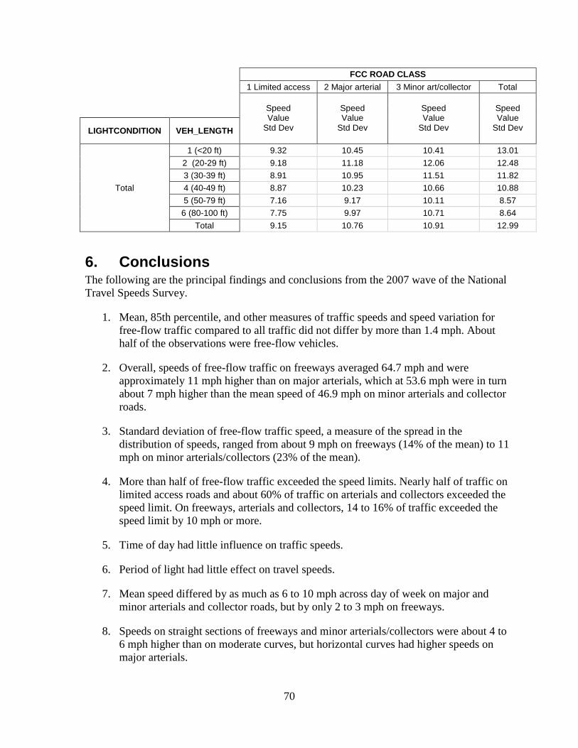
70
FCC ROAD CLASS 1 Limited access 2 Major arterial 3 Minor art/collector Total
Speed Value
Std Dev
Speed Value
Std Dev
Speed Value
Std Dev
Speed Value
Std Dev
LIGHTCONDITION VEH_LENGTH
Total
1 (<20 ft) 9.32 10.45 10.41 13.01 2 (20-29 ft) 9.18 11.18 12.06 12.48 3 (30-39 ft) 8.91 10.95 11.51 11.82 4 (40-49 ft) 8.87 10.23 10.66 10.88 5 (50-79 ft) 7.16 9.17 10.11 8.57
6 (80-100 ft) 7.75 9.97 10.71 8.64 Total 9.15 10.76 10.91 12.99
6. Conclusions The following are the principal findings and conclusions from the 2007 wave of the National Travel Speeds Survey.
1. Mean, 85th percentile, and other measures of traffic speeds and speed variation for free-flow traffic compared to all traffic did not differ by more than 1.4 mph. About half of the observations were free-flow vehicles.
2. Overall, speeds of free-flow traffic on freeways averaged 64.7 mph and were approximately 11 mph higher than on major arterials, which at 53.6 mph were in turn about 7 mph higher than the mean speed of 46.9 mph on minor arterials and collector roads.
3. Standard deviation of free-flow traffic speed, a measure of the spread in the distribution of speeds, ranged from about 9 mph on freeways (14% of the mean) to 11 mph on minor arterials/collectors (23% of the mean).
4. More than half of free-flow traffic exceeded the speed limits. Nearly half of traffic on limited access roads and about 60% of traffic on arterials and collectors exceeded the speed limit. On freeways, arterials and collectors, 14 to 16% of traffic exceeded the speed limit by 10 mph or more.
5. Time of day had little influence on traffic speeds.
6. Period of light had little effect on travel speeds.
7. Mean speed differed by as much as 6 to 10 mph across day of week on major and minor arterials and collector roads, but by only 2 to 3 mph on freeways.
8. Speeds on straight sections of freeways and minor arterials/collectors were about 4 to 6 mph higher than on moderate curves, but horizontal curves had higher speeds on major arterials.

9. Speeds on flat sections of freeways were about 2 to 4 mph higher than on moderate or steep hills. Speeds on steep hills on minor arterials/collectors were about 5 to 6 mph lower than on flat or moderately hilly sections, while speeds on vertical curves on major arterials were 2 to 3 mph higher than on flat sections.
10. Speeds were lowest on urban roads and highest on rural roads of all types. Rural traffic was about 12 to 14 mph faster than urban traffic.
11. Speeds of passenger vehicle and light truck size classes (up to 29 ft.) were generally higher than for medium trucks (30 to 49 ft.). On all road types, speeds of large trucks (50 ft. or more) were higher than medium trucks, and in some circumstances, large truck speeds were higher than passenger vehicles.
12. There is an interaction among curvature (both horizontal and vertical), road class, and vehicle size. In general, speeds decrease as curvature and gradient increase, especially for the largest trucks on minor arterials/collectors.
13. There was little influence of light condition on speed across combinations of passenger vehicle size and road type. Nighttime speeds of the largest trucks were about 1 to 2 mph higher than during daytime on major and minor arterials, but were about the same day and night on freeways.
14. The sample design was less than optimal for estimating speeds. Because the design was a compromise to support both speed estimation and crash risk analysis, PSUs or sites within PSUs were not selected in a way that minimized error variance. A sample redesign should be considered for future waves to improve the speed estimates. The optimal design for general speed analysis is to have equal sampling rates and equal weights for every site. The over-sampling of crash sites resulted in a smaller sample of non-crash sites (assuming a fixed overall sample size) and differential weights between crash and non-crash sites, thereby increasing the variance for estimates that are not specific to crash sites.
15. The survey confirmed the feasibility of estimating travel speeds using a probability sample of measurement sites and uniform procedures for measuring speeds. More than 10 million observations of speeds were recorded of all vehicle types on freeways, major arterials and minor arterials and collector roads with various combinations of horizontal and vertical curvature.
16. The sub-study of the feasibility of measuring speeds at intersections where crashes occurred indicated that although speeds could be measured in each lane, damage and loss of measurement devices was substantially higher and risk of injury to field personnel was elevated at intersections, thus continuation of intersection measurements is not recommended.
71
72
References Shelton, T. S. T. (1991, December). National Accident Sampling System General Estimates
System Technical Note, 1988 to 1990. (Report No. DOT HS 807 796). Washington, DC: National Highway Traffic Safety Administration. Available at www-nrd.nhtsa.dot.gov/Pubs/807796.pdf

73
Appendices

74
Appendix A. Details of Sample Design Logic
The sample design needed to accommodate and support a dual analytical requirement – to provide reliable national estimates of speeds and to determine the relationship between speeds and crashes. Considerable work was required to determine the analytical methodology. Basically, it involved a regression analysis to generate speed distributions for a set of roadway sites. The intent was to match crashes that were associated with a combination of variables with estimated speed distributions for roads having a similar combination of variables. If speed causes crashes, then the speed when crashes occur should be greater than the normal speed for matched roads. The logic behind the analytical approach is:
Let Fr and Fc represent the estimated speed distributions for the matched set of road segments from the regression model and from crashes, respectively. We wish to calculate the excess (or reduced) risk of driving above some speed value, V, by comparing the odds of a crash being above V to the odds of traffic being above V:
OR(V) = [1 – Fc(V)/Fc(V)]/[1 – Fr(V)/Fr(V)] OR(V) will be greater than 1.0 or lower than 1.0 according to whether speeds above V increase or reduce the risk of crashes relative to speeds below V.
One major problem with this approach is that crash and roadway data may not include all of the most important characteristics that affect speed and crashes. This analytical approach requires that “rare” road situations, such as roads with high horizontal and vertical curvature, have adequate representation in the sample.
At the most basic level, the national survey of speeds needs to support estimates of speeds for all characteristics of roads, road users, and geographic locations where speed differences would be of interest. The following characteristics are therefore of interest:
· Region of the country: The United States may be divided into geographic regions where geography, weather, and terrain may have a role in road speeds. Four regional classifications come to mind quickly.
1. There are 10 NHTSA regions, which administer NHTSA programs and also represent some differences in geography and weather. The NOPUS provides estimates of occupant restraint use for each of these regions.
2. The United States could be divided into six regions that represent a combination of geography, terrain and weather patterns. They are: North East, South East, North Central, South Central, North West, and South West.
3. A more compact but somewhat less meaningful four-way regional division of the United States by geography would be North East, South East, North West and Middle/Central.
4. A simple three-way geographic division could be East, Central, and West. The four-way regional classification was selected for sample design.

75
· Roadway type: Several road taxonomies use engineering design features and the character of service they provide to classify roads. The two most applicable are:
1. FHWA Functional Classification System: Roads are divided into urban, small urban, and rural areas and Arterial, Collector and Local road types. The classifications are:
·
·
Rural o Principal Arterial
§ Interstate
§ Other Principal Arterials
o Collectors
§ Major Collector Roads
§ Minor Collector Roads
o Local Roads
Urban and Small Urban o Principal Arterials
§ Interstate
§ Other Freeways and Expressways
§ Other Principal Arterials (no access control)
o Minor Arterials
o Collectors
o Local streets
2. GIS Feature Class Code system: Various geographic information system (GIS) databases (e.g., TANA/GDT4) provide detailed roadway network data organized by feature class codes (FCC). The FCCs of interest for a national speed study include:
·
·
·
·
A10-Primary interstate highway, major category
A20-Primary U.S. and State highways, major category
A30-Secondary State and County highways, major category
A40-Local, neighborhood, rural road, city street, major category The GIS Feature Class Code classification was chosen for the sample design.
Crash characteristics were also a necessary component of the sample design to support association between speeds and crashes. Crash characteristics were to be obtained from
4 2005 Tele Atlas North America, Inc. /Geographic Data Technology Inc.

76
NMVCCS cases that had occurred in each PSU because that crash sample included estimates of pre-crash speeds as part of its data collection procedures. The annual documentation of crashes NASS teams conduct in each PSU was to have been obtained from participating jurisdictions, as well. Sample selection would therefore have needed to account for the following crash characteristics:
·
·
·
·
·
·
Speed related or not speed related;
Horizontal and vertical curvature;
Intersection or non-intersection;
Road design features (presence of shoulders, clear roadside area, ditches, and obstacles, such as poles, trees, culvert, etc.);
Lighted or unlighted; and
Others. Ultimately, this effort featured a three-stage sample design. In the first stage of sampling, primary sampling units were selected. Next, sites for documentation in Phase I of the field work were sampled. Finally, a subsample of eligible sites was selected for speed data collection in Phase II of the field work.
Population: The population consisted of all motor vehicles on all minor and major arterial road segments and collectors, including limited access roads, but excluding local residential streets. Sample PSUs: The set of sample PSUs for this survey were nearly all of those selected for the NMVCCS by NHTSA. A PSU is defined as a central city, the part of a county surrounding a central city, an entire county, or a group of contiguous counties. The NMVCCS sample was selected as a subsample of the NASS GES. The GES sample selection is documented in Shelton (1991). There are 60 sample PSUs in GES and 24 sample PSUs in NMVCCS. These PSUs were used because there is detailed information on crash cause in NMVCCS sample PSUs. A second advantage in using NMVCCS PSUs was a substantial savings in time and cost over a completely independent sample of PSUs, for which analyzing road segment characteristics and obtaining data on crashes would be extremely difficult.
Unfortunately, the NMVCCS data set was not finalized and available before this project concluded. Thus, analysis relating speed to crash incidence was impossible.
The probability of selection for a NMVCCS PSU is roughly proportional to the estimated number of highway crashes with injuries as reported to police in 1983. We concluded that an ideal measure of size for a PSU for this effort was a function of several variables: number of crashes, population of the PSU, and most importantly the number of arterial and limited access highway miles. Miles were most important because the second stage of sampling involved selection of sites along the PSU roads (excluding local roads). Crashes were also important because the survey was particularly interested in the relationship between crashes and speed. A PSU with a relatively high ratio of population to road miles would be likely to

77
have a higher rate of crashes because of more congested roads, which would make population/miles another indicator of crashes.
The correlation between the NMVCCS PSU probabilities of selection, based on a measure of size of 1983 crashes, and the ideal probability of selection, based on a measure of size using miles, population, and current crashes, is only moderate. A PSU with a relatively high number of miles of non-local roads but relatively low 1983 fatal and injury crashes would have large weights for collected data as long as the number of sample sites was the same in each sample PSU, causing some extreme variations in weights across PSUs. Westat alleviated this problem in two ways: sub-sampling of a few PSUs and varying the number of sites per PSU. We determined the ideal number of sample sites per PSU such that this number would be proportional to the ratio of a measure of size using miles, population, and crashes to the NMVCCS PSU measure of size. In doing this, we obtained a highly variable number of desired sites for different PSUs (in terms of the target sample size for Phase I). The PSU with the smallest number of desired sample sites was not included in TSS, resulting in a negligible amount of undercoverage. We selected two of the five PSUs with the next smallest desired number of sample sites with probability proportional to the desired sample size. The three non-selected PSUs were excluded from the sample, with the sample size in the two selected PSUs increased to account for the full set of five PSUs. Thus, this effort was conducted in 20 of the 24 NMVCCS sample PSUs.
Selection of sites for Phase I: Variables related to crashes include road curvature, gradient, super elevation, traffic volume, at or not at intersection, type of road, and weather conditions. The analytical procedure used for this effort required oversampling to ensure that an adequate number of “rare” situations, e.g., highly curved roads, would be represented in the final dataset.
The sample design was conducted in two stages. In this inaugural wave of the survey, it was unknown which segments were gradient/curves in each PSU, consequently more segments than needed were sampled during the Phase I site documentation. In that phase, senior field staff visited each sampled segment, determined whether a Hi-Star could be placed at a site, classified it in terms of gradient and horizontal curvature, and marked the beginning of the segment so that it could be easily located in Phase II data collection if the site was drawn for speed data collection. At the same time, the staff member’s GPS-equipped computer precisely tracked and recorded the person’s geographic position and elevation as he/she drove through each segment.
Roadways were put into one of three classifications. An “intersection site” consisted of the part of each road that was within 150 feet of an intersection. If there were two or more intersections that were within 150 feet of each other, they constituted a single intersection site. Each “mid-block” length of road outside of intersections was divided into one or more segments such that no segment was more than 500 feet long. A “crash site” consisted of a portion of a road or roads where there was a NMVCCS-reported crash that did not occur within an intersection site. All other “mid-block” sites were classified as “non-crash site.”
Intersection speeds and crashes are problematic, in that speed is likely to be buried among many other causal factors in intersection crashes, and the problem of where to measure speed

78
is greater than for non-intersections. Thus, only a small pilot study of intersections was conducted for the present survey. Two intersection sites were selected in each sample PSU for experimental purposes. The plan was to have approximately one-third of the remaining sample sites in a PSU be crash sites and two-thirds non-crash sites. The sample size for non-intersections was set according to what would yield approximately equal weights across PSUs. However, a somewhat smaller target sample size was used for PSUs with very large desired sample sizes, and somewhat larger target sample sizes were used for PSUs with very small desired sample sizes. This was done to avoid field staff being in a sample PSU for an inordinately long period of time or an extremely short period of time. In general, all crash sites where there was information from the police report that speed or aggressive driving was a factor in the reported crash(es) were included in the sample. A sample of other crash sites was selected to obtain the pre-determined number of sample crash sites in each PSU. For every PSU, at least one crash site that was not related to speed/aggressive driver crashes was selected. Crash sites within a PSU were each selected with equal probability, while non-crash sites were selected with probability proportional to length.
Selection of sites for Phase II: The curvature/gradient data collected in Phase I were used to classify a non-crash site as curvy/high gradient (CG) site, or non-curvy/low gradient (non-CG) site. CG sites were those that were at or above a certain threshold for curvature or/and were at or above a certain threshold for gradient. Non-CG sites were those that did not meet the threshold level for curvature or gradient. Sites for which field staff concluded a Hi-Star could not be placed were considered non-responding sites. All other crash sites and CG sites were included in the Phase II sample. Non-CG sites were subsampled to obtain the pre-determined total sample size for a given PSU.

79
Appendix B. Hi-Star Specifications & Manufacturer Validation
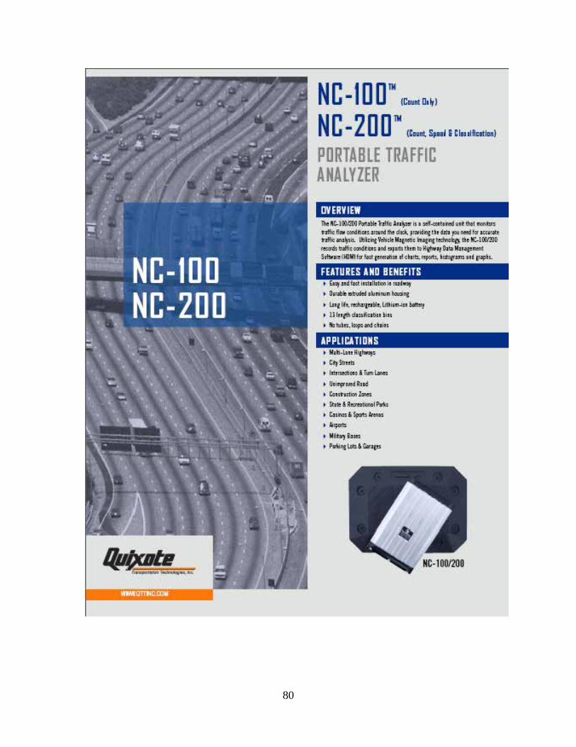
80

81
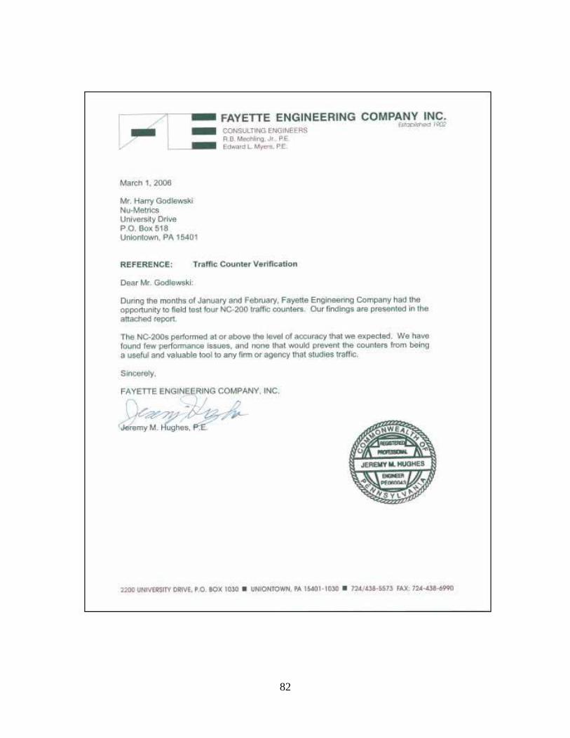
FAYETTE ENGINEERING COMPANY INC.
-
f.-;~1@ CONSULTING ENGINEERS R.O Mect<ling, Jr f)£ £ctw~mJ L Myers. PE
82
March 1, 2006
Mr. Hany Godlewst<i Nu·l'.Wtrlcs Unlvers!ty Orlve P 0 . &ox 518 UniOntown, PA 15401
REFERENCE: TraMe Counter Verification
Dear Mr.. Godlewski:
Dunng the months o1 January ancJ February, Fayette Engineering Company had the opportunity to field test fou,. NC-200 traffte counters.. Our findings ace prosant<td In lhe attached repon.
The NC..200s performed at or above the !(Wt)l of ;.\OCuracy That we expected. We have found few perfonnance i&sues. and none that wt>uld prevent l:he counters from being a useful and va!~bte tool to any firm or agency that studies traffic.
S.in~rcty,
FAYETTE ENG!Nel'RING COMPANY. INC.
~-?Jf·)L_, 2 <JeiemyM. Hughe~7/,_
l200utavtRSITYDRIVt. PO. !QX 1030 • UNIOOTOWN. PA 1MOH 03G • 124/4.36·S51S FAX: 72A·436-4990

83
Introduction
Curing the month$ of January and February. 2006, hyene Engineering Company had the opportunitY to fletd te,. four NC-200 trarr.c counters. The following is a description of our findl"'gs.
Free Flow Test
On January HI, :lOUIS, trom l l ::JU tO 1:30 pm. we conaucted a ttatftc cwnt wilh lh'=' fOur NC200s on SR 119 Noc1hbound. nght tane. approximately 150 yards south of tho intersection of SR 119 and Ml Braddock Road. We simultaneously ooOOuct&d a count with n pennanent loop style counter in the same location. and made a video of tho study. The counters were placed in the center of the lane, and tMthin the loop. After oorr&etlng the clocks on the NC200S and the loop to the time on the cameta. and truncating the count to onty the .-na when all stx de\lices were running, the extent of the stvdy was from 12:29:43 to 1:29:22. Oul1ng this time. 486 vohidOS were observed by the camera to have passed over the counters and loop. The loop reported 487 V(lhlcles (plus 2 ~errors" corresponding to truc::ts passing by in the adjacent lane). The one vehicle discrepancy wQS dve to two vehicles in the adjacent lane being counted and one vehicle ., the s.tvdy lane being missed. The fll'$1 through fourth counters reported 488, 489. 489. and 490 vehk::IC$ .. respectivety. ThO error of the fnt covnter was due to 4 tractor-trailers and 1 llghllruck 1 boat having the tractor and the trailet counted as separate vehicles., and 3 empcy flatbed truck& being missed ontirely. The errors on the second and third counters were due to 5 tractor trailers and 1 light truck 1 boat being counted as separate vehides. and the same 3 flatbeds being m issed. The error on the forth oovnter was due to the same 6 vehicies being cou.V.ed sep,al'l!ltely, and 2 of the previOusly mentioned flatbeds being missed. All three of the mb:sed flatbed trucks had timber beds. In this study. the NC.o-200 countcr.s h<Jd ~;:~n i;:IVI:'I ti'Jt:: vt::hi...., vuvuti•'IW CI«N•·ac.y of 99.4%. The nature of Ofl'O($ for ttle loop and NC200s drffered. Fal.se positives for the loop were due to vehicles in adjacent lanes being counted. whereas false pos&tives for the NC200s were all due to double coundng of long vehicles. The reason for the missed vehide on the loop is not known, although it can be noted that a vehicle 4 seconds behind an ·error" reading was the one that was missed. The three mls.~s for the NC200s were ell tractor traitors with empty timber trailel'$.
Other Field Testing
The fout counters were used to conduce a one day test on a rural road in Gorman Township, Fayette County. Three counters wore placed In one direction and one was placed in the other direction. The paved width of the road is about 14' to 18' and cal'$ tend to dti ... e in the oenter of the road unless another vehlde ts com.,g the other way. The weather was dear. and the tempe..ature was below freezing for the
1
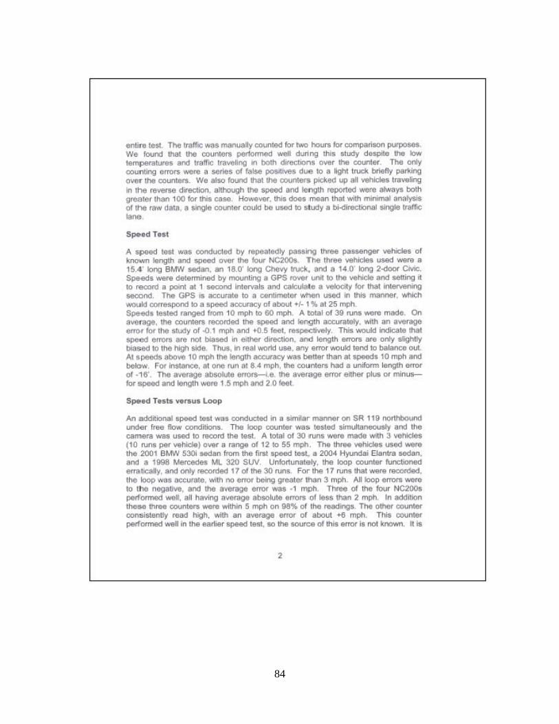
84
entiro IG$t. The troffJC was manually oounted for two hours for comparison purposes. We found that the Cl>unters perfonned well during this study despite the lOw temperatures and traffic troveUng In both directions over the counter. The 1>nly counting errors were o series o.f false posllrves due to a li"'t truck briefly parking over the coooters. We also found that the counters picked up all vehicles traveling In the reverse direction, although the speed and klngth tcported wete atways both gteater than 100 for this ca-se. However, this does mean that with minimal ;:m~tysls ot the raw data, a single counter ooold be used to study a bi -directional Single ttaffJC tano.
Speoed Te.st
A speed test was concluctod by repe.atedly !XISSing three pas~nger vehicles of known 5ength and speed over the tour NC200S. The three vehicles used were a 15.4' iong BMW sedan. an 18.0' k>ng Chevy truck. af"'d a 14 0' long 2-door Civic. Spe-eds were de1ermined by mounting a GPS ro"'Ot vnit 10 the vehicle and setting it to reoord a point at 1 seoond intervals and calcui.2Jl e a velocity for that lntervenWlg second. The GPS is accurate to a centimeter when used in thiS manner, v.tllch would correspond to a speed accuracy of about +/- 1 % at 25 mph. Spe-eds tested ranged from 10 mph to GO mph. A t otal of 39 runs were mode. On average, the counlers recorded the speed and ~ngth aocurately, with an average CttOt for the study of .().1 mph and +0.5 feet, respedively. This would indicate that speed errors are not biased In either d1recllon, and length errors are only slightty biased to the hlgt'l side. Thus, in real world use, any error would tend to balance out. At speeds abc>ve 10 mph the ~ngth l;lOOUracy was better than at speeds 10 mph and belcw. For in.,.ance, at ooe run a1 8.4 mph, the cou nters had a uniform length error ol · 16'. The average absOlute eaors-t.e . the aver~ge error either plus or minusfor speed and length were 1.5 mph and 2.0 feet
Speed T&sts versus loop
An a dditional speed test was conducted in a similar manner on SR 119 northbOund under free flow conditions. The loop oountec was l&$lod simultaneously and tile camera was used to record the test. A total of 30 l"uns were made with 3 vehicles (10 runs per vehicle) over a range of 12 to 55 mph . The three vehicles used .... -are the 2001 BMW 5301 sedan from the first speed test~ a 2004 Hyundai Elantra sedan, and a 1998 Mercedes Ml 320 SUV. Unfortunately, the loop counter functioned erratJcally, and onty recorded 17 of the 30 runs. For the 17 runs that were recorded, the loop was accurate, Wtth no error being greater ltlan 3 mph. All k>op errors Y~'ere to the negatiVe. and the avetage error was ·1 mph. Ttvee of the fovr NC200s performed wei . all having average absolute errors of tess than 2 mph, In addition these three oounters were within 5 mph on 98% of the readings.. The other counter oonsistentty read high, with an average error of abOut +6 mph. This countet performed wei in the earl ier speed test, so the source ol this error is not knoYm. It iS
2

85
JXISSible thai l.he counter was not oriented el(aetly v.i1h the flow of traffic. but this possibility can not be verifted.
Conclusion The NC20()s performed al or above the level of accuracy that we expected. We have found few performanoo iUves, and none that would prevent the counteffl from beJng a useful and valuable toot to any tlrm oc agency thai studies traffiC.
3

DOT HS 811 663August 2012
8633-082312-v3a