I N S T I T U T E F O R D E F E N S E A N A L Y S E S

December 2015

Approved for public release; distribution is unlimited.

IDA Paper NS P-5308Log: H 15-001016

NATO Allied Medical Publication 7.5 Study Draft 3 (AMedP-7.5 SD.3),

“NATO Planning Guide for the Estimation of CBRN Casualties”

Carl A. Curling, Project LeaderSean M. Oxford

The information contained in this document shall not be released to a nation outside of NATO without following procedures contained in C-M(2002)60.

INSTITUTE FOR DEFENSE ANALYSES4850 Mark Center Drive

Alexandria, Virginia 22311-1882

About This PublicationThis work was conducted by the Institute for Defense Analyses under contract HQ0034-14-D-0001, Project CA-6-3079, “CBRN Casualty Estimation Update of the Medical CBRN Defense Planning & Response Project,” for the Office of the Surgeon General of the Army and the Joint Staff, Joint Requirements Office for CBRN Defense (J-8, JRO). The publication of this IDA document does not indicate endorsement by the Department of Defense, nor should the contents be construed as reflecting the official position of that Agency.

AcknowledgementsThe author thanks Mr. Doug Schultz, Mr. Mark Tillman, and Ms. Julia Burr for their guidance and helpful comments.

Copyright© 2015 Institute for Defense Analyses, 4850 Mark Center Drive, Alexandria, Virginia 22311-1882 • (703) 845-2000.

This material may be reproduced by or for the U.S. Government pursuant to the copyright license under the clause at DFARS 252.227-7013 (a)(16) [Jun 2013].

The Institute for Defense Analyses is a non-profit corporation that operates three federally funded research and development centers to provide objective analyses of national security issues, particularly those requiring scientific and technical expertise, and conduct related research on other national challenges.

I N S T I T U T E F O R D E F E N S E A N A L Y S E S

IDA Paper NS P-5308

NATO Allied Medical Publication 7.5 Study Draft 3 (AMedP-7.5 SD.3),

“NATO Planning Guide for the Estimation of CBRN Casualties”

Carl A. Curling, Project LeaderSean M. Oxford

The information contained in this document shall not be released to a nation outside of NATO without following procedures contained in C-M(2002)60.

The information contained in this document shall not be released to a nation outside of NATO without following procedures contained in C-M(2002)60.

NATO STANDARD

AMedP-7.5

NATO PLANNING GUIDE FOR THE ESTIMATION OF CBRN CASUALTIES

EDITION A VERSION 1 STUDY DRAFT 3

MARCH 2016

NORTH ATLANTIC TREATY ORGANIZATION

ALLIED MEDICAL PUBLICATION

Published by the NATO STANDARDIZATION OFFICE (NSO)

© NATO/OTAN

INTENTIONALLY BLANK

NORTH ATLANTIC TREATY ORGANIZATION (NATO)

NATO STANDARDIZATION OFFICE (NSO)

NATO LETTER OF PROMULGATION

[Date]

1. The enclosed Allied Medical Publication AMedP-7.5, NATO Planning Guide forthe Estimation of CBRN Casualties, which has been approved by the nations in the [TA], is promulgated herewith. The agreement of nations to use this publication is recorded in STANAG 2553.

2. AMedP-7.5(A) is effective upon receipt and supersedes AMedP-8(C), whichshall be destroyed in accordance with the local procedure for the destruction of documents.

3. No part of this publication may be reproduced, stored in a retrieval system, usedcommercially, adapted, or transmitted in any form or by any means, electronic, mechanical, photo-copying, recording or otherwise, without the prior permission of the publisher. With the exception of commercial sales, this does not apply to member nations and Partnership for Peace countries, or NATO commands and bodies.

4. This publication shall be handled in accordance with C-M(2002)60.

Edvardas MAŽEIKISMajor General, LTUAF Director, NATO Standardization Office

INTENTIONALLY BLANK

AMedP-7.5

I SD.3

RESERVED FOR NATIONAL LETTER OF PROMULGATION

AMedP-7.5

II SD.3

INTENTIONALLY BLANK

AMedP-7.5

III SD.3

RECORD OF RESERVATIONS

CHAPTER RECORD OF RESERVATION BY NATIONS

Note: The reservations listed on this page include only those that were recorded at time of promulgation and may not be complete. Refer to the NATO Standardization Document Database for the complete list of existing reservations.

AMedP-7.5

IV SD.3

INTENTIONALLY BLANK

AMedP-7.5

V SD.3

RECORD OF SPECIFIC RESERVATIONS

[nation] [detail of reservation]

Note: The reservations listed on this page include only those that were recorded at time ofpromulgation and may not be complete. Refer to the NATO Standardization Document Databasefor the complete list of existing reservations.

AMedP-7.5

VI SD.3

INTENTIONALLY BLANK

AMedP-7.5

VII SD.3

TABLE OF CONTENTS

CHAPTER 1  DESCRIPTION OF THE METHODOLOGY ..................................... 1-1 1.1.  INTRODUCTION AND DOCUMENT ORGANIZATION ............................. 1-1 1.2.  PURPOSE AND INTENDED USE .............................................................. 1-2 1.3.  SCOPE ........................................................................................................ 1-3 1.3.1.  Challenge Types .................................................................................. 1-4 1.3.2.  Types of Casualty ................................................................................ 1-6 1.3.3.  Countermeasures ................................................................................ 1-6 1.4.  DEFINITIONS ............................................................................................. 1-7 1.4.1.  Types of Casualty .............................................................................. 1-10 1.5.  GENERAL ASSUMPTIONS, LIMITATIONS, AND CONSTRAINTS ........ 1-12 1.6.  SUMMARY OF THE METHODOLOGY .................................................... 1-12 1.6.1.  INPUT ................................................................................................ 1-13 1.6.2.  CHALLENGE ..................................................................................... 1-14 1.6.3.  RESPONSE and STATUS ................................................................. 1-15 1.6.4.  REPORT ............................................................................................ 1-17 1.6.5.  User Aids ............................................................................................ 1-18 CHAPTER 2  USER INPUT .................................................................................... 2-1 2.1.  ICONS AND ICON ATTRIBUTES ............................................................... 2-1 2.1.1.  Overview of Icon Attributes .................................................................. 2-1 2.1.2.  CBRN Challenge or Effective CBRN Challenge .................................. 2-3 2.1.3.  Breathing Rate ..................................................................................... 2-6 2.1.4.  Body Surface Area ............................................................................... 2-6 2.1.5.  Individual Protective Equipment (IPE) ................................................. 2-7 2.1.6.  Vehicles and Shelters (Physical Protection and ColPro) ..................... 2-7 2.1.7.  Pre-Exposure Prophylaxis ................................................................. 2-10 2.1.8.  Uniform ............................................................................................... 2-11 2.1.9.  Aggregate Protection Factor .............................................................. 2-11 2.1.10.  Example Input and Comparison of Input Schemes ........................... 2-11 2.2  METHODOLOGY PARAMETERS ............................................................ 2-14 CHAPTER 3  EFFECTIVE CBRN CHALLENGE ESTIMATION ............................ 3-1 3.1.  INPUT SCHEME 1 ...................................................................................... 3-1 3.2.  INPUT SCHEME 1 WITH TOXIC LOAD FOR CHEMICAL AGENTS ........ 3-4 3.3.  INPUT SCHEME 2 ...................................................................................... 3-5 CHAPTER 4  CHEMICAL, RADIOLOGICAL, AND NUCLEAR HUMAN RESPONSE

AND CASUALTY ESTIMATION ...................................................... 4-1 4.1.  CRN MODEL FRAMEWORK ...................................................................... 4-1 4.1.1.  Human Response—Injury Profiles (CRN) ........................................... 4-1 4.1.2.  Assignment of Personnel to Injury Profiles .......................................... 4-4 4.1.3.  Casualty Estimation ............................................................................. 4-8 4.2.  CHEMICAL AGENT MODELS .................................................................. 4-11 4.2.1.  Assumption and Constraint ................................................................ 4-11 4.2.2.  GA ...................................................................................................... 4-11 4.2.3.  GB ...................................................................................................... 4-13 4.2.4.  GD ...................................................................................................... 4-16 

AMedP-7.5

VIII SD.3

4.2.5.  GF ...................................................................................................... 4-18 4.2.6.  VX ...................................................................................................... 4-21 4.2.7.  HD ...................................................................................................... 4-25 4.2.8.  CG ...................................................................................................... 4-31 4.2.9.  Cl2 ....................................................................................................... 4-34 4.2.10.  NH3 ..................................................................................................... 4-36 4.2.11.  AC ...................................................................................................... 4-38 4.2.12.  CK ...................................................................................................... 4-41 4.2.13.  H2S ..................................................................................................... 4-43 4.3.  RADIOLOGICAL AGENT MODELS ......................................................... 4-46 4.3.1.  Assumptions and Limitation ............................................................... 4-46 4.3.2.  RDDs .................................................................................................. 4-46 4.3.3.  Fallout ................................................................................................ 4-52 4.3.4.  Threshold Lethal Dose and Time to Death ........................................ 4-55 4.3.5.  Dose Ranges, Injury Profiles, and Medical Treatment Outcomes .... 4-56 4.4.  NUCLEAR EFFECTS MODELS ............................................................... 4-58 4.4.1.  Assumptions and Limitations ............................................................. 4-58 4.4.2.  Initial Whole-body Radiation .............................................................. 4-58 4.4.3.  Blast ................................................................................................... 4-61 4.4.4.  Thermal Fluence ................................................................................ 4-64 CHAPTER 5  BIOLOGICAL HUMAN RESPONSE AND CASUALTY ESTIMATION

.......................................................................................................... 5-1 5.1.  BIOLOGICAL AGENT MODEL FRAMEWORK .......................................... 5-1 5.1.1.  Human Response Submodels ............................................................. 5-1 5.1.2.  Casualty Estimation ............................................................................. 5-3 5.1.3.  Assumptions and Limitations ............................................................... 5-3 5.1.4.  Non-Contagious Casualty Estimation .................................................. 5-3 5.1.5.  Contagious Casualty Estimation .......................................................... 5-9 5.1.6.  Equations Needed to Execute Casualty Estimates ........................... 5-17 5.2.  BIOLOGICAL AGENT MODELS ............................................................... 5-18 5.2.1.  Anthrax ............................................................................................... 5-18 5.2.2.  Brucellosis .......................................................................................... 5-33 5.2.3.  Glanders ............................................................................................. 5-43 5.2.4.  Melioidosis ......................................................................................... 5-50 5.2.5.  Plague (non-contagious model) ......................................................... 5-55 5.2.6.  Plague (contagious model) ................................................................ 5-59 5.2.7.  Q Fever .............................................................................................. 5-60 5.2.8.  Tularemia ........................................................................................... 5-64 5.2.9.  Smallpox (non-contagious model) ..................................................... 5-69 5.2.10.  Smallpox (contagious model) ............................................................ 5-73 5.2.11.  Eastern Equine Encephalitis Virus (EEEV) Disease ......................... 5-74 5.2.12.  Venezuelan Equine Encephalitis Virus (VEEV) Disease ................... 5-76 5.2.13.  Western Equine Encephalitis Virus (WEEV) Disease ....................... 5-78 5.2.14.  Botulism ............................................................................................. 5-80 5.2.15.  Ricin Intoxication ................................................................................ 5-89 5.2.16.  Staphylococcal Enterotoxin B (SEB) Intoxication .............................. 5-92 

AMedP-7.5

IX SD.3

5.2.17.  T-2 Mycotoxicosis .............................................................................. 5-95 5.2.18.  Ebola Virus Disease ........................................................................... 5-97 CHAPTER 6  CASUALTY SUMMATION AND REPORTING ................................ 6-1 6.1.  APPLICATION OF AJP-4.10 REQUIREMENTS ........................................ 6-1 6.2.  DESCRIPTION OF OUTPUT REPORTING ............................................... 6-2 6.3.  PERSONNEL STATUS TABLE FOR NUCLEAR CASUALTIES ............... 6-5 ANNEX A  ILLUSTRATIVE EXAMPLES ........................................................... A-1 A.1.  OVERVIEW ................................................................................................ A-1 A.2.  INPUT (ALL ILLUSTRATIVE EXAMPLES) ................................................ A-1 A.2.1.  Icons and Icon Attributes .................................................................... A-2 A.2.2.  Methodology Parameters .................................................................. A-14 A.3.  CHEMICAL AGENT: GB .......................................................................... A-14 A.3.1.  INPUT ............................................................................................... A-15 A.3.2.  CHALLENGE .................................................................................... A-17 A.3.3.  RESPONSE/STATUS ....................................................................... A-19 A.3.4.  REPORT ........................................................................................... A-22 A.4.  CHEMICAL AGENT: CK .......................................................................... A-24 A.4.1.  INPUT ............................................................................................... A-26 A.4.2.  CHALLENGE .................................................................................... A-27 A.4.3.  RESPONSE/STATUS ....................................................................... A-28 A.4.4.  REPORT ........................................................................................... A-32 A.5.  RDD: 137CS ............................................................................................... A-34 A.5.1.  INPUT ............................................................................................... A-36 A.5.2.  CHALLENGE .................................................................................... A-37 A.5.3.  RESPONSE/STATUS ....................................................................... A-39 A.5.4.  REPORT ........................................................................................... A-40 A.6.  NUCLEAR DETONATION: 10 KT GROUND BURST ............................. A-42 A.6.1.  INPUT ............................................................................................... A-45 A.6.2.  CHALLENGE .................................................................................... A-46 A.6.3.  RESPONSE/STATUS ....................................................................... A-51 A.6.4.  REPORT ........................................................................................... A-57 A.7.  NON-CONTAGIOUS BIOLOGICAL AGENT: B. ANTHRACIS ................ A-59 A.7.1.  INPUT ............................................................................................... A-59 A.7.2.  CHALLENGE .................................................................................... A-61 A.7.3.  RESPONSE/STATUS ....................................................................... A-62 A.7.4.  REPORT ........................................................................................... A-64 A.8.  CONTAGIOUS BIOLOGICAL AGENT: V. MAJOR ................................. A-67 A.8.1.  INPUT ............................................................................................... A-68 A.8.2.  CHALLENGE .................................................................................... A-69 A.8.3.  RESPONSE/STATUS—Non-Contagious Model .............................. A-69 A.8.4.  REPORT—Non-Contagious Model .................................................. A-71 A.8.5.  RESPONSE/STATUS—Contagious Model ...................................... A-73 A.8.6.  REPORT—Contagious Model .......................................................... A-75 ANNEX B  REFERENCES ................................................................................ B-1 

INTENTIONALLY BLANK

AMedP-7.5

X SD.3

LIST OF FIGURES

Figure 1-1:  Relationship of Casualty Criterion, Injury Severity Level, and WIA ... 1-15 Figure 1-2:  Decision Tree for Assignment of Casualty Category ......................... 1-16 Figure 1-3:  AMedP-7.5(A) Methodology Overview .............................................. 1-19 Figure 4-1:  Flowchart for Generation of Composite Injury Profiles ........................ 4-2 Figure 4-2:  Notional Example of Composite Injury Profile Generation .................. 4-2 Figure 4-3:  Human Response Casualty Estimation Flowchart for GA ................. 4-13 Figure 4-4:  Human Response Casualty Estimation Flowchart for GB ................. 4-15 Figure 4-5:  Human Response Casualty Estimation Flowchart for GD ................. 4-18 Figure 4-6:  Human Response Casualty Estimation Flowchart for GF ................. 4-20 Figure 4-7:  Human Response and Casualty Estimation Flowchart for VX .......... 4-24 Figure 4-8:  Human Response and Casualty Estimation Flowchart for HD .......... 4-30 Figure 4-9:  Human Response and Casualty Estimation Flowchart for CG.......... 4-33 Figure 4-10:  Human Response and Casualty Estimation Flowchart for Cl2 .......... 4-35 Figure 4-11:  Human Response and Casualty Estimation Flowchart for NH3 ........ 4-37 Figure 4-12:  Human Response and Casualty Estimation Flowchart for AC .......... 4-40 Figure 4-13:  Human Response and Casualty Estimation Flowchart for CK .......... 4-43 Figure 4-14:  Human Response and Casualty Estimation Flowchart for H2S ......... 4-45 Figure 4-15:  Human Response and Casualty Estimation Flowchart for RDDs ..... 4-51 Figure 4-16:  Human Response and Casualty Estimation Flowchart for Fallout .... 4-54 Figure 4-17:  Human Response and Casualty Estimation Flowchart for Initial Whole-

Body Radiation From a Nuclear Detonation ...................................... 4-60 Figure 4-18:  Human Response and Casualty Estimation Flowchart for Primary

Nuclear Blast ...................................................................................... 4-63 Figure 4-19:  Human Response and Casualty Estimation Flowchart for Thermal

Fluence From a Nuclear Detonation .................................................. 4-68 Figure 5-1:  Non-Contagious Agent/Disease Casualty Estimation Flowchart ........ 5-4 Figure 5-2:  Interaction of SEIRP Cohorts and Parameters .................................. 5-13 Figure 5-3:  Human Response and Casualty Estimation for Anthrax ................... 5-33 Figure 5-4:  Human Response and Casualty Estimation for Brucellosis .............. 5-43 Figure 5-5:  Human Response and Casualty Estimation for Glanders ................. 5-49 Figure 5-6:  Human Response and Casualty Estimation for Melioidosis .............. 5-55 Figure 5-7:  Human Response and Casualty Estimation for Plague (non-contagious

model) ................................................................................................ 5-59 Figure 5-8:  Human Response and Casualty Estimation for Q Fever ................... 5-64 Figure 5-9:  Human Response and Casualty Estimation for Tularemia ................ 5-69 Figure 5-10:  Human Response and Casualty Estimation Flowchart for Smallpox (non-

contagious model) .............................................................................. 5-73 Figure 5-11:  Human Response and Casualty Estimation Flowchart for EEEV Disease

........................................................................................................... 5-76 Figure 5-12:  Human Response and Casualty Estimation Flowchart for VEEV Disease

........................................................................................................... 5-78 Figure 5-13:  Human Response and Casualty Estimation Flowchart for WEEV Disease

AMedP-7.5

XI SD.3

........................................................................................................... 5-80 Figure 5-14:  Human Response and Casualty Estimation Flowchart for Botulism . 5-88 Figure 5-15:  Human Response and Casualty Estimation Flowchart for Ricin

Intoxication ......................................................................................... 5-92 Figure 5-16:  Human Response and Casualty Estimation Flowchart for SEB

Intoxication ......................................................................................... 5-94 Figure 5-17:  Human Response and Casualty Estimation Flowchart for T-2

Mycotoxicosis ..................................................................................... 5-97 Figure A-1:  Layout of Icons .................................................................................... A-2 Figure A-2:  GB Attack on Task Force .................................................................. A-16 Figure A-3:  CK Attack on Task Force .................................................................. A-27 Figure A-4:  137Cs RDD Attack on Task Force ...................................................... A-37 Figure A-5:  10 kT Ground Nuclear Attack on Task Force ................................... A-46 Figure A-6:  B. anthracis (Anthrax) Attack on Task Force .................................... A-61 Figure A-7:  V. major (Smallpox) Attack on Task Force ....................................... A-69 

AMedP-7.5

XII SD.3

LIST OF TABLES

Table 1-1:  Chemical Agent Challenge Types ....................................................... 1-4 Table 1-2:  Challenge Types and Associated Terminology ................................... 1-8 Table 1-3:  Injury Severity Level Definitions ......................................................... 1-10 Table 1-4:  Casualty Reporting Rules .................................................................. 1-18 Table 1-5:  User’s Roadmap ................................................................................ 1-20 Table 1-6:  Cross-References for AMedP-7.5 and Standards Related Document .. 1-

21 Table 1-7:  Guide to AMedP-7.5 Measurement Units .......................................... 1-22 Table 2-1:  Challenge-Modifying Icon Attributes .................................................... 2-2 Table 2-2:  Challenge Types and Associated Units for CBRN Challenges ........... 2-4 Table 2-3:  Suggested and Default Breathing Rates ............................................. 2-6 Table 2-4:  Suggested IPE Protection Factors ....................................................... 2-7 Table 2-5:  Suggested Air Exchange Rates for Vehicles and Shelters Without ColPro

............................................................................................................. 2-9 Table 2-6:  Suggested Inhalation and Percutaneous Protection Factors for Vehicles

and Shelters ......................................................................................... 2-9 Table 2-7:  Suggested Radiation Shielding Protection Factors for Vehicles and

Shelters .............................................................................................. 2-10 Table 2-8:  Suggested Blast Shielding Protection Factors .................................. 2-10 Table 2-9:  Suggested Protection Factors for CRN Prophylaxis ......................... 2-11 Table 2-10:  Example Definition of Icons ............................................................... 2-12 Table 2-11:  Example Input for Input Scheme 1, for a Notional GB Incident ......... 2-13 Table 2-12:  Example Input for Input Scheme 2, for a Notional GB Incident ......... 2-14 Table 2-13:  Example Differences in Effective CBRN Challenge Resulting from Using

Different Input Schemes for the Same Notional GB Incident ............ 2-14 Table 2-14:  Default Values for User-Specifiable Parameters ............................... 2-15 Table 3-1:  Suggested Dose Conversion Factors for RDDs for Selected Isotopes

(Daughter Products Included)* ............................................................. 3-3 Table 3-2:  Suggested Conversion Factors for Fallout .......................................... 3-4 Table 4-1:  Inhaled GA Toxicity Parameters and Symptoms ............................... 4-12 Table 4-2:  Inhaled GA Injury Profiles .................................................................. 4-12 Table 4-3:  GA Medical Treatment Outcome Reporting ...................................... 4-12 Table 4-4:  Inhaled GB Toxicity Parameters and Symptoms ............................... 4-14 Table 4-5:  Inhaled GB Injury Profiles .................................................................. 4-14 Table 4-6:  GB Medical Treatment Outcome Reporting ...................................... 4-14 Table 4-7:  Inhaled GD Toxicity Parameters and Symptoms............................... 4-16 Table 4-8:  Inhaled GD Injury Profiles .................................................................. 4-17 Table 4-9:  GD Medical Treatment Outcome Reporting ...................................... 4-17 Table 4-10:  Inhaled GF Toxicity Parameters and Symptoms ............................... 4-19 Table 4-11:  Inhaled GF Injury Profiles .................................................................. 4-19 Table 4-12:  GF Medical Treatment Outcome Reporting ....................................... 4-19 Table 4-13:  Inhaled VX Toxicity Parameters and Symptoms ............................... 4-21 Table 4-14:  Inhaled VX Injury Profiles .................................................................. 4-22 Table 4-15:  Percutaneous VX Liquid Toxicity Parameters and Symptoms .......... 4-22 

AMedP-7.5

XIII SD.3

Table 4-16:  Percutaneous VX Liquid Injury Profiles ............................................. 4-22 Table 4-17:  VX Medical Treatment Outcome Reporting ....................................... 4-23 Table 4-18:  Recommended Parameter Values for Equivalent Vapour Conversion

Factors for HD (CFHD,k) ...................................................................... 4-26 Table 4-19:  Inhaled HD Toxicity Parameters and Symptoms ............................... 4-26 Table 4-20:  Inhaled HD Injury Profiles .................................................................. 4-27 Table 4-21:  Ocular HD Vapour Toxicity Parameters and Symptoms ................... 4-27 Table 4-22:  Ocular HD Vapour Injury Profiles ....................................................... 4-27 Table 4-23:  Equivalent Percutaneous HD Vapour Toxicity Parameters and

Symptoms .......................................................................................... 4-28 Table 4-24:  Equivalent Percutaneous HD Vapour Injury Profiles ......................... 4-28 Table 4-25:  HD Medical Treatment Outcome Reporting ...................................... 4-29 Table 4-26:  Inhaled CG Toxicity Parameters and Symptoms............................... 4-31 Table 4-27:  Inhaled CG Injury Profiles .................................................................. 4-31 Table 4-28:  Peak CG Concentration Ranges ....................................................... 4-31 Table 4-29:  Peak CG Concentration Injury Profile ................................................ 4-32 Table 4-30:  CG Medical Treatment Outcome Reporting ...................................... 4-32 Table 4-31:  Inhaled Cl2 Toxicity Parameters and Symptoms ............................... 4-34 Table 4-32:  Inhaled Cl2 Injury Profiles ................................................................... 4-34 Table 4-33:  Cl2 Medical Treatment Outcome Reporting ....................................... 4-35 Table 4-34:  Inhaled NH3 Toxicity Parameters and Symptoms ............................. 4-36 Table 4-35:  Inhaled NH3 Injury Profiles ................................................................. 4-36 Table 4-36:  NH3 Medical Treatment Outcome Reporting ..................................... 4-37 Table 4-37:  Inhaled AC Toxicity Parameters and Symptoms ............................... 4-38 Table 4-38:  Inhaled AC Injury Profiles .................................................................. 4-39 Table 4-39:  AC Medical Treatment Outcome Reporting ....................................... 4-39 Table 4-40:  Inhaled CK Toxicity Parameters and Symptoms ............................... 4-41 Table 4-41:  Inhaled CK Injury Profiles .................................................................. 4-42 Table 4-42:  Peak CK Concentration Ranges ........................................................ 4-42 Table 4-43:  Peak CK Concentration Injury Profiles .............................................. 4-42 Table 4-44:  CK Medical Treatment Outcome Reporting ....................................... 4-42 Table 4-45:  Inhaled H2S Toxicity Parameters and Symptoms .............................. 4-44 Table 4-46:  Inhaled H2S Injury Profiles ................................................................. 4-44 Table 4-47:  H2S Medical Treatment Outcome Reporting ..................................... 4-44 Table 4-48:  Whole-Body Radiation LD50 for Instantaneous Challenges .............. 4-55 Table 4-49:  Cutaneous Radiation Dose Ranges .................................................. 4-56 Table 4-50:  Cutaneous Radiation Injury Profiles .................................................. 4-56 Table 4-51:  Cutaneous Radiation Medical Treatment Outcome Reporting .......... 4-56 Table 4-52:  Whole-Body Radiation Dose Ranges ................................................ 4-57 Table 4-53:  Whole-Body Radiation Injury Profiles ................................................ 4-57 Table 4-54:  Whole-Body Radiation Medical Treatment Outcome Reporting ....... 4-57 Table 4-55:  Primary Nuclear Blast Insult Ranges ................................................. 4-62 Table 4-56:  Primary Nuclear Blast Injury Profiles ................................................. 4-62 Table 4-57:  Primary Nuclear Blast Medical Treatment Outcome Reporting......... 4-62 Table 4-58:  Recommended Thermal Transmission Probabilities for Various Vehicle

and Shelter Types .............................................................................. 4-65 

AMedP-7.5

XIV SD.3

Table 4-59:  Thermal Fluence Threshold Values for Partial-Thickness (Second Degree) Burns for Various Uniform Types ........................................ 4-66 

Table 4-60:  Thermal Fluence Insult Ranges ......................................................... 4-67 Table 4-61:  Thermal Fluence Injury Profiles ......................................................... 4-67 Table 4-62:  Thermal Fluence Medical Treatment Outcome Reporting ................ 4-67 Table 5-1:  Example PDT, “Daily Fraction of Non-Survivors (F) Ill with Example

Disease Who DOW” ............................................................................. 5-7 Table 5-2:  Factors to Consider for User-Specified Parameters .......................... 5-12 Table 5-3:  Guidance on Using SEIRP Equations to Populate Output Tables .... 5-15 Table 5-4:  Anthrax Dose Ranges ........................................................................ 5-19 Table 5-5:  Probability of an Individual Still Being in Stage 1 of Anthrax (Pin-Stg1) After

Specified Durations Spent in Stage 1 ................................................ 5-21 Table 5-6:  Anthrax Injury Profile .......................................................................... 5-21 Table 5-7:  Anthrax Prophylaxis Summary .......................................................... 5-21 Table 5-8:  Anthrax Submodel Summary ............................................................. 5-22 Table 5-9:  Daily Fraction of Individuals Ill with Anthrax (EDR) Who Become WIA, for

Casualty Criterion WIA(1+) or WIA(2+)* .............................................. 5-23 Table 5-10:  Daily Fraction of Individuals Ill with Anthrax (EDR) Who Become WIA, for

Casualty Criterion WIA(3+)* ................................................................ 5-24 Table 5-11:  Daily Fraction of Untreated Anthrax Non-Survivors (FDR,U) Who DOW . 5-

25 Table 5-12:  Daily Fraction of Stage 1 Treated Anthrax Non-Survivors (FDR,T-1) and

Survivors (SDR,T-1) Who Enter Stage 2 ............................................... 5-26 Table 5-13:  Daily Fraction of Stage 1 Treated Anthrax Non-Survivors (FDR,T-1) Who

DOW* ................................................................................................. 5-27 Table 5-14:  Daily Fraction of Stage 1 Treated Anthrax Survivors (SDR,T-1) Who

Become CONV*.................................................................................. 5-28 Table 5-15:  Daily Fraction of Stage 1 Treated Anthrax Survivors (SDR,T-1) Who

Become RTD ..................................................................................... 5-30 Table 5-16:  Daily Fraction of Stage 2 Treated Anthrax Non-Survivors (FDR,T-2) Who

DOW .................................................................................................. 5-31 Table 5-17:  Brucellosis Injury Profile..................................................................... 5-36 Table 5-18:  Brucellosis Submodel Summary ........................................................ 5-36 Table 5-19:  Daily Fraction of Individuals Ill with Insidious Onset Brucellosis (Sins,U,

Sins,T-WIA, Sins,T-1, Sins,T-2) Who Become WIA, for Casualty Criterion WIA(1+); Daily Fraction of Individuals Ill with Abrupt Onset Brucellosis (Sabr,U, Sabr,T-WIA, Sabr,T) Who Become WIA, for any Casualty Criterion* 5-37 

Table 5-20:  Daily Fraction of Individuals Ill with Insidious Onset Brucellosis (Sins,U, Sins,T-2) Who Become WIA, for Casualty Criterion WIA(2+) or WIA(3+)* . 5-37 

Table 5-21:  Daily Fraction of Untreated Insidious Onset Brucellosis Survivors (Sins,U) or Abrupt Onset Brucellosis Survivors (Sabr,U) Who Become RTD* ... 5-38 

Table 5-22:  Daily Fraction of Abrupt Onset Brucellosis Casualties Treated Upon Becoming WIA (Sabr,T-WIA) Who Become CONV*; Daily Fraction of Insidious Onset Brucellosis Casualties Treated Upon Becoming WIA

AMedP-7.5

XV SD.3

(Sins,T-WIA) Who Become CONV, for Casualty Criterion WIA(1+)* ....... 5-39 Table 5-23:  Daily Fraction of Insidious Onset Brucellosis Casualties Treated Upon

Becoming WIA (Sins,T-WIA) Who Become CONV, for Casualty Criterion WIA(2+) or WIA(3+)* ............................................................................ 5-39 

Table 5-24:  Daily Fraction of Abrupt Onset Brucellosis Casualties Treated Upon Becoming WIA (Sabr,T-WIA) Who Become RTD*; Daily Fraction of Insidious Onset Brucellosis Casualties Treated Upon Becoming WIA (Sins,T-WIA) Who Become RTD, for Casualty Criterion WIA(1+)* .......................... 5-40 

Table 5-25:  Daily Fraction of Insidious Onset Brucellosis Casualties Treated Upon Becoming WIA (Sins,T-WIA) Who Become RTD, for Casualty Criterion WIA(2+) or WIA(3+)* ............................................................................ 5-41 

Table 5-26:  Daily Fraction of Stage 1 Treated Brucellosis Survivors (Sabr,T, Sins,T-1) and Stage 2 Treated Brucellosis Survivors (Sins,T-2) Who Become CONV ........................................................................................................... 5-42 

Table 5-27:  Daily Fraction of Stage 1 Treated Brucellosis Survivors (Sabr,T, Sins,T-1) and Stage 2 Treated Brucellosis Survivors (Sins,T-2) Who Become RTD5-42 

Table 5-28:  Glanders Injury Profile ....................................................................... 5-44 Table 5-29:  Glanders Submodel Summary ........................................................... 5-44 Table 5-30:  Daily Fraction of Individuals Ill with Glanders (E) Who Become WIA, for

Casualty Criterion WIA(1+)* ................................................................ 5-45 Table 5-31:  Daily Fraction of Individuals Ill with Glanders (E) Who Become WIA, for

Casualty Criterion WIA(2+)* ................................................................ 5-45 Table 5-32:  Daily Fraction of Individuals Ill with Glanders (E) Who Become WIA, for

Casualty Criterion WIA(3+)* ................................................................ 5-46 Table 5-33:  Daily Fraction of Untreated Glanders Non-Survivors (FU) Who DOW .. 5-

46 Table 5-34:  Daily Fraction of Stage 1 Treated Glanders Survivors (ST-1) Who Enter

Stage 2 ............................................................................................... 5-46 Table 5-35:  Daily Fraction of Stage 1 Treated Glanders Survivors (ST-1) Who Enter

Stage 3 ............................................................................................... 5-47 Table 5-36:  Daily Fraction of Stage 1 Treated Glanders Survivors (ST-1) Who Become

RTD .................................................................................................... 5-47 Table 5-37:  Daily Fraction of Stage 2 Treated Glanders Survivors (ST-2) Who Enter

Stage 3 ............................................................................................... 5-47 Table 5-38:  Daily Fraction of Stage 2 Treated Glanders Survivors (ST-2) Who Become

RTD .................................................................................................... 5-48 Table 5-39:  Daily Fraction of Stage 3 Treated Glanders Survivors (ST-3) Who Become

RTD .................................................................................................... 5-48 Table 5-40:  Melioidosis Injury Profile .................................................................... 5-52 Table 5-41:  Melioidosis Submodel Summary ....................................................... 5-52 Table 5-42:  Daily Fraction of Individuals Ill with Melioidosis (E) Who Become WIA* 5-

53 Table 5-43:  Daily Fraction of Individuals Ill with Melioidosis (E) Who Enter Stage 2 of

Illness* ................................................................................................ 5-53 Table 5-44:  Daily Fraction of Untreated or Treated Melioidosis Non-Survivors (FU, FT-

AMedP-7.5

XVI SD.3

WIA, FT-1, or FT-2) Who DOW ............................................................... 5-53 Table 5-45:  Daily Fraction of Untreated Melioidosis Survivors (SU) Who Become RTD

........................................................................................................... 5-54 Table 5-46:  Daily Fraction of Melioidosis Survivors Treated Upon Becoming WIA (ST-

WIA) Who Become RTD* ..................................................................... 5-54 Table 5-47:  Daily Fraction of Stage 1 Treated Melioidosis Survivors (ST-1) and Stage

2 Treated Melioidosis Survivors (ST-2) Who Become RTD ................ 5-54 Table 5-48:  Plague Injury Profile ........................................................................... 5-57 Table 5-49:  Plague Prophylaxis Summary ............................................................ 5-57 Table 5-50:  Plague Submodel Summary .............................................................. 5-57 Table 5-51:  Daily Fraction of Individuals Ill with Plague (E) Who Become WIA, for

Casualty Criterion WIA(1+) or WIA(2+)* .............................................. 5-58 Table 5-52:  Daily Fraction of Individuals Ill with Plague (E) Who Become WIA, for

Casualty Criterion WIA(3+)* ................................................................ 5-58 Table 5-53:  Daily Fraction of Untreated or Treated Plague Non-Survivors (FU, FT-2, or

F) Who DOW ..................................................................................... 5-58Table 5-54:  Daily Fraction of Plague Survivors Treated Upon Becoming WIA (ST-WIA)

Who Become RTD* ............................................................................ 5-58 Table 5-55:  Daily Fraction of Stage 1 Treated Plague Survivors (ST-1) Who Become

RTD .................................................................................................... 5-59 Table 5-56:  SEIRP Model Parameter Values for Plague ...................................... 5-60 Table 5-57:  β(d) Values for Plague ....................................................................... 5-60 Table 5-58:  Q Fever Dose Ranges ....................................................................... 5-61 Table 5-59:  Q Fever Injury Profile ......................................................................... 5-62 Table 5-60:  Q Fever Prophylaxis Summary .......................................................... 5-62 Table 5-61:  Q Fever Submodel Summary ............................................................ 5-62 Table 5-62:  Dose-Dependent Day on Which Individuals Ill with Q Fever (EDR) Become

WIA, for Casualty Criterion WIA(1+) or WIA(2+)* ................................ 5-63 Table 5-63:  Daily Fraction of Untreated Q Fever Survivors in Dose Range DR (SDR,U)

who Become RTD* ............................................................................. 5-63 Table 5-64:  Dose-Dependent Day on Which Q Fever Survivors Treated Upon

Becoming WIA (SDR,T-WIA) Become RTD ............................................ 5-63 Table 5-65:  Daily Fraction of Stage 1 Treated Q Fever Survivors (SDR,T) Who Become

RTD .................................................................................................... 5-64 Table 5-66:  Tularemia Dose Ranges .................................................................... 5-65 Table 5-67:  Tularemia Injury Profile ...................................................................... 5-66 Table 5-68:  Tularemia Submodel Summary ......................................................... 5-67 Table 5-69:  Dose-Dependent Day on Which Individuals Ill with Tularemia (EDR)

Become WIA, for Any Casualty Criterion* .......................................... 5-68 Table 5-70:  Dose-Dependent Day on Which Tularemia Non-Survivors (FDR,U) Enter

Stage 2 of Illness ............................................................................... 5-68 Table 5-71:  Dose-Dependent Day on Which Untreated Tularemia Non-Survivors

(FDR,U) DOW ....................................................................................... 5-68 Table 5-72:  Dose-Dependent Day on Which Tularemia Survivors (SDR,U, SDR,T-3)

Enter Stage 3 of Illness ...................................................................... 5-68 Table 5-73:  Dose-Dependent Day on Which Untreated Tularemia Survivors (SDR,U)

AMedP-7.5

XVII SD.3

Become RTD ..................................................................................... 5-68 Table 5-74:  Dose-Dependent Day on Which Tularemia Survivors Treated Upon

Becoming WIA (SDR,T-WIA) Become RTD* ........................................... 5-68 Table 5-75:  Daily Fraction of Stage 1, 2, or 3 Treated Tularemia Survivors (SDR,T-1,

SDR,T-2, SDR,T-3) Who Become RTD .................................................... 5-68 Table 5-76:  Smallpox Injury Profile ....................................................................... 5-71 Table 5-77:  Smallpox Prophylaxis Summary ........................................................ 5-71 Table 5-78:  Smallpox Submodel Summary .......................................................... 5-71 Table 5-79:  Daily Fraction of Individuals Ill with Smallpox (EU and EV) Who Become

WIA, for Casualty Criterion WIA(1+) or WIA(2+)* ................................ 5-72 Table 5-80:  Daily Fraction of Individuals Ill with Smallpox (EU and EV) Who Become

WIA, for Casualty Criterion WIA(3+)* .................................................. 5-72 Table 5-81:  Daily Fraction of Smallpox Non-Survivors (FU and FV) Who DOW and

Smallpox Survivors Who Become CONV .......................................... 5-72 Table 5-82:  Daily Fraction of Smallpox Survivors (SU and SV) Who Become RTD .. 5-

72 Table 5-83:  SEIRP Model Parameter Values for Smallpox .................................. 5-74 Table 5-84:  β(d) Values for Smallpox ................................................................... 5-74 Table 5-85:  EEEV Disease Injury Profile .............................................................. 5-75 Table 5-86:  EEEV Disease Submodel Summary.................................................. 5-75 Table 5-87:  Daily Fraction of Individuals Ill with EEEV Disease (E) Who Become WIA,

for Casualty Criterion WIA(1+) or WIA(2+)* ........................................ 5-75 Table 5-88:  Daily Fraction of EEEV Disease Survivors (S) Who Become RTD ... 5-76 Table 5-89:  VEEV Disease Injury Profile .............................................................. 5-77 Table 5-90:  VEEV Disease Submodel Summary.................................................. 5-77 Table 5-91:  Daily Fraction of Individuals Ill with VEEV Disease (E) Who Become WIA,

for Any Casualty Criterion* ................................................................. 5-77 Table 5-92:  Daily Fraction of VEEV Disease Survivors (S) Who Enter Stage 2 of

Illness ................................................................................................. 5-77 Table 5-93:  Daily Fraction of VEEV Disease Survivors (S) Who Enter Stage 3 of

Illness ................................................................................................. 5-78 Table 5-94:  Daily Fraction of VEEV Disease Survivors (S) Who Become RTD ... 5-78 Table 5-95:  WEEV Disease Injury Profile ............................................................. 5-79 Table 5-96:  WEEV Disease Submodel Summary................................................. 5-79 Table 5-97:  Daily Fraction of Individuals Ill with WEEV Disease (E) Who Become

WIA, for Casualty Criterion WIA(1+) or WIA(2+)* ................................ 5-79 Table 5-98:  Daily Fraction of WEEV Disease Survivors (S) Who Become RTD .. 5-80 Table 5-99:  Probability That an Individual in the Eleth Cohort is DOW On dtrt-bot (PDOW)

........................................................................................................... 5-82 Table 5-100: Probability That an Individual in the Eleth Cohort is in Stage 3 of Botulism

On dtrt-bot (Pin-Stg3) ................................................................................ 5-83 Table 5-101: Probability That an Individual in the Eleth Cohort is in Stage 2 of Botulism

On dtrt-bot (Pin-Stg2) ................................................................................ 5-83 Table 5-102: Botulism Injury Profile ........................................................................ 5-83 Table 5-103: Botulism Prophylaxis Summary ......................................................... 5-83 Table 5-104: Botulism Submodel Summary ........................................................... 5-84 

AMedP-7.5

XVIII SD.3

Table 5-105: Daily Fraction of Individuals Ill with Botulism (E) Who Become WIA, for Casualty Criterion WIA(1+) or WIA(2+) ............................................... 5-85 

Table 5-106: Daily Fraction of Untreated Non-Survivors (FU), Treated Ventilated Non-Survivors (Fvent), Treated Ventilated Survivors (Svent) , and Stage 2 Treated Unventilated Survivors (Sunvent-2) Ill with Botulism Who Become WIA, for Casualty Criterion WIA(3+) ................................................... 5-85 

Table 5-107: Daily Fraction of Untreated Survivors (SU) and Treated Sub-lethal Dose Survivors (Seff) Ill with Botulism Who Become WIA, for Casualty Criterion WIA(3+) ............................................................................................... 5-85 

Table 5-108: Daily Fraction of Untreated Botulism Non-Survivors (FU) Who DOW 5-85 Table 5-109: Daily Fraction of Untreated Botulism Survivors (SU) Who Enter Stage 3

of Illness ............................................................................................. 5-85 Table 5-110: Daily Fraction of Untreated Botulism Survivors (SU) Who Become RTD

........................................................................................................... 5-86 Table 5-111: Daily Fraction of Treated Ventilated Botulism Non-Survivors (Fvent) Who

DOW; Daily Fraction of Treated Ventilated Botulism Survivors (Svent) Who Become CONV .................................................................................. 5-86 

Table 5-112: Daily Fraction of Treated Sub-lethal Dose Botulism Survivors (Seff) Who Become CONV .................................................................................. 5-86 

Table 5-113: Daily Fraction of Treated Sub-lethal Dose Botulism Survivors (Seff) Who Become RTD ..................................................................................... 5-86 

Table 5-114: Daily Fraction of Stage 1 Treated Unventilated Botulism Survivors (Sunvent-1) Who Become CONV ........................................................... 5-86 

Table 5-115: Daily Fraction of Stage 1 Treated Unventilated Botulism Survivors (Sunvent-1) Who Become RTD .............................................................. 5-87 

Table 5-116: Daily Fraction of Stage 2 Treated Unventilated Botulism Survivors (Sunvent-2) Who Become CONV ........................................................... 5-87 

Table 5-117: Daily Fraction of Stage 2 Treated Unventilated Botulism Survivors (Sunvent-2) Who Become RTD .............................................................. 5-87 

Table 5-118: Ricin Intoxication Dose Ranges for the FDR Sub-Cohorts ................. 5-89 Table 5-119: Ricin Intoxication Injury Profile ........................................................... 5-90 Table 5-120: Ricin Intoxication Submodel Summary .............................................. 5-90 Table 5-121: Daily Fraction of Individuals Ill with Ricin Intoxication (E) Who Become

WIA, for WIA(1+) ................................................................................ 5-91 Table 5-122: Dose-Dependent Day on Which Ricin Intoxication Non-Survivors (FStg2-X)

Become WIA, for WIA(2+) or WIA(3+) ................................................ 5-91 Table 5-123: Dose-Dependent Day on Which Ricin Intoxication Non-Survivors (FStg3-X)

Enter Stage 3 of Illness ...................................................................... 5-91 Table 5-124: Dose-Dependent Day on Which Ricin Intoxication Non-Survivors (FDR)

DOW .................................................................................................. 5-91 Table 5-125: Daily Fraction of Ricin Intoxication Survivors (S) Who Become RTD 5-91 Table 5-126: SEB Intoxication Dose Ranges for the SDR Sub-Cohorts .................. 5-93 Table 5-127: SEB Intoxication Injury Profile ........................................................... 5-93 Table 5-128: SEB Intoxication Submodel Summary ............................................... 5-93 Table 5-129: Daily Fraction of Individuals Ill with SEB Intoxication (E) Who Become

WIA, for Any Casualty Criterion ......................................................... 5-94 

AMedP-7.5

XIX SD.3

Table 5-130: Daily Fraction of SEB Intoxication Non-Survivors (F) who DOW ...... 5-94 Table 5-131: Daily Fraction of SEB Intoxication Survivors (SDR) Who Enter Stage 2 of

Illness ................................................................................................. 5-94 Table 5-132: Daily Fraction of SEB Intoxication Survivors (SDR) Who Become RTD 5-

94 Table 5-133: T-2 Mycotoxicosis Injury Profile ......................................................... 5-95 Table 5-134: T-2 Mycotoxicosis Submodel Summary ............................................ 5-96 Table 5-135: Daily Fraction of Individuals Ill with T-2 Mycotoxicosis (E) Who Become

WIA, for WIA(1+) or WIA(2+)*.............................................................. 5-96 Table 5-136: Daily Fraction of Individuals Ill with T-2 Mycotoxicosis (E) Who Become

WIA, for WIA(3+)* ............................................................................... 5-96 Table 5-137: Daily Fraction of T-2 Mycotoxicosis Non-Survivors (F) Who DOW* .. 5-96 Table 5-138: Daily Fraction of T-2 Mycotoxicosis Survivors (S) Who Become RTD .. 5-

96 Table 5-139: Approximate EVD Parameter Values ................................................ 5-97 Table 6-1:  Compartments for Reporting Casualty Profile ..................................... 6-2 Table 6-2:  Estimated Daily Number of New (Challenge) Casualties* ................... 6-3 Table 6-3:  Estimated Personnel Status for (Challenge) Casualties* .................... 6-4 Table 6-4:  Estimated Personnel Status for Nuclear Casualties* ........................... 6-6 Table A-1:  User Input for Illustrative Examples Tactical Scenario ....................... A-4 Table A-2:  Values of Methodology Parameters for Illustrative Examples .......... A-14 Table A-3:  GB CBRN Challenge Data for Selected Icons .................................. A-17 Table A-4:  Calculation of GB Effective CBRN Challenge for Selected Icons .... A-18 Table A-5:  Injury Profile Cohort Populations for GB Illustrative Example .......... A-20 Table A-6:  Estimated Daily Number of New GB Casualties* .............................. A-23 Table A-7:  Estimated Personnel Status for GB Casualties* ............................... A-23 Table A-8:  Estimated Daily Number of New GB Casualties* .............................. A-24 Table A-9:  Estimated Personnel Status for GB Casualties* ............................... A-24 Table A-10:  CK Effective CBRN Challenge for Selected Icons ........................... A-28 Table A-11:  Injury Profile Cohort Populations for CK Illustrative Example .......... A-31 Table A-12:  Inhaled CK Composite Injury Profiles ............................................... A-31 Table A-13:  Estimated Daily Number of New CK Casualties* .............................. A-33 Table A-14:  Estimated Personnel Status for CK Casualties* ............................... A-34 Table A-15:  RDD CBRN Challenge Data for Selected Icons ............................... A-37 Table A-16:  RDD Effective CBRN Challenge for Selected Icons ......................... A-38 Table A-17:  Icon 26 Combined Injury Profile ........................................................ A-39 Table A-18:  Dose Range Combination Distribution Across the Task Force ........ A-39 Table A-19:  Estimated Daily Number of New 137Cs RDD Casualties* ................. A-41 Table A-20:  Estimated Personnel Status for 137Cs RDD Casualties* ................... A-42 Table A-21:  Nuclear CBRN Challenge Data for Selected Icons .......................... A-46 Table A-22:  Calculation of Nuclear Effective CBRN Challenge for Selected Icons . A-

47 Table A-23:  Nuclear Example Effective Challenge Summary for Task Force ..... A-48 Table A-24:  Nuclear Example Effective Challenge Summary for Task Force ..... A-52 Table A-25:  Estimated Daily Number of New Nuclear Casualties* ...................... A-58 Table A-26:  Estimated Personnel Status for Nuclear Casualties* ........................ A-58 

AMedP-7.5

XX SD.3

Table A-27:  B. anthracis CBRN Challenge Data and Calculation of Effective CBRN Challenge for Selected Icons ............................................................ A-62 

Table A-28:  Populations of Anthrax Cohorts ........................................................ A-63 Table A-29:  Estimated Daily Number of New Anthrax Casualties* ...................... A-66 Table A-30:  Estimated Personnel Status for Anthrax Casualties* ........................ A-66 Table A-31:  Populations of Smallpox Cohorts ...................................................... A-70 Table A-32:  Estimated Daily Number of New Smallpox Casualties* .................... A-72 Table A-33:  Estimated Personnel Status for Smallpox Casualties* ..................... A-72 Table A-34:  Estimated Daily Number of New Smallpox Casualties* .................... A-76 Table A-35:  Estimated Personnel Status for Smallpox Casualties* ..................... A-76 

AMedP-7.5

XXI SD.3

INTENTIONALLY BLANK

AMedP-7.5

1-1 SD.3

CHAPTER 1 DESCRIPTION OF THE METHODOLOGY

1.1. INTRODUCTION AND DOCUMENT ORGANIZATION

1. AMedP-7.5 provides a methodology for estimating casualties that occur over time following a chemical, biological, radiological, or nuclear (CBRN) incident.

2. The methodology begins by estimating each individual’s CBRN challenge1 resulting from a user-postulated CBRN incident. Next, human response to different agents and effects, as a function of the type and magnitude of CBRN challenge and CBRN countermeasures, is estimated. Human response is represented by Injury Profiles—descriptions of changing injury severity over time. Casualty status is then defined as a function of a user-specified casualty criterion.

3. The organization of this document is intended to facilitate understanding and implementation of the methodology.

a. Chapter 1 explains the terms and concepts underlying the methodology, describes in general terms how the inputs are used to generate the casualty estimate, and provides references to other NATO documents describing how the outputs may be used.

b. Chapter 2 fully describes the required and optional input (with examples), and describes how the utility of the output is affected by the user input.

c. Chapter 3 describes the general process and equations used to estimate each individual’s CBRN challenge.

d. Chapters 4 and 5 fully describe the human response and casualty estimation processes for all included agents and effects, including all necessary equations and tables, and flowcharts that explicitly state the sequence of equations and tables necessary to estimate human response and casualties.

e. Chapter 6 describes how the casualty estimates from Chapters 4 and 5 are summed and reported in accordance with NATO standards.

f. Annex A provides step-by-step illustrative examples demonstrating how the methodology can be applied for a few selected incidents.

4. This document is supplemented by an associated Standards Related Document, Technical Reference Manual to Allied Medical Publication 7.5 (AMedP-

1 In this document, “CBRN challenge” means an amount or degree of CBRN agent or effect. See Section 1.4 for additional definitions.

AMedP-7.5

1-2 SD.3

7.5) NATO Planning Guide for the Estimation of CBRN Casualties—see Table 1-6 for cross-references—that contains:

a. Detailed reasoning behind the analytic decisions, assumptions, limitations,and constraints built into the methodology.

b. For each agent and effect, the derivation, presentation, and supportingreasoning for the parameter values, lookup tables, assumptions, limitations,constraints, and the symptom progressions underlying the Injury Profilespresented in this document.

c. A list of the references used in the development of this methodology and itshuman response models.

1.2. PURPOSE AND INTENDED USE

1. The purpose of this document is to describe a methodology for estimatingcasualties uniquely occurring as a consequence of CBRN incidents near Allied forces, in support of the planning processes described in Allied Joint Publication 3.8 (AJP-3.8), Allied Joint Doctrine for NBC Defence,2 Allied Joint Publication 4.10 (AJP-4.10), Allied Joint Medical Support Doctrine,3 Allied Joint Medical Publication 1 (AJMedP-1), Allied Joint Medical Planning Doctrine,4 Allied Joint Medical Publication 7 (AJMedP-7), Allied Joint Medical Doctrine for Support to CBRN Defensive Operations,5 and Allied Medical Publication 7.6 (AMedP-7.6), Commander’s Guide to Medical Support in Chemical, Biological, Radiological, and Nuclear Environments.6

2. The purpose of the methodology is to estimate the number, type, severity, andtiming of CBRN casualties.

3. The purpose of CBRN casualty estimates is to assist planners, logisticians,and other staff officers in quantifying contingency requirements for medical force structure, specialty personnel, medical materiel, and patient transport or evacuation.

2 North Atlantic Treaty Organization (NATO), AJP-3.8(A): Allied Joint Doctrine for CBRN Defence, STANAG 2451 (Brussels, Belgium: NATO, March 2012). 3 North Atlantic Treaty Organization (NATO), AJP-4.10(B): Allied Joint Medical Support Doctrine, STANAG 2228 (Brussels, Belgium: NATO, May 2015). 4 North Atlantic Treaty Organization (NATO), AJMedP-1: Allied Joint Medical Planning Doctrine, STANAG 2542 (Brussels, Belgium: NATO, November 2009). 5 North Atlantic Treaty Organization (NATO), AJMedP-7: Allied Joint Medical Doctrine for Support to Chemical, Biological, Radiological, and Nuclear (CBRN) Defensive Operations, STANAG 2596 (Brussels, Belgium: NATO, August 2015). 6 North Atlantic Treaty Organization (NATO), AMedP-7.6: Commander's Guide to Medical Support in Chemical, Biological, Radiological, and Nuclear Environments, STANAG 2873 (Brussels, Belgium: NATO, anticipated 2016).

AMedP-7.5

1-3 SD.3

Some example users and the uses to which they might put the output are:

a. Operational planners may use CBRN casualty estimates to provide coordinating instructions to units or to assess unit casualty distributions when evaluating Courses of Action resulting from variations in a number of parameters, such as availability of medical countermeasures (e.g. prophylaxis). Allied Joint Publication 5 (AJP-5), Allied Joint Doctrine for Operational-Level Planning,7 provides information for operational planners.

b. Logistics planners may use CBRN casualty estimates to determine logistical requirements, both medical and non-medical, for the management of CBRN casualties. Allied Joint Publication 4 (AJP-4), Allied Joint Logistic Doctrine,8 provides information for logistics planners.

c. Personnel planners may use CBRN casualty estimates to determine personnel replacement requirements.

d. Medical planners may use CBRN casualty estimates to identify medical resource requirements, such as pharmaceuticals, medical devices, medical supplies, bed types, and personnel specialties, for each role of medical treatment. Commanders, Medical Advisors, and Medical Directors may also use casualty estimates to evaluate medical courses of action. AMedP-7.6 and AJP-4.10 provide further information about planning for medical operations in CBRN environments.

4. The methodology described herein is of such complexity that it will be very difficult to execute it without both prior experience and a software-based implementation, the creation of which will require a significant investment of time and resources. Accordingly, the methodology is proposed solely for deliberate planning and is not intended for real-time use. Moreover, it is not intended for use in deployment health surveillance or for any post-incident uses including diagnosis, medical treatment, or epidemiology.

1.3. SCOPE

This document includes information necessary to estimate acute human response to a specific set of CBRN agents and effects. This set is not exhaustive, and other agents or effects could be incorporated at a later time as permitted by the availability of adequate, credible data.

7 North Atlantic Treaty Organization (NATO), AJP-5: Allied Joint Doctrine for Operational-Level Planning, STANAG 2526 (Brussels, Belgium: NATO, June 2013). 8 North Atlantic Treaty Organization (NATO), AJP-4(A): Allied Joint Logistics Doctrine, STANAG 2182 (Brussels, Belgium: NATO, March 2004).

AMedP-7.5

1-4 SD.3

1.3.1. Challenge Types

1. The phrase “challenge type” is used in several ways in this document.

a. It can be a generic descriptor, at the level of “chemical,” “biological,” “radiological,” or “nuclear.”

b. It can be slightly more specific by including the route of exposure, such as “inhaled chemical agent” or “nuclear blast.”

c. For chemical and biological agents, it can refer to the specific agent and route of exposure, such as “inhaled GB” or “inhaled B. anthracis.”

2. Chemical agents considered include tabun (GA), sarin (GB), soman (GD), cyclosarin (GF), VX, distilled sulfur mustard (HD), phosgene (CG), chlorine (Cl2), ammonia (NH3), hydrogen cyanide (AC), cyanogen chloride (CK), and hydrogen sulfide (H2S).

Table 1-1: Chemical Agent Challenge Types Agent Inhalation* Percutaneous Vapour Percutaneous Liquid

GA X GB X GD X GF X VX X X HD X X X CG X† Cl2 X NH3 X AC X CK X† H2S X

* As warranted, based on the agent, ocular effects are also included within the “inhalation” models. † Inhalation is considered in two ways: concentration time and peak concentration. See Sections

4.2.8 and 4.2.11 for further details.

3. Biological agents considered include the causative agents of anthrax, brucellosis, Eastern equine encephalitis virus (EEEV) disease, glanders, melioidosis, plague, Q fever, smallpox, tularemia, Venezuelan equine encephalitis virus (VEEV) disease, and Western equine encephalitis virus (WEEV) disease. Diseases caused by the biological toxins botulinum neurotoxin, ricin, staphylococcal enterotoxin B (SEB), and T-2 mycotoxin are also considered.

a. Inhalation is the only challenge type considered for biological agents.

b. Although non-contagious models are provided for every disease/agent listed above, the methodology includes alternate models that consider the spread of contagious disease for pneumonic plague and smallpox.

c. Ebola virus is notably absent from the list of included biological agents.

AMedP-7.5

1-5 SD.3

Although it is recognized that Ebola virus is important, as an outbreak of Ebola Virus Disease (EVD) could cause a significant number of casualties, the 2014–2015 Ebola outbreak in West Africa has shown that previously developed human response models for EVD do not accurately reflect the propagation of disease within a population. Further, at the time this document was prepared, characterization of the 2014–2015 outbreak in the scientific literature was partial at best. Until more information on the 2014–2015 outbreak is published, confidence in the accuracy of any new EVD model will be low.

d. However, recognizing that in some situations, even outdated information may be better than no information at all, Section 5.2.18 contains approximations of parameter values for EVD, based largely on models that were developed before the 2014–2015 outbreak and some limited new information from the 2014–2015 outbreak. However, note that the information in Section 5.2.18 is intentionally presented in a format that cannot be easily used in the biological agent human response frameworks presented in this document.

4. Radiological agents are modeled for two source types: radiological dispersal devices (RDDs) and radioactive fallout resulting from a nuclear detonation.

a. RDDs.

1) The radioisotopes modeled are 60Co, 90Sr, 99Mo, 125I, 131I, 137Cs, 192Ir, 226Ra, 238Pu, 241Am, 252Cf.

2) Whole-body irradiation (from cloudshine, groundshine,9 and inhalation of radiological particles) and cutaneous radiation (from skin contamination, cloudshine, and groundshine) are the challenge types considered.

b. Fallout.

1) Radioactive fallout deposited on the ground is not isotope-specific.

2) Whole-body irradiation (from groundshine) and cutaneous radiation (from skin contamination and groundshine) are the challenge types considered.10

5. Prompt nuclear effects considered are:

a. Whole-body external irradiation from initial ionising radiation (gamma and neutron radiation).

b. Primary blast effects (barotrauma) due to static overpressure, and lethal tertiary blast effects (whole-body translation coupled with decelerative

9 Cloudshine and groundshine are radioactive material in the air and on the ground, respectively. 10 Note the exclusion of cloudshine and inhalation of radiological particles, which confers the assumption that the fallout cloud has settled.

AMedP-7.5

1-6 SD.3

tumbling) due to dynamic pressure (winds).

c. Partial thickness burns to skin due to thermal fluence.

6. Battle stress (also commonly referred to as “psychological”) and indirect effects (e.g., injuries resulting from car accidents following an incident, burns due to secondary fires, or opportunistic infections) are not considered.

1.3.2. Types of Casualty

The methodology estimates casualties with regard to the medical system, not the personnel system. Thus, it estimates killed in action (KIA), wounded in action (WIA), died of wounds received in action (DOW), convalescent (CONV), and return to duty (RTD) casualties, but does not estimate detained, captured, or missing casualties; for definitions of the included casualty categories, see Section 1.4.

1.3.3. Countermeasures

The methodology can account for the following types of countermeasures, which can provide the listed types of protection; for definitions, see Section 1.4.

a. Individual protective equipment (IPE).

1) Inhalation protection.

2) Percutaneous liquid and vapour protection.

b. Physical protection.

1) Inhalation and percutaneous vapour protection.

2) Percutaneous liquid protection.

3) Gamma ray shielding.

4) Neutron shielding.

5) Blast shielding.

6) Thermal shielding.

c. Collective Protection (ColPro).

1) Inhalation and percutaneous vapour protection.

2) Percutaneous liquid protection.

d. Medical countermeasures.

1) Dependent on the specific countermeasure.

AMedP-7.5

1-7 SD.3

1.4. DEFINITIONS

1. Population at Risk (PAR): a group of individuals considered at risk of exposure to conditions which may cause injury or illness.11 For this methodology, this is always the total number of personnel in the scenario, and is defined by user input.

2. Icon: a group of individuals sharing a common location over time. Each icon is given a unique numerical identifier and is associated with a set of attributes that is used to estimate what fraction of the CBRN Challenge will become the Effective CBRN Challenge (terms defined below).

3. CBRN Challenge:

a. The time-varying cumulative amount or degree of CBRN agent or effect estimated to be present in the physical environment with which icons are interacting.

b. For chemical agents with concentration-based effects, also includes the time-varying instantaneous (non-cumulative) concentration estimated to be present in the physical environment with which icons are interacting.

4. Effective CBRN Challenge: the cumulative (or in the case of a chemical agent peak concentration challenge, maximum instantaneous) amount or degree of CBRN agent or effect that is estimated to actually affect an icon, after accounting for the icon’s attributes.12 Used as input to the human response portion of the methodology. Per Table 1-2, this term is broadly used within the methodology to encompass a range of phenomena, the specific expression of which depends on the challenge type.

5. Individual protective equipment (IPE): “In chemical, biological, radiological and nuclear defence, the personal equipment intended to physically protect an individual from the effects of chemical, biological, radiological and nuclear substances.”13

6. Physical protection: In chemical, biological, radiological and nuclear defence, a vehicle or shelter that protects an individual from the effects of chemical, biological, radiological and nuclear substances.

7. Collective Protection (ColPro): “Protection provided to a group of individuals in a chemical, biological, radiological and nuclear environment, which permits relaxation of individual chemical, biological, radiological and nuclear protection.”14

11 Note that this definition differs from AMedP-13(A), which says that all individuals in the PAR are exposed: See North Atlantic Treaty Organization (NATO), AMedP-13(A): NATO Glossary of Medical Terms and Definitions, STANAG 2409 (Brussels, Belgium: NATO, May 2011), 2-49. 12 The definition of icon attributes is given at the bottom of the next page. 13 NTMS, NATO Agreed 2014-04-10. 14 NTMS, NATO Agreed 2009-08-26.

AMedP-7.5

1-8 SD.3

Table 1-2: Challenge Types and Associated Terminology Challenge Type Specific Terminology for Effective CBRN Challenge

Inhaled Chemical Agent*,† Inhaled concentration time (Ct) Inhaled peak concentration

Percutaneous Chemical Agent* Vapour Percutaneous vapour concentration time (Ct) Percutaneous Chemical Agent* Liquid Percutaneous liquid dose

Inhaled Biological Agent* Inhaled dose

RDD or Fallout Whole-body dose Cutaneous dose

Initial Ionising Radiation (Nuclear) Whole-body dose Blast (Nuclear) Blast insult15

Thermal (Nuclear) Thermal insult * Challenge types include the specific chemical or biological agent name. Thus, example challenge

types are Inhaled GB and Inhaled B. anthracis. † “Vapour” is not part of the challenge type label because inhaled chemical agent is intended to

include contributions from both vapour and aerosols. Further, as noted previously, ocular effects are also included within the “inhalation” models, as warranted.

8. Medical Countermeasures: “Those medical interventions designed to diminish the susceptibility of personnel to the lethal and damaging effects of chemical, biological, and radiological hazards and to treat any injuries arising from challenge by such hazards.”16 This document also includes nuclear hazards.

a. Prophylaxis: medical countermeasures administered before the onset of signs and symptoms (can be pre- or post-exposure).

b. Treatment: medical countermeasures administered after the onset of signs and symptoms. As warranted by the challenge type, first-aid/buddy aid and later medical treatment are considered separately

9. Protection Factor: “A measure of the effectiveness of a protective device or technique in preventing or reducing exposure to chemical, biological, radiological and nuclear substances, or of a medical treatment in preventing or reducing the physiological effects of such substances.”17 In this document, this is a factor by which the CBRN Challenge is reduced; for example, a mask protection factor of 10 reduces an inhaled B. anthracis dose from 100 spores to 10 spores. Protection factors are used to model the effects of IPE, physical protection, ColPro, and pre-exposure prophylaxis against Chemical/Radiological/Nuclear (CRN) challenges.

10. Aggregate Protection Factor (APF): a single protection factor used to represent

15 An insult is “anything which tends to cause disease in or injury to the body or to disturb normal bodily processes,” per Oxford English Dictionary Online, s.v. “insult,” accessed October 4, 2013, http://www.oed.com/view/Entry/97243. 16 NTMS, Not NATO Agreed 2006-07-01. 17 NTMS, NATO Agreed 2014-04-10.

AMedP-7.5

1-9 SD.3

all relevant18 protection factors for an icon (based on icon attributes). Computed by multiplying all relevant protection factors, per Equation 2-2.

11. Icon attributes: a list of an icon’s identifying information and challenge-modifyingattributes with associated protection factors. Challenge-modifying attributes and associated protection factors can change over time, as specified by the user. Default values are provided in Chapter 2.

12. Injury: general term that includes both wounds and disease.19 Injuries may becaused by chemical, biological, radiological, radiation, blast, and thermal challenges.

13. Injury Severity Level: the degree of injury caused by the Effective CBRNChallenge, characterized by five integer levels and corresponding qualitative descriptions, as defined in Table 1-3. The definitions are expanded from those in AMedP-13 to include both medical requirements and operational capability.

14. Injury Profile: a tabular description of the progression of injury, expressed interms of the step-wise Injury Severity Level changes over time, with time “zero” defined as the time at which the Effective CBRN Challenge stops accumulating.20 Injury Profiles only show time points at which the Injury Severity Level changes. In some cases, the last entry in a CRN Injury Profile is non-zero, in which case it is assumed that, without medical treatment, full recovery never occurs.

15. Composite Injury Profile: an Injury Profile generated by overlaying multipleInjury Profiles and selecting the maximum Injury Severity Level at each time point. Only used to combine Injury Profiles for distinct injuries caused by a single chemical or radiological agent.

16. Casualty Criterion: the user-specified injury severity level used to determinewhether an individual is wounded in action (WIA). The syntax and more specific definition for each of the possible choices for the casualty criterion are:21

a. WIA(1+): an individual manifesting signs and/or symptoms of Severity Level 1or greater is considered WIA.

b. WIA(2+): an individual manifesting signs and/or symptoms of Severity Level 2or greater is considered WIA.

18 Which protection factors are relevant depends on the challenge type. 19 This is consistent with the usage found in AAP-6: North Atlantic Treaty Organization (NATO), AAP-6: NATO Glossary of Terms and Definitions, STANAG 3680 (Brussels, Belgium: NATO, April 2014), 2-W-2. 20 The implied assumption, specifically stated in Section 1.5, is that each icon will receive its entire Effective CBRN Challenge prior to the onset of any symptoms. 21 Note that since “Severe” symptoms are defined as those which preclude an individual’s ability to conduct the assigned mission, a casualty criterion of WIA(4+) is not allowed.

AMedP-7.5

1-10 SD.3

c. WIA(3+): an individual manifesting signs and/or symptoms of Severity Level 3or greater is considered WIA.

Table 1-3: Injury Severity Level Definitions Degree Description

0 N.O.I.* Although some exposure to an agent or effect may have occurred, no observable injury (as would be indicated by manifested symptoms) has developed. Alternately, recovery from a prior injury is complete.

1 Mild Injury is manifesting symptoms (and signs for biological agents) of such severity that individuals can care for themselves or be helped by untrained personnel. Condition may not impact the ability to conduct the assigned mission.

2 Moderate

Injury is manifesting symptoms (and signs for biological agents) of such severity that medical care may be required. General condition permits treatment as outpatient and some continuing care and relief of pain may be required before definitive care is given. Condition may be expected to interrupt or preclude the ability to conduct the assigned mission.

3 Severe

Injury is manifesting symptoms (and signs for biological agents) of such severity that there is cause for immediate concern, but there is no imminent danger to life. Individual is acutely ill and likely requires hospital care. Indicators are questionable—condition may or may not reverse without medical intervention. Individual is unable to conduct the assigned mission due to the severity of the injury.

4 Very

Severe

Injury is manifesting symptoms (and signs for biological agents) of such severity that life is imminently endangered. Indicators are unfavorable—condition may or may not reverse, even with medical intervention. Prognosis is death without medical intervention. Individual is unable to conduct the assigned mission and is not expected to return to the mission due to severity of injury.

* N.O.I. = No Observable Injury.Note: these definitions are intended for use in casualty estimation, not triage. Thus, they aresuitable for casualty estimation, not triage.

1.4.1. Types of Casualty

1. Casualty: “With regard to the medical system, a person who is lost to anorganization by reason of having been declared dead, wounded, injured, or diseased.”22

2. Chemical casualty: “A casualty caused by exposure to a chemical substance.”23

3. Biological casualty: “A casualty caused by exposure to a biological agent.”24

4. Radiological casualty: “A casualty caused by exposure to ionising radiation.”25

22 NTMS, NATO Agreed 2013-05-14. 23 NTMS, NATO Agreed 2014-06-25. 24 Although this definition is consistent with the definitions for chemical, radiological, and nuclear casualty, as of 2014-09-19 it is only a proposed definition, and is awaiting confirmation, per NATO NSO TTF Tracker 2012-0029, “biological casualty.” There is no NTMS entry for “biological casualty.” 25 NTMS, NATO Agreed 2014-06-25.

AMedP-7.5

1-11 SD.3

5. Nuclear casualty: “A casualty caused by exposure to nuclear flash, blast, heat, or radiation.”26 Flash blindness is not considered in this document.

6. Wounded in Action (WIA): “a battle casualty other than ‘killed in action’ who has incurred an injury due to an external agent or cause as a result of hostile action. Note: The term encompasses all kinds of wounds and other injuries incurred in action, whether there is a piercing of the body, as in a penetrating or perforated wound, or none, as in the contused wound; all fractures, burns, blast concussions, all effects of biological and chemical warfare agents, the effects of exposure to ionising radiation or any other destructive weapon or agent.”27

7. Killed in Action (KIA): “a battle casualty who was killed outright or who died before reaching a medical treatment facility.”28 By definition, in this document, a KIA was previously WIA. Also by definition, as described in Section 1.6.1.5.c, KIAs occur within 24 hours of the injury.

8. Died of Wounds received in action (DOW): “a battle casualty who died after having entered the medical care system.”29 To be consistent with the definition of KIA, “the medical care system” is taken to mean a Role 1 or higher Medical Treatment Facility (MTF); if a casualty dies during evacuation to the medical care system, s/he is considered KIA. By definition, in this document, a DOW was previously WIA.

9. Convalescent (CONV): a patient who is “mostly ambulatory [and] requires limited therapeutic intervention and administration of oral medications performed by the patient.”30 Alternatively, patients who are evacuated out of theatre for long-term recovery. Thus, a CONV was previously WIA, but currently requires either no or minimal in-theatre medical resources. Casualties whose recovery time can be estimated will RTD; those with an unknown period of recovery or long-term/permanent disability will remain CONV.

10. Return to Duty (RTD): “The administrative process of releasing a patient from medical treatment facility to his or her unit.”31 Thus, an RTD was previously WIA (and possibly CONV), but has recovered without leaving the theatre. This methodology does not consider the impact of theatre evacuation policy on RTD—individuals in the RTD category are simply available to return to duty.

26 NTMS, NATO Agreed 2014-06-25. 27 NATO, AMedP-13(A), 2-65. Note that this definition differs from the NTMS, which states that a WIA “has incurred a non-fatal injury,” thereby precluding the possibility that a WIA can later die—an incorrect definition. 28 NTMS, NATO Agreed 2011-11-07. 29 NTMS, NATO Agreed 2011-11-07. 30 NATO, AMedP-13(A), 2-15. 31 NTMS, NATO Agreed 2014-06-25.

AMedP-7.5

1-12 SD.3

11. Casualty category: a group of casualties with a common prognosis and/or needing approximately the same level of medical treatment.32 In the context of this document, the casualty category can be KIA, WIA, DOW, CONV, and RTD. As warranted, the WIA category can also be further subdivided based on the Injury Severity Level, into WIA(1), WIA(2), WIA(3), and WIA(4). The label “WIA” will be used to refer to WIAs generally, and the label “WIA(#)” will be used to refer collectively to the four subdivisions when the specific value of # is important.

1.5. GENERAL ASSUMPTIONS, LIMITATIONS, AND CONSTRAINTS

1. Assumptions.

a. Individuals are normally healthy—they have no pre-existing physiological injury or condition that would alter human response.

b. Human response begins after the challenge ends—each icon receives its entire Effective CBRN Challenge prior to the onset of any symptoms, and there is a common “time zero” at which human response begins for every individual in the scenario.

c. Parameter values derived from animal models (mostly non-human primates) are applicable to human response models and casualty estimation.

d. Medical treatment facilities have unlimited resources.

2. Limitation. Explosive trauma casualties are not considered.

3. Constraint. For inhalation challenges, the methodology uses an estimated inhaled challenge, rather than an estimated retained challenge.33

1.6. SUMMARY OF THE METHODOLOGY

The five major steps of the methodology are:

a. INPUT: define icons, icon attributes, CBRN Challenge per icon over time,34 and values of four methodology parameters. Must be provided by the user.

32 The NTMS defines casualty category as “A group of casualties having the same type of injury and causation, as used in medical planning,” and gives examples including KIA, WIA, and DOW (NATO Agreed 2011-11-07). This definition makes little sense, as there are many types of injury that might cause an individual to become KIA, WIA, or DOW. The definition used in this document follows the idea of the examples given by the NTMS (KIA, WIA, and DOW) by including CONV and RTD. 33 Hazard predictions and the data underlying the parameter values in this document almost invariably relate to the amount of agent inhaled, not the amount retained after exhalation. 34 Alternately, the user can provide the Effective CBRN Challenge per icon, in which case the second step is skipped.

AMedP-7.5

1-13 SD.3

b. CHALLENGE: estimate Effective CBRN Challenge per icon.

c. RESPONSE: estimate distribution of human response in the PAR over time.

d. STATUS: estimate distribution of casualties in the PAR over time.

e. REPORT: report the numbers of new and total casualties in each casualty category over time.

1.6.1. INPUT

1. The user must determine how personnel should be grouped into icons.

2. The user must provide either the CBRN Challenge per icon over time, or the Effective CBRN Challenge per icon. In either case, the CBRN challenge data must be generated using national tools—there is no NATO standardized method of generating CBRN challenge estimates (ATP-4535 predicts hazard areas, but not hazard magnitudes). If multiple challenges36 are to be modeled, separate input must be provided for each challenge.

3. If the user provides the CBRN Challenge per icon over time, the user is advised to also provide input for the icon attributes over time, such that the estimate will better reflect the user’s planning scenario.

a. For example, using input for the icon attributes over time, the methodology can reflect the impacts of icon movement, changes in breathing rate (e.g., due to sprinting to cover), and changing defensive postures (e.g. due to warning and response). Chapter 2 contains guidance on providing this input.

b. If no input is provided for icon attributes over time, default values will be used (see Table 2-1).

4. If the user provides Effective CBRN Challenge per icon, no other information is necessary—it is assumed that the user has already accounted for all relevant icon attributes.

5. The user must also determine whether to use default values or specify alternate values for five methodology parameters, discussed below, that affect the RESPONSE and STATUS steps.

a. Medical Treatment Flag (FlagMT). A binary parameter that determines whether

35 North Atlantic Treaty Organization (NATO), ATP-45(E): Warning and Reporting and Hazard Prediction of Chemical, Biological, Radiological and Nuclear Incidents (Operators Manual), STANAG 2103 (Brussels, Belgium: NATO, January 2014). 36 Multiple challenges can occur as a result of a single incident (nuclear detonation) or multiple incidents (e.g. GB and an RDD).

AMedP-7.5

1-14 SD.3

the effects of medical treatment are modeled. If set to NO, the “Untreated” models are used; in general, these models reflect no medical treatment.37 If set to YES, the “Treated” human response models are used; these models are intended to reflect all available medical treatment. The default value is YES.

b. Time at Injury Severity Level 4 sufficient to cause death from untreated chemical, nuclear blast, or nuclear burn injuries (Tdeath-CN-SL4). Untreated38 casualties with a chemical, nuclear blast, or nuclear burn injury that spend this threshold amount of time at Injury Severity Level 4 are assumed to die. The default value is 15 minutes.

c. Time to reach a medical treatment facility (TMTF). The time required for an individual who is WIA to reach a MTF. Given the definitions of KIA and DOW, TMTF determines whether a WIA who dies is KIA or DOW (see Figure 1-2). The default value is 30 minutes, and a user can specify any value up to (but excluding) 1 day—the methodology is built around the assumption that casualties reach an MTF within one day of becoming WIA.

d. The casualty criterion. The user-specifiable injury severity threshold above which an individual is declared WIA. The user may choose between WIA(1+), WIA(2+), and WIA(3+). WIA(1+) will typically result in individuals being declared casualties and then reporting to the medical system sooner than would WIA(2+) or WIA(3+) (see Figure 1-1). Methodologically, reporting to the medical system for injuries of lower severity results in fewer deaths and more personnel in the medical system (individuals are less likely to die before reaching an MTF). The default value is WIA(1+).

e. The day on which antibiotic or antitoxin treatment begins (dtrt-Q). For some bacterial diseases and for botulism, an individual’s prognosis and/or duration of illness depend upon when treatment with antibiotic or antitoxin begins. The methodology default value is day 1, which is likely to be optimistic.

6. A final aspect of user input is that the user may edit any parameter value in the methodology. All given parameter values should be considered the default or recommended value, but users who wish to change values may do so. However, users must be cautious to use realistic parameter values, or odd results may occur.

1.6.2. CHALLENGE

1. If the user provided the CBRN Challenge per icon over time, the methodology uses those values and the values of the icon attributes over time to estimate the Effective CBRN Challenge per icon.

37 Models derived from animal data truly reflect no medical treatment. However, some of the biological agent models are derived from human data and include the effects of supportive care. 38 Or not yet treated casualty en route to an MTF.

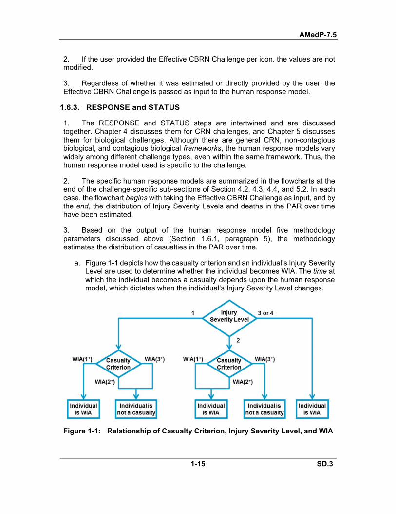
AMedP-7.5

1-15 SD.3

2. If the user provided the Effective CBRN Challenge per icon, the values are not modified.

3. Regardless of whether it was estimated or directly provided by the user, the Effective CBRN Challenge is passed as input to the human response model.

1.6.3. RESPONSE and STATUS

1. The RESPONSE and STATUS steps are intertwined and are discussed together. Chapter 4 discusses them for CRN challenges, and Chapter 5 discusses them for biological challenges. Although there are general CRN, non-contagious biological, and contagious biological frameworks, the human response models vary widely among different challenge types, even within the same framework. Thus, the human response model used is specific to the challenge.

2. The specific human response models are summarized in the flowcharts at the end of the challenge-specific sub-sections of Section 4.2, 4.3, 4.4, and 5.2. In each case, the flowchart begins with taking the Effective CBRN Challenge as input, and by the end, the distribution of Injury Severity Levels and deaths in the PAR over time have been estimated.

3. Based on the output of the human response model five methodology parameters discussed above (Section 1.6.1, paragraph 5), the methodology estimates the distribution of casualties in the PAR over time.

a. Figure 1-1 depicts how the casualty criterion and an individual’s Injury Severity Level are used to determine whether the individual becomes WIA. The time at which the individual becomes a casualty depends upon the human response model, which dictates when the individual’s Injury Severity Level changes.

Figure 1-1: Relationship of Casualty Criterion, Injury Severity Level, and WIA

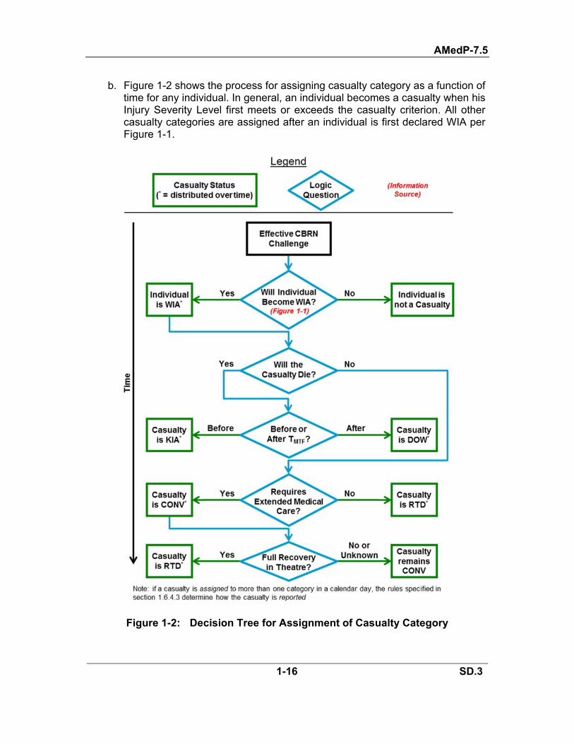
AMedP-7.5

1-16 SD.3

b. Figure 1-2 shows the process for assigning casualty category as a function of time for any individual. In general, an individual becomes a casualty when his Injury Severity Level first meets or exceeds the casualty criterion. All other casualty categories are assigned after an individual is first declared WIA per Figure 1-1.

Figure 1-2: Decision Tree for Assignment of Casualty Category

AMedP-7.5

1-17 SD.3

4. Composite Injury Profiles (for chemical and radiological agents) are the only means by which the methodology accounts for synergy between different injuries. Composite Injury Profiles are used to represent multiple challenge types from a single chemical or radiological agent (e.g., VX inhalation and percutaneous, or RDD cutaneous and whole body), but not of multiple chemical or radiological agents (e.g., VX and an RDD together).

1.6.4. REPORT

1. Per guidance from AJP-4.10, the four required outputs are labeled PAR, rates, flow, and profile. These provide an estimate of how many casualties occur, when they occur, the types of injury, and when changes in casualty category are expected to occur. An additional type of output, labeled “personnel status,” is also reported. Personnel status refers to the total number of casualties in a category on a certain day; this is contrasted to the rate, which only refers to new casualties.

a. The PAR is simply the total number of personnel included in the scenario—a user input.

b. Output tables

1) The rate table presents the number of new casualties in each category per day.39 It reports WIA without subdividing by Injury Severity Level. This form of output will be most useful for operational and personnel planners.

2) The personnel status table, which is not an AJP-4.10 requirement, reports the number of total casualties in each category on each day, with WIA subdivided by Injury Severity Level. Its purpose is to give an overall picture of the status of the force on each day. This form of output will be most useful for logistics and medical planners.

c. The flow characterizes the movement between casualty categories.40 The casualty flow is presented within the rate tables.

d. The profile is a description of the relative proportions of types of injuries. Some example injury types in the context of this document are “WIA—mild rad”, “CONV—GB,” and “KIA—C” (where C indicates “chemical”). The casualty profile is presented within the rate tables.

2. Reports are generated with a time resolution of one day; this is fixed.

39 AJP-4.10 also mentions the option to report a proportional rate. Although this is not included in the methodology, it can easily be calculated by the planner: simply multiply the actual rate by 100 and divide by the PAR. 40 AJP-4.10 also describes flow as characterizing how the timing of casualties depends on when incidents occur, which is beyond the purview of this document.

AMedP-7.5

1-18 SD.3

3. As it is possible for an individual to be assigned to multiple casualty categories within a single day, the rules in Table 1-4 are followed to facilitate more appropriate resource planning and to avoid double-counting.

Table 1-4: Casualty Reporting Rules Rule for Reporting the Value of # in WIA(#) for Personnel Status Tables

Initial Category, Day X Highest Severity, Day X Report As, Day X Report As, Day X+1

WIA(#) WIA(#+(1, 2, or 3)) WIA(#+(1, 2, or 3))* (no specific rule)

Rules for New Casualty and Personnel Status Tables

Initial Category, Day X Final Category, Day X Report As, Day X Report As, Day X+1 WIA KIA§ KIA KIA WIA DOW WIA† DOW WIA CONV WIA† CONV WIA RTD WIA† RTD

CONV RTD CONV RTD * In other words, for personnel status tables, always report the highest severity (value of #) that

occurred on that day. † For personnel status tables, the Injury Severity Level must also be included (e.g., WIA(2)). § By definition, this can only occur on day 1.

4. One point related to Table 1-4 warrants additional clarification. If, for example, an individual is RTD as of 72 hours (the end of Day 3 and start of Day 4), the individual should be reported as RTD on Day 4, because the individual ended Day 3 as RTD (at no point on Day 4 is the Injury Severity Level greater than zero). However, if the individual was RTD as of 73 hours, that individual would be reported as WIA on Day 4 and RTD on Day 5.

5. Reporting continues until no further changes in casualty category occur.

1.6.5. User Aids

1. Figure 1-3 provides a methodology overview.

AMedP-7.5

1-19 SD.3

Figure 1-3: AMedP-7.5(A) Methodology Overview

AMedP-7.5

1-20 SD.3

2. Table 1-5 is a roadmap for the user. For each agent, effect, or disease, it specifies the section of this document to be used to complete each of the five steps described above.

Table 1-5: User’s Roadmap

Agent, Effect, or Disease Five Steps

INPUT CHALLENGE RESPONSE/STATUS REPORT

Chemical GA Ch. 2 Ch. 3 Sections 4.2.2 and 4.1 Ch. 6 GB Ch. 2 Ch. 3 Sections 4.2.3 and 4.1 Ch. 6 GD Ch. 2 Ch. 3 Sections 4.2.4 and 4.1 Ch. 6 GF Ch. 2 Ch. 3 Sections 4.2.5 and 4.1 Ch. 6 VX Ch. 2 Ch. 3 Sections 4.2.6 and 4.1 Ch. 6 HD Ch. 2 Ch.3 and Section 4.2.7.3 Sections 4.2.7 and 4.1 Ch. 6 CG Ch. 2 Ch. 3 Sections 4.2.8 and 4.1 Ch. 6 Cl2 Ch. 2 Ch. 3 Sections 4.2.9 and 4.1 Ch. 6 NH3 Ch. 2 Ch. 3 Sections 4.2.10 and 4.1 Ch. 6 AC Ch. 2 Ch. 3 Sections 4.2.11 and 4.1 Ch. 6 CK Ch. 2 Ch. 3 Sections 4.2.12 and 4.1 Ch. 6 H2S Ch. 2 Ch. 3 Sections 4.2.13 and 4.1 Ch. 6

Radiological RDD Ch. 2 Ch. 3 and Section 4.3.2.3 Sections 4.3.2 and 4.1 Ch. 6

Fallout Ch. 2 Ch. 3 and Section 4.3.3.3 Sections 4.3.3 and 4.1 Ch. 6 Nuclear

Initial Whole-Body Radiation Ch. 2 Ch. 3 and Section 4.4.2.2 Sections 4.4.2 and 4.1 Ch. 6 Blast Ch. 2 Ch. 3 Sections 4.4.3 and 4.1 Ch. 6

Thermal Fluence Ch. 2 Section 4.4.4.2 Sections 4.4.4 and 4.1 Ch. 6 Biological

Anthrax Ch. 2 Ch. 3 Sections 5.2.1 and 5.1.4 Ch. 6 Brucellosis Ch. 2 Ch. 3 Sections 5.2.2 and 5.1.4 Ch. 6 Glanders Ch. 2 Ch. 3 Sections 5.2.3 and 5.1.4 Ch. 6

Melioidosis Ch. 2 Ch. 3 Sections 5.2.4 and 5.1.4 Ch. 6 Plague (non-contagious) Ch. 2 Ch. 3 Sections 5.2.5 and 5.1.4 Ch. 6

Plague (contagious) Ch. 2 Ch. 3 Sections 5.2.6 and 5.1.5 Ch. 6 Q Fever Ch. 2 Ch. 3 Sections 5.2.7 and 5.1.4 Ch. 6

Tularemia Ch. 2 Ch. 3 Sections 5.2.8 and 5.1.4 Ch. 6 Smallpox (non-contagious) Ch. 2 Ch. 3 Sections 5.2.9 and 5.1.4 Ch. 6

Smallpox (contagious) Ch. 2 Ch. 3 Sections 5.2.10 and 5.1.5 Ch. 6 EEEV disease Ch. 2 Ch. 3 Sections 5.2.11 and 5.1.4 Ch. 6 VEEV disease Ch. 2 Ch. 3 Sections 5.2.12 and 5.1.4 Ch. 6 WEEV disease Ch. 2 Ch. 3 Sections 5.2.13 and 5.1.4 Ch. 6

Botulism Ch. 2 Ch. 3 Sections 5.2.14 and 5.1.4 Ch. 6 Ricin Intoxication Ch. 2 Ch. 3 Sections 5.2.15 and 5.1.4 Ch. 6 SEB Intoxication Ch. 2 Ch. 3 Sections 5.2.16 and 5.1.4 Ch. 6

T-2 Mycotoxicosis Ch. 2 Ch. 3 Sections 5.2.17 and 5.1.4 Ch. 6

AMedP-7.5

1-21 SD.3

3. For additional information, Table 1-6 lists the cross-references between part(s) of this document and the corresponding part(s) of the SRD.

Table 1-6: Cross-References for AMedP-7.5 and Standards Related Document Topic AMedP-7.5 SRD

Definitions General Assumptions, Limitations, and Constraints

Chapter 1 Chapter 2

User Input; Default Parameter Values Chapter 2 Chapter 3 Calculation of Effective CBRN Challenge Chapter 3 N/A*

CRN Model Framework Section 4.1 Chapter 4 Chemical Agent Assumptions and Constraints Chemical Agent Toxicity Source Documents

Section 4.2.1 N/A† Chapter 5

Nerve Agent Models (GA, GB, GD, GF, and VX) Sections 4.2.2 to 4.2.6 Chapter 6 HD Model Section 4.2.7 Chapter 7 CG Model Section 4.2.8 Chapter 8Cl2 Model Section 4.2.9 Chapter 9 NH3 Model Section 4.2.10 Chapter 10 AC Model Section 4.2.11 Chapter 11 CK Model Section 4.2.12 Chapter 12 H2S Model Section 4.2.13 Chapter 13

Radiological Agent Assumptions and Limitations Nuclear Assumptions and Limitations Threshold Lethal Dose and Time to Death

Section 4.3.1 Section 4.4.1 Section 4.3.4

Chapter 14

RDD, Fallout, and Initial Whole-Body Radiation (Nuclear) Model

Section 4.3.2 Section 4.3.3 Section 4.3.5 Section 4.4.2

Chapter 15

Nuclear Blast Model Section 4.4.3 Chapter 16 Nuclear Thermal Fluence Model Section 4.4.4 Chapter 17

Biological Agent Model Framework Biological Agent Model Development Source Documents

Section 5.1 N/A†

Chapter 18

Anthrax Model Section 5.2.1 Chapter 19 Brucellosis Model Section 5.2.2 Chapter 20 Glanders Model Section 5.2.3 Chapter 21 Melioidosis Model Section 5.2.4 Chapter 22 Plague Model Sections 5.2.5 and 5.2.6 Chapter 23 Q Fever Model Section 5.2.7 Chapter 24 Tularemia Model Section 5.2.8 Chapter 25 Smallpox Model Sections 5.2.9 and 5.2.10 Chapter 26 EEEV Disease Model Section 5.2.11 Chapter 27 VEEV Disease Model Section 5.2.12 Chapter 28 WEEV Disease Model Section 5.2.13 Chapter 29 Botulism Model Section 5.2.14 Chapter 30 Ricin Intoxication Model Section 5.2.15 Chapter 31 SEB Intoxication Model Section 5.2.16 Chapter 32 T-2 Mycotoxicosis Model Section 5.2.17 Chapter 33

Casualty Summation and Reporting Chapter 6 N/A* * The SRD does not discuss this topic because the explanation in AMedP-7.5 was deemed sufficient. † AMedP-7.5 does not discuss this topic because it is not necessary for the execution of the

methodology; the topic is discussed in the SRD to provide supporting background information.

AMedP-7.5

1-22 SD.3

4. Table 1-7 provides some assistance with converting between different measurement units, because AMedP-7.5 uses units that may not be familiar to all readers.41 Familiarity with metric system units and prefixes is assumed. Note that for biological agents, the conversion between organisms and colony forming units (CFU) or virions and plaque forming units (PFU) is dependent upon too many factors to be standardized—no standard exists.

Table 1-7: Guide to AMedP-7.5 Measurement Units Quantity AMedP-7.5 Units Conversion to Other Common Units

Volume m3 1 m3 = 1000 L Mass kg, mg, µg 1 kg = 1000 mg = 106 µg = 2.2 lb Pressure kPa 101.325 kPa = 1 atm = 14.7 psi Energy kJ 4.184 kJ = 1 kcal = 1 Cal Breathing Rate m3/min 1 m3/min = 1000 L/min Radioactivity TBq 0.037 TBq = 1 Ci*

Equivalent Radiation Dose Sv 1 Sv = 100 rem*

Absorbed Radiation Dose Gy 1 Gy = 100 rad*

* “Ci” = Curie; “rem” = roentgen equivalent man; “rad” is not an abbreviation.

41 See https://en.wikipedia.org/wiki/Conversion_of_units for a comprehensive list of unit conversions.

AMedP-7.5

2-1 SD.3

CHAPTER 2 USER INPUT

This chapter fully describes each required and optional user input—it discusses the INPUT step of the methodology. It includes example input tables, default parameter values, and guidance to the user. A final aspect of user input, not discussed any further in this chapter, is that the user may edit any parameter value in the methodology. All given parameter values should be considered the default or recommended value, but users who wish to change values may do so. However, users must be cautious to use realistic parameter values, or odd results may occur.

2.1. ICONS AND ICON ATTRIBUTES

1. An icon is a group of individuals sharing a common location over time. For example, four people in a tank or a grouping of personnel in a fighting position. Each icon is assigned a unique numerical identifier called the icon index (n).

2. When defining icons, the user must determine the appropriate way to group individuals. For example, a cluster of individuals within a 10 km2 area may be represented by a single icon or by multiple icons. When considering scenarios covering several hundred square kilometers in area, users may wish to choose a lower spatial resolution—where each icon covers a larger geographic area—than when considering scenarios covering only a few square kilometers.

3. The user’s grouping of individuals into icons is external to the methodology. The input required by the methodology is described below in terms of icon attributes.

2.1.1. Overview of Icon Attributes

1. The user must provide the number of personnel in each icon.

2. The user may provide identifying information to assist in interpreting results, such as battalion, company, platoon, and area. This information is not used by the methodology.

3. The user must provide CBRN Challenge data (Input Scheme 1) or the Effective CBRN Challenge (Input Scheme 2). These inputs must be derived from the user's national hazard prediction model, which is separate from AMedP-7.5.

4. If the user provides CBRN Challenge (Input Scheme 1), then it is strongly recommended that the user also define challenge-modifying attributes to match the planning scenario; otherwise, default values will be used. Table 2-1 summarizes the attributes, including default values, and identifies which attributes are considered when estimating an icon’s Effective CBRN Challenge, as a function of the challenge type. The values of challenge-modifying icon attributes may change over time, as specified by the user.

AMedP-7.5

2-2 SD.3

Table 2-1: Challenge-Modifying Icon Attributes

Challenge Type Attributes and Potential Methodological Relevance

Breathing Rate

Body Surface Area

IPE Vehicle or

Shelter* Pre-exposure Prophylaxis

Uniform

Chemical inhalation X X X X Chemical perc. vapour X X X Chemical perc. liquid X X X X Biological inhalation X X X †

Gamma radiation X‡ X‡ X Neutron radiation X‡ X‡ X

Beta radiation X‡ X¥ X Blast (nuclear) X

Thermal (nuclear) X X Default Values for All Challenge Types§

0.015 m3/min

0.9 m2 None None None Battledress

Uniform (BDU) + T-shirt

* Relates to physical protection and ColPro. † Note that prophylaxis for biological agents is accounted for separately; see Section 5.1. § Used if the user does not specify alternate values. ‡ Only used for calculating inhaled dose. ¥ Used for both inhaled dose and cutaneous dose calculations.

5. If the user provides the Effective CBRN Challenge (Input Scheme 2), then the methodology will not use the challenge-modifying attributes.

6. The use of icons and icon attributes supports several important features.

a. Using icons supports the application of spatially resolved output from national hazard prediction models, despite icon location not being an input for this methodology.

b. Using icon attributes allows the user to account for a postulated distribution of defensive postures across the PAR.

c. The ability to change the values of icon attributes over time allows the user to account for warning and response, which is the combined process of gathering information indicating that a CBRN incident has occurred, assessing that information to determine its meaning and implications, and deciding upon an appropriate tactical response. Examples of tactical responses the icon attributes might account for are:

1) A command decision that all personnel must wear certain IPE because of the assessed threat.

2) Donning IPE or taking shelter in response to observing nerve agent poisoning symptoms in some personnel.

3) Donning IPE or taking shelter in response to a detector alarm.

AMedP-7.5

2-3 SD.3

2.1.2. CBRN Challenge or Effective CBRN Challenge

1. The user may supply CBRN Challenge information via one of two input schemes (summarized in the INPUT box in Figure 1-3). The choice of input scheme should be determined by whether the user is able to provide input for the challenge-modifying icon attributes. As more input is provided, the resulting casualty estimate will better match the planning scenario. For either input scheme, the CBRN challenge data must be generated using national tools—there is no NATO standardized method of generating CBRN challenge estimates (ATP-4542 predicts hazard areas, but not hazard magnitudes).

2. CBRN Challenge (Input Scheme 1).

a. The user must provide data for each icon at each time point. Note, however, that if desired, a user may choose to provide data at only one time point (the end of the challenge).

b. The final time point should be the time past which the CBRN Challenge no longer increases—that is, the provided input should encompass the entire period over which icons are challenged.

c. Time must be specified in units of minutes. The total duration, number of time points, and intervals between time points are user-specified. A varying time interval is allowed, but the time intervals must be the same for all icons. Likewise, “time zero” must be the same for all icons.

d. The user should ensure that the national tool used to generate the challenge data has time resolution sufficient to capture the fidelity of icon movement43 and defensive action the user desires to model. For example, if the user wishes to capture the ability of individuals to don a mask in 15 seconds, the time interval around the time when individuals don masks should be 15 seconds (0.25 minutes) or shorter. If icons are not moving or taking any defensive actions and the hazard changes slowly, a time interval of up to 5 minutes is acceptable. If the user is unsure of what time resolution to use, 1 minute is a reasonable default.

e. For all challenge types other than chemical agent peak concentration, the data must be cumulative, not instantaneous. Cumulative relates to the area under the curve of a plot of challenge versus time, whereas instantaneous relates to the specific magnitude of the challenge at a given time. If the user’s national hazard prediction model only outputs instantaneous data, the user must use a numerical integration technique44 to generate the cumulative input data

42 NATO, ATP-45(E). 43 Note that although the methodology does not use icon locations, icon movement could be reflected by changes in the values of challenge-modifying icon attributes. 44 For example, Simpson’s rule (see http://en.wikipedia.org/wiki/Simpson%27s_rule).

AMedP-7.5

2-4 SD.3

required by the methodology. As specified in Section 1.4.3.b., chemical agent peak concentration challenge data should be instantaneous.

3. Effective CBRN Challenge (Input Scheme 2).

a. The user must provide a single value for each icon.

b. The methodology will not modify the user-provided values. Thus, the user must already have accounted for the challenge-modifying icon attributes.

4. The input must be provided in the units specified in Table 2-2. If Input Scheme 1 is used, the methodology will calculate the Effective CBRN Challenge in the appropriate units.

Table 2-2: Challenge Types and Associated Units for CBRN Challenges Agent or Effect Challenge Type

(Subcomponents, if any) Symbol (Q)

CBRN Challenge

(Input Scheme 1)

Effective CBRN Challenge

(Input Scheme 2)

GA Inhaled GA

GA,ih

mg-min/m3

mg-min/m3

GB Inhaled GB

GB,ih

mg-min/m3

mg-min/m3

GD Inhaled GD

GD,ih

mg-min/m3

mg-min/m3

GF Inhaled GF

GF,ih

mg-min/m3

mg-min/m3

VX Inhaled VX Percutaneous VX Liquid

VX,ih

VX,pc

mg-min/m3

mg/m2

mg-min/m3

mg HD

Inhaled HD Ocular HD

(Percutaneous Vapour) Equivalent Percutaneous HD

(Percutaneous Vapour) (Percutaneous Liquid)

HD,ih HD,oc HD,pv

HD,epc HD,pv HD,pl

mg-min/m3

mg-min/m3

mg-min/m3

mg/m2

mg-min/m3 mg-min/m3

mg-min/m3

CG Inhaled CG Peak CG Concentration

CG,ih CG,[ih]

mg-min/m3

mg/m3

mg-min/m3

mg/m3 Cl2

Inhaled Cl2

Cl2,ih

mg-min/m3

mg-min/m3

NH3

Inhaled NH3

NH3,ih

mg-min/m3

mg-min/m3

AC Inhaled AC

AC,ih

mg-min/m3

mg-min/m3

CK Inhaled CK Peak CK Concentration

CK,ih CK,[ih]

mg-min/m3

mg/m3

mg-min/m3

mg/m3

H2S Inhaled H2S

H2S,ih

mg-min/m3

mg-min/m3

AMedP-7.5

2-5 SD.3

Agent or Effect Challenge Type

(Subcomponents, if any) Symbol (Q)

CBRN Challenge

(Input Scheme 1)

Effective CBRN Challenge

(Input Scheme 2) RDD

Cutaneous Radiation (Skin Contamination) (Cloudshine) (Groundshine)

Whole-Body Radiation (Cloudshine) (Groundshine) (Inhalation)

RDD,cut

RDD,cut,s RDD,cut,cld RDD,cut,grd

RDD,wb RDD,wb,cld RDD,wb,grd RDD,wb,ih

TBq/m2

TBq-hr/m3

TBq-hr/m2

TBq-hr/m3 TBq-hr/m2

TBq-min/m3

Gy

Gy

Fallout Cutaneous Radiation

(Skin Contamination) (Groundshine Gamma) (Groundshine Beta)

Whole-Body Radiation (Groundshine)

FO,cut

FO,cut,s FO,cut,grd-γ FO,cut,grd-β

FO,wb FO,wb,grd

TBq-hr/m2

Gy Gy

Gy

Gy

Gy

Nuclear Detonation Whole-Body Radiation

(Neutron) (Gamma)

Blast Static Overpressure Thermal Fluence

nuc,wb

nuc,wb,n0 nuc,wb,γ nuc,blast

nuc,thermal

Gy Gy kPa

kJ/m2

Gy

kPa %BSA

Anthrax Inhaled B. anthracis

anth

spore-min/m3

spore

Brucellosis Inhaled Brucella

bruc

CFU-min/m3

CFU

Glanders Inhaled B. mallei

glan

CFU-min/m3

CFU

Melioidosis Inhaled B. pseudomallei

meli

CFU-min/m3

CFU

Plague Inhaled Y. pestis

plag

CFU-min/m3

CFU

Q fever Inhaled C. burnetii

Qfvr

organism-min/m3

organism

Tularemia Inhaled F. tularensis

tul

organism-min/m3

organism

Smallpox Inhaled V. major

spox

PFU-min/m3

PFU

EEEV Disease Inhaled EEEV

EEEVD

PFU-min/m3

PFU

VEEV Disease Inhaled VEEV

VEEVD

PFU-min/m3

PFU

WEEV Disease Inhaled WEEV

WEEVD

PFU-min/m3

PFU

Botulism Inhaled Botulinum neurotoxin

bot

µg-min/m3

µg

Ricin Inhaled Ricin

ricin

µg-min/m3

µg

Staphylococcal enterotoxin B (SEB) Inhaled SEB

SEB

µg-min/m3

µg

T-2 Mycotoxin Inhaled T-2 Mycotoxin

T-2

mg-min/m3

mg

Note: for assistance converting measurement units, see Table 1-7.

AMedP-7.5

2-6 SD.3

2.1.3. Breathing Rate

1. For inhaled chemical agent, inhaled biological agent, and inhaled radiological particle (contributes to whole-body dose for RDD) challenges, the breathing rate is used in the calculation of the inhaled45 concentration time (chemical), dose (biological), or dose equivalent (radiological particles).

2. The user may specify either the qualitative level of activity—which will be converted to a breathing rate according to Table 2-3—or a specific breathing rate in units of m3/min. If no input is provided, the default values in Table 2-3 will be used.

3. The chemical agent human response models have a built-in assumption of a 0.015 m3/min (15 L/min) breathing rate. Thus, breathing rate is not used directly; a unitless factor defined as the breathing rate divided by 0.015 m3/min is used.

4. The biological agent and RDD human response models do not have a built-in breathing rate assumption, so breathing rate in units of m3/min is used.

5. Table 2-3 specifies the default and suggested alternate values for the breathing rate. The user may specify any desired breathing rate.

Table 2-3: Suggested and Default Breathing Rates Optional Input—user need specify only one, or may use defaults

Challenge Type Activity Level Breathing Rate [m3/min*]† Unitless Factor§

Chemical Agent Inhalation

At Rest 0.0075 0.5 Light (default) 0.0150 (default) 1 (default)

Moderate 0.0300 2

Heavy 0.0750 5

Biological Agent and Radiological Particle

Inhalation

At Rest 0.0075 N/A Light (default) 0.0150 (default) N/A

Moderate 0.0300 N/A

Heavy 0.0750 N/A * Multiply breathing rate in m3/min by 1000 to convert to L/min. † Derived from David W. Layton, “Metabolically Consistent Breathing Rates for Use in Dose

Assessments,” Health Physics 64, no. 1 (1993): 23–36. § The unitless factor is calculated by dividing the actual breathing rate by 0.015 m3/min.

2.1.4. Body Surface Area

1. For liquid chemical agent challenges, the total body surface area challenged is used in the calculation of the dose.

2. The standard man is typically assumed to have 1.8 m2 of body surface area. As most hazard prediction models do not have the fidelity to determine the orientation of

45 The fraction of inhaled agent that is retained is irrelevant because the underlying models are based on the amount of inhaled agent

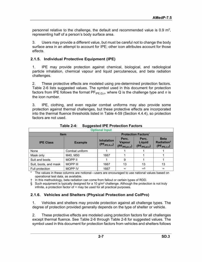
AMedP-7.5

2-7 SD.3

personnel relative to the challenge, the default and recommended value is 0.9 m2, representing half of a person’s body surface area.

3. Users may provide a different value, but must be careful not to change the body surface area in an attempt to account for IPE; other icon attributes account for those effects.

2.1.5. Individual Protective Equipment (IPE)

1. IPE may provide protection against chemical, biological, and radiological particle inhalation, chemical vapour and liquid percutaneous, and beta radiation challenges.

2. These protective effects are modeled using pre-determined protection factors. Table 2-6 lists suggested values. The symbol used in this document for protection factors from IPE follows the format PFIPE,Q,n, where Q is the challenge type and n is the icon number.

3. IPE, clothing, and even regular combat uniforms may also provide some protection against thermal challenges, but these protective effects are incorporated into the thermal fluence thresholds listed in Table 4-59 (Section 4.4.4), so protection factors are not used.

Table 2-4: Suggested IPE Protection Factors Optional Input

Item Protection Factors*

IPE Class Example Inhalation (PFIPE,ih,n)

Perc. Vapour

(PFIPE,pv,n)

Perc. Liquid

(PFIPE,pl,n)

Beta Radiation† (PFIPE,β,n)

None Combat uniform 1 1 1 1 Mask only M40, M50 1667 1 1 1

Suit and boots MOPP II 1 9 1 1

Suit, boots, and mask MOPP III 1667 13 13 13

Full protection MOPP IV 1667 ∞ ∞§ ∞ * The values in these columns are notional—users are encouraged to use national values based on

operational test data, as available. † In this methodology, beta radiation can come from fallout or certain types of RDD. § Such equipment is typically designed for a 10 g/m2 challenge. Although the protection is not truly

infinite, a protection factor of ∞ may be used for all practical purposes.

2.1.6. Vehicles and Shelters (Physical Protection and ColPro)

1. Vehicles and shelters may provide protection against all challenge types. The degree of protection provided generally depends on the type of shelter or vehicle.

2. These protective effects are modeled using protection factors for all challenges except thermal fluence. See Table 2-6 through Table 2-8 for suggested values. The symbol used in this document for protection factors from vehicles and shelters follows

AMedP-7.5

2-8 SD.3

the format PFV-SH,Q,n.

a. Vehicles and shelters are assumed to completely protect icons from liquid chemical agent challenges.

b. Inhalation and percutaneous vapour protection afforded by vehicles and shelters with ColPro is modeled using pre-determined protection factors.

c. Inhalation and percutaneous vapour protection afforded by vehicles and shelters without ColPro is modeled using protection factors that must be estimated on a per-icon and per-challenge basis using Equation 2-1, which depends upon the air exchange rate, the duration of occupancy, and the duration the vehicle or shelter is enveloped in the cloud.46 The maximum calculated PF occurs when Occupancyn = Durationn, and the PF decreases as Occupancyn increases beyond Durationn.

PFV-SH,ih/pv,n=AERn·Durationn

AERn·Durationn+e(-AERn·Occupancyn)-eAERn·(Durationn-Occupancyn) , (2-1)

where:

PFV-SH,ih/pv,n is the protection factor for icon n for the duration of Occupancyn,

AERn is the air exchange rate at icon n [air changes per hour (ACH)]—Table 2-5 provides suggested air exchange rates for various vehicles and shelters,

Durationn is the length of time the cloud envelopes the vehicle/structure while it is occupied by icon n [hr], and

Occupancyn is the length of time of vehicle/structure occupancy from the time of cloud arrival at icon n [hr], which must be greater than or equal to Durationn.

Note for Input Scheme 1: if an icon leaves the vehicle or shelter while it is still enveloped, Durationn and Occupancyn must be set equal to avoid negative numbers. Accordingly, the resulting protection factor must only be applied to the time steps during which the icon occupied the vehicle or shelter.

46 William K. Blewett et al., Expedient Sheltering in Place: An Evaluation for the Chemical Stockpile Emergency Preparedness Program (Aberdeen Proving Ground, MD: Edgewood Research Development and Engineering Center, June 1996), 14–20.

AMedP-7.5

2-9 SD.3

Table 2-5: Suggested Air Exchange Rates for Vehicles and Shelters Without ColPro

Optional Input

Vehicle or Shelter Ventilation Class Examples AERn

*

[ACH]

Residential Building – Closed Windows Barracks 0.5 Nonresidential Building – Closed Windows

Administrative, Control and Work Buildings

1.3

Residential Building – Open Windows Hangar 6.4

Stationary Vehicle – Open Windows, No Ventilation

Chem-Bio Protective System (CBPS), Tent†, Tactical Operations Center (TOC)

20

Stationary Vehicle – Closed Windows, Fan on Recirculation

Self-Propelled Howitzer, Truck/Van, Recovery

2.5

Stationary Vehicle – Closed Windows, No Ventilation

2

Moving Vehicle – Closed Windows Armored Engineer Vehicle (AEV), Armored Personnel Carrier (APC)

36

Stationary Vehicle – Open Windows, Fan on Fresh Air

Truck/Van 40

* Adapted from J. H. Park et al., “Measurement of Air Exchange Rate of Stationary Vehicles and Estimation of in-Vehicle Exposure,” Journal of Exposure Analysis and Environmental Epidemiology 8, no. 1 (1998): 65–78 and Ted Johnson, A Guide to Selected Algorithms, Distributions, and Databases Used in Exposure Models Developed by the Office of Air Quality Planning and Standards (Chapel Hill, NC: TRJ Environmental, Inc., 2002).

† Tents are assumed to have an ACH of 20, the same as a stationary vehicle with windows open and no ventilation.

Table 2-6: Suggested Inhalation and Percutaneous Protection Factors for Vehicles and Shelters

Optional Input

Vehicle or Shelter Ventilation Class

Example Inhalation(PFV-SH,ih,n)

Perc. Vapour (PFV-SH,pv,n)

Perc. Liquid(PFV-SH,pl,n)

None Dismounted, Foxhole 1 1 1

Vehicle w/ColPro CBPS, TOC, Recovery, Self-Propelled Howitzer, AEV, APC

3000 3000 ∞

Vehicle w/o ColPro Mortar, Mobile Surface-to-Air Missile Launcher, Tent, Truck/Van

Use Equation 2-1 ∞

Shelter w/ColPro Admin Building, Control Building, ColPro Barracks

3000 3000 ∞

Shelter w/o ColPro Barracks, Hangar, Work Building Use Equation 2-1 ∞ * The values in these columns are notional—users are encouraged to use national values based on

operational test data, as available.

d. Radiation and blast shielding afforded by vehicles and shelters are modeled using pre-determined protection factors. Suggested protection factors are listed in Table 2-7 and Table 2-8. Note that the level of protection each vehicle or shelter provides is typically different for neutron and gamma radiation. Further, all vehicles and shelters are assumed to provide complete protection from beta radiation, so the suggested protection factor is ∞. Finally, the

AMedP-7.5

2-10 SD.3

inhalation protection provided against radiological particles should be based on the previous discussion of inhalation protection.

Table 2-7: Suggested Radiation Shielding Protection Factors for Vehicles and Shelters

Optional Input

Vehicle or Shelter Radiation Class

Neutron Radiation (PFV-SH,n0,n)

Gamma Radiation (PFV-SH,γ,n)

Armored Personnel Carrier 1.22 2.70 Earth Shelter 16.67 66.67

Exposed/Dismounted 1.00 1.00

Foxhole (nuclear only)† 3.00 10.00

Masonry Building 8.33 6.67

Multi-Story Brick Building 1.33 1.56

Tank 3.57 10.00

Tent 1.00 1.00

Truck 1.00 1.25

Van 1.05 1.05

Wood Frame Building 1.39 1.22 * The values in this table are notional—users are encouraged to use other values based on

operational test data, as available. † For RDD and fallout challenges, foxholes should be modeled with protection factors of 1.

Table 2-8: Suggested Blast Shielding Protection Factors Optional Input

Vehicle/Shelter Blast Class Blast Shielding Protection Factor* (PFV-SH,blast,n)

All 1 * No generally accepted blast shielding protection factors were available; this table is a placeholder.

Users may input specific national data, if desired.

3. The protection vehicles and shelters provide from thermal fluence is not modeled using protection factors because the equation used to estimate thermal insults is not applicable to partially protected bodies. For details on how it is included in the human response estimates, see Section 4.4.4.

2.1.7. Pre-Exposure Prophylaxis

1. In general, pre-exposure prophylaxis might provide protection against any challenge type.

2. No currently fielded prophylaxis options are modeled using protection factors, so Table 2-9 is a placeholder to help illustrate how the methodology would incorporate prophylaxis, pending future development of relevant prophylaxis. The symbol used in this document for protection factors from pre-exposure prophylaxis follows the format PFproph,Q,n, where Q is the challenge type.

AMedP-7.5

2-11 SD.3

Table 2-9: Suggested Protection Factors for CRN Prophylaxis Optional Input

Specific Prophylaxis Challenge Type(s) For Which the Prophylaxis is Effective

Prophylaxis Protection Factor* (PFproph,Q,n)

None All 1 * No relevant prophylaxis is currently fielded; this table is a placeholder for future capabilities. Users

may input specific national data, if desired.

3. Note that although vaccination and/or chemoprophylaxis are available for many biological agents, the protective effects are not modeled using a protection factor—see Section 5.2 for details on how each biological agent prophylaxis option is used in the human response estimate.

2.1.8. Uniform

Uniforms may provide some protection against thermal challenges, but these protective effects are incorporated into the thermal fluence thresholds listed in Table 4-59 (Section 4.4.4), so protection factors are not used.

2.1.9. Aggregate Protection Factor

1. The protection factors associated with the IPE, vehicle or shelter, and pre-exposure prophylaxis attributes are used in Equation 2-2 to calculate an icon’s Aggregate Protection Factor (APF), which is used in the equations in Chapter 3 during the calculation of an icon’s Effective CBRN Challenge.

APFQ,n = PFIPE,Q,n · PFV-SH,Q,n · PFproph,Q,n, (2-2)

where:

APFQ,n is icon n’s APF for challenge type Q,

PFIPE,Q,n is the protection factor for challenge type Q from all IPE used by icon n,

PFV-SH,Q,n is the protection factor for challenge type Q from the vehicle or shelter occupied by icon n (accounts for physical protection and ColPro), and

PFproph,Q,n is the protection factor for challenge type Q from any pre-exposure prophylaxis used by icon n.

2. If the user does not provide input for a particular protection factor, the default value of 1 is used. Thus, if the user provides no input for any protection factor, the APF = 1—no protection is modeled.

2.1.10. Example Input and Comparison of Input Schemes

1. Table 2-10 is an example of icon definitions including identifying information.

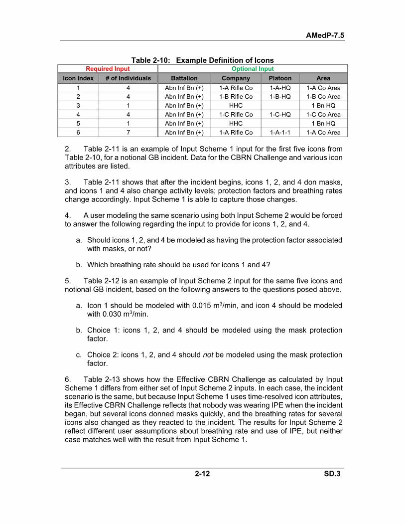
AMedP-7.5

2-12 SD.3

Table 2-10: Example Definition of Icons Required Input Optional Input

Icon Index # of Individuals Battalion Company Platoon Area

1 4 Abn Inf Bn (+) 1-A Rifle Co 1-A-HQ 1-A Co Area 2 4 Abn Inf Bn (+) 1-B Rifle Co 1-B-HQ 1-B Co Area

3 1 Abn Inf Bn (+) HHC 1 Bn HQ

4 4 Abn Inf Bn (+) 1-C Rifle Co 1-C-HQ 1-C Co Area

5 1 Abn Inf Bn (+) HHC 1 Bn HQ

6 7 Abn Inf Bn (+) 1-A Rifle Co 1-A-1-1 1-A Co Area

2. Table 2-11 is an example of Input Scheme 1 input for the first five icons from Table 2-10, for a notional GB incident. Data for the CBRN Challenge and various icon attributes are listed.

3. Table 2-11 shows that after the incident begins, icons 1, 2, and 4 don masks, and icons 1 and 4 also change activity levels; protection factors and breathing rates change accordingly. Input Scheme 1 is able to capture those changes.

4. A user modeling the same scenario using both Input Scheme 2 would be forced to answer the following regarding the input to provide for icons 1, 2, and 4.

a. Should icons 1, 2, and 4 be modeled as having the protection factor associated with masks, or not?

b. Which breathing rate should be used for icons 1 and 4?

5. Table 2-12 is an example of Input Scheme 2 input for the same five icons and notional GB incident, based on the following answers to the questions posed above.

a. Icon 1 should be modeled with 0.015 m3/min, and icon 4 should be modeled with 0.030 m3/min.

b. Choice 1: icons 1, 2, and 4 should be modeled using the mask protection factor.

c. Choice 2: icons 1, 2, and 4 should not be modeled using the mask protection factor.

6. Table 2-13 shows how the Effective CBRN Challenge as calculated by Input Scheme 1 differs from either set of Input Scheme 2 inputs. In each case, the incident scenario is the same, but because Input Scheme 1 uses time-resolved icon attributes, its Effective CBRN Challenge reflects that nobody was wearing IPE when the incident began, but several icons donned masks quickly, and the breathing rates for several icons also changed as they reacted to the incident. The results for Input Scheme 2 reflect different user assumptions about breathing rate and use of IPE, but neither case matches well with the result from Input Scheme 1.

AMedP-7.5

2-13 SD.3

7. Even without the details of how the Effective CBRN Challenge is used to estimate casualties, it is clear from Table 2-13 that three different ways of representing the same incident scenario can result in different casualty estimates.47 In general, Input Scheme 1 better reflects operational reality—personnel will react to a CBRN incident; the user should use Input Scheme 1 whenever possible.

Table 2-11: Example Input for Input Scheme 1, for a Notional GB Incident Required Input Optional Input

Icon Index

Time (min)

Concentration-time (mg-min/m3)

Activity Level*

IPE Class† Vehicle or Shelter Class†

Prophylaxis†

1 0 0 At Rest None None None 1 1 15.0 Moderate Mask None None

1 4 38.4 Light Mask None None

1 8 52.0 Light Mask None None

1 10 55.0 Light Mask None None

2 0 0 Light None None None 2 1 60.2 Light Mask None None

2 4 192.8 Light Mask None None

2 8 312.0 Light Mask None None

2 10 345.4 Light Mask None None

3 0 0 At Rest None Shelter w/ColPro None 3 1 0 At Rest None Shelter w/ColPro None

3 4 0 At Rest None Shelter w/ColPro None

3 8 0 At Rest None Shelter w/ColPro None

3 10 0 At Rest None Shelter w/ColPro None

4 0 0 At Rest None None None 4 1 18.8 Moderate None None None

4 4 23.8 Heavy Mask None None

4 8 23.8 Heavy Mask None None

4 10 23.8 Heavy Mask None None

5 0 0 At Rest None Shelter w/ColPro None 5 1 0 At Rest None Shelter w/ColPro None

5 4 7.8 At Rest None Shelter w/ColPro None

5 8 35.0 At Rest None Shelter w/ColPro None

5 10 42.8 At Rest None Shelter w/ColPro None * Instead of activity level, a user could provide a specific breathing rate—see Table 2-3. † Instead of these general descriptors, a user could provide a specific protection factor for each icon

attribute (see Table 2-4 through Table 2-9).

47 For the curious reader, the best example of the difference is icon 4: under Input Scheme 1, icon 4 would become WIA and eventually RTD; under Input Scheme 2 (Choice 1), icon 4 would not become casualties; under Input Scheme 2 (Choice 2), icon 4 would become KIA if untreated, or WIA and eventually permanently CONV if treated.

AMedP-7.5

2-14 SD.3

Table 2-12: Example Input for Input Scheme 2, for a Notional GB Incident Required Input

Icon Index Inhaled Concentration Time (mg-min/m3)

Choice 1 Choice 2 1 0.03 55.00 2 0.21 345.40

3 0.00 0.00

4 0.03 47.60

5 0.01 0.01

Table 2-13: Example Differences in Effective CBRN Challenge Resulting from Using Different Input Schemes for the Same Notional GB Incident

Input Scheme 1 Input Scheme 2—Choice 1 Input Scheme 2—Choice 2

Icon Index

Inhaled Concentration Time (mg-min/m3)

Inhaled Concentration Time (mg-min/m3)

Inhaled Concentration Time (mg-min/m3)

1 7.54 0.03 55.00 2 60.4 0.21 345.40

3 0.00 0.00 0.00

4 9.41 0.03 47.60

5 0.01 0.01 0.01

2.2 METHODOLOGY PARAMETERS

1. For each parameter below, the user may specify a value. If no value is specified, the default defined in Table 2-14 will be used.

2. Medical Treatment Flag (FlagMT). A binary parameter that determines whether the effects of medical treatment are modeled. If set to NO, the “Untreated” models are used; in general, these models reflect no medical treatment.48 If set to YES, the “Treated” human response models are used; these models are intended to reflect all available medical treatment. The default value is YES.

3. Time at Injury Severity Level 4 sufficient to cause death from untreated chemical, nuclear blast, or nuclear burn injuries (Tdeath-CN-SL4). Untreated49 casualties with a chemical, nuclear blast, or nuclear burn injury that spend this amount of time at Severity Level 4 are assumed to die. The default value is 15 minutes.

a. When FlagMT = Yes (the default value), all such casualties are KIA, because once a casualty reaches a MTF, medical treatment models are used to determine the outcome.

48 Models derived from animal data truly reflect no medical treatment. However, some of the biological agent models are derived from human data and include the effects of supportive care. 49 Including not yet treated casualties en route to a MTF.

AMedP-7.5

2-15 SD.3

b. When FlagMT = No, all casualties follow this assumption, even after reaching a MTF. Thus, KIA and DOW casualties may be a result of extended periods of Injury Severity Level 4.

4. Time to reach a medical treatment facility (TMTF). The time required for an individual who is WIA to reach a MTF. Given the definitions of KIA and DOW, TMTF determines whether a WIA who dies is KIA or DOW (see Figure 1-2). The default value is 30 minutes, and a user can specify any value up to (but excluding) 1 day—the methodology is built around the assumption that casualties reach an MTF within one day of becoming WIA.

5. The casualty criterion. The user-specifiable injury severity threshold above which an individual is declared WIA. The user may choose between WIA(1+), WIA(2+), and WIA(3+). WIA(1+) will typically result in individuals being declared casualties and then reporting to the medical system sooner than would WIA(2+) or WIA(3+) (see Figure 1-1). Methodologically, reporting to the medical system for injuries of lower severity results in fewer deaths and more personnel in the medical system (individuals are less likely to die before reaching an MTF). The default value is WIA(1+).

6. The day on which antibiotic or antitoxin treatment begins (dtrt-Q). For some bacterial diseases and for botulism, an individual’s prognosis and/or duration of illness depend upon when treatment with antibiotic or antitoxin begins. The methodology default value is day 1, which is likely to be optimistic. It is recommended that the user specify values based the following considerations, three of which are operation-specific.

a. The difficulty of differential diagnosis of the disease in the absence of specific intelligence information.

b. Anticipated intelligence regarding enemy capabilities and intentions, which might raise a doctor’s index of suspicion, facilitating quicker diagnosis.

c. Anticipated real-time or near-real-time detection of the attack.

d. Logistics delays, if a specialized treatment is required but not stocked locally.

Table 2-14: Default Values for User-Specifiable Parameters Parameter Default

Time to Reach a Medical Treatment Facility (TMTF) 30 minutes Time at Severity Level 4 Sufficient to Cause Death From Chemical,

Nuclear Blast, or Nuclear Burn Injuries (Tdeath-CN-SL4) 15 minutes

Medical Treatment Flag (FlagMT) Yes

Casualty Criterion WIA(1+)

The day on which antibiotic or antitoxin treatment begins (dtrt-Q) Day 1

INTENTIONALLY BLANK

AMedP-7.5

3-1 SD.3

CHAPTER 3 EFFECTIVE CBRN CHALLENGE ESTIMATION

This chapter provides the general framework for calculating the Effective CBRN Challenge from the inputs described in Chapter 2—it discusses the CHALLENGE step of the methodology. Special considerations for certain challenge types are fully described in Chapter 4, Sections 4.2 through 4.4. The CBRN Challenge inputs needed for the equations in this chapter (XQ,n,tk) must be derived from the user’s national hazard prediction model.

3.1. INPUT SCHEME 1

1. For each challenge type other than inhaled chemical agent peak concentration, each icon’s Effective CBRN Challenge is estimated using Equation 3-1, which incrementally sums (over time) the portion of the CBRN Challenge that becomes the Effective CBRN Challenge. The difference term in parentheses calculates the incremental CBRN Challenge during the timestep from tk to tk-1, and Z and APFQ,n,tk-1

convert the incremental CBRN Challenge into the incremental Effective CBRN Challenge. See Table 2-11 for an example of input that could be used with Equation 3-1.

XQ,neff =

(XQ,n,tk - XQ,n,tk-1) · Z

APFQ,n,tk-1

f

k = 1

, (3-1)

where:

XQ,neff is the Effective CBRN Challenge for challenge type Q and icon n,

tk is the time variable,

t0 is the first time point with non-zero CBRN Challenge,

tf is the time at which the CBRN Challenge ends,

XQ,n,tk is the CBRN Challenge for challenge type Q and icon n at time tk (derived from the output of the user’s national hazard prediction model),

APFn,tk-1 is the Aggregate Protection Factor for icon n for time tk‐1≤ t < tk, and

Z is a special factor whose value depends upon the context, per the following list:

a. For an inhaled chemical agent challenge, Z is the unitless factor described in Table 2-3 (related to the breathing rate icon attribute). The

AMedP-7.5

3-2 SD.3

value can vary by time step and icon, so Z becomes Zn,tk-1.

b. For an inhaled biological agent challenge, Z is the breathing rate icon attribute [m3/min]. Table 2-3 lists default and suggested values. The value can vary by time step and icon, so Z becomes Zn,tk-1

.

c. For a percutaneous liquid chemical agent challenge, Z is the body surface area icon attribute [m2]. The default value is 1 m2, and Section 2.1.4 contains user guidance relating to changing the value.

d. For RDD challenges other than inhalation, Z is a dose conversion factor—it is used to convert from units of radioactivity (TBq) to units of absorbed dose (gray). Dose conversion factors do not vary with time or by icon, but they are isotope-specific and have different values for cloudshine, groundshine, skin contamination, and inhalation. Table 3-1 provides default values.

e. For RDD inhalation challenge, Z is the mathematical product of the dose conversion factor for inhalation, default values of which are given in Table 3-1, and the breathing rate icon attribute [m3/min]. Table 2-3 lists default and suggested values for the breathing rate. As breathing rate can vary by time step and icon, Z becomes Zn,tk-1

.

f. For a fallout groundshine challenge, Z is a gamma-to-beta dose conversion factor—it is used to calculate the beta radiation dose based on the gamma radiation dose. Table 3-2 provides default values.

g. For a fallout skin contamination challenge, Z is a dose conversion factor—it is used to convert from units of radioactivity (TBq per area) to units of absorbed dose rate (gray per hour). The dose conversion factor does not vary by icon, and its variance with time is sufficiently slow and low-magnitude that it can be ignored. Table 3-2 provides default values.

h. For nuclear challenges, Z is not needed, so its value is 1.

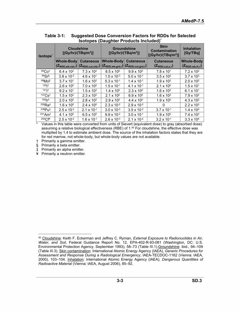
AMedP-7.5

3-3 SD.3

Table 3-1: Suggested Dose Conversion Factors for RDDs for Selected Isotopes (Daughter Products Included)*

Isotope*

Cloudshine [(Gy/hr)/(TBq/m3)]

Groundshine [(Gy/hr)/(TBq/m2)]

Skin Contamination

[(Gy/hr)/(TBq/m2)]

Inhalation [Gy/TBq]

Whole-Body (ZRDD,wb,cld,r)

Cutaneous (ZRDD,cut,cld,r)

Whole-Body (ZRDD,wb,grd,r)

Cutaneous (ZRDD,cut,grd,r)

Cutaneous (ZRDD,cut,s,r)

Whole-Body(ZRDD,wb,ih,r)

60Co† 6.4 x 102 7.3 x 102 8.5 x 100 9.9 x 100 7.8 x 101 7.2 x 102 90Sr§ 3.8 x 10-2 4.6 x 101 1.0 x 10-3 5.0 x 10-1 3.5 x 102 3.7 x 103

99Mo§ 3.7 x 101 1.6 x 102 5.3 x 10-1 1.4 x 10-1 1.9 x 102 2.0 x 102 125I† 2.6 x 100 7.0 x 100 1.5 x 10-1 4.1 x 10-1 2.1 x 100 1.5 x 101 131I† 9.2 x 101 1.5 x 102 1.4 x 100 2.3 x 100 1.6 x 102 6.1 x 101

137Cs† 1.5 x 102 2.3 x 102 2.1 x 100 6.9 x 100 1.6 x 102 7.9 x 102 192Ir† 2.0 x 102 2.8 x 102 2.9 x 100 4.4 x 100 1.9 x 102 4.3 x 102

226Ra‡ 1.6 x 100 2.4 x 100 2.3 x 10-2 2.9 x 10-2 0 2.2 x 103 238Pu‡ 2.5 x 10-2 2.1 x 10-1 3.0 x 10-3 3.5 x 10-2 3.7 x 10-1 1.4 x 104 241Am† 4.1 x 100 6.5 x 100 9.9 x 10-2 3.0 x 10-1 1.9 x 100 7.4 x 103 252Cf¥ 2.5 x 10-2 1.6 x 10-1 2.6 x 10-3 2.1 x 10-2 3.2 x 10-1 3.3 x 104

* Values in this table were converted from units of Sievert (equivalent dose) to gray (absorbed dose) assuming a relative biological effectiveness (RBE) of 1.50 For cloudshine, the effective dose was multiplied by 1.4 to estimate ambient dose. The source of the inhalation factors states that they are for red marrow, not whole-body, but whole-body values are not available.

† Primarily a gamma emitter. § Primarily a beta emitter. ‡ Primarily an alpha emitter. ¥ Primarily a neutron emitter.

50 Cloudshine: Keith F. Eckerman and Jeffrey C. Ryman, External Exposure to Radionuclides in Air, Water, and Soil, Federal Guidance Report No. 12, EPA-402-R-93-081 (Washington, DC: U.S. Environmental Protection Agency, September 1993), 58–73 (Table III.1).Groundshine: ibid., 94–109 (Table III.3). Skin contamination: International Atomic Energy Agency (IAEA), Generic Procedures for Assessment and Response During a Radiological Emergency, IAEA-TECDOC-1162 (Vienna: IAEA, 2000), 103–104. Inhalation: International Atomic Energy Agency (IAEA), Dangerous Quantities of Radioactive Material (Vienna: IAEA, August 2006), 85–92.

AMedP-7.5

3-4 SD.3

Table 3-2: Suggested Conversion Factors for Fallout Time After Detonation

Groundshine* (ZFO,cut,grd-β) [(Gy from β)/Gy from γ)]

Skin Contamination† (ZFO,cut,s) [(Gy/hr)/(TBq/m2)]

0.5 hours 9.6 N/A 1 hour 8.2 2.62×10-7

2 hours 7.8 2.59×10-7 4 hours 9.5 2.59×10-7 6 hours 11.7 2.59×10-7

12 hours 13.7 2.57×10-7 24 hours (1 day) 10.9 2.54×10-7 48 hours (2 days) 8.2 2.49×10-7 72 hours (3 days) 6.7 2.46×10-7

168 hours (1 week) 5.0 2.41×10-7 336 hours (2 weeks) 5.3 2.41×10-7 720 hours (1 month) 6.7 2.43×10-7

1440 hours (2 months) 8.5 2.41×10-7 2880 hours (4 months) 9.6 2.38×10-7 4320 hours (6 months) 11.0 2.38×10-7 6480 hours (9 months) 16.0 2.41×10-7

8760 hours (1 year) 26.5 2.41×10-7 17,520 hours (2 years) 88.1 2.43×10-7

* For bare skin exposed to mixed fission products, 120 cm above ground.51 † For mixed fission products and a basal cell layer depth of 40 μm.52

2. For chemical agent peak concentration, Equation 3-2 is used to identify the highest inhaled chemical agent concentration, after accounting for the APF.

XQ,neff = MAX

XQ,n,tk

APFn,tk

, for 0 ≤ k ≤ f, (3-2)

where all variables are as defined for Equation 3-1.

3.2. INPUT SCHEME 1 WITH TOXIC LOAD FOR CHEMICAL AGENTS

1. For all chemical agent challenge types other than peak concentration, the user has the option to estimate the Effective CBRN Challenge while accounting for toxic load effects—that is, while (empirically) accounting for the body’s natural repair and recovery mechanisms. One envisioned use of this option is to perform two separate casualty estimates—one with and one without accounting for toxic load effects—such that the results give a range that can be used for planning purposes.

2. The toxic load-adjusted CBRN Effective Challenge can be calculated with

51 Neil M. Barss and Ronald L. Weitz, “Reconstruction of External Dose for Beta Radiation Sources of Nuclear Weapon Origin,” Health Physics 91, no. 4 (2006): 379–389, 385. 52 Defense Threat Reduction Agency (DTRA), Standard Method ED04 – Skin Dose from Dermal Contamination, 1.3 ed. (Fort Belvoir, VA: DTRA, 31 January 2010), 9.

AMedP-7.5

3-5 SD.3

Equation 3-3. The basic form of the equation is the same as Equation 3-1. The difference is the additional term involving the TLE, or toxic load exponent, the purpose of which is to account for the rapidity with which the challenge accumulates as compared to the rapidity with which the body recovers from the challenge.

XQ,nTLA-eff =

(XQ,n,tk - XQ,n,tk-1) · Zn,tk-1

APFQ,n,tk-1

·tk - tk-1

2 minutes

1TLE - 1f

k = 1

, (3-3)

where:

XQ,nTLA-eff is the Effective CBRN Challenge for challenge type Q and icon n as

calculated while accounting for toxic load effects,

TLE is the toxic load exponent (values given in agent-specific subsections of Section 4.2), and

all other symbols and variables are as defined for Equation 3-1.

3.3. INPUT SCHEME 2

Each icon’s Effective CBRN Challenge is not estimated by the methodology; rather, it is provided by the user as input (see Table 2-12 for example input).

INTENTIONALLY BLANK

AMedP-7.5

4-1 SD.3

CHAPTER 4 CHEMICAL, RADIOLOGICAL, AND NUCLEAR HUMAN RESPONSE AND CASUALTY ESTIMATION

This chapter begins with a summary of the CRN modeling framework. Then, in separate sections for chemical agents, radiological agents, and nuclear effects, it discusses assumptions, limitations, and constraints, and describes, on an agent/effect-specific basis, how the methodology uses the Effective CBRN Challenge to estimate human response and casualties, including one flowchart per agent/effect that summarizes the process. In short, this chapter discusses the RESPONSE and STATUS steps of the methodology for CRN agents and effects.

4.1. CRN MODEL FRAMEWORK

4.1.1. Human Response—Injury Profiles (CRN)

1. Each CRN agent and effect is associated with at least one challenge type (listed in Section 1.3.1). Each challenge type is further associated with a set of Injury Profiles. The method by which the challenged population is assigned to the different Injury Profiles depends upon the type of challenge, and is explained in Section 4.1.2.

2. Injury Profiles are the core of the CRN human response model.

a. Injury Profiles represent the time-dependent severity of symptoms manifested in physiological systems expected to manifest symptoms earliest and at the highest severity (lesser symptoms are ignored).

b. Injury Profiles model changes in Injury Severity Level as step functions; the step occurs when the new value is reported. Thus, for example, the GB Mild Injury Profile (Table 4-5) indicates Injury Severity Level 1 between 15 and 150 minutes, and an abrupt change to Injury Severity Level 0 at 150 minutes.

c. Each Injury Profile relates to a set of symptoms that is clinically differentiable from each other Injury Profile for the given agent or effect.

d. Injury Profiles are intended to represent the typical individual exhibiting the given level of response.

e. The methodology accounts for the synergy of multiple challenge types from a single agent or effect via Composite Injury Profiles. Specifically, VX, HD, CG, CK, RDDs, and fallout each have multiple challenge types that are combined via Composite Injury Profiles, as shown in the flowcharts in Sections 4.2 and 4.3. The three separate effects of nuclear weapons cannot be combined via Composite Injury Profiles.

f. Composite Injury Profiles are produced by overlaying multiple individual Injury

AMedP-7.5

4-2 SD.3

Profiles and selecting the maximum Injury Severity Level at each time point. Figure 4-1 provides the logic for generating Composite Injury Profiles, and Figure 4-2 is an example of a Composite Injury Profile based on three notional Injury Profiles.

Figure 4-1: Flowchart for Generation of Composite Injury Profiles

Figure 4-2: Notional Example of Composite Injury Profile Generation

AMedP-7.5

4-3 SD.3

3. The group of individuals assigned to a given (Composite) Injury Profile53 is referred to as an Injury Profile cohort.

4. The Injury Profile is input to the casualty estimation portion of the methodology, which determines outcomes for the Injury Profile cohort.

5. If FlagMT = No (untreated models).

a. Injury Profiles are used to determine when changes in casualty category occur, including changes in the Injury Severity Level of WIAs (changes in the # in WIA(#)).

b. All individuals in each Injury Profile cohort (chemical) or in each icon (radiological/nuclear) are estimated to exhibit the same human response.

6. If FlagMT = Yes (treated models).

a. Injury Profiles are only used until the cohort or icon enters the medical system—the Injury Profile is used to determine when the individuals become WIA, the value of # when the casualties enter the medical system, and if/when the casualties become KIA.

b. The medical treatment models do not have information on changes in Injury Severity Level over time; rather, they only show if/when the casualties become DOW, CONV, or RTD. Thus, when FlagMT = Yes, the personnel status output tables cannot report changes in Injury Severity Level over time.

c. To avoid the nonsensical situation of a cohort or icon entering the medical system at Injury Severity Level 4 (per the Injury Profile), remaining at Injury Severity Level 4, and then becoming CONV or RTD days later, survivors in cohorts and icons that are WIA(4) on Day 1 and reach medical treatment will be reported as WIA(3) on Day 2, after which they will remain as WIA(3) until otherwise indicated by the medical treatment outcome reporting table.

d. Finally, all individuals in an Injury Profile cohort or icon are not necessarily estimated to have the same outcome.

7. Medical treatment outcome reporting tables (such as Table 4-6, for GB) specify how outcomes for each Injury Profile cohort are reported. WIA and KIA are not included because they occur before casualties reach the medical system. The DOW, CONV, and RTD columns specify what fraction of casualties (if any) are reported as DOW, CONV, or RTD on a given day (consistent with the rules in Table 1-4). The values are not cumulative over time.

53 As appropriate, later references to “Injury Profile” in this chapter should be taken to mean either an Injury Profile or a Composite Injury Profile.

AMedP-7.5

4-4 SD.3

4.1.2. Assignment of Personnel to Injury Profiles

1. Chemical agents.

a. The PAR must be split into Injury Profile cohorts. Several agents require the use of Composite Injury Profiles, and determining the population of each Injury Profile cohort is not trivial because of the probabilistic nature of the models.

b. For all chemical agent challenge types except CG and CK peak concentration, the first step is to use probit calculations to estimate the probability of individuals exhibiting certain effects. Probit calculations use toxicity parameters (ECt50

54 and probit slope, or PS).

1) For some generic health effect, k, caused by challenge type Q, the probability that an individual in icon n will exhibit effect k is calculated according to Equation 4-1.

pQ_k,n = Φ PSQ_k· log10

XQ,neff

ECt50,Q_k, (4-1)

where:

the value of k is typically either mild, moderate, severe, or very severe,55

pQ_k,n is the probability that the individual in icon n will exhibit symptoms

related to challenge type Q that are at least as severe as effect k,

Φ is the standard normal cumulative distribution function,

PSQ_k is the base 10 probit slope associated with challenge type Q and effect k (values given in agent-specific parts of Section 4.2),

ECt50,Q_k is the median toxicity associated with challenge type Q and effect k (values given in agent-specific parts of Section 4.2), and

XQ,neff is the Effective CBRN Challenge for challenge type Q and icon n.

2) Each challenge type is associated with multiple sets of toxicity parameters, with each set representing a different severity of effect. The population exhibiting more severe effects is a subset of the population exhibiting less severe effects. Double counting is avoided, mathematically, via Equation 4-2, which calculates the probability that the worst symptoms related to challenge type Q that an individual in icon n will exhibit are those of effect k.

54 Or ED50, LCt50, or LD50; ECt50 will be used in the following discussion and equations. 55 “Very severe” is used to be consistent with Table 1-3, but the toxicity parameters are typically reported in other documents as for “lethal,” that is, as LCt50 or LD50 and PSlethal.

AMedP-7.5

4-5 SD.3

pw,Q_k,n = pQ_k,n - pQ_k+1,n, (4-2)

where:

pw,Q_k,n is the probability that the worst symptoms an individual in icon

n will exhibit related to challenge type Q are those of effect k,

pQ_k,n is as defined for Equation 4-1, and

pQ_k+1,n is the probability that an individual in icon n will exhibit

symptoms from challenge type Q that are worse than those associated with effect k (calculated using Equation 4-1 with toxicity parameters one step worse than those associated with effect k56).

3) In the preceding explanation, k has related to specific effects. However, methodologically, it can also relate to a specific threshold value of the Effective CBRN Challenge. For example, the four Injury Profiles for GB (Table 4-5) each relate to specific effects. However, when FlagMT = Yes, the GB medical treatment outcome reporting table (Table 4-6) shows that Very Severe casualties are actually split into two cohorts, based on whether XGB,ih,n

eff is greater than or less than a specified threshold. Several other agents also have Injury Profiles defined by both the effect (in general terms like Mild or Severe) and by whether the Effective CBRN Challenge is greater than or less than some threshold. In the following discussion, the symbol k represents Injury Profiles in general, whether they are defined only by an effect, or by an effect and a threshold.

c. For CG and CK peak concentration, Effective CBRN Challenge ranges (listed in Table 4-28 and Table 4-42) are used to determine the population of the Injury Profile cohorts. Effective CBRN Challenge ranges are a set of mutually exclusive bins into which an icon may be placed, depending on its Effective CBRN Challenge. Each bin is associated with a specific Injury Profile. Equation 4-3 is used to calculate probabilities related to Effective CBRN Challenge ranges.

pw,Q_k,n = 1 if XQ_k,mineff ≤ XQ,n

eff < XQ_k,maxeff

0 otherwise, (4-3)

where:

XQ_k,mineff is the lower end of the Effective CBRN Challenge range associated

with challenge type Q and Injury Profile k,

XQ_k,maxeff is the upper end of the Effective CBRN Challenge range

56 For example, if effect k is related to the Mild toxicity parameters, then pQ,k_1,n would be calculated

using the Moderate toxicity parameters.

AMedP-7.5

4-6 SD.3

associated with challenge type Q and Injury Profile k,

and other symbols are as previously defined.

d. For chemical agents with only one challenge type (GB, Cl2, AC, H2S—see Table 2-2), the results of Equation 4-2 are directly used to determine the Injury Profile cohort populations, per Equation 4-4.

PopIP,Q_k = in · pw,Q_k,nn

, (4-4)

where:

PopIP,Q_k is the population of the Injury Profile cohort associated with

challenge type Q and effect k,

the pw,Q_k,n come from Equation 4-2, and

in is the population of icon n.

e. For chemical agents with two challenge types (CG, CK, and VX—see Table 2-2), the different probabilities related to the different challenge types must be combined appropriately. The following sub-points use the following construct: effects of severity k result from challenge type A, and effects of severity j result from challenge type B; k and j have multiple possible values (levels of severity), including “no effect.”

1) Equation 4-5 is used to calculate the population of the Composite Injury Profile cohorts related to the combined effects of challenge types A and B. For any combination of effect k and effect j, the worst effect exhibited from challenge type A is effect k, and the worst effect exhibited from challenge type B is j. This equation should be used for each relevant combination of k and j in which neither k nor j relates to “no symptoms.”57

PopIP,A_k,B_j = in · pw,A_k,n · pw,B_j,nn

, (4-5)

where:

PopIP,A_k,B_j is the cohort population for the Composite Injury Profile

generated by combining the Injury Profiles for effects k and j,

the pw,A_k,n and pw,B_j,n come from Equation 4-2 or 4-3, and

other symbols are as previously defined.

2) Continuing from the above scenario, the population that exhibits only effect

57 The number of possible combinations depends on the agent, but as an example, if both effects could be Mild, Moderate, Severe, or Very Severe, there are 4 * 4 = 16 possible combinations.

AMedP-7.5

4-7 SD.3

k can be calculated by Equation 4-6, which subtracts the population that exhibits effect k plus any other effect from the total population that exhibits effect k. Equation 4-7 analogously calculates the population that exhibits only effect j.

PopIP,A_k = in · pw,A_k,n - pw,A_k,n · pw,B_j,njn

, (4-6)

PopIP,B_j = in · pw,B_j,n - pw,B_j,n · pw,A_k,nkn

, (4-7)

where:

PopIP,A_k is the cohort population following the effect k Injury Profile,

PopIP,B_j is the cohort population following the effect j Injury Profile,

the pw,A_k,n and pw,B_j,n could come from Equation 4-2 or 4-3, and

other symbols are as previously defined.

f. For chemical agents with three challenge types (only HD—see Table 2-2), a process analogous to that used for chemical agents with two challenge types is used to determine the cohort populations for the various possible combinations. As the concept is the same, the equations are simply stated below, without explanation. The construct is that effects of severity k result from challenge type A, effects of severity j result from challenge type B, and effects of severity i result from challenge type C; k, j, and i have multiple possible values (levels of severity).

PopIP,A_k,B_j,C_i = in · pw,A_k,n · pw,B_j,n · pw,C_i,nn

(4-8)

PopIP,A_k,B_j = in · pw,A_k,n · pw,B_j,n - pw,A_k,n · pw,B_j,n · pw,C_i,nin

(4-9)

PopIP,A_k,C_i = in · pw,A_k,n · pw,C_i,n - pw,A_k,n · pw,B_j,n · pw,C_i,njn

(4-10)

PopIP,B_j,C_i = in · pw,B_j,n · pw,C_i,n - pw,A_k,n · pw,B_j,n · pw,C_i,nkn

(4-11)

AMedP-7.5

4-8 SD.3

PopIP,A_k = in · pw,A_k,n - pw,A_k,n · pw,B_j,nj

- pw,A_k,n · pw,C_i,nin

(4-12)

PopIP,B_j = in · pw,B_j,n - pw,A_k,n · pw,B_j,nk

- pw,B_j,n · pw,C_i,nin

(4-13)

PopIP,C_i = in · pw,C_i,n - pw,A_k,n · pw,C_i,nk

- pw,B_j,n · pw,C_i,njn

(4-14)

2. Radiological agents. As with chemical agents, the PAR must be split into Injury Profile cohorts. Because of the non-probabilistic nature of Effective CBRN Challenge ranges, the process of determining the populations of the Composite Injury Profile cohorts is relatively simple, and is done entirely within the flowcharts in Section 4.3.

3. Nuclear effects. For each individual effect, the process is similar to radiological agents, and is described in the flowcharts in Section 4.4. Each icon will belong to three different dose or insult ranges, one per challenge type.

4.1.3. Casualty Estimation

1. In all cases, individuals become WIA if/when dictated by their Injury Profile and the logic in Figure 1-1.

2. KIA and DOW.

a. In general, Equation 4-15 is used to determine whether a casualty who dies is KIA or DOW: if Equation 4-15 is TRUE, the casualty is KIA, and if it is FALSE, the casualty is DOW.

Tdeath,Q < TMTF + TWIA, (4-15)

where:

Tdeath,Q is the time at which the casualty is estimated to die from injuries caused by challenge type Q,

TMTF is as defined in Section 2.2 (default value of 30 minutes, per Table 2-14), and

TWIA is the time at which the casualty was declared WIA.

b. Untreated58 chemical, nuclear blast, and nuclear burn casualties are estimated

58 Including not yet treated casualties en route to a MTF (relevant when FlagMT = Yes). Once such casualties reach a MTF, their outcomes are determined by the appropriate medical treatment model.

AMedP-7.5

4-9 SD.3

to die if their symptoms are at Injury Severity level 4 for longer than Tdeath-CN-

SL4. In that case, Tdeath,Q is replaced by Tdeath,CN, which is estimated according to Equation 4-21.

Tdeath,CN = TSL4

+ Tdeath-CN-SL4, (4-16)

where:

TSL4 is the time at which the casualty’s Injury Severity Level becomes 4, and

Tdeath-CN-SL4 is as defined in Section 2.2 (default value of 15 minutes, per Table 2-14).

c. Treated chemical, nuclear blast, and nuclear burn casualties are estimated as DOW if so indicated by the relevant medical treatment outcome reporting table (tables located in sub-parts of Sections 4.2, 4.3, and 4.4).

d. Regardless of the value of FlagMT, RDD, fallout, and initial whole-body radiation (nuclear) casualties are estimated to die if their icon’s total whole-body dose [Gy] is greater than a threshold dose.

1) For RDDs and fallout, that threshold is Ddeath,wb,n, which is calculated as described in Section 4.3.4. Time of death is estimated by Equation 4-33.

2) For initial whole-body radiation (nuclear), that threshold is 4.5 Gy. Time of death is estimated by Equation 4-35.

3. CONV and RTD

a. If FlagMT = No, casualties become RTD if/when their Injury Severity Level returns to zero, as indicated by their Injury Profile. CONV is not estimated.

b. If FlagMT = Yes, casualties become CONV and/or RTD as dictated by the relevant line of the medical treatment outcome reporting table for the challenge that caused their injury (tables located in sub-parts of Sections 4.2, 4.3, and 4.4).

4. The agent/effect-specific flowcharts in Sections 4.2, 4.3, and 4.4 contain declarations of how casualties should be reported, such as “Report as KIA.” Each flowchart also notes that specific information is to be passed to Equation 4-17 (chemical), which sums over the different Injury Profile cohorts, or to Equation 4-18 (radiological and nuclear), which sums over all icons. Each equation generates the overall daily new casualty estimate for each casualty category. As indicated in the flowcharts, casualty information relating only to personnel status is not used in these equations.

AMedP-7.5

4-10 SD.3

NewCAT d = PopIP · fnew-CAT(d)IPs

, (4-17)

NewCAT d = in · fnew-CAT(d)n

, (4-18)

where:

CAT is a casualty category (KIA, WIA, DOW, CONV, or RTD),

NewCAT d is the number of individuals who are reported as new CAT on day d, rounded to the nearest integer,59

PopIP is the population of a given Injury Profile cohort (calculated in Section 4.1.2),

in is the number of individuals in icon n,

fnew-CAT(d) is the fraction of the Injury Profile cohort or icon that is reported as new CAT on day d, as indicated by an agent- or effect-specific flowchart in Sections 4.2, 4.3, or 4.4 (the value is typically 1.0, but may be lower if FlagMT = Yes), and

the summation in Equation 4-17 should be over all relevant Injury Profiles and/or Composite Injury Profiles.

5. Once the daily new casualty estimate has been produced, the daily personnel status estimate—total numbers of casualties reported in each category on each day—can be produced using Equations 4-19 and 4-20.

TotCAT d = TotCAT d - 1 + PopIP · fnew-CAT(d) - fex-CAT(d)IPs

, (4-19)

TotCAT d = TotCAT d - 1 + in · fnew-CAT(d) - fex-CAT(d)n

, (4-20)

where:

CAT is a casualty category (KIA, a WIA(#), DOW, CONV, or RTD),

PopIP, in, and fnew-CAT(d) are as defined above,

TotCAT d is the number of individuals who are reported as CAT on day d, rounded to the nearest integer,

fex-CAT(d) is the number of individuals who were CAT on day (d - 1) but are no longer CAT as of day d, as indicated by an agent- or effect-specific

59 Because of how the agent/effect-specific flowcharts and related equations are constructed, these values will intrinsically be consistent with the reporting rules of Table 1-4.

AMedP-7.5

4-11 SD.3

flowchart in Sections 4.2, 4.3, or 4.4, and

the summation in Equation 4-19 should be over all relevant Injury Profiles and/or Composite Injury Profiles.

6. After Equation 4-17 or 4-18 and Equation 4-19 or 4-20 are applied to each casualty category on each day, the methodology continues by reporting the outputs, as described in Chapter 6.

4.2. CHEMICAL AGENT MODELS

This section begins with a discussion of methodological features and assumptions that apply only to chemical agents. Following that is one section on each chemical agent, each of which describes in full detail how the methodology uses the Effective CBRN Challenge to estimate human response and casualties for one agent. For each agent, a flowchart summarizes the process from Effective CBRN Challenge to casualty estimate. As necessary, agent-specific equations for estimating Effective CBRN Challenge, and other special considerations, are also discussed.

4.2.1. Assumption and Constraint

1. Assumption. All individuals are 70-kilogram males.

2. Constraint. The user must choose to use either Haber’s rule or toxic load modeling. Haber’s rule states that the severity of toxic effects from chemical agents depends only upon the total challenge, independent of the duration during which the challenge was accumulated. Toxic load modeling is an empirical attempt to account for the body’s natural repair and recovery mechanisms. For agents with toxic load exponent greater than 1.0, the effect of toxic load modeling is that if the challenge is accumulated over a relatively long time, the human response will be less severe than if the challenge was accumulated over a relatively short time. No agents in this methodology have toxic load exponent less than 1.0. It is not clear which choice produces a more accurate casualty estimate; having the option allows the user to generate a range of estimates by running the methodology once for each option.

4.2.2. GA

1. Figure 4-3 summarizes the human response and casualty estimation processes for GA.

2. Assumption. Percutaneous exposure to GA vapour and liquid are negligible.

3. Inhalation is the only GA challenge type considered. Each icon’s inhaled Ct (XGA,ih,n

eff ) is estimated according to Chapter 3.

4. Special consideration for GA. If FlagMT = Yes, the user must further specify whether the available medical treatment includes only self-aid and buddy aid

AMedP-7.5

4-12 SD.3

(individual issue autoinjectors), or if it also includes further medical treatment at a MTF. This choice is captured in the parameter MTGA, which can have the values “SABA” (self-aid/buddy aid) or “FMT” (further medical treatment). The default value is FMT. Using SABA may be warranted in MASCAL scenarios where it is anticipated that insufficient resources will be available.

5. For inhaled GA, Table 4-1 summarizes the toxicity parameters and associated symptoms, Table 4-2 fully describes the associated Injury Profiles, and Table 4-3 describes the outcomes associated with medical treatment.

Table 4-1: Inhaled GA Toxicity Parameters and Symptoms Injury

Profile Label ECt50

[mg-min/m3] Probit Slope

[probits/log(dose)]TLE Associated Symptoms

Mild 0.4 4.5 1.5 Miosis; rhinorrhea; transient chest tightness

Moderate 1.2 12 1.5

Rhinorrhea; blurred vision or eye pain with sensitivity to light; mild headache; excessive airway secretions induce frequent cough; nausea

Severe 50 12 1.5

Increased secretions and eye effects; vomiting; abdominal cramps; severe headache with anxiety and confusion; tight chest; twitching; weakness; diarrhea

Very Severe 70 12 1.5 Collapse and respiratory failure

Table 4-2: Inhaled GA Injury Profiles Time Point

(min) Injury Profile

Mild Moderate Severe Very Severe

1 0 2 3 4 3 1 2 3 4

15 1 2 3 4*

150 0 2 3 1000 0 2 2 1940 0 1 2 8640 0 1 1

* According to the default value for Tdeath-CN-SL4, death would be modeled at this point.

Table 4-3: GA Medical Treatment Outcome Reporting Injury Profile DOW* CONV* RTD*

Mild 0% Day 2: 100% Day 8: 100%

Moderate 0% Day 3: 100% Day 15: 100%

Severe 0% Day 5: 33.3% Day 6: 33.3% Day 7: 33.4%

Day 31: 100%

If MTGA = SABA (self-aid/buddy aid only)

Very Severe, XGA,iheff < 210 0% Day 15: 100%† 0%

Very Severe, XGA,iheff ≥ 210 Day 2: 100% 0% 0%

If MTGA = FMT (self-aid/buddy aid + further medical treatment)

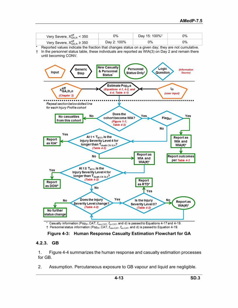
AMedP-7.5

4-13 SD.3

Very Severe, XGA,iheff < 350 0% Day 15: 100%† 0%

Very Severe, XGA,iheff ≥ 350 Day 2: 100% 0% 0%

* Reported values indicate the fraction that changes status on a given day; they are not cumulative. † In the personnel status table, these individuals are reported as WIA(3) on Day 2 and remain there

until becoming CONV.

Figure 4-3: Human Response Casualty Estimation Flowchart for GA

4.2.3. GB

1. Figure 4-4 summarizes the human response and casualty estimation processes for GB.

2. Assumption. Percutaneous exposure to GB vapour and liquid are negligible.

AMedP-7.5

4-14 SD.3

3. Inhalation is the only GB challenge type considered. Each icon’s inhaled Ct (XGB,ih,n

eff ) is estimated according to Chapter 3.

4. Special consideration for GB. If FlagMT = Yes, the user must further specify whether the available medical treatment includes only self-aid and buddy aid (individual issue autoinjectors), or if it also includes further medical treatment at a MTF. This choice is captured in the parameter MTGB, which can have the values “SABA” (self-aid/buddy aid) or “FMT” (further medical treatment). The default value is FMT. Using SABA may be warranted in MASCAL scenarios where it is anticipated that insufficient resources will be available.

5. For inhaled GB, Table 4-4 summarizes the toxicity parameters and associated symptoms, Table 4-5 fully describes the associated Injury Profiles, and Table 4-6 describes the outcomes associated with medical treatment.

Table 4-4: Inhaled GB Toxicity Parameters and Symptoms Injury

Profile Label ECt50

[mg-min/m3] Probit Slope

[probits/log(dose)]TLE Associated Symptoms

Mild 0.4 4.5 1.4 Miosis; rhinorrhea; transient chest tightness

Moderate 1.2 12 1.5

Rhinorrhea; blurred vision or eye pain with sensitivity to light; mild headache; excessive airway secretions induce frequent cough; nausea

Severe 25 12 1.5

Increased secretions and eye effects; vomiting; abdominal cramps; severe headache with anxiety and confusion; tight chest; twitching; weakness; diarrhea

Very Severe 33 12 1.5 Collapse and respiratory failure

Table 4-5: Inhaled GB Injury Profiles Time Point

(min) Injury Profile

Mild Moderate Severe Very Severe

1 0 2 3 4 3 1 2 3 4

15 1 2 3 4*

150 0 2 3 1000 0 2 2 1940 0 1 2 8640 0 1 1

* According to the default value for Tdeath-CN-SL4, death would be modeled at this point.

Table 4-6: GB Medical Treatment Outcome Reporting Injury Profile DOW* CONV* RTD*

Mild 0% Day 2: 100% Day 8: 100%

Moderate 0% Day 3: 100% Day 15: 100%

AMedP-7.5

4-15 SD.3

Injury Profile DOW* CONV* RTD*

Severe 0% Day 5: 33.3% Day 6: 33.3% Day 7: 33.4%

Day 31: 100%

If MTGB = SABA (self-aid/buddy aid only)

Very Severe, XGB,iheff < 100 0% Day 15: 100%† 0%

Very Severe, XGB,iheff ≥ 100 Day 2: 100% 0% 0%

If MTGB = FMT (self-aid/buddy aid + further medical treatment)

Very Severe, XGB,iheff < 165 0% Day 15: 100%† 0%

Very Severe, XGB,iheff ≥ 165 Day 2: 100% 0% 0%

* Reported values indicate the fraction that changes status on a given day; they are not cumulative. † In the personnel status table, these individuals are reported as WIA(3) on Day 2 and remain there

until becoming CONV.

Figure 4-4: Human Response Casualty Estimation Flowchart for GB

AMedP-7.5

4-16 SD.3

4.2.4. GD

1. Figure 4-5 summarizes the human response and casualty estimation processes for GD.

2. Assumption. Percutaneous exposure to GD vapour and liquid are negligible.

3. Inhalation is the only GD challenge type considered. Each icon’s inhaled Ct (XGD,ih,n

eff ) is estimated according to Chapter 3.

4. Special consideration for GD. If FlagMT = Yes, the user must further specify whether the available medical treatment includes only self-aid and buddy aid (individual issue autoinjectors), or if it also includes further medical treatment at a MTF. This choice is captured in the parameter MTGD, which can have the values “SABA” (self-aid/buddy aid) or “FMT” (further medical treatment). The default value is FMT. Using SABA may be warranted in MASCAL scenarios where it is anticipated that insufficient resources will be available. When FlagMT = Yes, it is assumed that all personnel have taken pyridostigmine bromide (PB) pretreatment.

5. For inhaled GD, Table 4-7 summarizes the toxicity parameters and associated symptoms, Table 4-8 fully describes the associated Injury Profiles, and Table 4-9 describes the outcomes associated with medical treatment.

Table 4-7: Inhaled GD Toxicity Parameters and Symptoms Injury

Profile Label ECt50

[mg-min/m3] Probit Slope

[probits/log(dose)]TLE Associated Symptoms

Mild 0.2 4.5 1.4 Miosis; rhinorrhea; transient chest tightness

Moderate 0.6 12 1.5

Rhinorrhea; blurred vision or eye pain with sensitivity to light; mild headache; excessive airway secretions induce frequent cough; nausea

Severe 25 12 1.5

Increased secretions and eye effects; vomiting; abdominal cramps; severe headache with anxiety and confusion; tight chest; twitching; weakness; diarrhea

Very Severe 33 12 1.5 Collapse and respiratory failure

AMedP-7.5

4-17 SD.3

Table 4-8: Inhaled GD Injury Profiles Time Point

(min) Injury Profile

Mild Moderate Severe Very Severe

1 0 2 3 4 3 1 2 3 4

15 1 2 3 4*

150 0 2 3 1000 0 2 2 1940 0 1 2 8640 0 1 1

* According to the default value for Tdeath-CN-SL4, death would be modeled at this point.

Table 4-9: GD Medical Treatment Outcome Reporting Injury Profile DOW* CONV* RTD*

Mild 0% Day 2: 100% Day 8: 100%

Moderate 0% Day 3: 100% Day 15: 100%

Severe 0% Day 5: 33.3% Day 6: 33.3% Day 7: 33.4%

Day 31: 100%

If MTGD = SABA (PB pretreatment + self-aid/buddy aid)

Very Severe, XGD,iheff < 100 0% Day 15: 100%† 0%

Very Severe, XGD,iheff ≥ 100 Day 2: 100% 0% 0%

If MTGD = FMT (PB pretreatment + self-aid/buddy aid + further medical treatment)

Very Severe, XGD,iheff < 165 0% Day 15: 100%† 0%

Very Severe, XGD,iheff ≥ 165 Day 2: 100% 0% 0%

* Reported values indicate the fraction that changes status on a given day; they are not cumulative. † In the personnel status table, these individuals are reported as WIA(3) on Day 2 and remain there

until becoming CONV.

AMedP-7.5

4-18 SD.3

Figure 4-5: Human Response Casualty Estimation Flowchart for GD

4.2.5. GF

1. Figure 4-6 summarizes the human response and casualty estimation processes for GF.

2. Assumption. Percutaneous exposure to GF vapour and liquid are negligible.

3. Inhalation is the only GF challenge type considered. Each icon’s inhaled Ct (XGF,ih,n

eff ) is estimated according to Chapter 3.

AMedP-7.5

4-19 SD.3

4. Special consideration for GF. If FlagMT = Yes, the user must further specify whether the available medical treatment includes only self-aid and buddy aid (individual issue autoinjectors), or if it also includes further medical treatment at a MTF. This choice is captured in the parameter MTGF, which can have the values “SABA” (self-aid/buddy aid) or “FMT” (further medical treatment). The default value is FMT. Using SABA may be warranted in MASCAL scenarios where it is anticipated that insufficient resources will be available.

5. For inhaled GF, Table 4-10 summarizes the toxicity parameters and associated symptoms, Table 4-11 fully describes the associated Injury Profiles, and Table 4-12 describes the outcomes associated with medical treatment.

Table 4-10: Inhaled GF Toxicity Parameters and Symptoms Injury

Profile Label ECt50

[mg-min/m3] Probit Slope

[probits/log(dose)]TLE Associated Symptoms

Mild 0.4 4.5 1.4 Miosis; rhinorrhea; transient chest tightness

Moderate 1.2 12 1.25

Rhinorrhea; blurred vision or eye pain with sensitivity to light; mild headache; excessive airway secretions induce frequent cough; nausea

Severe 31 12 1.25

Increased secretions and eye effects; vomiting; abdominal cramps; severe headache with anxiety and confusion; tight chest; twitching; weakness; diarrhea

Very Severe 41 12 1.25 Collapse and respiratory failure

Table 4-11: Inhaled GF Injury Profiles Time Point

(min) Injury Profile

Mild Moderate Severe Very Severe

1 0 2 3 4 3 1 2 3 4

15 1 2 3 4*

150 0 2 3 1000 0 2 2 1940 0 1 2 8640 0 1 1

* According to the default value for Tdeath-CN-SL4, death would be modeled at this point.

Table 4-12: GF Medical Treatment Outcome Reporting Injury Profile DOW* CONV* RTD*

Mild 0% Day 2: 100% Day 8: 100%

Moderate 0% Day 3: 100% Day 15: 100%

Severe 0% Day 5: 33.3% Day 6: 33.3% Day 7: 33.4%

Day 31: 100%

If MTGF = SABA (self-aid/buddy aid only)

Very Severe, XGF,iheff < 123 0% Day 15: 100%† 0%

AMedP-7.5

4-20 SD.3

Injury Profile DOW* CONV* RTD*

Very Severe, XGF,iheff ≥ 123 Day 2: 100% 0% 0%

If MTGF = FMT (self-aid/buddy aid + further medical treatment)

Very Severe, XGF,iheff < 205 0% Day 15: 100%† 0%

Very Severe, XGF,iheff ≥ 205 Day 2: 100% 0% 0%

* Reported values indicate the fraction that changes status on a given day; they are not cumulative. † In the personnel status table, these individuals are reported as WIA(3) on Day 2 and remain there

until becoming CONV.

Figure 4-6: Human Response Casualty Estimation Flowchart for GF

AMedP-7.5

4-21 SD.3

4.2.6. VX

1. Figure 4-7 summarizes the human response and casualty estimation processes for VX.

2. Assumption

a. Percutaneous exposure to VX vapour is negligible.

b. Human response due to inhaled VX and percutaneous VX liquid are independent of one another—the effects of each challenge type are modeled separately, and are only combined in the form of a Composite Injury Profile.

3. Inhalation and percutaneous liquid are the challenge types considered for VX. Each icon’s inhaled Ct (XVX,ih,n

eff ) and percutaneous liquid dose (XVX,pc,neff ) are estimated

according to Chapter 3.

4. Special consideration for VX. If FlagMT = Yes, the user must further specify whether the available medical treatment includes only self-aid and buddy aid (individual issue autoinjectors), or if it also includes further medical treatment at a MTF. This choice is captured in the parameter MTVX, which can have the values “SABA” (self-aid/buddy aid) or “FMT” (further medical treatment). The default value is FMT. Using SABA may be warranted in MASCAL scenarios where it is anticipated that insufficient resources will be available.

5. For inhaled VX, Table 4-13 summarizes the toxicity parameters and associated symptoms and Table 4-14 fully describes the associated Injury Profiles. Likewise, Table 4-15 and Table 4-16 describe the toxicity parameters, symptoms, Injury Profiles for percutaneous VX liquid. Finally, Table 4-17 describes the outcomes associated with medical treatment.

Table 4-13: Inhaled VX Toxicity Parameters and Symptoms Injury Profile

Label ECt50

[mg-min/m3] Probit Slope

[probits/log(dose)]TLE Associated Symptoms

Mild 0.04 4.5 1.4 Miosis; rhinorrhea; transient chest tightness

Moderate 0.12 12 1

Rhinorrhea; blurred vision or eye pain with sensitivity to light; mild headache; excessive airway secretions induce frequent cough; nausea

Severe 9 12 1

Increased secretions and eye effects; vomiting; abdominal cramps; severe headache with anxiety and confusion; tight chest; twitching; weakness; diarrhea

Very Severe 12 12 1 Collapse and respiratory failure

AMedP-7.5

4-22 SD.3

Table 4-14: Inhaled VX Injury Profiles Time Point

(min) Injury Profile

Mild Moderate Severe Very Severe

1 0 2 3 4 3 1 2 3 4

15 1 2 3 4*

150 0 2 3 1000 0 2 2 1940 0 1 2 8640 0 1 1

* According to the default value for Tdeath-CN-SL4, death would be modeled at this point.

Table 4-15: Percutaneous VX Liquid Toxicity Parameters and Symptoms Injury

Profile Label ECt50

[mg-min/m3] Probit Slope

[probits/log(dose)]TLE Associated Symptoms

Moderate 1.2 6 1 Muscle twitching; chest tightness and shortness of breath; episodes of vomiting

Severe 2 6 1

Severe generalized trembling with possible convulsions; feelings of confusion and anxiety; respiratory congestion and bronchorrhea

Very Severe 3 5.5 1 Unconsciousness; paralysis; breathing stops completely or struggling to breathe

Table 4-16: Percutaneous VX Liquid Injury Profiles Time Point

(min) Injury Profile Time Point

(min) Injury Profile

Moderate Severe Very Severe Moderate Severe Very Severe

1 0 0 0 100 1 2 8 0 1 1 150 1 3 10 1 1 1 360 2 3 30 1 1 2 1000 1 3 36 1 1 4 1440 0 3 51 1 1 4* 2400 0 2

* According to the default value for Tdeath-CN-SL4, death would be modeled at this point.

6. Medical treatment-related outcomes for icons challenged via both inhalation and percutaneous liquid are dictated by the more severe challenge, where the severity of the challenge increases as one moves down the rows in Table 4-17.

AMedP-7.5

4-23 SD.3

Table 4-17: VX Medical Treatment Outcome Reporting

Inhalation Injury Profile Percutaneous Injury

Profile DOW* CONV* RTD*

Mild (n/a) 0% Day 2: 100% Day 8: 100%

Moderate Moderate 0% Day 3: 100% Day 15: 100%

Severe Severe 0% Day 5: 33.3% Day 6: 33.3% Day 7: 33.4%

Day 31: 100%

If MTVX = SABA (self-aid/buddy aid only)

Very Severe, XVX,iheff < 36 Very Severe, XVX,pc,n

eff < 9 0% Day 15: 100%† 0%

Very Severe, XVX,iheff ≥ 36 Very Severe, XVX,pc,n

eff < 9 Day 2: 100% 0% 0%

If MTVX = FMT (self-aid/buddy aid + further medical treatment)

Very Severe, XVX,iheff < 60 Very Severe, XVX,pc,n

eff < 15 0% Day 15: 100%† 0%

Very Severe, XVX,iheff ≥ 60 Very Severe, XVX,pc,n

eff < 15 Day 2: 100% 0% 0%

* Reported values indicate the fraction that changes status on a given day; they are not cumulative. † In the personnel status table, these individuals are reported as WIA(3) on Day 2 and remain there

until becoming CONV.

AMedP-7.5

4-24 SD.3

Figure 4-7: Human Response and Casualty Estimation Flowchart for VX

AMedP-7.5

4-25 SD.3

4.2.7. HD

1. Figure 4-8 summarizes the human response and casualty estimation processes for HD.

2. Assumption. Human response due to inhaled HD, percutaneous HD vapour, and percutaneous HD liquid are independent of one another—the effects of each challenge type are modeled separately, and are only combined in the form of Composite Injury Profiles and the Equivalent Percutaneous Vapour challenge type.

3. Inhalation, ocular vapour, and equivalent percutaneous vapour (which contains contributions from percutaneous liquid and percutaneous vapour—see Table 2-2) are the challenge types considered for HD.

a. Each icon’s inhaled Ct (XHD,ih,neff ) is estimated according to Chapter 3.

b. Each icon’s ocular vapour Ct (XHD,oc,neff ) is estimated according to Chapter 3,

using percutaneous vapour data as input; the ocular vapour Ct is considered equivalent to the percutaneous vapour Ct.

c. Each icon’s equivalent percutaneous vapour Ct (XHD,epc,k,neff ) is estimated using

both percutaneous vapour and percutaneous liquid input data, according to Equation 4-21.60 Because Equation 4-21 contains a term whose value depends upon the health effect being considered (lethal or mild/severe), the symbol for equivalent percutaneous vapour Ct contains k in its subscript. Further, XHD,epc,lethal,n

eff and XHD,epc,mild/severe,neff must both be computed, and each

must be used appropriately when calculating the populations of Injury Profile cohorts in accordance with Section 4.1.2.

XHD,epc,k,neff = XHD,pv,n

eff + XHD,pl,neff · CFHD,k, (4-21)

where:

XHD,epc,k,neff is the equivalent percutaneous vapour Ct for icon n [mg-min/m3],

XHD,pv,neff is the percutaneous vapour Ct for icon n as calculated according

to Chapter 3 [mg-min/m3],

XHD,pl,neff is the percutaneous liquid dose for icon n as calculated according

to Chapter 3 [mg], and

CFHD,k is the percutaneous liquid to equivalent vapour conversion factor for HD [(mg-min/m3) / (mg)], as defined in Equation 4-22.

60 Gene E. McClellan, George H. Anno, and Leigh N. Matheson, Consequence Analytic Tools for NBC Operations Volume 3: Chemical Agent Exposure and Casualty Estimation (Alexandria, VA: Defense Special Weapons Agency, 1998), 32–35.

AMedP-7.5

4-26 SD.3

CFHD,k= vapour toxicity

liquid toxicity, (4-22)

where:

k can be “lethal” or “mild/severe”,

vapour toxicity is either the ECt50-severe (when k is “mild/severe”) or the LCt50 (when k is “lethal”) listed in Table 4-18, and

liquid toxicity is either the ED50-severe (when k is “mild/severe”)or the LD50 (when k is “lethal”) listed in Table 4-18.

Table 4-18: Recommended Parameter Values for Equivalent Vapour Conversion Factors for HD (CFHD,k)

Toxicity Parameter Recommended Parameter Value*

ECt50-severe (percutaneous vapour) 500 mg-min/m3

ED50-severe (percutaneous liquid) 600 mg

LCt50 (percutaneous vapour) 10,000 mg-min/m3

LD50 (percutaneous liquid) 1,400 mg * U.S. Army Chemical School (USACMLS), Potential Military Chemical/Biological Agents and

Compounds, FM 3-11.9/MCRP 3-37.1B/NTRP 3–11.32/AFTTP(I) 3-2.55 (Washington, DC: U.S. Government Printing Office, January 2005), II-40.

4. For inhaled HD, Table 4-19 summarizes the toxicity parameters and associated symptoms and Table 4-20 fully describes the associated Injury Profiles. Likewise, Table 4-21 and Table 4-22 describe the symptoms and Injury Profiles for ocular HD vapour, and Table 4-23 and Table 4-24 describe the symptoms and Injury Profiles for equivalent percutaneous HD vapour. Finally, Table 4-25 describes the outcomes associated with medical treatment.

Table 4-19: Inhaled HD Toxicity Parameters and Symptoms Injury Profile

Label ECt50

[mg-min/m3] Probit Slope

[probits/log(dose)]TLE Associated Symptoms

IH Mild, XHD,ih

eff < 70 72 6 1.5

Nauseated; swallows often

IH Mild, XHD,ih

eff ≥ 70

Dry mouth; dry cough; sneezing; runny nose; headache; nauseated; vomited once or twice

IH Moderate 145 6 1.5 Sore throat; continuous cough; hoarseness; chest feels tight; headache; fever

IH Severe 220 6 1.5 Hurts to breathe; hacking cough; cannot speak; headache; dry heaves; fatigued from vomiting

IH Very Severe, XHD,ih

eff < 1200 1000 6 1.5

Awful chest pain; wheezing and shortness of breath; coughs up red colored mucous IH Very Severe,

XHD,iheff ≥ 1200

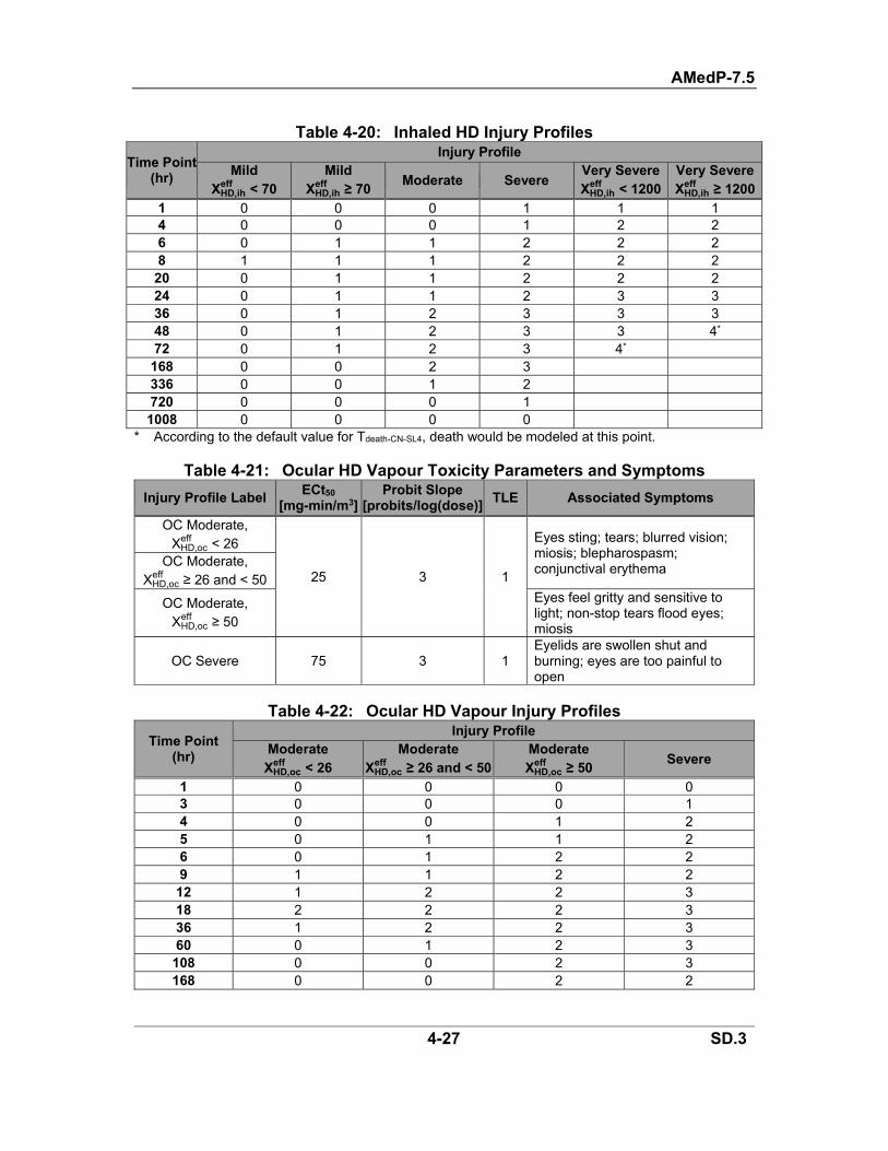
AMedP-7.5

4-27 SD.3

Table 4-20: Inhaled HD Injury Profiles

Time Point (hr)

Injury Profile Mild

XHD,iheff < 70

Mild XHD,ih

eff ≥ 70 Moderate Severe Very Severe XHD,ih

eff < 1200

Very Severe XHD,ih

eff ≥ 1200

1 0 0 0 1 1 14 0 0 0 1 2 2 6 0 1 1 2 2 2 8 1 1 1 2 2 2

20 0 1 1 2 2 2 24 0 1 1 2 3 3 36 0 1 2 3 3 3 48 0 1 2 3 3 4*

72 0 1 2 3 4* 168 0 0 2 3 336 0 0 1 2 720 0 0 0 1 1008 0 0 0 0

* According to the default value for Tdeath-CN-SL4, death would be modeled at this point.

Table 4-21: Ocular HD Vapour Toxicity Parameters and Symptoms

Injury Profile Label ECt50

[mg-min/m3]Probit Slope

[probits/log(dose)]TLE Associated Symptoms

OC Moderate, XHD,oc

eff < 26

25 3 1

Eyes sting; tears; blurred vision; miosis; blepharospasm; conjunctival erythema OC Moderate,

XHD,oceff ≥ 26 and < 50

OC Moderate, XHD,oc

eff ≥ 50

Eyes feel gritty and sensitive to light; non-stop tears flood eyes; miosis

OC Severe 75 3 1 Eyelids are swollen shut and burning; eyes are too painful to open

Table 4-22: Ocular HD Vapour Injury Profiles

Time Point (hr)

Injury Profile Moderate XHD,oc

eff < 26

ModerateXHD,oc

eff ≥ 26 and < 50ModerateXHD,oc

eff ≥ 50 Severe

1 0 0 0 0 3 0 0 0 1 4 0 0 1 2 5 0 1 1 2 6 0 1 2 2 9 1 1 2 2

12 1 2 2 3 18 2 2 2 3 36 1 2 2 3 60 0 1 2 3

108 0 0 2 3 168 0 0 2 2

AMedP-7.5

4-28 SD.3

Time Point (hr)

Injury Profile Moderate XHD,oc

eff < 26

ModerateXHD,oc

eff ≥ 26 and < 50ModerateXHD,oc

eff ≥ 50 Severe

504 0 0 1 1 672 0 0 0 0

Table 4-23: Equivalent Percutaneous HD Vapour Toxicity Parameters and Symptoms

Injury Profile Label

ECt50 [mg-min/m3]

Probit Slope [probits/log(dose)]

TLE Associated Symptoms

EPC Mild, XHD,epc

eff < 125 25 3 1

Skin sensitive to touch in tender areas (crotch, armpits, inside of elbow and knee)

EPC Mild, XHD,epc

eff ≥ 125

Skin sore in tender areas; painful when moving; redness of the skin; tiny blisters on hands and neck

EPC Severe 380 3 1 Skin peels off leaving open raw areas and painful ulcers in tender areas

EPC Very Severe 10,000 7 1

Skin symptoms from above, plus eventual death due to secondary effects related to bone marrow stem cell depression

Table 4-24: Equivalent Percutaneous HD Vapour Injury Profiles

Time Point (hr)

Injury Profile Mild

XHD,epceff < 125

MildXHD,epc

eff ≥ 125 Severe Very Severe

1 0 0 0 0 2 0 0 1 1 5 0 0 2 2

18 0 1 2 2 24 0 1 3 3 36 1 1 3 3 96 0 1 3 3

168 0 0 3 3 336 0 0 3 4*

504 0 0 1 588 0 0 0

* Death is modeled at this point regardless of the values of the various methodology parameters.

AMedP-7.5

4-29 SD.3

Table 4-25: HD Medical Treatment Outcome Reporting Injury Profile DOW* CONV* RTD*

Inhalation Injury Profiles

IH Mild, XHD,iheff < 70 0% 0%

Day 2: 50% Day 3: 50%

IH Mild, XHD,iheff ≥ 70 0% 0%

Day 2: 14% Day 3: 15% Day 4: 14% Day 5: 14% Day 6: 14% Day 7: 14% Day 8: 15%

IH Moderate 0%

Day 21: 5% Day 28: 24% Day 35: 4% Day 42: 10% Day 49: 57%

0%

IH Severe 0%

Day 35: 25% Day 42: 25% Day 49: 25% Day 56: 25%

0%

IH Very Severe, XHD,iheff < 1200

Day 7: 17% Day 14: 83%

0% 0%

IH Very Severe, XHD,iheff ≥ 1200 Day 3: 100% 0% 0%

Ocular Injury Profiles

OC Moderate XHD,oceff < 26 0% 0%

Day 2: 50% Day 3: 100%

OC Moderate, XHD,oceff ≥ 26 and < 50 0% Day 14: 100% 0%

OC Moderate XHD,oceff ≥ 50 0%

Day 21: 33% Day 28: 33% Day 35: 34%

0%

OC Severe 0%

Day 63: 25% Day 70: 25% Day 77: 25% Day 84: 25%

0%

Equivalent Percutaneous Injury Profiles

EPC Mild XHD,epceff < 125 0% 0%

Day 2: 33% Day 3: 33% Day 4: 34%

EPC Mild XHD,epceff ≥ 125 0% Day 4: 100% 0%

EPC Severe 0%

Day 28: 26% Day 35: 7% Day 49: 34% Day 56: 20% Day 70: 13%

0%

EPC Very Severe Day 7: 100% 0% 0% * Reported values indicate the fraction that changes status on a given day; they are not cumulative.

AMedP-7.5

4-30 SD.3

Figure 4-8: Human Response and Casualty Estimation Flowchart for HD

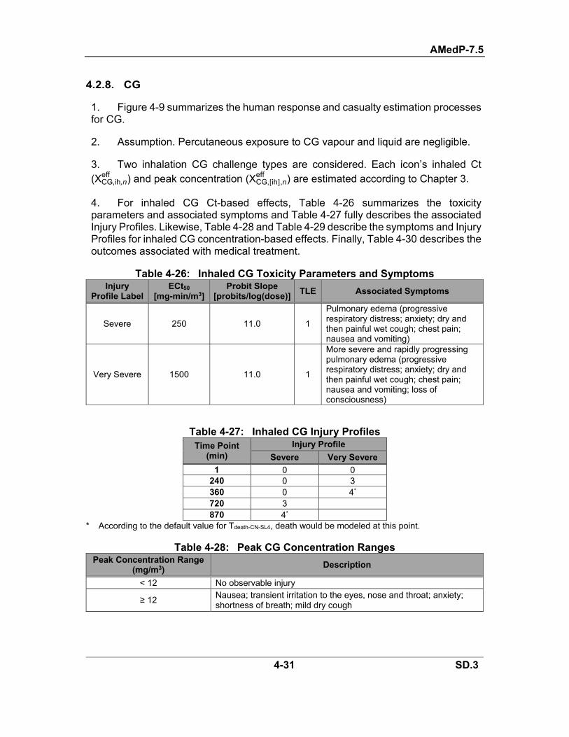
AMedP-7.5

4-31 SD.3

4.2.8. CG

1. Figure 4-9 summarizes the human response and casualty estimation processes for CG.

2. Assumption. Percutaneous exposure to CG vapour and liquid are negligible.

3. Two inhalation CG challenge types are considered. Each icon’s inhaled Ct (XCG,ih,n

eff ) and peak concentration (XCG, ih ,neff ) are estimated according to Chapter 3.

4. For inhaled CG Ct-based effects, Table 4-26 summarizes the toxicity parameters and associated symptoms and Table 4-27 fully describes the associated Injury Profiles. Likewise, Table 4-28 and Table 4-29 describe the symptoms and Injury Profiles for inhaled CG concentration-based effects. Finally, Table 4-30 describes the outcomes associated with medical treatment.

Table 4-26: Inhaled CG Toxicity Parameters and Symptoms Injury

Profile Label ECt50

[mg-min/m3] Probit Slope

[probits/log(dose)]TLE Associated Symptoms

Severe 250 11.0 1

Pulmonary edema (progressive respiratory distress; anxiety; dry and then painful wet cough; chest pain; nausea and vomiting)

Very Severe 1500 11.0 1

More severe and rapidly progressing pulmonary edema (progressive respiratory distress; anxiety; dry and then painful wet cough; chest pain; nausea and vomiting; loss of consciousness)

Table 4-27: Inhaled CG Injury Profiles Time Point

(min) Injury Profile

Severe Very Severe

1 0 0 240 0 3 360 0 4*

720 3 870 4*

* According to the default value for Tdeath-CN-SL4, death would be modeled at this point.

Table 4-28: Peak CG Concentration Ranges Peak Concentration Range

(mg/m3) Description

< 12 No observable injury

≥ 12 Nausea; transient irritation to the eyes, nose and throat; anxiety; shortness of breath; mild dry cough

AMedP-7.5

4-32 SD.3

Table 4-29: Peak CG Concentration Injury Profile Time Point

(min) Injury Profile

≥ 12 mg/m3

1 115 0

Table 4-30: CG Medical Treatment Outcome Reporting Injury Profile DOW* CONV* RTD*

> 12 mg/m3 0% 0% Day 2: 100%

Severe 0%

Day 14: 2%† Day 21: 7%† Day 28: 12%† Day 35: 17%† Day 42: 22%† Day 49: 25%† Day 56: 13%† Day 60: 2%†

Day 90: 100%

Very Severe Day 2: 100% 0% 0% * Reported values indicate the fraction that changes status on a given day; they are not cumulative. † In the personnel status table, these individuals are reported as WIA(3) on Day 2 and remain there

until becoming CONV.

AMedP-7.5

4-33 SD.3

Figure 4-9: Human Response and Casualty Estimation Flowchart for CG

AMedP-7.5

4-34 SD.3

4.2.9. Cl2

1. Figure 4-10 summarizes the human response and casualty estimation processes for Cl2.

2. Assumption. Percutaneous exposure to Cl2 vapour and liquid are negligible.

3. Inhalation is the only Cl2 challenge type considered. Each icon’s inhaled Ct (XCl2,ih,n

eff ) is estimated according to Chapter 3.

4. For inhaled Cl2, Table 4-31 summarizes the toxicity parameters and associated symptoms, Table 4-32 fully describes the associated Injury Profiles, and Table 4-33 describes the outcomes associated with medical treatment.

Table 4-31: Inhaled Cl2 Toxicity Parameters and Symptoms Injury

Profile Label ECt50

[mg-min/m3] Probit Slope

[probits/log(dose)]TLE Associated Symptoms

Mild 70 10.5 2.75

Nausea; desire to vomit; mild eye irritation; mild shortness of breath; chest tightness, slight irritation of nose and throat; cough; minor nasal congestion and runny nose; headache and dizziness

Moderate 325 10.5 2.75

Vomiting; severe eye irritation; moderate shortness of breath; some chest pain; difficulty breathing; more pronounced coughing and irritation of the throat; nasal and respiratory congestion with possible phlegm

Severe 1300 10.5 2.75

Severe shortness of breath; marked chest pain; rapid and restricted breathing; intense coughing; tracheo-bronchitis; delayed onset of pulmonary edema and/or toxic pneumonitis or bronchio-pneumonia

Very Severe 13500 10.5 2.75

Extreme shortness of breath; decreased breath sounds; production of large amounts of frothy liquid; rapid onset of pulmonary edema; coma; death

Table 4-32: Inhaled Cl2 Injury Profiles Time Point

(min) Injury Profile

Mild Moderate Severe Very Severe

1 1 2 2 3 120 1 2 3 4 135 1 2 3 4* 360 0 2 3 720 0 1 3 1440 0 0 3

10080 0 0 0 * According to the default value for Tdeath-CN-SL4, death would be modeled at this point.

AMedP-7.5

4-35 SD.3

Table 4-33: Cl2 Medical Treatment Outcome Reporting Injury Profile DOW* CONV* RTD*

Mild 0% 0% Day 2: 100%

Moderate 0% 0% Day 2: 100%

Severe 0% 0% Day 5: 100%

Very Severe Day 2: 7%

Day 7: 27%† Day 14: 22%† Day 21: 22%† Day 28: 22%†

Day 60: 93%

* Reported values indicate the fraction that changes status on a given day; they are not cumulative. † In the personnel status table, these individuals are reported as WIA(3) on Day 2 and remain there

until becoming CONV.

Figure 4-10: Human Response and Casualty Estimation Flowchart for Cl2

AMedP-7.5

4-36 SD.3

4.2.10. NH3

1. Figure 4-11 summarizes the human response and casualty estimation processes for NH3.

2. Assumption. Percutaneous exposure to NH3 vapour and liquid are negligible.

3. Inhalation is the only NH3 challenge type considered. Each icon’s inhaled Ct (XNH3,ih,n

eff ) is estimated according to Chapter 3.

4. For inhaled NH3, Table 4-34 summarizes the toxicity parameters and associated symptoms, Table 4-35 fully describes the associated Injury Profiles, and Table 4-36 describes the outcomes associated with medical treatment.

Table 4-34: Inhaled NH3 Toxicity Parameters and Symptoms Injury

Profile Label ECt50

[mg-min/m3] Probit Slope

[probits/log(dose)]TLE Associated Symptoms

Mild 350 16.5 2.0 Mild eye irritation; rhinorrhea; cough; sneezing; drooling; dyspnea; headache

Moderate 1000 16.5 2.0

Tear production; burning sensation; blepharospasm; conjunctivitis; photophobia; more pronounced cough; pharyngitis; laryngitis; moderate throat irritation

Severe 7800 16.5 2.0

Corneal ulcerations; iritis; anterior and posterior synechia; corneal opacification; cataracts; glaucoma; retinal atrophy; directly caustic to airway; laryngospasm; bronchospasm; chest pain; loss of consciousness

Very Severe 67700 16.5 2.0

Sloughing and necrosis of airway mucosa; severe chest pain; pulmonary edema; respiratory failure; cerebral edema; seizures; coma; death

Table 4-35: Inhaled NH3 Injury Profiles Time Point

(min) Injury Profile

Mild Moderate Severe Very Severe

1 1 2 2 4 15 1 2 2 4*

360 0 2 2

720 0 2 3 4320 0 0 3

43200 0 0 0 * According to the default value for Tdeath-CN-SL4, death would be modeled at this point.

AMedP-7.5

4-37 SD.3

Table 4-36: NH3 Medical Treatment Outcome Reporting Injury Profile DOW* CONV* RTD*

Mild 0 0 Day 2: 100%

Moderate 0 0 Day 4: 100%

Severe 0 0 Day 8: 100%

Very Severe Day 31: 27% Day 15: 36%† Day 29: 37%†

Day 91: 73%

* Reported values indicate the fraction that changes status on a given day; they are not cumulative. † In the personnel status table, these individuals are reported as WIA(3) on Day 2 and remain there

until becoming RTD.

Figure 4-11: Human Response and Casualty Estimation Flowchart for NH3

AMedP-7.5

4-38 SD.3

4.2.11. AC

1. Figure 4-12 summarizes the human response and casualty estimation processes for AC.

2. Assumption. Percutaneous exposure to AC vapour and liquid are negligible.

3. Inhalation is the only AC challenge type considered. Each icon’s inhaled Ct (XAC,ih,n

eff ) is estimated according to Chapter 3.

4. Special consideration for AC. Even when FlagMT = Yes, medical treatment will not have any effect unless the user sets TMTF ≤ Tdeath-CN-SL4. If this is done, the user may then also choose between whether that treatment involves supportive care alone, or supportive care plus antidote treatment. This choice is captured in the parameter MTAC, which can have the values “SC” (supportive care) or “AT” (antidote treatment). The default value is AT. Using SC may be warranted in MASCAL scenarios where it is anticipated that insufficient resources will be available.

5. For inhaled AC, Table 4-37 summarizes the toxicity parameters and associated symptoms, Table 4-38 fully describes the associated Injury Profiles, and Table 4-39 describes the outcomes associated with medical treatment.

Table 4-37: Inhaled AC Toxicity Parameters and Symptoms Injury

Profile Label ECt50

[mg-min/m3] Probit Slope

[probits/log(dose)]TLE Associated Symptoms

Mild 700 12.0 2.0

Nausea; fatigue and weakness; transient rapid breathing followed by slower breathing; shortness of breath; excitement; anxiety; dizziness; headache

Moderate 1100 12.0 2.0

Episodes of vomiting; increased fatigue and weakness; muscle spasms; difficult to breathe; drowsiness

Severe 1400 12.0 2.0

Severe generalized twitching with or without convulsions; breathing sporadically stops and starts; unconsciousness

Very Severe 2600 12.0 2.0 Convulsions; breathing stops completely; coma

AMedP-7.5

4-39 SD.3

Table 4-38: Inhaled AC Injury Profiles Time Point

(min) Injury Profile

Mild Moderate Severe Very Severe

1 1 2 3 4 10 1 1 2 4 15 1 1 2 4*

120 0 1 1 180 0 0 1 480 0 0 0

* According to the default value for Tdeath-CN-SL4, death would be modeled at this point.

Table 4-39: AC Medical Treatment Outcome Reporting Injury Profile DOW* CONV* RTD*

Mild 0% 0% Day 2: 100%

Moderate 0% 0% Day 2: 100%

Severe 0% 0% Day 2: 100%

If TMTF ≤ Tdeath-CN-SL4 and MTAC = SC

Very Severe, XAC,iheff < 5,200 0% 0% Day 6: 100%†

Very Severe, XAC,iheff ≥ 5,200 Day 2: 100% 0% 0%

If TMTF ≤ Tdeath-CN-SL4 and MTAC = AT

Very Severe, XAC,iheff < 26,000 0% 0% Day 4: 100%†

Very Severe, XAC,iheff ≥ 26,000 Day 2: 100% 0% 0%

Note: If TMTF > Tdeath-CN-SL4 (as is the default—see Table 2-14), the Very Severe cohort is KIA, so this table is not needed to estimate their outcome.

* Reported values indicate the fraction that changes status on a given day; they are not cumulative. † In the personnel status table, these individuals are reported as WIA(3) on Day 2 and remain there

until becoming RTD.

AMedP-7.5

4-40 SD.3

Figure 4-12: Human Response and Casualty Estimation Flowchart for AC

AMedP-7.5

4-41 SD.3

4.2.12. CK

1. Figure 4-13 summarizes the human response and casualty estimation processes for CK.

2. Assumption. Percutaneous exposure to CK vapour and liquid are negligible.

3. Inhalation is the only CK challenge type considered. Each icon’s inhaled Ct (XCK,ih,n

eff ) and peak concentration (XCK, ih ,neff ) are estimated according to Chapter 3.

4. Special consideration for CK. Even when FlagMT = Yes, medical treatment will not have any effect unless the user sets TMTF ≤ Tdeath-CN-SL4. If this is done, the user may then also choose between whether that treatment involves supportive care alone, or supportive care plus antidote treatment. This choice is captured in the parameter MTCK, which can have the values “SC” (supportive care) or “AT” (antidote treatment). The default value is AT. Using SC may be warranted in MASCAL scenarios where it is anticipated that insufficient resources will be available.

5. For inhaled CK Ct-based effects, Table 4-40 summarizes the toxicity parameters and associated symptoms and Table 4-41 fully describes the associated Injury Profiles. Likewise, Table 4-42 and Table 4-43 describe the symptoms and Injury Profiles for inhaled CK concentration-based effects. Finally, Table 4-44 describes the outcomes associated with medical treatment.

Table 4-40: Inhaled CK Toxicity Parameters and Symptoms Injury

Profile Label ECt50

[mg-min/m3] Probit Slope

[probits/log(dose)]TLE Associated Symptoms

Mild 1200 12.0 1.45

Nausea; fatigue and weakness; transient rapid breathing followed by slower breathing; shortness of breath; excitement; anxiety; dizziness; headache

Moderate 2100 12.0 1.45

Episodes of vomiting; increased fatigue and weakness; muscle spasms; difficult to breathe; drowsiness

Severe 2800 12.0 1.45

Severe generalized twitching with or without convulsions; breathing sporadically stops and starts; unconsciousness

Very Severe 4700 12.0 1.45 Convulsions; breathing stops completely; coma

AMedP-7.5

4-42 SD.3

Table 4-41: Inhaled CK Injury Profiles Time Point

(min) Injury Profile

Mild Moderate Severe Very Severe

1 1 2 3 4 10 1 1 2 4 15 1 1 2 4*

120 0 1 1 180 0 0 1 480 0 0 0

* According to the default value for Tdeath-CN-SL4, death would be modeled at this point.

Table 4-42: Peak CK Concentration Ranges Peak Concentration Range

(mg/m3) Description

< 1 No observable injury

1 – < 20 Ocular and upper respiratory irritation ≥ 20 Severe, but not intolerable, ocular and upper respiratory irritation

Table 4-43: Peak CK Concentration Injury Profiles Time Point

(min) Peak Concentration Range

1 – < 20 mg/m3 ≥ 20 mg/m3

1 1 2 2 0 1 10 0 0

Table 4-44: CK Medical Treatment Outcome Reporting Injury Profile DOW* CONV* RTD*

1 – < 20 mg/m3 0% 0% Day 2: 100%

≥ 20 mg/m3 0% 0% Day 2: 100%

Mild 0% 0% Day 2: 100%

Moderate 0% 0% Day 2: 100%

Severe 0% 0% Day 2: 100%

If TMTF ≤ Tdeath-CN-SL4 and MTCK = SC

Very Severe, XCK,iheff < 9,400 0% 0% Day 6: 100%†

Very Severe, XCK,iheff ≥ 9,400 Day 2: 100% 0% 0%

If TMTF ≤ Tdeath-CN-SL4 and MTCK = AT

Very Severe, XCK,iheff < 47,000 0% 0% Day 4: 100%†

Very Severe, XCK,iheff ≥ 47,000 Day 2: 100% 0% 0%

Note: If TMTF > Tdeath-CN-SL4 (as is the default—see Table 2-14), the Very Severe cohort is KIA, so this table is not needed to estimate their outcome.

* Reported values indicate the fraction that changes status on a given day; they are not cumulative. † In the personnel status table, these individuals are reported as WIA(3) on Day 2 and remain there

until becoming RTD.

AMedP-7.5

4-43 SD.3

Figure 4-13: Human Response and Casualty Estimation Flowchart for CK

4.2.13. H2S

1. Figure 4-14 summarizes the human response and casualty estimation

AMedP-7.5

4-44 SD.3

processes for H2S.

2. Assumption. Percutaneous exposure to H2S vapour and liquid are negligible.

3. Inhalation is the only H2S challenge type considered. Each icon’s inhaled Ct (XH2S,ih,n

eff ) is estimated according to Chapter 3.

4. For inhaled H2S, Table 4-45 summarizes the toxicity parameters and associated symptoms, Table 4-46 fully describes the associated Injury Profiles, and Table 4-47 describes the outcomes associated with medical treatment.

Table 4-45: Inhaled H2S Toxicity Parameters and Symptoms Injury

Profile Label ECt50

[mg-min/m3] Probit Slope

[probits/log(dose)]TLE Associated Symptoms

Mild 400 18.0 5.7

Nausea; fatigue and weakness; transient rapid breathing followed by slower breathing; shortness of breath; excitement; anxiety; dizziness; headache; gritty feeling in eyes; lacrimation; respiratory irritation; olfactory paralysis; cough

Moderate 1500 18.0 5.7

Episodes of vomiting; increased fatigue and weakness; muscle spasms; difficult to breathe; drowsiness; severe eye irritation; blurry vision; sensitivity to light; stronger respiratory irritation

Severe 2200 18.0 5.7

Severe generalized twitching with or without convulsions; breathing sporadically stops and starts; unconsciousness

Very Severe 3200 18.0 5.7 Convulsions; breathing stops completely; coma

Table 4-46: Inhaled H2S Injury Profiles Time Point

(min) Injury Profile

Mild Moderate Severe Very Severe

1 1 2 3 4 10 1 1 2 4 15 1 1 2 4*

60 0 1 2 120 0 0 2 300 0 0 1 2880 0 0 0

* According to the default value for Tdeath-CN-SL4, death would be modeled at this point.

Table 4-47: H2S Medical Treatment Outcome Reporting Injury Profile DOW* CONV* RTD*

Mild 0% 0% Day 2: 100%

Moderate 0% 0% Day 2: 100%

AMedP-7.5

4-45 SD.3

Injury Profile DOW* CONV* RTD*

Severe 0% 0% Day 3: 100%

If TMTF ≤ Tdeath-CN-SL4

Very Severe, XH2S,iheff < 6,400 0% 0% Day 21: 100%†

Very Severe, XH2S,iheff ≥ 6,400 Day 21: 100% 0% 0%

Note: If TMTF > Tdeath-CN-SL4 (as is the default—see Table 2-14), the Very Severe cohort is KIA, so this table is not needed to estimate their outcome.

* Reported values indicate the fraction that changes status on a given day; they are not cumulative. † In the personnel status table, these individuals are reported as WIA(3) on Day 2 and remain there

until becoming RTD.

Figure 4-14: Human Response and Casualty Estimation Flowchart for H2S

AMedP-7.5

4-46 SD.3

4.3. RADIOLOGICAL AGENT MODELS

This section begins with a discussion of assumptions and limitations that apply only to radiological agents. Next are separate sections for RDDs and fallout that describe special methods for estimating Effective CBRN Challenge and provide a flowchart summarizing the process from Effective CBRN Challenge to casualty estimate. Following the RDD and fallout sections are two additional sections used for both RDDs and fallout:

a. Dose ranges, Injury Profiles, and medical treatment outcome reporting tables.

b. Special considerations for casualty estimation.

4.3.1. Assumptions and Limitation

1. Assumptions

a. Individuals will decontaminate the skin after exiting the radiation area.

b. Human response is independent of the source of exposure. For example, whole-body radiation Injury Profiles for radiological incidents are identical to those used for whole-body radiation under the nuclear effects models.

c. Human response due to whole-body radiation dose and cutaneous radiation dose are independent of one another—the effects of each challenge type are modeled separately, and are only combined via a Composite Injury Profile.

d. For the purpose of estimating time to death due to whole-body radiation, each icon’s dose rate is equal to the icon’s total whole-body dose divided by the time during which the dose accumulated.

2. Limitation. Dose protraction—a sufficiently low dose rate such that some physiological recovery occurs simultaneously with the challenge—is only included as it pertains to determining whether a casualty will die; the Injury Profiles do not account for dose protraction.

4.3.2. RDDs

1. Figure 4-15 summarizes the human response and casualty estimation processes for RDDs.

2. Assumptions, limitations, and constraint.

a. Assumptions.

1) The activity deposited on the ground at the icon’s location is equal to the activity deposited on the skin of each individual in the icon.

2) For calculations of dose due to groundshine, the activity concentration at

AMedP-7.5

4-47 SD.3

the icon’s location for the time period of interest is uniformly extended to infinity in all directions.

3) For the purpose of deriving the dose conversion factors in Table 3-1, absorbed dose (in units of gray) is equal to dose equivalent (in units of Sievert).

4) Cutaneous dose due to beta emitters contaminating the clothing is negligible61 (contamination of the skin is counted).

5) The dose from inhalation of radiological particles is equal to the 30-day committed effective dose equivalent, and can be combined with the cloudshine and groundshine doses to determine an overall whole-body dose.

b. Limitations.

1) Conventional casualties (i.e., from high explosives and fragmentation) that might occur as part of a RDD incident are ignored.

2) Gamma radiation due to skin contamination is ignored because it is typically only a few percent of the beta radiation dose.62

c. Constraint. Because the user is forced to choose either a gamma radiation protection factor or a beta radiation protection factor for each isotope, that protection factor is applied to all radiation emitted by that isotope.

3. Whole-body radiation (from cloudshine, groundshine, and inhalation) and cutaneous radiation (from cloudshine, groundshine, and skin contamination) are the challenge types considered for RDDs.

a. Whole-body radiation.

1) Note that the cloudshine and groundshine components of whole-body radiation from RDDs can be a mix of different types of radiation. In calculating the APF, appropriate protection factors (from Table 2-7) must be chosen for each isotope, based on the type of radiation it primarily emits—see the footnote on Table 3-1.

2) Each icon’s isotope-specific absorbed whole-body dose from cloudshine from an RDD (XRDD,wb,cld,r,n

eff ) is estimated according to Chapter 3. Then, the

61 T. J. Cerveney, T. J. MacVittie, and R. W. Young, “Acute Radiation Syndrome in Humans,” in Warfare, Weaponry, and the Casualty, ed. Richard I. Walker and T. J. Cerveney, Textbooks of Military Medicine (Falls Church, VA: Office of the Surgeon General, Department of the Army, 1996), 15–36, 21. 62 IAEA, Generic Procedures for a Radiological Emergency, 104.

AMedP-7.5

4-48 SD.3

isotope-specific doses are summed to determine the total absorbed whole-body dose from cloudshine from an RDD (XRDD,wb,cld,n

eff ), according to Equation 4-23.

XRDD,wb,cld,neff = XRDD,wb,cld,r,n

eff

r

, (4-23)

where:

XRDD,wb,cld,neff is the absorbed whole-body cloudshine dose from an RDD

for icon n [Gy], and

XRDD,wb,cld,r,neff is the absorbed whole-body cloudshine dose from the rth

radioisotope from an RDD for icon n [Gy] (derived according to Chapter 3, from the output of the user’s national hazard prediction model).

3) Each icon’s isotope-specific absorbed whole-body dose from groundshine from an RDD (XRDD,wb,grd,r,n

eff ) is estimated according to Chapter 3. Then, the isotope-specific doses are summed to determine the total absorbed whole-body dose from groundshine from an RDD (XRDD,wb,grd,n

eff ), according to Equation 4-24.

XRDD,wb,grd,neff = XRDD,wb,grd,r,n

eff

r

, (4-24)

where:

XRDD,wb,grd,neff is the absorbed whole-body groundshine dose from an

RDD for icon n [Gy], and

XRDD,wb,grd,r,neff is the absorbed whole-body groundshine dose from the rth

radioisotope from an RDD for icon n [Gy] (derived according to Chapter 3, from the output of the user’s national hazard prediction model).

4) Each icon’s isotope-specific absorbed whole-body dose from inhalation of radiological particles from an RDD (XRDD,wb,ih,r,n

eff ) is estimated according to Chapter 3. Then, the isotope-specific doses are summed to determine the total absorbed whole-body dose from inhalation of radiological particles from an RDD (XRDD,wb,ih,n

eff ), according to Equation 4-26.

XRDD,wb,ih,neff = XRDD,wb,ih,r,n

eff

r

, (4-25)

where:

XRDD,wb,ih,neff is the absorbed whole-body dose from inhalation of

radiological particles from an RDD for icon n [Gy], and

AMedP-7.5

4-49 SD.3

XRDD,wb,ih,r,neff is the absorbed whole-body dose from inhalation of

radiological particles of the rth radioisotope from an RDD for icon n [Gy] (derived according to Chapter 3, from the output of the user’s national hazard prediction model).

5) Finally, each icon’s total absorbed whole-body dose from an RDD (XRDD,wb,n

eff ) is calculated according to Equation 4-26.

XRDD,wb,neff = XRDD,wb,cld,n

eff + XRDD,wb,grd,neff + XRDD,wb,ih,n

eff , (4-26)

where:

XRDD,wb,neff is the total absorbed whole-body dose from an RDD for icon

n [Gy], and

the other terms are as previously defined.

b. Cutaneous radiation.

1) Note that the cloudshine and groundshine components of cutaneous radiation from RDDs can be a mix of different types of radiation. In calculating the APF, appropriate protection factors (from Table 2-7) must be chosen for each isotope, based on the type of radiation it primarily emits—see the footnote on Table 3-1. On the contrary, the skin contamination component is entirely from beta radiation.

2) Each icon’s isotope-specific absorbed cutaneous dose from cloudshine from an RDD (XRDD,cut,cld,r,n

eff ) is estimated according to Chapter 3. Then, the isotope-specific doses are summed to determine the total absorbed cutaneous dose from cloudshine from an RDD (XRDD,cut,cld,n

eff ), according to Equation 4-27.

XRDD,cut,cld,neff = XRDD,cut,cld,r,n

eff

r

, (4-27)

where:

XRDD,cut,cld,neff is the absorbed cutaneous cloudshine dose from an RDD

for icon n [Gy], and

XRDD,cut,cld,r,neff is the absorbed cutaneous cloudshine dose from the rth

radioisotope from an RDD for icon n [Gy] (derived according to Chapter 3, from the output of the user’s national hazard prediction model).

3) Each icon’s isotope-specific absorbed cutaneous dose from groundshine from an RDD (XRDD,cut,grd,r,n

eff ) is estimated according to Chapter 3. Then, the isotope-specific doses are summed to determine the total absorbed

AMedP-7.5

4-50 SD.3

cutaneous dose from groundshine from an RDD (XRDD,cut,grd,neff ) according

to Equation 4-28.

XRDD,wb,grd,neff = XRDD,cut,grd,r,n

eff

r

, (4-28)

where:

XRDD,cut,grd,neff is the absorbed cutaneous groundshine dose from an RDD

for icon n [Gy], and

XRDD,cut,grd,r,neff is the absorbed cutaneous groundshine dose from the rth

radioisotope from an RDD for icon n [Gy] (derived according to Chapter 3, from the output of the user’s national hazard prediction model).

4) Each icon’s isotope-specific absorbed cutaneous dose from skin contamination from an RDD (XRDD,cut,s,r,n

eff ) is estimated according to Chapter 3, but with hazard prediction model output for groundshine as the data source for the challenge. Then, the isotope-specific doses are summed to determine the total absorbed cutaneous dose from skin contamination from an RDD (XRDD,cut,s,n

eff ) according to Equation 4-29.

XRDD,cut,s,neff = XRDD,cut,s,r,n

eff

r

(4-29)

where:

XRDD,cut,s,neff is the absorbed cutaneous dose from skin contamination

from an RDD for icon n [Gy], and

XRDD,cut,s,r,neff is the absorbed cutaneous dose from skin contamination

from the rth radioisotope from an RDD for icon n [Gy] (derived according to Chapter 3, from the output of the user’s national hazard prediction model).

5) Finally, each icon’s total cutaneous dose from an RDD (XRDD,cut,neff ) is

estimated according to Equation 4-30.

XRDD,cut,neff = XRDD,cut,cld,n

eff XRDD,cut,grd,neff XRDD,cut,s,n

eff , (4-30)

where:

XRDD,cut,neff is the total cutaneous dose for from an RDD icon n [Gy], and

the other terms are as previously defined.

4. For each whole-body radiation dose range, Table 4-52 summarizes the associated symptoms, Table 4-53 fully describes the associated Injury Profile for

AMedP-7.5

4-51 SD.3

untreated personnel, and Table 4-54 describes the outcomes associated with medical treatment. Likewise for cutaneous radiation, Table 4-49 summarizes the associated symptoms, Table 4-50 fully describes the associated Injury Profile for untreated personnel, and Table 4-51 describes the outcomes associated with medical treatment.

Figure 4-15: Human Response and Casualty Estimation Flowchart for RDDs

AMedP-7.5

4-52 SD.3

4.3.3. Fallout

1. Figure 4-16 summarizes the human response and casualty estimation processes for RDDs.

2. Assumptions, limitations, and constraint.

a. Assumptions.

1) Icons enter the radiation area only after all fallout has deposited on the ground.

2) The deposition concentration on the skin is equal to the ground concentration at the icon’s location.

b. Limitations.

1) Gamma radiation due to skin contamination is ignored because it is typically only a few percent of the beta radiation dose.63

2) Isotope-specific dose calculations are not performed for fallout because most hazard prediction models do not specify the distribution of radioisotopes in fallout.

c. Constraint. Only radiation from groundshine and skin contamination are considered.

3. Whole-body radiation (from gamma radiation due to groundshine) and cutaneous radiation (from beta and gamma radiation due to groundshine and beta radiation from skin contamination) are the challenge types considered for fallout. A key difference for fallout, relative to RDDs, is that most hazard prediction models do not specify the distribution of radioisotopes in fallout. Thus, the equations below are not isotope-specific.

a. Whole-body radiation. Each icon’s absorbed whole-body dose from fallout (XFO,wb,n

eff ) is estimated according to Chapter 3, based solely on input for gamma radiation due to groundshine from fallout (derived from the user’s national hazard prediction model).

b. Cutaneous radiation.

1) Each icon’s absorbed cutaneous dose from gamma radiation due to groundshine from fallout (XFO,cut,grd-γ,n

eff ) is equal to its absorbed whole-body

dose (XFO,wb,neff ).

63 Ibid.

AMedP-7.5

4-53 SD.3

2) Each icon’s absorbed cutaneous dose from beta radiation due to groundshine from fallout (XFO,cut,grd-β,n

eff ) is estimated based on the gamma dose due to groundshine from fallout by means of a “gamma to beta” dose ratio. Thus, the Chapter 3 equations are fed input values for gamma groundshine from fallout (the same input used to calculate XFO,wb,n

eff ), but the APF should be based on beta radiation protection factors (see Table 2-4 and paragraph 2.1.6.2.d).

3) Each icon’s absorbed cutaneous dose from beta radiation due to skin contamination from resuspension of fallout (XFO,cut,s,n

eff ) is estimated according to Chapter 3.

4) Finally, each icon’s total cutaneous dose from fallout (XFO,cut,neff ) is estimated

according to Equation 4-31.

XFO,cut,neff = XFO,cut,grd-γ,n

eff XFO,cut,grd-β,neff XFO,cut,s,n

eff , (4-31)

where:

XFO,cut,neff is the total cutaneous dose from fallout for icon n [Gy], and

the other terms are as previously defined.

4. For each whole-body radiation dose range, Table 4-52 summarizes the associated symptoms, Table 4-53 fully describes the associated Injury Profile for untreated personnel, and Table 4-54 describes the outcomes associated with medical treatment. Likewise for cutaneous radiation, Table 4-49 summarizes the associated symptoms, Table 4-50 fully describes the associated Injury Profile for untreated personnel, and Table 4-51 describes the outcomes associated with medical treatment.

AMedP-7.5

4-54 SD.3

Figure 4-16: Human Response and Casualty Estimation Flowchart for Fallout

AMedP-7.5

4-55 SD.3

4.3.4. Threshold Lethal Dose and Time to Death

1. If an icon’s total absorbed whole-body dose from an RDD or fallout (XRDD/FO,wb,neff )

is above a certain threshold dose, labeled Ddeath,wb,n, the individuals in that icon are estimated to die if no medical treatment is provided (time of death is discussed below). The threshold dose depends upon the dose rate, as described in Equation 4-32 (an empirical equation).64

Ddeath,wb,n = LD50,MT

-0.2351 · 0.8946

XRDD/FO,wb,neff

Durn · XRDD/FO,wb,n

eff

Durn

-0.2876

+ 0.9947

, (4-32)

where:

Ddeath,wb,n is the threshold dose above which individuals in icon n are estimated to die [Gy],

LD50,MT is the LD50 for an instantaneous challenge [gray], which is a function of whether medical treatment is provided, and if so, whether granulocyte colony-stimulating factor (G-CSF) is part of that treatment (see Table 4-48),

XRDD/FO,wb,neff is the total absorbed whole-body dose from an RDD or from

fallout for icon n [Gy], and

Durn is the duration of exposure for Icon n [hr] (derived from the user’s national hazard prediction model).

Table 4-48: Whole-Body Radiation LD50 for Instantaneous Challenges Situation LD50 [Gy]

No medical treatment 4.5 Medical treatment excluding G-CSF 6.8 Medical treatment including G-CSF 8.5

2. For icons with total absorbed whole-body dose above Ddeath,wb,n, the time to death is estimated by an empirical equation, Equation 4-33.65

Tdeath,wb,n = 429 · XRDD/FO,wb,neff -1.3

, (4-33)

where:

64 This equation is derived from data presented in Gene E. McClellan, David J. Crary, and Darren R. Oldson, Approximating the Probability of Mortality Due to Protracted Radiation Exposures, ARA-TR-08-SEASSP-17176-1 (Arlington, VA: Applied Research Associates, Inc., 2008), 7, Table 1. 65 Derived from data presented in U.S. Army Nuclear and Chemical Agency (USANCA), Personnel Risk and Casualty Criteria for Nuclear Weapons Effects (PRCC) (Springfield, VA: USANCA, June 1999), B-40.

AMedP-7.5

4-56 SD.3

Tdeath,wb,n is the time between the end of exposure and death for individuals at icon n [days],

XRDD/FO,wb,neff is the total absorbed whole-body dose from an RDD or from

fallout for icon n [Gy], and

the equation can only be applied for XRDD/FO,wb,neff ≤ 100 Gy; for XRDD/FO,wb,n

eff > 100 Gy, use Tdeath,wb,n = 1 day.

4.3.5. Dose Ranges, Injury Profiles, and Medical Treatment Outcomes

Because the dose ranges, Injury Profiles, and medical treatment outcome reporting tables for radiological challenges and injuries are independent of the challenge source, the tables presented below apply to both RDDs and fallout. Further, the whole-body tables also pertain to initial whole-body radiation challenges from nuclear detonations (described in detail in Section 4.4).

Table 4-49: Cutaneous Radiation Dose Ranges Dose Range (Gy) Description

< 2 No observable injury

2 – < 15 12 hours to 5 weeks post exposure: erythema, slight edema, possible increased pigmentation; 6 to 7 weeks post exposure: dry desquamation

15 – < 40 Immediate itching; 1 to 3 weeks post exposure: erythema, edema; 5 to 6 weeks post exposure: subcutaneous tissue edema, blisters, moist desquamation; late effects (> 10 weeks)

40 – < 550 Immediate pain, tingling for 1 to 2 days; 1 to 2 weeks post exposure: erythema, blisters, edema, pigmentation, erosions, ulceration, severe pain; severe late effects (> 10 weeks)

≥ 550 Immediate pain, tingling, swelling; 1 to 4 days post exposure: blisters, early ischemia, substantial pain; tissue necrosis within 2 weeks, substantial pain

Table 4-50: Cutaneous Radiation Injury Profiles Time Point

(hr) Dose Range

2 – < 15 Gy 15 – < 40 Gy 40 – < 550 Gy ≥ 550 Gy

0.1 0 0 0 1

1 0 0 1 1

8 0 1 1 1

10 1 1 1 1

24 1 1 1 2

48 0 0 2 2

192 0 0 3 3

Table 4-51: Cutaneous Radiation Medical Treatment Outcome Reporting Dose Range (Gy) DOW* CONV* RTD*

2 – < 15 0% 0% Day 3: 100%

15 – < 40 0% 0% Day 3: 100%

40 – < 550 0% Day 3: 100% 0%

≥ 550 0% Day 3: 100% 0% * Reported values indicate the fraction that changes status on a given day; they are not cumulative.

AMedP-7.5

4-57 SD.3

Table 4-52: Whole-Body Radiation Dose Ranges Dose Range

(Gy) Description

< 1.25 No observable injury

1.25 – < 3 A slight decrease in white blood cell and platelet count with possible beginning symptoms of bone marrow damage; survival is > 90% unless there are other injuries

3 – < 4.5 Moderate to severe bone marrow damage occurs; lethality ranges from LD5/60 to LD50/60; these patients require greater than 30 days recovery, but other injuries would increase the injury severity and likelihood of death

4.5 – < 8.3 Severe bone marrow damage occurs; lethality ranges from LD50/60 to LD99/60; death occurs within 3.5 to 6 weeks with the radiation injury alone but is accelerated with other injuries; with other injuries death may occur within 2 weeks

≥ 8.3

Bone marrow pancytopenia and moderate intestinal damage occur including diarrhea; death is expected within 2 to 3 weeks; with other injuries death may occur within 2 weeks; at higher doses, combined gastrointestinal and bone marrow damage occur with hypotension and death is expected within 1 to 2.5 weeks or if other injuries are also present, within 6 days

Table 4-53: Whole-Body Radiation Injury Profiles Time Point

(hr) Dose Range

1.25 – < 3 Gy 3 – < 4.5 Gy 4.5 – < 8.3 Gy ≥ 8.3 Gy

0.3 0 0 1 3 0.7 0 0 2 3 2 0 2 3 3 3 1 2 3 3 5 1 3 3 3 8 1 2 3 3 24 0 1 2 3 30 0 0 2 3 48 0 0 1 3 72 0 0 0 3 96 0 0 1 3 192 0 2 2 4

336 0 2 3 4 720 0 3 4 4

Table 4-54: Whole-Body Radiation Medical Treatment Outcome Reporting Dose Range (Gy) DOW* CONV* RTD*

1.25 – < 3 0% Day 2: 100% 0%

For Treatment Excluding Granulocyte-Colony Stimulating Factor (G-CSF) 3 – < 6.8 0% Day 30: 100% 0%

≥ 6.8 Rad: See Equation 4-32†

Nuclear: 100%† Rad: Day 30: 100% of WIAs that do not DOW

0%

For Treatment Including G-CSF 3 – < 8.5 0% Day 30: 100% 0%

≥ 8.5 Rad: See Equation 4-32†

Nuclear: 100%†Rad: Day 30: 100% of WIAs that do not DOW

0%

* Reported values indicate the fraction that changes status on a given day; they are not cumulative. † Equations 4-33 and 4-35 estimate time of death for radiological and nuclear DOWs, respectively.

AMedP-7.5

4-58 SD.3

4.4. NUCLEAR EFFECTS MODELS

1. A nuclear detonation may result in four challenges for each icon. Immediately after the detonation, icons may receive whole-body radiation, blast, and thermal challenges; the modeling of these “prompt” challenges is described in this section. Later, icons may receive a fallout challenge; the modeling of this delayed effect was discussed in Section 4.3.

2. This section begins with a discussion of assumptions and limitations that apply only to prompt nuclear effects. Following that are separate sections on each prompt nuclear effect that describe special methods for estimating Effective CBRN Challenge and provide a flowchart summarizing the process from Effective CBRN Challenge to casualty estimate. The final subsection briefly discusses how the methodology accounts for the combined effects of nuclear weapons.

4.4.1. Assumptions and Limitations

1. Assumptions.

a. Human response is independent of the source of exposure. For example, whole-body radiation Injury Profiles for radiological incidents are identical to those used for whole body radiation under the nuclear effects models.

b. The entire challenge occurs immediately following the detonation (consistent with fallout being modeled separately, as described in Section 4.3.3).

2. Limitation. The combined effects of prompt nuclear injuries are not considered; Composite Injury Profiles are not used, and initial radiation, blast, and burn injuries are considered separately.

4.4.2. Initial Whole-Body Radiation

1. Figure 4-17 summarizes the human response and casualty estimation processes for initial whole-body radiation from a nuclear detonation.

2. Assumption. The relative biological effectiveness (RBE) for neutron/gamma radiation is 1.

3. Initial whole-body radiation from a nuclear detonation comprises two components: neutron radiation and gamma radiation.

a. Each icon’s absorbed whole-body dose from neutron radiation (Xnuc,wb,n0,neff ) is

estimated according to Chapter 3.

b. Each icon’s absorbed whole-body dose from gamma radiation (Xnuc,wb,γ,neff ) is

estimated according to Chapter 3.

c. Finally, each icon’s total absorbed whole-body dose from initial radiation from

AMedP-7.5

4-59 SD.3

a nuclear detonation (Xnuc,wb,neff ) is calculated according to Equation 4-34.

Xnuc,wb,neff = Xnuc,wb,n0,n

eff Xnuc,wb,γ,neff , (4-34)

where:

Xnuc,wb,neff is the total absorbed whole-body dose from initial radiation from a

nuclear detonation for icon n [Gy], and

the other terms are as previously defined.

4. Special considerations for initial whole-body radiation casualty estimation.

a. If an icon’s total absorbed whole-body dose from prompt nuclear radiation (Xnuc,wb,n

eff ) is greater than 4.5 Gy, the individuals in that icon are estimated to die if no treatment is provided. If treatment is provided, the medical treatment outcome reporting table (Table 4-54) is used.

b. Time to death, whether with or without medical treatment, is determined by an empirical equation, Equation 4-35.66

Tdeath,wb,n = 429 · Xnuc,wb,neff -1.3

, (4-35)

where:

Tdeath,wb,n is the time between the end of exposure and death for individuals at icon n [days],

Xnuc,wb,neff is the total absorbed whole-body dose from prompt nuclear

radiation for icon n [Gy], and

the equation can only be applied for Xnuc,wb,neff ≤ 100 Gy; for Xnuc,wb,n

eff > 100 Gy, use Tdeath,wb,n = 1 day.

5. For each total absorbed whole-body dose range, the symptoms, Injury Profile, and medical outcomes are the same as those described for whole-body radiation doses from RDDs or fallout. Thus, Table 4-52 summarizes the associated symptoms, Table 4-53 fully describes the associated Injury Profile for untreated personnel, and Table 4-54 describes the outcomes associated with medical treatment.

66 USANCA, PRCC, B-40.

AMedP-7.5

4-60 SD.3

Figure 4-17: Human Response and Casualty Estimation Flowchart for Initial Whole-Body Radiation From a Nuclear Detonation

AMedP-7.5

4-61 SD.3

4.4.3. Blast

1. Figure 4-18 summarizes the human response and casualty estimation processes for nuclear blast.

2. Limitations and constraints.

a. Limitation. Secondary effects (missiling) are not included in any way.

b. Constraints.

1) The blast model primarily accounts for primary blast effects (static overpressure, or barotrauma).

2) It also uses the blast static overpressure as an index for partially accounting for tertiary effects (whole-body translation and decelerative tumbling); additional KIAs are estimated as a function of weapon yield.

3. Each icon’s primary nuclear blast insult (Xnuc,blast,neff ) is estimated according to

Chapter 3.

4. Special consideration for nuclear blast casualty estimation. A threshold blast static overpressure insult (Ideath,blast), above which icons not occupying a vehicle or shelter are estimated to be KIA, is used to account for lethal tertiary effects. Equation 4-36 is used to calculate the specific value of the threshold.67

Ideath,blast =-170.68 · ln W + 689.47, for 1 kT ≤ yield ≤ 10 kT-56.89 · ln W + 427.47, for 10 kT< yield ≤ 100 kT

, (4-36)

where:

Ideath,blast is the static blast overpressure insult threshold above which it is estimated that personnel not occupying a vehicle or shelter will be KIA [kPa], and

W is the yield of the weapon [kT].

5. For each primary nuclear blast insult range, Table 4-55 summarizes the associated symptoms, Table 4-56 fully describes the associated Injury Profile for untreated personnel, and Table 4-57 describes the outcomes associated with medical treatment.

67 Equation 4-36 is derived from data presented in M. K. Drake et al., An Interim Report on Collateral Damage, DNA 4734Z (La Jolla, CA: Science Applications, Inc., October 1978), 5-94.

AMedP-7.5

4-62 SD.3

Table 4-55: Primary Nuclear Blast Insult Ranges Insult Range (kPa) Description

< 50 No observable injury

50 – < 140 Eardrum rupture in 50%; threshold lung damage; threshold gastrointestinal damage

140 – < 240 Burdening level lung damage in 50%; burdening level tympanic membrane rupture in 90%

240 – < 290 Burdening level lung damage in 90%; lethality in 10%

≥ 290 Lethality in ≥ 50%

Table 4-56: Primary Nuclear Blast Injury Profiles Time Point

(hr) Insult Range

50 – < 140 kPa 140 – < 240 kPa 240 – < 290 kPa ≥ 290 kPa

0.25 2 3 3 4*

30 2 2 3 40 1 2 3

192 0 1 3 336 0 1 2 408 0 0 1 720 0 0 0

* According to the default value for Tdeath-CN-SL4, death would be modeled at this point.

Table 4-57: Primary Nuclear Blast Medical Treatment Outcome Reporting Insult Range (kPa) DOW* CONV* RTD*

50 – < 140 0% 0% Day 9: 100%

140 – < 240 0% 0% Day 22: 100%

240 – < 290 0% 0% Day 36: 100%

If TMTF ≤ Tdeath-CN-SL4 ≥ 290 Day 2: 23% Day 43: 77%† 0%

Note: because this table applies to primary blast injuries, modeling of lethal tertiary effects, as described in Section 4.4.3.4 is not affected by the availability of medical treatment.

Note: If TMTF > Tdeath-CN-SL4 (as is the default—see Table 2-14), icons in the ≥ 290 kPa insult range are KIA, so this table is not needed to estimate their outcome.

* Reported values indicate the fraction that changes status on a given day; they are not cumulative. † In the personnel status table, these individuals are reported as WIA(3) on Day 2 and remain there

until becoming CONV.

AMedP-7.5

4-63 SD.3

Figure 4-18: Human Response and Casualty Estimation Flowchart for Primary Nuclear Blast

AMedP-7.5

4-64 SD.3

4.4.4. Thermal Fluence

1. Figure 4-19 summarizes the human response and casualty estimation processes for thermal fluence from a nuclear detonation.

2. Assumptions, limitations, and constraint.

a. Assumptions.

1) Thermal fluence resulting from a nuclear detonation can be quantitatively correlated to a percentage of body surface area burned, with the percentage being dependent upon the type of uniform or clothing worn and the fit of the garment.

2) The Injury Profile and associated casualty category changes are independent of which body part(s) suffer(s) burns.

b. Limitations.

1) The effects of thermal flash (such as flash blindness) are ignored.

2) The percentage of body surface area burned excludes first degree (epidermal or surface) burns.

c. Constraint. The percentage of body surface area burned includes partial-thickness (2nd degree) and full-thickness (3rd degree) burns.

3. Each individual’s insult due to thermal fluence (Xnuc,thermal,neff ), expressed as

percent body surface area with second or third degree burns (%BSA), is estimated according to the following unique algorithm used only for this specific application; Chapter 3 is not used to estimate Xnuc,thermal,n

eff .

a. First, for each icon, the number of individuals actually challenged by thermal fluence is estimated using Equation 4-37; if the icon is occupying a vehicle or shelter when the nuclear weapon detonates, only a fraction of the personnel in the icon is estimated to be challenged by thermal fluence.

inuc,therm,n = Ptrans · in, (4-37)

where:

inuc,therm,n is the number of individuals in icon n that are actually challenged by thermal fluence (note: this value is passed to Equation 4-18 instead of in),

Ptrans is the thermal transmission probability for the specific vehicle or shelter the icon occupies (see Table 4-58), and

in is the number of individuals in icon n.

AMedP-7.5

4-65 SD.3

Table 4-58: Recommended Thermal Transmission Probabilities for Various Vehicle and Shelter Types

Vehicle/Shelter Thermal Class Thermal Transmission Probability (Ptrans)*

Unwarned Warned Armored Personnel Carrier – Closed 0.00 0.00 Armored Personnel Carrier – Moving 0.50 0.00 Armored Personnel Carrier – Open 1.00 0.00 Earth Shelter 0.75 0.05 Exposed/Dismounted 1.00 1.00 Foxhole 1.00 0.05 Light Truck 0.90 0.50 Masonry Building – Few Windows 0.10 0.00 Masonry Building – Many Windows 0.25 0.00 Multi-Story Brick Building 0.25 0.00 Panel Van 0.05 0.00 Semi-Trailer Van 0.90 0.90 Tank – Defense 0.50 0.00 Tank – Movement 0.75 0.00 Tank – Offense 0.00 0.00 Tent 0.25 0.25 Truck 0.90 0.90 Truck in Revetment 0.50 0.05 Wood Frame Building 0.25 0.05 * These values are notional.

b. Second, Equation 4-38 is used to estimate the thermal fluence insult (Xnuc,thermal,n

eff ) to the individuals within the icon that are challenged.68 Equation 4-38 is dependent upon the CBRN Challenge and thermal fluence thresholds that vary by uniform/IPE. The user may instead provide specific values of Xnuc,thermal,n

eff for each icon.

Xnuc,thermal,neff =

arccosQT,uniform,n

Xnuc,thermal,n

π·P%uniform,n+

arccosQT,skin

Xnuc,thermal,n

π·P%skin,n,

(4-38)

where:

Xnuc,thermal,neff is the thermal fluence insult for icon n [%BSA],

arccos is the arccosine,69 which must be expressed in radians (not

68 Sheldon G. Levin, The Effect of Combined Injuries from a Nuclear Detonation on Soldier Performance (Espanola, NM: Technical Southwest, Inc., 1993), 24. 69 Note that the arccosine is undefined if the argument is > 1. Thus, for thermal insults (Xnuc,thermal,n

term ) below the relevant threshold (QT,uniform or QT,skin), the corresponding arccosine term becomes zero. If both terms become zero for this reason, then the icon is not injured by thermal effects.

AMedP-7.5

4-66 SD.3

degrees),

QT,uniform is the thermal fluence threshold for a partial-thickness (second degree) burn for the uniform type worn by icon n70 [kJ/m2] (Table 4-59),

QT,skin is the thermal fluence threshold value for bare skin for a partial-thickness (second degree) burn [kJ/m2] (Table 4-59),

Xnuc,thermal,n is the thermal fluence that challenges icon n [kJ/m2] (derived from the output of the user’s national hazard prediction model),

P%uniform,n is the percentage of the body covered by the uniform for icon n,71 and

P%skin,n is the percentage of the body that is bare for icon n.

Table 4-59: Thermal Fluence Threshold Values for Partial-Thickness (Second Degree) Burns for Various Uniform Types

Uniform/Clothing Threshold Thermal Fluence (QT) [kJ/m2]

Bare Skin 109Battledress Uniform (BDU) + T-shirt 310 BDU + T-shirt + Airspace† 630 Battledress Overgarment (BDO) 420 BDO + Airspace† 670

BDO + BDU + T-shirt 1300

BDO + BDU + T-shirt + Airspace† 2010 * Anthony J. Baba et al., Incidence of Skin Burns under Contemporary Army Uniforms Exposed to

Thermal Radiation from Simulated Nuclear Fireballs, HDL-TR-2084 (Adelphi, MD: U.S. Army Laboratory Command, Harry Diamond Laboratories, December 1986), 24, Table 4; and Levin, Effect of Combined Injuries, 24.

† Airspace indicates looser clothing (i.e., clothing with airspace between the body and the garment), as opposed to fitted clothing.

4. For each thermal fluence insult range, Table 4-60 summarizes the associated symptoms, Table 4-61 fully describes the associated Injury Profile for untreated personnel, and Table 4-62 describes the outcomes associated with medical treatment.

70 Typically assumed to be “BDU+T-shirt.” 71 Typically assumed to be 88% for unwarned cases and 100% for warned cases.

AMedP-7.5

4-67 SD.3

Table 4-60: Thermal Fluence Insult Ranges Insult Range (%BSA) Description*

< 1 No observable injury†

1 – < 10 1st, 2nd and possible 3rd degree burns; electrolyte imbalance; pain

10 – < 20 Upper GI discomfort; 1st, 2nd and possible 3rd degree burns; electrolyte imbalance; increased pain

20 – < 30 Upper GI discomfort; 1st, 2nd and possible 3rd degree burns; fluid loss; decreased renal blood flow; compromise of the immune system; pain; lethality in 10%

≥ 30 Upper GI discomfort; 2nd and 3rd degree burns; hypovolemia; decreased renal blood flow; shock resulting from blood pressure decrease; cardiac distress; toxemia; multiple organ failure; lethality in ≥ 50%

* Estimation of burn lethality is approximate. † < 1 %BSA may include a larger area of 1st degree burns.

Table 4-61: Thermal Fluence Injury Profiles Time Point

(hr) Insult Range

1 – < 10 %BSA 10 – < 20 %BSA 20 – < 30 %BSA ≥ 30 %BSA

0.1 1 2 3 3 24 1 2 3 4*

48 2 2 3 336 0 1 3

* According to the default value for Tdeath-CN-SL4, death would be modeled at this point.

Table 4-62: Thermal Fluence Medical Treatment Outcome Reporting Insult Range (%BSA) DOW* CONV* RTD*

1 – < 15 0% 0% Day 22: 100%

15 – < 30 0% Day 36: 50% Day 36: 50%

30 – < 45 Day 9: 25% Day 43: 75% 0%

≥ 45 Day 7: 75% Day 50: 25% 0% * Reported values indicate the fraction that changes status on a given day; they are not cumulative.

AMedP-7.5

4-68 SD.3

Figure 4-19: Human Response and Casualty Estimation Flowchart for Thermal Fluence From a Nuclear Detonation

AMedP-7.5

5-1 SD.3

CHAPTER 5 BIOLOGICAL HUMAN RESPONSE AND CASUALTY ESTIMATION

This chapter begins with a discussion of assumptions and limitations that apply only to biological agents. Following that are full descriptions of the separate non-contagious and contagious disease human response and casualty estimation modeling frameworks. The chapter concludes with disease-specific sections describing how the methodology uses the Effective CBRN Challenge to estimate human response and casualties, including one flowchart per non-contagious disease that summarizes the process. For contagious diseases, there are separate non-contagious and contagious sections, so that a user may choose to model the disease as if it is non-contagious. In short, this chapter discusses the RESPONSE and STATUS steps of the methodology for biological agents.

5.1. BIOLOGICAL AGENT MODEL FRAMEWORK

5.1.1. Human Response Submodels

1. In contrast to CRN, human response to biological agents is modeled using population-based estimates of injury severity over time. Thus, the total number of casualties and their distribution over time are known, but the status of any particular icon or individual is unknown.

2. The non-contagious human response model comprises five submodels: infectivity/effectivity,72 incubation/latent period,72 duration of illness, lethality, and Injury Profile. Each biological challenge type has a unique set of the five submodels.

a. Infectivity/Effectivity: estimates the fraction of each icon that will become ill (symptomatic), as a function of the icon’s inhaled dose (XQ,n

eff , estimated in Chapter 3). To avoid miscounting, the estimated number of ill individuals for each icon is not rounded to the nearest integer; a decimal number of people is reported from each icon.73 This submodel may be characterized by an inhaled dose-dependent probability distribution or a threshold inhaled dose.

b. Incubation/Latent Period: estimates the daily number of individuals who will manifest symptoms and enter the first stage of (symptomatic) illness. This submodel is characterized by the probability of becoming symptomatic as a function of time. It may be represented by a dose-dependent or dose-

72 For replicating organisms, infectivity and incubation period are used. For toxins, effectivity and latent period are used. 73 Because the models are intended for application at the population level, the estimated decimal number of personnel from each icon must not be used as point estimates; the results should only be used at the population (aggregate) level.

AMedP-7.5

5-2 SD.3

independent probability distribution or fixed value. Separate submodels may exist for survivors and non-survivors.

c. Duration of Illness: estimates the daily number of individuals who move from one stage of illness to the next, DOW, become CONV, and become RTD, as applicable. This submodel is characterized by the probability of moving to the next stage, becoming DOW, becoming CONV, or becoming RTD, as a function of time. It may be represented by one or more dose-dependent or dose-independent probability distributions or fixed values. Separate submodels may exist for survivors and non-survivors, and for treated and untreated populations.

d. Lethality: estimates the number of individuals who will die. This submodel may be characterized by an inhaled dose-dependent probability distribution that is applied individually to each challenged icon,74 or by a case fatality rate (CFR) that is applied once to the entire ill population (as determined by the infectivity model). Additionally, separate submodels may exist for untreated and treated populations.

e. Injury Profile: estimates the severity of the signs and symptoms associated with each stage of illness. This submodel is characterized by an assigned Injury Severity Level for each stage of illness. There may be separate submodels for survivors and non-survivors, and for treated and untreated populations.

3. The contagious human response model comprises the same five submodels plus two additional parameters related to person-to-person transmission of disease, the relative infectiousness, α, and the time-varying disease transmission rate, β d .

4. Consideration of medical countermeasures has different effects, depending upon the challenge. Prophylaxis may reduce the probability that an individual will become ill, reduce mortality, result in milder forms of illness, and/or speed recovery. Treatment may reduce mortality, mitigate the severity of injury, and/or decrease the duration of illness.

5. For the untreated models (FlagMT = NO), all individuals follow a known progression through the stages of disease. Thus, the Injury Severity Level can be tracked over time, such that the personnel status output table will reflect stage-wise changes in severity until the final outcome (DOW, CONV, or RTD).

6. For some of the treated models (FlagMT = Yes), particularly for bacterial agents, the exact progression of disease over time in those who survive as a result of treatment is not specified. Rather, only the total time of illness after the initiation of

74 Because the models are intended for application at the population level, the estimated decimal number of personnel from each icon must not be used as point estimates; the results should only be used at the population (aggregate) level.

AMedP-7.5

5-3 SD.3

treatment is specified. In these cases, the personnel status output table will not reflect all the stages of disease—individuals will remain in the status they were in when treatment began, and then will be reported as DOW, CONV, or RTD.

5.1.2. Casualty Estimation

For biological agents, no general rule determines whether and when a casualty will change status—see Section 5.2 for disease-specific models.

5.1.3. Assumptions and Limitations

1. Assumptions.

a. All challenges relate to inhalation of the aerosolized agent.

b. The efficacy of prophylaxis and medical treatment are independent of the dose; no “defeat dose” exists.

c. A CFR of 1% or below is negligible; a CFR of 0% will be used. Similarly, in the absence of a well-quantified CFR, 0% or 100% lethality is used in place of qualitative descriptions such as “highly lethal without treatment” or “rarely fatal.”

d. Because of the relatively long incubation/latent periods (as compared to the time required to reach a MTF), biological agents will not cause KIAs.

e. The period during which an individual is ill can be subdivided into one or more stages, and Injury Severity Levels related to signs and symptoms can be associated with these stages.

2. Limitations

a. The methodology uses population-based estimates of injury severity over time. Thus, the casualty category of a particular icon cannot be tracked over time.

b. The infectivity models were derived such that the methodology ignores “subclinical” infections; everyone who is “infected” will become symptomatic. Likewise, the effectivity models were derived such that the “effect” is the onset of signs and symptoms.

5.1.4. Non-Contagious Casualty Estimation

1. Figure 5-1 summarizes the non-contagious biological casualty estimation process. The text in this section explains the process more fully.

AMedP-7.5

5-4 SD.3

Figure 5-1: Non-Contagious Agent/Disease Casualty Estimation Flowchart

2. The first step is to use the infectivity/effectivity and lethality submodels for the challenge agent to estimate the number of individuals expected to become ill (E), the number of ill individuals expected to die (F), and the number of ill individuals expected to survive (S). These separate populations are referred to as cohorts.

a. The population of the E cohort is estimated using Equation 5-1, which sums the number of infected personnel by icon after accounting for prophylaxis.

E = in · 1 - ρn · pE XQ,neff

n

, (5-1)

where:

in is the number of individuals in icon n,

ρn is the efficacy of prophylaxis against the challenge agent for all individuals at icon n [unitless, ranges from 0 to 1],

XQ,neff is the inhaled dose, which is estimated according to Chapter 3, and

pE XQ,neff is the probability that an individual who did not receive prophylaxis

and inhaled a dose of XQ,neff will become ill (estimated using the

infectivity/effectivity submodel parameter values for the challenge agent

AMedP-7.5

5-5 SD.3

with the appropriate equation given in Section 5.1.6).

b. The F cohort population is estimated using one of two equations, depending upon the type of lethality model associated with the challenge type.

1) If the lethality model is an inhaled dose-dependent probability distribution, Equation 5-2 is used to estimate the population of the F cohort; it sums the number of personnel in each icon who received a lethal dose after accounting for prophylaxis.

F = in · 1 - ρn · pf XQ,neff

n

, (5-2)

where:

in, ρn, and XQ,neff are as defined for Equation 5-1, and

pf XQ,neff is the probability that an individual who did not receive

prophylaxis and inhaled a dose of XQ,neff will die (estimated using the

lethality submodel parameter values for the challenge agent with the appropriate equation given in Section 5.1.675).

2) If the lethality model is a CFR, Equation 5-3 is used to estimate the population of the F cohort; it is a simple percentage of the ill.

F = E · pf Q , (5-3)

where pf Q is the probability that an ill individual will die (determined by the lethality submodel for the challenge agent).

c. The population of the S cohort is estimated using Equation 5-4.

S = E F (5-4)

d. For a given disease, the F and S cohorts may be split into sub-cohorts for several reasons. The specific cohorts/sub-cohorts used with each disease are fully described in the appropriate disease-specific part of Section 5.2.

1) The effects of medical treatment. For example, if the provision of medical treatment changes the duration of illness, the S and F cohorts might be split between the SU, ST, FU, and FT sub-cohorts, where the “U” cohorts relate to those who finish their course of disease before specific treatment is available, and the “T” cohorts relate to those who received specific treatment.

75 Note that this type of lethality model is defined such that pE XQ,n

eff ≥ pf XQ,neff for all XQ,n

eff .

AMedP-7.5

5-6 SD.3

2) The day on which antibiotic or antitoxin treatment begins (dtrt-Q). In this case, an individual’s stage of illness on dtrt-Q is used as the basis for splitting S and F. For example, if the duration of illness differs based on whether treatment starts in Stage 1 or Stage 2, the F cohort might be split into the FU, FT-1, and FT-2 sub-cohorts (FU is used because some individuals may die before treatment begins).

3) Unique features of the disease. For example, if a disease can present in two distinct ways, A and B, the S cohort may be split into the SA and SB sub-cohorts.

3. The next step in the methodology is to estimate the daily fraction of each cohort that is in each casualty category, which allows estimation of the number of new casualties and of personnel status. To do this, the methodology uses the cohort populations and disease-specific probability density tables (PDTs) derived from the incubation period and duration of illness models.

4. A single PDT describes the distribution of times at which a specific cohort that is ill with a specific disease enters a specific casualty category. For example, one PDT specifies when individuals ill with melioidosis enter Stage 1 of disease and become WIA(3). Each disease has multiple PDTs, and the full set of PDTs for a single disease describes the times at which all changes in casualty category occur. The set of PDTs needed to describe all changes in casualty category is different for each disease.

5. PDTs contain the results of integrating the appropriate probability density function (PDF) over the interval of the specified day. The user does not need to generate any PDTs unless changes are made to the underlying submodels for a specific disease.

a. For PDTs reflecting the onset of Stage 1 of illness,76 the appropriate PDF is the PDF of the distribution used to characterize the incubation/latent period.

b. For all other PDTs for the same disease, the appropriate PDF is a convolution of multiple PDFs. For example, if non-survivors of the disease enter Stage 1, then Stage 2, and then DOW at the end of Stage 2, the PDT for the daily fraction of non-survivors (F) that DOW will contain numbers derived by convolving the PDFs associated with the incubation/latent period and the durations of Stages 1 and 2 of illness.

c. Table 5-1 is an example PDT.

76 Such PDTs have titles in the format of “Daily Fraction of People Ill with (Disease) Who Become WIA, for Casualty Criterion WIA(X+).”

AMedP-7.5

5-7 SD.3

Table 5-1: Example PDT, “Daily Fraction of Non-Survivors (F) Ill with Example Disease Who DOW”

Day Fraction

1 0.5000 2 0.2276 3 0.1432 4 0.0747 5 0.0432 6 0.0113

Note: the numbers in this table are purely notional and do not reflect any real disease.

6. The set of PDTs for a given disease dictates all changes in casualty category during a given day. This information must be applied carefully if the reporting rules from Section 1.6.4.3 are to be followed. As applied to biological agents, those rules are:

a. Individuals who become WIA on day X must be reported as WIA on day X.

b. Individuals who move from WIA to DOW, CONV, or RTD on day X must be reported as WIA on day X and DOW, CONV, or RTD on day X+1.

c. Individuals who move from CONV to RTD on day X must be reported as CONV on day X and RTD on day X+1.

d. For the personnel status table, any individual reported as WIA on a day must be reported based on the maximum severity of injury on that day—the # in WIA(#) must be the highest value that occurred that day.

7. To determine the daily number of new WIA, DOW, CONV, or RTD, the fraction associated with the desired day within the appropriate PDT is simply multiplied by the appropriate cohort population. The flowcharts in Section 5.2 all note that information regarding cohort populations (Popcohort), casualty category (CAT), and the appropriate PDT, are passed to the Equations 5-5 through 5-8, which are defined below. The flowcharts do not report day because each equation is applied for each day until the end of all PDTs. The approach below ensures that all casualties are reported as WIA on the day they become ill, and none are double-counted as also becoming DOW, CONV, or RTD that same day.

a. For reporting of new WIA, the desired day for reporting is the day on which an individual becomes a new WIA. Thus, Equation 5-5 determines the reported number of new WIA on a given day.

NewWIA d = Popcohort · PDT5-X drelevant cohorts

, (5-5)

where:

NewWIA d is the number of individuals who are reported as new WIA on day d, rounded to the nearest integer,

AMedP-7.5

5-8 SD.3

Popcohort is the population of a relevant cohort; the number of relevant cohorts and specific symbols used to refer to the cohorts are agent/disease-specific, but always follow the format EX, FX, or SX, where X indicates a sub-cohort (if any),

PDT5-X d is the fraction of Popcohort that becomes WIA on day d, as dictated by Table 5-X, and

the links between specific cohorts and PDTs are specified in the agent/disease-specific flowcharts in Section 5.2.

b. For reporting of new DOW, CONV, and RTD, the desired day is the day after that on which an individual becomes a new DOW, CONV, or RTD. Thus, Equation 5-6 is used to determine the reported number of new DOW, CONV, and RTD on a given day.

NewCAT d + 1 = Popcohort · PDT5-X drelevant cohorts

, (5-6)

where:

CAT is a casualty category (DOW, CONV, or RTD),

NewCAT d + 1 is the number of individuals who are reported as new CAT on day d + 1, rounded to the nearest integer,

Popcohort is as defined for Equation 5-5,

PDT5-X d is the fraction of Popcohort that becomes CAT on day d, as dictated by Table 5-X, and

the links between specific cohorts and PDTs are specified in the agent/disease-specific flowcharts in Section 5.2.

8. Once the daily new casualty estimate has been produced, the daily personnel status estimate—total numbers of casualties reported in each category on each day—can be produced, using Equations 5-7 and 5-8.

TotWIA(#) d = TotWIA(#) d - 1 + Popcohort · PDT5-X dentering

Popcohort · PDT5-X d or d - 1exiting

,

(5-7)

TotCAT d = TotCAT d - 1 + Popcohort · PDT5-X d - 1entering

Popcohort · PDT5-X d - 1exiting

, (5-8)

where:

AMedP-7.5

5-9 SD.3

CAT, Popcohort, and PDT5-X d are as defined for Equations 5-5 and 5-6,

TotWIA(#) d is the number of individuals who are reported as WIA(#) on day d, rounded to the nearest integer,

TotCAT d is the number of individuals who are reported as CAT on day d, rounded to the nearest integer,

the links between specific cohorts and a PDTs are specified in the agent/disease-specific flowcharts in Section 5.2, and

in Equation 5-7, the last PDT reference’s argument is “d or d - 1”; if the exiting cohort moves to a different WIA(#), d should be used, and if the exiting cohort moves to DOW, CONV, or RTD, d - 1 should be used.

9. Using the example values from Table 5-1 and assuming 100 people are in the F cohort, the number of people who are reported DOW on day 6 is:

NewDOW 6 = F · PDT5-1 5 = 100 · 0.0432 = 4.32 = 4

10. After Equations 5-6 through 5-10 are applied to each casualty category on each day, the methodology continues by reporting the outputs, as described in Chapter 6.

5.1.5. Contagious Casualty Estimation

1. The contagious disease model described in this section was designed for the two diseases included in this document—pneumonic plague and smallpox. Attempting to apply it to any other disease could result in odd casualty estimates, and is not recommended. However, modifying the values of the parameter values for plague (Table 5-56) or smallpox (Table 5-83), to reflect national data, has been tested and is acceptable.

2. The contagious model comprises the five submodels described in Section 5.1.1.2, plus two additional submodels related to person-to-person transmission. The seven submodels are used to define the values of parameters that are incorporated into the framework of an epidemic model—the Susceptible, Exposed and infected, Infectious, Removed, and Prophylaxis efficacious (SEIRP) model.

3. The SEIRP model involves sequentially solving a set of time-dependent finite-difference equations. The sequence of equations is solved once for each time step. To match the output time resolution of the overall casualty estimation methodology, the time step in the SEIRP model is 1 day.

4. The SEIRP model employs a number of cohorts, each representing a time-varying population, to describe the dynamics of an epidemic. The cohorts are defined in the following list. The sum of all other cohorts always equals NTOT, the population at risk (the value of which is calculated by Equation 6-1).

a. The susceptible cohort, S d , contains individuals who are not infected, but

AMedP-7.5

5-10 SD.3

can become infected, on day d.

b. The exposed and infected cohort, E d , contains individuals who are infected but not yet symptomatic (incubating) on day d. E d is divided into two sub-cohorts (E1 d and E2 d ) for the purpose of allowing a minimum incubation period in the model.

c. The infectious cohort, I d , contains individuals who are symptomatic and potentially contagious on day d. I d is divided into sub-cohorts (I1 d and I2 d ) for Stage 1 and Stage 2 of disease, respectively. Each cohort is associated with a specific Injury Severity Level, based on the Injury Profile for the challenge agent.

d. The removed cohort, R d , contains individuals who were contagious, but are no longer contagious on day d. R d is divided into sub-cohorts for individuals who have died from disease (DOW) and are thereby removed as a source of infection from the model (RDOW d ), those who are symptomatic but recovering, will survive, and are no longer contagious (RS d ), and those who have completed their recovery and are eligible to RTD (RRTD d ).

e. The prophylaxis efficacious cohort, P d , contains individuals who have received efficacious prophylaxis, and are thereby protected against infection on day d.

5. The finite difference equations below define how individuals move between cohorts. In general, individuals may move among S d , E d , and P d , but once an individual reaches I d , s/he may only move to an R d sub-cohort. The daily solutions to the finite-difference equations provide the population of each cohort at the end of each day. The populations are then used to generate the casualty estimate, as described in Chapter 6.

6. The finite-difference equations use the following parameters as inputs. The values of parameters with agent-specific values can be found in Section 5.2.6 (plague) and Section 5.2.10 (smallpox). For parameters that require user input, Table 5-2 contains guidance for the user.

a. in is the number of individuals in icon n.

b. NTOT is the total population of the PAR.

c. XQ,neff is the inhaled dose, which is estimated according to Chapter 3.

d. pE XQ,neff is the probability that an individual who did not receive prophylaxis

and inhaled a dose of XQ,neff will become ill (estimated using the infectivity

submodel parameter values for the challenge agent with the appropriate equation given in Section 5.1.6).

AMedP-7.5

5-11 SD.3

e. ρS is the efficacy of prophylaxis in S d , or pre-exposure prophylaxis [%].

f. ρE is the efficacy of prophylaxis in E d , or post-exposure prophylaxis [%].

g. μE1 serves a dual purpose: it is the minimum time individuals infected by the CBRN incident spend incubating (in E1 d ), and it is the mean time all individuals who become ill as a result of contagious spread of disease spend incubating (in E1 d ) [days].

h. μE2 is the mean time individuals spend in E d [days].

i. μ1 is the mean time individuals spend in I1 d [days].

j. μ2 is the mean time individuals spend in I2 d [days].

k. μRS is the fixed (constant) time individuals spend in RS d [days].

l. α, the relative infectiousness, is the time-invariant proportion of individuals in I1 d who can transmit the disease to individuals in S d (and 1-α is the time-invariant proportion of individuals in I2 d who can transmit the disease to individuals in S d ).77

m. β(d) is the time-varying rate of disease transmission [# new cases per infectious person per day.]

n. dp-on is the user-specified day on which prophylaxis is initiated. The related parameter, νon d , equals 1 when its argument = dp-on, and 0 otherwise.

o. dp-off is the user-specified day on which prophylaxis ends. The related parameter, νoff d , has value 1.0 when its argument = dp-off and value 0 otherwise. dp-off and νoff d are used for antibiotic prophylaxis, which has a specific duration. Post-exposure vaccination, on the other hand, does not have a specific duration, so dp-off should not be specified and νoff d has value 0 for all days.

p. dtrt is the user-specified day on which treatment becomes available. The related parameter, MTon d , has value 1.0 when its argument is ≥ dtrt and value 0 for all other days. After day dtrt, all individuals who become WIA begin receiving treatment immediately.

77 If α = 1, all transmission-caused new infections are due to individuals in I1 d . If α = 0, all transmission-caused new infections are due to individuals in I2 d . If α = 0.15, the number of new transmission-caused infections at any time-step is associable with 15% of the population of I1 d and 85% of the population of I2 d .

AMedP-7.5

5-12 SD.3

q. WIAI1 is a binary parameter that indicates whether individuals in I1 d are declared WIA (and thus eligible to receive medical treatment); its value depends upon the user-specified casualty criterion and on the disease.78 For both plague and smallpox, the Injury Severity Level associated with I1 d is 2. Thus, if the casualty criterion is WIA(1+) or WIA(2+), WIAI1 = 1, and if the casualty criterion is WIA(3+), WIAI1 = 0.

r. MTI1 is a binary parameter that indicates whether medical treatment causes ill personnel in to no longer transmit disease, despite remaining symptomatic. Thus, it is used to determine whether WIAs who receive treatment move from I1 d to RS d .79

s. pf(d) is the CFR. It is a function of day because the value can depend upon vaccination status of the force, which can change if post-exposure vaccination occurs. Thus, for diseases for which post-exposure vaccination affects the CFR (e.g., smallpox), pf(d) = pf-unvax(d) when d < dp-on and pf(d) = pf-vax(d) when d ≥ dp-on.

Table 5-2: Factors to Consider for User-Specified Parameters Parameter Considerations

dp-on National doctrine on vaccination (for pre-exposure prophylaxis)

Expected time from incident to detect (detectors, onset of illness) Availability of prophylaxis materiel

dp-off Duration of expected course of antibiotics or antivirals

dtrt Expected time from incident to detect (detectors, onset of illness)

Expected time from detect to treat (availability of medical treatment resources)

7. Figure 5-2 shows which parameters interact with which cohorts.

78 There is no WIAI2 parameter because the Injury Severity Level for I2 d for both plague and smallpox is sufficiently high that the value of WIAI2 would always be 1. 79 There is no MTI2 parameter because the value would be zero for both plague and smallpox.

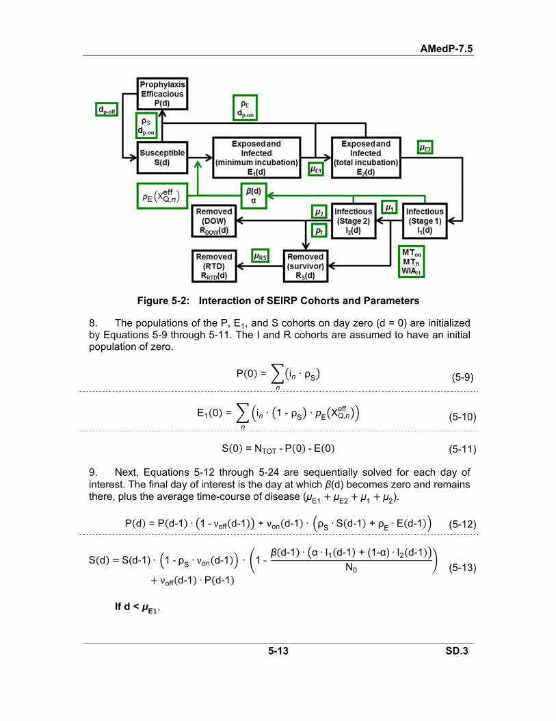
AMedP-7.5

5-13 SD.3

Figure 5-2: Interaction of SEIRP Cohorts and Parameters

8. The populations of the P, E1, and S cohorts on day zero (d = 0) are initialized by Equations 5-9 through 5-11. The I and R cohorts are assumed to have an initial population of zero.

P 0 = in · ρSn

(5-9)

E1 0 = in · 1 - ρS · pE XQ,neff

n

(5-10)

S 0 = NTOT - P 0 - E 0 (5-11)

9. Next, Equations 5-12 through 5-24 are sequentially solved for each day of interest. The final day of interest is the day at which β(d) becomes zero and remains there, plus the average time-course of disease (μE1 μE2 μ1 μ2).

P d = P d-1 · 1-νoff d-1 + νon d-1 · ρS · S d-1 + ρE ·E d-1 (5-12)

S d S(d-1)· 1-ρS·νon d-1 · 1 -β d-1 · α · I1 d-1 + (1-α) ·I2 d-1

N0

νoff d-1 ·P d-1 (5-13)

If d < μE1,

AMedP-7.5

5-14 SD.3

E1 d = E1 d-1 · 1 - ρE · νon d-1 (5-14)

E2 d = 0 (5-15)

If d = μE1,

E1 d = 0 (5-16)

E2 d = E1 d-1 · 1 - ρE · νon d-1 (5-17)

If d > μE1,

E1 d = E1 d-1 · 1 - ρE · νon d-1 · 1 - 1

μE1

S(d-1) · 1 - ρS · νon d-1 · β d-1 · α · I1 d-1 + (1-α) · I2 d-1

N0

(5-18)

E2 d = E2 d-1 · 1-ρE·νon d-1 · 1 -1

μE2

+E1 d-1 · 1 - ρE ·νon d-1

μE1

(5-19)

I1 d = I1 d-1 · 1-1

μ1

+E2 d-1 · 1-ρE·νon d-1

μE2

· 1 - MTon d ·MTI1·WIAI1 (5-20)

I2 d = I2 d-1 · 1 - 1

μ2

+I1 d-1

μ1

(5-21)

RDOW d = RDOW d-1 +I2 d-1

μ2

· pf d-1 (5-22)

AMedP-7.5

5-15 SD.3

RS d = RS d-1 + I2 d-1

μ2

· 1 - pf d-1 ‐I2 d- 1+μRS

μ2

· 1 - pf d-1

MTon d · MTI1 · WIAI1 ∙ I1 d-1 · 1 - 1

μ1

+E2 d-1 · 1 - ρE·νon d-1

μE2

MTon d-μRS · MTI1 · WIAI1

∙ I1 d- 1+μRS · 1 - 1

μ1

+ E2 d- 1+μRS · 1 - ρE·νon d- 1+μRS

μE2

(5-23)

RRTD d = RRTD d-1 + I2 d- 1+μRS

μ2

· 1 - pf d- 1+μRS

MTon d-μRS · MTI1 · WIAI1 · I1 d- 1+μRS · 1 - 1

μ1

E2 d- 1+μRS · 1 - ρE·νon d- 1+μRS

μE2

(5-24)

10. Finally, the cohort populations, calculated according to the preceding equations, Table 5-3 gives guidance on which equations should be used to populate the output tables for pneumonic plague and smallpox.

Table 5-3: Guidance on Using SEIRP Equations to Populate Output Tables

CAT Rate Table

CAT Personnel Status Table

Plague Smallpox Plague Smallpox

WIA WIA(1+) or WIA(2+): Eq. 5-25

WIA(3+): Eq. 5-26

WIA(1) None None WIA(2) Eq. 5-20 Eq. 5-20

WIA(3) None Eq. 5-27

WIA(4) Eq. 5-21 Eq. 5-28

DOW Eq. 5-29 Eq. 5-29 DOW Eq. 5-22 Eq. 5-22

CONV None Eq. 5-30 CONV None Eq. 5-23

RTD Eq. 5-31 Eq. 5-31 RTD Eq. 5-24 Eq. 5-24

I1,new d = E2 d-1 · 1 - ρE·νon d-1

μE2

· 1 - MTon d · MTI1 · WIAI1 (5-25)

AMedP-7.5

5-16 SD.3

I2,new d =I1 d-1

μ1

(5-26)

WIA(3)spox d = WIA(3)spox d-1 · 1 - 1

μ2

+ I2,new d · 1 - pf d-1 (5-27)

WIA(4)spox d = WIA(4)spox d-1 · 1 - 1

μ2

+ I2,new d · pf d-1 (5-28)

RDOW,new d = RDOW,new d ‐ RDOW,new d-1 (5-29)

RS,new d = I2 d-1

μ2

· 1 - pf d-1

MTon d · MTI1 · WIAI1 · I1 d-1 · 1 - 1

μ1

+E2 d-1 · 1 - ρE·νon d-1

μE2

(5-30)

RRTD,new d = RRTD,new d ‐RRTD,new d-1 (5-31)

11. Assumptions, limitations, and constraints.

a. Assumptions.

1) The population is large and unstructured.

2) The population mixes homogeneously.

3) Initial and transmission-caused infections follow the same course of disease.

4) The epidemiological circumstances of the historical outbreaks from which the time-varying rate of disease transmission (β(d)) was derived are similar to the circumstances in scenarios of interest to the user.

5) Individuals who enter become WIA, survive the illness (with or without medical treatment), and RTD gain immunity to the disease. Therefore, they do not re-enter the S cohort upon becoming RTD.

b. Limitation. The model does not account for medical treatment in any way. If the user sets FlagMT to Yes, the only difference in output is that survivors become RTD instead of remaining as WIA.

c. Constraints.

AMedP-7.5

5-17 SD.3

1) Because the model uses only mean times (and not standard deviations) to represent the lengths of the incubation period and each stage of illness, it represents all probability distributions as exponential distributions.

2) The model uses finite-difference equations instead of differential equations and integrals (this introduces some unknown degree of inaccuracy).

5.1.6. Equations Needed to Execute Casualty Estimates

1. The equations presented in this section are necessary to estimate pE XQ,neff and

pf XQ,neff , as required in Sections 5.1.4 and 5.1.5. As warranted, the agent submodel

summary tables in Section 5.2 will refer to these equations.

2. Most infectivity models and some lethality models use a lognormal distribution to calculate the probability of illness or of death. Equation 5-32 may be used to calculate the values of these lognormal distributions.

pE XQ,neff or pf XQ,n

eff = Φ PSQ · log10

XQ,neff

ID50,Q, ED50,Q, or LD50,Q (5-32)

where:

pE XQ,neff and pf XQ,n

eff are the cumulative fraction of individuals at icon n

who received Effective CBRN Challenge XQ,neff that will become ill (for

infectivity/effectivity), or that will die (for lethality),

Φ is the standard normal cumulative distribution function,

ID50,Q_k, ED50,Q_k, and LD50,Q_k are the ID50, ED50, and LD50, respectively, for challenge type Q (values are agent specific—see Section 5.2),

PS is the base 10 probit slope associated with the ID50, ED50, or LD50 (values are agent specific—see Section 5.2),

3. A few infectivity models also use a threshold model to calculate the probability of illness—see Equation 5-33.

pE XQ,n

eff = 1 for XQ,neff ≥ T, and

pE XQ,neff = 0 for XQ,n

eff < T, (5-33)

where:

XQ,neff is the Effective CBRN Challenge for challenge type Q and icon n,

pE XQ,neff is the probability that an individual who did not receive prophylaxis

and inhaled a dose of XQ,neff will become ill,

T is the threshold value (value is agent-specific).

AMedP-7.5

5-18 SD.3

4. The anthrax lethality model for individuals who receive antibiotic treatment uses a linear function to compute a time-dependent CFR—see Equation 5-34.

CFR dIn-Stg1 = m · dIn-Stg1 + b (5-34)

where:

CFR(d) is the case fatality rate [%],

dIn-Stg1 is the number of days since the individual entered stage 1 of illness [days],

m is the slope [%/day], and

b is the intercept [%].

5.2. BIOLOGICAL AGENT MODELS

5.2.1. Anthrax

1. Figure 5-3 summarizes the human response and casualty estimation processes for anthrax, Table 5-6 summarizes the Injury Profile, Table 5-8 summarizes the other anthrax submodels, and Table 5-7 summarizes the available anthrax prophylaxis options.

2. Assumptions and limitation.

a. Assumptions.

1) The disease resulting from exposure to B. anthracis is inhalation anthrax.

2) Untreated inhalation anthrax is 100% lethal.

b. Limitation. Although the model requires the user to specify a day on which antibiotic treatment becomes available (dtrt-anth), it does not apply treatment to every person on that day; only those who have been declared WIA are modeled to begin receiving antibiotics on that day. Those who are declared WIA after dtrt-anth are modeled to begin receiving antibiotics on the day they are declared WIA.

3. Cohorts and special considerations.

a. The incubation period of anthrax is dose-dependent. Thus, the cohorts are separated according to dose range, and the PDTs contain unique probability distributions for each dose range. Table 5-4 summarizes the dose ranges. The E cohort is split into sub-cohorts labeled as EDR, where DR is the dose range label given in Table 5-4. The population of each EDR is calculated separately for each dose range by applying Equation 5-1 to icons within the appropriate range of doses.

AMedP-7.5

5-19 SD.3

Table 5-4: Anthrax Dose Ranges Dose Range Label (DR) Dose Range (spores)*

A Xanth,neff ≤ 102

B 102 < Xanth,neff ≤ 103

C 103 < Xanth,neff ≤ 104

D 104 < Xanth,neff ≤ 105

E 105 < Xanth,neff ≤ 106

F 106 < Xanth,neff ≤ 107

G Xanth,neff > 107

* The values in the anthrax PDTs (Table 5-9 to Table 5-16) are calculated based on the upper dose for each dose range, with the exception of dose range G, which uses a dose of 2×107 spores.

b. If FlagMT = No, the populations of the EDR cohorts move to the FDR,U cohorts as individuals DOW. No SDR,U cohorts are used because the untreated lethality model is a 100% CFR (see Table 5-8).

c. If FlagMT = Yes, an individual’s duration of illness and outcome depend upon the day on which antibiotic treatment becomes available. The user must specify the day on which antibiotic treatment becomes available for those declared WIA (dtrt-anth). Based on dtrt-anth and the casualty criterion, the populations of the EDR sub-cohorts are split among several sub-cohorts, as specified below.

1) If the casualty criterion is WIA(1+) or WIA(2+), the EDR sub-cohorts are split among the following list of sub-cohorts, according to Equations 5-35 to 5-39.

a) FDR,U is the number of individuals in dose range DR who die before dtrt-anth.

b) FDR,T-2 is the number of individuals in dose range DR who are in Stage 2 on dtrt-anth, and will die despite antibiotic treatment.

c) FDR,T-1 is the number of individuals in dose range DR who are in Stage 1 on dtrt-anth, and will die despite antibiotic treatment.

d) SDR,T-1 is the number of individuals in dose range DR who are in Stage 1 on dtrt-anth, and will survive as a result of antibiotic treatment.

FDR,U = EDR · PDT5-11 d

dtrt-anth

d=1

(5-35)

FDR,T-2 = EDR · PDT5-10 d

dtrt-anth

d=1

- FDR,U (5-36)

AMedP-7.5

5-20 SD.3

FDR,T-1 = EDR· pf,T-1·PDT5-9 dStg1 ·Pin-Stg1

dtrt-anth

dStg1=1

+ 0.1· 1- PDT5-9 d

dtrt-anth

d=1

(5-37)

SDR,T-1 = EDR - FDR,U - FDR,T-2 - FDR,T-1 (5-38)

pf,T-1 = 0.012 · dtrt-anth - dStg1 + 0.1 (5-39)

In Equations 5-35 to 5-39:

dtrt-anth is the user-specified day on which treatment begins,

dStg1 is the day on which different fractions of EDR enter Stage 1,

(dtrt-anth-dStg1) is the number of days between the onset of symptoms and the beginning of antibiotic treatment.

PDT5-X d or dStg1 reflect fractions of a specific population that have entered a certain stage of disease, as a function of a chosen day (d or dStg1), as dictated by Table 5-X,

pf,T-1 is the probability of fatality for anthrax patients whose treatment is initiated in Stage 1,

Pin-Stg1 is the probability that an individual who entered Stage 1 of anthrax dtrt-anth-dStg1) days ago is still in Stage 1 (see Table 5-5).

2) If the casualty criterion is WIA(3+), the EDR sub-cohorts are split among the FDR,U and FDR,T-2 sub-cohorts, according to Equations 5-40 and 5-41

FDR,U = EDR · PDT5-11 d

dtrt-anth

d=1

(5-40)

FDR,T-2 = EDR - FDR,U (5-41)

AMedP-7.5

5-21 SD.3

Table 5-5: Probability of an Individual Still Being in Stage 1 of Anthrax (Pin-Stg1) After Specified Durations Spent in Stage 1

Days After Entering Stage 1

(dtrt-anth- dStg1)

Probability (Pin-Stg1)

Days After Entering Stage 1

(dtrt-anth - dStg1)

Probability(Pin-Stg1)

Days After Entering Stage 1

(dtrt-anth - dStg1)

Probability(Pin-Stg1)

0 1.0000 9 0.0407 18 0.0010 1 0.9946 10 0.0257 19 0.0007 2 0.8835 11 0.0164 20 0.0005 3 0.6558 12 0.0106 21 0.0004 4 0.4362 13 0.0069 22 0.0003 5 0.2755 14 0.0046 23 0.0002 6 0.1705 15 0.0031 24 0.00017 0.1051 16 0.0021 ≥25 0.0000 8 0.0651 17 0.0014

4. Table 5-9 through Table 5-16 are the PDTs for anthrax. The dose-bin specific values in a given table are to be used in Equations 5-5 through 5-8 with the cohort(s) listed in the table headers and footers, per Figure 5-3.

Table 5-6: Anthrax Injury Profile Stage Injury Severity Level

Untreated Non-Survivors (FDR,U)1 2 2 4

Stage 1 Treated Survivors (SDR,T-1) 1 2 2 4 3 3

CONV CONV Stage 1 (FDR,T-1) and Stage 2 (FDR,T-2) Treated Non-Survivors

1 2 2 4

Table 5-7: Anthrax Prophylaxis Summary Type of Prophylaxis Efficacy (ρn)

Pre-exposure vaccination or antibiotics 0.90 Pre-exposure vaccination and post-exposure antibiotics 1.00

Post-exposure vaccination and antibiotics 1.00

AMedP-7.5

5-22 SD.3

Table 5-8: Anthrax Submodel Summary Type Value

Infectivity (pE Xanth,neff )

Lognormal Distribution Use Equation 5-32

ID50 = 16,000 spores Probit slope = 0.79 probits/log(dose)

Lethality (pf anth ) Untreated OR Treatment Initiated in Stage 2

CFR 100% Treatment Initiated in Stage 1

Linear Function Use Equation 5-34 m = 0.012 %/day

b = 0.1 %

Incubation Period*

Dose-Dependent Lognormal Distribution

Dose Range Mean (days) Standard Deviation (days) A 9.36 6.74 B 7.34 4.52 C 5.52 2.86 D 3.86 1.65 E 2.32 0.79 F 0.88 0.22 G 0.46 0.10

Duration of Illness*

Stage 1: Untreated (FDR,U)

Stage 1: Treatment Initiated in Stage 2 (FDR,T-2)

Lognormal Distribution Mean = 4.2 days

Standard deviation = 2.3 days Stage 2: Untreated (FDR,U)

Lognormal Distribution Mean = 0.70 days

Standard deviation = 0.74 days Stage 1: Treatment Initiated in Stage 1 (SDR,T-1 and FDR,T-1)

Lognormal Distribution Mean = 5.8 days

Standard deviation = 2.0 days Stage 2: Treatment Initiated in Stage 1 (SDR,T-1 and FDR,T-1)

Lognormal Distribution Mean = 1.4 days

Standard deviation = 1.8 days Stage 3: Treatment Initiated in Stage 1 (SDR,T-1)

Constant 11 days CONV: Treatment Initiated in Stage 1 (SDR,T-1)

Constant 60 days Stage 2: Treatment Initiated in Stage 2 (FDR,T-2)

Lognormal Distribution Mean = 1.5 days

Standard deviation = 1.3 days * Presented for information only. These two submodels have already been convolved to generate the

PDTs; the user should use the PDTs to estimate when changes in casualty category occur.

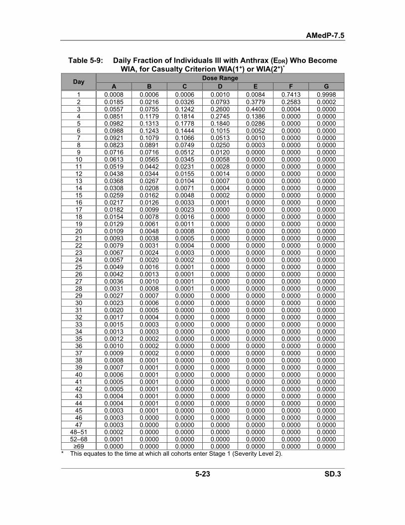
AMedP-7.5

5-23 SD.3

Table 5-9: Daily Fraction of Individuals Ill with Anthrax (EDR) Who Become WIA, for Casualty Criterion WIA(1+) or WIA(2+)*

Day Dose Range

A B C D E F G1 0.0008 0.0006 0.0006 0.0010 0.0084 0.7413 0.9998 2 0.0185 0.0216 0.0326 0.0793 0.3779 0.2583 0.00023 0.0557 0.0755 0.1242 0.2600 0.4400 0.0004 0.00004 0.0851 0.1179 0.1814 0.2745 0.1386 0.0000 0.00005 0.0982 0.1313 0.1778 0.1840 0.0286 0.0000 0.00006 0.0988 0.1243 0.1444 0.1015 0.0052 0.0000 0.00007 0.0921 0.1079 0.1066 0.0513 0.0010 0.0000 0.00008 0.0823 0.0891 0.0749 0.0250 0.0003 0.0000 0.00009 0.0716 0.0716 0.0512 0.0120 0.0000 0.0000 0.000010 0.0613 0.0565 0.0345 0.0058 0.0000 0.0000 0.000011 0.0519 0.0442 0.0231 0.0028 0.0000 0.0000 0.000012 0.0438 0.0344 0.0155 0.0014 0.0000 0.0000 0.000013 0.0368 0.0267 0.0104 0.0007 0.0000 0.0000 0.000014 0.0308 0.0208 0.0071 0.0004 0.0000 0.0000 0.000015 0.0259 0.0162 0.0048 0.0002 0.0000 0.0000 0.000016 0.0217 0.0126 0.0033 0.0001 0.0000 0.0000 0.000017 0.0182 0.0099 0.0023 0.0000 0.0000 0.0000 0.000018 0.0154 0.0078 0.0016 0.0000 0.0000 0.0000 0.000019 0.0129 0.0061 0.0011 0.0000 0.0000 0.0000 0.000020 0.0109 0.0048 0.0008 0.0000 0.0000 0.0000 0.000021 0.0093 0.0038 0.0005 0.0000 0.0000 0.0000 0.000022 0.0079 0.0031 0.0004 0.0000 0.0000 0.0000 0.000023 0.0067 0.0024 0.0003 0.0000 0.0000 0.0000 0.000024 0.0057 0.0020 0.0002 0.0000 0.0000 0.0000 0.000025 0.0049 0.0016 0.0001 0.0000 0.0000 0.0000 0.000026 0.0042 0.0013 0.0001 0.0000 0.0000 0.0000 0.000027 0.0036 0.0010 0.0001 0.0000 0.0000 0.0000 0.000028 0.0031 0.0008 0.0001 0.0000 0.0000 0.0000 0.000029 0.0027 0.0007 0.0000 0.0000 0.0000 0.0000 0.000030 0.0023 0.0006 0.0000 0.0000 0.0000 0.0000 0.000031 0.0020 0.0005 0.0000 0.0000 0.0000 0.0000 0.000032 0.0017 0.0004 0.0000 0.0000 0.0000 0.0000 0.000033 0.0015 0.0003 0.0000 0.0000 0.0000 0.0000 0.000034 0.0013 0.0003 0.0000 0.0000 0.0000 0.0000 0.000035 0.0012 0.0002 0.0000 0.0000 0.0000 0.0000 0.000036 0.0010 0.0002 0.0000 0.0000 0.0000 0.0000 0.000037 0.0009 0.0002 0.0000 0.0000 0.0000 0.0000 0.000038 0.0008 0.0001 0.0000 0.0000 0.0000 0.0000 0.000039 0.0007 0.0001 0.0000 0.0000 0.0000 0.0000 0.000040 0.0006 0.0001 0.0000 0.0000 0.0000 0.0000 0.000041 0.0005 0.0001 0.0000 0.0000 0.0000 0.0000 0.000042 0.0005 0.0001 0.0000 0.0000 0.0000 0.0000 0.000043 0.0004 0.0001 0.0000 0.0000 0.0000 0.0000 0.000044 0.0004 0.0001 0.0000 0.0000 0.0000 0.0000 0.000045 0.0003 0.0001 0.0000 0.0000 0.0000 0.0000 0.000046 0.0003 0.0000 0.0000 0.0000 0.0000 0.0000 0.000047 0.0003 0.0000 0.0000 0.0000 0.0000 0.0000 0.0000

48–51 0.0002 0.0000 0.0000 0.0000 0.0000 0.0000 0.000052–68 0.0001 0.0000 0.0000 0.0000 0.0000 0.0000 0.0000≥69 0.0000 0.0000 0.0000 0.0000 0.0000 0.0000 0.0000

* This equates to the time at which all cohorts enter Stage 1 (Severity Level 2).

AMedP-7.5

5-24 SD.3

Table 5-10: Daily Fraction of Individuals Ill with Anthrax (EDR) Who Become WIA, for Casualty Criterion WIA(3+)*

Day Dose Range

A B C D E F G

1 0.0000 0.0000 0.0000 0.0000 0.0000 0.0000 0.0002 2 0.0000 0.0000 0.0000 0.0000 0.0002 0.0132 0.0451 3 0.0007 0.0007 0.0010 0.0023 0.0134 0.1296 0.1889 4 0.0055 0.0066 0.0102 0.0236 0.0872 0.2290 0.23465 0.0179 0.0234 0.0373 0.0774 0.1803 0.2127 0.1893 6 0.0363 0.0489 0.0762 0.1358 0.2068 0.1537 0.1289 7 0.0554 0.0746 0.1101 0.1645 0.1738 0.0999 0.0817 8 0.0705 0.0929 0.1273 0.1585 0.1238 0.0621 0.0503 9 0.0794 0.1012 0.1272 0.1317 0.0810 0.0380 0.0307 10 0.0823 0.1005 0.1148 0.0994 0.0508 0.0232 0.0188 11 0.0805 0.0934 0.0966 0.0703 0.0313 0.0142 0.0115 12 0.0754 0.0829 0.0773 0.0477 0.0192 0.0088 0.0072 13 0.0686 0.0711 0.0596 0.0315 0.0118 0.0055 0.0045 14 0.0610 0.0594 0.0448 0.0204 0.0073 0.0035 0.0029 15 0.0534 0.0488 0.0330 0.0131 0.0046 0.0022 0.0018 16 0.0462 0.0396 0.0240 0.0084 0.0029 0.0014 0.0012 17 0.0396 0.0318 0.0173 0.0054 0.0019 0.0009 0.0008 18 0.0338 0.0254 0.0124 0.0034 0.0012 0.0006 0.0005 19 0.0287 0.0202 0.0088 0.0022 0.0008 0.0004 0.0004 20 0.0243 0.0160 0.0063 0.0014 0.0005 0.0003 0.0002 21 0.0206 0.0127 0.0045 0.0009 0.0004 0.0002 0.0002 22 0.0174 0.0100 0.0032 0.0006 0.0002 0.0001 0.0001 23 0.0147 0.0079 0.0023 0.0004 0.0002 0.0001 0.0001 24 0.0125 0.0063 0.0016 0.0003 0.0001 0.0001 0.0001 25 0.0106 0.0050 0.0012 0.0002 0.0001 0.0001 0.0000 26 0.0090 0.0040 0.0008 0.0001 0.0001 0.0001 0.0000 27 0.0076 0.0032 0.0006 0.0001 0.0001 0.0001 0.0000 28 0.0065 0.0025 0.0004 0.0001 0.0000 0.0000 0.0000 29 0.0055 0.0020 0.0003 0.0001 0.0000 0.0000 0.0000 30 0.0047 0.0016 0.0002 0.0001 0.0000 0.0000 0.0000 31 0.0041 0.0013 0.0002 0.0001 0.0000 0.0000 0.0000 32 0.0035 0.0011 0.0001 0.0000 0.0000 0.0000 0.0000 33 0.0030 0.0009 0.0001 0.0000 0.0000 0.0000 0.0000 34 0.0026 0.0007 0.0001 0.0000 0.0000 0.0000 0.0000 35 0.0022 0.0006 0.0001 0.0000 0.0000 0.0000 0.0000 36 0.0019 0.0005 0.0001 0.0000 0.0000 0.0000 0.0000 37 0.0017 0.0004 0.0000 0.0000 0.0000 0.0000 0.0000 38 0.0015 0.0003 0.0000 0.0000 0.0000 0.0000 0.0000 39 0.0013 0.0003 0.0000 0.0000 0.0000 0.0000 0.0000 40 0.0011 0.0002 0.0000 0.0000 0.0000 0.0000 0.0000 41 0.0010 0.0002 0.0000 0.0000 0.0000 0.0000 0.0000 42 0.0009 0.0002 0.0000 0.0000 0.0000 0.0000 0.0000 43 0.0008 0.0001 0.0000 0.0000 0.0000 0.0000 0.0000 44 0.0007 0.0001 0.0000 0.0000 0.0000 0.0000 0.0000 45 0.0006 0.0001 0.0000 0.0000 0.0000 0.0000 0.0000 46 0.0005 0.0001 0.0000 0.0000 0.0000 0.0000 0.0000 47 0.0005 0.0001 0.0000 0.0000 0.0000 0.0000 0.0000 48 0.0004 0.0001 0.0000 0.0000 0.0000 0.0000 0.0000 49 0.0004 0.0001 0.0000 0.0000 0.0000 0.0000 0.0000

AMedP-7.5

5-25 SD.3

Day Dose Range

A B C D E F G50–52 0.0003 0.0000 0.0000 0.0000 0.0000 0.0000 0.0000 53–56 0.0002 0.0000 0.0000 0.0000 0.0000 0.0000 0.0000 57–66 0.0001 0.0000 0.0000 0.0000 0.0000 0.0000 0.0000 ≥67 0.0000 0.0000 0.0000 0.0000 0.0000 0.0000 0.0000

* When the casualty criterion is WIA(3+), this equates to the time at which all casualties enter Stage 2 (Severity Level 4). When the casualty criterion is WIA(1+) or WIA(2+), this equates to the time at which the FDR,U and FDR,T-2 cohorts enter Stage 2 (Severity Level 4).

Table 5-11: Daily Fraction of Untreated Anthrax Non-Survivors (FDR,U) Who DOW

Day Dose Range

A B C D E F G

1 0.0000 0.0000 0.0000 0.0000 0.0000 0.0000 0.0000 2 0.0000 0.0000 0.0000 0.0000 0.0000 0.0022 0.0111 3 0.0002 0.0002 0.0002 0.0005 0.0034 0.0560 0.1048 4 0.0023 0.0026 0.0039 0.0092 0.0399 0.1701 0.2030 5 0.0099 0.0126 0.0199 0.0434 0.1233 0.2148 0.2091 6 0.0244 0.0325 0.0513 0.0985 0.1863 0.1851 0.1638 7 0.0427 0.0575 0.0874 0.1438 0.1890 0.1335 0.1127 8 0.0599 0.0799 0.1143 0.1589 0.1530 0.0884 0.0729 9 0.0726 0.0944 0.1252 0.1465 0.1089 0.0561 0.0458 10 0.0795 0.0997 0.1213 0.1195 0.0722 0.0350 0.0285 11 0.0809 0.0971 0.1077 0.0898 0.0461 0.0217 0.0177 12 0.0783 0.0893 0.0899 0.0637 0.0289 0.0135 0.0110 13 0.0729 0.0788 0.0717 0.0435 0.0180 0.0084 0.0069 14 0.0660 0.0673 0.0553 0.0289 0.0112 0.0053 0.0044 15 0.0586 0.0562 0.0416 0.0189 0.0070 0.0034 0.0028 16 0.0512 0.0462 0.0307 0.0123 0.0045 0.0022 0.0018 17 0.0442 0.0374 0.0224 0.0079 0.0028 0.0014 0.0012 18 0.0379 0.0301 0.0162 0.0051 0.0018 0.0009 0.0008 19 0.0324 0.0240 0.0116 0.0033 0.0012 0.0006 0.0005 20 0.0275 0.0191 0.0083 0.0021 0.0008 0.0004 0.0004 21 0.0233 0.0152 0.0059 0.0014 0.0005 0.0003 0.0002 22 0.0197 0.0120 0.0042 0.0009 0.0004 0.0002 0.0002 23 0.0167 0.0095 0.0030 0.0006 0.0002 0.0001 0.000124 0.0141 0.0076 0.0022 0.0004 0.0002 0.0001 0.0001 25 0.0120 0.0060 0.0015 0.0003 0.0001 0.0001 0.0001 26 0.0102 0.0048 0.0011 0.0002 0.0001 0.0001 0.0001 27 0.0086 0.0038 0.0008 0.0001 0.0001 0.0001 0.0000 28 0.0073 0.0030 0.0006 0.0001 0.0001 0.0000 0.0000 29 0.0063 0.0024 0.0004 0.0001 0.0000 0.0000 0.000030 0.0053 0.0019 0.0003 0.0001 0.0000 0.0000 0.0000 31 0.0046 0.0016 0.0002 0.0000 0.0000 0.0000 0.0000 32 0.0039 0.0013 0.0002 0.0000 0.0000 0.0000 0.0000 33 0.0034 0.0010 0.0001 0.0000 0.0000 0.0000 0.0000 34 0.0029 0.0008 0.0001 0.0000 0.0000 0.0000 0.0000 35 0.0025 0.0007 0.0001 0.0000 0.0000 0.0000 0.000036 0.0022 0.0006 0.0001 0.0000 0.0000 0.0000 0.0000 37 0.0019 0.0005 0.0001 0.0000 0.0000 0.0000 0.0000 38 0.0016 0.0004 0.0001 0.0000 0.0000 0.0000 0.0000

AMedP-7.5

5-26 SD.3

Day Dose Range

A B C D E F G39 0.0014 0.0003 0.0001 0.0000 0.0000 0.0000 0.0000 40 0.0012 0.0003 0.0000 0.0000 0.0000 0.0000 0.0000 41 0.0011 0.0002 0.0000 0.0000 0.0000 0.0000 0.0000 42 0.0009 0.0002 0.0000 0.0000 0.0000 0.0000 0.000043 0.0008 0.0001 0.0000 0.0000 0.0000 0.0000 0.0000 44 0.0007 0.0001 0.0000 0.0000 0.0000 0.0000 0.0000 45 0.0006 0.0001 0.0000 0.0000 0.0000 0.0000 0.0000 46 0.0006 0.0001 0.0000 0.0000 0.0000 0.0000 0.0000 47 0.0005 0.0001 0.0000 0.0000 0.0000 0.0000 0.0000 48 0.0004 0.0001 0.0000 0.0000 0.0000 0.0000 0.000049 0.0004 0.0001 0.0000 0.0000 0.0000 0.0000 0.0000 50 0.0003 0.0001 0.0000 0.0000 0.0000 0.0000 0.0000 51 0.0003 0.0001 0.0000 0.0000 0.0000 0.0000 0.0000 52 0.0003 0.0000 0.0000 0.0000 0.0000 0.0000 0.0000

53–57 0.0002 0.0000 0.0000 0.0000 0.0000 0.0000 0.0000 58–73 0.0001 0.0000 0.0000 0.0000 0.0000 0.0000 0.0000 ≥74 0.0000 0.0000 0.0000 0.0000 0.0000 0.0000 0.0000

* Table values were calculated using the upper dose specified in each column heading, with the exception of the last column, which used 2×107 spores; each column is to be used for the range of inhaled doses specified in the column heading.

Table 5-12: Daily Fraction of Stage 1 Treated Anthrax Non-Survivors (FDR,T-1) and Survivors (SDR,T-1) Who Enter Stage 2

Day Dose Range

A B C D E F G

1 0.0000 0.0000 0.0000 0.0000 0.0000 0.0000 0.0000 2 0.0000 0.0000 0.0000 0.0000 0.0000 0.0000 0.0001 3 0.0000 0.0000 0.0000 0.0000 0.0001 0.0031 0.0112 4 0.0002 0.0002 0.0000 0.0006 0.0035 0.0459 0.0852 5 0.0020 0.0023 0.0007 0.0080 0.0335 0.1495 0.1903 6 0.0086 0.0109 0.0053 0.0374 0.1088 0.2197 0.2252 7 0.0223 0.0295 0.0196 0.0905 0.1831 0.2084 0.1881 8 0.0410 0.0551 0.0455 0.1423 0.2032 0.1537 0.1286 9 0.0597 0.0798 0.0766 0.1665 0.1722 0.0977 0.0780 10 0.0742 0.0970 0.1030 0.1586 0.1220 0.0567 0.044011 0.0823 0.1040 0.1175 0.1303 0.0768 0.0311 0.0237 12 0.0842 0.1019 0.1186 0.0962 0.0447 0.0165 0.0125 13 0.0813 0.0934 0.1094 0.0656 0.0247 0.0086 0.0064 14 0.0753 0.0816 0.0942 0.0421 0.0132 0.0044 0.0033 15 0.0676 0.0689 0.0770 0.0259 0.0069 0.0023 0.0017 16 0.0594 0.0566 0.0605 0.0154 0.0036 0.0012 0.000917 0.0514 0.0457 0.0461 0.0090 0.0018 0.0006 0.0004 18 0.0440 0.0365 0.0344 0.0051 0.0009 0.0003 0.0002 19 0.0374 0.0289 0.0253 0.0029 0.0005 0.0002 0.0001 20 0.0316 0.0227 0.0184 0.0016 0.0003 0.0001 0.0001 21 0.0267 0.0178 0.0133 0.0009 0.0001 0.0000 0.0000 22 0.0225 0.0140 0.0096 0.0005 0.0001 0.0000 0.000023 0.0189 0.0110 0.0068 0.0003 0.0000 0.0000 0.0000 24 0.0160 0.0086 0.0049 0.0002 0.0000 0.0000 0.0000 25 0.0135 0.0068 0.0035 0.0001 0.0000 0.0000 0.0000

AMedP-7.5

5-27 SD.3

Day Dose Range

A B C D E F G26 0.0114 0.0053 0.0026 0.0000 0.0000 0.0000 0.0000 27 0.0096 0.0042 0.0019 0.0000 0.0000 0.0000 0.0000 28 0.0082 0.0034 0.0014 0.0000 0.0000 0.0000 0.0000 29 0.0069 0.0027 0.0010 0.0000 0.0000 0.0000 0.000030 0.0059 0.0021 0.0007 0.0000 0.0000 0.0000 0.0000 31 0.0050 0.0017 0.0006 0.0000 0.0000 0.0000 0.0000 32 0.0043 0.0014 0.0004 0.0000 0.0000 0.0000 0.0000 33 0.0037 0.0011 0.0003 0.0000 0.0000 0.0000 0.0000 34 0.0032 0.0009 0.0002 0.0000 0.0000 0.0000 0.0000 35 0.0027 0.0007 0.0002 0.0000 0.0000 0.0000 0.000036 0.0024 0.0006 0.0001 0.0000 0.0000 0.0000 0.0000 37 0.0021 0.0005 0.0001 0.0000 0.0000 0.0000 0.0000 38 0.0018 0.0004 0.0001 0.0000 0.0000 0.0000 0.0000 39 0.0015 0.0003 0.0001 0.0000 0.0000 0.0000 0.0000 40 0.0013 0.0003 0.0001 0.0000 0.0000 0.0000 0.0000 41 0.0012 0.0002 0.0000 0.0000 0.0000 0.0000 0.0000 42 0.0010 0.0002 0.0000 0.0000 0.0000 0.0000 0.0000 43 0.0009 0.0002 0.0000 0.0000 0.0000 0.0000 0.0000 44 0.0008 0.0001 0.0000 0.0000 0.0000 0.0000 0.0000 45 0.0007 0.0001 0.0000 0.0000 0.0000 0.0000 0.0000 46 0.0006 0.0001 0.0000 0.0000 0.0000 0.0000 0.0000 47 0.0005 0.0001 0.0000 0.0000 0.0000 0.0000 0.0000 48 0.0005 0.0001 0.0000 0.0000 0.0000 0.0000 0.0000 49 0.0004 0.0001 0.0000 0.0000 0.0000 0.0000 0.0000 50 0.0004 0.0000 0.0000 0.0000 0.0000 0.0000 0.0000

51–53 0.0003 0.0000 0.0000 0.0000 0.0000 0.0000 0.0000 54–58 0.0002 0.0000 0.0000 0.0000 0.0000 0.0000 0.0000 59–68 0.0001 0.0000 0.0000 0.0000 0.0000 0.0000 0.0000 ≥69 0.0000 0.0000 0.0000 0.0000 0.0000 0.0000 0.0000

Table 5-13: Daily Fraction of Stage 1 Treated Anthrax Non-Survivors (FDR,T-1) Who DOW*

Day Dose Range

A B C D E F G

≤2 0.0000 0.0000 0.0000 0.0000 0.0000 0.0000 0.0000 3 0.0000 0.0000 0.0000 0.0000 0.0000 0.0003 0.0014 4 0.0000 0.0000 0.0000 0.0001 0.0005 0.0099 0.0234 5 0.0005 0.0005 0.0007 0.0017 0.0082 0.0584 0.09036 0.0028 0.0034 0.0053 0.0120 0.0420 0.1348 0.1618 7 0.0096 0.0124 0.0196 0.0407 0.1031 0.1821 0.1873 8 0.0219 0.0291 0.0454 0.0845 0.1567 0.1790 0.1672 9 0.0380 0.0509 0.0766 0.1251 0.1737 0.1448 0.1273 10 0.0543 0.0721 0.1030 0.1460 0.1557 0.1038 0.0878 11 0.0675 0.0878 0.1175 0.1435 0.1209 0.0690 0.057012 0.0758 0.0956 0.1186 0.1243 0.0852 0.0438 0.0357 13 0.0791 0.0958 0.1094 0.0982 0.0564 0.0272 0.0221 14 0.0780 0.0903 0.0941 0.0724 0.0359 0.0167 0.0136 15 0.0737 0.0811 0.0769 0.0508 0.0224 0.0103 0.0084 16 0.0676 0.0704 0.0604 0.0344 0.0138 0.0065 0.0053 17 0.0605 0.0594 0.0461 0.0227 0.0086 0.0041 0.0034

AMedP-7.5

5-28 SD.3

Day Dose Range

A B C D E F G18 0.0532 0.0492 0.0344 0.0148 0.0054 0.0027 0.0022 19 0.0462 0.0402 0.0253 0.0096 0.0035 0.0018 0.0015 20 0.0398 0.0324 0.0184 0.0062 0.0023 0.0012 0.0010 21 0.0340 0.0260 0.0133 0.0040 0.0015 0.0009 0.000722 0.0290 0.0207 0.0095 0.0026 0.0010 0.0006 0.0005 23 0.0246 0.0165 0.0068 0.0018 0.0007 0.0004 0.0004 24 0.0209 0.0131 0.0049 0.0012 0.0005 0.0003 0.0003 25 0.0177 0.0104 0.0035 0.0008 0.0004 0.0003 0.0002 26 0.0150 0.0083 0.0026 0.0006 0.0003 0.0002 0.0002 27 0.0127 0.0066 0.0019 0.0004 0.0002 0.0002 0.000228 0.0108 0.0053 0.0014 0.0003 0.0002 0.0001 0.0002 29 0.0092 0.0042 0.0010 0.0002 0.0001 0.0001 0.0001 30 0.0078 0.0034 0.0007 0.0002 0.0001 0.0001 0.0001 31 0.0067 0.0027 0.0006 0.0001 0.0001 0.0001 0.0001 32 0.0057 0.0022 0.0004 0.0001 0.0001 0.0001 0.0001 33 0.0049 0.0018 0.0003 0.0001 0.0001 0.0001 0.0001 34 0.0042 0.0014 0.0002 0.0001 0.0001 0.0001 0.0001 35 0.0036 0.0012 0.0002 0.0001 0.0001 0.0000 0.0000 36 0.0031 0.0010 0.0001 0.0001 0.0001 0.0000 0.0000 37 0.0027 0.0008 0.0001 0.0001 0.0001 0.0000 0.0000 38 0.0023 0.0006 0.0001 0.0001 0.0000 0.0000 0.0000 39 0.0020 0.0005 0.0001 0.0001 0.0000 0.0000 0.0000 40 0.0017 0.0004 0.0001 0.0000 0.0000 0.0000 0.0000 41 0.0015 0.0004 0.0001 0.0000 0.0000 0.0000 0.0000 42 0.0013 0.0003 0.0001 0.0000 0.0000 0.0000 0.0000 43 0.0012 0.0003 0.0001 0.0000 0.0000 0.0000 0.0000 44 0.0010 0.0002 0.0001 0.0000 0.0000 0.0000 0.0000 45 0.0009 0.0002 0.0001 0.0000 0.0000 0.0000 0.0000 46 0.0008 0.0001 0.0000 0.0000 0.0000 0.0000 0.0000 47 0.0007 0.0001 0.0000 0.0000 0.0000 0.0000 0.0000 48 0.0006 0.0001 0.0000 0.0000 0.0000 0.0000 0.0000 49 0.0005 0.0001 0.0000 0.0000 0.0000 0.0000 0.0000 50 0.0005 0.0001 0.0000 0.0000 0.0000 0.0000 0.0000 51 0.0004 0.0001 0.0000 0.0000 0.0000 0.0000 0.0000 52 0.0004 0.0001 0.0000 0.0000 0.0000 0.0000 0.0000 53 0.0003 0.0001 0.0000 0.0000 0.0000 0.0000 0.0000 54 0.0003 0.0001 0.0000 0.0000 0.0000 0.0000 0.0000 55 0.0003 0.0000 0.0000 0.0000 0.0000 0.0000 0.0000

56–59 0.0002 0.0000 0.0000 0.0000 0.0000 0.0000 0.0000 60–73 0.0001 0.0000 0.0000 0.0000 0.0000 0.0000 0.0000 ≥74 0.0000 0.0000 0.0000 0.0000 0.0000 0.0000 0.0000

* This equates to the time at which the SDR,T-1 enter Stage 3 (Severity Level 3).

Table 5-14: Daily Fraction of Stage 1 Treated Anthrax Survivors (SDR,T-1) Who Become CONV*

Day Dose Range

A B C D E F G

≤13 0.0000 0.0000 0.0000 0.0000 0.0000 0.0000 0.0000 14 0.0000 0.0000 0.0000 0.0000 0.0000 0.0003 0.0014 15 0.0000 0.0000 0.0000 0.0001 0.0005 0.0099 0.0234

AMedP-7.5

5-29 SD.3

Day Dose Range

A B C D E F G16 0.0005 0.0005 0.0007 0.0017 0.0082 0.0584 0.0903 17 0.0028 0.0034 0.0053 0.0120 0.0420 0.1348 0.1618 18 0.0096 0.0124 0.0196 0.0407 0.1031 0.1821 0.1873 19 0.0219 0.0291 0.0454 0.0845 0.1567 0.1790 0.167220 0.0380 0.0509 0.0766 0.1251 0.1737 0.1448 0.1273 21 0.0543 0.0721 0.1030 0.1460 0.1557 0.1038 0.0878 22 0.0675 0.0878 0.1175 0.1435 0.1209 0.0690 0.0570 23 0.0758 0.0956 0.1186 0.1243 0.0852 0.0438 0.0357 24 0.0791 0.0958 0.1094 0.0982 0.0564 0.0272 0.0221 25 0.0780 0.0903 0.0941 0.0724 0.0359 0.0167 0.013626 0.0737 0.0811 0.0769 0.0508 0.0224 0.0103 0.0084 27 0.0676 0.0704 0.0604 0.0344 0.0138 0.0065 0.0053 28 0.0605 0.0594 0.0461 0.0227 0.0086 0.0041 0.0034 29 0.0532 0.0492 0.0344 0.0148 0.0054 0.0027 0.0022 30 0.0462 0.0402 0.0253 0.0096 0.0035 0.0018 0.0015 31 0.0398 0.0324 0.0184 0.0062 0.0023 0.0012 0.0010 32 0.0340 0.0260 0.0133 0.0040 0.0015 0.0009 0.0007 33 0.0290 0.0207 0.0095 0.0026 0.0010 0.0006 0.0005 34 0.0246 0.0165 0.0068 0.0018 0.0007 0.0004 0.0004 35 0.0209 0.0131 0.0049 0.0012 0.0005 0.0003 0.0003 36 0.0177 0.0104 0.0035 0.0008 0.0004 0.0003 0.0002 37 0.0150 0.0083 0.0026 0.0006 0.0003 0.0002 0.0002 38 0.0127 0.0066 0.0019 0.0004 0.0002 0.0002 0.0002 39 0.0108 0.0053 0.0014 0.0003 0.0002 0.0001 0.0002 40 0.0092 0.0042 0.0010 0.0002 0.0001 0.0001 0.0001 41 0.0078 0.0034 0.0007 0.0002 0.0001 0.0001 0.0001 42 0.0067 0.0027 0.0006 0.0001 0.0001 0.0001 0.0001 43 0.0057 0.0022 0.0004 0.0001 0.0001 0.0001 0.0001 44 0.0049 0.0018 0.0003 0.0001 0.0001 0.0001 0.0001 45 0.0042 0.0014 0.0002 0.0001 0.0001 0.0001 0.0001 46 0.0036 0.0012 0.0002 0.0001 0.0001 0.0000 0.0000 47 0.0031 0.0010 0.0001 0.0001 0.0001 0.0000 0.0000 48 0.0027 0.0008 0.0001 0.0001 0.0001 0.0000 0.0000 49 0.0023 0.0006 0.0001 0.0001 0.0000 0.0000 0.0000 50 0.0020 0.0005 0.0001 0.0001 0.0000 0.0000 0.0000 51 0.0017 0.0004 0.0001 0.0000 0.0000 0.0000 0.0000 52 0.0015 0.0004 0.0001 0.0000 0.0000 0.0000 0.0000 53 0.0013 0.0003 0.0001 0.0000 0.0000 0.0000 0.0000 54 0.0012 0.0003 0.0001 0.0000 0.0000 0.0000 0.0000 55 0.0010 0.0002 0.0001 0.0000 0.0000 0.0000 0.0000 56 0.0009 0.0002 0.0001 0.0000 0.0000 0.0000 0.0000 57 0.0008 0.0001 0.0000 0.0000 0.0000 0.0000 0.0000 58 0.0007 0.0001 0.0000 0.0000 0.0000 0.0000 0.0000 59 0.0006 0.0001 0.0000 0.0000 0.0000 0.0000 0.0000 60 0.0005 0.0001 0.0000 0.0000 0.0000 0.0000 0.0000 61 0.0005 0.0001 0.0000 0.0000 0.0000 0.0000 0.0000 62 0.0004 0.0001 0.0000 0.0000 0.0000 0.0000 0.0000 63 0.0004 0.0001 0.0000 0.0000 0.0000 0.0000 0.0000 64 0.0003 0.0001 0.0000 0.0000 0.0000 0.0000 0.0000 65 0.0003 0.0001 0.0000 0.0000 0.0000 0.0000 0.0000 66 0.0003 0.0000 0.0000 0.0000 0.0000 0.0000 0.0000

AMedP-7.5

5-30 SD.3

Day Dose Range

A B C D E F G67–70 0.0002 0.0000 0.0000 0.0000 0.0000 0.0000 0.0000 71–84 0.0001 0.0000 0.0000 0.0000 0.0000 0.0000 0.0000 ≥85 0.0000 0.0000 0.0000 0.0000 0.0000 0.0000 0.0000

* This equates to the time at which the SDR,T-1 enter Stage 4 (Severity Level 2).

Table 5-15: Daily Fraction of Stage 1 Treated Anthrax Survivors (SDR,T-1) Who Become RTD

Day Dose Range

A B C D E F G

≤73 0.0000 0.0000 0.0000 0.0000 0.0000 0.0000 0.0000 74 0.0000 0.0000 0.0000 0.0000 0.0000 0.0003 0.0014 75 0.0000 0.0000 0.0000 0.0001 0.0005 0.0099 0.0234 76 0.0005 0.0005 0.0007 0.0017 0.0082 0.0584 0.0903 77 0.0028 0.0034 0.0053 0.0120 0.0420 0.1348 0.1618 78 0.0096 0.0124 0.0196 0.0407 0.1031 0.1821 0.1873 79 0.0219 0.0291 0.0454 0.0845 0.1567 0.1790 0.1672 80 0.0380 0.0509 0.0766 0.1251 0.1737 0.1448 0.127381 0.0543 0.0721 0.1030 0.1460 0.1557 0.1038 0.0878 82 0.0675 0.0878 0.1175 0.1435 0.1209 0.0690 0.0570 83 0.0758 0.0956 0.1186 0.1243 0.0852 0.0438 0.0357 84 0.0791 0.0958 0.1094 0.0982 0.0564 0.0272 0.0221 85 0.0780 0.0903 0.0941 0.0724 0.0359 0.0167 0.0136 86 0.0737 0.0811 0.0769 0.0508 0.0224 0.0103 0.008487 0.0676 0.0704 0.0604 0.0344 0.0138 0.0065 0.0053 88 0.0605 0.0594 0.0461 0.0227 0.0086 0.0041 0.0034 89 0.0532 0.0492 0.0344 0.0148 0.0054 0.0027 0.0022 90 0.0462 0.0402 0.0253 0.0096 0.0035 0.0018 0.0015 91 0.0398 0.0324 0.0184 0.0062 0.0023 0.0012 0.0010 92 0.0340 0.0260 0.0133 0.0040 0.0015 0.0009 0.000793 0.0290 0.0207 0.0095 0.0026 0.0010 0.0006 0.0005 94 0.0246 0.0165 0.0068 0.0018 0.0007 0.0004 0.0004 95 0.0209 0.0131 0.0049 0.0012 0.0005 0.0003 0.0003 96 0.0177 0.0104 0.0035 0.0008 0.0004 0.0003 0.0002 97 0.0150 0.0083 0.0026 0.0006 0.0003 0.0002 0.0002 98 0.0127 0.0066 0.0019 0.0004 0.0002 0.0002 0.0002 99 0.0108 0.0053 0.0014 0.0003 0.0002 0.0001 0.0002 100 0.0092 0.0042 0.0010 0.0002 0.0001 0.0001 0.0001 101 0.0078 0.0034 0.0007 0.0002 0.0001 0.0001 0.0001 102 0.0067 0.0027 0.0006 0.0001 0.0001 0.0001 0.0001 103 0.0057 0.0022 0.0004 0.0001 0.0001 0.0001 0.0001 104 0.0049 0.0018 0.0003 0.0001 0.0001 0.0001 0.0001 105 0.0042 0.0014 0.0002 0.0001 0.0001 0.0001 0.0001 106 0.0036 0.0012 0.0002 0.0001 0.0001 0.0000 0.0000 107 0.0031 0.0010 0.0001 0.0001 0.0001 0.0000 0.0000 108 0.0027 0.0008 0.0001 0.0001 0.0001 0.0000 0.0000 109 0.0023 0.0006 0.0001 0.0001 0.0000 0.0000 0.0000 110 0.0020 0.0005 0.0001 0.0001 0.0000 0.0000 0.0000 111 0.0017 0.0004 0.0001 0.0000 0.0000 0.0000 0.0000 112 0.0015 0.0004 0.0001 0.0000 0.0000 0.0000 0.0000 113 0.0013 0.0003 0.0001 0.0000 0.0000 0.0000 0.0000

AMedP-7.5

5-31 SD.3

Day Dose Range

A B C D E F G114 0.0012 0.0003 0.0001 0.0000 0.0000 0.0000 0.0000 115 0.0010 0.0002 0.0001 0.0000 0.0000 0.0000 0.0000 116 0.0009 0.0002 0.0001 0.0000 0.0000 0.0000 0.0000 117 0.0008 0.0001 0.0000 0.0000 0.0000 0.0000 0.0000118 0.0007 0.0001 0.0000 0.0000 0.0000 0.0000 0.0000 119 0.0006 0.0001 0.0000 0.0000 0.0000 0.0000 0.0000 120 0.0005 0.0001 0.0000 0.0000 0.0000 0.0000 0.0000 121 0.0005 0.0001 0.0000 0.0000 0.0000 0.0000 0.0000 122 0.0004 0.0001 0.0000 0.0000 0.0000 0.0000 0.0000 123 0.0004 0.0001 0.0000 0.0000 0.0000 0.0000 0.0000124 0.0003 0.0001 0.0000 0.0000 0.0000 0.0000 0.0000 125 0.0003 0.0001 0.0000 0.0000 0.0000 0.0000 0.0000 126 0.0003 0.0000 0.0000 0.0000 0.0000 0.0000 0.0000

127–130 0.0002 0.0000 0.0000 0.0000 0.0000 0.0000 0.0000 131–144 0.0001 0.0000 0.0000 0.0000 0.0000 0.0000 0.0000 ≥145 0.0000 0.0000 0.0000 0.0000 0.0000 0.0000 0.0000

Table 5-16: Daily Fraction of Stage 2 Treated Anthrax Non-Survivors (FDR,T-2) Who DOW

Day Dose Ranges (spores)*

<102 102 < - <103 103 < - <104 104 < - <105 105 < - <106 106 < - <107 >107

1 0.0000 0.0000 0.0000 0.0000 0.0000 0.0000 0.0000 2 0.0000 0.0000 0.0000 0.0000 0.0000 0.0004 0.0027 3 0.0001 0.0000 0.0001 0.0001 0.0009 0.0212 0.0480 4 0.0009 0.0010 0.0015 0.0034 0.0166 0.1020 0.1408 5 0.0051 0.0063 0.0098 0.0220 0.0721 0.1768 0.1908 6 0.0150 0.0197 0.0312 0.0631 0.1416 0.1893 0.1803 7 0.0302 0.0405 0.0627 0.1108 0.1759 0.1592 0.1418 8 0.0472 0.0632 0.0933 0.1420 0.1667 0.1176 0.1010 9 0.0621 0.0819 0.1133 0.1476 0.1342 0.0810 0.0682 10 0.0726 0.0930 0.1194 0.1330 0.0978 0.0537 0.0447 11 0.0778 0.0961 0.1137 0.1085 0.0672 0.0349 0.0289 12 0.0785 0.0928 0.1006 0.0825 0.0445 0.0224 0.0185 13 0.0755 0.0851 0.0841 0.0597 0.0290 0.0144 0.0119 14 0.0703 0.0751 0.0676 0.0418 0.0187 0.0093 0.0077 15 0.0637 0.0644 0.0526 0.0285 0.0120 0.0060 0.0050 16 0.0566 0.0540 0.0400 0.0191 0.0078 0.0039 0.0032 17 0.0496 0.0445 0.0299 0.0127 0.0050 0.0026 0.002118 0.0430 0.0363 0.0221 0.0084 0.0033 0.0017 0.0014 19 0.0370 0.0293 0.0161 0.0055 0.0022 0.0011 0.0010 20 0.0316 0.0235 0.0117 0.0037 0.0014 0.0008 0.0006 21 0.0269 0.0188 0.0084 0.0024 0.0010 0.0005 0.0004 22 0.0229 0.0150 0.0061 0.0016 0.0006 0.0004 0.0003 23 0.0194 0.0119 0.0044 0.0011 0.0004 0.0002 0.000224 0.0164 0.0095 0.0031 0.0007 0.0003 0.0002 0.0001 25 0.0139 0.0075 0.0023 0.0005 0.0002 0.0001 0.0001 26 0.0118 0.0060 0.0016 0.0003 0.0001 0.0001 0.0001 27 0.0100 0.0048 0.0012 0.0002 0.0001 0.0001 0.0001 28 0.0085 0.0038 0.0008 0.0002 0.0001 0.0000 0.0000 29 0.0073 0.0030 0.0006 0.0001 0.0001 0.0000 0.0000

AMedP-7.5

5-32 SD.3

Day Dose Ranges (spores)*

<102 102 < - <103 103 < - <104 104 < - <105 105 < - <106 106 < - <107 >107

30 0.0062 0.0024 0.0004 0.0001 0.0001 0.0000 0.0000 31 0.0053 0.0020 0.0003 0.0001 0.0001 0.0000 0.0000 32 0.0045 0.0016 0.0002 0.0001 0.0000 0.0000 0.0000 33 0.0039 0.0013 0.0002 0.0001 0.0000 0.0000 0.000034 0.0033 0.0010 0.0001 0.0001 0.0000 0.0000 0.0000 35 0.0029 0.0008 0.0001 0.0000 0.0000 0.0000 0.0000 36 0.0025 0.0007 0.0001 0.0000 0.0000 0.0000 0.0000 37 0.0021 0.0006 0.0001 0.0000 0.0000 0.0000 0.0000 38 0.0019 0.0005 0.0001 0.0000 0.0000 0.0000 0.0000 39 0.0016 0.0004 0.0001 0.0000 0.0000 0.0000 0.000040 0.0014 0.0003 0.0001 0.0000 0.0000 0.0000 0.0000 41 0.0012 0.0003 0.0000 0.0000 0.0000 0.0000 0.0000 42 0.0011 0.0002 0.0000 0.0000 0.0000 0.0000 0.0000 43 0.0009 0.0002 0.0000 0.0000 0.0000 0.0000 0.0000 44 0.0008 0.0001 0.0000 0.0000 0.0000 0.0000 0.0000 45 0.0007 0.0001 0.0000 0.0000 0.0000 0.0000 0.0000 46 0.0006 0.0001 0.0000 0.0000 0.0000 0.0000 0.0000 47 0.0006 0.0001 0.0000 0.0000 0.0000 0.0000 0.0000 48 0.0005 0.0001 0.0000 0.0000 0.0000 0.0000 0.0000 49 0.0004 0.0001 0.0000 0.0000 0.0000 0.0000 0.0000 50 0.0004 0.0001 0.0000 0.0000 0.0000 0.0000 0.0000

51–53 0.0003 0.0000 0.0000 0.0000 0.0000 0.0000 0.0000 54–58 0.0002 0.0000 0.0000 0.0000 0.0000 0.0000 0.0000 59–72 0.0001 0.0000 0.0000 0.0000 0.0000 0.0000 0.0000 ≥73 0.0000 0.0000 0.0000 0.0000 0.0000 0.0000 0.0000

AMedP-7.5

5-33 SD.3

Figure 5-3: Human Response and Casualty Estimation for Anthrax

5.2.2. Brucellosis

1. Figure 5-4 summarizes the human response and casualty estimation processes for brucellosis, Table 5-17 summarizes the Injury Profile, and Table 5-18 summarizes the other brucellosis submodels. No prophylaxis is modeled for brucellosis.

2. Assumptions, limitation, and constraint.

a. Assumptions.

1) The presentation and duration of brucellosis symptoms are independent of

AMedP-7.5

5-34 SD.3

the route of exposure.

2) Half of all cases are “abrupt,” and the other half are “insidious.”

3) One organism, one cell, and one CFU are equivalent.

4) Those who receive treatment will have a four week CONV period after their symptoms end (this period is reflected in the PDTs), before RTD.

b. Limitation. Although the model requires the user to specify a day on which antibiotic treatment becomes available (dtrt-bruc), it does not apply treatment to every person on that day; only those who have been declared WIA are modeled to begin receiving antibiotics on that day. Those who are declared WIA after dtrt-bruc are modeled to begin receiving antibiotics on the day they are declared WIA.

c. Constraint. The models apply to B. abortus, B. melitensis, and B. suis.

3. Cohorts and special considerations.

a. Brucellosis does not cause any fatalities, so no F cohort is used.

b. Brucellosis has two distinct clinical presentations, “abrupt” and “insidious” onset. Abrupt onset is immediately Severe, while insidious onset is first Mild, then Severe. The survivor cohorts are split between abrupt and insidious onset according to the assumption stated above.

c. If FlagMT = Yes, an individual’s duration of illness depends upon the day on which antibiotic treatment becomes available. The user must specify the day on which antibiotic treatment becomes available for those declared WIA (dtrt-bruc); based on the specified value, the population of E is split among several cohorts. Definitions of the cohorts and equations to calculate their populations are given below.

1) Sabr,U is the number of individuals with abrupt onset who recover and RTD before dtrt-bruc.

2) Sabr,T-WIA is the number of individuals with abrupt onset who are not yet WIA on dtrt-bruc, but will become WIA later and will receive antibiotic treatment when they become WIA.

3) Sabr,T is the number of individuals with abrupt onset who in Stage 1 on dtrt-bruc, and begin receiving antibiotic treatment that day.

4) Sins,U is the number of individuals with insidious onset who recover and RTD before dtrt-bruc.

5) Sins,T-WIA is the number of individuals with insidious onset who are not yet

AMedP-7.5

5-35 SD.3

WIA on dtrt-bruc, but will become WIA later and will receive antibiotic treatment when they become WIA.

6) Sins,T-1 is the number of individuals with insidious onset who are in Stage 1 on dtrt-bruc, and begin receiving antibiotic treatment that day.

7) Sins,T-2 is the number of individuals with insidious onset who are in Stage 2 on dtrt-bruc, and begin receiving antibiotic treatment that day.

Sabr,U = 0.5 · E · PDT5-21 d

dtrt-bruc

d=1

(5-42)

Sabr,T-WIA = 0.5 · E · 1 - PDT5-20 d

dtrt-bruc-1

d=1

(5-43)

Sabr,T = 0.5 · E - Sabr,U + Sabr,T-WIA (5-44)

Sins,U = 0.5 · E · PDT5-21 d

dtrt-bruc

d=1

(5-45)

Sins,T-WIA = 0.5 · E · 1 - PDT5-19 d

dtrt-bruc-1

d=1

(5-46)

8) If the casualty criterion is WIA(1+):

Sins,T-2 = 0.5 · E · PDT5-20 d

dtrt-bruc

d=1

- Sins,U (5-47)

Sins,T-1 = 0.5 · E - Sins,U + Sins,T-WIA + Sins,T-2 (5-48)

9) If the casualty criterion is WIA(2+) or WIA(3+):

Sins,T-2 = 0.5 · E - Sins,U + Sins,T-WIA (5-49)

Sins,T-1 = 0 (5-50)

In Equations 5-42 to 5-50:

dtrt-bruc is the user-specified day on which treatment begins, and

PDT5-X d reflect fractions of a specific population that have entered a certain stage of disease, as a function of a chosen day (d), as dictated

AMedP-7.5

5-36 SD.3

by Table 5-X.

4. Table 5-19 through Table 5-25 are the PDTs for brucellosis. The values from a given table are to be used in Equations 5-5 through 5-8 with the cohort(s) listed in the table headers and footers, per Figure 5-4.

Table 5-17: Brucellosis Injury Profile Stage Injury Severity Level

Abrupt Onset Brucellosis (Sabr,U, Sabr,T-WIA, Sabr,T) 1 3

Insidious Onset Brucellosis (Sins,U, Sins,T-WIA, Sins,T) 1 12 3

All Casualties Receiving Treatment (Sabr,T-WIA, Sabr,T, Sins,T-WIA, Sins,T) CONV CONV

Table 5-18: Brucellosis Submodel Summary Type Value

Infectivity (pE Xbruc,neff )

Lognormal Distribution Use Equation 5-32

ID50 = 949 organisms Probit slope = 2.58 probits/log(dose)

Lethality (pf bruc ) CFR 0%

Incubation Period*

Weibull Distribution Mean = 63.63 days

Standard deviation = 38.15 days

Duration of Illness*

Total Duration: All Untreated (Sabr,U, Sins,U)

Gamma Distribution Mean = 70.7 days

Standard deviation = 35.35 days Stage 1: Insidious Onset, Untreated (Sins,U) or Treatment Initiated in Stage 2 (Sins,T-2)

Gamma Distribution Mean = 30.87 days

Standard deviation = 33.88 days Stage 2: Insidious Onset, Untreated (Sins,U)

Difference between (Total Duration, Untreated) and (Stage 1, Insidious Onset, Untreated) Total Duration: All, Treatment Initiated Upon Becoming WIA (Sabr,T-WIA, Sins,T-WIA)

Constant 14 days

Total Duration: All, Treatment Initiated in Stage 1 or Stage 2 (Sabr,T, Sins,T-1, Sins,T-2) Constant 14 days after dtrt-bruc

CONV: All, Treatment at Any Point (Sabr,T-WIA, Sabr,T, Sins,T-WIA, Sins,T) Constant 28 days after end of symptoms

* Presented for information only. These two submodels have already been convolved to generate the PDTs; the user should use the PDTs to estimate when changes in casualty category occur.

AMedP-7.5

5-37 SD.3

Table 5-19: Daily Fraction of Individuals Ill with Insidious Onset Brucellosis (Sins,U, Sins,T-WIA, Sins,T-1, Sins,T-2) Who Become WIA, for Casualty Criterion WIA(1+);

Daily Fraction of Individuals Ill with Abrupt Onset Brucellosis (Sabr,U, Sabr,T-WIA, Sabr,T) Who Become WIA, for any Casualty Criterion*

Day Fraction Day Fraction Day Fraction Day Fraction Day Fraction1 0.0006 29 0.0101 72 0.0088 100 0.0052 130 0.0023 2 0.0015 30 0.0103 73 0.0087 101 0.0051 131 0.0022 3 0.0021 31 0.0104 74 0.0086 102 0.0050 132–133 0.0021 4 0.0027 32 0.0105 75 0.0085 103 0.0049 134 0.0020 5 0.0033 33 0.0106 76 0.0083 104 0.0047 135–136 0.0019 6 0.0038 34–35 0.0107 77 0.0082 105 0.0046 137–138 0.0018 7 0.0042 36 0.0108 78 0.0081 106 0.0045 139 0.0017 8 0.0047 37–39 0.0109 79 0.0079 107 0.0044 140–141 0.00169 0.0051 40–47 0.0110 80 0.0078 108 0.0043 142–143 0.0015

10 0.0055 48–50 0.0109 81 0.0077 109 0.0042 144–145 0.0014 11 0.0058 51–52 0.0108 82 0.0075 110 0.0041 146–147 0.0013 12 0.0062 53–54 0.0107 83 0.0074 111 0.0040 148–150 0.0012 13 0.0065 55 0.0106 84 0.0073 112 0.0039 151–152 0.0011 14 0.0069 56 0.0105 85 0.0071 113 0.0038 153–155 0.001015 0.0072 57–58 0.0104 86 0.0070 114 0.0037 156–158 0.0009 16 0.0075 59 0.0103 87 0.0069 115 0.0036 159–161 0.0008 17 0.0077 60 0.0102 88 0.0067 116 0.0035 162–165 0.0007 18 0.0080 61 0.0101 89 0.0066 117 0.0034 166–169 0.0006 19 0.0083 62 0.0100 90 0.0065 118 0.0033 170–174 0.0005 20 0.0085 63 0.0099 91 0.0064 119 0.0032 175–180 0.000421 0.0087 64 0.0098 92 0.0062 120 0.0031 181–188 0.0003 22 0.0089 65 0.0097 93 0.0061 121 0.0030 189–199 0.0002 23 0.0091 66 0.0096 94 0.0060 122 0.0029 200–221 0.0001 24 0.0093 67 0.0094 95 0.0058 123 0.0028 ≥222 0.0000 25 0.0095 68 0.0093 96 0.0057 124–125 0.0027 26 0.0097 69 0.0092 97 0.0056 126 0.0026 27 0.0098 70 0.0091 98 0.0055 127 0.0025 28 0.0100 71 0.0090 99 0.0053 128–129 0.0024

* This equates to the time at which all cohorts enter Stage 1 (Severity Level 3 for abrupt onset, and Severity Level 1 for insidious onset).

Table 5-20: Daily Fraction of Individuals Ill with Insidious Onset Brucellosis (Sins,U, Sins,T-2) Who Become WIA, for Casualty Criterion WIA(2+) or WIA(3+)*

Day Fraction Day Fraction Day Fraction Day Fraction Day Fraction1 0.0000 31 0.0050 67–76 0.0086 119–120 0.0057 157–158 0.0028

2–3 0.0001 32 0.0052 77–80 0.0085 121 0.0056 159–160 0.0027 4 0.0002 33 0.0054 81–82 0.0084 122 0.0055 161 0.0026 5 0.0004 34 0.0055 83–85 0.0083 123 0.0054 162–163 0.00256 0.0005 35 0.0057 86–87 0.0082 124 0.0053 164–165 0.0024 7 0.0006 36 0.0058 88–89 0.0081 125 0.0052 166–167 0.0023 8 0.0008 37 0.0060 90 0.0080 126–127 0.0051 168–169 0.0022 9 0.0009 38 0.0062 91–92 0.0079 128 0.0050 170–171 0.0021

10 0.0011 39 0.0063 93–94 0.0078 129 0.0049 172–173 0.0020 11 0.0013 40 0.0064 95 0.0077 130 0.0048 174–175 0.001912 0.0014 41 0.0066 96 0.0076 131 0.0047 175–178 0.0018 13 0.0016 42 0.0067 97–98 0.0075 132–133 0.0046 179–180 0.0017 14 0.0018 43 0.0069 99 0.0074 134 0.0045 181–183 0.0016

AMedP-7.5

5-38 SD.3

Day Fraction Day Fraction Day Fraction Day Fraction Day Fraction15 0.0020 44 0.0070 100 0.0073 135 0.0044 184–185 0.0015 16 0.0022 45 0.0071 101–102 0.0072 136 0.0043 186–188 0.0014 17 0.0024 46 0.0072 103 0.0071 137–138 0.0042 189–191 0.0013 18 0.0026 47 0.0073 104 0.0070 139 0.0041 192–195 0.0012 19 0.0028 48 0.0074 105–106 0.0069 140 0.0040 196–198 0.0011 20 0.0029 49 0.0075 107 0.0068 141–142 0.0039 199–202 0.0010 21 0.0031 50 0.0076 108 0.0067 143 0.0038 203–206 0.0009 22 0.0033 51 0.0077 109 0.0066 144 0.0037 207–211 0.0008 23 0.0035 52 0.0078 110 0.0065 145–146 0.0036 212–217 0.0007 24 0.0037 53 0.0079 111–112 0.0064 147 0.0035 218–223 0.0006 25 0.0039 54 0.0080 113 0.0063 148–149 0.0034 224–230 0.0005 26 0.0041 55–56 0.0081 114 0.0062 150 0.0033 231–240 0.0004 27 0.0043 57–58 0.0082 115 0.0061 151–152 0.0032 241–252 0.0003 28 0.0045 59–60 0.0083 116 0.0060 153 0.0031 253–269 0.0002 29 0.0047 61–62 0.0084 117 0.0059 154–155 0.0030 270–318 0.0001 30 0.0048 63–66 0.0085 118 0.0058 156 0.0029 ≥319 0.0000

* This equates to the time at which the Sins,U and Sins,T-2 cohorts enter Stage 2 (Severity Level 3).

Table 5-21: Daily Fraction of Untreated Insidious Onset Brucellosis Survivors (Sins,U) or Abrupt Onset Brucellosis Survivors (Sabr,U) Who Become RTD*

Day Fraction Day Fraction Day Fraction Day Fraction Day Fraction1–17 0.0000 61 0.0033 92 0.0069 157 0.0061 199 0.0030 18–23 0.0001 62 0.0035 93 0.0070 158 0.0060 200 0.0029 24–26 0.0002 63 0.0036 94 0.0071 159–160 0.0059 202–203 0.0028 27–29 0.0003 64 0.0037 95 0.0072 161 0.0058 204 0.0027 30–31 0.0004 65 0.0039 96 0.0072 162 0.0057 205–206 0.0026 32–33 0.0005 66 0.0040 97 0.0073 163 0.0056 207–208 0.0025

34 0.0006 67 0.0041 98 0.0074 164–165 0.0055 209–210 0.0024 35–36 0.0007 68 0.0042 99 0.0074 166 0.0054 211 0.0023

37 0.0008 69 0.0044 100 0.0075 167 0.0053 212–213 0.0022 38–39 0.0009 70 0.0045 101 0.0075 168–169 0.0052 214–215 0.0021

40 0.0010 71 0.0046 102–103 0.0076 170 0.0051 216–217 0.0020 41 0.0011 72 0.0048 104–106 0.0077 171 0.0050 219–220 0.0019 42 0.0012 73 0.0049 107–109 0.0078 172 0.0049 221–222 0.0018 43 0.0013 74 0.0050 110–124 0.0079 173–174 0.0048 223–224 0.0017 44 0.0014 75 0.0051 125–128 0.0078 175 0.0047 225–227 0.0016 45 0.0015 76 0.0053 129–131 0.0077 176 0.0046 228–229 0.0015 46 0.0016 77 0.0054 132–133 0.0076 177–178 0.0045 230–232 0.0014 47 0.0017 78 0.0055 134–135 0.0075 179 0.0044 233–235 0.0013 48 0.0018 79 0.0056 136–137 0.0074 180 0.0043 236–238 0.0012 49 0.0019 80 0.0057 138–139 0.0073 181–182 0.0042 239–241 0.0011 50 0.0020 81 0.0059 140–141 0.0072 183 0.0041 242–245 0.0010 51 0.0021 82 0.0060 142–143 0.0071 184 0.0040 246–249 0.0009 52 0.0022 83 0.0061 144 0.0070 185–186 0.0039 250–253 0.0008 53 0.0023 84 0.0062 145–146 0.0069 187 0.0038 254–258 0.0007 54 0.0025 85 0.0063 147 0.0068 188–189 0.0037 259–264 0.0006 55 0.0026 86 0.0064 148–149 0.0067 190 0.0036 265–270 0.0005 56 0.0027 87 0.0065 150 0.0066 191–192 0.0035 271–278 0.0004 57 0.0028 88 0.0066 151–152 0.0065 193 0.0034 279–289 0.0003 58 0.0030 89 0.0067 153 0.0064 194–194 0.0033 290–304 0.0002 59 0.0031 90 0.0068 154 0.0063 196 0.0032 305–334 0.0001 60 0.0032 91 0.0068 155–156 0.0062 197–198 0.0031 ≥335 0.0000

AMedP-7.5

5-39 SD.3

Table 5-22: Daily Fraction of Abrupt Onset Brucellosis Casualties Treated Upon Becoming WIA (Sabr,T-WIA) Who Become CONV*;

Daily Fraction of Insidious Onset Brucellosis Casualties Treated Upon Becoming WIA (Sins,T-WIA) Who Become CONV, for Casualty Criterion WIA(1+)* Day Fraction Day Fraction Day Fraction Day Fraction15 0.0006 / Xnorm 50 0.0108 / Xnorm 98 0.0073 / Xnorm 132 0.0033 / Xnorm

16 0.0015 / Xnorm 51–53 0.0109 / Xnorm 99 0.0071 / Xnorm 133 0.0032 / Xnorm

17 0.0021 / Xnorm 54–61 0.0110 / Xnorm 100 0.0070 / Xnorm 134 0.0031 / Xnorm

18 0.0027 / Xnorm 62–64 0.0109 / Xnorm 101 0.0069 / Xnorm 135 0.0030 / Xnorm

19 0.0033 / Xnorm 65–66 0.0108 / Xnorm 102 0.0067 / Xnorm 136 0.0029 / Xnorm

20 0.0038 / Xnorm 67–68 0.0107 / Xnorm 103 0.0066 / Xnorm 137 0.0028 / Xnorm

21 0.0042 / Xnorm 69 0.0106 / Xnorm 104 0.0065 / Xnorm 138–139 0.0027 / Xnorm

22 0.0047 / Xnorm 70 0.0105 / Xnorm 105 0.0064 / Xnorm 140 0.0026 / Xnorm

23 0.0051 / Xnorm 71–72 0.0104 / Xnorm 106 0.0062 / Xnorm 141 0.0025 / Xnorm

24 0.0055 / Xnorm 73 0.0103 / Xnorm 107 0.0061 / Xnorm 142–143 0.0024 / Xnorm

25 0.0058 / Xnorm 74 0.0102 / Xnorm 108 0.0060 / Xnorm 144 0.0023 / Xnorm

26 0.0062 / Xnorm 75 0.0101 / Xnorm 109 0.0058 / Xnorm 145 0.0022 / Xnorm

27 0.0065 / Xnorm 76 0.0100 / Xnorm 110 0.0057 / Xnorm 146–147 0.0021 / Xnorm

28 0.0069 / Xnorm 77 0.0099 / Xnorm 111 0.0056 / Xnorm 148 0.0020 / Xnorm

29 0.0072 / Xnorm 78 0.0098 / Xnorm 112 0.0055 / Xnorm 149–150 0.0019 / Xnorm

30 0.0075 / Xnorm 79 0.0097 / Xnorm 113 0.0053 / Xnorm 151–152 0.0018 / Xnorm

31 0.0077 / Xnorm 80 0.0096 / Xnorm 114 0.0052 / Xnorm 153 0.0017 / Xnorm

32 0.0080 / Xnorm 81 0.0094 / Xnorm 115 0.0051 / Xnorm 154–155 0.0016 / Xnorm

33 0.0083 / Xnorm 82 0.0093 / Xnorm 116 0.0050 / Xnorm 156–167 0.0015 / Xnorm

34 0.0085 / Xnorm 83 0.0092 / Xnorm 117 0.0049 / Xnorm 158–159 0.0014 / Xnorm

35 0.0087 / Xnorm 84 0.0091 / Xnorm 118 0.0047 / Xnorm 160–161 0.0013 / Xnorm

36 0.0089 / Xnorm 85 0.0090 / Xnorm 119 0.0046 / Xnorm 162–164 0.0012 / Xnorm

37 0.0091 / Xnorm 86 0.0088 / Xnorm 120 0.0045 / Xnorm 165–166 0.0011 / Xnorm

38 0.0093 / Xnorm 87 0.0087 / Xnorm 121 0.0044 / Xnorm 167–169 0.0010 / Xnorm

39 0.0095 / Xnorm 88 0.0086 / Xnorm 122 0.0043 / Xnorm 170–172 0.0009 / Xnorm

40 0.0097 / Xnorm 89 0.0085 / Xnorm 123 0.0042 / Xnorm 173–175 0.0008 / Xnorm

41 0.0098 / Xnorm 90 0.0083 / Xnorm 124 0.0041 / Xnorm 176–179 0.0007 / Xnorm

42 0.0100 / Xnorm 91 0.0082 / Xnorm 125 0.0040 / Xnorm 180–183 0.0006 / Xnorm

43 0.0101 / Xnorm 92 0.0081 / Xnorm 126 0.0039 / Xnorm 184–188 0.0005 / Xnorm

44 0.0103 / Xnorm 93 0.0079 / Xnorm 127 0.0038 / Xnorm 189–194 0.0004 / Xnorm

45 0.0104 / Xnorm 94 0.0078 / Xnorm 128 0.0037 / Xnorm 195–202 0.0003 / Xnorm

46 0.0105 / Xnorm 95 0.0077 / Xnorm 129 0.0036 / Xnorm 203–213 0.0002 / Xnorm

47 0.0106 / Xnorm 96 0.0075 / Xnorm 130 0.0035 / Xnorm 214–235 0.0001 / Xnorm

48–49 0.0107 / Xnorm 97 0.0074 / Xnorm 131 0.0034 / Xnorm ≥236 0.0000 * This equates to the time at which these cohorts exit their final stage of disease. This table is only

used for day > (14 + dtrt-bruc). Accordingly, Xnorm = ∑ PDT5-19 d221dtrt-bruc

.

Table 5-23: Daily Fraction of Insidious Onset Brucellosis Casualties Treated Upon Becoming WIA (Sins,T-WIA) Who Become CONV,

for Casualty Criterion WIA(2+) or WIA(3+)* Day Fraction Day Fraction Day Fraction Day Fraction≤15 0.0000 53 0.0063 / Xnorm 118 0.0070 / Xnorm 164 0.0033 / Xnorm

16–17 0.0001 / Xnorm 54 0.0064 / Xnorm 119–120 0.0069 / Xnorm 165–166 0.0032 / Xnorm

18 0.0002 / Xnorm 55 0.0066 / Xnorm 121 0.0068 / Xnorm 167 0.0031 / Xnorm

19 0.0004 / Xnorm 56 0.0067 / Xnorm 122 0.0067 / Xnorm 168–169 0.0030 / Xnorm

20 0.0005 / Xnorm 57 0.0069 / Xnorm 123 0.0066 / Xnorm 170 0.0029 / Xnorm

21 0.0006 / Xnorm 58 0.0070 / Xnorm 124 0.0065 / Xnorm 171–172 0.0028 / Xnorm

AMedP-7.5

5-40 SD.3

Day Fraction Day Fraction Day Fraction Day Fraction22 0.0008 / Xnorm 59 0.0071 / Xnorm 125–126 0.0064 / Xnorm 173–174 0.0027 / Xnorm

23 0.0009 / Xnorm 60 0.0072 / Xnorm 127 0.0063 / Xnorm 175 0.0026 / Xnorm

24 0.0011 / Xnorm 61 0.0073 / Xnorm 128 0.0062 / Xnorm 176–177 0.0025 / Xnorm

25 0.0013 / Xnorm 62 0.0074 / Xnorm 129 0.0061 / Xnorm 178–179 0.0024 / Xnorm

26 0.0014 / Xnorm 63 0.0075 / Xnorm 130 0.0060 / Xnorm 180–181 0.0023 / Xnorm

27 0.0016 / Xnorm 64 0.0076 / Xnorm 131 0.0059 / Xnorm 182–183 0.0022 / Xnorm

28 0.0018 / Xnorm 65 0.0077 / Xnorm 132 0.0058 / Xnorm 184–185 0.0021 / Xnorm

29 0.0020 / Xnorm 66 0.0078 / Xnorm 133–134 0.0057 / Xnorm 186–187 0.0020 / Xnorm

30 0.0022 / Xnorm 67 0.0079 / Xnorm 135 0.0056 / Xnorm 188–189 0.0019 / Xnorm

31 0.0024 / Xnorm 68 0.0080 / Xnorm 136 0.0055 / Xnorm 190–192 0.0018 / Xnorm

32 0.0026 / Xnorm 69–70 0.0081 / Xnorm 137 0.0054 / Xnorm 193–194 0.0017 / Xnorm

33 0.0028 / Xnorm 61–72 0.0082 / Xnorm 138 0.0053 / Xnorm 195–197 0.0016 / Xnorm

34 0.0029 / Xnorm 73–74 0.0083 / Xnorm 139 0.0052 / Xnorm 198–199 0.0015 / Xnorm

35 0.0031 / Xnorm 75–76 0.0084 / Xnorm 140–141 0.0051 / Xnorm 200–202 0.0014 / Xnorm

36 0.0033 / Xnorm 77–80 0.0085 / Xnorm 142 0.0050 / Xnorm 203–205 0.0013 / Xnorm

37 0.0035 / Xnorm 81–90 0.0086 / Xnorm 143 0.0049 / Xnorm 206–209 0.0012 / Xnorm

38 0.0037 / Xnorm 91–94 0.0085 / Xnorm 144 0.0048 / Xnorm 210–212 0.0011 / Xnorm

39 0.0039 / Xnorm 95–96 0.0084 / Xnorm 145 0.0047 / Xnorm 213–216 0.0010 / Xnorm

40 0.0041 / Xnorm 97–99 0.0083 / Xnorm 146–147 0.0046 / Xnorm 217–220 0.0009 / Xnorm

41 0.0043 / Xnorm 100–101 0.0082 / Xnorm 148 0.0045 / Xnorm 221–225 0.0008 / Xnorm

42 0.0045 / Xnorm 102–103 0.0081 / Xnorm 149 0.0044 / Xnorm 226–231 0.0007 / Xnorm

43 0.0047 / Xnorm 104 0.0080 / Xnorm 150 0.0043 / Xnorm 232–237 0.0006 / Xnorm

44 0.0048 / Xnorm 105–106 0.0079 / Xnorm 151–152 0.0042 / Xnorm 238–244 0.0005 / Xnorm

45 0.0050 / Xnorm 107–108 0.0078 / Xnorm 153 0.0041 / Xnorm 245–254 0.0004 / Xnorm

46 0.0052 / Xnorm 109 0.0077 / Xnorm 154 0.0040 / Xnorm 255–266 0.0003 / Xnorm

47 0.0054 / Xnorm 110 0.0076 / Xnorm 155–156 0.0039 / Xnorm 267–283 0.0002 / Xnorm

48 0.0055 / Xnorm 111–112 0.0075 / Xnorm 157 0.0038 / Xnorm 284–332 0.0001 / Xnorm

49 0.0057 / Xnorm 113 0.0074 / Xnorm 158 0.0037 / Xnorm ≥333 0.0000 50 0.0058 / Xnorm 114 0.0073 / Xnorm 159–160 0.0036 / Xnorm 51 0.0060 / Xnorm 115–116 0.0072 / Xnorm 161 0.0035 / Xnorm 52 0.0062 / Xnorm 117 0.0071 / Xnorm 162–163 0.0034 / Xnorm

* This equates to the time at which this cohort exits its final stage of disease. This table is only used for day > (14 + dtrt-bruc). Accordingly, Xnorm = ∑ PDT5-20 d318

dtrt-bruc.

Table 5-24: Daily Fraction of Abrupt Onset Brucellosis Casualties Treated Upon Becoming WIA (Sabr,T-WIA) Who Become RTD*;

Daily Fraction of Insidious Onset Brucellosis Casualties Treated Upon Becoming WIA (Sins,T-WIA) Who Become RTD, for Casualty Criterion WIA(1+)*

Day Fraction Day Fraction Day Fraction Day Fraction43 0.0006 / Xnorm 78 0.0108 / Xnorm 126 0.0073 / Xnorm 160 0.0033 / Xnorm

44 0.0015 / Xnorm 79–81 0.0109 / Xnorm 127 0.0071 / Xnorm 161 0.0032 / Xnorm

45 0.0021 / Xnorm 82–89 0.0110 / Xnorm 128 0.0070 / Xnorm 162 0.0031 / Xnorm

46 0.0027 / Xnorm 90–92 0.0109 / Xnorm 129 0.0069 / Xnorm 163 0.0030 / Xnorm

47 0.0033 / Xnorm 93–94 0.0108 / Xnorm 130 0.0067 / Xnorm 164 0.0029 / Xnorm

48 0.0038 / Xnorm 95–96 0.0107 / Xnorm 131 0.0066 / Xnorm 165 0.0028 / Xnorm

49 0.0042 / Xnorm 97 0.0106 / Xnorm 132 0.0065 / Xnorm 166–167 0.0027 / Xnorm

50 0.0047 / Xnorm 98 0.0105 / Xnorm 133 0.0064 / Xnorm 168 0.0026 / Xnorm

51 0.0051 / Xnorm 99–100 0.0104 / Xnorm 134 0.0062 / Xnorm 169 0.0025 / Xnorm

52 0.0055 / Xnorm 101 0.0103 / Xnorm 135 0.0061 / Xnorm 170–171 0.0024 / Xnorm

53 0.0058 / Xnorm 102 0.0102 / Xnorm 136 0.0060 / Xnorm 172 0.0023 / Xnorm

54 0.0062 / Xnorm 103 0.0101 / Xnorm 137 0.0058 / Xnorm 173 0.0022 / Xnorm

AMedP-7.5

5-41 SD.3

Day Fraction Day Fraction Day Fraction Day Fraction55 0.0065 / Xnorm 104 0.0100 / Xnorm 138 0.0057 / Xnorm 174–175 0.0021 / Xnorm

56 0.0069 / Xnorm 105 0.0099 / Xnorm 139 0.0056 / Xnorm 176 0.0020 / Xnorm

57 0.0072 / Xnorm 106 0.0098 / Xnorm 140 0.0055 / Xnorm 177–178 0.0019 / Xnorm

58 0.0075 / Xnorm 107 0.0097 / Xnorm 141 0.0053 / Xnorm 179–180 0.0018 / Xnorm

59 0.0077 / Xnorm 108 0.0096 / Xnorm 142 0.0052 / Xnorm 181 0.0017 / Xnorm

60 0.0080 / Xnorm 109 0.0094 / Xnorm 143 0.0051 / Xnorm 182–183 0.0016 / Xnorm

61 0.0083 / Xnorm 110 0.0093 / Xnorm 144 0.0050 / Xnorm 184–185 0.0015 / Xnorm

62 0.0085 / Xnorm 111 0.0092 / Xnorm 145 0.0049 / Xnorm 186–187 0.0014 / Xnorm

63 0.0087 / Xnorm 112 0.0091 / Xnorm 146 0.0047 / Xnorm 188–189 0.0013 / Xnorm

64 0.0089 / Xnorm 113 0.0090 / Xnorm 147 0.0046 / Xnorm 190–192 0.0012 / Xnorm

65 0.0091 / Xnorm 114 0.0088 / Xnorm 148 0.0045 / Xnorm 193–194 0.0011 / Xnorm

66 0.0093 / Xnorm 115 0.0087 / Xnorm 149 0.0044 / Xnorm 195–197 0.0010 / Xnorm

67 0.0095 / Xnorm 116 0.0086 / Xnorm 150 0.0043 / Xnorm 198–200 0.0009 / Xnorm

68 0.0097 / Xnorm 117 0.0085 / Xnorm 151 0.0042 / Xnorm 201–203 0.0008 / Xnorm

69 0.0098 / Xnorm 118 0.0083 / Xnorm 152 0.0041 / Xnorm 204–207 0.0007 / Xnorm

70 0.0100 / Xnorm 119 0.0082 / Xnorm 153 0.0040 / Xnorm 208–211 0.0006 / Xnorm

71 0.0101 / Xnorm 120 0.0081 / Xnorm 154 0.0039 / Xnorm 212–216 0.0005 / Xnorm

72 0.0103 / Xnorm 121 0.0079 / Xnorm 155 0.0038 / Xnorm 217–122 0.0004 / Xnorm

73 0.0104 / Xnorm 122 0.0078 / Xnorm 156 0.0037 / Xnorm 223–230 0.0003 / Xnorm

74 0.0105 / Xnorm 123 0.0077 / Xnorm 157 0.0036 / Xnorm 231–241 0.0002 / Xnorm

75 0.0106 / Xnorm 124 0.0075 / Xnorm 158 0.0035 / Xnorm 242–263 0.0001 / Xnorm

76–77 0.0107 / Xnorm 125 0.0074 / Xnorm 159 0.0034 / Xnorm ≥264 0.0000 * This equates to the time at which these cohorts exit their convalescence period. This table is only

used for day > (42 + dtrt-bruc). Accordingly, Xnorm = ∑ PDT5-19 d221dtrt-bruc

.

Table 5-25: Daily Fraction of Insidious Onset Brucellosis Casualties Treated Upon Becoming WIA (Sins,T-WIA) Who Become RTD,

for Casualty Criterion WIA(2+) or WIA(3+)*

Day Fraction Day Fraction Day Fraction Day Fraction≤43 0.0000 81 0.0063 / Xnorm 146 0.0070 / Xnorm 192 0.0033 / Xnorm

44–45 0.0001 / Xnorm 82 0.0064 / Xnorm 147–148 0.0069 / Xnorm 193–194 0.0032 / Xnorm

46 0.0002 / Xnorm 83 0.0066 / Xnorm 149 0.0068 / Xnorm 195 0.0031 / Xnorm

47 0.0004 / Xnorm 84 0.0067 / Xnorm 150 0.0067 / Xnorm 196–197 0.0030 / Xnorm

48 0.0005 / Xnorm 85 0.0069 / Xnorm 151 0.0066 / Xnorm 198 0.0029 / Xnorm

49 0.0006 / Xnorm 86 0.0070 / Xnorm 152 0.0065 / Xnorm 199–200 0.0028 / Xnorm

50 0.0008 / Xnorm 87 0.0071 / Xnorm 153–154 0.0064 / Xnorm 201–202 0.0027 / Xnorm

51 0.0009 / Xnorm 88 0.0072 / Xnorm 155 0.0063 / Xnorm 203 0.0026 / Xnorm

52 0.0011 / Xnorm 89 0.0073 / Xnorm 156 0.0062 / Xnorm 204–205 0.0025 / Xnorm

53 0.0013 / Xnorm 90 0.0074 / Xnorm 157 0.0061 / Xnorm 206–207 0.0024 / Xnorm

54 0.0014 / Xnorm 91 0.0075 / Xnorm 158 0.0060 / Xnorm 208–209 0.0023 / Xnorm

55 0.0016 / Xnorm 92 0.0076 / Xnorm 159 0.0059 / Xnorm 210–211 0.0022 / Xnorm

56 0.0018 / Xnorm 93 0.0077 / Xnorm 160 0.0058 / Xnorm 212–213 0.0021 / Xnorm

57 0.0020 / Xnorm 94 0.0078 / Xnorm 161–162 0.0057 / Xnorm 214–215 0.0020 / Xnorm

58 0.0022 / Xnorm 95 0.0079 / Xnorm 163 0.0056 / Xnorm 216–217 0.0019 / Xnorm

59 0.0024 / Xnorm 96 0.0080 / Xnorm 164 0.0055 / Xnorm 218–220 0.0018 / Xnorm

60 0.0026 / Xnorm 97–98 0.0081 / Xnorm 165 0.0054 / Xnorm 221–222 0.0017 / Xnorm

61 0.0028 / Xnorm 99–100 0.0082 / Xnorm 166 0.0053 / Xnorm 223–225 0.0016 / Xnorm

62 0.0029 / Xnorm 101–102 0.0083 / Xnorm 167 0.0052 / Xnorm 226–227 0.0015 / Xnorm

63 0.0031 / Xnorm 103–104 0.0084 / Xnorm 168–169 0.0051 / Xnorm 228–230 0.0014 / Xnorm

64 0.0033 / Xnorm 105–108 0.0085 / Xnorm 170 0.0050 / Xnorm 231–233 0.0013 / Xnorm

65 0.0035 / Xnorm 109–118 0.0086 / Xnorm 171 0.0049 / Xnorm 234–237 0.0012 / Xnorm

66 0.0037 / Xnorm 119–122 0.0085 / Xnorm 172 0.0048 / Xnorm 238–240 0.0011 / Xnorm

AMedP-7.5

5-42 SD.3

Day Fraction Day Fraction Day Fraction Day Fraction67 0.0039 / Xnorm 123–124 0.0084 / Xnorm 173 0.0047 / Xnorm 241–244 0.0010 / Xnorm

68 0.0041 / Xnorm 125–127 0.0083 / Xnorm 174–175 0.0046 / Xnorm 245–248 0.0009 / Xnorm

69 0.0043 / Xnorm 128–129 0.0082 / Xnorm 176 0.0045 / Xnorm 249–243 0.0008 / Xnorm

70 0.0045 / Xnorm 130–131 0.0081 / Xnorm 177 0.0044 / Xnorm 254–249 0.0007 / Xnorm

71 0.0047 / Xnorm 132 0.0080 / Xnorm 178 0.0043 / Xnorm 260–245 0.0006 / Xnorm

72 0.0048 / Xnorm 133–134 0.0079 / Xnorm 179–180 0.0042 / Xnorm 266–272 0.0005 / Xnorm

73 0.0050 / Xnorm 135–136 0.0078 / Xnorm 181 0.0041 / Xnorm 273–282 0.0004 / Xnorm

74 0.0052 / Xnorm 137 0.0077 / Xnorm 182 0.0040 / Xnorm 283–294 0.0003 / Xnorm

75 0.0054 / Xnorm 138 0.0076 / Xnorm 183–184 0.0039 / Xnorm 295–301 0.0002 / Xnorm

76 0.0055 / Xnorm 139–140 0.0075 / Xnorm 185 0.0038 / Xnorm 302–360 0.0001 / Xnorm

77 0.0057 / Xnorm 141 0.0074 / Xnorm 186 0.0037 / Xnorm ≥361 0.0000 78 0.0058 / Xnorm 142 0.0073 / Xnorm 187–188 0.0036 / Xnorm 79 0.0060 / Xnorm 143–144 0.0072 / Xnorm 189 0.0035 / Xnorm 80 0.0062 / Xnorm 145 0.0071 / Xnorm 190–191 0.0034 / Xnorm

* This equates to the time at which this cohort exits its convalescent period. This table is only used for day > (42 + dtrt-bruc). Accordingly, Xnorm = ∑ PDT5-20 d318

dtrt-bruc.

Table 5-26: Daily Fraction of Stage 1 Treated Brucellosis Survivors (Sabr,T, Sins,T-1) and Stage 2 Treated Brucellosis Survivors (Sins,T-2) Who Become CONV

Day Fraction< 14 + dtrt-bruc 0.0000 14 + dtrt-bruc 1.0000 > 14 + dtrt-bruc 0.0000

Table 5-27: Daily Fraction of Stage 1 Treated Brucellosis Survivors (Sabr,T, Sins,T-1) and Stage 2 Treated Brucellosis Survivors (Sins,T-2) Who Become RTD

Day Fraction< 42 + dtrt-bruc 0.0000 42 + dtrt-bruc 1.0000 > 42 + dtrt-bruc 0.0000

AMedP-7.5

5-43 SD.3

Figure 5-4: Human Response and Casualty Estimation for Brucellosis

5.2.3. Glanders

1. Figure 5-5 summarizes the human response and casualty estimation processes for glanders, Table 5-28 summarizes the Injury Profile, and Table 5-29 summarizes the other glanders submodels. No prophylaxis is modeled for glanders.

2. Assumptions.

a. Human response to B. mallei is independent of the route of exposure.

b. Untreated survivors are unable to RTD because of chronic glanders.

c. When FlagMT = Yes, WIAs begin receiving treatment on the first day they are declared WIA.

3. Cohorts and special considerations.

AMedP-7.5

5-44 SD.3

a. If FlagMT = No, the population of the E cohort moves into FU and SU according to Equations 5-3 and 5-4.

b. When FlagMT = Yes, all personnel will survive because the CFR for treated glanders is 0%. Personnel will follow the untreated duration of illness model until they are declared WIA, at which point it is assumed they will begin receiving antibiotic treatment.

1) If the casualty criterion is WIA(1+), the population of the E cohort moves into ST-1.

2) If the casualty criterion is WIA(2+), the population of the E cohort moves into ST-2.

3) If the casualty criterion is WIA(3+), the population of the E cohort moves into ST-3.

4. Table 5-30 through Table 5-39 are the PDTs for glanders. The values from a given table are to be used in Equations 5-5 through 5-8 with the cohort(s) listed in the table headers and footers, per Figure 5-5.

Table 5-28: Glanders Injury Profile Stage Injury Severity Level

Untreated Glanders Survivors (SU) 1 1 2 2 3 3

4 (chronic glanders) 1 Untreated Glanders Non-Survivors (FU)

1 1 2 2 3 3

Treated Glanders Survivors (ST-1, ST-2, and ST-3)

1 1 2 3 3 2

Table 5-29: Glanders Submodel Summary Type Value

Infectivity (pE Xglan,neff )

Lognormal Distribution Use Equation 5-32

ID50 = 24.5 CFU Probit slope = 1.93 probits/log(dose)

Lethality (pf glan ) Untreated

CFR 70% Treated

CFR 0%

Incubation Period*

Lognormal Distribution Mean = 8.29 days

AMedP-7.5

5-45 SD.3

Standard deviation = 13.0 days

Duration of Illness*

Stage 1: Untreated (FU and SU) Stage 1: Treatment Initiated in Stage 2 or 3 (ST-2 and ST-3)

Weibull Distribution Mean = 6.9 days

Standard deviation = 3.8 days Stage 2: Untreated (FU and SU)

Stage 2: Treatment Initiated in Stage 3 (ST-3)

Weibull Distribution Mean = 10.4 days

Standard deviation = 5.7 days Stage 3: Untreated (FU and SU)

Weibull Distribution Mean = 5.8 days

Standard deviation = 3.2 days Stage 4: Untreated Survivors (SU)

Constant indefinite Stage 1: Treatment Initiated in Stage 1 (ST-1)

Constant 7 days Stage 2: Treatment Initiated in Stage 1 or 2 (ST-1 and ST-2)

Constant 14 daysStage 3: Treatment Initiated in Stage 1, 2, or 3 (ST-1, ST-2, and ST-3)

Constant 70 days * Presented for information only. These two submodels have already been convolved to generate the

PDTs; the user should use the PDTs to estimate when changes in casualty category occur.

Table 5-30: Daily Fraction of Individuals Ill with Glanders (E) Who Become WIA, for Casualty Criterion WIA(1+)*

Day Fraction Day Fraction Day Fraction Day Fraction Day Fraction1 0.0899 12 0.0217 23 0.0056 34 0.0021 48–49 0.0008 2 0.1461 13 0.0187 24 0.0050 35 0.0019 50–51 0.0007 3 0.1252 14 0.0162 25 0.0046 36 0.0018 52–54 0.0006 4 0.1002 15 0.0141 26 0.0041 37 0.0017 55–57 0.00055 0.0798 16 0.0124 27 0.0038 38 0.0015 58–62 0.0004 6 0.0641 17 0.0109 28 0.0034 39 0.0014 63–69 0.0003 7 0.0521 18 0.0097 29 0.0032 40–41 0.0013 70–81 0.0002 8 0.0429 19 0.0086 30 0.0029 42 0.0012 82–118 0.0001 9 0.0357 20 0.0077 31 0.0027 43 0.0011 ≥119 0.00000

10 0.0300 21 0.0069 32 0.0024 44–45 0.0010 11 0.0254 22 0.0062 33 0.0022 46–47 0.0009

* This equates to the time at which all cohorts enter Stage 1 (Severity Level 1).

Table 5-31: Daily Fraction of Individuals Ill with Glanders (E) Who Become WIA, for Casualty Criterion WIA(2+)*

Day Fraction Day Fraction Day Fraction Day Fraction Day Fraction1 0.0003 14 0.0526 27 0.0089 40 0.0024 55–56 0.0008 2 0.0039 15 0.0471 28 0.0079 41 0.0022 57–58 0.0007 3 0.0118 16 0.0416 29 0.0070 42 0.0020 59–61 0.0006 4 0.0225 17 0.0364 30 0.0062 43 0.0019 62–65 0.0005 5 0.0341 18 0.0316 31 0.0056 44 0.0018 66–70 0.0004 6 0.0450 19 0.0273 32 0.0050 45 0.0016 71–77 0.0003 7 0.0542 20 0.0235 33 0.0046 46 0.0015 78–88 0.0002 8 0.0608 21 0.0202 34 0.0041 47 0.0014 89–127 0.0001 9 0.0648 22 0.0175 35 0.0037 48 0.0013 ≥128 0.00000

AMedP-7.5

5-46 SD.3

Day Fraction Day Fraction Day Fraction Day Fraction Day Fraction10 0.0660 23 0.0151 36 0.0034 49 0.0012 11 0.0650 24 0.0131 37 0.0031 50–51 0.0011 12 0.0620 25 0.0115 38 0.0029 52 0.0010 13 0.0577 26 0.0101 39 0.0026 53–54 0.0009

* This equates to the time at which the FU, SU, ST-2 and ST-3 cohorts enter Stage 2 (Severity Level 2).

Table 5-32: Daily Fraction of Individuals Ill with Glanders (E) Who Become WIA, for Casualty Criterion WIA(3+)*

Day Fraction Day Fraction Day Fraction Day Fraction Day Fraction1–2 0.0000 17 0.0398 32 0.0226 47 0.0041 62–63 0.0011 3 0.0001 18 0.0421 33 0.0204 48 0.0037 64 0.0010 4 0.0004 19 0.0436 34 0.0183 49 0.0034 65–66 0.0009 5 0.0010 20 0.0445 35 0.0163 50 0.0031 67–68 0.0008 6 0.0021 21 0.0447 36 0.0146 51 0.0028 69–70 0.0007 7 0.0039 22 0.0442 37 0.0129 52 0.0025 71–73 0.00068 0.0062 23 0.0432 38 0.0115 53 0.0023 74–76 0.0005 9 0.0092 24 0.0417 39 0.0102 54 0.0021 77–81 0.0004

10 0.0128 25 0.0398 40 0.0091 55 0.0019 82–88 0.0003 11 0.0167 26 0.0376 41 0.0081 56 0.0018 89–99 0.0002 12 0.0210 27 0.0352 42 0.0072 57 0.0017 100–141 0.0001 13 0.0253 28 0.0327 43 0.0064 58 0.0015 ≥142 0.0000014 0.0295 29 0.0301 44 0.0057 59 0.0014 15 0.0334 30 0.0276 45 0.0051 60 0.0013 16 0.0369 31 0.0251 46 0.0046 61 0.0012

* This equates to the time at which the FU, SU, and ST-3 cohorts enter Stage 3 (Severity Level 3).

Table 5-33: Daily Fraction of Untreated Glanders Non-Survivors (FU) Who DOW Day Fraction Day Fraction Day Fraction Day Fraction Day Fraction≤5 0.0000 20 0.0295 35 0.0293 50 0.0060 65 0.0014 6 0.0001 21 0.0326 36 0.0271 51 0.0054 66 0.0013 7 0.0003 22 0.0354 37 0.0248 52 0.0048 67–68 0.0012 8 0.0006 23 0.0377 38 0.0226 53 0.0043 69 0.0011 9 0.0012 24 0.0395 39 0.0205 54 0.0039 70 0.0010

10 0.0020 25 0.0408 40 0.0185 55 0.0035 71–72 0.0009 11 0.0032 26 0.0415 41 0.0167 56 0.0032 73–74 0.0008 12 0.0049 27 0.0416 42 0.0150 57 0.0029 75–76 0.0007 13 0.0069 28 0.0413 43 0.0134 58 0.0026 77–79 0.0006 14 0.0095 29 0.0405 44 0.0120 59 0.0024 80–83 0.0005 15 0.0124 30 0.0392 45 0.0107 60 0.0022 84–87 0.0004 16 0.0156 31 0.0377 46 0.0095 61 0.0020 88–94 0.0003 17 0.0190 32 0.0358 47 0.0085 62 0.0018 95–106 0.0002 18 0.0225 33 0.0338 48 0.0076 63 0.0017 107–147 0.0001 19 0.0261 34 0.0316 49 0.0067 64 0.0016 ≥148 0.0000

* This equates to the time at which the SU cohort enters Stage 4 (Severity Level 1).

Table 5-34: Daily Fraction of Stage 1 Treated Glanders Survivors (ST-1) Who Enter Stage 2

Day Fraction Day Fraction Day Fraction Day Fraction Day Fraction≤7 0.0000 18 0.0254 29 0.0062 40 0.0022 53–54 0.0009 8 0.0899 19 0.0217 30 0.0056 41 0.0021 55–56 0.0008 9 0.1461 20 0.0187 31 0.0050 42 0.0019 57–58 0.0007

AMedP-7.5

5-47 SD.3

Day Fraction Day Fraction Day Fraction Day Fraction Day Fraction10 0.1252 21 0.0162 32 0.0046 43 0.0018 59–61 0.0006 11 0.1002 22 0.0141 33 0.0041 44 0.0017 62–64 0.0005 12 0.0798 23 0.0124 34 0.0038 45 0.0015 65–69 0.0004 13 0.0641 24 0.0109 35 0.0034 46 0.0014 70–76 0.0003 14 0.0521 25 0.0097 36 0.0032 47–48 0.0013 77–88 0.0002 15 0.0429 26 0.0086 37 0.0029 49 0.0012 89–125 0.0001 16 0.0357 27 0.0077 38 0.0027 50 0.0011 ≥126 0.00000 17 0.0300 28 0.0069 39 0.0024 51–52 0.0010

Table 5-35: Daily Fraction of Stage 1 Treated Glanders Survivors (ST-1) Who Enter Stage 3

Day Fraction Day Fraction Day Fraction Day Fraction Day Fraction≤21 0.0000 32 0.0254 43 0.0062 54 0.0022 67–68 0.0009 22 0.0899 33 0.0217 44 0.0056 55 0.0021 69–70 0.0008 23 0.1461 34 0.0187 45 0.0050 56 0.0019 71–72 0.0007 24 0.1252 35 0.0162 46 0.0046 57 0.0018 73–75 0.0006 25 0.1002 36 0.0141 47 0.0041 58 0.0017 76–78 0.0005 26 0.0798 37 0.0124 48 0.0038 59 0.0015 79–83 0.0004 27 0.0641 38 0.0109 49 0.0034 60 0.0014 84–90 0.0003 28 0.0521 39 0.0097 50 0.0032 61–62 0.0013 91–92 0.0002 29 0.0429 40 0.0086 51 0.0029 63 0.0012 93–139 0.0001 30 0.0357 41 0.0077 52 0.0027 64 0.0011 ≥140 0.00000 31 0.0300 42 0.0069 53 0.0024 65–66 0.0010

Table 5-36: Daily Fraction of Stage 1 Treated Glanders Survivors (ST-1) Who Become RTD

Day Fraction Day Fraction Day Fraction Day Fraction Day Fraction≤91 0.0000 102 0.0254 113 0.0062 124 0.0022 137–138 0.0009 92 0.0899 103 0.0217 114 0.0056 125 0.0021 139–140 0.0008 93 0.1461 104 0.0187 115 0.0050 126 0.0019 141–142 0.0007 94 0.1252 105 0.0162 116 0.0046 127 0.0018 143–145 0.0006 95 0.1002 106 0.0141 117 0.0041 128 0.0017 146–148 0.0005 96 0.0798 107 0.0124 118 0.0038 129 0.0015 149–153 0.0004 97 0.0641 108 0.0109 119 0.0034 130 0.0014 154–160 0.0003 98 0.0521 109 0.0097 120 0.0032 131–132 0.0013 161–172 0.0002 99 0.0429 110 0.0086 121 0.0029 133 0.0012 163–209 0.0001100 0.0357 111 0.0077 122 0.0027 134 0.0011 ≥210 0.00000 101 0.0300 112 0.0069 123 0.0024 135–136 0.0010

Table 5-37: Daily Fraction of Stage 2 Treated Glanders Survivors (ST-2) Who Enter Stage 3

Day Fraction Day Fraction Day Fraction Day Fraction Day Fraction≤14 0.0000 27 0.0577 40 0.0101 53 0.0026 67–68 0.0009 15 0.0003 28 0.0526 41 0.0089 54 0.0024 69–70 0.0008 16 0.0039 29 0.0471 42 0.0079 55 0.0022 71–72 0.0007 17 0.0118 30 0.0416 43 0.0070 56 0.0020 73–75 0.0006 18 0.0225 31 0.0364 44 0.0062 57 0.0019 76–80 0.0005 19 0.0341 32 0.0316 45 0.0056 58 0.0018 80–94 0.000420 0.0450 33 0.0273 46 0.0050 59 0.0016 85–91 0.0003 21 0.0542 34 0.0235 47 0.0046 60 0.0015 92–102 0.0002 22 0.0608 35 0.0202 48 0.0041 61 0.0014 103–141 0.0001

AMedP-7.5

5-48 SD.3

Day Fraction Day Fraction Day Fraction Day Fraction Day Fraction23 0.0648 36 0.0175 49 0.0037 62 0.0013 ≥142 0.00000 24 0.0660 37 0.0151 50 0.0034 63 0.0012 25 0.0650 38 0.0131 51 0.0031 64–65 0.0011 26 0.0620 39 0.0115 52 0.0029 66 0.0010

Table 5-38: Daily Fraction of Stage 2 Treated Glanders Survivors (ST-2) Who Become RTD

Day Fraction Day Fraction Day Fraction Day Fraction Day Fraction≤84 0.0000 97 0.0577 110 0.0101 123 0.0026 137–138 0.0009 85 0.0003 98 0.0526 111 0.0089 124 0.0024 139–140 0.0008 86 0.0039 99 0.0471 112 0.0079 125 0.0022 141–142 0.0007 87 0.0118 100 0.0416 113 0.0070 126 0.0020 143–145 0.0006 88 0.0225 101 0.0364 114 0.0062 127 0.0019 146–150 0.0005 89 0.0341 102 0.0316 115 0.0056 128 0.0018 150–164 0.0004 90 0.0450 103 0.0273 116 0.0050 129 0.0016 155–161 0.0003 91 0.0542 104 0.0235 117 0.0046 130 0.0015 162–172 0.0002 92 0.0608 105 0.0202 118 0.0041 131 0.0014 173–211 0.0001 93 0.0648 106 0.0175 119 0.0037 132 0.0013 ≥212 0.00000 94 0.0660 107 0.0151 120 0.0034 133 0.0012 95 0.0650 108 0.0131 121 0.0031 134–135 0.0011 96 0.0620 109 0.0115 122 0.0029 136 0.0010

Table 5-39: Daily Fraction of Stage 3 Treated Glanders Survivors (ST-3) Who Become RTD

Day Fraction Day Fraction Day Fraction Day Fraction Day Fraction71–72 0.0000 87 0.0398 102 0.0226 117 0.0041 132–133 0.0011

73 0.0001 88 0.0421 103 0.0204 118 0.0037 134 0.0010 74 0.0004 89 0.0436 104 0.0183 119 0.0034 135–136 0.0009 75 0.0010 90 0.0445 105 0.0163 120 0.0031 137–138 0.0008 76 0.0021 91 0.0447 106 0.0146 121 0.0028 139–140 0.0007 77 0.0039 92 0.0442 107 0.0129 122 0.0025 141–143 0.0006 78 0.0062 93 0.0432 108 0.0115 123 0.0023 144–146 0.0005 79 0.0092 94 0.0417 109 0.0102 124 0.0021 147–151 0.0004 80 0.0128 95 0.0398 110 0.0091 125 0.0019 152–158 0.0003 81 0.0167 96 0.0376 111 0.0081 126 0.0018 159–169 0.0002 82 0.0210 97 0.0352 112 0.0072 127 0.0017 170–211 0.000183 0.0253 98 0.0327 113 0.0064 128 0.0015 ≥212 0.00000 84 0.0295 99 0.0301 114 0.0057 129 0.0014 85 0.0334 100 0.0276 115 0.0051 130 0.0013 86 0.0369 101 0.0251 116 0.0046 131 0.0012

AMedP-7.5

5-49 SD.3

Figure 5-5: Human Response and Casualty Estimation for Glanders

AMedP-7.5

5-50 SD.3

5.2.4. Melioidosis

1. Figure 5-6 summarizes the human response and casualty estimation processes for melioidosis, Table 5-40 summarizes the Injury Profile, and Table 5-41 summarizes the other melioidosis submodels. No prophylaxis is modeled for melioidosis.

2. Assumption and limitations.

a. Assumption. The population does not have melioidosis risk factors.

b. Limitations.

1) The methodology only accounts for acute onset melioidosis with pulmonary presentation.

2) Although the model requires the user to specify a day on which antibiotic treatment becomes available (dtrt-meli), it does not apply treatment to every person on that day; only those who have been declared WIA are modeled to begin receiving antibiotics on that day. Those who are declared WIA after dtrt-meli are modeled to begin receiving antibiotics on the day they are declared WIA.

3. Cohorts and special considerations.

a. If FlagMT = No, the population of the E cohort (calculated by Equation 5-1) moves into FU and SU according to Equations 5-3 and 5-4.

b. If FlagMT = Yes, an individual’s duration of illness and outcome depend upon the day on which antibiotic treatment becomes available. The user must specify the day on which antibiotic treatment becomes available for those declared WIA (dtrt-meli); based on the specified value, the population of E is split among several cohorts. Definitions of the cohorts and equations to calculate their populations are given below.

1) FU is the number of individuals who die before dtrt-meli.

2) SU is the number of individuals who recover and RTD before dtrt-meli.

3) FT-WIA is the number of individuals who are not yet WIA on dtrt-meli, but will become WIA later, and will die despite starting antibiotic treatment on the first day they become WIA.

4) ST-WIA is the number of individuals who are not yet WIA on dtrt-meli, but will become WIA later, will start antibiotic treatment on the first day they become WIA, and will survive and RTD.

5) FT-1 is the number of individuals who are in Stage 1 on dtrt-meli that will die despite receiving antibiotic treatment.

AMedP-7.5

5-51 SD.3

6) ST-1 is the number of individuals who are in Stage 1 on dtrt-meli that will survive and RTD.

7) FT-2 is the number of individuals who are in Stage 2 on dtrt-meli that will die despite receiving antibiotic treatment.

8) ST-2 is the number of individuals who are in Stage 2 on dtrt-meli that will survive and RTD.

FU = E · pf-U meli · PDT5-44 d

dtrt-meli

d=1

(5-51)

SU = E · 1 - pf-U meli · PDT5-45 d

dtrt-meli

d=1

(5-52)

FT-WIA = E · pf-T meli · 1- PDT5-42 d

dtrt-meli - 1

d=1

(5-53)

ST-WIA = FT-WIA · 1 - pf-T meli

pf-T meli

(5-54)

FT-2 = pf-T meli · E · PDT5-43 d

dtrt-meli

d=1

- FU+ SU (5-55)

ST-2 = FT-2 · 1 - pf-T meli

pf-T meli

(5-56)

FT-1 = E - FU + SU + FT-WIA + ST-WIA + FT-2 + ST-2 · pf-T meli (5-57)

ST-1 = FT-1 · 1 - pf-T meli

pf-T meli

(5-58)

In Equations 5-51 to 5-58:

dtrt-meli is the user-specified day on which treatment begins,

PDT5-X d reflect fractions of a specific population that have entered a certain stage of disease, as a function of a chosen day (d), as dictated by Table 5-X,

AMedP-7.5

5-52 SD.3

pf-U meli and pf-T meli are the case fatality rates for melioidosis without and with treatment, respectively, and

4. Table 5-42 through Table 5-47 are the PDTs for melioidosis. The values from a given table are to be used in Equations 5-5 through 5-8 with the cohort(s) listed in the table headers and footers, per Figure 5-6.

Table 5-40: Melioidosis Injury Profile Stage Injury Severity Level

All Survivors (SU, ST-WIA, ST-1, and ST-2)1 3 2 2

All Non-Survivors (FU, FT-WIA, FT-1, and FT-2) 1 3 2 4

Table 5-41: Melioidosis Submodel Summary Type Value

Infectivity (pE Xmeli,neff )

Lognormal Distribution Use Equation 5-32

ID50 = 15 CFU Probit slope = 3.50 probits/log(dose)

Lethality (pf meli ) Untreated

CFR 28% Treated

CFR 3%

Incubation Period*

Lognormal Distribution Mean = 4.8 days

Standard deviation = 5.8 days

Duration of Illness*

Stage 1: All Non-Survivors (FU, FT-WIA, FT-1, FT-2) Stage 1: Survivors, Untreated (SU) or Treatment Initiated in Stage 2 (ST-2)

PERT Distribution Min = 1 day

Max = 10 days Median = 3 days

Stage 2: All Non-Survivors (FU, FT-WIA, FT-1 and FT-2)

PERT Distribution Min = 0 days

Max = 16 days Median = 3 days

Stage 2: Survivors, Untreated (SU)

PERT Distribution Min = 1 day

Max = 47 days Median = 15.5 days

Total Duration: Survivors, Treatment Initiated Upon Becoming WIA (ST-WIA) Constant 14 days

Total Duration: Survivors, Treatment Initiated in Stage 1 or 2 (ST-1, ST-2) Constant 14 days after dtrt-meli

* Presented for information only. These two submodels have already been convolved to generate the PDTs; the user should use the PDTs to estimate when changes in casualty category occur.

AMedP-7.5

5-53 SD.3

Table 5-42: Daily Fraction of Individuals Ill with Melioidosis (E) Who Become WIA*

Day Fraction Day Fraction Day Fraction Day Fraction Day Fraction1 0.1192 9 0.0278 17 0.0053 25 0.0016 34–35 0.0005 2 0.2077 10 0.0218 18 0.0044 26 0.0014 36–37 0.0004 3 0.1647 11 0.0173 19 0.0038 27 0.0012 38–41 0.0003 4 0.1195 12 0.0138 20 0.0032 28 0.0011 42–46 0.0002 5 0.0865 13 0.0112 21 0.0028 29 0.0009 47–63 0.0001 6 0.0635 14 0.0092 22 0.0024 30 0.0008 ≥64 0.0000 7 0.0474 15 0.0076 23 0.0021 31–32 0.0007 8 0.0360 16 0.0063 24 0.0018 33 0.0006

* This equates to the time at which all cohorts enter Stage 1 (Severity Level 3).

Table 5-43: Daily Fraction of Individuals Ill with Melioidosis (E) Who Enter Stage 2 of Illness*

Day Fraction Day Fraction Day Fraction Day Fraction Day Fraction1 0.0000 10 0.0692 19 0.0078 28 0.0018 38–39 0.0005 2 0.0025 11 0.0518 20 0.0065 29 0.0016 40–41 0.0004 3 0.0291 12 0.0390 21 0.0054 30 0.0014 42–45 0.0003 4 0.0744 13 0.0298 22 0.0045 31 0.0012 46–50 0.0002 5 0.1119 14 0.0231 23 0.0038 32 0.0011 51–68 0.0001 6 0.1296 15 0.0182 24 0.0033 33 0.0009 ≥69 0.0000 7 0.1277 16 0.0145 25 0.0028 34 0.0008 8 0.1122 17 0.0117 26 0.0024 35–36 0.0007 9 0.0906 18 0.0095 27 0.0021 37 0.0006

* This table does not apply to Stage 1 Treated Melioidosis Survivors (ST-1), since their course of disease is interrupted by treatment that begins in Stage 1. Further, Stage 2 is Injury Severity Level 2 for survivors (S cohorts), and Injury Severity Level 4 for non-survivors (F cohorts).

Table 5-44: Daily Fraction of Untreated or Treated Melioidosis Non-Survivors (FU, FT-WIA, FT-1, or FT-2) Who DOW

Day Fraction Day Fraction Day Fraction Day Fraction Day Fraction≤2 0.0000 12 0.0873 22 0.0141 32 0.0022 42 0.0006 3 0.0007 13 0.0819 23 0.0112 33 0.0019 43–44 0.0005 4 0.0044 14 0.0739 24 0.0090 34 0.0016 45–46 0.0004 5 0.0135 15 0.0644 25 0.0074 35 0.0014 47–50 0.0003 6 0.0278 16 0.0544 26 0.0061 36 0.0013 51–55 0.0002 7 0.0449 17 0.0448 27 0.0050 37 0.0011 56–73 0.0001 8 0.0619 18 0.0361 28 0.0042 38 0.0010 ≥74 0.0000 9 0.0759 19 0.0287 29 0.0035 39 0.0009

10 0.0850 20 0.0226 30 0.0030 40 0.0008 11 0.0886 21 0.0178 31 0.0026 41 0.0007

AMedP-7.5

5-54 SD.3

Table 5-45: Daily Fraction of Untreated Melioidosis Survivors (SU) Who Become RTD

Day Fraction Day Fraction Day Fraction Day Fraction Day Fraction≤4 0.0000 17 0.0300 30 0.0349 43 0.0113 56 0.0011 5 0.0002 18 0.0324 31 0.0335 44 0.0097 57 0.0010 6 0.0006 19 0.0344 32 0.0318 45 0.0083 58 0.0008 7 0.0016 20 0.0360 33 0.0301 46 0.0070 59 0.0007 8 0.0032 21 0.0374 34 0.0282 47 0.0059 60–61 0.0006 9 0.0054 22 0.0383 35 0.0263 48 0.0049 62 0.0005

10 0.0081 23 0.0389 36 0.0243 49 0.0041 63–64 0.000411 0.0112 24 0.0392 37 0.0223 50 0.0033 65–67 0.0003 12 0.0145 25 0.0392 38 0.0204 51 0.0027 68–73 0.0002 13 0.0179 26 0.0388 39 0.0184 52 0.0023 74–86 0.0001 14 0.0212 27 0.0382 40 0.0165 53 0.0019 ≥87 0.0000 15 0.0244 28 0.0373 41 0.0147 54 0.0016 16 0.0273 29 0.0362 42 0.0129 55 0.0013

Table 5-46: Daily Fraction of Melioidosis Survivors Treated Upon Becoming WIA (ST-WIA) Who Become RTD*

Day Fraction Day Fraction Day Fraction Day Fraction≤14 0.0000 24 0.0218 / Xnorm 34 0.0032 / Xnorm 44 0.0008 / Xnorm

15 0.1192 / Xnorm 25 0.0173 / Xnorm 35 0.0028 / Xnorm 45–46 0.0007 / Xnorm

16 0.2077 / Xnorm 26 0.0138 / Xnorm 36 0.0024 / Xnorm 47 0.0006 / Xnorm

17 0.1647 / Xnorm 27 0.0112 / Xnorm 37 0.0021 / Xnorm 48–49 0.0005 / Xnorm

18 0.1195 / Xnorm 28 0.0092 / Xnorm 38 0.0018 / Xnorm 50–51 0.0004 / Xnorm

19 0.0865 / Xnorm 29 0.0076 / Xnorm 39 0.0016 / Xnorm 52–55 0.0003 / Xnorm

20 0.0635 / Xnorm 30 0.0063 / Xnorm 40 0.0014 / Xnorm 56–60 0.0002 / Xnorm

21 0.0474 / Xnorm 31 0.0053 / Xnorm 41 0.0012 / Xnorm 61–75 0.0001 / Xnorm

22 0.0360 / Xnorm 32 0.0044 / Xnorm 42 0.0011 / Xnorm ≥78 0.0000 23 0.0278 / Xnorm 33 0.0038 / Xnorm 43 0.0009 / Xnorm

* This table is only used for day > (14 + dtrt-meli). Accordingly, Xnorm = ∑ PDT5-42 d63dtrt-meli

.

Table 5-47: Daily Fraction of Stage 1 Treated Melioidosis Survivors (ST-1) and Stage 2 Treated Melioidosis Survivors (ST-2) Who Become RTD

Day Fraction< 14 + dtrt-meli 0.0000 14 + dtrt-meli 1.0000 > 14 + dtrt-meli 0.0000

AMedP-7.5

5-55 SD.3

Figure 5-6: Human Response and Casualty Estimation for Melioidosis

5.2.5. Plague (non-contagious model)80

1. Figure 5-7 summarizes the human response and casualty estimation processes for plague, Table 5-48 summarizes the Injury Profile, Table 5-50 summarizes the other plague submodels, and Table 5-49 summarizes the available plague prophylaxis options.

2. Assumptions and limitation.

a. Assumptions.

1) The disease resulting from exposure to Y. pestis is pneumonic plague.

2) Untreated pneumonic plague is 100% lethal.

80 This section is included because, although plague is certainly a contagious disease, for planning purposes, someone may wish to assume that the contagious spread of disease will not be significant.

AMedP-7.5

5-56 SD.3

b. Limitation. Although the model requires the user to specify a day on which antibiotic treatment becomes available (dtrt-plag), it does not apply treatment to every person on that day; only those who have been declared WIA are modeled to begin receiving antibiotics on that day. Those who are declared WIA after dtrt-plag are modeled to begin receiving antibiotics on the day they are declared WIA.

3. Cohorts and special considerations.

a. If FlagMT = No, the population of the E cohort moves into FU, and the SU cohort does not exist because its population is always zero.

b. If FlagMT = Yes and the casualty criterion is WIA(1+) or WIA(2+), an individual’s duration of illness and outcome depend upon the day on which antibiotic treatment becomes available. The user must specify the day on which antibiotic treatment becomes available for those declared WIA (dtrt-plag); based on the specified value, the population of E is split among several sub-cohorts, as specified below.

1) FU is the number of individuals who die before dtrt-plag.

2) ST-WIA is the number of individuals who are not yet WIA on dtrt-plag, but will become WIA later, will start antibiotic treatment on the first day they become WIA, and will survive and RTD.

3) ST-1 is the number of individuals who are in Stage 1 on dtrt-plag that will survive and RTD as a result of antibiotic treatment.

4) FT-2 is the number of individuals who are in Stage 2 on dtrt-plag that will die despite receiving antibiotic treatment.

FU = E · PDT5-53 d

dtrt-plag

d=1

(5-59)

ST-WIA = E · 1- PDT5-51 d

dtrt-plag - 1

d=1

(5-60)

ST-1 = E · PDT5-51 dtrt-plag (5-61)

FT-2 = E - FU + ST-WIA + ST-1 (5-62)

In Equations 5-59 to 5-62:

AMedP-7.5

5-57 SD.3

dtrt-plag is the user-specified day on which treatment begins, and

PDT5-X d reflect fractions of a specific population that have entered a certain stage of disease, as a function of a chosen day (d), as dictated by Table 5-X.

c. If FlagMT = Yes and the casualty criterion is WIA(3+), antibiotic treatment will be applied too late and will not save any lives or change the timing of DOWs. Thus, the E cohort moves into a generic F cohort (which includes those who die without receiving treatment and those who die despite receiving in Stage 2), according to Equation 5-3.

4. Table 5-51 through Table 5-55 are the PDTs for plague. The values from a given table are to be used in Equations 5-5 through 5-8 with the cohort(s) listed in the table headers and footers, per Figure 5-7.

Table 5-48: Plague Injury Profile Stage Injury Severity Level

Untreated (FU) and Treated (FT-2) Non-Survivors 1 2 2 4

Treated Survivors (ST-WIA, ST-1) 1 2 2 2

Table 5-49: Plague Prophylaxis Summary Type of Prophylaxis Efficacy (ρn)

Pre-exposure antibiotics or vaccination81 0.95 Post-exposure antibiotics 0.95

Table 5-50: Plague Submodel Summary Type Value

Infectivity (pE Xplag,neff )

Lognormal Distribution Use Equation 5-32

ID50 = 66 CFU Probit slope = 1 probit/log(dose)

Lethality (pf plag ) Untreated

Treatment Initiated in Stage 2 CFR 100%

Treatment Initiated in Stage 1 CFR 0%

Incubation Period*

Lognormal Distribution Mean = 4.3 days

Standard deviation = 1.8 days

Duration of Illness*

81 Note that not all NATO nations have a plague vaccine.

AMedP-7.5

5-58 SD.3

Stage 1: All (FU, ST-WIA, ST-1, and FT-2) Constant 1 day

Stage 2: Non-Survivors, Untreated (FU or F) Stage 2: Non-Survivors, Treatment Initiated in Stage 2 (FT-2 or F)

Lognormal Distribution Mean = 1.5 days

Standard deviation = 1.2 days Stage 2: Survivors, Treatment Initiated Upon Becoming WIA (ST-WIA)

Constant 10 days Stage 2: Survivors, Treatment Initiated in Stage 1 (ST-1)

Constant 10 days after dtrt-plag * Presented for information only. These two submodels have already been convolved to generate the

PDTs; the user should use the PDTs to estimate when changes in casualty category occur.

Table 5-51: Daily Fraction of Individuals Ill with Plague (E) Who Become WIA, for Casualty Criterion WIA(1+) or WIA(2+)*

Day Fraction Day Fraction Day Fraction Day Fraction Day Fraction

1 0.0003 5 0.2094 9 0.0197 13 0.0014 17–20 0.0001 2 0.0439 6 0.1307 10 0.0100 14 0.0007 ≥21 0.0000 3 0.1993 7 0.0728 11 0.0051 15 0.0004 4 0.2648 8 0.0383 12 0.0026 16 0.0002

* This equates to the time at which all cohorts enter Stage 1 (Severity Level 2).

Table 5-52: Daily Fraction of Individuals Ill with Plague (E) Who Become WIA, for Casualty Criterion WIA(3+)*

Day Fraction Day Fraction Day Fraction Day Fraction Day Fraction1 0.0000 5 0.2648 9 0.0383 13 0.0026 17 0.0002 2 0.0003 6 0.2094 10 0.0197 14 0.0014 18–21 0.0001 3 0.0439 7 0.1307 11 0.0100 15 0.0007 ≥22 0.0000 4 0.1993 8 0.0728 12 0.0051 16 0.0004

* This equates to the time at which all non-survivor cohorts (FU, FT-2, and F) enter Stage 2 (Severity Level 4).

Table 5-53: Daily Fraction of Untreated or Treated Plague Non-Survivors (FU, FT-2, or F) Who DOW

Day Fraction Day Fraction Day Fraction Day Fraction Day Fraction≤2 0.0000 7 0.2017 12 0.0198 17 0.0011 ≥24 0.0000 3 0.0024 8 0.1511 13 0.0111 18 0.0007 4 0.0446 9 0.0991 14 0.0062 19 0.0004 5 0.1474 10 0.0602 15 0.0035 20 0.0002 6 0.2133 11 0.0349 16 0.0020 21–23 0.0001

Table 5-54: Daily Fraction of Plague Survivors Treated Upon Becoming WIA (ST-WIA) Who Become RTD*

Day Fraction Day Fraction Day Fraction Day Fraction≤10 0.0000 16 0.1307 / Xnorm 22 0.0026 / Xnorm ≥31 0.0000 11 0.0003 / Xnorm 17 0.0728 / Xnorm 23 0.0014 / Xnorm 12 0.0439 / Xnorm 18 0.0383 / Xnorm 24 0.0007 / Xnorm 13 0.1993 / Xnorm 19 0.0197 / Xnorm 25 0.0004 / Xnorm 14 0.2648 / Xnorm 20 0.0100 / Xnorm 26 0.0002 / Xnorm 15 0.2094 / Xnorm 21 0.0051 / Xnorm 27–30 0.0001 / Xnorm

* This table is only used for day > (10 + dtrt-plag). Accordingly, Xnorm = ∑ PDT5-51 d20dtrt-plag

.

AMedP-7.5

5-59 SD.3

Table 5-55: Daily Fraction of Stage 1 Treated Plague Survivors (ST-1) Who Become RTD

Day Fraction< 10 + dtrt-plag 0.0000 10 + dtrt-plag 1.0000 > 10 + dtrt-plag 0.0000

Figure 5-7: Human Response and Casualty Estimation for Plague (non-contagious model)

5.2.6. Plague (contagious model)

1. The contagious plague model uses the same Injury Profile (Table 5-48), prophylaxis options (Table 5-49), infectivity model (Table 5-50), and lethality models (Table 5-50) as the non-contagious model. However, the parameter values representing the incubation period and duration of illness models are different because of limitations in the SEIRP model. The SEIRP model also requires values for α and β(d). The values of the various parameters for plague in the SEIRP model are presented in Table 5-56.

AMedP-7.5

5-60 SD.3

2. Assumptions.

a. The disease resulting from exposure to Y. pestis is pneumonic plague.

b. Untreated pneumonic plague is 100% lethal.

Table 5-56: SEIRP Model Parameter Values for Plague Parameter Value

pE XQ,neff

See Table 5-50

ρS 0.95

ρE 0.95

μE1 1 day

μE2 3.3 days

μ1 1 day

μ2 1.5 days

μRS 10 days

α 0

β(d) See Table 5-57

MTI1 1

pf d See Table 5-50

Table 5-57: β(d) Values for Plague82 Day β(d) Day β(d) Day β(d) Day β(d) Day β(d)

1 0 8 1.27051 15 1.751387 22 0.213678 29 0.34088 2 1.399368 9 2.046092 16 1.53121 23 0.129681 30 0.3486833 2.114316 10 2.311747 17 1.120241 24 0.073931 31 0.2394614 3.924383 11 2.272985 18 0.629848 25 0.190478 32 0.1314175 4.323217 12 1.955047 19 0.375698 26 0.468109 33 0.0167636 3.461722 13 1.639616 20 0.269083 27 0.554607 ≥34 0 7 1.027207 14 1.723586 21 0.250477 28 0.44357

5.2.7. Q Fever

1. Figure 5-8 summarizes the human response and casualty estimation processes for Q fever, Table 5-59 summarizes the Injury Profile, Table 5-61 summarizes the other Q fever submodels, and Table 5-60 summarizes the available Q fever prophylaxis options.

2. Assumption and limitation.

a. Assumption. Q fever does not cause any fatalities.

b. Limitation. Although the model requires the user to specify a day on which

82 Derived from an outbreak in Mukden, China in 1946.

AMedP-7.5

5-61 SD.3

antibiotic treatment becomes available (dtrt-Qfvr), it does not apply treatment to every person on that day; only those who have been declared WIA are modeled to begin receiving antibiotics on that day. Those who are declared WIA after dtrt-Qfvr are modeled to begin receiving antibiotics on the day they are declared WIA.

3. Cohorts and special considerations.

a. Q fever does not cause any fatalities, so no F cohorts are used, and the entire population of the E cohort is split among several possible S cohorts.

b. The Q fever incubation period model is dose-dependent; Table 5-58 summarizes the dose ranges. The E cohort is split into sub-cohorts labeled as EDR, where DR is the dose range label given in Table 5-58. The population of each EDR is calculated separately by applying Equation 5-1 to the appropriate range of doses.

Table 5-58: Q Fever Dose Ranges Dose Range Label (DR)

Dose Range (organisms) Dose Range Label (DR)

Dose Range (organisms)

XQfvr,neff > XQfvr,n

eff ≤ XQfvr,neff > XQfvr,n

eff ≤ A 0 2 K 127756 434808 B 2 7 L 434808 1479833 C 7 24 M 1479833 5036486 D 24 82 N 5036486 17141252 E 82 279 O 17141252 58338793 F 279 952 P 58338793 198551119 G 952 3240 Q 198551119 675751835 H 3240 11029 R 675751835 2299863853 I 11029 37537 S 2299863853 7827390868 J 37537 127756 T 7827390868

c. If FlagMT = No, the EDR sub-cohorts move into corresponding SDR sub-cohorts.

d. If FlagMT = Yes, an individual’s duration of illness depends upon the day on which antibiotic treatment becomes available. The user must specify the day on which antibiotic treatment becomes available for those declared WIA (dtrt-Qfvr); based on the specified value, the population of the EDR are split among several cohorts. Definitions of the cohorts and equations to calculate their populations are given below.

1) SDR,U is the number of individuals in dose range DR who recover and RTD before dtrt-Qfvr.

2) SDR,T-WIA is the number of individuals who are not yet WIA on dtrt-Qfvr, but will become WIA later, will start antibiotic treatment on the first day they become WIA, and will survive and RTD.

3) SDR,T is the number of individuals in dose range DR who are in Stage 1 on

AMedP-7.5

5-62 SD.3

dtrt-Qfvr that will survive and RTD.

SDR,U = EDR · PDT5-63 d

dtrt-Qfvr

d=1+dstg1,DR

(5-63)

SDR,T-WIA = EDR if dtrt-Qfvr < dStg1,DR

0 if dtrt-Qfvr ≥ dStg1,DR (5-64)

SDR,T = 0 if dtrt-Qfvr < dStg1,DR

EDR - SDR,U if dtrt-Qfvr ≥ dStg1,DR (5-65)

In Equations 5-63 to 5-65:

dtrt-Qfvr is the user-specified day on which treatment begins,

dStg1,DR is the day on which all individuals in dose range DR (EDR) enter Stage 1, and

PDT5-X d reflect fractions of a specific population that have entered a certain stage of disease, as a function of a chosen day (d), as dictated by Table 5-X.

4. Table 5-62 through Table 5-65 are the PDTs for Q fever. The values from a given table are to be used in Equations 5-5 through 5-8 with the cohort(s) listed in the table headers and footers, per Figure 5-8.

Table 5-59: Q Fever Injury Profile Stage Injury Severity Level

1 2

Table 5-60: Q Fever Prophylaxis Summary Type of Prophylaxis Efficacy (ρn)

Pre-exposure vaccination 1.00

Table 5-61: Q Fever Submodel Summary Type Value

Infectivity (pE XQfvr,neff )

Lognormal Distribution Use Equation 5-32

ID50 = 30 organisms Probit slope = 0.782 probits/log(dose)

Lethality (pf Qfvr ) CFR 0%

Incubation Period*

Log-linear function Dose-dependent: 1–20 days

m = -1.88 days/log(dose), b = 19.6 days

Duration of Illness*

Stage 1: Survivor, Untreated (SDR,U) Lognormal Distribution Mean = 12.1 days

AMedP-7.5

5-63 SD.3

Standard deviation = 6.66 days Stage 1: Survivors, Treatment Initiated Upon Becoming WIA (SDR,T-WIA)

Constant 5 days Stage 1: Survivor, Treatment Initiated in Stage 1 (SDR,T)

Constant 5 days after dtrt-Qfvr * Presented for information only. These two submodels have already been convolved to generate the

PDTs; the user should use the PDTs to estimate when changes in casualty category occur.

Table 5-62: Dose-Dependent Day on Which Individuals Ill with Q Fever (EDR) Become WIA, for Casualty Criterion WIA(1+) or WIA(2+)*

Day† Dose Range Day† Dose Range Day† Dose Range Day† Dose Range20 A 15 F 10 K 5 P 19 B 14 G 9 L 4 Q 18 C 13 H 8 M 3 R 17 D 12 I 7 N 2 S 16 E 11 J 6 O 1 T

* This equates to the time at which all cohorts enter Stage 1 (Severity Level 2). † Elsewhere in the Q fever section, this day is referred to as dStg1,DR.

Table 5-63: Daily Fraction of Untreated Q Fever Survivors in Dose Range DR (SDR,U) who Become RTD*

Day† Fraction Day† Fraction Day† Fraction Day† Fraction1+dstg1,DR 0.0000 13+dstg1,DR 0.0590 25+dstg1,DR 0.0084 37+dstg1,DR 0.0012 2+dstg1,DR 0.0006 14+dstg1,DR 0.0515 26+dstg1,DR 0.0071 38+dstg1,DR 0.0010 3+dstg1,DR 0.0065 15+dstg1,DR 0.0445 27+dstg1,DR 0.0060 39+dstg1,DR 0.0009 4+dstg1,DR 0.0220 16+dstg1,DR 0.0381 28+dstg1,DR 0.0051 40+dstg1,DR 0.0007 5+dstg1,DR 0.0430 17+dstg1,DR 0.0325 29+dstg1,DR 0.0043 (41–42)+dstg1,DR 0.0006 6+dstg1,DR 0.0623 18+dstg1,DR 0.0276 30+dstg1,DR 0.0036 43+dstg1,DR 0.0005 7+dstg1,DR 0.0757 19+dstg1,DR 0.0234 31+dstg1,DR 0.0031 (44–45)+dstg1,DR 0.0004 8+dstg1,DR 0.0822 20+dstg1,DR 0.0197 32+dstg1,DR 0.0026 (46–47)+dstg1,DR 0.0003 9+dstg1,DR 0.0831 21+dstg1,DR 0.0166 33+dstg1,DR 0.0022 (48–51)+dstg1,DR 0.0002

10+dstg1,DR 0.0797 22+dstg1,DR 0.0140 34+dstg1,DR 0.0019 (52–59)+dstg1,DR 0.0001 11+dstg1,DR 0.0738 23+dstg1,DR 0.0118 35+dstg1,DR 0.0016 ≥60+dstg1,DR 0.0000 12+dstg1,DR 0.0666 24+dstg1,DR 0.0100 36+dstg1,DR 0.0014

* This table must be applied individually for each dose range because the value of dStg1,DR is different for each dose range.

† Where dStg1,DR is the day on which the casualty entered Stage 1, according to Table 5-62.

Table 5-64: Dose-Dependent Day on Which Q Fever Survivors Treated Upon Becoming WIA (SDR,T-WIA) Become RTD

Day Dose Range Day Dose Range Day Dose Range Day Dose Range25 A 20 F 15 K 10 P 24 B 19 G 14 L 9 Q 23 C 18 H 13 M 8 R 22 D 17 I 12 N 7 S 21 E 16 J 11 O 6 T

* This table is only used for day > (5 + dtrt-Qfvr).

AMedP-7.5

5-64 SD.3

Table 5-65: Daily Fraction of Stage 1 Treated Q Fever Survivors (SDR,T) Who Become RTD

Day Fraction< 5 + dtrt-Qfvr 0.0000 5 + dtrt-Qfvr 1.0000 > 5 + dtrt-Qfvr 0.0000

Figure 5-8: Human Response and Casualty Estimation for Q Fever

5.2.8. Tularemia

1. Figure 5-9 summarizes the human response and casualty estimation processes for tularemia, Table 5-67 summarizes the Injury Profile, and Table 5-68 summarizes the other tularemia submodels. No prophylaxis is modeled for tularemia.

2. Assumption and limitation.

a. Assumption. Inhalation of F. tularensis results in typhoidal tularemia with pneumonia.

b. Limitation. Although the model requires the user to specify a day on which antibiotic treatment becomes available (dtrt-tul), it does not apply treatment to every person on that day; only those who have been declared WIA are

AMedP-7.5

5-65 SD.3

modeled to begin receiving antibiotics on that day. Those who are declared WIA after dtrt-tul are modeled to begin receiving antibiotics on the day they are declared WIA.

3. Cohorts and special considerations.

a. The tularemia incubation period model is dose-dependent; Table 5-66 summarizes the dose ranges. The population of each EDR is calculated by applying Equation 5-1 to icons with the appropriate range of doses.

Table 5-66: Tularemia Dose Ranges Dose Range Label (DR)

Dose Range (organisms)

Xtul,neff > Xtul,n

eff ≤

A 0 4 B 4 75 C 75 1241 D 1241 20502E 20502 421696F 421696

b. If FlagMT = No, the populations of the EDR cohorts move into FDR,U and SDR,U, per Equations 5-3 and 5-4. Each equation is used once per dose range.

c. If FlagMT = Yes, the population of the EDR and an individual’s outcome and duration of illness depend upon the day on which antibiotic treatment becomes available. The user must specify the day on which antibiotic treatment becomes available for those declared WIA (dtrt-tul); based on the specified value, the population of the EDR are split among several cohorts. Definitions of the cohorts and equations to calculate their populations are given below.

1) FDR,U is the number of individuals in dose range DR who die before dtrt-tul.

2) SDR,U is the number of individuals in dose range DR who recover and RTD before dtrt-tul.

3) SDR,T-WIA is the number of individuals who are not yet WIA on dtrt-tul, but will become WIA later, will start antibiotic treatment on the first day they become WIA, and will survive and RTD.

4) SDR,T-1 is the number of individuals in dose range DR who are in Stage 1 on dtrt-tul; they will survive and RTD.

5) SDR,T-2 is the number of individuals in dose range DR who are in Stage 2 on dtrt-tul; they will survive and RTD.

6) SDR,T-3 is the number of individuals in dose range DR who are in Stage 3 on dtrt-tul; they will survive and RTD.

AMedP-7.5

5-66 SD.3

FDR,U = 0 if dtrt-tul < dDOW,DR

EDR · pf-U if dtrt-tul ≥ dDOW,DR (5-66)

SDR,U = 0 if dtrt-tul < dRTD,DR

EDR - FDR,U if dtrt-tul ≥ dRTD,DR (5-67)

SDR,T-WIA = EDR if dtrt-tul < dStg1,DR

0 if dtrt-tul ≥ dStg1,DR (5-68)

SDR,T-1 = EDR if dStg1,DR dtrt-tul < dStg2,DR

0 if dtrt-tul ≥ dStg2,DR (5-69)

SDR,T-2 = EDR - FDR,U if dStg2,DR dtrt-tul < dStg3,DR

0 if dtrt-tul ≥ dStg3,DR (5-70)

SDR,T-3 = EDR - FDR,U if dStg3,DR dtrt-tul < dRTD,DR

0 if dtrt-tul ≥ dRTD,DR (5-71)

In Equations 5-66 to 5-71:

dtrt-tul is the user-specified day on which treatment begins,

dDOW,DR is the day on which all untreated non-survivors in dose range DR (FDR,U) DOW,

dRTD,DR is the day on which all untreated survivors in dose range DR (SDR,U) become RTD,

dStg1,DR is the day on which all individuals in dose range DR (EDR) enter Stage 1,

dStg2,DR is the day on which all untreated (or not-yet-treated) survivors in dose range DR enter Stage 2, and

dStg3,DR is the day on which all untreated (or not-yet-treated) survivors in dose range DR enter Stage 3.

4. Table 5-69 through Table 5-73 are the PDTs for tularemia. The values from a given table are to be used in Equations 5-5 through 5-8 with the cohort(s) listed in the table headers and footers, per Figure 5-9.

Table 5-67: Tularemia Injury Profile Stage Injury Severity Level

Untreated Non-Survivors (FDR,U) 1 3 2 4 All Survivors (SDR,U, SDR,T-WIA, SDR,T-1, SDR,T-2, SDR,T-3)

AMedP-7.5

5-67 SD.3

Stage Injury Severity Level 1 3 2 3 3 2

Table 5-68: Tularemia Submodel Summary Type Value

Infectivity (pE Xtul,neff )

Lognormal Distribution Use Equation 5-32

ID50 = 10 organisms Probit slope = 1.90 probits/log(dose))

Lethality (pf tul ) Untreated

CFR 75%Treated

CFR 0%

Incubation Period*

For Xtul,neff < 106,604 organisms

Log-linear Function Dose-dependent: range 3–7 days

m = -0.8207 days b = 6.538 days

For 106,604 organisms < Xtul,neff < 9,019,577 organisms

Log-quadratic Function

Dose-dependent: range 2–3 days a = 0.1763 days b = -2.589 days c = 10.96 days

For Xtul,neff ≥ 9,019,577 organisms

Constant 1.5 days

Duration of Illness*

Stage 1: Non-survivors, Untreated (FDR,U) Constant 9 days

Stage 2: Non-survivors, Untreated (FDR,U) Constant 6 days

Stage 1: Survivors, Untreated (SDR,U) Constant 12 days

Stage 2: Survivors, Untreated (SDR,U) Constant 28 days

Stage 3: Survivors, Untreated (SDR,U) Constant 84 days

Total Duration: Survivors, Treatment Initiated Upon Becoming WIA (SDR,T-WIA) Constant 10 days

Total Duration: Survivors, Treatment Initiated in Stage 1, 2, or 3 (SDR,T-1, SDR,T-2, SDR,T-3) Constant 10 days after dtrt-tul

* Presented for information only. These two submodels have already been convolved to generate the PDTs; the user should use the PDTs to estimate when changes in casualty category occur.

AMedP-7.5

5-68 SD.3

Table 5-69: Dose-Dependent Day on Which Individuals Ill with Tularemia (EDR) Become WIA, for Any Casualty Criterion*

Day† Dose Range Day† Dose Range Day† Dose Range Day† Dose Range≥8 (none) 6 B 4 D 2 F 7 A 5 C 3 E 1 (none)

* This equates to the time at which all cohorts enter Stage 1 (Severity Level 3). † Elsewhere in the tularemia section, this day is referred to as dStg1,DR.

Table 5-70: Dose-Dependent Day on Which Tularemia Non-Survivors (FDR,U) Enter Stage 2 of Illness

Day* Dose Range Day* Dose Range Day* Dose Range Day* Dose Range≥17 (none) 15 B 13 D 11 F 16 A 14 C 12 E ≤10 (none)

Table 5-71: Dose-Dependent Day on Which Untreated Tularemia Non-Survivors (FDR,U) DOW

Day* Dose Range Day* Dose Range Day* Dose Range Day* Dose Range≥23 (none) 21 B 19 D 17 F 22 A 20 C 18 E ≤16 (none)

* Elsewhere in the tularemia section, this day is referred to as dDOW,DR.

Table 5-72: Dose-Dependent Day on Which Tularemia Survivors (SDR,U, SDR,T-3) Enter Stage 3 of Illness

Day* Dose Range Day* Dose Range Day* Dose Range Day* Dose Range≥48 (none) 46 B 44 D 42 F 47 A 45 C 43 E ≤41 (none)

* Elsewhere in the tularemia section, this day is referred to as dStg3,DR.

Table 5-73: Dose-Dependent Day on Which Untreated Tularemia Survivors (SDR,U) Become RTD

Day* Dose Range Day* Dose Range Day* Dose Range Day* Dose Range≥132 (none) 130 B 128 D 126 F 131 A 129 C 127 E ≤125 (none)

* Elsewhere in the tularemia section, this day is referred to as dRTD,DR.

Table 5-74: Dose-Dependent Day on Which Tularemia Survivors Treated Upon Becoming WIA (SDR,T-WIA) Become RTD*

Day Dose Range Day Dose Range Day Dose Range Day Dose Range≥18 (none) 16 B 14 D 12 F 17 A 15 C 13 E ≤11 (none)

* This table is only used for day > (5 + dtrt-tul).

Table 5-75: Daily Fraction of Stage 1, 2, or 3 Treated Tularemia Survivors (SDR,T-1, SDR,T-2, SDR,T-3) Who Become RTD

Day Fraction< 10 + dtrt-tul 0.0000 10 + dtrt-tul 1.0000 > 10 + dtrt-tul 0.0000

AMedP-7.5

5-69 SD.3

Figure 5-9: Human Response and Casualty Estimation for Tularemia

5.2.9. Smallpox (non-contagious model)83

1. Figure 5-10 summarizes the human response and casualty estimation processes for smallpox, Table 5-76 summarizes the Injury Profile, Table 5-78 summarizes the other plague submodels, and Table 5-77 summarizes the available smallpox prophylaxis options.

2. Assumptions.

a. Inhalation of V. major results in “ordinary-type” (discrete) smallpox.

b. The case fatality rates for populations vaccinated before and after exposure (pre-symptom onset in both cases) are the same.

83 This section is included because, although smallpox is certainly a contagious disease, for planning purposes, someone may wish to assume that the contagious spread of disease will not be significant.

AMedP-7.5

5-70 SD.3

c. Vaccination of all personnel is performed on the same day—dvac-spox.

3. Cohorts and special considerations.

a. Medical treatment has no effect on the submodel parameter values.

b. The lethality model is different for the unvaccinated population and the population that was vaccinated but did not gain immunity. Since post-exposure, pre-symptom onset vaccination is relevant (in addition to pre-exposure prophylaxis), the user must specify (dvac-spox). To model pre-exposure vaccination, the day should be set to 0.

c. Based on the specified day, the ill population is split into unvaccinated and vaccinated (but not immunised) cohorts (EU and EV, respectively).

1) If dvac-spox ≤ 6, the population of EU is 0 and the population of EV is calculated according to Equation 5-1. The populations of FV and SV are calculated according to Equations 5-3 and 5-4.

2) If dvac-spox ≥ 7, any individual who has already become ill will be in EU and the remainder of the ill will be in EV; the cohort populations must be calculated according to Equations 5-72 and 5-73.

EU = in · pE Xspox,neff

n

· PDT5-79 d

dvac-spox

d=7

(5-72)

EV = in · 1 - 0.85 · pE Xspox,neff · 1 - PDT5-79 d

dvac-spox

d=7n

(5-73)

In Equations 5-59 to 5-62:

in is the population of icon n,

pE Xspox,neff is the probability that icon n will become ill, as calculated by

Equation 5-33 with the parameter from Table 5-78,

dvac-spox is the user-specified day on vaccination occurs, and

PDT5-X d reflect fractions of a specific population that have entered a certain stage of disease, as a function of a chosen day (d), as dictated by Table 5-X.

d. The population of the EU cohort moves into FU and SU, and the population of the EV cohort moves into FV and SV; in both cases, the move from E to F and

AMedP-7.5

5-71 SD.3

S is according to Equations 5-3 and 5-4.

4. Table 5-79 through Table 5-82 are the PDTs for smallpox. The values from a given table are to be used in Equations 5-5 through 5-8 with the cohort(s) listed in the table headers and footers, per Figure 5-10.

Table 5-76: Smallpox Injury Profile Stage Injury Severity Level

Non-survivors (FU and FV) 1 2 2 4

Survivors (SU and SV) 1 2 2 3

CONV CONV

Table 5-77: Smallpox Prophylaxis Summary Type of Prophylaxis Efficacy (ρn)

Pre-exposure vaccination 0.95 Post-exposure vaccination 0.85

Table 5-78: Smallpox Submodel Summary Type Value

Infectivity (pE Xspox,neff )

Threshold Use Equation 5-33

10 PFU Lethality (pf spox )

Unvaccinated (unvax) CFR 30%

Vaccinated (vax)CFR 3%

Incubation Period*

Lognormal Distribution Mean = 11.6 days

Standard deviation = 1.8 days

Duration of Illness*

Stage 1: Unvaccinated and Vaccinated (EU and EV)

Lognormal Distribution Mean = 3.0 days

Standard deviation = 0.95 days Stage 2: Unvaccinated and Vaccinated (FU, FV, SU, and SV)

Lognormal Distribution Mean = 14.0 days

Standard deviation = 3.07 days CONV: Survivors, Unvaccinated and Vaccinated (SU and SV)

Constant 5 days * Presented for information only. These two submodels have already been convolved to generate the

PDTs; the user should use the PDTs to estimate when changes in casualty category occur.

AMedP-7.5

5-72 SD.3

Table 5-79: Daily Fraction of Individuals Ill with Smallpox (EU and EV) Who Become WIA, for Casualty Criterion WIA(1+) or WIA(2+)*

Day Fraction Day Fraction Day Fraction Day Fraction Day Fraction≤6 0.0000 10 0.1296 14 0.1099 18 0.0036 ≥22 0.0000 7 0.0007 11 0.2066 15 0.0568 19 0.0012 8 0.0092 12 0.2220 16 0.0253 20 0.0004 9 0.0486 13 0.1760 17 0.0100 21 0.0001

* This equates to the time at which all cohorts enter Stage 1 (Severity Level 2).

Table 5-80: Daily Fraction of Individuals Ill with Smallpox (EU and EV) Who Become WIA, for Casualty Criterion WIA(3+)*

Day Fraction Day Fraction Day Fraction Day Fraction Day Fraction≤8 0.0000 12 0.0648 16 0.1631 20 0.0149 24 0.0003 9 0.0003 13 0.1318 17 0.1113 21 0.0062 25 0.0001

10 0.0035 14 0.1864 18 0.0646 22 0.0024 ≥26 0.0000 11 0.0202 15 0.1965 19 0.0328 23 0.0008

* This equates to the time at which all cohorts enter Stage 2 (Severity Level 4 for non-survivors, and Severity Level 3 for survivors).

Table 5-81: Daily Fraction of Smallpox Non-Survivors (FU and FV) Who DOW and Smallpox Survivors Who Become CONV

Day Fraction Day Fraction Day Fraction Day Fraction Day Fraction≤17 0.0000 24 0.0451 31 0.0860 38 0.0080 45 0.0002 18 0.0001 25 0.0669 32 0.0697 39 0.0050 46–47 0.0001 19 0.0005 26 0.0877 33 0.0536 40 0.0031 ≥48 0.000020 0.0019 27 0.1034 34 0.0393 41 0.0018 21 0.0056 28 0.1109 35 0.0277 42 0.0011 22 0.0134 29 0.1095 36 0.0189 43 0.0006 23 0.0266 30 0.1003 37 0.0125 44 0.0004

Table 5-82: Daily Fraction of Smallpox Survivors (SU and SV) Who Become RTD

Day Fraction Day Fraction Day Fraction Day Fraction Day Fraction≤22 0.0000 29 0.0451 36 0.0860 43 0.0080 50 0.0002 23 0.0001 30 0.0669 37 0.0697 44 0.0050 51–52 0.0001 24 0.0005 31 0.0877 38 0.0536 45 0.0031 ≥53 0.0000 25 0.0019 32 0.1034 39 0.0393 46 0.0018 26 0.0056 33 0.1109 40 0.0277 47 0.0011 27 0.0134 34 0.1095 41 0.0189 48 0.0006 28 0.0266 35 0.1003 42 0.0125 49 0.0004

AMedP-7.5

5-73 SD.3

Figure 5-10: Human Response and Casualty Estimation Flowchart for Smallpox (non-contagious model)

5.2.10. Smallpox (contagious model)

1. The contagious smallpox model uses the same Injury Profile (Table 5-76), prophylaxis options (Table 5-77), infectivity model (Table 5-78), and lethality models (Table 5-78) as the non-contagious model. However, the parameter values representing the incubation period and duration of illness models are different because of limitations in the SEIRP model. The SEIRP model also requires values for α and β(d). The values of the various parameters for plague in the SEIRP model are presented in Table 5-83.

2. Assumptions.

a. Inhalation of V. major results in “ordinary-type” (discrete) smallpox.

b. The case fatality rates for populations vaccinated before and after exposure (pre-symptom onset) are the same.

c. Although smallpox survivors go through three stages of illness, the SEIRP

AMedP-7.5

5-74 SD.3

model is a two-stage model. Thus, survivors who are CONV are modeled to move to the RS d cohort, under the assumption they are not contagious.

Table 5-83: SEIRP Model Parameter Values for Smallpox Parameter Values

pE XQ,neff

See Table 5-78

ρS 0.95

ρE 0.85

μE1 7 days

μE2 4.6 days

μ1 3 days

μ2 12.6 days

μRS 5 days

α 0

β(d) See Table 5-84

MTI1 0 pf d See Table 5-78

Table 5-84: β(d) Values for Smallpox84 Day β(d) Day β(d) Day β(d) Day β(d) Day β(d)

1 0 13 1.542974 25 0.247143 37 1.446131 49 0.0259192 0 14 2.111101 26 0.388846 38 0.863064 50 0.0185043 0 15 2.591886 27 0.604160 39 0.479383 51 0.0144924 0 16 2.839314 28 0.924223 40 0.240765 52 0.0144315 0 17 2.732802 29 1.373969 41 0.128126 53 0.0147616 0 18 2.297896 30 1.811670 42 0.091291 54 0.0140467 0 19 1.728424 31 2.348062 43 0.081089 55 0.0124438 0 20 1.049111 32 2.845923 44 0.077639 56 0.0091959 0.268622 21 0.521604 33 3.144000 45 0.074428 57 0.005397

10 0.455054 22 0.213071 34 3.101436 46 0.068250 58 0.00231711 0.752619 23 0.108068 35 2.690281 47 0.055961 59 0.00027712 1.138454 24 0.158733 36 2.115178 48 0.038779 ≥60 0

5.2.11. Eastern Equine Encephalitis Virus (EEEV) Disease

1. Figure 5-11 summarizes the human response and casualty estimation processes for EEEV disease, Table 5-85 summarizes the Injury Profile, and Table 5-86 summarizes the other EEEV disease submodels. No prophylaxis is modeled for EEEV disease.

2. Assumptions.

a. The disease caused by EEEV is independent of the route of exposure (inhalation versus vector-borne).

84 Derived from an outbreak in Yugoslavia in 1972.

AMedP-7.5

5-75 SD.3

b. The incidence of encephalitic disease resulting from inhalation of EEEV is negligible in military populations; only the non-lethal systemic febrile syndrome (EEEV disease) occurs.

c. The virus is a North American strain.

3. Cohorts and special considerations.

a. Medical treatment has no effect on the submodel parameter values.

b. EEEV disease does not cause any fatalities, so no F cohort is used and the entire population of the E cohort (calculated by Equation 5-1) moves into S.

4. Table 5-87 through Table 5-88 are the PDTs for EEEV. The values from a given table are to be used in Equations 5-5 through 5-8 with the cohort(s) listed in the table headers and footers, per Figure 5-11.

Table 5-85: EEEV Disease Injury Profile Stage Injury Severity Level

1 2

Table 5-86: EEEV Disease Submodel Summary Type Value

Infectivity (pE XEEEVD,neff )

Lognormal Distribution Use Equation 5-32 ID50 = 2.8×106 PFU

Probit slope = 3.80 probits/log(dose)) Lethality (pf EEEVD )

CFR 0%

Incubation Period*

Lognormal Distribution Mean = 4.0 days

Standard deviation = 1.7 days

Duration of Illness*

Stage 1: All (S)

PERT Distribution Min = 1 day

Max = 28 days Median = 5 days

* Presented for information only. These two submodels have already been convolved to generate the PDTs; the user should use the PDTs to estimate when changes in casualty category occur.

Table 5-87: Daily Fraction of Individuals Ill with EEEV Disease (E) Who Become WIA, for Casualty Criterion WIA(1+) or WIA(2+)*

Day Fraction Day Fraction Day Fraction Day Fraction Day Fraction1 0.0007 5 0.1931 9 0.0143 13 0.0009 ≥18 0.0000 2 0.0665 6 0.1109 10 0.0070 14 0.0005 3 0.2406 7 0.0579 11 0.0035 15 0.0002 4 0.2730 8 0.0290 12 0.0017 16–17 0.0001

* This equates to the time at which all cohorts enter Stage 1 (Severity Level 2).

AMedP-7.5

5-76 SD.3

Table 5-88: Daily Fraction of EEEV Disease Survivors (S) Who Become RTD Day Fraction Day Fraction Day Fraction Day Fraction Day Fraction≤2 0.0000 9 0.0817 16 0.0518 23 0.0117 30 0.0005 3 0.0005 10 0.0839 17 0.0446 24 0.0086 31 0.0003 4 0.0068 11 0.0825 18 0.0377 25 0.0060 32–33 0.0001 5 0.0233 12 0.0786 19 0.0312 26 0.0041 ≥34 0.0000 6 0.0441 13 0.0730 20 0.0253 27 0.0026 7 0.0623 14 0.0664 21 0.0201 28 0.0016 8 0.0749 15 0.0592 22 0.0156 29 0.0009

Figure 5-11: Human Response and Casualty Estimation Flowchart for EEEV Disease

5.2.12. Venezuelan Equine Encephalitis Virus (VEEV) Disease

1. Figure 5-12 summarizes the human response and casualty estimation processes for VEEV disease, Table 5-89 summarizes the Injury Profile, and Table 5-90 summarizes the other VEEV disease submodels. No prophylaxis is modeled for VEEV disease.

2. Assumption. The incidence of encephalitic disease resulting from inhalation of VEEV is negligible in military populations; only the non-lethal systemic febrile syndrome (VEEV disease) occurs.

3. Cohorts and special considerations.

a. Medical treatment has no effect on the submodel parameter values.

AMedP-7.5

5-77 SD.3

b. VEEV disease does not cause any fatalities, so no F cohort is used and the entire population of the E cohort (calculated by Equation 5-1) moves into S.

4. Table 5-91 through Table 5-94 are the PDTs for VEEV disease. The values from a given table are to be used in Equations 5-5 through 5-8 with the cohort(s) listed in the table headers and footers, per Figure 5-12.

Table 5-89: VEEV Disease Injury Profile Stage Injury Severity Level

1 3 2 2 3 1

Table 5-90: VEEV Disease Submodel Summary Type Value

Infectivity (pE XVEEVD,neff )

Threshold Use Equation 5-33

10 PFU Lethality (pf VEEVD )

CFR 0%

Incubation Period*

Weibull Distribution Mean = 1.94 days

Standard deviation = 1.24 days

Duration of Illness*

Stage 1: All (S)

Discrete 80%: 2 days 20%: 3 days

Stage 2: All (S)

Lognormal Distribution Mean = 3.47 days

Standard deviation = 2.80 days Stage 3: All (S)

Lognormal Distribution Mean = 4.84 days

Standard deviation = 3.81 days * Presented for information only. These two submodels have already been convolved to generate the

PDTs; the user should use the PDTs to estimate when changes in casualty category occur.

Table 5-91: Daily Fraction of Individuals Ill with VEEV Disease (E) Who Become WIA, for Any Casualty Criterion*

Day Fraction Day Fraction Day Fraction Day Fraction Day Fraction1 0.2530 3 0.2288 5 0.0468 7 0.0045 9 0.0003 2 0.3340 4 0.1157 6 0.0158 8 0.0011 ≥10 0.0000

* This equates to the time at which all cohorts enter Stage 1 (Severity Level 3).

Table 5-92: Daily Fraction of VEEV Disease Survivors (S) Who Enter Stage 2 of Illness

Day Fraction Day Fraction Day Fraction Day Fraction≤2 0.0000 5 0.2498 8 0.0220 11 0.0004 3 0.2024 6 0.1383 9 0.0068 12 0.0001 4 0.3178 7 0.060 10 0.0018 ≥13 0.0000

AMedP-7.5

5-78 SD.3

Table 5-93: Daily Fraction of VEEV Disease Survivors (S) Who Enter Stage 3 of Illness

Day Fraction Day Fraction Day Fraction Day Fraction Day Fraction≤2 0.0000 8 0.1484 14 0.0153 20 0.0020 26 0.0004 3 0.0024 9 0.1107 15 0.0105 21 0.0015 27 0.0003 4 0.0399 10 0.0768 16 0.0073 22 0.0011 28–30 0.0002 5 0.1151 11 0.0514 17 0.0052 23 0.0009 31–35 0.0001 6 0.1694 12 0.0341 18 0.0037 24 0.0007 ≥36 0.0000 7 0.1757 13 0.0227 19 0.0027 25 0.0005

Table 5-94: Daily Fraction of VEEV Disease Survivors (S) Who Become RTD Day Fraction Day Fraction Day Fraction Day Fraction Day Fraction≤3 0.0000 11 0.1086 19 0.0233 27 0.0035 35 0.0007 4 0.0002 12 0.1000 20 0.0183 28 0.0028 36 0.0006 5 0.0037 13 0.0871 21 0.0143 29 0.0023 37 0.0005 6 0.0175 14 0.0729 22 0.0113 30 0.0018 38 0.00047 0.0435 15 0.0595 23 0.0089 31 0.0015 39–40 0.0003 8 0.0735 16 0.0477 24 0.0070 32 0.0012 41–43 0.0002 9 0.0972 17 0.0378 25 0.0056 33 0.0010 44–52 0.0001 10 0.1088 18 0.0297 26 0.0044 34 0.0008 ≥53 0.0000

Figure 5-12: Human Response and Casualty Estimation Flowchart for VEEV Disease

5.2.13. Western Equine Encephalitis Virus (WEEV) Disease

1. Figure 5-13 summarizes the human response and casualty estimation processes for WEEV disease, Table 5-95 summarizes the Injury Profile, and Table 5-96 summarizes the other WEEV disease submodels. No prophylaxis is modeled for WEEV disease.

AMedP-7.5

5-79 SD.3

2. Assumptions.

a. The disease caused by WEEV is independent of the route of exposure (inhalation versus vector-borne).

b. The incidence of encephalitic disease resulting from inhalation of WEEV is negligible in military populations; only the non-lethal systemic febrile syndrome (WEEV disease) occurs.

c. All strains can be represented by a single set of model parameter values.

3. Cohorts and special considerations.

a. Medical treatment has no effect on the submodel parameter values.

b. WEEV disease does not cause any fatalities, so no F cohort is used and the entire population of the E cohort (calculated by Equation 5-1)moves into S.

4. Table 5-97 through Table 5-98 are the PDTs for WEEV disease. The values from a given table are to be used in Equations 5-5 through 5-8 with the cohort(s) listed in the table headers and footers, per Figure 5-13.

Table 5-95: WEEV Disease Injury Profile Stage Injury Severity Level

1 2

Table 5-96: WEEV Disease Submodel Summary Type Value

Infectivity (pE XWEEVD,neff )

Lognormal Distribution Use Equation 5-32 ID50 = 2×106 PFU

Probit slope = 3.10 probits/log(dose)) Lethality (pf WEEVD )

CFR 0%

Incubation Period*

Lognormal Distribution Mean = 4.7 days

Standard deviation = 0.9 days

Duration of Illness*

Stage 1: All (S)

Lognormal Distribution Mean = 4.4 days

Standard deviation = 1.9 days * Presented for information only. These two submodels have already been convolved to generate the

PDTs; the user should use the PDTs to estimate when changes in casualty category occur.

Table 5-97: Daily Fraction of Individuals Ill with WEEV Disease (E) Who Become WIA, for Casualty Criterion WIA(1+) or WIA(2+)*

Day Fraction Day Fraction Day Fraction Day Fraction1 0.0000 4 0.2136 7 0.0694 10 0.0002 2 0.0000 5 0.4380 8 0.0122 ≥11 0.0000

AMedP-7.5

5-80 SD.3

Day Fraction Day Fraction Day Fraction Day Fraction3 0.0116 6 0.2534 9 0.0017

* This equates to the time at which all cohorts enter Stage 1 (Severity Level 2).

Table 5-98: Daily Fraction of WEEV Disease Survivors (S) Who Become RTD Day Fraction Day Fraction Day Fraction Day Fraction Day Fraction≤4 0.0000 9 0.2138 14 0.0225 19 0.0010 25 0.0000 5 0.0023 10 0.1764 15 0.0121 20 0.0006 6 0.0280 11 0.1201 16 0.0064 21 0.0003 7 0.1058 12 0.0728 17 0.0035 22 0.0002 8 0.1909 13 0.0412 18 0.0019 23–24 0.0001

Figure 5-13: Human Response and Casualty Estimation Flowchart for WEEV Disease

5.2.14. Botulism

1. Figure 5-14 summarizes the human response and casualty estimation processes for botulism, Table 5-102 summarizes the Injury Profile, Table 5-104 summarizes the other botulism submodels, and Table 5-49 summarizes the available botulism prophylaxis options.

2. Assumptions, limitation, and constraints.

a. Assumptions.

1) All individuals are 70-kilogram males.

AMedP-7.5

5-81 SD.3

2) The inhalation and ingestion forms of botulism are similar in course, signs and symptoms, and severity, such that data from ingestion botulism may be used to inform models of inhalation botulism.

b. Limitation. Although the model requires the user to specify a day on which the antitoxin becomes available (dtrt-bot), it does not apply the antitoxin to every person on that day; only those who have been declared WIA are modeled to receive antitoxin on that day. Those who are declared WIA after dtrt-bot are modeled to receive the antitoxin on the day they are declared WIA.

c. Constraints.

1) The models are based on Serotype A.

2) Upon receiving antitoxin, individuals are modeled to complete the stage they are already in without modification of that stage’s duration of illness due to receiving the antitoxin. The duration(s) of subsequent stage(s) of illness are modified because of the antitoxin.

3. Cohorts and special considerations.

a. If FlagMT = No, the number of people estimated to die according to the untreated lethality model are moved from E into FU, and the remainder move into SU (according to Equations 5-2 and 5-4).

b. If FlagMT = Yes, the E cohort is split among several sub-cohorts, based on the user-chosen day on which antitoxin becomes available (dtrt-bot).

1) E is first split between those who inhaled a dose that is lethal in absence of antitoxin (Eleth) and those who inhaled an effective, but nonlethal, dose (Seff), based on the untreated, dose-dependent lethality model (Table 5-104) and Equations 5-2 and 5-4. The sublethal dose treated sub-cohort (Seff) remains separate from the sub-cohorts described below.

2) Individuals in the Eleth sub-cohort are assumed to require respiratory support (“ventilation”) if they do not receive antitoxin prior to reaching Stage 3 of botulism. The exact method by which Eleth is divided among several sub-cohorts is dependent upon the casualty criterion.

3) Regardless of the casualty criterion, the following logic and Equations 5-74 to 5-76 are applied to calculate the populations of three sub-cohorts.

a) Individuals who have already died by dtrt-bot (untreated non-survivors) are placed in the FU sub-cohort.

b) Individuals in Stage 3 on dtrt-bot are split between the Svent (treated ventilated survivor) and Fvent (treated ventilated non-survivor) sub-cohorts, based on the treated lethality model (Table 5-104).

AMedP-7.5

5-82 SD.3

FU = Eleth · PDOW (5-74)

Fvent = Eleth · 0.12 · Pin-Stg3 (5-75)

Svent = Eleth · 0.88 · Pin-Stg3 (5-76)

4) If the casualty criterion is WIA(1+) or WIA(2+), individuals who have not yet reached Stage 3 on dtrt-bot are placed in one of two treated unventilated survivor sub-cohorts, based on whether they are Stage 1 or the latent period (Sunvent-1), or Stage 2 (Sunvent-2). Equations 5-77 and 5-78 are applied to calculate the populations of these final two sub-cohorts.

Sunvent-2 = Eleth · Pin-Stg2 (5-77)

Sunvent-1 = Eleth - FU - Fvent - Svent - Sunvent-2 (5-78)

5) If the casualty criterion is WIA(3+), anyone not already dead or in Stage 3 on dtrt-bot is lumped together in Sunvent-2 (using Equation 5-79) because regardless of whether an individual is in the latent period, Stage 1, or Stage 2 on dtrt-bot, they will not receive antitoxin until they are declared WIA upon entering Stage 2.

Sunvent-2 = Eleth - FU - Fvent - Svent (5-79)

In Equations 5-74 to5-79:

PDOW is the probability that an individual in the Eleth cohort is DOW on dtrt-bot (see Table 5-99), and

Pin-Stg3 is the probability that an individual in the Eleth cohort is in Stage 3 on dtrt-bot (see Table 5-100), and

Pin-Stg2 is the probability that an individual in the Eleth cohort is in Stage 2 on dtrt-bot (see Table 5-101).

Table 5-99: Probability That an Individual in the Eleth Cohort is DOW On dtrt-bot (PDOW)

Day dtrt-bot

PDOW Day

dtrt-bot PDOW

Day dtrt-bot

PDOW Day

dtrt-bot PDOW

Day dtrt-bot

PDOW

0 0.0000 5 0.6466 10 0.9731 15 0.9976 20 0.9996 1 0.0064 6 0.7785 11 0.9841 16 0.9984 21 0.9997 2 0.0862 7 0.8664 12 0.9904 17 0.9989 22 0.9998 3 0.2620 8 0.9212 13 0.9941 18 0.9992 23 0.9999 4 0.4677 9 0.9540 14 0.9963 19 0.9994 ≥24 1.0000

AMedP-7.5

5-83 SD.3

Table 5-100: Probability That an Individual in the Eleth Cohort is in Stage 3 of Botulism On dtrt-bot (Pin-Stg3)

Day dtrt-bot

Pin-Stg3 Day dtrt-bot

Pin-Stg3 Day dtrt-bot

Pin-Stg3 Day dtrt-bot

Pin-Stg3 Day dtrt-bot

Pin-Stg3

0 0.0000 5 0.1643 10 0.0151 15 0.0011 20 0.0002 1 0.0297 6 0.1139 11 0.0087 16 0.0007 21 0.0002 2 0.1432 7 0.0729 12 0.0051 17 0.0005 22 0.0002 3 0.2141 8 0.0443 13 0.0030 18 0.0004 23 0.0001 4 0.2089 9 0.0261 14 0.0018 19 0.0003 ≥24 0.0000

Table 5-101: Probability That an Individual in the Eleth Cohort is in Stage 2 of Botulism On dtrt-bot (Pin-Stg2)

Day dtrt-bot

Pin-Stg2 Day dtrt-bot

Pin-Stg2 Day dtrt-bot

Pin-Stg2 Day dtrt-bot

Pin-Stg2 Day dtrt-bot

Pin-Stg2

0 0.0000 5 0.1100 10 0.0063 15 0.0005 20 0.0001 1 0.1219 6 0.0644 11 0.0036 16 0.0003 21 0.0001 2 0.2580 7 0.0363 12 0.0021 17 0.0002 ≥22 0.0000 3 0.2441 8 0.0202 13 0.0013 18 0.0001 4 0.1750 9 0.0112 14 0.0008 19 0.0001

4. Table 5-105 through Table 5-117 are the PDTs for botulism. The values from a given table are to be used in Equations 5-5 through 5-8 with the cohort(s) listed in the table headers and footers, per Figure 5-14.

Table 5-102: Botulism Injury Profile Stage Injury Severity Level

Untreated Non-Survivors (FU) Treated, Ventilated Non-Survivors (Fvent) 1 2 2 3 3 4

Untreated Survivors (SU) 1 2 2 3 3 2

Treated, Sub-lethal Dose Survivors (Seff) Treated, Unventilated Survivors (Sunvent-1 and Sunvent-2) 1 2 2 3

CONV CONV Treated, Ventilated Survivors (Svent)

1 2 2 3 3 4

CONV CONV

Table 5-103: Botulism Prophylaxis Summary Type of Prophylaxis Efficacy (ρn)

Pre-exposure vaccination 1.00

AMedP-7.5

5-84 SD.3

Table 5-104: Botulism Submodel Summary Type Value

Effectivity (pE Xbot,neff )

Lognormal Distribution Use Equation 5-32

ED50 = 0.1 μg Probit slope = 12.5 probits/log(dose)

Lethality

Untreated (pf Xbot,neff )

Lognormal Distribution Use Equation 5-32

LD50 = 0.8 μg Probit slope = 12.5 probits/log(dose)

Treated with Antitoxin Prior to Stage 3 (pf bot ) CFR 0%

Treated with Antitoxin After Onset of Stage 3 (pf bot ) CFR 12%

Latent Period*

Lognormal Distribution Mean = 1.42 days

Standard deviation = 1.44 days

Duration of Illness*

Stage 1: Survivors, Untreated (SU) Stage 1: Survivors, Treated, Sublethal Dose (Seff)

Constant 1 day Stage 2: Survivors, Untreated (SU)

Constant 14 days Stage 3: Survivors, Untreated (SU)

CONV: Survivors, Treated, Sublethal Dose (Seff) Constant 180 days

Stage 2: Survivors, Treated, Sublethal Dose (Seff) Stage 2: Survivors, Stage 1 Treated Unventilated (Sunvent-1)

Constant 7 days CONV: Survivors, Stage 1 Treated Unventilated (Sunvent-1) CONV: Survivors, Stage 2 Treated Unventilated (Sunvent-2)

Constant 270 days Stages 1, 2, and 3 (each): Non-Survivors, Untreated (FU)

Stages 1 and 2 (each): Non-Survivors, Treated Ventilated (Fvent) Stages 1 and 2 (each): Survivors, Treated Ventilated (Svent) Stage 1: Survivors, Stage 1 Treated Unventilated (Sunvent-1)

Stages 1 and 2 (each): Survivors, Stage 2 Treated Unventilated (Sunvent-2) Exponential Distribution Mean = 1.04 days

Stage 3: Non-Survivors, Treated Ventilated (Fvent) Stage 3: Survivors, Treated Ventilated (Svent)

Constant 70 days CONV: Survivors, Treated Ventilated (Svent)

Constant Indefinite * Presented for information only. These two submodels have already been convolved to generate the

PDTs; the user should use the PDTs to estimate when changes in casualty category occur.

AMedP-7.5

5-85 SD.3

Table 5-105: Daily Fraction of Individuals Ill with Botulism (E) Who Become WIA, for Casualty Criterion WIA(1+) or WIA(2+)

Day Fraction Day Fraction Day Fraction Day Fraction Day Fraction1 0.5000 6 0.0112 11 0.0009 16 0.0002 ≥21 0.0000 2 0.2954 7 0.0062 12 0.0006 17 0.0001 3 0.1092 8 0.0036 13 0.0004 18 0.0001 4 0.0460 9 0.0022 14 0.0003 19 0.0001 5 0.0218 10 0.0014 15 0.0002 20 0.0001

* This equates to the time at which all cohorts enter Stage 1 (Severity Level 2).

Table 5-106: Daily Fraction of Untreated Non-Survivors (FU), Treated Ventilated Non-Survivors (Fvent), Treated Ventilated Survivors (Svent), and Stage 2 Treated

Unventilated Survivors (Sunvent-2) Ill with Botulism Who Become WIA, for Casualty Criterion WIA(3+)

Day Fraction Day Fraction Day Fraction Day Fraction Day Fraction1 0.1580 5 0.0693 9 0.0056 13 0.0008 18–21 0.0001 2 0.3294 6 0.0359 10 0.0032 14 0.0005 ≥22 0.0000 3 0.2328 7 0.0188 11 0.0019 15 0.0003 4 0.1314 8 0.0101 12 0.0012 16–17 0.0002

* This equates to the time at which the listed cohorts and the Sunvent-1 cohort enter Stage 2 (Severity Level 3).

Table 5-107: Daily Fraction of Untreated Survivors (SU) and Treated Sub-lethal Dose Survivors (Seff) Ill with Botulism Who

Become WIA, for Casualty Criterion WIA(3+) Day Fraction Day Fraction Day Fraction Day Fraction Day Fraction

1 0.0000 5 0.0460 9 0.0036 13 0.0006 18–21 0.0001 2 0.5000 6 0.0218 10 0.0022 14 0.0004 ≥22 0.0000 3 0.2954 7 0.0112 11 0.0014 15 0.0003 4 0.1092 8 0.0062 12 0.0009 16–17 0.0002

* This equates to the time at which the listed cohorts enter Stage 2 (Severity Level 3).

Table 5-108: Daily Fraction of Untreated Botulism Non-Survivors (FU) Who DOW Day Fraction Day Fraction Day Fraction Day Fraction Day Fraction

1 0.0064 6 0.1319 11 0.0110 16 0.0008 ≥25 0.0000 2 0.0798 7 0.0879 12 0.0063 17 0.0005 3 0.1758 8 0.0548 13 0.0037 18 0.0003 4 0.2057 9 0.0328 14 0.0022 19–20 0.0002 5 0.1789 10 0.0191 15 0.0013 20–24 0.0001

Table 5-109: Daily Fraction of Untreated Botulism Survivors (SU) Who Enter Stage 3 of Illness

Day Fraction Day Fraction Day Fraction Day Fraction Day Fraction≥15 0.0000 19 0.0460 23 0.0036 27 0.0006 32–35 0.0001 16 0.5000 20 0.0218 24 0.0022 28 0.0004 ≥36 0.000017 0.2954 21 0.0112 25 0.0014 29 0.0003 18 0.1092 22 0.0062 26 0.0009 30–31 0.0002

AMedP-7.5

5-86 SD.3

Table 5-110: Daily Fraction of Untreated Botulism Survivors (SU) Who Become RTD

Day Fraction Day Fraction Day Fraction Day Fraction Day Fraction≥195 0.0000 199 0.0460 203 0.0036 207 0.0006 212–215 0.0001 196 0.5000 200 0.0218 204 0.0022 208 0.0004 ≥216 0.0000 197 0.2954 201 0.0112 205 0.0014 209 0.0003 198 0.1092 202 0.0062 206 0.0009 210–211 0.0002

Table 5-111: Daily Fraction of Treated Ventilated Botulism Non-Survivors (Fvent) Who DOW; Daily Fraction of Treated Ventilated Botulism Survivors (Svent) Who Become CONV

Day Fraction Day Fraction Day Fraction Day Fraction Day Fraction≤70 0.0000 75 0.1343 80 0.0081 85 0.0006 ≥93 0.0000 71 0.0361 76 0.0815 81 0.0046 86 0.0004 72 0.1933 77 0.0469 82 0.0027 87 0.0003 73 0.2467 78 0.0262 83 0.0016 88 0.0002 74 0.2005 79 0.0146 84 0.0010 89–92 0.0001

* This equates to the time at which the Svent cohort enters Stage 4 (Severity Level 2).

Table 5-112: Daily Fraction of Treated Sub-lethal Dose Botulism Survivors (Seff) Who Become CONV

Day Fraction Day Fraction Day Fraction Day Fraction Day Fraction≤8 0.0000 12 0.0460 16 0.0036 20 0.0006 25–28 0.0001 9 0.5000 13 0.0218 17 0.0022 21 0.0004 ≥29 0.0000

10 0.2954 14 0.0112 18 0.0014 22 0.0003 11 0.1092 15 0.0062 19 0.0009 23–24 0.0002

* This equates to the time at which the listed cohort enters Stage 3 (Severity Level 2).

Table 5-113: Daily Fraction of Treated Sub-lethal Dose Botulism Survivors (Seff) Who Become RTD

Day Fraction Day Fraction Day Fraction Day Fraction Day Fraction≤188 0.0000 192 0.0460 196 0.0036 200 0.0006 205–208 0.0001 189 0.5000 193 0.0218 197 0.0022 201 0.0004 ≥209 0.0000190 0.2954 194 0.0112 198 0.0014 202 0.0003 191 0.1092 195 0.0062 199 0.0009 203–204 0.0002

Table 5-114: Daily Fraction of Stage 1 Treated Unventilated Botulism Survivors (Sunvent-1) Who Become CONV

Day Fraction Day Fraction Day Fraction Day Fraction Day Fraction≤7 0.0000 11 0.1314 15 0.0101 19 0.0012 23–24 0.0002 8 0.1580 12 0.0693 16 0.0056 20 0.0008 25–28 0.0001 9 0.3294 13 0.0359 17 0.0032 21 0.0005 ≥29 0.0000

10 0.2328 14 0.0188 18 0.0019 22 0.0003 * This equates to the time at which the listed cohort enters Stage 3 (Severity Level 2).

AMedP-7.5

5-87 SD.3

Table 5-115: Daily Fraction of Stage 1 Treated Unventilated Botulism Survivors (Sunvent-1) Who Become RTD

Day Fraction Day Fraction Day Fraction Day Fraction Day Fraction≤277 0.0000 281 0.1314 285 0.0101 289 0.0012 293–294 0.0002 278 0.1580 282 0.0693 286 0.0056 290 0.0008 295–298 0.0001 279 0.3294 283 0.0359 287 0.0032 291 0.0005 ≥299 0.0000 280 0.2328 284 0.0188 288 0.0019 292 0.0003

Table 5-116: Daily Fraction of Stage 2 Treated Unventilated Botulism Survivors (Sunvent-2) Who Become CONV

Day Fraction Day Fraction Day Fraction Day Fraction Day Fraction1 0.0361 5 0.1343 9 0.0146 13 0.0016 17 0.0003 2 0.1933 6 0.0815 10 0.0081 14 0.0010 18 0.0002 3 0.2467 7 0.0469 11 0.0046 15 0.0006 19–22 0.0001 4 0.2005 8 0.0262 12 0.0027 16 0.0004 ≥23 0.0000

* This equates to the time at which the listed cohort and the FU, Svent, and Fvent cohorts enter Stage 3 (Severity Level 4 for FU, Svent, and Fvent, and Severity Level 2 for Sunvent-2).

Table 5-117: Daily Fraction of Stage 2 Treated Unventilated Botulism Survivors (Sunvent-2) Who Become RTD

Day Fraction Day Fraction Day Fraction Day Fraction Day Fraction≤270 0.0000 275 0.1343 280 0.0081 285 0.0006 ≥293 0.0000 271 0.0361 276 0.0815 281 0.0046 286 0.0004 272 0.1933 277 0.0469 282 0.0027 287 0.0003 273 0.2467 278 0.0262 283 0.0016 288 0.0002 274 0.2005 279 0.0146 284 0.0010 289–292 0.0001

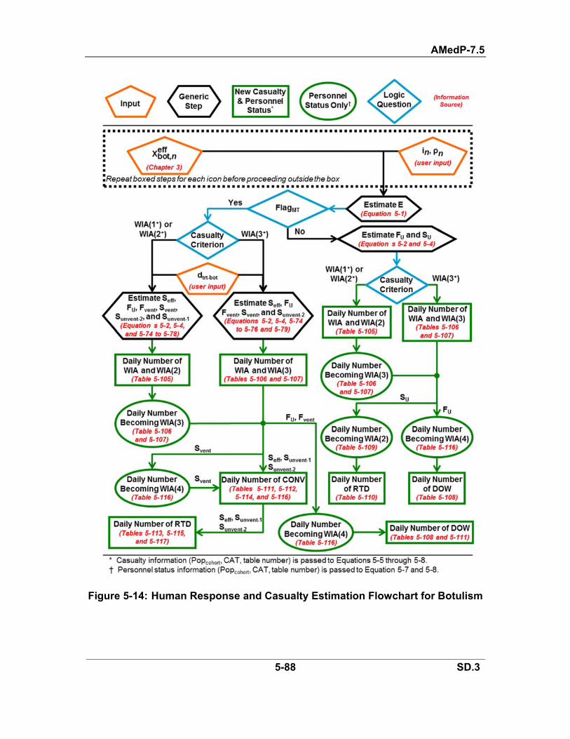
AMedP-7.5

5-88 SD.3

Figure 5-14: Human Response and Casualty Estimation Flowchart for Botulism

AMedP-7.5

5-89 SD.3

5.2.15. Ricin Intoxication

1. Figure 5-15 summarizes the human response and casualty estimation processes for ricin intoxication, Table 5-119 summarizes the Injury Profile, and Table 5-120 summarizes the other ricin intoxication submodels. No prophylaxis is modeled for ricin intoxication.

2. Assumptions.

a. All individuals are 70-kilogram males.

b. The effectivity probit slope is equal to the lethality probit slope.

3. Cohorts and special considerations.

a. Medical treatment has no effect on the submodel parameter values.

b. Because the duration of illness is dose-dependent, and that dose-dependence differs by stage of illness and by survivor versus non-survivor, the following steps must be taken.

1) The populations of E, F, and S are calculated using Equations 5-1, 5-2, and 5-4.

2) As Stage 1 and Stage 2 for survivors are both Severity Level 1, a separate table for the time at which survivors enter Stage 2 is not needed. Further, the time until Stage 1 and until RTD are fixed, so the dose-dependence of the length of Stage 1 has no practical bearing on the model. Thus, S is not split into sub-cohorts; it remains as S.

3) A different dose range is required for each stage of illness for non-survivors. As such, Table 5-118 lists the dose ranges for each stage of illness; the specific labels for the FDR cohorts differ by stage of illness.

Table 5-118: Ricin Intoxication Dose Ranges for the FDR Sub-Cohorts Duration of Stage 1 Duration of Stage 2 Duration of Stage 3

Dose Range Label (DR)

Dose Range (μg)

Dose Range Label (DR)

Dose Range (μg)

Dose Range Label (DR)

Dose Range (μg)

Stg2-A 0–<11 Stg3-A 0–<11 DOW-A 0–<13 Stg2-B 11–<41 Stg3-B 11–<24 DOW-B 13–<19 Stg2-C 41–<415 Stg3-C 24–<63 DOW-C 19–<30 Stg2-D ≥415 Stg3-D 63–<244 DOW-D 30–<50

Stg3-E 244–<2,455 DOW-E 50–<92 Stg3-F ≥2,455 DOW-F 92–<193 DOW-G 193–<504 DOW-H 504–<1,946 DOW-I 1,946–<19,619 DOW-J ≥19,619

4. Table 5-121 through Table 5-125 are the PDTs for ricin intoxication. The values

AMedP-7.5

5-90 SD.3

from a given table are to be used in Equations 5-5 through 5-8 with the cohort(s) listed in the table headers and footers, per Figure 5-15.

Table 5-119: Ricin Intoxication Injury Profile Stage Injury Severity Level

Non-Survivors (FDR) 1 1 2 3 3 4

Survivors (S) 1 1 2 1

Table 5-120: Ricin Intoxication Submodel Summary Type Value

Effectivity (pE Xricin,neff )

Lognormal Distribution Use Equation 5-32

ED50 = 120 μg Probit slope = 6.1 probits/log(dose)

Lethality (pf Xricin,neff )

Lognormal Distribution Use Equation 5-32

LD50 = 343 μg Probit slope = 6.1 probits/log(dose)

Latent Period*

Constant 6 hours Duration of Illness*

Stage 1: Non-Survivors (FDR)

Power Function Dose-dependent: <1–4 days

c = 6.1 r = -0.3

Stage 2: Non-Survivors (FDR)

Power Function Dose-dependent: <1–6 days

c = 4.3 r = -0.3

Stage 3: Non-Survivors (FDR)

Power Function Dose-dependent: <1–10 days

c = 9.0 r = -0.3

Stage 1: Survivors (S)

Power Function Dose-dependent: <1–6 days

c = 10.4 r = -0.3

Total Duration: Survivors (S) Constant 192 hours

* Presented for information only. These two submodels have already been convolved to generate the PDTs; the user should use the PDTs to estimate when changes in casualty category occur.

AMedP-7.5

5-91 SD.3

Table 5-121: Daily Fraction of Individuals Ill with Ricin Intoxication (E) Who Become WIA, for WIA(1+)

Day Fraction1 1.0000 ≥2 0.0000

* This equates to the time at which all cohorts enter Stage 1 (Severity Level 1). As Stage 2 for survivors is also Severity Level 1, a separate table indicating the time until Stage 2 is not needed.

Table 5-122: Dose-Dependent Day on Which Ricin Intoxication Non-Survivors (FStg2-X) Become WIA, for WIA(2+) or WIA(3+)

Day Dose Range Day Dose Range Day Dose Range ≥5 (none) 3 Stg2-B 1 Stg2-D 4 Stg2-A 2 Stg2-C

* This equates to the time at which all cohorts enter Stage 2 (Severity Level 3 for non-survivors and Severity Level 1 for survivors).

Table 5-123: Dose-Dependent Day on Which Ricin Intoxication Non-Survivors (FStg3-X) Enter Stage 3 of Illness

Day Dose Range Day Dose Range Day Dose Range ≥7 (none) 4 Stg3-C 1 Stg3-F 6 Stg3-A 3 Stg3-D 5 Stg3-B 2 Stg3-E

Table 5-124: Dose-Dependent Day on Which Ricin Intoxication Non-Survivors (FDR) DOW

Day Dose Range Day Dose Range Day Dose Range Day Dose Range≥11 (none) 8 DOW-C 5 DOW-F 2 DOW-I 10 DOW-A 7 DOW-D 4 DOW-G 1 DOW-J 9 DOW-B 6 DOW-E 3 DOW-H

Table 5-125: Daily Fraction of Ricin Intoxication Survivors (S) Who Become RTD

Day Fraction≤8 0.0000 9 1.0000 ≥10 0.0000

AMedP-7.5

5-92 SD.3

Figure 5-15: Human Response and Casualty Estimation Flowchart for Ricin Intoxication

5.2.16. Staphylococcal Enterotoxin B (SEB) Intoxication

1. Figure 5-16 summarizes the human response and casualty estimation processes for SEB intoxication, Table 5-127 summarizes the Injury Profile, and Table 5-128 summarizes the other SEB intoxication submodels. No prophylaxis is modeled for SEB intoxication.

2. Assumptions.

a. All individuals are 70-kilogram males.

b. The lethality probit slope is equal to the effectivity probit slope.

3. Cohorts and special considerations.

a. Medical treatment has no effect on the submodel parameter values.

b. The population of the E, F, and S cohorts are first calculated by applying

AMedP-7.5

5-93 SD.3

Equations 5-1, 5-2, and 5-4.

c. The S cohort is then split into sub-cohorts labeled as SDR, where DR is the dose range label given in Table 5-126. This is done due to the SEB intoxication Stage 1 duration of illness model for survivors being dose-dependent.

Table 5-126: SEB Intoxication Dose Ranges for the SDR Sub-Cohorts Dose Range Label (DR)

Dose Range (μg) Dose Range Label (DR)

Dose Range (μg)

XSEB,neff > XSEB,n

eff ≤ XSEB,neff > XSEB,n

eff ≤

A 0 0.0239 F 0.2824 0.3470 B 0.0239 0.0885 G 0.3470 0.4116 C 0.0885 0.1532 H 0.4116 0.4762 D 0.1532 0.2178 I 0.4762 E 0.2178 0.2824

4. Table 5-129 through Table 5-132 are the PDTs for SEB. The values from a given table are to be used in Equations 5-5 through 5-8 with the cohort(s) listed in the table headers and footers, per Figure 5-16.

Table 5-127: SEB Intoxication Injury Profile Stage Injury Severity Level

Non-Survivors (FDR) 1 3

Survivors (SDR) 1 3 2 1

Table 5-128: SEB Intoxication Submodel Summary Type Value

Effectivity (pE XSEB,neff )

Lognormal Distribution Use Equation 5-32

ED50 = 0.026 μg Probit slope = 2.44 probits/log(dose)

Lethality (pf XSEB,neff )

Lognormal Distribution Use Equation 5-32

LD50 = 1.4 μg Probit slope = 2.44 probits/log(dose)

Latent Period*

Constant 9 hours

Duration of Illness*

Stage 1: Survivors (SDR) Linear Function

(capped at 8 days) Dose-dependent: 1–8 days

m = 15.48 days/μg, b = 0.254 days Stage 2: Survivors (SDR)

Constant 7 days Stage 1: Non-Survivors (FDR)

Constant 3 days * Presented for information only. These two submodels have already been convolved to generate the

PDTs; the user should use the PDTs to estimate when changes in casualty category occur.

AMedP-7.5

5-94 SD.3

Table 5-129: Daily Fraction of Individuals Ill with SEB Intoxication (E) Who Become WIA, for Any Casualty Criterion

Day Fraction1 1.0000 ≥2 0.0000

* This equates to the time at which all cohorts enter Stage 1 (Severity Level 3).

Table 5-130: Daily Fraction of SEB Intoxication Non-Survivors (F) who DOW Day Fraction≤3 0.0000 4 1.0000 ≥5 0.0000

Table 5-131: Daily Fraction of SEB Intoxication Survivors (SDR) Who Enter Stage 2 of Illness

Day Dose Range Day Dose Range Day Dose Range Day Dose Range≤1 (none) 4 C 7 F 10 I 2 A 5 D 8 G ≥11 (none) 3 B 6 E 9 H

Table 5-132: Daily Fraction of SEB Intoxication Survivors (SDR) Who Become RTD

Day Dose Range Day Dose Range Day Dose Range Day Dose Range≤8 (none) 11 C 14 F 17 I 9 A 12 D 15 G ≥18 (none) 10 B 13 E 16 H

Figure 5-16: Human Response and Casualty Estimation Flowchart for SEB Intoxication

AMedP-7.5

5-95 SD.3

5.2.17. T-2 Mycotoxicosis

1. Figure 5-17 summarizes the human response and casualty estimation processes for T-2 mycotoxicosis, Table 5-133 summarizes the Injury Profile, and Table 5-134 summarizes the other T-2 mycotoxicosis submodels. No prophylaxis is modeled for T-2 mycotoxicosis.

2. Assumptions.

a. All individuals are 70-kilogram males.

b. The effectivity probit slope is equal to the lethality probit slope.

3. Cohorts and special considerations.

a. Medical treatment has no effect on the submodel parameter values.

b. The E, F, and S cohorts are used; their populations are calculated by applying Equations 5-1, 5-2, and 5-4.

4. Table 5-135 through Table 5-138 are the PDTs for T-2 mycotoxicosis. The values from a given table are to be used in Equations 5-5 through 5-8 with the cohort(s) listed in the table headers and footers, per Figure 5-17.

Table 5-133: T-2 Mycotoxicosis Injury Profile Stage Injury Severity Level

Non-Survivors (F)1 2 2 3 3 4

Survivors (S) 1 2 2 3

AMedP-7.5

5-96 SD.3

Table 5-134: T-2 Mycotoxicosis Submodel Summary Type Value

Effectivity (pE XT-2,neff )

Lognormal Distribution Use Equation 5-32

ED50 = 22.4 mg Probit slope = 4.3 probits/log(dose)

Lethality (pf XT-2,neff )

Lognormal Distribution Use Equation 5-32

LD50 = 28 mg Probit slope = 4.3 probits/log(dose))

Latent Period*

Constant 4 hours

Duration of Illness*

Stage 1: Non-Survivors (F) Stage 1: Survivors (S)

Constant 8 hours Stages 2 and 3 (each): Non-survivors (F)

Constant 4 hours Stage 2: Survivors (S)

Constant 14 days* Presented for information only. These two submodels have already been convolved to generate the

PDTs; the user should use the PDTs to estimate when changes in casualty category occur.

Table 5-135: Daily Fraction of Individuals Ill with T-2 Mycotoxicosis (E) Who Become WIA, for WIA(1+) or WIA(2+)*

Day Fraction1 1.0000 ≥2 0.0000

* This equates to the time at which all cohorts enter Stage 1 (Severity Level 2).

Table 5-136: Daily Fraction of Individuals Ill with T-2 Mycotoxicosis (E) Who Become WIA, for WIA(3+)*

Day Fraction1 1.0000 ≥2 0.0000

* This equates to the time at which all cohorts enter Stage 2 (Severity Level 3).

Table 5-137: Daily Fraction of T-2 Mycotoxicosis Non-Survivors (F) Who DOW*

Day Fraction1 1.0000 ≥2 0.0000

* This also equates to the time at which non-survivors enter Stage 3 (Severity Level 4).

Table 5-138: Daily Fraction of T-2 Mycotoxicosis Survivors (S) Who Become RTD

Day Fraction≤14 0.0000 15 1.0000 ≥16 0.0000

AMedP-7.5

5-97 SD.3

Figure 5-17: Human Response and Casualty Estimation Flowchart for T-2 Mycotoxicosis

5.2.18. Ebola Virus Disease

As noted in Section 1.3.1, this section presents some rough approximations of parameter values for EVD (Table 5-139).

Table 5-139: Approximate EVD Parameter Values Parameter Approximate Value or Range

Aerosol Infectivity Highly infectious; ID50 or threshold dose as low as < 10 PFU

Lethality Dependent on strain and quality of medical care Including all known outbreaks, CFR range is ~25 to ~90%

Incubation Period Mean: 5 to 13 days (strain dependent) Range: 2–21 days

Duration of Illness Non-survivors: mean 6 to 10 days Survivors: mean 14 to 19 days of acute illness, possibly followed by months of convalescence (post-Ebola syndrome)

INTENTIONALLY BLANK

AMedP-7.5

6-1 SD.3

CHAPTER 6 CASUALTY SUMMATION AND REPORTING

This chapter explains how the methodology’s outputs meet the requirements of AJP-4.10, and how the casualty estimate tables are generated from the outputs of Chapters 4 and 5. For specific guidance on how the outputs might be used, see AMedP-7.6. For additional operational, logistic, and medical planning considerations that may be affected by CBRN casualty estimates, see AJP-5, AJP-4, and AJP-4.10, respectively.

6.1. APPLICATION OF AJP-4.10 REQUIREMENTS

1. As stated in AJP-4.10, the casualty estimation process should generate four outputs: population at risk (PAR), casualty rates, casualty flow, and casualty profile.

2. In this methodology, the PAR is simply the total number of personnel included in the scenario, which is defined by user input and calculated according to 6-1. The user’s determination of which personnel should be included in a scenario should be guided by operational and medical considerations; AMedP-7.6 provides guidance on choosing the PAR.

PAR = inn

, (6-1)

where in is the number of individuals in icon n.

3. The casualty rate is concerned with the number of new casualties of each type per day. This methodology produces one table reporting the rate of new casualties, and an additional table, the personnel status table, that lists the total number of casualties reported in each category on each day.

4. The flow characterizes the movement between casualty categories.85 The casualty flow is depicted within the output tables; a separate table presenting the flow would be redundant.

5. The profile is a description of the relative proportions of types of injuries that relate to an individual’s casualty category. Profiles are presented within the output tables. Because different planning considerations are relevant for each casualty category, each category has a unique set of “compartments” that are used to describe the profile. See Table 6-1 for a summary of the compartments and the list below for explanation.

85 AJP-4.10 also describes flow as characterizing the timing of casualty waves. This is dependent on when incidents occur, which is beyond the purview of this methodology.

AMedP-7.5

6-2 SD.3

a. For KIA and DOW, the planning consideration is whether the human remains require special handling that would affect the operations of Mortuary Affairs. KIAs might be contaminated with chemical (C) or radiological materials (R or N), so the possible compartments are C, R, or N. DOWs might be biohazards (B) or might be uncontaminated86 (CRN).

b. For WIA and CONV, the planning consideration is the medical resources required to care for the casualty. Thus, for the rate table, WIAs are reported based on challenge type (e.g., WIA(GB) or WIA(anthrax)), and for the personnel status table, WIAs are reported based on both challenge type and injury severity (e.g., GB(4) or anthrax(2) within the WIA section of the table). CONV is reported only by the challenge (e.g., CONV(VX)).

c. RTD is not divided into compartments because, by definition, RTD personnel are capable of resuming normal duties.

Table 6-1: Compartments for Reporting Casualty Profile Casualty Category Basis for Compartment Names, or Specific Compartment Names

WIA Basis for names: challenge and Injury Severity Level KIA Specific names: chemical (C), radiological (R), or nuclear (N)

DOW Specific names: biological (B) or chemical/radiological/nuclear (CRN) CONV Basis for names: challenge RTD None

6.2. DESCRIPTION OF OUTPUT REPORTING

1. The casualty estimate is reported with a time resolution of one day. This time resolution is not user-tunable. Daily reporting continues until no more changes in casualty category occur.

2. As the rate table reports only new casualties, a casualty reported as WIA will not be reported again until s/he becomes DOW, CONV, or RTD. As the rate table cannot track subsequent changes in Injury Severity Level after an individual initially becomes WIA, they do not include the Injury Severity Level for WIAs.

3. The personnel status table gives the total number of casualties reported in each category on each day. As the personnel status table can track subsequent changes in Injury Severity Level, they report WIAs as WIA(#).

a. As casualties never leave the KIA, DOW, or RTD categories, the counts in the personnel status table are the cumulative number over time.

b. As casualties can leave the WIA and CONV categories, the counts in the personnel status table are the total on a given day, and over time the totals

86 Chemical and radiological casualties are assumed to be decontaminated prior to entering an MTF.

AMedP-7.5

6-3 SD.3

might peak and then decrease back to zero. When FlagMT = NO, the WIA totals might not decrease to zero (depending on the challenge type). Finally, for challenge types that produce permanent or indefinite CONV, CONV will not decrease to zero.

4. Because it is possible for an individual to be assigned to multiple casualty categories within a single day, the reporting rules from Table 1-4 are followed to facilitate more appropriate resource planning and to avoid double-counting. Adherence to these rules is built into the models described in Chapters 4 and 5.

5. Table 6-2 and Table 6-3 are example output tables. Note that for any particular incident, the tables may look different, per the following considerations.

a. The specific compartment labels are different for different challenge types (as specified in Table 6-1).

b. For brevity, rows that have 0 population on every day can be excluded.

1) In the personnel status table, WIA(#) rows can be excluded if the challenge type never causes injuries of that Injury Severity Level.

2) If there are no KIA, no DOW, no CONV, or no RTD, those rows can also be excluded.

c. A unique personnel status table is used for reporting nuclear casualties (see Section 6.3), to account for the simultaneous occurrence of radiation, blast, and thermal casualties, and the need to separately track different types of injury to facilitate medical planning.

Table 6-2: Estimated Daily Number of New (Challenge) Casualties* Casualty Description Day 1 Day 2 Day 3 Day 4 Day 5 Day 6 Day 7 Day 8 Day 9 Day Day X

New KIA (C, R, or N)

New DOW (CRN or B)

Sum of New Fatalities

New WIA (Challenge)

New CONV (Challenge)

New RTD * Estimate is based on Casualty Criterion WIA(X+), a PAR of Y, and FlagMT = Yes/No.

AMedP-7.5

6-4 SD.3

Table 6-3: Estimated Personnel Status for (Challenge) Casualties*

Casualty Description Day 1 Day 2 Day 3 Day 4 Day 5 Day 6 Day 7 Day 8 Day 9 Day Day X

Fatalities

KIA (C, R, or N)

DOW (CRN or B)

Sum of Fatalities

WIA

Challenge(1)

Challenge(2)

Challenge(3)

Challenge(4)

Sum of WIA

CONV

CONV (Challenge)

RTD

RTD * Estimate is based on Casualty Criterion WIA(X+), a PAR of Y, and FlagMT = Yes/No.

6. Chapters 4 and 5 provide the daily numbers of reported new casualties in each casualty category, to be entered in Table 6-2.

a. For chemical casualties, Equation 4-17 provides the daily numbers.

b. For radiological and nuclear casualties, Equation 4-18 provides the daily numbers.

c. For non-contagious biological casualties, Equations 5-5 and 5-6 provide the daily numbers.

d. For contagious biological casualties, Table 5-3 lists the equations to be used to provide the daily numbers.

7. Chapters 4 and 5 also provide the information needed to fill in the personnel status table, Table 6-3.

a. For chemical casualties, Equation 4-19 provides the daily numbers.

b. For radiological and nuclear casualties, Equation 4-20 provides the daily numbers.

c. For non-contagious biological casualties, Equations 5-7 and 5-8 provide the daily numbers.

d. For contagious biological casualties, Table 5-3 lists the equations to be used to provide the daily numbers.

8. A user interested in modeling multiple simultaneous incidents must run the

AMedP-7.5

6-5 SD.3

model separately for each incident and perform custom post-processing to combine the results.

a. If the incidents are all radiological or nuclear (for example, nuclear detonation and fallout), the icon-specific nature of the human response models will facilitate combining the results without any double-counting issues. Thus, generating casualty rate tables will be straightforward. However, a special version of the personnel status table should be used instead of Table 6-3—see Section 6.3.

b. If one of the multiple incidents is chemical or biological, double-counting some individuals and failing to account for other individuals will be unavoidable because of the population-based nature of the models.

6.3. PERSONNEL STATUS TABLE FOR NUCLEAR CASUALTIES

1. Although the methodology cannot account for synergy between radiation (R), blast (B), and thermal (T) challenges, it can produce a single report of casualties from the three prompt nuclear effects. The method is outlined here, and a specific example is given in Section A.6.

2. For each icon, the flowcharts for radiation (Figure 4-17), blast (Figure 4-18), and thermal (Figure 4-19) injury must be consulted, and the results combined. The following is guidance on how they are to be combined and how the output table is to be assembled.

a. If any of the three flowcharts indicates KIA, the icon should be reported as KIA on day 1.

b. Any icon that is WIA but not KIA should be reported as WIA on day 1, with the maximum severity of all three injuries on day 1 included. For example, (R2, B3, T2). Thus, the personnel status table will have up to 125 WIA rows (see Table 6-4). In most situations, many rows can be excluded from the table because their populations will be zero.

c. As indicated by the flowcharts, for days after day 1, an icon’s casualty status might be updated for one of several reasons.

1) Change in maximum severity of at least one of the three individual injuries—moves to a different WIA row. This can occur every day.

2) Casualty becomes DOW—moves from a WIA row to the DOW row. This occurs at the earliest time that any of the three flowcharts indicates.

3) Casualty becomes CONV—moves from a WIA row to a CONV row. This occurs at the latest time that any of the three flowcharts indicates.

AMedP-7.5

6-6 SD.3

4) Casualty becomes RTD—moves from a WIA row to the RTD row. This occurs at the latest time that any of the three flowcharts indicates.

4. Icons should only be reported as CONV for a single injury type if the medical treatment outcome reporting table indicates CONV. For example, if an icon receives R, B, and T injuries, and the B and T medical treatment outcome reporting tables indicate RTD, but the R table indicates CONV, that icon should be reported as CONV (R), not CONV (R, B, T).

5. Table 6-4 is an example personnel status table for nuclear casualties. It should be used instead of Table 6-3.

Table 6-4: Estimated Personnel Status for Nuclear Casualties*

Casualty Description Day 1 Day 2 Day 3 Day 4 Day 5 Day 6 Day 7 Day 8 Day 9 Day … Day X

Fatalities

KIA—N DOW—CRN

Sum of Fatalities

WIA†

R04.5–8.3 Gy, B0, T0§ R0, B0, T1

R0, B0, T2

R0, B0, T3

R0, B0, T4

R0, B1, T0

R0, B1, T1

R0, B1, T2

R0, B1, T3

R0, B1, T4

R0, B2, T0

R0, B2, T1

R0, B2, T2

R0, B2, T3

R0, B2, T4

R0, B3, T0

R0, B3, T1

R0, B3, T2

R0, B3, T3

R0, B3, T4

R0, B4, T0

R0, B4, T1

R0, B4, T2

R0, B4, T3

R0, B4, T4

R1, B0, T0

AMedP-7.5

6-7 SD.3

Casualty Description Day 1 Day 2 Day 3 Day 4 Day 5 Day 6 Day 7 Day 8 Day 9 Day … Day X

R1, B0, T1

R1, B0, T2

R1, B0, T3

R1, B0, T4

R1, B1, T0

R1, B1, T1

R1, B1, T2

R1, B1, T3

R1, B1, T4

R1, B2, T0

R1, B2, T1

R1, B2, T2

R1, B2, T3

R1, B2, T4

R1, B3, T0

R1, B3, T1

R1, B3, T2

R1, B3, T3

R1, B3, T4

R1, B4, T0

R1, B4, T1

R1, B4, T2

R1, B4, T3

R1, B4, T4

R2, B0, T0

R2, B0, T1

R2, B0, T2

R2, B0, T3

R2, B0, T4

R2, B1, T0

R2, B1, T1

R2, B1, T2

R2, B1, T3

R2, B1, T4

R2, B2, T0

R2, B2, T1

R2, B2, T2

R2, B2, T3

R2, B2, T4

R2, B3, T0

R2, B3, T1

R2, B3, T2

R2, B3, T3

AMedP-7.5

6-8 SD.3

Casualty Description Day 1 Day 2 Day 3 Day 4 Day 5 Day 6 Day 7 Day 8 Day 9 Day … Day X

R2, B3, T4

R2, B4, T0

R2, B4, T1

R2, B4, T2

R2, B4, T3

R2, B4, T4

R3, B0, T0

R3, B0, T1

R3, B0, T2

R3, B0, T3

R3, B0, T4

R3, B1, T0

R3, B1, T1

R3, B1, T2

R3, B1, T3

R3, B1, T4

R3, B2, T0

R3, B2, T1

R3, B2, T2

R3, B2, T3

R3, B2, T4

R3, B3, T0

R3, B3, T1

R3, B3, T2

R3, B3, T3

R3, B3, T4

R3, B4, T0

R3, B4, T1

R3, B4, T2

R3, B4, T3

R3, B4, T4

R4, B0, T0

R4, B0, T1

R4, B0, T2

R4, B0, T3

R4, B0, T4

R4, B1, T0

R4, B1, T1

R4, B1, T2

R4, B1, T3

R4, B1, T4

R4, B2, T0

R4, B2, T1

AMedP-7.5

6-9 SD.3

Casualty Description Day 1 Day 2 Day 3 Day 4 Day 5 Day 6 Day 7 Day 8 Day 9 Day … Day X

R4, B2, T2

R4, B2, T3

R4, B2, T4

R4, B3, T0

R4, B3, T1

R4, B3, T2

R4, B3, T3

R4, B3, T4

R4, B4, T0

R4, B4, T1

R4, B4, T2

R4, B4, T3

R4, B4, T4

Sum of WIA

CONV†

CONV (R) CONV (B)

CONV (T)

CONV (R, B)

CONV (R, T)

CONV (B, T)

CONV (R, B, T)

Sum of CONV

RTD

RTD * Estimate is based on Casualty Criterion WIA(X+) and a PAR of Y. † Any row that has a population of zero should be excluded from the table. § This row is for untreated individuals in the 4.5 – 8.3 Gy whole-body radiation dose range who either

sustained no thermal or blast injury, or have recovered from thermal or blast injuries; for the period between 72 and 96 hours, the radiation Injury Severity Level will be 0, but the Injury Severity Level will increase again at 96 hours, so the individuals cannot be RTD.

AMedP-7.5

6-10 SD.3

INTENTIONALLY BLANK

ANNEX A TO AMedP-7.5

A-1 SD.3

ANNEX A ILLUSTRATIVE EXAMPLES

A.1. OVERVIEW

1. This annex provides a set of six examples designed to act as a guide for the application of the methodology. Included are two chemical agents examples (GB and CK), one radiological example (a 137Cs RDD)87, a nuclear effects example (10 kT ground burst), and two biological agent examples (one non-contagious (anthrax) and one contagious (smallpox)).

2. For simplicity, the examples use a common force layout, described in Section A.2., which fulfills part of the INPUT step: it defines the icons and most of the icon attributes.

3. Next are the six illustrative examples (Sections A.3 through A.8), which each define a unique CBRN incident, and then walk through the remainder of the INPUT step and the CHALLENGE, RESPONSE, STATUS, and REPORT steps. The discussion of the five major steps for each example also includes finer detail on the methodological steps.

A.2. INPUT (ALL ILLUSTRATIVE EXAMPLES)

1. The illustrative examples will use Input Scheme 1 (see Figure 1-3).

2. Table 1-5 shows that for every agent, effect, or disease, Chapter 2 describes how to complete the INPUT step of the methodology. All INPUT other than the CBRN Challenge per icon over time is provided in this section (A.2); the CBRN Challenge information will be provided individually for each scenario (in Sections A.3 through A.8).

3. The following steps are necessary before the input described in Chapter 2 can be provided:

a. Define the layout of forces, grouping of individuals into icons, and values of icon attributes over time. This is done in Section A.2.1, specifically Table A-1.

b. Define a CBRN threat and model the CBRN incident. For the illustrative examples, this modeling has been done using specific U.S. software; in general, however, any national software or method that provides suitable output (Section 2.1.2 defines what is suitable) can be used. As mentioned, this step is different for each scenario, and will be discussed in Sections A.3

87 Methodologically, fallout and RDDs are almost identical, so a fallout example is unnecessary.

ANNEX A TO AMedP-7.5

A-2 SD.3

through A.8

A.2.1. Icons and Icon Attributes

1. The layout of forces is pictured in Figure A-1 and described in greater detail in Table A-1. The 816 personnel in the scenario are represented by 155 icons; it is an entirely notional force arranged as if guarding an airstrip (represented by the white space in the middle of the icons). A variety of vehicles and structures are listed in Table A-1 for the purpose of demonstrating the allowable variability among icons in a single scenario. The illustrative scenario is not meant to represent any real operation. The group of individuals represented by the icons will be referred to as the “task force”.

Figure A-1: Layout of Icons

2. Each of the 155 icons is assigned icon attributes per Table A-1. For the sake of simplicity, in five of the six illustrative examples these values will not change over time. However, to demonstrate how to handle changing icon attributes, the anthrax example will involve personnel initially not wearing IPE (masks), but then donning masks partway through the scenario (affects the CHALLENGE step).

3. The only other icon-specific information needed is the CBRN Challenge per icon over time, the values of which are provided Sections A.3 to A.8. The specific U.S. tools that were used to generate the CBRN Challenge per icon over time for the scenarios are listed below. These tools may not be available to other nations, and are

ANNEX A TO AMedP-7.5

A-3 SD.3

not required to execute AMedP-7.5; each nation should use its own national method of estimating CBRN challenge.

a. For all examples other than nuclear, the data were extracted from the results of simulations performed by the U.S. government software “Hazard Prediction and Assessment Capability” (HPAC), version 5.3.226 with Patch 3.88 Each icon was represented by an HPAC sampler; the type of sampler was specified so that data extracted from HPAC could be converted to the appropriate units for AMedP-7.5.

b. For the nuclear example, the radiation challenge was estimated according to Version 6 of Air Transport of Radiation (ATR6),89 and the thermal and blast challenges were estimated according to Calculational Tools Abstracted from DTRA’s Effects Manual One (EM-1).90

88 "Hazard Prediction and Assessment Capability," version 5.3.226 with Patch 3 (Defense Threat Reduction Agency, 2015). 89 F. Dolatshahi, D. C. Kaul, and W. A. Woolson, Technical and User’s Manual, Fortran Edition, Version 6 of Air Transport of Radiation (ATR6), SAIC-90/1507, DNA-TR-91-165 (La Jolla, CA: Science Applications International Corporation, 1992). 90 John A. Northrop, ed. Handbook of Nuclear Weapon Effects: Calculational Tools Abstracted from DTRA’s Effects Manual One (EM-1) (Ft. Belvoir, VA: Defense Threat Reduction Agency, 2002).

INTENTIONALLY BLANK

ANNEX A TO AMedP-7.5

A-4 SD.3

Table A-1: User Input for Illustrative Examples Tactical Scenario See Section: 2.1.3 2.1.4 2.1.5 2.1.6 2.1.6 4.4.4 4.4.4 4.4.4

Icon #

# Personnel

Activity Level

Body Surface

Area

IPE Class

Vehicle/Shelter Information

Ventilation Class Radiation

Class Thermal class

Icon Warned?

Uniform Type

1 4 Moderate 0.9 m2 None Shelter w/ColPro Tent Tent No BDU+T-shirt2 4 Moderate 0.9 m2 None Shelter w/ColPro Tent Tent No BDU+T-shirt

3 1 At Rest 0.9 m2 Mask Residential Building – Open

Windows Wood Frame

Building Wood Frame

Building No BDU+T-shirt

4 4 Moderate 0.9 m2 None Shelter w/ColPro Tent Tent No BDU+T-shirt

5 1 At Rest 0.9 m2 Mask Residential Building – Open

Windows Wood Frame

Building Wood Frame

Building No BDU+T-shirt

6 7 Moderate 0.9 m2 Mask None Foxhole Foxhole No BDU+T-shirt7 7 Moderate 0.9 m2 Mask None Foxhole Foxhole No BDU+T-shirt

8 7 Moderate 0.9 m2 Mask None Exposed/

Dismounted Exposed/

Dismounted No BDU+T-shirt

9 7 Moderate 0.9 m2 Mask None Exposed/

Dismounted Exposed/

Dismounted No BDU+T-shirt

10 7 Moderate 0.9 m2 Mask None Exposed/

Dismounted Exposed/

Dismounted No BDU+T-shirt

11 7 Moderate 0.9 m2 Mask None Foxhole Foxhole No BDU+T-shirt12 7 Moderate 0.9 m2 Mask None Foxhole Foxhole No BDU+T-shirt

13 7 Moderate 0.9 m2 Mask None Exposed/

Dismounted Exposed/

Dismounted No BDU+T-shirt

14 7 Moderate 0.9 m2 Mask None Foxhole Foxhole No BDU+T-shirt15 7 Moderate 0.9 m2 Mask None Foxhole Foxhole No BDU+T-shirt16 7 Moderate 0.9 m2 Mask None Foxhole Foxhole No BDU+T-shirt

17 7 Moderate 0.9 m2 Mask None Exposed/

Dismounted Exposed/

Dismounted No BDU+T-shirt

18 7 Moderate 0.9 m2 Mask None Foxhole Foxhole No BDU+T-shirt

19 7 Moderate 0.9 m2 Mask None Exposed/

Dismounted Exposed/

Dismounted No BDU+T-shirt

20 7 Moderate 0.9 m2 Mask None Foxhole Foxhole No BDU+T-shirt

ANNEX A TO AMedP-7.5

A-5 SD.3

See Section: 2.1.3 2.1.4 2.1.5 2.1.6 2.1.6 4.4.4 4.4.4 4.4.4

Icon #

# Personnel

Activity Level

Body Surface

Area

IPE Class

Vehicle/Shelter Information

Ventilation Class Radiation

Class Thermal class

Icon Warned?

Uniform Type

21 7 Moderate 0.9 m2 Mask None Exposed/

Dismounted Exposed/

Dismounted No BDU+T-shirt

22 7 Moderate 0.9 m2 Mask None Exposed/

Dismounted Exposed/

Dismounted No BDU+T-shirt

23 7 Moderate 0.9 m2 Mask None Exposed/

Dismounted Exposed/

Dismounted No BDU+T-shirt

24 7 Moderate 0.9 m2 Mask None Foxhole Foxhole No BDU+T-shirt25 7 Moderate 0.9 m2 Mask None Foxhole Foxhole No BDU+T-shirt

26 7 Moderate 0.9 m2 Mask None Exposed/

Dismounted Exposed/

Dismounted No BDU+T-shirt

27 7 Moderate 0.9 m2 Mask None Exposed/

Dismounted Exposed/

Dismounted No BDU+T-shirt

28 7 Moderate 0.9 m2 Mask None Foxhole Foxhole No BDU+T-shirt29 7 Moderate 0.9 m2 Mask None Foxhole Foxhole No BDU+T-shirt

30 7 Moderate 0.9 m2 Mask None Exposed/

Dismounted Exposed/

Dismounted No BDU+T-shirt

31 7 Moderate 0.9 m2 Mask None Exposed/

Dismounted Exposed/

Dismounted No BDU+T-shirt

32 7 Moderate 0.9 m2 Mask None Foxhole Foxhole No BDU+T-shirt

33 7 Moderate 0.9 m2 Mask None Exposed/

Dismounted Exposed/

Dismounted No BDU+T-shirt

34 7 Moderate 0.9 m2 Mask None Foxhole Foxhole No BDU+T-shirt

35 7 Moderate 0.9 m2 Mask None Exposed/

Dismounted Exposed/

Dismounted No BDU+T-shirt

36 7 Moderate 0.9 m2 Mask None Exposed/

Dismounted Exposed/

Dismounted No BDU+T-shirt

37 7 Moderate 0.9 m2 Mask None Foxhole Foxhole No BDU+T-shirt38 7 Moderate 0.9 m2 Mask None Foxhole Foxhole No BDU+T-shirt39 7 Moderate 0.9 m2 Mask None Foxhole Foxhole No BDU+T-shirt

40 7 Moderate 0.9 m2 Mask None Exposed/

Dismounted Exposed/

Dismounted No BDU+T-shirt

ANNEX A TO AMedP-7.5

A-6 SD.3

See Section: 2.1.3 2.1.4 2.1.5 2.1.6 2.1.6 4.4.4 4.4.4 4.4.4

Icon #

# Personnel

Activity Level

Body Surface

Area

IPE Class

Vehicle/Shelter Information

Ventilation Class Radiation

Class Thermal class

Icon Warned?

Uniform Type

41 7 Moderate 0.9 m2 Mask None Foxhole Foxhole No BDU+T-shirt

42 7 Moderate 0.9 m2 Mask None Exposed/

Dismounted Exposed/

Dismounted No BDU+T-shirt

43 7 Moderate 0.9 m2 Mask None Foxhole Foxhole No BDU+T-shirt

44 7 Moderate 0.9 m2 Mask None Exposed/

Dismounted Exposed/

DismountedNo BDU+T-shirt

45 7 Moderate 0.9 m2 Mask None Foxhole Foxhole No BDU+T-shirt46 7 Moderate 0.9 m2 Mask None Foxhole Foxhole No BDU+T-shirt47 7 Moderate 0.9 m2 Mask None Foxhole Foxhole No BDU+T-shirt

48 7 Moderate 0.9 m2 Mask None Exposed/

Dismounted Exposed/

Dismounted No BDU+T-shirt

49 7 Moderate 0.9 m2 Mask None Foxhole Foxhole No BDU+T-shirt

50 7 Moderate 0.9 m2 Mask None Exposed/

Dismounted Exposed/

Dismounted No BDU+T-shirt

51 7 Moderate 0.9 m2 Mask None Foxhole Foxhole No BDU+T-shirt52 7 Moderate 0.9 m2 Mask None Foxhole Foxhole No BDU+T-shirt

53 7 Moderate 0.9 m2 Mask None Exposed/

Dismounted Exposed/

Dismounted No BDU+T-shirt

54 7 Moderate 0.9 m2 Mask None Exposed/

Dismounted Exposed/

Dismounted No BDU+T-shirt

55 7 Moderate 0.9 m2 Mask None Exposed/

Dismounted Exposed/

Dismounted No BDU+T-shirt

56 7 Heavy 0.9 m2 Mask None Exposed/

Dismounted Exposed/

Dismounted No BDU+T-shirt

57 7 Heavy 0.9 m2 Mask None Exposed/

Dismounted Exposed/

Dismounted No BDU+T-shirt

58 7 Moderate 0.9 m2 Mask None Foxhole Foxhole No BDU+T-shirt

59 7 Heavy 0.9 m2 Mask None Exposed/

Dismounted Exposed/

Dismounted No BDU+T-shirt

60 7 Moderate 0.9 m2 Mask None Foxhole Foxhole No BDU+T-shirt

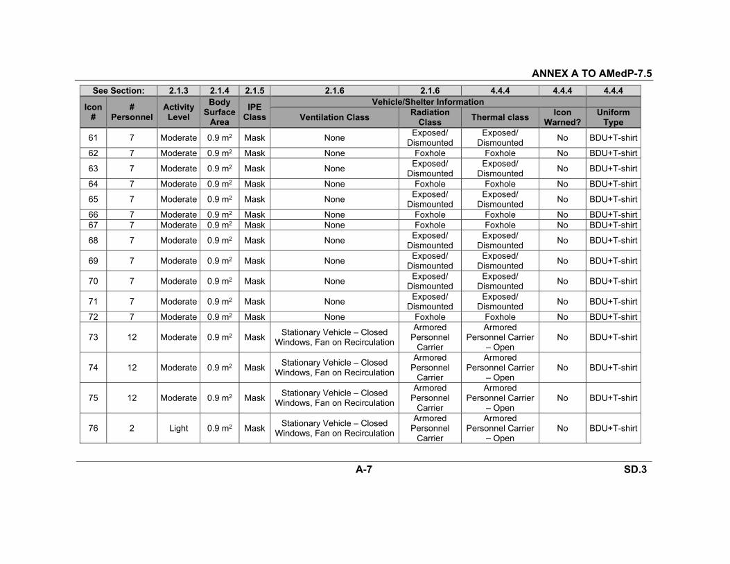
ANNEX A TO AMedP-7.5

A-7 SD.3

See Section: 2.1.3 2.1.4 2.1.5 2.1.6 2.1.6 4.4.4 4.4.4 4.4.4

Icon #

# Personnel

Activity Level

Body Surface

Area

IPE Class

Vehicle/Shelter Information

Ventilation Class Radiation

Class Thermal class

Icon Warned?

Uniform Type

61 7 Moderate 0.9 m2 Mask None Exposed/

Dismounted Exposed/

Dismounted No BDU+T-shirt

62 7 Moderate 0.9 m2 Mask None Foxhole Foxhole No BDU+T-shirt

63 7 Moderate 0.9 m2 Mask None Exposed/

Dismounted Exposed/

Dismounted No BDU+T-shirt

64 7 Moderate 0.9 m2 Mask None Foxhole Foxhole No BDU+T-shirt

65 7 Moderate 0.9 m2 Mask None Exposed/

Dismounted Exposed/

Dismounted No BDU+T-shirt

66 7 Moderate 0.9 m2 Mask None Foxhole Foxhole No BDU+T-shirt67 7 Moderate 0.9 m2 Mask None Foxhole Foxhole No BDU+T-shirt

68 7 Moderate 0.9 m2 Mask None Exposed/

Dismounted Exposed/

Dismounted No BDU+T-shirt

69 7 Moderate 0.9 m2 Mask None Exposed/

Dismounted Exposed/

Dismounted No BDU+T-shirt

70 7 Moderate 0.9 m2 Mask None Exposed/

Dismounted Exposed/

Dismounted No BDU+T-shirt

71 7 Moderate 0.9 m2 Mask None Exposed/

Dismounted Exposed/

Dismounted No BDU+T-shirt

72 7 Moderate 0.9 m2 Mask None Foxhole Foxhole No BDU+T-shirt

73 12 Moderate 0.9 m2 Mask Stationary Vehicle – Closed

Windows, Fan on Recirculation

Armored Personnel

Carrier

Armored Personnel Carrier

– Open No BDU+T-shirt

74 12 Moderate 0.9 m2 Mask Stationary Vehicle – Closed

Windows, Fan on Recirculation

Armored Personnel

Carrier

Armored Personnel Carrier

– Open No BDU+T-shirt

75 12 Moderate 0.9 m2 Mask Stationary Vehicle – Closed

Windows, Fan on Recirculation

Armored Personnel

Carrier

Armored Personnel Carrier

– Open No BDU+T-shirt

76 2 Light 0.9 m2 Mask Stationary Vehicle – Closed

Windows, Fan on Recirculation

Armored Personnel

Carrier

Armored Personnel Carrier

– Open No BDU+T-shirt

ANNEX A TO AMedP-7.5

A-8 SD.3

See Section: 2.1.3 2.1.4 2.1.5 2.1.6 2.1.6 4.4.4 4.4.4 4.4.4

Icon #

# Personnel

Activity Level

Body Surface

Area

IPE Class

Vehicle/Shelter Information

Ventilation Class Radiation

Class Thermal class

Icon Warned?

Uniform Type

77 2 Light 0.9 m2 Mask Stationary Vehicle – Closed

Windows, Fan on Recirculation

Armored Personnel

Carrier

Armored Personnel Carrier

– Open No BDU+T-shirt

78 2 Light 0.9 m2 Mask Stationary Vehicle – Closed

Windows, Fan on Recirculation

Armored Personnel

Carrier

Armored Personnel Carrier

– Open No BDU+T-shirt

79 2 Light 0.9 m2 Mask Stationary Vehicle – Closed

Windows, Fan on Recirculation

Armored Personnel

Carrier

Armored Personnel Carrier

– Open No BDU+T-shirt

80 2 Light 0.9 m2 Mask Stationary Vehicle – Closed

Windows, Fan on Recirculation

Armored Personnel

Carrier

Armored Personnel Carrier

– OpenNo BDU+T-shirt

81 2 Light 0.9 m2 Mask Stationary Vehicle – Closed

Windows, Fan on Recirculation

Armored Personnel

Carrier

Armored Personnel Carrier

– Open No BDU+T-shirt

82 2 Light 0.9 m2 Mask Stationary Vehicle – Closed

Windows, Fan on Recirculation

Armored Personnel

Carrier

Armored Personnel Carrier

– Open No BDU+T-shirt

83 2 Light 0.9 m2 Mask Stationary Vehicle – Closed

Windows, Fan on Recirculation

Armored Personnel

Carrier

Armored Personnel Carrier

– Open No BDU+T-shirt

84 4 Heavy 0.9 m2 Mask Stationary Vehicle – Closed

Windows, Fan on Recirculation

Armored Personnel

Carrier

Armored Personnel Carrier

– OpenNo BDU+T-shirt

85 4 Heavy 0.9 m2 Mask Stationary Vehicle – Closed

Windows, Fan on Recirculation

Armored Personnel

Carrier

Armored Personnel Carrier

– Open No BDU+T-shirt

86 4 Heavy 0.9 m2 Mask Stationary Vehicle – Closed

Windows, Fan on Recirculation

Armored Personnel

Carrier

Armored Personnel Carrier

– Open No BDU+T-shirt

ANNEX A TO AMedP-7.5

A-9 SD.3

See Section: 2.1.3 2.1.4 2.1.5 2.1.6 2.1.6 4.4.4 4.4.4 4.4.4

Icon #

# Personnel

Activity Level

Body Surface

Area

IPE Class

Vehicle/Shelter Information

Ventilation Class Radiation

Class Thermal class

Icon Warned?

Uniform Type

87 4 Heavy 0.9 m2 Mask Stationary Vehicle – Closed

Windows, Fan on Recirculation

Armored Personnel

Carrier

Armored Personnel Carrier

– Open No BDU+T-shirt

88 4 Heavy 0.9 m2 Mask Stationary Vehicle – Closed

Windows, Fan on Recirculation

Armored Personnel

Carrier

Armored Personnel Carrier

– Open No BDU+T-shirt

89 4 Moderate 0.9 m2 None Vehicle w/ColPro Armored

Personnel Carrier

Armored Personnel Carrier

– Open No BDU+T-shirt

90 4 Heavy 0.9 m2 None Vehicle w/ColPro Armored

Personnel Carrier

Armored Personnel Carrier

– OpenNo BDU+T-shirt

91 4 Moderate 0.9 m2 None Vehicle w/ColPro Armored

Personnel Carrier

Armored Personnel Carrier

– Open No BDU+T-shirt

92 2 Moderate 0.9 m2 None Shelter w/ColPro Tent Tent No BDU+T-shirt

93 4 Moderate 0.9 m2 None Vehicle w/ColPro Armored

Personnel Carrier

Armored Personnel Carrier

– Open No BDU+T-shirt

94 10 Moderate 0.9 m2 Mask Stationary Vehicle – Closed

Windows, Fan on Recirculation

Armored Personnel

Carrier

Armored Personnel Carrier

– Open No BDU+T-shirt

95 2 Moderate 0.9 m2 None Shelter w/ColPro Tent Tent No BDU+T-shirt

96 10 Moderate 0.9 m2 Mask Stationary Vehicle – Closed

Windows, Fan on Recirculation

Armored Personnel

Carrier

Armored Personnel Carrier

– Open No BDU+T-shirt

97 2 Moderate 0.9 m2 None Shelter w/ColPro Tent Tent No BDU+T-shirt

98 10 Moderate 0.9 m2 Mask Stationary Vehicle – Closed

Windows, Fan on Recirculation

Armored Personnel

Carrier

Armored Personnel Carrier

– Open No BDU+T-shirt

ANNEX A TO AMedP-7.5

A-10 SD.3

See Section: 2.1.3 2.1.4 2.1.5 2.1.6 2.1.6 4.4.4 4.4.4 4.4.4

Icon #

# Personnel

Activity Level

Body Surface

Area

IPE Class

Vehicle/Shelter Information

Ventilation Class Radiation

Class Thermal class

Icon Warned?

Uniform Type

99 10 Moderate 0.9 m2 Mask Stationary Vehicle – Closed

Windows, Fan on Recirculation

Armored Personnel

Carrier

Armored Personnel Carrier

– Open No BDU+T-shirt

100 10 Moderate 0.9 m2 Mask Stationary Vehicle – Closed

Windows, Fan on Recirculation

Armored Personnel

Carrier

Armored Personnel Carrier

– Open No BDU+T-shirt

101 10 Moderate 0.9 m2 Mask Stationary Vehicle – Closed

Windows, Fan on Recirculation

Armored Personnel

Carrier

Armored Personnel Carrier

– Open No BDU+T-shirt

102 10 Heavy 0.9 m2 Mask Stationary Vehicle – Open Windows, No Ventilation

Tent Tent No BDU+T-shirt

103 10 Moderate 0.9 m2 Mask Stationary Vehicle – Closed

Windows, Fan on RecirculationVan Semi-Trailer Van No BDU+T-shirt

104 4 Moderate 0.9 m2 Mask Stationary Vehicle – Open Windows, No Ventilation

Van Panel Van No BDU+T-shirt

105 10 Moderate 0.9 m2 Mask Stationary Vehicle – Closed

Windows, Fan on RecirculationVan Semi-Trailer Van No BDU+T-shirt

106 4 Moderate 0.9 m2 Mask None Exposed/

Dismounted Exposed/

Dismounted No BDU+T-shirt

107 10 Moderate 0.9 m2 Mask Stationary Vehicle – Closed

Windows, Fan on Recirculation

Armored Personnel

Carrier

Armored Personnel Carrier

– Open No BDU+T-shirt

108 1 Moderate 0.9 m2 Mask Stationary Vehicle – Open Windows, No Ventilation

Tent Tent No BDU+T-shirt

109 10 Moderate 0.9 m2 Mask Stationary Vehicle – Closed

Windows, Fan on RecirculationVan Semi-Trailer Van No BDU+T-shirt

110 1 Moderate 0.9 m2 Mask None Exposed/

Dismounted Exposed/

Dismounted No BDU+T-shirt

111 10 Moderate 0.9 m2 Mask Stationary Vehicle – Closed

Windows, Fan on RecirculationVan Semi-Trailer Van No BDU+T-shirt

112 3 Moderate 0.9 m2 Mask None Foxhole Foxhole No BDU+T-shirt

ANNEX A TO AMedP-7.5

A-11 SD.3

See Section: 2.1.3 2.1.4 2.1.5 2.1.6 2.1.6 4.4.4 4.4.4 4.4.4

Icon #

# Personnel

Activity Level

Body Surface

Area

IPE Class

Vehicle/Shelter Information

Ventilation Class Radiation

Class Thermal class

Icon Warned?

Uniform Type

113 4 Moderate 0.9 m2 Mask Stationary Vehicle – Open Windows, No Ventilation

Tent Tent No BDU+T-shirt

114 4 Moderate 0.9 m2 Mask Stationary Vehicle – Open Windows, No Ventilation

Tent Tent No BDU+T-shirt

115 10 Moderate 0.9 m2 None Vehicle w/ColPro Tank Tank – Movement No BDU+T-shirt116 10 Moderate 0.9 m2 None Vehicle w/ColPro Tank Tank – Movement No BDU+T-shirt

117 1 Heavy 0.9 m2 Mask Residential Building – Open

Windows Wood Frame

Building Wood Frame

Building No BDU+T-shirt

118 1 Heavy 0.9 m2 Mask Residential Building – Open

Windows Wood Frame

Building Wood Frame

Building No BDU+T-shirt

119 1 Heavy 0.9 m2 Mask Residential Building – Open

Windows Wood Frame

Building Wood Frame

Building No BDU+T-shirt

120 1 Moderate 0.9 m2 Mask None Foxhole Foxhole No BDU+T-shirt121 1 Moderate 0.9 m2 Mask None Foxhole Foxhole No BDU+T-shirt

122 1 Moderate 0.9 m2 Mask None Exposed/

Dismounted Exposed/

Dismounted No BDU+T-shirt

123 1 Heavy 0.9 m2 Mask Residential Building – Open

Windows Wood Frame

Building Wood Frame

Building No BDU+T-shirt

124 1 At Rest 0.9 m2 Mask Residential Building – Open

Windows Wood Frame

Building Wood Frame

Building No BDU+T-shirt

125 1 Moderate 0.9 m2 None Shelter w/ColPro Multi-Story

Brick BuildingMulti-Story Brick

Building No BDU+T-shirt

126 3 Heavy 0.9 m2 Mask Stationary Vehicle – Open Windows, No Ventilation

Van Panel Van No BDU+T-shirt

127 4 Heavy 0.9 m2 Mask Stationary Vehicle – Open Windows, No Ventilation

Van Panel Van No BDU+T-shirt

128 4 Moderate 0.9 m2 None Shelter w/ColPro Tent Tent No BDU+T-shirt

129 4 Moderate 0.9 m2 Mask Stationary Vehicle – Open Windows, No Ventilation

Van Panel Van No BDU+T-shirt

130 4 Moderate 0.9 m2 Mask Stationary Vehicle – Open Windows, No Ventilation

Tent Tent No BDU+T-shirt

ANNEX A TO AMedP-7.5

A-12 SD.3

See Section: 2.1.3 2.1.4 2.1.5 2.1.6 2.1.6 4.4.4 4.4.4 4.4.4

Icon #

# Personnel

Activity Level

Body Surface

Area

IPE Class

Vehicle/Shelter Information

Ventilation Class Radiation

Class Thermal class

Icon Warned?

Uniform Type

131 2 Moderate 0.9 m2 None Shelter w/ColPro Masonry Building

Masonry Building – Many Windows

No BDU+T-shirt

132 1 Moderate 0.9 m2 None Shelter w/ColPro Masonry Building

Masonry Building – Many Windows

No BDU+T-shirt

133 1 Moderate 0.9 m2 None Shelter w/ColPro Masonry Building

Masonry Building – Many Windows

No BDU+T-shirt

134 1 At Rest 0.9 m2 Mask Residential Building – Open

Windows Wood Frame

Building Wood Frame

Building No BDU+T-shirt

135 2 Moderate 0.9 m2 None Shelter w/ColPro Tent Tent No BDU+T-shirt136 5 Moderate 0.9 m2 Mask None Foxhole Foxhole No BDU+T-shirt

137 1 Moderate 0.9 m2 Mask Stationary Vehicle – Open Windows, No Ventilation

Tent Tent No BDU+T-shirt

138 1 Moderate 0.9 m2 Mask Stationary Vehicle – Open Windows, No Ventilation

Tent Tent No BDU+T-shirt

139 3 Moderate 0.9 m2 Mask None Foxhole Foxhole No BDU+T-shirt

140 4 Moderate 0.9 m2 Mask None Exposed/

Dismounted Exposed/

Dismounted No BDU+T-shirt

141 1 Heavy 0.9 m2 Mask Residential Building – Open

Windows Wood Frame

Building Wood Frame

Building No BDU+T-shirt

142 1 Heavy 0.9 m2 Mask Residential Building – Open

Windows Wood Frame

Building Wood Frame

Building No BDU+T-shirt

143 1 Heavy 0.9 m2 Mask Residential Building – Open

Windows Wood Frame

Building Wood Frame

Building No BDU+T-shirt

144 1 Moderate 0.9 m2 Mask Stationary Vehicle – Open Windows, No Ventilation

Van Panel Van No BDU+T-shirt

145 1 At Rest 0.9 m2 Mask Residential Building – Open

Windows Wood Frame

Building Wood Frame

Building No BDU+T-shirt

146 1 At Rest 0.9 m2 Mask Residential Building – Open

Windows Wood Frame

Building Wood Frame

Building No BDU+T-shirt

147 1 Moderate 0.9 m2 None Shelter w/ColPro Multi-Story

Brick BuildingMulti-Story Brick

Building No BDU+T-shirt

ANNEX A TO AMedP-7.5

A-13 SD.3

See Section: 2.1.3 2.1.4 2.1.5 2.1.6 2.1.6 4.4.4 4.4.4 4.4.4

Icon #

# Personnel

Activity Level

Body Surface

Area

IPE Class

Vehicle/Shelter Information

Ventilation Class Radiation

Class Thermal class

Icon Warned?

Uniform Type

148 3 Heavy 0.9 m2 Mask Stationary Vehicle – Open Windows, No Ventilation

Van Panel Van No BDU+T-shirt

149 3 Moderate 0.9 m2 Mask None Foxhole Foxhole No BDU+T-shirt

150 1 Moderate 0.9 m2 Mask Stationary Vehicle – Open Windows, No Ventilation

Tent Tent No BDU+T-shirt

151 6 Moderate 0.9 m2 None Shelter w/ColPro Tent Tent No BDU+T-shirt

152 1 Moderate 0.9 m2 Mask Stationary Vehicle – Open Windows, No Ventilation

Van Panel Van No BDU+T-shirt

153 6 Moderate 0.9 m2 None Shelter w/ColPro Tent Tent No BDU+T-shirt

154 1 Moderate 0.9 m2 None Shelter w/ColPro Masonry Building

Masonry Building – Many Windows

No BDU+T-shirt

155 1 Moderate 0.9 m2 None Shelter w/ColPro Masonry Building

Masonry Building – Many Windows

No BDU+T-shirt

ANNEX A TO AMedP-7.5

A-14 SD.3

A.2.2. Methodology Parameters

The values of the methodology parameters for the different scenarios have been chosen with the goal of illustrating different features of the methodology, but also minimizing the length of Annex A. Thus, in most cases, the default parameter values from Table 2-14 are used.

Table A-2: Values of Methodology Parameters for Illustrative Examples

Parameter GB CK 137Cs RDD Nuclear: 10 kT Ground

Anthrax Smallpox

TMTF 30 minutes 30 minutes 30 minutes 30 minutes 30 minutes 30 minutesTdeath-CN-SL4 15 minutes 15 minutes 15 minutes 15 minutes N/A N/A

FlagMT No*

Yes, MTGB=FMT* Yes

MTCK = AT Yes

No G-CSF Yes

No G-CSF Yes Yes

Casualty Criterion

WIA(1+) WIA(2+) WIA(1+) WIA(1+) WIA(1+) WIA(1+)* WIA(3+)*

dtrt-Q or dvac-spox

N/A N/A N/A N/A 7 12

* Separate examples for both options will be illustrated.

A.3. CHEMICAL AGENT: GB

1. The following excerpt from Table 1-5 shows which sections of AMedP-7.5 explain how to complete the five major steps for a GB casualty estimate.

Agent, Effect, or Disease Five Steps

INPUT CHALLENGE RESPONSE/STATUS REPORT

GB Ch. 2 Ch. 3 Sections 4.2.3 and 4.1 Ch. 6

2. In order to more easily follow along with the example, it is recommended that the reader print and have available for reference the following figures and tables: Figure 1-1, Figure 1-3, the annotated version of Figure 4-4 located on the next page, Table 4-4 to Table 4-6, and Table A-1.

3. The red octagons containing a single letter in the annotated version of Figure 4-4 are user aids to help link the text later in the GB example to the various parts of the flowchart. Specifically, the red octagons are used to mark the beginning of the

text discussion related to the linked flowchart element. For example, the on the first line of Section A.3.2 indicates that the discussion of the calculation of the

Effective CBRN Challenge (XGB,ih,neff ) begins there; is linked to the calculation of

XGB,ih,neff because of its placement in the annotated version of Figure 4-4.

ANNEX A TO AMedP-7.5

A-15 SD.3

Figure 4-4 Annotated for Illustrative Example

4. As noted in Table A-2, the GB example will illustrate the process for a casualty criterion of WIA(1+) and both possible values of FlagMT. The INPUT and CHALLENGE portions of the example are the same regardless of the value of FlagMT, as is a portion of the RESPONSE/STATUS section. The remainder of the RESPONSE/STATUS section and the REPORT section are different for different values of FlagMT.

A.3.1. INPUT

1. The only INPUT needed that was not given in Section A.2 is the CBRN Challenge per icon over time. This step is not associated with a red octagon because

ANNEX A TO AMedP-7.5

A-16 SD.3

it occurs in the flowchart of Figure 1-3, which is “upstream” of Figure 4-4. Finally, as stated in Section 2.1.2, the CBRN Challenge must be generated independently of AMedP-7.5, using national tools.

2. The simulated attack comprised 240 122 mm chemical rockets, each containing 2.4 kg of GB, for a total attack payload of 576 kg GB. The aim point was approximately at the center of mass of the icons on the airfield, and all 240 rockets detonated within 125 meters of the target. The simulated attack occurred at 2000 hours on cultivated terrain. Meteorological conditions were no cloud cover, wind at an average speed of about 2 m/s from the southwest toward the northeast, and an average temperature of 20.7 °C. Figure A-2 is a qualitative depiction of the CBRN Challenge (cumulative) at the end of the simulation. Each filled red circle represents an icon in the task force, and the GB plume is depicted with colors indicating different amounts of CBRN Challenge (purple is low, red is high).

3. To generate the quantitative input needed for AMedP-7.5, the CBRN Challenge per icon was extracted from HPAC in one-minute intervals. The extracted data for 8 selected icons are shown in Table A-3. Only the first 7 minutes are shown because after that time, no changes in CBRN Challenge occur for the 8 icons.

Figure A-2: GB Attack on Task Force

ANNEX A TO AMedP-7.5

A-17 SD.3

Table A-3: GB CBRN Challenge Data for Selected Icons

Icon # (n) XGB,ih,n,tk [mg-min/m3] at Time tk (min)

1 2 3 4 5 6 7

3 370.833 510.300 510.583 510.583 510.583 510.583 510.583 4 0 0.004 1.397 3.854 4.118 4.126 4.127 22 0 0.241 1.319 1.564 1.575 1.576 1.576 54 0 0.120 2.157 3.088 3.158 3.162 3.162 58 0 0.001 1.828 8.065 9.097 9.141 9.142 99 173.250 502.333 510.583 510.633 510.633 510.633 510.633

124 146.555 146.642 146.642 146.642 146.642 146.642 146.642 133 954.583 956.867 956.883 956.883 956.883 956.883 956.883

A.3.2. CHALLENGE

1. As indicated in Figure 4-4, the calculation of XGB,ih,n

eff is done per Chapter 3.

2. Because the icon attributes do not change over time, the sum in Equation 3-1 needs only a single term; the sum does not need to be expanded into a term for each minute of challenge data. Thus, Equation 3-1 for any icon can be simplified to:

XGB,ih,neff =

(XGB,ih,n,7 - 0) · Zn

APFGB,ih,n (3-1)

3. The value of XGB,ih,n,7 is in the Minute 7 column of Table A-3.

4. The value of Zn is determined by matching the specified Activity Level in Table A-1 with the corresponding unitless factor from Table 2-3. For example, Table A-1 specifies Moderate activity for icon 3, and Table 2-3 says that Moderate activity corresponds to a unitless factor of 2, so Z3 = 2.

5. The value of the aggregate protection factor (APFGB,ih,n) is calculated according to Sections 2.1.5, 2.1.6, 2.1.7, and 2.1.9. The details depend on the vehicle or shelter the icon occupies.

a. The protection factors for IPE and prophylaxis are straightforward to determine. The scenario does not include prophylaxis, so PFproph,GB,ih,n is 1 for all icons. The protection factor from IPE is determined by matching the specified IPE Class in Table A-1 with a PF in Table 2-4. For example, Table A-1 specifies that icon 99 is wearing masks, and Table 2-4 says that a mask gives an inhalation protection factor of 1667, so PFIPE,ih,99 = 1667.

b. Vehicle or shelter protection factor (PFV-SH,ih,n).

1) If the icon’s vehicle or shelter ventilation class is “None,” PFV-SH,ih,n = 1, per Table 2-6.

ANNEX A TO AMedP-7.5

A-18 SD.3

2) If the icon’s vehicle or shelter ventilation class is “Vehicle w/ColPro,” or “Shelter w/ColPro,” PFV-SH,ih,n = 3000, per Table 2-6.

3) If the icon is in a vehicle or shelter that does not have ColPro, Equation 2-1 must be used to calculate PFV-SH,ih,n. As an example, take icon 99: the vehicle is “Stationary Vehicle – Closed Windows, Fan on Recirculation.” According to Table 2-5, AER99 is 20. Table A-3 shows that the CBRN Challenge increases between the end of minute 1 and the end of minute 4, so Duration99 is 3 minutes or 0.05 hr. Since the input data specified that icons remain in their shelter or vehicle, Occupancy99 is until the end of the scenario, which is ill-defined. Arbitrarily assigning the value to 12 minutes, or 0.2 hr, the calculation of PFV-SH,ih,n is below. Note that as Occupancy increases beyond Duration, the PFV-SH,ih,n decreases.

PFV-SH,ih/pv,n=20·0.05

20·0.05 + e(-20·0.2) - e20·(0.05-0.2) = 1.07 (2-1)

c. Finally, according to Equation 2-2, the APF for icon 99, for example, is:

APFGB,ih,99 = PFIPE,GB,ih,99 · PFV-SH,GB,ih,99 · PFproph,GB,ih,99 = 1667 · 1.07 · 1 = 1784

6. Following the pattern of paragraphs 2 through 4, the entries in Table A-4 can be populated. Then, XGB,ih,n

eff is calculated by the simplified form of Equation 3-1 given at the end of paragraph A.3.2.2.

a. Because the IPE, vehicles, and shelters listed in Table A-1 protect so effectively, the calculated XGB,ih,n

eff for each icon in Table A-4 (and the entire scenario) are so low that very few casualties will occur.

b. Thus, for the purpose of illustrating the methodology, the calculation of XGB,ih,neff

is repeated with APFGB,ih,n set to 1—the results are labeled “Unprotected

XGB,ih,neff ” in Table A-4.

Table A-4: Calculation of GB Effective CBRN Challenge for Selected Icons

Icon # (n)

XGB,ih,n,7 [mg-min/m3]

Zn [unitless]

APFGB,ih,n [unitless]

XGB,ih,neff

[mg-min/m3]

Unprotected XGB,ih,n

eff [mg-min/m3]

3 510.583 0.5 2501 0.1021 255.29 4 4.127 2 3000 0.0028 8.25 22 1.576 2 1667 0.0019 3.15 54 3.162 2 1667 0.0038 6.32 58 9.142 2 1667 0.0110 18.28 99 510.633 2 1721 0.5934 1021.27 124 146.642 0.5 2440 0.0301 73.32 133 956.883 2 3000 0.6379 1914

ANNEX A TO AMedP-7.5

A-19 SD.3

7. The “Unprotected XGB,ih,neff ” values will be used for the rest of the GB example to

illustrate the RESPONSE, STATUS, and REPORT portions of the methodology.

A.3.3. RESPONSE/STATUS

1. According to Figure 4-4, with XGB,ih,n

eff and in available for all icons, the next step is to calculate the population of the Injury Profile cohorts (PopIPs), using Equations 4-1, 4-2, and 4-4, and Table 4-4.

a. Taking icon 58 as an example, XGB,ih,58eff is 18.28 mg-min/m3. Applying Equation

4-1 for all four levels of effect (values of k) makes use of the toxicity parameters given in Table 4-4:

pGB,ih_mild,58 = Φ PSGB,ih_mild· log10

XGB,ih,58eff

ECt50,GB,ih_mild=Φ 4.5· log10

18.28

0.4 = 1.0

pGB,ih_moderate,58 = Φ 12· log10

18.28

1.2 = 1.0

pGB,ih_severe,58 = Φ 12· log10

18.28

25 = 0.0514

pGB,ih_very severe,58 = Φ 12· log10

18.28

33 = 0.0010

b. Recall that the values calculated above must now be used to determine which fraction of personnel has each value of k as their worst level of effect (to avoid double-counting). According to Equation 4-2:

pw,GB,ih_mild,58 = pGB,ih_mild,58 - pGB,ih_moderate,58 = 0

pw,GB,ih_moderate,58 = pGB,ih_moderate,58 - pGB,ih_severe,58 = 0.9486

pw,GB,ih_severe,58 = pGB,ih_severe,58 - pGB,ih_very severe,58 = 0.0504

pw,GB,ih_very severe,58 = pGB,ih_very severe,58 - 0 = 0.0010

c. One may note that methodology will estimate that, for example, 0.3528 individuals from cohort 58 enter the Severe Injury Profile cohort. Although this may seem odd when considered at an individual level, the models are intended for application at the population level—that is, rounding to whole numbers of individuals will be done at the end of the process.

d. Using Equation 4-4 requires input related to all icons in the scenario, and the equation is rather straightforward, so it will not be demonstrated here. The

ANNEX A TO AMedP-7.5

A-20 SD.3

results of using Equations 4-1 and 4-2 for all 155 icons, and then using Equation 4-4, are given in Table A-5.

Table A-5: Injury Profile Cohort Populations for GB Illustrative Example Injury Profile Cohort Population (from Equation 4-4)

Mild 17.73 Moderate 39.26 Severe 0.64

Very Severe 183.72

2. According to Figure 4-4, the next step is to answer the question “Does the cohort become WIA?” using Figure 1-1 and the Injury Profiles (Table 4-5).

a. The casualty criterion is WIA(1+), per Table A-2; all cohorts become WIA.

3. The text at the bottom of Figure 4-4 states that certain information is passed to Equations 4-17 and 4-19. Paragraphs 4 and 5 (and sub-parts), below, will first summarize in plain text the information passed to the equations. Then, following the convention listed at the bottom of Figure 4-4, the information passed to the equations will be listed in this format: [PopIP, CAT, fnew-CAT, fex-CAT, d].

4. Still following Figure 4-4, the next several steps depend upon the value of FlagMT. First, consider the case in which FlagMT = No.

a. “At t < TMTF, is the Injury Severity Level 4 for longer than Tdeath-CN-SL4?”

1) For the Very Severe cohort, yes. The Very Severe cohort is reported as

KIA on Day 1. [183.72, KIA, 1.0, 0, 1]

2) For the Mild, Moderate, and Severe cohorts, no, so the flowchart indicates

“Report as WIA and WIA(#).” All three cohorts are reported as WIA on Day 1. The Mild, Moderate, and Severe cohorts are also reported as WIA(1), WIA(2), and WIA(3), respectively, on Day 1.

[17.73, WIA or WIA(1), 1.0, 0, 1] ; [39.26, WIA or WIA(2), 1.0, 0, 1] ; [0.64, WIA or WIA(3), 1.0, 0, 1]

b. “At t < TMTF, is the Injury Severity Level 4 for longer than Tdeath-CN-SL4?”

ANNEX A TO AMedP-7.5

A-21 SD.3

1) No, for all three remaining cohorts.

c. “Does the Injury Severity Level change?” and “Is the Injury Severity Level 0?”

1) The Mild cohort changes to Injury Severity Level 0 on Day 1. The Mild

cohort has already been reported as WIA and WIA(1) on Day 1, so it now must be reported as RTD on Day 2.

[17.73, WIA(1), 0, 1.0, 2] ; [17.73, RTD, 1.0, 0, 2]

2) The Moderate cohort changes to Injury Severity Level 1 at 1920 minutes

(32 hours); the Moderate cohort shall be reported as WIA(1) on Day 2, and will then have no further status change.

[39.26, WIA(2), 0, 1.0, 2] ; [39.26, WIA(1), 1.0, 0, 2]

3) The Severe cohort changes to Injury Severity Level 2 at 1920 minutes (32

hours) and to Injury Severity Level 1 at 8640 minutes (144 hours); the Severe cohort shall be reported as WIA(2) on Day 2, then as WIA(1) on Day 7, and will then have no further status change.

[0.64, WIA(3), 0, 1.0, 2] ; [0.64, WIA(2), 1.0, 0, 2] ; [0.64, WIA(2), 0, 1.0, 7] ; [0.64, WIA(1), 1.0, 0, 7]

5. Now consider the case in which FlagMT = Yes and MTGB = FMT, that is, following a different path through Figure 4-4.

a. “Report as WIA and WIA(#).”

1) All four cohorts are reported as WIA on Day 1. The Mild, Moderate, Severe, and Very Severe cohorts are also reported as WIA(1), WIA(2), WIA(3), and WIA(4), respectively, on Day 1.

[17.73, WIA or WIA(1), 1.0, 0, 1] ; [39.26, WIA or WIA(2), 1.0, 0, 1] ; [0.64, WIA or WIA(3), 1, 0, 1]; [183.72, WIA or WIA(4), 1.0, 0, 1]

b. “Report outcomes per Table 4-6.”

1) Per Table 4-6, the Mild cohort will be CONV on Day 2 and RTD on Day 8. [17.73, WIA(1), 0, 1.0, 2] ; [17.73, CONV, 1.0, 0, 2] ; [17.73, CONV, 0, 1.0, 8] ; [17.73, RTD, 1.0, 0, 8]

2) Per Section 4.1.1.6, the Moderate cohort will remain as WIA(2) for Day 2.

ANNEX A TO AMedP-7.5

A-22 SD.3

Per Table 4-6, the Moderate cohort will be CONV on Day 3 and RTD on Day 15.

[39.26, WIA(2), 0, 1.0, 3] ; [39.26, CONV, 1.0, 0, 3] ; [39.26, CONV, 0, 1.0, 15] ; [39.26, RTD, 1.0, 0, 15]

3) Per Section 4.1.1.6, the Severe cohort will remain as WIA(3) for Days 2 through 4. Then, per Table 4-6, 33.3 or 33.4% of the Severe cohort will become CONV on each of Days 5, 6, and 7, and on Day 31, 100% of the Severe cohort will become RTD.

[0.64, WIA(3), 0, 0.333, 5] ; [0.64, CONV, 0.333, 0, 5] [0.64, WIA(3), 0, 0.333, 6] ; [0.64, CONV, 0.333, 0, 6] [0.64, WIA(3), 0, 0.334, 7] ; [0.64, CONV, 0.334, 0, 7] [0.64, CONV, 0, 1.0, 31] ; [0.64, RTD, 1.0, 0, 31]

4) Per Section 4.1.1.6, survivors Very Severe cohort will become WIA(3), while any who will not survive will remain WIA(4) until they DOW. As MTGB = FMT, the threshold XGB,ih,n

eff that would cause an individual to die despite medical treatment is 165 mg-min/m3. Of the 183.72 in the Very Severe cohort, 161 had XGB,ih,n

eff above the threshold, so they will be DOW on Day 2. The remainder, 22.72, will be WIA(3) beginning Day 2, and CONV on Day 15.

[183.72, WIA(4), 0, 1.0, 2] ; [22.72, WIA(3), 1.0, 0, 2] ; [161, DOW, 1.0, 0, 2] [22.72, WIA(3), 0, 1.0, 15] ; [22.72, CONV, 1.0, 0, 15]

A.3.4. REPORT

1. Section A.3.3 stated the information that would be reported to Equations 4-17 and 4-19. This section will show how that information is used to populate the output tables.

2. As an example of the use of Equation 4-17, consider the application to determine the number of new WIA on Day 1 for the case in which FlagMT = No, using the reporting information from Section A.3.3.4. All reporting information for category WIA and day 1 must be considered; the relevant reporting information is: [17.73, WIA or WIA(1), 1.0, 0, 1] ; [39.26, WIA or WIA(2), 1.0, 0, 1] ; [0.64, WIA or WIA(3), 1.0, 0, 1].

NewWIA 1 = 17.73 · 1.0 + 39.26 · 1.0 + 0.64 · 1.0 = 57.63 58 (4-17)

The rate table (Table A-6) reports 58 casualties as new WIA on Day 1.

3. As an example of the use of Equation 4-19, consider the application to determine the total number of WIA(1) on Day 2 for the case in which FlagMT = No, using the reporting information from Section A.3.3.4. Equation 4-19 requires that the value for the previous day be known: TotWIA(1) 1 = 17.73. Then, all reporting information for category WIA(1) and day 2 must be considered; the relevant reporting

ANNEX A TO AMedP-7.5

A-23 SD.3

information is: [17.73, WIA(1), 0, 1.0, 2] ; [39.26, WIA(1), 1.0, 0, 2]

TotWIA(1) 2 = 17.73 + 17.73 · 0 - 1.0 + 39.26 · 1.0 - 0 = 39.26 39 (4-19)

The personnel status table (Table A-7) reports 39 casualties as WIA(1) on Day 2.

4. To complete all entries in the reporting tables, Equations 4-17 and 4-19 must be applied for all casualty categories and all days until no further changes occur. As the logic involved in applying the equations has been demonstrated, and for brevity, the remainder of the calculations are not shown here.

5. Table A-6 and Table A-7 are the output tables for the case in which FlagMT = No. Note that the estimates stop at Day 7 because no further changes in casualty status occur after Day 7.

Table A-6: Estimated Daily Number of New GB Casualties*

Casualty Description Day 1 Day 2 Day 3 Day 4 Day 5 Day 6 Day 7

New KIA (C) 184 0 0 0 0 0 0

New DOW (CRN) 0 0 0 0 0 0 0

Sum of New Fatalities 184 0 0 0 0 0 0

New WIA (GB) 58 0 0 0 0 0 0

New RTD 0 18 0 0 0 0 0 * Estimate is based on Casualty Criterion WIA(1+), a PAR of 816, and FlagMT = No.

Table A-7: Estimated Personnel Status for GB Casualties*

Casualty Description Day 1 Day 2 Day 3 Day 4 Day 5 Day 6 Day 7

Fatalities

KIA (C) 184 184 184 184 184 184 184

DOW (CRN) 0 0 0 0 0 0 0

Sum of Fatalities 184 184 184 184 184 184 184

WIA

GB(1) 18 39 39 39 39 39 40

GB(2) 39 1 1 1 1 1 0

GB(3) 1 0 0 0 0 0 0

Sum of WIA 58 40 40 40 40 40 40

RTD

RTD 0 18 18 18 18 18 18 * Estimate is based on Casualty Criterion WIA(1+), a PAR of 816, and FlagMT = No.

6. Table A-8 and Table A-9 and are the output tables for the case in which FlagMT = No. Note that the estimates stop at Day 31 because no further changes in casualty status occur after Day 31. Also note that due to the peculiarities of rounding, the total number of individuals accounted for in Table A-9 varies between 242 and 241, depending upon the day. The planner may use either estimate as the difference is

ANNEX A TO AMedP-7.5

A-24 SD.3

only one casualty.

Table A-8: Estimated Daily Number of New GB Casualties*

Casualty Description Day 1 Day 2 Day 3Days4–6

Day 7 Day 8Day9–14

Day 15

Day 16–30

Day 31

Day32+

KIA (C) 0 0 0 0 0 0 0 0 0 0 0

DOW (CRN) 0 0 0 0 0 0 0 0 0 0 0

Sum of New Fatalities 0 0 0 0 0 0 0 0 0 0 0

New WIA (GB) 241 0 0 0 0 0 0 0 0 0 0

New CONV (GB) 0 18 39 0 0 0 0 184 0 0 0

New RTD 0 0 0 0 0 18 0 39 0 1 0 * Estimate is based on Casualty Criterion WIA(1+), a PAR of 816, FlagMT = Yes, and MTGB = FMT.

Table A-9: Estimated Personnel Status for GB Casualties*

Casualty Description Day 1 Day 2 Day 3 Days 4–6

Day 7 Days 8–14

Days 15–30

Days 31+

Fatalities

KIA (C) 0 0 0 0 0 0 0 0

DOW (CRN) 0 161 161 161 161 161 161 161

Sum of Fatalities 0 161 161 161 161 161 161 161

WIA

GB(1) 18 0 0 0 0 0 0 0

GB(2) 39 39 0 0 0 0 0 0

GB(3) 1 23 23 23 23 23 0 0

GB(4) 184 0 0 0 0 0 0 0

Sum of WIA 241 63 23 23 23 23 0 0

CONV

CONV (GB) 0 18 57 57 58 40 23 23

RTD

RTD 0 0 0 0 0 18 57 58 * Estimate is based on Casualty Criterion WIA(1+), a PAR of 816, FlagMT = Yes, and MTGB = FMT.

A.4. CHEMICAL AGENT: CK

1. The following excerpt from Table 1-5 shows which sections of AMedP-7.5 explain how to complete the five major steps for a CK casualty estimate.

Agent, Effect, or Disease Five Steps

INPUT CHALLENGE RESPONSE/STATUS REPORT

CK Ch. 2 Ch. 3 Sections 4.2.12 and 4.1 Ch. 6

2. In order to more easily follow along with the example, it is recommended that the reader print and have available for reference the following figures and tables: Figure 1-1, Figure 1-3, the annotated version of Figure 4-13 located on the next page, Table 4-40 to Table 4-44, and Table A-1.

ANNEX A TO AMedP-7.5

A-25 SD.3

Figure 4-13 Annotated for Illustrative Example

3. The red octagons containing a single letter in the annotated version of Figure 4-13 are user aids to help link the text later in the CK example to the various parts of the flowchart. Specifically, the red octagons are used to mark the beginning of the

ANNEX A TO AMedP-7.5

A-26 SD.3

text discussion related to the linked flowchart element. For example, the on the first line of Section A.4.2 indicates that the discussion of the calculation of the

Effective CBRN Challenge (XCK,ih,neff ) begins there; is linked to the calculation of

XCK,ih,neff because of its placement in the annotated version of Figure 4-13.

4. As noted in Table A-2, the CK example will illustrate the process for a casualty criterion of WIA(2+) and FlagMT = Yes. Further, as was demonstrated in the GB example, the available protective measured are so effective that if they are used, few if any casualties will occur. As the GB example already demonstrated how to determine protection factors, this example will use the “unprotected” case in which all personnel are treated as having no IPE and being outside of any assigned vehicle or shelter.

A.4.1. INPUT

1. The only INPUT needed that was not given in Section A.2 is the CBRN Challenge per icon over time. This step is not associated with a red octagon because it occurs in the flowchart of Figure 1-3, which is “upstream” of Figure 4-13. Finally, as stated in Section 2.1.2, the CBRN Challenge must be generated independently of AMedP-7.5, using national tools.

2. The simulated attack comprised 720 122 mm chemical rockets, each containing 2.4 kg of CK, for a total attack payload of 1728 kg CK. The aim point was approximately at the center of mass of the icons on the airfield, and all 720 rockets detonated within 125 meters of the target. The simulated attack occurred at 2000 hours on cultivated terrain. Meteorological conditions were no cloud cover, wind at an average speed of about 2 m/s from the southwest toward the northeast, and an average temperature of 20.7 °C. Figure A-3 is a qualitative depiction of the CBRN Challenge (cumulative) at the end of the simulation. Each filled red circle represents an icon in the task force, and the CK plume is depicted with colors indicating different amounts of CBRN Challenge (purple is low, red is high).

3. To generate the quantitative input needed for AMedP-7.5, the CBRN Challenge per icon was extracted from HPAC. For the concentration-time CBRN Challenge, the values were extracted at one-minute intervals. However, for the CBRN Challenge for concentration-based effects, the values were extracted at one-second intervals; this was necessary because the CBRN Challenge for concentration-based effects is an instantaneous value (per the definition—Section 1.4), and peaks in the instantaneous value are very short lived (on the order of seconds, not minutes).

ANNEX A TO AMedP-7.5

A-27 SD.3

Figure A-3: CK Attack on Task Force

A.4.2. CHALLENGE

1. As indicated in Figure 4-13, the calculation of XCK,ih,n

eff is done per Chapter 3.

2. Because the icon attributes do not change over time, the sum in Equation 3-1 needs only a single term; the sum does not need to be expanded into a term for each minute of challenge data. Thus, Equation 3-1 for any icon can be simplified to:

XCK,ih,neff =

(XCK,ih,n,30 - 0) · Zn

1, (3-1)

where:

Minute 30 is chosen (XCK,ih,n,30) because the CBRN Challenge has stopped accumulating by that point, and

the APF, in the denominator, is set to 1 to model the unprotected case.

3. Similarly, Equation 3-2 can be simplified to:

ANNEX A TO AMedP-7.5

A-28 SD.3

XQ,neff = MAX

XQ,n,tk

1, for 0 ≤ k ≤ 1800, (3-2)

where:

the maximum value of k is 1800 because at one-second time resolution, 1,800 time points are in 30 minutes.

4. Table A-10 shows the two Effective CBRN Challenges, calculated using the simplified forms of Equations 3-1 and 3-2 given above, for 8 selected icons. The Table A-10 values will be used to illustrate the RESPONSE, STATUS, and REPORT portions of the methodology.

Table A-10: CK Effective CBRN Challenge for Selected Icons Icon #

(n) XCK,ih,n

eff [mg-min/m3]

XCK,[ih],neff

[mg/m3]

3 840.33 2652 11 8.50 3.6 23 1062.50 549 48 1677.57 783 58 125.40 69

101 3531.00 1709 131 5470.33 14448 132 3307.83 6257

A.4.3. RESPONSE/STATUS

1. According to Figure 4-13, with XCK,ih,n

eff , XCK,[ih],neff , and in now available for all

icons, the next step is to calculate the population of the Injury Profile cohorts (PopIPs), using Equations 4-1 to 4-3, 4-5 to 4-7, and Table 4-40 and Table 4-42.

a. Taking icon 132 as an example, XCK,ih,neff is 3307.83 mg-min/m3. Applying

Equation 4-1 for all four levels of effect (values of k) makes use of the toxicity parameters given in Table 4-40:

pCK,ih_mild,132 = Φ 12· log10

3307.83

1200 = 1.0

pCK,ih_moderate,132 = Φ 12· log10

3307.83

2100 = 0.991

pCK,ih_severe,132 = Φ 12· log10

3307.83

2800 = 0.807

ANNEX A TO AMedP-7.5

A-29 SD.3

pCK,ih_very severe,132 = Φ 12· log10

3307.83

4700 = 0.034

b. Recall that the values calculated above must now be used to determine which fraction of personnel has each value of k as their worst level of effect (to avoid double-counting). According to Equation 4-2:

pw,CK,ih_mild,132 = pCK,ih_mild,132 - pCK,ih_moderate,132 = 0.009

pw,CK,ih_moderate,132 = pCK,ih_moderate,132 - pCK,ih_severe,132 = 0.184

pw,CK,ih_severe,132 = pCK,ih_severe,132 - pCK,ih_very severe,132 = 0.773

pw,CK,ih_very severe,132 = pCK,ih_very severe,132 - 0 = 0.034

c. For concentration-based effects, the calculation is simpler. Again taking icon 132 as an example, XCK,[ih],n

eff = 6257 mg/m3. Applying Equation 4-3 for both effect levels makes use of the concentration ranges in Table 4-42.

pw,CK,[ih]_1-20,132 = 1 if 1 ≤ 6257 < 200 otherwise

= 0

pw,CK,[ih]_>20,132 = 1 if 20 ≤ 62570 otherwise

= 1

d. Now Equations 4-5 to 4-7 must be used. They are intended to be used to sum over all icons. For brevity, an example of applying the equations to icon 132 (i.e., as if icon 132 was the entire PAR) alone is shown below.

1) Equation 4-5 determines the populations of the Composite Injury Profile cohorts. Using icon 132 alone:

PopIP,CK,ih_mild,CK,[ih]_1-20 = i132 · pw,CK,ih_mild,132 · pw,CK,[ih]_1-20,132 = 1 · 0.009 · 0 =0

PopIP,CK,ih_mild,CK,[ih]_>20 = 1 · 0.009 · 1 =0.009

PopIP,CK,ih_moderate,CK,[ih]_1-20 = 1 · 0.184 · 1 =0

PopIP,CK,ih_moderate,CK,[ih]_>20 = 1 · 0.184 · 1 =0.184

PopIP,CK,ih_severe,CK,[ih]_1-20 = 1 · 0.773 · 1 =0

PopIP,CK,ih_severe,CK,[ih]_>20 = 1 · 0.773 · 1 =0.773

PopIP,CK,ih_very severe,CK,[ih]_1-20 = 1 · 0.034 · 1 =0

ANNEX A TO AMedP-7.5

A-30 SD.3

PopIP,CK,ih_very severe,CK,[ih]_>20 = 1 · 0.034 · 1 =0.034

2) Equation 4-6 is used to calculate the populations of the (non-composite) Injury Profiles for concentration-time based effects. For icon 132 alone:

PopIP,CK,ih_mild = i132 · pw,CK,ih_mild,132 - pw,CK,ih_mild,132 · pw,CK,[ih]_1-20,132 + pw,CK,ih_mild,132 · pw,CK,[ih]_>20,132

= 1 · 0.009 - 0.009 · 0 + 0.009 · 1 = 0

PopIP,CK,ih_moderate = 1 · 0.184 - 0.184 · 0 + 0.184 · 1 = 0

PopIP,CK,ih_severe = 1 · 0.773 - 0.773 · 0 + 0.773 · 1 = 0

PopIP,CK,ih_very severe = 1 · 0.034 - 0.034 · 0 + 0.034 · 1 = 0

3) Equation 4-7 is used to calculate the populations of the (non-composite) Injury Profiles for concentration based effects. For icon 132 alone:

PopIP,CK,[ih]_1-20 = i132 · pw,CK,[ih]_1-20,132 -

pw,CK,[ih]_1-20,132 · pw,CK,ih_mild,132 +

pw,CK,[ih]_1-20,132 · pw,CK,ih_moderate,132 +

pw,CK,[ih]_1-20,132 · pw,CK,ih_severe,132 +pw,CK,[ih]_1-20,132 · pw,CK,ih_very severe,132

= 1 · 0 - 0 · 0.009 + 0 · 0.184 + 0 · 0.773 + 0 · 0.034 = 0

PopIP,CK,[ih]_>20 = 1 · 1 - 1 · 0.009 + 1 · 0.184 + 1 · 0.773 + 1 · 0.034 = 0

4) For icon 132 alone, the populations of all the non-composite Injury Profile cohorts are zero; however, such is not the case when all icons are included; see Table A-11.

e. Applying Equations 4-1 to 4-3 and 4-5 to 4-7 to all 155 icons, instead of just icon 132, gives the results shown in Table A-11. Although in this case—and likely for most scenarios involving chemical agents with concentration-based effects, such as CG and CK—several injury profiles have zero population, this will usually not be true for agents that have two (or more) challenge types that both use median toxicities and probit slopes to calculate probabilities of effect (e.g., VX, HD).

ANNEX A TO AMedP-7.5

A-31 SD.3

Table A-11: Injury Profile Cohort Populations for CK Illustrative Example Injury Profile Cohort Population (from Equation 4-4)

Mild 0 Moderate 0 Severe 0

Very Severe 0 1–20 mg/m3 54.00 >20 mg/m3 190.63

Mild & 1–20 mg/m3 0 Mild & >20 mg/m3 36.84

Moderate & 1–20 mg/m3 0 Moderate & >20 mg/m3 23.07 Severe & 1–20 mg/m3 0 Severe & >20 mg/m3 26.84

Very Severe & 1–20 mg/m3 0 Very Severe & >20 mg/m3 23.87

2. Composite Injury Profiles for the profiles that are associated with a non-zero population must now be generated. This is done according to the flowchart in Figure 4-1. Because the process is straightforward, especially if Table 4-41 and Table 4-43 are available for reference, the results are simply shown below.

Table A-12: Inhaled CK Composite Injury Profiles

Time Point (min)

Injury Profile Mild &

> 20 mg/m3 Moderate & > 20 mg/m3

Severe & > 20 mg/m3

Very Severe & > 20 mg/m3

1 2 2 3 4 2 1 2 3 4 10 1 1 2 4 15 1 1 2 4*

120 0 1 1 180 0 0 1 480 0 0 0

* According to the default value for Tdeath-CN-SL4, death would be modeled at this point.

3. According to Figure 4-13, the next step is to answer the question “Does the cohort become WIA?”, for each cohort, using Figure 1-1 and the Injury Profiles (Table 4-41, Table 4-43, and Table A-12).

a. The casualty criterion is WIA(2+), so only cohorts involving Moderate, Severe, Very Severe, or >20 mg/m3 will become WIA.

4. The text at the bottom of Figure 4-13 states that certain information is passed to Equations 4-17 and 4-19. The subparts of this paragraph will first summarize in plain text the information passed to the equations. Then, following the convention

ANNEX A TO AMedP-7.5

A-32 SD.3

listed at the bottom of Figure 4-13, the information passed to the equations will be listed in this format: [PopIP, CAT, fnew-CAT, fex-CAT, d].

a. “At t < TMTF, is the Injury Severity Level 4 for longer than Tdeath-CN-SL4?”

1) For the Very Severe & >20 mg/m3 cohort, yes. The Very Severe & >20

mg/m3 cohort is reported as KIA on Day 1. [23.87, KIA, 1.0, 0, 1]

2) For all other cohorts, no, so the flowchart indicates “Report as WIA and

WIA(#).” All other cohorts that satisfy the casualty criterion are reported as WIA on Day 1. Additionally, the >20 mg/m3 and Moderate & >20 mg/m3 cohorts are reported as WIA(2) on Day 1, and the Severe & >20 mg/m3 cohort is reported as WIA(3) on Day 1.

[190.63, WIA or WIA(2), 1.0, 0, 1] ; [23.07, WIA or WIA(2), 1.0, 0, 1] ; [26.84, WIA or WIA(3), 1.0, 0, 1]

b. The value of FlagMT is Yes, per Table A-2. Thus, the next step is to “Report

outcomes per Table 4-44.”

1) Unlike in the GB example, the availability of medical treatment does not save the lives of those in the Very Severe cohorts. This is because treatment for CK is only available at the MTF, whereas treatment for GB begins in the field with individual-issue antidotes. Thus, no change occurs for the Very Severe & >20 mg/m3 cohort.

2) Table 4-44 indicates that all other cohorts will RTD on Day 2. [190.63, WIA(2), 0, 1.0, 2] ; [190.63, RTD, 1.0, 0, 2] [23.07, WIA(2), 0, 1.0, 2] ; [23.07, RTD, 1.0, 0, 2] [26.84, WIA(3), 0, 1.0, 2] ; [26.84, RTD, 1.0, 0, 2]

A.4.4. REPORT

1. Section A.4.3 stated the information that would be reported to Equations 4-17 and 4-19. This section will show how that information is used to populate the output tables.

2. As an example of the use of Equation 4-17, consider the application to determine the number of new RTD on Day 2, using the reporting information from Section A.4.3.3. The relevant reporting information is:

ANNEX A TO AMedP-7.5

A-33 SD.3

[190.63, RTD, 1.0, 0, 2] ; [23.07, RTD, 1.0, 0, 2] ; [26.84, RTD, 1.0, 0, 2]

NewRTD 2 = 190.63 · 1.0 + 23.07 · 1.0 + 26.84 · 1.0 = 240.54 241 (4-17)

The rate table (Table A-13) reports 241 casualties as new RTD on Day 2.

3. As an example of the use of Equation 4-19, consider the application to determine the total number of WIA(2) on Day 2, using the reporting information from Section A.4.3.3. Equation 4-19 requires that the value for the previous day be known: TotWIA(2) 1 = 213.70. Then, all reporting information for category WIA(2) and day 2 must be considered; the relevant reporting information is: [190.63, WIA(2), 0, 1.0, 2] ; [23.07, WIA(2), 0, 1.0, 2]

TotWIA(2) 2 = 213.70 + 190.63 · 0 - 1.0 + 23.07 · 1.0 - 0 = 0 (4-19)

The personnel status table (Table A-14) reports 0 casualties as WIA(2) on Day 2.

4. To complete all entries in the reporting tables, Equations 4-17 and 4-19 must be applied for all casualty categories and all days until no further changes occur. As the logic involved in applying the equations has been demonstrated, and for brevity, the remainder of the calculations are not shown here.

5. Table A-13 and Table A-14 are the output tables for the CK example. Note that the estimates stop at Day 2 because no further changes in casualty status occur after Day 2.

Table A-13: Estimated Daily Number of New CK Casualties*

Casualty Description Day 1 Day 2

New KIA (C) 24 0

New DOW (CRN) 0 0

Sum of New Fatalities 24 0

New WIA (CK) 241 0

New CONV (CK) 0 0

New RTD 0 241 * Estimate is based on Casualty Criterion WIA(2+), a PAR of 816, FlagMT = Yes, and MTCK = AT.

ANNEX A TO AMedP-7.5

A-34 SD.3

Table A-14: Estimated Personnel Status for CK Casualties*

Casualty Description Day 1 Day 2

Fatalities

KIA (C) 24 24

DOW (CRN) 0 0

Sum of Fatalities 24 24

WIA

CK(2) 214 0

CK(3) 27 0

Sum of WIA 241 0

CONV

CONV (CK) 0 0

RTD

RTD 0 241 * Estimate is based on Casualty Criterion WIA(2+), a PAR of 816, FlagMT = Yes, and MTCK = AT.

A.5. RDD: 137CS

1. The following excerpt from Table 1-5 shows which sections of AMedP-7.5 explain how to complete the five major steps for a RDD casualty estimate.

Agent, Effect, or Disease Five Steps

INPUT CHALLENGE RESPONSE/STATUS REPORT

RDD Ch. 2 Ch. 3 and Section 4.3.2.3 Sections 4.3.2 and 4.1 Ch. 6

2. In order to more easily follow along with the example, it is recommended that the reader print and have available for reference the following figures and tables: Figure 1-1, Figure 1-3, the annotated version of Figure 4-15 located on the next page, Table 4-49 to Table 4-54, and Table A-1.

3. The red octagons containing a single letter in the annotated version of Figure 4-15 are user aids to help link the text later in the RDD example to the various parts of the flowchart. Specifically, the red octagons are used to mark the beginning of the

text discussion related to the linked flowchart element. For example, the and on the first line of Section A.5.2 indicate that the discussion of the calculation of the

Effective CBRN Challenges (XRDD,wb,neff XRDD,cut,n

eff ) begins there; is linked to the

calculation of XRDD,wb,neff and is linked to the calculation of XRDD,cut,n

eff because of their placement in the annotated version of Figure 4-15.

4. As noted in Table A-2, the RDD example will illustrate the process for a casualty criterion of WIA(1+), FlagMT = Yes, and without including the effects of G-CSF as part of medical treatment. The full protection indicated in Table A-1 is included.

ANNEX A TO AMedP-7.5

A-35 SD.3

Figure 4-15 Annotated for Illustrative Example

ANNEX A TO AMedP-7.5

A-36 SD.3

A.5.1. INPUT

1. The only INPUT needed that was not given in Section A.2 is the CBRN Challenge per icon over time. This step is not associated with a red octagon because it occurs in the flowchart of Figure 1-3, which is “upstream” of Figure 4-15. Finally, as stated in Section 2.1.2, the CBRN Challenge must be generated independently of AMedP-7.5, using national tools.

2. The simulated attack is a 1,000 kg high explosive91 that disperses 1.11×105 TBq of 137Cs (equivalent to the typical source strength of an irradiator used for sterilization and food preservation). The point of detonation is 1 m above ground and less than 200 m west of the westernmost extent of the task force. The simulated attack occurred at 2000 hours on cultivated terrain. Meteorological conditions were no cloud cover, wind at an average speed of about 2 m/s from the southwest toward the northeast, and an average temperature of 20.7 °C. Figure A-4 is a qualitative depiction of the CBRN Challenge (cumulative) at the end of the simulation. Each filled red circle represents an icon in the task force, and the 137Cs plume is depicted with colors indicating different amounts of CBRN Challenge (grey is low, yellow is high).

3. To generate the quantitative input needed for AMedP-7.5, the CBRN Challenge per icon was extracted from HPAC in one-minute intervals. As full protection is included for the entire challenge duration, only the final value of the CBRN Challenge—the value at 240 minutes—is needed for the calculations. Overall, very few icons received a challenge sufficient to cause casualties, and of those that did, only some of the dose ranges are represented. Thus, data for only 3 selected icons are shown in Table A-15.

91 Direct effects of the explosive—i.e. trauma—are not modeled; only the effects of the dispersed 137Cs are modeled.

ANNEX A TO AMedP-7.5

A-37 SD.3

Figure A-4: 137Cs RDD Attack on Task Force

Table A-15: RDD CBRN Challenge Data for Selected Icons Icon

# (n)

Contributors to XRDD,wb,neff [Gy] Contributors to XRDD,cut,n

eff [Gy] XRDD,wb,cld,n,240 [TBq-min/m3]

XRDD,wb,grd,n,240

[TBq-min/m2]XRDD,wb,ih,n,240

[TBq-min/m3]XRDD,cut,cld,n,240

[TBq-min/m3]XRDD,cut,grd,n,240 [TBq-min/m2]

XRDD,cut,s,n,240

[TBq-min/m3]1 0.00211 2.57255 0.00211 0.00211 2.57255 2.57255 26 0.00658 36.0650 0.00658 0.00658 36.0650 36.0650 36 0.00366 17.1343 0.00366 0.00366 17.1343 17.1343

A.5.2. CHALLENGE

1. Section 4.3.2, and in particular Equations 4-23 to 4-25 and 4-27 to 4-29 indicate the need to sum over different isotopes to determine the total cloudshine, groundshine, inhalation, or skin contamination effective dose. As this example uses a single isotope (137Cs), such summing is unnecessary. Equation 3-1 will be used six times: once each for cloudshine, groundshine, and inhalation for the whole-body challenge, and once each for cloudshine, groundshine, and skin contamination for the cutaneous challenge.

2. Because the icon attributes do not change over time, the sum in Equation 3-1 needs only a single term; the sum does not need to be expanded into a term for each minute of challenge data. Thus, Equation 3-1 for any icon can be simplified to:

ANNEX A TO AMedP-7.5

A-38 SD.3

XRDD,Q,neff =

(XRDD,Q,n,60 - 0) · Z

APFRDD,Q,n, (3-1)

where:

Minute 60 is chosen because all CBRN Challenges have stopped accumulating by that point,

Z will depend upon whether the challenge is cloudshine, groundshine, inhalation, or skin contamination (values are in Table 3-1),

The value of APFRDD,Q,n is calculated according to Sections 2.1.5, 2.1.6, 2.1.7., and 2.1.9. The details depend upon the vehicle or shelter the icon occupies.

3. The value of the APF is specific to the challenge.

a. For cloudshine and groundshine challenges (components of both whole-body and cutaneous), only a vehicle or shelter might provide protection. As 137Cs emits primarily gamma radiation, protection factors from the gamma column of Table 2-7 are used. Icon 1 is in a Tent, and icons 26 and 36 are Exposed/Dismounted, all of which give no protection (APF = 1).

b. For the inhalation challenge (a component of whole-body), the APF calculation is exactly the same as those demonstrated for the chemical agents—the process will not be demonstrated again here (see Sections A.3 and A.4 for details).

c. For the skin contamination challenge (a component of cutaneous), the only relevant protection factors are those on the right-most column of Table 2-4, and as none of the icons in this scenario are wearing Full Protection IPE, the APFs are 1.

4. Table A-16 shows the two Effective CBRN Challenges for each of the three selected icons. Icon 26 is the only icon with a whole-body dose sufficient to cause injury, and most other icons have cutaneous dose on the order or 10 Gy, such that they are in the same dose range as either Icon 1 or Icon 36.

Table A-16: RDD Effective CBRN Challenge for Selected Icons Icon #

(n) XRDD,wb,neff [Gy] XRDD,cut,n

eff [Gy]

1 0.10 4.4 26 1.28 61.9 36 0.61 29.4

ANNEX A TO AMedP-7.5

A-39 SD.3

A.5.3. RESPONSE/STATUS

1. According to Figure 4-15, the first step now that the Effective CBRN Challenges are known is to determine dose ranges.

a. Icon 1’s dose ranges are < 1.25 Gy (WB) and 2 –< 15 Gy (cut).

b. Icon 26’s dose ranges are 1.25 –< 3 Gy (WB) and 40 –< 550 Gy (cut)

c. Icon 36’s dose ranges are < 1.25 Gy (WB) and 15 –< 40 Gy (cut).

2. The next step is to generate Composite Injury Profiles, as needed. Icons 1 and 36 do not need Composite Injury Profiles because they will not suffer a whole-body injury. For Icon 26, the Composite Injury Profile is generated using the scheme in Figure 4-1 with Table 4-50 and Table 4-53. The Composite Injury Profile is shown in Table A-17.

Table A-17: Icon 26 Combined Injury Profile Time Point

(hr) 1.25 –< 3 Gy (WB) and 40 –< 550 Gy (cut)

0.1 0

1 1

8 1

10 1

24 1

48 2

192 3

3. Table A-18 shows the number of individuals that belong to each possible dose range combination, across the entire task force. Icon 26 has a population of 7 personnel, and is the only icon represented by the 1.25 – < 3 Gy and 40 – < 550 Gy row.

Table A-18: Dose Range Combination Distribution Across the Task Force Whole-Body Dose Range Cutaneous Dose Range Number of Individuals

< 1.25 Gy < 2 Gy 575*

1.25 – < 3 Gy < 2 Gy 0 ≥ 3 Gy < 2 Gy 0

< 1.25 Gy 2 – < 15 Gy 213 1.25 – < 3 Gy 2 – < 15 Gy 0

≥ 3 Gy 2 – < 15 Gy 0 < 1.25 Gy 15 – < 40 Gy 21

1.25 – < 3 Gy 15 – < 40 Gy 0 ≥ 3 Gy 15 – < 40 Gy 0

< 1.25 Gy 40 – < 550 Gy 0 1.25 – < 3 Gy 40 – < 550 Gy 7

≥ 3 Gy 40 – < 550 Gy 0

ANNEX A TO AMedP-7.5

A-40 SD.3

Whole-Body Dose Range Cutaneous Dose Range Number of Individuals

< 1.25 Gy ≥ 550 Gy 0 1.25 – < 3 Gy ≥ 550 Gy 0

≥ 3 Gy ≥ 550 Gy 0 * These individuals are not casualties.

4. For the next several steps, following the convention listed at the bottom of Figure 4-15, the information passed to the equations will be listed in this format: [in, CAT, fnew-CAT, fex-CAT, d].

5. The next step in Figure 4-15 is to determine whether the icons become WIA, and if so, report them as such. All three selected icons from Table A-16 become WIA(1) on Day 1.

[4, WIA or WIA(1), 1.0, 0, 1] ; [7, WIA or WIA(1), 1.0, 0, 1] [7, WIA or WIA(1), 1.0, 0, 1]

6. Because FlagMT = Yes, the next step is to report outcomes according to the medical treatment tables (Table 4-51 and/or Table 4-54).

a. For Icon 1, Table 4-51 indicates RTD on Day 3. [4, WIA(1), 0, 1.0, 3] ; [4, RTD, 1.0, 0, 3]

b. For Icon 26, Table 4-51 indicates CONV on Day 3, and Table 4-54 indicates CONV on Day 2. The later date takes precedence. [7, WIA(1), 0, 1.0, 3] ; [7, CONV, 1.0, 0, 3]

c. For Icon 36, Table 4-51 indicates RTD on Day 3. [7, WIA(1), 0, 1.0, 3] ; [7, RTD, 1.0, 0, 3]

A.5.4. REPORT

1. Section A.5.3 stated the information that would be reported to Equations 4-18 and 4-20. This section will show how that information is used to populate the output tables.

2. As an example of the use of Equation 4-18, consider the application to determine the number of new WIA on Day 1, using the reporting information from Section A.5.3. All reporting information for category WIA and day 1 must be considered; the relevant reporting information is: [4, WIA or WIA(1), 1.0, 0, 1] ; [7, WIA or WIA(1), 1.0, 0, 1] ; [7, WIA or WIA(1), 1.0, 0, 1].

NewWIA 1 = 4 · 1.0 + 7 · 1.0 + 7 · 1.0 = 18 (4-17)

The rate table (Table A-19) reports a larger number of casualties on Day 1

ANNEX A TO AMedP-7.5

A-41 SD.3

because it accounts for all icons.

3. As an example of the use of Equation 4-20, consider the application to determine the total number of WIA(1) on Day 3, using the reporting information from Section A.5.3. Equation 4-19 requires that the value for the previous day be known: for the three selected icons alone, TotWIA(1) 2 = 18. Then, all reporting information for category WIA(1) and Day 3 must be considered; the relevant reporting information is: [4, WIA(1), 0, 1.0, 3] ; [7, WIA(1), 0, 1.0, 2] ; [7, WIA(1), 0, 1.0, 2]

TotWIA(1) 3 = 18 + 4 · 0 - 1.0 + 7 · 0 - 1.0 + 7 · 0 - 1.0 = 0 (4-19)

The personnel status table (Table A-20) also reports zero casualties on day 3, even though it considers additional icons

4. To complete all entries in the reporting tables, Equations 4-18 and 4-20 must be applied for all casualty categories and all days until no further changes occur. As the logic involved in applying the equations has been demonstrated, and for brevity, the remainder of the calculations are not shown here.

5. Table A-19 and Table A-20 are the output tables. To demonstrate a different way of presenting results, “planning ranges” have been applied such that days 8–14 are combined, days 15–30 are combined, and days 31+ are combined. This is entirely flexible and user-specifiable.

Table A-19: Estimated Daily Number of New 137Cs RDD Casualties*

Casualty Description Day 1 Day 2 Day 3 Day 4 Day 5 Day 6 Day 7Days 8–14

Days 15–30

Days 31+

New KIA (R) 0 0 0 0 0 0 0 0 0 0

New DOW (CRN) 0 0 0 0 0 0 0 0 0 0

Sum of New Fatalities 0 0 0 0 0 0 0 0 0 0

New WIA (RDD) 241 241 0 0 0 0 0 0 0 0

New CONV (RDD) 0 0 7 0 0 0 0 0 0 0

New RTD 0 0 234 0 0 0 0 0 0 0 * Estimate is based on Casualty Criterion WIA(1+), a PAR of 816, and FlagMT = Yes w/o G-CSF.

ANNEX A TO AMedP-7.5

A-42 SD.3

Table A-20: Estimated Personnel Status for 137Cs RDD Casualties*

Casualty Description Day 1 Day 2 Day 3 Day 4 Day 5 Day 6 Day 7Days 8–14

Days 15–30

Days 31+

Fatalities

KIA—N 0 0 0 0 0 0 0 0 0 0 DOW—CRN 0 0 0 0 0 0 0 0 0 0

Sum of Fatalities 0 0 0 0 0 0 0 0 0 0

WIA

RDD(1) 241 241 0 0 0 0 0 0 0 0 Sum of WIA 241 241 0 0 0 0 0 0 0 0

CONV

CONV (RDD) 0 0 7 7 7 7 7 7 7 7

RTD

RTD 0 0 234 234 234 234 234 234 234 234 * Estimate is based on Casualty Criterion WIA(1+), a PAR of 816, and FlagMT = Yes w/o G-CSF.

A.6. NUCLEAR DETONATION: 10 KT GROUND BURST

1. The following excerpt from Table 1-5 shows which sections of AMedP-7.5 explain how to complete the five major steps for a nuclear casualty estimate.

Agent, Effect, or Disease Five Steps

INPUT CHALLENGE RESPONSE/STATUS REPORT

Initial Whole-Body Radiation Ch. 2 Ch. 3 and Section 4.4.2.2 Sections 4.4.2 and 4.1 Ch. 6 Blast Ch. 2 Ch. 3 Sections 4.4.3 and 4.1 Ch. 6

Thermal Fluence Ch. 2 Section 4.4.4.2 Sections 4.4.4 and 4.1 Ch. 6

2. In order to more easily follow along with the example, it is recommended that the reader print and have available for reference the following figures and tables: Figure 1-1, Figure 1-3, Table A-1, the annotated version of Figure 4-17 and Table 4-52 to Table 4-54 (initial whole-body radiation), the annotated version of Figure 4-18 and Table 4-55 to Table 4-57 (blast), and the annotated version of Figure 4-19 and Table 4-59 to Table 4-62 (thermal).

3. The red, green, and blue octagons containing a single letter in the annotated versions of Figure 4-17, Figure 4-18, Figure 4-19, respectively, are user aids to help link the text later in the nuclear example to the various parts of the flowcharts. Specifically, the different coloured octagons are used to mark the beginning of the

text discussion related to the linked flowchart element. For example, the and on the first line of Section A.6.2 indicate that the discussion of the calculation of the

Effective CBRN Challenges (Xnuc,wb,neff and Xnuc,blast,n

eff ) begins there; and are

linked to the calculation of Xnuc,wb,neff and Xnuc,blast,n

eff , respectively, because of their placement in the annotated versions of Figure 4-17 and Figure 4-18.

ANNEX A TO AMedP-7.5

A-43 SD.3

Figure 4-17 Annotated for Illustrative Example

4. As noted in Table A-2, the nuclear example will illustrate the process for a casualty criterion of WIA(1+), FlagMT = Yes, and without including the effects of G-CSF as part of medical treatment. The full protection indicated in Table A-1 is included.

ANNEX A TO AMedP-7.5

A-44 SD.3

Figure 4-18 Annotated for Illustrative Example

ANNEX A TO AMedP-7.5

A-45 SD.3

Figure 4-19 Annotated for Illustrative Example

A.6.1. INPUT

1. The only INPUT needed that was not given in Section A.2 is the CBRN Challenge per icon. The value is not described as “over time” because prompt nuclear effects occur nearly instantaneously. This step is not associated with a coloured octagon because it occurs in the flowchart of Figure 1-3, which is “upstream” of Figure 4-17, Figure 4-18, Figure 4-19. Finally, as stated in Section 2.1.2, the CBRN Challenge must be generated independently of AMedP-7.5, using national tools.

2. The simulated attack was a 10 kT ground burst (height of burst = 1 m) detonated

ANNEX A TO AMedP-7.5

A-46 SD.3

at the gate leading into the base. Conditions specified for the purpose of estimating the CBRN Challenges were air density of 1.225 kg/m3, air moisture content of 0.565%, “clear” visibility of 15 km, an atmospheric scattering factor of 1.65, and a thermal absorption factor of 2.45. Figure A-5 depicts selected nuclear effects circles (representing CBRN Challenge) overlaid on the task force represented as filled red circles that each represent one icon.

3. Table A-21 shows the CBRN Challenge data for 6 selected icons.

Figure A-5: 10 kT Ground Nuclear Attack on Task Force

Table A-21: Nuclear CBRN Challenge Data for Selected Icons

Icon # (n) Xnuc,wb,n0,n [Gy] Xnuc,wb,γ,n [Gy] Xnuc,blast,n [kPa] Xnuc,thermal,n

[kJ/m2] 23 4.92 1.39 21.99 272.9036 18,700 811 298.69 4589.5281 0.376 0.217 15.29 161.41102 0.861 0.392 17.03 189.44119 280 30.8 51.09 789.10153 61.0 9.32 35.18 30.69

A.6.2. CHALLENGE

1. Because nuclear challenges occur instantaneously, the sum in Equation 3-1needs only a single term. Further, the special factor Z is not used for nuclear

ANNEX A TO AMedP-7.5

A-47 SD.3

challenges—its value is set to 1. Thus Equation 3-1, which only applies for radiation and blast calculations (a different equation is used for thermal), can be simplified to:

Xnuc,Q,neff =

Xnuc,Q,n

APFnuc,Q,n (3-1)

2. In general, the value of the APF is calculated according to Sections 2.1.5, 2.1.6, 2.1.7., and 2.1.9. However, IPE (Section 2.1.5) and pre-exposure prophylaxis (Section 2.1.7) have no protective effects against nuclear challenges. Thus, the APF will be equal to the PF from the vehicle or shelter occupied (see Equation 2-2); determining the APF for each challenge type is as simple is looking up a value in Table 2-7 or Table 2-8. Note that Table 2-8 indicates a default blast protection factor of 1 for all vehicles and shelters (users can input different values based on national data, if desired).

3. For thermal challenges, the Effective CBRN Challenge is calculated using Equation 4-38; it depends upon the threshold thermal fluence for the type of uniform being worn (Table 4-59) and the fraction of skin covered by the uniform. As is recommended in the notes explaining Equation 4-38, this example assumes 88% of the skin is covered by uniform. All personnel in the scenario are wearing a BDU + T-shirt, which has a thermal fluence threshold of 310 kJ/m2. Thus, Equation 4-38 is:

Xnuc,thermal,neff =

arccos310

Xnuc,thermal,n

π·0.88 +

arccos109

Xnuc,thermal,n

π·0.12,

(4-38)

4. Table A-22 shows the APFs, uniform thermal fluence thresholds and Effective Challenges for each of the selected icons from Table A-21.

Table A-22: Calculation of Nuclear Effective CBRN Challenge for Selected Icons

Icon # (n)

APFs QT,uniform,n Xnuc,wb,neff [Gy]

Xnuc,blast,neff [kPa]

Xnuc,thermal,neff [% BSA] n0 γ Blast Thermal

23 1 1 1 310 6.31 21.99 4.43 36 1 1 1 310 19511 298.69 48.02 81 1.22 2.7 1 310 0.389 15.29 3.17

102 1 1 1 310 1.253 17.03 3.66 119 1.39 1.22 1 310 226.68 51.09 38.16 153 1 1 1 310 70.32 35.18 30.69

3. The Effective CBRN Challenges given in Table A-22 will be used to illustrate the RESPONSE, STATUS, and REPORT portions of the methodology.

ANNEX A TO AMedP-7.5

A-48 SD.3

4. Table A-23 shows the three Effective CBRN Challenges for each icon, along with the number of individuals in each icon who did and did not receive thermal challenge (the latter based on Equation 4-37).

Table A-23: Nuclear Example Effective Challenge Summary for Task Force

Icon # Xnuc,wb,neff [Gy]

Xnuc,blast,neff [kPa]

inuc,therm,n in inuc,therm,n Xnuc,thermal,neff [% BSA]

1 101.5 38.3 1 3 32.9 2 7209 168.8 1 3 46.7 3 19.2 28.5 0.25 0.75 22.9 4 1.1 16.7 1 3 3.6 5 20.1 28.8 0.25 0.75 23.3 6 61.6 45.4 0.35 6.65 36.3 7 17.7 33.9 0.35 6.65 29.6 8 18.6 26.7 7 0 19.1 9 9.3 23.5 7 0 4.6 10 124.8 40.2 7 0 34 11 17.2 33.6 0.35 6.65 29.4 12 473 85.5 0.35 6.65 43.4 13 740.3 66.7 7 0 41.3 14 69.7 46.9 0.35 6.65 36.9 15 35.7 39.7 0.35 6.65 33.7 16 301.4 72.9 0.35 6.65 42.1 17 333.7 52.2 7 0 38.5 18 8.7 29.3 0.35 6.65 24.1 19 12.8 24.9 7 0 13 20 1.1 20.3 0.35 6.65 4.2 21 2.6 19 7 0 4 22 15.9 25.9 7 0 16.9 23 6.3 22 7 0 4.4 24 614.2 94.3 0.35 6.65 44 25 3684.6 217.9 0.35 6.65 47.4 26 176160 1826.7 7 0 49.5 27 28070 378 7 0 48.4 28 1700 145.8 0.35 6.65 46.1 29 2762.9 186.3 0.35 6.65 47 30 1255.4 79.9 7 0 42.9 31 1935 93.8 7 0 44 32 426 82 0.35 6.65 43.1 33 9873 199.7 7 0 47.1 34 802.2 104.7 0.35 6.65 44.6 35 7564 172.7 7 0 46.7 36 19511 298.7 7 0 48 37 4351.9 239.5 0.35 6.65 47.6 38 2933.3 191.6 0.35 6.65 47 39 2097.9 161.7 0.35 6.65 46.5 40 9582 196.1 7 0 47.1

ANNEX A TO AMedP-7.5

A-49 SD.3

Icon # Xnuc,wb,neff [Gy]

Xnuc,blast,neff [kPa]

inuc,therm,n in inuc,therm,n Xnuc,thermal,neff [% BSA]

41 1817.1 150.3 0.35 6.65 46.3 42 0.2 12.9 7 0 1.9 43 0 13 0.35 6.65 2 44 0.3 13.6 7 0 2.4 45 0.1 14.5 0.35 6.65 2.9 46 0.2 16 0.35 6.65 3.4 47 0.3 16.5 0.35 6.65 3.5 48 1 16.6 7 0 3.5 49 0.2 15.5 0.35 6.65 3.2 50 0.4 14.7 7 0 2.9 51 0.1 14.7 0.35 6.65 2.9 52 0.3 17.1 0.35 6.65 3.7 53 0.8 15.9 7 0 3.4 54 0.4 14.7 7 0 2.9 55 0.6 15.2 7 0 3.1 56 0.7 15.7 7 0 3.3 57 1.1 16.7 7 0 3.6 58 0.2 15.9 0.35 6.65 3.3 59 1.2 16.9 7 0 3.6 60 20.3 34.9 0.35 6.65 30.4 61 12.7 24.9 7 0 12.7 62 3.6 24.9 0.35 6.65 12.7 63 5 21.1 7 0 4.3 64 0.9 19.8 0.35 6.65 4.2 65 541.4 60.3 7 0 40.3 66 98.5 51.6 0.35 6.65 38.3 67 38.1 40.3 0.35 6.65 34 68 61.5 34.2 7 0 29.8 69 13.1 25 7 0 13.3 70 7.5 22.6 7 0 4.5 71 3.9 20.3 7 0 4.2 72 22.9 35.9 0.35 6.65 31.2 73 58.1 35.9 12 0 31.2 74 2692.9 118.4 12 0 45.3 75 1.1 17.6 12 0 3.8 76 343.9 56.6 2 0 39.5 77 6.3 23.2 2 0 4.5 78 667.6 69.9 2 0 41.8 79 3623.5 135.5 2 0 45.9 80 0.7 16.6 2 0 3.5 81 0.4 15.3 2 0 3.2 82 161.6 45.9 2 0 36.5 83 2.8 20.4 2 0 4.2 84 1184.2 87.2 3 1 43.5 85 11382 256.7 3 1 47.7

ANNEX A TO AMedP-7.5

A-50 SD.3

Icon # Xnuc,wb,neff [Gy]

Xnuc,blast,neff [kPa]

inuc,therm,n in inuc,therm,n Xnuc,thermal,neff [% BSA]

86 24.6 30 3 1 25.3 87 0.1 13.1 3 1 2.1 88 39 33 3 1 28.8 89 2.1 19.5 4 0 4.1 90 1.7 18.9 4 0 4 91 1.3 18.1 4 0 3.9 92 17.1 26.3 0.5 1.5 17.9 93 1.5 18.4 4 0 3.9 94 382.1 58.5 10 0 39.9 95 14.2 25.4 0.5 1.5 15.1 96 211.9 49.3 10 0 37.6 97 13.2 25.1 0.5 1.5 13.6 98 355 57.3 10 0 39.7 99 24.8 29.9 10 0 25.1

100 13.8 26.7 10 0 19.1 101 11.9 26 10 0 17 102 1.3 17 2.5 7.5 3.7 103 9 23.6 9 1 4.6 104 34.4 30.5 0.2 3.8 25.9 105 4.5 21 9 1 4.3 106 45.5 32 4 0 27.7 107 2 19.3 10 0 4.1 108 26.3 28.6 0.25 0.75 23 109 2.4 18.9 9 1 4 110 32.3 29.8 1 0 24.9 111 4.7 21.1 9 1 4.3 112 247.9 68.2 0.15 2.85 41.5 113 207.3 45.8 1 3 36.5 114 129.2 40.6 1 3 34.2 115 209.7 68.1 7.5 2.5 41.5 116 139.5 59.9 7.5 2.5 40.2 117 185.6 48.4 0.25 0.75 37.4 118 178.5 47.9 0.25 0.75 37.2 119 226.7 51.1 0.25 0.75 38.2 120 88.7 50.1 0.05 0.95 37.9 121 57.5 44.7 0.05 0.95 36 122 151.2 42.2 1 0 35 123 128.9 43.9 0.25 0.75 35.7 124 76.6 38.6 0.25 0.75 33.1 125 36.6 32.6 0.25 0.75 28.4 126 338.5 53.1 0.15 2.85 38.7 127 330.3 52.8 0.2 3.8 38.6 128 76.4 35.8 1 3 31.2 129 65 34.9 0.2 3.8 30.5 130 62.5 34.3 1 3 29.9

ANNEX A TO AMedP-7.5

A-51 SD.3

Icon # Xnuc,wb,neff [Gy]

Xnuc,blast,neff [kPa]

inuc,therm,n in inuc,therm,n Xnuc,thermal,neff [% BSA]

131 6.6 33.1 0.5 1.5 28.8 132 5.7 32.1 0.25 0.75 27.8 133 6.3 32.7 0.25 0.75 28.5 134 18.8 28.4 0.25 0.75 22.7 135 17.8 26.5 0.5 1.5 18.5 136 11.1 30.7 0.25 4.75 26.2 137 30.1 29.4 0.25 0.75 24.3 138 25.7 28.4 0.25 0.75 22.8 139 13.2 31.8 0.15 2.85 27.6 140 797.2 68.3 4 0 41.5 141 217.2 50.6 0.25 0.75 38 142 209.3 50 0.25 0.75 37.8 143 178.5 47.9 0.25 0.75 37.2 144 147.2 42.5 0.05 0.95 35.1 145 76.6 38.6 0.25 0.75 33 146 88 39.9 0.25 0.75 33.8 147 38 32.8 0.25 0.75 28.6 148 333.3 52.9 0.15 2.85 38.6 149 112.1 53.5 0.15 2.85 38.8 150 27.6 28.8 0.25 0.75 23.5 151 63.8 34.4 1.5 4.5 30.1 152 77.1 36.3 0.05 0.95 31.6 153 70.3 35.2 1.5 4.5 30.7 154 6.1 32.6 0.25 0.75 28.3 155 5.4 31.7 0.25 0.75 27.4

A.6.3. RESPONSE/STATUS

1. A key difference between nuclear and other casualty estimation is that for nuclear, three separate challenge types—three separate flowcharts (Figure 4-17, Figure 4-18, and Figure 4-19)—must be considered simultaneously. This section will demonstrate the process for a few example icons. For brevity and clarity, the Injury Severity Levels associated with the different challenges will be reported as R#, B#, and T#. For example, an icon could be R3, B2, T3.

2. Before getting to the chosen example icons, the second step on each flowchart is to determine the dose or insult range. Since all three challenges must be considered, each icon must be assigned to three different ranges. Table A-24 shows the number of individuals in each possible combination of effective dose and insult ranges for this illustrative example. The dose and insult ranges listed in Table A-24 are different from the Injury Profiles because the table takes into account the ranges listed in both the Injury Profiles and the medical treatment outcome reporting tables. The data in these tables are shown so that, if desired, a user can reconstruct the final casualty estimate presented in Section A.6.4.

ANNEX A TO AMedP-7.5

A-52 SD.3

Table A-24: Nuclear Example Effective Challenge Summary for Task Force

Xnuc,wb,neff [Gy]

Xnuc,blast,neff [kPa]

Xnuc,thermal,neff [% BSA]

< 1 1 –< 10 10 –< 15 15 –< 20 20 –< 30 30 –< 45 ≥ 45

0 –< 1.25 0 –< 50 70.5 93.5 0 0 0 0 0 1.25 –< 3 0 –< 50 8.5 46.5 0 0 0 0 0

3 –< 4.5 0 –< 50 6.65 7 0.35 0 0 0 0

4.5 –< 6.8 0 –< 50 6.5 34 0 0 1.5 0 0

6.8 –< 8.3 0 –< 50 0 7 0 0 0 0 0

8.3 –< 8.5 0 –< 50 0 0 0 0 0 0 0

≥ 8.5 0 –< 50 122.9 16 21.5 35.5 32.9 43.2 0

0 –< 1.25 50 –< 140 0 0 0 0 0 0 0

1.25 –< 3 50 –< 140 0 0 0 0 0 0 0

3 –< 4.5 50 –< 140 0 0 0 0 0 0 0

4.5 –< 6.8 50 –< 140 0 0 0 0 0 0 0

6.8 –< 8.3 50 –< 140 0 0 0 0 0 0 0

8.3 –< 8.5 50 –< 140 0 0 0 0 0 0 0

≥ 8.5 50 –< 140 64.3 0 0 0 0 84.7 14

0 –< 1.25 140 –< 240 0 0 0 0 0 0 0

1.25 –< 3 140 –< 240 0 0 0 0 0 0 0

3 –< 4.5 140 –< 240 0 0 0 0 0 0 0

4.5 –< 6.8 140 –< 240 0 0 0 0 0 0 0

6.8 –< 8.3 140 –< 240 0 0 0 0 0 0 0

8.3 –< 8.5 140 –< 240 0 0 0 0 0 0 0

≥ 8.5 140 –< 240 49.55 0 0 0 0 0 24.45

0 –< 1.25 240 –< 290 0 0 0 0 0 0 0

1.25 –< 3 240 –< 290 0 0 0 0 0 0 0

3 –< 4.5 240 –< 290 0 0 0 0 0 0 0

4.5 –< 6.8 240 –< 290 0 0 0 0 0 0 0

6.8 –< 8.3 240 –< 290 0 0 0 0 0 0 0

8.3 –< 8.5 240 –< 290 0 0 0 0 0 0 0

≥ 8.5 240 –< 290 1 0 0 0 0 0 3

0 –< 1.25 ≥ 290 0 0 0 0 0 0 0

1.25 –< 3 ≥ 290 0 0 0 0 0 0 0

3 –< 4.5 ≥ 290 0 0 0 0 0 0 0

4.5 –< 6.8 ≥ 290 0 0 0 0 0 0 0

6.8 –< 8.3 ≥ 290 0 0 0 0 0 0 0

8.3 –< 8.5 ≥ 290 0 0 0 0 0 0 0

≥ 8.5 ≥ 290 0 0 0 0 0 0 21

3. Similar to the previous examples, the information that would be reported to Equations 4-18 and 4-20 by the radiation, blast, and thermal flowcharts is listed following the convention: [in or inuc,therm,n, CAT, fnew-CAT, fex-CAT, d].

4. First take icon 102 as an example.

ANNEX A TO AMedP-7.5

A-53 SD.3

a. The next step in each flowchart is to determine the dose or insult range. Icon

102 is in the 1.25 –< 3 Gy dose range, the 0 –< 50 kPa insult range, and the 1 –< 10% BSA insult range.

b. The thermal flowchart (Figure 4-19) then requires calculation of inuc,therm,n per

Equation 4-37. Ptrans is 0.25 because icon 102 is in a tent (see Table 4-58). Thus, of the 10 personnel in icon 102, 2.5 receive the thermal challenge, and 7.5 do not.

c. All three flowcharts then ask whether the personnel become casualties, and

the answer is yes for radiation and thermal, but no for blast; the blast flowchart no longer needs to be considered for icon 102.

d. The thermal flowchart asks whether the Injury Severity Level is at 4 for too

long (No).

e. The next step of the radiation and thermal flowcharts is to report WIA status.

The entire icon will become WIA, but the icon must be split into two populations to reflect the different thermal exposures [2.5, WIA or WIA(R1, B0, T1), 1.0, 0, 1] [7.5, WIA or WIA(R1, B0, T0), 1.0, 0, 1]

f. As FlagMT = Yes, the next step is to report outcomes per Table 4-54.

1) For the radiation injury, icon 102 would be reported as CONV on Day 2 (Table 4-54) and would remain there indefinitely. As 7.5 personnel only have a radiation injury, those 7.5 are CONV on Day 2.

[7.5, WIA(R1, B0, T0), 0, 1.0, 2] ; [7.5, CONV, 1.0, 0, 2]

2) The other 2.5 personnel also have a thermal injury, and Table 4-62 reports that they are RTD on Day 22. Following the guidance under paragraph 2 of Section 6.3 and the rule from paragraph 6.b of Section 4.1.1, no changes in Injury Severity Level over time are reported until the casualties become DOW, CONV, or RTD. Although the radiation table indicates CONV on Day 2, the thermal table takes precedence and the icon must remain WIA until Day 22. On Day 22 the thermal table indicates RTD, but the radiation table indicates indefinite CONV, so the 2.5 personnel cannot be RTD—they are CONV(R).

ANNEX A TO AMedP-7.5

A-54 SD.3

[2.5, WIA(R1, B0, T1), 0, 1.0, 22] ; [2.5, CONV(R), 1.0, 0, 22]

5. Next consider icon 36.

a. The dose and insult ranges for icon 36 are ≥ 8.3 Gy, ≥ 290 kPa, and ≥ 30%

BSA.

a. The thermal flowchart (Figure 4-19) then requires calculation of inuc,therm,n per

Equation 4-37. Ptrans is 1.0 because icon 36 is Exposed/Dismounted (see Table 4-58). Thus, all 7 personnel in icon 36 receive the thermal challenge.

b. All three flowcharts then ask whether the personnel become casualties, and

the answer is yes.

c. According to the blast flowchart (Figure 4-18), since icon 36 is dismounted (not

in a vehicle or shelter), Equation 4-36 must be used to determine if the individuals are KIA. The blast challenge is 298.69 kPa, and the threshold for KIA is:

Ideath,blast = -56.89 · ln 10 + 427.47 = 296.48 kPa, (4-2)

thus, icon 36 is KIA. [7, KIA, 1.0, 0, 1]

6. Next consider icon 81.

a. The dose and insult ranges for icon 81 are < 1.25 Gy, < 50 kPa, and 1 –< 10%

BSA. Thus, the personnel in icon 81 are only injured as a result of thermal challenge, and only the thermal flowcharts need be consulted.

b. With the insult range determined, the next step in Figure 4-19 is to calculate

inuc,therm,n. Icon 81’s vehicle type is “Armored Personnel Carrier – Open,” which has a thermal transmission probability of 1 for the “unwarned” status being modeled in this example. Thus, the entire icon (2 people) receives the thermal challenge.

ANNEX A TO AMedP-7.5

A-55 SD.3

c. Next, Figure 4-19 says to use Figure 1-1 and Table 4-61 to determine whether

the icon becomes WIA; it does.

d. Next, Figure 4-19 says to determine whether the icon’s Injury Severity Level is

4 for longer than Tdeath-CN-SL4; as the icon’s Injury Severity Level will never be 4, it is not. Thus, the icon is reported as WIA/WIA(1). [2, WIA or WIA(R0, B0, T1), 1.0, 0, 1]

e. As FlagMT = Yes, the next step is to report as indicated by Table 4-62, which

indicates RTD on Day 22. [2, WIA or WIA(R0, B0, T1), 0, 1.0, 22] ; [2, RTD, 1.0, 0, 22]

7. Next, consider icon 23.

a. The dose and insult ranges for icon 23 are 4.5 –< 8.3 Gy, < 50 kPa, and 1 –<

10% BSA. Thus, the personnel in icon 23 have radiation and thermal injuries.

b. With the dose and insult range determined, the next step in Figure 4-19 is to

calculate inuc,therm,n. Icon 23 is dismounted, so the entire icon (7 people) is thermally challenged.

c. The next step in both flowcharts is to determine whether the icon becomes

WIA, using Figure 1-1, Table 4-53, and Table 4-61. Both injuries cause the icon to become WIA.

d. As the thermal Injury Severity Level is never 4, the icon will not be KIA (Figure

4-19), and both charts indicate that the icon shall be reported as WIA. The icon’s Day 1 radiation Injury Severity Level is 3 and its Day 1 thermal Injury Severity Level is 1. [7, WIA or WIA(R3, B0, T1), 1.0, 0, 1]

e. As FlagMT = Yes, the next step is to report as indicated by Table 4-54 and

Table 4-62, which indicate CONV on Day 30 (radiation) and RTD on Day 22 (thermal). The icon cannot be RTD on Day 22 because it still has a radiation injury, and on Day 30 it will be reported as CONV(R), not CONV(R, T),

ANNEX A TO AMedP-7.5

A-56 SD.3

because it will be convalescing only from the radiation injury, not from the thermal injury.

[7, WIA(R3, B0, T1), 0, 1.0, 30] [7, CONV(R), 1.0, 0, 30]

8. Next consider icon 119.

a. The dose and insult ranges for icon 119 are ≥ 8.3 Gy, 50 –< 140 kPa, and≥ 30% BSA. Thus, the personnel in icon 119 have all three types of injury.

b. With the dose and insult range determined, the next step in Figure 4-19 is tocalculate inuc,therm,n. Icon 119 is in a Wood Frame Building and is unwarned, sothe thermal transmission probability is 0.25 (Table 4-58). Thus, 0.25 peopleare thermally challenged and 0.75 people are not (Equation 4-37).

c. All three flowcharts then ask whether the personnel become casualties, andthe answer is yes for all three challenge types.

d. Since the icon is inside a shelter, and neither the blast nor thermal InjurySeverity Level is 4 before TMTF, the next step is to report the icon as WIA.

[0.25, WIA(R3, B2, T3), 1.0, 0, 1] ; [0.75, WIA(R3, B2, T0), 1.0, 0, 1]

e. The next step is to report as indicated by the three medical treatment outcomereporting tables. The blast table (Table 4-57) indicates RTD on Day 9, thethermal table (Table 4-62) indicates 25% DOW on Day 9 and 75% CONV onDay 43, and the radiation table (Table 4-54) indicates 100% DOW at a timecalculated according to Equation 4-35. The notes explaining Equation 4-35explain that for radiation dose greater than 100 Gy, the time to death is 1 day.Following the reporting rules in Table 1-4, this is reported on Day 2. Of thethree injury types, radiation takes precedence.

[0.25, WIA(R3, B2, T3), 0, 1.0, 2] ; [0.75, WIA(R3, B2, T0), 0, 1.0, 2] [1, DOW, 1.0, 0, 2]

9. Finally, consider icon 153.

a. The dose and insult ranges for icon 153 are ≥ 8.3 Gy, < 50 kPa, and≥ 30% BSA. Thus, personnel in icon 153 have radiation and thermal injuries.

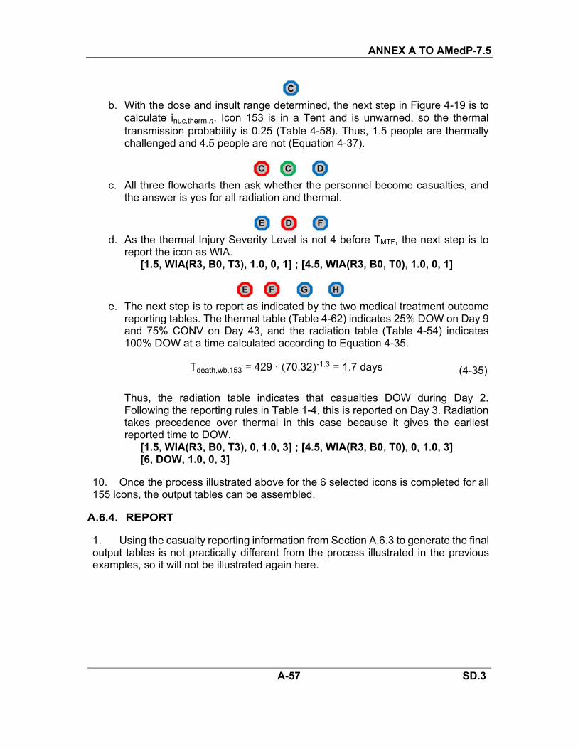
ANNEX A TO AMedP-7.5

A-57 SD.3

b. With the dose and insult range determined, the next step in Figure 4-19 is to

calculate inuc,therm,n. Icon 153 is in a Tent and is unwarned, so the thermal transmission probability is 0.25 (Table 4-58). Thus, 1.5 people are thermally challenged and 4.5 people are not (Equation 4-37).

c. All three flowcharts then ask whether the personnel become casualties, and

the answer is yes for all radiation and thermal.

d. As the thermal Injury Severity Level is not 4 before TMTF, the next step is to

report the icon as WIA. [1.5, WIA(R3, B0, T3), 1.0, 0, 1] ; [4.5, WIA(R3, B0, T0), 1.0, 0, 1]

e. The next step is to report as indicated by the two medical treatment outcome

reporting tables. The thermal table (Table 4-62) indicates 25% DOW on Day 9 and 75% CONV on Day 43, and the radiation table (Table 4-54) indicates 100% DOW at a time calculated according to Equation 4-35.

Tdeath,wb,153 = 429 · 70.32 -1.3 = 1.7 days (4-35)

Thus, the radiation table indicates that casualties DOW during Day 2. Following the reporting rules in Table 1-4, this is reported on Day 3. Radiation takes precedence over thermal in this case because it gives the earliest reported time to DOW. [1.5, WIA(R3, B0, T3), 0, 1.0, 3] ; [4.5, WIA(R3, B0, T0), 0, 1.0, 3] [6, DOW, 1.0, 0, 3]

10. Once the process illustrated above for the 6 selected icons is completed for all 155 icons, the output tables can be assembled.

A.6.4. REPORT

1. Using the casualty reporting information from Section A.6.3 to generate the final output tables is not practically different from the process illustrated in the previous examples, so it will not be illustrated again here.

ANNEX A TO AMedP-7.5

A-58 SD.3

Table A-25: Estimated Daily Number of New Nuclear Casualties*

Casualty Description Day 1 Day 2 Day 3 Day 4 Day 5 Day 6 Day 7Days 8–14

Days 15–30

Days 31+

New KIA (N) 21 0 0 0 0 0 0 0 0 0

New DOW (CRN) 0 266 47 27 17 12 2 67 75 7

Sum of New Fatalities 21 0 0 0 0 0 0 0 0 0

New WIA (Nuclear) 725 0 0 0 0 0 0 0 0 0

New CONV (Nuclear) 0 0 0 0 0 0 0 0 47 56

New RTD 0 0 0 0 0 0 0 0 94 0 * Estimate is based on Casualty Criterion WIA(1+), a PAR of 816, and FlagMT = Yes w/o G-CSF.

Table A-26: Estimated Personnel Status for Nuclear Casualties*

Casualty Description Day 1 Day 2 Day 3 Day 4 Day 5 Day 6 Day 7Days 8–14

Days 15–30

Days 31+

Fatalities

KIA—N 21 21 21 21 21 21 21 21 21 21 DOW—CRN 0 266 313 340 357 369 371 438 513 520

Sum of Fatalities 21 287 334 361 378 390 392 459 534 541

WIA

R0, B0, T1 94 140 140 140 140 140 140 140 0 0 R1, B0, T0 9 0 0 0 0 0 0 0 0 0

R1, B0, T1 47 0 0 0 0 0 0 0 0 0

R2, B0, T0 7 0 0 0 0 0 0 0 14 0

R2, B0, T1 7 14 14 14 14 14 14 14 0 0 R3, B0, T0 129 0 0 0 0 0 0 0 48 0

R3, B0, T1 57 176 145 137 128 118 116 80 0 0

R3, B0, T2 57 57 57 57 57 57 57 42 0 0

R3, B0, T3 78 55 47 28 20 18 18 2 2 0

R3, B2, T0 64 0 0 0 0 0 0 0 0 0 R3, B2, T1 0 8 0 0 0 0 0 0 0 0

R3, B2, T3 99 0 0 0 0 0 0 0 0 0

R3, B3, T0 51 0 0 0 0 0 0 0 0 0

R3, B3, T3 27 0 0 0 0 0 0 0 0 0

Sum of WIA 726 450 403 376 359 347 345 278 64 0

CONV

CONV (R) 0 9 9 9 9 9 9 9 55 110 CONV (R, T) 0 0 0 0 0 0 0 0 0 1

Sum of CONV 0 9 9 9 9 9 9 9 55 111

RTD

RTD 0 0 0 0 0 0 0 0 94 94 * Estimate is based on Casualty Criterion WIA(1+), a PAR of 816, and FlagMT = Yes w/o G-CSF.

ANNEX A TO AMedP-7.5

A-59 SD.3

A.7. NON-CONTAGIOUS BIOLOGICAL AGENT: B. ANTHRACIS

1. The following excerpt from Table 1-5 shows which sections of AMedP-7.5 explain how to complete the five major steps for an anthrax casualty estimate.

Agent, Effect, or Disease Five Steps

INPUT CHALLENGE RESPONSE/STATUS REPORT

Anthrax Ch. 2 Ch. 3 Sections 5.2.1 and 5.1.4 Ch. 6

2. In order to more easily follow along with the example, it is recommended that the reader print and have available for reference the following figures and tables: Figure 1-1, Figure 1-3, the annotated version of Figure 5-3 located on the next page, Table 5-4, Table 5-6 to Table 5-8, and Table A-1.

3. The red octagons containing a single letter in the annotated version of Figure 5-3 are user aids to help link the text later in the anthrax example to the various parts of the flowchart. Specifically, the red octagons are used to mark the beginning of the

text discussion related to the linked flowchart element. For example, the on the first line of Section A.7.2 indicates that the discussion of the calculation of the

Effective CBRN Challenge (Xanth,neff ) begins there; is linked to the calculation of

Xanth,neff because of its placement in the annotated version of Figure 5-3.

4. As noted in Table A-2, the anthrax example will illustrate the process for a casualty criterion of WIA(1+) and FlagMT = Yes. Further, as stated in Section A.2.1.6, this example will be different from the other five examples in that the forces will be modeled as initially not wearing their masks, but then donning their masks partway through the scenario. For simplicity, it is assumed that all personnel don masks at the same time: 15 minutes into the challenge.

A.7.1. INPUT

1. Two INPUTs not given in Section A.2 are needed: the CBRN Challenge per icon over time, and the vaccination status of each icon. Although it is unlikely in a real scenario, this example is based on the assumption of no vaccination (ρn = 0 for all n). If vaccination was included in the scenario, very few casualties would occur. The CBRN Challenge step is not associated with a red octagon because it occurs in the flowchart of Figure 1-3, which is “upstream” of Figure 5-3. Finally, as stated in Section 2.1.2, the CBRN Challenge must be generated independently of AMedP-7.5, using national tools.

2. The simulated attack comprised a person with a backpack sprayer containing 14 kg of B. anthracis, standing southwest of the airfield base. The backpack sprayer released B. anthracis (with an active fraction of 0.6) at a rate of 0.279972 kg/min over the course of 50 minutes, at a height of 2 meters. The simulated attack occurred at 2000 hours on cultivated terrain. Meteorological conditions were no cloud cover, wind at an average speed of about 2 m/s from the southwest toward the northeast, and an

ANNEX A TO AMedP-7.5

A-60 SD.3

average temperature of 20.7 °C. Figure A-6 is a qualitative depiction of the CBRN Challenge (cumulative) at the end of the simulation. Each filled red circle represents an icon, and the B. anthracis plume is depicted with colors indicating different amounts of CBRN Challenge (purple is low, red is high).

Figure 5-3 Annotated for Illustrative Example

3. To generate the quantitative input needed for AMedP-7.5, the CBRN Challenge per icon was extracted from HPAC in one-minute intervals. The extracted data for 7 selected icons are shown in Table A-27. Data are shown only for the three time points needed to complete the calculation of Effective CBRN Challenge. The table is in the CHALLENGE section (Section A.7.2) because it also includes all other information used to calculate Effective CBRN Challenge, and the final calculated values for each selected icon.

ANNEX A TO AMedP-7.5

A-61 SD.3

Figure A-6: B. anthracis (Anthrax) Attack on Task Force

A.7.2. CHALLENGE

1. As the IPE attribute for several of the icons does change over time, the sum in Equation 3-1 must have two terms. Thus, the application of Equation 3-1 for this example is:

Xanth,neff =

(Xanth,n,15 - Xanth,n,0) · Zn

APFanth,t<15,n

(Xanth,n,100 - Xanth,n,15) · Zn

APFanth,t≥15,n (3-1)

2. The values of Xanth,n,0, Xanth,n,15, and Xanth,n,100 are in the second through fourth columns of Table A-27. The APF is calculated per 2-2, with PFIPE,anth,n = 1 for t < 15, and the value indicated in the table for t ≥ 15. Details of the APF calculation are not repeated here because the process was illustrated in the GB example.

3. The value of Zn is determined by matching the specified Activity Level in Table A-1 with the corresponding breathing rate from Table 2-3.

4. Using the data in Table A-27 and the version of Equation 3-1, the Effective CBRN Challenge per icon may be calculated. Table A-27 contains the results. The results for all 155 icons are not shown, for brevity.

ANNEX A TO AMedP-7.5

A-62 SD.3

Table A-27: B. anthracis CBRN Challenge Data and Calculation of Effective CBRN Challenge for Selected Icons

Icon # (n) Xanth,n,tk [spores-min/m3]

at Time tk (min) Breathing Rate (Zn) (m3/min)

PFIPE,anth,n (tk ≥ 15

min)

PFV-SH,anth,n (all times)

Xanth,neff

[spores-min/m3] 0 15 100

8 0 2.99×104 5.66×105 0.03 1667 1 4.45×102 63 0 8.62×10-1 5.58×102 0.03 1667 1 1.91×10-2 73 0 4.13×108 1.87×109 0.03 1667 1.054 1.04×107 94 0 9.60×107 3.84×108 0.03 1667 1.054 2.47×106 98 0 1.55×107 6.09×107 0.03 1667 1.052 4.10×105 115 0 2.47×108 1.54×109 0.03 1 3000 1.54×104 116 0 1.14×108 7.79×108 0.03 1 3000 7.79×103

A.7.3. RESPONSE/STATUS

1. Figure 5-3 indicates that the next step is to assign each icon to a dose range. This is done simply by comparing the icon’s Xanth,n

eff to the values in Table 5-4.

2. Now, with Xanth,n

eff , in, and ρn available, and each icon assigned to a dose range, the next step is to estimate the populations of the EDR cohorts, using Equation 5-1. Section 5.2.1.3 also states that Equation 5-1 is applied separately to each dose range.

a. Thus, for example, every icon for which the following inequality is true will be used to calculate the population of ED: 104 < Xanth,n

eff ≤ 105. The example icons in Table A-27 were chosen to have one icon per dose range. The example calculations will be shown as if the 7 example icons were the only icons in the scenario. Thus, taking icon 115 as an example, the application of Equation 5-1 is:

E = 10 · 1 - 0 · pE Xanth,115eff

b. Table 5-8 indicates that the value of pE Xanth,115eff should be calculated using

Equation 5-32, which, for icon 115, is implemented via:

pE Xanth,155eff = Φ 0.79 · log10

1.54×104 spores

1.60×104 spores = 0.4948

c. Plugging pE Xanth,155eff back into the equation for E gives 4.948 individuals in

ED from icon 115. Expanding these calculations to all icons and all dose ranges gives the populations of all the EDR (see Table A-28), which are necessary for the remainder of the process diagrammed in Figure 5-3.

ANNEX A TO AMedP-7.5

A-63 SD.3

3. The casualty criterion is WIA(1+), so the next step is to report the daily number of WIA and WIA(2) to Equations 5-5 and 5-7. Using the EDR populations from Table A-28, the reporting information passed to the equations is: [0.547, WIA or WIA(2), Table 5-9A] ; [7.540, WIA or WIA(2), Table 5-9B] [30.977, WIA or WIA(2), Table 5-9C] ; [81.935, WIA or WIA(2), Table 5-9D] [124.152, WIA or WIA(2), Table 5-9E] ; [206.566, WIA or WIA(2), Table 5-9F] [70.315, WIA or WIA(2), Table 5-9G]

4. As the value of FlagMT is Yes, the next step in Figure 5-3 is to calculate the populations of the FDR,U, FDR,T-2, FDR,T-1, and SDR,T-1 cohorts. These calculations will not be shown here; the results are in given Table A-28. As stated in Table A-2, the value of dtrt-anth used to calculate the populations was 7 days.

Table A-28: Populations of Anthrax Cohorts Dose Range EDR FDR,U FDR,T-2 FDR,T-1 SDR,T-1

A 0.547 0.043 0.020 0.054 0.430 B 7.540 0.795 0.368 0.735 5.642 C 30.977 5.040 2.233 2.946 20.757 D 81.935 24.204 8.865 7.065 41.801 E 124.152 67.278 14.873 7.637 34.364 F 206.566 157.334 15.781 6.848 26.594 G 70.315 56.568 4.514 2.062 7.170

5. With the cohort populations calculated, the next step in Figure 5-3 is to report the daily number of casualties becoming WIA(4), using Table 5-10 and Table 5-12. The reporting information passed to Equation 5-7 is: [0.043, WIA(4), Table 5-10A] ; [0.795, WIA(4), Table 5-10B] [5.040, WIA(4), Table 5-10C] ; [24.204, WIA(4), Table 5-10D] [67.278, WIA(4), Table 5-10E] ; [157.334, WIA(4), Table 5-10F] [56.568, WIA(4), Table 5-10G] [0.020, WIA(4), Table 5-10A] ; [0.368, WIA(4), Table 5-10B] [2.233, WIA(4), Table 5-10C] ; [8.865, WIA(4), Table 5-10D] [14.873, WIA(4), Table 5-10E] ; [15.781, WIA(4), Table 5-10F] [4.514, WIA(4), Table 5-10G] [0.054, WIA(4), Table 5-12A] ; [0.735, WIA(4), Table 5-12B] [2.946, WIA(4), Table 5-12C] ; [7.065, WIA(4), Table 5-12D] [7.637, WIA(4), Table 5-12E] ; [6.848, WIA(4), Table 5-12F] [2.062, WIA(4), Table 5-12G] [0.430, WIA(4), Table 5-12A] ; [5.642, WIA(4), Table 5-12B] [20.757, WIA(4), Table 5-12C] ; [41.801, WIA(4), Table 5-12D] [34.364, WIA(4), Table 5-12E] ; [26.594, WIA(4), Table 5-12F] [7.170, WIA(4), Table 5-12G]

ANNEX A TO AMedP-7.5

A-64 SD.3

6. Following one flowchart branch, the next step is to report the daily number of DOW, using Table 5-11, Table 5-13, and Table 5-16. The reporting information passed to Equations 5-6 to 5-8 is: [0.043, DOW, Table 5-11A] ; [0.795, DOW, Table 5-11B] [5.040, DOW, Table 5-11C] ; [24.204, DOW, Table 5-11D] [67.278, DOW, Table 5-11E] ; [157.334, DOW, Table 5-11F] [56.568, DOW, Table 5-11G] [0.020, DOW, Table 5-16A] ; [0.368, DOW, Table 5-16B] [2.233, DOW, Table 5-16C] ; [8.865, DOW, Table 5-16D] [14.873, DOW, Table 5-16E] ; [15.781, DOW, Table 5-16F] [4.514, DOW, Table 5-16G] [0.054, DOW, Table 5-13A] ; [0.735, DOW, Table 5-13B] [2.946, DOW, Table 5-13C] ; [7.065, DOW, Table 5-13D] [7.637, DOW, Table 5-13E] ; [6.848, DOW, Table 5-13F] [2.062, DOW, Table 5-13G]

7. Following the other flowchart branch, the daily number becoming WIA(3) must be reported to Equation 5-7, then the daily number of CONV must be reported to Equations 5-6 to 5-8, then the daily number of RTD must be reported to Equations 5-6 to 5-8. For brevity, the reporting information is not stated here; it follows the pattern established above.

A.7.4. REPORT

1. Section A.7.3 stated some of the information that would be reported to Equations 5-5 to 5-8. This section will give a few examples of how that information is used to populate the output tables, and will show the completed output tables.

2. As an example of the use of Equation 5-5, consider the application to determine the number of new WIA on Day 2. Note that the “relevant cohorts” in Equation 5-5 are each of the seven EDR, and the values pulled from the PDT (Table 5-9) depend upon the dose range, as indicated by the reporting information listed under paragraph 2 of Section A.7.3.

NewWIA 2 = 0.547 · 0.0185 + 7.54 · 0.0216 + 30.977 · 0.0326 + 81.935 · 0.0793

+ 124.152 · 0.3779 + 206.566 · 0.2583 + 70.315 · 0.0002 = 107.97 108 (5-5)

The rate table (Table A-29) reports 108 casualties as new WIA on Day 2.

3. As an example of the use of Equation 5-6, consider the application to determine the number of new DOW on Day 7. The relevant cohorts are all F cohorts: the seven FDR,U, the seven FDR,T-2, and the seven FDR,T-1. The reporting information is listed under paragraph 5 of Section A.7.3. Note that the values pulled from the PDTs are

ANNEX A TO AMedP-7.5

A-65 SD.3

from the Day 6 row of each PDT.

NewDOW 7 = 0.043 · 0.0244 + 0.795 · 0.0325 + 5.040 · 0.0513 + 24.204 · 0.0985

+ 67.278 · 0.1863 + 157.334 · 0.1851 + 56.568 · 0.1638 + 0.020 · 0.0150 +

+ 0.368 · 0.0197 + 2.233 · 0.0312 + 8.865 · 0.0631 + 14.873 · 0.1416 +

+ 15.781 · 0.1893 + 4.514 · 0.1803 + 0.054 · 0.0028 + 0.735 · 0.0034 +

+ 2.946 · 0.0053 + 7.065 · 0.0120 + 7.637 · 0.0420 + 6.848 · 0.1348 +

+ 2.062 · 0.1618 = 61.8162 62

(5-6)

The rate table (Table A-29) reports 62 casualties as new DOW on Day 7.

4. As an example of Equation 5-7, consider the application to determine the totalnumber of WIA(4) on Day 5. Each of the seven dose ranges within the FDR,U, FDR,T-2, FDR,T-1, and SDR,T-1 are relevant as both “entering” and “exiting” cohorts. Rather than write out all the numbers, the following is a slightly shorter, and perhaps more instructive, version of Equation 5-7.

TotWIA(4) 5 = TotWIA(4) 4 +

FDR,U · PDT5-10 5 + FDR,T-2 · PDT5-10 5 + FDR,T-1 · PDT5-12 5 + SDR,T-1 · PDT5-12 5DR

-

FDR,U · PDT5-11 4 + FDR,T-2 · PDT5-16 4 + FDR,T-1 · PDT5-13 4 + SDR,T-1 · PDT5-13 5DR

-

(5-7)

5. As an example of Equation 5-8, consider the application to determine the totalnumber of DOW on Day 5. Each of the seven dose ranges within the FDR,U, FDR,T-2, and FDR,T-1 are relevant as “entering,” and there are no “exiting” cohorts.

TotDOW 5 = TotDOW 4 +

FDR,U · PDT5-11 4 + FDR,T-2 · PDT5-16 4 + FDR,T-1 · PDT5-13 4DR

(5-8)

6. To complete all entries in the reporting tables, Equations 5-5 to 5-8 must beapplied for every day for which the PDTs contain entries. The remainder of the calculations are not shown here. The results are given in Table A-29 and Table A-30. Note that the tables stop at Day 99+ even though some PDTs extend longer; this is because rounding to whole numbers causes no more change in casualty status to occur after Day 98.

ANNEX A TO AMedP-7.5

A-66 SD.3

Table A-29: Estimated Daily Number of New Anthrax Casualties* Casualty

Description Day 1 Day 2 Day 3 Day 4 Day 5 Day 6 Day 7

Days8–14

Days15–21

Days 22–28

Days29–35

Days36–42

Days43–70

Days71–77

Days78–84

Days85–91

Days92–98

Days99+

New DOW (B) 0 0 1 16 44 61 62 54–8 5–1 0 0 0 0 0 0 0 0 0 New WIA (Anthrax) 225 108 80 46 25 14 8 5–0 0 0 0 0 0 0 0 0 0 0

New CONV (Anthrax) 0 0 0 0 0 0 0 0 0–18 17–4 3–0 0 0 0 0 0 0 0

New RTD 0 0 0 0 0 0 0 0 0 0 0 0 0 0–3 7–13 10–1 1–0 0 * Estimate is based on Casualty Criterion WIA(1+), a PAR of 816, and dtrt-anth = 7 days.

Table A-30: Estimated Personnel Status for Anthrax Casualties*

Casualty Description

Day 1

Day 2

Day 3

Day4

Day5

Day6

Day7

Days 8–14

Days 15–21

Days 22–28

Days 29–35

Days 36–42

Days43–70

Days 71–77

Days78–84

Days 85–91

Days 92–98

Days99+

Fatalities

DOW (B) 0 0 1 17 60 121 183 327–369 374–384 384–385 385 385 385 385 385 385 385 385

WIA

Anthrax(2) 225 327 373 354 305 247 191 142–17 12–2 1–0 0 0 0 0 0 0 0 0 Anthrax(3) 0 0 0 0 0 3 10 22–111 118–78 62–9 7–1 1–0 0 0 0 0 0 0

Anthrax(4) 0 5 39 88 116 121 112 96–16 11–1 1–0 0 0 0 0 0 0 0 0

Sum of WIA 225 333 412 442 421 371 313 260–144 141–81 64–9 5–1 1–0 0 0 0 0 0 0

CONV

CONV (Anthrax) 0 0 0 0 0 0 0 0 0–56 73–127 130–136 136–137 137 137–134 127–36 26–4 3–1 0

RTD

RTD 0 0 0 0 0 0 0 0 0 0 0 0 0 0–3 10–101 111–133 134–136 136* Estimate is based on Casualty Criterion WIA(1+), a PAR of 816, and dtrt-anth = 7 days.

ANNEX A TO AMedP-7.5

A-67 SD.3

A.8. CONTAGIOUS BIOLOGICAL AGENT: V. MAJOR

1. The following excerpt from Table 1-5 shows which sections of AMedP-7.5 explain how to complete the five major steps for a smallpox (contagious) casualty estimate.

Agent, Effect, or Disease Five Steps

INPUT CHALLENGE RESPONSE/STATUS REPORT

Smallpox (non-contagious) Ch. 2 Ch. 3 Sections 5.2.9 and 5.1.4 Ch. 6 Smallpox (contagious) Ch. 2 Ch. 3 Sections 5.2.10 and 5.1.5 Ch. 6

2. In order to more easily follow along with the example, it is recommended that the reader print and have available for reference the following figures and tables:

a. For non-contagious and contagious: Figure 1-1, Figure 1-3, Table 5-76 to Table 5-78, Table A-1.

b. For non-contagious only: the annotated version of Figure 5-10 located on the next page.

c. For contagious only: Figure 5-2, Table 5-3, and Table 5-83.

3. The red octagons containing a single letter in the annotated version of Figure 5-10 are user aids to help link the text later in the non-contagious smallpox sections to the various parts of the flowchart. Specifically, the red octagons are used to mark the beginning of the text discussion related to the linked flowchart element. For

example, the on the first line of Section A.8.2 indicates that the discussion of the

calculation of the Effective CBRN Challenge (Xspox,neff ) begins there; is linked to

the calculation of Xspox,neff because of its placement in the annotated version of Figure

5-10.

4. As noted in Table A-2, the smallpox example will illustrate a smallpox casualty estimate for two cases. In one case, the casualty criterion is WIA(1+) and the non-contagious model will be used. In the other case, the casualty criterion is WIA(3+) and the contagious model will be used. In both cases, FlagMT = Yes and dvac-spox = day 12 (to model a scenario in which vaccination occurs in response to personnel becoming ill with smallpox, but it takes some time to ship the vaccines to the theatre of operations). The INPUT and CHALLENGE sections are the same for the non-contagious and contagious models, so they will not be repeated. However, the RESPONSE/STATUS and REPORT sections are separate for the non-contagious (Sections A.8.3 and A.8.4) and contagious (Sections A.8.5 and A.8.6) models.

ANNEX A TO AMedP-7.5

A-68 SD.3

Figure 5-10 Annotated for Illustrative Example

A.8.1. INPUT

1. The only INPUT needed that was not given in Section A.2 is the CBRN Challenge per icon over time. In addition to the value of dvac-spox, it is also necessary to know that all icons are assumed to have the same vaccination status, that is, they are unvaccinated before the attack, and all are vaccinated on day 12. If icons were instead vaccinated before the challenge, very few casualties would occur. The CBRN Challenge step is not associated with a red octagon on the non-contagious flowchart because it occurs in the flowchart of Figure 1-3, which is “upstream” of Figure 5-10. Finally, as stated in Section 2.1.2, the CBRN Challenge must be generated independently of AMedP-7.5, using national tools.

2. The simulated attack comprised a person with a backpack sprayer containing 14 kg of V. major, standing southwest of the airfield base. The backpack sprayer released V. major (with an active fraction of 0.6) at a rate of 0.279972 kg/min over the course of 50 minutes, at a height of 2 meters. The simulated attack occurred at 2000 hours on cultivated terrain. Meteorological conditions were no cloud cover, wind at an average speed of about 2 m/s from the southwest toward the northeast, and an average temperature of 20.7 °C. Figure A-7 is a qualitative depiction of the CBRN

ANNEX A TO AMedP-7.5

A-69 SD.3

Challenge (cumulative) at the end of the simulation. Each filled red circle represents an icon in the task force, and the V. major plume is depicted with colors indicating different amounts of CBRN Challenge (purple is low, red is high).

3. To generate the quantitative input needed for AMedP-7.5, the CBRN Challengeper icon was extracted from HPAC in one-minute intervals.

A.8.2. CHALLENGE

The other illustrative examples have demonstrated calculation of the Effective CBRN Challenge in sufficient detail that another example is not warranted here. The value of Xspox,n

eff per icon was estimated consistent with the method demonstrated in anthrax example, except that the full protection indicated in Table A-1 was modeled.

Figure A-7: V. major (Smallpox) Attack on Task Force

A.8.3. RESPONSE/STATUS—Non-Contagious Model

1. According to Figure 5-10, with Xspox,neff , in, and dvac-spox available, the next step is

to estimate the populations of the six cohorts, using Equations 5-3, 5-4, 5-72, and 5-73.

2. First, the populations of EU and EV are calculated using Equations 5-72 and

ANNEX A TO AMedP-7.5

A-70 SD.3

5-73. Determining pE Xspox,neff is relatively simple due to the threshold infectivity model

indicated in Table 5-78: if Xspox,neff ≥ 10 PFU, the value is 1, and if not, the value is 0.

Because applying the equations is simple and the application of similar equations has been demonstrated in Section A.7, an example for a single icon will not be shown. Rather, Table A-31 shows the final result.

3. Once the populations of the E cohorts have been determined, applying Equations 5-3 and 5-4 is also straightforward. Table A-31 indicates that the CFR to be applied to EU is 30% or 0.3, while the CFR for the EV cohort is 3% or 0.03.

Table A-31: Populations of Smallpox Cohorts Cohort Population

EU 79.335 EV 18.250 FU 23.800 FV 0.547 SU 55.534 SV 17.702

4. The casualty criterion is WIA(1+), so the next step in Figure 5-10 is to report the daily number of WIA and WIA(2) to Equations 5-5 and 5-7. The reporting information passed to the equations is: [79.335, WIA or WIA(2), Table 5-79] ; [18.250, WIA or WIA(2), Table 5-79]

5. The next step in Figure 5-10 is to report the daily number of WIA(3) and WIA(4) to Equation 5-7. The reporting information passed to the equation is: [55.534, WIA(3), Table 5-80] ; [17.702, WIA(3), Table 5-80] [23.800, WIA(4), Table 5-80] ; [0.547, WIA(4), Table 5-80]

6. Following one path in Figure 5-10, the next step is to report the daily number of DOW to Equations 5-5 and 5-7. The reporting information is: [23.800, DOW, Table 5-81] ; [0.547, DOW, Table 5-81]

7. Following the other path in Figure 5-10, the next steps are to report the daily number of CONV to Equation 5-7 and then the daily number of RTD to Equations 5-5 and 5-7. The reporting information is: [55.534, CONV, Table 5-81] ; [17.702, CONV, Table 5-81] [55.534, RTD, Table 5-82] ; [17.702, RTD, Table 5-82]

ANNEX A TO AMedP-7.5

A-71 SD.3

A.8.4. REPORT—Non-Contagious Model

1. Section A.8.3 stated some of the information that would be reported to Equations 5-5 to 5-8. This section will give a few examples of how that information is used to populate the output tables, and will show the completed output tables.

2. As an example of the use of Equation 5-5, consider the application to determine the number of new WIA on Day 11:

NewWIA 11 = 79.335 · 0.2066 + 18.250 · 0.2066 = 20.16 ≈ 20 (5-5)

The rate table (Table A-32) reports 20 casualties as new WIA on Day 11.

3. As an example of the use of Equation 5-6, consider the application to determine the number of new RTD on Day 32.

NewRTD 32 = PopSU · PDT5-82 31 + PopSV

· PDT5-81 31 =

55.534 · 0.0877 + 17.702 · 0.0877 = 6.42 ≈ 6 (5-6)

The rate table (Table A-32) reports 6 casualties as new RTD on Day 32.

4. As an example of Equation 5-7, consider the application to determine the total number of WIA(3) on Day 14.

TotWIA(3) 14 = TotWIA(3) 13 + PopSU · PDT5-80 14 PopSV

· PDT5-80 14

PopSU · PDT5-81 14 PopSV

· PDT5-81 14 =

16+ 55.534·0.1864+17.702·0.1864 - 55.534·0+17.702·0 = 29.65 ≈ 30

(5-7)

The personnel status table (Table A-33) reports 30 total casualties as WIA(3) on Day 14.

5. As an example of Equation 5-8, consider the application to determine the total number of DOW on Day 28.

TotDOW 28 = TotDOW 27 + PopFU · PDT5-81 27 PopFV

· PDT5-81 27

= 6 + 23.800 · 0.1034+ 0.547 · 0.1034 = 8.52 ≈ 9

(5-8)

The personnel status table (Table A-33) reports 9 total casualties as DOW on Day 28.

6. To complete all entries in the reporting tables, Equations 5-5 to 5-8 must be applied for every day for which the PDTs contain entries. The remainder of the calculations is not shown here. The results are given in Table A-32 and Table A-33. Note that the tables stop at Day 47+ even though some PDTs extend longer; this is because rounding to whole numbers causes no more change in casualty status to occur after Day 46.

ANNEX A TO AMedP-7.5

A-72 SD.3

Table A-32: Estimated Daily Number of New Smallpox Casualties*

Casualty Description Day ≤7

Day 8

Day9

Day10

Day11

Day12

Day13

Day14

Days15–17

Days 18–21

Days22–24

Days25–28

Days29–31

Days32–35

Days36–38

Days39–42

Days43–46

Days≥47

New DOW (B) 0 0 0 0 0 0 0 0 0 0 0–1 1–3 3–2 2–1 1–0 0 0 0 New WIA (Smallpox) 0 1 5 13 20 22 17 11 6–1 0 0 0 0 0 0 0 0 0

New CONV (Smallpox) 0 0 0 0 0 0 0 0 0 0 1–3 5–8 8–6 5–2 1 0 0 0

New RTD 0 0 0 0 0 0 0 0 0 0 0 0–1 2–5 6–8 7–5 4–1 1–0 0 * Estimate is based on Casualty Criterion WIA(1+), a PAR of 816, and dvac-spox = 12 days.

Table A-33: Estimated Personnel Status for Smallpox Casualties*

Casualty Description

Day ≤7

Day 8

Day 9

Day10

Day11

Day12

Day13

Day14

Days 15–17

Days 18–21

Days 22–24

Days 25–28

Days 29–31

Days32–35

Days 36–38

Days 39–42

Days 43–46

Days≥47

Fatalities

DOW (B) 0 0 0 0 0 0 0 0 0 0 0–1 2–9 12–17 19–23 24 24 24 24

WIA

Smallpox (2) 0 1 6 18 36 52 56 48 35–11 5–0 0 0 0 0 0 0 0 0 Smallpox (3) 0 0 0 0 2 7 16 30 44–64 69–72 72–66 62–39 31–18 13–4 2–1 1–0 0 0

Smallpox (4) 0 0 0 0 1 2 5 10 15–21 23–24 24–22 20–13 10–6 4–1 1–0 0 0 0

Sum of WIA 0 1 6 18 39 60 77 88 90–96 97–84 96–88 92–52 41–24 17–5 3–1 1–0 0 0

CONV

CONV (Smallpox) 0 0 0 0 0 0 0 0 0 0–1 2–7 12–30 35–37 35–20 15–8 5–1 1–0 0

RTD

RTD 0 0 0 0 0 0 0 0 0 0 0 0–1 3–11 17–41 48–59 63–69 70–71 71 * Estimate is based on Casualty Criterion WIA(1+), a PAR of 816, and dvac-spox = 12 days.

ANNEX A TO AMedP-7.5

A-73 SD.3

A.8.5. RESPONSE/STATUS—Contagious Model

1. The first step of applying the SEIRP model is to calculate the populations of the P, E1, and S cohorts on day 0. This is done using Equations 5-9 to 5-11, the implementations of which are not demonstrated because they are simple; the results are P 0 = 816, E1 0 = 201, and S 0 = 615.

2. The remainder of the model is simple in concept: once per day, execute Equations 5-12 to 5-31. As μE1 = 7 days, no changes will occur for the first 7 days; the populations of the P, E1, and S cohorts will remain as stated in the previous paragraph.

3. Recall that because dvac-spox = day 12, νon 12 = 1, and νon d for any other day = 0. As the prophylaxis is by vaccine, not drugs, νoff d = 0 for all days.

4. On Day 7, all individuals are still incubating, so the I and R cohorts still have zero population, and the S cohort still has 615 individuals. For the E cohorts:

E1 7 = 0 5-16

E2 7 = E1 6 · 1 - ρE · νon 6 201 · 1 - 0.85 · 0 = 201 5-17

5. As E1 7 = 0, E1 will remain at 0 until contagious spread begins to occur. The first day on which β(d) > 0 is Day 9, so E1 8 = E1 9 = 0. E1 8 being zero makes calculating E2 8 simpler because the second term in Equation 5-19 is zero:

E2 8 = E2 7 · 1-ρE· on 7 · 1-1

μE2

+ 0 = 210· 1 - 0.85·0 · 1 - 1

4.6 = 157.3 5-19

6. On Day 8, the first symptoms appear (people enter I1). Since MTI1 = 0 for smallpox (per Table 5-83) and I1 7 = 0, Equation 5-20 reduces to:

I1 8 = E2 7 · 1 - ρE·νon 7

μE2

= 201 · 1 - 0.85·0

4.6 = 43.70 5-20

7. Skipping to Day 12, the last day before vaccination affects the cohort populations: the cohort populations for Day 11 are the first step to calculating the Day 12 cohort populations: S(11) = 600.23, E1 11 = 14.35, E2 11 = 75.82, I1 11 = 66.93, I2 11 = 55.15, RDOW 11 = 1.05, RS 11 = 2.46, RRTD 11 = 0, and P(11) = 0. For brevity, the equations shown below will contain the actual numbers, rather than first showing the symbols and then showing the numbers. For the symbols, refer back to the original statement of the equations in Section 5.1.5.

ANNEX A TO AMedP-7.5

A-74 SD.3

a. Beginning with Equation 5-13, first calculate S(12):

S 12 =600.23· 1-0.95·0 · 1-0.752619· 0·66.93 + (1-0)·55.15

816+ 0·0=569.70 5-13

b. Next, use Equation 5-18 to calculate E1 12 :

E1 12 = 14.35 · 1 - 0.85 · 0 · 1 - 1

7600.23 · 1 - 0.95 · 0 · 0.752619 · 0 · 66.93 + (1-0) · 55.15

816 = 42.83

5-18

c. Next, use Equation 5-19 to calculate E2 12 :

E2 12 = 75.82 · 1 - 0.85· 0 · 1 - 1

4.6 +

14.35 · 1 - 0.85 · 0

7 = 61.39 5-19

d. Next, use Equation 5-20 to calculate I1 12 :

I1 12 = 66.93 · 1 - 1

3+

75.82 · 1 - 0.85·0

4.6 · 1 - 0 · 0 · 1 = 61.10 5-20

e. Next, use Equation 5-21 to calculate I2 12 :

I2 12 = 55.15 · 1 - 1

14 +

66.93

3 = 73.52 5-21

f. Next, use Equation 5-22 to calculate RDOW 12 .

RDOW 12 = 1.05 + 55.15

14 · 0.3 = 2.23 5-22

g. Next, use Equation 5-23 to calculate RS 12 .

RS 12 = 2.46 + 55.15

14 · 1 - 0.3 -

0

14 · 1 - 0.3 + 0 · 0 · 1

∙ 66.93· 1-1

3+

75.82· 1-0.85·0

4.6‐ 0·0·1 · 0· 1-

1

3+

0· 1-0.85·0

4.6 = 5.22

5-23

h. Finally, use Equation 5-24 to calculate RRTD 12 (not shown; value is 0).

8. To finish the example, the calculations for Day 13 are shown below.

S 13 = 569.70· 1-0.95·1 · 1-1.138454· 0·61.10 + (1-0)·73.52

816+ 0·0 = 25.56 5-13

ANNEX A TO AMedP-7.5

A-75 SD.3

E1 13 = 42.83 · 1 - 0.85 · 1 · 1 - 1

7569.70 · 1 - 0.95 · 1 · 1.138454 · 0 · 61.10 + (1-0) · 73.52

816 = 8.43

5-18

E2 13 = 61.39 · 1 - 0.85· 1 · 1 - 1

4.6 +

42.83 · 1 - 0.85 · 1

7 = 8.12 5-19

I1 13 = 61.10 · 1 - 1

3+

61.39 · 1 - 0.85·1

4.6· 1 - 0 · 0 · 1 = 42.74 5-20

I2 13 = 73.52 · 1 - 1

14 +

61.10

3 = 88.64 5-21

RDOW 13 = 2.23 + 73.52

14· 0.03 = 2.39 5-22

RS 13 = 5.22 + 73.52

14· 1 - 0.03 -

0

14· 1 - 0.03 0 · 0 · 1

∙ 61.10· 1-1

3+

61.39· 1-0.85·1

4.6‐ 0·0·1 · 0· 1-

1

3+

0· 1-0.85·0

4.6 = 10.31

5-23

9. After the calculations are repeated for all days of interest, the REPORT sectioncan be completed. The final day of interest is the day that β(d) goes to zero and stays there, plus μE1+μE2+μ1+μ2+μRS.

A.8.6. REPORT—Contagious Model

1. Following Table 5-3, it is straightforward to calculate the values to be used topopulate the output tables. Examples are not given here because the equations are either simpler than or very similar to those demonstrated in Section A.8.5. Note that the casualty criterion in this example is WIA(3+), so individuals do not become casualties when in Stage 1 of illness—only in Stage 2. The final results are shown in Table A-34 and Table A-35.

2. By comparing the DOW rows in the two tables, one can see that some problemsrelated to rounding have appeared. Rather than prescribe a method of accounting for rounding error in the methodology, the user may use any desired method of dealing with rounding errors.

ANNEX A TO AMedP-7.5

A-76 SD.3

Table A-34: Estimated Daily Number of New Smallpox Casualties*

Casualty Description Day≤8

Day 9

Day10

Day11

Day12

Day13

Day14

Days15–21

Days22–28

Days 29–35

Days36–42

Days43–49

Days50–56

Days57–63

Days64–70

Days71–77

Days78–99

Days≥100

New DOW (B) 0 0 0 1 1 0 0 0 0 0 0 0 0 0 0 0 0 0 New WIA (Smallpox) 0 15 21 23 22 20 14 10–3 3–2 2–1 1–0 0 0 0 0 0 0 0

New CONV (Smallpox) 0 0 1 2 3 5 6 7–6 6–5 4–3 3–2 2–1 1 1 1–0 0 0 0

New RTD 0 0 0 0 0 0 0 1–7 7–6 5–4 4–3 3–2 2–1 1 1 0 0 0 * Estimate is based on Casualty Criterion WIA(3+), a PAR of 816, and dvac-spox = 12 days.

Table A-35: Estimated Personnel Status for Smallpox Casualties*

Casualty Description

Day ≤8

Day 9

Day 10

Day11

Day12

Day13

Day14

Days15–21

Days22–28

Days 29–35

Days 36–42

Days 43–49

Days 50–56

Days 57–63

Days 64–70

Days 71–77

Days 78–99

Days≥100

Fatalities

DOW (B) 0 0 0 1 2 2 3 4 4–5 5–6 6–7 7 7 7 7 7 8 8

WIA

Smallpox (3) 0 10 24 39 51 68 77 72 69–55 53–40 38–28 26–18 17–11 11–7 7–4 4–3 2–1 0 Smallpox (4) 0 4 10 17 22 21 20 13 12–8 7–5 5–3 3–2 2–1 1 1–0 0 0 0 Sum of WIA 0 15 35 55 74 89 97 85 81–63 60–45 43–33 29–20 19–12 12–8 8–4 4–3 2–1 0

CONV

CONV (Smallpox) 0 0 1 2 5 10 16 33 32–25 24–18 17–13 12–8 8–5 5–3 3–2 2–1 1–0 0

RTD

RTD 0 0 0 0 0 0 0 30 37–74 80–108 112–132 135–149 151–160 161–167 168–171 172–174 174–177 178* Estimate is based on Casualty Criterion WIA(3+), a PAR of 816, and dvac-spox = 12 days.

ANNEX A TO AMedP-7.5

A-77 SD.3

INTENTIONALLY BLANK

ANNEX B TO AMedP-7.5

B-1 SD.3

ANNEX B REFERENCES

Baba, Anthony J., Brian R. Schallhorn, Steward Share, and Susan M. Gaspar. Incidence of Skin Burns under Contemporary Army Uniforms Exposed to Thermal Radiation from Simulated Nuclear Fireballs. HDL-TR-2084. Adelphi, MD: U.S. Army Laboratory Command, Harry Diamond Laboratories, December 1986.

Barss, Neil M., and Ronald L. Weitz. “Reconstruction of External Dose for Beta Radiation Sources of Nuclear Weapon Origin.” Health Physics 91, no. 4 (2006): 379–389.

Blewett, William K., Dennis W. Reeves, Victor J. Arca, David P. Fatkin, and Brenda P. Cannon. Expedient Sheltering in Place: An Evaluation for the Chemical Stockpile Emergency Preparedness Program. Aberdeen Proving Ground, MD: Edgewood Research Development and Engineering Center, June 1996.

Cerveney, T. J., T. J. MacVittie, and R. W. Young. “Acute Radiation Syndrome in Humans.” In Warfare, Weaponry, and the Casualty, Edited by Richard I. Walker and T. J. Cerveney, 15–36. Textbooks of Military Medicine. Falls Church, VA: Office of the Surgeon General, Department of the Army, 1996.

Defense Threat Reduction Agency (DTRA). Standard Method ED04 – Skin Dose from Dermal Contamination. Fort Belvoir, VA: DTRA, 31 January 2010.

Dolatshahi, F., D. C. Kaul, and W. A. Woolson. Technical and User’s Manual, Fortran Edition, Version 6 of Air Transport of Radiation (ATR6). SAIC-90/1507, DNA-TR-91-165. La Jolla, CA: Science Applications International Corporation, 1992.

Drake, M. K., M. P. Fricke, D. E. Groce, D. C. Kaul, C. J. Ridfleisch, J. B. Swenson, and W. A. Woolson. An Interim Report on Collateral Damage. DNA 4734Z. La Jolla, CA: Science Applications, Inc., October 1978. CB009013.

“Hazard Prediction and Assessment Capability.” Version 5.3.226 with Patch 3. Defense Threat Reduction Agency, 2015.

Eckerman, Keith F., and Jeffrey C. Ryman. External Exposure to Radionuclides in Air, Water, and Soil. Federal Guidance Report No. 12, EPA-402-R-93-081. Washington, DC: U.S. Environmental Protection Agency, September 1993.

International Atomic Energy Agency (IAEA). Dangerous Quantities of Radioactive Material. Vienna: IAEA, August 2006.

———. Generic Procedures for Assessment and Response During a Radiological Emergency. IAEA-TECDOC-1162. Vienna: IAEA, 2000.

ANNEX B TO AMedP-7.5

B-2 SD.3

Johnson, Ted. A Guide to Selected Algorithms, Distributions, and Databases Used in Exposure Models Developed by the Office of Air Quality Planning and Standards. Chapel Hill, NC: TRJ Environmental, Inc., 2002.

Layton, David W. “Metabolically Consistent Breathing Rates for Use in Dose Assessments.” Health Physics 64, no. 1 (1993): 23–36.

Levin, Sheldon G. The Effect of Combined Injuries from a Nuclear Detonation on Soldier Performance. Espanola, NM: Technical Southwest, Inc., 1993.

McClellan, Gene E., George H. Anno, and Leigh N. Matheson. Consequence Analytic Tools for NBC Operations Volume 3: Chemical Agent Exposure and Casualty Estimation. Alexandria, VA: Defense Special Weapons Agency, 1998.

McClellan, Gene E., David J. Crary, and Darren R. Oldson. Approximating the Probability of Mortality Due to Protracted Radiation Exposures. ARA-TR-08-SEASSP-17176-1. Arlington, VA: Applied Research Associates, Inc., 2008.

North Atlantic Treaty Organization (NATO). AAP-6: NATO Glossary of Terms and Definitions, STANAG 3680. Brussels, Belgium: NATO, April 2014.

———. AJMedP-1: Allied Joint Medical Planning Doctrine, STANAG 2542. Brussels, Belgium: NATO, November 2009.

———. AJMedP-7: Allied Joint Medical Doctrine for Support to CBRN Defensive Operations, STANAG 2596. Brussels, Belgium: NATO, August 2015.

———. AJP-3.8(A): Allied Joint Doctrine for CBRN Defence, STANAG 2451. Brussels, Belgium: NATO, March 2012.

———. AJP-4(A): Allied Joint Logistics Doctrine, STANAG 2182. Brussels, Belgium: NATO, March 2004.

———. AJP-4.10(B): Allied Joint Medical Support Doctrine, STANAG 2228. Brussels, Belgium: NATO, May 2015.

———. AJP-5: Allied Joint Doctrine for Operational-Level Planning, STANAG 2526. Brussels, Belgium: NATO, June 2013.

———. AMedP-7.6: Commander's Guide to Medical Support in Chemical, Biological, Radiological, and Nuclear Environments, STANAG 2873. Brussels, Belgium: NATO, anticipated 2016.

———. AMedP-13(A): NATO Glossary of Medical Terms and Definitions, STANAG 2409. Brussels, Belgium: NATO, 6 May 2011.

———. ATP-45(E): Warning and Reporting and Hazard Prediction of Chemical, Biological, Radiological and Nuclear Incidents (Operators Manual), STANAG

ANNEX B TO AMedP-7.5

B-3 SD.3

2103. Brussels, Belgium: NATO, January 2014.

Northrop, John A., ed. Handbook of Nuclear Weapon Effects: Calculational Tools Abstracted from DTRA’s Effects Manual One (EM-1). Ft. Belvoir, VA: Defense Threat Reduction Agency, 2002.

Park, J. H., J. D. Spengler, D. W. Yoon, T. Dumyahn, K. Lee, and H. Ozkaynak. “Measurement of Air Exchange Rate of Stationary Vehicles and Estimation of in-Vehicle Exposure.” Journal of Exposure Analysis and Environmental Epidemiology 8, no. 1 (1998): 65–78.

U.S. Army Chemical School (USACMLS). Potential Military Chemical/Biological Agents and Compounds. FM 3-11.9/MCRP 3-37.1B/NTRP 3–11.32/AFTTP(I) 3-2.55. Washington, DC: U.S. Government Printing Office, January 2005.

U.S. Army Nuclear and Chemical Agency (USANCA). Personnel Risk and Casualty Criteria for Nuclear Weapons Effects (PRCC). Springfield, VA: USANCA, June 1999.

ANNEX B TO AMedP-7.5

B-4 SD.3

INTENTIONALLY BLANK

AMedP-7.5

LOAA-1 SD.3

LIST OF ACRONYMS AND ABBREVIATIONS

AAP Allied Administration Publication AC Hydrogen cyanide ACH Air changes per hour AJP Allied Joint Publication AMedP Allied Medical Publication APF Aggregate Protection Factor BDO Battle dress overgarment BDU Battle dress uniform CAT Casualty category CBRN Chemical, biological, radiological, and nuclear CFU Colony forming unit CG Phosgene CK Cyanogen chloride Cl2 Chlorine ColPro Collective protection CONV Convalescent CRN Chemical, radiological, and nuclear Ct Concentration time DOW Died of wounds ECt50 Effective median dosage (concentration time) ED50 Median effective dose EEEV Eastern equine encephalitis virus GB Sarin G-CSF Granulocyte-colony stimulating factor Gy Gray H2S Hydrogen sulfide HD Distilled mustard HPAC Hazard Prediction and Assessment Capability hr Hour ID50 Median infectious dose; dose resulting in infection and illness

for 50% of the exposed population IPE Individual protective equipment J/cm2 Joule per square centimeter

AMedP-7.5

LOAA-2 SD.3

KIA Killed in action kg Kilogram kJ/m2 Kilojoule per square meter kPa Kilopascal

LD50 Median lethal dose; dose resulting in lethality for 50% of the exposed population

m Meter mg Milligram min Minute MTF Medical treatment facility

N/A Not applicable NATO North Atlantic Treaty Organization NBC Nuclear, biological, and chemical N.O.I. No observable injury

PAR Population at risk PDT Probability density table %BSA Percentage body surface area burned to second or third

degree level PFU Plaque forming units

RBE Relative biological effectiveness RDD Radiological dispersal device RTD Return to Duty

S/S Signs and symptoms SEB Staphylococcal enterotoxin B SEIRP Susceptible, Exposed and infected, Infectious, Removed, and

Prophylaxis efficacious SRD Standards Related Document STANAG NATO standardization agreement

TBq Terabecquerel (1012 becquerels)

VEEV Venezuelan equine encephalitis virus VX O-Ethyl-S-(2-diisopropylaminoethyl) methyl phosphonothiolate

WEEV Western equine encephalitis virus WIA Wounded in action WIA(1+) Wounded in action (Severity Level 1 (“Mild”) or greater) WIA(2+) Wounded in action (Severity Level 2 (“Moderate”) or greater) WIA(3+) Wounded in action (Severity Level 3 (“Severe”) or greater)

R E P O R T D O C U M E N T AT I O N P A G E Form Approved OMB No. 0704-0188

Public reporting burden for this collection of information is estimated to average 1 hour per response, including the time for reviewing instructions, searching existing data sources, gathering and maintaining the data needed, and completing and reviewing this collection of information. Send comments regarding this burden estimate or any other aspect of this collection of information, including suggestions for reducing this burden to Department of Defense, Washington Headquarters Services, Directorate for Information Operations and Reports (0704-0188), 1215 Jefferson Davis Highway, Suite 1204, Arlington, VA 22202-4302. Respondents should be aware that notwithstanding any other provision of law, no person shall be subject to any penalty for failing to comply with a collection of information if it does not display a currently valid OMB control number. PLEASE DO NOT RETURN YOUR FORM TO THE ABOVE ADDRESS.

1 . R E P O R T D A T E ( D D - M M - Y Y )

December 20152 . R E P O R T T Y P E

Final3 . D AT E S C O V E R E D ( F r o m – To )

4 . T I T L E A N D S U B T I T L E 5 a . C O N T R A C T N O .

HQ0034-14-0001 NATO Allied Medical Publication 7.5 Study Draft 3 (AMedP-7.5 SD.3), “NATO Planning Guide for the Estimation of CBRN Casualties”

5 b . G R A N T N O .

5 c . P R O G R A M E L E M E N T N O ( S ) .

6 . A U T H O R ( S )Carl A. CurlingSean M. Oxford

5 d . P R O J E C T N O .

5 e . TA S K N O .

CA-6-3079 5 f . W O R K U N I T N O .

7 . P E R F O R M I N G O R G A N I Z A T I O N N A M E ( S ) AN D A DD R E S S ( E S )Institute for Defense Analyses4850 Mark Center DriveAlexandria, VA 22311-1882

8 . P E R F O R M I N G OR G A N I Z A T I O N R E P O R T NO .IDA Paper NS P-5308Log: H 15-001016

9 . S P O N S O R I N G / M O N I T O R I N G A G E N C Y N A M E ( S ) A N D A D D R E S S ( E S )

Office of the Surgeon General of the Army Joint Requirements Office-CBRN DefenseATTN: DASG-HCO (G-34) (JRO-CBRND) 7700 Arlington Blvd, Ste 5143 Joint Chiefs of Staff/J8 Falls Church, VA 22042-5143 8000 Joint Staff Pentagon, Room 1D958

Washington, DC 20318-8000

1 0 . S P O N S OR ’S / M O N I T O R ’ S A C R O N Y M ( S )

OTSG/JRO-CBRND, J-8

11 . S P O N S O R ’S / M O N I T OR ’ S R E P O R T N O ( S ) .

1 2 . D I S T R I B U T I O N / AV A I L A B I L I T Y S T A T E M E N T Approved for public release; distribution is unlimited.

1 3 . S U P P L E M E N T A R Y N O T E S

1 4 . A B S T R A C T This document is the third in a series of developmental draft documents leading to AMedP-7.5(A), the next iteration of the NATO CBRN casualty estimation methodology. This document presents the methodology as comprising five components—user input, estimation of the CBRN challenge, estimation of human response, casualty estimation, and reporting. This document fully describes the required inputs, the method of calculating the CBRN challenge, and the estimation and reporting of human response and casualties, including a dedicated section for each agent/effect describing how to estimate human response and casualties from that specific agent/effect. The methodology includes 12 chemical agents, 17 biological agents, nuclear effects, radiological dispersal device isotopes, and radiological fallout. To increase user-friendliness, each dedicated section contains a flowchart for that agent/effect instructing the user on which equations and lookup tables should be used, and the sequence in which they should be used; Appendix A contains illustrative examples for each of the major types of agent or effect. Although this is a Study Draft, it is envisioned as the final product, other than any changes required as part of the NATO review process.

1 5 . S U B J E C T T E R M S

CBRN, modeling, casualty estimation, medical planning, NATO, medical, doctrine, AMedP-7.5

1 6 . S E C U R I T Y C L A S S I F I C A T I O N O F :

1 7 . L I M I T A T I ON O F AB S T R A C T

U

1 8 . N O . O F P A G E S

338

1 9 a . N A M E O F R E S P O N S I B L E P E R S O N

Stewart, Harrya . R E P O R T

U

b . AB S T R A C T

U

c . T H I S P A GE

U

1 9 b . T E L E P H O N E N U M B E R ( I n c l u d e A r e a C o d e ) (703) 681-8188

Standard Form 298 Back (Rev. 8/98)

INTENTIONALLY BLANK

The information contained in this document shall not be released to a nation outside of NATO without following procedures contained in C-M(2002)60.