natural gas and electricity optimal power flow by seungwon an bachelor of
TRANSCRIPT

NATURAL GAS AND ELECTRICITY OPTIMAL POWER FLOW
By
SEUNGWON AN
Bachelor of EngineeringKorea Maritime University
Pusan, KoreaFebruary, 1991
Master of EngineeringOklahoma State University
Stillwater, OklahomaMay, 1999
Submitted to the Faculty of theGraduate College of the
Oklahoma State Universityin partial fulfillment ofthe requirements for
the Degree ofDOTOR OF PHILOSOPHY
May, 2004

NATURAL GAS AND ELECTRICITY OPTIMAL POWER FLOW
Thesis Approved:
Thesis Advisor
Dean of the Graduate College
ii

Acknowledgment
I would like to express my sincere appreciation to my advisor Dr. Thomas W.
Gedra for his intelligent supervision, friendship and confidence in me. I wish to thank
the other members of my doctoral committee, Dr. Ramakumar, Dr. Yen and Dr.
Misawa for their assistance throughout this work. I would like to give very special
thanks to Dr. Ramakumar for his continuous guidance during my study at OSU.
I wish to take this opportunity to express my gratitude to Mr. Lee Clark for his
assistance and encouragement in all aspects of my work. I wish to express my sincere
gratitude to the School of Electrical and Computer Engineering for providing me with
this research opportunity and generous financial support.
I am deeply indebted to all members of the Korean Catholic Community at Still-
water for their spiritual support. Especially, I would like to thank Mr. Hyunwoong
Hong and Mrs. Eunjoo Kang for their brotherhood.
I am deeply grateful to my wife, Misook Kim, for her patience and to our twin
boys, Clemens and Martino for their existence. My final appreciation goes to my
parents and brothers for their enduring love, support and encouragement.
iii
TABLE OF CONTENTS
1 INTRODUCTION . . . . . . . . . . . . . . . . . . . . . . . . . . . . . . . 1
2 AC LOADFLOW . . . . . . . . . . . . . . . . . . . . . . . . . . . . . . . . 6
2.1 Flows on Transmission Systems . . . . . . . . . . . . . . . . . . . . . 6
2.2 Loadflow Problem Statement . . . . . . . . . . . . . . . . . . . . . . . 10
2.3 Newton-Raphson Method . . . . . . . . . . . . . . . . . . . . . . . . 13
3 ECONOMIC DISPACTH . . . . . . . . . . . . . . . . . . . . . . . . . . . 17
3.1 Lossless Economic Dispatch . . . . . . . . . . . . . . . . . . . . . . . 18
3.2 Economic Dispatch with Transmission Losses . . . . . . . . . . . . . . 22
4 OPTIMAL POWER FLOW AND SOLUTION METHODS . . . . . . . . . 25
4.1 OPF by Newton’s Method . . . . . . . . . . . . . . . . . . . . . . . . 27
4.2 Primal-Dual Interior-Point (PDIP) Method . . . . . . . . . . . . . . . 31
5 NATURAL GAS FLOW MODELING . . . . . . . . . . . . . . . . . . . . 39
5.1 Elements of Natural Gas Transmission Network . . . . . . . . . . . . 40
5.2 Network Topology . . . . . . . . . . . . . . . . . . . . . . . . . . . . 41
5.3 Matrix Representations of Network . . . . . . . . . . . . . . . . . . . 43
5.4 Flow Equation . . . . . . . . . . . . . . . . . . . . . . . . . . . . . . . 43
5.5 Compressor Horsepower Equation . . . . . . . . . . . . . . . . . . . . 45
5.6 Conservation of Mass Flow . . . . . . . . . . . . . . . . . . . . . . . . 46
6 NATURAL GAS LOADFLOW . . . . . . . . . . . . . . . . . . . . . . . . 49
6.1 Loadflow Problem Statement . . . . . . . . . . . . . . . . . . . . . . . 50
6.2 Loadflow without Compressors . . . . . . . . . . . . . . . . . . . . . . 52
6.3 Loadflow with Compressors . . . . . . . . . . . . . . . . . . . . . . . 53
iv

7 UPFC MODELING FOR STEADY-STATE ANALYSIS . . . . . . . . . . 57
7.1 Operating Principles . . . . . . . . . . . . . . . . . . . . . . . . . . . 58
7.2 Uncoupled Model . . . . . . . . . . . . . . . . . . . . . . . . . . . . . 59
7.3 Ideal Transformer Model . . . . . . . . . . . . . . . . . . . . . . . . . 62
7.4 UPFC in a Transmission Line . . . . . . . . . . . . . . . . . . . . . . 65
8 GAS AND ELECTRICITY OPTIMAL POWER FLOW . . . . . . . . . . 69
8.1 Gas and Electric Combined Network . . . . . . . . . . . . . . . . . . 69
8.2 Gas and Electricity Optimal Power Flow . . . . . . . . . . . . . . . . 70
8.2.1 Cost, Benefit, and Social Welfare . . . . . . . . . . . . . . . . 71
8.2.2 Constraints . . . . . . . . . . . . . . . . . . . . . . . . . . . . 74
9 OPTIMAL LOCATION OF A UPFC IN A POWER SYSTEM . . . . . . . 79
9.1 Optimal Power Flow with UPFC . . . . . . . . . . . . . . . . . . . . 79
9.2 First-Order Sensitivity Analysis . . . . . . . . . . . . . . . . . . . . . 81
9.3 Second-Order Sensitivity Analysis . . . . . . . . . . . . . . . . . . . . 84
9.4 Estimation of Incremental Value . . . . . . . . . . . . . . . . . . . . . 87
10 RESULTS . . . . . . . . . . . . . . . . . . . . . . . . . . . . . . . . . . . . 88
10.1 Result of Sensitivity Analysis . . . . . . . . . . . . . . . . . . . . . . 88
10.2 Result of GEOPF . . . . . . . . . . . . . . . . . . . . . . . . . . . . . 92
10.2.1 Test System I . . . . . . . . . . . . . . . . . . . . . . . . . . . 93
10.2.2 Test System II . . . . . . . . . . . . . . . . . . . . . . . . . . 95
11 CONCLUSIONS AND FUTURE WORK . . . . . . . . . . . . . . . . . . . 101
BIBLIOGRAPHY . . . . . . . . . . . . . . . . . . . . . . . . . . . . . . . . . 104
A DERIVATIVES REQUIRED FOR GEOPF . . . . . . . . . . . . . . . . . 108
A.1 Electric Networks . . . . . . . . . . . . . . . . . . . . . . . . . . . . . 108
A.2 Gas Network . . . . . . . . . . . . . . . . . . . . . . . . . . . . . . . 115
A.3 Objective Function of GEOPF . . . . . . . . . . . . . . . . . . . . . . 119
B DERIVATIVES REQUIRED FOR UPFC SENSITIVITIES . . . . . . . . . 120
v

C INPUT DATA FILE FORMAT . . . . . . . . . . . . . . . . . . . . . . . . 130
C.1 IEEE Common Data Format . . . . . . . . . . . . . . . . . . . . . . . 130
C.2 Generator Data . . . . . . . . . . . . . . . . . . . . . . . . . . . . . . 133
C.3 Electricity Load Data . . . . . . . . . . . . . . . . . . . . . . . . . . . 134
C.4 Natural Gas Common Data Format . . . . . . . . . . . . . . . . . . . 135
C.5 Natural Gas Load Data . . . . . . . . . . . . . . . . . . . . . . . . . . 137
C.6 Natural Gas Source Data . . . . . . . . . . . . . . . . . . . . . . . . . 138
D MATLAB CODE . . . . . . . . . . . . . . . . . . . . . . . . . . . . . . . . 146
D.1 GEOPF . . . . . . . . . . . . . . . . . . . . . . . . . . . . . . . . . . 146
D.2 Base Case OPF with Sensitivity Analysis . . . . . . . . . . . . . . . . 157
D.3 OPF with a UPFC . . . . . . . . . . . . . . . . . . . . . . . . . . . . 167
vi
LIST OF FIGURES
1.1 Monthly natural gas price trends at AECO hub in Canada . . . . . . 2
1.2 Average Virginia mine coal price (1975-2000, Virginia) . . . . . . . . 3
2.1 Bus i and connection to transmission system . . . . . . . . . . . . . . 7
4.1 Effect of barrier term . . . . . . . . . . . . . . . . . . . . . . . . . . . 33
4.2 Graphical representation of central path . . . . . . . . . . . . . . . . 37
5.1 Pipeline network representation . . . . . . . . . . . . . . . . . . . . . 40
5.2 Graph of the gas network . . . . . . . . . . . . . . . . . . . . . . . . . 41
7.1 General UPFC scheme . . . . . . . . . . . . . . . . . . . . . . . . . . 58
7.2 Proposed UPFC model in a transmission line . . . . . . . . . . . . . . 59
7.3 Phasor diagram of UPFC input-output voltages and currents . . . . . 60
7.4 Uncoupled UPFC model in a transmission line. . . . . . . . . . . . . 61
7.5 UPFC ideal transformer model . . . . . . . . . . . . . . . . . . . . . 62
7.6 Simplified UPFC circuit . . . . . . . . . . . . . . . . . . . . . . . . . 64
7.7 Cascaded transmission line with a UPFC . . . . . . . . . . . . . . . . 66
8.1 Combined natural gas and electricity network . . . . . . . . . . . . . 70
10.1 Diagram of 5-bus subset of IEEE 14-bus system . . . . . . . . . . . . 88
10.2 Marginal and incremental values for 5-bus system . . . . . . . . . . . 89
10.3 Marginal and incremental values for IEEE 14-bus system . . . . . . . 90
10.4 Marginal and incremental values for IEEE 30-bus system . . . . . . . 91
vii
10.5 Combined gas and electric network . . . . . . . . . . . . . . . . . . . 92
10.6 SW losses due to non-integrated operation for test system I . . . . . . 96
10.7 Combined gas and electric network . . . . . . . . . . . . . . . . . . . 97
10.8 SW losses due to non-integrated operation for test system II . . . . . 98
viii
LIST OF TABLES
10.1 Real power generation, line loss and incremental value . . . . . . . . . 89
10.2 GEOPF results for test system I . . . . . . . . . . . . . . . . . . . . . 99
10.3 GEOPF results for test system II . . . . . . . . . . . . . . . . . . . . 100
ix

CHAPTER 1
INTRODUCTION
Restructuring of natural gas and electric industries, both known as network industries,
and deregulation of their products have been undertaken in the U.S. to minimize
the social inefficiency incurred by regulated monopolies when natural monopoly has
disappeared from their technologies [1]. Due to the successful deregulation of the
natural gas market, the wellhead price of natural gas declined by 44 % between 1983
and 1997.
Electric power generation technologies utilizing natural gas are generally less
capital-intensive and often more technically efficient than other alternatives. Thus,
natural gas is playing an important role in electric power generation since 1990 par-
tially due to incentives of the Clean Air Act Amendments (CAAA) of 1990. Since
1997, more than 120 GW of new capacity has been added by merchant energy com-
panies at a lower cost per installed MW and with shorter construction times than
in the past [2]. Most of this new generation is fueled by natural gas. However, due
to the lack of financial instruments to lock in future prices to reduce price risk, the
large increase in natural gas prices, and excess reserve margins, more than 110 GW of
installed capacity belongs to entities that have below-investment-grade credit ratings
(i.e., junk bonds) [2]. Thus, we have been experiencing large price volatility in major
natural gas markets while price volatility in electric markets has declined steadily
over the past three years [2]. In addition, the floor price for natural gas in summer
1
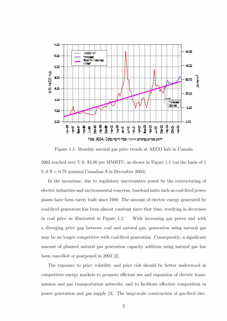
Figure 1.1: Monthly natural gas price trends at AECO hub in Canada
2003 reached over U.S. $4.00 per MMBTU, as shown in Figure 1.1 (on the basis of 1
U.S $ = 0.75 nominal Canadian $ in December 2003).
In the meantime, due to regulatory uncertainties posed by the restructuring of
electric industries and environmental concerns, baseload units such as coal-fired power
plants have been rarely built since 1990. The amount of electric energy generated by
coal-fired generators has been almost constant since that time, resulting in decreases
in coal price as illustrated in Figure 1.2. With increasing gas prices and with
a diverging price gap between coal and natural gas, generation using natural gas
may be no longer competitive with coal-fired generation. Consequently, a significant
amount of planned natural gas generation capacity addition using natural gas has
been cancelled or postponed in 2003 [2].
The exposure to price volatility and price risk should be better understood in
competitive energy markets to promote efficient use and expansion of electric trans-
mission and gas transportation networks, and to facilitate effective competition in
power generation and gas supply [3]. The large-scale construction of gas-fired elec-
2

Figure 1.2: Average Virginia mine coal price (1975-2000, Virginia)
tric generation, combined with electric power restructuring, is expected to create an
even greater convergence between electricity and natural gas markets. Lack of fuel
diversity (i.e., excessive dependence on natural gas with volatile prices, as opposed to
coal, especially newer “clean coal” technology) will likely increase volatility of gas and
electric prices, even if the price of coal is lower and less volatile. Therefore, viewing
these markets separately without recognizing their increasing convergence is myopic
at best, and disastrous at worst.
Economic forces in energy markets have been driving not only the optimal oper-
ation of energy networks but also efficient price-based system planning. The unified
power flow controller (UPFC) is one of the most technically promising devices in the
Flexible AC Transmission System (FACTS) family [4, 5, 6, 7]. It has the capability to
control both voltage magnitude and phase angle, and can also independently provide
(positive or negative) reactive power injections. However, it cannot be installed in
all possible transmission lines due to its high capital cost. Thus, a need exists for
developing a cost-benefit analysis technique to determine if installation of a UPFC
3

would be beneficial and the best location to install the UPFC. In principle, determin-
ing the optimal location for a UPFC is simple. For each possible location, we place
a UPFC in the power system model and calculate the cost savings with respect to a
base case (with no new UPFC installed). The operating cost at each time throughout
the year and for each potential location is determined using an optimal power flow
(OPF) program. However, the computational burden of evaluating this annual value
for every possible line is immense because an OPF problem must be solved for each
possible UPFC location and at each of several time periods. Therefore, an efficient
screening technique is desired to identify the most promising locations so that at each
point in time throughout the year, the exhaustive calculations described above do not
have to be carried out for every location that is a candidate for installing the UPFC.
In this research, we introduce fundamental natural gas modeling for steady-state
analysis, and propose general formulations to solve a combined natural gas and elec-
tric optimal power flow (GEOPF). In addition, a screening technique is developed
for greatly reducing the computation involved in determining the optimal UPFC lo-
cation in a large power system. This technique requires running only one optimal
power flow (OPF) to obtain UPFC sensitivities for all possible transmission lines. To
implement the screening technique, we develop a new mathematical model of UPFC
under steady-state, consisting of an ideal transformer with a complex turns ratio and
a variable shunt admittance.
We begin by reviewing basic concepts which describe power flows in power systems.
Economic dispatch is discussed next, followed by the introduction of the optimal
power flow concept and its solution methodology. A GEOPF model is described in
detail after the introduction of natural gas network modeling. A screening technique
based on sensitivity analysis is discussed next and a new UPFC model is described.
The GEOPF model has been successfully applied to two test cases: a 15-node gas
network with (i) a 5-bus electric network and (ii) a 9-bus electric network. The
4

screening technique (electricity only) has also been implemented in a 5-bus system
and IEEE 14- and 30-bus systems. Discussions of results are presented in Chapter
10.
5

CHAPTER 2
AC LOADFLOW
Electric loadflow problems are solved routinely to study power systems under both
normal operating conditions and under various contingencies using predicted data or
to analyze “what if” scenarios. It is also of great importance in power system planning
for future expansion. The principal information obtained from loadflow analysis is
the magnitude and phase angle of the voltage at each bus. Using these values, we can
calculate real and reactive power flows in transmission lines and transformers, and
line losses.
In this chapter, we describe the formulation of the bus admittance (Ybus) matrix,
which represents a transmission line network, and explain how complex power injec-
tions into a network are related to the bus voltage magnitudes and angles. Then, we
construct the loadflow problem and discuss some of its characteristics.
2.1 Flows on Transmission Systems
Consider a network of transmission lines connecting a set of buses in a power trans-
mission system. We will find out the relationship between complex power and current
injections into the transmission system and the phasor voltages at each bus. Figure
2.1 [8] shows connections to a transmission system at bus i. The double-subscript
notation Sik and ~Iik, for k 6= i, indicates complex power or phasor current (respec-
6
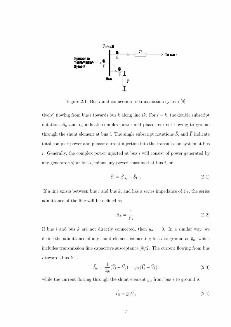
Figure 2.1: Bus i and connection to transmission system [8]
tively) flowing from bus i towards bus k along line ik. For i = k, the double subscript
notations Sii and ~Iii indicate complex power and phasor current flowing to ground
through the shunt element at bus i. The single subscript notations Si and ~Ii indicate
total complex power and phasor current injection into the transmission system at bus
i. Generally, the complex power injected at bus i will consist of power generated by
any generator(s) at bus i, minus any power consumed at bus i, or
Si = SGi− SDi
. (2.1)
If a line exists between bus i and bus k, and has a series impedance of zik, the series
admittance of the line will be defined as
yik =1
zik
. (2.2)
If bus i and bus k are not directly connected, then yik = 0. In a similar way, we
define the admittance of any shunt element connecting bus i to ground as yii, which
includes transmission line capacitive susceptance jb/2. The current flowing from bus
i towards bus k is
~Iik =1
zik
(~Vi − ~Vk) = yik(~Vi − ~Vk), (2.3)
while the current flowing through the shunt element yii from bus i to ground is
~Iii = yii~Vi, (2.4)
7

where ~Vi denotes the phasor voltage at bus i. If the total number of buses is n, the
total current injected into the power transmission system at bus i is
~Ii = yii~Vi +
n∑k=1k 6=i
yik
(~Vi − ~Vk
), (2.5)
or, collecting the ~Vi terms,
~Ii = ~Vi
n∑
k=1
yik −n∑
k=1k 6=i
yik~Vk. (2.6)
The right side of the above equation motivates the following definition:
Yii =n∑
k=1
yik, (2.7)
Yik = −yik, i 6= k. (2.8)
With this definition, we can write
~Ii =n∑
k=1
Yik~Vk. (2.9)
In matrix form, the definitions in equations (2.7) and (2.8) can be written as
Ybus =
y11 + · · · y1n −y12 · · · −y1n
−y21 y21 + · · · y2n · · · −y2n
.... . .
...
−yn1 −yn2 · · · yn1 + · · · ynn
.
In words, the diagonal element ii of the Ybus matrix consists of the sum of all admit-
tances connected to bus i (whether they are series admittances connecting to another
bus or are shunt admittances), while the off-diagonal element ik is the negative of the
series admittance connecting bus i to bus k. In the case that there is no transmission
line connecting bus i with bus k, yik = 0 as mentioned above. Likewise, yii = 0 if
no shunt element is present between bus i and ground. Note that, since the series
admittance yik connecting bus i to bus k is the same as that connecting bus k to bus i,
8
we have yik = yki, so that the matrix Ybus is symmetrical, assuming no phase-shifting
elements, which we have implicitly done.
If we define the bus voltage and bus current injection vectors as
~V =
~V1
~V2
...
~Vn
and ~I =
~I1
~I2
...
~In
,
then we can write equation (2.9) in matrix-vector form as
~I = Ybus~V. (2.10)
The matrix Ybus is called the bus admittance matrix, since it relates the bus voltages
and the bus current injections.
The complex power injection at bus i can be written in terms of Ybus matrix
elements as
Si = ~Vi~I∗i = ~Vi
n∑
k=1
Y ∗ik
~V ∗k , (2.11)
= Vi
n∑
k=1
VkYike(θi−θk−δik),
where
~Vi = Vi∠θi, ~Vk = Vk∠θk, and
Yik = Gik + jBik = Yik∠δik.
We can split equation (2.12) into real and reactive parts, in terms of the bus voltage
magnitudes {Vi, i = 1, . . . , n} and bus voltage angles {θi, i = 1, . . . , n}. Then the
real and imaginary parts of equation (2.12) become
Pi(~V) =n∑
k=1
ViVkYik cos(θi − θk − δik), (2.12)
Qi(~V) =n∑
k=1
ViVkYik sin(θi − θk − δik). (2.13)
9
The real and reactive power injections at bus i need to satisfy the following conditions:
PGi− PLi
= Pi(~V), i = 1, . . . , n, (2.14)
QGi−QLi
= Qi(~V), i = 1, . . . , n, (2.15)
where
PGi= real power generation at bus i,
PLi= real power load at bus i,
QGi= reactive power generation at bus i,
QLi= reactive power load at bus i.
We can rewrite equations (2.12), (2.12) and (2.13) in matrix form as
S =
S1
S2
...
Sn
=
~V1~I∗1
~V2~I∗2...
~Vn~I∗n
= diag{~V}~I∗ = diag{~I∗}~V, (2.16)
P = real(S), (2.17)
Q = imag(S), (2.18)
where diag{~V} denotes the diagonal matrix with the elements of the vector ~V on its
diagonal.
2.2 Loadflow Problem Statement
Since the loadflow solution is a prerequisite for many other analytical studies, it is
necessary to mathematically state the problem to prepare the ground for the estab-
lishment of its links to economic dispatch and optimal power flow. The loadflow
problem is stated below [8, 9, 10]:
10

• Given a power system described by a Ybus matrix, and given a subset of bus
voltage magnitudes, bus voltage angles, and real and reactive power bus injec-
tions,
• Determine the other voltage magnitudes and angles and real and reactive power
injections.
More precisely, two of the four quantities Vi, θi, Pi, and Qi at each bus are specified,
and the other two are to be determined. Each bus is classified based on the two
known quantities, as follows:
• PV bus, or generator bus, or voltage-controlled bus. For a bus i of this type,
we assume that we know the real power injection Pi and the voltage magnitude
Vi. This is because the real power generation can be controlled by adjusting the
prime mover input, and the voltage magnitude can be controlled by adjusting
the generator field current. However, certain buses without generators may have
some means of voltage support at that bus (such as a synchronous condenser,
capacitor banks, or a static VAr compensator).
• PQ bus, or load bus. For a non-generator bus i, we assume that we know the
real and reactive power injections Pi and Qi, and the bus voltage magnitude Vi
and angle θi are to be determined. In practice, only real power load is known
and the reactive power load is calculated based on an assumed power factor by
Qi = QGi− PLi
p.f.i
√1− p.f.2i .
We assume that a load is characterized by its constant complex power demand
(which does not depend on the bus voltage Vi, as opposed to assuming that the
load is a constant current or constant impedance load in which case the complex
power demand would depend on the bus voltage Vi.)
11

In fact, solving the loadflow problem with buses of only these two types is not in
general possible. The first reason is that, in the loadflow equations, the bus voltage
angles never appear by themselves, but instead appear only as angle differences of the
form θi − θk. Therefore, adding an angle to every bus voltage angle, will not change
the values of real or reactive power injections in equations (2.12) and (2.13). Since
phasor voltages are always expressed with respect to some reference voltage, we must
decide on some reference phasor and refer all other phase angles to that reference. In
fact, therefore, there are only n−1 angles which influence the loadflows. We therefore
pick one bus, say bus 1, to serve as our phasor reference, and set θ1 = 0o.
Another reason is that solving a loadflow for a system containing only PV and
PQ buses would imply that we know the real power injections at every single bus.
In fact, we cannot specify all n real power injections, since we do not know all n
real power injections until we solve the loadflow. Mathematically, the loadflow is
overdetermined if we suppose we know all n real power injections. Specifying the
injections at all buses is the same as specifying the real losses of the power system,
which we cannot know until the loadflow is solved. Instead, we must pick one bus,
and allow the real power injection at that bus to be whatever value is required to
solve the loadflow equations. Thus, in addition to the PV and PQ bus types, we
have a third bus type:
• Slack Bus, or V θ, or reference, or swing bus. Typically it is a generator bus,
and the voltage angle of the slack bus serves as a reference for the angles of all
other bus voltages. We assume that we know V1 and θ1, but we do not know P1
and Q1. The usual practice is to set θ1 = 0o and V1 = 1 although other values
of V1 are fine too.
12

2.3 Newton-Raphson Method
Equations (2.14) and (2.15) are in the form of the vector nonlinear equation y = f(x),
which can be solved by Newton-Raphson method [8, 9, 10]. The Newton-Raphson
method is based on Taylor series expansion of f(x) about an operating point xo.
y = f(xo) +∂f
∂x
∣∣∣∣x=xo
(x− xo) + H.O.T. (2.19)
Neglecting the higher order terms in equation (2.19) and solving for x, we have
x = xo +
[∂f
∂x
∣∣∣∣x=xo
]−1
· (y − f(xo)) . (2.20)
The Newton-Raphson method replaces xo by the old value xk and x by the new value
xk+1 for the iterative solution as shown below
xk+1 = xk + J−1 ·∆f , (2.21)
where
J =∂f
∂x
∣∣∣∣x=xk
,
∆f =(y − f(xk)
).
Equation (2.21) is repeated until the mismatches ∆f are less than a specified tolerance,
or the algorithm diverges.
Now, let us construct a mathematical formulation to solve the AC loadflow prob-
lem using the Newton-Raphson method. Assume that there are g generators. We
assume that bus 1 is the slack bus, and buses 2 through g are PV buses. The n− g
buses will be assumed to be PQ buses. Then the problem becomes:
Given :θ1 P2 · · · Pg Pg+1 · · · Pn
V1 V2 · · · Vg Qg+1 · · · Qn
Determine :P1 θ2 · · · θg θg+1 · · · θn
Q1 Q2 · · · Qg Vg+1 · · · Vn
13
Note that finding P1 and Q1 through Qg is trivial, once all the voltage magnitudes
and angles are known. The difficult part is to find n−1 unknown angles and the n−g
unknown voltage magnitudes. Let us define the x, y, and f vectors for the loadflow
problem as
x =
θ
V
=
θ2
...
θn
Vg+1
...
Vn
, y =
P2
...
Pn
Qg+1
...
Qn
, f(x) =
P2(x)
...
Pn(x)
Qg+1(x)
...
Qn(x)
.
Note that there are 2n− g−1 nonlinear equations, and there are 2n−1− g unknown
voltages and angles. So we have exactly the right number of variables to force all the
mismatches to zero. We will guess the unknown voltage magnitudes and angles of
xk, and compare the calculated values of P(xk) and Q(xk) to the known values of P
and Q. Then, we can evaluate the mismatches by
∆f =
∆P2
...
∆Pn
∆Qg+1
...
∆Qn
=
P2 − P2(xk)
...
Pn − Pn(xk)
Qg+1 −Qg+1(xk)
...
Qn −Qn(xk)
. (2.22)
In this set of equations, the functions Pi(xk) and Qi(x
k) are those obtained from
equations (2.12) and (2.13), or (2.17) and (2.18), while the numbers Pi and Qi are
the known values of real and reactive power injections at the buses where the injections
are known. The resulting quantities ∆Pi and ∆Qi are known as the real and reactive
mismatch terms, because they represent the difference between the known injections
and the values calculated based on our guesses.
14

To solve the AC loadflow problem, we need to update the Jacobian at each iter-
ation. Many authors [9, 10] derived the Jacobian directly from equations (2.12) and
(2.13). Even though this method is straightforward, it requires at least two for loop
routines in Matlab. To avoid the for loop command, and to improve the speed of
each iteration, we present an efficient technique to construct the Jacobian.
Let us define JSVby
JSV=
∂S1
∂V1
∂S1
∂V2· · · ∂S1
∂Vn
∂S2
∂V1
∂S2
∂V2· · · ∂S2
∂Vn
......
. . ....
∂Sn
∂V1
∂Sn
∂V2· · · ∂Sn
∂Vn
.
The diagonal and off-diagonal elements of JSVare given by
∂Si
∂Vi
= ejθi
[n∑
k=1
Yik~Vk
]∗+ ~ViY
∗iie
−jθi , (2.23)
∂Si
∂Vk
= ~ViY∗ike
−jθk , i 6= k (2.24)
By noticing similarities in the above two equations, we can rewrite JSVin compact
form to be used in Matlab by
JSV= diag(~V) ∗ conj(Ybus) ∗ conj(diag(expjθ)) + diag(expjθ
. ∗ conj(~I)︸ ︷︷ ︸element to element
multiplication
). (2.25)
Now, let us define JSθby
Jsθ=
∂S1
∂θ1
∂S1
∂θ2· · · ∂S1
∂θn
∂S2
∂θ1
∂S2
∂θ2· · · ∂S2
∂θn
......
. . ....
∂Sn
∂θ1
∂Sn
∂θ2· · · ∂Sn
∂θn
.
The diagonal and off-diagonal elements of JSθare given by
∂Si
∂θi
= jSi − j~ViY∗ii
~V ∗i , (2.26)
∂Si
∂θk
= −j~ViY∗ik
~V ∗k , i 6= k. (2.27)
15

In a similar way, JSθcan be expressed in compact form by
JSθ= −jdiag(~V) ∗ conj(Ybus) ∗ conj(diag(~V)) + diag(jS). (2.28)
We can split the Jacobian into real and reactive parts as follows:
PSθ= real(JSθ
), PSV= real(JSV
),
QSθ= imag(JSθ
), QSV= imag(JSV
).
Then, the full Jacobian J is constructed as
J =
PSθPSV
QSθQSV
.
Since the voltage magnitudes at PV buses and the angle at the slack bus are known,
their corresponding columns will be truncated from the Jacobian J. In addition, since
the real power injection at the slack bus, and the reactive power injections at PV
buses and at the slack bus are unknown, their corresponding rows are removed from
the Jacobian J. Then, the modified Jacobian Jm at the kth iteration becomes
Jm =
∂P2(xk)∂θ2
· · · ∂P2(xk)∂θn
∂P2(xk)∂Vg+1
· · · ∂P2(xk)∂Vn
.... . .
......
. . ....
∂Pn(xk)∂θ2
· · · ∂Pn(xk)∂θn
∂Pn(xk)∂Vg+1
· · · ∂Pn(xk)∂Vn
∂Qg+1(xk)
∂θ2· · · ∂Qg+1(xk)
∂θn
∂Qg+1(xk)
∂Vg+1· · · ∂Qg+1(xk)
∂Vn
.... . .
......
. . ....
∂Qn(xk)∂θ2
· · · ∂Qn(xk)∂θn
∂Qn(xk)∂Vg+1
· · · ∂Qn(xk)∂Vn
.
By using the mismatches in equation (2.22) and the modified Jacobian Jm, we will
update the unknown variables x by equation (2.21).
Finally, once we have forced all the real and reactive mismatches to reasonably
small values, by finding the unknown values of voltage magnitude and angle, we can
now go back and find the unknown real and reactive injections.
16

CHAPTER 3
ECONOMIC DISPACTH
The economic dispatch problem is defined as the process of providing the required
real power load demand and line losses by allocating generation among a set of on-line
generating units such that total generation cost is minimized [8, 11, 12].
Let C be the generating cost in $/hr, and it is often modelled analytically as a
quadratic function of the power generated [8]. The cost function is derived from the
generator heat rate curve. Analytically, the heat rate curve with a unit of BTU/kWh
is represented in the following form:
H(PG) =a
PG
+ b + cPG, (3.1)
where PG is the unit’s real power generation level measured in kW. Given the heat
rate curve, the next important function is the fuel rate, which is simply the rate, in
BTU/hr, of consumption of fuel energy. So
F (PG) = PGH(PG) = a + bPG + cP 2G. (3.2)
If the cost of fuel is known as k $/BTU, then the cost function with a unit of $/hr
becomes
C(PG) = kF (PG) = ka + kbPG + kcP 2G = α + βPG + γP 2
G. (3.3)
In classic economic dispatch problems, the essential constraint on the operation
is that the sum of the output powers must equal the load demand plus losses. In
17

addition, there are two inequality constraints that must be satisfied for each of the
generator units. That is, the power output of each unit must be greater than or
equal to the minimum power permitted and must also be less than or equal to the
maximum power permitted on that particular unit.
3.1 Lossless Economic Dispatch
We assume that the utility is responsible for supplying its customers’ load. The
utility’s objective is to minimize the total cost of generation, assuming that trans-
mission losses are neglected. Then, the ideal economic dispatch problem is stated in
terms of minimizing total generation cost subject to satisfying the total load demand.
Mathematical formulation of lossless economic dispatch problem can be expressed as
min{PG1
,··· ,PGn}
n∑i=1
Ci(PGi) (3.4)
subject to:
n∑i=1
PGi= PD (3.5)
and PminGi
≤ PGi≤ Pmax
Gi, i = 1, . . . , n (3.6)
where
PD =n∑
i=1
PDi
is the total system load.
We will ignore the constraints in equation (3.6) on generator limits, assuming that
these limits are not binding. Considering only constraint (3.5), the Lagrangian is
L =n∑
i=1
Ci(PGi)− λ
[n∑
i=1
PGi− PD
]. (3.7)
Differentiating with respect to PGi, we obtain the first-order conditions
0 =∂L
∂PGi
= MCi − λ, i = 1, . . . , n (3.8)
18

or
MCi = λ, i = 1, . . . , n
where
MCi =∂Ci
∂PGi
.
The quantity λ, the Lagrange multiplier, associated with the energy balance con-
straint in equation (3.5), is universally called the “system lambda” and is the price
associated with generating slightly more energy. Thus, the criterion for optimal eco-
nomic distribution of load among n generators is that all generators should generate
output at the same marginal operating cost, sometimes called incremental cost. That
is
∂C1
∂PG1
=∂C2
∂PG2
= · · · = ∂Cn
∂PGn
. (3.9)
In the case of quadratic cost functions, the solution to the economic dispatch
problem can be calculated analytically, as follows [8]. We have, for each unit,
λ = MCi = βi + 2γiPGi, (3.10)
which can be solved for PGito give
PGi=
λ− βi
2γi
. (3.11)
The total generation at this λ is obtained by summing over all the units. Setting this
total equal to the load PD, we obtain
PD =n∑
i=1
PGi=
n∑i=1
λ− βi
2γi
= λ
n∑i=1
1
2γi
−n∑
i=1
βi
2γi
, (3.12)
which can be solved to obtain the λ required for a given PD:
λ =
[PD +
n∑i=1
βi
2γi
]
n∑i=1
12γi
(3.13)
19

Finally, this value of λ can be substituted back into the expression for PGkto obtain
PGk=
12γk
n∑i=1
12γi
[PD +
n∑i=1
βi
2γi
]− βk
2γk
, (3.14)
which gives the dispatch for unit k directly in terms of the total load PD. We define
the “participation factor” for unit k as
Kk =
12γk
n∑i=1
12γi
.
We can see from the definition that
n∑i=1
Ki = 1.
Generally, the meaning of the participation factor is
Kk =dPGk
dPD
.
Thus, if the load were to increase by a small increment (say 1MW), unit k would
supply the fraction Kk of the increase. The fact that the participation factors sum to
1 simply means that any increase in load is met exactly by an increase in generation.
We can include the generator limit constraints (3.6) in one of two ways. Tradi-
tionally, we ignore the limits, perform economic dispatch, and check to see if any
limits are violated. If the limit for one generator is violated, we set the generator
to its limit, remove it from the set of generators included in economic dispatch, and
subtract the limit from the total load PD. In other words, we take the generator “off
of economic dispatch” and then proceed to treat it as a negative load1.
More formally, we can just include the generation limits in the Lagrangian func-
tion. Let µmini be the Lagrange multiplier for the lower limit of unit i, and µmax
i be
1This may result in “cycling” of the set of active constraints, especially if there are many diversegenerators. Other optimization techniques, such as a primal-dual interior-point (PDIP) method [13]can be used to avoid this problem.
20

the multiplier for the generator’s upper limit. Then, the Lagrangian becomes
L =n∑
i=1
Ci(PGi)− λ
[n∑
i=1
PGi− PD
]
+n∑
i=1
µmini
[Pmin
Gi− PGi
]+
n∑i=1
µmaxi
[PGi
− PmaxGi
]. (3.15)
Now, taking the derivative of L with respect to each PGi, and setting to zero, we
obtain
0 =∂L
∂PGi
= MCi − λ− µmini + µmax
i , i = 1, . . . , n (3.16)
or
MCi = λ + µmini − µmax
i , i = 1, . . . , n (3.17)
We also have the complementary slackness conditions on the inequality constraints:
µmini
[Pmin
Gi− PGi
]= 0, and
µmaxi
[PGi
− PmaxGi
]= 0.
But PGicannot be at its upper and lower limits simultaneously, so there are only
three possibilities for each generator:
PGi= Pmax
Gi⇒ µmax
i ≥ 0, µmini = 0,
PminGi
≤ PGi≤ Pmax
Gi⇒ µmax
i = 0, µmini = 0,
PGi= Pmin
Gi⇒ µmax
i = 0, µmini ≥ 0.
If the limits on some generators are binding, the generators may not be able to
generate output at the system incremental cost λ. Suppose that none of generators
reach their limits, and all generators participate in economic dispatch. As the load
increases by a small increment, each generator will supply the fraction of the load
increase, which is determined by the participation factor. If a generator hits its
maximum limit, the generator cannot participate in economic dispatch even though
it has a lower incremental cost than the system incremental cost λ.
21

On the other hand, suppose that the load decreases and one of generators hits its
minimum limit. Since the generator must generate the required minimum capacity
in order to stay on-line, the generator cannot participate in economic dispatch for
the load decrements. Thus, if the load decreases further, the incremental cost of the
generator hit its minimum limit is greater than or equal to the system incremental
cost λ. The optimal criterion for lossless economic dispatch with generator limits can
be summarized as [11]
PGi= Pmax
Gi⇒ dCi
dPGi
≤ λ,
PminGi
≤ PGi≤ Pmax
Gi⇒ dCi
dPGi
= λ,
PGi= Pmin
Gi⇒ dCi
dPGi
≥ λ.
3.2 Economic Dispatch with Transmission Losses
We now wish to include the effect of transmission losses on economic dispatch [8,
12]. In lossless dispatch, the location of individual loads did not matter, but when
transmission losses are considered, the solution depends both on the load locations
and on the outputs of individual generators around the system.
If we know the load PDi, and generation PGi
at each bus in the system, we can
calculate the real power injections P2, . . . , Pn using Pi = PGi− PDi
. From loadflow,
we can then calculate the power injection at the slack bus, P1 = PG1 − PD1 . From
this information, we can calculate losses as
PL(PG2 , · · · , PGn , PD2 , · · · , PDn) =n∑
i=2
(PGi− PDi
)
+ P1(PG2 , · · · , PGn , PD2 , · · · , PDn). (3.18)
Note that in our formulation, we do not consider PL to be a function of PG1 , since the
slack bus generation PG1 is completely determined by the injections at other buses
and the slack bus demand PD1 .
22
Now our problem becomes
min{PG1
,··· ,PGn}
n∑i=1
Ci(PGi) (3.19)
subject to:n∑
i=1
PGi= PD + PL (PG2 , · · · , PGn) (3.20)
and PminGi
≤ PGi≤ Pmax
Gi, i = 1, . . . , n (3.21)
where we have suppressed the dependence of PL on the loads {PDi}, which are as-
sumed to be fixed. The Lagrangian for the problem now becomes
L =n∑
i=1
Ci(PGi)− λ
[n∑
i=1
PGi− PD − PL(PG2 , · · · , PGn)
]. (3.22)
Differentiating and setting to zero yields
0 =∂L
∂PG1
= MC1 − λ, and
0 =∂L
∂PGi
= MCi − λ
(1− ∂PL
∂PGi
), i = 2, . . . , n
or
λ = MC1, and
λ = MCi1
1− ∂PL
∂PGi
, i = 2, . . . , n
Finally, let us define the loss-penalty factors
L1 = 1, and
Li =1
1− ∂PL
∂PGi
, i = 2, . . . , n (3.23)
Then we can write our condition for economic dispatch as
λ = MCi · Li, i = 1, . . . , n (3.24)
The idea behind the loss penalty factors can be explained as follows. If increasing
a generator’s output increases system losses, then that generator’entire increment of
23

generation is not available to the system. So, if a generator’s output increases by
1MW but losses increase by 0.1MW, the generator has only provided a net increase
in system generation of 0.9MW. Thus, the cost of this increment is not the generator’s
marginal cost but MC/0.9 instead, or MCi ·Li. Similarly, an increase in a generator’s
output could result in a decrease in system losses. Such a generator would have a loss
penalty factor Li < 1, since the effective cost of incremental generation from such a
generator would be less than its actual marginal cost.
The loss penalty factors can either be obtained as the result of running a loadflow,
or they can be obtained from a quadratic approximation to the loss function, called
B-matrix formula [11].
24

CHAPTER 4
OPTIMAL POWER FLOW AND SOLUTION METHODS
Note that the classic economic dispatch (ED) problem does not strictly take into
account power flows in the transmission system. Typically, one would solve the eco-
nomic dispatch problem, then the loadflow problem, and repeat the process. The
most recent loadflow provides the loss-penalty factors for the current operating state,
then the ED changes the state slightly to minimize cost, and so on [8]. Provided no
transmission lines are overloaded, and no voltages are outside of the allowable range,
this works well. However, if the result of the economic dispatch is fed into the load-
flow, and the result indicates that transmission line loading is excessive, or that bus
voltage magnitudes are outside of the allowable range (typically 95% to 105% of the
nominal value), no information is given by the loadflow to indicate how to redispatch
generation to alleviate the overloads or restore acceptable voltage levels. Often, the
system dispatcher, being extremely familiar with the system, will take some units
off of economic dispatch and manually re-dispatch them to remove the line overload.
There is no guarantee that such a procedure will result in the minimum cost subject
to operating limits although sometimes they do fairly well.
Similarly, economic dispatch does not consider reactive flows or bus voltages,
whereas loadflow considers these quantities as given or to be found from other voltages
and reactive injections [8]. Neither problem considers the adjustment of bus voltages
to help to minimize cost, even though reactive power flows can contribute significantly
25

to real power losses and thus to overall cost.
However, we can reformulate our optimization problem by including economic
dispatch, voltage and reactive injections as decision variables, and various operational
limits. The optimal power flow (OPF) combines economic dispatch and loadflow into
a single problem, which can be written in very general terms as
minY
C(Y ) (4.1)
subject to:
hi(Y ) = 0, i = 1, · · · , n,
gi(Y ) ≤ 0, i = 1, · · · ,m,
where
• Y : a vector of control and state variables,
• C(Y ): an objective function,
• h(Y ): a set of equality constraints, which are power flow equations,
• g(Y ): a set of inequality constraints, such as voltage limits, generator capacity
limits, and line flow limits.
Tap-changing transformers and/or Flexible AC Transmission System (FACTS) de-
vices also can be incorporated in the OPF problem [9, 14].
The OPF has been used as a tool to improve power system planning, and oper-
ation by adjusting the objective function and/or the constraints. From the power
system planning point of view, the OPF can be used to determine the optimal types,
sizes, settings, capital costs, and optimal locations of resources, such as generators,
transmission lines, and FACTS devices [14, 15].
Another application of the OPF is to determine various system marginal costs. It
can be used to determine short-run electric pricing (i.e. spot pricing), transmission
26
line pricing, and pricing ancillary services such as voltage support through MVAR
support.
Since the work in this research is based on solving the proposed optimization
problem by a primal-dual interior-point (PDIP) method using logarithmic barrier
function, the PDIP will be discussed in detail after a brief introduction of Newton’s
method.
4.1 OPF by Newton’s Method
Newton-Raphson method has been the standard solution algorithm for the economic
dispatch and loadflow problems for several decades [11, 12]. Newton’s method is
a very powerful algorithm because of its rapid convergence near the solution. This
property is especially beneficial for power system applications because an initial guess
close to the solution is easily obtained [16]. For example, voltage magnitude at each
bus is presumably near the rated system value, generator outputs can be estimated
from historical data, and transformer tap ratios are near 1.0 p.u. during steady-state
operation.
The solution of the constrained optimization problem stated in (4.1) requires the
mathematical formation of the Lagrangian by
L(Y, λ, µ) = C(Y ) +n∑
i=1
λihi(Y ) +∑i∈A
µigi(Y ), (4.2)
where λi is the Lagrange multiplier for the ith equality constraint. Assuming that
we know which inequality constraints are binding, and have put them in the set A,
then the inequality constraints can now be enforced as equality constraints. Thus
the µ′is in equation (4.2) have the same property as λ′is and they are the Lagrange
multipliers for binding inequality constraints. However, we need µi ≥ 0 for every i
[8]. We can ignore the inequality constraints that are not binding since their µ′s are
27

known to be zero by complementary slackness condition [8]. That is
gi(Y ) ≤ 0 ⇒ µi = 0,
gi(Y ) = 0 ⇒ µi ≥ 0.
Therefore, only binding inequality constraints are included in the Lagrangian function
(4.2) with corresponding nonzero µ′s.
Solution of a constrained optimization problem can be solved by adjusting control
and state variables, and Lagrange multipliers to satisfy the following first-order
necessary optimality conditions :
1)∂L∂Yi
= 0, (4.3)
2)∂L∂λi
= 0, (4.4)
3)∂L∂µi
= gi = 0, (4.5)
4) µi ≥ 0 and µigi = 0. (4.6)
The above equations are also called the Karush-Kuhn-Tucker (KKT) conditions.
Let us define
ω(z) = ∇zL(z) =
[∂L∂Y
∂L∂λ
∂L∂µA
]T
= 0, (4.7)
where z is a vector of [ Y T λT µTA ]T , and A represents the binding inequality
constraints.
To solve the KKT conditions, Newton’s method is applied by using the Taylor’s
series expansion around a current point zp as:
ω(z) = ω(zP ) +∂ω(z)
∂z
∣∣∣∣z=zp
· (z − zp) +1
2(z − zp)T · ∂2ω(z)
∂z2
∣∣∣∣z=zp
· (z − zp) + · · ·︸ ︷︷ ︸
H.O.T
= 0,
The current point zp can either be an initial guess in the first iteration of the
computation, or the estimate solution from the prior iteration. Recall that we want
ω(z) = 0. By ignoring the high order terms (H.O.T) and defining ∆z = z − zp, the
28

above equation can be rewritten as:
∂ω(z)
∂z
∣∣∣∣z=zp
·∆z = −ω(zp). (4.8)
The quantity ∆z is the update vector, or the Newton step, and it tells how far and
in which direction the variables and multipliers should move from this current point
zp to get closer to the solution. Since ω(z) is the gradient of the Lagrangian function
L(z), equation (4.8) can be written in terms of the Lagrangian function L(z) as:
∂2L(z)
∂z2
∣∣∣∣z=zp
·∆z = − ∂L(z)
∂z
∣∣∣∣z=zp
. (4.9)
Or, simply
W ·∆z = −ω(z), (4.10)
where W denotes the second order derivatives (or the Hessian matrix) and ω is the
gradient, both of the Lagrangian function with respect to z evaluated at the current
point. Equation (4.10) can be written in matrix form as
HY JT AT
J 0 0
A 0 0
∆Y
∆λ
∆µA
= −
∇YL
∇λL
∇µAL
, (4.11)
where the Hessian matrix HY and Jacobian matrices J and A are given as follows:
HY =∂2L(z)
∂Y 2,
J =∂2L(z)
∂λ∂Y=
∂h(Y )
∂Y,
A =∂2L(z)
∂µA∂Y=
∂gA(Y )
∂Y,
where gA is a set of binding inequality constraints. The Newton step can be obtained
by solving (4.10). Then a vector of estimated solution for the next iteration is updated
as:
zp+1 = zp + α∆z, (4.12)
29

where α is usually 1, but can be adjusted to values above or below 1 to speed up
convergence or cause convergence in a divergent case. It is important that special
attention be paid to the inequality constraints. Equation (4.2) only includes binding
inequality constraints being enforced as equality constraints. Thus, after obtaining an
updated set of variables and multipliers, a new set of binding inequality constraints
(or what we think is the active set) should be determined as follows [12]:
• If the updated µ′s of the constraint functions in the current active set are zero
or have become negative, then the corresponding constraints must be released
from the current active set because µi < 0 implies that gi = 0 keeps the trial
solution at the edge of the feasible region instead of allowing the trial solution
to move into the interior of the feasible region.
• If other constraint functions evaluated at the updated variables violate their
limits, then those constraints must be included in the new active set. The
variable α may be chosen to prevent constraint violations, but α < 1 to avoid
infeasibility implies that the constraint would otherwise be violated.
As a result, if µi is positive, continued enforcement will result in an improvement
of the objective function, and enforcement is maintained. If µi is negative, then
enforcement will result in an decrease of the objective function, and enforcement is
stopped.
Once the active set has been updated, ω(zp+1) is checked for convergence. There
are several criteria for checking convergence of Newton’s method. The convergent
tolerance may be set on the maximum absolute value of elements in ω(z), or on its
norm. If the updated zp+1 does not satisfy the desired convergence criterion, the
Newton step calculation is repeated.
30
4.2 Primal-Dual Interior-Point (PDIP) Method
One of disadvantages of Newton’s method is to identify a set of binding inequality
constraints, or active constraints. Among several methods to avoid the difficulty asso-
ciated with guessing the correct active set, the PDIP method has been acknowledged
as one of the most successful [12, 17, 18]. Interior point methods for optimization have
been widely known since the publication of Karmarkar’s seminal paper in 1984 [19].
Barrier function methods were proposed much earlier in Russia but little attention
was paid because the algorithm was so slow in implementation. Later, this method
was shown to be equivalent to the interior point methods. Karmarkar’s method re-
sults in numerical ill-conditioning although this problem is not so bad with the PDIP
method.
The method uses a barrier function that is continuous in the interior of the feasible
set, and becomes unbounded as the boundary of the set is approached from its interior.
Two examples of such a function [13, 20] are the logarithmic function, as shown in
Figure 4.1
φ(Y ) = −m∑
i=1
ln(−gi(Y )), (4.13)
and the inverse of the inequality function
φ′(Y ) =m∑
i=1
1
−gi(Y ), (4.14)
where
gi(Y ) ≤ 0.
The barrier method generates a sequence of strictly feasible iterates that converge to
a solution of the problem from the interior of the feasible region [13, 20].
To apply the primal-dual interior point algorithm to the OPF problem that
has equality and inequality constraints, we construct the nonlinear equality and
31
inequality-constrained optimization problem as
minY
f(Y ) (4.15)
subject to
hi(Y ) = 0, i = 1, · · · , n,
gi(Y ) ≤ 0, i = 1, · · · ,m.
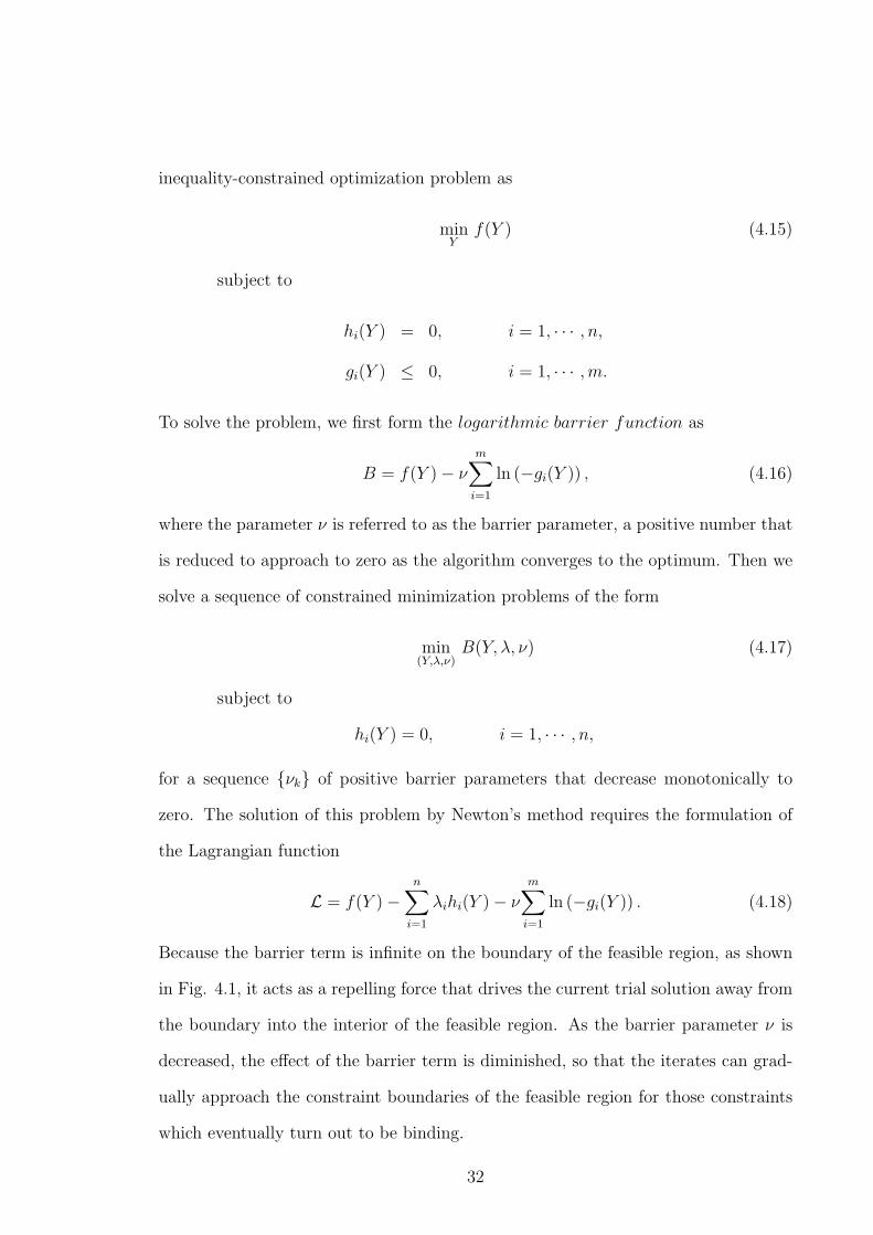
To solve the problem, we first form the logarithmic barrier function as
B = f(Y )− ν
m∑i=1
ln (−gi(Y )) , (4.16)
where the parameter ν is referred to as the barrier parameter, a positive number that
is reduced to approach to zero as the algorithm converges to the optimum. Then we
solve a sequence of constrained minimization problems of the form
min(Y,λ,ν)
B(Y, λ, ν) (4.17)
subject to
hi(Y ) = 0, i = 1, · · · , n,
for a sequence {νk} of positive barrier parameters that decrease monotonically to
zero. The solution of this problem by Newton’s method requires the formulation of
the Lagrangian function
L = f(Y )−n∑
i=1
λihi(Y )− ν
m∑i=1
ln (−gi(Y )) . (4.18)
Because the barrier term is infinite on the boundary of the feasible region, as shown
in Fig. 4.1, it acts as a repelling force that drives the current trial solution away from
the boundary into the interior of the feasible region. As the barrier parameter ν is
decreased, the effect of the barrier term is diminished, so that the iterates can grad-
ually approach the constraint boundaries of the feasible region for those constraints
which eventually turn out to be binding.
32
Figure 4.1: Effect of barrier term
To solve equation (4.17), we need to find the gradient of L with respect to Y :
∇YL = ∇Y f(Y )−n∑
i=1
λi∇Y hi(Y ) + ν
m∑i=1
1
−gi(Y )∇Y gi(Y )
= ∇Y f(Y )−n∑
i=1
λi∇Y hi(Y ) + ν
m∑i=1
1
si
∇Y gi(Y )
= ∇Y f(Y )−n∑
i=1
λi∇Y hi(Y ) +m∑
i=1
µi∇Y gi(Y )
= ∇Y f(Y )− hTY λ + gT
Y µ, (4.19)
where
−gi(Y ) = si, i = 1, · · · ,m,
µisi = ν, i = 1, · · · ,m,
hTY is a matrix consisting of the gradient ∇Y hi(Y ) as columns, and gT
Y is a matrix
consisting of the gradient ∇Y gi(Y ) as columns, or
hTY =
[∇Y h1(Y ) ∇Y h2(Y ) · · · ∇Y hn(Y )
],
gTY =
[∇Y g1(Y ) ∇Y g2(Y ) · · · ∇Y gm(Y )
].
Also, λ is a vector containing the elements λi, and µ is a vector containing the elements
33
µi. The set of equations we must solve is
∇Y f −n∑
i=1
λi∇hi +m∑
i=1
µi∇gi = 0, (4.20)
hi(Y ) = 0, i = 1, · · · , n (4.21)
gi(Y ) + si = 0, i = 1, · · · ,m (4.22)
µisi − ν = 0, i = 1, · · · ,m (4.23)
si > 0, i = 1, · · · ,m (4.24)
µi > 0, i = 1, · · · ,m (4.25)
These equations can be solved using the Newton iterative method. Our four sets
of variables for which we must solve are Y, λ, µ and s. The equation for a first order
approximation of a Taylor series of a function, F , whose independent variables are
Y, λ, µ and s is
F (Y, λ, µ, s) ∼= F (Yo, λo, µo, so) +∂F
∂Y4Y +
∂F
∂λ4λ +
∂F
∂µ4µ +
∂F
∂s4s. (4.26)
We want to find the values of Y, λ, µ and s where the expressions on the left side of
the equations we want to solve evaluate to zero. We use Newton-Raphson to do so.
Taking the first order approximation to the Taylor series for each of the four
expressions given in equations (4.20)-(4.23) and setting them equal to zero (the desired
value for each) give us
(∇Y f − hTY λ + gT
Y µ)
+ (∇2Y f −
n∑i=1
λi∇2Y hi +
m∑i=1
µi∇2Y gi)∆Y
−hTY ∆λ + gT
Y ∆µ = 0, (4.27)
h + hY ∆Y = 0, (4.28)
(g + s) + gY ∆Y + I∆s = 0, (4.29)
(MSe− νe) + S∆µ + M∆s = 0, (4.30)
34

where
I : an identity matrix,
S : a diagonal matrix constructed from (s1, s2, · · · , sm),
M : a diagonal matrix constructed from (µ1, µ2, · · · , µm),
e : a column vector with all elements 1.
The above equations can be organized in matrix form as
HY hTY gT
Y 0
hY 0 0 0
gY 0 0 I
0 0 S M
∆Y
∆λ
∆µ
∆s
=
−∇Y f + hTY λ− gT
Y µ
−h
−g − s
νe−MSe
, (4.31)
or
W∆z = ∆F, (4.32)
where
HY = ∇2Y f −
n∑i=1
λi∇2Y hi +
m∑i=1
µi∇2Y gi.
We initially set ν to some relatively large number, such as 10. Starting with an initial
guess
zo =
Yo
λo
µo
so
,
we calculate the W matrix and the ∆F vector. If all the elements of ∆F are suffi-
ciently close to zero, we have found the solution zo. Otherwise we must solve for ∆z
by
∆z = W−1∆F. (4.33)
35

Then the original z is updated by
z = zo + α∆z. (4.34)
However, following conditions need to be satisfied when updating z:
µi > 0,
si > 0.
Therefore, when calculating the updated µ and s, we must make sure that each µi
and each si is still strictly greater than zero when ∆µi and ∆si are added to it,
respectively. If adding ∆µi or ∆si violates this condition, all ∆µi and all ∆si must
be scaled by some factor α less than one before adding them as in (4.34).
Now that we have a new guess for z, the W matrix and ∆F vector are calculated
again. If the elements of the ∆F vector are sufficiently close to zero, we have found
the z which solves our problem. Otherwise we solve for ∆z and update z again. This
process is repeated until we find the z which makes ∆F very close to zero.
After we solve for z, we reduce the barrier parameter ν by some factor κ. For
example, if κ = 0.4, the barrier parameter ν is updated by letting the new ν be 0.4
times the old ν. Using the value of z obtained using the old ν as an initial guess
zo, we use the iterative procedure described above to solve for the value of z which
makes ∆F approximately zero for the new barrier parameter. The process of solving
for z, decreasing ν, and then solving for z again is repeated until ν becomes a very
small number, such as 10−10. This process is illustrated in Figure 4.2. When ν gets
this small, we have found the z that solves our problem. When solving for z given
a particular ν, it is not necessary to force ∆F to be zero. What we really want
to know is how close we are to the central path. The central path is defined by a
sequence of solutions {Y (ν), λ(ν), µ(ν), s(ν)} which make ∆F evaluate to zero for
every possible value of ν. One way of measuring how close we are to the central path
is by checking to see how close each product µisi is to the barrier parameter ν. One
36

Figure 4.2: Graphical representation of central path
proposed way of doing this is by first calculating the average value of µisi, also known
as the dualityfactor [13], by
ν =m∑
i=1
µisi
m, (4.35)
which evaluates to zero when each product µisi is equal to ν. Instead of checking to
see if ∆F is sufficiently close to zero, we check to see when the following is true:
∥∥∥∥∥∥∥∥∥∥∥∥∥
µ1s1 − ν
µ2s2 − ν
...
µmsm − ν
∥∥∥∥∥∥∥∥∥∥∥∥∥2
≤ τν (4.36)
where
0 < τ < 1.
When this logical statement becomes true, we are sufficiently close to the central
path, and we can reduce ν.
Despite several attractive features of the PDIP method, it has an inherent disad-
vantage that the size of problem is much bigger than the Newton active set method
since the PDIP method includes all inequality constraints. This problem becomes
37

even more involved when we consider a large scale natural gas and power system
network.
38

CHAPTER 5
NATURAL GAS FLOW MODELING
Natural gas is transported from gas producers to customers at various locations. A
typical natural gas transmission system today consists of a large number of gas pro-
ducers, various customers, storage, many compressor stations, thousands of pipelines,
and many other devices such as valves and regulators, including midstream gas pro-
cessing (between well and pipeline)
A typical pipeline network for transporting natural gas consumes a significant
amount of fuel per day to operate compressors pumping natural gas. This is because
there is a gas pressure loss due to friction between gas and pipe inner walls. Moreover,
energy is lost by heat transfer between gas and its environment. To compensate for
these losses of energy and to keep the gas flowing, compressor stations are installed
in the network, which consume a part of the transported gas resulting in economic
losses1.
The purpose of this chapter is to provide the underlying mathematical modeling
of natural gas transmission networks. It will include gas flow equations, compressor
horsepower equation, and matrix representations of natural gas networks.
1Losses often refer to leakage of natural gas from the pipeline system, which is negligible if there isno theft problem. We will use the term “losses” only for the gas required to power the compressors.
39

Figure 5.1: Pipeline network representation
5.1 Elements of Natural Gas Transmission Net-
work
Three basic types of entities are considered for the modeling of a natural gas trans-
mission network: pipelines, compressor stations, both of which are represented by
branches, and interconnection points, represented by nodes.
For simulation of a network, we assume that nodes represent pipeline connections
while branches represent pipelines and compressor stations, which have flow directions
assigned. We also have different types of nodes. A source node represents a gas
production or storage facility. A load node represents a place where gas is to be
taken out of the system, either for consumption or storage.
Each compressor branch defines two more node types technically referred to as
suction and discharge nodes. Likewise, each pipeline branch has two types of nodes, a
sending end node and a receiving end node. We define fkij (or fk for simple notation)
as the flow rate through a branch, say number k, which begins at node i and ends at
node j.
Figure 5.1 shows an example of a natural gas network. It is a simple tree-structure
pipeline network, which consists of one source at node 1, two loads at nodes T +
1 & K + 1, and several pipeline and compressor branches. wS1 is the amount of gas
supplied at the source node, and wLT+1& wLk+1
are the amounts of gas consumed at
the load nodes, respectively.
40
For a given gas network, there are three types of relevant decision variables: the
flow rate through a pipeline, the flow rate through a compressor, and the pressure
at each node. For a compressor, these variables are further restricted by a set of
constraints that depend on the operating attributes of the compressor.
5.2 Network Topology
Analysis of natural gas pipeline networks is relatively complex, particularly if the
network consists of a large number of pipelines, several compressors, and various sup-
pliers and consumers [21]. Matrix notation is a simple and useful way of representing
a network. In gas network analysis, matrices turn out to be the natural way of ex-
pressing the problem [22]. A gas pipeline system can be described by a set of matrices
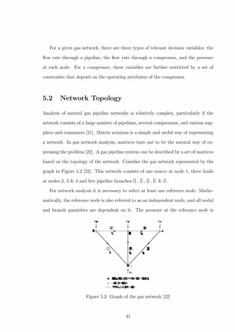
based on the topology of the network. Consider the gas network represented by the
graph in Figure 5.2 [22]. This network consists of one source at node 1, three loads
at nodes 2, 3 & 4 and five pipeline branches ①, ②, ③, ④ & ⑤.
For network analysis it is necessary to select at least one reference node. Mathe-
matically, the reference node is also referred to as an independent node, and all nodal
and branch quantities are dependent on it. The pressure at the reference node is
Figure 5.2: Graph of the gas network [22]
41
known. A network may contain several pressure-defined nodes and these form a set
of reference nodes for the network.
A gas injection node is a point where gas is injected into the network, which may
be positive, negative, or zero. Negative injection represents a load demand for gas
from the network. This node may be supplying domestic or commercial consumers,
charging gas storages, or even accounting for leakage in the network. A positive
injection represents a supply of gas to the network. It may take gas from storage,
source or another network. A zero injection is assigned to nodes that do not have a
load or source but are used to represent a point of change in the network topology,
such as a junction of several branches. Then, the vector of gas injections w at each
node for Figure 5.2 is defined as
w =
[w1 w2 w3 w4
]T
,
=
[wS1 −wL2 −wL3 −wL4
]T
,
where
wi = wSi− wLi
,
wSi= gas injection at node i,
wLi= gas removed at node i.
At steady-state conditions, the total load on the network is balanced by the supply
into the network at the source node.
To define the network topology completely, it is necessary to assign a direction to
each branch. Each branch direction is assigned arbitrarily and is assumed to be the
positive direction of flow in the branch. If the flow has a negative value, then the
direction of flow is opposite to the branch direction. References such as Osiadacz’s
book [22] may be consulted for further detail.
42

5.3 Matrix Representations of Network
The interconnection of a network can be described by the branch-nodal incidence
matrix A. This matrix is rectangular, with the number of rows NN equal to the
number of nodes (including reference nodes), and the number of columns NP equal
to the number of pipeline and compressor branches in the network. The element Aij
of the matrix A corresponds to node i and branch j, and is defined as
Aij =
+1, if pipeline branch j enters node i,
−1, if pipeline branch j leaves node i,
0, if pipeline branch j is not connected to node i.
For the network in Figure 5.2, the branch-nodal incidence matrix is
A =
−1 −1 −1 0 0
1 0 0 1 0
0 1 0 −1 −1
0 0 1 0 1
,
where NN = 4 nodes and NP = 5 branches. One important thing to note is that the
sum of all rows in the matrix A becomes zero due to the definition of each element
of the matrix A. Thus, the matrix A is always rank-1 deficient, and therefore the
matrix AAT is singular. This problem can be avoided by removing the rows of the
matrix A corresponding to known-pressure nodes, which will be discussed in next
chapter.
5.4 Flow Equation
For isothermal gas flow in a long horizontal pipeline, say number k, which begins at
node i and ends at node j, the general steady-state flow rate (in standard ft3/hr,
or SCF/hr at T0 = 520oR and P0 = 14.65 psia) is often expressed by the following
43

formula [22, 23] derived from energy balance:
fkij = Sij × 3.22T0
π0
√Sij
(π2
i − π2j
)D5
k
FkGLkTkaZa
, (5.1)
where
fkij = pipeline flowrate (SCF/hr),
Sij =
+1 if πi − πj > 0,
−1 if πi − πj < 0,
Fk = pipeline friction factor,
Dk = internal diameter of pipe between nodes (inch),
G = gas specific gravity (air=1.0, gas=0.6),
Lk = pipeline length between nodes (miles),
πi = pressure at node i (psia),
πj = pressure at node j (psia),
π0 = standard pressure (psia),
T0 = standard temperature (◦R),
Tka = average gas temperature (◦R),
Za = average gas compressibility factor.
There are several different flow equations in use in the natural gas transmission indus-
try [22, 24]. The differences are mainly due to the empirical expression assumed for
the friction factor, Fk, and in some cases the rigorous consideration of the deviation
of the behavior of natural gas from that of an ideal gas. The change of flow changing
from partial turbulence to full turbulence is referred as the transition region. The
Reynolds number, a measure of the ratio of the inertia force on an element of fluid to
the viscous force on an element, at which this transition occurs is dependent on the
diameter of the pipeline and its roughness, and is typically about 107 [22]. The extent
of the transition region is dependent on the system considered, and within this region
44
the frictional resistance depends on both the Reynolds number and the pipe charac-
teristics. However, in the fully-turbulent flow region for high-pressure networks, the
friction factor Fk is strictly dependent on pipeline diameter [22], [25]. That is
Fk =0.032
D1/3k
. (5.2)
Then, equation (5.1) becomes
fk = fkij = Sij Mk
√Sij
(π2
i − π2j
), SCF/hr (5.3)
where
Mk = ε18.062 T0 D
8/3k
π0
√GLkTkaZa
,
ε = pipeline efficiency.
As indicated in equation (5.3), gas flow can be determined once πi and πj are known
for given conditions. Equation (5.3), known as Weymouth flow equation, is most
satisfactory for large diameter (≥ 10 inches) lines with high pressures [23].
5.5 Compressor Horsepower Equation
During transportation of gas in pipelines, gas flow loses a part of its initial energy
due to frictional resistance which results in a loss of pressure. To compensate the loss
of energy and to move the gas, compressor stations are installed in the network. In
general, the nature of the compressor work function is very complex and depends also
on consideration such as the number of compressors running within the compressor
station, how the compressor units are configured (i.e. in series, in parallel, combina-
tion of both, etc.), physical properties of the compressor units, and type of compressor
unit [22]. One of the most common configurations implemented in practice is that
of compressor stations consisting of identical centrifugal compressor units operating
in parallel. Centrifugal compressors are versatile, compact, and generally used in the
45
range of 1,000 to 100,000 inlet ft3/min for process and pipeline compression applica-
tions [24]. In a centrifugal compressor, work is done on the gas by an impeller. Gas
is discharged at a high velocity into a diffuser. The velocity of gas is reduced and its
kinetic energy is converted to static pressure.
A key characteristic of the centrifugal compressor is the horsepower consumption,
which is a function of the amount of gas that flows through the compressor and the
relative boost ratio between the suction and the discharge pressures.
After empirical modification to account for deviation from ideal gas behavior, the
actual adiabatic (zero heat transfer) compressor horsepower equation [23] at To =
60oF (= 520oR) and πo = 14.65 psia becomes
Hk = Hkij = Bk fk
[(πj
πi
)Zki(α−1α )
− 1
], HP (5.4)
where
Bk =3554.58 Tki
ηk
(α
α− 1
),
fk = flow rate through compressor (SCF/hr),
πi = compressor suction pressure (psia),
πj = compressor discharge pressure (psia),
Zki = gas compressibility factor at compressor inlet,
Tki = compressor suction temperature (◦R),
α = specific heat ratio (cp/cV ),
ηk = compressor efficiency.
5.6 Conservation of Mass Flow
The mass-flow balance equation at each node can be written in matrix form as
(A + U)f + w −Tτ = 0, (5.5)
46
where
A = a branch-nodal incidence matrix,
Uik =
+1, if the kth unit has its outlet at node i,
−1, if the kth unit has its inlet at node i,
0, otherwise.
Tik =
+1, if the kth turbine gets gas from node i,
0, otherwise.
f = a vector of mass flow rates through branches,
w = a vector of gas injections at each node.
In addition to the matrix A, which represents the interconnection of pipelines and
nodes, we define the matrix U, which describes the connection of units (compressors)
and nodes. The vector of gas injections w is obtained by
w = wS − wL, (5.6)
where
wS = a vector of gas supplies at each node,
wL = a vector of gas demands at each node.
Thus, a negative gas injection means that gas is taken out of the network.
The matrix T and the vector τ represent where gas is withdrawn to power a gas
turbine to operate the compressor. So if a gas compressor, say k, between nodes i and
j, is driven by a gas-fired turbine, and the gas is tapped from the suction pipeline i,
we have the following representation:
Tik = +1, Tjk = 0 , and τk = amount tapped.
Conversely, if the gas were tapped at the compressor outlet, we would have
Tik = 0 , Tjk = +1, and τk = amount tapped.
47

Analytically, we will assume that τk can be approximated as
τk = αTk + βTkHkij + γTkH2kij, (5.7)
where Hk = Hkij is the horsepower required for the gas compressor k in equation
(5.4).
48
CHAPTER 6
NATURAL GAS LOADFLOW
The problem of simulation of a gas network with NN nodes in steady state, known
as loadflow , is usually that of computing the values of node pressures and flow rates
in the individual branches for known values of NS source pressures (NS ≥ 1) and of
gas injections in all other nodes.
Gas loadflow analyses are required operationally whenever significant changes in
demands or supplies are expected to occur. It is also used for system planning pur-
poses. For example, when a gas-fired generator is located in the gas network, we need
to see whether the network has enough capability to carry the required amount of gas
to the generator while satisfying various network constraints, such as pressure limits
at each node and compressor operation limits.
In this chapter, we state the loadflow problem in a general way, and construct
a mathematical formation. We present a loadflow problem for a network without
compressors. Then we introduce a general loadflow analysis with compressors. We
formulate the gas loadflow problem in a way similar to the electric loadflow problem,
and include the gas consumption rates at compressor stations.
However, we omit gas storage to avoid inter - temporal linkages-we only attempt
to solve the gas loadflow at a single time-a “snapshot”.
49

6.1 Loadflow Problem Statement
The gas loadflow problem is stated below:
• Given a natural gas system described by a branch-nodal incidence matrix A,
a unit-nodal incidence matrix U, a gas turbine-nodal incidence matrix T, and
given a set of gas injections except at the NS known-pressure sources (injections
at these nodes initially unknown), and each unit’s operating condition (such as
the compression ratio, the flow rate through the compressor, or the suction or
discharge pressure),
• determine all other pressures, and calculate the flow rates in all branches and
the gas consumptions at compressor stations.
Simply speaking, one of two quantities, nodal pressure πi and gas injection wi at each
node, and one compressor operating condition are specified, and other values are to
be determined. Specified quantities are chosen based on the following conditions:
Nodes:
• Known-Injection Node: For a node i of this type, we assume that we know
a gas injection wi, and the pressure πi is to be determined. Generally, source
and load nodes, and junctions with no gas injections belong to this node. Elec-
trically, this is analogous to a “load bus.”
In fact, solving the loadflow problem with only this type of node is not in general
possible. The first reason is that, in the flow equation (5.1), the pressures never
appear by themselves, but instead appear only as a squared-pressure difference of the
form π2i − π2
j . Therefore, there are only NN − 1 pressures which affect the loadflow.
We therefore pick NS ≥ 1 nodes to provide reference pressures. These nodes are
generally the external gas sources supplying our system.
50

Another reason is that with is that solving a loadflow for a network containing only
known-injection nodes would imply that we know the gas injections at every single
node. In fact, we cannot mathematically specify all NN gas injections, as it may
not be possible to find a solution to the loadflow equations. Specifying the injections
at all nodes is the same as specifying the gas supplies to gas turbines driving gas
compressors, which we cannot know until the loadflow is solved. Instead, we must
pick at least one node, allowing the set of gas injection(s) to be whatever is required
to solve the loadflow equations. Thus, we have to specify another node type:
• Known-Pressure Node: Each is typically one of the source nodes, and the
pressures of such nodes serve as references for all other pressures. We assume
that we know {πi, i = 1, . . . , NS}, but we do not know the corresponding gas
injections. Electrically this is analogous to a (possibly distributed) “slack bus.”
In addition to nodes, the other main components are branches, which connect
the nodes.
Branches:
• Pipelines: Pipeline flow modelling has already been discussed in the previous
chapter. Other than the physical characteristics of the pipeline, the only vari-
ables that the flow fk = fkij on pipeline k depends on are the pressures πi and
πj at the two ends of the pipeline.
• Compressors: The other key component we will model in a gas network is a
compressor (also called a unit). The connection between the unit’s inlet and
outlet nodes is not defined by the branch-nodal incidence matrix A, but by U.
The compression ratio between the compressor inlet and outlet, and the flow
rate through the compressor are governed by the horsepower equation (5.4), not
by the flow equation (5.1). Compressor data (other than the physical charac-
teristics of the compressor) can be specified in several ways [22] for compressor
51

k: relative boost Rk = Rkij = πj/πi, or absolute boost πj − πi, or mass-flow
rate fkij. The inlet pressure πi or the outlet pressure πj could also be specified.
6.2 Loadflow without Compressors
We will first consider a gas network with only pipelines to explain the Newton-nodal
method. Assume that node 1 is the known-pressure node, and all other nodes are
the known-injection nodes. Since we do not have compressors, the unit’s inlet-outlet
nodes are not defined. Then the loadflow problem is described as follows:
Given : π1 w2 . . . wNN
Determine : w1 π2 . . . πNN
It appears that we have NN − 1 quantities known, and NN − 1 quantities unknown.
The set of nodal flow equations that describes a gas network with only pipelines is
given by
w = A1 · f(π, π), (6.1)
where
A1 = a branch-nodal incidence matrix except the known-pressure nodes,
w = ws − wL,
f = a vector of flow rates through pipelines.
We used π to indicate the part of π we know, and π for unknown part. Likewise for
w. Flow equation (5.3) is used to get each pipeline branch flow as
fkij = Sij Mk
√Sij
(π2
i − π2j
), SCF/hr (6.2)
In the Newton-nodal method [22], an initial approximation is made to the nodal
pressures. This approximation is then iteratively corrected until the final solution is
52
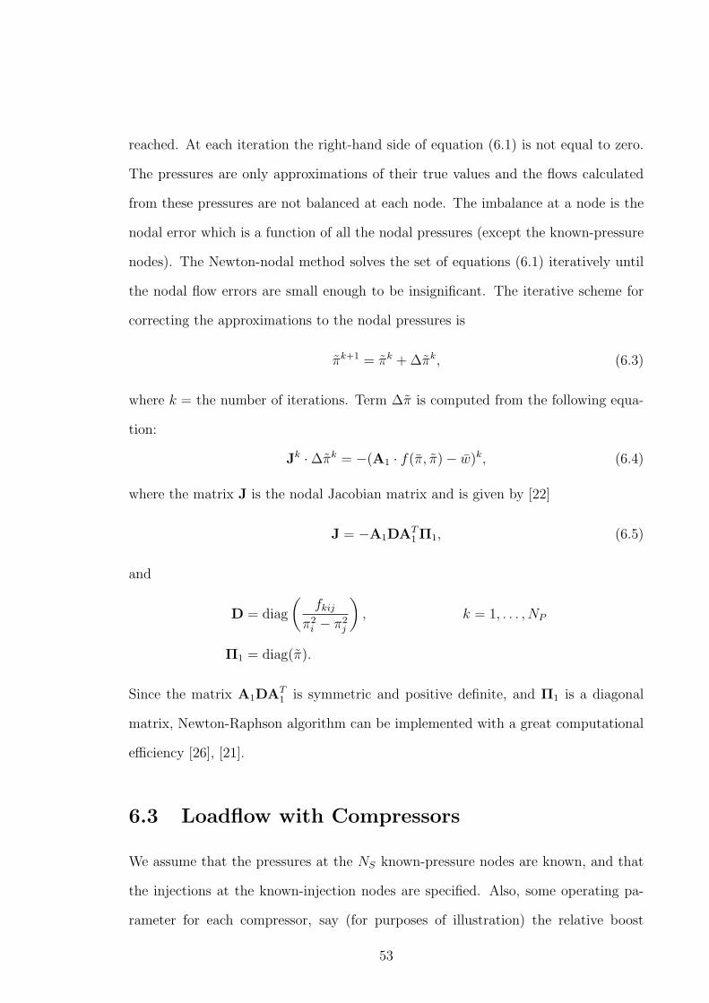
reached. At each iteration the right-hand side of equation (6.1) is not equal to zero.
The pressures are only approximations of their true values and the flows calculated
from these pressures are not balanced at each node. The imbalance at a node is the
nodal error which is a function of all the nodal pressures (except the known-pressure
nodes). The Newton-nodal method solves the set of equations (6.1) iteratively until
the nodal flow errors are small enough to be insignificant. The iterative scheme for
correcting the approximations to the nodal pressures is
πk+1 = πk + ∆πk, (6.3)
where k = the number of iterations. Term ∆π is computed from the following equa-
tion:
Jk ·∆πk = −(A1 · f(π, π)− w)k, (6.4)
where the matrix J is the nodal Jacobian matrix and is given by [22]
J = −A1DAT1 Π1, (6.5)
and
D = diag
(fkij
π2i − π2
j
), k = 1, . . . , NP
Π1 = diag(π).
Since the matrix A1DAT1 is symmetric and positive definite, and Π1 is a diagonal
matrix, Newton-Raphson algorithm can be implemented with a great computational
efficiency [26], [21].
6.3 Loadflow with Compressors
We assume that the pressures at the NS known-pressure nodes are known, and that
the injections at the known-injection nodes are specified. Also, some operating pa-
rameter for each compressor, say (for purposes of illustration) the relative boost
53

Rk = Rkij, is specified, and let’s say there are NP branches in the system, of which
NC are compressors. We can state the loadflow problem this way:
Given :
π1 · · ·πNSwNS+1. . .wNN
R1· · ·RNC
Find :
w1 · · ·wNSπNS+1 . . .πNN
f1 · · ·fNCfNC+1. . .fNP
It appears that there are NN +NC quantities given, while NN +NP must be found.
It is clear that
NC < NP .
This inequality is strict, unless we have no pipelines at all, only NP compressors
connected to each other without any intervening pipelines – a silly situation. So since
NN + NC < NN + NP , the system appears to be undetermined. Note, however,
that from (6.2), the flow fk depends only on the pressures πi and πj of the nodes it
connects. Likewise, the horsepower Hk required by the compressor depends only on
the flow fk and the ratio Rk = πj/πi, and therefore only depends on the pressures πi
and πj. The tap-off loss τk depends only on Hk and thus on the nodal pressures. So, if
we knew {πi, i = 1, . . . , NN}, we would know all other quantities we have discussed.
But we only know them for i = 1, . . . , NS. Let’s use π to indicate the part of π we
know, and π for the unknown part. Likewise for w and w. The objective, then, is
to calculate π, giving us the entire vector π, from which all other quantities can be
calculated.
We can use the mass-balance equation (5.5) to write
w = Tτ(π, π)− (A + U)f(π, π),
where A, U, and T are obtained from A, U, and T as in equation (5.5) after we
have removed the rows corresponding to the NS nodes (the known-pressure nodes
with unknown injections), that is, we have dropped the first NS equations of (5.5)
54

corresponding to w. This gives us NN − NS equations (for the elements of w) in
NN −NS unknowns (the elements of π). At this point, standard Newton-Raphson or
other iterative methods can be employed to drive the “mismatch” ∆w (the difference
between the values of w computed from above and the true values of w given as part
of the data) to zero by correcting our current guess for the correct value of π.
We have shown that the dimension of the load flow problem with compressors is
NN −NS. However, it is convenient to add new equations and new variables if they
make the problem easier to implement. Since the compressor horsepower in equation
(5.4) and the gas consumption rate in equation (5.7) are functions of horsepowers,
compressor flow rates, and gas consumption rates as well as the specified relative
boost rates, we will add three extra decision variables for each compressor station.
Then the new decision variables become
x =
[πT HT τT fT
C
]T
,
where
H = a vector of horsepowers at each compressor,
τ = a vector of gas consumptions at each compressor,
fC = a vector of compressor branch flow rates.
Since there are NN − NS + 3NC decision variables, we need to define extra 3NC
equations. The mass-flow balance equations F1 in matrix form are given by
F1 = (A + U) ·
fC
fP (π, π)
+ w − T · τ = 0, (6.6)
where fP (π, π) is a vector of mass flow rates through pipelines, which are obtained by
flow equation (6.2). Note that the size of the vector F1 is NN −NS. Assuming that
the compression ratio Rkijis given, and gas compressor k located between nodes i and
j is driven by a gas-fired turbine, the extra 3NC equations related with compressor
55

operation are
F2k= τk − αTk − βTkHkij − γTkH
2kij = 0, k = 1, . . . , NC (6.7)
F3k= Hkij −Bk fCk
[(πj
πi
)Zki(α−1α )
− 1
]= 0, k = 1, . . . , NC (6.8)
F4k=
(πj
πi
)−Rkij
= 0, k = 1, . . . , NC (6.9)
Let us define the vector of error functions F(x) by
F(x) =
F1(x)
F2(x)
F3(x)
F4(x)
.
Note that there are NN −NS +3NC equations and NN −NS +3NC unknown decision
variables. So we have the right number of variables to force all the mismatches to zero
by using Newton-Raphson or other iterative methods. The iteration will be repeated
until the mismatches become small enough to be insignificant.
56

CHAPTER 7
UPFC MODELING FOR STEADY-STATE ANALYSIS
Modeling UPFC for steady-state analysis has been considered by several researchers
and an injection model [6] and an uncoupled model [14] have been proposed. These
models can be easily incorporated into steady-state loadflow or optimal power flow
studies. However, these models employ four UPFC control variables that depend on
the UPFC input and output currents and voltages and both models require adding
two additional buses to the loadflow or OPF problem formulation. The voltage and
current relationships between UPFC input and output need to be included explicitly.
In addition, a constraint on real power conservation needs to be added, thereby
reducing the degrees of freedom four to three. Since electricity prices at the UPFC
input and output buses, which are the dual variables (or “shadow” prices) associated
with real and reactive power injections, are meaningless when no power is bought or
sold at these fictitious buses, their addition to the problem only serves to increase the
size of the problem. Therefore, these models are undesirable for our UPFC sensitivity
analysis.
To overcome these problems, a new steady-state mathematical model for a UPFC,
the UPFC ideal transformer model, is proposed. In this model, UPFC control vari-
ables do not depend on UPFC input and output voltages and currents, and therefore
addition of fictitious input and output buses are not necessary. This model is eas-
ily combined with transmission line models using ABCD two-port representations,
57
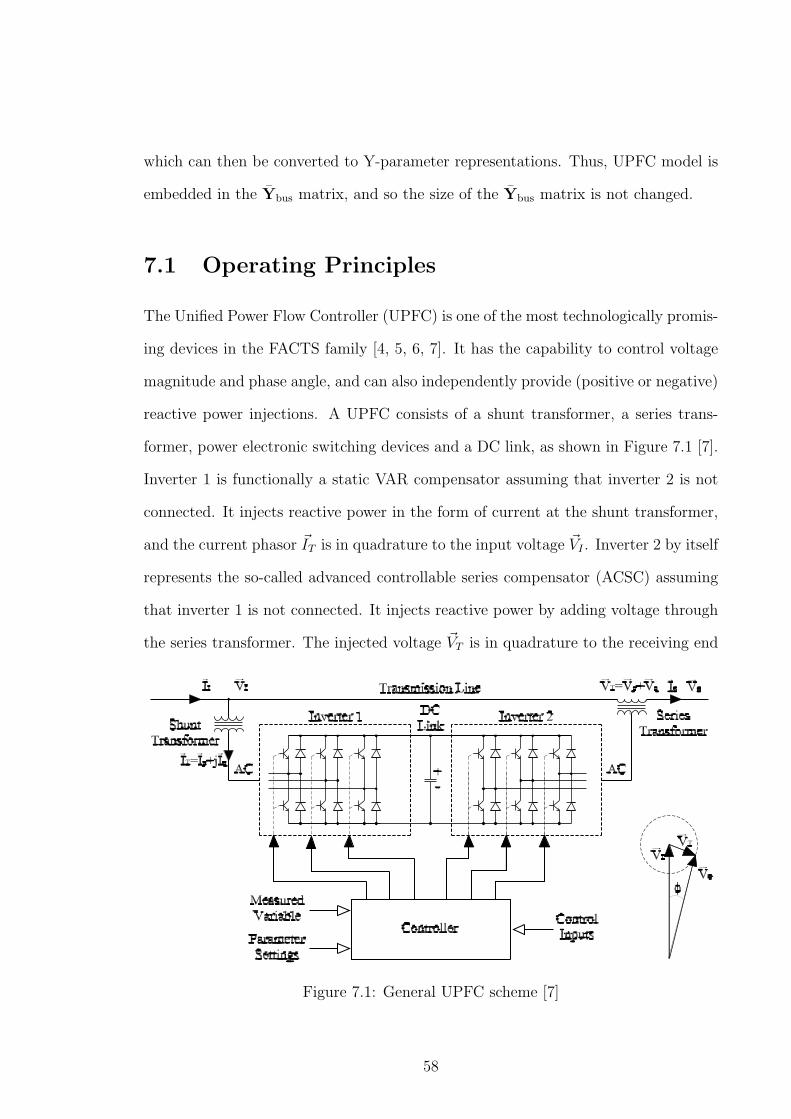
which can then be converted to Y-parameter representations. Thus, UPFC model is
embedded in the Ybus matrix, and so the size of the Ybus matrix is not changed.
7.1 Operating Principles
The Unified Power Flow Controller (UPFC) is one of the most technologically promis-
ing devices in the FACTS family [4, 5, 6, 7]. It has the capability to control voltage
magnitude and phase angle, and can also independently provide (positive or negative)
reactive power injections. A UPFC consists of a shunt transformer, a series trans-
former, power electronic switching devices and a DC link, as shown in Figure 7.1 [7].
Inverter 1 is functionally a static VAR compensator assuming that inverter 2 is not
connected. It injects reactive power in the form of current at the shunt transformer,
and the current phasor ~IT is in quadrature to the input voltage ~VI . Inverter 2 by itself
represents the so-called advanced controllable series compensator (ACSC) assuming
that inverter 1 is not connected. It injects reactive power by adding voltage through
the series transformer. The injected voltage ~VT is in quadrature to the receiving end
Figure 7.1: General UPFC scheme [7]
58
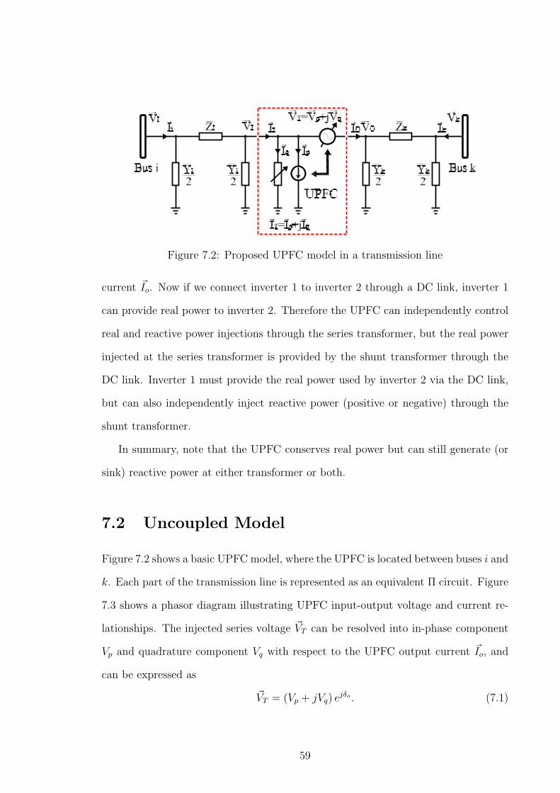
Figure 7.2: Proposed UPFC model in a transmission line
current ~Io. Now if we connect inverter 1 to inverter 2 through a DC link, inverter 1
can provide real power to inverter 2. Therefore the UPFC can independently control
real and reactive power injections through the series transformer, but the real power
injected at the series transformer is provided by the shunt transformer through the
DC link. Inverter 1 must provide the real power used by inverter 2 via the DC link,
but can also independently inject reactive power (positive or negative) through the
shunt transformer.
In summary, note that the UPFC conserves real power but can still generate (or
sink) reactive power at either transformer or both.
7.2 Uncoupled Model
Figure 7.2 shows a basic UPFC model, where the UPFC is located between buses i and
k. Each part of the transmission line is represented as an equivalent Π circuit. Figure
7.3 shows a phasor diagram illustrating UPFC input-output voltage and current re-
lationships. The injected series voltage ~VT can be resolved into in-phase component
Vp and quadrature component Vq with respect to the UPFC output current ~Io, and
can be expressed as
~VT = (Vp + jVq) ejδo . (7.1)
59

Figure 7.3: Phasor diagram of UPFC input-output voltages and currents
Since ~VT is dependent on the UPFC output current phase angle δo, it requires adding
an extra bus for the UPFC output terminal. The current IT injected by the shunt
transformer contains a real component Ip, which is in phase or in opposite phase with
the input voltage. It also has a reactive component Iq, which is in quadrature with
the input voltage. Then the injected current ~IT can be written by
~IT = (Ip + jIq) ejθI , (7.2)
where θI is the UPFC input voltage phase angle. Thus, a second extra bus is required
for the UPFC input terminal.
The UPFC input-output voltage and current can be represented by
~Vo = ~VI + ~VT = VIejθI + Vpe
jδo + jVqejδo , (7.3)
~Io = ~II − ~IT = IIejδI − Ipe
jθI − jIqejθI , (7.4)
where δI is the UPFC input current phase angle. Then, the complex power injected
into the transmission line by the series transformer can be resolved into the real and
reactive power in simple form as
ST = ~VT · ~I∗o = Vp · Io︸ ︷︷ ︸PT
+ jVq · Io︸ ︷︷ ︸QT
. (7.5)
60

Figure 7.4: Uncoupled UPFC model in a transmission line.
The in-phase voltage Vp is associated with a real power supply and the quadrature
voltage Vq with an inductive or capacitive reactance in series with the transmission
line.
Since the real power PT (which may be negative) is provided by the current Ip in
the shunt transformer, we can derive the following relationship:
Vp · Io − VI · Ip = 0. (7.6)
or the real power input equals the real power output. Due to (7.6), the number of
degrees of freedom for the UPFC is reduced to three.
Now that two extra buses for the UPFC input and output terminals are added, and
the UPFC voltage and current relationships (7.3, 7.4) and real power flow equation
(7.6) are established, we can represent the UPFC uncoupled model as shown in Figure
7.4. The currents injected into the UPFC input and output buses are
~II =
(Yi
2+
1
Zi
)~VI − 1
Zi
~Vi , (7.7)
~Io =
(Yk
2+
1
Zk
)~Vo − 1
Zk
~Vk . (7.8)
The magnitudes of the injected voltage VT and current IT are limited by the maximum
voltage and current ratings of the inverters and their associated transformers, which
need to be included as inequality constraints in OPF.
61

7.3 Ideal Transformer Model
Since the UPFC conserves real power, and generates or consumes reactive power, it
can be modelled using an ideal transformer and a shunt branch, as shown in Figure
7.5 [27]. The advantage of this model is that the ideal transformer turns ratio and
the variable shunt susceptance are independent variables, which are not directly as-
sociated with the UPFC input-output voltages and currents. We define the UPFC
variables as follows:
T = transformer voltage magnitude turns ratio (real),
φ = phase shifting angle,
ρ = shunt susceptance,
and the ideal transformer turns ratio can be written by
T = Tejφ.
It is important to note that the ideal transformer does not generate real and reactive
power, and the reactive power is generated (or consumed) by the shunt admittance
only.
Since the UPFC input-output voltage and current relationship can be expressed
Figure 7.5: UPFC ideal transformer model
62

as
~VI = ~VoT∠φ, (7.9)
~II = jT ρ~Vo +1
T ∗~Io, (7.10)
the UPFC can be represented by an ABCD matrix as
~VI
~II
= ABCDU ·
~Vo
~Io
, (7.11)
where
ABCDU =
T 0
jT ρ 1T ∗
. (7.12)
Note that equation (7.11) is not bilateral unless T = 1∠0.
Now, we will show that this ideal transformer model represents the UPFC by
comparing the complex power injections at the UPFC input and output. Using (7.11),
the complex power injection at the UPFC input can be obtained by
SI = ~VI~I∗I , (7.13)
= T ~Vo
(jT ρ~Vo +
1
T ∗~Io
)∗,
= ~Vo~I∗o − j|T |2 · |~Vo|2ρ,
= So − j|T |2 · |~Vo|2ρ,
and the real and reactive power injections can be obtained by
PI = Real(SI
), QI = Imag
(SI
),
Po = Real(So
), Qo = Imag
(So
).
Thus, we can derive the following relationships between the UPFC input and output:
PI = Po, (7.14)
Qo = QI + |T |2 · |~Vo|2ρ. (7.15)
63
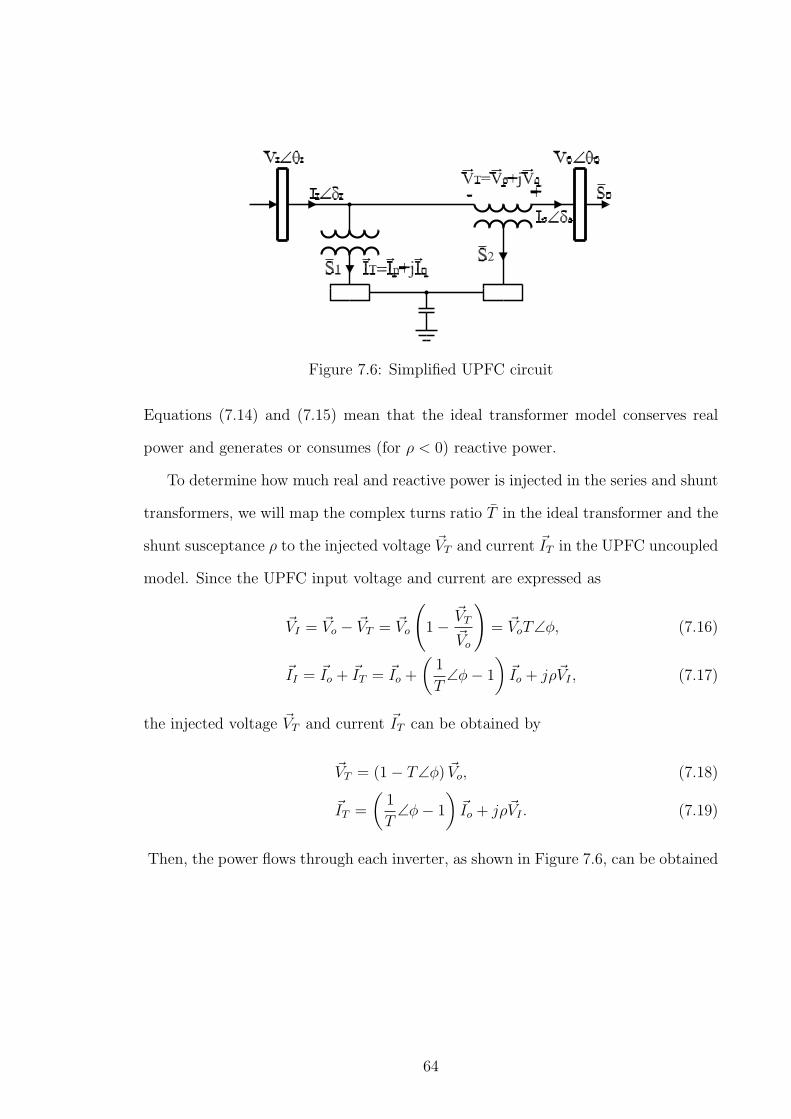
Figure 7.6: Simplified UPFC circuit
Equations (7.14) and (7.15) mean that the ideal transformer model conserves real
power and generates or consumes (for ρ < 0) reactive power.
To determine how much real and reactive power is injected in the series and shunt
transformers, we will map the complex turns ratio T in the ideal transformer and the
shunt susceptance ρ to the injected voltage ~VT and current ~IT in the UPFC uncoupled
model. Since the UPFC input voltage and current are expressed as
~VI = ~Vo − ~VT = ~Vo
(1−
~VT
~Vo
)= ~VoT∠φ, (7.16)
~II = ~Io + ~IT = ~Io +
(1
T∠φ− 1
)~Io + jρ~VI , (7.17)
the injected voltage ~VT and current ~IT can be obtained by
~VT = (1− T∠φ) ~Vo, (7.18)
~IT =
(1
T∠φ− 1
)~Io + jρ~VI . (7.19)
Then, the power flows through each inverter, as shown in Figure 7.6, can be obtained
64
by
S1 = ~VI~I∗T ,
= ~VoT∠φ
[(1
T∠φ− 1
)~Io + jρ~VoT∠φ
]∗,
= (1− T∠φ) So − jρ|T |2|~Vo|2, (7.20)
S2 = −~VT~I∗o ,
= (T∠φ− 1) ~Vo~I∗o ,
= (T∠φ− 1) So. (7.21)
Thus,
S1 + S2 = −jρ|T |2|~Vo|2, (7.22)
which verifies that the UPFC conserves real power and can generate (or consume)
reactive power.
Since the UPFC is modelled using passive circuit elements only, non-ideal UPFC
characteristics, such as shunt and series transformer reactances can be easily incor-
porated into this framework.
7.4 UPFC in a Transmission Line
A two-port ABCD matrix is the most convenient method to represent cascaded net-
works [9]. Let us divide a transmission line between buses i and k with a UPFC into
three cascaded networks, a UPFC input transmission line, a UPFC, and a UPFC
output transmission line, as shown in Figure 7.7. The UPFC input transmission line
, and the UPFC output transmission line are easily represented by two-port ABCD
matrices since the transmission lines are modelled using Π equivalent circuits. We call
ABCDi and ABCDk as the ABCD matrices for each transmission line, and defined
65
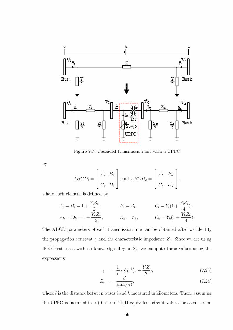
Figure 7.7: Cascaded transmission line with a UPFC
by
ABCDi =
Ai Bi
Ci Di
and ABCDk =
Ak Bk
Ck Dk
,
where each element is defined by
Ai = Di = 1 +YiZi
2, Bi = Zi, Ci = Yi(1 +
YiZi
4),
Ak = Dk = 1 +YkZk
2, Bk = Zk, Ck = Yk(1 +
YkZk
4).
The ABCD parameters of each transmission line can be obtained after we identify
the propagation constant γ and the characteristic impedance Zc. Since we are using
IEEE test cases with no knowledge of γ or Zc, we compute these values using the
expressions
γ =1
lcosh−1(1 +
Y Z
2), (7.23)
Zc =Z
sinh(γl), (7.24)
where l is the distance between buses i and k measured in kilometers. Then, assuming
the UPFC is installed in x (0 < x < 1), Π equivalent circuit values for each section
66
of the transmission line can be found by
Zi = Zc sinh(γl · x),
Yi =2
Zi
(cosh(γl · x)− 1) ,
Zk = Zc sinh(γl · (1− x)),
Yk =2
Zk
(cosh(γl · (1− x)− 1) .
Now, the three cascaded networks are combined to obtain
~Vi
~Ii
= ABCDi · ABCDU · ABCDk
~Vk
−~Ik
, (7.25)
=
Aik Bik
Cik Dik
~Vk
−~Ik
,
where ABCDU is given in (7.12). So
Aik = TAiAk + jTBiAkρ +1
T ∗BiCk,
Bik = TAiBk + jTBiBkρ +1
T ∗BiDk,
Cik = TCiAk + jTDiAkρ +1
T ∗DiCk,
Dik = TCiBk + jTDiBkρ +1
T ∗DiDk.
By rearranging (7.25) and solving for Ii and Ik, we have
~Ii
~Ik
= Ybusik
~Vi
~Vk
, (7.26)
where
Ybusik=
Dik
BikCik − AikDik
Bik
− 1Bik
Aik
Bik
.
In general,
det
Aik Bik
Cik Dik
= 1∠2φ, (7.27)
67

If φ = 0, that is, complex T is real, this determinant is one at angle zero, and complex
Ybusikbecomes symmetrical. Note that equation (7.25) represents a bilateral two port
network only if T = 1∠0.
As seen in (7.26), since the UPFC is embedded in the Ybus matrix, the size of the
Ybus matrix is not changed, so UPFC sensitivity analysis can be performed using this
ideal transformer model.
68

CHAPTER 8
GAS AND ELECTRICITY OPTIMAL POWER FLOW
The purpose of this chapter is to construct a mathematical formulation to solve
natural gas and electricity optimal power flow problems. To do this we present a
simple combined gas and electric network, and synthesize an optimal gas flow (OGF)
and an optimal electric power flow (OPF) into a single natural gas and electricity
optimal power flow (GEOPF) problem. Though this integration of gas and electric
system is based upon deterministic prices of gas in source nodes, we will certainly
need this GEOPF algorithm for stochastic cases for future studies where the price will
be a stochastic variable. For our purposes, gas and electricity storage are neglected.
8.1 Gas and Electric Combined Network
For an integrated gas and electric network, even though the gas network and electric
network are physically overlapped, we represent the two systems separately. One
example is shown in Figure 8.1. Electric generator buses which are coincident with
any gas nodes can be used to integrate the gas and electric networks. The generators
in the combined nodes are assumed to be driven by gas-powered turbines.
69

Figure 8.1: Combined natural gas and electricity network
8.2 Gas and Electricity Optimal Power Flow
The mathematical formulation of the GEOPF can be expressed as
minY
C(Y )−B(Y ) (8.1)
subject to:
hi(Y ) = 0, i = 1, . . . , n (8.2)
gj(Y ) ≤ 0, j = 1, . . . ,m (8.3)
where
• C(Y ) is total cost of system operation, and B(Y ) is the total benefit to society
and is treated as a negative cost. SW = B(Y )−C(Y ) is the social welfare, which
is the total benefit B(Y ) to society, less the cost of combined system operation,
and thus is the negative of the net cost of system operation to society. So
minimizing net cost C(Y )−B(Y ) is the same as maximizing social welfare.
70

• Y is a vector of decision variables (i.e. the voltage magnitude and angle at each
bus, real and reactive power generations, real and reactive power consumptions,
nodal pressures, flow rates through pipelines, flow rates through compressors,
gas consumptions by gas turbines, etc.).
• h is a set of equality constraints, such as the real and reactive power balance at
each bus, pipeline branch flow rates, the mass flow balance at each node, etc..
• g is a set of inequality constraints, such as line flow limits, voltage limits, gen-
eration limits, relative boost limits, nodal pressure limits, etc..
Then the Lagrangian for the GEOPF problem can be written
L(Y ) = −SW (Y )−n∑
i=1
λihi(Y ) +m∑
j=1
µjgj(Y ). (8.4)
Here, the objective of the GEOPF is to maximize the social welfare, while satisfying
n equality constraints and m inequality constraints.
8.2.1 Cost, Benefit, and Social Welfare
In the “Poolco” environment, central dispatch sets the price of gas or electricity in
the system to optimize a network-wide non-discriminatory service, while consumers
and producers contract competitively [8, 1]. The type of problem that the system
operator wishes to solve is an optimal power flow (OPF) problem in electricity and
an optimal gas flow (OGF) problem in natural gas, but doing so simultaneously in
an integrated manner.
The objective function to be maximized that we will use in the GEOPF problem
is social welfare [8]. To understand the concept of the social welfare, we introduce
the fact that there are two types of market participants, producers and consumers. A
producer is a supplier of some type of goods. Of course, there is a cost to produce the
good. Let’s say we know the cost of producing the good as a function of the amount
71

of the good that is produced. In our case, the electricity producer is supplying electric
power, so its cost is a function of the amount of real power PG it produces. The total
cost of real power generation is then (assuming quadratic cost curves)
CE =
NG∑i=1i/∈G
CEi(PGi
), (8.5)
=
NG∑i=1i/∈G
[αGi
+ βGiPGi
+ γGiP 2
Gi
],
where
NG = total number of real power generators,
αGi, βGi
, γGi= cost coefficients of real power generator i,
G = electric nodes with gas-fired generators.
For the combined node, it is important to note that the electric generation cost is not
included in the equation (8.5). This is because the combined nodes simply transform
gas energy into electric energy.
For the gas supplier, its production cost is a function of the amount of gas pro-
duced. Then, the total production cost becomes
CG =
NS∑i=1
ciwSi106 ×GHV, (8.6)
where
NS = total number of source nodes,
ci = gas production cost at source node i ($/MMBTU),
GHV = gas gross heating value (BTU/SCF).
A consumer purchases a good because he receives some benefit from using the
good. Let us say that this benefit that he/she receives can be measured in dollars
and is a quadratic function of the amount of the goods purchased. For the electric
72
power consumer, the benefit BE in dollars is a function of the amount of real power PL
consumed. The total benefit received from the consumption of real power (assuming
quadratic benefits) by loads is obtained by
BE =
NEL∑i=1
BEi(PLi
), (8.7)
=
NEL∑i=1
[βELi
PLi+ γELi
P 2Li
],
where
NEL = total number of electric consumers,
βELi, γELi
= benefit coefficients of real power consumer i.
For a gas consumer, his benefit BG is a function of the amount of gas consumed.
Then, the total benefit received from the consumption of gas is expressed as
BG =
NGL∑i=1i/∈G
BGi(wLi
), (8.8)
=
NGL∑i=1i/∈G
[βGLi
wLi+ γGLi
w2Li
],
where
NGL = total number of gas consumers,
βGLi, γGLi
= benefit coefficients of gas consumer i.
Note again that the gas consumer’s benefit at the combined node is not included since
this node is simply converting gas energy to electric energy.
Now we define the meaning of social welfare. It is the total benefit received by
society due to the production and consumption of the good. In the case of a combined
gas and electric network, the social welfare is defined as
SW = BE + BG − CE − CG (8.9)
=
NEL∑i=1
BEi(PLi
) +
NGL∑i=1i/∈G
BGi(wLi
)−NG∑i=1i/∈G
CEi(PGi
)−NS∑i=1
CGi(wsi
),
73

and it is the objective function of the GEOPF which we want to maximize, or the
negative of that which we wish to minimize.
8.2.2 Constraints
The GEOPF is a constrained optimization problem, which must satisfy various equal-
ity and inequality constraints at the optimum.
• Equality Constraints
– Electric Network
Kirchoff’s laws must be satisfied at each electric bus, resulting in the stan-
dard power flow (power balance) equations at each bus
PGi− PLi
= Pi(V, θ), i = 1, . . . , NB (8.10)
QGi−QLi
= Qi(V, θ), i = 1, . . . , NB (8.11)
The above two equations are conventional power flow equations, and tell
that the real and reactive power injection at each bus is a function of the
system bus voltage magnitudes and phase angles, or Pi(V, θ) and Qi(V, θ).
In our notation, V is the vector of system bus voltage magnitudes, and θ
is the vector of bus voltage phase angles. The amount of reactive power
consumed by the load, QL, is not considered a variable since it will be
assumed that the load has a fixed power factor where the power factor is
defined as
p.f. =PL√
P 2L + Q2
L
. (8.12)
This assumption is not critical to our formulation, and is made for simplic-
ity and concreteness only. Then QL is a linear function of the real power
74
consumed, or
QL(PL) =PL
p.f.
√1− p.f.2 . (8.13)
The real and reactive injection at bus i can be obtained by
Si(V, θ) = ~Vi~I∗i , i = 1, . . . , NB (8.14)
Pi(V, θ) = Re(Si),
Qi(V, θ) = Im(Si),
where the vector of current injections at each bus is obtained by
~I = Ybus · ~V .
– Gas Network
There are two sets of steady-state network flow equations, which must be
satisfied as equality constraints. The first equality constraint says that
the amount of gas at node i transported from and to other nodes must be
the same as that of gas injected at that node. This is known as a mass
flow balance equation. The set of mass flow equations that describe a gas
network is given by
(A + U)f + w −Tτ = 0, (8.15)
where units of f , w and τ are SCF/hr, hence equivalent to conversation
of mass. Note that the flow rates to the compressor inlet and from the
compressor outlet are different if the compressor is driven by a gas-fired
turbine. τk is the amount of gas supplied to gas-fired turbine k measured
in SCF/hr. For simplicity, we assume
τk = αTk + βTkHk + γTkH2
k , k = 1, . . . , NC (8.16)
where Hk is the horsepower required for compressor k, and defined by
Hk = Bk fk
[(πj
πi
)Zki(α−1α )
− 1
]. k = 1, . . . , NC (8.17)
75

The other equality constraint which is described by equation (5.3) is the
pipeline gas flow rate through each pipeline, and it is stated by
π2i − π2
j =1
M2k
Sij f 2kij, i, j = 1, . . . , NN (8.18)
Note that while the nodal flow equation (8.15) is linear, the pipeline branch
flow equation (8.18) is quadratic, and we need to take into account the fact
that the flow direction must be explicitly accounted for (by Sij.
– Gas and Electricity Combined Node
This is the location of an actual or planned gas-fired generation facility,
which would be located where a gas node and an electric power bus have a
common location. The gas node may have other loads or input injections,
as may the electrical node the generator is connected to. Let us suppose
that the electrical bus in question is i, which is fed gas from gas node ji.
Then
wji= wji,other (8.19)
− (aGi
+ bGiPGi
+ cGiP 2
Gi
) 1
GHV, i ∈ G
where
GHV = gas gross heating value (BTU/SCF),
aGi, bGi
, cGi= gas fuel rate coefficients at node i,
G = electric nodes with gas-fired generators.
• Inequality Constraints
– Electric Network
The system operating constraints include maximum and minimum limits
76
on the voltage magnitude at each bus and the magnitude of the line current
flowing on each line. These can be written as
Vmini≤ Vi ≤ Vmaxi
, i = 1, . . . , NB (8.20)
for the voltage magnitude at bus i, and
I2ikmax
≥∣∣∣~Iik
∣∣∣2
= ~Iik · ~I∗ik, i, k = 1, . . . , NB (8.21)
where
~Iik =(
~Vi − ~Vk
)yik + ~Viyshuntik
for the magnitude of the line current from bus i to bus k. Equation (8.21)
is called a transmission thermal limit. Since the voltage magnitude at
each bus is changed, we use the line current instead of the apparent power
flowing on each line for the thermal limit, although an apparent power
constraint could be used instead. Also, if voltage drop or the steady state
stability limits real power flow, these constraints could be used instead.
There are also limits on the amount of real and reactive power produced
by each generator. There may also be a limit on the amount of real power
consumed by each load. This gives us an additional set of inequality con-
straints.
PGmini≤ PGi
≤ PGmaxi, i ∈ NPG (8.22)
QGmini≤ QGi
≤ QGmaxi, i ∈ NQG (8.23)
PLmini≤ PLi
≤ PLmaxi, i ∈ NEL (8.24)
The tap magnitude and the tap angle of a regulating transformer, the volt-
age magnitude and the angle drop along a transmission line, MW inter-
change transactions, shunt reactors or capacitors, etc. can be also included
as inequality constraints if required [11].
77

– Gas Network
The system operating constraints include maximum and minimum limits
on the pressure at each node and maximum relative boost limits for each
compressor. These can be written as
πmink≤ πk ≤ πmaxk
, k = 1, . . . , NN (8.25)
for the pressure πi at node i, and
1 ≤(
πj
πi
)
k
≤ Rmaxk, k = 1, . . . , NC (8.26)
for the relative boost rate between the inlet pressure πi and the outlet
pressure πj at compressor station k. There are also limits on the amount
of gas supplied at each source node. There may also be limits on the
amount of gas consumed by gas consumers. This gives us an additional
set of inequality constraints.
wminSi≤ wSi
≤ wmaxSi, i = 1, . . . , NS (8.27)
wminLi≤ wLi
≤ wmaxLi, i = 1, . . . , NGL (8.28)
78

CHAPTER 9
OPTIMAL LOCATION OF A UPFC IN A POWER
SYSTEM
This chapter presents a screening technique for greatly reducing the computation
involved in determining the optimal location and estimation of the generation cost
saving when a UPFC is installed and operated optimally. An technique to obtain the
first- and second-order sensitivities of the generation cost with respect to UPFC con-
trol parameters is described. The sensitivity analysis attempts to estimate the UPFC
value without having to run the OPF with the UPFC several times. This sensitivity
technique can be used to optimally locate a UPFC in a large power system by ignoring
the transmission lines with low marginal value (MV) and low estimated incremental
value (IV), and running a full OPF only for the lines with higher estimated IV to
obtain actual IV. Thus, this technique can greatly reduce the computational burden
of determining the optimal location of the UPFC in a large power system.
9.1 Optimal Power Flow with UPFC
Suppose that a UPFC is installed in transmission line ik. The mathematical formu-
lation of the OPF with the UPFC can be expressed as
miny,xik
C(y, xik) (9.1)
79
subject to:
hi(y, xik) = 0, i = 1, . . . , n (9.2)
gj(y, xik) ≤ 0, j = 1, . . . , m (9.3)
where
• C(y, xik) is the total generation cost.
• y is a vector of decision variables.
• xik = [ Tik φik ρik ]T is a vector of the UPFC control variables in line ik.
• {hi : i = 1, . . . , n} is the set of equality constraint functions.
• {gj : j = 1, . . . ,m} is the set of inequality constraint functions.
We use the UPFC ideal transformer model to construct the equations for OPF with
a UPFC. It is important to note that the number of equality constraints is the same
as that of the base case OPF with no UPFC. This is because the UPFC control
variables do not depend on UPFC input and output voltages and currents, and the
UPFC model is embedded in the Ybus matrix, and because we ignore UPFC operation
limits.
Now, let us construct the Lagrange for the OPF problem as
Lo(y, λ, µ, xik) = C(y, xik) +n∑
i=1
λihi(y, xik) +m∑
j=1
µjgj(y, xik), (9.4)
where λi and µj are the Lagrange multipliers for the equality and inequality con-
straints, respectively. To solve the proposed OPF problem with inequality con-
straints, we use the primal-dual interior-point method. At the optimum, the last
term of (9.4) must satisfy the complementary slackness condition such that µjgj = 0
for each j = 1, . . . , m. Therefore, if an inequality constraint is binding in (9.4), we
could treat it as an equality constraint, and we could ignore it if it is not binding.
80

Since we are using interior-point methods – not active-set methods – we do not have to
distinguish between active and inactive constraints until the OPF problem is solved
[20]. This avoids “cycling” behavior in the active set associated with “active-set”
methods such as Newton’s. Then, to derive the first-order sensitivities, we rewrite
(9.4) as
Lo(y, λ, xik) = C(y, xik) +∑j∈A
λjhj(y, xik), (9.5)
where A is the set of active constraints, which are known once the base-case OPF is
solved.
9.2 First-Order Sensitivity Analysis
We consider the case where the UPFC is inserted in line ik, and the UPFC ideal
transformer model is used for the analysis.
The marginal values(MVs) of the UPFC, to be installed in line ik, are simply the
amounts by which the total cost of system operation could be changed by allowing
a small change of the UPFC control variables in line ik. We can obtain the MVs by
assuming that there is a UPFC in line ik, but that the UPFC is not operating. So
we add three extra constraints
Tik = T, φik = φ, ρik = ρ
to the original OPF problem, and for simplicity, we denote the constraints as xik = x.
Then, the new Lagrangian can be written
Lik(y, λ, xik, λx) = C(y, xik) +∑j∈A
λjhj(y, xik) + λTx (x− xik), (9.6)
where
λx = [ λT λφ λρ ]T .
We define the function λ∗x(x) to be the optimal value of the Lagrange multiplier on the
constraint xik = x. Here, we are most interested in λ∗x(x = x0), which is associated
81

with the constraints:
Tik = 1, φik = 0, ρik = 0.
This is because the OPF problem when solved with the UPFC control parameters
x = x0 yields the same result for y and λ as the base case where there is no UPFC in
line ik.
Using the first-order conditions for the solution of the OPF problem for xik = x0,
∂Lik
∂xik
= 0, (9.7)
we can solve for λ∗x(x0) to obtain
λ∗x(x0) =
[∂C(y∗, xik)
∂xik
+∑j∈A
λ∗j∂hj(y
∗, xik)
∂xik
]∣∣∣∣∣xik=x0
. (9.8)
Note that
∂C(y∗, xik)
∂xik
and λ∗j∂hj(y
∗, xik)
∂xik
∣∣∣∣xik=x0
are easy to compute. Equation (9.8) indicates that the marginal value λ∗x(x0) can
be determined once we know y∗ and λ∗, which are obtained from the base case OPF
with no UPFC. Thus, if we know y∗ and λ∗, we can obtain the first-order sensitivities
of cost with respect to UPFC control variables x for each possible transmission line
by solving only the base-case OPF.
Now, we will give the desired interpretation for the Lagrange multiplier λx by
essentially re-deriving the envelope theorem for our case. The Lagrangian in (9.6)
can be rewritten as
Lik(z, λz) = C(z) + λTz hz(z), (9.9)
where z = [ y xik ]T , λz = [ λ λx ]T and hz = [ h x− xik ]T . Let the solution of
the OPF with the UPFC be denoted by C∗(x), and let the optimal values of z and
λz be denoted by z∗(x) and λ∗z(x), respectively. Then
C∗(x) = Lik(z∗(x), λ∗z(x), x) . (9.10)
82

We differentiate C∗(x) with respect to x to obtain
d
dxC∗(x) =
d
dxLik(z
∗(x), λ∗z(x), x) (9.11)
=d
dx
[C(z∗(x), x) + λ∗Tz (x)hz(z
∗(x), x)]
=
[∂
∂zC + λ∗Tz (x)
∂
∂zhz
]
︸ ︷︷ ︸0
dz∗(x)
dx+
[hT
z (z∗(x), x)]
︸ ︷︷ ︸0
dλ∗z(x)
dx
+∂C
∂x(z∗(x), x) + λ∗Tz (x)
∂hz
∂x(z∗(x), x)
=∂C
∂x(z∗(x), x) + λ∗Tz (x)
∂hz
∂x(z∗(x), x),
where the two terms in square brackets are equal to zero by virtue of the KKT first-
order optimality conditions. Equation (9.11) indicates that the change in the system
generation cost results from the change in C due to the change in x and the change
in hz due to the change in x, as the envelope theorem says.
The interpretation of λx can be obtained by considering the constraint (x − xik)
and writing
C(z∗(x)) = C(z∗(x), x) (9.12)
and
h(z∗(x), x) = h (z∗(x)) + [ 0 · · · 0 x− xik ]T . (9.13)
Then the envelope theorem [8, 28] says that
d
dxC∗(x) = λ∗Tx (x). (9.14)
For any value of the parameter x, the interpretation of the multiplier λ∗x(x) is the
marginal change in the total generation cost as the constraint xik = x is changed
slightly. If such a change is allowed, it would be made to improve the objective
function. The sign of λ∗x determines the desired direction of the change in components
of xik. Therefore, only the absolute value of the multiplier matters. As we vary x
from x0 to the set of optimal values x∗ik, the multiplier will vary from the marginal
83

value λ∗x(x0) to the value λ∗x(x∗ik) = 0. This is because, if we constrain xik to be equal
to its unconstrained optimal value, the multiplier for this constraint must be zero.
Since the UPFC model is embedded in the Ybus matrix, as explained in (7.26),
the first-order UPFC sensitivity analysis is only associated with complex power in-
jections at buses i and k, and the thermal limit of transmission line ik if it is
binding. If transmission flow is limited by steady-state stability, such constraints
(|Pik| ≤ Pmax, or |θi − θk| ≤ θmax) can be included as well.
9.3 Second-Order Sensitivity Analysis
The second-order sensitivity we wish to obtain is
Hx =d2C∗(xik)
dx2
∣∣∣∣xik=xo
=dλ∗x(xik)
dx
∣∣∣∣xik=xo
. (9.15)
As in the first order sensitivity analysis, we artificially insert the UPFC between bus
i and bus k, but then constrain xik = x, where we are primarily interested in the case
where x = x0, since it represents the base case OPF with no UPFC installed. Rather
than including the additional control variable xik in the vector of decision variables
y, and the additional multipliers λx in the vector of multipliers λ, we keep these two
variables separate for clarity.
By the first-order conditions for optimality, the Lagrange function (9.6) must
satisfy the following condition:
ω(u, x) = ∇uLik (9.16)
=
∇yLik
∇λLik
∇xikLik
∇λxLik
=
∇yLik
h(y, xik)
∇xikLik
(x− xik)
= 0,
84

where
u =
y
λ
xik
λx
.
Note that x occurs only in the term λTx (x− xik) of the Lagrangian in (9.6), so that
mixed partials involving y and x, λ and x, and xik and x are zero. Thus we have
∂ω
∂x=
0
0
0
+I
, (9.17)
where I is an identity matrix with the size of xik.
As the vector x of the UPFC parameters changes, so will the optimal value of
u. Let us denote the optimal value by u∗(x). Then for each x, it must satisfy the
condition (9.16):
ω(u∗(x), x) = 0, ∀x (9.18)
Since optimality is maintained as we change x, it must satisfy
d
dxω(u∗(x), x) = 0. (9.19)
If we expand (9.19) by the chain rule, then we have
∂ω
∂u· du∗(x)
dx+
∂ω
∂x= 0. (9.20)
The first term of (9.20) can be expressed as
∂ω
∂u= Wik(u
∗(x), x) (9.21)
=
Hy JTy ∇y∇T
xikLik 0
Jy 0 Jxik0
∇xik∇T
yLik JTxik
Hxik−I
0 0 −I 0
,
85

where Hy and Hxikare the Hessians of the Lagrangian, and Jy and Jxik
are the
Jacobians of constraints in the active set A with respect to y and xik, respectively.
Using Wik(u∗(x), x), we can rewrite (9.20) in simple form as
Wikdu∗(x)
dx= −∂ω
∂x. (9.22)
Then, (9.22) becomes
Wik ·
dy∗(x)dx
dλ∗(x)dx
dx∗ik(x)
dx
dλ∗x(x)dx
=
0
0
0
−I
. (9.23)
In equation (9.23), we can see that dx∗ik/dx = I, an obvious result since we have
constrained xik = x. The first two equations can be combined and rearranged to
obtain
dy∗(x)dx
dλ∗(x)dx
= −W−1 ·
∇y∇T
xikLik
Jxik
, (9.24)
where
W =
Hy JTy
Jy 0
.
Once this is found, the third equation can be rearranged to yield
dλ∗x(x)
dx
∣∣∣∣x=x0
=
[∇xik
∇TyLik JT
xik
]·
dy∗(x)dx
dλ∗(x)dx
∣∣∣∣∣∣∣x=x0
+ Hxik. (9.25)
The matrix W is not affected by the UPFC since we set x = x0. Thus, to calculate
dλ∗x/dx for x = x0, we already have available W matrix in factored form, so only
single forward substitution and back substitution are required in (9.24).
86
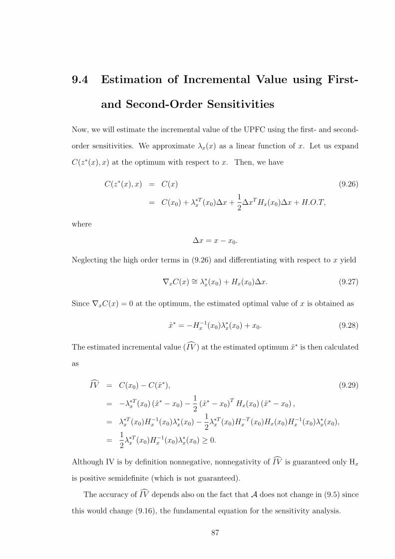
9.4 Estimation of Incremental Value using First-
and Second-Order Sensitivities
Now, we will estimate the incremental value of the UPFC using the first- and second-
order sensitivities. We approximate λx(x) as a linear function of x. Let us expand
C(z∗(x), x) at the optimum with respect to x. Then, we have
C(z∗(x), x) = C(x) (9.26)
= C(x0) + λ∗Tx (x0)∆x +1
2∆xT Hx(x0)∆x + H.O.T,
where
∆x = x− x0.
Neglecting the high order terms in (9.26) and differentiating with respect to x yield
∇xC(x) ∼= λ∗x(x0) + Hx(x0)∆x. (9.27)
Since ∇xC(x) = 0 at the optimum, the estimated optimal value of x is obtained as
x∗ = −H−1x (x0)λ
∗x(x0) + x0. (9.28)
The estimated incremental value (IV ) at the estimated optimum x∗ is then calculated
as
IV = C(x0)− C(x∗), (9.29)
= −λ∗Tx (x0) (x∗ − x0)− 1
2(x∗ − x0)
T Hx(x0) (x∗ − x0) ,
= λ∗Tx (x0)H−1x (x0)λ
∗x(x0)− 1
2λ∗Tx (x0)H
−Tx (x0)Hx(x0)H
−1x (x0)λ
∗x(x0),
=1
2λ∗Tx (x0)H
−1x (x0)λ
∗x(x0) ≥ 0.
Although IV is by definition nonnegative, nonnegativity of IV is guaranteed only Hx
is positive semidefinite (which is not guaranteed).
The accuracy of IV depends also on the fact that A does not change in (9.5) since
this would change (9.16), the fundamental equation for the sensitivity analysis.
87

CHAPTER 10
RESULTS
10.1 Result of Sensitivity Analysis
The proposed sensitivity methods are tested on a 5-bus system derived from the IEEE
14-bus system, and IEEE 14- and 30-bus systems to establish their effectiveness.
These systems have 7, 20, 41 transmission lines, respectively. Figure 10.1 shows the
5-bus system [15]. The system consists of two generators at buses 1 & 2 and one
synchronous condenser at bus 3. We assume that generator 2 has higher generation
cost than generator 1, and UPFCs are installed in the middle of each transmission
line. Loads are assigned such that the current flow constraint in line 1 is binding (we
assume that thermal constraints limit line flow for this example).
The marginal values (|λT |, |λφ| and |λρ|), estimated incremental values (IV ) and
Figure 10.1: Diagram of 5-bus subset of IEEE 14-bus system [15]
88

1 2 3 4 5 6 70
2
4
6
8
10
12
Line number
MV
/ A
ctua
l IV
λT/15
λφ/15
λρ/5
Estimated IVActual IV ($/hr)
Figure 10.2: Normalized marginal and incremental values for 5-bus system.
actual incremental values (IV ) for the 5-bus system are shown in Figure 10.2. It
shows that the lines with high MVs usually produce high estimated IVs. The UPFC
location in line 1 produces high MVs for |λT | and |λφ|, and the highest estimated IV.
In general, it is more economical to locate the UPFC in heavily-loaded high voltage
PG1 PG2 Ploss Est. IV Actual IVUPFC Location MW MW MW $/hr $/hrWithout UPFC 198.18 71.60 10.51 0 0
Line 1 219.31 51.18 11.64 11.85 6.90Line 2 224.56 46.19 11.90 7.69 6.38Line 3 196.85 72.77 10.77 1.13 0.73Line 4 202.45 67.40 10.99 1.97 1.83Line 5 204.52 65.44 11.11 2.17 2.07Line 6 196.85 72.73 10.73 0.75 0.67Line 7 202.59 67.22 10.95 0.78 0.80
Table 10.1: Real power generation, line loss and total generation cost for 5-bus system
89

0 2 4 6 8 10 12 14 16 18 200
2
4
6
8
10
12
Line number
MV
λT/15
λφ/15
λρ/5
0 2 4 6 8 10 12 14 16 18 200
2
4
6
8
Line number
IV
Estimated IV ($/hr)Actual IV ($/hr)
Figure 10.3: Marginal and incremental values for IEEE 14-bus system.
line 1 since it allows more power to be transmitted in under-utilized line 2 while
preventing line 1 from overloading. Eventually, no further savings due to UPFC
operation can be achieved because of the voltage constraint at bus-2.
Also, reasonable agreement can be observed between the estimated IVs and the
actual IVs except line 1 and line 2. The difference between the estimated IV and the
actual IV is attributed to the fact that some inequality constraints become binding so
that the UPFC cannot be fully utilized. Thus, it is important that the set of binding
constraints does not change as x changes in order to obtain a reliable estimated IV.
(However, we cannot actually verify this without many additional OPF solutions).
For the 5-bus case, Table 10.1 shows real power generations, transmission line
losses and incremental values. Since the generation marginal cost, adjusted for
marginal losses at bus 1 is lower than that at bus 2, it is profitable to obtain more
90
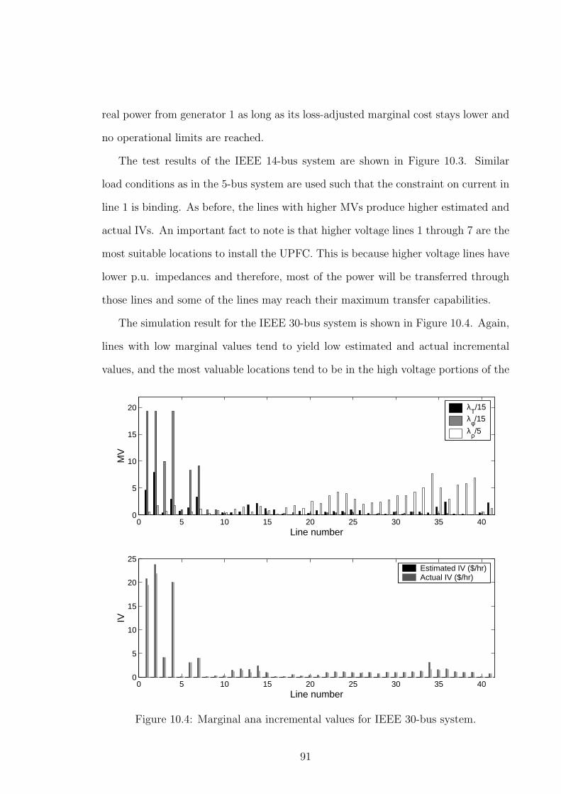
real power from generator 1 as long as its loss-adjusted marginal cost stays lower and
no operational limits are reached.
The test results of the IEEE 14-bus system are shown in Figure 10.3. Similar
load conditions as in the 5-bus system are used such that the constraint on current in
line 1 is binding. As before, the lines with higher MVs produce higher estimated and
actual IVs. An important fact to note is that higher voltage lines 1 through 7 are the
most suitable locations to install the UPFC. This is because higher voltage lines have
lower p.u. impedances and therefore, most of the power will be transferred through
those lines and some of the lines may reach their maximum transfer capabilities.
The simulation result for the IEEE 30-bus system is shown in Figure 10.4. Again,
lines with low marginal values tend to yield low estimated and actual incremental
values, and the most valuable locations tend to be in the high voltage portions of the
0 5 10 15 20 25 30 35 400
5
10
15
20
Line number
MV
λT/15
λφ/15
λρ/5
0 5 10 15 20 25 30 35 400
5
10
15
20
25
Line number
IV
Estimated IV ($/hr)Actual IV ($/hr)
Figure 10.4: Marginal ana incremental values for IEEE 30-bus system.
91

system. Figure 10.4 also shows that estimated IVs are quite close to actual IVs. In
addition, we see that locations with large incremental values are also those with large
marginal values, thus supporting the idea of using only first-order sensitivity analysis
to screen for promising locations for installation of a UPFC.
10.2 Result of GEOPF
This section contains case studies that evaluate the capability of the GEOPF in
maximizing social welfare associated with electricity generation cost, gas supply cost,
and gas and electricity consumer’s benefit. The coefficients of quadratic generation
cost and benefit curves are summarized in Appendix C. Since combined nodes are
considered as nodes which simply convert gas energy to electric energy, these nodes
are not associated with generation cost and gas consumer’s benefit. Instead, we will
Figure 10.5: Combined gas and electric network
92
use the coefficients of the fuel rate curve for the gas-fired generator to calculate the
amount of gas supplied to the combined node.
10.2.1 Test System I
We will first consider a simple combined network with two real power generators,
one of which is a gas-fired generator and the other is a coal-fired generator. Tie-line
connections in both natural gas and electricity networks are not considered in this
test system. The system analyzed is a combined natural gas and electricity network,
which consists of a 5-bus system and a 15-node gas system, as shown in Figure 10.5.
The 15-node system is a modification of an example system in [22], plus some made-
up benefit and cost functions. The 5-bus electric system obtained by modifying the
IEEE 14-bus system has two real power generators at buses 1 and 2, one synchronous
condenser at bus 3, and four loads at buses 2 through 5, and bus 1 serves as the
reference/slack bus in the electric network. The generator at bus 2 is coincident with
gas network node 15. We assume that node 1 is the known-pressure node in the gas
system. The gas network has fifteen nodes consisting of five loads at nodes 3, 4, 13,
14, and 15, two sources at nodes 1 and 2, and eight compressor inlet-outlet nodes
5 through 12. We assume that the compressors in the gas network are driven by
gas turbines, and the gas is tapped from the outlet node of the compressor station.
Appendix C shows the input data for gas and electricity network represented in Figure
10.5.
We assume that generator 1 uses coal with a fixed price, and generator 2 uses
natural gas with high price variations.
To study the impact of the wellhead gas prices at source nodes 1 and 2 to the real
power generation at combined node 15, three test conditions with different wellhead
gas prices are considered as follows:
93
Case 1:
Wellhead gas price at node 1 = $2.07 /(106× BTU)
Wellhead gas price at node 2 = $2.12 /(106× BTU)
Case 2:
Wellhead gas price at node 1 = $2.46 /(106× BTU)
Wellhead gas price at node 2 = $2.71 /(106× BTU)
Case 3: (pipeline branch between nodes 12 and 14 removed)
Wellhead gas price at node 1 = $2.46 /(106× BTU)
Wellhead gas price at node 2 = $2.71 /(106× BTU)
Wellhead gas prices in cases 2 and 3 are higher than those in case 1. Table 10.2
shows simulation results for the three case studies. In case 1, the gas-fired generator
reaches its maximum generation limit due to the low gas price at combined node
15. As noted in Table 10.2, the optimal real power generation PG2 at the combined
node is quite sensitive to the wellhead gas prices, and reduced greatly as the wellhead
gas prices increase. In case 3, we assume that the pipeline branch between nodes
12 and 14 is unavailable due to a forced-outage. The gas-fired generator reaches its
minimum generation limit, which indicates that contingencies occurring in the gas
network may result in the significant change of electricity generation patterns. Now,
let us compare the social welfare of non-integrated gas and electricity operation with
that obtained from the GEOPF for case 2. The social welfare from the GEOPF is
$22,405.83/hr, and the gas price at node 15 is $2.82/(106×BTU). For non-integrated
network operation, let’s say that there is a broker who purchases gas from node 15,
and sells it to the gas-fired generator at bus 2. He has a long-term contract with
the gas-fired generator that he will supply gas at a fixed price. (obviously other
contractual arrangements are possible.) But, he will purchase gas from the spot
market in the gas network. Thus, the broker can make profit by the price difference
94

times the amount of gas sold. With the prices of coal and natural gas given, the OPF
is implemented to obtain social welfare maximizing solutions in the electric network.
Then, the amount of gas transformed to electrical energy at the combined node is
used as equality constraint in the OGF problem to calculate the optimal gas network
operation scheme. Figure 10.6 shows social welfare losses if we optimize two networks
by individually running OPF and OGF with different gas prices at node 15. Since
the broker is involved for non-integrated operation, the social welfare is calculated by
SW = SWE + SWG + BB, (10.1)
where
SWE = electric network social welfare,
SWG = gas network social welfare,
BB = broker’s benefit (profit).
Figure 10.6 indicates that the social welfare loss becomes zero when the gas price
at node 15 is $2.82/(106×BTU), which is the same as the marginal cost of gas at
node 15 obtained from the GEOPF. Thus, we can verify that the GEOPF returns
the social welfare maximizing solutions for the combined gas and electricity network.
Since the broker maintains a price difference between the gas price at node 15 and
the gas price at the generator at bus 2, the social welfare is reduced even though the
difference between payments from the electric system to the gas system exactly cancel
out in the overall social welfare, but prices are distorted from their optimal values.
Other contractual arrangements with the broker might result in different outcomes.
10.2.2 Test System II
We have seen in Figure 10.6 that we can obtain optimal solutions for the GEOPF
by individually running the OPF and the OGF. However, if there are more than one
95
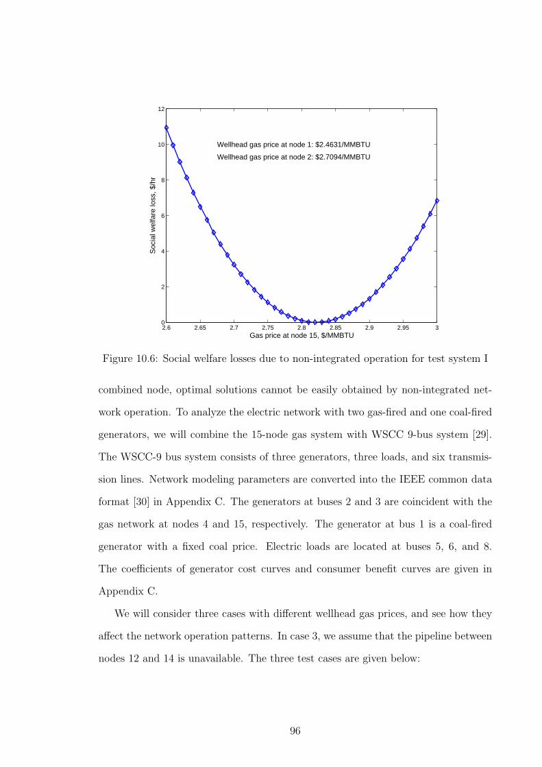
2.6 2.65 2.7 2.75 2.8 2.85 2.9 2.95 30
2
4
6
8
10
12
Gas price at node 15, $/MMBTU
Soc
ial w
elfa
re lo
ss, $
/hr
Wellhead gas price at node 1: $2.4631/MMBTU
Wellhead gas price at node 2: $2.7094/MMBTU
Figure 10.6: Social welfare losses due to non-integrated operation for test system I
combined node, optimal solutions cannot be easily obtained by non-integrated net-
work operation. To analyze the electric network with two gas-fired and one coal-fired
generators, we will combine the 15-node gas system with WSCC 9-bus system [29].
The WSCC-9 bus system consists of three generators, three loads, and six transmis-
sion lines. Network modeling parameters are converted into the IEEE common data
format [30] in Appendix C. The generators at buses 2 and 3 are coincident with the
gas network at nodes 4 and 15, respectively. The generator at bus 1 is a coal-fired
generator with a fixed coal price. Electric loads are located at buses 5, 6, and 8.
The coefficients of generator cost curves and consumer benefit curves are given in
Appendix C.
We will consider three cases with different wellhead gas prices, and see how they
affect the network operation patterns. In case 3, we assume that the pipeline between
nodes 12 and 14 is unavailable. The three test cases are given below:
96

Figure 10.7: Combined gas and electric network
Case 1:
Wellhead gas price at node 1 = $2.07 /(106× BTU)
Wellhead gas price at node 2 = $2.12 /(106× BTU)
Case 2:
Wellhead gas price at node 1 = $2.51 /(106× BTU)
Wellhead gas price at node 2 = $2.51 /(106× BTU)
Case 3: (pipeline branch between nodes 12 and 14 removed)
Wellhead gas price at node 1 = $2.07 /(106× BTU)
Wellhead gas price at node 2 = $2.12 /(106× BTU)
Table 10.3 shows the GEOPF results for three test cases. The coal-fired generator
reaches its minimum generation limit since the wellhead gas prices are relatively low
in case 1. As the wellhead gas prices increase, the generation patterns are changed
noticeably as in case 2. In addition, the amount of gas production at each source node
97

2.46 2.48 2.5 2.52 2.54 2.56
2.52.52
2.542.56
2.582.6
0
5
10
15
20
Gas price at node 4, $/MMBTUGas price at node 15, $/MMBTU
Wellhead gas price at node 1:$2.51/MMBTU
Wellhead gas price at node 2:$2.51/MMBTU
Soc
ial W
elfa
re L
oss,
$/h
r
Figure 10.8: Social welfare losses due to non-integrated operation for test system II
varies significantly depending on the wellhead gas prices. The electric generation at
bus 3 is significantly reduced due to high gas price at node 15. In case 3, we can see
that the generation pattern is changed noticeable due to the gas transmission line
outage.
Now, we will compare the social welfare of non-integrated gas and electricity op-
eration with that obtained from the GEOPF for case 2. Due to having to guess the
gas prices at the two combined nodes for non-integrated gas and electricity operation,
the social welfare maximizing solution cannot be easily obtained by individually run-
ning OPF and OGF. Figure 10.8 shows the social welfare losses if two networks are
operated individually. We can see that the social welfare loss is zero when the gas
prices at nodes 4 and 15 are $2.52/(106×BTU) and $2.55/(106×BTU), respectively.
These gas prices are the same gas prices as we obtained from the GEOPF, which
verify that the GEOPF can find global solutions which maximize the social welfare
for the combined gas and electricity network.
98

Case 1 Case 2 Case 3Gas supply (106×SCF/hr)
wS1 7.2970 8.9047 6.3694wS2 10.079 5.1950 6.7761
Source pressure (psia)π1 (slack) 1000.000 1000.000 1000.000
π2 1200.000 723.167 1057.119Gas load demand (106×SCF/hr)
wL3 3.8294 3.2460 3.2342wL4 3.9981 3.3570 3.3570wL13 4.2388 3.5142 3.1343wL14 4.2474 3.4329 2.9930wL15 0.9891 0.4710 0.3438
Gas price ($/(106×BTU)MC3 2.1238 2.6978 2.7094MC4 2.1271 2.7094 2.7094MC13 2.1872 2.8205 3.1525MC14 2.1873 2.8205 3.1625MC15 2.1885 2.8213 3.1578
Real power generation (MW)PG1 132.296 193.713 188.8408PG2 150.000 41.786 15.000
Real power demand (MW)PL2 23.1602 18.1988 14.8824PL3 99.1564 81.8019 70.4640PL4 96.3892 80.6280 70.4423PL5 54.0011 45.7602 40.4425
Electricity price ($/MWh)MC1 11.2170 11.3177 11.3097MC2 11.4850 13.6154 15.0395MC3 12.4696 14.3126 15.5167MC4 12.2137 13.8824 14.9615MC5 12.0377 13.5610 14.5447
Social welfare ($/hr)CE 2161.93 2853.94 2798.81BE 4735.93 4129.35 3690.53CG 36,994.15 36,548.16 34,557.75BG 65,504.01 58,591.45 56,071.87SW 31,083.86 23,318.70 22,405.83
Table 10.2: GEOPF results for test system I
99

Case 1 Case 2 Case 3Gas supply (106×SCF/hr)
wS1 7.2883 4.3160 6.0010wS2 6.8673 7.8251 5.7177
Source pressure (psia)π1 (slack) 1000.000 1000.000 1000.000
π2 978.630 1200.000 1043.454Gas load demand (106×SCF/hr)
wL3 3.8377 3.4274 3.8350wL4 1.2177 0.8232 1.3102wL13 4.2628 3.8281 3.3177wL14 4.2743 3.7857 3.0599wL15 0.5012 0.2629 0.1212
Gas price ($/(106×BTU)MC3 2.1156 2.5193 2.1182MC4 2.1182 2.5197 2.1182MC13 2.1663 2.5462 2.9922MC14 2.1663 2.5463 3.1105MC15 2.1669 2.5465 3.0493
Real power generation (MW)PG1 21.6000 87.3278 30.4071PG2 252.8145 171.9092 271.6400PG3 102.9182 54.1304 25.0000
Real power demand (MW)PL5 129.2073 122.4114 123.2469PL6 112.4537 82.7093 85.8920PL8 125.4047 104.5075 109.6712
Electricity price ($/MWh)MC1 11.5305 12.8552 12.7619MC2 10.5436 12.3989 11.8022MC3 10.7675 12.5898 12.2628MC5 11.5429 12.9922 12.7957MC6 11.6100 13.0129 12.8585MC8 10.7830 13.0129 12.1386
Social welfare ($/hr)CE 274.96 1116.37 387.29BE 6884.63 6189.05 6305.11CG 30,070.20 30,959.73 24,895.15BG 49,634.46 46,460.98 43,902.35SW 26,173.92 20,573.94 24,925.02
Table 10.3: GEOPF results for test system II
100

CHAPTER 11
CONCLUSIONS AND FUTURE WORK
The objective of this dissertation were:
• to propose an integrated analysis and solution to the GEOPF problem for com-
bined natural gas and electric power transmission networks from a central plan-
ning point of view,
• to develop a screening technique to optimally locate UPFCs and other FACTS
devices, and
• to introduce a new model for an ideal UPFC to facilitate solution of OPF
problems.
The use of an integrated methodology might not seem to make much sense due
to the separation of the gas and electricity markets. However, once an integrated
methodology is developed, we can then begin work on a distributed or parallel imple-
mentation of the centralized problem (which we must already know how to solve if the
required data were available). The GEOPF solution is especially important if there
are multiple combined nodes (gas-fired generators). Since electric energy and gas
prices are so volatile, the GEOPF will significantly contribute to achieving optimal
system operation for the combined gas and electric network.
We have also developed a new technique to estimate the UPFC value by using
the first- and second-order sensitivities. As demonstrated by several test systems,
101

transmission lines with higher MVs with respect to the UPFC control parameters
yield higher estimated and actual IVs. The estimated IV seems to give a good ap-
proximation to the actual IV when the binding inequality set does not change as the
UPFC control parameters are relaxed. Simulation results also revealed that lines with
low estimated IV yield low actual IV, which adds to the credibility of the sensitivity
analyses. We can apply this sensitivity technique to screen for the optimal location
of a UPFC in a large power system by ignoring transmission lines with low MV and
low estimated IV, and performing a full OPF simulation only with lines with higher
estimated IV to obtain the actual IV. Thus, this technique can significantly reduce
the computational burden of determining optimal locations of UPFC in a large power
system.
To implement the first- and second-order sensitivities of the UPFC to find optimal
locations, we developed a unique UPFC ideal transformer model, which consists only
of an ideal transformer with a complex turns ratio and a variable shunt admittance.
Since this model is embedded in the Ybus matrix, the size of the Ybus matrix is not
changed, and the MV and estimated IV for each transmission line can be obtained
from the solution of the single base case OPF.
Regarding UPFC sensitivity analysis, future work should determine the optimal
location x within each line ik should be determined. In addition, λT , λφ and λρ need
to be transformed to directly represent the marginal values of the series capacitor and
VAR compensator. Loadflow and OPF applications using the UPFC ideal transformer
model need to be explored. Inclusion of non-ideal UPFC behavior should also be
included in future work.
Note that the GEOPF solution and/or use of proposed UPFC model also pro-
vides optional short-term operational solutions, in addition to long-term signals for
investment in new facilities.
102

Future work should be focused on financial tools for valuation of financial deriva-
tives (such as call options) in conjunction with the GEOPF to determine the value of
new or existing assets, as well as the role of brokers as intermediaries between gas and
electric utilities. The available financial tools have not been combined in the inte-
grated manner needed for proper operation and planning of combined gas and electric
systems. The technique for evaluating investments for gas and electric projects in a
competitive market are fairly new, and relatively little quantitative data are avail-
able on competitive prices and their volatilities. Hence, the valuation of assets in a
competitive market is important for future investment decisions in the competitive
market. As mentioned above, work on a distributed implementation of the centralized
solution-including market design-is also a goal of future work in this area.
103
BIBLIOGRAPHY
[1] Michael Klein. Competition in network industries. Technical report, The World
Bank Private Sector Development Department, April 1996.
[2] Harry Singh. The art of market design-what’s next for power markets and SMD?
IEEE Power & Energy Magazine, pages 12–16, September/October 2003.
[3] Marija Ilic, Francisco Galiana, and Lester Fink. Power Systems Resturcturing
(Engineering and Economics). Kluwer Academic Publishers, 1998.
[4] Colin Schauder. The unified power flow controller - a concept becomes reality.
In IEE Colloquium on Flexible AC Transmission Systems-The FACTS(Ref. No.
1998/500), pages 7/1–7/6, November 1998.
[5] L. Gyugyi, C. D. Schauder, S. L. Williams, T. R. Rietman, D. R. Torgerson,
and A. Edris. The unified power flow controller: A new approach to power
transmission control. IEEE Transactions on Power Delivery, 10(2):1085–1097,
April 1995.
[6] M. Noroozian, L. Angquist, M. Ghandhari, and G. Andersson. Use of UPFC for
optimal power flow control. IEEE Transactions on Power Delivery, 12(4):1629–
1634, October 1997.
[7] L. Gyugyi. Unified power-flow control concept for flexible AC transmission sys-
tems. In IEE Proceedings C. on Generation, Transmission and Distribution,
volume 139(4), pages 323–331, July 1992.
104

[8] Thomas W. Gedra. Power Economics and Regulation. Class notes for ECEN
5193 at Oklahoma State University, 2004.
[9] J. Duncan Glover and Mulukutla Sarma. Power System Analysis & Design. PWS
Publishing Company, third edition, 2002.
[10] John J. Grainger and Jr. William D. Stevenson. Power System Analysis.
McGraw-Hill, Inc., 1994.
[11] Allen J. Wood and Bruce F. Wollenberg. Power Generation, Operation, and
Control. John Wilen & Sons. Inc., second edition, 1996.
[12] Parnjit Damrongkulkamjorn. Optimal Power Flow with Expected Security Costs.
PhD thesis, Oklahoma State University, May 1999.
[13] Stephen J. Wright. Primal-Dual Interior-Point Methods. SIAM: Society for
Industrial and Applied Mathematics, 1997.
[14] Seungwon An and Thomas W. Gedra. Estimation of UPFC value using sensi-
tivity analysis. In Proceedings of the 2002 Midwest Symposium on Circuits and
Systems, Oklahoma State University, Tulsa, OK, August 2002.
[15] Parnjit Damrongkulkamjorn, Prakash K. Arcot, Peter Dcouto, and Thomas W.
Gedra. A screening technique for optimally locating phase shifters in power
systems. In Proceedings of the IEEE/PES Transmission and Distribution Con-
ference, pages 233–238, April 1994.
[16] James Danel Weber. Implementation of a newton-based optimal power flow into
a power system simulation environment. Master’s thesis, University of Illinois at
Urbana-Champaign, 1997.
105

[17] K. Ponnambalam, V.H. Quintana, and A. Vannelli. A fast algorithm for power
system optimization problems using an interior point method. IEEE Transac-
tions on Power Systems, 7(2):892 –899, 1992.
[18] Yu-Chi Wu, Debs, A.S., and R.E. Marsten. A direct nonlinear predictor-corrector
primal-dual interior point algorithm for optimal power flows. IEEE Transactions
on Power Systems, 9(2):876–883, 1994.
[19] N. Karmarkar. A new polynomial-time algorithm for linear programming. Com-
binatorica, 4:373–395, 1984.
[20] Stephen G. Nash and Ariela Sofer. Linear and Nonlinear Programming. The
McGraw-Hill Companies, Inc., 1996.
[21] Roland W. Jeppson. Analysis of Flow in Pipe Networks. ANN Arbor Science,
1976.
[22] Andrzej J. Osiadacz. Simulation and Analysis of Gas Network. Gulf Publishing
Company, February 1987.
[23] Festus Oladele Olorunntwo. Natural Gas Transmission System Optimization.
PhD thesis, The University of Texas at Austin, May 1981.
[24] E. W. McAllister. Pipeline Rule of Thumb Handbook. Gulf Publishing Company,
second edition, 1988.
[25] T. R Weymouth. Problems in natural gas engineering. ASME Transactions,
34:185–234, 1942.
[26] Lloyd N. Trefethen and III David Bau. Numerical Linear Algebra. SIAM (Society
for Industrial and Applied Mathematics), 1996.
[27] Seungwon An and Thomas W. Gedra. UPFC ideal transformer model. In Pro-
ceedings of North American Power Symposium, pages 46–50, October 2003.
106

[28] Hal R. Varian. Microeconomic Analysis. New York: Norton, third edition, 1992.
[29] Peter W. Sauer and M.A. Pai. Power Systems Dynamics and Stability. Prentice
Hall, 1997.
[30] Working Group on a Common Format for Exchange of Solved Load Flow Data.
Common format for exchange of solved load flow data. IEEE Transactions
on Power Apparatus and Systems, PAS-92(6):1916–1925, November/December
1973.
107

APPENDIX A
DERIVATIVES REQUIRED FOR GEOPF
Appendix A includes the Jacobian and Hessian matrixes required to construct math-
ematical equations to solve the GEOPF.
A.1 Electric Networks
• Voltage Magnitudes and Angles at Each Bus
V =
V1
V2
...
VNB
, ejθ =
ejθ1
ejθ2
...
ejθNB
, ~V =
V1ejθ1
V2ejθ2
...
VNBejθNB
• Current Injection at Each Bus
~Ii =
[NB∑
k=1
Ybusik~Vk
]∗, i = 1, · · · , NB
~I =
~I1
~I2
...
~INB
108
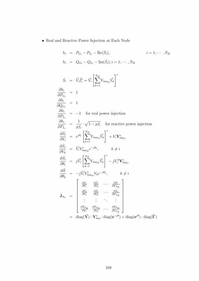
• Real and Reactive Power Injection at Each Node
hi = PGi− PLi
− Re(Si), i = 1, · · · , NB
hi = QGi−QLi
− Im(Si), i = 1, · · · , NB
Si = ~Vi~I∗i = ~Vi
[NB∑
k=1
Ybusik~Vk
]∗
∂hi
∂PGi
= 1
∂hi
∂QGi
= 1
∂hi
∂PLi
= −1 for real power injection
∂hi
∂PLi
=1
pfi
·√
1− pfi for reactive power injection
∂Si
∂Vi
= ejθi
[NB∑
k=1
Ybusik~Vk
]∗+ ViY
∗busii
∂Si
∂Vk
= ~ViY∗busik
e−jθk , k 6= i
∂Si
∂θi
= j~Vi
[NB∑
k=1
Ybusik~Vk
]∗− jV 2
i Y∗busii
∂S
∂θk
= −j~ViY∗busik
Vke−jθk , k 6= i
JSV=
∂S1
∂V1
∂S1
∂V2· · · ∂S1
∂VNB
∂S2
∂V1
∂S2
∂V2· · · ∂S2
∂VNB
......
. . ....
∂SNB
∂V1
∂SNB
∂V2· · · ∂SNB
∂VNB
= diag(~V) ·Y∗bus · diag(e−jθ) + diag(ejθ) · diag(~I∗)
109
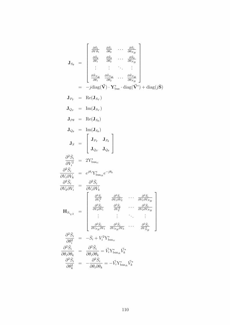
JSθ=
∂S1
∂V θ1
∂S1
∂θ2· · · ∂S1
∂θNB
∂S2
∂θ1
∂S2
∂θ2· · · ∂S2
∂θNB
......
. . ....
∂SNB
∂θ1
∂SNB
∂θ2· · · ∂SNB
∂θNB
= −jdiag(~V) ·Y∗bus · diag(~V∗) + diag(jS)
JPV= Re(JSV
)
JQV= Im(JSV
)
JPθ = Re(JSθ)
JQθ= Im(JSθ
)
JS =
JPVJPθ
JQVJQθ
∂2Si
∂V 2i
= 2Y∗busii
∂2Si
∂Vi∂Vk
= ejθiY∗busik
e−jθk
∂2Si
∂Vk∂Vi
=∂2Si
∂Vi∂Vk
HSiV 2
=
∂2Si
∂V 21
∂2Si
∂V1∂V2· · · ∂2Si
∂V1∂VNB
∂2Si
∂V2∂V1
∂2Si
∂V 22
· · · ∂2Si
∂V2∂VNB
......
. . ....
∂2Si
∂VNB∂V1
∂2Si
∂VNB∂V2
· · · ∂2Si
∂V 2NB
∂2Si
∂θ2i
= −Si + V 2i Y∗
busii
∂2Si
∂θi∂θk
=∂2Si
∂θi∂θk
= ~ViY∗busik
~V ∗k
∂2Si
∂θ2k
= − ∂2Si
∂θi∂θk
= −~ViY∗busik
~V ∗k
110

HSiθ2
=
∂2Si
∂θ21
∂2Si
∂θ1∂θ2· · · ∂2Si
∂θ1∂θNB
∂2Si
∂θ2∂θ1
∂2Si
∂θ22
· · · ∂2Si
∂θ2∂θNB
......
. . ....
∂2Si
∂θNB∂θ1
∂2Si
∂θNB∂θ2
· · · ∂2Si
∂θ2NB
∂2Si
∂Vi∂θi
=∂2Si
∂θi∂Vi
= jejθi
[NB∑
k=1
Ybusik~Vk
]∗− jViY
∗busii
∂2Si
∂Vi∂θk
=∂2Si
∂θk∂Vi
= −jejθiY∗busik
~V ∗k
∂2Si
∂Vk∂θi
=∂2Si
∂θi∂Vk
= j~ViY∗busik
e−jθk
∂2Si
∂Vk∂θk
=∂2Si
∂θk∂Vk
= −j~ViY∗busik
e−jθk
HSiV θ=
∂2Si
∂V1∂θ1
∂2Si
∂V1∂θ2· · · ∂2Si
∂V1∂θNB
∂2Si
∂V2∂θ1
∂2Si
∂V2∂θ2· · · ∂2Si
∂V2∂θNB
......
. . ....
∂2Si
∂VNB∂θ1
∂2Si
∂θNB∂θ2
· · · ∂2Si
∂VNB∂θNB
HSiθV= HT
SiV θ
HPi= Re
HSiV 2
HSiV θ
HSiθVHSi
θ2
HQi= Im
HSiV 2
HSiV θ
HSiθVHSi
θ2
• Reference Angle Equality Constraint
hi = θi, i = reference bus
∂hi
∂θi
= 1
111
• Equality Constraints at Combined Buses
hi = wLi− (
αGi+ βGi
PGiSbase + γGi
P 2Gi
S2base
) 1
GHV,
i = 1, . . . , NGE
∂hi
∂wLi
= 1
∂hi
∂PGi
= −(βGiSbase + 2γGi
PGiS2
base)1
GHV
∂2hi
∂P 2Gi
= −2γGiS2
base
1
GHV
• Voltage Magnitude Limit
gi = Vmini− Vi, i = 1, . . . , NB
∂gi
∂Vi
= −1
gi = Vi − Vmaxi, i = 1, . . . , NB
∂gi
∂Vi
= 1
• Real Power Generation Limit
gi = PG mini− PGi
, i = 1, . . . , NPG
∂gi
∂PGi
= −1
gi = PGi− PG maxi
, i = 1, . . . , NPG
∂gi
∂PGi
= 1
• Real Power Load Limit
gi = −PLi, i = 1, . . . , NEL
∂gi
∂PLi
= −1
112

• Reactive Power Generation Limit
gi = QG mini−QGi
, i = 1, . . . , NQG
∂gi
∂QGi
= −1
gi = QGi−QG maxi
, i = 1, , . . . , NQG
∂gi
∂QGi
= 1
• Line Flow Limit
gi = ~Iik · ~I∗ik − |Iik|2 , i = 1, . . . , NEB
~Iik =(
~Vi − ~Vk
)Yik + Yshuntik
~Vi
∂~Iik
∂Vi
= ejθiYik + Yshuntikejθi
∂~Iik
∂Vk
= −ejθkYik
∂~Iik
∂θi
= j~Vi (Yik + Yshuntik)
∂~Iik
∂θk
= −j~VkYik
∂~Iik~I∗ik
∂Vi
= ~Iik∂~I∗ik∂Vi
+ ~I∗ik∂~Iik
∂Vi
∂~Iik~I∗ik
∂Vk
= ~Iik∂~I∗ik∂Vk
+ ~I∗ik∂~Iik
∂Vk
∂~Iik~I∗ik
∂θi
= ~Iik∂~I∗ik∂θi
+ ~I∗ik∂~Iik
∂θi
∂~Iik~I∗ik
∂θk
= ~Iik∂~I∗ik∂θk
+ ~I∗ik∂~Iik
∂θk
∂2~Iik
∂θ2i
= −~Vi (Yik + Yshuntik)
∂2~Iik
∂θ2k
= −jejθkYik
113

∂2~Iik
∂Vi∂θi
=∂2~Iik
∂θi∂Vi
= jejθi (Yik + Yshuntik)
∂2~Iik
∂Vk∂θk
=∂2~Iik
∂Vk∂θk
= −jejθkYik
∂2~Iik~I∗ik
∂V 2i
= 2∂~Iik
∂Vi
∂~I∗ik∂Vi
∂2~Iik~I∗ik
∂V 2k
= 2∂~Iik
∂Vk
∂~I∗ik∂Vk
∂2~Iik~I∗ik
∂θ2i
= ~Iik∂2~I∗ik∂θ2
i
+ 2∂~Iik
∂θi
∂~I∗ik∂θi
+ ~I∗ik∂2~Iik
∂θ2i
∂2~Iik~I∗ik
∂θ2k
= ~Iik∂2~I∗ik∂θ2
k
+ 2∂~Iik
∂θk
∂~I∗ik∂θk
+ ~I∗ik∂2~Iik
∂θ2k
∂2~Iik~I∗ik
∂Vi∂θi
=∂2~Iik
~I∗ik∂θi∂Vi
= ~Iik∂2~I∗ik
∂Vi∂θi
+∂~Iik
∂Vi
∂~I∗ik∂θi
+∂~I∗ik∂Vi
∂~Iik
∂θi
+ ~I∗ik∂2~Iik
∂Vi∂θi
∂2~Iik~I∗ik
∂Vk∂θk
=∂2~Iik
~I∗ik∂θk∂Vk
= ~Iik∂2~I∗ik
∂Vk∂θk
+∂~Iik
∂Vk
∂~I∗ik∂θk
+∂~I∗ik∂Vk
∂~Iik
∂θk
+ ~I∗ik∂2~Iik
∂Vk∂θk
∂2~Iik~I∗ik
∂Vi∂θk
=∂2~Iik
~I∗ik∂θk∂Vi
=∂~Iik
∂Vi
∂~I∗ik∂θk
+∂~I∗ik∂Vi
∂~Iik
∂θk
∂2~Iik~I∗ik
∂Vk∂θi
=∂2~Iik
~I∗ik∂θi∂Vk
=∂~Iik
∂Vk
∂~I∗ik∂θi
+∂~I∗ik∂Vk
∂~Iik
∂θi
114
A.2 Gas Network
• Gas Pressures and Branch Flow Rates
π =
[π1 π2 . . . πNN
]T
f =
[f1 . . . fNP
fNP +1 . . . fNP +NC
]T
• Gas Consumption Rates and Horsepowers at Compressor Stations
τ =
[τ1 τ2 . . . τNC
]T
H =
[H1 H2 . . . HNC
]T
• Weymouth Flow Equation for Pipeline Branches
hk = hkij= π2
i − π2j −
(1
Mk
)m1
(Sijfkij)m1Sij, k = 1, . . . , NP
Sij = sign(fkij
)
∂hk
∂πi
= 2πi
∂hk
∂πj
= −2πj
∂hk
∂fkij
= −m1
(1
Mk
)m1
(Sijfkij)(m1−1)
∂2hk
∂π2i
= 2
∂2hk
∂π2j
= −2
∂2hk
∂f 2kij
= −m1(m1− 1)
(1
Mk
)m1
f(m1−2)kij
Sij
• Reference Pressure Equality Constraints
hi = πi − πset, i = reference node
∂hi
∂πi
= 1
115
• Compressor Operation Equality Constraints
hk = hkij= Hk −Bkfk
[(πj
πi
)Rk
− 1
], k = 1, . . . , NC
Rk = Zki
α− 1
α∂hk
∂Hk
= 1
∂hk
∂πi
= RkBkfkπRkj π
−(Rk+1)i
∂hk
∂πj
= −RkBkfkπ(Rk−1)j π−Rk
i
∂hk
∂fk
= −Bk
[(πj
πi
)R
k
− 1
]
∂2hk
∂π2i
= −Rk(Rk + 1)BkfkπRkj π
−(Rk+2)i
∂2hk
∂π2j
= −Rk(Rk − 1)Bkfkπ(Rk−2)j π−Rk
i
∂2hk
∂πi∂πj
=∂2hk
∂πj∂πi
= R2kBkfkπ
(Rk−1)j π
−(Rk+1)i
∂2hk
∂fk∂πi
=∂2hk
∂πi∂fk
= RkBkπRkj π
−(Rk+1)i
∂2hk
∂fk∂πj
=∂2hk
∂πj∂fk
= −RkBkπ(Rk−1)j π−Rk
i
hk = hkij= τk −
(αTk
+ βTkHkij
+ γTkH2
kij
), k = 1, . . . , NC
∂hk
∂τk
= 1
∂hk
∂Hkij
= −βTk− 2γTk
Hkij
∂2hk
∂H2kij
= −2γTk
116

• Nodal-Flow Balance Equation
h = (A + U)f + w −Tτ, dim(h) = NN × 1
∂h
∂f= A + U
∂h
∂τ= −T
∂hi
∂wSi
=
+1, if a source is connected to node i,
0, otherwise.
∂hi
∂wLi
=
−1, if a load is connected to node i,
0, otherwise.
• Compressor Inlet-Outlet Pressure Inequality Constraints
gk = gkij= πi − πj, k = 1, . . . , NC
∂gk
∂πi
= 1
∂gk
∂πj
= −1
gk = gkij= πj −Rmaxk
· πi, k = 1, . . . , NC
∂gk
∂πi
= −Rmaxi
∂gk
∂πj
= 1
gk = gkij= πi − πj, k = 1, . . . , NC
∂gk
∂πi
= 1
∂gk
∂πj
= −1
117
• Nodal Pressure Inequality Constraints
gk = πmink− πk, k = 2, . . . , NN
∂gk
∂πk
= −1
gk = πk − πmaxk, k = 2, . . . , NN
∂gk
∂πk
= 1
• Gas Load Limits
gk = wminLk− wLk
, k = 1, . . . , NGL
∂gk
∂wLk
= −1
gk = wLLk− wmaxk
, k = 1, . . . , NGL
∂gk
∂wLk
= 1
• Gas Source Limits
gk = wminSk− wSk
, k = 1, . . . , NS
∂gk
∂wSk
= −1
gk = wSk− wmaxSk
, k = 1, . . . , NS
∂gk
∂wSk
= 1
118
A.3 Objective Function of GEOPF
SW =
NGL∑
k=1
BGLk+
NEL∑
k=1
BELk−
NS∑
k=1
CSk−
NNG∑
k=1
CNGk
BGLk= αGLk
+ βGLkwLk
+ γGLkw2
Lk, k = 1, . . . , NGL
∂BGLk
∂wLk
= βGLk+ 2γGLk
wLk
∂2BGLk
∂w2Lk
= 2γGLk
BELk= αELk
+ βELkPLk
Sbase + γELkP 2
LkS2
base, k = 1, . . . , NEL
∂BELk
∂PLk
= βELkSbase + 2γELk
PLkS2
base
∂2BELk
∂P 2Lk
= 2γELkS2
base
CGk= c1k
· wSk, k = 1, . . . , NS
∂CGk
∂wsk
= c1k
CEk= αGk
+ βGkPGk
Sbase + γGkP 2
GkS2
base, k = 1, . . . , NG
∂CEk
∂PGk
= βGkSbase + 2γGk
PGkS2
base
∂2CEk
∂P 2Gk
= 2γGkS2
base
119

APPENDIX B
DERIVATIVES REQUIRED FOR UPFC SENSITIVITIES
Suppose that a UPFC is installed between bus i and bus k. Then, it can be expressed
in a two-port ABCD matrix by
~Vi
~Ii
=
Aik Bik
Cik Dik
~Vk
−~Ik
, (B.1)
where
Aik = TAiAk + jTBiAkρ +1
T ∗BiCk,
Bik = TAiBk + jTBiBkρ +1
T ∗BiDk,
Cik = TCiAk + jTDiAkρ +1
T ∗DiCk,
Dik = TCiBk + jTDiBkρ +1
T ∗DiDk.
Equation (B.1) can be converted to Y-parameter representations as
~Ii
~Ik
= Ybusik
~Vi
~Vk
, (B.2)
where
Ybusik=
Dik
BikCik − AikDik
Bik
− 1Bik
Aik
Bik
,
and we define each element of Ybusikby
Y11 =Dik
Bik
, Y12 = Cik − AikDik
Bik
, Y21 =−1
Bik
, Y22 =Aik
Bik
.
120

The first- and second-order derivatives of each element with respect to the UPFC
control variables are written as follows:
∂Y11
∂ρ=
jT 4B2k (AiDi −BiCi)
(T 2AiBk + jT 2BiBkρ + BiDk)2 ,
∂Y11
∂T=
2TBkDk (BiCi − AiDi)
(T 2AiBk + jT 2BiBkρ + BiDk)2 ,
∂2Y11
∂ρ2=
2T 6BiB3k (AiDi −BiCi)
(T 2AiBk + jT 2BiBkρ + BiDk)3 ,
∂2Y11
∂T 2= −2BkDk (BiCi − AiDi)
(3T 2AiBk + j3T 2BiBkρ−BiDk)
(T 2AiBk + jT 2BiBkρ + BiDk)3 ,
∂2Y11
∂ρ∂T=
∂2Y11
∂T∂ρ= j4T 3BiB
2kDk
AiDi −BiCi
(T 2AiBk + jT 2BiBkρ + BiDk)3 ,
∂Y12
∂φ= jejφ
[TAkCi + jTAkDiρ +
1
TCkDi
− (TAiAk + jTAkBiρ + T−1BiCk) (TBkCi + jTBkDiρ + T−1DiDk)
TAiBk + jTBiBkρ + T−1BiDk
],
∂Y12
∂T= ejφ
[AkCi + jAkDiρ− 1
T 2CkDi
−(
AiAk + jAkBiρ− 1
T 2BiCk
)TBkCi + jTBkDiρ + T−1DiDk
TAiBk + jBiBkρT + T−1BiDk
−(
TAiAk + jTAkBiρ +1
TBiCk
)BkCi + jBkDiρ− T−2DiDk
TAiBk + jTBiBkρ + T−1BiDk
+
(TAiAk + jTAkBiρ +
1
TBiCk
)TBkCi + jTBkDiρ + T−1DiDk
(TAiBk + jTBiBkρ + T−1BiDk)2
×(
AiBk + jBiBkρ− 1
T 2BiDk
)],
121

∂Y12
∂ρ= ejφ
[jTDiAk − jTBiAk
TCiBk + jTBkDiρ + DiDkT−1
TAiBk + jTBiBkρ + T−1BiDk
− j
(TAiAk + jTBiAkρ +
1
TBiCk
)TBkDi
TAiBk + jTBiBkρ + T−1BiDk
+ j
(TAiAk + jTBiAkρ +
1
TBiCk
)(TCiBk + jTDiBkρ +
1
TDiDk
)
× TBiBk
(TAiBk + jTBiBkρ + T−1BiDk)2
],
∂2Y12
∂φ2= −Y12,
∂2Y12
∂T 2= ejφ
[2
T 3DiCk − 2BiCk
TCiBk + jTBkDiρ + T−1DiDk
T 4AiBk + jT 4BiBkρ + T 2BiDk
− 2(AiAk + jAkBiρ− 1
T 2BiCk)
BkCi + jBkDiρ− T−1DiDk
TAiBk + jTBiBkρ + T−1BiDk
+ 2(AiAk + jAkBiρ− 1
T 2BiCk)
(TBkCi + jTBkDiρ + T−1DiDk)
(TAiBk + jTBiBkρ + T−1BiDk)2
×(
AiBk + jBiBkρ− 1
T 2BiDk
)− 2
(TAiAk + jTAkBiρ +
1
TBiCk
)
×{
T−4DiDk
AiBk + jBiBkρ + T−2BiDk
− BkCi + jBkDiρ− T−2DiDk
(TAiBk + jTBiBkρ + T−1BiDk)2
×(
AiBk + jBiBkρ− 1
T 2BiDk
)}− 2
(TAiAk + jTAkBiρ +
1
TBiCk
)
×{
(TBkCi + jTBkDiρ + T−1DiDk)(AiBk + jBiBkρ− T−2BiDk)2
(TAiBk + jTBiBkρ + T−1BiDk)3
− TBkCi + jTBkDiρ + T−1DiDk
(TAiBk + jTBiBkρ + T−1BiDk)2
1
T 3BiDk
}],
∂2Y12
∂ρ∂T=
∂2Y12
∂T∂ρ= − jejφ
(T 2AiBk + jT 2BiBkρ + BiDk)3
[3T 2AkB
3i BkCiD
2k
+ AkB3i DiD
3k − 3T 2B3
i B2kCiCkDk + T 4AiB
2i B
3kCiCk + T 6A3
i AkB3kDi
− T 4A2i BiB
3kCkDi − T 4AiAkB
2i B
2kCiDk − jT 4AiB
2i B
3kCkDiρ
− 3T 6AiAkB2i B
3kDiρ
2 + j3T 6A2i AkBiB
3kDiρ + j3T 2AkB
3i BkDiD
2kρ
+ j7T 4AiAkB2i B
2kDiDkρ− 3T 4AkB
3i B
2kDiDkρ
2 + 3T 2AiB2i B
2kCkDiDk
+ 4T 4A2i AkBiB
2kDiDk + jT 4B3
i B3kCiCkρ− jT 4AkB
3i B
2kCiDkρ
− jT 6AkB3i B
3kDiρ
3]+ jejφAkDi,
122
∂2Y12
∂ρ2= 2T 5B2
i B2ke
jφ (BiBkCiCk + AiAkDiDk − AiBkCkDi − AkBiCiDk)
(T 2AiBk + jT 2BiBkρ + BiDk)3,
∂2Y12
∂φ∂T=
∂2Y12
∂T∂φ= jejφ
[AkCi + jAkDiρ− 1
T 2CkDi
−(
AiAk + jBiAkρ− 1
T 2BiCk
)TCiBk + jTDiBkρ + T−1DiDk
TAiBk + jBiBkρT + T−1BiDk
−(
TAiAk + jTBiAkρ +1
TBiCk
)CiBk + jDiBkρ− T−2DiDk
TAiBk + jBiBkρT + T−1BiDk
+
(TAiAk + jTBiAkρ +
1
TBiCk
)TCiBk + jTDiBkρ + T−1DiDk
(TAiBk + jBiBkρT + T−1BiDk)2
×(
AiBk + jBiBkρ− 1
T 2BiDk
)],
∂2Y12
∂φ∂ρ=
∂2Y12
∂ρ∂φ= jejφ
[jTDiAk − jTBiAk
TCiBk + jTDiBkρ + DiDkT−1
TAiBk + jTBiBkρ + T−1BiDk
− j
(TAiAk + jTBiAkρ +
1
TBiCk
)TBkDi
TAiBk + jTBiBkρ + T−1BiDk
+ j
(TAiAk + jTBiAkρ +
1
TBiCk
)(TCiBk + jTDiBkρ + DiDk
1
T
)
× TBiBk
(TAiBk + jTBiBkρ + T−1BiDk)2
],
∂Y21
∂φ=
je−jφ
TAiBk + jTBiBkρ + T−1BiDk
,
∂Y21
∂T=
T 2AiBk + jT 2BiBkρ−BiDk
ejφ(T 2AiBk + jT 2BiBkρ + BiDk)2,
∂Y21
∂ρ=
jTBiBk
ejφ(TAiBk + jTBiBkρ + T−1BiDk)2,
∂2Y21
∂φ2=
e−jφ
TAiBk + jTBiBkρ + T−1BiDk
,
∂2Y21
∂T 2= −2Bk
T 2A2i Bk + 2jT 2AiBiBkρ− 3AiBiDk − T 2B2
i Bkρ2 − j3B2
i Dkρ
T−1ejφ(T 2AiBk + jT 2BiBkρ + BiDk)3,
∂2Y21
∂ρ2=
2T 2B2i B
2k
ejφ (TAiBk + jTBiBkρ + T−1BiDk)3 ,
∂2Y21
∂φ∂T=
∂2Y21
∂T∂φ=
j
ejφ(T 2AiBk + jT 2BiBkρ + BiDk)
− 2j(AiBk + jBiBkρ)
ejφ(TAiBk + jTBiBkρ + T−1BiDk)2,
123
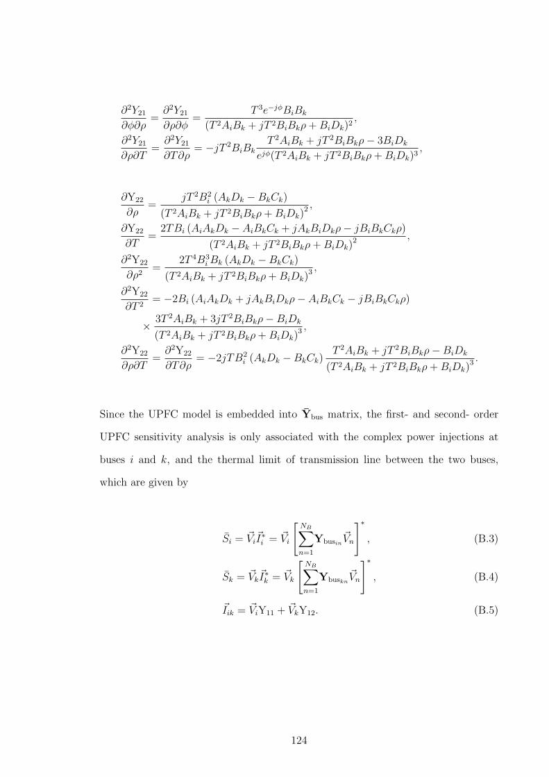
∂2Y21
∂φ∂ρ=
∂2Y21
∂ρ∂φ=
T 3e−jφBiBk
(T 2AiBk + jT 2BiBkρ + BiDk)2,
∂2Y21
∂ρ∂T=
∂2Y21
∂T∂ρ= −jT 2BiBk
T 2AiBk + jT 2BiBkρ− 3BiDk
ejφ(T 2AiBk + jT 2BiBkρ + BiDk)3,
∂Y22
∂ρ=
jT 2B2i (AkDk −BkCk)
(T 2AiBk + jT 2BiBkρ + BiDk)2 ,
∂Y22
∂T=
2TBi (AiAkDk − AiBkCk + jAkBiDkρ− jBiBkCkρ)
(T 2AiBk + jT 2BiBkρ + BiDk)2 ,
∂2Y22
∂ρ2=
2T 4B3i Bk (AkDk −BkCk)
(T 2AiBk + jT 2BiBkρ + BiDk)3 ,
∂2Y22
∂T 2= −2Bi (AiAkDk + jAkBiDkρ− AiBkCk − jBiBkCkρ)
× 3T 2AiBk + 3jT 2BiBkρ−BiDk
(T 2AiBk + jT 2BiBkρ + BiDk)3 ,
∂2Y22
∂ρ∂T=
∂2Y22
∂T∂ρ= −2jTB2
i (AkDk −BkCk)T 2AiBk + jT 2BiBkρ−BiDk
(T 2AiBk + jT 2BiBkρ + BiDk)3 .
Since the UPFC model is embedded into Ybus matrix, the first- and second- order
UPFC sensitivity analysis is only associated with the complex power injections at
buses i and k, and the thermal limit of transmission line between the two buses,
which are given by
Si = ~Vi~I∗i = ~Vi
[NB∑n=1
Ybusin~Vn
]∗, (B.3)
Sk = ~Vk~I∗k = ~Vk
[NB∑n=1
Ybuskn~Vn
]∗, (B.4)
~Iik = ~ViY11 + ~VkY12. (B.5)
124

Here, we assume that current flows from bus i to bus k. The first- and second-order
derivatives for the above equations are written as follows:
∂Si
∂φ= ~Vi
~V ∗k
(∂Y12
∂φ
)∗,
∂Sk
∂φ= ~Vk
~V ∗i
(∂Y21
∂φ
)∗,
∂Si
∂ρ= V 2
i
(∂Y11
∂ρ
)∗+ ~Vi
~V ∗k
(∂Y12
∂ρ
)∗,
∂Sk
∂ρ= ~Vk
~V ∗i
(∂Y21
∂ρ
)∗+ V 2
k
(∂Y22
∂ρ
)∗,
∂Si
∂T= V 2
i
(∂Y11
∂T
)∗+ ~Vi
~V ∗k
(∂Y12
∂T
)∗,
∂Sk
∂T= ~Vk
~V ∗i
(∂Y21
∂T
)∗+ V 2
k
(∂Y22
∂T
)∗,
∂~Iik
∂φ= ~Vk
∂Y12
∂φ,
∂~Iik
∂ρ= ~Vi
∂Y11
∂ρ+ ~Vk
∂Y12
∂ρ,
∂~Iik
∂T= ~Vi
∂Y11
∂T+ ~Vk
∂Y12
∂T,
∂~Iik
∂Vi
= ejθiY11,
∂~Iik
∂θi
= j~ViY11,
∂~Iik
∂Vk
= ejθkY12,
∂~Iik
∂θk
= j~VkY12,
∂~Iik~I∗ik
∂φ=
∂~Iik
∂φ~I∗ik +
∂~Iik
∂φ
∗~Iik,
∂~Iik~I∗ik
∂ρ=
∂~Iik
∂ρ~I∗ik +
∂~Iik
∂ρ
∗~Iik,
∂~Iik~I∗ik
∂T=
∂~Iik
∂T~I∗ik +
∂~Iik
∂T
∗~Iik,
∂2~Iik
∂φ2= ~Vk
∂2Y12
∂φ2,
125

∂2~Iik
∂ρ2=
(~Vi
∂2Y11
∂ρ2+ ~Vk
∂2Y12
∂ρ2
),
∂2~Iik
∂T 2=
(~Vi
∂2Y11
∂T 2+ ~Vk
∂2Y12
∂T 2
),
∂2~Iik
∂Vi∂ρ=
∂2~Iik
∂ρ∂Vi
= ejθi∂Y11
∂ρ,
∂2~Iik
∂Vi∂T=
∂2~Iik
∂T∂Vi
= ejθi∂Y11
∂T,
∂2~Iik
∂Vk∂φ=
∂2~Iik
∂φ∂Vk
= ejθk∂Y12
∂φ,
∂2~Iik
∂Vk∂ρ=
∂2~Iik
∂ρ∂Vk
= ejθk∂Y12
∂ρ,
∂2~Iik
∂Vk∂T=
∂2~Iik
∂T∂Vk
= ejθk∂Y12
∂T,
∂2~Iik
∂θi∂ρ=
∂2~Iik
∂ρ∂θi
= j~Vi∂Y11
∂ρ,
∂2~Iik
∂θi∂T=
∂2~Iik
∂T∂θi
= j~Vi∂Y11
∂T,
∂2~Iik
∂θk∂φ=
∂2~Iik
∂φ∂θk
= j~Vk∂Y12
∂φ,
∂2~Iik
∂θk∂ρ=
∂2~Iik
∂ρ∂θk
= j~Vk∂Y12
∂ρ,
∂2~Iik
∂θk∂T=
∂2~Iik
∂T∂θk
= j~Vk∂Y12
∂T,
∂2~Iik
∂φ∂ρ=
∂2~Iik
∂ρ∂φ= ~Vk
∂2Y12
∂φ∂ρ,
∂2~Iik
∂φ∂T=
∂2~Iik
∂T∂φ= ~Vk
∂2Y12
∂φ∂T,
∂2~Iik
∂ρ∂T=
∂2~Iik
∂T∂ρ= ~Vi
∂2Y11
∂ρ∂T+ ~Vk
∂2Y12
∂ρ∂T,
∂2Si
∂Vi∂φ=
∂2Si
∂φ∂Vi
= ejθi ~V ∗k
(∂Y12
∂φ
)∗,
∂2Si
∂θi∂φ=
∂2Si
∂φ∂θi
= j~Vi~V ∗
k
(∂Y12
∂φ
)∗,
∂2Si
∂Vk∂φ=
∂2Si
∂φ∂Vk
= ~Vie−jθk
(∂Y12
∂φ
)∗,
126
∂2Si
∂θk∂φ=
∂2Si
∂φ∂θk
= −j~Vi~V ∗
k
(∂Y12
∂φ
)∗,
∂2Si
∂Vi∂ρ=
∂2Si
∂ρ∂Vi
= 2Vi
(∂Y11
∂ρ
)∗+ ejθi ~V ∗
k
(∂Y12
∂ρ
)∗,
∂2Si
∂θi∂ρ=
∂2Si
∂ρ∂θi
= j~Vi~V ∗
k
(∂Y12
∂ρ
)∗,
∂2Si
∂Vk∂ρ=
∂2Si
∂ρ∂Vk
= ~Vie−jθk
(∂Y12
∂ρ
)∗,
∂2Si
∂θk∂ρ=
∂2Si
∂ρ∂θk
= −j~Vi~V ∗
k
(∂Y12
∂ρ
)∗,
∂2Si
∂Vi∂T=
∂2Si
∂T∂Vi
= 2Vi
(∂Y11
∂T
)∗+ ejθi ~V ∗
k
(∂Y12
∂T
)∗,
∂2Si
∂θi∂T=
∂2Si
∂T∂θi
= j~Vi~V ∗
k
(∂Y12
∂T
)∗,
∂2Si
∂Vk∂T=
∂2Si
∂T∂Vk
= ~Vie−jθk
(∂Y12
∂T
)∗,
∂2Si
∂θk∂T=
∂2Si
∂T∂θk
= −j~Vi~V ∗
k
(∂Y12
∂T
)∗,
∂2Si
∂φ2= ~Vi
~V ∗k
(∂2Y12
∂φ2
)∗,
∂2Si
∂ρ2= V 2
i
(∂2Y11
∂ρ2
)∗+ ~Vi
~V ∗k
(∂2Y12
∂ρ2
)∗,
∂2Si
∂T 2= V 2
i
(∂2Y11
∂T 2
)∗+ ~Vi
~V ∗k
(∂2Y12
∂T 2
)∗,
∂2Si
∂φ∂ρ=
∂2Si
∂ρ∂φ= ~Vi
~V ∗k
(∂2Y12
∂φ∂ρ
)∗,
∂2Si
∂φ∂T=
∂2Si
∂T∂φ= ~Vi
~V ∗k
(∂2Y12
∂φ∂T
)∗,
∂2Si
∂ρ∂T=
∂2Si
∂T∂ρ= V 2
i
(∂2Y11
∂ρ∂T
)∗+ ~Vi
~V ∗k
(∂2Y12
∂ρ∂T
)∗,
∂2Sk
∂Vi∂φ=
∂2Sk
∂φ∂Vi
= e−jθi ~Vk
(∂Y21
∂φ
)∗,
∂2Sk
∂θi∂φ=
∂2Sk
∂φ∂θi
= −j~V ∗i
~Vk
(∂Y21
∂φ
)∗,
127
∂2Sk
∂Vk∂φ=
∂2Sk
∂φ∂Vk
= ~V ∗i ejθk
(∂Y21
∂φ
)∗,
∂2Sk
∂θk∂φ=
∂2Sk
∂φ∂θk
= j~V ∗i
~Vk
(∂Y21
∂φ
)∗,
∂2Sk
∂Vi∂ρ=
∂2Sk
∂ρ∂Vi
= e−jθi ~Vk
(∂Y21
∂ρ
)∗,
∂2Sk
∂θi∂ρ=
∂2Sk
∂ρ∂θi
= −j~V ∗i
~Vk
(∂Y21
∂ρ
)∗,
∂2Sk
∂Vk∂ρ=
∂2Sk
∂ρ∂Vk
= ~V ∗i ejθk
(∂Y21
∂ρ
)∗+ 2Vk
(∂Y22
∂ρ
)∗,
∂2Sk
∂θk∂ρ=
∂2Sk
∂ρ∂θk
= j~V ∗i
~Vk
(∂Y21
∂ρ
)∗,
∂2Sk
∂Vi∂T=
∂2Sk
∂T∂Vi
= e−jθi ~Vk
(∂Y21
∂T
)∗,
∂2Sk
∂θi∂T=
∂2Sk
∂T∂θi
= −j~V ∗i
~Vk
(∂Y21
∂T
)∗,
∂2Sk
∂Vk∂T=
∂2Sk
∂T∂Vk
= ~V ∗i ejθk
(∂Y21
∂T
)∗+ 2Vk
(∂Y22
∂T
)∗,
∂2Sk
∂θk∂T=
∂2Sk
∂T∂θk
= j~V ∗i
~Vk
(∂Y21
∂T
)∗,
∂2Sk
∂φ2= ~V ∗
i~Vk
(∂2Y21
∂φ2
)∗,
∂2Sk
∂ρ2= ~V ∗
i~Vk
(∂2Y21
∂ρ2
)∗+ V 2
k
(∂2Y22
∂ρ2
)∗,
∂2Sk
∂T 2= ~V ∗
i~Vk
(∂2Y21
∂T 2
)∗+ V 2
k
(∂2Y22
∂T 2
)∗,
∂2Sk
∂φ∂ρ=
∂2Sk
∂ρ∂φ= ~V ∗
i~Vk
(∂2Y21
∂φ∂ρ
)∗,
∂2Sk
∂φ∂T=
∂2Sk
∂T∂φ= ~V ∗
i~Vk
(∂2Y21
∂φ∂T
)∗,
∂2Sk
∂ρ∂T=
∂2Sk
∂T∂ρ= ~V ∗
i~Vk
(∂2Y21
∂ρ∂T
)∗+ V 2
k
(∂2Y22
∂ρ∂T
)∗,
∂2~Iik~I∗ik
∂Vi∂φ=
∂2~Iik~I∗ik
∂φ∂Vi
= ~Iik∂2~I∗ik∂Vi∂φ
+∂~Iik
∂Vi
∂~I∗ik∂φ
+∂~I∗ik∂Vi
∂~Iik
∂φ+ ~I∗ik
∂2~Iik
∂Vi∂φ,
128
∂2~Iik~I∗ik
∂θi∂φ=
∂2~Iik~I∗ik
∂φ∂θi
= ~Iik∂2~I∗ik∂θi∂φ
+∂~Iik
∂θi
∂~I∗ik∂φ
+∂~I∗ik∂θi
∂~Iik
∂φ+ ~I∗ik
∂2~Iik
∂θi∂φ,
∂2~Iik~I∗ik
∂Vk∂φ=
∂2~Iik~I∗ik
∂φ∂Vk
= ~Iik∂2~I∗ik∂Vk∂φ
+∂~Iik
∂Vk
∂~I∗ik∂φ
+∂~I∗ik∂Vk
∂~Iik
∂φ+ ~I∗ik
∂2~Iik
∂Vk∂φ,
∂2~Iik~I∗ik
∂θk∂φ=
∂2~Iik~I∗ik
∂φ∂θk
= ~Iik∂2~I∗ik∂θk∂φ
+∂~Iik
∂θk
∂~I∗ik∂φ
+∂~I∗ik∂θk
∂~Iik
∂φ+ ~I∗ik
∂2~Iik
∂θk∂φ,
∂2~Iik~I∗ik
∂Vi∂ρ=
∂2~Iik~I∗ik
∂ρ∂Vi
= ~Iik∂2~I∗ik∂Vi∂ρ
+∂~Iik
∂Vi
∂~I∗ik∂ρ
+∂~I∗ik∂Vi
∂~Iik
∂ρ+ ~I∗ik
∂2~Iik
∂Vi∂ρ,
∂2~Iik~I∗ik
∂θi∂ρ=
∂2~Iik~I∗ik
∂ρ∂θi
= ~Iik∂2~I∗ik∂θi∂ρ
+∂~Iik
∂θi
∂~I∗ik∂ρ
+∂~I∗ik∂θi
∂~Iik
∂ρ+ ~I∗ik
∂2~Iik
∂θi∂ρ,
∂2~Iik~I∗ik
∂Vk∂ρ=
∂2~Iik~I∗ik
∂ρ∂Vk
= ~Iik∂2~I∗ik∂Vk∂ρ
+∂~Iik
∂Vk
∂~I∗ik∂ρ
+∂~I∗ik∂Vk
∂~Iik
∂ρ+ ~I∗ik
∂2~Iik
∂Vk∂ρ,
∂2~Iik~I∗ik
∂θk∂ρ=
∂2~Iik~I∗ik
∂ρ∂θk
= ~Iik∂2~I∗ik∂θk∂ρ
+∂~Iik
∂θk
∂~I∗ik∂ρ
+∂~I∗ik∂θk
∂~Iik
∂ρ+ ~I∗ik
∂2~Iik
∂θk∂ρ,
∂2~Iik~I∗ik
∂Vi∂T=
∂2~Iik~I∗ik
∂T∂Vi
= ~Iik∂2~I∗ik∂Vi∂T
+∂~Iik
∂Vi
∂~I∗ik∂T
+∂~I∗ik∂Vi
∂~Iik
∂T+ ~I∗ik
∂2~Iik
∂Vi∂T,
∂2~Iik~I∗ik
∂θi∂T=
∂2~Iik~I∗ik
∂T∂θi
= ~Iik∂2~I∗ik∂θi∂T
+∂~Iik
∂θi
∂~I∗ik∂T
+∂~I∗ik∂θi
∂~Iik
∂T+ ~I∗ik
∂2~Iik
∂θi∂T,
∂2~Iik~I∗ik
∂Vk∂T=
∂2~Iik~I∗ik
∂T∂Vk
= ~Iik∂2~I∗ik
∂Vk∂T+
∂~Iik
∂Vk
∂~I∗ik∂T
+∂~I∗ik∂Vk
∂~Iik
∂T+ ~I∗ik
∂2~Iik
∂Vk∂T,
∂2~Iik~I∗ik
∂θk∂T=
∂2~Iik~I∗ik
∂T∂θk
= ~Iik∂2~I∗ik
∂θk∂T+
∂~Iik
∂θk
∂~I∗ik∂T
+∂~I∗ik∂θk
∂~Iik
∂T+ ~I∗ik
∂2~Iik
∂θk∂T,
∂2~Iik~I∗ik
∂φ2= ~Iik
∂2~I∗ik∂φ2
+ 2∂~Iik
∂φ
∂~I∗ik∂φ
+ ~I∗ik∂2~Iik
∂φ2,
∂2~Iik~I∗ik
∂ρ2= ~Iik
∂2~I∗ik∂ρ2
+ 2∂~Iik
∂ρ
∂~I∗ik∂ρ
+ ~I∗ik∂2~Iik
∂ρ2,
∂2~Iik~I∗ik
∂T 2= ~Iik
∂2~I∗ik∂T 2
+ 2∂~Iik
∂T
∂~I∗ik∂T
+ ~I∗ik∂2~Iik
∂T 2,
∂2~Iik~I∗ik
∂φ∂ρ=
∂2~Iik~I∗ik
∂ρ∂φ= ~Iik
∂2~I∗ik∂φ∂ρ
+∂~Iik
∂φ
∂~I∗ik∂ρ
+∂~I∗ik∂φ
∂~Iik
∂ρ+ ~I∗ik
∂2~Iik
∂φ∂ρ,
∂2~Iik~I∗ik
∂φ∂T=
∂2~Iik~I∗ik
∂T∂φ= ~Iik
∂2~I∗ik∂φ∂T
+∂~Iik
∂φ
∂~I∗ik∂T
+∂~I∗ik∂φ
∂~Iik
∂T+ ~I∗ik
∂2~Iik
∂φ∂T,
∂2~Iik~I∗ik
∂ρ∂T=
∂2~Iik~I∗ik
∂T∂ρ= ~Iik
∂2~I∗ik∂ρ∂T
+∂~Iik
∂ρ
∂~I∗ik∂T
+∂~I∗ik∂ρ
∂~Iik
∂T+ ~I∗ik
∂2~Iik
∂ρ∂T,
129

APPENDIX C
INPUT DATA FILE FORMAT
The GEOPF program reads natural gas and electricity network data files. IEEE
Common Data Format (IEEE CDF) is used to obtain the electric transmission line
and bus input data [30]. We created Generation Data Format (GDF) and Load Data
Format (LDF) files for the electric network. In a similar way, we created Common
Gas Format (CGF) for the natural gas network.
C.1 IEEE Common Data Format
The data file has lines of up to 128 characters. The lines are grouped into sections
with section headers. Data items are entered in specific columns. No blank items are
allowed, enter zeros instead. Floating point items should have explicit decimal point.
No implicit decimal points are used. The IEEE CDF data which has been utilized in
the GEOPF program is described below:
130

¦ Title Data
Columns 2-9 Date, in format DD/MM/YY with leading zeros
11-30 Originator’s name
32-37 MVA base
39-42 Year
44 Season (S - Summer, W - Winter)
46-73 Case identification
¦ Bus Data
Columns 1-4 Bus number
7-17 Bus name
25-26 Type:
0=Unregulated (load, PQ)
1=Hold MVAR generation within voltage limits (PQ)
2=Hold voltage within VAR limits (PV)
3=Hold voltage and angle (Swing)
Columns 28-33 Bus voltage (loadflow result)
34-40 Bus angle (loadflow result)
41-49 Load MW (loadflow result)
50-59 Load MVAR (loadflow result)
60-67 Generation MW (loadflow result)
68-75 Generation MVAR (loadflow result)
91-98 Maximum voltage: for only bus type 0
99-106 Minimum voltage: for only bus type 0
107-114 Shunt conductance G (per unit)
115-122 Shunt susceptance B (per unit)
¦ Line Data
131

Columns 1-4 From bus
6-9 To bus
19 Line type:
1=Fixed voltage ratio and/or fixed phase shifter
2=Fixed phase angle and variable voltage ratio with
voltage control
3=Fixed phase angle and variable voltage ratio with
MVAR control
4=Fixed voltage ratio and variable phase shifter with
MW control
20-29 Branch resistance R, per unit
30-40 Branch reactance X, per unit
41-49 Line charging B, per unit
57-61 Maximum line flow (MVA): for emergency state
63-67 Maximum line flow (MVA): for normal operating state
77-82 Transformer tap ratio
84-90 Phase angle
91-97 Minimum limit of variable tap ratio or phase shifter
98-104 Maximum limit of variable tap ratio or phase shifter
132

C.2 Generator Data
Columns 1-5 Generator bus number
7-15 Generator name
17-23 Maximum real power generation
25-29 Minimum real power generation
31-38 Maximum reactive power generation
40-45 Minimum reactive power generation
40-45 Minimum reactive power generation
47 Adjustable real power generation:
0=real power generation is not adjustable
1=real power generation is adjustable
49 Adjustable reactive power generation:
0=reactive power generation is not adjustable
1=reactive power generation is adjustable
51 Availability:
0=the generator is not available
1=the generator is available
53-75 Generator cost function: αGi + βGiPGi + γGiP2Gi
53-59 αGi
61-66 βGi
68-75 γGi
77-81 Maximum voltage
83-87 Minimum voltage
133

C.3 Electricity Load Data
Columns 1-5 Load bus number
7-13 Load bus name
15-18 Load type:
1=residential
2=industrial
3=commercial
20-25 Maximum MW load
27-32 Minimum MW load
34-40 Maximum MVAR load
42-48 Minimum MVAR load
50 Interruptible load:
0=not interruptible
1=interruptable
52-59 Maximum MW interruptible
61-87 Customer benefit function: αLi + βLiPLi + γLiP2Li
53-59 αLi
61-66 βLi
68-75 γLi
77-81 Load power factor
134

C.4 Natural Gas Common Data Format
¦ Field Data
Columns 1-5 Standard temperature (◦R)
6-12 Standard pressure (psia)
14-19 Average gas compressibility factor
20-26 Compressor inlet compressibility factor
28-31 Gross heating value (BTU/SCF)
¦ Node Data
Columns 1-4 Node number
7-20 Node name
23 Type:
0=known-pressure node
1=load node (except combined node)
2=gas-electric combined node
3=compressor inlet node
4=compressor outlet node
29-37 Pressure, psia (loadflow result)
39-46 Supply, 106 × SCF/hr (loadflow result)
48-54 Load demand, 106 × SCF/hr (loadflow result)
56-60 Minimum pressure (psia)
62-66 Maximum pressure (psia)
¦ Pipeline Branch Data
135
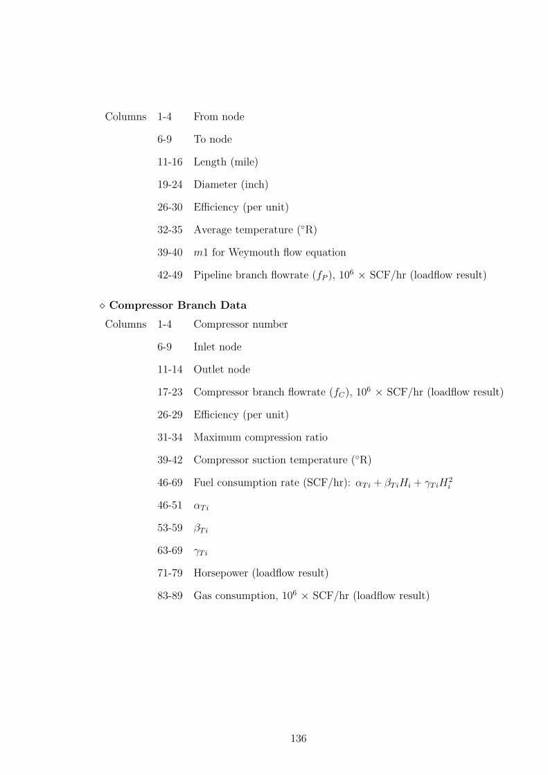
Columns 1-4 From node
6-9 To node
11-16 Length (mile)
19-24 Diameter (inch)
26-30 Efficiency (per unit)
32-35 Average temperature (◦R)
39-40 m1 for Weymouth flow equation
42-49 Pipeline branch flowrate (fP ), 106 × SCF/hr (loadflow result)
¦ Compressor Branch Data
Columns 1-4 Compressor number
6-9 Inlet node
11-14 Outlet node
17-23 Compressor branch flowrate (fC), 106 × SCF/hr (loadflow result)
26-29 Efficiency (per unit)
31-34 Maximum compression ratio
39-42 Compressor suction temperature (◦R)
46-69 Fuel consumption rate (SCF/hr): αTi + βTiHi + γTiH2i
46-51 αTi
53-59 βTi
63-69 γTi
71-79 Horsepower (loadflow result)
83-89 Gas consumption, 106 × SCF/hr (loadflow result)
136

C.5 Natural Gas Load Data
Columns 1-5 Node number
7-14 Node name
17 Load type:
1=residential
2=industrial
3=commercial
4=generator
20-22 Generator number if load is a generator.
24-27 Maximum load (106 × SCF/hr)
29-33 Minimum load (106 × SCF/hr)
37 Interruptible load:
0=not interruptible
1=interruptible
39-64 Consumer benefit function ($/hr): αLi + βLiwLi + γLiw2Li
39-44 αLi
47-54 βLi
57-64 γLi
137
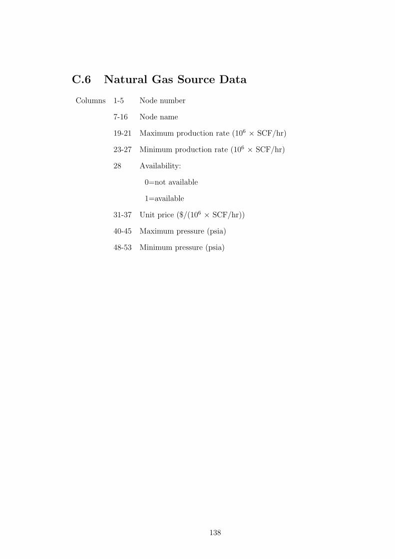
C.6 Natural Gas Source Data
Columns 1-5 Node number
7-16 Node name
19-21 Maximum production rate (106 × SCF/hr)
23-27 Minimum production rate (106 × SCF/hr)
28 Availability:
0=not available
1=available
31-37 Unit price ($/(106 × SCF/hr))
40-45 Maximum pressure (psia)
48-53 Minimum pressure (psia)
138
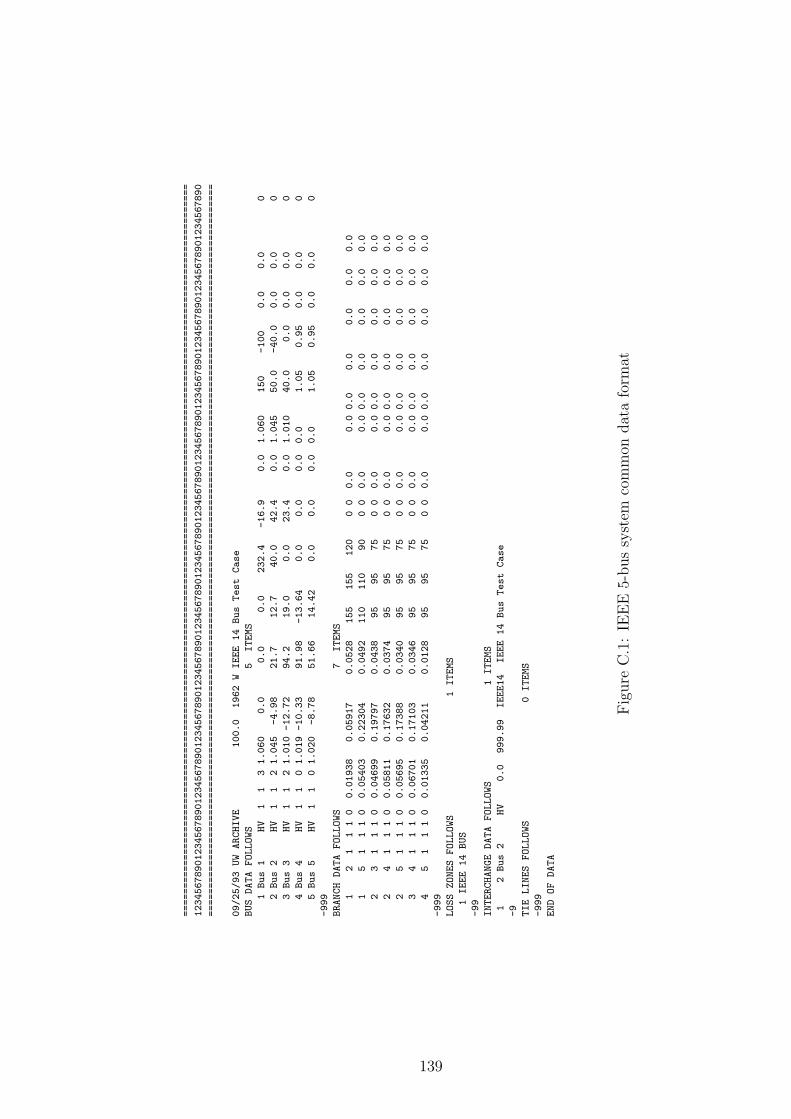
==================================================================================================================================
1234567890123456789012345678901234567890123456789012345678901234567890123456789012345678901234567890123456789012345678901234567890
==================================================================================================================================
09/25/93UW
ARCHIVE
100.0
1962
WIEEE
14
Bus
Test
Case
BUSDATA
FOLLOWS
5ITEMS
1Bus
1HV
11
31.060
0.0
0.0
0.0
232.4
-16.9
0.0
1.060
150
-100
0.0
0.0
0
2Bus
2HV
11
21.045
-4.98
21.7
12.7
40.0
42.4
0.0
1.045
50.0
-40.0
0.0
0.0
0
3Bus
3HV
11
21.010
-12.72
94.2
19.0
0.0
23.4
0.0
1.010
40.0
0.0
0.0
0.0
0
4Bus
4HV
11
01.019
-10.33
91.98
-13.64
0.0
0.0
0.0
0.0
1.05
0.95
0.0
0.0
0
5Bus
5HV
11
01.020
-8.78
51.66
14.42
0.0
0.0
0.0
0.0
1.05
0.95
0.0
0.0
0
-999
BRANCHDATA
FOLLOWS
7ITEMS
12
11
10
0.01938
0.05917
0.0528
155
155
120
00
0.0
0.0
0.0
0.0
0.0
0.0
0.0
15
11
10
0.05403
0.22304
0.0492
110
110
90
00
0.0
0.0
0.0
0.0
0.0
0.0
0.0
23
11
10
0.04699
0.19797
0.0438
95
95
75
00
0.0
0.0
0.0
0.0
0.0
0.0
0.0
24
11
10
0.05811
0.17632
0.0374
95
95
75
00
0.0
0.0
0.0
0.0
0.0
0.0
0.0
25
11
10
0.05695
0.17388
0.0340
95
95
75
00
0.0
0.0
0.0
0.0
0.0
0.0
0.0
34
11
10
0.06701
0.17103
0.0346
95
95
75
00
0.0
0.0
0.0
0.0
0.0
0.0
0.0
45
11
10
0.01335
0.04211
0.0128
95
95
75
00
0.0
0.0
0.0
0.0
0.0
0.0
0.0
-999
LOSSZONES
FOLLOWS
1ITEMS
1IEEE
14
BUS
-99
INTERCHANGEDATA
FOLLOWS
1ITEMS
12
Bus
2HV
0.0
999.99
IEEE14
IEEE
14
Bus
Test
Case
-9
TIELINES
FOLLOWS
0ITEMS
-999
ENDOF
DATA
Fig
ure
C.1
:IE
EE
5-bus
syst
emco
mm
ondat
afo
rmat
139

==================================================================================================================================
1234567890123456789012345678901234567890123456789012345678901234567890123456789012345678901234567890123456789012345678901234567890
==================================================================================================================================
BUNUM
GENERNAME
MX---MW
MN-MW
MX---MVR
MN-MVR
PQ
AAL__PHA
B-E-TA
GAM-M--A
V-MAX
V-MIN
MW-UP
MW-DN
MVARUP
MVARDN
BETA_R
GAMMAR
1GEN1
250.00
45.0
150.00
-100
11
1692.32
11.0
.000820
1.08
0.950
inf
inf
inf
inf
0.0
.00000
2GEN2
150.00
15.0
50.00
-40
11
1692.32
12.0
.000776
1.08
0.950
inf
inf
inf
inf
0.0
.00000
3SynCon
10.00
0.0
40.00
-40
01
10.0
0.0
.000000
1.08
0.950
inf
inf
inf
inf
0.0
.00000
Fig
ure
C.2
:IE
EE
5-bus
syst
emge
ner
ator
dat
afo
rmat
==================================================================================================================================
1234567890123456789012345678901234567890123456789012345678901234567890123456789012345678901234567890123456789012345678901234567890
==================================================================================================================================
BUNUM
BUSNAME
TYPE
MX--MW
MN--MW
MX-MVAR
MN-MVAR
RMX-MW-IN
ALPHA-LD
BETA--LD
GAMMA--LD
ALPHA-IN
BETA-IN
GAMMA-IN
P----F
2Residen
1inf
0.0
inf
-inf
1inf
0.00
21.43
-0.2147
0.0
100.0
0.0
0.98
3Indust1
2inf
0.0
inf
-inf
1inf
0.00
23.00
-0.0531
0.0
100.0
0.0
0.98
4Indust2
2inf
0.0
inf
-inf
1inf
0.00
22.48
-0.0531
0.0
100.0
0.0
0.98
5Commerc
3inf
0.0
inf
-inf
1inf
0.00
22.11
-0.0930
0.0
100.0
0.0
0.98
Fig
ure
C.3
:IE
EE
5-bus
syst
emlo
addat
afo
rmat
140

07/20/94OSU
mods
to
UW
case
100.0
1962
WIEEE14
W/LINE
LIMITS,
BUS
KV
BUSDATA
FOLLOWS
14
ITEMS
1Bus
1HV
11
31.0600
.00
.00
.00
232.39
-16.90
230.00
1.0600
150.00
-100.00
.0000
.0000
0
2Bus
2HV
11
21.0450
-4.98
21.70
12.70
40.00
42.41
230.00
1.0450
50.00
-40.00
.0000
.0000
0
3Bus
3HV
11
21.0100
-12.72
94.20
19.00
.00
23.39
230.00
1.0100
40.00
.00
.0000
.0000
0
4Bus
4HV
11
01.0186
-10.32
47.80
-3.90
.00
.00
230.00
.0000
1.05
0.950
.0000
.0000
0
5Bus
5HV
11
01.0203
-8.78
7.60
1.60
.00
.00
230.00
.0000
1.05
0.950
.0000
.0000
0
6Bus
6LV
11
21.0700
-14.22
11.20
7.50
.00
12.24
69.00
1.0700
24.00
-6.00
.0000
.0000
0
7Bus
7ZV
11
01.0620
-13.37
.00
.00
.00
.00
161.00
.0000
1.250
0.750
.0000
.0000
0
8Bus
8TV
11
21.0900
-13.37
.00
.00
.00
17.36
138.00
1.0900
24.00
-6.00
.0000
.0000
0
9Bus
9LV
11
01.0563
-14.95
29.50
16.60
.00
.00
69.00
.0000
1.050
0.950
.0000
.1900
0
10
Bus
10
LV
11
01.0513
-15.10
9.00
5.80
.00
.00
69.00
.0000
1.050
0.950
.0000
.0000
0
11
Bus
11
LV
11
01.0571
-14.80
3.50
1.80
.00
.00
69.00
.0000
1.050
0.900
.0000
.0000
0
12
Bus
12
LV
11
01.0552
-15.08
6.10
1.60
.00
.00
69.00
.0000
1.050
0.950
.0000
.0000
0
13
Bus
13
LV
11
01.0504
-15.16
13.50
5.80
.00
.00
69.00
.0000
1.050
0.950
.0000
.0000
0
14
Bus
14
LV
11
01.0358
-16.04
14.90
5.00
.00
.00
69.00
.0000
1.050
0.950
.0000
.0000
0
-999
BRANCHDATA
FOLLOWS
20
ITEMS
12
11
10
.019380
.059170
.05280
175.
175.
120.
00
.0000
.00
.0000
.0000
.00000
.0000
.0000
15
11
10
.054030
.223040
.04920
90.
90.
90.
00
.0000
.00
.0000
.0000
.00000
.0000
.0000
23
11
10
.046990
.197970
.04380
75.
75.
75.
00
.0000
.00
.0000
.0000
.00000
.0000
.0000
24
11
10
.058110
.176320
.03740
75.
75.
75.
00
.0000
.00
.0000
.0000
.00000
.0000
.0000
25
11
10
.056950
.173880
.03400
50.
50.
50.
00
.0000
.00
.0000
.0000
.00000
.0000
.0000
34
11
10
.067010
.171030
.03460
50.
50.
50.
00
.0000
.00
.0000
.0000
.00000
.0000
.0000
45
11
10
.013350
.042110
.01280
90.
90.
90.
00
.0000
.00
.0000
.0000
.00000
.0000
.0000
611
11
10
.094980
.198900
.00000
10.
10.
10.
00
.0000
.00
.0000
.0000
.00000
.0000
.0000
612
11
10
.122910
.255810
.00000
10.
10.
10.
00
.0000
.00
.0000
.0000
.00000
.0000
.0000
613
11
10
.066150
.130270
.00000
20.
20.
20.
00
.0000
.00
.0000
.0000
.00000
.0000
.0000
910
11
10
.031810
.084500
.00000
10.
10.
10.
00
.0000
.00
.0000
.0000
.00000
.0000
.0000
914
11
10
.127110
.270380
.00000
15.
15.
15.
00
.0000
.00
.0000
.0000
.00000
.0000
.0000
10
11
11
10
.082050
.192070
.00000
10.
10.
10.
00
.0000
.00
.0000
.0000
.00000
.0000
.0000
12
13
11
10
.220920
.199880
.00000
10.
10.
10.
00
.0000
.00
.0000
.0000
.00000
.0000
.0000
13
14
11
10
.170930
.348020
.00000
10.
10.
10.
00
.0000
.00
.0000
.0000
.00000
.0000
.0000
47
11
11
.000000
.209120
.00000
35.
35.
35.
00
.9780
.00
.0000
.0000
.00000
.0000
.0000
49
11
11
.000000
.556180
.00000
20.
20.
20.
00
.9690
.00
.0000
.0000
.00000
.0000
.0000
56
11
11
.000000
.252020
.00000
50.
50.
50.
00
.9320
.00
.0000
.0000
.00000
.0000
.0000
78
11
11
.000000
.176150
.00000
20.
20.
20.
00
1.0000
.00
.0000
.0000
.00000
.0000
.0000
79
11
11
.000000
.110010
.00000
35.
35.
35.
00
1.0000
.00
.0000
.0000
.00000
.0000
.0000
-999
Fig
ure
C.4
:IE
EE
14-b
us
syst
emco
mm
ondat
afo
rmat
141

==================================================================================================================================
1234567890123456789012345678901234567890123456789012345678901234567890123456789012345678901234567890123456789012345678901234567890
==================================================================================================================================
BUNUM
GENERNAME
MX--GEN
MNGEN
MX---MVR
MN-MVR
PQ
AAL--PHA
B-E-TA
GAM---MA
V-MAX
V-MIN
MW-UP
MW-DN
MVARUP
MVARDN
BETA-R
GAMMAR
1GEN
1250.00
45.0
150.00
-100
11
1692.32
11.0
.000820
1.080
0.950
inf
inf
inf
inf
0.0
.00000
2GEN
2150.00
15.0
50.00
-40
11
1692.32
12.0
.000776
1.080
0.950
inf
inf
inf
inf
0.0
.00000
3SynCon
10.00
0.00
40.00
00
11
0.00
0.0
.000000
1.080
0.950
inf
inf
inf
inf
0.0
.00000
6SynCon
20.00
0.00
54.00
-50
01
10.00
0.0
.000000
1.080
0.950
inf
inf
inf
inf
0.0
.00000
8SynCon
30.00
0.00
54.00
-50
01
10.00
0.0
.000000
1.080
0.950
inf
inf
inf
inf
0.0
.00000
Fig
ure
C.5
:IE
EE
14-b
us
syst
emge
ner
ator
dat
afo
rmat
==================================================================================================================================
1234567890123456789012345678901234567890123456789012345678901234567890123456789012345678901234567890123456789012345678901234567890
==================================================================================================================================
BUNUM
BUSNAME
TYPE
MX--MW
MN--MW
MX-MVAR
MN-MVAR
RMX-MW-IN
ALPHA-LD
BETA--LD
GAMMA--LD
ALPHA-IN
BETA-IN
GAMMA-IN
P----F
2Residen
1inf
0.0
inf
-inf
1inf
0.00
21.43
-0.2146
0.0
100.0
0.0
0.98
3Indust1
2inf
0.0
inf
-inf
1inf
0.00
22.98
-0.0530
0.0
100.0
0.0
0.98
4Indust2
2inf
0.0
inf
-inf
1inf
0.00
22.45
-0.1021
0.0
100.0
0.0
0.98
5Commerc
3inf
0.0
inf
-inf
1inf
0.00
22.07
-0.6314
0.0
100.0
0.0
0.98
6Residen
1inf
0.0
inf
-inf
1inf
0.00
22.11
-0.4292
0.0
100.0
0.0
0.98
9Residen
1inf
0.0
inf
-inf
1inf
0.00
22.41
-0.1652
0.0
100.0
0.0
0.98
10Residen
1inf
0.0
inf
-inf
1inf
0.00
22.50
-0.5434
0.0
100.0
0.0
0.98
11Residen
1inf
0.0
inf
-inf
1inf
0.00
22.39
-1.3904
0.0
100.0
0.0
0.98
12Residen
1inf
0.0
inf
-inf
1inf
0.00
22.51
-0.8022
0.0
100.0
0.0
0.98
13Residen
1inf
0.0
inf
-inf
1inf
0.00
22.63
-0.3644
0.0
100.0
0.0
0.98
14Residen
1inf
0.0
inf
-inf
1inf
0.00
23.02
-0.3359
0.0
100.0
0.0
0.98
Fig
ure
C.6
:IE
EE
14-b
us
syst
emlo
addat
afo
rmat
142

==================================================================================================================================
1234567890123456789012345678901234567890123456789012345678901234567890123456789012345678901234567890123456789012345678901234567890
==================================================================================================================================
07/20/94
OSU
mods
to
UW
case
100.0
1962
WIEEE14
W/LINE
LIMITS,
BUS
KV
BUS
DATA
FOLLOWS
9ITEMS
1Bus
1HV
11
31.0300
.00
.00
.00
72.000
30.00
230.00
1.0600
150.00
-100.00
.0000
.0000
0
2Bus
2HV
11
21.0250
8.98
0.000
0.00
163.00
6.41
230.00
1.0450
50.00
-40.00
.0000
.0000
0
3Bus
3HV
11
21.0250
5.72
0.00
0.00
85.00
-11.9
230.00
1.0100
40.00
.00
.0000
.0000
0
4Bus
4HV
11
01.0256
-2.32
0.0
0.00
.00
.00
230.00
.0000
1.05
0.955
.0000
.0000
0
5Bus
5HV
11
00.9900
-4.78
125.0
50.00
.00
.00
230.00
.0000
1.05
0.955
.0000
.0000
0
6Bus
6LV
11
01.0100
-4.22
90.0
30.00
.00
.00
69.00
1.0700
1.050
0.955
.0000
.0000
0
7Bus
7ZV
11
01.0220
3.37
.00
.00
.00
.00
161.00
.0000
1.050
0.955
.0000
.0000
0
8Bus
8TV
11
01.0100
0.37
100.0
35.00
.00
.00
138.00
1.0900
1.050
0.950
.0000
.0000
0
9Bus
9LV
11
01.0363
2.95
0.00
0.00
.00
.00
69.00
.0000
1.050
0.955
.0000
.1900
0
-999
BRANCH
DATA
FOLLOWS
9ITEMS
46
11
10
.017000
.092000
.15800
120.
155.
320.
00
.0000
.00
.0000
.0000
.00000
.0000
45
11
10
.010000
.085000
.17600
90.
110.
390.
00
.0000
.00
.0000
.0000
.00000
.0000
57
11
10
.032000
.161000
.30600
75.
95.
375.
00
.0000
.00
.0000
.0000
.00000
.0000
69
11
10
.039000
.170000
.35800
75.
95.
375.
00
.0000
.00
.0000
.0000
.00000
.0000
78
11
10
.008500
.072000
.14900
50.
95.
350.
00
.0000
.00
.0000
.0000
.00000
.0000
98
11
10
.011900
.100800
.20900
50.
95.
350.
00
.0000
.00
.0000
.0000
.00000
.0000
14
11
11
.000000
.057600
.00000
50.
60.
450.
00
.9320
.00
.0000
.0000
.00000
.0000
27
11
11
.000000
.062500
.00000
20.
30.
320.
00
1.0000
.00
.0000
.0000
.00000
.0000
39
11
11
.000000
.058600
.00000
35.
45.
335.
00
1.0000
.00
.0000
.0000
.00000
.0000
-999
LOSS
ZONES
FOLLOWS
1ITEMS
1IEEE
14
BUS
-99
INTERCHANGE
DATA
FOLLOWS
1ITEMS
12
Bus
2HV
.0
999.99
IEEE14
IEEE
14
Bus
Test
Case
-9
TIE
LINES
FOLLOW
0ITEMS
-999
END
OF
DATA
Fig
ure
C.7
:W
SC
C9-
bus
syst
emco
mm
ondat
afo
rmat
143

==================================================================================================================================
1234567890123456789012345678901234567890123456789012345678901234567890123456789012345678901234567890123456789012345678901234567890
==================================================================================================================================
BUNUM
GENERNAME
MX---MW
MN-MW
MX---MVR
MN-MVR
PQ
AAL__PHA
B-E-TA
GAM-M--A
V-MAX
V-MIN
MW-UP
MW-DN
MVARUP
MVARDN
BETA_R
GAMMAR
1GEN1
250.00
21.6
150.00
-100
11
10.0
12.712
.000820
1.040
0.950
50.0
50.0
inf
inf
0.0
.00000
2GEN2
271.64
25.0
50.00
-40
11
10.0
12.001
.000876
1.045
0.955
35.0
35.0
inf
inf
0.0
.00000
3GEN3
285.00
25.0
50.00
-40
11
10.0
12.290
.000646
1.045
0.955
35.0
35.0
inf
inf
0.0
.00000
Fig
ure
C.8
:W
SC
C9-
bus
syst
emge
ner
ator
dat
afo
rmat
==================================================================================================================================
1234567890123456789012345678901234567890123456789012345678901234567890123456789012345678901234567890123456789012345678901234567890
==================================================================================================================================
BUNUM
BUSNAME
TYPE
MX--MW
MN--MW
MX-MVAR
MN-MVAR
RMX-MW-IN
ALPHA-LD
BETA--LD
GAMMA--LD
ALPHA-IN
BETA-IN
GAMMA-IN
P----F
5Residen
1125.1
0.00
inf
-inf
1inf
0.00
38.6650
-.1047
0.0
100.0
0.0
0.9285
6Indust1
290.1
0.00
inf
-inf
1inf
0.00
16.8440
-.0231
0.0
100.0
0.0
0.9487
8Indust2
2100.1
0.00
inf
-inf
1inf
0.00
21.6300
-.0431
0.0
100.0
0.0
0.9439
Fig
ure
C.9
:W
SC
C9-
bus
syst
emlo
addat
afo
rmat
144

==========================================================================================
012345678901234567890123456789012345678901234567890123456789012345678901234567890123456789
==========================================================================================
10/26/02 OSU ARCHIVE 1000000.0 GEOPF 15 Node Case
FIELD CONDITION
520 14.65 0.9 0.955 1015
NODE DATA FOLLOWS 15 ITEMS
1 Node 1 HP 0 1000.000 7.288 0.000 600 1200
2 Node 2 HP 0 978.630 6.867 0.000 600 1200
3 Node 3 HP 1 729.716 0.000 3.838 500 1200
4 Node 4 HP 2 737.345 0.000 1.218 500 1200
5 Node 5 HP 3 575.481 0.000 0.000 400 1200
6 Node 6 HP 4 1035.000 0.000 0.000 400 1200
7 Node 7 HP 3 607.588 0.000 0.000 400 1200
8 Node 8 HP 4 1154.400 0.000 0.000 400 1200
9 Node 9 HP 3 918.628 0.000 0.000 400 1200
10 Node 10 HP 4 951.000 0.000 0.000 400 1200
11 Node 11 HP 3 932.810 0.000 0.000 400 1200
12 Node 12 HP 4 932.810 0.000 0.000 400 1200
13 Node 13 HP 1 601.554 0.000 4.263 600 1000
14 Node 14 HP 1 600.778 0.000 4.274 600 1000
15 Node 15 HP 2 600.000 0.000 0.501 600 1000
-999
BRANCH DATA FOLLOWS 12 ITEMS
1 3 80.5 19.56 0.90 520 2 7.2883
2 4 80.3 19.56 0.90 520 2 6.8673
3 4 55.9 19.56 0.90 520 2 -1.3533
3 5 81.1 19.62 0.90 520 2 4.8039
4 7 87.9 19.62 0.90 520 2 4.2963
6 9 93.5 19.62 0.90 520 2 4.7733
8 11 99.7 16.69 0.90 520 2 4.2667
10 13 93.5 16.69 0.90 520 2 4.7716
12 14 97.9 16.69 0.85 520 2 4.2667
13 14 86.6 16.69 0.90 520 2 0.2056
13 15 79.7 16.69 0.90 520 2 0.3032
14 15 83.5 16.69 0.85 520 2 0.1979
-999
COMPRESSOR STATION DATA FOLLOWS 4 ITEMS
1 5 6 4.4060 0.83 1.8 520 0.0000 8.3300 0.00000 3667.292 0.0305
2 7 8 4.2088 0.84 1.9 520 0.0000 8.3300 0.00000 3558.156 0.0296
3 9 10 4.4060 0.83 1.8 520 0.0000 8.3300 0.00000 203.203 0.0017
4 11 12 4.2088 0.84 1.9 520 0.0000 8.3300 0.00000 0.000 0.0000
-999
BENEFIT DATA FOLLOWS 5 ITEMS
3 Load 1 1 0 80 0.0 1 0.0 5980.0 -499.344
4 Load 2 4 2 90 0.0 0 0.0 5844.8 -460.944
13 Load 3 2 0 90 0.0 1 0.0 5980.0 -443.520
14 Load 4 3 0 90 0.0 1 0.0 5571.8 -394.560
15 Load 5 4 3 30 0.0 0 0.0 5748.6 -496.800
-999
SOURCE DATA FOLLOWS 2 ITEMS
1 Source 1 200 0.0 1 2550.0 1000.0 600.0
2 Source 2 200 0.0 1 2550.0 1000.0 600.0
-999
END OF DATA
Figure C.10: 15-node natural gas data format
145

APPENDIX D
MATLAB CODE
D.1 GEOPF% ==================== Gas and Electricity Optimal Power Flow ==================
% This program returns the solution of the natural gas and electricity optimal
% power flow (GEOPF).
% ==============================================================================
format compact;
clear all;
nu = 10;
psi =0.1;
% ------------------------------------------------------------------------------
% Read gas data file
Filename = input(’Gas Network Case Name: ’,’s’);
f.cgffile = [ Filename ’.cgf’ ];
a = ReadGasDF(f);
x = GasDataCon(a);
% ------------------------------------------------------------------------------
% Field Condition
base = x.base; % base unit
To = x.To; % standard temperature, oR
po = x.po; % standard pressure, psia
Za = x.Za; % average gas compressibility factor
Zi = x.Zi; % compressor inlet compressibility factor
G = x.G; % gas specific gravity
GHV = x.GHV; % gross heating value (BTU/ft^3}
CpCv = x.CpCv; % specific heat ratio
m1 = x.m1; % flow equation coefficient
% End of field condition
% ------------------------------------------------------------------------------
% Node Data
NN = x.NN; % # of nodes
loadNode = x.loadNode; % load nodes
combGasNode = x.combGasNode; % gas-electric combined nodes
NGE = x.NGE; % # of gas-elec. combined nodes
GE_load_no = x.GEloadNo; % gas-electric combined load #
NL = x.NL; % # of load nodes
sourceNode = x.sourceNode; % source nodes
refNode = x.sourceNode(1); % ref node
NS = x.NS; % # of source node
Pini = x.Pini; % initial node pressure
Wsrcini = x.Wsrcini; % initial gas supply
Wloadini = x.Wloadini; % initial gas consumption
Pref = x.Pref; % source node pressure
Pmin = x.Pmin; % min. nodal pressure
Pmax = x.Pmax; % max. nodal pressure
N = x.N; % nodal-gas injection incidence matrix
146
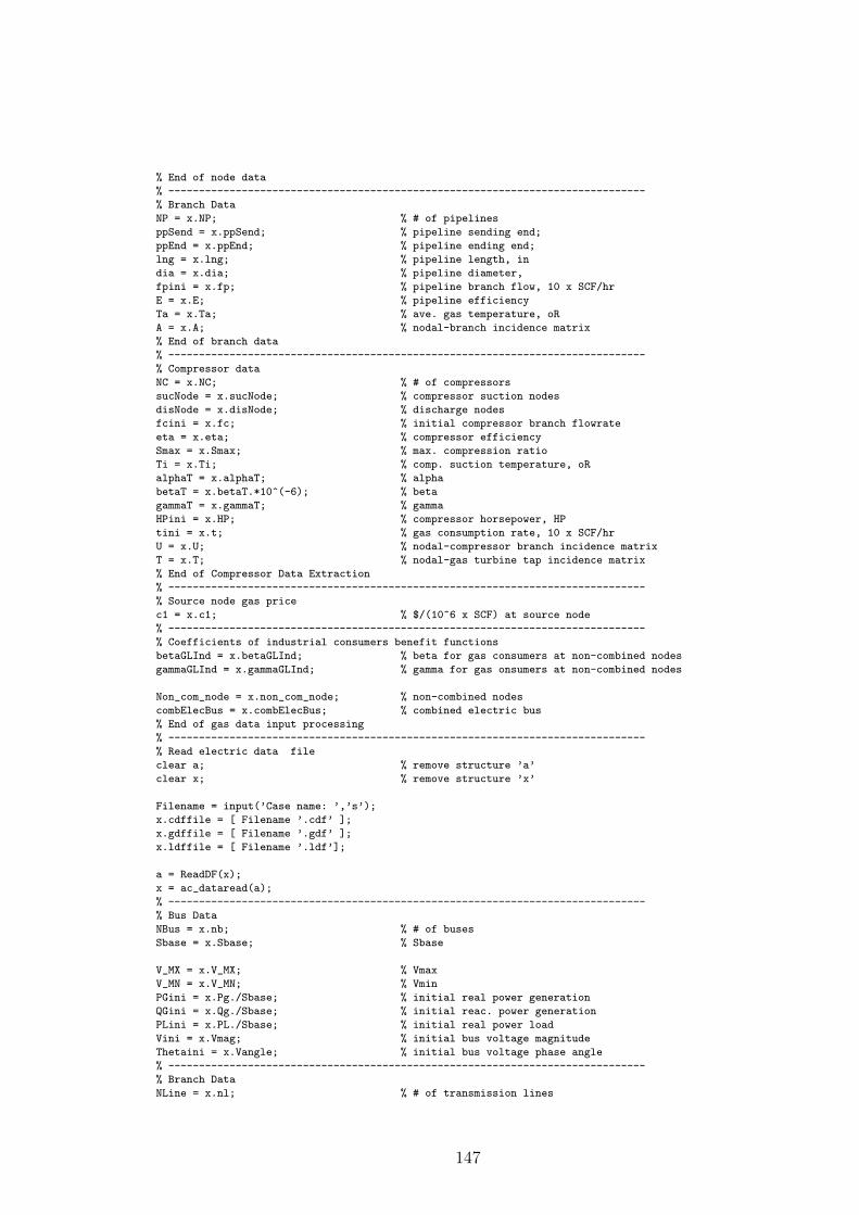
% End of node data
% ------------------------------------------------------------------------------
% Branch Data
NP = x.NP; % # of pipelines
ppSend = x.ppSend; % pipeline sending end;
ppEnd = x.ppEnd; % pipeline ending end;
lng = x.lng; % pipeline length, in
dia = x.dia; % pipeline diameter,
fpini = x.fp; % pipeline branch flow, 10 x SCF/hr
E = x.E; % pipeline efficiency
Ta = x.Ta; % ave. gas temperature, oR
A = x.A; % nodal-branch incidence matrix
% End of branch data
% ------------------------------------------------------------------------------
% Compressor data
NC = x.NC; % # of compressors
sucNode = x.sucNode; % compressor suction nodes
disNode = x.disNode; % discharge nodes
fcini = x.fc; % initial compressor branch flowrate
eta = x.eta; % compressor efficiency
Smax = x.Smax; % max. compression ratio
Ti = x.Ti; % comp. suction temperature, oR
alphaT = x.alphaT; % alpha
betaT = x.betaT.*10^(-6); % beta
gammaT = x.gammaT; % gamma
HPini = x.HP; % compressor horsepower, HP
tini = x.t; % gas consumption rate, 10 x SCF/hr
U = x.U; % nodal-compressor branch incidence matrix
T = x.T; % nodal-gas turbine tap incidence matrix
% End of Compressor Data Extraction
% ------------------------------------------------------------------------------
% Source node gas price
c1 = x.c1; % $/(10^6 x SCF) at source node
% ------------------------------------------------------------------------------
% Coefficients of industrial consumers benefit functions
betaGLInd = x.betaGLInd; % beta for gas consumers at non-combined nodes
gammaGLInd = x.gammaGLInd; % gamma for gas onsumers at non-combined nodes
Non_com_node = x.non_com_node; % non-combined nodes
combElecBus = x.combElecBus; % combined electric bus
% End of gas data input processing
% ------------------------------------------------------------------------------
% Read electric data file
clear a; % remove structure ’a’
clear x; % remove structure ’x’
Filename = input(’Case name: ’,’s’);
x.cdffile = [ Filename ’.cdf’ ];
x.gdffile = [ Filename ’.gdf’ ];
x.ldffile = [ Filename ’.ldf’];
a = ReadDF(x);
x = ac_dataread(a);
% ------------------------------------------------------------------------------
% Bus Data
NBus = x.nb; % # of buses
Sbase = x.Sbase; % Sbase
V_MX = x.V_MX; % Vmax
V_MN = x.V_MN; % Vmin
PGini = x.Pg./Sbase; % initial real power generation
QGini = x.Qg./Sbase; % initial reac. power generation
PLini = x.PL./Sbase; % initial real power load
Vini = x.Vmag; % initial bus voltage magnitude
Thetaini = x.Vangle; % initial bus voltage phase angle
% ------------------------------------------------------------------------------
% Branch Data
NLine = x.nl; % # of transmission lines
147
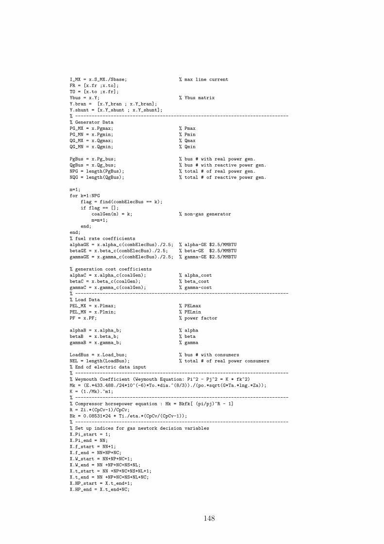
I_MX = x.S_MX./Sbase; % max line current
FR = [x.fr ;x.to];
TO = [x.to ;x.fr];
Ybus = x.Y; % Ybus matrix
Y.bran = [x.Y_bran ; x.Y_bran];
Y.shunt = [x.Y_shunt ; x.Y_shunt];
% ------------------------------------------------------------------------------
% Generator Data
PG_MX = x.Pgmax; % Pmax
PG_MN = x.Pgmin; % Pmin
QG_MX = x.Qgmax; % Qmax
QG_MN = x.Qgmin; % Qmin
PgBus = x.Pg_bus; % bus # with real power gen.
QgBus = x.Qg_bus; % bus # with reactive power gen.
NPG = length(PgBus); % total # of real power gen.
NQG = length(QgBus); % total # of reactive power gen.
m=1;
for k=1:NPG
flag = find(combElecBus == k);
if flag == [];
coalGen(m) = k; % non-gas generator
m=m+1;
end;
end;
% fuel rate coefficients
alphaGE = x.alpha_c(combElecBus)./2.5; % alpha-GE $2.5/MMBTU
betaGE = x.beta_c(combElecBus)./2.5; % beta-GE $2.5/MMBTU
gammaGE = x.gamma_c(combElecBus)./2.5; % gamma-GE $2.5/MMBTU
% generation cost coefficients
alphaC = x.alpha_c(coalGen); % alpha_cost
betaC = x.beta_c(coalGen); % beta_cost
gammaC = x.gamma_c(coalGen); % gamma-cost
% ------------------------------------------------------------------------------
% Load Data
PEL_MX = x.Plmax; % PELmax
PEL_MN = x.Plmin; % PELmin
PF = x.PF; % power factor
alphaB = x.alpha_b; % alpha
betaB = x.beta_b; % beta
gammaB = x.gamma_b; % gamma
LoadBus = x.Load_bus; % bus # with consumers
NEL = length(LoadBus); % total # of real power consumers
% End of electric data input
% ------------------------------------------------------------------------------
% Weymouth Coefficient (Weymouth Equation: Pi^2 - Pj^2 = K * fk^2)
Mk = (E.*433.488./24*10^(-6)*To.*dia.^(8/3))./(po.*sqrt(G*Ta.*lng.*Za));
K = (1./Mk).^m1;
% ------------------------------------------------------------------------------
% Compressor horsepower equation : Hk = Bkfk[ (pi/pj)^R - 1]
R = Zi.*(CpCv-1)/CpCv;
Bk = 0.08531*24 * Ti./eta.*(CpCv/(CpCv-1));
% ------------------------------------------------------------------------------
% Set up indices for gas newtork decision variables
X.Pi_start = 1;
X.Pi_end = NN;
X.f_start = NN+1;
X.f_end = NN+NP+NC;
X.W_start = NN+NP+NC+1;
X.W_end = NN +NP+NC+NS+NL;
X.t_start = NN +NP+NC+NS+NL+1;
X.t_end = NN +NP+NC+NS+NL+NC;
X.HP_start = X.t_end+1;
X.HP_end = X.t_end+NC;
148
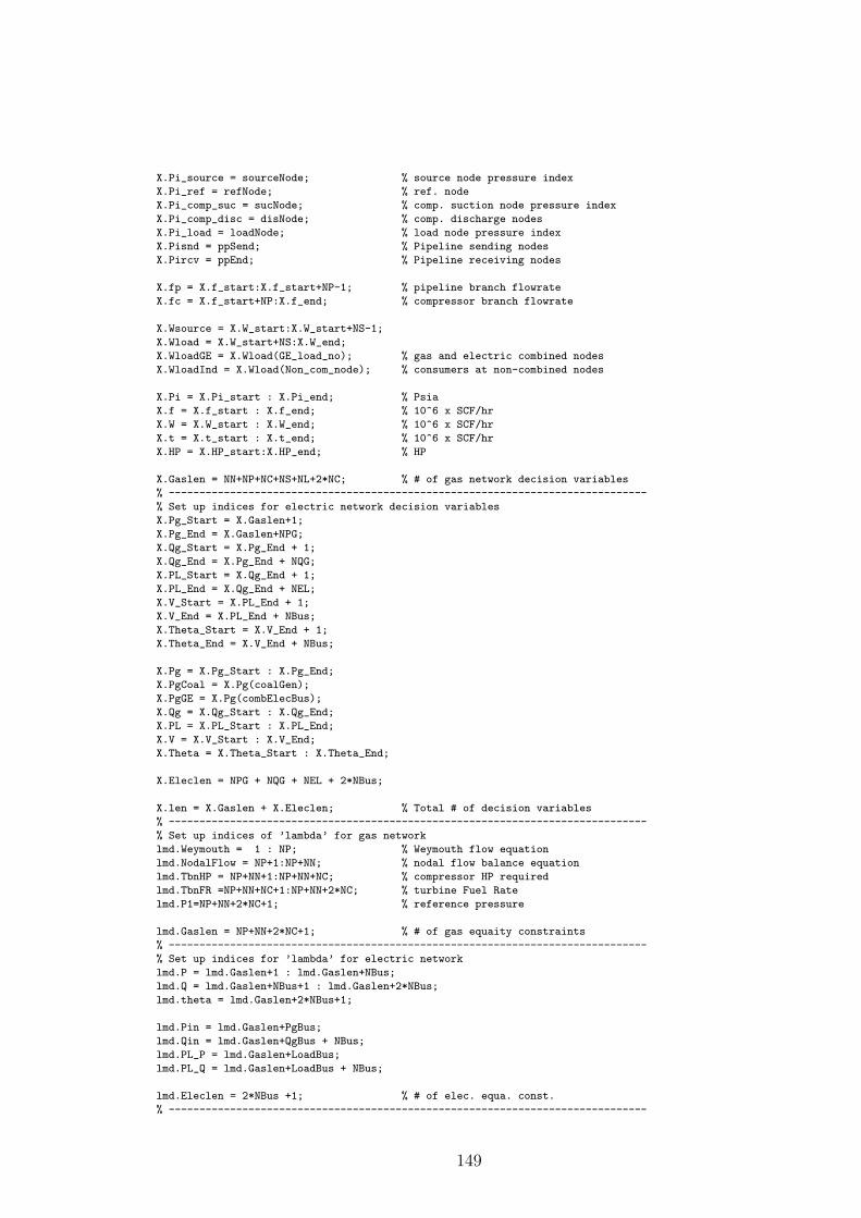
X.Pi_source = sourceNode; % source node pressure index
X.Pi_ref = refNode; % ref. node
X.Pi_comp_suc = sucNode; % comp. suction node pressure index
X.Pi_comp_disc = disNode; % comp. discharge nodes
X.Pi_load = loadNode; % load node pressure index
X.Pisnd = ppSend; % Pipeline sending nodes
X.Pircv = ppEnd; % Pipeline receiving nodes
X.fp = X.f_start:X.f_start+NP-1; % pipeline branch flowrate
X.fc = X.f_start+NP:X.f_end; % compressor branch flowrate
X.Wsource = X.W_start:X.W_start+NS-1;
X.Wload = X.W_start+NS:X.W_end;
X.WloadGE = X.Wload(GE_load_no); % gas and electric combined nodes
X.WloadInd = X.Wload(Non_com_node); % consumers at non-combined nodes
X.Pi = X.Pi_start : X.Pi_end; % Psia
X.f = X.f_start : X.f_end; % 10^6 x SCF/hr
X.W = X.W_start : X.W_end; % 10^6 x SCF/hr
X.t = X.t_start : X.t_end; % 10^6 x SCF/hr
X.HP = X.HP_start:X.HP_end; % HP
X.Gaslen = NN+NP+NC+NS+NL+2*NC; % # of gas network decision variables
% ------------------------------------------------------------------------------
% Set up indices for electric network decision variables
X.Pg_Start = X.Gaslen+1;
X.Pg_End = X.Gaslen+NPG;
X.Qg_Start = X.Pg_End + 1;
X.Qg_End = X.Pg_End + NQG;
X.PL_Start = X.Qg_End + 1;
X.PL_End = X.Qg_End + NEL;
X.V_Start = X.PL_End + 1;
X.V_End = X.PL_End + NBus;
X.Theta_Start = X.V_End + 1;
X.Theta_End = X.V_End + NBus;
X.Pg = X.Pg_Start : X.Pg_End;
X.PgCoal = X.Pg(coalGen);
X.PgGE = X.Pg(combElecBus);
X.Qg = X.Qg_Start : X.Qg_End;
X.PL = X.PL_Start : X.PL_End;
X.V = X.V_Start : X.V_End;
X.Theta = X.Theta_Start : X.Theta_End;
X.Eleclen = NPG + NQG + NEL + 2*NBus;
X.len = X.Gaslen + X.Eleclen; % Total # of decision variables
% ------------------------------------------------------------------------------
% Set up indices of ’lambda’ for gas network
lmd.Weymouth = 1 : NP; % Weymouth flow equation
lmd.NodalFlow = NP+1:NP+NN; % nodal flow balance equation
lmd.TbnHP = NP+NN+1:NP+NN+NC; % compressor HP required
lmd.TbnFR =NP+NN+NC+1:NP+NN+2*NC; % turbine Fuel Rate
lmd.P1=NP+NN+2*NC+1; % reference pressure
lmd.Gaslen = NP+NN+2*NC+1; % # of gas equaity constraints
% ------------------------------------------------------------------------------
% Set up indices for ’lambda’ for electric network
lmd.P = lmd.Gaslen+1 : lmd.Gaslen+NBus;
lmd.Q = lmd.Gaslen+NBus+1 : lmd.Gaslen+2*NBus;
lmd.theta = lmd.Gaslen+2*NBus+1;
lmd.Pin = lmd.Gaslen+PgBus;
lmd.Qin = lmd.Gaslen+QgBus + NBus;
lmd.PL_P = lmd.Gaslen+LoadBus;
lmd.PL_Q = lmd.Gaslen+LoadBus + NBus;
lmd.Eleclen = 2*NBus +1; % # of elec. equa. const.
% ------------------------------------------------------------------------------
149
% Set up indices for combined node and bus equality constraints
lmd.GE = lmd.Gaslen+lmd.Eleclen+1:lmd.Gaslen+lmd.Eleclen+NGE;
lmd.GElen = NGE; % NGE = # of gas-electric combined nodes
lmd.len = lmd.Gaslen + lmd.Eleclen + lmd.GElen;
% ------------------------------------------------------------------------------
% Set up indices for ’muG’ for gas network
mu.g1 = 1:NC; % Pcompdisc >= Pcompsuc
mu.g2 = NC+1:2*NC; % Pcompdisc <= Pcompsuc x Smax
mu.g3 = 2*NC+1:2*NC+NN; % Pcompsuc >= Pcompmin
mu.g4 = 2*NC+NN+1:2*NC+2*NN; % Pcompdisc <= Pcompmax
mu.Gaslen = 2*NC+2*NN; % # of gas inequality constraints
% ------------------------------------------------------------------------------
% Set up indices for ’muE’ for electric network
mu.V_MX_Start = mu.Gaslen+1; % Max. Voltage mag.
mu.V_MX_End = mu.Gaslen+NBus;
mu.V_MN_Start = mu.V_MX_End + 1; % Min. Voltage mag.
mu.V_MN_End = mu.V_MX_End + NBus;
mu.I_MX_Start = mu.V_MN_End+1; % Max. line current mag.
mu.I_MX_End = mu.V_MN_End + 2*NLine;
mu.PgMX_Start = mu.I_MX_End + 1; % Max. Pg
mu.PgMX_End = mu.I_MX_End + NPG;
mu.PgMN_Start = mu.PgMX_End+1; % Min. Pg
mu.PgMN_End = mu.PgMX_End + NPG;
mu.QgMX_Start = mu.PgMN_End + 1; % Max. Pg
mu.QgMX_End = mu.PgMN_End + NQG;
mu.QgMN_Start = mu.QgMX_End+1; % Min. Pg
mu.QgMN_End = mu.QgMX_End + NQG;
mu.PLMN_Start = mu.QgMN_End + 1; % Min. Pload
mu.PLMN_End = mu.QgMN_End + NEL;
mu.V_MX = mu.V_MX_Start : mu.V_MX_End ;
mu.V_MN = mu.V_MN_Start : mu.V_MN_End ;
mu.I_MX = mu.I_MX_Start : mu.I_MX_End ;
mu.PgMX = mu.PgMX_Start : mu.PgMX_End ;
mu.PgMN = mu.PgMN_Start : mu.PgMN_End ;
mu.QgMX = mu.QgMX_Start : mu.QgMX_End ;
mu.QgMN = mu.QgMN_Start : mu.QgMN_End ;
mu.PLMN = mu.PLMN_Start : mu.PLMN_End ;
mu.Eleclen = 2*NBus + 2*NLine + 2*NPG + 2*NQG + NEL;
% ------------------------------------------------------------------------------
% combined node inequality constraints
mu.GE = mu.Gaslen+mu.Eleclen+1 : mu.Gaslen+mu.Eleclen+NGE;
mu.GElen = NGE;
mu.len= mu.Gaslen + mu.Eleclen + mu.GElen;
% ------------------------------------------------------------------------------
% Initial starting values of decision variables for gas network
IVX = sparse(X.len,1);
IVX(X.Pi) = Pini*0.98;
IVX(X.Wsource) = Wsrcini*0.98;
IVX(X.Wload) = Wloadini*0.98;
IVX(X.fp) = fpini*1.08;
IVX(X.fc) = fcini*1.08;
IVX(X.HP) = HPini*1.08;
IVX(X.t) = tini*1.05;
% ------------------------------------------------------------------------------
% Initial starting values of decision variables for electric network
IVX(X.Pg,1) = PGini*0.9;
IVX(X.Qg,1) = QGini*0.9;
IVX(X.PL,1) = PLini*1.1;
IVX(X.V,1) = Vini*1;
IVX(X.Theta) = Thetaini*1.1;
% ------------------------------------------------------------------------------
% Initial starting values of ’lambda’ for gas network
lambda = sparse(lmd.len, 1);
lambda(lmd.Weymouth,1) = -1*ones(NP,1);
150

lambda(lmd.NodalFlow,1) = 2.5*ones(NN,1);
lambda(lmd.TbnHP,1) =-1*ones(NC,1);
lambda(lmd.TbnFR) = -1*ones(NC,1);
lambda(lmd.P1,1) = 10;
% ------------------------------------------------------------------------------
% Initial starting values of ’lambda’ for electric network
lambda(lmd.P) = 10*ones(NBus,1);
lambda(lmd.Q) = 10*ones(NBus,1);
lambda(lmd.theta) = 0;
lambda(lmd.GE) =10*ones(NGE,1);
% ------------------------------------------------------------------------------
% Initial starting values of ’mu’ and ’s’
s = ones(mu.len,1);
S = diag(s);
MU = ones(mu.len,1);
M = diag(MU);
Z = [IVX ; lambda ; MU ; s ]; % set of initial values
% ------------------------------------------------------------------------------
Ind.Z_lmd_Start = X.len + 1;
Ind.Z_lmd_End = X.len + lmd.len;
Ind.Z_mu_Start = Ind.Z_lmd_End + 1;
Ind.Z_mu_End = Ind.Z_lmd_End + mu.len;
Ind.Z_S_Start = Ind.Z_mu_End + 1;
Ind.Z_S_End = Ind.Z_mu_End + mu.len;
Ind.Z_lmd = Ind.Z_lmd_Start : Ind.Z_lmd_End;
Ind.Z_mu = Ind.Z_mu_Start : Ind.Z_mu_End;
Ind.Z_S = Ind.Z_S_Start : Ind.Z_S_End;
% ------------------------------------------------------------------------------
% Form matrix dh
df = sparse(X.len,1);
df(X.Wsource,1) = c1;
% Form matrix ddh
ddf = sparse(X.len, X.len);
ddf(X.PgCoal,X.PgCoal) = 2 * diag(gammaC)*Sbase^2;
ddf(X.WloadInd,X.WloadInd) = -diag(2*gammaGLInd);
ddf(X.PL,X.PL) = -2 * diag(gammaB)*Sbase^2;
% ------------------------------------------------------------------------------
% Form matrix dh for gas network
dh = sparse(lmd.len,X.len);
dh(lmd.P1,X.Pi_ref) = 1; % P1 = Pset
dh(lmd.NodalFlow,X.f) = (A+U) ;
dh(lmd.NodalFlow,X.W) = N;
dh(lmd.NodalFlow,X.t) = -T;
dh(lmd.TbnHP,X.HP) = speye(NC,NC);
dh(lmd.TbnFR,X.t) = speye(NC,NC);
% ------------------------------------------------------------------------------
% Form matrix dh for electric network
dh(lmd.Pin,X.Pg) = speye(NPG,NPG);
dh(lmd.Qin,X.Qg) = speye(NQG,NQG);
dh(lmd.PL_P,X.PL) = -speye(NEL,NEL);
dh(lmd.PL_Q,X.PL) = -diag(1./PF.*sqrt(1-PF.^2));
dh(lmd.theta,X.Theta(1)) = 1;
% ------------------------------------------------------------------------------
% Form matrix dh for gas and electric combined node
dh(lmd.GE,X.WloadGE) = speye(NGE,NGE);
% ------------------------------------------------------------------------------
% Form matrix dg for gas network
dg = sparse(mu.len,X.len);
dg(mu.g1, X.Pi_comp_suc) = speye(NC,NC);
dg(mu.g1, X.Pi_comp_disc) = -speye(NC,NC);
151

dg(mu.g2, X.Pi_comp_suc) = -diag(Smax);
dg(mu.g2, X.Pi_comp_disc) = speye(NC,NC);
dg(mu.g3, X.Pi) = -speye(NN,NN);
dg(mu.g4, X.Pi) = speye(NN,NN);
dg(mu.GE, X.WloadGE) = -speye(NGE,NGE);
% ------------------------------------------------------------------------------
% Form matrix dg for real power generation limit
dg(mu.PgMX,X.Pg) = speye(NPG, NPG);
dg(mu.PgMN,X.Pg) = -speye(NPG, NPG);
% Form matrix dg for reactive power generation limit
dg(mu.QgMX,X.Qg) = speye(NQG, NQG);
dg(mu.QgMN,X.Qg) = -speye(NQG, NQG);
% Form matrix dg for Voltage magnitude limit
dg(mu.V_MX,X.V) = speye(NBus,NBus);
dg(mu.V_MN,X.V) = -speye(NBus,NBus);
% Form matrix dg for real power load limit
dg(mu.PLMN,X.PL) = -speye(NEL,NEL);
% Form matrix dg for real power load limit
dg(mu.PLMN,X.PL) = -speye(NEL,NEL);
% ------------------------------------------------------------------------------
N1 = X.len; N2 = lmd.len; N3 = mu.len; N4 = mu.len;
% ------------------------------------------------------------------------------
it = 0; % iteration number
while nu > 1e-13 & it < 200
it = it+1;
% --------------------------------------------------------------------------
% set up "df" for B and C
df(X.WloadInd,1)=-(betaGLInd+2*gammaGLInd.*Z(X.WloadInd));
df(X.PL,1)= -(betaB*Sbase + 2*gammaB.*Z(X.PL)*Sbase^2);
df(X.PgCoal,1)=(betaC*Sbase+2*gammaC.*Z(X.PgCoal)*Sbase^2);
% end of construction of the matrix "df" for B and C
% --------------------------------------------------------------------------
% set up "h" for gas network
h = sparse(lmd.len,1);
sig = sign(Z(X.fp));
h(lmd.Weymouth,1) = Z(X.Pisnd).^2 - Z(X.Pircv).^2-sig.*(K.*abs(Z(X.fp)).^m1);
h(lmd.NodalFlow,1) = (A+U)*Z(X.f)+ N*Z(X.W)-T*Z(X.t);
h(lmd.TbnHP,1) = Z(X.HP)-Z(X.fc).*Bk.*(Z(X.Pi_comp_disc).^R.*Z(X.Pi_comp_suc).^(-R)-1);
h(lmd.TbnFR,1) = Z(X.t)-(alphaT+betaT.*Z(X.HP)+gammaT.*Z(X.HP).^2);
h(lmd.P1,1) = Z(X.Pi_ref)-Pref;
% --------------------------------------------------------------------------
% set up "h" for electric network
theta = Z(X.Theta);
V = Z(X.V);
Vph = V.*exp(j*theta);
I = Ybus*Vph;
Si = Vph.*conj(I);
PG = zeros(NBus,1);
PL = zeros(NBus,1);
QG = zeros(NBus,1);
QL = zeros(NBus,1);
PG(PgBus) = Z(X.Pg);
QG(QgBus) = Z(X.Qg);
PL(LoadBus) = Z(X.PL);
QL(LoadBus) = (PL(LoadBus)./PF).*sqrt(1-PF.^2);
% set up "h"
h(lmd.P,1) = PG-PL-real(Si);
h(lmd.Q,1) = QG-QL-imag(Si);
h(lmd.theta) = Z(X.Theta(1));
% --------------------------------------------------------------------------
% set up "h" for gas-electric combined node
h(lmd.GE)=Z(X.WloadGE)-(alphaGE+betaGE.*Z(X.Pg(combElecBus))*Sbase+...
gammaGE.*Z(X.Pg(combElecBus)).^2*Sbase^2)./GHV(1);
% end of construction of the matrix "h"
% --------------------------------------------------------------------------
152
% set up "dh" for gas network
dh(lmd.Weymouth,X.fp) = diag(-m1.*K.*abs(Z(X.fp)).^(m1-1));
dh(lmd.TbnFR,X.HP) = -diag(betaT+2*gammaT.*Z(X.HP));
for m = 1:NP
dh(lmd.Weymouth(m), X.Pisnd(m)) = 2*Z(X.Pisnd(m));
dh(lmd.Weymouth(m), X.Pircv(m)) = -2*Z(X.Pircv(m));
end;
dh(lmd.TbnHP, X.Pi_comp_suc) = diag(Z(X.fc).*...
Bk.*R.*Z(X.Pi_comp_disc).^R.*Z(X.Pi_comp_suc).^(-R-1));
dh(lmd.TbnHP, X.Pi_comp_disc)= -diag(Z(X.fc).*Bk.*...
R.*Z(X.Pi_comp_disc).^(R-1).*Z(X.Pi_comp_suc).^(-R));
dh(lmd.TbnHP,X.fc) = -diag(Bk.*(Z(X.Pi_comp_disc).^R.*Z(X.Pi_comp_suc).^(-R)-1));
% --------------------------------------------------------------------------
% set up "dh" for electric network
Jsv = diag(Vph)*conj(Ybus)*conj(diag(exp(j*theta)))+diag(exp(j*theta).*conj(I));
Jst = -j*diag(Vph)*conj(Ybus)*conj(diag(Vph))+diag(j*Si);
dh(lmd.P, X.V) = -real(Jsv);
dh(lmd.Q, X.V) = -imag(Jsv);
dh(lmd.P, X.Theta) = -real(Jst);
dh(lmd.Q, X.Theta) = -imag(Jst);
% end of construction of the matrix "dh"
% --------------------------------------------------------------------------
% set up "dh" for gas-electric combined node
dh(lmd.GE,X.PgGE) = -diag((betaGE*Sbase+2*gammaGE.*Z(X.Pg(combElecBus))*Sbase^2)/GHV(1));
% --------------------------------------------------------------------------
% set up "ddh"
DDH = sparse(X.len,X.len);
% set up "ddh" for Weymouth flow equation
for m = 1 : NP
ddh = sparse(X.len,X.len);
ddh(X.Pisnd(m),X.Pisnd(m)) = 2*Z(Ind.Z_lmd(m));
ddh(X.Pircv(m),X.Pircv(m)) = -2*Z(Ind.Z_lmd(m));
ddh(X.fp(m),X.fp(m)) = -sig(m)*m1(m)*(m1(m)-1)*K(m)*abs(Z(X.fp(m)))^(m1(m)-2)*Z(Ind.Z_lmd(m));
DDH = DDH + ddh;
end;
% ddh for Turbine Gas Supply
ddh = sparse(X.len,X.len);
ddh(X.HP,X.HP) =-diag(2*gammaT.*Z(Ind.Z_lmd(lmd.TbnFR)));
DDH = DDH + ddh;
% ddh for compressor station horsepower equality constraint
for m = 1:NC
ddh = sparse(X.len,X.len);;
ddh(X.Pi_comp_suc(m),X.Pi_comp_suc(m))=-Z(X.fc(m))*...
Bk(m)*R*(R+1)*Z(X.Pi_comp_disc(m))^R*Z(X.Pi_comp_suc(m))^(-R-2);
ddh(X.Pi_comp_disc(m),X.Pi_comp_disc(m)) =-Z(X.fc(m))*...
Bk(m).*R*(R-1)*Z(X.Pi_comp_disc(m))^(R-2)*Z(X.Pi_comp_suc(m))^(-R);
ddh(X.Pi_comp_suc(m),X.Pi_comp_disc(m)) =Z(X.fc(m))*Bk(m)*...
R^2*Z(X.Pi_comp_disc(m))^(R-1)*Z(X.Pi_comp_suc(m))^(-R-1);
ddh(X.Pi_comp_disc(m),X.Pi_comp_suc(m))=ddh(X.Pi_comp_suc(m),X.Pi_comp_disc(m));
ddh(X.fc(m),X.Pi_comp_suc(m))=Bk(m)*R*Z(X.Pi_comp_disc(m))^R*Z(X.Pi_comp_suc(m))^(-R-1);
ddh(X.Pi_comp_suc(m),X.fc(m))=ddh(X.fc(m),X.Pi_comp_suc(m));
ddh(X.fc(m),X.Pi_comp_disc(m))=-Bk(m).*R*Z(X.Pi_comp_disc(m))^(R-1)*Z(X.Pi_comp_suc(m))^(-R);
ddh(X.Pi_comp_disc(m),X.fc(m))=ddh(X.fc(m),X.Pi_comp_disc(m));
DDH = DDH + ddh*Z(Ind.Z_lmd(lmd.TbnHP(m)));
end;
% --------------------------------------------------------------------------
% set up "ddh" for gas-electric combined node
ddh = sparse(X.len,X.len);
ddh(X.PgGE,X.PgGE) = -diag((2*gammaGE.*Z(Ind.Z_lmd(lmd.GE))*Sbase^2)./GHV);
DDH = DDH + ddh;
% end of construction of the matrix "ddh"
% --------------------------------------------------------------------------
% set up "ddh"
ddh = sparse(2*NBus,2*NBus);
for m = 1 : NBus
ddh_V = zeros(NBus,NBus);
ddh_V(m,:)=exp(j*theta(m))*conj(Ybus(m,:)).*exp(-j*theta’);
ddh_V(:,m)=ddh_V(m,:).’;
153

ddh_V(m,m)=2*conj(Ybus(m,m));
ddh_theta = zeros(NBus,NBus);
ddh_theta(m,:) = Vph(m)*conj(Ybus(m,:)).*Vph’;
ddh_theta(:,m) = ddh_theta(m,:).’;
ddh_theta = ddh_theta - diag(ddh_theta(m,:));
ddh_theta(m,m) = -Si(m) + V(m)^2*conj(Ybus(m,m));
ddh_V_theta = zeros(NBus,NBus);
ddh_V_theta(m,:)=-j*exp(j*theta(m))*conj(Ybus(m,:)).*Vph’;
ddh_V_theta(:,m)=j*Vph(m)*conj(Ybus(m,:)).’.*exp(-j*theta(:));
ddh_V_theta=ddh_V_theta - diag(ddh_V_theta(:,m));
ddh_V_theta(m,m)=j*exp(j*theta(m))*conj(Ybus(m,:))*conj(Vph)-j*V(m)*conj(Ybus(m,m));
ddh_theta_V = ddh_V_theta.’;
ddh_S = -[ ddh_V ddh_V_theta
ddh_theta_V ddh_theta ];
ddh_P = Z(Ind.Z_lmd(lmd.P(m)))*real(ddh_S);
ddh_Q = Z(Ind.Z_lmd(lmd.Q(m)))*imag(ddh_S);
ddh = ddh + ddh_P + ddh_Q;
end;
DDH(X.V_Start:X.Theta_End,X.V_Start:X.Theta_End)=DDH(X.V_Start:X.Theta_End,X.V_Start:X.Theta_End)+ddh;
% end of construction of matrix ddh
% --------------------------------------------------------------------------
% set up "g" for gas network
g = sparse(N3,1);
g(mu.g1) = Z(X.Pi_comp_suc)-Z(X.Pi_comp_disc);
g(mu.g2) = Z(X.Pi_comp_disc)-Smax.*Z(X.Pi_comp_suc);
g(mu.g3) = Pmin - Z(X.Pi);
g(mu.g4) = Z(X.Pi)-Pmax;
% --------------------------------------------------------------------------
% set up "g" for electric network
Iik = (Vph(FR)-Vph(TO)).*Y.bran+Y.shunt.*Vph(FR);
g(mu.V_MX) = Z(X.V) -V_MX;
g(mu.V_MN) =-Z(X.V) + V_MN;
g(mu.I_MX ) = Iik.*conj(Iik) - [ I_MX.^2 ; I_MX.^2 ];
g(mu.PgMX) = Z(X.Pg) - PG_MX/Sbase;
g(mu.PgMN) = -Z(X.Pg) + PG_MN/Sbase ;
g(mu.QgMX) = Z(X.Qg) - QG_MX/Sbase;
g(mu.QgMN) = -Z(X.Qg) + QG_MN/Sbase;
g(mu.PLMN) = -Z(X.PL) + PEL_MN/Sbase;
% --------------------------------------------------------------------------
% set up "g" for gas-electric combined node
g(mu.GE) = -Z(X.WloadGE);
% --------------------------------------------------------------------------
% set up "dg" for electric network
% derivatives of Iik w.r.t Voltage magnitude
dI_dVi = exp(j*theta(FR)).*(Y.bran+Y.shunt);
dI_dVk= -exp(j*theta(TO)).*Y.bran;
dIdVi = sparse((1:2*NLine),FR,conj(Iik).*dI_dVi+Iik.*conj(dI_dVi),2*NLine,NBus);
dIdVk = sparse((1:2*NLine),TO,conj(Iik).*dI_dVk+Iik.*conj(dI_dVk),2*NLine,NBus);
dIdV = dIdVi + dIdVk;
dg(mu.I_MX,X.V) = dIdV;
% derivatives of Iik w.r.t Voltage angle
dI_dthetai = j*Vph(FR).*(Y.bran+Y.shunt);
dI_dthetak = -j*Vph(TO).*Y.bran;
dIidthetai = sparse((1:2*NLine),FR,conj(Iik).*dI_dthetai+Iik.*conj(dI_dthetai),2*NLine,NBus);
dIidthetak = sparse((1:2*NLine),TO,conj(Iik).*dI_dthetak+Iik.*conj(dI_dthetak),2*NLine,NBus);
dIdtheta = dIidthetai + dIidthetak;
dg(mu.I_MX, X.Theta) = dIdtheta;
% end of construction of matrix "dg"
% --------------------------------------------------------------------------
% set up "ddg" for electric network
ddg = zeros(2*NBus,2*NBus);
154

for m = 1 : 2*NLine
ddg_V = sparse(NBus,NBus);
ddg_V(FR(m),FR(m)) = 2*conj(dI_dVi(m))*dI_dVi(m);
ddg_V(FR(m),TO(m))= conj(dI_dVk(m))*dI_dVi(m)+dI_dVk(m)*conj(dI_dVi(m));
ddg_V(TO(m),FR(m)) = ddg_V(FR(m),TO(m));
ddg_V(TO(m),TO(m)) = 2*conj(dI_dVk(m))*dI_dVk(m);
ddg_theta = sparse(NBus,NBus);
ddI_ddthetaii = -(Y.bran(m)+Y.shunt(m))*Vph(FR(m));
ddg_theta(FR(m),FR(m)) = Iik(m)’* ddI_ddthetaii+2*...
conj(dI_dthetai(m))*dI_dthetai(m)+Iik(m)*conj(ddI_ddthetaii);
ddg_theta(FR(m),TO(m))= dI_dthetai(m)’*dI_dthetak(m)+dI_dthetai(m)*dI_dthetak(m)’;
ddg_theta(TO(m),FR(m))= ddg_theta(FR(m),TO(m));
ddI_ddthetakk = Y.bran(m)*Vph(TO(m));
ddg_theta(TO(m),TO(m))=Iik(m)’*ddI_ddthetakk+2*dI_dthetak(m)’*dI_dthetak(m)+Iik(m)*ddI_ddthetakk’;
ddg_V_theta = sparse(NBus,NBus);
ddI_dVi_dthetai = j*exp(j*theta(FR(m)))*(Y.bran(m)+Y.shunt(m));
ddg_V_theta(FR(m),FR(m)) = Iik(m)’*ddI_dVi_dthetai+dI_dVi(m)’*...
dI_dthetai(m)+ dI_dVi(m)*dI_dthetai(m)’+Iik(m)*ddI_dVi_dthetai’;
ddI_dVk_dthetak = -j*exp(j*theta(TO(m)))*Y.bran(m);
ddg_V_theta(TO(m),TO(m)) = Iik(m)’*ddI_dVk_dthetak+dI_dVk(m)’*...
dI_dthetak(m)+dI_dVk(m)*dI_dthetak(m)’+Iik(m)*ddI_dVk_dthetak’;
ddg_theta_V = ddg_V_theta.’;
ddg_Iik = [ ddg_V ddg_V_theta
ddg_theta_V ddg_theta ];
ddg = ddg + Z(Ind.Z_mu(mu.I_MX(m)))*ddg_Iik;
end;
DDG = sparse(X.len,X.len);
DDG(X.V_Start:X.Theta_End,X.V_Start:X.Theta_End) = ddg;
% end of construction of matrix "ddg"
% --------------------------------------------------------------------------
DDFHG=ddf + DDH + DDG;
J=real([ DDFHG dh.’ dg.’ sparse(N1,N3) ;
dh sparse(N2,N2) sparse(N2,N3) sparse(N2,N3) ;
dg sparse(N3,N2) sparse(N3,N3) speye(N3,N3) ;
sparse(N3,N1) sparse(N3,N2) S M ]);
dY = real([-df-dh.’*Z(N1+1:N1+N2)-dg.’*Z(N1+N2+1:N1+N2+N3)
-h
-g-Z(N1+N2+N3+1:N1+N2+2*N3)
nu*ones(N3,1)-M*S*ones(N3,1)]);
dZ = J\dY;
dMU = dZ(Ind.Z_mu);
ds =dZ(Ind.Z_S);
S_Neg_Index = find(ds < 0);
alpha_S = min([1;-s(S_Neg_Index)./ds(S_Neg_Index)]);
MU_Neg_Index = find(dMU < 0);
alpha_MU = min([1;-MU(MU_Neg_Index)./dMU(MU_Neg_Index)]);
alpha = min(alpha_S ,alpha_MU);
Z = Z + 0.9*alpha*dZ;
MU = Z(Ind.Z_mu);
s = Z(Ind.Z_S);
M = diag(MU);
S = diag(s);
if norm(M*s - MU.’*s/N3) <= psi*nu; % central path
nu = nu*0.4;
end;
end;
disp(’==========================================================’);
fprintf(’Program converges at %2.0f iteration. \n \n’,it);
disp(’Nodal Pressure’);
P = [[1:NN]; [full(Z(X.Pi))]’];
fprintf(’P%1.0f = %2.3f psia \n’,P);
disp(’Pipeline Branch Flow Rate’);
fp = [[1:NP]; [full(Z(X.fp))]’];
fprintf(’fp%1.0f = %2.3f MMCF/hr \n’,fp);
fprintf(’\nSource Flow Rate\n’);
155

WS = [[1:NS];[full(Z(X.Wsource))]’];
fprintf(’WS%1.0f = %2.3f MMCF/hr\n’,WS);
fprintf(’\nLoad Demand Flow Rate\n’);
WL =[[1:NL];[full(Z(X.Wload))]’];
fprintf(’WL%1.0f = %2.3f MMCF/hr \n’,WL);
fprintf(’\nCompressor Branch Flow Rate\n’);
fc = [[1:NC]; [full(Z(X.fc))]’];
fprintf(’fC%1.0f = %2.3f MMCF/hr \n’,fc);
fprintf(’\nTurbine Gas Consumption\n’);
t = [[1:NC]; full(Z(X.t))’];
fprintf(’t%1.0f = %2.3f MMCF/hr \n’,t);
fprintf(’\nCompressor Horsepower\n’);
HP = [[1:NC]; full(Z(X.HP))’];
fprintf(’HP%1.0f = %2.3f hp \n’,HP);
fprintf(’\nReal Power Generation\n’);
PG = [[1:NPG]; full(Sbase*Z(X.Pg))’];
fprintf(’PG%1.0f = %2.3f MW \n’,PG);
fprintf(’\nReal Power Consumption\n’);
PL = [[1:NEL]; full(Sbase*Z(X.PL))’];
fprintf(’PL%1.0f = %2.3f MW \n’,PL);
fprintf(’\nElec. Marginal Cost\n’);
MC = -Z(Ind.Z_lmd(lmd.P))/(Sbase);
MCE = [[1:NBus]; full(MC)’];
fprintf(’MC%1.0f = %2.3f $/MWh \n’,MCE);
fprintf(’\nGas Supply Cost\n’);
Cg = sum(full(c1.*Z(X.Wsource)));
fprintf(’Cg =$%2.2f \n’,Cg);
fprintf(’\nGas Consumer Benefit\n’);
Bg=sum(full(betaGLInd.*Z(X.WloadInd)+gammaGLInd.*Z(X.WloadInd).^2));
fprintf(’Bg =$%2.2f \n’,Bg);
fprintf(’\nElectric Generation Cost\n’);
Ce = sum(full((alphaC + betaC.*Z(X.PgCoal)*Sbase + gammaC.*Z(X.PgCoal).^2 *Sbase^2)));
fprintf(’Ce =$%2.2f \n’,Ce);
fprintf(’\nElectric Consumer Benefit\n’);
Be=sum(full((betaB.*Z(X.PL)*Sbase+gammaB.*Z(X.PL).^2*Sbase^2)));
fprintf(’Be =$%2.2f \n’,Be);
fprintf(’\nSocial Welfare\n’);
SW=Be+Bg- Cg-Ce;
fprintf(’SW =$%2.2f \n’,SW);
fprintf(’\nNodal Price at Load Nodes\n’);
MCGload = Z(Ind.Z_lmd(lmd.NodalFlow(loadNode)))/1015;
MCg = [[1:5]; full(-MCGload)’];
fprintf(’MC%1.0f = %2.3f $/MMBTU \n’,MCg);
disp(’=========================================================’);
156

D.2 Base Case OPF with Sensitivity Analysis% This program returns the solution of optimal power flow. Minimization of system generation
% is the objective function. Sensitivity analysis is performed.
% OPF for SW maximization is used to obtain real power consumptions.
clear all;
nu = 10;
psi = 0.1;
% ----------------------------------------------------------------------------------------
% Read CDF,GDF and LDF data of the selected ieee file.
Filename = input(’Case name: ’,’s’);
x.cdffile = [ Filename ’.cdf’ ];
x.gdffile = [ Filename ’.gdf’ ];
x.ldffile = [ Filename ’.ldf’];
a = ReadDF(x);
x = ac_dataread(a);
Sbase = x.Sbase; % S base
NL = x.nl; % # of lines
NB = x.nb; % # of buses
FR = [x.fr ;x.to];
TO = [x.to ;x.fr];
Y.bus = x.Y;
Y.bran = [x.Y_bran ; x.Y_bran];
Y.shunt = [x.Y_shunt ; x.Y_shunt];
PgBus = x.Pg_bus;
QgBus = x.Qg_bus;
LoadBus = x.Load_bus;
NPG = length(PgBus); % total # of real power gen.
NQG = length(QgBus); % total # of reactive power gen.
NEL = length(LoadBus); % total # of real power consumers
PG = zeros(NB,1);
QG = zeros(NB,1);
PL = zeros(NB,1);
QL = zeros(NB,1);
% Real power consumption obtained from OPF with SW maximization
if NB == 5
PL(LoadBus,1) = [0.2170 0.9406 0.9161 0.5148]’;
elseif NB == 14
PL(LoadBus,1) = [0.2171 0.9420 0.4772 0.0758 0.1118 0.2939 0.0898 0.0350 0.0610 0.1349 0.1489]’;
elseif NB == 30
PL(LoadBus,1) = [0.2360 0.1817 0.0826 1.0609 0.1959 0.3218 0.1483 0.1218 0.1047 0.0883 0.1332...
0.0975 0.1145 0.0999 0.0762 0.1855 0.1150 0.0867 0.1166 0.0789 0.0897 ]’;
end;
QL(LoadBus,1) = (PL(LoadBus)./x.PF).*sqrt(1-x.PF.^2);
% ----------------------------------------------------------------------------------------
% Set up indices for ’y’
y.Pg_Start = 1;
y.Pg_End = NPG;
y.Qg_Start = y.Pg_End + 1;
y.Qg_End = y.Pg_End + NQG;
y.V_Start = y.Qg_End + 1;
y.V_End = y.Qg_End + NB;
y.Theta_Start = y.V_End + 1;
y.Theta_End = y.V_End + NB ;
y.Pg = y.Pg_Start : y.Pg_End;
y.Qg = y.Qg_Start : y.Qg_End;
y.V = y.V_Start : y.V_End;
y.Theta = y.Theta_Start : y.Theta_End;
y.Length = NPG + NQG + 2*NB ; % Angle at slack bus is not included.
% ----------------------------------------------------------------------------------------
% Set up indices for ’lamda’
lmd.P = 1 : NB;
157
lmd.Q = NB+1 : 2*NB;
lmd.Pin = PgBus;
lmd.Qin = QgBus + NB;
lmd.ref = 2*NB + 1;
lmd.Length = 2*NB + 1;
% ----------------------------------------------------------------------------------------
% Set up indices for ’mu’
mu.V_MX_Start = 1; % Max. Vave
mu.V_MX_End = NB;
mu.V_MN_Start = mu.V_MX_End + 1; % Min. Vave
mu.V_MN_End = mu.V_MX_End + NB;
mu.I_MX_Start = mu.V_MN_End+1; % Max. line current
mu.I_MX_End = mu.V_MN_End + 2*NL;
mu.PgMX_Start = mu.I_MX_End + 1;
mu.PgMX_End = mu.I_MX_End + NPG;
mu.PgMN_Start = mu.PgMX_End+1;
mu.PgMN_End = mu.PgMX_End + NPG;
mu.QgMX_Start = mu.PgMN_End + 1;
mu.QgMX_End = mu.PgMN_End + NQG;
mu.QgMN_Start = mu.QgMX_End+1;
mu.QgMN_End = mu.QgMX_End + NQG;
mu.V_MX = mu.V_MX_Start : mu.V_MX_End ;
mu.V_MN = mu.V_MN_Start : mu.V_MN_End ;
mu.I_MX = mu.I_MX_Start : mu.I_MX_End ;
mu.PgMX = mu.PgMX_Start : mu.PgMX_End ;
mu.PgMN = mu.PgMN_Start : mu.PgMN_End ;
mu.QgMX = mu.QgMX_Start : mu.QgMX_End ;
mu.QgMN = mu.QgMN_Start : mu.QgMN_End ;
mu.Length = 2*NB + 2*NL + 2*NPG + 2*NQG;
% ----------------------------------------------------------------------------------------
% Initial guess for Pg,Qg,PLoad,V,theta,lamda,mu and s
z = sparse(y.Length,1);
z(y.Pg,1) = x.Pg./Sbase;
z(y.Qg,1) = x.Qg./Sbase;
z(y.V,1) = x.Vmag;
z(y.Theta) = x.Vangle;
LAMDA = 10*ones(lmd.Length,1);
s = ones(mu.Length,1);
S = diag(s);
MU = 10*ones(mu.Length,1);
M = diag(MU);
Z = [z ; LAMDA ; MU; s];
% ----------------------------------------------------------------------------------------
% Index of Z
IX.lamda_Start = y.Length + 1;
IX.lamda_End = y.Length + lmd.Length;
IX.mu_Start = IX.lamda_End + 1;
IX.mu_End = IX.lamda_End + mu.Length;
IX.S_Start = IX.mu_End + 1;
IX.S_End = IX.mu_End + mu.Length;
IX.lamda = IX.lamda_Start : IX.lamda_End;
IX.mu = IX.mu_Start : IX.mu_End;
IX.S = IX.S_Start : IX.S_End;
% ----------------------------------------------------------------------------------------
% Form matrix dh
dh = sparse(lmd.Length,y.Length);
dh(lmd.Pin,y.Pg) = speye(NPG,NPG);
dh(lmd.Qin,y.Qg) = speye(NQG,NQG);
dh(lmd.ref,y.Theta(1)) = -1;
% ----------------------------------------------------------------------------------------
% Form matrix dg
158

dg = sparse(mu.Length,y.Length);
% Form matrix dg for real power generation limit
dg(mu.PgMX,y.Pg) = speye(NPG, NPG);
dg(mu.PgMN,y.Pg) = -speye(NPG, NPG);
% Form matrix dg for reactive power generation limit
dg(mu.QgMX,y.Qg) = speye(NQG, NQG);
dg(mu.QgMN,y.Qg) = -speye(NQG, NQG);
% Form matrix dg for Vage limit
dg(mu.V_MX,y.V) = speye(NB,NB);
dg(mu.V_MN,y.V) = -speye(NB,NB);
% Find inequality value
I_max = [ x.S_MX/Sbase ; x.S_MX/Sbase ];
g0 = [-x.V_MX ; x.V_MN ; -I_max.^2 ; -x.Pgmax/Sbase ; x.Pgmin/Sbase ;
-x.Qgmax/Sbase ; x.Qgmin/Sbase];
% ----------------------------------------------------------------------------------------
% Form matrix ddF
ddF = sparse(y.Length,y.Length);
df0 = zeros(y.Length,1);
ddF(y.Pg,y.Pg) = 2 * diag(x.gamma_c)*Sbase^2;
df0(y.Pg) = x.beta_c*Sbase;
N1 = y.Length; N2 = lmd.Length; N3 = mu.Length; N4 = mu.Length;
i = 0;
while nu > 1e-12 & i < 76
i=i+1;
% ------------------------------------------------------------------------------------
theta = Z(y.Theta);
V = Z(y.V);
Vph = V.*exp(j*theta);
I = Y.bus*Vph;
Si = Vph.*conj(I);
PG(PgBus) = Z(y.Pg);
QG(QgBus) = Z(y.Qg);
% set up "h"
h(lmd.P,1) = PG-PL-real(Si);
h(lmd.Q,1) = QG-QL-imag(Si);
h(lmd.ref,1) = -theta(1);
% end of construction of the matrix "h"
% ------------------------------------------------------------------------------------
% set up "dh"
Jsv = diag(Vph)*conj(Y.bus)*conj(diag(exp(j*theta)))+diag(exp(j*theta).*conj(I));
Jst = -j*diag(Vph)*conj(Y.bus)*conj(diag(Vph))+diag(j*Si);
dh(lmd.P, y.V) = -real(Jsv);
dh(lmd.Q, y.V) = -imag(Jsv);
dh(lmd.P, y.Theta) = -real(Jst);
dh(lmd.Q, y.Theta) = -imag(Jst);
% end of construction of the matrix "dh"
% ------------------------------------------------------------------------------------
% set up "ddh"
ddh = zeros(2*NB,2*NB);
for m = 1 : NB
ddh_V = zeros(NB,NB);
ddh_V(m,:) = exp(j*theta(m))*conj(Y.bus(m,:)).*exp(-j*theta’);
ddh_V(:,m) = ddh_V(m,:).’;
ddh_V(m,m) = 2*conj(Y.bus(m,m));
ddh_theta = zeros(NB,NB);
ddh_theta(m,:) = Vph(m)*conj(Y.bus(m,:)).*Vph’; % w.r.t angles i & k
ddh_theta(:,m) = ddh_theta(m,:).’;
ddh_theta = ddh_theta - diag(ddh_theta(m,:));
ddh_theta(m,m) = -Si(m) + V(m)^2*conj(Y.bus(m,m)); % w.r.t angles i & i
ddh_V_theta = zeros(NB,NB);
159

ddh_V_theta(m,:) = -j*exp(j*theta(m))*conj(Y.bus(m,:)).*Vph’;
ddh_V_theta(:,m) = j*Vph(m)*conj(Y.bus(m,:)).’.*exp(-j*theta(:));
ddh_V_theta = ddh_V_theta - diag(ddh_V_theta(:,m));
ddh_V_theta(m,m) = j*exp(j*theta(m))*conj(Y.bus(m,:))*conj(Vph)-j*V(m)*conj(Y.bus(m,m));
ddh_theta_V = ddh_V_theta.’;
ddh_S = [ ddh_V ddh_V_theta
ddh_theta_V ddh_theta ];
ddh_P = Z(IX.lamda(m))*real(ddh_S);
ddh_Q = Z(IX.lamda(m+NB))*imag(ddh_S);
ddh = ddh + ddh_P + ddh_Q;
end;
DDH = sparse(y.Length, y.Length);
DDH(y.V_Start:y.Theta_End,y.V_Start:y.Theta_End) = -ddh;
% end of construction of matrix "ddh"
% ------------------------------------------------------------------------------------
% set up "g"
Iik = (Vph(FR)-Vph(TO)).*Y.bran+Y.shunt.*Vph(FR);
gg = zeros(N3,1);
gg(mu.V_MX) = Z(y.V);
gg(mu.V_MN) =-Z(y.V);
gg(mu.I_MX ) = Iik.*conj(Iik);
gg(mu.PgMX) = Z(y.Pg);
gg(mu.PgMN) = -Z(y.Pg);
gg(mu.QgMX) = Z(y.Qg);
gg(mu.QgMN) = -Z(y.Qg);
g = gg + g0;
% end of construction of matrix "g"
% ------------------------------------------------------------------------------------
% set up "dg"
% derivatives of Iik w.r.t Voltage magnitude
dI_dVi = exp(j*theta(FR)).*(Y.bran+Y.shunt);
dI_dVk= -exp(j*theta(TO)).*Y.bran;
dIdVi = sparse((1:2*NL),FR,conj(Iik).*dI_dVi+Iik.*conj(dI_dVi),2*NL,NB);
dIdVk = sparse((1:2*NL),TO,conj(Iik).*dI_dVk+Iik.*conj(dI_dVk),2*NL,NB);
dIdV = dIdVi + dIdVk;
dg(mu.I_MX ,y.V) = dIdV;
% derivatives of Iik w.r.t Voltage angle
dI_dthetai = j*Vph(FR).*(Y.bran+Y.shunt);
dI_dthetak = -j*Vph(TO).*Y.bran;
dIidthetai = sparse((1:2*NL),FR,conj(Iik).*dI_dthetai+Iik.*conj(dI_dthetai),2*NL,NB);
dIidthetak = sparse((1:2*NL),TO,conj(Iik).*dI_dthetak+Iik.*conj(dI_dthetak),2*NL,NB);
dIdtheta = dIidthetai + dIidthetak;
dg(mu.I_MX , y.Theta) = dIdtheta;
% end of construction of matrix "dg"
% ------------------------------------------------------------------------------------
% set up "ddg"
ddg = zeros(2*NB,2*NB);
for m = 1 : 2*NL
ddg_V = sparse(NB,NB);
ddg_V(FR(m),FR(m)) = 2*conj(dI_dVi(m))*dI_dVi(m);
ddg_V(FR(m),TO(m))= conj(dI_dVk(m))*dI_dVi(m) + dI_dVk(m)*conj(dI_dVi(m));
ddg_V(TO(m),FR(m)) = ddg_V(FR(m),TO(m));
ddg_V(TO(m),TO(m)) = 2*conj(dI_dVk(m))*dI_dVk(m);
ddg_theta = sparse(NB,NB);
ddI_ddthetaii = -(Y.bran(m)+Y.shunt(m))*Vph(FR(m));
ddg_theta(FR(m),FR(m)) = Iik(m)’* ddI_ddthetaii+2*conj(dI_dthetai(m))*...
dI_dthetai(m) + Iik(m)*conj(ddI_ddthetaii);
ddg_theta(FR(m),TO(m))= dI_dthetai(m)’*dI_dthetak(m)+dI_dthetai(m)*dI_dthetak(m)’;
ddg_theta(TO(m),FR(m))= ddg_theta(FR(m),TO(m));
ddI_ddthetakk = Y.bran(m)*Vph(TO(m));
ddg_theta(TO(m),TO(m))=Iik(m)’*ddI_ddthetakk+2*dI_dthetak(m)’*dI_dthetak(m)...
+Iik(m)*ddI_ddthetakk’;
160

ddg_V_theta = sparse(NB,NB);
ddI_dVi_dthetai = j*exp(j*theta(FR(m)))*(Y.bran(m)+Y.shunt(m));
ddg_V_theta(FR(m),FR(m)) = Iik(m)’*ddI_dVi_dthetai + dI_dVi(m)’*dI_dthetai(m)+...
dI_dVi(m)*dI_dthetai(m)’+ Iik(m)*ddI_dVi_dthetai’;
ddI_dVk_dthetak = -j*exp(j*theta(TO(m)))*Y.bran(m);
ddg_V_theta(TO(m),TO(m)) = Iik(m)’*ddI_dVk_dthetak+dI_dVk(m)’*dI_dthetak(m)+...
dI_dVk(m)*dI_dthetak(m)’+Iik(m)*ddI_dVk_dthetak’;
ddg_theta_V = ddg_V_theta.’;
ddg_Iik = [ ddg_V ddg_V_theta
ddg_theta_V ddg_theta ];
ddg = ddg + Z(IX.mu(mu.I_MX (m)))*ddg_Iik;
end;
DDG = sparse(y.Length,y.Length);
DDG(y.V_Start:y.Theta_End,y.V_Start:y.Theta_End) = ddg;
DDFHG = ddF + DDH + DDG;
J = real([ DDFHG dh.’ dg.’ sparse(N1,N3) ;
dh sparse(N2,N2) sparse(N2,N3) sparse(N2,N3) ;
dg sparse(N3,N2) sparse(N3,N3) speye(N3,N3) ;
sparse(N3,N1) sparse(N3,N2) S M ]);
dF = ddF*Z(1:N1) + df0;
dY = real([-dF-dh.’*Z(N1+1:N1+N2)-dg.’*Z(N1+N2+1:N1+N2+N3)
-h
-g-Z(N1+N2+N3+1:N1+N2+2*N3)
nu*ones(N3,1)-M*S*ones(N3,1)]);
dZ = J\dY;
dMU = dZ(IX.mu);
ds =dZ(IX.S);
S_Neg_Index = find(ds < 0);
alpha_S = min([1;-s(S_Neg_Index)./ds(S_Neg_Index)]);
MU_Neg_Index = find(dMU < 0);
alpha_MU = min([1;-MU(MU_Neg_Index)./dMU(MU_Neg_Index)]);
alpha = min(alpha_S ,alpha_MU);
Z = Z + alpha*dZ;
MU = Z(IX.mu);
s = Z(IX.S);
M = diag(MU);
S = diag(s);
if norm(M*s - MU.’*s/N3) <= psi*nu;
nu = nu*0.4;
end;
end;
%=========================================================================================
% Find the generation cost
Gen_Cost = x.gamma_c.*Z(y.Pg).^2*Sbase^2 + x.beta_c.*Z(y.Pg)*Sbase + x.alpha_c;
Total_Cost = sum(Gen_Cost);
%=========================================================================================
% Real Power Loss
Sloss = zeros(NL+1,1);
Sik = Vph(FR).*conj((Vph(FR)-Vph(TO)).*Y.bran+Y.shunt.*Vph(FR));
Sloss(1:NL-1) = Sik(1:NL-1) + Sik(NL+1:2*NL-1);
Ploss = sum(real(Sloss));
Qloss = sum(imag(Sloss));
%=========================================================================================
Act_List = find(Z(IX.mu)>0.001);
Act_No = length(Act_List);
%=========================================================================================
disp(’Base Case OPF Result’);
fprintf(’Total Generation Cost = $%2.3f \n’,Total_Cost);
disp(’Real Power Generation’);
Pgen = [[1:NPG]; [full(Z(y.Pg))]’*Sbase];
fprintf(’Pg%1.0f = %2.3f MW \n’,Pgen);
fprintf(’Real power Loss = %2.3f MW \n’,Ploss);
%=========================================================================================
Flow_Dir = 1;
dist = 0.5;
for (UPFC_POS=1:1:NL)
BIEQ_No = find(Act_List == (UPFC_POS + 2*NB));
161

if isempty(BIEQ_No)
BIEQ = 0;
else
BIEQ = 1;
end;
abcd = abcd_const(a,UPFC_POS,Flow_Dir,dist);
Ai = abcd.ABCDi(1,1);
Bi = abcd.ABCDi(1,2);
Ci = abcd.ABCDi(2,1);
Di = abcd.ABCDi(2,2);
Ak = abcd.ABCDk(1,1);
Bk = abcd.ABCDk(1,2);
Ck = abcd.ABCDk(2,1);
Dk = abcd.ABCDk(2,2);
T = 1; phi = 0; rho = 0;
Aik = T*exp(j*phi*pi/180)*Ai*Ak + j*T*exp(j*phi*pi/180)*Bi*Ak*rho+1/T*exp(j*phi*pi/180)*Bi*Ck;
Bik = T*exp(j*phi*pi/180)*Ai*Bk + j*T*exp(j*phi*pi/180)*Bi*Bk*rho+1/T*exp(j*phi*pi/180)*Bi*Dk;
Cik = T*exp(j*phi*pi/180)*Ci*Ak + j*T*exp(j*phi*pi/180)*Di*Ak*rho+1/T*exp(j*phi*pi/180)*Di*Ck;
Dik = T*exp(j*phi*pi/180)*Ci*Bk + j*T*exp(j*phi*pi/180)*Di*Bk*rho+1/T*exp(j*phi*pi/180)*Di*Dk;
Y11 = Dik/Bik;
Y12 = Cik - Aik*Dik/Bik;
Y21 = -1/Bik;
Y22 = Aik/Bik;
Vphi = Vph(FR(UPFC_POS));
Vphk = Vph(TO(UPFC_POS));
Vi = V(FR(UPFC_POS));
Vk = V(TO(UPFC_POS));
thetai = theta(FR(UPFC_POS));
thetak = theta(TO(UPFC_POS));
Iiki = Iik(UPFC_POS);
dY12dphi = j*(Ci*Ak+Di*Ck-(Ai*Ak+Bi*Ck)*(Ci*Bk+Di*Dk)/(Ai*Bk+Bi*Dk));
dSidphi = -Vphi*Vphk’*dY12dphi’;
dY21dphi = 1/(-j*Ai*Bk-j*Bi*Dk);
dSkdphi = -Vphk*Vphi’*dY21dphi’;
dIikdphi = Vphk*dY12dphi;
dIikIikdphi = dIikdphi*Iiki’ + dIikdphi’*Iiki;
dY11drho = j*Bk^2*(Ai*Di-Bi*Ci)/(Ai*Bk+Bi*Dk)^2;
dY12drho = j*Di*Ak-j*Bi*Ak*(Ci*Bk+Di*Dk)/(Ai*Bk+Bi*Dk)-j*(Ai*Ak+Bi*Ck)*Di*Bk/(Ai*Bk+Bi*Dk)...
+j*(Ai*Ak+Bi*Ck)*(Ci*Bk+Di*Dk)/(Ai*Bk+Bi*Dk)^2*Bi*Bk;
dSidrho = -(Vi^2*dY11drho’+Vphi*Vphk’*dY12drho’);
dY21drho = j*Bi*Bk/(Ai*Bk+Bi*Dk)^2;
dY22drho = j*Bi^2*(Ak*Dk-Bk*Ck)/(Ai*Bk+Bi*Dk)^2;
dSkdrho = -(Vphk*Vphi’*dY21drho’ + Vk^2*dY22drho’);
dY11dT = 2*Bk*Dk*(Bi*Ci-Ai*Di)/(Ai*Bk+Bi*Dk)^2;
dY12dT = Ci*Ak-Di*Ck-(Ai*Ak-Bi*Ck)*(Ci*Bk+Di*Dk)/(Ai*Bk+Bi*Dk)-(Ai*Ak+Bi*Ck)*(Ci*Bk-Di*Dk)/...
(Ai*Bk+Bi*Dk)+(Ai*Ak+Bi*Ck)*(Ci*Bk+Di*Dk)/(Ai*Bk+Bi*Dk)^2*(Ai*Bk-Bi*Dk);
dSidT = -(Vi^2*dY11dT’ + Vphi*Vphk’*dY12dT’);
dY21dT = (Ai*Bk-Bi*Dk)/(Ai*Bk+Bi*Dk)^2;
dY22dT = 2*Bi*(Ai*Ak*Dk-Ck*Ai*Bk)/(Ai*Bk+Bi*Dk)^2;
dSkdT = -(Vphk*Vphi’*dY21dT’ + Vk^2*dY22dT’);
dIikdrho = Vphi*dY11drho + Vphk*dY12drho;
dIikIikdrho = dIikdrho*Iiki’ + dIikdrho’*Iiki;
dIikdT = Vphi*dY11dT + Vphk*dY12dT;
dIikIikdT = dIikdT*Iiki’ + dIikdT’*Iiki;
lambda_phi = Z(IX.lamda(lmd.P(FR(UPFC_POS))))*real(dSidphi)+Z(IX.lamda(lmd.Q(FR(UPFC_POS))))*...
imag(dSidphi)+Z(IX.lamda(lmd.P(TO(UPFC_POS))))*real(dSkdphi)+Z(IX.lamda(lmd.Q(TO(UPFC_POS))))...
162

*imag(dSkdphi)+Z(IX.mu(mu.I_MX(UPFC_POS)))*dIikIikdphi;
lambda_rho = Z(IX.lamda(lmd.P(FR(UPFC_POS))))*real(dSidrho) + Z(IX.lamda(lmd.Q(FR(UPFC_POS))))...
*imag(dSidrho)+Z(IX.lamda(lmd.P(TO(UPFC_POS))))*real(dSkdrho)+Z(IX.lamda(lmd.Q(TO(UPFC_POS))))...
*imag(dSkdrho)+Z(IX.mu(mu.I_MX(UPFC_POS)))*dIikIikdrho;
lambda_T = Z(IX.lamda(lmd.P(FR(UPFC_POS))))*real(dSidT) + Z(IX.lamda(lmd.Q(FR(UPFC_POS))))*...
imag(dSidT)+Z(IX.lamda(lmd.P(TO(UPFC_POS))))*real(dSkdT)+Z(IX.lamda(lmd.Q(TO(UPFC_POS))))...
*imag(dSkdT)+Z(IX.mu(mu.I_MX(UPFC_POS)))*dIikIikdT;
lambda = [ lambda_phi lambda_rho lambda_T ]’;
% End of first order sensitivity
%==================================================================================================
% Second-order derivatives for Y11, Y12, Y21, and Y22
ddY11_ddrho = 2*Bi*Bk^3*(Ai*Di-Bi*Ci)/(Ai*Bk+Bi*Dk)^3;
ddY11_ddT = -2*Bk*Dk*(Bi*Ci-Ai*Di)*(3*Ai*Bk-Bi*Dk)/(Ai*Bk+Bi*Dk)^3;
ddY11_drhodT = j*4*Bi*Bk^2*Dk*(Ai*Di-Bi*Ci)/(Ai*Bk+Bi*Dk)^3;
ddY12_ddphi = -Y12;
ddY12_ddT = 2*Di*Ck-2*Bi*Ck*(Ci*Bk+Di*Dk)/(Ai*Bk+Bi*Dk)-2*(Ai*Ak-Bi*Ck)*(Bk*Ci-Di*Dk)/(Ai*Bk+Bi*Dk)...
+2*(Ai*Ak-Bi*Ck)*(Bk*Ci+Di*Dk)/(Ai*Bk+Bi*Dk)^2*(Ai*Bk-Bi*Dk)-2*(Ai*Ak+Bi*Ck)*(Di*Dk/(Ai*Bk+Bi*Dk)...
-(Bk*Ci-Di*Dk)/(Ai*Bk+Bi*Dk)^2*(Ai*Bk-Bi*Dk)) - 2*(Ai*Ak+Bi*Ck)*((Bk*Ci+Di*Dk)*(Ai*Bk-Bi*Dk)^2/...
(Ai*Bk+Bi*Dk)^3 - (Bk*Ci+Di*Dk)/(Ai*Bk+Bi*Dk)^2*Bi*Dk);
ddY12_ddrho = 2*Bi^2*Bk^2*(Bi*Bk*Ci*Ck+Ai*Ak*Di*Dk-Ai*Bk*Ck*Di-Ak*Bi*Ci*Dk)/(Ai*Bk+Bi*Dk)^3;
ddY12_drhodT = -j/(Ai*Bk+Bi*Dk)^3*(3*Ak*Bi^3*Bk*Ci*Dk^2 + Ak*Bi^3*Di*Dk^3-3*Bi^3*Bk^2*Ci*Ck*Dk+...
Ai*Bi^2*Bk^3*Ci*Ck+Ai^3*Ak*Bk^3*Di-Ai^2*Bi*Bk^3*Ck*Di-Ai*Ak*Bi^2*Bk^2*Ci*Dk+3*Ai*Bi^2*Bk^2 ...
*Ck*Di*Dk+4*Ai^2*Ak*Bi*Bk^2*Di*Dk)+j*Ak*Di;
ddY12_dphidT = j*(Ak*Ci-Ck*Di-(Ai*Ak-Bi*Ck)*(Ci*Bk+Di*Dk)/(Ai*Bk+Bi*Dk)-(Ai*Ak+Bi*Ck)* ...
(Ci*Bk-Di*Dk)/(Ai*Bk+Bi*Dk)+(Ai*Ak+Bi*Ck)*(Ci*Bk+Di*Dk)/(Ai*Bk+Bi*Dk)^2*(Ai*Bk-Bi*Dk));
ddY12_dphidrho = j*(j*Di*Ak-j*Bi*Ak*(Ci*Bk+Di*Dk)/(Ai*Bk+Bi*Dk)-j*(Ai*Ak+Bi*Ck)*Bk*Di/ ...
(Ai*Bk+Bi*Dk)+j*(Ai*Ak+Bi*Ck)*(Ci*Bk+Di*Dk)*(Bi*Bk)/(Ai*Bk+Bi*Dk)^2);
ddY21_ddphi = 1/(Ai*Bk+Bi*Dk);
ddY21_ddT = -2*Bk*(Ai^2*Bk-3*Ai*Bi*Dk)/(Ai*Bk+Bi*Dk)^3;
ddY21_ddrho = 2*Bi^2*Bk^2/(Ai*Bk+Bi*Dk)^3;
ddY21_dphidT = j/(Ai*Bk+Bi*Dk)-2*j*Ai*Bk/(Ai*Bk+Bi*Dk)^2;
ddY21_dphidrho = Bi*Bk/(Ai*Bk+Bi*Dk)^2;
ddY21_drhodT = -j*Bi*Bk*(Ai*Bk-3*Bi*Dk)/(Ai*Bk+Bi*Dk)^3;
ddY22_ddrho = 2*Bi^3*Bk*(Ak*Dk-Bk*Ck)/(Ai*Bk+Bi*Dk)^3;
ddY22_ddT = -2*Bi*(Ai*Ak*Dk-Ai*Bk*Ck)*(3*Ai*Bk-Bi*Dk)/(Ai*Bk+Bi*Dk)^3;
ddY22_drhodT = -2*j*Bi^2*(Ak*Dk-Bk*Ck)*(Ai*Bk-Bi*Dk)/(Ai*Bk+Bi*Dk)^3;
ddSi_ddphi = Vphi*Vphk’*ddY12_ddphi’;
ddSi_ddrho = Vi^2*ddY11_ddrho’ + Vphi*Vphk’*ddY12_ddrho’;
ddSi_ddT = Vi^2*ddY11_ddT’ + Vphi*Vphk’*ddY12_ddT’;
ddSi_dphidrho = Vphi*Vphk’*ddY12_dphidrho’;
ddSi_dphidT = Vphi*Vphk’*ddY12_dphidT’;
ddSi_drhodT = Vi^2*ddY11_drhodT’ + Vphi*Vphk’*ddY12_drhodT’;
ddSi_ddx = [ddSi_ddphi ddSi_dphidrho ddSi_dphidT ;
ddSi_dphidrho ddSi_ddrho ddSi_drhodT ;
ddSi_dphidT ddSi_drhodT ddSi_ddT];
ddSi_dVidphi = exp(j*thetai)*Vphk’*dY12dphi’;
ddSi_dthetaidphi = j*Vphi*Vphk’*dY12dphi’;
ddSi_dVkdphi = Vphi*exp(-j*thetak)*dY12dphi’;
ddSi_dthetakdphi = -j*Vphi*Vphk’*dY12dphi’;
ddSi_dVidrho = 2*Vi*dY11drho’+exp(j*thetai)*Vphk’*dY12drho’;
ddSi_dthetaidrho = j*Vphi*Vphk’*dY12drho’;
ddSi_dVkdrho = Vphi*exp(-j*thetak)*dY12drho’;
ddSi_dthetakdrho = -j*Vphi*Vphk’*dY12drho’;
ddSi_dVidT = 2*Vi*dY11dT’+exp(j*thetai)*Vphk’*dY12dT’;
ddSi_dthetaidT = j*Vphi*Vphk’*dY12dT’;
ddSi_dVkdT = Vphi*exp(-j*thetak)*dY12dT’;
ddSi_dthetakdT = -j*Vphi*Vphk’*dY12dT’;
ddSi_dydx = zeros(y.Length, 3);
ddSi_dydx(y.V(FR(UPFC_POS)), 1) = ddSi_dVidphi;
ddSi_dydx(y.Theta(FR(UPFC_POS)), 1) = ddSi_dthetaidphi;
ddSi_dydx(y.V(TO(UPFC_POS)), 1) = ddSi_dVkdphi;
163

ddSi_dydx(y.Theta(TO(UPFC_POS)), 1) = ddSi_dthetakdphi;
ddSi_dydx(y.V(FR(UPFC_POS)), 2) = ddSi_dVidrho;
ddSi_dydx(y.Theta(FR(UPFC_POS)), 2) = ddSi_dthetaidrho;
ddSi_dydx(y.V(TO(UPFC_POS)), 2) = ddSi_dVkdrho;
ddSi_dydx(y.Theta(TO(UPFC_POS)), 2) = ddSi_dthetakdrho;
ddSi_dydx(y.V(FR(UPFC_POS)), 3) = ddSi_dVidT;
ddSi_dydx(y.Theta(FR(UPFC_POS)), 3) = ddSi_dthetaidT;
ddSi_dydx(y.V(TO(UPFC_POS)), 3) = ddSi_dVkdT;
ddSi_dydx(y.Theta(TO(UPFC_POS)), 3) = ddSi_dthetakdT;
% ------------------------------------------------------------------------------------------
ddSk_ddphi = Vphi’*Vphk*ddY21_ddphi’;
ddSk_ddrho = Vk^2*ddY22_ddrho’ + Vphi’*Vphk*ddY21_ddrho’;
ddSk_ddT = Vk^2*ddY22_ddT’ + Vphi’*Vphk*ddY21_ddT’;
ddSk_dphidrho = Vphi’*Vphk*ddY21_dphidrho’;
ddSk_dphidT = Vphi’*Vphk*ddY21_dphidT’;
ddSk_drhodT = Vk^2*ddY22_drhodT’ + Vphi’*Vphk*ddY21_drhodT’;
ddSk_ddx = [ddSk_ddphi ddSk_dphidrho ddSk_dphidT ;
ddSk_dphidrho ddSk_ddrho ddSk_drhodT ;
ddSk_dphidT ddSk_drhodT ddSk_ddT ];
ddSk_dVidphi = exp(-j*thetai)*Vphk*dY21dphi’;
ddSk_dthetaidphi = -j*Vphi’*Vphk*dY21dphi’;
ddSk_dVkdphi = Vphi’*exp(j*thetak)*dY21dphi’;
ddSk_dthetakdphi = j*Vphi’*Vphk*dY21dphi’;
ddSk_dVidrho = exp(-j*thetai)*Vphk*dY21drho’;
ddSk_dthetaidrho = -j*Vphi’*Vphk*dY21drho’;
ddSk_dVkdrho = Vphi’*exp(j*thetak)*dY21drho’+2*Vk*dY22drho’;
ddSk_dthetakdrho = j*Vphi’*Vphk*dY21drho’;
ddSk_dVidT = exp(-j*thetai)*Vphk*dY21dT’;
ddSk_dthetaidT = -j*Vphi’*Vphk*dY21dT’;
ddSk_dVkdT = Vphi’*exp(j*thetak)*dY21dT’+2*Vk*dY22dT’;
ddSk_dthetakdT = j*Vphi’*Vphk*dY21dT’;
ddSk_dydx = zeros(y.Length, 3);
ddSk_dydx(y.V(FR(UPFC_POS)), 1) = ddSk_dVidphi;
ddSk_dydx(y.Theta(FR(UPFC_POS)), 1) = ddSk_dthetaidphi;
ddSk_dydx(y.V(TO(UPFC_POS)), 1) = ddSk_dVkdphi;
ddSk_dydx(y.Theta(TO(UPFC_POS)), 1) = ddSk_dthetakdphi;
ddSk_dydx(y.V(FR(UPFC_POS)), 2) = ddSk_dVidrho;
ddSk_dydx(y.Theta(FR(UPFC_POS)), 2) = ddSk_dthetaidrho;
ddSk_dydx(y.V(TO(UPFC_POS)), 2) = ddSk_dVkdrho;
ddSk_dydx(y.Theta(TO(UPFC_POS)), 2) = ddSk_dthetakdrho;
ddSk_dydx(y.V(FR(UPFC_POS)), 3) = ddSk_dVidT;
ddSk_dydx(y.Theta(FR(UPFC_POS)), 3) = ddSk_dthetaidT;
ddSk_dydx(y.V(TO(UPFC_POS)), 3) = ddSk_dVkdT;
ddSk_dydx(y.Theta(TO(UPFC_POS)), 3) = ddSk_dthetakdT;
% ------------------------------------------------------------------------------------------
ddIik_ddphi = Vphk*ddY12_ddphi;
ddIik_ddrho = (Vphi*ddY11_ddrho+Vphk*ddY12_ddrho);
ddIik_ddT = Vphi*ddY11_ddT+Vphk*ddY12_ddT;
ddIik_dphidrho = Vphk*ddY12_dphidrho;
ddIik_dphidT = Vphk*ddY12_dphidT;
ddIik_drhodT = Vphi*ddY11_drhodT + Vphk*ddY12_drhodT;
ddIikIik_ddphi = Iiki*ddIik_ddphi’ + 2*dIikdphi*dIikdphi’+Iiki’*ddIik_ddphi;
ddIikIik_ddrho = Iiki*ddIik_ddrho’ + 2*dIikdrho*dIikdrho’+Iiki’*ddIik_ddrho;
ddIikIik_ddT = Iiki*ddIik_ddT’ + 2*dIikdT*dIikdT’+Iiki’*ddIik_ddT;
ddIikIik_dphidrho = Iiki*ddIik_dphidrho’+dIikdphi*dIikdrho’+dIikdphi’*dIikdrho+Iiki’*ddIik_dphidrho;
ddIikIik_dphidT = Iiki*ddIik_dphidT’+dIikdphi*dIikdT’+dIikdphi’*dIikdT+Iiki’*ddIik_dphidT;
ddIikIik_drhodT = Iiki*ddIik_drhodT’+dIikdrho*dIikdT’+dIikdrho’*dIikdT+Iiki’*ddIik_drhodT;
ddIikIik_ddx = [ddIikIik_ddphi ddIikIik_dphidrho ddIikIik_dphidT ;
ddIikIik_dphidrho ddIikIik_ddrho ddIikIik_drhodT ;
ddIikIik_dphidT ddIikIik_drhodT ddIikIik_ddT ];
164
ddIik_dVidrho = exp(j*thetai)*dY11drho;
ddIik_dVidT = exp(j*thetai)*dY11dT;
ddIik_dVkdphi = exp(j*thetak)*dY12dphi;
ddIik_dVkdrho = exp(j*thetak)*dY12drho;
ddIik_dVkdT = exp(j*thetak)*dY12dT;
ddIik_dthetakdphi = j*Vphk*dY12dphi;
ddIik_dthetakdrho = j*Vphk*dY12drho;
ddIik_dthetakdT = j*Vphk*dY12dT;
ddIik_dthetaidrho = j*Vphi*dY11drho;
ddIik_dthetaidT = j*Vphi*dY11dT;
ddIikIik_dVidphi = exp(j*thetai)*Y11*dIikdphi’ + (exp(j*thetai)*Y11)’*dIikdphi;
ddIikIik_dthetaidphi = j*Vphi*Y11*dIikdphi’ + (j*Vphi*Y11)’*dIikdphi;
ddIikIik_dVkdphi = Iiki*ddIik_dVkdphi’+exp(j*thetak)*Y12*dIikdphi’ + (exp(j*thetak)*Y12)’*...
dIikdphi+Iiki’*ddIik_dVkdphi;
ddIikIik_dthetakdphi = Iiki*ddIik_dthetakdphi’+j*Vphk*Y12*dIikdphi’ + (j*Vphk*Y12)’*dIikdphi+...
Iiki’*ddIik_dthetakdphi;
ddIikIik_dVidrho = Iiki*ddIik_dVidrho’+exp(j*thetai)*Y11*dIikdrho’ + (exp(j*thetai)*Y11)’* ...
dIikdrho+Iiki’*ddIik_dVidrho;
ddIikIik_dthetaidrho = Iiki*ddIik_dthetaidrho’+j*Vphi*Y11*dIikdrho’ + (j*Vphi*Y11)’*...
dIikdrho+Iiki’*ddIik_dthetaidrho;
ddIikIik_dVkdrho = Iiki*ddIik_dVkdrho’+exp(j*thetak)*Y12*dIikdrho’ + (exp(j*thetak)*Y12)’* ...
dIikdrho+Iiki’*ddIik_dVkdrho;
ddIikIik_dthetakdrho = Iiki*ddIik_dthetakdrho’+j*Vphk*Y12*dIikdrho’ + (j*Vphk*Y12)’* ...
dIikdrho+Iiki’*ddIik_dthetakdrho;
ddIikIik_dVidT = Iiki*ddIik_dVidT’+exp(j*thetai)*Y11*dIikdT’ + (exp(j*thetai)*Y11)’* ...
dIikdT+Iiki’*ddIik_dVidT;
ddIikIik_dthetaidT = Iiki*ddIik_dthetaidT’+j*Vphi*Y11*dIikdT’ + (j*Vphi*Y11)’*dIikdT+Iiki’*...
ddIik_dthetaidT;
ddIikIik_dVkdT = Iiki*ddIik_dVkdT’+exp(j*thetak)*Y12*dIikdT’ + (exp(j*thetak)*Y12)’*dIikdT+ ...
Iiki’*ddIik_dVkdT;
ddIikIik_dthetakdT = Iiki*ddIik_dthetakdT’+j*Vphk*Y12*dIikdT’ + (j*Vphk*Y12)’*dIikdT+Iiki’* ...
ddIik_dthetakdT;
ddIikIik_dydx = zeros(y.Length, 3);
ddIikIik_dydx(y.V(FR(UPFC_POS)),1) = ddIikIik_dVidphi;
ddIikIik_dydx(y.Theta(FR(UPFC_POS)),1) = ddIikIik_dthetaidphi;
ddIikIik_dydx(y.V(TO(UPFC_POS)), 1) = ddIikIik_dVkdphi;
ddIikIik_dydx(y.Theta(TO(UPFC_POS)), 1) = ddIikIik_dthetakdphi;
ddIikIik_dydx(y.V(FR(UPFC_POS)), 2) = ddIikIik_dVidrho;
ddIikIik_dydx(y.Theta(FR(UPFC_POS)), 2) = ddIikIik_dthetaidrho;
ddIikIik_dydx(y.V(TO(UPFC_POS)), 2) = ddIikIik_dVkdrho;
ddIikIik_dydx(y.Theta(TO(UPFC_POS)), 2) = ddIikIik_dthetakdrho;
ddIikIik_dydx(y.V(FR(UPFC_POS)), 3) = ddIikIik_dVidT;
ddIikIik_dydx(y.Theta(FR(UPFC_POS)), 3) = ddIikIik_dthetaidT;
ddIikIik_dydx(y.V(TO(UPFC_POS)), 3) = ddIikIik_dVkdT;
ddIikIik_dydx(y.Theta(TO(UPFC_POS)), 3) = ddIikIik_dthetakdT;
% ------------------------------------------------------------------------------------------
dydxLik = -real(ddSi_dydx)*Z(IX.lamda(FR(UPFC_POS)))...
-imag(ddSi_dydx)*Z(IX.lamda(FR(UPFC_POS)+NB))...
-real(ddSk_dydx)*Z(IX.lamda(TO(UPFC_POS)))...
-imag(ddSk_dydx)*Z(IX.lamda(TO(UPFC_POS)+NB))...
+ddIikIik_dydx*Z(IX.mu(mu.I_MX(UPFC_POS)));
% ------------------------------------------------------------------------------------------
Jx = zeros(lmd.Length+Act_No, 3);
Jx(FR(UPFC_POS),1) = real(dSidphi);
Jx(FR(UPFC_POS),2) = real(dSidrho);
Jx(FR(UPFC_POS),3) = real(dSidT);
Jx(FR(UPFC_POS)+NB,1) = imag(dSidphi);
Jx(FR(UPFC_POS)+NB,2) = imag(dSidrho);
Jx(FR(UPFC_POS)+NB,3) = imag(dSidT);
Jx(TO(UPFC_POS),1) = real(dSkdphi);
165

Jx(TO(UPFC_POS),2) = real(dSkdrho);
Jx(TO(UPFC_POS),3) = real(dSkdT);
Jx(TO(UPFC_POS)+NB,1) = imag(dSkdphi);
Jx(TO(UPFC_POS)+NB,2) = imag(dSkdrho);
Jx(TO(UPFC_POS)+NB,3) = imag(dSkdT);
if BIEQ ==1
Jx(lmd.Length+BIEQ_No,1) = dIikIikdphi;
Jx(lmd.Length+BIEQ_No,2) = dIikIikdrho;
Jx(lmd.Length+BIEQ_No,3) = dIikIikdT;
end;
% ------------------------------------------------------------------------------------------
Hx = -real(ddSi_ddx)*Z(IX.lamda(FR(UPFC_POS)))-imag(ddSi_ddx)*Z(IX.lamda(FR(UPFC_POS)+NB))...
-real(ddSk_ddx)*Z(IX.lamda(TO(UPFC_POS)))-imag(ddSk_ddx)*Z(IX.lamda(TO(UPFC_POS)+NB))...
+ddIikIik_ddx*Z(IX.mu(mu.I_MX(UPFC_POS)));
% ------------------------------------------------------------------------------------------
% Find "W" matrix
JJ = [dh ; dg(Act_List,:)];
W = [DDFHG JJ.’ ;
JJ zeros(N2+Act_No, N2+Act_No)];
dz_dx = -real(W\[dydxLik ; Jx]);
dlamda_dx =real([dydxLik ; Jx].’*dz_dx)+Hx;
IV = real(1/2*lambda.’*inv(dlamda_dx)*lambda); % Expected incremental value
fprintf(’UPFC installed between bus %1.0f and bus %1.0f \n’,x.fr(UPFC_POS), x.to(UPFC_POS));
fprintf(’lambda_T = %2.2f, lambda_phi = %2.2f, lambda_rho = %2.2f, IV = %2.4f \n’,...
lambda_T, lambda_phi, lambda_rho, IV);
end
166
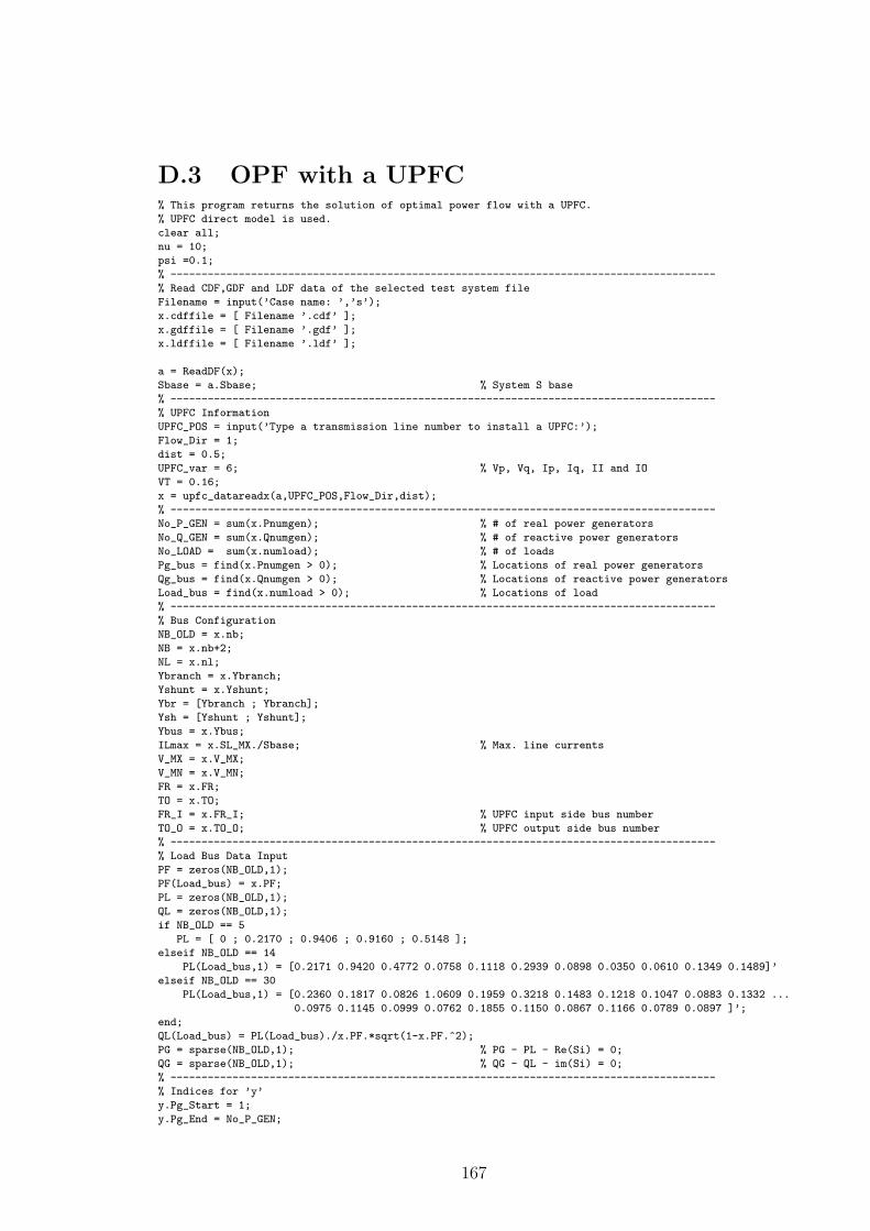
D.3 OPF with a UPFC% This program returns the solution of optimal power flow with a UPFC.
% UPFC direct model is used.
clear all;
nu = 10;
psi =0.1;
% ----------------------------------------------------------------------------------------
% Read CDF,GDF and LDF data of the selected test system file
Filename = input(’Case name: ’,’s’);
x.cdffile = [ Filename ’.cdf’ ];
x.gdffile = [ Filename ’.gdf’ ];
x.ldffile = [ Filename ’.ldf’ ];
a = ReadDF(x);
Sbase = a.Sbase; % System S base
% ----------------------------------------------------------------------------------------
% UPFC Information
UPFC_POS = input(’Type a transmission line number to install a UPFC:’);
Flow_Dir = 1;
dist = 0.5;
UPFC_var = 6; % Vp, Vq, Ip, Iq, II and IO
VT = 0.16;
x = upfc_datareadx(a,UPFC_POS,Flow_Dir,dist);
% ----------------------------------------------------------------------------------------
No_P_GEN = sum(x.Pnumgen); % # of real power generators
No_Q_GEN = sum(x.Qnumgen); % # of reactive power generators
No_LOAD = sum(x.numload); % # of loads
Pg_bus = find(x.Pnumgen > 0); % Locations of real power generators
Qg_bus = find(x.Qnumgen > 0); % Locations of reactive power generators
Load_bus = find(x.numload > 0); % Locations of load
% ----------------------------------------------------------------------------------------
% Bus Configuration
NB_OLD = x.nb;
NB = x.nb+2;
NL = x.nl;
Ybranch = x.Ybranch;
Yshunt = x.Yshunt;
Ybr = [Ybranch ; Ybranch];
Ysh = [Yshunt ; Yshunt];
Ybus = x.Ybus;
ILmax = x.SL_MX./Sbase; % Max. line currents
V_MX = x.V_MX;
V_MN = x.V_MN;
FR = x.FR;
TO = x.TO;
FR_I = x.FR_I; % UPFC input side bus number
TO_O = x.TO_O; % UPFC output side bus number
% ----------------------------------------------------------------------------------------
% Load Bus Data Input
PF = zeros(NB_OLD,1);
PF(Load_bus) = x.PF;
PL = zeros(NB_OLD,1);
QL = zeros(NB_OLD,1);
if NB_OLD == 5
PL = [ 0 ; 0.2170 ; 0.9406 ; 0.9160 ; 0.5148 ];
elseif NB_OLD == 14
PL(Load_bus,1) = [0.2171 0.9420 0.4772 0.0758 0.1118 0.2939 0.0898 0.0350 0.0610 0.1349 0.1489]’
elseif NB_OLD == 30
PL(Load_bus,1) = [0.2360 0.1817 0.0826 1.0609 0.1959 0.3218 0.1483 0.1218 0.1047 0.0883 0.1332 ...
0.0975 0.1145 0.0999 0.0762 0.1855 0.1150 0.0867 0.1166 0.0789 0.0897 ]’;
end;
QL(Load_bus) = PL(Load_bus)./x.PF.*sqrt(1-x.PF.^2);
PG = sparse(NB_OLD,1); % PG - PL - Re(Si) = 0;
QG = sparse(NB_OLD,1); % QG - QL - im(Si) = 0;
% ----------------------------------------------------------------------------------------
% Indices for ’y’
y.Pg_Start = 1;
y.Pg_End = No_P_GEN;
167

y.Qg_Start = y.Pg_End + 1;
y.Qg_End = y.Pg_End + No_Q_GEN;
y.V_Start = y.Qg_End + 1;
y.V_End = y.Qg_End + NB;
y.Theta_Start = y.V_End + UPFC_var + 1;
y.Theta_End = y.V_End + UPFC_var + NB - 1;
y.Pg = y.Pg_Start : y.Pg_End;
y.Qg = y.Qg_Start : y.Qg_End;
y.V = y.V_Start : y.V_End;
y.VI = y.V_End - 1;
y.VO = y.V_End ;
y.Vp = y.V_End + 1;
y.Vq = y.V_End + 2;
y.II = y.V_End + 3;
y.IO = y.V_End + 4;
y.Ip = y.V_End + 5;
y.Iq = y.V_End + 6;
y.Theta = y.Theta_Start : y.Theta_End;
y.thetaI = y.Theta_End-1;
y.thetaO = y.Theta_End;
y.deltaI = y.Theta_End + 1;
y.deltaO = y.Theta_End + 2;
y.Length = y.deltaO;
% ----------------------------------------------------------------------------------------
% Indices for ’lamda’
lamda.P = 1 : NB_OLD;
lamda.Q = NB_OLD+1 : 2*NB_OLD;
lamda.Pin = Pg_bus;
lamda.Qin = Qg_bus + NB_OLD;
lamda.IIinR = 2*NB_OLD + 1;
lamda.IIinI = 2*NB_OLD + 2;
lamda.IOinR = 2*NB_OLD + 3;
lamda.IOinI = 2*NB_OLD + 4;
lamda.IR = 2*NB_OLD + 5;
lamda.II = 2*NB_OLD + 6;
lamda.VR = 2*NB_OLD + 7;
lamda.VI = 2*NB_OLD + 8;
lamda.RP = 2*NB_OLD + 9;
lamda.Length = lamda.RP ;
% ----------------------------------------------------------------------------------------
% Indices for ’mu’
mu.V_MX_Start = 1; % Max. Voltage
mu.V_MX_End = NB;
mu.V_MN_Start = mu.V_MX_End + 1; % Min. Voltage
mu.V_MN_End = mu.V_MX_End + NB;
mu.I_MX_Start = mu.V_MN_End+1; % Max. line current
mu.I_MX_End = mu.V_MN_End + 2*(NL+1);
mu.PgMX_Start = mu.I_MX_End + 1; % Max. real power generation
mu.PgMX_End = mu.I_MX_End + No_P_GEN;
mu.PgMN_Start = mu.PgMX_End+1; % Min. real power generation
mu.PgMN_End = mu.PgMX_End + No_P_GEN;
mu.QgMX_Start = mu.PgMN_End + 1; % Max. reactive power generation
mu.QgMX_End = mu.PgMN_End + No_Q_GEN;
mu.QgMN_Start = mu.QgMX_End+1; % Min. reactive power generation
mu.QgMN_End = mu.QgMX_End + No_Q_GEN;
mu.V_MX = mu.V_MX_Start : mu.V_MX_End ;
mu.V_MN = mu.V_MN_Start : mu.V_MN_End ;
mu.I_MX = mu.I_MX_Start : mu.I_MX_End ;
mu.PgMX = mu.PgMX_Start : mu.PgMX_End ;
mu.PgMN = mu.PgMN_Start : mu.PgMN_End ;
mu.QgMX = mu.QgMX_Start : mu.QgMX_End ;
mu.QgMN = mu.QgMN_Start : mu.QgMN_End ;
mu.VT = mu.QgMN_End + 1;
168

mu.Length = mu.VT ;
% ----------------------------------------------------------------------------------------
% Initial guesses for Pg,Qg,PLoad,V,theta,lamda,mu and s
z = sparse(y.Length,1);
if NB_OLD == 5
z(y.Pg,1) = 1.9847;
z(y.Qg,1) = 0.7155;
z(y.V,1) = [1.0800 ; 1.0651 ; 1.0338 ; 1.0292 ; 1.0361 ; 1.03 ; 1.03 ];
z(y.II,1) = 1.1934;
z(y.IO,1) = 1.1934;
z(y.Theta) = [ -0.0681 ; -0.2008 ; -0.1581 ; -0.1348 ; -0.06 ; -0.06 ];
z(y.deltaI) = 0.05;
z(y.deltaO) = 0.05;
z(y.Vp) = 0.01;
z(y.Vq) = 0.05;
z(y.Ip) = 0.01;
z(y.Iq) = 0.01;
end; % if
if NB_OLD == 14
z=IEEE14_initial(y,UPFC_POS);
end;
if NB_OLD == 30
z(y.Pg,1) = [2.0464 0.4741 0.7209 0.4169 0.1000 0.1000 ]’;
z(y.Qg,1) = [-0.0418 0.0551 0.2553 0.2502 0.1984 0.2660 ]’;
z(y.V,1) = 1.02;
z(y.II,1) = 1.1934;
z(y.IO,1) = 1.1934;
z(y.Theta) = -0.1;
z(y.deltaI) = 0.05;
z(y.deltaO) = 0.05;
z(y.Vp) = 0.01;
z(y.Vq) = 0.05;
z(y.Ip) = 0.01;
z(y.Iq) = 0.01;
end;
LAMDA = 10*ones(lamda.Length,1);
s = ones(mu.Length,1);
S = diag(s);
MU = 10*ones(mu.Length,1);
M = diag(MU);
Z = [z ; LAMDA ; MU; s];
% ----------------------------------------------------------------------------------------
% Indices for "Z"
IX.lamda_Start = y.Length + 1;
IX.lamda_End = y.Length + lamda.Length;
IX.mu_Start = IX.lamda_End + 1;
IX.mu_End = IX.lamda_End + mu.Length;
IX.S_Start = IX.mu_End + 1;
IX.S_End = IX.mu_End + mu.Length;
IX.lamda = IX.lamda_Start : IX.lamda_End;
IX.mu = IX.mu_Start : IX.mu_End;
IX.S = IX.S_Start : IX.S_End;
% ----------------------------------------------------------------------------------------
% Form matrix dh & DDH with constants
dh = sparse(lamda.Length,y.Length); % Jacobian of equality constraints
DDH = sparse(y.Length,y.Length); % Hessian of equality constraints
dh(lamda.Pin,y.Pg) = speye(No_P_GEN,No_P_GEN);
dh(lamda.Qin,y.Qg) = speye(No_Q_GEN,No_Q_GEN);
% ----------------------------------------------------------------------------------------
% Form matrix dg & ddgwith constants
dg = sparse(mu.Length,y.Length); % Jacobian of inequality constraints
DDG = sparse(y.Length,y.Length); % Hessian of inequality constraints
dg(mu.PgMX,y.Pg) = speye(No_P_GEN, No_P_GEN); % For real power generation limit
169

dg(mu.PgMN,y.Pg) = -speye(No_P_GEN, No_P_GEN);
dg(mu.QgMX,y.Qg) = speye(No_Q_GEN, No_Q_GEN); % For reactive power generation limit
dg(mu.QgMN,y.Qg) = -speye(No_Q_GEN, No_Q_GEN);
dg(mu.V_MX,y.V) = speye(NB,NB); % For voltage limit
dg(mu.V_MN,y.V) = -speye(NB,NB);
% ----------------------------------------------------------------------------------------
% Find inequality values
g0 = [-V_MX ; V_MN ; -ILmax.^2 ; -x.Pgmax/Sbase ; x.Pgmin/Sbase ;
-x.Qgmax/Sbase ; x.Qgmin/Sbase ;-VT^2];
% ----------------------------------------------------------------------------------------
% Form matrix ddF
ddF = sparse(y.Length,y.Length);
df0 = sparse(y.Length,1);
ddF(y.Pg,y.Pg) = 2 * diag(x.gamma_c)*Sbase^2;
df0(y.Pg) = x.beta_c*Sbase;
N1 = y.Length; N2 = lamda.Length; N3 = mu.Length; N4 = mu.Length;
i = 0;
while nu > 1e-11 & i < 100
i=i+1;
% ------------------------------------------------------------------------------------
theta = [0 ; Z(y.Theta)];
V = Z(y.V);
Vph = V.*exp(j*theta);
I = Ybus*Vph;
Si = Vph.*conj(I);
PG(Pg_bus) = Z(y.Pg);
QG(Qg_bus) = Z(y.Qg);
% ------------------------------------------------------------------------------------
% Equality constraints "h"
h = zeros(lamda.Length,1);
h(lamda.P,1) = PG-PL-real(Si(1:NB_OLD));
h(lamda.Q,1) = QG-QL-imag(Si(1:NB_OLD));
IIin = Z(y.II)*exp(j*Z(y.deltaI))+Vph(NB-1)*(Ybranch(NL)+Yshunt(NL))-Vph(FR_I)*Ybranch(NL);
IOin =-Z(y.IO)*exp(j*Z(y.deltaO))+Vph(NB)*(Ybranch(NL+1)+Yshunt(NL+1))-Vph(TO_O)*Ybranch(NL+1);
I_Equ= (Z(y.Ip)+j*Z(y.Iq))*exp(j*Z(y.thetaI))+Z(y.IO)*exp(j*Z(y.deltaO))-Z(y.II)*exp(j*Z(y.deltaI));
V_Equ = Vph(NB)-Vph(NB-1)-(Z(y.Vp)+j*Z(y.Vq))*exp(j*Z(y.deltaO));
h(lamda.IIinR) = real(IIin);
h(lamda.IIinI) = imag(IIin);
h(lamda.IOinR) = real(IOin);
h(lamda.IOinI) = imag(IOin);
h(lamda.IR) = real(I_Equ);
h(lamda.II) = imag(I_Equ);
h(lamda.VR) = real(V_Equ);
h(lamda.VI) = imag(V_Equ);
h(lamda.RP) = Z(y.VI)*Z(y.Ip)-Z(y.Vp)*Z(y.IO);
% ------------------------------------------------------------------------------------
% Jacobian of equality constraints "dh"
% Current injection at regular buses
Jsv = diag(Vph)*conj(Ybus)*conj(diag(exp(j*theta)))+diag(exp(j*theta).*conj(I));
Jst = -j*diag(Vph)*conj(Ybus)*conj(diag(Vph))+diag(j*Si);
dh(lamda.P, y.V) = -real(Jsv(1:NB_OLD,:));
dh(lamda.Q, y.V) = -imag(Jsv(1:NB_OLD,:));
dh(lamda.P, y.Theta) = -real(Jst(1:NB_OLD,2:NB));
dh(lamda.Q, y.Theta) = -imag(Jst(1:NB_OLD,2:NB));
% Current injection at UPFC input
dh_IIin = zeros(1,y.Length);
dh_IIin(1,y.V(FR_I)) = -exp(j*theta(FR_I))*Ybranch(NL);
dh_IIin(1,y.VI) = exp(j*Z(y.thetaI))*(Yshunt(NL)+Ybranch(NL));
dh_IIin(1,y.II) = exp(j*Z(y.deltaI));
if FR_I ~= 1 % Bus 1 is the slack bus.
dh_IIin(1,y.Theta(FR_I-1)) = -j*Vph(FR_I)*Ybranch(NL);
end;
dh_IIin(1,y.thetaI) = j*Vph(NB-1)*(Yshunt(NL)+Ybranch(NL));
dh_IIin(1,y.deltaI) = j*Z(y.II)*exp(j*Z(y.deltaI));
% Current injection at UPFC output
170
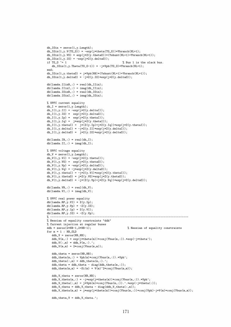
dh_IOin = zeros(1,y.Length);
dh_IOin(1,y.V(TO_O)) = -exp(j*theta(TO_O))*Ybranch(NL+1);
dh_IOin(1,y.VO) = exp(j*Z(y.thetaO))*(Yshunt(NL+1)+Ybranch(NL+1));
dh_IOin(1,y.IO) = -exp(j*Z(y.deltaO));
if TO_O ~= 1 % Bus 1 is the slack bus.
dh_IOin(1,y.Theta(TO_O-1)) = -j*Vph(TO_O)*Ybranch(NL+1);
end;
dh_IOin(1,y.thetaO) = j*Vph(NB)*(Yshunt(NL+1)+Ybranch(NL+1));
dh_IOin(1,y.deltaO) = -j*Z(y.IO)*exp(j*Z(y.deltaO));
dh(lamda.IIinR,:) = real(dh_IIin);
dh(lamda.IIinI,:) = imag(dh_IIin);
dh(lamda.IOinR,:) = real(dh_IOin);
dh(lamda.IOinI,:) = imag(dh_IOin);
% UPFC current equality
dh_I = zeros(1,y.Length);
dh_I(1,y.II) = -exp(j*Z(y.deltaI));
dh_I(1,y.IO) = exp(j*Z(y.deltaO));
dh_I(1,y.Ip) = exp(j*Z(y.thetaI));
dh_I(1,y.Iq) = j*exp(j*Z(y.thetaI));
dh_I(1,y.thetaI) = j*(Z(y.Ip)+j*Z(y.Iq))*exp(j*Z(y.thetaI));
dh_I(1,y.deltaI) = -j*Z(y.II)*exp(j*Z(y.deltaI));
dh_I(1,y.deltaO) = j*Z(y.IO)*exp(j*Z(y.deltaO));
dh(lamda.IR,:) = real(dh_I);
dh(lamda.II,:) = imag(dh_I);
% UPFC voltage equality
dh_V = zeros(1,y.Length);
dh_V(1,y.VI) = -exp(j*Z(y.thetaI));
dh_V(1,y.VO) = exp(j*Z(y.thetaO));
dh_V(1,y.Vp) = -exp(j*Z(y.deltaO));
dh_V(1,y.Vq) = -j*exp(j*Z(y.deltaO));
dh_V(1,y.thetaI) = -j*Z(y.VI)*exp(j*Z(y.thetaI));
dh_V(1,y.thetaO) = j*Z(y.VO)*exp(j*Z(y.thetaO));
dh_V(1,y.deltaO) = -j*(Z(y.Vp)+j*Z(y.Vq))*exp(j*Z(y.deltaO));
dh(lamda.VR,:) = real(dh_V);
dh(lamda.VI,:) = imag(dh_V);
% UPFC real power equality
dh(lamda.RP,y.VI) = Z(y.Ip);
dh(lamda.RP,y.Vp) = -Z(y.IO);
dh(lamda.RP,y.Ip) = Z(y.VI);
dh(lamda.RP,y.IO) = -Z(y.Vp);
% ------------------------------------------------------------------------------------
% Hessian of equality constraints "ddh"
% Current injection at regular buses
ddh = zeros(2*NB-1,2*NB-1); % Hessian of equality constraints
for m = 1 : NB_OLD
ddh_V = zeros(NB,NB);
ddh_V(m,:) = exp(j*theta(m))*conj(Ybus(m,:)).*exp(-j*theta’);
ddh_V(:,m) = ddh_V(m,:).’;
ddh_V(m,m) = 2*conj(Ybus(m,m));
ddh_theta = zeros(NB,NB);
ddh_theta(m,:) = Vph(m)*conj(Ybus(m,:)).*Vph’;
ddh_theta(:,m) = ddh_theta(m,:).’;
ddh_theta = ddh_theta - diag(ddh_theta(m,:));
ddh_theta(m,m) = -Si(m) + V(m)^2*conj(Ybus(m,m));
ddh_V_theta = zeros(NB,NB);
ddh_V_theta(m,:) = -j*exp(j*theta(m))*conj(Ybus(m,:)).*Vph’;
ddh_V_theta(:,m) = j*Vph(m)*conj(Ybus(m,:)).’.*exp(-j*theta(:));
ddh_V_theta = ddh_V_theta - diag(ddh_V_theta(:,m));
ddh_V_theta(m,m) = j*exp(j*theta(m))*conj(Ybus(m,:))*conj(Vph)-j*V(m)*conj(Ybus(m,m));
ddh_theta_V = ddh_V_theta.’;
171
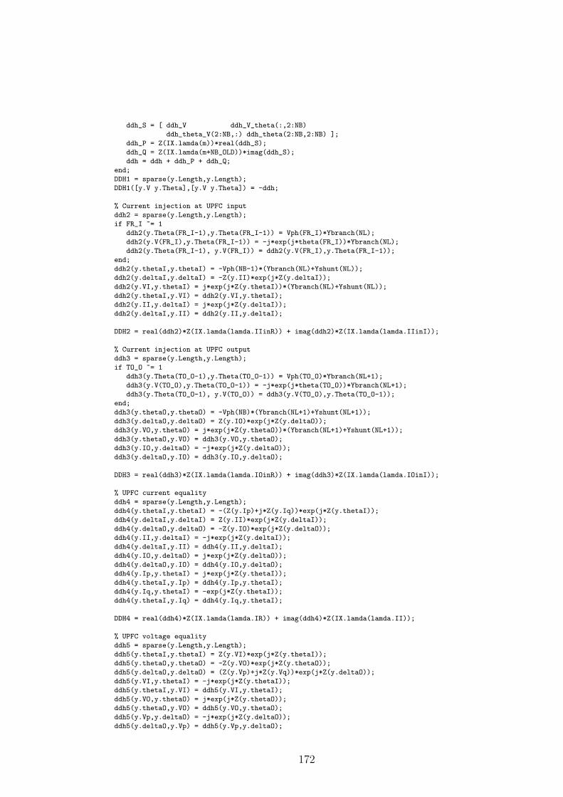
ddh_S = [ ddh_V ddh_V_theta(:,2:NB)
ddh_theta_V(2:NB,:) ddh_theta(2:NB,2:NB) ];
ddh_P = Z(IX.lamda(m))*real(ddh_S);
ddh_Q = Z(IX.lamda(m+NB_OLD))*imag(ddh_S);
ddh = ddh + ddh_P + ddh_Q;
end;
DDH1 = sparse(y.Length,y.Length);
DDH1([y.V y.Theta],[y.V y.Theta]) = -ddh;
% Current injection at UPFC input
ddh2 = sparse(y.Length,y.Length);
if FR_I ~= 1
ddh2(y.Theta(FR_I-1),y.Theta(FR_I-1)) = Vph(FR_I)*Ybranch(NL);
ddh2(y.V(FR_I),y.Theta(FR_I-1)) = -j*exp(j*theta(FR_I))*Ybranch(NL);
ddh2(y.Theta(FR_I-1), y.V(FR_I)) = ddh2(y.V(FR_I),y.Theta(FR_I-1));
end;
ddh2(y.thetaI,y.thetaI) = -Vph(NB-1)*(Ybranch(NL)+Yshunt(NL));
ddh2(y.deltaI,y.deltaI) = -Z(y.II)*exp(j*Z(y.deltaI));
ddh2(y.VI,y.thetaI) = j*exp(j*Z(y.thetaI))*(Ybranch(NL)+Yshunt(NL));
ddh2(y.thetaI,y.VI) = ddh2(y.VI,y.thetaI);
ddh2(y.II,y.deltaI) = j*exp(j*Z(y.deltaI));
ddh2(y.deltaI,y.II) = ddh2(y.II,y.deltaI);
DDH2 = real(ddh2)*Z(IX.lamda(lamda.IIinR)) + imag(ddh2)*Z(IX.lamda(lamda.IIinI));
% Current injection at UPFC output
ddh3 = sparse(y.Length,y.Length);
if TO_O ~= 1
ddh3(y.Theta(TO_O-1),y.Theta(TO_O-1)) = Vph(TO_O)*Ybranch(NL+1);
ddh3(y.V(TO_O),y.Theta(TO_O-1)) = -j*exp(j*theta(TO_O))*Ybranch(NL+1);
ddh3(y.Theta(TO_O-1), y.V(TO_O)) = ddh3(y.V(TO_O),y.Theta(TO_O-1));
end;
ddh3(y.thetaO,y.thetaO) = -Vph(NB)*(Ybranch(NL+1)+Yshunt(NL+1));
ddh3(y.deltaO,y.deltaO) = Z(y.IO)*exp(j*Z(y.deltaO));
ddh3(y.VO,y.thetaO) = j*exp(j*Z(y.thetaO))*(Ybranch(NL+1)+Yshunt(NL+1));
ddh3(y.thetaO,y.VO) = ddh3(y.VO,y.thetaO);
ddh3(y.IO,y.deltaO) = -j*exp(j*Z(y.deltaO));
ddh3(y.deltaO,y.IO) = ddh3(y.IO,y.deltaO);
DDH3 = real(ddh3)*Z(IX.lamda(lamda.IOinR)) + imag(ddh3)*Z(IX.lamda(lamda.IOinI));
% UPFC current equality
ddh4 = sparse(y.Length,y.Length);
ddh4(y.thetaI,y.thetaI) = -(Z(y.Ip)+j*Z(y.Iq))*exp(j*Z(y.thetaI));
ddh4(y.deltaI,y.deltaI) = Z(y.II)*exp(j*Z(y.deltaI));
ddh4(y.deltaO,y.deltaO) = -Z(y.IO)*exp(j*Z(y.deltaO));
ddh4(y.II,y.deltaI) = -j*exp(j*Z(y.deltaI));
ddh4(y.deltaI,y.II) = ddh4(y.II,y.deltaI);
ddh4(y.IO,y.deltaO) = j*exp(j*Z(y.deltaO));
ddh4(y.deltaO,y.IO) = ddh4(y.IO,y.deltaO);
ddh4(y.Ip,y.thetaI) = j*exp(j*Z(y.thetaI));
ddh4(y.thetaI,y.Ip) = ddh4(y.Ip,y.thetaI);
ddh4(y.Iq,y.thetaI) = -exp(j*Z(y.thetaI));
ddh4(y.thetaI,y.Iq) = ddh4(y.Iq,y.thetaI);
DDH4 = real(ddh4)*Z(IX.lamda(lamda.IR)) + imag(ddh4)*Z(IX.lamda(lamda.II));
% UPFC voltage equality
ddh5 = sparse(y.Length,y.Length);
ddh5(y.thetaI,y.thetaI) = Z(y.VI)*exp(j*Z(y.thetaI));
ddh5(y.thetaO,y.thetaO) = -Z(y.VO)*exp(j*Z(y.thetaO));
ddh5(y.deltaO,y.deltaO) = (Z(y.Vp)+j*Z(y.Vq))*exp(j*Z(y.deltaO));
ddh5(y.VI,y.thetaI) = -j*exp(j*Z(y.thetaI));
ddh5(y.thetaI,y.VI) = ddh5(y.VI,y.thetaI);
ddh5(y.VO,y.thetaO) = j*exp(j*Z(y.thetaO));
ddh5(y.thetaO,y.VO) = ddh5(y.VO,y.thetaO);
ddh5(y.Vp,y.deltaO) = -j*exp(j*Z(y.deltaO));
ddh5(y.deltaO,y.Vp) = ddh5(y.Vp,y.deltaO);
172

ddh5(y.Vq,y.deltaO) = exp(j*Z(y.deltaO));
ddh5(y.deltaO,y.Vq) = ddh5(y.Vq,y.deltaO);
DDH5 = real(ddh5)*Z(IX.lamda(lamda.VR)) + imag(ddh5)*Z(IX.lamda(lamda.VI));
% UPFC real power equality
ddh6 = sparse(y.Length,y.Length);
ddh6(y.VI,y.Ip) = 1;
ddh6(y.Ip,y.VI) = 1;
ddh6(y.Vp,y.IO) = -1;
ddh6(y.IO,y.Vp) = -1;
DDH6 = ddh6 * Z(IX.lamda(lamda.RP));
% Construction of total "ddh"
DDH = DDH1 + DDH2 + DDH3 + DDH4 + DDH5 + DDH6;
% ------------------------------------------------------------------------------------
% Inequality constraints "g"
Iik = (Vph(FR)-Vph(TO)).*Ybr+Ysh.*Vph(FR);
gg = zeros(N3,1);
gg(mu.V_MX) = Z(y.V);
gg(mu.V_MN) = -Z(y.V);
gg(mu.I_MX) = Iik.*conj(Iik);
gg(mu.PgMX) = Z(y.Pg);
gg(mu.PgMN) = -Z(y.Pg);
gg(mu.QgMX) = Z(y.Qg);
gg(mu.QgMN) = -Z(y.Qg);
gg(mu.VT) = Z(y.Vp)^2 + Z(y.Vq)^2;
g = gg + g0;
% ------------------------------------------------------------------------------------
% Jacobian of inequality constraints "dg"
% Line flow inequality
dI_dVi = exp(j*theta(FR)).*(Ybr+Ysh);
dI_dVk = -exp(j*theta(TO)).*Ybr;
dIdVi = sparse((1:2*(NL+1)),FR,conj(Iik).*dI_dVi+Iik.*conj(dI_dVi),2*(NL+1),NB);
dIdVk = sparse((1:2*(NL+1)),TO,conj(Iik).*dI_dVk+Iik.*conj(dI_dVk),2*(NL+1),NB);
dIdV = dIdVi + dIdVk;
dg(mu.I_MX,y.V) = dIdV;
dI_dthetai = j*Vph(FR).*(Ybr+Ysh);
dI_dthetak = -j*Vph(TO).*Ybr;
dIidthetai = sparse((1:2*(NL+1)),FR,conj(Iik).*dI_dthetai+Iik.*conj(dI_dthetai),2*(NL+1),NB);
dIidthetak = sparse((1:2*(NL+1)),TO,conj(Iik).*dI_dthetak+Iik.*conj(dI_dthetak),2*(NL+1),NB);
dIdtheta = dIidthetai + dIidthetak;
dg(mu.I_MX,y.Theta) = dIdtheta(:,2:NB);
% Injected voltage magnitude inequality
dg(mu.VT,y.Vp) = 2 * Z(y.Vp);
dg(mu.VT,y.Vq) = 2 * Z(y.Vq);
% ------------------------------------------------------------------------------------
% Hessian of inequality constraints "ddg"
ddg = zeros(2*NB-1,2*NB-1);
for m = 1 : 2*(NL+1)
ddg_V = sparse(NB,NB);
ddg_V(FR(m),FR(m)) = 2*conj(dI_dVi(m))*dI_dVi(m);
ddg_V(FR(m),TO(m))= conj(dI_dVk(m))*dI_dVi(m) + dI_dVk(m)*conj(dI_dVi(m));
ddg_V(TO(m),FR(m)) = ddg_V(FR(m),TO(m));
ddg_V(TO(m),TO(m)) = 2*conj(dI_dVk(m))*dI_dVk(m);
ddg_theta = sparse(NB,NB);
ddI_ddthetaii = -(Ybr(m)+Ysh(m))*Vph(FR(m));
ddg_theta(FR(m),FR(m)) = Iik(m)’* ddI_ddthetaii+2*conj(dI_dthetai(m))*...
dI_dthetai(m) + Iik(m)*conj(ddI_ddthetaii);
ddg_theta(FR(m),TO(m))= dI_dthetai(m)’*dI_dthetak(m)+dI_dthetai(m)*dI_dthetak(m)’;
ddg_theta(TO(m),FR(m))= ddg_theta(FR(m),TO(m));
ddI_ddthetakk = Ybr(m)*Vph(TO(m));
173
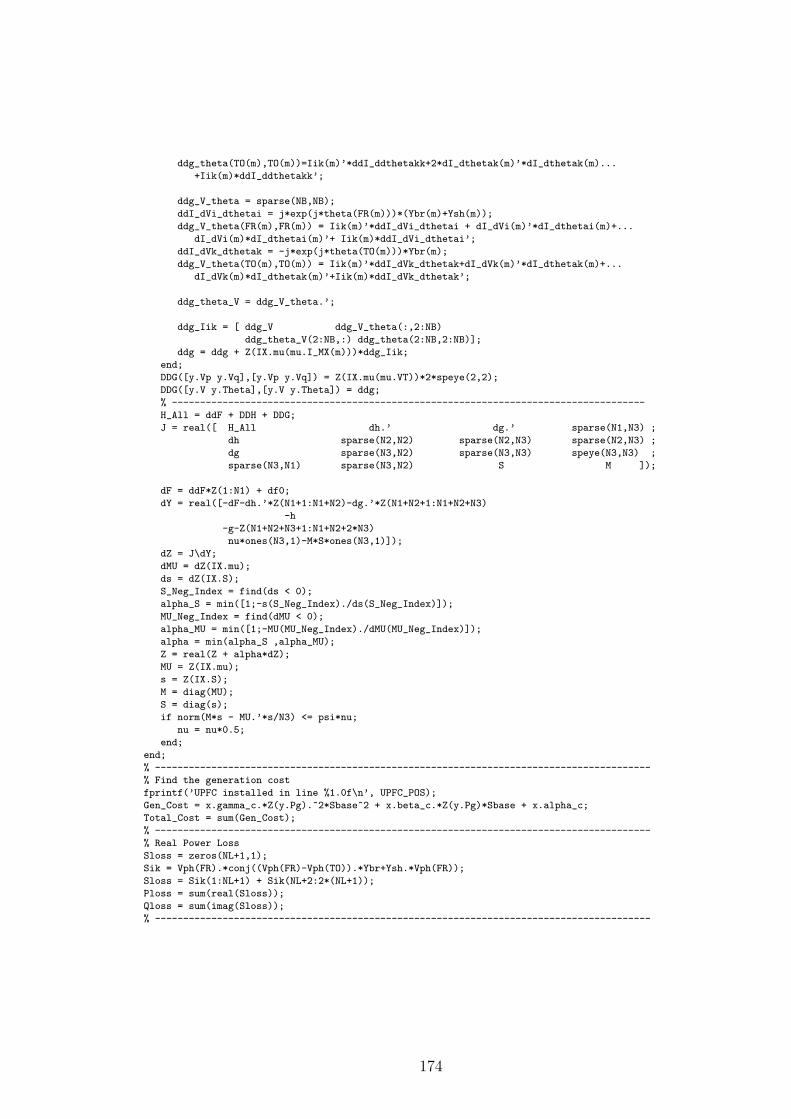
ddg_theta(TO(m),TO(m))=Iik(m)’*ddI_ddthetakk+2*dI_dthetak(m)’*dI_dthetak(m)...
+Iik(m)*ddI_ddthetakk’;
ddg_V_theta = sparse(NB,NB);
ddI_dVi_dthetai = j*exp(j*theta(FR(m)))*(Ybr(m)+Ysh(m));
ddg_V_theta(FR(m),FR(m)) = Iik(m)’*ddI_dVi_dthetai + dI_dVi(m)’*dI_dthetai(m)+...
dI_dVi(m)*dI_dthetai(m)’+ Iik(m)*ddI_dVi_dthetai’;
ddI_dVk_dthetak = -j*exp(j*theta(TO(m)))*Ybr(m);
ddg_V_theta(TO(m),TO(m)) = Iik(m)’*ddI_dVk_dthetak+dI_dVk(m)’*dI_dthetak(m)+...
dI_dVk(m)*dI_dthetak(m)’+Iik(m)*ddI_dVk_dthetak’;
ddg_theta_V = ddg_V_theta.’;
ddg_Iik = [ ddg_V ddg_V_theta(:,2:NB)
ddg_theta_V(2:NB,:) ddg_theta(2:NB,2:NB)];
ddg = ddg + Z(IX.mu(mu.I_MX(m)))*ddg_Iik;
end;
DDG([y.Vp y.Vq],[y.Vp y.Vq]) = Z(IX.mu(mu.VT))*2*speye(2,2);
DDG([y.V y.Theta],[y.V y.Theta]) = ddg;
% ------------------------------------------------------------------------------------
H_All = ddF + DDH + DDG;
J = real([ H_All dh.’ dg.’ sparse(N1,N3) ;
dh sparse(N2,N2) sparse(N2,N3) sparse(N2,N3) ;
dg sparse(N3,N2) sparse(N3,N3) speye(N3,N3) ;
sparse(N3,N1) sparse(N3,N2) S M ]);
dF = ddF*Z(1:N1) + df0;
dY = real([-dF-dh.’*Z(N1+1:N1+N2)-dg.’*Z(N1+N2+1:N1+N2+N3)
-h
-g-Z(N1+N2+N3+1:N1+N2+2*N3)
nu*ones(N3,1)-M*S*ones(N3,1)]);
dZ = J\dY;
dMU = dZ(IX.mu);
ds = dZ(IX.S);
S_Neg_Index = find(ds < 0);
alpha_S = min([1;-s(S_Neg_Index)./ds(S_Neg_Index)]);
MU_Neg_Index = find(dMU < 0);
alpha_MU = min([1;-MU(MU_Neg_Index)./dMU(MU_Neg_Index)]);
alpha = min(alpha_S ,alpha_MU);
Z = real(Z + alpha*dZ);
MU = Z(IX.mu);
s = Z(IX.S);
M = diag(MU);
S = diag(s);
if norm(M*s - MU.’*s/N3) <= psi*nu;
nu = nu*0.5;
end;
end;
% ----------------------------------------------------------------------------------------
% Find the generation cost
fprintf(’UPFC installed in line %1.0f\n’, UPFC_POS);
Gen_Cost = x.gamma_c.*Z(y.Pg).^2*Sbase^2 + x.beta_c.*Z(y.Pg)*Sbase + x.alpha_c;
Total_Cost = sum(Gen_Cost);
% ----------------------------------------------------------------------------------------
% Real Power Loss
Sloss = zeros(NL+1,1);
Sik = Vph(FR).*conj((Vph(FR)-Vph(TO)).*Ybr+Ysh.*Vph(FR));
Sloss = Sik(1:NL+1) + Sik(NL+2:2*(NL+1));
Ploss = sum(real(Sloss));
Qloss = sum(imag(Sloss));
% ----------------------------------------------------------------------------------------
174