natural selection along an environmental gradient: …

ORIGINAL ARTICLE

doi:10.1111/j.1558-5646.2008.00425.x

NATURAL SELECTION ALONG ANENVIRONMENTAL GRADIENT: A CLASSICCLINE IN MOUSE PIGMENTATIONLynne M. Mullen1,2 and Hopi E. Hoekstra1,3

1Department of Organismic and Evolutionary Biology and The Museum of Comparative Zoology,

Harvard University, 26 Oxford Street, Cambridge, Massachusetts 021382E-mail: [email protected]: [email protected]

Received January 30, 2008

Accepted April 22, 2008

We revisited a classic study of morphological variation in the oldfield mouse (Peromyscus polionotus) to estimate the strength of

selection acting on pigmentation patterns and to identify the underlying genes. We measured 215 specimens collected by Francis

Sumner in the 1920s from eight populations across a 155-km, environmentally variable transect from the white sands of Florida’s

Gulf coast to the dark, loamy soil of southeastern Alabama. Like Sumner, we found significant variation among populations:

mice inhabiting coastal sand dunes had larger feet, longer tails, and lighter pigmentation than inland populations. Most striking,

all seven pigmentation traits examined showed a sharp decrease in reflectance about 55 km from the coast, with most of the

phenotypic change occurring over less than 10 km. The largest change in soil reflectance occurred just south of this break in

pigmentation. Geographic analysis of microsatellite markers shows little interpopulation differentiation, so the abrupt change in

pigmentation is not associated with recent secondary contact or reduced gene flow between adjacent populations. Using these

genetic data, we estimated that the strength of selection needed to maintain the observed distribution of pigment traits ranged

from 0.0004 to 21%, depending on the trait and model used. We also examined changes in allele frequency of SNPs in two

pigmentation genes, Mc1r and Agouti, and show that mutations in the cis-regulatory region of Agouti may contribute to this cline

in pigmentation. The concordance between environmental variation and pigmentation in the face of high levels of interpopulation

gene flow strongly implies that natural selection is maintaining a steep cline in pigmentation and the genes underlying it.

KEY WORDS: Adaptation, Agouti, color, Haldane, Mc1r, natural selection, Peromyscus.

Clinal variation can provide strong evidence for adaptation to

different environments. Although there are many examples of

clines in allele frequencies (e.g., Berry and Kreitman 1993; Eanes

1999; Schmidt and Rand 2001; Fry et al. 2008), often a precise

understanding of the selective agent responsible for producing

the cline is lacking. On the other hand, there are many examples

of clines in phenotypic traits (reviewed in Endler 1977; Hedrick

2006; Schemske and Bierzychudek 2007), but in most cases we

do not know their genetic basis. Thus, there are few cases in which

clinal variation in both phenotype and its underlying genes have

been examined in an ecological context (but see Caicedo et al.

2004; Hoekstra et al. 2004). Here, we revisit a classic evolutionary

study of deer mice (genus Peromyscus) conducted by Francis

Bertody Sumner nearly a century ago to determine the role of

natural selection in maintaining clinal variation in pigmentation

and to identify the underlying genetics.

In the summer of 1924, after more than 20 years of studying

geographic variation in Peromyscus in the western United States,

Francis Sumner traveled to Florida, “where material has been

found which promises to yield more valuable returns than any

which have thus far been reported” (Sumner 1926, p. 149). Sumner

was referring to the widespread species Peromyscus polionotus,

1 5 5 5C© 2008 The Author(s). Journal compilation C© 2008 The Society for the Study of Evolution.Evolution 62-7: 1555–1570

L. M. MULLEN AND H. E. HOEKSTRA

which, throughout most of its range in the southeastern US, has

a dark brown dorsal coat, striped tail, and light gray ventrum.

A colleague, however, had recently reported the existence of a

unique race, P. p. leucocephalus, on a barrier island off the Gulf

Coast of Florida (Howell 1920)—a race with “paler coloration

and more extensive white areas than any other wild mouse with

which [Sumner was] acquainted” (Sumner 1929a, p. 110).

During 1926 and 1927, Sumner collected, measured, and

prepared museum skins for over 400 mice from eight localities

spanning over 150 km from a coastal population in Florida north-

ward into Alabama. As Sumner found, P. polionotus occupied an

environmental gradient ranging from the vegetatively depauper-

ate, brilliant white sandy beaches of Florida’s Gulf coast to inland

areas, particularly densely vegetated oldfields.

Sumner’s two-year effort produced not only laboratory stocks

derived from the two extreme forms (taken from end points of

his transect), but also an extensive series of museum skins. In the

laboratory, crosses among light and dark forms convinced Sumner

that (1) the difference in coat color between the beach and inland

form was genetic and controlled by a handful of loci, and (2)

the two extreme forms were interfertile and thus could exchange

genetic material in the wild (Sumner 1930). Sumner also used his

study skins to examine variation in nature. He found that, about

50 km from the coast, the pale-colored mouse was replaced rather

abruptly by a darker form more typical of the genus—a narrow

“area of intergradation,” (Sumner 1929a,b). Taken together, these

observations were puzzling: why was there such an abrupt change

in pigmentation if the mice were interfertile?

Several answers have been offered. Sumner speculated that

these distinct racial differences were largely caused by the range

expansion of light mice into the previously allopatric range of dark

mice (Sumner 1929b). Bowen (1968) also believed that the two

divergent forms had recently come into contact, but he empha-

sized that ecological barriers were necessary to limit intermixing

between them and that selection need not be invoked to explain

the observed cline. Still others favored the idea that strong disrup-

tive selection was imposed by a sharp break in soil color, so that

mismatched hybrid offspring had low survival (Haldane 1948).

This last explanation gained favor, and Sumner’s work on this

transect became a classic textbook example of adaptation, widely

discussed in the evolutionary literature (Dobzhansky 1937; Mayr

1942, 1954, 1963; Huxley 1943; Haldane 1948; Ford 1954, 1960,

1964). The pervasive interest in this example comes from its in-

stantiation of selection in action.

In his now-famous 1948 paper, “The theory of a cline,” J.

B. S. Haldane used Sumner’s transect as an example of how

to estimate selection coefficients from geographic variation in

allele frequencies. (Haldane analyzed one trait, the cheek patch,

whose variation, he assumed, was caused by allelic differences at

a single locus). Haldane concluded that selection on cheek patch

color was strong, but added that this conclusion relied on several

untested assumptions about, for example, migration rates and the

underlying genetics.

By returning to this classic system armed with modern molec-

ular tools and more sophisticated mathematical methods, we can

gain new insight into how the interaction between selection, de-

mography, and genetics generates this striking cline in pigmen-

tation. Here, we tested the three alternative hypotheses about the

genetic structure of Sumner’s mouse populations and showed that

habitat-specific natural selection is responsible for clinal variation

in pigmentation. We also estimated the strength of selection acting

on pigmentation by supplying the missing genetic data called for

by Haldane. Finally, we determined geographic changes in allele

frequencies of candidate pigmentation genes in an effort to iden-

tify genes and mutations responsible for this cline in coat color.

All these data were gathered using Sumner’s original museum

collections of P. polionotus.

Methods and MaterialsMOUSE SAMPLES

We sampled 215 museum specimens caught by Sumner in 1927

and now accessioned at the University of California-Berkeley

Museum of Vertebrate Zoology. These mice were collected along

a southwest-to-northeast transect spanning 155 km from St.

Andrews Bay, Florida to southeastern Alabama (Fig. 1; Sumner

1929). Table 1 provides detailed locality data. We characterized

morphological and genetic diversity in 22–25 samples from each

of eight sampling locales with one exception: we sampled 43 indi-

viduals from one “population” [Intergrades (IN)]. The Intergrades

site comprises four localities no more than 4 km apart, and these

localities span the heterogeneity in soil color at the center of the

transect. Accession numbers for each mouse are listed by collect-

ing site in online Supplementary Table S1.

Geographic distances between collection sites were calcu-

lated with the GEOD (http://www.indo.com/distance/) program

from the U.S. Geological Survey. Because the sampling transect

is not perfectly linear, we used measures of latitude as a proxy

for actual distance between the populations. The average distance

between collecting sites was 15.5 km (± 22.0 km), which is larger

than the estimated dispersal distance for these mice (Blair 1951;

Swilling and Wooten 2002), and therefore each population can be

considered independent.

LINEAR MEASUREMENTS

To quantify morphological variation, we recorded four standard

museum measurements (to the nearest 0.5 mm) for each specimen:

hindfoot length (distance from heel to middle digit), tail length

(base to tip), ear length (ear base to the most distant tip), and body

length (from tip of the rostrum to the base of the tail). Online Sup-

plementary Table S2 gives trait means for mice from each of the

1 5 5 6 EVOLUTION JULY 2008

CLINAL SELECTION IN PEROM YSCUS

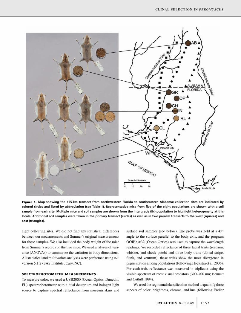
Figure 1. Map showing the 155-km transect from northwestern Florida to southeastern Alabama; collection sites are indicated by

colored circles and listed by abbreviation (see Table 1). Representative mice from five of the eight populations are shown with a soil

sample from each site. Multiple mice and soil samples are shown from the Intergrade (IN) population to highlight heterogeneity at this

locale. Additional soil samples were taken in the primary transect (circles) as well as in two parallel transects to the west (squares) and

east (triangles).

eight collecting sites. We did not find any statistical differences

between our measurements and Sumner’s original measurements

for these samples. We also included the body weight of the mice

from Sumner’s records on the live mice. We used analyses of vari-

ance (ANOVAs) to summarize the variation in body dimensions.

All statistical and multivariate analyses were performed using JMP

version 5.1.2 (SAS Institute, Cary, NC).

SPECTROPHOTOMETER MEASUREMENTS

To measure color, we used a USB2000 (Ocean Optics, Dunedin,

FL) spectrophotometer with a dual deuterium and halogen light

source to capture spectral reflectance from museum skins and

surface soil samples (see below). The probe was held at a 45◦

angle to the surface parallel to the body axis, and the program

OOIBASE32 (Ocean Optics) was used to capture the wavelength

readings. We recorded reflectance of three facial traits (rostrum,

whisker, and cheek patch) and three body traits (dorsal stripe,

flank, and ventrum); these traits show the most divergence in

pigmentation among populations (following Hoekstra et al. 2006).

For each trait, reflectance was measured in triplicate using the

visible spectrum of most visual predators (300–700 nm; Bennett

and Cuthill 1994).

We used the segmental classification method to quantify three

aspects of color: brightness, chroma, and hue (following Endler

EVOLUTION JULY 2008 1 5 5 7


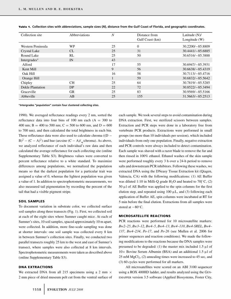
Table 1. Collection sites with abbreviations, sample sizes (N), distance from the Gulf Coast of Florida, and geographic coordinates.

Collection site Abbreviations N Distance from Latitude (N)/Gulf Coast (km) Longitude (W)

Western Peninsula WP 25 0 30.2200/−85.8809Crystal Lake CL 25 31 30.4441/−85.6885Round Lake RL 25 50 30.6516/−85.3888Intergrades∗ IN 43Alford 17 55 30.6947/−85.3931Kent Mill 9 56 30.6638/−85.4319Oak Hill 16 58 30.7113/−85.4716Orange Hill 1 59 30.6832/−85.5642

Chipley CH 25 64 30.7819/−85.5285Dekle Plantation DP 22 72 30.8522/−85.3494Graceville GR 25 83 30.9569/−85.5166Abbeville AB 25 155 31.5663/−85.2513

∗Intergrades “population” contain four clustered collecting sites.

1990). We averaged reflectance readings every 2 nm, sorted the

reflectance data into four bins of 100 nm each (A = 300 to

400 nm; B = 400 to 500 nm; C = 500 to 600 nm, and D = 600

to 700 nm), and then calculated the total brightness in each bin.

These reflectance data were also used to calculate chroma ((D −B)2 − (C − A)2) and hue (arcsine (C − A)/√chroma). As above,

we analyzed reflectance of each individual’s raw data and then

calculated the average reflectance for each collecting site (online

Supplementary Table S3). Brightness values were converted to

percent reflectance relative to a white standard. To maximize

differences among populations, we normalized the population

means so that the darkest population for a particular trait was

assigned a value of 0, whereas the lightest population was given

a value of 1. In addition to spectrophotometric measurements, we

also measured tail pigmentation by recording the percent of the

tail that had a visible pigment stripe.

SOIL SAMPLES

To document variation in substrate color, we collected surface

soil samples along three transects (Fig. 1). First, we collected soil

at each of the eight sites where Sumner caught mice. At each of

Sumner’s sites, 10 soil samples, spaced approximately 10 m apart,

were collected. In addition, more fine-scale sampling was done

at shorter intervals: one soil sample was collected every 8 km

in between Sumner’s collection sites. Finally, we conducted two

parallel transects roughly 25 km to the west and east of Sumner’s

transect, where samples were also collected at 8 km intervals.

Spectrophotometric measurements were taken as described above

(online Supplementary Table S3).

DNA EXTRACTIONS

We extracted DNA from all 215 specimens using a 2 mm ×2 mm piece of dried museum pelt cut from the ventral surface of

each sample. We took several steps to avoid contamination during

DNA extraction. First, we sterilized scissors between samples.

Extraction and PCR steps were done in a laboratory free from

vertebrate PCR products. Extractions were performed in small

groups (no more than 10 individuals per session), which included

individuals from only one population. Finally, negative extraction

and PCR controls were always included to detect contamination.

Each sample was shaved with a razor blade to remove the fur and

then rinsed in 100% ethanol. Ethanol washes of the skin sample

were performed roughly every 3 h over a 24-h period to remove

salts and downstream PCR inhibitors. Following these washes, we

extracted DNA using the DNeasy Tissue Extraction kit (Qiagen,

Valencia, CA) with the following modifications: (1) AE Buffer

was diluted 1:10 in Milli-Q grade H2O and heated to 70[◦C, (2)

50 μl of AE Buffer was applied to the spin columns for the first

elution step, and repeated using 100 μL, and (3) following each

application of Buffer AE, spin columns were incubated at RT for

5 min before the final elution. Extractions from all samples were

stored at −80◦C.

MICROSATELLITE REACTIONS

PCR reactions were performed for 10 microsatellite markers:

Bw2–25, Bw3–12, Bw4–5, Bw4–13, Bw4–110, Bw4-SREL, Bw4–

137, Bw4–234, Po-17, and Po-26 (see Mullen et al. 2006 for

primer sequences and reaction conditions). We made the follow-

ing modifications to the reactions because the DNA samples were

presumed to be degraded: (1) the master mix included 1.5 μl of

10× Bovine Serum Albumin (BSA) and an additional 1.5 μl of

25 mM MgCl2, (2) annealing times were increased to 45 sec, and

(3) 60 cycles were performed for all markers.

All microsatellites were scored on an ABI 3100 sequencer

using a ROX 400HD ladder, and results analyzed using the GEN-

EMAPPER version 3.5 software (Applied Biosystems, Foster City,



CA). Because null alleles and allelic dropout are often seen in

studies that use highly degraded DNA specimens (Taberlet et al.

1996; Bonin et al. 2004), we used several strategies to closely

monitor results from microsatellite markers. First, we ran three

replicates of all markers for a subset of 20 individuals to judge the

error rate for each marker, which we found to be low (< 5%). The

amount of DNA present in all samples was also measured with a

SYBR green quantitative PCR reaction, using marker Bw4–137.

The minimum threshold for a sample’s use was set at 25 pg, as

lower values tend to yield high rates of allelic dropout (Morin

et al. 2001). We calculated observed and expected heterozygos-

ity as well as the number of alleles using the program GENALEX

version 6 (Peakall and Smouse 2006). Deviations from Hardy–

Weinberg equilibrium were calculated using exact tests imple-

mented in GENEPOP version 3.4 (Raymond and Rousset 1995) to

identify markers with a deficiency in heterozygote genotypes.

ANALYSIS OF POPULATION STRUCTURE

Data from all 10 microsatellite markers were used to estimate

levels of gene flow and genetic differentiation between adjacent

populations and among all populations. To determine the degree

of genetic structure, we calculated FST using the program AR-

LEQUIN version 2.000 (Schneider et al. 2000). We also calculated

RST values, which are based on a stepwise mutation model most

appropriate for microsatellites (Slatkin 1995). Because RST values

did not differ statistically from FST, we report only FST values

here. To test for a pattern of isolation by distance, we regressed

linearized FST [FST /(1 − FST)] against distance (km) between

sampling locales. Maximum-likelihood (ML) estimates of the per-

generation effective number of migrants (Nm) between pairwise

populations were calculated with the program MIGRATE version

2.0.3 (Beerli and Felsenstein 1999). We initially used MIGRATE de-

fault parameters, and then optimized the likelihood score by using

values from the previous run as the next run’s starting parameters

until the ln (L) peaked and stabilized.

To further characterize the extent of genetic structure among

populations, we used the Bayesian clustering program STRUC-

TURE version 2.0 (Pritchard et al. 2000) to probabilistically assign

individuals to subpopulations (k) independently of sampling ar-

eas. We first tested the hypothesis that two previously isolated

(and genetically distinct) populations have recently come into

contact by constraining our analyses to k = 2. We then sepa-

rately calculated the maximum-likelihood estimate of the number

of subpopulations using the admixture-with-uncorrelated-allele-

frequencies model with a burn-in of 30,000 Markov Chain Monte

Carlo (MCMC) steps followed by 100,000 iterations. The highest

value of k from the average of 10 runs for k = 1 – 11 (where

the highest exploratory k was determined by using the number

of populations sampled plus three) was confirmed with the � k

algorithm (Evanno et al. 2005).

To determine whether variation in pigmentation is best ex-

plained by geographic or genetic distance, we examined statistical

associations among three matrices: (1) variation in pigmentation

among populations, (2) genetic differentiation, and (3) geographic

distance, by performing Matrix Correspondence Tests (MCTs)

using LAPROGICIEL version R 4.0 (Casgrain and Legendre 2001).

MCTs use a regression design to test for multiple correlations be-

tween matrices and use permutation methods to assess statistical

significance. We performed pairwise MCTs to test for correla-

tion between relative brightness values averaged over all traits

(pigmentation), geographical distance (geography), and genetic

distance (linearized FST). Partial MCTs were used to detect cor-

relations between two variables (pigmentation and geography, or

pigmentation and genetic distance) while controlling for the effect

of the third (either genetic distance or geography, respectively).

ANALYSIS OF CLINE SHAPE

To mathematically describe clinal variation, we generated

maximum-likelihood curves for each pigmentation phenotype us-

ing the one-dimensional transect option in the program ANALYSE

version 1.30 (Barton and Baird 1995), which fits sigmoidal tanh

curves to cline data and searches for the maximum-likelihood es-

timates of cline parameters using a Metropolis Hastings algorithm

(Szymura and Barton 1986). We allowed four parameters to vary

for each trait: pmin, pmax (minimum and maximum frequencies at

the tails of the cline, respectively), cline center, and cline width.

Cline center is the distance between the geographic position where

the maximum slope occurs and the first (beach) population. For

phenotypic traits, cline width is calculated using the equation w =�z/(∂z/∂t), where �z is the difference in population means on

each side of the cline and ∂z/∂t is the maximum slope (Barton and

Gale 1993). For allele frequencies, cline width is calculated using

the inverse of the maximum slope. Because extensive sampling

was not performed at the ends of the cline, we did not explore

the stepped-cline model. Body measurements were not analyzed

using this approach, as they did not vary clinally.

To test for statistical concordance among clines (for both

phenotypic traits and allele frequencies), we used likelihood-ratio

tests to compare cline centers and widths (per Phillips et al. 2004).

We constructed likelihood profiles by summing the highest log-

likelihood scores generated by ANALYSE for all phenotypes to

yield an ML estimate of a cline parameter shared by all traits. We

subtracted these profiles from the sum of the ML scores for each

trait and used likelihood ratio tests to determine if cline centers

(or widths) were statistically different. The likelihood test follows

a χ2 distribution, in which the degrees of freedom are equal to the

difference in the number of parameters between each model (in

this case, the number of phenotype — 1). For both cline center

and width estimates, we calculated the ± 2 log L range, which is

equivalent to 95% confidence intervals (Edwards 1992).



ESTIMATING SELECTION COEFFICIENTS

We used two methods to estimate the strength of selection act-

ing on pigmentation. We first used a model that assumes the

environment changes gradually across the transect, in which dis-

persal distance is much smaller than the cline width (the gradient

model). This model assumes the equation b = l2 (2.40/w)3, in

which w is the width of the cline, l is the standard deviation of

the adult-offspring dispersal distance, and b represents the selec-

tion gradient (Endler 1977). We also used a model that assumes a

step-like change in the environment, in which dispersal distance

is similar to or larger than the cline width (the ecotone model).

This model uses the equation w = σ/√s, in which w is the width

of the cline, σ is the standard deviation of the adult-offspring dis-

persal distance, and s is the selection coefficient (Haldane 1948;

Bazykin 1969; Slatkin 1973). We did not directly estimate disper-

sal distance in these populations, and instead used an estimate of

subadult dispersal (0.260 km) taken from mark–recapture studies

of P. polionotus (Blair 1946; Swilling and Wooten 2002).

ALLELIC VARIATION IN CANDIDATE

PIGMENTATION GENES

To identify genetic regions that may underlie clinal variation in

pigmentation, we focused on two candidate genes. Previous work

using a genetic mapping approach identified the melanocortin-

1 receptor (Mc1r) and the Agouti signaling protein (Agouti), as

major contributors to the phenotypic differences between two re-

lated subspecies, the light-colored Santa Rosa Island beach mouse

(P. p. leucocephalus) and a darker mainland subspecies (P. p. sub-

griseus; Steiner et al. 2007). Although these subspecies are dif-

ferent from those studied here (and occur in different areas), they

show a similar divergence of phenotypes.

To determine if allelic variation at Mc1r and Agouti con-

tributes to clinal variation in pigmentation, we measured allele

frequencies within and between populations. For Mc1r, we geno-

typed a single nucleotide mutation in the coding region, which

codes for an amino acid change known to decrease the recep-

tor activity in laboratory experiments (Hoekstra et al. 2006). For

Agouti, expression differences (as opposed to amino acid change)

are correlated with variation in pigmentation, but the causal mu-

tation(s) have not yet been identified (Steiner et al. 2007). There-

fore, we genotyped four single nucleotide polymorphisms (SNPs)

that span 100 kb of the Agouti regulatory region (approximately

2 kb, 40 kb, 50 kb and 100 kb 5′ of exon 2), as these may be

in linkage disequilibrium (LD) with a causal mutation. We used

alignments of several vertebrate Agouti sequences in GenBank

to design conserved primers and amplify about 1 kb regions in

Peromyscus. In these regions, we identified SNPs that were fixed

differences between three mainland (P. p. subgriseus) and three

beach mice (P. p. leucocephalus) from which we had fresh, non-

degraded DNA samples. For all SNPs, we define the “dark” allele

as the allele present in the mainland population and the “light”

allele as the allele present in the beach population.

For four of the five SNPs, we designed custom TaqMan SNP

assays (Applied Biosystems). Online Supplementary Table S4

provides the primer and probe sequences. We conducted all reac-

tions in 13 μl reaction volumes containing 3 μL DNA, 6.25 μl 2X

TaqMan Universal PCR Master Mix (Applied Biosystems), 1.5 μl

10X BSA, and 0.3125 μl custom probe. We genotyped SNPs on an

ABI Prism 7000 using an initial AmpErase uracil-N-glycosylase

(UNG) activation step of 50◦C for 2 min, a denaturation step of

95◦C for 10 min followed by 40 cycles of 94◦C for 15 sec and

60◦C for 1 min. We scored SNPs with the Allelic Discrimination

Assay procedure in SDS version 1.1 (Applied Biosystems).

For one Agouti SNP, located 100 kb upstream of exon 2,

we could not design a TaqMan probe. Therefore, we PCR-

amplified and sequenced 235 bps using primers Ag5 F (5′

AACTTGCTTTGTAGACC 3′) and Ag5 R (5′ TGGGGGAATC-

CAACCTG 3′). We performed PCR reactions in a 15 μl volume

with 2 μl of template DNA, 10× Taq Buffer (1.5mM MgCl2;

Eppendorf), 1.5 μl of 25 mM MgCl2, 1.5 μl 10× BSA, 0.3 μl

of 10 μM dNTPs, 0.6 μL of each 10 μM primer, and 0.2 U of

Taq DNA Polymerase (Eppendorf, Westbury, NY). Reaction con-

ditions were as follows: an initial denaturation step of 94◦C for

3 min, followed by 60 cycles of denaturation at 94◦C for 30 sec,

annealing at 58.8◦C for 45 sec and extension at 72◦C for 1 min.

We performed a final extension step at 72 ◦C for 10 min.

We purified PCR products by adding 0.08 μl Exonuclease

I and 0.4 μl Shrimp Alkaline Phosphatase (USB Corporation,

Cleveland, OH) in a total volume of 5 μl to each sample. Samples

were incubated at 37◦C for 15 min then heated to 80◦C for 15 min.

We sequenced the products with BigDye version 3.1 (Applied

Biosystems) using PCR primers and ran them on an ABI 3100

Genetic Analyzer. We visualized and aligned sequences by eye

using SEQUENCHER version 4.1 (Gene Codes Corporation, Ann

Arbor, MI).

ANALYSIS OF LINKAGE DISEQUILIBRIUM

BETWEEN SNPs

Because the phenotypic effects of Mc1r are dependent on the

Agouti genetic background (Steiner et al. 2007), we used the

program TASSEL version 2.1 (Bradbury et al. 2007) to estimate

linkage disequilibrium (LD) between all pairwise combinations

of Mc1r and Agouti SNPs. We used two ways to test for non-

random associations between SNPs. First, r2 values estimate the

correlation between two loci. Since r2 values depend on allele

frequencies (Hedrick 1987), we also calculated the normalized

disequilibrium coefficient, D′, which is directly related to the

extent of recombination between two loci. Both r2 and D′ val-

ues range from 0 to 1, where 0 represents linkage equilibrium

and 1 indicates complete linkage disequilibrium. We ran 10,000



permutations and used a two-sided Fisher’s exact test to calculate

significance.

ASSOCIATION BETWEEN GENOTYPE

AND PHENOTYPE

For each of the five SNPs, we assigned individuals to one of three

genotypic classes, comprising homozygotes for the light allele,

homozygotes for the dark allele, or heterozygotes. We first tested

for a statistical association between genotype and each of the

seven pigmentation traits using Kruskal–Wallis nonparametric

tests. Because of the potential interaction between loci, we also

tested for an association between genotypic class, when genotypes

at both Mc1r and Agouti were considered simultaneously (a total

of nine genotypic classes), and each pigmentation trait.

ResultsMORPHOLOGICAL VARIATION

To determine the relationship between morphology and geo-

graphic distance, we plotted average values for both body dimen-

sion and pigmentation traits for each of eight populations against

distances and conducted multivariate ANOVAs (Fig. 2). Because

males and females did not differ statistically for any traits, we

combined the sexes in our analysis.

For two body traits we found significant variation among

populations, foot length (F1,203 = 4.31, P = 0.031) and tail length

(F1,212 = 3.79, P = 0.030), as well as a correlation between these

traits and distance (Fig. 2A). This pattern is driven entirely by

the extreme phenotypes in the beach population—most of the

change in foot length (> 1.5 mm) and tail length (> 5.5 mm) oc-

curs between the coastal site (WP) and first inland site (CL), 0 –

30 km from the coast. Although both total body length (F1,212 =8.33, P = 0.004) and ear length (F7,198 = 17.40, P < 0.001)

varied among populations, these traits did not show a consistent

directional change with distance. Body weight did not vary sig-

nificantly among populations or show a correlation with distance.

In addition to body measurements, reflectance of all seven

pigmentation traits varied among populations (F7,208 values

ranged from 28 to 63, P < 0.0001) and with geographic distance

(Fig. 2B). Across the three most coastal populations, some traits

were uniformly bright (e.g., cheek and dorsal stripe), whereas

others (e.g., rostrum and flank) were increasingly dark with dis-

tance from the coast. However, all pigmentation traits showed

a steep cline in reflectance approximately 50 – 60 km from the

coast (Fig. 2B). And, in general, mice were fully pigmented north

of this transition. Analysis of two other color measures, hue and

chroma, did not show clinal variation for any traits, because most

of the change in mouse color (from white to brown pelage) is best

captured by brightness.

ENVIRONMENTAL VARIATION

Several patterns emerged from the spectrophotometric measure-

ments of soil collected along the three parallel transects (Fig. 2C).

First, for all three transects, the brightest soil occurred at the south-

ernmost site (WP) on sandy coastal dunes. Second, the northern-

most populations had the darkest soil, and the soil is consistently

dark. Finally, the central IN site showed the most variation in

soil brightness among transects, a pattern mirrored in the high

variation in mouse coat color in that location. However, we did

not find evidence for an abrupt change in soil color at the IN site,

as hypothesized by Sumner (1929b). Thus, although we found

significant variation in soil color, with lighter soil in the south

compared to darker soil in the north, intermediate sites showed a

large degree of heterogeneity in brightness.

CORRELATION BETWEEN PHENOTYPE

AND ENVIRONMENT

For all seven pigmentation traits, we found a significant associa-

tion between the reflectance of pelage and the reflectance of the

soil across the eight collection sites. Regression coefficients (r2)

ranged between 0.39 and 0.68 and all were significant at the P <

0.001 level; it is important to note that the phenotypic traits are

genetically correlated with one another (Steiner et al. 2007) and

thus, their association with environmental variables is not inde-

pendent. We did not, however, observe an abrupt change in soil

color at the precise location where we observed a sharp change in

mouse pigmentation. Most of the change in brightness of the soil

occurred between the two southern sites, WP and CL, whereas

most of the change in pigmentation occurred at or around the

central IN population, which is 20 km north of the change in soil

brightness. Thus, although there are strong correlations between

soil and mouse color, the break in mouse pigmentation and soil

color is not perfectly coincident and thus requires explanation.

POPULATION STRUCTURE AND GENE FLOW

All microsatellite loci were in Hardy-Weinberg equilibrium with

the exception of two (Bw2–25 and Bw4–13), which were deficient

in heterozygotes in all populations except the beach population.

Because heterozygote deficiency may indicate loci prone to allelic

dropout (Taberlet et al. 1996), we excluded these markers from

further analyses. The remaining eight microsatellite loci were

all variable: the number of alleles ranged from 3 – 15 (mean =6.7), HO ranged from 0.200 to 1.00 (mean = 0.577), and HE

ranged from 0.183 to 0.872 (mean = 0.641) across loci (online

Supplementary Table S5).

Pairwise estimates of population structure (FST) and gene

flow (Nm) are shown in Table 2. Populations showed a barely

significant pattern of isolation-by-distance (r2 = 0.67, P = 0.04).

However, overall estimates of FST were low—the largest estimate

was between the two terminal populations of the transect (WP and



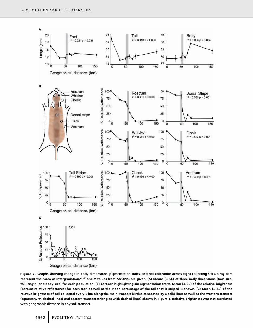
Figure 2. Graphs showing change in body dimensions, pigmentation traits, and soil coloration across eight collecting sites. Gray bars

represent the “area of intergradation.” r2 and P-values from ANOVAs are given. (A) Means (± SE) of three body dimensions (foot size,

tail length, and body size) for each population. (B) Cartoon highlighting six pigmentation traits. Mean (± SE) of the relative brightness

(percent relative reflectance) for each trait as well as the mean percentage of the tail that is striped is shown. (C) Mean (± SE) of the

relative brightness of soil collected every 8 km along the main transect (circles connected by a solid line) as well as the western transect

(squares with dashed lines) and eastern transect (triangles with dashed lines) shown in Figure 1. Relative brightness was not correlated

with geographic distance in any soil transect.



Table 2. Pairwise estimates of population structure based on

eight microsatellite markers surveyed in eight populations. Esti-

mates of FST between sites (below the diagonal) and ML estimates

of the effective number of migrants (Nm; above the diagonal). Es-

timates representing neighboring populations are in bold.

WP CL RL IN CH DP GR AB

WP – 2.41 1.92 2.12 2.27 2.19 1.84 3.45CL 0.170 – 1.62 1.74 1.12 1.20 3.48 2.98RL 0.132 0.084∗ – 5.80 1.48 1.63 5.47 8.56IN 0.085 0.069∗ 0.070 – 3.25 2.03 3.51 3.74CH 0.152 0.067∗ 0.112 0.035 – 6.75 2.52 2.70DP 0.134 0.019 0.122 0.051 0.025 – 4.31 4.68GR 0.118 0.020∗ 0.061∗ 0.030 0.016 0.022 – 3.34

AB 0.371 0.106 0.188 0.153 0.163 0.141 0.105 –

∗F ST values statistically indistinguishable from zero (P < 0.05).

AB; FST = 0.371) that are separated by 155 km. Comparisons of

neighboring populations also showed little evidence of genetic

structure: all of the FST estimates were low (FST < 0.1), with the

exception of the two terminal populations and their nearest neigh-

bor (WP-CL, FST = 0.170 and GR-AB, FST = 0.105). In fact,

the estimates of FST between the central populations (IN to CH),

where most of the change in pigmentation occurs, were among the

lowest of all pairwise comparisons. Overall, migration rates (Nm)

were high, reflecting this low level of genetic structure (Table 2).

The estimated number of migrants ranged from 2 to 7 individuals

per generation between neighboring populations.

Figure 3. Graphical display of individual coefficients of membership in subgroups based on multilocus genotypes using the program

STRUCTURE. Each individual is represented by a vertical line, broken into k colored segments proportional to its membership in each of the

k subgroups. Individuals are grouped by collecting site and separated by a vertical bar. (A) Analysis constrained to k = 2 subgroups. (B)

Analysis using the maximum-likelihood estimate of k = 5 subgroups.

We also found high levels of admixture between populations.

When STRUCTURE was constrained to k = 2 (lnP = −7029.5), we

did not find any clustering of genotypes between the two sub-

populations (Fig. 3A). We found, instead, that the most likely

number of populations is 5 (lnP = −6272.9). Most individuals

had equal membership among the clusters, with the exception of

the coastal WP population, where 80% of genotypes from these

samples were assigned to one cluster (Fig. 3B). We averaged the

highest probability of assignment (q) from each individual and

found q = 0.49 ± 0.14. The probability of assigning any individ-

ual to its correct population is thus less than 50%, which again

shows that extensive gene flow has homogenized subpopulations

for these markers.

COMPARING PHENOTYPIC AND GENETIC VARIATION

Using pairwise and partial MCTs, we found a highly signifi-

cant correlation between pigmentation and geographic distance

(Table 3; r2 = 0.574, P < 0.001). There was also a significant

correlation between geographic and genetic distance (P = 0.001),

but when we controlled for genetic distance, the correlation be-

tween pigmentation and geography remained (r2 = 0.528, P =0.002). Moreover, although there was a correlation between pig-

mentation and genetic distance, when we controlled for the effects

of geography, this correlation became nonsignificant. Thus, vari-

ation in pigmentation is best explained by geographic distance,

not genetic distance.



Table 3. Pairwise and partial matrix correspondence tests (MCT)

between genetic distance (pairwise linearized FST), geographic

distance (km) and phenotypic variation (average brightness of

seven pigmentation traits). Parentheses indicate variable whose

effects were controlled for in the partial MCTs. Regression coeffi-

cients (r2) and P-values are given. Significance levels for all com-

parisons were generated from 10,000 permutations.

r2 P-value

FST-Geography 0.666 0.001∗

Pigmentation-Geography 0.574 <0.001∗

Pigmentation-FST 0.298 0.056Pigmentation-Geography_(FST) 0.528 0.002∗

Pigmentation-FST_(Geography) 0.137 0.249

∗P-values significant after Bonferroni correction for multiple tests (P =0.007).

ESTIMATES OF SELECTION

We characterized the center and width of each cline in pigmenta-

tion; these data are shown in Table 4. Although superficially sim-

ilar (Fig. 2), ML estimates of cline centers are statistically hetero-

geneous among traits (χ2 = 45.61, df = 6, P < 0.001). The cline

centers for two facial patterns (whisker and cheek) were 58 km

from the coast and statistically indistinguishable from each other

(χ2 = 0.00, df = 1, P = 1.0). However, these two estimates were

statistically different than cline center estimates for the other five

traits, which were shifted south, 50–54 km from the coast, and

were also statistically indistinguishable from one another (χ2 =4.83, df = 4, P = 0.305). Maximum-likelihood estimates of cline

widths for pigmentation were also variable among traits (χ2 =42.94, df = 6, P < 0.001). Cline widths for cheek, whisker, dorsal

stripe, flank and tail stripe pigmentation were concordant (6 –

11 km; χ2 = 2.808, df = 4, P = 0.590), and these clines were

narrower than those for rostrum and ventrum (> 48 km).

Table 4. Estimates of cline center (km), cline width (km), and selection coefficient for seven pigmentation traits. Maximum-likelihood

curves were fitted to the average relative brightness for each population. Cline center is shown in kilometers from the Gulf Coast.

Trait Center Width Selection coefficient Selection coefficient(±2 logL) (±2 logL) ecotone model1 gradient model1

Rostrum 52 (46–59)3 48 (22–67)5 0.07 (0.11–0.06) 8.5×10−6 (8.8×10−5–3.1×10−6)Whisker 58 (56–63)2 6 (1–17)4 0.21 (0.51–0.12) 0.004 (0.93–0.0009)Cheek 58 (56–60)2 11 (1–17)4 0.15 (0.51–0.12) 0.0007 (0.93–0.0002)Dorsal stripe 54 (52–55)3 6 (1–11)4 0.21 (0.51–0.15) 0.004 (0.93–0.0007)Flank 52 (41–54)3 9 (4–51)4 0.17 (0.25–0.07) 0.001 (0.01–7.0×10−6)Ventrum 50 (44–56)3 60 (44–85)5 0.07 (0.08–0.05) 4.3×10−6 (1.1×10−5–1.5×10−7)Tail stripe 52 (50–53)3 10 (7–20)4 0.16 (0.19–0.11) 0.001 (0.003–0.0001)

1Range of selection estimates are based on the range of cline width estimates (±2 logL).2Cline center estimates that are statistically equivalent for two traits.3Five traits for which cline center estimates are statistically equivalent.4Cline width estimates that are statistically concordant for five traits.5Traits for which width estimates are statistically concordant with each other. Two different cline centers and two separate cline widths were identified.

Using the width of these phenotypic clines, we estimated the

strength of selection acting on each trait (Table 4). Overall, selec-

tion coefficients were higher under the assumptions of the ecotone

model than the gradient model. Whisker and dorsal stripe had the

highest estimates of selection (s = 0.4% or 21%, depending on the

model), whereas the selection estimates for rostrum and ventrum

were lowest (s = 0.0004% or 7%, depending on the model).

VARIATION IN ALLELE FREQUENCY

AT Mc1r AND AGOUTI

We found distinct changes in allele frequency at each SNP in

the two candidate pigmentation genes (Fig. 4). For Mc1r, we

found that the derived “light” Mc1r allele is present in seven of

the eight populations up to a frequency of 0.34. The light allele

was at intermediate frequency in both the dark- and light-colored

terminal populations (AB = 0.13 and WP = 0.31) and absent in

a central population (CH).

For two Agouti SNPs, the change in allele frequency was not

clinal. For one of these, the SNP closest to the coding region (2

kb SNP), the light allele ranged in frequency from 0.71 to 1.00,

reaching the lowest frequencies in the two terminal populations

and fixation in a central population (CH). The light allele of

the Agouti 50 kb SNP was either fixed or at high frequency in all

populations, with the lowest frequency found in the GR population

(0.95); therefore this marker was uninformative.

In contrast, for the two other Agouti SNPs (40 and 100 kb),

allele frequencies showed clinal variation. For both of these SNPs,

the derived light allele was fixed in the three southernmost popula-

tions, then the light allele began to decrease in frequency starting

in the central IN population, and, finally the light allele showed

its lowest frequency in the northernmost population (0.62 for both

SNPs). This pattern was most striking for the Agouti 40 kb SNP.

Moreover, using ANALYSE to fit a cline to the mean light allele

frequency, we found that estimates of cline center and width for



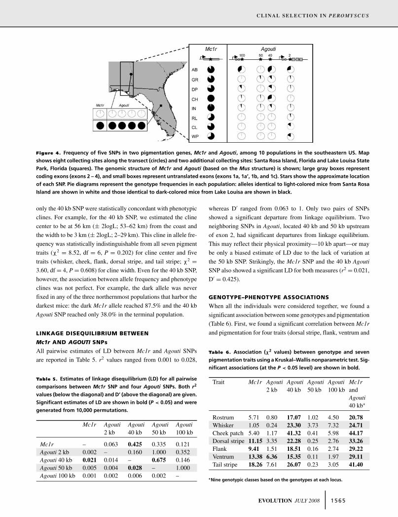
Figure 4. Frequency of five SNPs in two pigmentation genes, Mc1r and Agouti, among 10 populations in the southeastern US. Map

shows eight collecting sites along the transect (circles) and two additional collecting sites: Santa Rosa Island, Florida and Lake Louisa State

Park, Florida (squares). The genomic structure of Mc1r and Agouti (based on the Mus structure) is shown; large gray boxes represent

coding exons (exons 2 – 4), and small boxes represent untranslated exons (exons 1a, 1a’, 1b, and 1c). Stars show the approximate location

of each SNP. Pie diagrams represent the genotype frequencies in each population: alleles identical to light-colored mice from Santa Rosa

Island are shown in white and those identical to dark-colored mice from Lake Louisa are shown in black.

only the 40 kb SNP were statistically concordant with phenotypic

clines. For example, for the 40 kb SNP, we estimated the cline

center to be at 56 km (± 2logL; 53–62 km) from the coast and

the width to be 3 km (± 2logL; 2–29 km). This cline in allele fre-

quency was statistically indistinguishable from all seven pigment

traits (χ2 = 8.52, df = 6, P = 0.202) for cline center and five

traits (whisker, cheek, flank, dorsal stripe, and tail stripe; χ2 =3.60, df = 4, P = 0.608) for cline width. Even for the 40 kb SNP,

however, the association between allele frequency and phenotype

clines was not perfect. For example, the dark allele was never

fixed in any of the three northernmost populations that harbor the

darkest mice: the dark Mc1r allele reached 87.5% and the 40 kb

Agouti SNP reached only 38.0% in the terminal population.

LINKAGE DISEQUILIBRIUM BETWEEN

Mc1r AND AGOUTI SNPs

All pairwise estimates of LD between Mc1r and Agouti SNPs

are reported in Table 5. r2 values ranged from 0.001 to 0.028,

Table 5. Estimates of linkage disequilibrium (LD) for all pairwise

comparisons between Mc1r SNP and four Agouti SNPs. Both r2

values (below the diagonal) and D’ (above the diagonal) are given.

Significant estimates of LD are shown in bold (P < 0.05) and were

generated from 10,000 permutations.

Mc1r Agouti Agouti Agouti Agouti2 kb 40 kb 50 kb 100 kb

Mc1r – 0.063 0.425 0.335 0.121Agouti 2 kb 0.002 – 0.160 1.000 0.352Agouti 40 kb 0.021 0.014 – 0.675 0.146Agouti 50 kb 0.005 0.004 0.028 – 1.000Agouti 100 kb 0.001 0.002 0.006 0.002 –

whereas D′ ranged from 0.063 to 1. Only two pairs of SNPs

showed a significant departure from linkage equilibrium. Two

neighboring SNPs in Agouti, located 40 kb and 50 kb upstream

of exon 2, had significant departures from linkage equilibrium.

This may reflect their physical proximity—10 kb apart—or may

be only a biased estimate of LD due to the lack of variation at

the 50 kb SNP. Strikingly, the Mc1r SNP and the 40 kb Agouti

SNP also showed a significant LD for both measures (r2 = 0.021,

D′ = 0.425).

GENOTYPE–PHENOTYPE ASSOCIATIONS

When all the individuals were considered together, we found a

significant association between some genotypes and pigmentation

(Table 6). First, we found a significant correlation between Mc1r

and pigmentation for four traits (dorsal stripe, flank, ventrum and

Table 6. Association (χ2 values) between genotype and seven

pigmentation traits using a Kruskal–Wallis nonparametric test. Sig-

nificant associations (at the P < 0.05 level) are shown in bold.

Trait Mc1r Agouti Agouti Agouti Agouti Mc1r2 kb 40 kb 50 kb 100 kb and

Agouti40 kb∗

Rostrum 5.71 0.80 17.07 1.02 4.50 20.78

Whisker 1.05 0.24 23.30 3.73 7.32 24.71

Cheek patch 5.40 1.17 41.32 0.41 5.98 44.17

Dorsal stripe 11.15 3.35 22.28 0.25 2.76 33.26

Flank 9.41 1.51 18.51 0.16 2.74 29.22

Ventrum 13.38 6.36 15.35 0.11 1.97 29.11

Tail stripe 18.26 7.61 26.07 0.23 3.05 41.40

∗Nine genotypic classes based on the genotypes at each locus.



tail stripe). For Agouti, we found no association between either the

50 kb or 100 kb SNP and any pigmentation trait. The Agouti 2 kb

SNP showed an association with only ventrum pigment. Most no-

tably, we found the Agouti 40 kb SNP was significantly associated

with all seven pigmentation traits. Moreover, when genotypes at

both Mc1r and the Agouti 40 kb SNP were considered together,

there was also a significant association between genotype and all

seven pigmentation traits—this was not true for any of the other

three Agouti SNPs.

DiscussionUsing molecular genetics and modern mathematical analyses, we

show that natural selection is almost certainly responsible for

maintaining variation in pigmentation among the P. polionotus

populations first studied by Francis Sumner nearly a century ago.

Despite an abrupt change in pigmentation traits along the transect,

populations experience high levels of gene flow, an observation

inconsistent with the hypothesis that the phenotypic cline reflects

recent secondary contact between populations that had diverged

in allopatry. Our results instead imply that the distribution of pig-

ment variants is driven by strong environmentally based selection.

Because the mutations responsible for this pigment variation must

also show clinal variation, we were able to identify an upstream

regulatory region of one candidate pigmentation gene, Agouti,

that may contribute to this classic phenotypic cline.

PHENOTYPE AND ENVIRONMENT

Several morphological traits, including pigmentation, differ

among populations in Sumner’s transect. Foot length and tail

length were measurably larger in mice inhabiting the sandy

beaches than in those inhabiting oldfields. These differences may

have evolved in response to differences in soil type: larger feet

and tails may provide greater stability for mice living on loose

beach sand (Sumner 1917; Blair 1950; Hayne 1950). However,

it remains unclear what proportion of the variation is explained

by genetic versus environmental effects: it is possible, although

unlikely, that foot and tail length are developmental rather than

evolutionary responses to particular substrates (e.g., Losos et al.

2000).

The most striking phenotypic variation, however, is in

pigmentation—with the lightest mice inhabiting white sand

beaches. Although a recent study has attributed pigment variation

in beach mice solely to genetic drift (Van Zant and Wooten 2007),

our data, combined with previous studies, strongly suggest that se-

lection for crypsis is the primary mechanism driving the evolution

of these interpopulation differences in pigmentation. Laboratory

crosses clearly show that pigmentation differences among Sum-

ner’s populations are genetically based (Sumner 1930; Bowen

and Dawson 1977). Enclosure experiments also showed that owls

prey on Peromyscus that match their background substrate less of-

ten than more conspicuous mice (Dice 1947; Kaufman 1974a,b).

Finally, the significant positive correlations between soil color

and all seven pigmentation traits are consistent with selection

for camouflage. Nevertheless, the correlation between coat color

and soil color is not perfect: contemporary soil samples decrease

in brightness by more than 50% within the first 10 km from the

coast, whereas most of the variation in mouse pigmentation occurs

roughly 55 km from the coast.

There are several explanations for this discordance between

the clines in soil color and pigmentation traits. First (although

this seems unlikely), increased urbanization and changes in land

use could have altered soil conditions in the time since Sumner’s

study, so that the break in soil color has recently shifted southward.

Asymmetric gene flow can also account for this discordance: light

mice might, for example, disperse farther than dark ones. How-

ever, our genetic data provide no evidence for asymmetric gene

flow between populations. Asymmetric selection may also con-

tribute to the discordance between soil color and pigmentation.

For example, if predators are more efficient at capturing mice on

different backgrounds, this could shift the break in pigmentation

northward from the break in soil color, as is observed. However,

previous ecological-genetic studies suggest that selection may in

fact be stronger against light mice on dark substrate than vice

versa (Hoekstra et al. 2004), a result consistent with predation

experiments on Peromyscus (Dice 1947). A related and more

plausible explanation is that additional environmental factors (in

combination with soil color) impose differential selection on pop-

ulations. The type and density of vegetative cover, for instance,

may also influence predation risks. Although beach populations

are largely devoid of vegetation, more northern populations have

denser and more diverse vegetation. Therefore, selection could be

more intense on all mice on the beach compared to more northern

environments (thus selection against dark mice on beaches would

be stronger than light mice in the mainland), a scenario that could

produce the observed discordance. For now, however, this discor-

dance between environment and pigmentation remains untested

and largely unexplained.

Although we believe that selection is the primary mechanism

of coat color variation among populations, there is an alternative

explanation: the clinal variation resulted from secondary contact

between formerly isolated populations that diverged in pigmenta-

tion while allopatric. Bowen (1968) noted that the area of abrupt

soil change coincided with the highest Pleistocene shoreline, so

that the decrease in water levels could have allowed a divergent

(and light-colored) subspecies to invade the more coastal habi-

tat. However, under the scenario of recent secondary contact, we

expect that all characters (both genetic and phenotypic) would

share a geographic break at the same location. For phenotypic

traits, differentiation in foot size and tail length occurs more than



25 km south of where the change in brightness occurs, a pattern

inconsistent with this expectation. And for neutral genetic mark-

ers, we see very little genetic differentiation among populations.

Most striking is the complete lack of genetic structure among

populations surrounding the Intergrades (IN), where most of the

change in pigmentation occurs. Thus, we see no evidence for

recent admixture of diverged populations, or any contemporary

barriers to gene flow. Both phenotypic data and neutral genetic

markers suggest that clinal variation in pigmentation is best ex-

plained by strong habitat-specific selection.

These data, however, do not rule out the possibility of

older secondary contact between divergent forms and subse-

quently the maintenance of pigmentation differences by habitat-

specific selection. Careful phylogeographic studies may be able

to provide information about the geographic origins of and di-

vergence times between the terminal populations in this cline.

However, even if secondary contact was ancient, we must still

invoke selection to explain the disparity between the geographic

differentiation in color and the geographic uniformity of many

genetic markers.

In either case, selection must be strong to maintain habitat-

specific phenotypes in the face of high levels of gene flow. In

fact, Haldane (1948) estimated that selection coefficients were

around 10 percent. Using statistical cline-fitting methods, we

indeed found that large selection coefficients are necessary to

explain the observed distribution of pigmentation traits. Our esti-

mates calculated with the ecotone model were remarkably similar

in magnitude to those estimated by Haldane. However, a model

assuming a spatial selection gradient also may be appropriate,

because the phenotypic cline widths (> 5 km) are slightly larger

than the estimated dispersal distance of the mice (< 1 km). As ex-

pected, estimates of selection calculated with the gradient model

were lower than those from the ecotone model. It is also impor-

tant to note that mark–recapture studies often underestimate true

dispersal distance (Mallet et al. 1990; McCallum 2000), thus, our

selection estimates may be conservative. Therefore, it is likely

that the true selection estimates fall between these two extremes.

Under both models, our estimates of selection coefficients

are especially high for several traits—whisker, cheek, flank, and

dorsal stripe—perhaps because these traits are the most visible

to predators. Less-visible traits, such as the ventrum, show the

smallest estimates of selection. However, because all pigmenta-

tion traits are phenotypically and genetically correlated (Hoekstra

et al. 2006; Steiner et al. 2007), it is unclear which is or are the

direct target(s) of selection.

ADAPTIVE GENETIC VARIATION

Previous studies identified two genes, Mc1r and Agouti, that ex-

plain most of the variation in pigment between P. polionotus

leucocephalus, the light-colored Santa Rosa Island beach mouse,

and P. p. subgriseus, a dark mainland mouse (Hoekstra et al. 2006;

Steiner et al. 2007). Like leucocephalus, the beach population in

Sumner’s transect (P. p. allophrys) is significantly lighter than any

mainland subspecies. However, there are some differences in col-

oration between beach subspecies: allophyrs has more pigmented

regions and is slightly darker than leucocephalus.

Despite these phenotypic differences, we were surprised that

there was no clinal variation in the frequency of Mc1r alleles.

Instead, one puzzling result emerged: we found the light Mc1r

allele in dark-colored mice (e.g., mice from the northernmost

populations) despite previous experiments showing that the light

Mc1r allele causes light pigmentation (Hoekstra et al. 2006). One

explanation is that the effects of the light Mc1r allele in Sumner’s

populations could be different from that in the populations where it

was first identified (i.e., P. p. leucocephalus) due to differences in

genetic background. For example, previous work showed that the

light Mc1r mutation does not significantly decrease pigmentation

if found on a dark Agouti background (Steiner et al. 2007). Thus,

we hypothesize the dark mice in the northernmost populations

that harbor light Mc1r alleles also have dark Agouti alleles. It is

also possible, of course, that other pigmentation genes could be

responsible for the similar light color phenotype despite similar

selective pressures.

Unlike Mc1r, we did find clinal allelic variation at the Agouti

locus. Two SNPs, 40 and 100 kb, varied significantly with geo-

graphic distance. This suggests that either two different mutations

in the Agouti cis-regulatory region contribute to pigmentation, or

that both SNPs are in LD with the same causal mutation(s). Addi-

tional genotyping at markers between the 40 kb and 100 kb SNPs

will distinguish between these explanations.

Of these two SNPs, the Agouti 40 kb SNP may be closest to

a causal mutation for several reasons. First, the light allele is fixed

in the light-colored southern populations and occurs at lower fre-

quency, although is not absent, in dark northern populations. This

suggests that the 40 kb SNP may be in LD with a causal SNP that is

driving the clinal variation, but that the SNP is still some distance

away from it, leading to an imperfect association. Second, the

center and width of cline in allele frequency for the 40 kb SNP is

statistically indistinguishable from those of several pigmentation

traits. Third, we found a statistical association between genotypes

at this locus and all seven pigmentation phenotypes. Fourth, the

40 kb SNP is in LD with the Mc1r SNP, which is physically lo-

cated on another chromosome, and this pattern is consistent with

expectations based on their known epistatic interaction (Steiner

et al. 2007). This LD reflects a disproportionately high associ-

ation of the light Mc1r allele with the dark Agouti allele in the

northernmost populations, as predicted if these mice are dark-

colored. Moreover, when genotypes at both Mc1r and the Agouti

40 kb SNP are considered together, there is a statistically signif-

icant association between genotype and all seven pigmentation



traits. Additional genotyping at markers around this 40 kb SNP

will help narrow the region with the goal of eventually identify-

ing the causal mutation(s) in this region. These results highlight

the potential use of natural populations, and clinal variation in

particular, for fine-scale mapping of mutations (Stinchcombe and

Hoekstra 2008).

Together, these data raise several possibilities about the ge-

netic bases of Sumner’s classic pigmentation cline. First, either

this Agouti 40 kb mutation—or, more likely, one or more muta-

tions in LD with this mutation—may contribute to pigmentation

differences among populations. Second, it is likely that this muta-

tion(s) interacts epistatically with the Mc1r mutation, producing

the LD observed between these loci. Third, previous studies sug-

gest that pigment variation in these populations results from the

action of several genes—Sumner’s (1930) genetic analyses of

this transect and Bowen and Dawson’s (1977) study of pigment

pattern variation in natural populations each independently esti-

mated that approximately 10 genes underlie differences between

beach and mainland forms. Our approach also may be valuable in

identifying any additional genes that contribute to naturally oc-

curring variation in pigmentation (or other traits). Together, these

data show that natural selection acting on phenotypes produces

allele frequency clines in the underlying genes, thus allowing us

to narrow in on the precise mutations responsible for adaptive

traits.

ACKNOWLEDGMENTSWe thank several colleagues: J. Patton for access to Sumner’s specimens,T. Belfiore for DNA extraction protocols, S. Hoang for field assistance,M. Streisfeld for help with spectrophotometric analysis, and S. Ramdeenfor providing soil samples from the Florida Geological Survey. Mem-bers of the Hoekstra laboratory, J. Coyne, J. Huelsenbeck, J. Kohn, P.Morin, K. Ruegg, and E. Wilson provided helpful discussion, and addi-tional comments from B. Blackman, D. Haig, A. Kaliszewska, M. Patten,J. Stinchcombe, and two anonymous reviewers greatly improved thismanuscript. This work was supported by an American Society of Mam-malogists Grant-in-Aid, a NSF Graduate Research Fellowship and a NSFDissertation Improvement Grant to LMM, and NSF grant (DEB-0344710)to HEH.

LITERATURE CITEDBarton, N. H., and S. J. E. Baird. 1995. Analyse: an application for

analysing hybrid zones. Available at http://www.biology.ed.ac.uk/research/institutes/evolution/software.php, Edinburgh.

Barton, N. H., and K. S. Gale. 1993. Genetic analysis of hybrid zones. Pp.13–45 in R. G. Harrison, ed. Hybrid zones and the evolutionary process.Oxford Univ. Press, Oxford, UK.

Bazykin, A. D. 1969. Hypothetical mechanism of speciation. Evolution23:685–687.

Beerli, P., and J. Felsenstein. 1999. Maximum-likelihood estimation of mi-gration rates and effective population numbers in two populations usinga coalescent approach. Genetics 152:763–773.

Bennett, A. T. D., and I. C. Cuthill. 1994. Ultraviolet vision in birds: what isits function? Vision Res. 34:1471–1478.

Berry, A., and M. Kreitman. 1993. Molecular analysis of an allozyme cline:alcohol dehydrogenase in Drosophila melanogaster on the east coast ofNorth America. Genetics 134:869–893.

Blair, W. F. 1946. An estimate of the total number of beach-mice of thesubspecies Peromyscus polionotus leucocephalus, occupying Santa RosaIsland, Florida. Am. Nat. 80:665–668.

———. 1950. Ecological factors in speciation of Peromyscus. Evolution4:253–275.

———. 1951. Population structure, social behavior, and environmental rela-tions in a natural population of the beach mouse (Peromyscus polionotus

leucocephalus). Contrib. Lab. Vertebrate Biol. Univ. Michigan 48:1–47.

Bonin, A., E. Bellemain, P. B. Eidesen, F. Pompanon, C. Brochman, and P.Taberlet. 2004. How to track and assess genotyping errors in populationgenetics studies. Mol. Ecol. 13:3261–3273.

Bowen, W. W. 1968. Variation and evolution of gulf coast populations of beachmice, Peromyscus polionotus. Bulletin of the Florida State Museum12:1–91.

Bowen, W. W., and W. D. Dawson. 1977. Genetic analysis of coat patternvariation in oldfield mice (Peromyscus polionotus) of western Florida.J. Mammal. 58:521–530.

Bradbury, P. J., Z. Zhang, D. E. Kroon, T. M. Casstevens, Y. Ramdoss, and E. S.Buckler. 2007. TASSEL: software for association mapping of complextraits in diverse samples. Bioinformatics 23:2633–2635.

Caicedo, A. L., J. R. Stinchcombe, K. M. Olsen, J. Schmitt, and M. D. Purug-ganan. 2004. Epistatic interaction between Arabidopsis FRI and FLCflowering time genes generates a latitudinal cline in a life history trait.Proc. Natl. Acad. Sci. USA 101:15670–15675.

Casgrain, P., and P. Legendre. 2001. The R package for multivariate and spatialanalysis. Universite de Montreal, Departement de Sciences Biologiques.

Dice, L. R. 1947. Effectiveness of selection by owls of deermice (Peromyscusmaniculatus) which contrast in color with their background. Contrib.Lab. Vertebrate Biol. Univ. Michigan 34:1–20.

Dobzhansky, T. 1937. Genetics and the origin of species. Columbia Univ.Press, New York.

Eanes, W. F. 1999. Analysis of selection on enzyme polymorphisms. Annu.Rev. Ecol. Syst. 30:301–326.

Edwards, A. 1992. Likelihood. Johns Hopkins Univ. Press, Baltimore, MD.Endler, J. A. 1977. Geographic variation, speciation, and clines. Princeton

Univ. Press, Princeton, NJ.———. 1990. On the measurement and classification of color in studies of

animal color patterns. Biol. J. Linn. Soc. 41:315–352.Evanno, G., S. Regnaut, and J. Goudet. 2005. Detecting the number of clusters

of individuals using the software STRUCTURE: a simulation study. Mol.Ecol. 14:2611–2620.

Ford, E. B. 1954. Problems in the evolution of geographic races. P. 105 in J.Huxley, A. C. Hardy, and E. B. Ford, eds. Evolution as a process. Allenand Unwin, London.

———. 1960. Evolution in process. Pp. 188–189 in S. Tax, ed. Evolutionafter Darwin. Univ. of Chicago, Chicago.

———. 1964. Ecological genetics. Chapman and Hall, London.Fry, J. D., K. Donlon, and M. Saqeikis. 2008. A worldwide polymorphism

in Aldehyde dehydrogenase in Drosophila melanogaster: evidence forselection mediated by dietary ethanol. Evolution 62:66–75.

Haldane, J. B. S. 1948. The theory of a cline. J. Genet. 48:277–284.Hayne, D. 1950. Reliability of laboratory-bred stocks as samples of wild pop-

ulations, as shown in a study of the variation of Peromyscus polionotus

in parts of Florida and Alabama. Contrib. Lab. Vertebrate Biol. Univ.Michigan 46:1–53.

Hedrick, P. W. 1987. Gametic disequilibrium measures: proceed with caution.Genetics 117:331–341.



———. 2006. Genetic polymorphism in heterogeneous environments: the ageof genomics. Annu. Rev. Ecol. Evol. Syst. 37:67–93.

Hoekstra, H. E., K. E. Drumm, and M. W. Nachman. 2004. Ecological geneticsof adaptive color polymorphism in pocket mice: geographic variation inselected and neutral genes. Evolution 58:1329–1341.

Hoekstra, H. E., R. J. Hirschmann, R. A. Bundey, P. A. Insel, and J. P.Crossland. 2006. A single amino acid mutation contributes to adaptivebeach mouse color pattern. Science 313:101–4.

Howell, A. H. 1920. Description of a new species of beach mouse in Florida.J. Mammal. 1:237–240.

Huxley, J. 1943. Evolution: the modern synthesis. Harper and Brothers, NewYork.

Kaufman, D. W. 1974a. Adaptive coloration in Peromyscus polionotus: exper-imental selection by owls. J. Mammal. 55:271–283.

———. 1974b. Differential owl predation on white and agouti Mus musculus.Auk 91:145–150.

Losos, J. B., D. A. Creer, D. Glossip, R. Goellner, A. Hampton, G. Roberts,N. Haskell, P. Taylor, and J. Etting. 2000. Evolutionary implicationsof phenotypic plasticity in the hindlimb of the lizard Anolis sagrei.Evolution 54:301–305.

Mallet, J., N. Barton, G. Lamas M., J. Santisteban C., M. Muedas, and H.Eeley. 1990. Estimates of selection and gene flow from measures of clinewidth and linkage disequilibrium in Heliconius hybrid zones. Genetics124:921–936.

Mayr, E. 1942. Systematics and the origin of species. Columbia Univ. Press,New York City.

———. 1954. Evolution as a process. P. 105 in J. Huxley, A. C. Hardy, andE. B. Ford, eds. Evolution as a process. Allen and Unwin, London.

———. 1963. Animal species and evolution. Belknap Press of Hrvard Univ.Press, Cambridge, MA.

McCallum, H. 2000. Population parameters: estimation for ecological models.Blackwell Publishing, Oxford.

Morin, P. A., K. E. Chambers, C. Boesch, and L. Vigilant. 2001. Quantita-tive polymerase chain reaction analysis of DNA from noninvasive sam-ples for accurate microsatellite genotyping of wild chimpanzees (Pan

troglodytes verus). Mol. Ecol. 10:1835–1844.Mullen, L. M., R. L. Hirschmann, K. L. Prince, T. L. Glenn, M. J. Dewey, and

H. E. Hoekstra. 2006. Sixty polymorphic microsatellite markers for theoldfield mouse developed in Peromyscus polionotus and P. maniculatus.Mol. Ecol. Notes 6:36–40.

Peakall, R., and P. E. Smouse. 2006. GenALEX 6: genetic analysis in Excel.Population genetic software for teaching and research. Mol. Ecol. Notes6:288–295.

Phillips, B. L., S. J. E. Baird, and C. Moritz. 2004. When vicars meet: anarrow contact zone between morphologically cryptic phylogeographiclineages of the rainforest skink, Carlia rubrigularis. Evolution 58:1536–1548.

Pritchard, J. K., M. Stephens, and P. Donnelly. 2000. Inference of populationstructure using multilocus genotype data. Genetics 155:945–959.

Raymond, M., and F. Rousset. 1995. GENEPOP (version 3.4): populationgenetics software for exact tests and ecumenicism. J. Heredity 86:248–249.

Schemske, D. W., and P. Bierzychudek. 2007. Spatial differentiation for flowercolor in the desert annual Linanthus parryae: was Wright right? Evolu-tion 61:2528–43.

Schmidt, P. S., and D. M. Rand. 2001. Adaptive maintenance of geneticpolymorphism in an intertidal barnacle: habitat- and life-stage-specificsurvivorship of MPI genotypes. Evolution 55:1336–1344.

Schneider, S., D. Roessli, and L. Excoffier. 2000. Arlequin ver. 2.000: Asoftware for population genetics data analysis. Univ. of Geneva, GeneticsBiometry Laboratory, Switzerland.

Slatkin, M. 1973. Gene flow and selection in a cline. Genetics 75:733–56.———. 1995. A measure of population subdivision based on microsatellite

allele frequencies. Genetics 139:457–462.Steiner, C. C., J. N. Weber, and H. E. Hoekstra. 2007. Adaptive variation in

beach mice produced by two interacting pigmentation genes. PLoS Biol.5:e219.

Stinchcombe, J. R., and H. E. Hoekstra. 2008. Population genomics and quan-titative genetics: finding the genes underlying ecologically importanttraits. Heredity 100:158–170.

Sumner, F. B. 1917. The role of isolation in the formation of a narrowlylocalized race of deer-mice (Peromyscus). Am. Nat. 51:173–185.

———. 1926. An analysis of geographic variation in mice of the Peromyscuspolionotus group from Florida and Alabama. J. Mammal. 7:149–184.

———. 1929a. The analysis of a concrete case of intergradation between twosubspecies. Proc. Natl. Acad. Sci. USA 15:110–120.

———. 1929b. The analysis of a concrete case of intergradation between twosubspecies. II. additional data and interpretations. Proc. Natl. Acad. Sci.USA 15:481–493.

———. 1930. Genetic and distributional studies of three subspecies of Per-

omyscus. J. Genet. 23:275–376.Swilling, J. W. R., and M. C. Wooten. 2002. Subadult dispersal in a monoga-

mous species: the Alabama Beach Mouse (Peromyscus polionotus am-

mobates). J. Mammal. 83:252–259.Szymura, J. M., and N. H. Barton. 1986. Genetic analysis of a hybrid zone

between the fire-bellied toads, Bombina bombina and B. variegata, nearCracow in southern Poland. Evolution 40:1141–1159.

Taberlet, P., S. Friffin, B. Goossens, S. Questiau, V. Manceau, N. Escaravage,L. Waits, and J. Bouvet. 1996. Reliable genotyping of samples with verylow DNA quantities using PCR. Nucleic Acids Res. 24:3189–3194.

Van Zant, J. L., and M. C. Wooten. 2007. Old mice, young islands and com-peting biogeography hypotheses. Mol. Ecol. 16:5070–5083.

Associate Editor: J. Feder



Supplementary MaterialThe following supplementary material is available for this article:

Table S1. Sample size and collection numbers for each population.

Table S2. Morphological variation among populations.

Table S3. Pelage and soil reflectance measurements for each population.

Table S4. Forward and reverse primer and TaqMan probe sequences for three Agouti SNPs.

Table S5. Summary of genetic diversity for each population.

This material is available as part of the online article from:

http://www.blackwell-synergy.com/doi/abs/10.1111/j.1558-5646.2008.00425.x

(This link will take you to the article abstract).

Please note: Blackwell Publishing is not responsible for the content or functionality of any supplementary materials supplied

by the authors. Any queries (other than missing material) should be directed to the corresponding author for the article.


natural selection along an environmental gradient: …

Documents