1

Natural Ventilation in Buildings: Measurement in a Wind Tunnel and Numerical Simulation with Large Eddy Simulation

Yi Jianga, Donald Alexanderb, Huw Jenkinsb, Rob Arthurb, Qingyan Chenc*,

aBuilding Technology Program, Massachusetts Institute of Technology 77 Massachusetts Avenue, Cambridge, MA 02139-4307

bWelsh School of Architecture, Cardiff University, Bute Building, King Edward VII Avenue, Cardiff CF10 3NB, Wales, UK

cSchool of Mechanical Engineering, Purdue University, 1288 Mechanical Engineering Building, West Lafayette, IN 47907-1288

*Phone: (765)496-7562, Fax: (765)496-7534, Email: yanchen@purdue.edu Abstract

Natural ventilation in buildings can create a comfortable and healthy indoor environment, and can save energy compared to mechanical ventilation systems. In building design the prediction of ventilation can be difficult; cases of wind driven single-sided ventilation, where the effects of turbulence dominate, are particularly problematic to simulate. In order to investigate the mechanism of natural ventilation driven by wind force, large eddy simulation (LES) is used. In the meanwhile, detailed airflow fields, such as mean and fluctuating velocity and pressure distribution inside and around building-like models were measured by wind tunnel tests and compared to LES results for model validation. Three ventilation cases; single-sided ventilation with an opening in windward wall, single-sided ventilation with an opening in leeward wall, and cross ventilation, are studied. In the wind tunnel, a laser Doppler anemometry (LDA) was used to provide accurate and detailed velocity data. In LES calculations, two subgrid-scale models, a Smagorinsky subgrid-scale model and a filtered dynamic subgrid-scale model, were used.

The numerical results from LES are in good agreement with the experimental data, in particular with the predicted airflow patterns and velocities around and within, and the surface pressures over, the models. This is considered to establish confidence in the application of the LES methods to the calculation of ventilation in buildings, in particular for single-sided ventilation cases. Keywords: large eddy simulation (LES), Smagorinsky subgrid-scale model, filtered dynamic subgrid-scale model, wind tunnel, laser Doppler anemometer (LDA), cross ventilation, single-sided ventilation 1. Introduction

This paper presents a comparison of wind tunnel and numerical simulations of airflow around, within and through bluff bodies with openings. Such simulations may be carried out to allow study of natural ventilation in buildings.

Natural ventilation replaces indoor air with fresh outdoor air without using mechanical power. Hence, natural ventilation can save energy consumed by the heating, ventilating, and air-conditioning systems in a building if it provides acceptable indoor air quality and thermal comfort levels [1]. In addition, poorly designed or maintained mechanical ventilation systems have been associated with health problems such as sick building syndrome. Natural ventilation

Jiang, Y., Alexander, D., Jenkins, H., Arthur, R., Chen, Q. 2003. “Natural ventilation in buildings: measurement in a wind tunnel and numerical simulation with large eddy simulation,” Journal of Wind Engineering and Industrial Aerodynamics, 91(3), 331-353.

2

therefore appears as a cost-effective and attractive alternative to mechanical ventilation, and therefore attracts considerable interest from building designers. However, while natural ventilation is conceptually simple, its detailed design can be a challenge; the ventilation performance involves the buildings’ form, its surroundings and its climate. This complexity can make difficult the prediction of natural ventilation, and so the development of a successful design.

In a naturally ventilated building, air is driven in and out due to pressure differences produced by wind or buoyancy forces. Design for buoyancy is relatively straightforward, and indeed most natural ventilation systems are designed for this force alone. However wind forces are not always beneficial to a ventilation system, and performance can suffer if it is not taken into consideration [2]. This paper is concerned with natural ventilation caused by wind forces. In natural ventilation systems there are two major design foundations; cross ventilation and single-sided ventilation. Cross ventilation provides multiple openings on different facades of a building. The action of any wind will then generate pressure differences between those openings and so promote a robust airflow through an internal space. Cross ventilation is thus the design type of choice, however there are many instances, such as in small cellular offices within a large building, where there may be only one external facade. In those cases single-sided ventilation must be used. In these systems, wind driven ventilation flow is dominated by the turbulence of the wind, as caused by temporal changes in wind speed and direction, and as generated the building itself and its neighbors. Single-sided ventilation may produce significantly less airflow than cross ventilation, so that the size and placement of openings can be critical in achieving a successful design having adequate and robust ventilation. Therefore to refine such a design, it is necessary to use more detailed prediction methods that can take into account all of the factors affecting natural ventilation of a building, and provide detailed airflow information around and inside the building.

Full-scale measurements for a building site can provide reliable ventilation information, such as ventilation rate and the airflow distributions around and inside a building. Katayama, et al.[3], Dascalaki, et al. [4], and Fernandez and Bailey [5] did full-scale measurements for natural ventilation. However, on-site experiments are time consuming, and the measurement data are normally obtained in only a few points so that they are not easily generalized. Furthermore, the wind varies over time in terms of magnitude and direction. So it is difficult to assess those influences on the ventilation performance of a building.

Wind tunnel tests are often used to study natural ventilation. In the wind tunnel, the incoming wind speed and direction are controlled, and small-scale models are used to simulate naturally ventilated buildings. Murakami et al. [6] measured velocity, pressure and ventilation rate in a wind tunnel to analyze the characteristics of cross ventilation. Choiniere and Munroe [7] used smoke to visualize airflow pattern in single-sided situations with different wind directions. However, the measurement data from those wind tunnels are still limited to a few points. Furthermore, the instrumentation used for the velocity measurement [6] can disturb flow patterns and lead to accuracy problems. More commonly wind tunnel measurements of mean surface pressure at openings are often used to provide boundary condition data for numerical calculation of ventilation networks. However these measurements and simulations often neglect turbulence so underestimate or ignore the effect of single-sided ventilation.

Computational fluid dynamics (CFD) provides an alternative approach to calculate ventilation rate and detailed airflow distributions in and around buildings. CFD is becoming popular due to its informative results and low labor and equipment costs, as a result of the

3

development in turbulence modeling and in computer speed and capacity. With these improvements it is becoming feasible to model a domain containing the building, its surroundings and its interior spaces. However the applicability of CFD methods to building natural ventilation problems is not yet fully proven.

In recent years, one of the CFD methods, large eddy simulation (LES) has been successfully applied to several airflows related to buildings [8-10]. LES separates flow motions into large eddies and small eddies, computing the large eddies in a three-dimensional and time dependent way while modeling the small eddies with a subgrid-scale model. An alternative CFD method, Reynolds averaged Navier-Stokes (RANS) modeling, may require less computing time than LES, however it has key limitations as follows. First, RANS modeling has been shown to be not able to correctly predict airflow around buildings. Lakehal and Rodi [11] compared the computed results of airflow around a bluff body by using various RANS and LES models. They found that most RANS models had difficulties generating the separation region on the roof, which was observed in the experiment. Furthermore, the RANS models were found to over-predict the recirculation region behind the body. On the other hand, the LES models did not encounter these problems, and their results agreed well with the experimental data. Secondly, natural wind varies in both speed and direction, so that a transient simulation is required to fully describe the flow [12]. Iaccarino and Durbin [13] have successfully used unsteady RANS modeling to study unsteady turbulent flows. With the RANS modeling, a transient simulation would need much more computing time than a steady-state simulation. Therefore, LES, which always perform transient simulations even for a steady-state flow, is not significantly penalized compared to a transient RANS method.

In the study described here, detailed measurements of airflow around and within a simple building-like cubic body were made in a boundary layer wind tunnel. Two-dimensional mean and fluctuating velocity components were captured using Laser Doppler Anemometer (LDA) equipment. Measurement points were arranged in front, inside, and behind the body. These experimental data were used to validate LES subgrid-scale models. Three different natural ventilation cases were studied: single-sided ventilation with an opening in the windward wall, single-sided ventilation with an opening in the leeward wall, and cross ventilation with openings in both windward and leeward walls. 2. Experimental Description

There are known limitations in the physical scale modeling of ventilation flows through openings [14] which restrict the simulation of ventilation in wind tunnel models. Thus to provide a basis for comparison of physical and numerical methods, this study focuses on a small (250 mm cube) building-like body in a highly turbulent airflow. Essentially the numerical method is used to simulate the wind tunnel and cube, rather than a notional real building. Airflow patterns, both mean and fluctuating values, around and through openings will be recorded and compared. It is considered that should the numerical results compare well to the physical model results, then the numerical method can be applied with confidence to simulations of “full-scale” buildings, and the flow patterns used to calculate ventilation effects.

2.1 Facilities

4

The boundary layer wind tunnel at Cardiff University offers a working section of 2.0m × 2.0m in area and 1.0 m in height. A 6.0 m upstream fetch in the tunnel uses a combination of blockages, fences and surfaces roughness (Lego Duplo blocks) to simulate the lower part of an urban atmospheric boundary layer. The maximum wind speed in the tunnel is about 12.0 m/s.

The instrument to measure the velocity distributions around and inside building models is a one-dimensional Laser Doppler Anemometer (LDA) commercially produced by Dantec. This system allows accurate velocity measurement in highly turbulent and recirculating flows without intruding into those flows. The equipment allows a measurement resolution of ±0.05 m/s. The probe is positioned by a computer controlled traversing arm which provides with a resolution of ±0.5 mm vertically and ±1.0 mm horizontally. Seeding for the LDA system was achieved using a fog mist introduced at the inlet of the tunnel.

The velocity measurements were conducted on a grid plane at the center-section of the building. The velocities were measured along 10 vertical lines, and there were 18 measuring points at each line, ranging from 25 mm to 500 mm high from the tunnel floor. Fig. 1 shows the locations of those measuring lines.

Data for several thousands measurements were collected at each grid point to provide both mean and fluctuating velocities. The LDA system available was one-dimensional, so that measurements in the streamwise and vertical directions were required to be taken in separate runs, with the probe repositioned. Tunnel speed was monitored continuously so that the two components could be normalized; the variation in tunnel speed between measurement runs was within 2%. Since the measurement was conducted along the center-section of the building and the model was symmetrical, the velocities along spanwise direction were expected to be close to zero, and were not measured.

In addition to the velocity measurements, mean surface pressures along the center-section of the building surface were measured, using Furness Control differential pressure transducers coupled to Scanivalve port selectors. Pressure measurement accuracy is less than ±1%. Tunnel reference pressure head, as measured by a pitot tube positioned away from flow disturbances caused by the model, was used to calculate a surface pressure coefficient Cp. 2.2 Building Models

Two building-like models were made for the wind tunnel tests. One was a model with only one opening in a wall, and the other one had openings in two opposite walls. To distinguish the impact of the opening location on natural ventilation, the sizes of these two models and the openings were the same. For simplification, the shape of the models was cubic, and the model dimension was 250 mm × 250 mm × 250 mm. The size of each opening was 84 mm × 125 mm (Length × Height), and the thickness of all the walls is 6 mm. For the model with only one opening, the opening could be placed on either the windward direction or the leeward direction. So three cases were conducted:

• Case 1 - single-sided ventilation with an opening in windward wall • Case 2 - single-sided ventilation with an opening in leeward wall • Case 3 - cross ventilation with openings in both windward and leeward walls

As noted previously, the wind tunnel models were intended to be “building-like”, rather than a scale model of a building. Both the sizes of the model, and of the openings, are large to facilitate measurement.

5

The building models were made of transparent Perspex, so as to allow penetration of the LDA beam to the interior. Fig. 2 shows a schematic view of the building model with one opening in the windward wall (Case 1). 3. Numerical Description

This section will briefly discuss the governing equations of LES, the subgrid-scale model used, the numerical scheme employed for solving the equations. The computational domain, meshes and boundary conditions are also discussed. 3.1 Numerical method

By filtering the Navier-Stokes and continuity equations, one would obtain the governing equations for the large-eddy motions as

j

ij

jj

i2

iji

j

i

xτ

xxuν

xp

ρ1)uu(

xtu

∂

∂−

∂∂∂

+∂∂

−=∂∂

+∂

∂

(1)

0xu

i

i =∂∂

(2)

where ui and uj are the components of the velocity vector in the xi and xj direction, respectively. The variables ρ, p, ijτ and ν represent air density, air pressure, sub-grid scale Reynolds stresses, and kinetic viscosity, respectively. The bar represents grid filtering. Note that the subgrid-scale Reynolds stresses, ijτ , in Eq. (1),

jijiij uuuuτ −= (3) are unknown and must be modeled.

The present study used both the Smagorinsky subgrid-scale (SS) model [15] and filtered dynamic subgrid-scale (FDS) model [10] to model the subgrid-scale Reynolds stresses. 3.2 Numerical scheme

With the subgrid-scale model, the current study used the simplified marker and cell method (SMAC) [16] to solve the governing equations of LES. A second-order central differencing scheme was used to discretize the convection terms, and the explicit Adams-Bashforth scheme to discretize the time term in the filtered Navier Stokes equations. Finally, a staggered grid arrangement eliminated a zigzag type of velocity distribution and the need for a pressure boundary condition [17]. The details about the numerical scheme are available in Ref. [12]. 3.3 Numerical domain and boundary conditions

In the experiments, both building models and their openings had the same dimensions, and

they were placed at the same location in the wind tunnel. So in the numerical simulation, the

6

same computational domain, meshes, and boundary conditions were used in all three cases. This investigation set the length of the building model, 250 mm, as a reference length (H). The computational domain had a downstream length of 8H, an upstream length of 4H, a lateral length of 4H on both sides of the building, and a height of 4H. The Reynolds number was 140,000 based on the velocity at the building height in the inlet of the computational domain.

A non-uniform mesh, 100 × 65 × 80, was used in all three cases. Each case would require one-week CPU time on an Alpha workstation. The time step was 4 × 10-4 seconds, and the smallest mesh was 10-2 H, which was close to the building edge. This spacing was two orders higher than the expected Kolmogorov scale, 10-4 H.

The present study used the wall boundary condition provided by Werner and Wengle [18] to simulate the wall effect. When using large eddy simulation to study the airflow around an obstacle, the periodic inflow boundary condition is not suitable due to the limited computational domain [8]. Therefore, it is necessary to generate the inflow boundary conditions. The variation in U with height was set to match that found in the wind tunnel during the tests. Based on the experimental data, the profile of the mean velocity along the streamwise direction, U, follows a logarithmic law, and the mean velocities in the other two directions were zero. We have checked the impacts of the inflow condition with and without adding turbulence fluctuations on the pressure distributions around the body. It was found that the inflow with the turbulence fluctuations added generated better pressure distributions than that without the added turbulence fluctuations. The results suggested that it is better to add the turbulence fluctuations at the inflow. Although the reason for the better results is not clear, it seems to be related to the magnitude of the turbulence time scale. Therefore, turbulence was added to the mean velocity at the inflow: the fluctuations of the inflow velocity in all three directions are generated by superposing random perturbations with an intensity, u′/U, of 10%. 4. Results and Discussions

Study of the ventilation performance in a building needs detailed airflow information around and inside the building. The information includes the velocity and pressure distributions that can be used to determine the ventilation rate. The following sections present both experimental and numerical results for all three ventilation cases. The velocity distributions around and inside the buildings are presented first. Then the pressure distributions along building surfaces are presented. 4.1 Velocity

In all of the three ventilation cases, the mean and fluctuating velocities along the streamwise

and vertical directions were measured along the center-section of the building models. Figs. 3-5 show that the mean velocities computed from LES with the coarse mesh, 100 × 65 × 80, and the results are generally in good agreement with the experimental data. The difference between the experimental data and the LES results is less than 5% in most regions. This indicates that LES can be used to study natural ventilation driven by wind force with acceptable accuracy. However, there also exist some discrepancies between the experimental data and the numerical results. In all three cases, LES under-predicted the mean velocities along steamwise direction, U, in front the building (X = -H) close to the ground. In addition, the computed mean velocities, U, right above the building roof, which was measured only in Case 2 (single-sided ventilation with

7

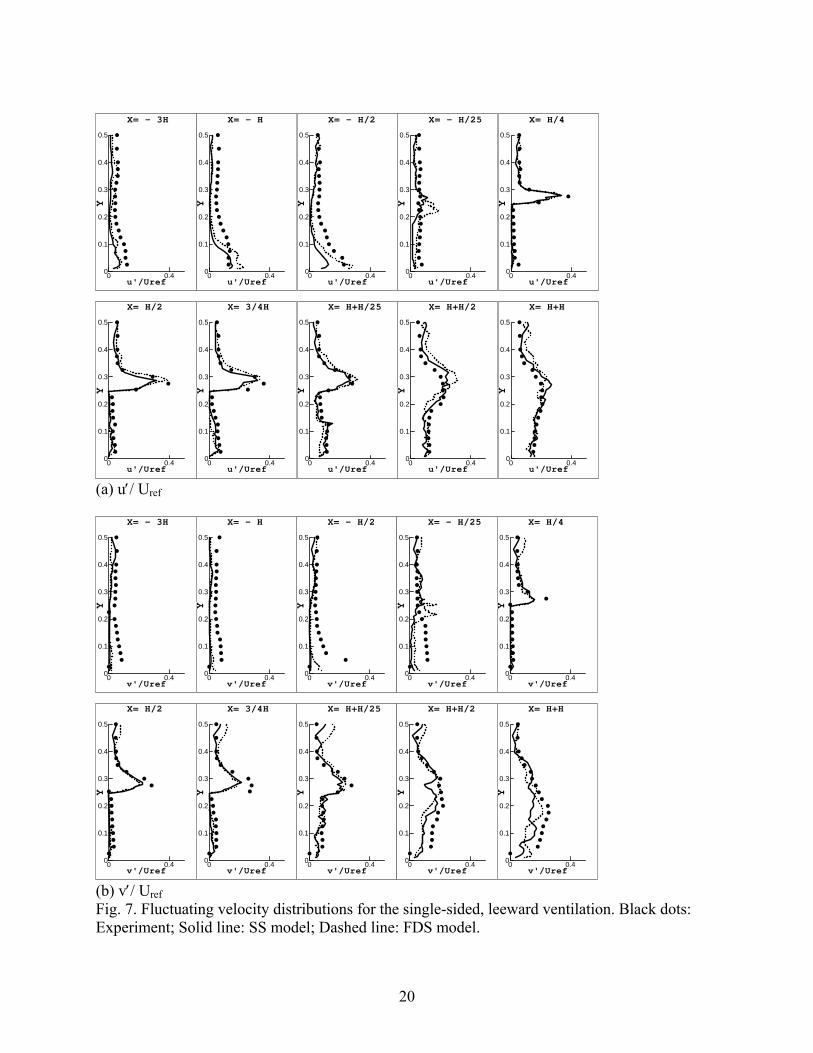
an opening in leeward wall), is 30% larger than the measurement data. This means that the eddy size above the roof is relatively larger in the experiment than that in the simulation. Shah [19] also observed this phenomenon when studying the airflow around a cube with LES. Kato, et al. [20] pointed out that this problem might be attributed to the coarseness of the mesh. Figs. 6-8 show that the fluctuating velocity components computed from LES are also in reasonable agreement with the experimental data.

To investigate whether the grid resolution causes LES to under-predict U in front of the building and over-predict U above the building roof, a finer mesh (140 × 80 × 110) was applied to Case 2 (single-sided ventilation with an opening in leeward wall), where the mean velocities above the building roof were measured in the experiment. Since both of the SS and FDS models provide similar results, only the SS model was used with the fine mesh. Fig. 9 shows the distributions of the mean velocities along steamwise direction, U, in front the building (X = -H), and above the building roof (X = -H/4) with two different grid resolutions. The computed results show that the discrepancies found with the coarse mesh did not occur with the fine mesh, and the fine mesh did provide better agreements with the experimental data. Therefore, the coarseness of the mesh is the reason for the two major discrepancies mentioned above.

However, when we use LES to study natural ventilation, the ventilation rate is the most important parameter that is determined by the flow field distributions at the opening. Since the distributions of the mean and fluctuating velocities close to building openings were correctly predicted with the coarse mesh (Figs. 3-8), the ventilation rate can be calculated correctly with the coarse mesh. It was found that the difference of the computed ventilation rates with these two different grid resolutions is less than 3%. Therefore, the coarse mesh is still adopted in the current investigation.

The results from both subgrid-scale models of LES are almost the same. Shah [19], Rodi, et al. [22], and Jiang and Chen [23] have observed that different subgrid-scale models have similar performance for predicting airflow around a block with high Reynolds numbers. By analyzing the magnitudes of different terms in the momentum equation, Jiang and Chen [23] found that the contribution of the subgrid-scale stresses to the flow is much smaller than that of the resolved stresses in most regions around the block. Therefore, most energy is contained in large eddies, which play a more important role than the small eddies. Since both of the SS and FDS models can directly solve the large-eddy motions, both models are able to provide accurate flow results. In the current study, although the building model is not a block, most of the airflows outside of the building model are fully or nearly fully developed turbulent flows, which are very similar to the airflows around a block. Hence, the computational results from the two subgrid-scale models are almost the same in most of the flow domain.

In some low velocity regions, such as the indoor airflow in the single-sided ventilation cases, the FDS model is expected to perform better than the SS model [21, 23]. However, in the current study, we did not do this comparison because of two reasons. First of all, some measured interior velocities were as low as 0.05 m/s, which were within the error range. Secondly, the fluctuating velocities in most interior regions were higher than the magnitudes of the mean velocities. So in order to obtain accurate velocity information, large amount of data points would be needed at each measuring position. This could require abundant seeding particles entering the model. But as discussed before, there existed difficulty in seeding the interior of the model due to inactive flow motion inside. Therefore, the comparison of the computed results with measurement data inside the building model is not very meaningful.

8

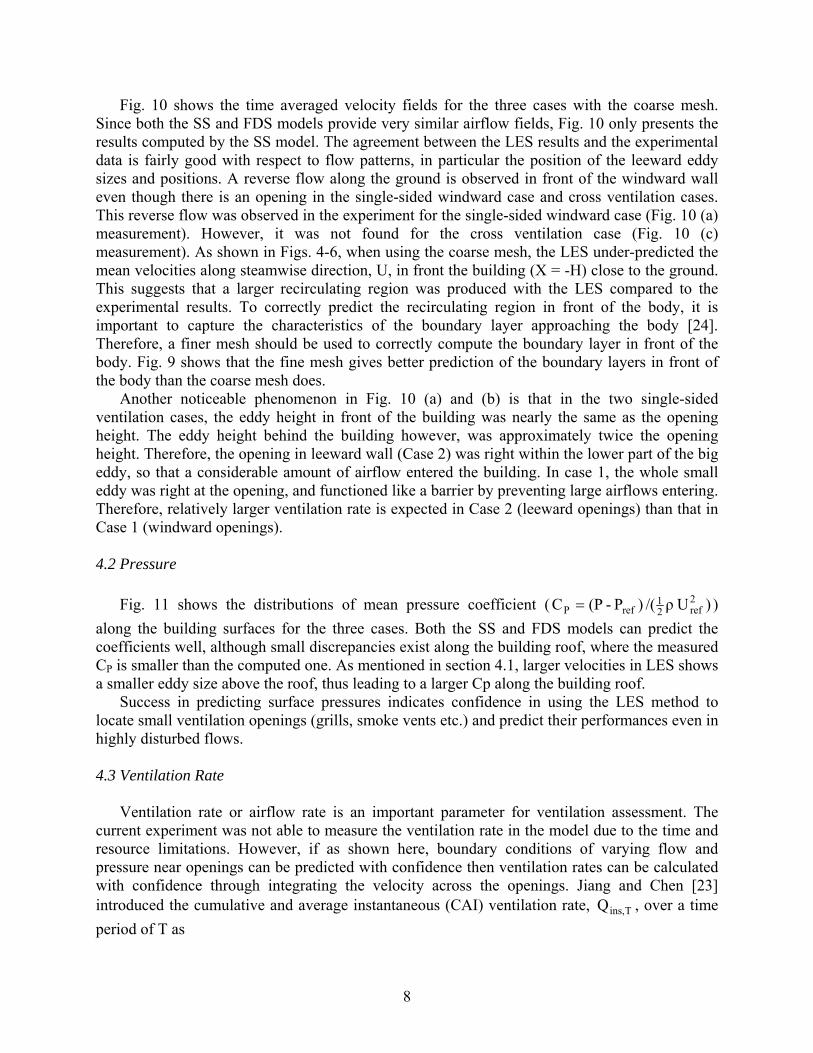
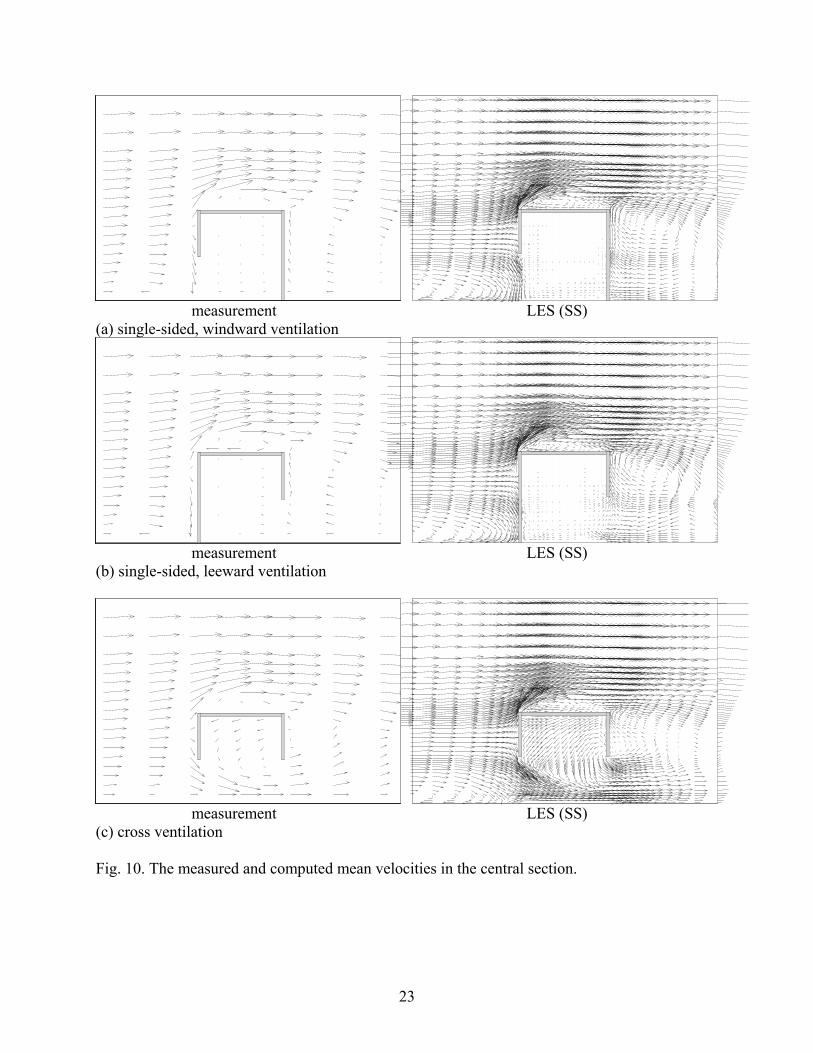
Fig. 10 shows the time averaged velocity fields for the three cases with the coarse mesh. Since both the SS and FDS models provide very similar airflow fields, Fig. 10 only presents the results computed by the SS model. The agreement between the LES results and the experimental data is fairly good with respect to flow patterns, in particular the position of the leeward eddy sizes and positions. A reverse flow along the ground is observed in front of the windward wall even though there is an opening in the single-sided windward case and cross ventilation cases. This reverse flow was observed in the experiment for the single-sided windward case (Fig. 10 (a) measurement). However, it was not found for the cross ventilation case (Fig. 10 (c) measurement). As shown in Figs. 4-6, when using the coarse mesh, the LES under-predicted the mean velocities along steamwise direction, U, in front the building (X = -H) close to the ground. This suggests that a larger recirculating region was produced with the LES compared to the experimental results. To correctly predict the recirculating region in front of the body, it is important to capture the characteristics of the boundary layer approaching the body [24]. Therefore, a finer mesh should be used to correctly compute the boundary layer in front of the body. Fig. 9 shows that the fine mesh gives better prediction of the boundary layers in front of the body than the coarse mesh does.

Another noticeable phenomenon in Fig. 10 (a) and (b) is that in the two single-sided ventilation cases, the eddy height in front of the building was nearly the same as the opening height. The eddy height behind the building however, was approximately twice the opening height. Therefore, the opening in leeward wall (Case 2) was right within the lower part of the big eddy, so that a considerable amount of airflow entered the building. In case 1, the whole small eddy was right at the opening, and functioned like a barrier by preventing large airflows entering. Therefore, relatively larger ventilation rate is expected in Case 2 (leeward openings) than that in Case 1 (windward openings).

4.2 Pressure

Fig. 11 shows the distributions of mean pressure coefficient ( ) Uρ/()P-(PC 2ref2

1refP = )

along the building surfaces for the three cases. Both the SS and FDS models can predict the coefficients well, although small discrepancies exist along the building roof, where the measured CP is smaller than the computed one. As mentioned in section 4.1, larger velocities in LES shows a smaller eddy size above the roof, thus leading to a larger Cp along the building roof.

Success in predicting surface pressures indicates confidence in using the LES method to locate small ventilation openings (grills, smoke vents etc.) and predict their performances even in highly disturbed flows. 4.3 Ventilation Rate

Ventilation rate or airflow rate is an important parameter for ventilation assessment. The current experiment was not able to measure the ventilation rate in the model due to the time and resource limitations. However, if as shown here, boundary conditions of varying flow and pressure near openings can be predicted with confidence then ventilation rates can be calculated with confidence through integrating the velocity across the openings. Jiang and Chen [23] introduced the cumulative and average instantaneous (CAI) ventilation rate, Tins,Q , over a time period of T as

9

∑

∑ ∑ ∑

=

= = =

⋅

= N

1n

n

N

1n

njb

jaj

kb

kakkj

nkj,

Tins,

Δt

Δt)ΔzΔyu(21

Q (4)

where [Δyja, Δyja+1, …, Δyjb] and [Δzka, Δzka+1, …, Δzkb] are the grid sizes in the y and z directions within the opening, respectively; n

kj,u is the instantaneous normal velocity at the opening at time tn, Δtn is the time step size; (tn+1–tn), and N is the total number of the time steps, during which Qins,T is calculated.

Fig. 12 shows the variation of the CAI ventilation rate, Qins,T, over time with both the SS and FDS models in the cross ventilation case. Although the difference of Qins,T is large at the beginning between the two subgrid-scale models, CAI ventilation rate finally reached to 0.0465 m3/s with both models. It suggests that the longer the averaging time is, the more accurate the ventilation rate result is. Therefore, the averaging time should be long enough to give an accurate ventilation rate. Qins,T were also computed for two single-sided ventilation cases.

To compare results against simple design calculations, the cross ventilation rate expected in the model was computed by an empirical method based on Bernoulli equation [4]

prefd ΔCAUCQ = (5) where Cd is the discharge coefficient of the openings, and can be set as 0.78 for a normal large sharp opening [25]. The opening area, A, is computed as:

2out

2in

2 A1

A1

A1

+= (6)

In our case A is 0.0074 m2. The mean pressure coefficient across the openings is about 0.6 for a simple building shape [26], and the reference velocity at the building height is 10 m/s. The corresponding ventilation rate is 0.045 m3/s, which agrees well with the LES result (0.0465 m3/s). This may be because the building model studied is very simple, the two openings are identical, and there are no surrounding buildings around the building model. It is not surprised to see that the empirical model is capable of giving an accurate prediction of the ventilation rate. In a more complex real building design, where surrounding buildings or natural features affect wind flow, and where the configurations of openings are less ideal, the benefits by applying a general numerical method, LES, should become apparent.

An empirical model is also available for single-sided natural ventilation driven by wind [27]. This model calculates the ventilation rate as

Q = 0.025 A U (7) where A is the opening area, and U is the reference velocity. The model determines the ventilation rate as 0.0026 m3/s. Although this empirical model, developed for full-scale buildings, should not be directly compared to our test cube, it is promising that there is an

10

agreement with the LES result (0.0027 m3/s) for the single-sided, windward ventilation case. However, the empirical model does not take the wind direction into account. The LES results indicate that the leeward ventilation case (at 0.0048 m3/s) shows a significantly higher ventilation rate than the windward case.

The larger ventilation rate in Case 2 seems in conflict with common sense: one would expect a higher ventilation rate with a windward opening than that with a leeward opening. However Melaragno [28] has shown that for single-sided ventilation driven by wind force, the mean air velocity inside a building, which is closely correlated to ventilation rate, varies significantly with wind directions. He pointed out that the mean velocity inside a building with one opening in windward wall could be smaller than that in leeward wall. In our wind-tunnel experiment, by visualizing the airflow within the cube, we observed that there existed much stronger air movement within the cell in the leeward opening Case 2 than that in the windward opening Case 1. The LDA measurements also indicate higher velocities and turbulence inside the opening in the leeward case. Table 1 gives the ventilation rates computed by LES and empirical methods in three cases.

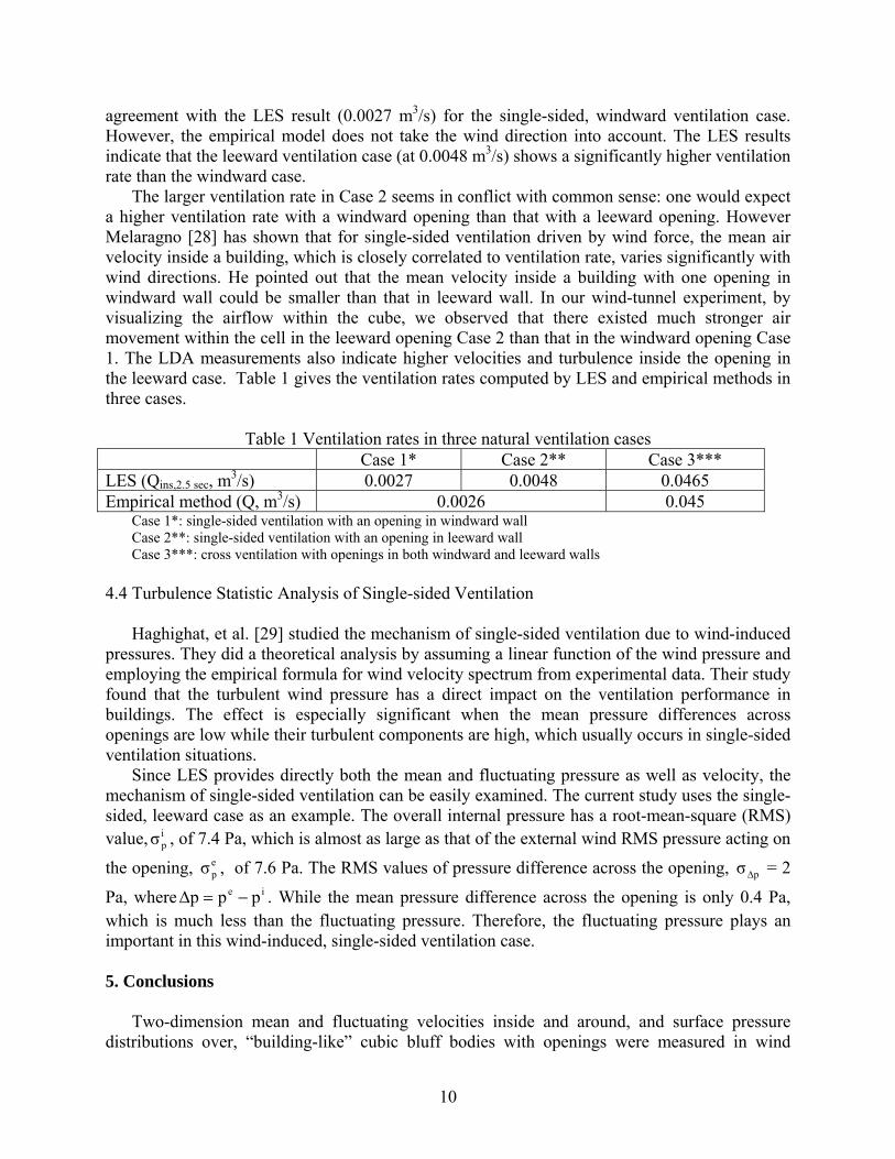
Table 1 Ventilation rates in three natural ventilation cases Case 1* Case 2** Case 3*** LES (Qins,2.5 sec, m3/s) 0.0027 0.0048 0.0465 Empirical method (Q, m3/s) 0.0026 0.045

Case 1*: single-sided ventilation with an opening in windward wall Case 2**: single-sided ventilation with an opening in leeward wall Case 3***: cross ventilation with openings in both windward and leeward walls

4.4 Turbulence Statistic Analysis of Single-sided Ventilation

Haghighat, et al. [29] studied the mechanism of single-sided ventilation due to wind-induced pressures. They did a theoretical analysis by assuming a linear function of the wind pressure and employing the empirical formula for wind velocity spectrum from experimental data. Their study found that the turbulent wind pressure has a direct impact on the ventilation performance in buildings. The effect is especially significant when the mean pressure differences across openings are low while their turbulent components are high, which usually occurs in single-sided ventilation situations.

Since LES provides directly both the mean and fluctuating pressure as well as velocity, the mechanism of single-sided ventilation can be easily examined. The current study uses the single-sided, leeward case as an example. The overall internal pressure has a root-mean-square (RMS) value, i

pσ , of 7.4 Pa, which is almost as large as that of the external wind RMS pressure acting on

the opening, epσ , of 7.6 Pa. The RMS values of pressure difference across the opening, pσΔ = 2

Pa, where ie ppp −=Δ . While the mean pressure difference across the opening is only 0.4 Pa, which is much less than the fluctuating pressure. Therefore, the fluctuating pressure plays an important in this wind-induced, single-sided ventilation case. 5. Conclusions

Two-dimension mean and fluctuating velocities inside and around, and surface pressure distributions over, “building-like” cubic bluff bodies with openings were measured in wind

11

tunnel tests. These were compared to results obtained from large eddy simulation (LES) of the same bodies. Three ventilation cases; single-sided ventilation with an opening in windward wall, single-sided ventilation with an opening in leeward wall, and cross ventilation were considered.

The numerical results from LES methods are in good agreement with the experimental data, in the prediction of gross flow patterns, in mean and fluctuating velocities around and within the model, and in surface pressures. There are some discrepancies between LES results and the experimental data that are mainly due to coarseness of the meshes used in the simulations.

While ventilation rates within the model were not measured, it is considered that the demonstrated ability of the LES methods to calculate, with confidence, the flows near and though openings implies that the methods can accurately predict ventilation even for the turbulence dominated single-sided opening cases.

The numerical results by the two subgrid-scale models (a Smagorinsky subgrid-scale (SS) model and a filtered dynamic subgrid-scale (FDS) model) were almost the same. This is because for the airflow around a building under a high wind speed condition, most energy is contained in large eddies. The large eddies therefore play a more important role than the small eddies. Since both the SS and FDS models can directly solve the large-eddy motions, both models are able to provide accurate flow results.

The results from LES enable us to analyze the velocity and pressure fields of complicated turbulence flows in details, and to give a detailed and accurate assessment of the ventilation performance of a building. In particular, it can provide unsteady flow fields, and thus making it possible to simulate unsteady incoming wind conditions and calculate an instantaneous ventilation rate. Furthermore, LES is capable of examining the impacts of fluctuating pressures on the mechanism of ventilation. In the current study, it was found that the fluctuating pressure plays an important in the wind-induced, single-sided ventilation case.

For single-sided ventilation designs, where there are no concrete and reliable empirical models available, the LES method provides a suitable choice for simulation to allow design development and testing.

Acknowledgement

This work is supported by the U.S. National Science Foundation under grant CMS-9877118. We would like to thank Professor Phillips Jones of Cardiff University for his support. References [1] M. Liddament, A guide to energy efficient ventilation, Air Infiltration and Ventilation Center, Coventry, UK (1996). [2] D. Alexander, H. Jenkins, P.Jones, Investigating the effects of wind on natural ventilation design of commercial buildings. Proceedings Sustainable Building, Abingdon Oxfordshire, UK, 5/6 February 1997, 141-148. [3] Katayama T., Tsutsumi J., and Ishii A. Full-scale measurements and wind tunnel tests on cross-ventilation. J. Wind Eng. Ind. Aerodyn. 41-44 (1992) 2553-2562. [4] E. Dascalaki, M. Santamouris, A. Argiriou, C. Helmis, D. Asimakopoulos, K. Papadopoulos and A. Soilemes, Predicting single sided natural ventilation rates in buildings, Solar Energy 55 (5) (1995) 327-341.

12

[5] J. E. Fernandez, and B.J. Bailey, Measurement and prediction of greenhouse ventilation rates, Agricultural and Forest Meteorology, 58 (3-4) (1992) 229-245. [6] S. Murakami, S. Kato, S. Akabayashi, K. Mizutani and Y.D. Kim, Wind tunnel test on velocity-pressure field of cross-ventilation with open windows, ASHRAE Transactions 97 part 1 (1991) 525-538. [7] Y. Choiniere and J.A. Munroe, A wind-tunnel study of wind direction effects on air-flow patterns in naturally ventilated swine buildings, Canadian Agricultural Engineering, 36 (2) (1994) 93-101. [8] S. Murakami, Overview of turbulence models applied in CWE-1997. J. Wind Eng. Ind. Aerodyn. 74-76 (1998) 1-24. [9] S.J. Emmerich and K.B. McGrattan, Application of a large eddy simulation model to study room airflow. ASHRAE Transactions 104 (1998) 1128-1140. [10] W. Zhang, and Q. Chen, Large eddy simulation of indoor airflow with a filtered dynamic subgrid scale model. International J. Heat and Mass Transfer 43 (17) (2000) 3219-3231. [11] D. Lakehal and W. Rodi, Calculation of the flow past a surface-mounted cube with two-layer turbulence models. J. Wind Eng. Ind. Aerodyn. 67/68 (1997) 65-78. [12] Y. Jiang and Q. Chen, Effect of fluctuating wind direction on cross natural ventilation in buildings from large eddy simulation, Building and Environment, 37 (2002) 379-386. [13] G. Iaccarino and P. Durbin, Unsteady 3D RANS simulations using the v2f model, Annual Research Briefs, Center for Turbulent Research (2000) 263-269. [14] D. Etheridge and Nolan, J., Ventilation measurements at model scale in a turbulent flow. Building and Environment, 14 (1979) 53-64 [15] J. Smagorinsky, General circulation experiments with the primitive equations. I. The basic experiment, Monthly Weather Review 91 (1963) 99-164. [16] F.H. Harlow and J.E. Welch, Numerical calculation of time-dependent viscous incompressible flow, Phys. Fluids 8 (12) (1965) 2182-2189. [17] J. D. Anderson Jr., Computational fluid dynamics: the basics with applications, McGraw-Hill, Inc., USA (1995). [18] H. Werner, and H. Wengle, Large eddy simulation of turbulent flow over and around a cube in a plate channel. Eighth Symposium on Turbulent Shear Flows, Technical University Munich, September 9-11, 1991, pp. 155-168. [19] K.B. Shah, Large eddy simulations of flow past a cubic obstacle, Ph.D. dissertation, Department of Mechanical Engineering, Stanford University, (1998). [20] S. Kato, S. Murakami, A. Mochida, S. Akabayashi , and Y. Tominaga, Velocity-pressure field of cross ventilation with open windows analyzed by wind tunnel and numerical simulation, J. Wind Eng. Ind. Aerodyn. 44 (1-3) (1992) 2575-2586. [21] L. Davidson and P. Nielsen, Large eddy simulation of the flow in a three-dimensional ventilation room, 5th International Conference on Air Distribution in Rooms, ROOMVENT’96, July 17-19, 1996. [22] W. Rodi, J.H. Ferziger, M. Breuer and M. Pourquié, Status of large eddy simulation: results of a workshop, J. of Fluids Eng. 119 (1997) 248-262. [23] Y. Jiang and Q. Chen, Study of natural ventilation in buildings by large eddy simulation, J. Wind Eng. Ind. Aerodyn. 89 (13) (2001) 1155-1178. [24] R. Martinuzzi and C. Tropea, The flow around a surface-mounted prismatic obstacle placed in a fully developed channel flow, J. Fluid Eng. 115 (1993) 85-92.

13

[25] M. Santamouris, Natural convection heat and mass transfer through large openings, Internal report, PASCAL Research Program, European Commission DGX11 (1992). [26] D. Etheridge and M. Sandberg, Building ventilation: theory and measurement, John Wiley and Sons, Chichester, England (1996). [27] BS 5925, Code of practice for design of buildings: ventilation principles and designing for natural ventilation, British Standards Institution, London (1980). [28] M. Melaragno, Wind in architectural and environmental design, Van Nostrand Reinhold, New York (1982). [29] F. Haghighat, J. Rao and P. Fazio, The influence of turbulent wind on air change rates ⎯ a modeling approach, Building and Environment, 26 (2) (1991) 95-109.

14

Figure captions Fig. 1. The locations where air velocities were measured (The thick block represents the building model). Fig. 2. A schematic view of the building model in Case 1 (single-sided ventilation with one opening in windward wall). Fig. 3. Mean velocity distributions for the single-sided, windward ventilation. Black dots: Experiment; Solid line: SS model; Dashed line: FDS model.

(a) U/Uref (b) V/ Uref Fig. 4. Mean velocity distributions for the single-sided, leeward ventilation. Black dots: Experiment; Solid line: SS model; Dashed line: FDS model. Fig. 5. Mean velocity distributions for the cross ventilation. Black dots: Experiment; Solid line: SS model; Dashed line: FDS model. Fig. 6. Fluctuating velocity distributions for the single-sided, windward ventilation. Black dots: Experiment; Solid line: SS model; Dashed line: FDS model. (a) u′/ Uref (b) v′/ Uref Fig. 7. Fluctuating velocity distributions for the single-sided, leeward ventilation. Black dots: Experiment; Solid line: SS model; Dashed line: FDS model. Fig. 8. Fluctuating velocity distributions for the cross ventilation. Black dots: Experiment; Solid line: SS model; Dashed line: FDS model. Fig. 9. Mean velocity distributions for the single-sided, leeward ventilation. Black dots: Experiment; Solid line: SS model with coarse mesh; Dashed line: SS model with fine mesh. Fig. 10. The measured and computed mean velocities in the central section.

(a) single-sided, windward ventilation (b) single-sided, leeward ventilation (c) cross ventilation

Fig. 11. The distributions of mean pressure coefficient, CP ( 2ref2

1ref

P UρP-P

C = ), around the building

model. Black dots: Experiment; Solid line: SS model; Dashed line: FDS model. (a) single-sided, windward ventilation (b) single-sided, leeward ventilation

(c) cross ventilation Fig. 12. The variation of the CAI ventilation rate, Qins,T, vs. averaging time with the two subgrid-scale models. Solid line: SS model; Dashed line: FDS model.

15

Fig. 1. The locations where air velocities were measured (The thick block represents the building model). Fig. 2. A schematic view of the building model in Case 1 (single-sided ventilation with one opening in windward wall).

0 H H/2 -H/2 -H -3H H+H/2 H+H

-H/25 H+

H/25

H/4 3H/4

H = 250 mm

83 84

83

125

250

250

Wind Unit: mm

v

u

16

U/Uref

Y

-0.4 0 0.4 0.8 1.20

0.1

0.2

0.3

0.4

0.5

X= - H

U/Uref

Y

-0.4 0 0.4 0.8 1.20

0.1

0.2

0.3

0.4

0.5

X= - H/2

U/Uref

Y

-0.4 0 0.4 0.8 1.20

0.1

0.2

0.3

0.4

0.5

X= - H/25

U/Uref

Y

-0.4 0 0.4 0.8 1.20

0.1

0.2

0.3

0.4

0.5

X= H/4

U/Uref

Y

-0.4 0 0.4 0.8 1.20

0.1

0.2

0.3

0.4

0.5

X= 3/4H

U/Uref

Y

-0.4 0 0.4 0.8 1.20

0.1

0.2

0.3

0.4

0.5

X= H/2

U/Uref

Y

-0.4 0 0.4 0.8 1.20

0.1

0.2

0.3

0.4

0.5

X= H+H/25

U/Uref

Y

-0.4 0 0.4 0.8 1.20

0.1

0.2

0.3

0.4

0.5

X= H+H/2

U/Uref

Y

-0.4 0 0.4 0.8 1.20

0.1

0.2

0.3

0.4

0.5

X= H+H

U/Uref

Y

0 0.4 0.8 1.20

0.1

0.2

0.3

0.4

0.5

X= - 3H

(a) U/Uref

V/Uref

Y

-0.4 0 0.40

0.1

0.2

0.3

0.4

0.5

X= - 3H

V/Uref

Y

-0.4 0 0.40

0.1

0.2

0.3

0.4

0.5

X= H/2

V/Uref

Y

-0.4 0 0.40

0.1

0.2

0.3

0.4

0.5

X= - H

V/Uref

Y

-0.4 0 0.40

0.1

0.2

0.3

0.4

0.5

X= 3/4H

V/Uref

Y

-0.4 0 0.40

0.1

0.2

0.3

0.4

0.5

X= - H/2

V/Uref

Y

-0.4 0 0.40

0.1

0.2

0.3

0.4

0.5

X= H+H/25

V/Uref

Y

-0.4 0 0.4 0.80

0.1

0.2

0.3

0.4

0.5

X= - H/25

V/Uref

Y

-0.4 0 0.40

0.1

0.2

0.3

0.4

0.5

X= H/4

V/Uref

Y

-0.4 0 0.40

0.1

0.2

0.3

0.4

0.5

X= H+H/2

V/Uref

Y

-0.4 0 0.40

0.1

0.2

0.3

0.4

0.5

X= H+H

(b) V/ Uref Fig. 3. Mean velocity distributions for the single-sided, windward ventilation. Black dots: Experiment; Solid line: SS model; Dashed line: FDS model.

17

U/Uref

Y

-0.4 0 0.4 0.8 1.20

0.1

0.2

0.3

0.4

0.5

X= - H

U/Uref

Y

-0.4 0 0.4 0.8 1.20

0.1

0.2

0.3

0.4

0.5

X= - H/2

U/Uref

Y

-0.4 0 0.4 0.8 1.20

0.1

0.2

0.3

0.4

0.5

X= - H/25

U/Uref

Y

-0.4 0 0.4 0.8 1.20

0.1

0.2

0.3

0.4

0.5

X= H/4

U/Uref

Y

-0.4 0 0.4 0.8 1.20

0.1

0.2

0.3

0.4

0.5

X= 3/4H

U/Uref

Y

-0.4 0 0.4 0.8 1.20

0.1

0.2

0.3

0.4

0.5

X= H/2

U/Uref

Y

-0.4 0 0.4 0.8 1.20

0.1

0.2

0.3

0.4

0.5

X= H+H/25

U/Uref

Y

-0.4 0 0.4 0.8 1.20

0.1

0.2

0.3

0.4

0.5

X= H+H/2

U/Uref

Y

-0.4 0 0.4 0.8 1.20

0.1

0.2

0.3

0.4

0.5

X= H+H

U/Uref

Y

0 0.4 0.8 1.20

0.1

0.2

0.3

0.4

0.5

X= - 3H

(a) U/Uref

V/Uref

Y

-0.4 0 0.40

0.1

0.2

0.3

0.4

0.5

X= - 3H

V/Uref

Y

-0.4 0 0.40

0.1

0.2

0.3

0.4

0.5

X= H/2

V/Uref

Y

-0.4 0 0.40

0.1

0.2

0.3

0.4

0.5

X= - H

V/Uref

Y

-0.4 0 0.40

0.1

0.2

0.3

0.4

0.5

X= 3/4H

V/Uref

Y

-0.4 0 0.40

0.1

0.2

0.3

0.4

0.5

X= - H/2

V/Uref

Y

-0.4 0 0.40

0.1

0.2

0.3

0.4

0.5

X= H+H/25

V/Uref

Y

-0.4 0 0.4 0.80

0.1

0.2

0.3

0.4

0.5

X= - H/25

V/Uref

Y

-0.4 0 0.40

0.1

0.2

0.3

0.4

0.5

X= H/4

V/Uref

Y

-0.4 0 0.40

0.1

0.2

0.3

0.4

0.5

X= H+H/2

V/Uref

Y

-0.4 0 0.40

0.1

0.2

0.3

0.4

0.5

X= H+H

(b) V/ Uref Fig. 4. Mean velocity distributions for the single-sided, leeward ventilation. Black dots: Experiment; Solid line: SS model; Dashed line: FDS model.

18

U/Uref

Y

-0.4 0 0.4 0.8 1.20

0.1

0.2

0.3

0.4

0.5

X= - H

U/Uref

Y

-0.4 0 0.4 0.8 1.20

0.1

0.2

0.3

0.4

0.5

X= - H/2

U/Uref

Y

-0.4 0 0.4 0.8 1.20

0.1

0.2

0.3

0.4

0.5

X= - H/25

U/Uref

Y

-0.4 0 0.4 0.8 1.20

0.1

0.2

0.3

0.4

0.5

X= H/4

U/Uref

Y

-0.4 0 0.4 0.8 1.20

0.1

0.2

0.3

0.4

0.5

X= 3/4H

U/Uref

Y

-0.4 0 0.4 0.8 1.20

0.1

0.2

0.3

0.4

0.5

X= H/2

U/Uref

Y

-0.4 0 0.4 0.8 1.20

0.1

0.2

0.3

0.4

0.5

X= H+H/25

U/Uref

Y

-0.4 0 0.4 0.8 1.20

0.1

0.2

0.3

0.4

0.5

X= H+H/2

U/Uref

Y

-0.4 0 0.4 0.8 1.20

0.1

0.2

0.3

0.4

0.5

X= H+H

U/Uref

Y

0 0.4 0.8 1.20

0.1

0.2

0.3

0.4

0.5

X= - 3H

(a) U/Uref

V/Uref

Y

-0.4 0 0.40

0.1

0.2

0.3

0.4

0.5

X= - 3H

V/Uref

Y

-0.4 0 0.40

0.1

0.2

0.3

0.4

0.5

X= H/2

V/Uref

Y

-0.4 0 0.40

0.1

0.2

0.3

0.4

0.5

X= - H

V/Uref

Y

-0.4 0 0.40

0.1

0.2

0.3

0.4

0.5

X= 3/4H

V/Uref

Y

-0.4 0 0.40

0.1

0.2

0.3

0.4

0.5

X= - H/2

V/Uref

Y

-0.4 0 0.40

0.1

0.2

0.3

0.4

0.5

X= H+H/25

V/Uref

Y

-0.4 0 0.4 0.80

0.1

0.2

0.3

0.4

0.5

X= - H/25

V/Uref

Y

-0.4 0 0.40

0.1

0.2

0.3

0.4

0.5

X= H/4

V/Uref

Y

-0.4 0 0.40

0.1

0.2

0.3

0.4

0.5

X= H+H/2

V/Uref

Y

-0.4 0 0.40

0.1

0.2

0.3

0.4

0.5

X= H+H

(b) V/ Uref Fig. 5. Mean velocity distributions for the cross ventilation. Black dots: Experiment; Solid line: SS model; Dashed line: FDS model.

19

u'/Uref

Y

0 0.40

0.1

0.2

0.3

0.4

0.5

X= H/2

u'/Uref

Y

0 0.40

0.1

0.2

0.3

0.4

0.5

X= 3/4H

u'/Uref

Y

0 0.40

0.1

0.2

0.3

0.4

0.5

X= - H

u'/Uref

Y

0 0.40

0.1

0.2

0.3

0.4

0.5

X= - 3H

u'/Uref

Y

0 0.40

0.1

0.2

0.3

0.4

0.5

X= - H/2

u'/Uref

Y

0 0.40

0.1

0.2

0.3

0.4

0.5

X= H+H/25

u'/Uref

Y

0 0.40

0.1

0.2

0.3

0.4

0.5

X= - H/25

u'/Uref

Y

0 0.40

0.1

0.2

0.3

0.4

0.5

X= H+H/2

u'/Uref

Y

0 0.40

0.1

0.2

0.3

0.4

0.5

X= H/4

u'/Uref

Y

0 0.40

0.1

0.2

0.3

0.4

0.5

X= H+H

(a) u′/ Uref

v'/Uref

Y

0 0.40

0.1

0.2

0.3

0.4

0.5

X= - 3H

v'/Uref

Y

0 0.40

0.1

0.2

0.3

0.4

0.5

X= - H

v'/Uref

Y

0 0.40

0.1

0.2

0.3

0.4

0.5

X= - H/2

v'/Uref

Y

0 0.40

0.1

0.2

0.3

0.4

0.5

X= - H/25

v'/Uref

Y

0 0.40

0.1

0.2

0.3

0.4

0.5

X= H/4

v'/Uref

Y

0 0.40

0.1

0.2

0.3

0.4

0.5

X= H/2

v'/Uref

Y

0 0.40

0.1

0.2

0.3

0.4

0.5

X= 3/4H

v'/Uref

Y

0 0.40

0.1

0.2

0.3

0.4

0.5

X= H+H/25

v'/Uref

Y

0 0.40

0.1

0.2

0.3

0.4

0.5

X= H+H/2

v'/Uref

Y

0 0.40

0.1

0.2

0.3

0.4

0.5

X= H+H

(b) v′/ Uref Fig. 6. Fluctuating velocity distributions for the single-sided, windward ventilation. Black dots: Experiment; Solid line: SS model; Dashed line: FDS model.

20

u'/Uref

Y

0 0.40

0.1

0.2

0.3

0.4

0.5

X= H/2

u'/Uref

Y

0 0.40

0.1

0.2

0.3

0.4

0.5

X= 3/4H

u'/Uref

Y

0 0.40

0.1

0.2

0.3

0.4

0.5

X= - H

u'/Uref

Y

0 0.40

0.1

0.2

0.3

0.4

0.5

X= - 3H

u'/Uref

Y

0 0.40

0.1

0.2

0.3

0.4

0.5

X= - H/2

u'/Uref

Y

0 0.40

0.1

0.2

0.3

0.4

0.5

X= H+H/25

u'/Uref

Y

0 0.40

0.1

0.2

0.3

0.4

0.5

X= - H/25

u'/Uref

Y

0 0.40

0.1

0.2

0.3

0.4

0.5

X= H+H/2

u'/Uref

Y

0 0.40

0.1

0.2

0.3

0.4

0.5

X= H/4

u'/Uref

Y

0 0.40

0.1

0.2

0.3

0.4

0.5

X= H+H

(a) u′/ Uref

v'/Uref

Y

0 0.40

0.1

0.2

0.3

0.4

0.5

X= - 3H

v'/Uref

Y

0 0.40

0.1

0.2

0.3

0.4

0.5

X= - H

v'/Uref

Y

0 0.40

0.1

0.2

0.3

0.4

0.5

X= - H/2

v'/Uref

Y

0 0.40

0.1

0.2

0.3

0.4

0.5

X= - H/25

v'/Uref

Y

0 0.40

0.1

0.2

0.3

0.4

0.5

X= H/4

v'/Uref

Y

0 0.40

0.1

0.2

0.3

0.4

0.5

X= H/2

v'/Uref

Y

0 0.40

0.1

0.2

0.3

0.4

0.5

X= 3/4H

v'/Uref

Y

0 0.40

0.1

0.2

0.3

0.4

0.5

X= H+H/25

v'/Uref

Y

0 0.40

0.1

0.2

0.3

0.4

0.5

X= H+H/2

v'/Uref

Y

0 0.40

0.1

0.2

0.3

0.4

0.5

X= H+H

(b) v′/ Uref Fig. 7. Fluctuating velocity distributions for the single-sided, leeward ventilation. Black dots: Experiment; Solid line: SS model; Dashed line: FDS model.

21

u'/Uref

Y

0 0.40

0.1

0.2

0.3

0.4

0.5

X= H/2

u'/Uref

Y

0 0.40

0.1

0.2

0.3

0.4

0.5

X= 3/4H

u'/Uref

Y

0 0.40

0.1

0.2

0.3

0.4

0.5

X= - H

u'/Uref

Y

0 0.40

0.1

0.2

0.3

0.4

0.5

X= - 3H

u'/UrefY

0 0.40

0.1

0.2

0.3

0.4

0.5

X= - H/2

u'/Uref

Y

0 0.40

0.1

0.2

0.3

0.4

0.5

X= H+H/25

u'/Uref

Y

0 0.40

0.1

0.2

0.3

0.4

0.5

X= - H/25

u'/Uref

Y

0 0.40

0.1

0.2

0.3

0.4

0.5

X= H+H/2

u'/Uref

Y

0 0.40

0.1

0.2

0.3

0.4

0.5

X= H/4

u'/Uref

Y

0 0.40

0.1

0.2

0.3

0.4

0.5

X= H+H

(a) u′/ Uref

v'/Uref

Y

0 0.40

0.1

0.2

0.3

0.4

0.5

X= - 3H

v'/Uref

Y

0 0.40

0.1

0.2

0.3

0.4

0.5

X= - H

v'/Uref

Y

0 0.40

0.1

0.2

0.3

0.4

0.5

X= - H/2

v'/Uref

Y

0 0.40

0.1

0.2

0.3

0.4

0.5

X= - H/25

v'/Uref

Y

0 0.40

0.1

0.2

0.3

0.4

0.5

X= H/4

v'/Uref

Y

0 0.40

0.1

0.2

0.3

0.4

0.5

X= H/2

v'/Uref

Y

0 0.40

0.1

0.2

0.3

0.4

0.5

X= 3/4H

v'/Uref

Y

0 0.40

0.1

0.2

0.3

0.4

0.5

X= H+H/25

v'/Uref

Y

0 0.40

0.1

0.2

0.3

0.4

0.5

X= H+H/2

v'/Uref

Y

0 0.40

0.1

0.2

0.3

0.4

0.5

X= H+H

(b) v′/ Uref Fig. 8. Fluctuating velocity distributions for the cross ventilation. Black dots: Experiment; Solid line: SS model; Dashed line: FDS model.

22

U/Uref

Y

-0.4 0 0.4 0.8 1.20

0.1

0.2

0.3

0.4

0.5

X= - H

U/Uref

Y-0.4 0 0.4 0.8 1.20

0.1

0.2

0.3

0.4

0.5

X= H/4

Fig. 9. Mean velocity distributions for the single-sided, leeward ventilation. Black dots: Experiment; Solid line: SS model with coarse mesh; Dashed line: SS model with fine mesh.

23

measurement LES (SS)

(a) single-sided, windward ventilation

measurement LES (SS)

(b) single-sided, leeward ventilation

measurement LES (SS)

(c) cross ventilation Fig. 10. The measured and computed mean velocities in the central section.

24

Cp

-0.8

-0.4

0

Cp-0.8-0.40

Cp00.40.8

(a) single-sided, windward ventilation

Cp00.40.8

Cp-0.8-0.40

Cp

-0.8

-0.4

0

(b) single-sided, leeward ventilation

25

Cp

-0.8

-0.4

0

Cp-0.8-0.40

Cp00.40.8

(c) cross ventilation

Fig. 11. The distributions of mean pressure coefficient, CP ( 2ref2

1ref

P UρP-P

C = ), around the building

model. Black dots: Experiment; Solid line: SS model; Dashed line: FDS model.

Time (sec)0 0.5 1 1.5 2 2.50.044

0.045

0.046

0.047

0.048

0.049

0.05Q (m /s)3

ins,T

Fig. 12. The variation of the CAI ventilation rate, Qins,T, vs. averaging time with the two subgrid-scale models. Solid line: SS model; Dashed line: FDS model.