naval postgraduate school monterey, california · naval postgraduate school monterey, california...
TRANSCRIPT

NAVAL POSTGRADUATE SCHOOLMonterey, California
ELECTEFEB 10 19940
THESISDECISION ANALYSIS APPLIED TO THE
DEPLOYMENT OFMODULARIZED OCEAN BASING SYSTEMS
by
Robert A. Reifenberger
September 1993
Thesis Advisor: Kneale T. Marshall
Approved for public release; Distribution is unlimited.
~ 94-04503 DIMC QUALITY IN8PEC=
111 111111111111 Hill 11111 i l l l lIl iii94209 038
Security Clasification of this page
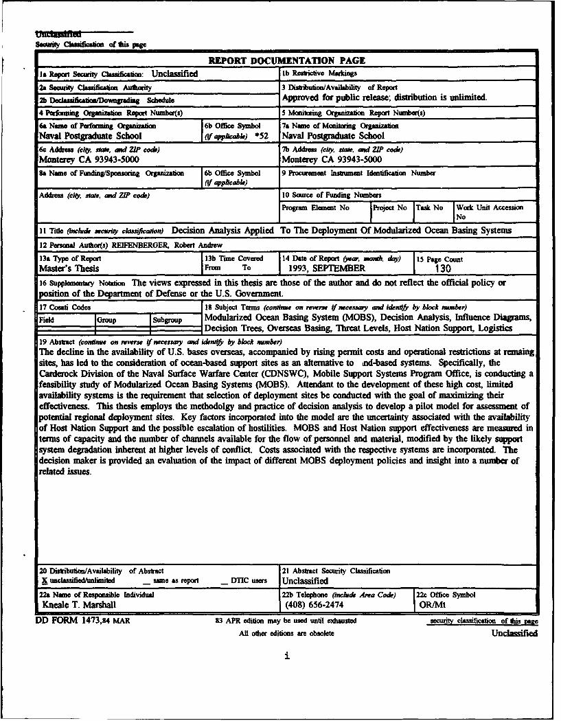
REPORT DOCUMENTATION PAGE
Ia Report Security Clascation: Unclassified lb Restrictive Makings
2a Security Classification Authority 3 Distribution/Availabiiy of Report
2b " Schedule Approved for public release; distribution is unlimited.
4 Pfai Organi n Repo Numbs) 5 Monitoring Orgauizaion Report Number(s)
6& Name of plrforming Orgnization 6b Office Symbol 7a Name of Monitoring OrganizationNaval Postgraduate School Of applicabe) *52 Naval Postgraduate School
6c Address (city state and ZIP code) 7b Address (city, s•te. anud ZIP code)Monterey CA 93943-5000 Monterey CA 93943-5000Sa Name of Funding/Sponsoring Organization 6b Office Symbol 9 Procurment Instrument Identification Number
Address (city, state, and ZIP code) 10 Source of Funding Numbers
Program Element No Project No I Task No EWocrk Unit Accession
11 Title (mclue security clks=catlon) Decision Analysis Applied To The Deployment Of Modularized Ocean Basing Systems12 Personal Author(s) REIFENBERGER, Robert Andrew
13a Type of Report 13b Time Covered 14 Daft of Report (yea, mond ay) 115 Page CountMaster's Thesis IFrom To 1993, SEPTEMBER 1 13016 Supplementmy Notation The views expressed in this thesis are those of the author and do not reflect the official policy orposition of the Department of Defense or the U.S. Government.
17 Cosati Codes 18 Subject Terms (condte on reverse if necessmy and idenify by block number)Field Group Subgroup Modularized Ocean Basing System (MOBS), Decision Analysis, Influence Diagrams,
Fied op Decision Trees, Overseas Basing, Threat Levels, Host Nation Support, Logistics
19 Abstract (cominue on reverse If necessary and identify by block number)The decline in the availability of U.S. bases overseas, accompanied by rising permit costs and operational restrictions at remaingsites, has led to the consideration of ocean-based support sites as an alternative to .nd-based systems. Specifically, theCarderock Division of the Naval Surface Warfare Center (CDNSWC), Mobile Support Systems Program Office, is conducting afeasibility study of Modularized Ocean Basing Systems (MOBS). Attendant to the development of these high cost, limitedavailability systems is the requirement that selection of deployment sites be conducted with the goal of maximizing theireffectiveness. This thesis employs the methodolgy and practice of decision analysis to develop a pilot model for assessment ofpotential regional deployment sites. Key factors incorporated into the model are the uncertainty associated with the availabilityof Host Nation Support and the possible escalation of hostilities. MOBS and Host Nation support effectiveness are measured interms of capacity and the number of channels available for the flow of personnel and material, modified by the likely supportsystem degradation inherent at higher levels of conflict. Costs associated with the respective systems are incorporated. Thedecision maker is provided an evaluation of the impact of different MOBS deployment policies and insight into a number ofrelated issues.
20 Distribution/Availability of Abstract 21 Abstract Security ClassificationX usclassified/unlimited same as report DTIC users Unclassified
22a Name of Responsible Individual 22b Telephone Onclude Area Code) 22c Office SymbolKneale T. Marshall (408) 656-2474 OR/Mt
DD FORM 1473,&4 MAR 83 APR edition may be used until exhausted security classification of this PageAll other editions are obsolete Unclassified
i

Approved for public release; distribution is unlimited.
Decision Analysis Applied to theDeployment of
Modularized Ocean Basing Systems
by
Robert A. Reifenberger
Lieutenant, United States NavyB.S., University of Washington, 1987
Submitted in partial fulfillmentof the requizements for the degree of
MASTER OF SCIENCE IN OPERATIONS RESEARCH
from the
NAVAL POSTGRADUATE SCHOOL
September 1993
Author:
Approved by: UI.
Kneale T. Marshall, Ad
Barbara arsh-eSecond Reader
Peter Purdue, ChairmanDepartment of Operations Research
ii
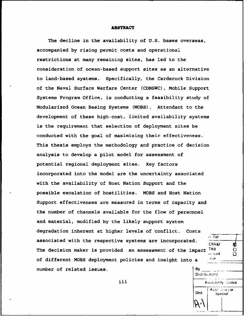
ABSTRACT
The decline in the availability of U.S. bases overseas,
accompanied by rising permit costs and operational
restrictions at many remaining sites, has led to the
consideration of ocean-based support sites as an alternative
to land-based systems. Specifically, the Carderock Division
of the Naval Surface Warfare Center (CDNSWC), Mobile Support
Systems Program Office, is conducting a feasibility study of
Modularized Ocean Basing Systems (MOBS). Attendant to the
development of these high-cost, limited availability systems
is the requirement that selection of deployment sites be
conducted with the goal of maximizing their effectiveness.
This thesis employs the methodology and practice of decision
analysis to develop a pilot model for assessment of
potential regional deployment sites. Key factors
incorporated into the model are the uncertainty associated
with the availability of Host Nation Support and the
possible escalation of hostilities. MOBS and Host Nation
Support effectiveness are measured in terms of capacity and
the number of channels available for the flow of personnel
and material, modified by the likely support system
degradation inherent at higher levels of conflict. Costs, For/ -
associated with the respective systems are incorporated. CRA&I
The decision maker is provided an assessment of the impact TAB 0s;Ced
of different MOBS deployment policies and insight into a __-
number of related issues. ByDistrib;tion I
iii AvaihbNllty CodesAvj. .,d/or
Dist Special

TABLE OF CONTENTS
I. INTRODUCTION ................... 1
A. BACKGROUND ............. .................. 1
B. MOBS: A HISTORICAL PERSPECTIVE. ........ 4
C. INTERNATIONAL LAW OF THE SEA. . ........ 6
D. MOBS DEVELOPMENT MOTIVATION. . ........ 7
1. Overseas Basing Costs. . .......... 8
2. Host Nation Support ....................... 13
E. THESIS GOALS AND OUTLINE ..................... 14
II. MODEL DEVELOPMENT ......... ................ 16
A. PROBLEM STATEMENT ........ ............... 16
B. DECISION MODEL CONTEXT AND OBJECTIVE ..... 16
C. MODELLING APPROACH ....... .............. .. 18
D. DECISION MODEL STRUCTURE ..... ........... .. 19
1. Symbology ........... ................. .. 19
2. Influence Diagrams ...... ............. .. 20
3. Decision Trees ........ ............... .. 21
E. MOBS DECISION MODEL ........ .............. .. 21
1. MOBS Influence Diagram .... ........... .. 22
a. Decision Node ....... ............. .. 22
b. Random Events ....... ............. .. 23
(1) Conflict Level Chance Node . . . . 23
iv

(2) Host Nation Support Chance Node 25
C. Interpretation ...... ............. .. 25
2. Decision Tree ......... ............... .. 30
III. MEASURING RESULTS ......... ................ 31
A. OBJECTIVE AND ATTRIBUTE HIERARCHY ......... .. 31
1. Costs ............. ................... .. 32
2. Effectiveness ......... ............... .. 34
3. Hostile State Offensive Capability . . .. 37
4. The Unifying Equation ..... ........... .. 41
B. TRADE-OFF WEIGHTS ........ ............... .. 41
1. Capacity - Network Value Trade-off (w) . . 42
2. Cost - Effectiveness Trade-off (V) ..... .. 43
IV. CASE STUDY AND ANALYSIS ....... ............. .. 44
A. DECISION MODEL PROCESS FLOW .... .......... .. 44
B. CASE STUDY BACKGROUND ...... ............. .. 44
C. CASE STUDY ........... .................. 48
1. Random Event Node Elements ... ......... .. 49
2. Result Node Elements ...... ............ .. 51
3. Case Study Results ...... ............. .. 55
D. ADDITIONAL CASE STUDIES AND ANALYSIS ..... 62
1. Decision Space Comparison by Hostile State 62
2. Threshold Shift With Network Structure
Change ............ ................... .. 64
3. Shifts in Threshold Values With Increasing T 66
v
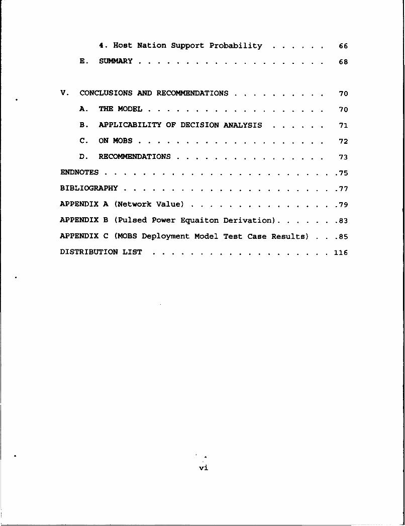
4. Host Nation Support Probability ...... .. 66
E. SUMMARY ............ .................... .. 68
V. CONCLUSIONS AND RECOMMENDATIONS .... .......... .. 70
A. THE MODEL ............ ................... .. 70
B. APPLICABILITY OF DECISION ANALYSIS ...... .. 71
C. ON MOBS ............ .................... .. 72
D. RECOMMENDATIONS ........ ................ .. 73
ENDNOTES .................... ......................... 75
BIBLIOGRAPHY .................. ....................... .77
APPENDIX A (Network Value) ............ ................ 79
APPENDIX B (Pulsed Power Equaiton Derivation) .......... .83
APPENDIX C (MOBS Deployment Model Test Case Results) . .85
DISTRIBUTION LIST ............. ................... .. 116
vi

LIST OF TABLES
Table I MOBS CONFIGURATIONS AND ASSOCIATED COSTS . . .. 12
Table 1I MOBS DATA .............. .................... 47
Table III HOST NATION CARGO CAPACITIES AND NETWORK VALUES . 48
Table IV PROBABILITY OF HOST NATION SUPPORT BY HOST NATION
AND MOBS CONFIGURATION ....... ............. 49
* Table V VULNERABILITY FACTORS ........ .............. 53
Table VI VARIATION IN HOST NATION SUPPORT PROBABILITIES WITH
VARYING NETWORK STRUCTURES ...... ............ 68
vii
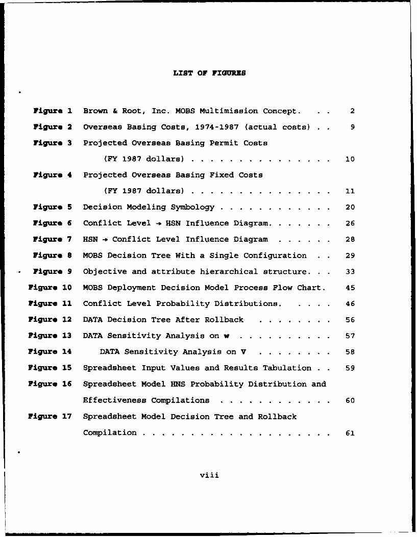
LIST OF FIGURES
Figure I Brown & Root, Inc. MOBS Multimission Concept. 2
Figure 2 Overseas Basing Costs, 1974-1987 (actual costs) 9
Figure 3 Projected Overseas Basing Permit Costs
(FY 1987 dollars) ........ ............... .. 10
Figure 4 Projected Overseas Basing Fixed Costs
(FY 1987 dollars) ........ ............... .. 11
Figure 5 Decision Modeling Symbology ...... ............ .. 20
Figure 6 Conflict Level -* HSN Influence Diagram ......... ... 26
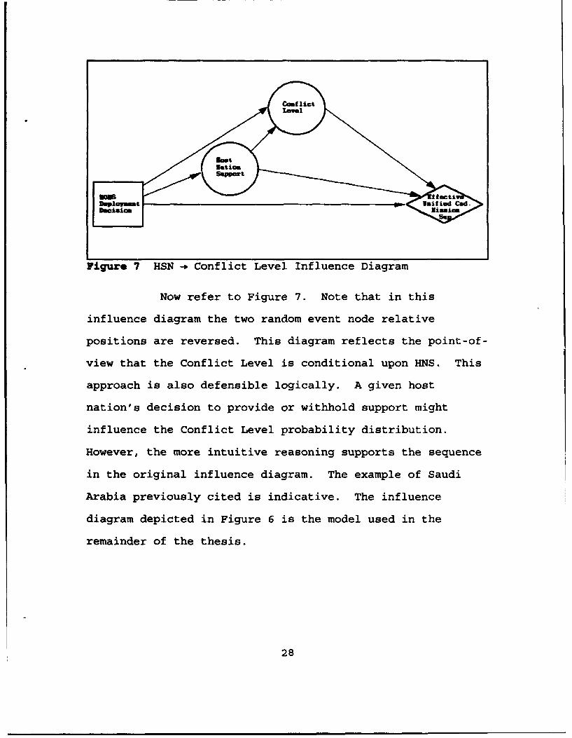
Figure 7 HSN -) Conflict Level Influence Diagram .. ...... .. 28
Figure 8 MOBS Decision Tree With a Single Configuration . 29
Figure 9 Objective and attribute hierarchical structure. . 33
Figure 10 MOBS Deployment Decision Model Process Flow Chart. 45
Figure 11 Conflict Level Probability Distributions . . .. 46
Figure 12 DATA Decision Tree After Rollback ... ........ 56
Figure 13 DATA Sensitivity Analysis on w ... .......... .. 57
Figure 14 DATA Sensitivity Analysis on V .. ........ .. 58
Figure 15 Spreadsheet Input Values and Results Tabulation . 59
Figure 16 Spreadsheet Model HNS Probability Distribution and
Effectiveness Compilations ..... ............ .. 60
Figure 17 Spreadsheet Model Decision Tree and Rollback
Compilation ............ .................... .. 61
viii
Figure 18 Shift In w Threshold With Change In Conflict Level
Distribution ............. ................... .. 63
Figure 19 Shift in V Threshold With Change In Conflict Level
Distribution ............. ................... .. 63
Figure 20 Shift in w Threshold Values With Host Nation
Support Structure Change ..... .............. ... 65
Figure 21 Shift in V Threshold Values With Host Nation
Support Structure Change ..... .............. ... 65
Figure 22 Shift in w Threshold With Decreasing MOBS
Vulnerability ............ ................... .. 67
Figure 23 Shift in V Threshold With Decreasing MOBS
Vulnerability ............ ................... .. 67
ix

IXZCUTIVE SUVflRY
This thesis is an application of probability-based decision
analysis to the deployment of Modularized Ocean Basing
Systems (MOBS), a proposed alternative to foreign territory-based
logistics support sites.
The decline in the availability of U.S. bases overseas,
accompanied by rising permit costs and increasing operational
restrictions at many remaining sites, has led to the assessment
of ocean-based support as an alternative to land-based systems.
The Carderock Division of the Naval Surface Warfare Center,
Mobile Support Systems Program Office, is conducting a
feasibility study of MOBS.
MOBS are composed of semi-submersible platforms similar to
those common in the off-shore oil industry. Construction methods
are based on existing technology and the primary construction
material is prestressed concrete. Experience in the oil industry
and tests conducted to date indicate excellent survivability in
extreme marine environments. A MOBS on the order of six modules
(providing weather deck space of 300' X 3000') would support
C-130 aircraft variants and provide combined liquid and dry cargo
capacities of up to 183,000 short tons. In short, from
production, sustainability, utility standpoints, MOBS is a viable
platform.
It is likely that MOBS would be available in limited numbers
due to high production and deployment costs. The state of the
overseas basing network is such that the number of deployment
x

sites would exceed MOBS availability. Advanced planning on
placement of MOBS is necessitated by MOBS' limited mobility.
These factors indicate the need for a rational and defensible
means of assessing alternative deployment sites.
The advantage of probability-based decision analysis as a
means to fulfill this need is the ability to incorporate
uncertainty, a key factor in the site selection process, along
with strictly deterministic elements into the model.
The uncertainties providing the foundation for the model in
this thesis are those associated with the availability of Host
Nation Support (HNS) and the likely status of hostilities or
conflict level in a given region. Relationships are established
via influence diagrams and decision trees. Results are measured
in terms of cost and effectiveness.
Three scenarios, based on varying conflict level probability
distributions, are employed to exercise the model. Within these
scenarios, three characteristic host nations are described, each
having different capabilities and each varying in the likelihood
of providing those capabilities in support of operations against
a given hostile state.
The decision model is implemented utilizing two different
types of software to demonstrate the portability of the model.
First, the model was constructed in a standard spreadsheet
(Lotus or Quatro Pro). Secondly, commercial decision analysis
software (Decision Analysis by Tree Age) was used.
Analysis of model output provides a description of the
xi

decision space associated with trade-off variables,and the
simplicity of the model allows a rapid assessment of "what if"
excursions. The decision maker is provided a description of the
impact of differing MOBS deployment policies in lieu of point
estimates.
The model, as it has evolved, is envisioned as a
supplementary analysis tool to be used in conjunction with other
methods. Additional levels of complexity can be introduced into
the basic model as desired.
xii
I. INTRODUCTION
A. BACKGROUND
A feasibility study of Modularized Ocean Basing Systems
(MOBS) is being conducted at the Carderock Division of the
Naval Surface Warfare Center (CDNSWC) as a result of the
Mobility Requirements Study and at the direction of
Congress. The thrust of this study is the investigation of
offshore basing systems as a partial solution to problems
associated with forward basing on foreign territory.
Representatives from several affected Department Of
Defense agencies screened a number of contractor-proposed
concepts for MOBS. A Brown & Root, Inc. concept, exploicing
existing semi-submersible oil platform technology, was
deemed the most viable and was selected as the basis for
follow-on study.
Figure 1, on the following page, illustrates the Brown &
Root concept. It consists of semi-submersible platform
modules linked on-site to form an active support base with
many functions inherent in an overseas basing site.
1
.o il
6-4s
F in / muC
Ii--- , Ii-2
i' ' "' '1Il3.I _______
I Ii-il\i
.t [J
II' 3..:11
Figure 1. Brown & Root, Inc. MOBS Multimission Concept.

The scope of possible operations and functions depends
upon size and configuration, which can be tailored for
specific missions. These functions include, but are not
limited to:
* Petroleum, oil, lubricant (POL) storage/transfer
"* Dry and refrigerated stores
"* Ordnance stowage
"* Air strip capable of supporting C-130 variants (C-
130E airlift, KC-130 air tanker, etc.), STOL
(Osprey) and vertical lift aircraft
"* CVBG support
"* Air/surface/subsurface unit repair capabilities
"* Amphibious/Special Warfare operations support
(personnel & material)
"* Ship and aircraft repair capabilities
Pre-stressed concrete is the primary construction
material for MOBS. Comparable existing concrete structures
have survived continuous saltwater immersion well in excess
of 20 years. MOBS would have an intended useful life of up
to 30 years.
Current studies indicate that, even in under what are
defined as "survival conditions" (significant wave height of
50 feet), the MOBS maximum single amplitude roll angle
response is less than 5 degrees, pitch response is less than
10 degrees. A sea base consisting of several modules will
3
have negligible pitch response in sea states less than
survival conditions [Ref. 1].
MOBS exploits existing technology and is composed of
readily available materials. In short, MOBS is a
potentially viable system capable of fulfilling multiple
peace and wartime missions.
B. MOBS: A HISTORICAL PERSPECTIVE
As early as 1928, open-ocean structures were explored as
a means to refuel trans-Atlantic flights (Armstrong
Aerodromes). Artificial island construction was revisited
to a more extensive degree during World War II. The U.S.
Army revived the Armstrong concept and sponsored extensive
analysis and tests including large scale model seakeeping
trials. This effort waned with the advent of long range
fighter and bomber aircraft.
At Winston Churchill's direction, prototypes of tethered
platforms for deployment in the English Channel were
developed. These platforms were envisioned as forward-based
air defense and recovery fields.
Floating logistics centers were created by the U.S. Navy
during WWII by congregating a number of supply, repair ships
and barges at a common anchorage. These units were
connected via a network of causeways, ramps, and
communications links providing what was, in effect, a single
complex.
4

In the early 1960's, the U.S. Air Force sponsored a
study to investigate the feasibility of constructing high
stability seaborne platforms for range instrumentation.
Other projects in the 1960's included a Brown & Root, Inc.,
study into the development of a semi-submersible platform
for support of the MOHOLE program (a project to study the
properties of the Earth's mantle). That concept was the
precursor to that displayed in Figure 1, the design assumed
for this thesis.
From 1963 to 1966, the U.S. Navy sponsored a feasibility
study of a Floating Ocean Research and Development Station
(FORDS) which determined that a semi-submersible
configuration would be the most viable platform. The Rand
Corporation conducted an extensive study in 1969 which drew
on advances in the offshore oil drilling industry to explore
man-made ocean platform concepts.
In 1970, the Naval Postgraduate School was awarded a
contract to conduct studies on operations research aspects
of MOBS. The Naval Civil Engineering Lab (NCEL) released an
exhaustive study in 1971 entitled Mobile Ocean Basing
Systems - A Concrete Concept. The platforms envisioned in
this study were modular semi-submersible platforms combined
to form open ocean multi-functional complexes as large as
1000 feet by 4000 feet. NCEL revised this concept in its
1989 report Modularized Ocean Basing System - A United
States Option in a Strategy of Discriminate Deterrence
5

(Circa 2000). This investigation centered on the
feasibility of floating bases as a practical alternative to
diminishing U.S. foreign basing assets.
This role, that of providing alternatives to overseas
land-bases, continues as the primary motivation for the
current level of interest in MOBS. This aspect is explored
in detail later in this chapter.
C. INTERNATIONAL LAW OF THE SEA
Articles 55-75 of the 1982 United Nations Law of the Sea
(LOS) Convention establish a 200-mile Exclusive Economic
Zone (EEZ) in which a coastal state has both certain
sovereign rights and special rights with respect to
activities undertaken for the economic exploration and
exploitation of the zone. Within the EEZ, a coastal state
has limited jurisdiction with regard to the establishment
and use of artificial islands, installations and structures.
The coastal state has the exclusive right to construct
and regulate the construction, operation, and use of any
artificial islands, and of any installatioi s and structures
for economic purposes, provided that artificial islands,
installations and structures may not be established where
they will interfere with the use of recognized sea lanes
essential to international navigation.
The coastal state has exclusive jurisdiction over such
artificial islands, installations, and structures including
6
jurisdiction with regard to customs, fiscal, health, safety,
and immigration laws and regulations [Ref. 21.
Due to unresolved reservations of the Reagan
Administration, the United States was not a signatory to the
December, 1982 United Nations Convention on the Law of the
Sea. However, in 1983, President Reagan proclaimed a 200-
mile wide EEZ, in terms consistent with the Convention, and
promised that the United States, subject to reciprocity,
would respect similar zones established by other states.
Nearly all provisions of the LOS, particularly those
relating to international navigation and the rights and
duties of coastal states, have become customary
international law and, as such, binding on all states
whether parties to the Convention or not.
The acceptance of the EEZ and associated tenets of the
LOS are the impetus on MOBS peacetime deployment
restrictions to ocean areas beyond the 200-mile limit. As
such, MOBS can be operated free of restrictions as long as
freedom and safety of navigation are not impeded.
D. MOBS DZVELOPMENT MOTIVATION
Two factors concerning the current overseas basing
system compel the development of MOBS: rising costs and
operational freedom.
7
1. Oversea. Basing Costs
The Hudson Institute's U.S. Global Basing Study
categorizes overseas basing costs as either fixe or
p~rmit [Ref. 3]. Fixed costs refer to money that
goes directly to build and maintain the facilities and
installations of a given base. Permit costs refer to monies
paid to several host nations for the "privilege" of building
and maintaining facilities within their territorial borders.
Determining fixed costs is relatively straight-
forward. Permit costs are somewhat less simple to evaluate
because these costs are not strictly labeled as such.
Often, the negotiations for permission to build and maintain
bases on foreign territory include such things as economic
support funding, arms purchasing agreements (Foreign
Military Sales Financing Program), subsidized foreign
military budgets (Military Assistance Program), Status-Of-
Forces Agreements, Peace Keeping Operations, or
International Military Education and Training Programs.
There are two trends associated with the costs of
overseas basing; the first is that both fixed and permit
costs have been rising. The second is that permit costs are
becoming an increasingly larger percentage of the total
overseas basing costs.
Figure 2 depicts these trends which are compiled
from data in the Hudson Institute studies for the years 1974
through 1987 [Ref. 4]. In 1987, combined costs exceeded
8

TAXPAYER COSTS OF OVERSEAS BASING1974-1987
(I)z0
-J 3-J
1974 1975 1976 1977 1970 1979 1980 1981 1982 1963 1984 1905 1986 1987
YEAR
OPERMIT COSTS EMFIXED COSTS -i-TOTAL COSTS
Figure 2 Overseas Basing Costs, 1974-1987 (Actual Costs)
five billion dollars. Projected costs for 1993 are as much
as double that figure.
The Hudson Institute study projected costs through
the year 2000 (in 1987 dollars). Although these studies
were completed prior to the dissolution of the Soviet Union,
the U.S. continues to maintain a policy of power projection
and forward deployment as key components of its National
Strategy. Thus the figures retain a substantial part of
their validity.
9

PROJECTED OVERSEAS BASING PERMIT COSTSFY 1987
4
IiI
z
J 2-J
1969 1999 1990 1991 1992 1993 1994 1995 1996 1997 1998 1999 2000
YEAR
Figure 3 Projected Overseas Basing Permit Costs(FY 1987 dollars)
Projected permit costs (excluding the Philippines)
are shown in Figure 3. The graph shows permit costs
rising 150% by the year 2000.
The Hudson Institute projections for fixed costs
associated with overseas bases includes costs related to the
expansion of bases in Europe and South West Asia (SWA)
anticipated at that time. Events subsequent to the study
may have introduced a degree of error into these figures.
However, they are believed to be fairly accurate and
sufficient for illustrative purposes.
10
PROJECTED FIXED COSTS OF OVERSEAS BASINGFY1987
20
15
z0
J 10-J
E
01967 196 1999 1990 1991 1992 1993 1994 1995 1996 1997 1999 1999 2000
YEAR
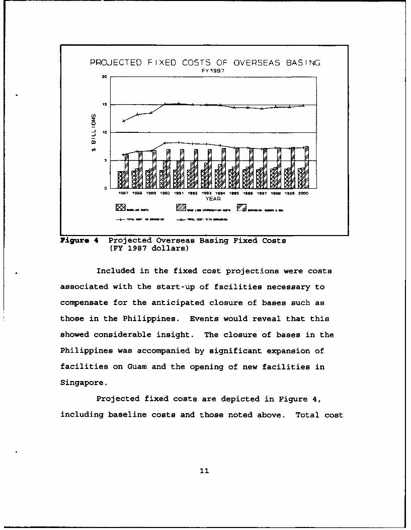
Figure 4 Projected Overseas Basing Fixed Costs(FY 1987 dollars)
Included in the fixed cost projections were costs
associated with the start-up of facilities necessary to
compensate for the anticipated closure of bases such as
those in the Philippines. Events would reveal that this
showed considerable insight. The closure of bases in the
Philippines was accompanied by significant expansion of
facilities on Guam and the opening of new facilities in
Singapore.
Projected fixed costs are depicted in Figure 4,
including baseline costs and those noted above. Total cost
11

Table I MOBS CONFIGURATIONS AND ASSOCIATED COSTS
NO. OF ACQUISITION 0 & XDESIGN MODULUS COST COSTS
MOBS:STOL 3 $0.735 B $ 65 M
MOBS:MULTIMISSION 6 $1.325 B $105 M
lines are shown both including and excluding expansion
costs. Actual costs lie somewhere in-between.
By the year 2000, combined fixed and permit costs
are expected to fall in the range of nine to twelve billion
dollars. An independent NCEL report cites forecasts of
overseas basing costs for 2000 on the order of 11 billion
dollars, 7.5 billion dollars of which would be attributable
to access costs [Ref. 5].
Table 1 shows the estimated acquisition and annual
Operation & Maintenance costs for two variants of the Brown
& Root, Inc. MOBS concept [Ref. 6]. Note that two
multi-mission MOBS could be deployed for less than the cost
of the access rights alone for many of the base sites.
12

2. Host Nation Support
Host nations, fully aware of the value the U.S.
places on overseas bases, come to the access rights
negotiating table with ever-increasing leverage. This
leverage is applied not only to increase the level of
compensation in the variety of forms noted above, but can be
further used to enhance their influence on our national and
international political and economic policies. As we have
experienced in the past, host nations may preclude the use
of territorial facilities or overflight rights for
operations deemed not in their interests.
Other nations, perhaps dealing with internal
dissension concerning U.S. presence on their territory (or,
in the absence of a Soviet threat, simply finding it not in
their interest to maintain a U.S. presence) are considering
the option of eliminating U.S. bases.
MOBS offers an alternative to overseas bases whose
costs exceed their utility or where excessive restrictions
on use are imposed. The mere existence of MOBS would serve
as leverage in our negotiations for existing base sites.
MOBS can provide base facilities in regions where they are
desirable but currently do not exist or could be placed as
necessary to support unilateral operations potentially free
of outside political influence.
Alternatively, MOBS might be perceived as an ideal
platform for combined or United Nations-sanctioned
13
operations. As such, it could provide a stabilizing
influence from international waters without infringing on
regional territories.
Private sector applications, of which there are
many, could proceed concurrently with military deployments
when possible. The two latter options offer the additional
incentive of sharing MOBS development, manufacturing, and
deployment costs. MOBS affords the potential for enhanced
operational latitude while posing interesting questions in a
variety of areas.
E. THESIS GOALS AND OUTLINE
CDNSWC's feasibility study is comprehensive, addressing
functional analysis, systems analysis and operational
requirements, as well as technology and implementation
issues. Wargaming is being employed as an assessment of
MOBS interoperability with existing systems and viability in
selected scenarios.
Not specifically addressed in the CDNSWC study is the
MOBS deployment site selection Drocess. That is, the
establishment of a decision support model providing the
actual Decision Maker (DM) with a structured, concise tool
aimed at exploiting the capabilities of a high-value, scarce
resource to the greatest extent possible.
Establishing a decision support model at this early
stage of MOBS development provides:
14

1. An objective end-use perspective on MOBS.
2. A potential pilot model for use if a MOBS program isimplemented.
3. A means of assessing the efficacy of pursuing MOBSdevelopment (through assessing model output).
The goal of this thesis is to establish such a model.
Chapter II addresses the decision model development.
The objective and attribute hierarchy and measures of
effectiveness are the subjects of Chapter III. Case studies
and analysis follow in Chapter IV. Chapter V presents
conclusions and recommendations.
15

II. MODEL DEVELOPMENT
A. PROBLEM STATEMENT
MOBS, as envisioned, would be a logistics platform
comprising a semi-mobile node in the overseas basing
network. As a logistics platform, there are two key factors
in its employment: configuration and geographic location.
Configuration determines inherent capabilities. Geographic
location determines vulnerability to threats from hostile
states. Both factors determine compatibility with other
bases in the existing logistics network.
The integrity of the mutually supportive logistics
network itself is highly dependent on Host Nation
Support (HNS). The level of HNS may vary with the hostile
state and the type of contingency planned.
Strictly quantifiable aspects of MOBS deployment, those
of the time-distance equation and throughput capacity, are
invariably affected by the uncertainty associated with the
complex political interactions of allied and hostile nations
in conflict.
B. DECISION MODEL CONTEXT AND OBJECTIVE
National Security Strategy, originating at the executive
level, identifies threats and formulates U.S. posture
regarding those threats. Political, economic, and military
16

strategies are developed and implemented, as appropriate, to
mitigate or neutralize both ongoing and emergent threats.
The Chairman, Joint Chiefs of Staff (CJCS) translates
National Military Strategy, as determined by the National
Command Authority, into missions. These missions are
assigned to the Commanders in Chief (CINCs) of operational
commands who are allocated the resources necessary to
accomplish those missions.
The focus of planning at all levels within the
Department of Defense is the support of operational
commanders, particularly the Unified Commanders. This is
the central point of numerous official correspondence,
including the OPNAV Working Draft on Strategic Planning
Guidance and the landmark document ... From The Sea. It is
appropriate that the objective in making the MOBS deployment
decision is Effective Unified Commander Mission SuDport.
The viewpoint of the CINCs provides a regional
perspective ideal for evaluation of potential MOBS
deployment sites as part of the overseas basing structure.
The regional commands applicable to MOBS deployment are the
Atlantic Command, Pacific Command, European Command, and
Central Command. This derives from the fact that MOBS is a
sea-based system. The Decision Maker (DM) is therefore
assumed to exist within the hierarchies of the above
commands.
17
It is further assumed that the information available to
the DM includes the following:
"* Missions assigned
"* A prioritized list of states identified as posing athreat to National Security
"* Resources and capabilities of allies and potentialallies and a reasonable estimate of those of oppositionforces
"* Assessment of the regional political climate.
This information is critical to the development of
probability distributions identified later in this chapter.
Due to its limited mobility, the MOBS deployment site
selection would be based on projected situations and
operations. As discussed in Chapter I, MOBS is a high-
value/limited-availability resource. Its deployment must be
part of the deliberate planning process to realize MOBS full
potential.
C. MODELLING APPROACH
The DM, in this case assumed to be a staff member(s) of
a command noted above, is confronted with the problem of
selecting an "optinmal" MOBS deployment site from a number of
alternatives. Uncertainty regarding the availability of HNS
and the degree of escalation/de-escalation of conflict
(Conflict Level) within a region are underlying determinants
18

of deployment effectiveness. Also uncertain is the effect
of the presence of MOBS itself on these factors.
This uncertainty represents the state of nature, the
uncontrollable factors (from the DM perspective) surrounding
the decision problem. These characteristics define a
classic case for the methodology and practice of Decision
Analysis.
Kirkwood states that,
Decision analysis provides a practical, defensibleapproach to quantitatively analyzing decisions underuncertainty [Ref. 7] .
The components of decision analysis include influence
diagrams, decision trees, subjective or statistical
probability, and a measure of results (value or utility).
The decision analysis methodology employed in this thesis
will be as described in Marshall and Oliver [Ref. 8]
and Chankong and Haimes [Ref. 9].
D. DECISION MODEL STRUCTURE
1. Symbology
Figure 5 displays the symbology, standard in the
literature, used throughout the remainder of this thesis.
The symbology is common to both influence diagrams and
decision trees employed in the modeling process.
19
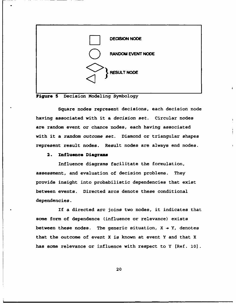
D DECISION NODE
O RANDOM EVENT NODE
<> } RESULT NODE
Figure 5 Decision Modeling Symbology
Square nodes represent decisions, each decision node
having associated with it a decision set. Circular nodes
are random event or chance nodes, each having associated
with it a random outcome set. Diamond or triangular shapes
represent result nodes. Result nodes are always end nodes.
2. Influence Diagrams
Influence diagrams facilitate the formulation,
assessment, and evaluation of decision problems. They
provide insight into probabilistic dependencies that exist
between events. Directed arcs denote these conditional
dependencies.
If a directed arc joins two nodes, it indicates that
some form of dependence (influence or relevance) exists
between these nodes. The generic situation, X -* Y, denotes
that the outcome of event X is known at event Y and that X
has some relevance or influence with respect to Y [Ref. 10].
20

3. Decision Trees
The decision tree evolves from, and is used in
conjunction with, the influence diagram. Decision trees
provide a visual representation of the sequence of decisions
and random events that can occur in all possible scenarios
of the decision problem. Branches are used to denote
possible outcomes of random events or alternatives for a
given decision in the described process.
From any given decision node there will be as many
branches as there are possible decisions. From any given
random event or chance node there will be as many branches
as there are outcomes [Ref. ill.
R. MODS DECISION MODEL
Decision-making models are intended to reduce real world
complexities through a process of abstraction, including
only important elements of the system modeled, to allow the
DM to use the model to concentrate on the important aspects
of the problem at hand. Too much complexity becomes
unmanageable. Too much abstraction does not adequately
reflect the true nature of the decision-making process.
The development of this decision model produced several
generations of influence diagrams. Early variations
resulted in thousands of possible decision tree end nodes.
Through a combination of node synthesis, the elimination of
relatively unimportant elements, and the employment of a
" ~21
iterative design, the resulting model was reduced to four
node sets and generally fewer than 50 result nodes.
The process is illustrated in Chapter IV. The following
sections explain specific model elements.
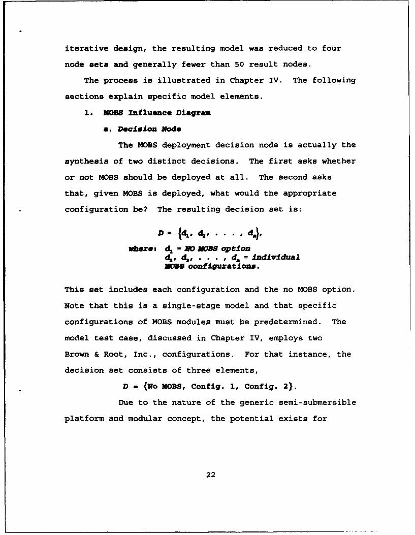
I. MOSS Influence Diagram
a. Decision Node
The MOBS deployment decision node is actually the
synthesis of two distinct decisions. The first asks whether
or not MOBS should be deployed at all. The second asks
that, given MOBS is deployed, what would the appropriate
configuration be? The resulting decision set is:
D = Id,,, d2, I . . 0'd,
where. d, =No MOBS optiond2 , d3,. . . , d, = individualMOBS configuratlons.
This set includes each configuration and the no MOBS option.
Note that this is a single-stage model and that specific
configurations of MOBS modules must be predetermined. The
model test case, discussed in Chapter IV, employs two
Brown & Root, Inc., configurations. For that instance, the
decision set consists of three elements,
D a (No MOBS, Config. 1, Config. 2).
Due to the nature of the generic semi-submersible
platform and modular concept, the potential exists for
22
numerous possible configurations. However, it is assumed
that, due to the high costs involved, only a few general
configurations (two to three) would be applicable in a given
instance, and those configurations are primarily a factor of
the aircraft they are required to support.
b. Random Zventa
As noted previously, several aspects of the
prevailing regional political climate introduce uncertainty
into the decision process. Uncertainty exists as to the
level of conflict likely to evolve in a given set of
circumstances. Uncertainty also exists in regard to the
availability of HNS either from existing overseas bases or
from emergent base sites made available by coalition forces
in support of a given regional contingency.
(1) Conflict Level Chance Node
Execution of U.S. military strategy in a
given region has one of the following consequences:
"* Conflict deterred
"* Status quo maintained
"* Conflict escalates.
Some degree of forward presence is required to carry out
strategy. Forward presence is therefore assumed to be a
baseline in any MOBS deployment candidate location. This
presence is normally maintained either by military forces
23

positioned in countries neighboring hostile states or by
U.S. Naval forces in adjacent seas or both.
By designating presence as a lower bound on
military involvement, a scale can be developed encompassing
the possible consequences of a strategy in a given region:
Level 1. Forward Presence. As described above.Includes, for the purposes of this thesis, militaryinvolvement in drug interdiction operations andhumanitarian relief.
Level 2. Low Intensity Conflict (LIC). A criticalsituation that can be settled (terminated or contained)with a small on-scene combat potential, with or withoutactual exchange of weapons fire. Peacekeeping operationswould fall under this criteria.
Level 3. Leoser Regional Conflict (LRC). Combat power isemployed. The scale is an the order of Grenada orPanama, but not necessarily of short duration.Peacemaking would fell under this criteria.
Level 4. Major Regional Conflict (NRC). Combat power isemployed on a large, sustained, taxing level and employsJoint forces. Examples are Vietnam, the Korean War, andDesert Shield/Desert Storm.
Level 5. War. Assumed to be a major conflict involvingJoint/Allied forces opposing a coalition of enemyforces [Ref. 12].
The resulting random event set is:
C = 1, Level 2, Level 3, Level 4, Level
vheret the letter C denotes a chance node andthe superacript CL denotes Conflict Level.
24

(2) Host Nation Support Chance Node
The integrity of the overseas basing network
is highly dependent on Host Nation Support (HNS). History
has shown that a given host nation may restrict or preclude
the use of its facilities for use in supporting
contingencies deemed not in their best interest. HNS will
depend on the political climate attendent to operations and
the willingness of the Host Nation to permit use of
facilities on its territory in support of that operation.
For example, HNS was invaluable in the
success of Desert Shield/Desert Storm. Conversely, the
absence of HNS greatly complicated U.S. air operations in
Libya.
The disposition of critical host nation
facilities would affect the value of MOBS. Therefore, the
uncertainty associated with HNS is addressed by determining
a distribution for the probability that a critical host
nation will be available to support a contingency against a
given hostile nation. The resulting random event set is
binary:
CAM = {Jloat Nation Suppozt, Absence of Host Nation Supporxt.
c. Interpreztation
Refer to the influence diagram in Figure 6 on the
following page. The MOBS deployment decision is assumed to
25
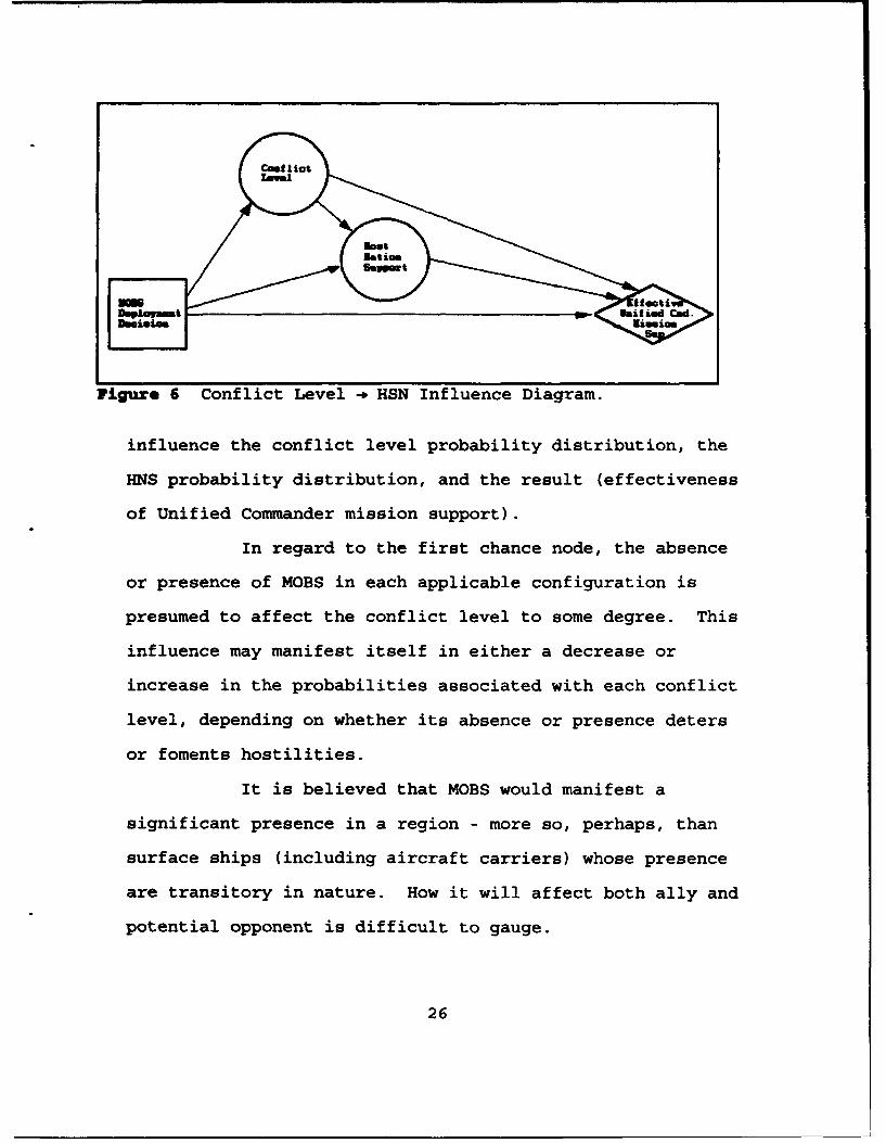
i e. 6 Conflict Level -' HSN Influence Diagram.
influence the conflict level probability distribution, the
HNS probability distribution, and the result (effectiveness
of Unified Commander mission support).
In regard to the first chance node, the absence
or presence of MOBS in each applicable configuration is
presumed to affect the conflict level to some degree. This
influence may manifest itself in either a decrease or
increase in the probabilities associated with each conflict
level, depending on whether its absence or presence deters
or foments hostilities.
It is believed that MOBS would manifest a
significant presence in a region - more so, perhaps, than
surface ships (including aircraft carriers) whose presence
are transitory in nature. How it will affect both ally and
potential opponent is difficult to gauge.
26

It can be seen at the second chance node in
Figure 6 that HNS is impacted by both the decision and the
conflict level. This assumption is both intuitive and
defensible.
It is reasonable to believe that the presence of
a MOBS in a region will influence a Host Nation's
willingness to permit access. MOBS could be perceived as
representing a facility which diminishes the need for use of
terrestrial-based U.S. forces on their soil or,
alternatively, even as a threat to themselves (if the U.S.
is acting unilaterally).
Historically, host nations have been willing to
support a presence or peacekeeping forces (Levels 1 & 2) but
balk at supporting increasing levels of operations.
Conversely, as in the case of Saudi Arabia during Desert
Shield/Storm, a prospective host nation may be unwilling to
permit a foreign presence on their territory until their
sovereignty is threatened at the MRC or higher conflict
level. The conditional probabilities at the two respective
chance nodes are:
ChA ce Node 1, P{IC =cZ ) d
chance Node 2, P 1cm" D=d,, Ccz=c7L}1.
Lastly, all nodes are relevant to the effective
mission support of the Unified Commander.
27
Conflict
Usplornownt Ii dCdDuisionMsso
Figure 7 HSN - Conflict Level Influence Diagram
Now refer to Figure 7. Note that in this
influence diagram the two random event node relative
positions are reversed. This diagram reflects the point-of-
view that the Conflict Level is conditional upon HNS. This
approach is also defensible logically. A given host
nation's decision to provide or withhold support might
influence the Conflict Level probability distribution.
However, the more intuitive reasoning supports the sequence
in the original influence diagram. The example of Saudi
Arabia previously cited is indicative. The influence
diagram depicted in Figure 6 is the model used in the
remainder of the thesis.
28

J. jk) ESULT
LEVEL2RESULT
NO HN 1k) ESULT
NOMOS LEVL3 aRESULT=N01k) RESULT
NO HN (k) RESULT
Figure ~ ~ ~L NO MOBS Decsio TreWthaSnleCniUraTio
--9v

2. Decision Tree
The decision tree derived from the influence diagram
is depicted in Figure 8 on the following page. It reflects
the evaluation of two MOBS configurations against the No
MOBS case. The upper bound on the results for this
particular combination of Unified Command, hostile state,
and Host Nation (k) is 30. In the current international
climate, escalation to a full war situation is unlikely;
therefore, the probability of a conflict at Level 5 will be
zero. This reduces the upper bound on result nodes to 24.
Actual practice is likely to simplify the problem still
further.
What remains to complete the model is the evaluation
of the results. There are multiple approaches applicable to
this model and several will be explored.
30

III. NmAURING RESULTS
A. OBJZCTIVE AND ATTRIBUT HIERARCNY
The model's overall objective is effective Unified
Commander mission support. It remains to translate this
objective into quantifiable and reproducible terms.
Chmnkong and F.imes describe a hierarchical structure of
objectives and attributes as a means to accomplish this
translation. The overall objective is divided into lower
level sub-objectives, each successive level becoming more
specific and operational.
At the lowest level, objectives are sufficiently
specific to be assigned attributes; defined as a measurable
quantity whose value reflects the degree of achievement for
a particular objective.
Chankong and Haimes state that:
In order to assign an attribute or set of attributes toa given objective, two properties should be satisfied:
1. Comprehensive: its value is sufficiently indicative ofthe degree to which the objective is met.
2. Measurable: it is reasonably practical to assign avalue on some scale to the attribute for a givenalternative.
31
and,
If the attribute has a natural unit that can be measuredon the ratio scale, there is complete freedom inperforming any mathematical operation on the value ofsuch an attribute without destroying or distorting theinformation it contains [Ref. 13].
Figure 9 depicts the hierarchical structure developed
for the MOBS deployment problem. Immediately apparent is
the presence of multiple and, in some instances, conflicting
attributes.
1. Costs
Costs used for the purpose of the model are as
follows:
1. For existing overseas base sites, the combined annualfixed and permit costs as defined in Chapter 1, andestimated annual Operating and Maintenance (O&M) costs.
2. For emergent base sites, estimated permit costs (ifapplicable) plus start-up costs associated with baseestablishment (converted to annual costs over expectedlife of facility) plus O&M costs.
3. For MOBS, the estimated annual O&M costs plus theacquisition cost (distributed over 20 years).
Items one and two above are represented by the symbol C& for
a given iteration of the model. Similarly, the symbol for
MOBS costs is C&. The interaction of the costs in the model
will be described in a later section.
32

!I!I
-- !
liii ~
•,I~I
Cam
iU
Figure 9 Objective and Attribute Hierarchical Structure
33

2. tfMectivenoms
Effectiveness is measured by the combined liquid and
dry cargo storage capacities, personnel capacity, and
Onetwork value" of a facility. These attributes convey the
concept of effectiveness in terms of capacity and flow for
material and personnel.
A common unit of measurement is required for
integration of these attributes in the model. The term
employed is millions of cubic feet. The Logistics Handbook
for Strategic Mobility Planning provides conversion factors
for liquid and dry cargo capacities [Ref. 14]. These
capacities are represented by the symbols CIF and CF~c,
respectively.
Personnel capacity is normally conveyed as simply
the number of personnel a facility can accommodate. It is
common practice in facility design to plan for personnel
accommodations in terms of square feet/person for a given
environment or task. This practice is employed here for the
purpose of standardizing units of measurement.
A somewhat arbitrary 108 cubic feet (3'x 6'x 6') is
the estimated requirement/person for base facilities. This
figure will be used as a standard for either land or MOBS
bases. If a facility can accommodate 800 personnel, the
equivalent is 86,400 cubic feet. The symbol for personnel
34

capacity is ClP. In this manner, the differing measures of
capacity can be combined into a common term.
The notion of network value as a means of assessing
the contribution or effectiveness of overseas bases is
described by Blaker et al. in the Hudson Institute U.S.
Global Basing studies and is partially reproduced in
Appendix A (Ref. 15]. Network value relates to the
connectivity between bases, focusing on specific functions
performed. A branch between two base sites can exist only
if the base sites have common capabilities. The number of
branches between a given base and other bases determines
that bases' network value.
For the purposes of this thesis, a branch can exist
if the bases are within the following distances from each
other:
* Within the operating range of a C-130 aircraft fortactical airlift transactions: 1500 nm.
* Within the critical flight leg distance of C-141aircraft for strategic airlift transactions: 2800 nm.
* Within 7 days sailing time of SL-7 container transportships for sealift transactions: 3000 nm.
* Within the operating range of carrier-on-board deliveryaircraft for naval force transactions: 1500 nm.
* Within 24 hours steaming time of a CVBG operating area:500 nm.
* Within helicopter operating radius for both tactical andairlift transactions: 250 nm.
35
* Within the combat radius of F-16 aircraft for tacticalair transactions: 400 nm.
* Within 8 hours road march distance of an armoredbattalion for tactical ground operations: 150 sm.
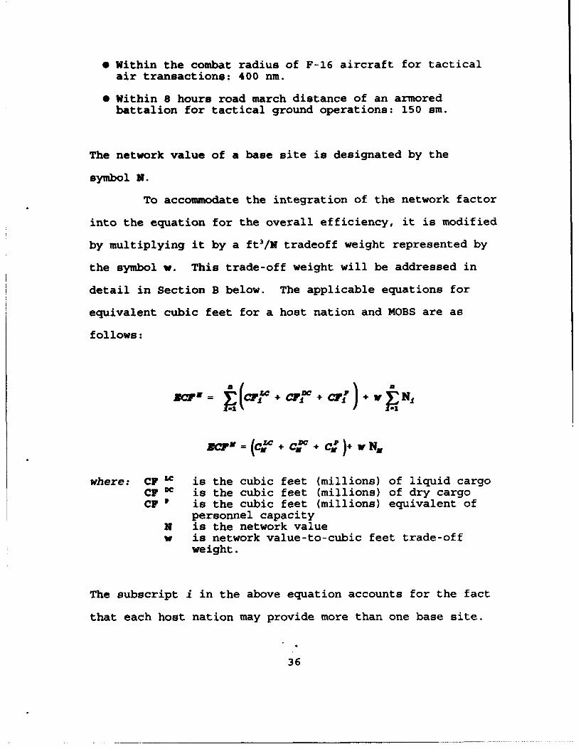
The network value of a base site is designated by the
symbol N.
To accommodate the integration of the network factor
into the equation for the overall efficiency, it is modified
by multiplying it by a ft3/N tradeoff weight represented by
the symbol v. This trade-off weight will be addressed in
detail in Section B below. The applicable equations for
equivalent cubic feet for a host nation and MOBS are as
follows:
= (ci'zr + Cw+ Ci')+vN
Jr'EN = (CZC + C + CCp)+ w N
where: CF 1 is the cubic feet (millions) of liquid cargoCF D is the cubic feet (millions) of dry cargoCF ' is the cubic feet (millions) equivalent of
personnel capacityN is the network valueV is network value-to-cubic feet trade-off
weight.
The subscript i in the above equation accounts for the fact
that each host nation may provide more than one base site.
36
Capacities are aggregated to represent the host nation as a
single node. Similarly, multiple host nations are
accommodated simply by combining Wed values for each one to
form, in effect, the regional host network as a single
entity.
3. Hostile State Offensive Capability
The offensive capability of a hostile state is
presumed to impede the efficiency of base sites, conceivably
at any of the established conflict levels. This is quite
obvious at the LRC level or above, but may be evident at
lower conflict levels as well. For example, there may exist
the potential for sabotage or terrorist actions requiring
heightened levels of security at Conflict Levels 1 and 2.
Increasing security generally impedes the flow of personnel
and material.
This element is introduced to the model as a
percentage of the raw combined cubic feet capacity. It is
represented by the symbols T' and T' as applied to MOBS and
a given host nation, respectively. The equations are:
Zj'= 17(N?'
EFF='I( rc?')
where: J = (1, 2, 3, 4, 5) for a given conflict levelT,' and T,' are on (0,1)EFFC and EFF•" are the resulting effectiveness ateach conflict level.
37
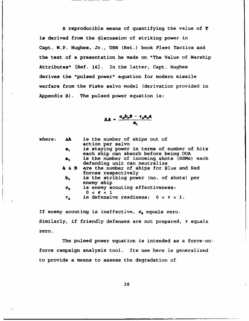
A reproducible means of quantifying the value of T
is derived from the discussion of striking power in
Capt. W.P. Hughes, Jr., USN (Ret.) book Fleet Tactics and
the text of a presentation he made on "The Value of Warship
Attributes" [Ref. 16]. In the latter, Capt. Hughes
derives the "pulsed power" equation for modern missile
warfare from the Fiske salvo model (derivation provided in
Appendix B). The pulsed power equation is:
AA = usb 2 B - TAS3A81
where: &A is the number of ships out ofaction per salvo
a, is staying power in terms of number of hitseach ship can absorb before being OOA
a3 is the number of incoming shots (SSMs) eachdefending unit can neutralize
A & B are the number of ships for Blue and Redforces respectively
b 2 is the striking power (no. of shots) perenemy ship
as is enemy scouting effectiveness:0< < I
7 is defensive readiness: 0 < 7 < 1.
If enemy scouting is ineffective, a. equals zero.
Similarly, if friendly defenses are not prepared, 7 equals
zero.
The pulsed power equation is intended as a force-on-
force campaign analysis tool. Its use here is generalized
to provide a means to assess the degradation of
38
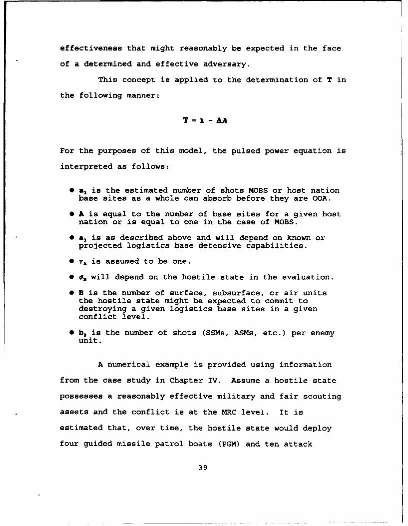
effectiveness that might reasonably be expected in the face
of a determined and effective adversary.
This concept is applied to the determination of T in
the following manner:
T=i -AA
For the purposes of this model, the pulsed power equation is
interpreted as follows:
"* a& is the estimated number of shots MOBS or host nationbase sites as a whole can absorb before they are OOA.
"* A is equal to the number of base sites for a given hostnation or is equal to one in the case of MOBS.
" a&3 is as described above and will depend on known orprojected logistics base defensive capabilities.
"* rA is assumed to be one.
"* a. will depend on the hostile state in the evaluation.
"* B is the number of surface, subsurface, or air unitsthe hostile state might be expected to commit todestroying a given logistics base sites in a givenconflict level.
"* b 2 is the number of shots (SSMs, ASMs, etc.) per enemyunit.
A numerical example is provided using information
from the case study in Chapter IV. Assume a hostile state
possesses a reasonably effective military and fair scouting
assets and the conflict is at the MRC level. It is
estimated that, over time, the hostile state would deploy
four guided missile patrol boats (PGM) and ten attack
39
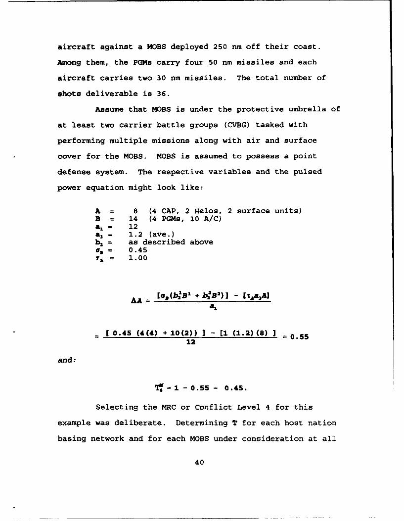
aircraft against a MOBS deployed 250 nm off their coast.
Among them, the PGMs carry four 50 nm missiles and each
aircraft carries two 30 nm missiles. The total number of
shots deliverable is 36.
Assume that MOBS is under the protective umbrella of
at least two carrier battle groups (CVBG) tasked with
performing multiple missions along with air and surface
cover for the MOBS. MOBS is assumed to possess a point
defense system. The respective variables and the pulsed
power equation might look like:
A = 8 (4 CAP, 2 Helos, 2 surface units)B = 14 (4 PGMs, 10 A/C)al = 12a 3 = 1.2 (ave.)ba = as described abovea, = 0.45
1= 1.00
AA = [a(bB + bB2)] - (,A"]
- C 0.45 (4(4) + 10(2)) ) - [1 (1.2) (8) 0.1512
and:
I= - O.55 = 0.45.
Selecting the MRC or Conflict Level 4 for this
example was deliberate. Determining T for each host nation
basing network and for each MOBS under consideration at all
40
conflict levels is unnecessarily complex for the detail
required in this model. It is suggested, therefore, that T
be determined for each of these at the MRC level only and
that it be scaled up or down for other levels accordingly.
4. The Unifying Equation
Combining cost and effectiveness into one equation
produces a decision tree with a single attribute. This
results in significant simplification of the problem and
analysis. The equation is a straight-forward determination
of equivalent cost:
zQUIVCOST =(C + CM) + V( EFF' +zFF')
where: V is in terms of COST/EFFECTIVENESS and represents atrade-off weight.
Note the occurrence here of a second trade-off weight. This
and the trade-off weight w described in subsection two will
be discussed in the following section.
B. TRADE-OFF WEIGHTS
It is useful at this point to recall that a goal of the
decision analysis is to determine the "best" alternative
among a given set of acts. In accordance with Bernoulli's
principle,
If an individual is confronted with a decision problemin which a choice is to be made from a given set of acts(risky prospects), knowing full well that the outcome of
41
a given act depends on the occurrence of a future stateof nature whose probability (of occurrence) is known orcan be estimated, the individual should then choose anact which will yield the highest expectation in terms ofthe preference over the possible consequences [Ref. 17].
Introducing the equivalent cost equation developed in
the previous section to the decision tree, and employment of
the rollback algorithm (described in most decision analysis
texts), will identify a preferred or noninferior solution.
However, if plausible variations in the values of variables
would change the preferred alternative, further analysis
must be conducted.
Ultimately, the goal is not to give the decision maker a
single solution or point estimate. Rather, it is to clarify
the interaction of variables so that the DM can better
understand the trade-offs inherent in their decision.
Trade-off weights are a means to provide this insight to the
DM and to aid in the resolution of conflicts.
1. Capacity - Network Value Trade-off (w)
The variable w does more than facilitate the
integration of units, it shows the relative value of
capacity vs. flow, which can be useful information for the
DM. For a given set of variables, plotting a graphical
solution of w against expected value will depict ranges of w
for which differing decision alternatives may be preferred.
42

2. Cost - Effe*ctiveness Trade-off (V)
Here again, a graphical solution will convey to the
DM the range for which varying levels of added equivalent
cost will indicate one decision alternative over another.
By combining an analysis of w and V with sensitivity
analysis applied to other variables within the model, a
complete and accurate picture of the decision space and
possible excursions can be provided to the DM who can then,
in turn, make an informed decision.
43

IV. CASE STUDY AND ANALYSIS
A. DECISION MODEL PROCESS FLOW
Employment of the MOBS decision model requires the
determination and tracking of multiple variables and
parameters. The flow chart in Figure 10 delineates
recommended steps to facilitate this process. The case
studies in following sections utilize this flowchart.
B. CASE STUDY BACKGROUND
Three case studies are presented. Each study represents
one of three potentially hostile states within one of the
previously identified Unified Command geographical regions.
The primary variant in each study is the Conflict Level
probability distribution. The three distributions, depicted
in Figure 11, have been chosen to represent relatively
extreme circumstances in order to exercise the model.
Parameters used in actual practice are likely to vary.
Two tools will be employed concurrently to implement the
decision model. The first is a spreadsheet model utilizing
Quatro Pro. The second is Decision Analysis by Tree Age
(DATA), which is commercial decision analysis software.
This is done to corroborate results and to illustrate that
the model can be implemented utilizing a variety of
software.
44
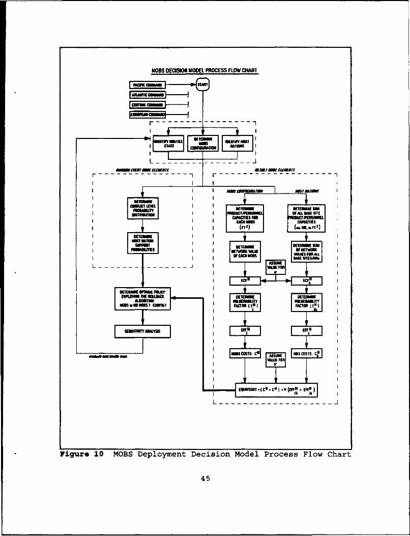
MOSS DECOM MODEL PROCESS FLOW CHART
Fmcma"M "ART
CNITIALpmFlimCimommmol
r ----- I -----------
Bpi I
I F,
I
L ---------------- J
!!I!I1ý0?ýiMOOfftWNIS XMIAW"E"Is
r --- -------- I r ------------------- 7
1
AdWaWWMnW AWJ'AMBW
calmumPROLUUTY OITý BETERNIII SUN
INOUTION PINIOUCTRENSONINI OF ALL UK Sal IC00013M FOR )PERSONNEL
UICH NOIS CAIIVMS(W) (GLNNjIFT3)
KMMKow Num
DETERMINE K sumNETWWAVAK OW:%SWUOF EACN MOOS VAMS
L - - - - - - - I - - - - - - - j
ECFn to.-'
OETEINOIý O"IK FKICvINFIrm TIRE NIUM r KWAK
MONITOR: VKNDVMTY? FAVOR (IN I FAVOR (IN I
""MuiTy
SENSITIRWANALYZ
L NOSS S: CHI NNS COM: CNIWAM Fowl
EMMOST - I CU. CU) v ;(IUEFFýW . WNk It
L ------------------- J
Figure 10 MOBS Deployment Decision Model Process Flow Chart
45

CONFUCT LEVEL PROBABILITY DISTRIBUTIONS
PROBABIUTY OF OCCURENCECL5
0a4------------------------------------------------------------------
0.2 --- -- - - ---- - - - --- --- --- ------ ----
0.2 ---- -
01 2 3 4 5
CONFLICT LEVELS
iSeries 1 1iSenries 2 ISeriens 3
Figure 11 Conflict Level Probability Distributions
The region of concern for the decision model is assumed
to have three host nations whose support would be critical
to planned contingencies .4ainst each of the hostile states.
Each host nation represents distinctly different
circumstances:
Host Nation 1. A nation whose regime is whollysupportive of the U.S. Access and use are unrestrictedin all circumstances (the probability of HNS = 1). Nopermit costs are charged for U.S. presence. Limitedresources are available.
46

Table I1 MOBS DATA
CONFIGURATION NO. COSTS CARGO CAPACITYMODULES (millions) _(ils lft)
ACQ. O&K LIQ DRY PER
STOL 3 $ 735 $ 65 2.28 3.580 0.09
NULTINISSION 6 $1325 $105 4.56 6.10 0.17
Host Nation 2. This nation provides substantialresources and a number of base sites; however, support istentative and access and use may be restricted. Permitand other costs are high.
Host Nation 3. Defined as an "emergent" host nation. Nopeacetime access or use permitted. However, this nationshares a border and has suspended formal relations withthe hostile state. Support is expected to be providedin the event hostilities escalate and the nation'ssovereignty is threatened. Several base sites would beavailable. Permit costs would be zero but there would becosts associated with establishing facilities and O&M.The proximity to the hostile state puts facilities withinthis nation at some risk.
Two MOBS configurations, derived from Brown & Root, Inc.
concepts, will be under consideration for introduction into
the region. These are identified as MOBS Configuration 1
(ST')L) and MOBS Configuration 2 (Multimission). Costs,
configuration, and capacities are delineated in Table II.
47
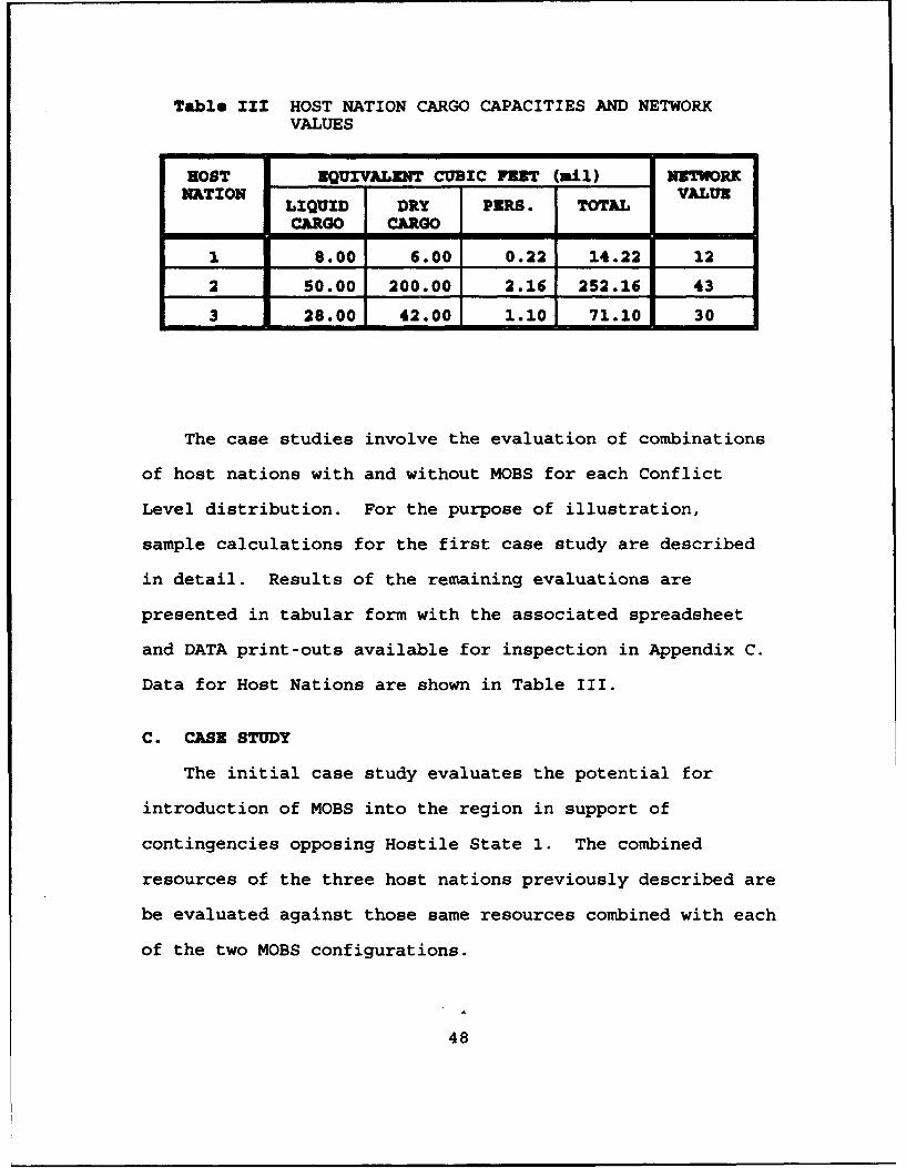
Table III HOST NATION CARGO CAPACITIES AND NETWORKVALUES
HOST EQUIVALENT CUBIC FEET (.il1) NETWORK
NATION VALUELIQUID DRY PERS. TOTALCARGO CARGO
1 8.00 6.00 0.22 14.22 12
2 50.00 200.00 2.16 252.16 43
3 28.00 42.00 1.10 71.10 30
The case studies involve the evaluation of combinations
of host nations with and without MOBS for each Conflict
Level distribution. For the purpose of illustration,
sample calculations for the first case study are described
in detail. Results of the remaining evaluations are
presented in tabular form with the associated spreadsheet
and DATA print-outs available for inspection in Appendix C.
Data for Host Nations are shown in Table III.
C. CASE STUDY
The initial case study evaluates the potential for
introduction of MOBS into the region in support of
contingencies opposing Hostile State 1. The combined
resources of the three host nations previously described are
be evaluated against those same resources combined with each
of the two MOBS configurations.
48

Table IV PROBABILITY OF HOST NATION SUPPORT BYHOST NATION AND MOBS CONFIGURATION
HOST MOBS CONFLICT LEVELNATION
CONFIG. 1 2 3 4 5I no MOBm 1.0 1.0 1.0 -.0 1.0
MOBSS1 1.0 1.0 1.0 1.0 1.0
MOBS 2 1.0 1.0 1.0 1.0 1.0
2 nO MOBS 1 0.8 0.5 0.4 0.2
MOBS 1 1 0.9 0.6 0.5 0.3
MOBS 2 1 0.9 0.6 0.5 0.3
3 NO MOBS 0.0 0.1 0.6 1.0 1.0
MOBS 1 0.0 0.2 0.7 1.0 1.0
MOBS 2 0.0 0.2 0.7 1.0 1.0
1. Random Event Node Elements
The Conflict Level probability distribution for
Hostile State 1, derived from intelligence and state
department estimates, is as shown in Figure 11. Note that
there is a high probability that hostilities will escalate.
The respective probabilities of HNS at each Conflict
Level are described in Table IV. Note that for Host Nations
2 and 3, the probability that those nations will provide
support increases with MOBS present. Recall that, in the
49

influence diagram for the model, the decision node was
assumed to influence the HNS chance node.
For the remainder of the thesis, that influence is
assumed to be that the presence of MOBS, regardless of
configuration, will increase the likelihood that HNS will be
provided.
If MOBS is being evaluated against a single host
nation, the probabilities of HNS above can be used directly
in the model. However, if several host nations are being
evaluated as a unit, the individual HNS probabilities must
be aggregated for use in the model.
Since the probability of HNS is the probability that
that nation's equivalent cubic feet are available for use,
probabilities will be weighted in proportion the individual
nation's contribution to the regional network as a whole.
For instance, from Table III, Host Nation 2 has
252.16 million cubic feet of capacity and a network value
of 43. The input value for w is 10. Host Nation 2's
equivalent cubic feet capacity is:
of oo DC +o ooNZC2= ( C"2 + C2+ CP 2 ) N2
=-(50. 00 + 200.00 + 2.16) +10(43)= 682.16.
As is shown below, the combined equivalent cubic feet
capacity of -he three host nations is 1187.48. The
50

probability of HNS for Host Nation 2 with MOBS 2 and at
Conflict Level 3 (from the table above) is 0.60.
Therefore, the weighted contribution of Host Nation 2 to the
aggregate HNS for the conditions described is:
0.6 (682.16) = 0.34.
This value is combined with that of Host Nations 1 & 3 for
the aggregate probability of HNS at Conflict Level 3 with a
MOBS 2 configuration.
Note that the calculation of the equivalent cubic
feet for the weighted HNS probability necessarily involves
the inclusion of the variable w. While it is true that
varying w will cause some variation in the weighted
probabilities, the same value for w will be used for all
calculations; furthermore, it can be shown that this
variation is relatively small and not of significant
consequence in this application.
2. Result Node Elements
The data for host nation capacities and network
values are shown in Table ITT. With this information,
combined with the MOBS data from Table II, the values for
ECF" and ECFek can be determined:
51

For MOBS 1:
zIcrMf=(C~z + C'V + c'F) + WNNK= (2.27 + 3.s5 + o.o09) + 10(7) = 75.94.
For MOBS 2:
,.C,-=( ~c. + c;" + cP) + wvN,
= (A.56 + 6.10 + 0.17 )+ 10(12) = 130.83.
For Host Nation No. 1:
Sc?1' = Tjc W + crJD + ci';) +T NV
=1(1.20+o.9o+0.06) +
(2.80+1.40+0.06) +
(4. 00+3.70o.0~9)J1 + 10 (2+3+7)
= 134.21.
Similarly, for Host Nations 2 & 3:
cFCP, = 252.16 + 10(43) = 682.16,
=7f' = 71.10 + 10 (30) = 371.10.
The value for T4' was calculated in the previous
chapter as 0.45. This value, and those for each combination
of hostile state and host nation/MOBS configuration, are
shown in Table V.
52

Table V VULNERABILITY FACTORS
VALUES FOR TAU
CONFLICT HOSTILE STATE NO.1LEVEL
uN 1 1N 2 0N 3 MOBS MOBS1 2
1 1.00 1.00 1.00 1.0 1.0
2 1.00 0.95 0.90 1.0 1.0
3 1.00 0.80 0.70 0.60 0.80
4 1.00 0.65 0.50 0.45 0.60
5 1.00 0.45 0.35 0.25 0.40
HOSTILE STATE NO. 2
1 1.00 1.00 1.00 1.00 1.00
2 1.00 1.00 1.00 1.00 1.00
3 1.00 0.92 0.90 0.95 0.98
4 1.00 0.86 0.83 0.87 0.92
5 1.00 0.80 0.75 0.82 0.89
HOSTILE STATE NO. 3
1 1.00 1.00 1.00 1.00 1.00
2 1.00 1.00 1.00 1.00 1.00
3 1.00 0.92 0.93 1.00 1.00
4 1.00 0.86 0.88 0.95 0.99
5 1.00 0.80 0.83 0.91 0.95
The Equivalent Cubic Feet value for each instance of
host nation and MOBS configuration, is multiplied by the
vulnerability factor T for each, as it has been determined
53

at every Conflict Level. The individual results for host
nations are aggregated to comprise the value for EFFz7 and
ZIFP, as determined for each MOBS. Test Case 1 examples
are:
For combined host nations:
3
NI'14j = XT~fj ( Bc4)r
= (1.00 * 134.22) +(0.65 * 682.16) +(0.50 * 71.10)
= 763.17.
For MOBS 1:
EIPF, =1 ( ZCFU)= 0.45 * 75.95= 34.18.
For MOBS 2:
EMPI,= r4 ( ZCFW)= 0.60 * 130.83= 78.50.
Finally, the product of the tradeoff variable V and
the above effectiveness values are added to the combined
host nation and MOBS configuration costs as applicable to
produce the value introduced at the decision tree result
nodes.
54
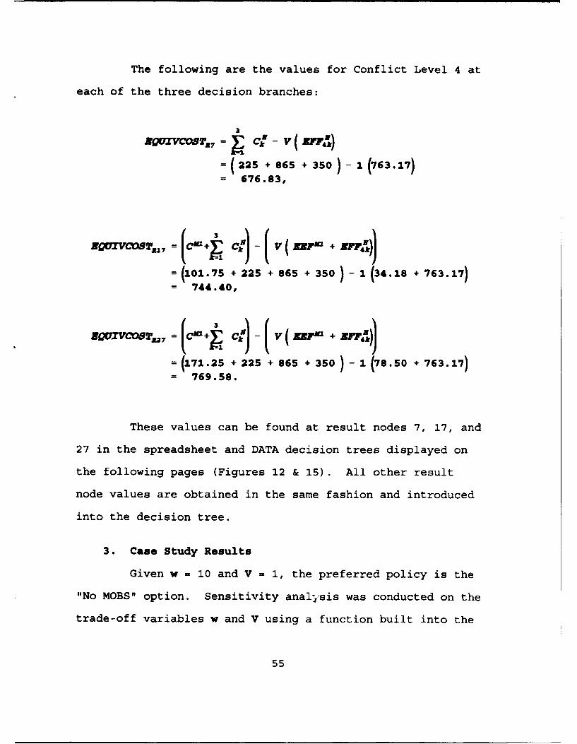
The following are the values for Conflict Level 4 at
each of the three decision branches:
u ( k - V ( "P41)(225 + 8655 + 350)-1(763.17)
- 676.83,
.oUxVCO8s.,7 = () - ( v( k))
= (101.75 + 225 + 865 + 350 1) (3,.1 + 763.17)= 744.40,
J >COS,2,7 = C j -:) V( v FMz +zr
= (171.25 + 225 + 865 + 350 )-1 (78.50 + 763.17)= 769.58.
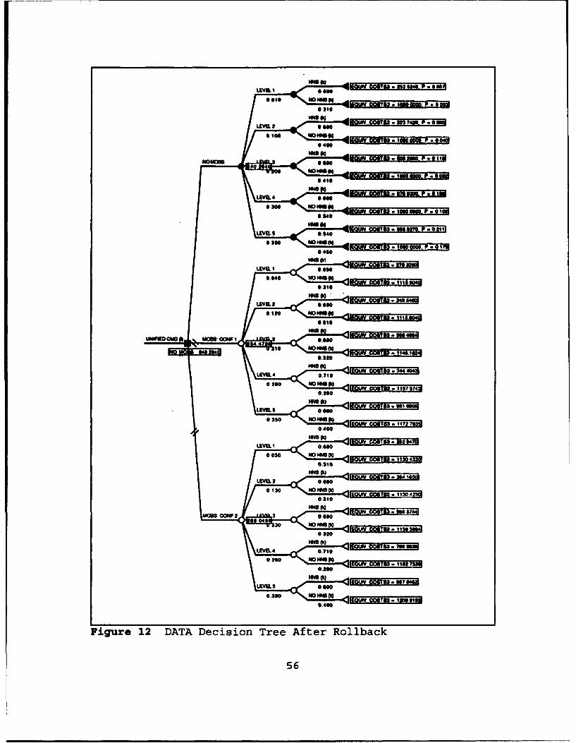
These values can be found at result nodes 7, 17, and
27 in the spreadsheet and DATA decision trees displayed on
the following pages (Figures 12 & 15). All other result
node values are obtained in the same fashion and introduced
into the decision tree.
3. Case Study Results
Given w = 10 and V = 1, the preferred policy is the
"No MOBS" option. Sensitivity analysis was conducted on the
trade-off variables w and V using a function built into the
55
MOW. eggs . 25 a .P.*0
530
S00
f4ýmm mm In
ISO mm MO .p.1
No0,u .0
- 11304
0.417
1' 1
Figure~~~~~~ma 1DAADcsoTreAtrRlbckNS
56II40.0

* C
4*e 0 0o
00N> >
z (
.J-j-
~cm
rm.1 id0I I
,0
0
• -0
0 0000 0
U) 0
-0
0
zo
O ' N '- 0 O O 0 - CO U) O
enflA peaoedx3
Figure 13 DATA Sensitivity Analysis on w
57

4* cl
0 U
0z( 00Si Oo
.J
.j.
Vz
wOU) C4
w 00
00
0 o
%.I %I %- - -
F 0
o Co
o 0 o • 0 0 0 0 00o oN C 0 0 0 0 0 0
- - C D N to I 0 CD
ent9A p8138dx3
Figure 14 DATA Sensitivity Analysis on V
58
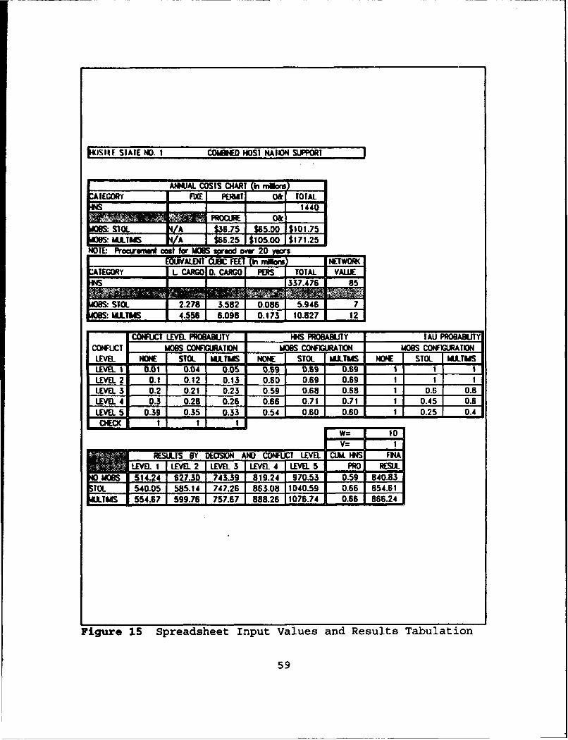
)SIR. SIAwE NO. I COMBIED HOST NAION IS•PORI
ANNUAL COSTS 04ART (inlrs•,EGOY FI1 PERMI o& TOTAL
FINS/I 1440___ 0k ___
s STOL b/A $36.75 5.00 I101.75MS kM NA I $6625 $105.00 I$171.25
NOTE- Proaamdi cost for MOBS-Swod ovr 20
IMOS STOL 2.7 .8 0.086 .5.9467
IM: UM s IUS 4.556 6.098 0.173 10.827 1 12
CONFLICT LEVEL PROBABUTY HNS PROBABITY TAU BACONFLICT MOBS CONFWIJRATION MOBS CONF1GURATION MOBS CONF1GLRATION
LEVEL NONE STOL MUIMdS NOW STOL MULTUS NONE STOL LM0LTMSLEVEL 1 0.01 0.04 0.05 0.69 0.69 0.69 1 1 1LEVEL 2 0.1 0.12 0.13 0.60 0.69 0.69 1 1 1L 3 0.2 0.21 0.23 0.59 0.68 0.68 1 0.6 0.8LEVEL 4 0.3 0.28 0.26 0.66 0.71 0.71 1 0.45 0.6LEVEL 5 0.39 0.35 0.33 0.54 0.60 0.60 1 0.25 0.4
OCECK I I IW= 10
V-- 1
RMESLTS BY DECISION AND CONFLCT LEVEL CUM, HNS FiNALEVELI LEVEL2 LEVEL3 LEVEL4 LEVEL5 PRO RESLL
MOBS 514.24 627.30 743.39 819.24 970.53 0.59 840.830T1 540.05 585.14 747.26 863.08 1040.59 0.66 854.61
TMS 554.67 599.76 757.67 888.26 1076.74 0.66 866.24
Figure 15 Spreadsheet Input Values and Results Tabulation
59
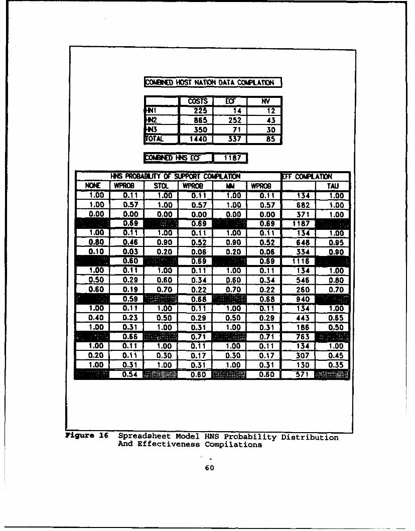
tMA H HOST tATK3H DATA COWLATKN
COSTS ECF NV____ 22.5 14 12
865 252 433S350 71 30
ro 1-1440 337 85
MCIIeM HNS ECF I =17
IiS PRO UY OF SUPPORT COMLATION COMPLATIONNONE WPROB STOL WPROB MM WPROW TAU
1.00 0.11 1.00 '011 1.00 0.11 134 1.001.00 0.57 1.00 0.57 1.00 0.57 682 1.000.00 0.00 0.00 0.00 0.00 0.00 371 1.00
0.69 0.69 0.69 11871.00 0.11 1.00 0.11 1.00 0.11 134 1.000.80 0.46 0.90 0.52 0.90 0.52 648 0.950.10 0.03 .0 0.06 0.20 0.06 334 0.90
1.00 0.11 1.00 0.11 1.00 0.11 134 1.000.0 0.29 0.60 0.34 0.60 0.34 546 0.800.0 0.19 0.70 0.22 0.70 0.22 1 260 0.70
1.0 0.11 1.0 0.11 1.0 0.11 134 1.000.40 0.23 0.50 0.29 0.50 0.29 443 0.651.00 0.31 1.00 0.31 1.0 0 0.31 186 0.50
1.00 0.11 1.00 0.11 1.00 0.11 134 1.000.20 0.11 0.30 0.17 0.30 017 307 0.45
1.0 0.31 1.0 0.31 1. 0 .031 130 0.350.54 0.60 nrQ :r7
Figure 16 Spreadsheet Model HNS Probability DistributionAnd Effectiveness Compilations
60

II
.1 44
I WI 4 p
MIDt 75tI 348
ci
613

DATA program and the resulting threshold values are shown in
Figures 13 & 14.
Note that, for this case study, only a slight
increase in v or V will result in a change to the
recommended policy for the conditions described. It is up
to the DM to decide where the threshold level lies.
D. ADDITIONAL CASK STUDIES AND ANALYSIS
A total of six iterations of the model were completed.
The first was described in the previous section. The second
and third involved the same three host nations and MOBS
configurations vs. Hostile States 2 and 3 respectively.
The remaining three runs involved assessing the impact on
policy of varying the HNS network by successive removal of a
different host nation in the Hostile State 1 scenario.
The objective in presenting the variations on the
original scenario is to provide a sample of the range of
information that analysis of the model output can provide.
1. Decision Space Comparison by Hostile State
Figures 18 and 19 depict the threshold shifts for w
and V with a change in the Hostile State (i.e. variation on
the Conflict Level distribution). Note that with Hostile
State 1, the MOBS thresholds are well to the right of
62

THRESHOLD VALUES FOR TRADEOFF VARIABLE W
CHANGES IN CONFLICT LEVEL DIST-RIBUllON
1
j2
0 4 8 12 16 20
VALUE OF W
1 No MOBS, 2=Config 1, 3=Config 2
Im aZ. 1 1-Swea. 2 mS-i.. 3V-1
Figure 18 Shift In w Threshold With Change In ConflictLevel Distribution
THRESHOLD VALUES FOR TRADEOFF VARIABLE V
CHANGES IN CONFLICT LEVEL DISTRIBUTION
1
N 2
3
0 0.5 1 1.5 2 2.5 3
VALUE OF V1 =No MOBS, 2=MOBS 1,3=MOBS2 Im. 1 D--eErSne 2 mse9i. 3 I
Figure 19 Shift In V Threshold With Change In ConflictLevel Distribution
63

those for Hostile States 2 and 3. MOBS fairs less well with
Hostile State 1, where the probability of escalation is
high, primarily because of the low vulnerability factor T.
2. Threshold Shift With Network Structure Change
Regarding w, the loss of Host Nation 3 results in a
shift of thresholds to the left, more in favor of MOBS.
With the loss of Host Nations 2 or 3, MOBS 1 is eliminated
from the decision space and MOBS 2 becomes a more attractive
alternative.
Note also that when Host Nation 3 is removed, the
threshold for MOBS 1 drops below 10, which makes MOBS 1 the
preferred policy in that instance for V fixed at 1 and w
fixed at 10. The trends for V are similar to those for w
with the exception of the situation where Host Nation I is
removed from the network. In that instance, there is slight
shift to the right. When Host Nation 2 is eliminated,
again, MOBS 1 is removed from the decision space.
64

THRESHOLD VALUES FOR TRADEOFF VARIABLE W
CHANGES IN HOST NATION SUPPORT STRUCTURE
ALL
HN 1&2
HN 1&,3
HN 2&3
0 3 6 9 12 15VALUE OF W
1 =No MOBS. 2=Config 1, 3=Conlig 2
mi...• 1 -ISane 2 mSw 3 IV-I, HOSTILE STATE NO. 1
Figure 20 Shift in w Threshold Values With Host NationSupport Structure Change
THRESHOLD VALUES FOR TRADEOFF VARIABLE V
CHANGES IN HOST NATION SUPPORT STRUCTURE
ALL
HN 1&2
HN 1&'3
HN 2&3
0 0,5 1 1.5 2 2.5 3
VALUE OF V1 =No MOBS, 2=Config 1, 3= Config 2
msemiei l-e).i.em2 mneS9n IW-10, HOSTILE STATE NO. 1
Figure 21 Shift In V Threshold Values With Host NationSupport Structure Change.
65

3. Shifts in Threshold Values With Increasing T
An increase in the MOBS vulnerability factor T
results from a decrease in MOBS vulnerability. As T
increases, it is reasonable to expect that MOBS would become
a more attractive alternative and a shift to the left would
be anticipated on the threshold diagrams. The degree of
that shift is depicted in Figures 22 and 23.
The vulnerability factor was increased first by 10%
and then 30% above the baseline value (up to 1.0). At 30%,
a change in policy is indicated by both w and V to MOBS 1 as
the preferred alternative.
This information can be useful in gauging the
marginal return for increasing MOBS defensive capabilities
or the level of protection required from other units.
4. Host Nation Support Probability
Built into the spreadsheet model is a mechanism
which returns the composite of the conditional HNS
probabilities. By noting changes in these values as host
nations are considered for deletion from the network, the
impact on the network as a whole can be gauged.
Refer to the Table VI. Note that the probability of
HNS generally declines when a host nation is deleted. For
instance, when Host Nation 3 is deleted, the probability
declines five percent for the No MOBS situation (from 59%
to 54%).
66

THRESHOLD VALUES FOR TRADEOFF VARIABLE W
DECREASING MOBS VULNERABILITY (INCREASING TAU)
BASEUNE
T + 10%
T + 30%
0 3 6 9 12 15
VALUE OF W
1= No MOBS, 2= MOBS 1, 3=MOBS 2
iSwer 1 ICSnQ 2 iSQwea 3V-1, HOGTILE STATE NO. 1
Figure 22 Shift in w Threshold With Decreasing MOBSVulnerability
THRESHOLD VALUES FOR TRADEOFF VARIABLE V
DECREASING MOBS VULNERABILITY (INCREASING TALU)
BASEUNE
T + 10%
T + 3M%
0.5 1 1.5 2 2.6 3
VALUE OF V
I1 =No MOBS, 2=MOBS 1, 3=MOBS 2
W=10, HOSTILE STATE NO. 1
Figure 23 Shift in V Threshold With Decreasing MOBSVulnerability
67

Table VI VARIATION IN HOST NATION SUPPORT PROBABILITIESWITH VARYING NETWORK STRUCTURES
HOST NATION PROBABILITY OF SUPPORTMOBSCONFIGURATION HOST NATION CONBINATIONS
_________ 1,2,3 1,2 1,3 2,3
NO MOBS 0.59 0.54 0.87 0.49
MOBS 1 0.66 0.62 0.85 0.60
MOBS 2 0.66 0.62 0.84 0.61
The exception is the instance when Host Nation 2 is
removed from the network and the host nation support
probability increases from 59% to 87% for the No MOBS
policy. This anomaly exists due to the fact that the
support Host Nation 2 provides is unreliable. Although the
probability of support increases when Host Nation 2 is
deleted, its absence results in a substantial loss in
capability.
The most significant decline, not surprisingly, is
felt with the loss of Host Nation 1, the staunch ally. The
loss of Host Nation 3 has a slightly smaller impact.
Z. SUMMARY
Provided in the previous section is a sample of the
types of analysis that the decision model affords. A wide
variety of "what if" scenarios can be generated with
68

relative ease once the basic structure is established in
either a spreadsheet model or with made-for-use decision
analysis software.
Experience with both has shown that the best alternative
is to use both spreadsheet and decision tree formats.
Spreadsheets offer the ability to rapidly alter, add, or
delete inputs. Decision analysis software, such as DATA,
provide a number of built-in tools which rapidly perform
sensitivity analysis and present the outcome in graphical
form.
69
V. CONCLUSIONS AND RECOMMENDATIONS
A. THE MODEL
Recall that the objectives in building this model were:
1. To develop an end-use perspective on MOBS.
2. To provide a pilot model for use if MOBS developmentproceeds.
3. To provide a means of assessing the efficacy ofpursuing MOBS development.
Decision analysis ia a useful tool in assessing the
importance of MOBS for effective mission support. The model
incorporates the evaluation of all of the fundamental
varia.-,es involved in an intuitive, realistic, and
reproducible format. It captures the key political and
practical interactions inherent in a decision which
necessarily involves a high degree of uncertainty and risk.
The DM is given a clear look at critical trade-offs and the
sensitivity of the value of key variables.
The model conveys the implications involved in deploying
MOBS to a specific region rather than specifics on how it
might be employed.
Finally, the model provides insight on pursuing further
development of the MOBS concept.
70

The several instances described where deployment of MOBS
in one of its configurations was the preferred policy are
perhaps less revealing than the threshold in the trade-off
values. In many instances, the range of values for the "No
MOBS" policy, though selected as the optimum, was remarkably
narrow.
This decision analysis model is intended as an aid in
the selection of MOBS deployment sites, not a complete
solution. It provides an easily implemented, supplemental
and independent tool for evaluating deployment sites from an
insightful and useful perspective.
B. APPLICABILITY OF DECISION ANALYSIS
Decision Analysis has found broad application in private
industry and government. Of the various forms of the
practice and methodology available, probability-based
decision analysis remains the most analytically rigorous and
provides results which are measurable, tractable, and
defensible.
This model has shown that complex interactions of
multiple variables can be incorporated into a relatively
simple probabilistic model which produces realistic,
practical results.
71

C. ON MOBS
The redundancy and capacity of our overseas basing
network will continue to decline by several thousand sites
in the next few years. Prepositioning, surge sealift, and
airlift offer only partial solutions. The Mobility
Requirements Study states:
The National Military Strategy... requires that theUnited States deploy a decisive force either as amember of a coalition or unilaterally and sustain it inparts of the world where adequate pre-positionedequipment or bases may not be available and where thecapability to support the force once it has arrived islimited [Ref. 181.
In the past, technology has made a decrease in
redundancy acceptable, primarily by the increasing range of
aircraft. Apart from the C-17 program, there are no such
technological advancements on the immediate horizon. The
wing-in-ground-effect aircraft holds some promise in this
regard but it is too many years away to realize its
contribution to overseas basing.
The technology necessary for the production and
deployment of MOBS is well-founded and the materials
relatively inexpensive and widely available. This, along
with a trend of increasing permit costs and the often
tentative provision of Host Nation support, combines to make
MOBS an increasingly practical and fiscally sound
alternative to land-based systems.
72

The model highlights the issue of vulnerability for
MOBS. If the basic tenets utilized in the determination and
use of Tau (the vulnerability factor) are accepted, it is
readily apparent that vulnerability is certainly a great
concern. However, in the near term, U.S. military dominance
is sufficient to mitigate the level of vulnerability against
the majority of adversaries likely within the scope a
regional conflict.
D. RECOMMENDATIONS
Increasing levels of complexity are introduced to the
basic model with relative ease. What the analyst must
realize is that the size of the model, (i.e. the number of
end nodes), proliferates rapidly. A spreadsheet quickly
becomes unmanageable as the level of complexity increases.
Even commercial decision analysis software, such as DATA,
becomes difficult to manage at these higher levels of
complexity.
In any case, the purpose of the decision analysis is to
provide insight for the DM. Unnecessarily complex models
may not be efficient or desirable in meeting this purpose.
Additional applications of the model include the
evaluation of potential land-based sites considered in the
expansion of the overseas basing network. This can be
accomplished simply by introducing the applicable data for
the prospective Host Nation in the same manner as MOBS.
73

Further, it can be used to elicit the relative implications
of the removal of existing base sites.
The model is recommended as a means to perform
supplementary analysis of MOBS deployment options. When
used in conjunction with more traditional evaluation
techniques, model outputs can be compared and contrasted.
As a result, the analyst can present the decision maker with
a more thorough perspective on the requirements for, and
implications of, their policy choice.
74

INDNOTES
1. E.I.Hickey and P. Skarlatos, Mobile Offshore Bases:Augmenting the Carrier Strike Group (Brown & Root, Inc.,[Study 10]: Washington D.C., 1991), p. 18.
2. L.B. Sohn and K. Gustafson, The Law of the Sea (WestPublishing Co.: St Paul, 1984), condensed from Chapter 7.
3. James R. Blaker et al., Global Basing (Task 3Report), The Costs of U.S. Overseas Basing (Hudson Institute[HI-3917-RR]: Alexandria, Oct. 1987), pg. 3.
4. Ibid., p. 10.
5. John F. Peel Brahtz, Modularized Ocean Basing System-A United States Option in a Strategy of DiscriminateDeterrence (Circa 2000) (Naval Civil Engineering Laboratory[R-928]: Port Hueneme, Nov. 1989), p. X.
6. Hickey, p. 31.
7. Craig W. Kirkwood, "An Overview of Methods for AppliedDecision Analysis," Interfaces, November-December 1992.,Volume 22, Number 6, p. 28.
8. Kneale T. Marshall and Robert M. Oliver, DecisionMaking and Forecasting, unpublished manuscript, June, 1993.
9. Vira Chankong and Yacov Y. Haimes, MultiobjectiveDecision Making Theory and Methodology, (Elsevier PublishingCo., Inc., New York, 1983).
10. Marshall, pp. 10-11.
11. Marshall, pp. 11-12.
12. Captain Wayne P. Hughes, Jr. USN (Ret.), Naval ForcesIn Joint Littoral Warfare, Abstract of a presentation at theMilitary Operations Research Symposium, 22 June 1993.
13. Chankong, pp. 8-13.
75
14. Military Traffic Management Command TransportationEngineering Agency, Logistics Handbook for StrategicMobility Planning, August 1989, Table 30 and Appendix E, pp.63 and 130. The conversion factor for dry cargo is theweighted average for "Mixed Dry Cargo(Less A/C)" on p. 65.
15. James R. Blaker et al., U.S. Global Basing (Task 4Report) U.S. Basing Options, Hudson Institute [HI-3916-RR),October 1987, p. 26 and Appendix C, Table 3. Blaker alsodescribes the concept of network value in his book, UnitedStates Overseas Basing, An Anatomy of the Dilemma. New York:Praeger Publishers, 1990, pp.59-82.
16. Captain Wayne P. Hughes, Jr. USN (Ret), Fleet Tacticstheory and practice. Annapolis: Naval Institute Press, 1986,pp. 254-264. "The Value of Warship Attributes". Monterey:Naval Postgraduate School, an unpublished presentation, pp.1-16, particularly p. 9.
17. Chankong, p. 90.
18. Executive summary, Mobility Requirements Study,Volume I p. ES-2.
76

BIBLIOGRAPHY
Avenhaus, Rudolph, Hassane Karkar, and Rudnianski, Michael
eds., Defense Decision Making. New York: Springer-Verlag,
1989.
Blaker, James R., et al. U.S. Global Basing (Task 3 Report), The
Cost of Overseas Basing. Alexandria: Hudson Institute (HI-
3917-RR), Oct. 1987.
Blaker, James R. United States Overseas Basing, An Anatomy of the
Dilemma. New York: Praeger, 1990.
Blaker, James R., Tsagronis, S. John, and Walter, Katerine T.
U.S. Global Basing (Task 4 Report), U.S. Basing Options.
Alexandria: Hudson Institute (HI-3916-RR), Oct. 1987.
Blaker, James R., and Wlater, Katherine T. U.S. Global Basing,
(Task 1 Report), Historical Overview of the U.S. Overseas
Basing System. Alexandria: Hudson Institute (HI-3793-RR), Aug.
1987.
Chankong, Vira and Haimes, Yacov Y., Multiobjective Decision
Making: Theory and Methodology. New York: Elsevier Science
Publishing Co., Inc., 1983.
Harkavy, Robert E. Bases Abroad, The Global Foreign Military
Presence. New York: Oxford University Press, 1989.
Hickey, E. I. and Skarlatos, Paul et al. Mobile Offshore Bases:
Augmenting the Carrier Strike Group. Washington, D.C.: Brown
and Root, Inc., Oct. 1991.
77

Hughes, Capt. Wayne P., Jr. Fleet Tactics Theory and Practice.
Annapolis: Naval Institute Press, 1986.
Hughes, Capt. Wayne P., Jr. "The Value of Warship Attributes."
Monterey: Naval Postgraduate School, an unpublished
presentation, Sep. 1993.
Kruzel, Joseph, editor. American Defense Annual, 1991-1192.
New York: Lexington Books, 1992.
Loftus, Stephen F., Vice Admiral, USN. "Supporting Forward
Deployed Forces." Washington, D.C: Naval Operational Logistics
Newsletter, Feb. 1993, pp. 1-8.
Marshall, Kneale T., and Oliver, Robert M. Decision Making and
Forecasting. Monterey: Naval Postgraduate School, 1993.
Ngantcha, Francis. The Right of Innocent Passage and the
Evolution of the International Law of the Sea. New York:
Pinter Publishers, 1990.
O'Rourke, Ronald. Naval Forward Deployments and the Size of the
Navy. Washington, D.C: Congressional Research Service, The
Library of Congress, Nov. 13, 1992.
Peel Brahtz, John F. Modularized Ocean Basing System - A United
States Option in Strategy of Discriminate Deterrence (Circa
2000). Port Hueneme: Naval Civil Engineering Laboratory
(R-928), Nov. 1989.
Sohn, Louis B., and Gustafson, Kristen. The Law of the Sea. St.
Paul: West Publishing Co., 1984.
78

APPENDIX ANETWORK VALUEI
79

BASE EVALUATIONS AND NETWORK ANALYSIS
To evaluate bases, we have adopted some of the insights and techniques ofwhat is known as network analysis. This approach, growing out of the systemsanalysis movement of the 1960s, has been developed into one of the mostuseful modes of analysis, particularly as computer assisted simulations grewin the 1970s and 19&0s. We have drawn from the work of Burt, Elmaghroby,Gordon, and Pritsker for the adaptation of the approach used in thisassessment.'
The basic assumption of our assessment is that the interactions (eitheractual or potential) between base sites form a network through which militarymanpower, materiel, and information flow. As a network, this can be modeledand network theory and measurements can be applied to identify (1) existingand potential interactions among base sites, (2) the extent to which any baseis capable of providing men, materiel, or information to any other base, and,(3) the relative value of any given base site to all other base sites, interms of providing men, materiel, and information.
Using network terminology, a base site is referred to as a node, theflows of materiel and manpower between nodes are referred to as transactions,and the connections among the nodes are referred to as branches. Nodes andtransactions have attributes that can be expressed quantitatively.
Transactions, for example, can be expressed in numbers of men, voiume, orweights of materiel, or numbers of bits of information transferred in a giventime. These transactions can be expressed in some of the measures commonlyused to analyze combat operations (eg: combat radii of a given weaponssystem) or peacetime logistics operations (eg: airlift sorties. Nodes canbe expressed in terms of capacities to receive, process, and send on men,materiel, or communications. While a wide range of measures could be used toexpress transactions and nodes, we have used the following:
- numbers of C-141 sorties transferred and processed within24 hours
- tonnages of sealift transferred and processed within 96 hours
- numbers of F-16 fighter sorties generated within 24 hours
J. M. Burt, et. al., "Simple Stochastic Networks: Some Problems andProcedures," Naval Reserve Logistics Quarterly, Vol. 17, (December 1970), pp.439-460; S. E. Elmaghroby, The Design of Production Systems (New York:Reinhold Publishing Corporation, 1966); G. Gordon, System Simulation,(Englewood Cliffs, N.J.: Prentice-Hall, Inc., 1969); A. Pritsker, Modelingand Analysis Using Q-GERT Networks (New York: John Wiley & Sons, 1977).
80

- numbers of carrier battle groups transferred and processedwithin 48 hours
- numbers of tank battalions transferred and processed within8 hours
Branches, or the connections between base sites that constitute thebasing network can be modeled in terms of rules; that is, branches among basesites can be said to exist, either actually or potentially, if it is possibleto make transactions between base sites within certain time and distanceparameters. This analysis assumed branches under the following rules:
- A branch can exist only if the sending and receiving nodes(base sites) have common characteristics (if the "transaction"involves C-141 sorties, both must have airfields capable ofsupporting C-141 aircraft; if the "transaction" involvescarrier battle groups, each must have port facilities orairfields capable of supporting carrier based combat aircraftwithin 100 miles of carrier operating areas).
- A branch can exist if the sending and receiving nodes arewithin certain distances from each other, i.e.:
- within 200 miles of the critical leg distance of theC-141; (in effect, base sites capable of receivingC-141 aircraft were considered a network if theywere within 2800 to 3200 miles of each other).
- within 3 days sailing time of Maritime Preposi-tioning Ships; (in effect, base sites capable ofreceiving sealift were considered a network if theywere within 1000 miles).
- within the combat radius (high-low-high) of F-16fighter aircraft; (in effect, all airfields capableof receiving F-16 aircraft within 575 miles wereconsidered an actual or potential network).
within 8 hours of the road march distance of anarmored column in an administrative movement; (ineffect, base sites containing fuel and bivouac spacewithin 70 miles).
- within the normal operating radius of the UH-60Ahelicopter. (in effect, all base sites within 350rmles).
The parameters selected for transactions and rules for branching werebased on operational considerations. Theoretically, of course, it ispossible for men or materiel to be transferred among any of the U.S. basesites abroad. The greater the distances between the nodes, however, the less
81

that can be transferred by air and the longer it takes to do so by anymode of transport. Network analysis can deal with these nuances, but forpractical reasons we imposed time and distance parameters that coincidewith planning assumptions used for op rations involving military systemsthat wll remain representative of the U.S. inventories over the nextdecade. The critical le$ distance of the C-141, for example, is the majortemplate used in planning airlift operations, not because C-141s are notused at lesser or greater ranges, but because this is the range at whichairlift using this system is most efficient. Likewise, the combatoperational range of the F-16 and normal operating range of the UH-60Ahelicopter, and the 8 hour transit distance of an armored column arereasonable and useful planning parameters, and, as such, have been adoptedin this assessment.
82

APPENDIX B
PULSED POWER EQUATION DERIVATION
83
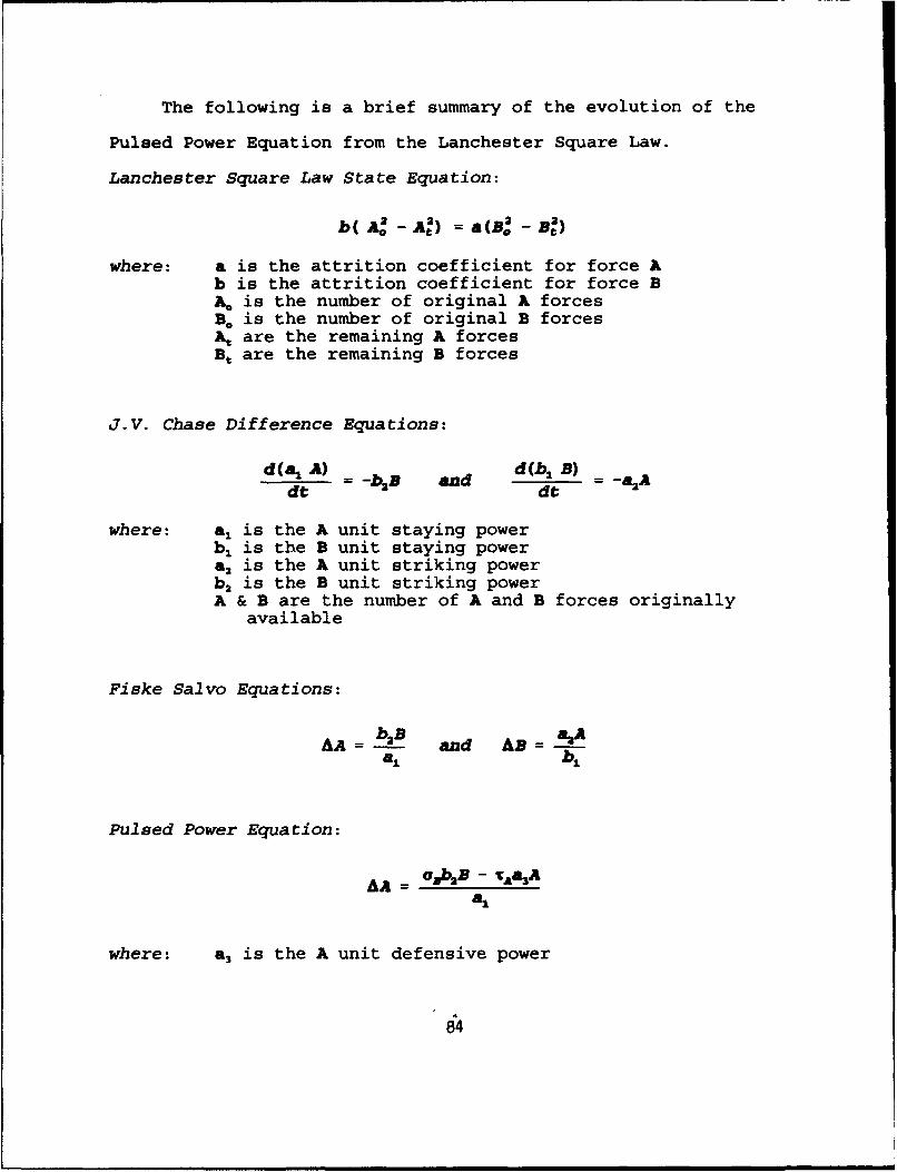
The following is a brief summary of the evolution of the
Pulsed Power Equation from the Lanchester Square Law.
Lanchester Square Law State Equation:
b( A: - A) = a(B t - B)
where: a is the attrition coefficient for force Ab is the attrition coefficient for force BA is the number of original A forcesB. is the number of original B forcesAk are the remaining A forcesBt are the remaining B forces
J.V. Chase Difference Equations:
d(al A) _ -b 2B and d(b 1 B) _ _a2 Adt dt
where: a, is the A unit staying powerb, is the B unit staying powera2 is the A unit striking powerb2 is the B unit striking powerA & B are the number of A and B forces originally
available
Fiske Salvo Equations:
A- b 2B and A =- 'Aa-- b,
Pulsed Power Equation:
AAr= E baB -ve oea,
where: a3 is the A unit defensive power
84

APPENDIX CMOBS DEPLOYMENT MODEL TEST CASE RESULTS
SPREADSHEET AND TREE AGE MODELS
85

HNS ~ ~ ~ (1 IEUVCU N51 OSTILE ifTATE 9LEVEL~~I IC OOMHST NA7MO SUPPOR
0.200 NOHWOOI _________________ LL3 HW NTK
0.310T.34
HNS IQ EOUIV-00678 - 10290A
0.2 0 N H S (0 lioiECU M - logo-.0.4600
HN k ECUIV 00678 . 2.326 -01
00 N N 1 EOUIV coSMS . 1115.600P- .6
HN 1 eOUIV COSM~ . 411.13.6401 .6
EQUIY4 00.3 673661P* .
0.00 N HS(k EOUIV COSTS3 - 111.00 3P-0.6
0.190 NOHN(IQ0.P .0
LEVELS0.5400
0.230 NO HNS (10 IEOUIV 006783 - 110.4000
HNS (k) EOUIV COST8 - 2923)4 -0.5
0.220 NOHS(1c IEQUIY COSTS3 - 111.0.40P ýi
MS (k) IeQUIV COSTS3 - 2678.32 .P-015
0.210 NO HNS (10 EOUIV 006783 - 1133. aP - .05
HNS k) EOUIV CT83.a 462908.0026 Oj
010 NHNS (k) ECIFYI 00653 . 114.70.6W -0.
LEVU4 008183. 536.54
0.190 N=!LNS " <EQUI COST83 - 1144.61 P- -i
0.400
HN () JE UV OTS 862940

HOSTILE STATE NO. 2, ALL HN: V
$200 A MOBS: CONF2
$100 * MOBS: CONF 1$0- * NO MOBS
a ($1000) Threshold Values:S($2000)- •W - 1.193
> EV $456
S($3000)- W 0.879*" ••EV =$712
u ($4000)-
x ($5000
($6000)-
($7000)-
($8000)-0.000 2.000 4.000 6.000 8.000 10.000 UNIFIED CMD ()
87

HOSTILE STATE NO.2, ALL HN: W
$1300 A MOBS: CONF 2
0 MOBS: CONF 1$1100 * NO MM
$900- Threshold Values:
•. W -8.523$700 EV - $702
"CDo W - 12.146
S$500- EV- $485
0.
,,, $300-
$100-
($100)-0.000 4.000 8.000 12.000 16.000 20.000 UNIFIED CMD )
88
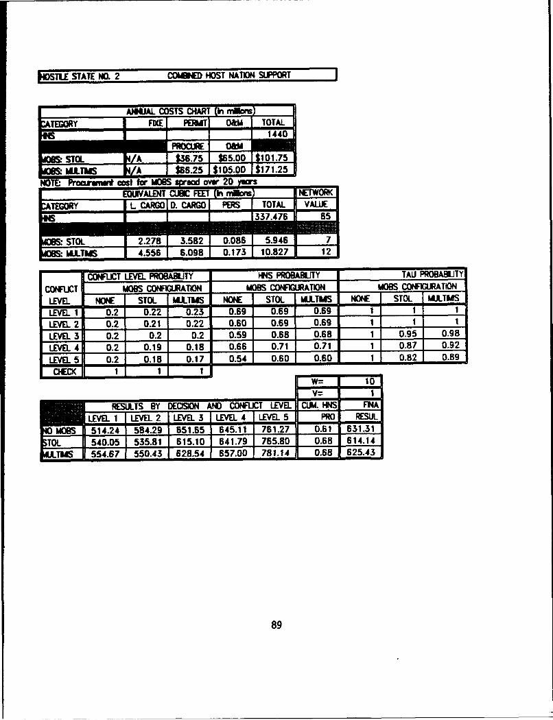
WSTLE STATE NO. 2 COMEED HOST NATION SUPPORT
LE/ NONE STOUL COSTS NST (NONiID( TERIY O& TOTAL.
LE L 02 A 02 6.75 02 5.00 $0 06 1.11gALEVE 2 /A 021 0225 .1 0 50 0 9 1171.25 1
NOTF- SWro'arwrw cost for MdOBS mrooW over 20 yewos,/ •EOIVLENT CUBC FEET (inM •) NewRI
ctEGoRY IL CARGOI D. CARGOl P I TOTAL I Au
LEVEL 32.2 7 0 3.52 1 0.0615.94068 0.5 17.5 09
M ULEVEL 44.2 5 0.19 80 18 0.663 [0.871 0.121 087 09
CONFL.ICT LEVEL PROBABILITY HNS PRBAUY TAU PROABtITY
CONLJT MOB COW lURTION MOBS .CONRFUTION MOBS CONFIGURTION
LEVEL NONE STOL WXJLTMIS NONE STOL MUATliS NONE STOL MU.LTIMSLVL1 0.2 0.22 "0.2r 0.69 D.69 0.69 1 1 1
LEVEL 2 0.2 0.21 0.22 0.60 0.69 0.69 1 1 1
LEVEL 3 0.2 0.2 0.2 0.59 0.68 0.68 1 0.95 0.90
LEVEL 4 0.2 0.19 0.18 0.66 0.71 0.71 1 0.87 0.92
LEVEL 5 0.2 0.18 0.17 0.54 0.60 0.60 1 0.82 0.89
C9ECK 1 1 1
W-- 10S- iV=
RESULTS BY DECISION AND CONFLICT LEVEL CLOW. INS FINA
LEVEL 1 LEVEL 2 LEVEL 3 1LEVEL 4 LEVEL 5 PRO RESUIL514.24 584.29 651.65 645.11 761.27 0.61 631.31
Tr 540.05 535.81 615.10 641.79 765.80 0.68 614.14
. 554.67 550.43 628.54 657.00 781.14 0.68 625.43
89

tOM HOST NATION DATA COMPLATION
COSTS ECF NVJ1 22 14 12
865 252 43- 350 71 .30
OTAL 1440 337 85
ENL IHNSECr r 1187
______ #1 PROBABLITY OF SUPPORT COMPILATION ____ COMPLATIONNONE WPROB STOL WPROB MM WPROB TAU
1.00 0.11 1.00 0.11 1.00 0.11 134 1.001.00 0.57 1.00 0.57 1.00 0.57 682 1.0000.00 0.00 0.00 0.00 0.00 371 1.00
0.69 0.69 0.69 1171.00 0.11 1.00 0.11 1.00 0.11 134 1.00
0.0 0.46 0.90 0.52 0.90 0.521 682 1.000.0 0.03 0.20 0.06 .20 0.06 371 1.00
0.60 0.69 0.69 11871.00 0.11 1.00 0.11 1.00 0.11 1314 1.000.50 0.29 0.60 0.34 0.60 0.34 628 0.920.60 0.19 0.70 0.22 07.0 0.22 334 0.90
0.59 0.68 0.78 10961.00 0.11 1.00 0.11 1.00 0.11 134 1.00
0.0 0.23 0.50 0.29 0.50 0.29 587 0.861.0 0.31 1.00 0.31 1.00 0.31 308 0.83
1.0 0.11 1.00 0.11 1.00 0.11 134 1.000.20 0.11 0.30 0.17 0.30 0.17 546 0.801.00 0.31 1.00 0.31 1.00 0.31 278 0.75
0 .54 0.o0 0.60 9580
.90

LVL10.61 253 1440 1117 1740.2 r3 2 514
0.11030 1030 0 341- - - - -
LIL 0.60 253 1440 1117 1520.2 ~ 4 534
0.40 1-0390 1030 0 432
LEE -9344 1 446. 1096 2M0.2 r - P.- 52 631
0.41 1030 logo 0 443g7
LEVE 0.6 411V I40 1029 213 -
R0.344 1030 1030 0 376
LEVEL 0.54 1432 11440 3583 2601 0.2 IS106 1r1 6
L0.46 11030 11030 0 501
LEVEL 0.6 273 1542 1263 1___10.22 r 2 4060.31 1116 1132 76 343
LEVEL 0.6 273 1542 1263 1930.21 r11463
WeLEVEL 10.61 374 1542 1163 253CaMDt 0.2 Nor1646 1
0.32 1120 1132 72 362
r 3LEVEL. 0.71 447 1542 1035 3130.13 HE146 4
0.23 1126 1132 66 323
LEVEL 10.60 521 1542 1021 3120.13 166er 0 6
LEE .9233 1611 1224 202
0.32 1133 1261 1231 367
11410.99 12611 1208 203_
0.40 1145 1261 1316 3460
r 95

LEE I NS IE CS"- MR OHOME XTATE 30.390 No HNB (10COWIIED HST NATION SUFO
0.10 IEUI CIF .-10.00 AL.L 3 HOW ATIOI
HNS~~i M oEO COSTS3 - 210.
0..300
""ý.ý0 IOIV CWMS 7.35 020.430 ~NOHS (N 404 ..
760" 0OTS.596 P-0.20.320NO NNOG @0 I IV 009M -1l11.030 PO
LEVELAI CUDo IE(I MOIS: CON 1
6. 660.340
HN (Q EOUIV COSTS3 -422.187 -
0.10N 40N (0 IEOUIV COMBS3-1 636i .00
0.460ST3 13.
HNS (k) EQI -COSTS3 - 292.94 P 029
0.340 ~ ~ ~ .3 EOI OTS.13.
HNS IEQ~UIY C09MS : 79321&P-.3-1
LOIJIY 0.690-110.
0. 0 NO HNS (10 EOUIV COST83 -4134.000 P-6-W
0.4100
0,22

HOSTILE STATE NO. 3, ALL HN:V
$2000 A MOBS: CONF 2
$1000 * MOBS: CONF 1
$o- 0 NO MOBS
CD ($1000)- Threshold Values:
" ($2000)- V -1.2> EV - $381- ($3000)iC e*V - 0.86
(40 0), *AEV - $676C.0 ($4000)
La ($5000)-
($6000)-
($7000)
($8000)-0.000 2.000 4.000 6.000 8.000 10.000 UNIFIED CMDQ)
93
HOSTILE STATE NO. 3, ALL HN: W
$1400 A MOBS: CONF 2
$1200 * MOBS: CONF 10 NO MOBS
$1000-o) Threshold Values:
$800- *A W - 8.353> EV - $662V $600-
$600- W - 12.217
EV - $414x $400-x
"La. $200-
$0-
($200)-0.000 4.000 8.000 12.000 16.000 20.000 UNIFIED CMD(I)
94
ISLE STATE NO. 3 COMBfID HOST NATION SUPPORT
ANNUAL COSTS CHART (in rrmorTEOYFIXE| PERMIT O&M TOTAL.
1440PROCURE O&U
__:_STOL N/A S36.75 $65.00 $101.75SMuLTU s E A 1 $6 .25 $105.00 $171.25
NOTE Procuromin cost for MORS spread over 20 yarsIEOUIVALENT CUBIC FEET (in nmons) NETrWORK
.,ATEGORY L CARGO I D. CARGO PE]S TOTAL VALUE1IS337.476 1 85
OS:STOL 2.278 3.582 0.086 5.946 7O M.A.TIMS 4.556 6.098 0.173E10.827 12
CONFLICT LEVEL PROBABILJTY HINS PROBABILITY TAU PROBABILITY
CONFLICT MOBS CONF•(URATION MOBS CONFIGURATION MOBS CONFIGURATIONLEVEL NONE STOL MUL TMS NONE STOL MULTIMS NONE STOL MULTIMIS
L - m9 03 05 - - -LEVEL 1 0.39 0.43 0.45 0.69 0.69 0.69 1 1 1LEVEL 2 0.3 0.32 0.34 0.60 0.69 0.69 1 1 1
LEVEL 3 0.2 0.19 0.17 0.59 0.68 0.68 1 1 1LEVEL 4 0.1 0.05 0.03 0.66 0.71 0.71 1 0.95 0.99
LEVEL5 0.01 0.01 0.01 0.54 0.60 0.60 1 0.91 0.95CHECK 1 1 1
W= 10V= I
RESULTS BY DECISION AND CONFLICT LEVEL CUM. HNS FINALEVEL 1 LEVEL 2 LEVEL 3 LEVEL 4 LEVEL 5 PRO RESUL
M 514.24 58429 64511 63295 745.23 0.64 57561T 540.05 535.81 603.77 622.49 741.22 0.69 556.94
TIMIS 554.67 550.43 618.39 634.62 1 755.54 0.69 568.47
95

KOMWD HOST NATION DATA COMWLATION
COSTS EC" N1 225 14 122 865 252 43
•I3 350 71 .30
OTAL 1440 337 85
ICHWM NSECFI 1187
_____HNS PROBABUITY OF SUPPORT COMPLATION ____F COMPLATIONNONE WPROB STOI. WPROB mm WPROB TAU
1.00 0.11 1.00 0.11 1.00 0.11 134 1.001.00 0.57 1.00 0.57 1.00 0.57 682 1.000.00 0.00 0.00 0.00 0.00 0.00 371 1.000. 6.. 9 0.6..._L9 0.69...L 1197,1.00 0.11 1.00 0.11 1.00 0.11 134 1000.80 0.46 0.90 0.52 0.90 0.52 682 100.10 0.03 0.20 0.06 0.20 0.06 371 1.00
S0.60 0.69 0.69 1187
1.00 0.11 1.00 0.11 1.00 0.11 134 1i.O0.50 0.29 0.60 0.34 0.60 0.34 628 0.920.60 0.19 0.70 0.22 0.70 0.22 345 0.93S~0.5-9 0.68 0.68 1107 JJl•
1.00 0.11 1.00 0.11 1.00 0.11 134 1.000.40 0.23 0.50 0.29 0.50 0.29 587 0.861.00 0.31 1.00 0.31 1.00 0.31 327 0.88
0.66 0.71 0.71 10471.00 0.11 1.00 0.11 1.00 0.11 134 1.000.20 0.11 0.30 0.17 0.30 0.17 546 0.801.00 0.31 1.00 0.31 1.00 0.31 308 0.83
,"0.54 0.60 MI= 0.60 [ 988
96

L~rriLEVEL 0.*63 2m 1440 1157 174 - -
0.39 *a - 2 5140.31 1030 1030 0 341 - -
r.3LEVE 0.50 253 1440 1157 152 -
0.3 1 - 5540.40 10.0 1090 0 -
O.OS
LEVEL. 0.59 33 1440 1107 16 -
0.2 W6 6 645 5760.41 1000 1030 0 449
r 7LEVEL 0.56 393 1440 1047 257 - -
0.1 r3 8i 6330.344 1090 1090 0 3756
LEVEL 0.54 452 1440 955 244
R00.3
0.01 r160.45L 1030 1090 0 501
LEVEL. 0.63152 123 90.43 16r 12 540 ___
0.1 1115 1132 76 341 ___
LEVEU 0.9 275 1542 1263 1933 _ __
0.32 13 14__ 5360.3 116 1192 75 343 ___
r 15 ___
BlUE LEVEL 1 0.65 5 52 16 4
2~i M36 ,- 192 __35
r 17 ___
LEVEL 0.1 422 1542 1120 3010.05 16r 18 622
0.9 1120 1192 72 322 - -
r. 19LEVEL 1 0.60 455 1542 1057 290 - -
0.01 136 r 20 74
0.40 1123 1132 69 451
LEVEL 0.9293 1511 1319 2010.45 13555_ ___
0.1 1130 1261 131 353r 23 ___ __ _
LEVEL 0.6 293 1611 1315 203 ___
0.34 r3 24__ 5500.11130 1261 131 348 ___
r 25LEVEL 1 0.68 373 1511 1239 253 - -
0.17 136HN r 26 616 5680.2 1130 1261 131 3566
LEVEL 0.1 434 __ 1611 _ 1177 31
0.03 16 - r 29B___ 635 -
- .9 -1132 1261 130 325 -
LEVEL 0.60 493 1611 1112 2961 0.01 16 r__30_ 756
0.40 1137 1251 124 457 - -
97

LEVE 1 0..O HOSTILE WATE i0COIED~ HOST NATION SUPPORr
0.010 NOHGM IOI OT3- [4,00,pn OW NATIONS 2 3SONLY
LEVE 0.50 iow olm- =2M. P 0.El
ýM (k) WIV com .0d0. P. 0.1iN M09.1 00 0.640 I -sooop-t
00 DHMlo EOUIV 006T8 - 778.1*30 P - 0.16f
0.4620
0.040 NO HNS (1 !i) Uo 006183 P* sa.
0.3908. 90
HNS k) EOUIV 8OT3.9217.12430 .8
LEVELV 000T8 .653
0.280-C ýNO I 4MB IEQWV COSTS3 -93257&
LEVEL 108 0.66.006111,11,1 NOHNS k) EOUIV 00 18S3:-N6776o
0.350
HNS () 41EOUIV C06T83 -0025-.71M
* NOHNS IQ EOUIV C06183 -273.38
HNS k) flOUIV C06T83 - 00.
LINIFRIED~~OUI 006183-ON I I A0.4 476.0"0
io No"Moo llloWV 06T83.-921.Sse4
LEVEL 00883.676
0.260 NO IS (k 1EOUIV 006183 - 957.
LEVELS 0088 50.0
0. 0 O HN (IQ IEOUV 006183-963 .70190.450
HNS (k8

HOSTILE STATE NO.1, ALL HN-HNI:V
$1500 A MOBS: CONF 2
$900 * MOBS: COW 1
*NO MOBS$300-
' ($300) Threshold Values:V - 1.215
> ($900)- EV - $633
"O ($1500)V V- 1192
- ($2100)-
($2700)-
($3300)
($3900)-0.000 2.000 4.000 6.000 8.000 10.000 UNIFIED CMD()
99

HOSTILE STATE NO. 1, ALL HN-HNI: W
$1180A MOBS: CONF 2
$1090 MOBS: CONF 1$ NO MOBS
ID $910, Threshold Values:
TEST1 COST - 12.41S $820- EV - $65 1
C)CL $640-x
$550-
$460-
$370- ••
0.000 4.000 8.000 12.000 16.000 20.000 UNIFIED CMD (I)
100

140STLE STATE NO. 1 COWMM, HOST NATIONS W OUT HN1I
_Ns _ 1 1215SSTOL b/A 1 136.7s5 1$6.00 1$101.75
* MLIS /A5 1$6.25 $105.00 $171.25NOTE: Promrwmwt cost for MOBS spread ovr 20EQUVALENT CUBIC FEET (in remor) IINeTWOrKI~i
SY L CARGOI D. CARGO I PESI TOTA.L 0VALUE
WiOB:STOL 22835200615H4
NOBS:, MULTMIS 4.556 6.098 0.173 10.827 12
CONFLICT LEVEL PROBABITY HNS PROBABIJTY TAU PROBABLJTYCONFLICT MOBS CONFIGURATION MOBS CONFIGURATION MOBS CONFIGURATION
LEVEL NONe StL IMULtMs NON STOL MULTUS NONE STOt. )AJTISLEVEL 1 0.01 0.04 0.05 0.65 0.65 0.65 1 1 1LEVEL 2 0.1 0.12 0.13 0.55 0.65 0.65 1 1 1LEVEL 3 0.2 0.21 0.23 0.54 0.54 0.54 1 0.6 0.8LEVEL 4 0.3 0.28 0.26 0.61 0.58 0.68 1 0.45 0.6LEVEL 5 0.39 0.35 0.33 0.48 0.55 0.55 1 0.25 0.4
CHEK 1 1 1W= 10Y= 1
RESULTS BY DECISION AND CONFLICT LEVEL CU_. HINS FINALEVELL 1LEVEL 2 LEVEL 3 LEVEL 4 LEVEL 5 PRO RESUL
IuO MS 409.52 515.25 621.20 694.45 823.15 0.54 709.22435.33 477.85 631.83 743.95 900.28 0.62 730.85
TUS 449.95 492.47 642.24 769.13 936.44 0.62 743.23
101
tO&MED HOST NATION DATA a•fLATION
[COSTS ECF NV10 0 0
1N 865 252 4383 350 71 30
rOTAL 1215 323 73
VjOff)HNSECF 10531
__ S PROBABIITY OF SUPPORT COMPtLATION ___ COMPILATIONNONE WPROB STOL WPROB mm WPROB TAU0.00 0.00 0.00 0.00 0.00 0.00 0 0.001.00 0.65 1.00 0.65 1 .00 0.65 682 1.000.00 0.00 0.00 0.00 0.00 0.00 371 1.00
0.65 0.65 0.65 1053 M0.00 0.00 0.00 0.00 0.00 0 0.000.80 0.52 0.90 0.58 0.90 0.58 648 0.950.10 0.04 0.20 0.07 0.07 334 0.90
0.55 0.65 0.65 9820.00 0.00 0.00 0.00 0.00 0 0.000.50 0.32 0.60 0.39 0.60 0.39 546 0.800.60 0.21 0.70 0.25 0 70 0.25 260 0.70
0.54 0.64 0.64 8050.00 0.0 0.0.0 0 .00 0.00 0 0.000.40 0.26 0.50 0.32 0.50 0.32 443 0.651.00 0.35 1.00 0.35 1.00 0.35 186 0.50
0.61 0.68 0.68 6290.00.00 0.00 0.00 0.00 0.00 0 0.000.20 0.13 0.30 0.19 0.30 0.19 307 0.451.00 0.35 1.00 0.35 1.00 0.35 130 0.35
0.48 0.550
102
-w By -S .112.. 1215 !053 105
.1 r410o.3 oSS 355 0 305
LEVEL -2- - 2 -129
r 50.1 ,r4s I510 o I5o
.40 165 355 0 3265
r 7
.545
0. 2 121mo 0 2 621 709.4865 365 0 402
0.1536 1215. 629 358 -
3 r 6 634B6S 865 0 336
~LAEUL *7 1215: 43 7. r - ;,L ,-,I,-I ,I -I I
0.33 136 10 823IF- - 6 [865L4 0Z 448 ~
r ilLEE 0.6l 1317 1123 1210.04 r 12 435
035 1 67 76 314r 13
L[I. 0.5253 1317 1053 163O0.12 13 r14 47 -
0.35 3 67 76 1 30 -
r r15Ulmw dO I 0 .34 466 II 1317. 551 2 96 lICUoot 0.2 - --- 632 731
096 21 3 67 46 336r 17
L. 0.63 l654 1317 663 4420231 r6 744
0.32 333 367 34 302 -
r 13LEVL. •10.55 1 361 1317 456 4710.35 06 r 2066
0.45 343 367 13 430
LEM 0.65 202 1336 1134 1310.05 16 r 2
0.35 305 1036 131 313r 23
LEVEL 0.65 273 1336 1113 1730.13 136 r2442
0.35 305 1036 131 314r25
I ILEVEL 0.64 476 1336 310 3020.23 16r 2664 73
0.36 332 1036 105 340r27
-E-- 0.68 673 1336 707 4530.26 136 r- i 769
353 1036 73 310
LEVEL I0.55 337 1336 4U3 4300.33 N136 r 30 936
0.45 3384 1036 .2 446103
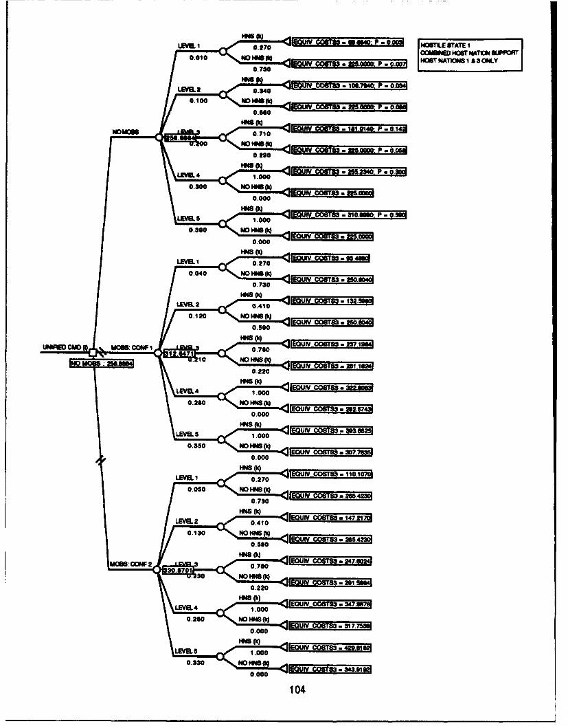
LEVEL~~ ~~ ~ ~ 1 .7 M oo-an OSTILE STATE IOdkWD MOST MATON SftPVOMT
0.01 NOMOO OW=- 25,00, p- 0 HOWTNATION1 3SONLY
HN P.00
LEVELI0.340 EQUIY- COSYSS - la¶.uso- P .-0.03
0.600
0.040o O tS(k) _________._514
.710
moz m -,QEOIJIY COSTS - 280371 .p
LEEL 83.000.
0. ~ ~ ~ ~ 3 NO.571 S M ,n
0.000
HNS (k)W 1 ýCOSTS3.FO M.0.10
0.30 NMM~o EOUIV COSTS - 14721
0.000
H.N- I104 -

HOSTILE STATE NO. 1, ALL HN-HN2:V
0 A MOBS: CONF2
$200 * MOBS: CONF 1
* NOMOBS($600)-
* Threshold Values:($1200)- AW - 1.861
>. EV - $22
0 ($1900)-
U0 ($2600)-xLJ ($3300)-
'
($4000)-
($4700)-T0.000 3.000 6.000 9.000 12.000 15.000 UNIFIED CMD()
105

HOSTILE STATE NO.1, ALL HN-2:W
$70 A MOBS: CONF 2
$60 * MOBS: CONF 1
$500 6 NOMOSS
CD $400. Threshold Values:$30 W - 19.443
EV -$40
$200-S
$100-0.x $0-
($100)-
($200)-
($300).- -0.000 6.000 12.000 18.000 24.000 30.000 UNIFIED CMD )
106

WTsE STATE NO. 1 COBINED HOST NATIONS W/OUT HN2
___________ANNUAL COSTS COHART (~rainItEGORY FIX ! PEFA1 0&1 TOTAL_____ _ __ ____ 575
____s._toL _ L $36.75 $65.00 $101 75Wm, MULTMS UA $66.25 1$105.00 $171.25NOTE: Procuremmt cst for MOBSse ov 20 ywm
EQUIVALENT CUBIC FEE ti reMora MeTWOrKKtTGR !L CRO D.CRO PR TOTAL VALUE
- STOL 2.278 3.582 0.086 5.946
NO3BS, MLLTWS 4.556 6.098 I0.173 10.827 12
CONFLICT LEVEL. PROBABILTY HNS PROBABILTY TAU PROBABILITYCONFLICT MOBS CONFIGURATION MOBS CONFIGURATION MOBS CONFIGURATION
LEVEL NONE STOL MULTMS NONE STOL MULTMS NONE STOL MULTIMISLEVEL 1 0.01 0.04 0.05 0.27 0.27 0.27 1 1 1LEVEL 2 0.1 0.12 0.13 0.34 0.41 0.41 1 1 1LEVEL 3 0.2 0.21 0.23 0.71 0.78 0.78 1 0.6 0.8LEVEL 4 0.3 0.28 0.26 1.00 1.00 1.00 1 0.45 0.6LEVEL 5 0.39 0.35 0.33 1.00 100 1.00 1 0.25 0.4COW1 1 I
W= 10V= 1
RESULTS BY DECISION AND CONFLICT LEVEL CUM. IHS FINALEVEL 1 LEVEL 2 LEVEL 3 LEVEl 4 LEVEL 5 PRO RESLI
8MOBS 13.75 184.92 193.94 255.23 310.90 0.87 256.94TOTI 209.55 202.05 245.89 322.81 393.66 0.85 312.64
TMIS 224.17 216.66 j 257.29 347.99 429.82 0.84 330.87
107

•INO HOST NATION DATA COMLATION
COSTS ECF NV_1 225 14 12
_0 0 0350 71 30
OT 575 85 42
rOMM EcF =5ss
_ HNS PROBABILfTY OF SUPPORT COPLATION _ F COMPLATIONNONE WPROB STOL WPROB MM WPROB - TAU
1.00 0.27 1.00 0.27 1.00 0.27 134 1.000.00 0.00 0.00 0.00 0.00 0.00 0 0.000.00 0.00 0.0 .0 0.00 0 0.00 371 1.00
0..27 0.27 0.27 5.00 0.27 1.00 0.27 1 00 0.27 134 1.00
0.00 0.00 0.00 0.00 0.00 0.00 0 0.O00.07 0.20 0.15 0.20 0.15 334 0.900.34 0.41 0.41 4
1.00 0.27 1.00 0.27 1.00 0.27 134 1.000.00 0.00 0.00 0.00 0.00 0.00 0 0.00
.0 0.44 0.70 0.51 0.70 0.51 260 0 700.71 0.78 0.78 394
1.00 1.00 0.27 1.00 0.27 134 1.000.00 0.00 0.00 0.00 0.00 0.00 0 0.001.00 0.73 1.00 0.73 1.00 0.73 186 0.50
1.00 1.00 1.00 3200 0.27 1.00 10.27 1.00 0.27 134 1.00
0.0 0.00 0.00 0.00 0.00 0.00 0___ 0.00__
1.00 0.73 1.-00 0.73 1.00 0.73 130 0.35
-108
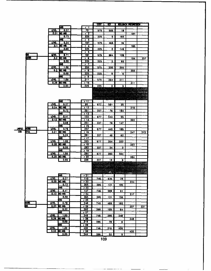
LI'ILEVL 0.27. 70 575 505 Is -
0.01 be6 r2 140.73 225 22S 0 165
r.3LEVEL 0.34 107 575 45 36
0.1 6 4 1850.5 225 225 0 14t
L5ww IIII S57 344 126-
0.2 106 - - - 134 2570.3225 225 0 6.6 -
r'7LE 100EL 255 57 320 25-5
0.3 16 - ri - 2550.00 225 225 0 0a
1LEVEL 1 .10031 57 26 310.33 116
0.00 1 1225 1 225 1 0 0
0.04 r160.73 251 327 76 104
0.120.53 251 327 76 147
WIED LEVEL 0.73 237 677 440 1Mcm1OR __0.21 106i r 16_ 247 313
0.22 211 327 46 62
L.EVEL 1.0032 67 35 330.23 K06 323
0.00 233 327 34 0
LrII
LEVEL 1.00 334 677 233 3340.35 3r6
0.00 303 327 19 0
LEVEL. 0.27 110 74_63 _2
0.05 106r 20.73 265 396 131 135
r 23LEVEL 0.41 17 76 59 6
0.13 It6 2170539 265 336 131 156
r 25LEVEL 0.7 248 746 1 433 19330.23 166 r 2625 31
0.22 22 36 15 6r~ 27
LEVEL 1.00 348 746 333 3480.26 W06 1 348
0 3 336 78 0Fr 23
LEVEL 1 1.00 40 7496 1 316 4300.33 IS06 r 30 1 1 430
0.009
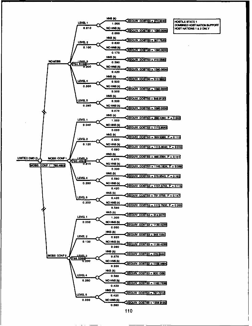
HNS k) EQUN-WY r$ 8 3. H OSTILE STATE 1LEVEL 1.00 COMMED HOWT NA11U4 SUPPORT
0.010~u NOHS(QO--UVCW HOST NATON8 I A 2 ONLY
0.10 NHN5~ ____0.0____0
0.100 NO HNS (10 leu CoeST3 . 1090.00
0.170
94.I1 0078.Q29420P 0
0.00 NO HNS (IQk eul EOWV m 008183.115
LEEL HS k) EOUIV 0087r83 . 115.10 P2M 00
0.0 OHN (Q EOUIV 008T8 .466o.234P -0.4
0.500SS3-146124P= .6
HN k EOUI COSTS3 -579.943 P- .1
0.280 NO HNS (k) 14"ouIVCOTS c -s 15.54 P 0.1
HNS () IQEOUIV 008783 .731.5755 P .0.14
0.00 O HS IQ EC-UIY C0STS3 .117265. P0 70.500
WS (k) IEOUIV 008783 . 314.0470 .oji
0.050 NO HNS (ki) IEOUIV C0683=. 1130.W40:P.00
0.080873 481
80.469 00.867110.
CONF i io NO HNS M IEQUIV CO6TST. 1476.1N@p 44 76
0.3308730 0.13
020 NHNS (k) IEQUIV COSTS31.5nI53aP27~ l~
LE0UL4 00.83=6703
LEVEL5 WS (k) IEOUIV COST83 . 710.5751P9 01
0.580
110k) QEQI
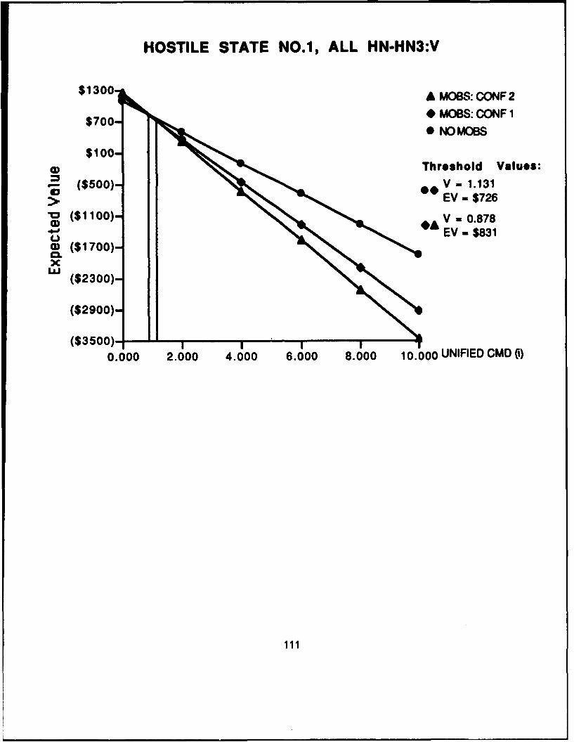
HOSTILE STATE NO.1, ALL HN-HN3:V
$1300. A MOBS: CONF2
7 MOBS: CONF 1* NOMOBS
$1oo-
CD Threshold Values:
$ 500)- eV - 1.131EV - $726
•0 ($1100)- V - 0.878EV - $831cp ($1700)-
x"w ($2300)-
($2900)-
($3500)- -
0.000 2.000 4.000 6.000 8.000 10 .0 0 0 UNIFIED CMD(i)
111
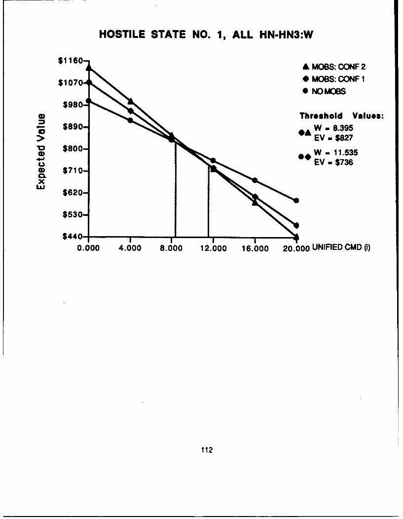
HOSTILE STATE NO. 1, ALL HN-HN3:W
$1160 A MOBS: CONF 2
$1070 * MOBS: CONF 1* NOMOBS
$980iw Threshold Values:
w $890-* W - 8.395>• •&EV - $827V $800i .9
S $800- W - 11.535EV -$736
CD $710-x
$620-
$530-
$440- T
0.000 4.000 8.000 12.000 16.000 20.000 UNIFIED CMD()
112

LEL 1.00 274 o1030 I 161 2740.01 r 2 274
0.00 1030I 1030 0 0'.3 I i I I I
L 0.33 30B 1090 782 256 - -0.1 106 '.4 433i i .6
0.17 1030 10• 0 0 132 -
LEVL'I. .5B 410 1030 ao0 233 - -
0.2 No '.6 - - 64 7934
0.42 190 loo- 0 45 -'s 7 I I I I I
LEM 0.50 512 100 578 255 - -
0.3 106 r. B3020.50 1030o 1090 0 546 ___
I LVE 0.33 649 1090 441 215o0.39 0M r 106 944
L 0.67 1030 1030 0 723
;w rrI I-
LEVEL 1.00 299 1192 8,2 2990.04 106 r 12 299
0.00 1116 1192 76 0r. 13
LE'VEL 0.32 334 1132 853 3060.12 106 r 1439
0.03 1116 1132 76 933r. 15
WtnEED LEVEL 0.67 466 1192 726 310c O l 0.21 Ns .r 16 694 7B2
0.33 1146 1192 46 31346 r 17
LEVEL. 0.58, 530 1132 612 3330.23 106B r 13 821
0.42 1153 1192 34 484r. 13
LEVEL 0.42 732 1192 460 3040.35 10 6 r2 9
05.51 1173 1192 13 6B6
pi - r 21
LEVEL 1.00 314 1261 947 3140.05 H06 r 22
0.00 1130 1261 131 a.r 23
LEVEL 0.92 343 1261 913 3190.13 106 r.2441
0.03 1130 1261 131 49r.25
SLEVEL 0.67 477 1261 7B5 3170.23 06 r 26- 704 790
0.33 1157 1261 105 337r. 27
LEVEL 0.53 605 1261 656 3520.26 106 '.r23 4
0.42 1133 1261 78 434• 1S r 29
LEVEL 0.42 766 1261 494 3190.33 106 r30 II 1026'.3
0.53 1209 1261 52 707
113

[HSTILE STATE NO. 1 COWD HOST NATIONS W/OUT .H3
ANNUAL COSTS OWT (, in ) ily DE PEA & TOTALI
______ ______ 1090
'S O h/ $36.75 / $65.00 1 107W ULTMIS WA $66.25 $105.00 $171.25
NOTE: Proanmaro cost for MOBS ovw 20 YomEOIXVALE04T CUBOC FEET (hn mkx NETWORKiLATGOY L. CAGOID. CAG I ER TOTAL VALUE
1IS266.376 1 55
ObS:STOL 2.278 3.582 D.086 5.946 7&M.2S MULTMIS 4.556 6.098 0.173 10.83271 12
CONFLICT LEVEL PROBABILITY HNS PROBABUITY TAU PROBAEIUTYCONFLICT MOBS CONFIGURATION MOBS CONFIGURATION MOBS CONFKWIRATION
LEVEL NONE STOL MULTUIS NONE STOL MULTMS NONE STOL MULTMSLEVEL 1 0.01 0.04 0.05 1.00 1.00 1.00 1 1 1LEVEL 2 0.1 0.12 0.13 0.83 0.92 0.92 1 1 1LEVEL 3 0.2 0.21 0.23 0.58 0.67 0.67 1 0.6 0.8LEVEL 4 0.3 0.28 0.26 0.50 0.58 0.58 1 0.45 0.6LEVEL 5 0.39 0.35 0.33 0.33 0.42 0.42 1 0.25 0.4CHEcK 1 1 1
W= 10V= 1
RESLLTS BY DECISION AND CONFLICT LEVEL CJ HNS FNALEVEL1 LEVEL2 LEVEL3 LEVEL4 LEVEL5 PRO RESUL
MOBS 273.62 438.46 694.14 801.97 943.74 0.49 794.06T299.43 398.90 693.50 821.28 989.63 0.60 781.81T 314.05 413.52 703.91 846.46 1025.79 0.61 789.95
114

COMBED HOST NATION DATA CObPLATION
COSTS EC" NV
1 225 14 12
4N2 865 252 43
4N3 0 0 0OTAL 1090 266 55
PHNS ECF 816J
SPROBABILITY OF SUPPORT COMPLATION __T' COMPLATIONNONE WPROB STOL. WPROB MM WPROB TAU
1.00 0.16 1.00 0.16 1.00 0.16 134 1.001.00 0.84 1.00 0.84 1.00 0.84 682 1.000.00 0.00 0.00 0.00 0.00 0.00 0 0.00
1.00 1.00 816
1.00 0.16 1.00 0.16 100 2 0.16 134 1.000.80 0.67 0.90 0.75 0.90 0.75 648 0.95
0.00 0.00 0.00 0.00 000 0.00 0 0.000.83 0.62 0.92•82
1.00 0.16 1.00 0.16 1.00 0.16 134 1.000.50 0.42 0.60 0.50 0.60 0.50 546 0.800.00 0.00 0.00 0.00 0.00 0.00 0 0.00
S~0.58 0•--.67 0•---- .67 68071.00 0.16 1.00 0.16 1.00 0.16 134 1.000.40 0.33 0.50 0.42 0.50 0.42 443 0.650.00 0.00 0.00 0.00 0.00 0.00 0 0.00
1.00 0.16 1.00 0.16 1.00 0.16 134 1.000.20 0.17 0.30 0.25 0.30 0.25 307 0.450.00 0.00 0.00 0.00 0.00 0.00 0 0.00
0.1 0.42 0.42 441
115

INITIAL DISTRIBUTION LIST
No. Copies
1. Defense Technical Information Center 2Cameron StationAlexandria, VA 22304-6145
2. Library, Code 0142 2Naval Postgraduate SchoolMonterey, CA 93943-5002
3. Defense Logistics Studies Information Exchange 2U.S. Army Logistics Management CenterFt. Lee, VA 23801
4. Mobile Support Systems Program Office (Code 1235)Carderock Division, Naval Surface Warfare CenterAttn: Keith McAllisterBethesda, MD 20084-5000
5. Professor Kneale T. Marshall Code OR/Mt 3Department of Operations ResearchNaval Postgraduate SchoolMciterey, CA 93943-5000
6. Commander Barbara Y. Marsh-Jones OR/MjDepartment of Operations ResearchNaval Postgraduate SchoolMonterey, CA 93943-5000
7. Professor David A. Schrady Code OR/SoDepartment of Operations ResearchNaval Postgraduate SchoolMonterey, CA 93943-5000
8. Commander Craig TurleyN-402DDepartment of NavyWashington, DC 20350-2000
9. Lieutenant Robert A. Reifenberger 12225 61*1 NorthSt. Petersburg, FL 33710
116