naval postgraduate school will achieve a warship design that effectively links the combat system and...

NAVAL

POSTGRADUATE

SCHOOL

MONTEREY, CALIFORNIA

THESIS

Approved for public release; distribution is unlimited

ESTIMATING PRODUCTION COST WHILE LINKING COMBAT SYSTEMS AND SHIP DESIGN

by

Jeffrey Lineberry

December 2012

Thesis Advisor: Daniel Nussbaum Second Reader: Eugene Paulo

THIS PAGE INTENTIONALLY LEFT BLANK

i

REPORT DOCUMENTATION PAGE Form Approved OMB No. 0704-0188Public reporting burden for this collection of information is estimated to average 1 hour per response, including the time for reviewing instruction, searching existing data sources, gathering and maintaining the data needed, and completing and reviewing the collection of information. Send comments regarding this burden estimate or any other aspect of this collection of information, including suggestions for reducing this burden, to Washington headquarters Services, Directorate for Information Operations and Reports, 1215 Jefferson Davis Highway, Suite 1204, Arlington, VA 22202-4302, and to the Office of Management and Budget, Paperwork Reduction Project (0704-0188) Washington DC 20503.

1. AGENCY USE ONLY (Leave blank)

2. REPORT DATE December 2012

3. REPORT TYPE AND DATES COVERED Master’s Thesis

4. TITLE AND SUBTITLE Estimating Production Cost while Linking Combat Systems and Ship Design

5. FUNDING NUMBERS

6. AUTHOR Jeffrey Lineberry

7. PERFORMING ORGANIZATION NAME(S) AND ADDRESS(ES) Naval Postgraduate School Monterey, CA 93943-5000

8. PERFORMING ORGANIZATION REPORT NUMBER

9. SPONSORING /MONITORING AGENCY NAME(S) AND ADDRESS(ES) Office of Naval Research, ONR 334 875 N. Randolph Street, Suite 1425 Arlington, VA 22203-1995

10. SPONSORING/MONITORING AGENCY REPORT NUMBER

11. SUPPLEMENTARY NOTES The views expressed in this thesis are those of the author and do not reflect the official policy or position of the Department of Defense or the U.S. Government. IRB Protocol number ______N/A______.

12a. DISTRIBUTION / AVAILABILITY STATEMENT Approved for public release, distribution is unlimited

12b. DISTRIBUTION CODE A

13. ABSTRACT (maximum 200 words)

In a Naval International Cooperative Opportunities in Science & Technology Program (NICOP) initiative, the Office of Naval Research (ONR) is investigating whether an emphasis on the utilization of computer simulation and combat modeling will achieve a warship design that effectively links the combat system and the ship design. A success in this effort will result in an enhancement to the ship’s combat mission effectiveness while providing real-time estimates of the associated production cost.

This thesis addresses the cost estimation portion of the various models and simulations associated with the NICOP initiative, with a focus on Offshore Patrol Vessels (OPVs). This thesis identifies the historical and current ship production costs of OPVs that are used for various combat missions. This study supports the NICOP initiative by providing a foundation for further investigation into the framework necessary to provide more accurate cost estimates. This is accomplished within the trade space of the naval architecture developed through the application of Model Based System Engineering (MBSE). The development of a cost model for the NICOP initiative is used as a framework to explain the cost estimating approach process for future MBSE designs. The model is then used to compare to the base model developed by the Italians.

14. SUBJECT TERMS Offshore Patrol Vessel, Model Based System Engineering, Production Cost Estimate

15. NUMBER OF PAGES

83

16. PRICE CODE

17. SECURITY CLASSIFICATION OF REPORT

Unclassified

18. SECURITY CLASSIFICATION OF THIS PAGE

Unclassified

19. SECURITY CLASSIFICATION OF ABSTRACT

Unclassified

20. LIMITATION OF ABSTRACT

UU

NSN 7540-01-280-5500 Standard Form 298 (Rev. 2-89) Prescribed by ANSI Std. 239-18

ii


iii

Approved for public release, distribution is unlimited

ESTIMATING PRODUCTION COST WHILE LINKING COMBAT SYSTEMS AND SHIP DESIGN

Jeffrey Lineberry Lieutenant, United States Navy

B.B.A., Saint Edward’s University, 2003

Submitted in partial fulfillment of the requirements for the degree of

MASTER OF SCIENCE IN OPERATIONS ANALYSIS

from the

NAVAL POSTGRADUATE SCHOOL December 2012

Author: Jeffrey Lineberry

Approved by: Daniel A. Nussbaum Thesis Advisor

Eugene Paulo Second Reader

Robert F. Dell Chair, Department of Operations Research

iv


v

ABSTRACT

In a Naval International Cooperative Opportunities in Science & Technology Program

(NICOP) initiative, the Office of Naval Research (ONR) is investigating whether an

emphasis on the utilization of computer simulation and combat modeling will achieve a

warship design that effectively links the combat system and the ship design. A success in

this effort will result in an enhancement to the ship’s combat mission effectiveness while

providing real-time estimates of the associated production cost.

This thesis addresses the cost estimation portion of the various models and

simulations associated with the NICOP initiative, with a focus on Offshore Patrol Vessels

(OPVs). This thesis identifies the historical and current ship production costs of OPVs

that are used for various combat missions. This study supports the NICOP initiative by

providing a foundation for further investigation into the framework necessary to provide

more accurate cost estimates. This is accomplished within the trade space of the naval

architecture developed through the application of Model Based System Engineering

(MBSE). The development of a cost model for the NICOP initiative is used as a

framework to explain the cost estimating approach process for future MBSE designs.

The model is then used to compare to the base model developed by the Italians.

vi


vii

TABLE OF CONTENTS

I. INTRODUCTION........................................................................................................1 A. OVERVIEW .....................................................................................................1 B. COST ESTIMATING METHODOLOGY ...................................................2 C. RESEARCH QUESTIONS .............................................................................4 D. CHAPTER SUMMARY ..................................................................................4

II. PROJECT BACKGROUND AND LITERATURE REVIEW ................................5 A. APPLYING MBSE TO DECISION MAKING ............................................5

1. Introduction to MBSE .........................................................................5 2. Applying MBSE in Trade Space Analysis .........................................6

B. CURRENT PROJECT PROGRESS..............................................................8 C. COST ESTIMATING NAVAL SHIP DESIGNS..........................................9

1. Estimating Construction Costs in the Design Phase .........................9 2. Estimating Costs as a Function of Performance Levels .................10

III. DETAILED METHODOLOGY...............................................................................11 A. COLLECTING AND ORGANIZING THE DATA ...................................11

1. Jane’s Fighting Ships .........................................................................11 2. NAVSEA 05C Production Cost Data on USCG’s 270’ WMEC ....13 3. Dr. Nussbaum’s OPV Weight Data ..................................................14

B. NORMALIZING THE DATA ......................................................................14 1. Analyzing Factors ..............................................................................14 2. Units of Measure and Conversions ...................................................15 3. Normalization .....................................................................................17

C. REGRESSION METHODOLOGY .............................................................17 a. Prob > │t│ ...............................................................................18 b. Prob > F ...................................................................................18 c. and adjusted ................................................................18 d. CI..............................................................................................18

IV. COST ANALYSIS .....................................................................................................21 A. PRODUCTION COST ESTIMATION DASHBOARD .............................21

1. Development .......................................................................................21 B. ANALYZING THE DATA ...........................................................................24

1. Jane’s Fighting Ships .........................................................................24 2. NAVSEA 05C Production Cost Data on USCG’s 270’ WMEC ....28 3. Dr. Nussbaum’s OPV Weight Data ..................................................29

C. DISTRIBUTION ANALYSIS .......................................................................30 D. REGRESSION ANALYSIS ..........................................................................31

1. Multicollinearity .................................................................................31 2. Overall Length ...................................................................................33 3. Overall Beam ......................................................................................36 4. Full Load Displacement .....................................................................38 5. Light Ship Weight ..............................................................................40

viii

E. UTILIZATION OF THE DASHBOARD ....................................................42 1. Royal Thai Navy CDR Peerapong’s MIO Simulation ....................42 2. LT Joe Ashpari of the United States Navy ......................................46 3. LT Jason McKeown of the United States Navy ..............................49

F. COMPARATIVE ANALYSIS ......................................................................50

V. SUMMARY AND CONCLUSION ..........................................................................53 A. UTILIZATION IN NICOP INITIATIVE ...................................................53 B. THE COST MODEL FRAMEWORK ........................................................53

1. How to Apply this to Future MBSE Designs ...................................53 C. IMPROVEMENTS FOR BETTER ANALYSIS ........................................56

1. Propulsion Systems ............................................................................56 2. Hull Material ......................................................................................56 3. Complexity Models ............................................................................56

D. USING THIS MODEL FOR NEXT SHIP–BIGGER SHIP–POSSIBLY LSDX ..........................................................................................56

LIST OF REFERENCES ......................................................................................................59

INITIAL DISTRIBUTION LIST .........................................................................................63

ix

LIST OF FIGURES

Figure 1. Ship Cost Estimation Methods based on Design Maturity and Program Life Cycle (D. Nussbaum, OA4702, January 2012, from Naval Sea Systems Command Cost Engineering and Industrial Analysis Division, 2008). .................................................................................................................3

Figure 2. MBSE Design for PRONTO/ASNET Project (From A. MacCalman & E. Paulo, unpublished slide, November 2011) .......................................................7

Figure 3. NPS Dashboard for PRONTO/ASNET Project (P. Beery & P. Roeder, unpublished dashboard, June 7, 2012). ..............................................................9

Figure 4. August Westland Lynx (From aviationsmilitaires.net) ....................................16 Figure 5. Marte [Left] (From MBDA Missile Systems),Exocet [Right](From

Surbrook-Devermore) ......................................................................................16 Figure 6. Italian Ship 35mm Gun (From navweaps.com). ..............................................16 Figure 7. USCG Eagle Eye VUAV (From Wikipedia). ..................................................17 Figure 8. Opening, Input, page of the Dashboard ...........................................................22 Figure 9. Output page of the Dashboard .........................................................................22 Figure 10. Synthesis Flow via Distributional and Regression Analysis ...........................24 Figure 11. Distributions of OPV Factors...........................................................................25 Figure 12. Distribution of Crew Complement based on Number of On-Board

Helicopter(s). ...................................................................................................27 Figure 13. One-way ANOVA of Crew Complement by Number of On-Board

Helicopter(s) ....................................................................................................27 Figure 14. Distribution of Weight (lbs) based on single digit SWBSE (After

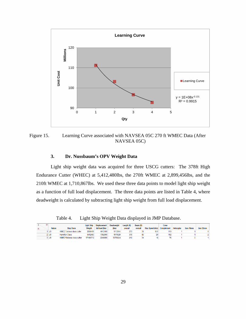
NAVSEA 05C) ................................................................................................28 Figure 15. Learning Curve associated with NAVSEA 05C 270 ft WMEC Data (After

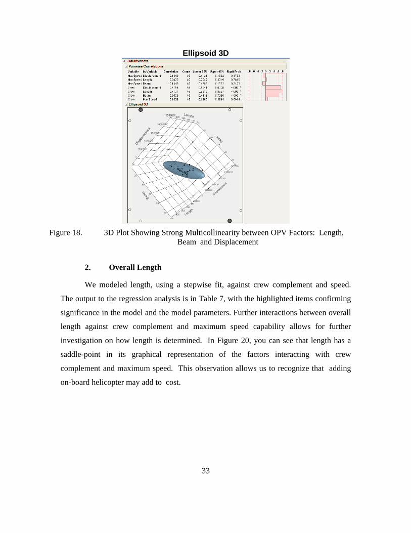
NAVSEA 05C) ................................................................................................29 Figure 16. More Detailed Distribution Analysis of Crew Complement ...........................30 Figure 17. Graphical Representation of the Correlation between OPV factors. ...............32 Figure 18. 3D Plot Showing Strong Multicollinearity between OPV Factors: Length,

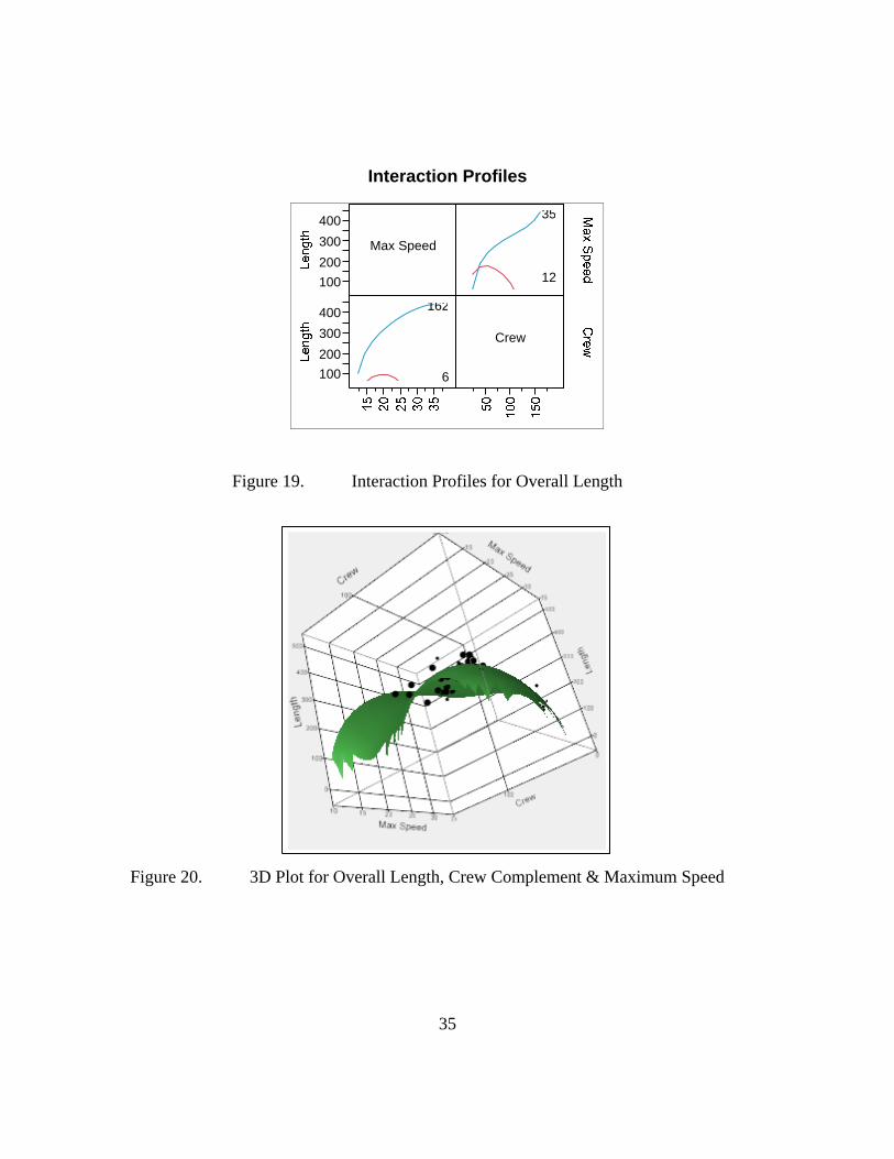
Beam and Displacement .................................................................................33 Figure 19. Interaction Profiles for Overall Length ............................................................35 Figure 20. 3D Plot for Overall Length, Crew Complement & Maximum Speed .............35 Figure 21. Regression Plot for Overall Beam ...................................................................36 Figure 22. Regression Plot for Full Load Displacement ...................................................38 Figure 23. Regression Plot for Weight against Displacement...........................................40 Figure 24. Royal Thai Navy CDR Peerapong’s MANA Simulation—depicting a

screenshot of the end-state of a scenario model (Y. Peerapong, Thesis pending publishing, June 2012). ......................................................................46

Figure 25. Line graph of various architectural factors and cost estimates of an OPV with 2 on-board VUAVs as Max Speed Capability goes up. ..........................48

Figure 26. Italian Model Output: Cost Analysis for Different ship solutions (A. Bonvicini, unpublished slide, 2011). ...............................................................51

x

Figure 27. Comparison Graph representing US Cost model against Italian Cost model................................................................................................................52

Figure 28. Depiction of the process flow in developing a MBSE production cost model that changes reflective to changes in combat configurations. (Images from (left to right): navweaps.com, surbrook.devermore.net, mnvdet.com, en.wikipedia.org, military-pilots.blogspot.com, 123rf.com, & all-silhouettes.com). .........................................................................................55

xi

LIST OF TABLES

Table 1. Compiled Ship Data from Jane’s Fighting Ships (After Jane’s Fighting Ships, 2012). ....................................................................................................11

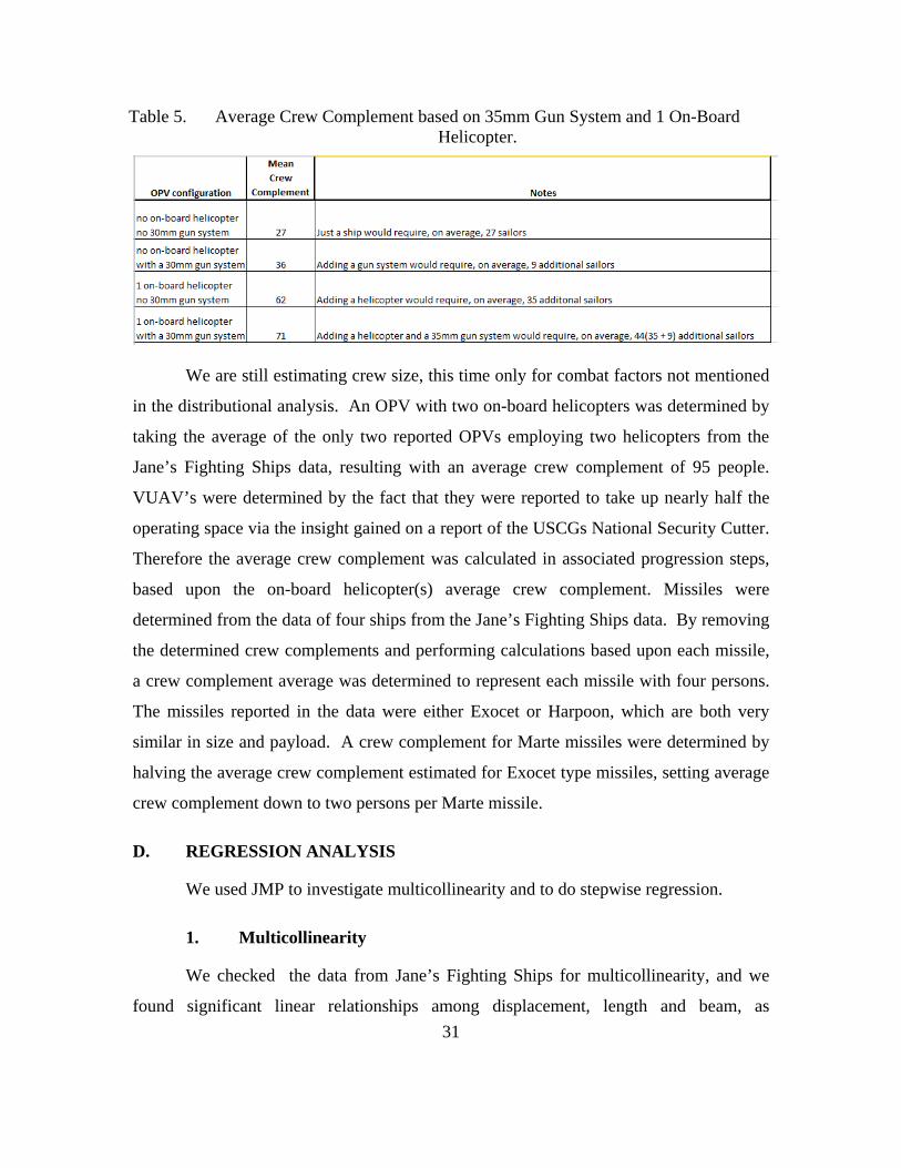
Table 2. SWBSE acquired from NAVSEA data (After NAVSEA 05C). ......................13 Table 3. Light ship weight data in lbs. (After Dr. Nussbaum). ......................................14 Table 4. Light Ship Weight Data displayed in JMP Database. ......................................29 Table 5. Average Crew Complement based on 35mm Gun System and 1 On-Board

Helicopter. ........................................................................................................31 Table 6. Multivariate Correlations of OPV factors. .......................................................32 Table 7. JMP Regression Output for Overall Length. ...................................................34 Table 8. JMP Regression Output for Overall Beam. .....................................................37 Table 9. JMP Regression Output for Full Load Displacement. .....................................39 Table 10. JMP Regression Output for Light Ship Weight ...............................................41 Table 11. Cost Estimates for MIO Simulation Output Analysis ......................................45 Table 12. Cost Estimates for SAR Simulation Output Analysis ......................................48 Table 13. Cost Estimates for ASuW Simulation Output Analysis ..................................50

xii


xiii

LIST OF ACRONYMS AND ABBREVIATIONS

ANOVA Analysis of Variance

AO Area of Operations

ASNET Application System for Naval Evaluation and Testing

ASuW Anti-Surface Warfare

CI Confidence Interval

DOE Design of Experiments

INCOSE International Council on Systems Engineering

JIC Joint Inflation Calculator

MBSE Model Based System Engineering

MIO Maritime Interdiction Operations

MOE Measure of Effectiveness

NAVSEA Naval Sea Systems Command

NCCA Naval Center for Cost Analysis

NICOP Naval International Cooperative Opportunities in Science & Technology Program

NPS Naval Postgraduate School

OMOE Overall Measure of Effectiveness

ONR Office of Naval Research

OPV Offshore Patrol Vessel

PRONTO Partnership for Research on Naval Technology and Operations

SAR Search and Rescue

SEA 05C Cost Engineering and Industrial Analysis Division

SEED Simulation Experiments & Efficient Design

xiv

SWBSE Ship Work Breakdown Structure Elements

USCG United States Coast Guard

VTOL Vertical Takeoff and Landing

VUAV VTOL Unmanned Aerial Vehicle

WHEC High Endurance Cutter

WMEC Medium Endurance Cutter

xv

EXECUTIVE SUMMARY

Historically, the shipbuilding process begins with preliminary planning, followed

by the creation of the ship platform design, with only minimal consideration for combat

effectiveness. This thesis addresses the ability to develop a cost model that estimates

ship production costs as combat effectiveness factors are adjusted in the design trade

space through the application of Model Based System Engineering (MBSE). We build a

cost estimating model that responds in real time to changes in combat systems

configurations, namely ship aviation capabilities (e.g., with or without an on-board

helicopter), armament configurations (e.g., with or without a 35mm gun system), and

maximum speed capabilities.

The Naval Postgraduate School (NPS) Simulation Experiments & Efficient

Design (SEED) Center for Data Farming, in collaboration with Office of Naval Research

(ONR), is supporting the application of an MBSE approach to naval ship design. The

emphasis is placed on advancing the design process within the constructs of the MBSE

design. This thesis focuses on the cost estimation process and how a cost estimate should

be constructed for MBSE projects. The recursive use of a cost estimating process

contributes to the future approach of producing such estimates within the MBSE

paradigm.

For this investigation, we built a cost estimating tool that has the ability to

produce a ship production cost estimate that is dependent on the combat system

configurations. This cost estimating tool allows for further insight on how to develop this

tool for other systems. With a deeper investigation on the make-up of this cost estimating

tool, we are able to investigate the trade space within the MBSE paradigm. This is

accomplished by a focus on the correlation amongst the combat systems and the ship’s

naval architecture.

xvi


xvii

ACKNOWLEDGMENTS

The author would like to thank the following individuals:

In memory of CAPT Alan Goodwin “Dex” Poindexter USN, whose words of

encouragement motivated me to put forth my best effort for this thesis.

Dr. Dan Nussbaum for his exceptional guidance and encouragement as thesis

advisor.

Dr. Eugene Paulo for his outstanding guidance as second reader.

Ms. Kelly Cooper, Mr. Richard Vogelsong, and Mr. David Edwards from ONR

for their overall promotion of the MBSE NICOP project and hosting the NICOP

ASNET/PRONTO Tech Review in West Bethesda, MD.

LTC Alex MacCalman, USA; CDR Doug Williams, USN; CDR Peerapong

Yoosiri, Royal Thai Navy; LT Jason McKeown, USN; LT Joe Ashpari, USN; Mr.

Paul Beery and Mr. Paul Roeder—for their parallel efforts throughout this project.

CDR Andrew Meverden, USCG; CAPT Brad Fabling, USCG; Mr. Geoffrey

Pawlowski, NAVSEA/SPAWAR for providing OPV cost data necessary for the

analysis in this thesis.

LT Jason Fox for his previous efforts on the PRONTO/ASNET project and his

availability via e-mail to answer questions pertaining to his thesis.

Francesco Perra, Natalino Dazzi, Aldo Guagnano, Alessondro Bonvicini and

Massino Paolucci for their combined efforts in developing the Italian model that

was utilized as a baseline for the underlying PRONTO/ASNET project.

Dimitri Mavris, Santiago Balestrini-Robinson, Kelly Griendling, Rebecca

Douglas and Janel Nixon from Georgia Tech for hosting our Atlanta, GA ASNET

NICOP meeting and their contributions towards the project.

xviii

My lovely wife, Crystal Faith, and our wonderful children, Kylar, Courtney,

Bonnie, Dillon, and Jeffrey, for their understanding and support for my efforts

while I was dedicated to this thesis.

1

I. INTRODUCTION

A. OVERVIEW

The complete design of a naval combatant ship is an extraordinarily complex

process. It can take decades for a design to mature from infancy to delivery of the first

ship. Among many problems with this lag is that over 20 years, the requirements that

generated the initial design may be long irrelevant, yet a program may be too “invested”

to simply abandon it. Additionally, over this period of time, cost estimates which had

been deemed “affordable” can evolve into “unaffordable” estimates. Cost estimates must

include not only those aspects related to the ship itself, but life cycle costs and any other

aspects related to total ownership costs. These costs must be estimated by many points

through the design life of the program, in order to determine the best cost versus mission

effectiveness trade-offs.

A team of Naval Postgraduate School (NPS) faculty and students, in collaboration

with other researchers is utilizing Model Based System Engineering (MBSE) in an

approach to develop and demonstrate a methodology to use the output analyses of the

combat systems effectiveness as ship characteristic inputs for the ship design process.

The specific ship being analyzed and designed in this project sponsored by the Office of

Naval Research (ONR) is an Offshore Patrol Vessel (OPV), which serves as an important

naval platform for numerous navies. An important aspect of this broad research is to

examine impacts of combat system technology trade-offs, and include consideration of

cost, risk, and system effectiveness in multiple criteria trade space analysis. Thorough

trade space analysis will result from the linkage of combat system capabilities, ship

design and selection, and cost estimation, through modeling and simulation.

This thesis focuses on the cost estimation aspect of this problem. In this chapter

we provide an introduction of the Naval International Cooperative Opportunities in

Science & Technology Program (NICOP) initiative with some clarification to the concept

of the MBSE design. Current progress is described in relation to the NICOP initiative for

the Partnership for Research on Naval Technology and Operations

2

(PRONTO)/Application System for Naval Evaluation and Testing (ASNET) project.

Focus and clarification for this thesis effort is introduced along with a cost estimating

methodology overview.

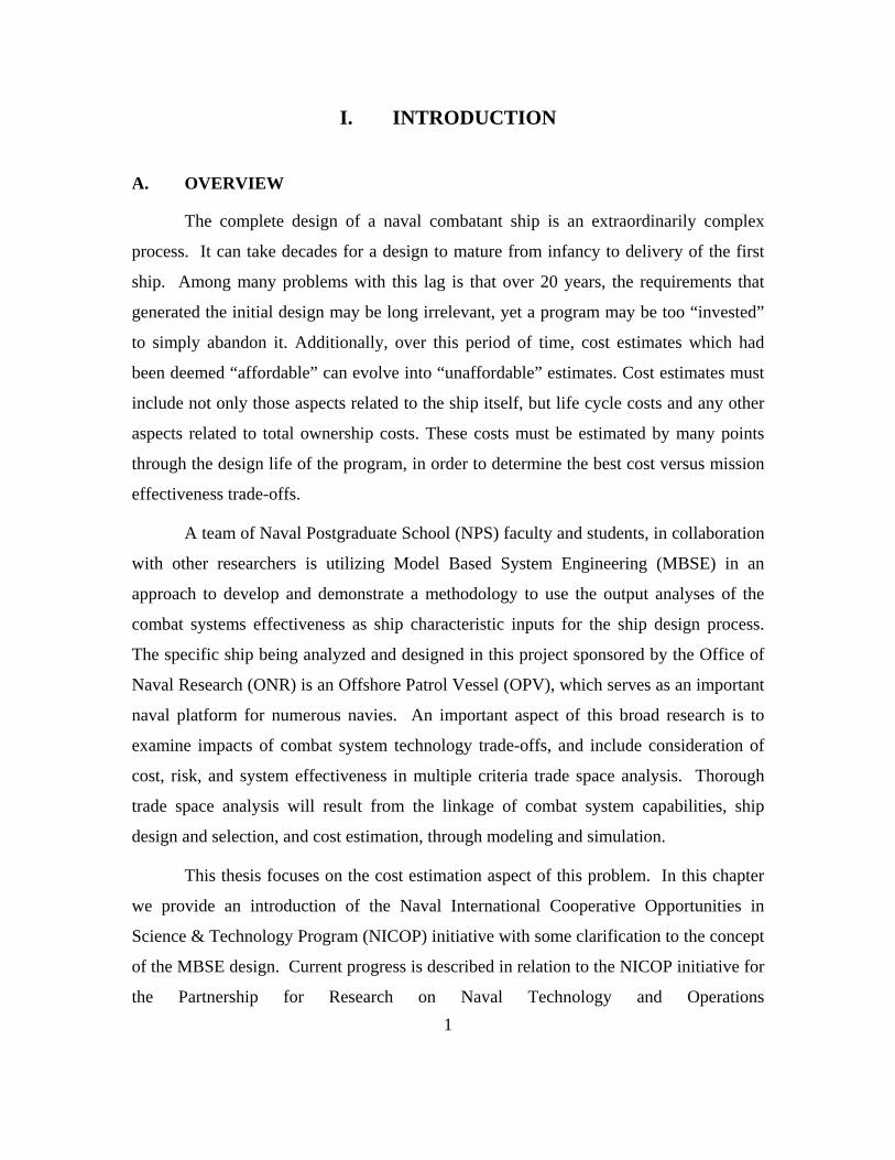
B. COST ESTIMATING METHODOLOGY

The four common methodologies for producing a cost estimate are Analogy,

Expert Judgment, Bottom-Up, and Parametric Models (D. Nussbaum, personal

communication, January 2012). Generally, the Parametric and Analogy methodologies

are preferred during the earlier design phases and planning of the project, since they can

be used in a limited data environment. As the project design matures, additional data will

become available, at which point the Bottom-Up methodology can also be employed.

Once production is initiated, the use of actual costs to estimate future production costs

becomes feasible (D. Nussbaum, personal communication, February 2012). Expert

Judgment, although only as strong as the credibility of the expert and lacking any

statistical measures of goodness, can be applied throughout the system’s life cycle.

Figure 1 shows an association of the preferred estimating methodologies based on the

design maturity. As this thesis addresses the early conceptual design phase of an OPV,

Parametric and Analogy are the cost estimating methodologies of choice.

3

Figure 1. Ship Cost Estimation Methods based on Design Maturity and Program Life Cycle (D. Nussbaum, OA4702, January 2012, from Naval Sea Systems Command

Cost Engineering and Industrial Analysis Division, 2008).

This thesis builds a cost estimating model that is responsive to real time changes

in combat system configurations. This is accomplished by collecting analogous data and

using this data to:

Estimate naval architectural factors (e.g., length, beam, displacement and crew

complement) from combat system configurations (e.g., length as a function of crew

complement and max speed). These relationships are developed in Chapter IV, which is

derivable from full load displacement, as described in Chapter III.

Develop a dollar per pound metric. Since this metric is based on a 4-ship class of

United States Coast Guard (USCG) Medium Endurance Cutter (WMEC), we used a

learning curve to extend this to an n-ship class.

Applying the dollar per pound metric to the light ship weight described in Chapter

III.

4

C. RESEARCH QUESTIONS

Develop a cost model that estimates OPV life cycle costs as a function of the design factors within the MBSE design trade space.

Explain the concepts and development of the life cycle cost model with the purpose of proposing a framework for future cost estimation efforts for the MBSE paradigm.

D. CHAPTER SUMMARY

Chapter I provides an introduction of the concept of the MBSE design paradigm

and a cost estimating methodology overview utilized for the efforts pertaining to this

thesis’ focus. Chapter II provides a deeper insight into the MBSE design concept and

cost estimating pertaining to ship designs and system performance, as well as a

description of how OPVs are being used in naval operations. Chapter III provides a

detailed methodology pertaining to the cost estimating efforts established for the focus of

this thesis. Chapter IV provides a detailed description of the production cost estimating

dashboard developed for this thesis effort, the analysis done to build the production cost

dashboard, and more insight into the use of the dashboard through examples of the

dashboard being utilized to reflect early analysis output from the three simulation models

being developed at NPS. Chapter V provides a summary and conclusion.

5

II. PROJECT BACKGROUND AND LITERATURE REVIEW

A. APPLYING MBSE TO DECISION MAKING

1. Introduction to MBSE

The International Council on System Engineering (INCOSE) defines MBSE as

“the formalized application of modeling to support system requirements, design, analysis,

verification and validation activities beginning in the conceptual design phase and

continuing throughout development and later life cycle phases”(International Council on

System Engineering, 2007). The major distinction of MBSE is that it emphasizes the

models as a foundation for the engineering process, represented as a model-focused

approach to system designs vice the traditional hardcopy design approach. This form of

modeling is possible through the use of computing power (Kleijnen, Sanchez, Lucas &

Cioppa, 2005). The ability to simulate the operations and conditions of the system being

engineered is a possibility which allows for the MBSE method to test a system before the

development phase has begun.

The origin of SE can be traced to Wayne Wymore’s mathematical contributions

and promotional efforts that led to the recognition of SE as a science (The University of

Arizona, 2004). Wymore’s book entitled, Model-Based Systems Engineering: An

Introduction to the Mathematical Theory of Discrete Systems provides an early basis for

the conceptualization of SE driven by a model-based framework (Estefan, 2008). MBSE

has evolved over the past fifteen years, contributing to accuracy in engineering

development and a greater reliance on a wide spectrum of methodologies, processes, and

tools (Tepper, 2010). MBSE identifies the driving force of the system, through the effort

of models, to analyze and communicate the properties of the system to the engineer.

Although there have been many successfully validated projects completed through the

use of MBSE, e.g., NASA space suit design, there have also been failures (Cadova,

Kovich, & Sargusingh, 2012).

6

2. Applying MBSE in Trade Space Analysis

This thesis supports an overall NPS effort to improve ship architecture through an

understanding of the needed operational effectiveness. The ship platform that serves as

the focus for the wide range of our analysis is the OPV. Many navies use OPVs for more

than one mission, so the effectiveness of design constructs against the ability to perform

several of these missions is addressed. The OPVs in this project are classified by their

missions; namely Maritime Interdiction Operations (MIO), Search and Rescue (SAR) and

Anti-Surface Warfare (ASuW). When decision makers have the responsibility to select a

design, they often do not have the engineering subject matter expertise in order to make

an educated and well-informed selection. Simulation and modeling done in the design

phase can help to understand how mission effectiveness depends on various engineering

factors. These Measures of Effectiveness (MOEs) can be aggregated to represent a single

Overall Measure of Effectiveness (OMOE) to decide which ship designs allow the ship to

perform as required.

Ensuring the model is able to easily communicate to the decision makers, the

creation of a user-friendly computer generated program that involves user interaction,

often termed as a ‘dashboard’, may be utilized. The dashboard should illuminate the

trade space and can further simplify the decision maker’s duties, giving them a gauge to

pose their decision upon by facilitating analysis. The MOEs are critical since they will be

the driving force for the decision maker’s choices. The utilization of polynomial meta-

model functions acting as simulation model surrogates allows exploration within the

MBSE design trade space (A. MacCalman, personal communication, May 10, 2012).

Linking the operational environment to the simulation models allows for the development

of critical MOEs that determine the operational space. On the other side of the spectrum

are the naval architectural design parameters that make up the physical space. Both are

conducive of the operational requirements that pertain to both ship development and

combat effectiveness.

Figure 2 depicts a dynamic process of the MBSE design concept for this project.

The left side of the figure describes the factors and requirements that are made up of real-

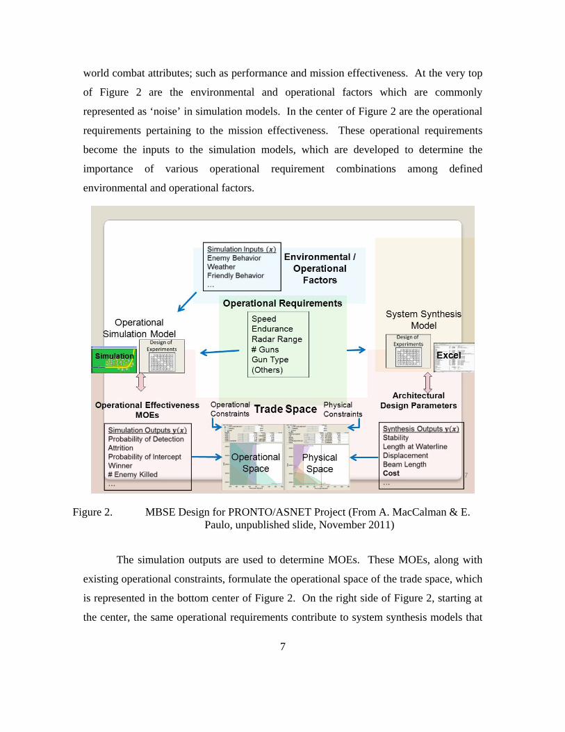
7

world combat attributes; such as performance and mission effectiveness. At the very top

of Figure 2 are the environmental and operational factors which are commonly

represented as ‘noise’ in simulation models. In the center of Figure 2 are the operational

requirements pertaining to the mission effectiveness. These operational requirements

become the inputs to the simulation models, which are developed to determine the

importance of various operational requirement combinations among defined

environmental and operational factors.

Figure 2. MBSE Design for PRONTO/ASNET Project (From A. MacCalman & E. Paulo, unpublished slide, November 2011)

The simulation outputs are used to determine MOEs. These MOEs, along with

existing operational constraints, formulate the operational space of the trade space, which

is represented in the bottom center of Figure 2. On the right side of Figure 2, starting at

the center, the same operational requirements contribute to system synthesis models that

8

define the architectural design parameters. With the consideration of known physical

constraints, theses architectural design parameters mold the physical space. Through the

utilization of computing power and scientific design, linking the combat system

capabilities and ship design is accomplished by developing an OMOE that defines

operational performance. The operational performance is linked to architectural design

parameters to reveal acceptable boundaries within the various factors that make up the

architecture of the ship. To simplify this concept, the development of a dashboard is used

to represent the OMOE and associated architectural considerations.

B. CURRENT PROJECT PROGRESS

NPS’s contribution to the project is incorporating naval operational insights into

the simulations analysis, to include a focus on cost estimation. Three simulation models

are being built to add more insight into the naval tasks they represent, and additional

work is being done to develop a dashboard, which serves as a dynamic decision tool.

Royal Thai Navy CDR Yoosiri Peerapong has developed a MIO simulation

utilizing MANA, which defines the mission more accurately. His main objectives were

identifying significant parameters affecting the MIO mission along with the additional

analysis of the improvement capabilities of a Vertical Takeoff and Landing (VTOL)

Unmanned Aerial Vehicle (VUAV) (Yoosiri, 2012).

LT Joseph Ashpari is investigating the SAR mission with the purpose of

investigating the importance based on factors of OPV maximum speed, employment of a

combination of helicopters and VUAVs on board (Ashpari, 2012)

LT Jason McKeown has developed an ASuW simulation utilizing MANA. An

advanced model is being developed in order to more realistically represent real-world

implications, such as clarifying kill probabilities of armament aboard the ship, various

sizes and amount of armament, programming the small attack boats to have intelligent

deterrence capabilities, the ability to increase the number of small boat attackers and the

development of a more realistic noise component by including friendly and neutral boats

in the operating area (McKeown, 2012).

9

Mr. Paul Beery and Mr. Paul Roeder have collaborated on the development of a

dashboard that allows exploration of the operational and synthesis meta-models,

involving value modeling that assesses the three operational scenarios in relation to each

other. This dashboard is visually represented by an ability to move crosshairs within

either space to explore the synthesis meta-model that illustrates both the operational and

physical aspects of the trade space as depicted in Figure 3. This dashboard has integrated

the cost estimating parametric equations, representative of this thesis effort (P. Beery &

P. Roeder, unpublished dashboard, 2012).

Figure 3. NPS Dashboard for PRONTO/ASNET Project (P. Beery & P. Roeder, unpublished dashboard, June 7, 2012).

C. COST ESTIMATING NAVAL SHIP DESIGNS

1. Estimating Construction Costs in the Design Phase

Understanding how the design affects costs is crucial to any project. With the

onset of new technologies and increasing labor and material costs, costs overruns are still

a common phenomenon (Arena, 2006). The more complex a ship is, the more difficult it

10

is to trace the design costs of the ship. This is an important factor for knowing where to

budget investment without affecting other attributes in the construction process. The

ability to manage cost information is crucial, although it does not give the ability to

identify an accurate budget proposal before the production phase of the development life

cycle (Fischer & Holbach, 2011). The early stages of ship design are very complex,

where many decisions must be made with a minimal amount of knowledge and a great

amount of risk, especially when new concepts are introduced (Hockberger, 1996).

Producing a cost estimate during this early design stage has important consequences since

this is where a ship construction budget will be imposed, and the decision of where to

allocate money will be implemented.

2. Estimating Costs as a Function of Performance Levels

Estimating costs for levels of performance during the design phase is rarely done.

Rather, naval architectural design parameters are the usual cost drivers, so that the ability

to identify the critical attributes affecting the system and its interactive flow is a proposed

step towards this idea of costing performance (Brown & Salcedo, 2003). Linking

effectiveness to design is the concept encapsulated in the MBSE paradigm (Piaszczyk,

2011).

11

III. DETAILED METHODOLOGY

In this chapter we describe the data obtained for the cost estimating effort and the

data analysis methodology. Historically, ship weight and ship costs are positively

correlated, and regression analyses have been used to model their relationship. In

particular, light ship weight is a good predictor of costing “simple” ships which have

historical antecedents (Miroyannis, 2006). By “simple”, Miroyannis means single-hull

ships such as OPVs, and we apply this weight based approach to estimating the costs of

OPVs.

A. COLLECTING AND ORGANIZING THE DATA

Data on OPVs were obtained from Jane’s Fighting Ships, Dr. Dan Nussbaum and

Naval Sea Systems Command (NAVSEA) Cost Engineering and Industrial Analysis

Division (SEA 05C). We describe these datasets below.

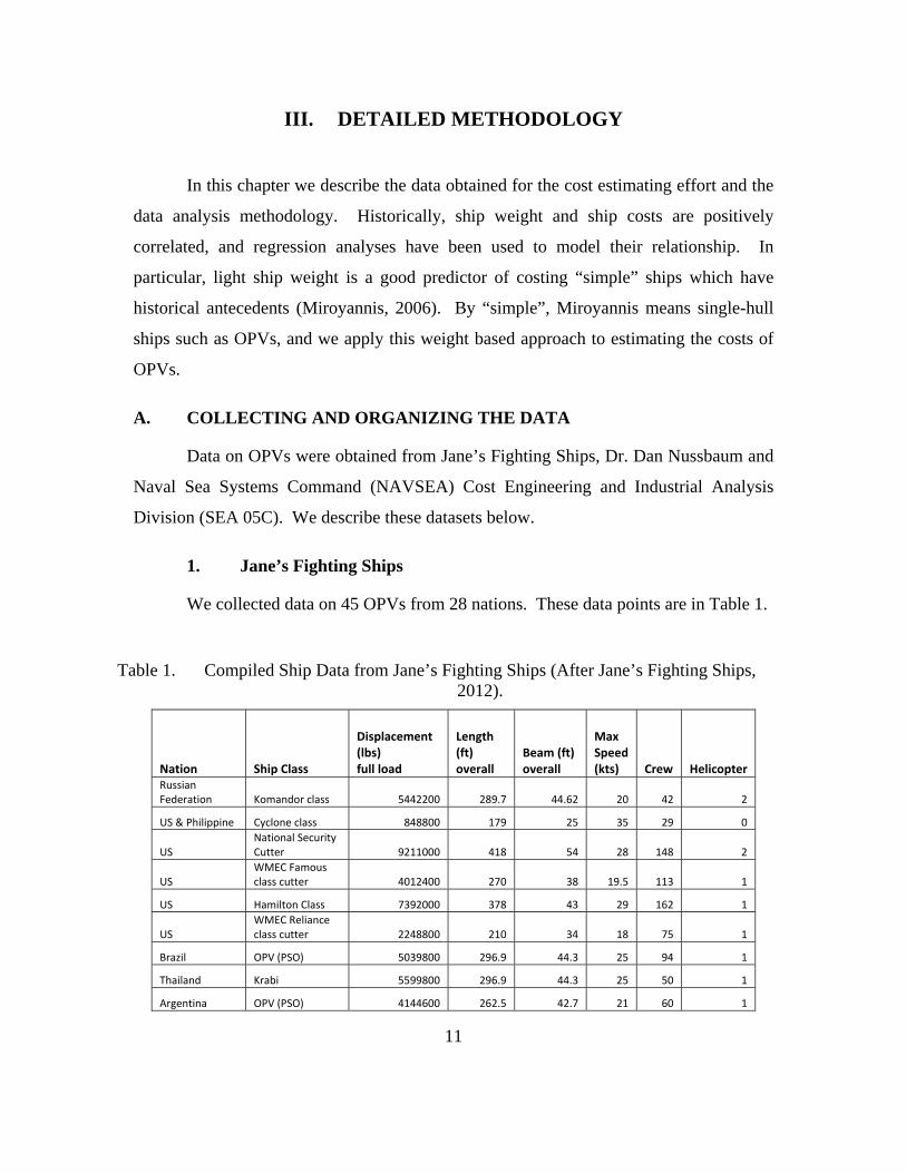
1. Jane’s Fighting Ships

We collected data on 45 OPVs from 28 nations. These data points are in Table 1.

Table 1. Compiled Ship Data from Jane’s Fighting Ships (After Jane’s Fighting Ships, 2012).

Nation Ship Class

Displacement (lbs) full load

Length (ft) overall

Beam (ft)overall

Max Speed (kts) Crew Helicopter

Russian Federation Komandor class 5442200 289.7 44.62 20 42 2

US & Philippine Cyclone class 848800 179 25 35 29 0

US National Security Cutter 9211000 418 54 28 148 2

US WMEC Famous class cutter 4012400 270 38 19.5 113 1

US Hamilton Class 7392000 378 43 29 162 1

US WMEC Reliance class cutter 2248800 210 34 18 75 1

Brazil OPV (PSO) 5039800 296.9 44.3 25 94 1

Thailand Krabi 5599800 296.9 44.3 25 50 1

Argentina OPV (PSO) 4144600 262.5 42.7 21 60 1

12

Nation Ship Class


Length (ft) overall

Beam (ft)overall


Montenegro Kotor class 4188800 317 42 27 110 1

Taiwan PSO 4640800 323 43 24 68 1

Turkey Dost class 3807400 291 40 22 65 1

Spain Meteoro class 6261200 308 47 20.5 50 1

Colombia PSO 3798600 264 43 20 40 1

India, Mauritius Vikram class 2866000 243 37 22 84 1

India Vikram class 2742600 243 37 22 107 1

Venezuela Guaiqueri class 5227200 324.46 44.62 24 60 1

United Kingdom River Class 3807400 261.65 44.62 20 66 1

United kingdom Modified River Class 4138000 267.9 44.62 20 77 1

Spain Alboran class 4398200 218.18 36.09 13 53 1

Portugal Viana Do Castelo 4118200 272.64 42.29 20 43 1

Malta Diciotti class 879600 175.2 26.57 23 29 1

Spain Serviola class 2568400 225 34 19 56 1

Malaysia Langkawi class 2912400 246.06 35.43 22 86 1

Turkey Milgem class 4479800 325 47 29 106 1

France Gowind corvette 3307000 285.43 42.65 21 59 1

France Florẻal class 6607200 306.76 45.93 20 131 1

Italy Cassiopea class 3304800 261.81 38.71 20 70 1

US Asheville 527000 164.37 23.95 35 28 0

US Sentinel 791400 153.22 25.26 28 22 0

US Island 377000 109.91 21 29 18 0

Latvia Valpas 1221400 159.1 27.9 15 18 0

Iraq OPV (PSO) 3086400 197 37 16 42 0

Finland Improved Tursas class 2464800 190 36 15 30 0

Finland Tursas class 2799800 202 33 14 32 0

Taiwan PBO 4085200 277 41 20 40 0

Lebanon PSO 584200 143 27.9 25 6 0

India Rani Abbakka class 615000 168 27.6 34 35 0

Venezuela Constitución class 381400 121 23.3 31 24 0

Trinidad, Tobago PBO 447600 151.9 29.86 20 19 0

Sri Lanka Jayesagara Class 738600 130.58 22.97 15 56 0

Taiwan WPBO 1878400 168.96 27.56 16 22 0

Taiwan WPSO 2522000 193.24 31.5 16 25 0

Taiwan WPSO 1567400 201.44 31.17 30 33 0

13

Nation Ship Class


Length (ft) overall

Beam (ft)overall


Spain Pescalonso class 4706800 222.44 36.09 12 42 0

2. NAVSEA 05C Production Cost Data on USCG’s 270’ WMEC

NAVSEA 05C provided cost data for the first four ships in production of the

USCGs 270ft WMEC. The data consisted of weight, total man-hours, and total material

dollars for each of the Ship Work Breakdown Structure Elements (SWBSE) in Table 2.

All data was reported in US FY77$ and we normalized it to US FY12$.

Table 2. SWBSE acquired from NAVSEA data (After NAVSEA 05C).

100—Hull Structure

200—Propulsion Plant

300—Electrical Plant

400—Command and Surveillance

500—Auxiliary Systems

600—Outfit and Furnishings

700—Armament

800—Integration/Engineering

900—Ship Assembly and Support Services

The data obtained of the 270ft WMEC was obtained from NAVSEA 05C who

informed us that these data are competition sensitive. Therefore these data are not

included in this written thesis. It may be acquired from NPS Operations Research

Professor, Dr. Dan Nussbaum, on a case-by-case basis.

14

3. Dr. Nussbaum’s OPV Weight Data

Light ship weight data in short tons (US) was acquired from Dr. Nussbaum for

three USCG cutters. These data are described in Table 3.

Table 3. Light ship weight data in lbs. (After Dr. Nussbaum).

B. NORMALIZING THE DATA

1. Analyzing Factors

Naval architecture involves many factors, but our focus on a single type of ship, a

single hull OPV, permits us to narrow our considerations to four factors: displacement,

length, beam, and crew complement.

Displacement is a confusing part of naval architecture because of the many

different definitions that involve the word “displacement.” In this thesis, we use full load

displacement, which is defined in detail in chapter IV. Since we are dealing with a single

hull ship, we know we will be relying on the displacement attributed to weight support

(Tupper & Muckle, 1996). Since light ship weight can be modeled as a function of full

load displacement (see page 40) it is sufficient for our purposes to collect full load

displacement data. Full load displacement is reported in datasets such as Jane’s Fighting

Ships.

Flotation and stability requirements impose hull-development relationships on

length and beam, which in turn constrain the architectural volume of a ship, its on-load

weight capacity, crew size, and other associated design parameters (Tupper & Muckle,

1996).

Since each piece of equipment has an associated crew complement, attention must

be placed on the volume requirements associated with the mission of the ship.

15

2. Units of Measure and Conversions

We used the following definitions, conversions, and combat system identities for

this thesis:

Light ship weight, measured in pounds, is the weight of the ship without payload.

That is, light ship weight = displacement (full load) – total deadweight including payload,

ballast water, provisions, fuel, lubricants, water, persons, and personal affects

(Schneekluth, Knovel, & Bertram, 1998). Full load displacement is light ship weight

plus the ship’s total deadweight. Maximum speed capabilities are reported in knots (kts).

Crew complement is reported in the number of people. Helicopters refer to mid-sized

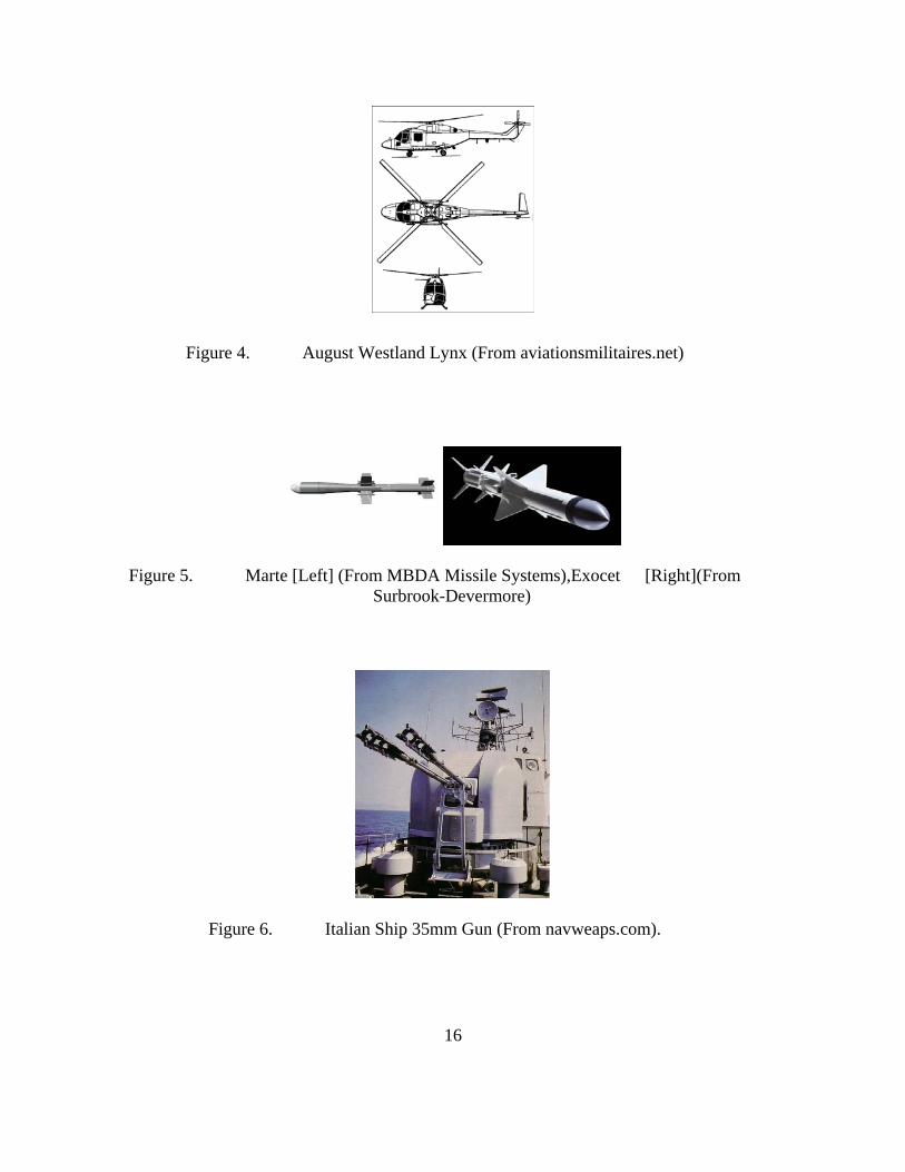
helicopters. We utilized cost data on the Augusta Westland Lynx, as depicted in Figure

4, to estimate the cost of an mid-sized helicopter to be US 31M FY12$ (Jane’s All The

World’s Aircraft, 2011). From the data distribution in Jane’s Fighting Ships, we

determined the average crew complement for OPV’s as a function of the employment of

on-board helicopters and armament configuration. Armament configurations investigated

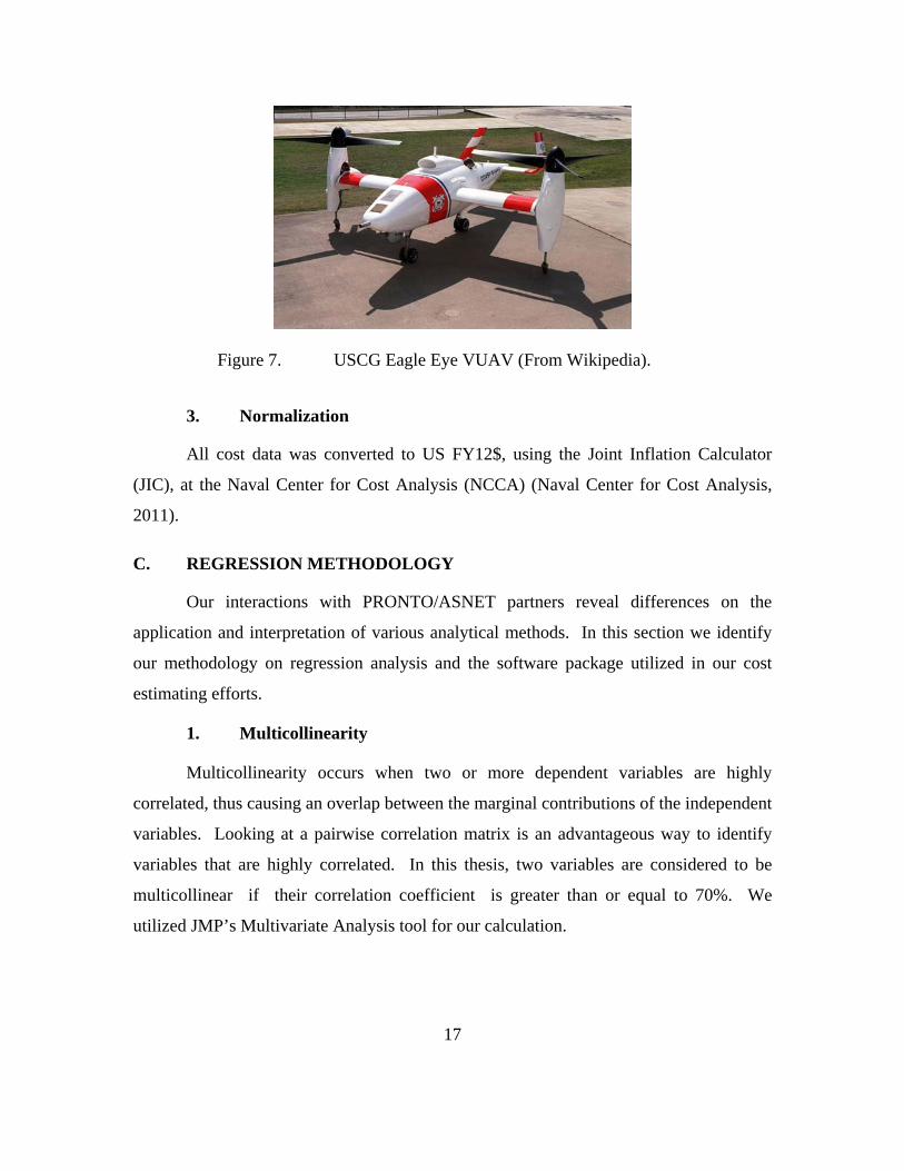
consisted of missiles and a 35mm gun system. Missiles used for both the Italian base

model and this investigation were Exocet and Marte type, images of which are in Figure

5. The cost of an Exocet missile was determined, by analogy to the Harpoon missile, at

US 1.2M FY12$ (U.S. Navy, 2009). The cost and crew complement of a Marte missile

were estimated as half those of the Harpoon’s. Cost data on an Italian 35mm gun

system, depicted in Figure 6, was determined through expert judgment (A. Bonvicini,

personal communication, July 30, 2012). VUAVs were determined to be half the size of

a helicopter based on operational considerations reported on the USCG National Security

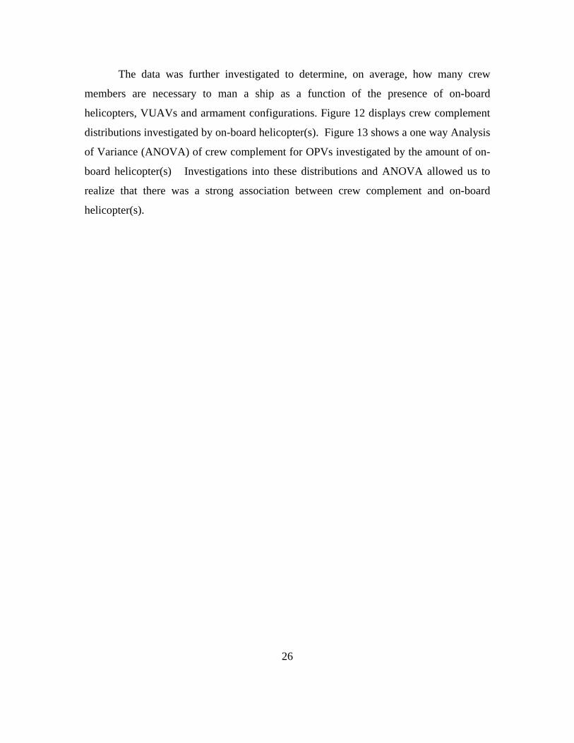
Cutter (Beshears & Peterson, 2004). The cost of a VUAV was determined using cost

data from the USCG’s Eagle Eye VUAV, depicted in Figure 7, with an estimated cost of

US 11.2M FY12$

16

Figure 4. August Westland Lynx (From aviationsmilitaires.net)

Figure 5. Marte [Left] (From MBDA Missile Systems),Exocet [Right](From Surbrook-Devermore)

Figure 6. Italian Ship 35mm Gun (From navweaps.com).

17

Figure 7. USCG Eagle Eye VUAV (From Wikipedia).

3. Normalization

All cost data was converted to US FY12$, using the Joint Inflation Calculator

(JIC), at the Naval Center for Cost Analysis (NCCA) (Naval Center for Cost Analysis,

2011).

C. REGRESSION METHODOLOGY

Our interactions with PRONTO/ASNET partners reveal differences on the

application and interpretation of various analytical methods. In this section we identify

our methodology on regression analysis and the software package utilized in our cost

estimating efforts.

1. Multicollinearity

Multicollinearity occurs when two or more dependent variables are highly

correlated, thus causing an overlap between the marginal contributions of the independent

variables. Looking at a pairwise correlation matrix is an advantageous way to identify

variables that are highly correlated. In this thesis, two variables are considered to be

multicollinear if their correlation coefficient is greater than or equal to 70%. We

utilized JMP’s Multivariate Analysis tool for our calculation.

18

2. Measures of Goodness of Fit and Cost Results

The analysis tools for JMP were utilized to investigate distributions and perform

regressions for this thesis. In utilizing the “fit model” tool in JMP, a stepwise fit was first

investigated with dependent variables inclusive of all response surfaces for model effect

construction. The stepwise option allowed us to achieve the best regression fit by

facilitating a search and selection operation among many model variations. Further

determination of a good fit was confirmed by looking at the Lack of Fit’s p-value of the

F-statistic, the Parameter Estimate dependent variable’s p-value of the t-statistic, and the

Summary of Fit’s and adjusted. Confidence Intervals (CI) for the parameter

estimates were also calculated.

a. Prob > │t│

Assist in determining whether the dependent variable is “useful” in the

model. If less than alpha then we prefer the dependent variable in our model. In JMP,

this is associated with a p-value next to the variables regressed. An asterisk is associated

with acceptable p-values for dependent variables in the fit.

b. Prob > F

Informs whether the overall model is preferred to the mean of the original

dependent variable values. In JMP the F statistic signifies the differences between groups

with respect to their means, the lower the probability that the population means are equal,

the more significant the regression model is.

c. and adjusted

Indicates that potion of Total Variation is accounted for by the regression.

It is also an indicator of our confidence in predicted values. In JMP R is utilized for

model comparison with the same number of regressors while R adjusted is utilized for

model comparisons with a varying number of regressors. Indication that a model has a

better fit is by determining the greatestR .

d. CI

Provides a lower and upper estimate which allows an association of risk

based on the alpha level, thus indicating the reliability of the estimate. In JMP, you can

19

set the alpha level via model specifications right before fitting your model. This will

provide output of the upper and lower parametric equations associated with your desired

confidence level.

20


21

IV. COST ANALYSIS

In this chapter, we provide a detailed description of the production cost estimating

dashboard along with the “under the hood” analysis that was used to build it.

A. PRODUCTION COST ESTIMATION DASHBOARD

1. Development

A dashboard was created that quickly displays the changing OPV production cost

estimate as a function of combat system configuration and mission dependent combat

capabilities. This dashboard is one of several parallel efforts being built by NPS students

for the PRONTO/ASNET NICOP initiative.

The inputs for the dashboard are: maximum speed capability, number of on-

board helicopters, number of on-board VUAVs, number and type of missiles on board

(Marte or Exocet), the inclusion of a 35mm gun system, the presence of a helicopter in

the Area of Operations (AO), and the number of OPVs to be produced. These inputs are

requested through a visual basic pop-up screen when the program is opened. The input

screen of the dashboard is depicted in Figure 8.

The output screen of the dashboard can be viewed in Figure 9. It displays the cost

estimates (in US FY12$M), and 80% CI, for:

First OPV in production ( so-called “T1”)

Average cost of all OPVs produced, and the distribution of this estimate across the single digit SWBSE.

External costs of helicopters, VUAVs, the 35mm gun system, and missiles, as well the total of these items

The learning curve associated with OPV production

The associated overall length, overall beam, full load displacement, average crew complement, light ship weight, and average dollar per pound, for a ship which is the average of current OPVs in operation.

22

Figure 8. Opening, Input, page of the Dashboard

Figure 9. Output page of the Dashboard

23

The dashboard’s purposes are to develop and display production cost estimate,

based on various combat configurations. The dashboard user configures the combat

components through inputs of: the number of OPV’s to be produced, the number of on-

board helicopters and on-board VUAVS, the type and amount of missiles, maximum

speed capability, whether the OPV will use a 35mm gun system, and whether the use of

a helicopter is in the OPV’s AO (The dashboard quickly provides an average ship

production cost estimate with an 80% CI for this cost estimate. This estimate is

developed through a series of steps that produces a flow of information. This flow is

determined by:

Average crew complement, based on aerial assets and weapon configurations.

Maximum speed, which is an input variable for this model.

Length, which is determined by a parametric equation built from maximum speed and crew complement via JMP.

Beam, determined through a parametric equation built from length via JMP.

Full load displacement, determined through a parametric equation built from beam via JMP.

The parametric equation from the regression analysis performed on light ship weight against full load displacement via JMP.

The $34.64 per pound calculation, based on the production of four 270ft WMECs, which was calculated from the NAVSEA 05C data.

Figure 10 displays this flow, called a “Synthesis Flow,” along with associated

parametric equations and associated R values.

24

Figure 10. Synthesis Flow via Distributional and Regression Analysis

B. ANALYZING THE DATA

1. Jane’s Fighting Ships

Jane’s Fighting Ships provided data on 45 OPVs from 28 different nations. This

data represented OPVs that ranged between 109 to 418ft in overall length, 21 to 54ft in

overall beam, 377,000 to 9,211,000lbs of full load displacement (188.5 to 4,605.5 short

tons), 12 to 35kts of maximum speed capabilities, complemented with crews between 6

to 162 sailors, having the capability to hold either 0, 1, or 2 medium sized helicopter(s),

and armament configurations consisting of missiles representative of Exocet or Harpoon

missiles, or missiles similar in dimension and performance, and guns ranging from

7.62mm to 100mm (Jane’s Fight Ships, 2012).

25

The six figures in Figure 11, provide the distribution of the OPV factors from

these 45 data points. For example, looking at the distribution of length we can see that

although the ships represented by the data range from 100 to 450ft, the majority of them

are between 150 and 300 ft. We can see that this distribution holds a Normal 3 Mixture

property, which can indicate normality once the data is separated, as seen in the darker

portion of the graph between 150 to 450ft.

Distributions Length

Normal 3 Mixture

Distributions Beam

Normal 2 Mixture

Distributions Displacement

Normal 3 Mixture

Distributions Max Speed

Normal 3 Mixture

Distributions Crew

Gamma(2.71571,21.48,0

Distributions Helicopter

Figure 11. Distributions of OPV Factors

26

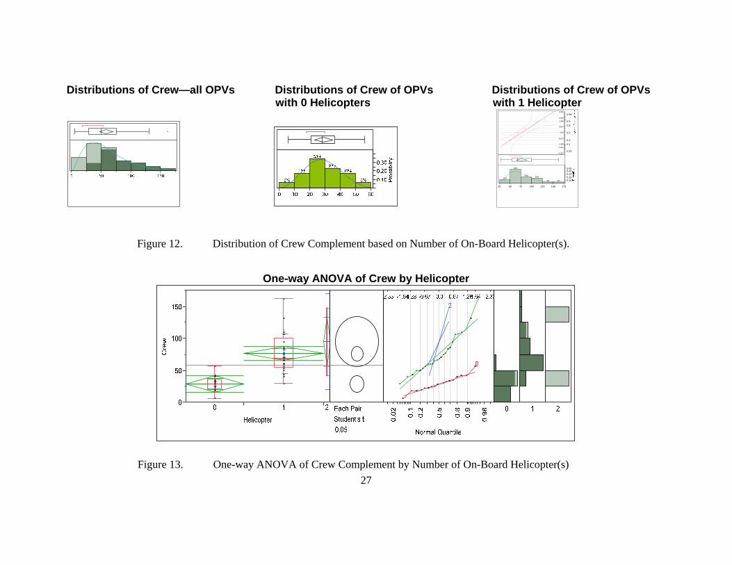
The data was further investigated to determine, on average, how many crew

members are necessary to man a ship as a function of the presence of on-board

helicopters, VUAVs and armament configurations. Figure 12 displays crew complement

distributions investigated by on-board helicopter(s). Figure 13 shows a one way Analysis

of Variance (ANOVA) of crew complement for OPVs investigated by the amount of on-

board helicopter(s) Investigations into these distributions and ANOVA allowed us to

realize that there was a strong association between crew complement and on-board

helicopter(s).

27

Distributions of Crew—all OPVs Distributions of Crew of OPVs Distributions of Crew of OPVs with 0 Helicopters with 1 Helicopter

Figure 12. Distribution of Crew Complement based on Number of On-Board Helicopter(s).

One-way ANOVA of Crew by Helicopter

Figure 13. One-way ANOVA of Crew Complement by Number of On-Board Helicopter(s)

-2.33

-1.64

-1.28

-0.67

0.0

0.67

1.28

1.64

2.33

0.5

0.8

0.9

0.2

0.1

0.02

0.98

12%

44%

20%16%

4% 4% 0.100.200.300.400.50

25 50 75 100 125 150 175

28

2. NAVSEA 05C Production Cost Data on USCG’s 270’ WMEC

We estimated fully burdened labor cost at $66/hr, built up as follows:

A mean rate for ship and boat building of $22/hour from the Bureau of labor Statistics (BLS) plus

A “wrap rate”, to cover overhead, general and administrative cost, profit, and fringe benefits, of 200% (Bureau of Labor Statistics, 2011 & D. Nussbaum, personal communication, February 15, 2012).

We then estimated ship production cost on a dollar per pound basis. We used

$34.64/lb which we developed by considering both the labor cost and material cost per

ship, averaged across the four WMEC ships for which we have data. This dollars-per-

pound estimate is further allocated to the nine SWBS elements, in proportion to weight,

as shown in Figure 14.

Further, we developed a unit-theory learning curve from the four data points, and

we used this learning curve to estimate costs for ships beyond a four-ship class. Figure 15

depicts the learning curve, which has a first unit cost of 111 US FY12$M and a learning

curve slope of 91% .

Figure 14. Distribution of Weight (lbs) based on single digit SWBSE (After NAVSEA 05C)

46%

13%

6%

4%

18%

12% 1%0% 0%

WBS Distribution of weight (lbs)

100 200 300

400 500 600

700 800 900

29

Figure 15. Learning Curve associated with NAVSEA 05C 270 ft WMEC Data (After NAVSEA 05C)

3. Dr. Nussbaum’s OPV Weight Data

Light ship weight data was acquired for three USCG cutters: The 378ft High

Endurance Cutter (WHEC) at 5,412,480lbs, the 270ft WMEC at 2,899,456lbs, and the

210ft WMEC at 1,710,867lbs. We used these three data points to model light ship weight

as a function of full load displacement. The three data points are listed in Table 4, where

deadweight is calculated by subtracting light ship weight from full load displacement.

Table 4. Light Ship Weight Data displayed in JMP Database.

y = 1E+08x-0.131

R² = 0.9915

90

100

110

120

0 1 2 3 4 5

Un

it C

ost

Mill

ion

s

Qty

Learning Curve

Learning Curve

30

C. DISTRIBUTION ANALYSIS

Crew complement was determined for each of four OPV configuration. For each

configuration, we used the mean crew complement of similarly configured OPVs in

Jane’s Fighting Ship. Descriptive data are displayed in Figure 16 and Table 5 displays

means for each configuration The four configurations are:.

An OPV without an on-board helicopter and without a gun system or having guns smaller than 30mm

An OPV without an on-board helicopter with a 30mm gun system or greater

An OPV with an on-board helicopter and gun system less than 25mm

An OPV with an on-board helicopter and a gun system between 25mm and 35mm.

Distribution of Crew Complement Distribution of Crew Complement for ships with 0 helicopters and gun ships with 0 helicopters and gun systems less than 30mm: Mean =27 systems of 30mm or greater: Mean = 36

Distribution of Crew Complement Distribution of Crew Complement for ships with 1 helicopter and gun for ships w/ 1 helicopter and gun Systems less than 25mm: Mean=62 systems between 25mm & 35mm Mean=71

Figure 16. More Detailed Distribution Analysis of Crew Complement

31

Table 5. Average Crew Complement based on 35mm Gun System and 1 On-Board Helicopter.

We are still estimating crew size, this time only for combat factors not mentioned

in the distributional analysis. An OPV with two on-board helicopters was determined by

taking the average of the only two reported OPVs employing two helicopters from the

Jane’s Fighting Ships data, resulting with an average crew complement of 95 people.

VUAV’s were determined by the fact that they were reported to take up nearly half the

operating space via the insight gained on a report of the USCGs National Security Cutter.

Therefore the average crew complement was calculated in associated progression steps,

based upon the on-board helicopter(s) average crew complement. Missiles were

determined from the data of four ships from the Jane’s Fighting Ships data. By removing

the determined crew complements and performing calculations based upon each missile,

a crew complement average was determined to represent each missile with four persons.

The missiles reported in the data were either Exocet or Harpoon, which are both very

similar in size and payload. A crew complement for Marte missiles were determined by

halving the average crew complement estimated for Exocet type missiles, setting average

crew complement down to two persons per Marte missile.

D. REGRESSION ANALYSIS

We used JMP to investigate multicollinearity and to do stepwise regression.

1. Multicollinearity

We checked the data from Jane’s Fighting Ships for multicollinearity, and we

found significant linear relationships among displacement, length and beam, as

32

highlighted in the pairwise correlation matrix provided in Table 6 and graphically

depicted in Figures 17 and 18.

Table 6. Multivariate Correlations of OPV factors.

MultivariateCorrelations Displacement Length Beam Max Speed CrewDisplacement 1.0000 0.9285 0.9134 -0.1349 0.7155Length 0.9285 1.0000 0.9355 0.0425 0.7737Beam 0.9134 0.9355 1.0000 -0.1449 0.6509Max Speed -0.1349 0.0425 -0.1449 1.0000 0.1028Crew 0.7155 0.7737 0.6509 0.1028 1.0000

Scatterplot Matrix

Figure 17. Graphical Representation of the Correlation between OPV factors.

33

Ellipsoid 3D

Figure 18. 3D Plot Showing Strong Multicollinearity between OPV Factors: Length, Beam and Displacement

2. Overall Length

We modeled length, using a stepwise fit, against crew complement and speed.

The output to the regression analysis is in Table 7, with the highlighted items confirming

significance in the model and the model parameters. Further interactions between overall

length against crew complement and maximum speed capability allows for further

investigation on how length is determined. In Figure 20, you can see that length has a

saddle-point in its graphical representation of the factors interacting with crew

complement and maximum speed. This observation allows us to recognize that adding

on-board helicopter may add to cost.

34

Table 7. JMP Regression Output for Overall Length.

Summary of Fit RSquare 0.802056RSquare Adj 0.770801Root Mean Square Error 16718.72Mean of Response 61482.21Observations (or Sum Wgts) 45

Analysis of Variance Source DF Sum of Squares Mean Square F Ratio Model 6 4.3038e+10 7.173e+9 25.6622 Error 38 1.0622e+10 279515651 Prob > F C. Total 44 5.366e+10 <.0001*

Parameter Estimates Term Estimate Std Error t Ratio Prob>|t| Lower 95% Upper 95%

Intercept 5869.5891 15085.64 0.39 0.6994 -24669.69 36408.873

Max Speed 2165.3316 602.9703 3.59 0.0009* 944.68194 3385.9812

Crew 387.05542 133.3916 2.90 0.0061* 117.01816 657.09267

(Max Speed-22.2222)*(Max Speed-22.2222) -221.7492 71.91482 -3.08 0.0038* -367.3331 -76.16524

(Max Speed-22.2222)*(Crew-58.3333) 62.442609 19.13465 3.26 0.0023* 23.706538 101.17868

(Crew-58.3333)*(Crew-58.3333) -11.41778 3.231594 -3.53 0.0011* -17.9598 -4.875764

(Crew-58.3333)*(Crew-58.3333)*(Crew-58.3333) 0.115227 0.042296 2.72 0.0097* 0.0296035 0.2008505

Prediction Expression

35

Interaction Profiles

Figure 19. Interaction Profiles for Overall Length

Figure 20. 3D Plot for Overall Length, Crew Complement & Maximum Speed

100

200

300

400

100

200

300

400

Max Speed

6

162

12

35

Crew

36

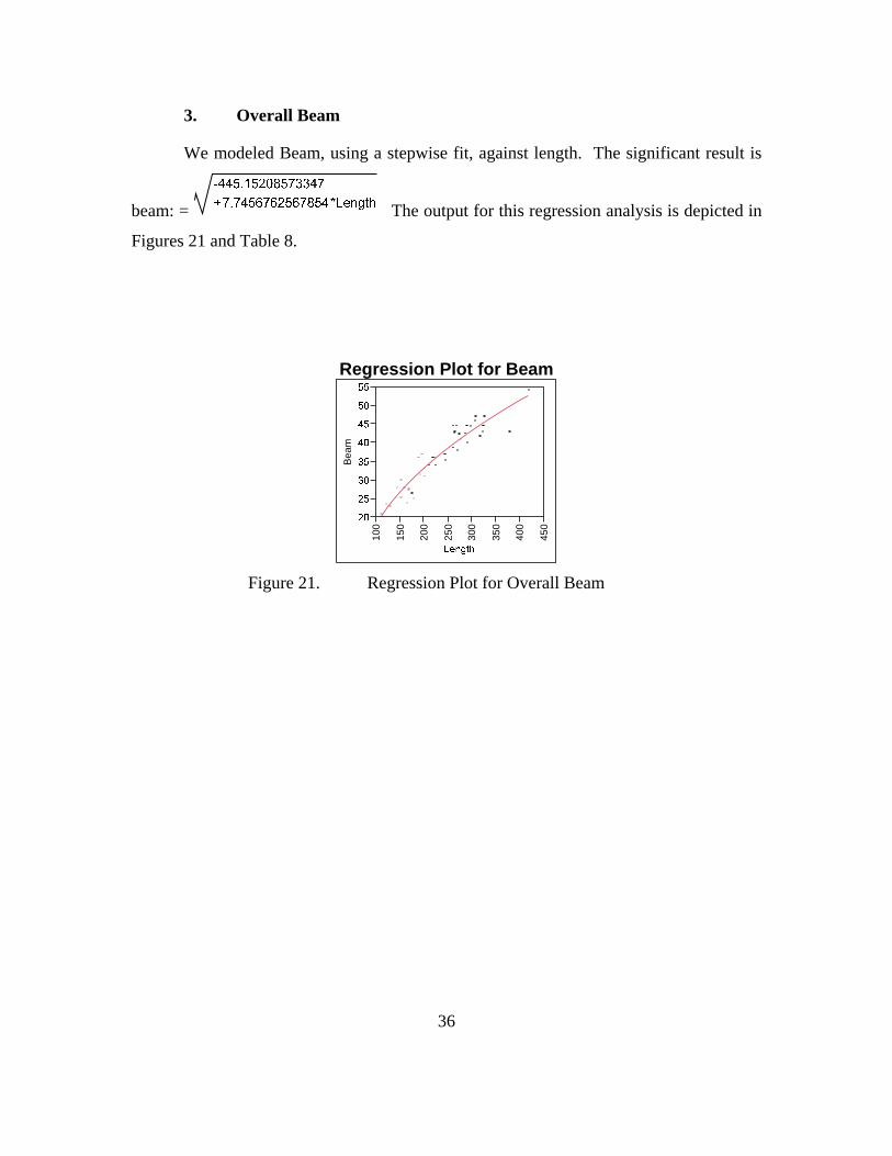
3. Overall Beam

We modeled Beam, using a stepwise fit, against length. The significant result is

beam: = The output for this regression analysis is depicted in

Figures 21 and Table 8.

Regression Plot for Beam

Figure 21. Regression Plot for Overall Beam

Bea

m

100

150

200

250

300

350

400

450

37

Table 8. JMP Regression Output for Overall Beam.

Summary of Fit

RSquare 0.879699 RSquare Adj 0.876901

Root Mean Square Error 203.0922 Mean of Response 1398.878

Observations (or Sum Wgts) 45

Analysis of Variance

Source DF Sum of Squares Mean Square F RatioModel 1 12969365 12969365 314.4359 Error 43 1773597 41246.451 Prob > F

C. Total 44 14742962 <.0001*

Parameter Estimates

Term Estimate Std Error t Ratio Prob>|t| Lower 95% Upper 95%Intercept -445.1521 108.3099 -4.11 0.0002* -663.5798 -226.7244 Length 7.7456763 0.436811 17.73 <.0001* 6.8647635 8.626589


38

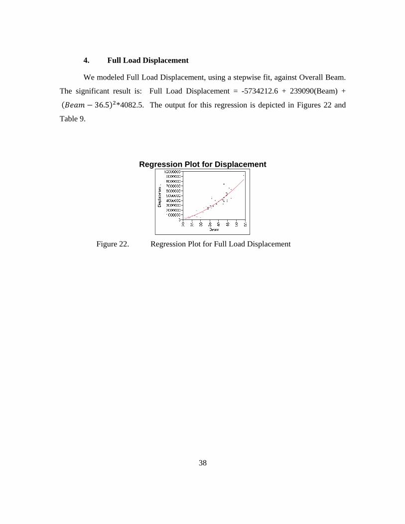
4. Full Load Displacement

We modeled Full Load Displacement, using a stepwise fit, against Overall Beam.

The significant result is: Full Load Displacement = -5734212.6 + 239090(Beam) +

36.5 *4082.5. The output for this regression is depicted in Figures 22 and

Table 9.

Regression Plot for Displacement

Figure 22. Regression Plot for Full Load Displacement

39

Table 9. JMP Regression Output for Full Load Displacement.

Summary of Fit

RSquare 0.851564RSquare Adj 0.844495Root Mean Square Error 807517.2Mean of Response 3261942Observations (or Sum Wgts) 45

Analysis of Variance Source DF Sum of Squares Mean Square F RatioModel 2 1.5712e+14 7.856e+13 120.4748Error 42 2.7388e+13 6.521e+11 Prob > FC. Total 44 1.8451e+14 <.0001*

Parameter Estimates Term Estimate Std Error t Ratio Prob>|t| Lower 95% Upper 95%

Intercept -5734213 610080.2 -9.40 <.0001* -6965404 -4503021

Beam 239090.06 15427.29 15.50 <.0001* 207956.52 270223.6

(Beam-36.5447)*(Beam-36.5447) 4082.4689 1848.588 2.21 0.0327* 351.86726 7813.0705


40

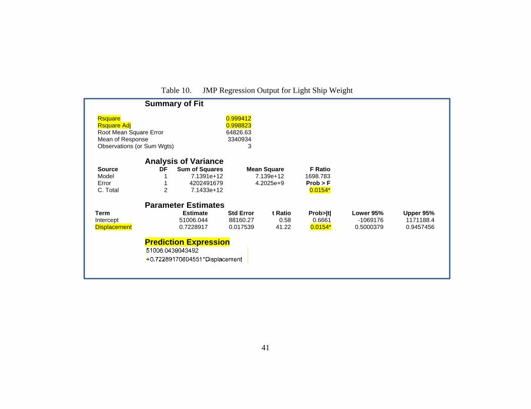
5. Light Ship Weight

We modeled light ship weight, using a stepwise fit, against full load displacement.

The significant result is light ship weight = 51006 + .72(Displacement)

Since the majority of the weight data acquired was reported in full load

displacement, and since we had already confirmed, through our analysis, that light ship

weight and full load displacement are related, we utilized data points that contained both

light ship weight and full load displacement and refreddion analysis to model that

relationship. In that way we are able to derive light ship weight from the remaining data

points that only report full load displacement.

The use of OPVs within a limited range and acquired data is mostly attributed to

full load displacement rather than light ship weight. It is necessary to use this estimate to

build more light ship weight data points that can strongly represent the variability of

OPVs currently in operation. The outputs for this regression analysis is depicted in

Figures 23 and Table 10.

An analysis to determine light ship weight was completed on the three points

containing both light ship weight and full load displacement and it was evident that

although the amount of data was small, light ship weight showed significant relation to

full load displacement.

Regression Plot for Weight against Displacement

Figure 23. Regression Plot for Weight against Displacement

41

Table 10. JMP Regression Output for Light Ship Weight

Summary of Fit Rsquare 0.999412Rsquare Adj 0.998823Root Mean Square Error 64826.63Mean of Response 3340934Observations (or Sum Wgts) 3

Analysis of Variance Source DF Sum of Squares Mean Square F RatioModel 1 7.1391e+12 7.139e+12 1698.783Error 1 4202491679 4.2025e+9 Prob > FC. Total 2 7.1433e+12 0.0154*

Parameter Estimates Term Estimate Std Error t Ratio Prob>|t| Lower 95% Upper 95%Intercept 51006.044 88160.27 0.58 0.6661 -1069176 1171188.4Displacement 0.7228917 0.017539 41.22 0.0154* 0.5000379 0.9457456


42

E. UTILIZATION OF THE DASHBOARD

A goal of this thesis is to develop a dashboard that quickly displays the changing

OPV production cost estimate as a function of combat system configuration and mission

dependent combat capabilities. The production cost estimates derived through the use

of the cost estimating tool developed for this thesis and for the NPS efforts towards the

ASNET/PRONTO simulation analysis that guided the combat system configurations,

provided an opportunity to validate the developed cost model by comparing various costs

estimates based on these different combat configurations. These cost estimates proved to

be a good determinant for future decision making considerations.

The cost model developed for this thesis effort, paired with individual simulation

outputs that others at NPS developed in support of ASNET/PRONTO, permit

simultaneous linkages across combat system configuration, combat effectiveness and cost

estimates. We used the cost estimating model that we developed, and the dashboard

within which it is embedded to demonstrate our ability to develop production cost

estimates from simulation outputs

In this section we demonstrate the dashboard’s costing ability in relation to the

simulation outputs done by Royal Thai Navy CDR Peerapong Yoosiri, LT Jason

McKeown, and LT Joseph Ashpari. This detailed investigation gives insight into the

dashboards utilization abilities.

1. Royal Thai Navy CDR Peerapong’s MIO Simulation

CDR Yoosiri Peerapong of the Royal Thai Navy developed a simulation model,

complemented with an advanced design of experiments (DOE) approach. His model

replicated the simulation efforts from the Italian model’s MIO mission and improved

upon the research to investigate significant input parameters. These pinpointed more

realistic combat attributes that more accurately defined the mission effectiveness. In an

effort to explore relationships from his simulation, the utilization of partition platforms in

JMP were used to recursively partition the simulation output data in order to investigate

relationships. Through this method, the following was determined:

43

The Italian model representing the MIO mission indicated that the MOE was

substantially higher when operating in a small area, and within these small areas, using an

OPV with an on-board helicopter increased the MOE. With identification of a 35 to 40

NM area, the MOE increased from 73.4, for an OPV with no on-board helicopter, to 88.6,

for an OPV with one on-board helicopter. Considering an OPV that has a max speed of

22kts, the maximum speed considered in both simulation efforts, and that is not

complemented with a helicopter would cost on average between 54.35M and 79.61M;

whereas an OPV that has a maximum speed of 22kts and is complemented with a

helicopter would cost, on average, between 94.38M and 127.93M. Therefore based on

the conclusions of the Italian model, a decision maker would have to decide whether

spending an extra 40M to 50M per ship would be worth the greater MOE for this

mission. All aspects of the ships composed in this analysis via the dashboard are depicted

in Table 11, specifically labeled scenario a.

CDR Peerapong’s simulation that was used to replicate the Italians’ also

concluded that in a smaller area an OPV complemented with a helicopter on-board would

significantly increase the MOE. His model went a step further by identifying not only a

smaller area, but a medium and a larger area. This simulation analysis concluded that

hands-down complementing an OPV with an on-board helicopter would increase the

MOE of the MIO mission despite the area. It is important to understand the MOE

employed by CDR Peerapong’s model and the Italian model are both represented on

different scales. They share the ability to evaluate for both positive and negative

variations; however, they are representative of a similar baseline approach.

In a substantial small area, smaller than the one analyzed in the Italian based

model, an MOE goes from 38.8 to 61.2 by including an on-board helicopter. Considering

a similar area as mentioned for the Italian model, the MOE goes from 23.3 to 43.5 by

including the on-board helicopter and goes from 17.3 to 31.2, respectively, for a really

large area.

CDR Peerapong further advanced his simulation to distinguish between using a

parallel searching pattern versus a random searching pattern.

44

He concluded that the significance lied within the size of the area searched when

utilizing the parallel searching method; this was complemented by the maximum speed

ability of the OPV. For instance in a substantial large area where the proposed armed

smuggling boat, represented as a red agent in the MANA simulation as seen in Figure 24,

has the max speed capability greater than 26.3kts, an OPV with a max speed less than

33.7kts only has an MOE of 24% whereas an OPV with a max speed above 33.7kts has a

MOE of 35%. In order to use these factors to investigate the cost model created for this

thesis, the average cost of a ship that has a max speed of 33kts is between 21.78M to

41.37M while a ship that has a max speed of 34kts is between 13.09M to 31.53M. This is

explained by the fact that the cost model developed utilizes an average of the propulsion

systems based off the 48 ships represented in Jane’s Fighting Ships. If max speed is the

only issue, then accomplishing the combat effectiveness would simply mean building a

smaller ship while utilizing the same engine. This can be seen in Table 11, section b.

In investigating the simulation model using the random search pattern, the

analysis showed that the factor of whether to use an OPV with an on-board helicopter

was the significant implication from the resulting data. For instance, an OPV that did not

have an on-board helicopter had an MOE of 29%, while an OPV with an on-board

helicopter had a MOE of 52%. To place this investigation into a deeper perspective, the

analysis showed that an OPV without an on-board helicopter and having the capability of

a max speed less than 32.9kts that was trying to interdict a red agent that had a max speed

greater than 25kts, resulted in a MOE of 17%, while a non-helicopter OPV that had the

max speed capability above 32.9kts has an MOE of 32%. In cost estimation perspectives,

a non-helicopter OPV that has a max speed of 32kts would have an average cost based

between 28.33M to 49.09M while a non-helicopter OPV that has a max speed capability

of 33kts would have an average cost between 21.78M to 41.37M. Once more we have

the opportunity to show that having a greater maximum speed relies on a smaller ship

with the same engine, thus being more cost effective while increasing the MOE of the

MIO mission from this simulation effort. This can be seen in Table 11, section c.

Although a deeper investigation into the cost model will show that by increasing the

45

maximum speed capabilities once you add various combinations of armament and on-

board flight capabilities, the rate of the cost decrease goes dramatically down, perhaps

reflecting the saddle point represented in Figure 20.

CDR Peerapong further advanced his MIO simulation to include the use of an on-

bard VUAV. The cost model was designed with the capability for OPV architectural

parameter changes based on including up to four VUAVs on-board. The analysis of

CDR Peerapong’s advanced MIO simulation showed there would be a significant MOE

increase when an OPV has an on-board helicopter and is utilizing a VUAV in a very

large area. This analysis was further pinpointed to represent operations where the “red

target” could not achieve a maximum speed over 36.3kts. Within this design and these

constraints a 1-helicopter OPV that had the capability to travel 22kts without the

additional VUAV performed with a 43% MOE while the same OPV that had the

advantage of the additional on-board VUAV performed with a 67% MOE. A 1-

helicopter OPV with a max speed of 22kts w/o an on-board VUAV costs between

85.23M to 115.53M with an external cost of 31M for the helicopter while the same OPV

with the advantage of the on-board VUAV would range from 87.83M to 118.63M with

the external cost of 42.2M for the VUAV and Helicopter. This can be seen below in

Table 11, section d

Table 11. Cost Estimates for MIO Simulation Output Analysis

46

Figure 24. Royal Thai Navy CDR Peerapong’s MANA Simulation—depicting a screenshot of the end-state of a scenario model (Y. Peerapong, Thesis pending

publishing, June 2012).

2. LT Joe Ashpari of the United States Navy

LT Joe Ashpari developed a SAR model that investigated combinations involving

the use of a ships maximum speed capability, the employment of on-board medium sized

helicopters, and the use of on-board VUAVs. Other noise factors represented in LT

Ashpari’s model included: ship search speed, wind speed, datum uncertainty, initial

distance of ship to target, type of search target, environmental control factors, wind

direction, maximum VUAV speed, maximum helicopter speed, VUAV search speed, and

helicopter search speed. This model utilized a DOE method that allowed for the

investigation of responses based on the interconnection over a wide range of values.

Moreover he was able to compile an analysis that determined the best configuration

based on a MOE that defined the time required to identify the given target. His

conclusion showed that in order to identify the target in an average time of 2.74 hours, an

OPV would require no on-board helicopters and 2 on-board VUAVs along with a

capability to travel greater than 8 knots.

With the utilization of the production cost dashboard, it was determined that such

an OPV would have an average cost between 37.77M and 60.22M with an average

external cost of 22.4 million dollars for the VUAVs. Further consideration would

recognize that since the MOE only represents the time to detection and does not represent

travel time to rescue the target, there might be a need to increase the maximum speed

47

capability of the OPV. The initial cost estimation was done in consideration of achieving

an estimate of an OPV with 2 VUAVs and a maximum speed capability greater than 8kts.

Through means of the utilizing the cost model it was determined that the lowest possible

maximum speed for an OPV capable of deploying 2 on-board VUAVs was 13kts.

Increasing this speed would likewise increase the production cost estimation. For

example a 2-VUAV OPV with a maximum speed capability of 20kts, which would be a

more realistic speed capability, is estimated to have an average cost between 79.10M and

108.45M. Figure 25 depicts this analysis with a line graph showing the growth of

architectural design factors and cost estimations as the maximum speed capability of the

ship increases.

LT Ashpari further concluded more ships with a growing mean time to detection.

Thus utilizing the OPV as a platform to launch and retrieve VUAVs and without using

speed as a factor would not require extreme costs based on the cost analysis of the

historical comparisons. Given the understanding that a VUAV is not able to retrieve a

person in a SAR situation, yet a helicopter is would be another factor to be further

analyzed by decision makers. A decision maker can utilize the cost estimates to decide

whether it is more appealing to design an OPV capable of detecting a SAR target really

quickly and has maximum speed capabilities to sail to its target or whether it is more

beneficial to design an OPV capable of deploying a helicopter and VUAV for a higher

cost, yet having the ability to interact with a SAR target in a more efficient timely

manner. Table 12 shows the cost comparisons based on LT Ashpari’s model.

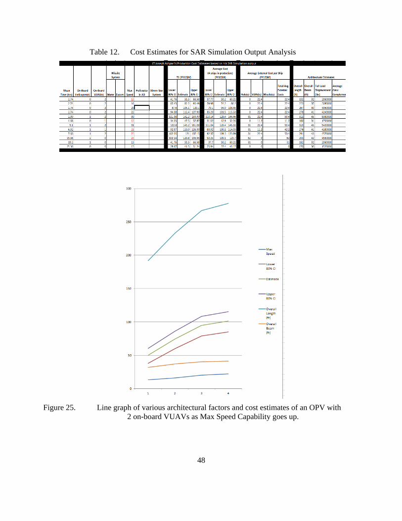
48

Table 12. Cost Estimates for SAR Simulation Output Analysis

Figure 25. Line graph of various architectural factors and cost estimates of an OPV with 2 on-board VUAVs as Max Speed Capability goes up.

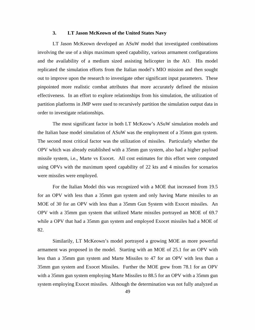
49

3. LT Jason McKeown of the United States Navy

LT Jason McKeown developed an ASuW model that investigated combinations

involving the use of a ships maximum speed capability, various armament configurations

and the availability of a medium sized assisting helicopter in the AO. His model

replicated the simulation efforts from the Italian model’s MIO mission and then sought

out to improve upon the research to investigate other significant input parameters. These

pinpointed more realistic combat attributes that more accurately defined the mission

effectiveness. In an effort to explore relationships from his simulation, the utilization of

partition platforms in JMP were used to recursively partition the simulation output data in

order to investigate relationships.

The most significant factor in both LT McKeow’s ASuW simulation models and

the Italian base model simulation of ASuW was the employment of a 35mm gun system.

The second most critical factor was the utilization of missiles. Particularly whether the

OPV which was already established with a 35mm gun system, also had a higher payload

missile system, i.e., Marte vs Exocet. All cost estimates for this effort were computed

using OPVs with the maximum speed capability of 22 kts and 4 missiles for scenarios

were missiles were employed.

For the Italian Model this was recognized with a MOE that increased from 19.5

for an OPV with less than a 35mm gun system and only having Marte missiles to an

MOE of 30 for an OPV with less than a 35mm Gun System with Exocet missiles. An

OPV with a 35mm gun system that utilized Marte missiles portrayed an MOE of 69.7

while a OPV that had a 35mm gun system and employed Exocet missiles had a MOE of

82.

Similarily, LT McKeown’s model portrayed a growing MOE as more powerful

armament was proposed in the model. Starting with an MOE of 25.1 for an OPV with

less than a 35mm gun system and Marte Missiles to 47 for an OPV with less than a

35mm gun system and Exocet Missiles. Further the MOE grew from 78.1 for an OPV

with a 35mm gun system employing Marte Missiles to 88.5 for an OPV with a 35mm gun

system employing Exocet missiles. Although the determination was not fully analyzed as

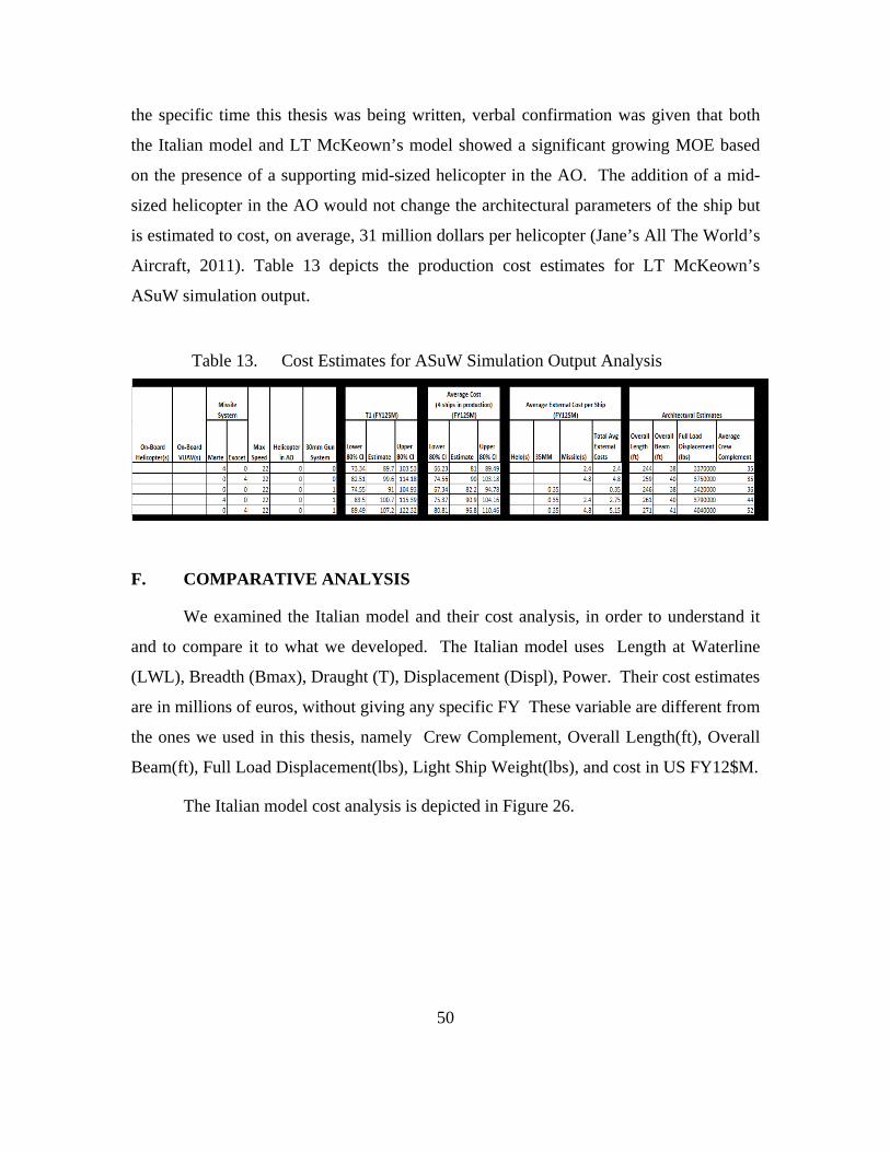
50

the specific time this thesis was being written, verbal confirmation was given that both

the Italian model and LT McKeown’s model showed a significant growing MOE based

on the presence of a supporting mid-sized helicopter in the AO. The addition of a mid-

sized helicopter in the AO would not change the architectural parameters of the ship but

is estimated to cost, on average, 31 million dollars per helicopter (Jane’s All The World’s

Aircraft, 2011). Table 13 depicts the production cost estimates for LT McKeown’s

ASuW simulation output.

Table 13. Cost Estimates for ASuW Simulation Output Analysis

F. COMPARATIVE ANALYSIS

We examined the Italian model and their cost analysis, in order to understand it

and to compare it to what we developed. The Italian model uses Length at Waterline

(LWL), Breadth (Bmax), Draught (T), Displacement (Displ), Power. Their cost estimates

are in millions of euros, without giving any specific FY These variable are different from

the ones we used in this thesis, namely Crew Complement, Overall Length(ft), Overall

Beam(ft), Full Load Displacement(lbs), Light Ship Weight(lbs), and cost in US FY12$M.

The Italian model cost analysis is depicted in Figure 26.

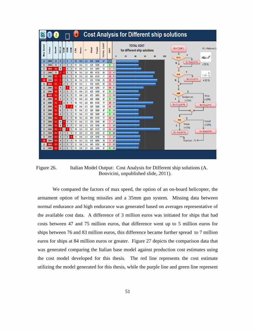
51

Figure 26. Italian Model Output: Cost Analysis for Different ship solutions (A. Bonvicini, unpublished slide, 2011).

We compared the factors of max speed, the option of an on-board helicopter, the

armament option of having missiles and a 35mm gun system. Missing data between

normal endurance and high endurance was generated based on averages representative of

the available cost data. A difference of 3 million euros was initiated for ships that had

costs between 47 and 75 million euros, that difference went up to 5 million euros for

ships between 76 and 83 million euros, this difference became further spread to 7 million

euros for ships at 84 million euros or greater. Figure 27 depicts the comparison data that

was generated comparing the Italian base model against production cost estimates using

the cost model developed for this thesis. The red line represents the cost estimate

utilizing the model generated for this thesis, while the purple line and green line represent

52

the upper and lower 80% CI, respectively. The light blue line represents the Italian

model cost estimates that are composed of ships with higher power components, while

the dark blue line represents the ships with lower power components.

Figure 27. Comparison Graph representing US Cost model against Italian Cost model.

53

V. SUMMARY AND CONCLUSION

In this chapter we summarize the use of the cost model as it applies to the NICOP

initiative. We also describe the framework and how to apply it to future MBSE designs.

Finally, we provide ideas for improvements to the cost estimating model and possibilities

for future work.

A. UTILIZATION IN NICOP INITIATIVE

The cost model supports the NICOP initiative by providing cost estimates of ship

designs that come from the simulation models. These cost estimates allowed for further

investigation of MBSE designs within the tradespace of the MBSE paradigm.

B. THE COST MODEL FRAMEWORK

We have succeeded in developing cost estimates which are responsive to combat

design and naval architecture considerations.

1. How to Apply this to Future MBSE Designs

The work done in this thesis can be applied to future MBSE designs. The steps

necessary to do this are:

Collect data that are from systems that are analogous to the system being investigated.

Identify links between operational factors and architectural parameters via regression analysis.

This process, outlining the steps to achieve this framework, is depicted in Figure 28. The steps to achieve this include:

Identify the factors that define the operational requirements of the system

Identify the factors that affect the architectural engineering of the system

Identify systems analogous to what you are developing

Discover the links from cost to architectural design parameters

54

Utilize Regression Analysis, Analogy, and Expert Judgment to determine these links.

Link architectural design parameters to operational requirement factors

Utilizing Regression Analysis as well as other analysis methods that best represent the flow from one attribute to the other.

55

Figure 28. Depiction of the process flow in developing a MBSE production cost model that changes reflective to changes in combat configurations. (Images from (left to right): navweaps.com, surbrook.devermore.net, mnvdet.com, en.wikipedia.org,

military-pilots.blogspot.com, 123rf.com, & all-silhouettes.com).

56

C. IMPROVEMENTS FOR BETTER ANALYSIS

Research projects necessarily have time constraints, data constraints, and

associated design constraints, all of which impacted this thesis. Areas for future

improvement and research include:

1. Propulsion Systems

The investigation into the design components surrounding the propulsion systems

was not applied in this study, based on time constraints. The ability to place further

emphasis on propulsion attributes would allow for a more precise cost estimate.

2. Hull Material

Investigating the fabrication of the metal used to construct the ship would provide

insight into developing a more comprehensive cost estimating model.p.

3. Complexity Models

Ship hull complexity designs were not used in the development of this model.

There exist various hulls that stray from the simple single hull construction as well as

attributes within the single hull construction that give a deeper understanding into the

complexity of the engineering design. This could be applied to a more comprehensive

cost model.

D. USING THIS MODEL FOR NEXT SHIP–BIGGER SHIP–POSSIBLY LSDX

We believe this model and its framework could easily be adapted for a bigger ship

or even a different system altogether. We would like to place emphasis on the above

mentioned recommendations to make this cost estimating process more comprehensive.

However, the concept will remain the same. Acquirement of cost data and other LSD

data would allow the design to flourish. Identification of the factors that best represent

the architectural parameters via regression or distribution analysis would allow for further

investigation into a synthesis flow that best represents the design of the ship. Applying

57

cost to this flow via a dollar per pound or other justifiably associated means would allow

for a changing cost estimation representative of the design components of the system as a

whole.

58


59

LIST OF REFERENCES

Arena, M. V. (2006). Why has the cost of Navy ships risen?: A macroscopic examination of the trends in U.S. Naval ship costs over the past several decades. Santa Monica, CA: Rand. Retrieved from http://www.rand.org/pubs/monographs/MG484/

Ashpari, M., & Naval Postgraduate School. (2012). A capability-based approach to analyzing the effectiveness and robustness of an offshore patrol vessel in a search and rescue mission. Naval Postgraduate School. Pending Publication.

Aviationsmilitaires. Retrieved from http://www.aviationsmilitaires.net/display/aircraft/172

Beshears, T., & Peterson, G. I. (2004). The HV-911 Eagle Eye Tiltrotor VUAV: An exciting future for Coast Guard Aviation. American Society of Naval Engineers “ASNE Days” Technical Papers.

Bureau of Labor Statistics. (2011, May). May 2011 National industry-specific occupational employment and wage estimates: NACCS336600—Ship and Boat roBuilding. Retrieved from http://www.bls.gov/oes/current/naics4_336600.htm

Brown, A.J., & Salcedo, J. (2003). Multiple-objective optimization in Naval ship design. Naval Engineers Journal, 115(4), 49-61.

Cadova, L., Kovich, C., & Sargusingh, M. (2012, January 9). An MBSE approach to space suit development. Retrieved from http://nix.nasa.gov/search.jsp?R=20120000721&qs=N%3D4294950110%2B4294944242

Estefan, J. A.(2008). Survey of model-based system engineering (MBSE) methodologies. INCOSE MBSE Initiative. May 23, 2008. Retrieved from http://www.omgsysml.org/MBSE_Methodology_Survey_RevB.pdf

Fischer, J.O., & Holbach, G. (2011). Cost management in shipbuilding: Planning, analysing and controlling product cost in the maritime industry. Koeln, Germany: GKP Publishing.

Hockberger, W. A. (1996). Total system ship design in a supersystem framework. Naval Engineers Journal, 108(3), 147-166.

International Council on System Engineering (INCOSE). (2007, June 24). Incose model based system engineering (MBSE) initiative. Retrieved from http://www.incose.org/enchantment/docs/07docs/07jul_4mbseroadmap.pdf

60

Jane’s All The World’s Aircraft. (2011, Mar 7). Retrived from http://www4.janes.com

Jane’s Fighting Ships (2012). Retrieved from http://www4.jane.com

Kleijnen, J. P. C., Sanchez, S. M., Lucas, T. W., & Cioppa, T. M. (2005). A user's guide to the brave new world of designing simulation experiments. Informs Journal on Computing, 17(3), 263-289. doi:10.1287/ijoc.1050.0136

MBDA Missile Systems. Marte MK2/S. Retrieved from http://www.mbda-systems.com/e-catalogue/#/solutions/maritime/45

McKeown, J., & Naval Postgraduate School. (2012). Analyzing the surface warfare operational effectiveness of an offshore patrol vessel using agent based modeling.. Naval Postgraduate School. Pending Publication

Metric Conversions. Retrieved from http://www.metric-conversions.org/weight/pounds-to-short-tons.htm

Miroyannis, A., & Massachusetts Institute of Technology. Dept. of Mechanical Engineering. (2006). Estimation of ship construction costs. Retrieved from http://dspace.mit.edu/handle/1721.1/36275

Naval Center for Cost Analysis. (2010, January). Joint inflation calculator (JIC). Retrieved from http://www.ncca.mil/services/inflation.cfm

Naval Sea Systems Command Cost Engineering and Industrial Analysis Division. (2008). Ship Cost Estimating Methods. Reproduced for NPS Course 4702.

Navweaps. 35 mm/90 KDC gun in Oerlikon GDM-A Twin Mounting. Retrieved from http://www.navweaps.com/Weapons/WNIT_35mm-90_KDC.htm

Piaszczyk, C. (2011). Model based systems engineering with Department of Defense architectural framework. Systems Engineering, 14(3), 305-326. doi:10.1002/sys.20180

Schneekluth, H., Knovel, & Bertram, V. (1998). Ship design for efficiency and economy (2nd ed.). Oxford ; Boston: Butterworth-Heinemann. Retrieved from http://libproxy.nps.edu/login?url=http://www.knovel.com/knovel2/Toc.jsp?BookID=1683

Surbrook-Devermore. Military Air Vehicles: Exocet Missile. Retrieved from http://surbrook.devermore.net/adaptationsvehicles/militaryair/postwar/other/exocet.html

61

Tepper, N. A., & Massachusetts Institute of Technology. (2010). Exploring the use of model-based systems engineering (MBSE) to develop systems architectures in naval ship design. Cambridge: Massachusetts Institute of Technology. Retrieved from http://edocs.nps.edu/AR/topic/theses/2010/10_Tepper.pdf; http://handle.dtic.mil/100.2/ADA541194

Tupper, E. C., & Muckle, W. (1996). Introduction to naval architecture (3rd ed.). Oxford ; Boston: Butterworth-Heinemann.

The University of Arizona. (2004, December 30). System movement: Autobiographical retrospectives: Contributions to the mathematical foundations of system science and systems engineering. Retrieved from http://www.sie.arizona.edu/sysengr/wymore/WWAutobiography.htm

U.S. Government Accountability Office (GAO). (2007). GAO-07-874, Coast Guard: Challenges affecting deepwater asset deployment and management and effort to address them. Retrieved from http://www.gao.gov/htext/d07874.html

U.S. Navy. (2009). US Navy fact file: Harpoon missile. Retrieved from http://www.navy.mil/navydata/fact_display.asp?cid=2200&tid=200&ct=2

Wikipedia. Bell Eagle Eye. Retrieved from http://en.wikipedia.org/wiki/Bell_Eagle_Eye

Yoosiri, P., & Naval Postgraduate School. (2012). Analyzing offshore patrol vessel capabilities utilizing model-based system engineering. Naval Postgraduate School. Pending Publication.

62


63

INITIAL DISTRIBUTION LIST

1. Defense Technical Information Center Ft. Belvoir, Virginia 2. Dudley Knox Library Naval Postgraduate School Monterey, California

naval postgraduate school will achieve a warship design that effectively links the combat system and...

Documents