navier-stokes equation and applicationnavier-stokes equation and application zeqian chen abstract....
TRANSCRIPT

AN INFINITE LINEAR HIERARCHY FOR THE INCOMPRESSIBLE
NAVIER-STOKES EQUATION AND APPLICATION
ZEQIAN CHEN
Abstract. This paper introduces an infinite linear hierarchy for the homogeneous, incompressiblethree-dimensional Navier-Stokes equation. The Cauchy problem of the hierarchy with a factorized
divergence-free initial datum is shown to be equivalent to that of the incompressible Navier-Stokesequation in H1. This allows us to present an explicit formula for solutions to the incompressible
Navier-Stokes equation under consideration. The obtained formula is an expansion in terms of
binary trees encoding the collision histories of the “particles” in a concise form. Precisely, each termin the summation of n “particles” collision is expressed by a n-parameter singular integral operator
with an explicit kernel in Fourier space, describing a kind of processes of two-body interaction of n
“particles”. Therefore, this formula is a physical expression for the solutions of the incompressibleNavier-Stokes equation.
Contents
1. Introduction 12. Function spaces 53. The Navier-Stokes hierarchy 63.1. Interaction operator 63.2. Definition of solution 74. Uniqueness and equivalence for the Navier-Stokes hierarchy 105. Graphic expression for interaction operators 126. Graphic representation for the Navier-Stokes hierarchy 167. A prior space-time estimates 217.1. Space-time estimates for collision operators 217.2. Space-time estimates for error operators 257.3. Proof for uniqueness 288. A solution formula for the incompressible Navier-Stokes equation 299. Appendix 389.1. Binary trees with marked edges 389.2. Preliminary estimates 40References 42
1. Introduction
We are concerned with the homogeneous, incompressible Navier-Stokes equation in R3
(1.1)
{∂tu+ (u · 5)u = 4u−5p,5 ·u = 0,
with the initial data u(0) = u0 satisfying 5 · u0 = 0. Recall that u = u(t, x) ∈ R3 is the velocity ofthe fluid at position x ∈ R3 and time t > 0, and p = p(t, x) is a scalar field called the pressure of thefluid, while u0 = u0(x) ∈ R3, x ∈ R3, is a given initial velocity vector. By eliminating the pressure p,
Key words: Navier-Stokes equation, Navier-Stokes hierarchy, Cauchy problem, binary tree, solution formula.
1
arX
iv:1
610.
0177
1v3
[m
ath-
ph]
23
Jan
2017
2 Zeqian Chen
the equation (1.1) is reformulated as
(1.2)
{∂tu = 4u−W (u⊗ u),
5 ·u = 0,
where W (u ⊗ u) = P 5 ·(u ⊗ u) with P being the Leray projection on [L2(R3)]3. This formulationwas traced back to Leray [6] (see also [7, Chapter 11] for details).
From the quantum-mechanical point of view, the nonlinear term of the first equation of (1.2) thatinvolves a two-fold tensor function should indicate the on-site effect of many-body pair interactionin some sense. This observation allows us to introduce a sequence of symmetric tensor functionsu(k)(t, ~xk) := ⊗kj=1u(t, xj) with ~xk = (x1, . . . , xk) ∈ (R3)k for all k ≥ 1. It then follows that U =
(u(k))k≥1 satisfies an infinite hierarchy of linear equations that follows
∂tu(k)(t, ~xk) =
k∑j=1
4ju(k)(t, ~xk)−k∑j=1
Wju(k+1)(t, ~xk, xj)(1.3)
for all k ≥ 1, where4j and Wj denote respectively the operators4 and W acting on xj ∈ R3 for every
j ≥ 1. Conversely, a symmetric tensor solution U = (u(k))k≥1 to (1.3) with a factorized divergence-freeinitial data leads necessarily to a solution to (1.2), thanks to the uniqueness of solutions to the initialproblem for the hierarchy (1.3) (see Section 4 below). We thereby can investigate the Cauchy problemof (1.1) through using the infinite linear hierarchy (1.3). In what follows, we will call this hierarchythe Navier-Stokes hierarchy, since it can be obtained from the Navier-Stokes equation (1.1).
By the linearity of the Navier-Stokes hierarchy (1.3), its solution with an initial datum (u(k)0 )k≥1
can be formally expanded in a Duhamel-type series, i.e., for any k ≥ 1,
u(k)(t) = et4(k)
u(k)0 +
n∑j=1
∫ t
0
dt1
∫ t1
0
dt2 · · ·∫ tj−1
0
dtje(t−t1)4(k)
W (k) · · ·
× e(tj−1−tj)4(k+j−1)
W (k+j−1)etj4(k+j)
u(k+j)0
+
∫ t
0
dt1
∫ t1
0
dt2 · · ·∫ tn
0
dtn+1e(t−t1)4(k)
W (k) · · ·
× e(tn−tn+1)4(k+n)
W (k+n)u(k+n+1)(tn+1)
(1.4)
for every n ≥ 1, with the convention t0 = t, where 4(m) =∑mj=14j and W (m) = −
∑mj=1Wj for
m ≥ 1. Given a fixed k ≥ 1, from the definition of W (m) there are about k(k+1) · · · (k+n) ∼ n! termsin the summation and remainder expressions on the right hand of (1.4). For handling the integrationterms in this expression, a natural method is to perform an iterative estimate involving subsequentone-parameter space-time dispersive bounds. Unfortunately, the present author was unable to provea prior space-time estimates for W (m)’s cancelling the factor n! at the moment of this writing. Forthis reason, instead we manage to present an expansion in terms of binary trees as follows
u(k)(t) = et4(k)
u(k)0 +
n∑j=1
∑T∈Tj,k
CT,tu(k+j)0 −
∑T∈Tn+1,k
∫ t
0
dsRT,t−su(k+n+1)(s)(1.5)
for any k ≥ 1 and for every n ≥ 1. Here, Tm,k is the set of k-rooted binary trees (see Section 9 below)encoding the collision ways of k +m “particles” with |Tm,k| . Cm, where C is a constant dependingonly on k; and both CT,t and RT,t−s are multi-parameter singular integral operators on tensor productspaces, indicating the two-body interaction of k + m “particles” in a concise form. The key noveltyof (1.5) is to reduce the number of n! terms in the expansion (1.4) to Cn.
A suitable strategy for using the Navier-Stokes hierarchy (1.3) to investigate the Navier-Stokesequation (1.2) is to establish a prior space-time estimates for the interaction operators CT,t and RT,t,which are singular integral operators from multi-parameter product spaces to one-parameter spaces.Although CT,t and RT,t are expressed by explicit kernels in Fourier space, to the best of my knowledge,both seem not to fall into an existing theory for either multi-parameter singular integral operatorson tensor product spaces or multi-linear singular integral operators on Cartesian product spaces. Infact, the argument we proceed, following [4] in spirit, is elementary and very involved. The proofs

Navier-Stokes equation 3
are quite technical and complicated, but essentially everything is based on two main ideas: integrateδ-functions and estimate integration for rational functions with parameters.
In this paper, we will prove the equivalence between the Cauchy problem of (1.2) and that of (1.3)with a factorized divergence-free initial datum in H1. As an application, we obtain a solution formulafor (1.1) with an initial datum u0 ∈ H1(R3) that follows
(1.6) u(t) = et4u0 +
∞∑n=1
∑T∈Tn,1
CT,tu⊗n+1
0
in the sense of distributions for small t > 0. As noted above, every T ∈ Tn,1 indicates a kind ofprocesses of two-body interaction of n + 1 “particles”. Note that every CT,t encodes the two-bodyinteraction of “particles” in a concise form. Therefore, this solution formula is a physical expressionand should be of helpful implications in computing the incompressible Navier-Stokes equation.
There are extensive works on the incompressible Navier-Stokes equation (1.1), we refer to [7, 8] andreferences therein (also see arXiv for more recent works). However, it seems that this is the first timeto introduce the Navier-Stokes hierarchy (1.3) as a framework of studying (1.1). We expect that thisframework will shed some new lights on the study of the incompressible Navier-Stokes equation, suchas the multi-parameter singular integral operators will play a role in this study. In fact, the hierarchy(1.3) exhibits a certain kind of interference behavior arising from linear superposition of many-modefluids. We will explain the physical meaning of (1.3) together with (1.5) and (1.6) elsewhere.
The organization of this paper is as follows. In the next section, we introduce some function spacesthat will be used throughout the paper. In Section 3 we show that the interaction operators in theNavier-Stokes hierarchy are well-defined in the sense of distributions, and introduce the notion ofsolution to the Navier-Stokes hierarchy. In Section 4, we give a uniqueness theorem for the Navier-Stokes hierarchy and show the equivalence between the Cauchy problem of (1.2) and that of (1.3)with a factorized divergence-free initial datum in H1. In Sections 5 and 6, we prove the formula (1.5).The aim of Section 7 is to establish a prior space-time estimates for the interaction operator and thenpresent the proof of the uniqueness theorem mentioned above. Finally, in Section 8, we prove themain result of this paper, that is the solution formula (1.6). We include preliminaries on binary treesand some technical inequalities in Appendix.
Preliminary notation. Throughout the paper, we denote by x = (x1, x2, x3) a general variable in R3
and by ~xk = (x1, . . . , xk) a point in R3k = (R3)k. For any x, y ∈ R3 we denote by x·y =∑3i=1 x
iyi, and
|x| = (x ·x)12 with the convenience notation x2 = |x|2. Moreover, we use the notation 〈x〉 = (1 +x2)
12
for all x ∈ R3. For any ~xk, ~yk ∈ R3k, we set 〈~xk, ~yk〉 =∑kj=1 xj · yj , and |~xk| = 〈~xk, ~xk〉
12 with the
convenience notation ~x2k = x2
1 + · · ·+ x2k.
The following are some notations that will be used throughout the paper.
• L2(Rn) – the Hilbert space of square integrable functions in Rn.• D(Rn) and D′(Rn) – the space of all smooth (i.e., infinitely differentiable) functions on Rn
with compact support and its (locally convex) topological dual space.• S(Rn) and S ′(Rn) – the Schwarz space of all smooth functions of rapid decrease and the space
of tempered distributions equipped with the Schwartz topology, respectively.• Hα(Rn) – α-order Sobolev spaces for α ∈ R, defined as the closure of the Schwartz functions
in Rn under their norms ‖f‖Hα(Rn) := ‖(1−4)α2 f‖L2(Rn).
• f – the Fourier transform of f, defined by the formula
(1.7) f(ξ) :=
∫Rndxf(x)e−ix·ξ, ∀ξ ∈ Rn.
Here and in the following, i =√−1.
• L2(R3) = [L2(R3)]3 – the Hilbert space of square integrable vector fields u = (u1, u2, u3) inR3.
• 5 = (∂x1 , ∂x2 , ∂x3) – the gradient operator in R3.

4 Zeqian Chen
• Rxi =∂xi
(−4)12
(i = 1, 2, 3) – the Riesz transform, i.e., for f ∈ L2(R3)
(1.8) Rxif(ξ) =iξi
|ξ|f(ξ), ∀ξ ∈ R3.
• The Leray projection P on L2(R3) is defined by P = id + R ⊗ R with R = (Rx1 , Rx2 , Rx3),i.e.,
(1.9) (Pu)j = uj +
3∑i=1
RxjRxiui, j = 1, 2, 3,
for u = (u1, u2, u3) ∈ L2(R3).• u(k) = u(k)(~xk) – k-fold tensor functions in R3k with the convention notation
u(k) = (ui1,...,ik) :=(ui1,...,ik(~xk) : 1 ≤ i1, . . . , ik ≤ 3
).
• aibi =∑3i=1 a
ibi– Einstein’s summation notation.• p, q, r – Fourier (momentum) variables in R3 with the convenience notation p2 = |p|2.• f(p), f(q), or f(r) – the Fourier transform of f in R3, i.e., the usual hat indicating the Fourier
transform is omitted.• ~pk = (p1, . . . , pk) – a point in R3k = (R3)k with the convenience notation ~p2
k = p21 + · · ·+ p2
k.
• u(k)(~pk), u(k)(~qk), or u(k)(~rk) – the Fourier transform of ‘k-body’ velocity u(k)(~xk) in positionspace, i.e.,
u(k)(~pk) :=
∫d~xku
(k)(~xk)e−i〈~xk,~pk〉
with the slight abuse of notation of omitting the hat on the left hand side.• dp – the integration measure for the momentum variable p which is always divided by (2π)3,
i.e.,
(1.10) dp =1
(2π)3dLebp ,
where dLeb denotes the usual Lebesgue measure in R3. With this notation, we have the Fourierinversion formula
f(x) =
∫dpf(p)eix·p, ∀x ∈ R3.
• δ(p) – the delta function in the momentum space R3 corresponding to the measure dp above,i.e., ∫
dpf(p)δ(p− q) = f(q), ∀q ∈ R3
for smooth functions f in the momentum space. The delta function in the position space R3,δ(x), remains subordinated to the usual Lebesgue measure in R3.
• τ – frequency variables (dual variables to the time t) with the convenience notation
(1.11) dτ =1
2πdLebτ,
to which the delta function δ(τ) of τ -variables is subordinated.• Without specified otherwise, the integrals are over R3, R3k, or on R, if the measure isdx, dp; d~xk, d~pk; or dτ etc.
We use X . Y to denote the inequality X ≤ CY for an absolute constant C > 0, and use X ∼ Y asshorthand for X . Y . X. Also, X .p,s,... Y denotes the inequality X ≤ Cp,s,...Y for some constantCp,s,... > 0 depending on p, s, . . . .
Navier-Stokes equation 5
2. Function spaces
Given k ≥ 1, we define
L2(k)(R
3) :={u(k) =
(ui1,...,ik
): ui1,...,ik ∈ L2(R3k), 1 ≤ i1, . . . , ik ≤ 3
},
equipped with the norm
‖u(k)‖L2(k)
=( ∑
1≤i1,...,ik≤3
‖ui1,...,ik‖2L2
) 12
,
and the associated inner product is given by
〈u(k), v(k)〉L2(k)
=∑
1≤i1,...,ik≤3
⟨ui1,...,ik , vi1,...,ik
⟩L2(R3k)
for any u(k) = (ui1,...,ik), v(k) = (vi1,...,ik) ∈ L2(k)(R
3). Note that L2(1)(R
3) = L2(R3), and we simply
write u(1) = u.For u(k) ∈ L2
(k)(R3) we let
Θσu(k)(~xk) =
(uiσ(1),...,iσ(k)
(xσ(1), . . . , xσ(k)))
for a permutation σ ∈ Πk (Πk denotes the set of permutations on k elements). Each Θσ is a unitaryoperator on L2
(k)(R3). We define
L2(k)(R
3) :={u(k) ∈ L2
(k)(R3) : Θσu
(k) = u(k), ∀σ ∈ Πk
}equipped with the norm ‖ · ‖L2
(k). Then for each u(k) =
(ui1,··· ,ik
)∈ L2
(k)(R3), u(k) ∈ L2
(k)(R3) if and
only if for every 1 ≤ i1, · · · , ik ≤ 3,
ui1,··· ,ik(x1, . . . , xk) = uiσ(1),··· ,iσ(k)(xσ(1), . . . , xσ(k))
for all σ ∈ Πk.We remark that for every k ≥ 2, L2
(k)(R3) (resp., L2
(k)(R3)) is identified with the k-fold Hilbert
tensor (resp., symmetric tensor) product space of L2(R3). In the sequel, we will write L2(k) = L2
(k)(R3)
and L2(k) = L2
(k)(R3) as shorthand.
For k ≥ 1, we denote by D(k)(R3) (resp., S(k)(R3)) the space of k-fold tensor smooth and compactlysupported functions (resp., Schwarz functions), i.e.,
D(k)(R3) ={φ(k) = (φi1,...,ik)1≤i1,...,ik≤3 : φi1,...,ik ∈ D(R3k)
}and
S(k)(R3) ={φ(k) = (φi1,...,ik)1≤i1,...,ik≤3 : φi1,...,ik ∈ S(R3k)
}.
We may define the generalized function space D′(k)(R3) as the topological dual space of D(k)(R3) and
the Schwarz generalized function space S ′(k)(R3) as that of S(k)(R3), respectively. Similarly, for any
T > 0, we can define D(k)((0, T )× R3) and S(k)((0, T )× R3).
Given k ≥ 1, we write as shorthand Sj = (1−4j)12 for 1 ≤ j ≤ k, and
S(k)α =
k∏j=1
Sαj
for any k ≥ 1 and for any α ∈ R, with the convention S(k) = S(k)1 . Here and in the following, ∆j refers
to the usual Laplace operator with respect to the j-th variables xj ∈ R3. We then define Hα(k)(R
3) for
α ∈ R as the closure of the Schwartz functions u ∈ S(R3k) under the norm
‖u‖Hα(k)
:= ‖S(k)α u‖L2(R3k),
These spaces are Hilbert spaces under the natural inner products. In fact, each Hα(k)(R
3) is identified
with the k-fold Hilbert tensor product spaces of the usual Sobolev space Hα(R3). We will writeHα
(k) = Hα(k)(R
3) as shorthand.

6 Zeqian Chen
Next, we define Hα(k)(R3) for α ∈ R to be the space
Hα(k)(R3) :=
{u(k) = (ui1,...,ik) : ui1,...,ik ∈ Hα
(k)(R3)}
with the norm
‖u(k)‖Hα(k)
=
( ∑1≤i1,...,ik≤3
‖ui1,...,ik‖2Hα(k)
) 12
.
Moreover, we define
Hα(k)(R3) =
{u(k) = (ui1,...,ik) ∈ Hα(k)(R
3) : Θσu(k) = u(k), ∀σ ∈ Πk
}.
Thus Hα(k)(R3)’s (resp., Hα(k)(R
3)’s) generalize the spaces L2(k)(R
3) (resp., L2(k)(R
3)), which correspond
to the cases α = 0. It can be shown that for α > 0, the Banach space dual of Hα(k)(R3) (resp., Hα(k)(R
3))
is identified with H−α(k) (R3) (resp., H−α(k) (R3)). In what follows, we will write as shorthand respectively
Hα(k) for Hα(k)(R3), Hα(k) for Hα(k)(R
3), Hα = Hα(1), Hα = Hα(1), etc.
3. The Navier-Stokes hierarchy
3.1. Interaction operator. Given k ≥ 1, we define
(3.1) 5j ·u(k+1) :=(∂xijui1,...,ik,i
), 1 ≤ j ≤ k + 1,
with Einstein’s summation notation ∂xijui1,...,ik,i =∑3i=1 ∂xijui1,...,ik,i, and
(3.2) Pju(k) := u(k) +
(Rxijj
Rx`jui1,...,ij−1,`,ij+1,...,ik
), 1 ≤ j ≤ k,
where Einstein’s summation notation is used again for the index `. For any 1 ≤ j ≤ k, put
(3.3)(W+j,k+1u
(k+1))(~xk) := −5j ·u(k+1)(~xk, xj) =
(− ∂xijui1,...,ik,i(~xk, xj)
)and
(3.4)(W−j,k+1u
(k+1))(~xk) :=
(−R
xijj
Rx`j∂xijui1,...,ij−1,`,ij+1,...,ik,i(~xk, xj)).
We then define
(3.5)(Wj,k+1u
(k+1))(~xk) := W+
j,k+1u(k+1)(~xk) +W−j,k+1u
(k+1)(~xk) = −Pj 5j ·u(k+1)(~xk, xj),
for any 1 ≤ j ≤ k.We introduce the interaction operator W (k) as
(3.6) W (k) :=
k∑j=1
Wj,k+1
which describes interactions between the first k ‘particles’ and the (k+ 1)-th ‘particle’. The action ofW (k) is defined through a limiting procedure. Since the expression of W (k) acting on smooth tensorfunctions u(k+1) =
(ui1,...,ik,ik+1
)∈ S(k+1)(R3) is
(W (k)u(k+1)
)(~xk) = −
k∑j=1
Pj 5j ·u(k+1)(~xk, xj),
the action of W (k) for general u(k+1) is then formally given by
(3.7)(W (k)u(k+1)
)(~xk) = −
k∑j=1
Pj 5j ·∫dxk+1δ(xj − xk+1)u(k+1)(~xk, xk+1).
Since S(k+1)(R3) is dense in L2(k+1), Wj,k+1 is a densely defined operator from L2
(k+1) into L2(k) for
any 1 ≤ j ≤ k, and so does W (k).In the following, we show that W (k) is well defined in H1
(k+1) by (3.7) in the sense of distributions.
To this end, we choose a nonnegative function h ∈ D(R3) supported in the unit ball B = {x ∈ R3 :
Navier-Stokes equation 7
|x| ≤ 1} such that∫hdx = 1. For any ε > 0, we set δε(x) = ε−3h(ε−1x). Then for u(k+1) ∈ L2
(k+1),
we define
(3.8)(W (k)u(k+1)
)(~xk) = − lim
ε→0
k∑j=1
Pj 5j ·∫dxk+1δε(xj − xk+1)u(k+1)(~xk, xk+1)
in the sense of distributions, i.e., for every φ(k) = (φi1,...,ik) ∈ D(k)(R3),⟨φi1,...,ik ,
(W (k)u(k+1)
)i1,...,ik
⟩L2(R3k)
= limε→0
k∑j=1
[ 3∑i=1
∫dxk+1
⟨∂xijφi1,...,ik , δε(xj − xk+1)ui1,...,ik,i(·, xk+1)
⟩L2(R3k)
+
3∑`=1
3∑i=1
∫dxk+1
⟨Rxijj
Rx`j∂xijφi1,...,ik , δε(xj − xk+1)ui1,...,ij−1,`,ij+1,...,ik,i(·, xk+1)⟩L2(R3k)
]for all 1 ≤ i1, . . . , ik ≤ 3.
Proposition 3.1. For every k ≥ 1, W (k) is well defined for all u(k+1) ∈ H1(k+1) in the sense of
distributions, such that
(3.9)∣∣⟨φ(k),W (k)u(k+1)
⟩L2
(k)
∣∣ ≤ Ck 12 ‖φ(k)‖H1
(k)‖u(k+1)‖H1
(k+1),
where C > 0 is a universal constant.Consequently, for any k ≥ 1 the operator W (k), originally defined on Schwarz functions, can be
extended to a bounded operator from H1(k+1) into H−1
(k).
Proof. By a standard argument, it follows from Lemmas 9.6 and 9.7 that the limit (3.8) exists forevery u(k+1) ∈ H1
(k+1) in the sense of distributions, and is independent of the choice of h ∈ D(R3).
Hence, the operator W (k) is well defined for all u(k+1) ∈ H1(k+1).
To prove (3.9), by Lemma 9.7 again, we have for each term in (3.8),∣∣⟨φi1,...,ik , (W (k)u(k+1))i1,...,ik
⟩L2(R3k)
∣∣≤ C
k∑j=1
3∑i=1
‖∂xijφi1,...,ik‖L2(R3k)
[‖(1−4j)
12 (1−4k+1)
12ui1,...,ik,i‖L2(R3(k+1))
+
3∑`=1
‖(1−4j)12 (1−4k+1)
12ui1,...,ij−1,`,ij+1,...,ik,i‖L2(R3(k+1))
].
This yields (3.9) and completes the proof. �
3.2. Definition of solution. In terms of W (k)’s, we can rewrite the Navier-Stokes hierarchy (1.3)as
(3.10) ∂tu(k)(t) = 4(k)u(k)(t) +W (k)u(k+1)(t)
for all k ≥ 1, where and in the following,
4(k) :=
k∑j=1
4j .
In the sequel, we define the notion of weak solution to the Navier-Stokes hierarchy (3.10). At first,with the help of Proposition 3.1, we give a restriction assumption that will be proposed on suitablesolutions to (3.10).
Definition 3.2. A sequence (u(k))k≥1 ∈∏k≥1H1
(k) is said to be consistent if
(3.11) 〈u(k),W+j,k+1u
(k+1)〉L2(k)
= 0
for every k ≥ 1 and for all 1 ≤ j ≤ k.
Remark 3.3. Note that if u ∈ H1(R3) with ∇ · u = 0, then (u⊗k)k≥1 is consistent.
8 Zeqian Chen
We refer to [3] for the details of strongly measurable functions with values in a Banach space andthe Bochner and Pettis integrals for them.
Definition 3.4. Let 0 < T ≤ ∞. A weak solution on (0, T ) for the Navier-Stokes hierarchy (3.10) isdefined as a sequence of strongly measurable functions u(k)(t) on (0, T ) with values in H1
(k) for k ≥ 1,
satisfying the following properties:
1) For every k ≥ 1, one has
(3.12)
∫ T
0
[〈∂tφ+4(k)φ, u(k)〉L2
(k)+ 〈φ,W (k)u(k+1)〉L2
(k)
]dt = 0,
for any φ ∈ D(k)((0, T )× R3) with the divergence free property that follows
(3.13)
3∑`=1
∂x`jφi1,...,ij−1,`,ij+1,...,ik(t) = 0
for all 0 < t < T and for every 1 ≤ i1, . . . , ik ≤ 3.2) For any k ≥ 1 the divergence free conditions
(3.14)
3∑`=1
∂x`ju(k)i1,...,ij−1,`,ij+1,...,ik
(t) = 0
hold true for every t ∈ (0, T ) and all 1 ≤ j ≤ k, where 1 ≤ i1, . . . , ik ≤ 3.3) The sequences (u(k)(t))k≥1 are consistent for every t ∈ (0, T ).
As for T =∞, the solution is called a global weak solution.
The equality (3.12) means that (u(k)(t))k≥1 satisfies (3.10) in the sense of distributions. Note that
〈φ,W (k)u(k+1)〉(k) is well defined in (3.12), since W (k)u(k+1) ∈ H−1(k) for u(k+1) ∈ H1
(k+1).
Remark 3.5. Any weak solution for the Navier-Stokes hierarchy is shift-invariant, i.e., if (u(k)(t, ~xk))k≥1
is a weak solution on (0, T ), so does (u(k)(t + t0, ~xk − ~xk0))k≥1 on (0, T − t0), where t0 ∈ (0, T ) and~xk0 ∈ (R3)k are fixed for all k ≥ 1. Moreover, for every λ > 0 putting
(3.15) u(k)λ (t, ~xk) = λku(k)(λ2t, λ~xk), ∀k ≥ 1
one has that for each λ > 0, (u(k)λ )k≥1 is a weak solution (0, T ) to the Navier-Stokes hierarchy (3.10)
when (u(k))k≥1 does on (0, λ2T ), and vice versa. Thus, the Navier-Stokes hierarchy (3.10) has theusual space-time dilation invariance.
Definition 3.6. Let 0 < T ≤ ∞. Suppose U0 = (u(k)0 )k≥1 ∈
∏k≥1 L
2(k)(R
3) such that for every k ≥ 1,
(3.16)
3∑`=1
∂x`j (u(k)0 )i1,...,ij−1,`,ij+1,...,ik = 0
in the sense of distributions for all j = 1, . . . , k, and for any 1 ≤ i1, . . . , ik ≤ 3. A weak solution on[0, T ) for the Cauchy problem of the Navier-Stokes hierarchy (3.10) with the initial data U0 that is
(3.17) u(k)(0) = u(k)0
for any k ≥ 1, is by definition a weak solution (u(k)(t))k≥1 on (0, T ) to the Navier-Stokes hierarchy
(3.10) such that for every k ≥ 1, u(k) ∈ L∞((0, T );L2
(k)(R3))
and
limt→0
u(k)(t) = u(k)0
in the weak topology of L2(k)(R
3).
When T =∞, the solution is said to be a global solution.
We shall study the Cauchy problem of (3.10) with the initial value (3.17) by transforming (3.10)into the integral Navier-Stokes hierarchy that follows
(3.18) u(k)(t) = T (k)(t)u(k)0 +
∫ t
0
dsT (k)(t− s)W (k)u(k+1)(s), ∀k ≥ 1,

Navier-Stokes equation 9
where the free evolution operator T (k)(t) is defined on L2(k) for every t ≥ 0 by
(3.19) T (k)(t)u(k) :=(et4
(k)
ui1,...,ik)
for every u(k) =(ui1,...,ik
)∈ L2
(k).
Proposition 3.7. Given any fixed k ≥ 1 and t ≥ 0, T (k)(t) is a contraction on Hα(k) for any α ∈ R,i.e.,
‖T (k)(t)u(k)‖Hα(k)≤ ‖u(k)‖Hα
(k)
for all u(k) =(ui1,...,ik
)∈ Hα(k).
Proof. Fix k ≥ 1 and let t ≥ 0. Note that for any 1 ≤ i1, . . . , ik ≤ 3,
‖et4(k)
ui1,...,ik‖L2(R3k) ≤ ‖ui1,...,ik‖L2(R3k),
it follows that T (k)(t) is a contraction on L2(k). Since et4
(k)
commutates with Sj = (1−4j)12 for all
1 ≤ j ≤ k, it follows that T (k)(t) is a contraction on Hα(k) for every α ∈ R. �
By Propositions 3.1 and 3.7, for k ≥ 1 and t ≥ s > 0 one has
T (k)(t− s)W (k)u(k+1)(s) ∈ H−1(k)
if u(k+1)(s) ∈ H1(k+1). Thus, when t 7→ u(k)(t) is strongly measurable on (0, T ) with values in H1
(k) for
k ≥ 1, the equality (3.18) can be expressed as that for each t > 0, there is a representation of∫ t
0
dsT (k)(t− s)W (k)u(k+1)(s)
which lies in H1(k) and such that (3.18) holds in the sense of distributions, due to the fact that both
u(k)(t) and T (k)(t)u(k)0 are in H1
(k) for t > 0, where u(k)0 ∈ L2
(k).
Definition 3.8. Let 0 < T ≤ ∞. Suppose U0 = (u(k)0 )k≥1 ∈
∏k≥1 L
2(k)(R
3) satisfies the divergence-
free condition (3.16) for all k ≥ 1. A mild solution on [0, T ) to the integral Navier-Stokes hierarchy(3.18) with the prescribed initial condition U0 is defined as a sequence of strongly measurable functionsu(k)(t) on (0, T ) with values in H1
(k)(R3) for k ≥ 1, satisfying the following conditions:
1) The integral equation (3.18) holds for all t ∈ (0, T ) in the sense of distributions.2) The sequences (u(k)(t))k≥1 are consistent for every t ∈ (0, T ).
3) For every k ≥ 1, u(k) ∈ L∞((0, T );L2
(k)(R3))
and
limt→0
u(k)(t) = u(k)0
in the weak topology of L2(k)(R
3).
When T =∞, the solution is called a global mild solution.
Next, we show the equivalence between a weak solution to the Cauchy problem of the Navier-Stokeshierarchy (3.10) and a mild solution to the integral Navier-Stokes hierarchy (3.18).
Proposition 3.9. Let u(k)0 ∈ L2
(k)(R3) satisfying (3.16) for all k ≥ 1. A sequence of strongly mea-
surable functions u(k)(t) on (0, T ) with values in H1(k)(R
3) for k ≥ 1 is a weak solution to the Cauchy
problem of the Navier-Stokes hierarchy (3.10) with the initial data (u(k)(0))k≥1 = (u(k)0 )k≥1, if and
only if it is a mild solution to the integral Navier-Stokes hierarchy (3.18) with the prescribed initial
condition (u(k)0 )k≥1.
Proof. The proof is straightforward by using the standard argument (cf. [7, Theorem 11.2]). We
include the details for the sake of convenience. Let 0 < T ≤ ∞. Suppose U0 = (u(k)0 )k≥1 ∈∏
k≥1 L2(k)(R
3) satisfying the divergence-free condition (3.16) for all k ≥ 1. At first, we assume that

10 Zeqian Chen
(u(k)(t))k≥1 is a weak solution on [0, T ) to the Cauchy problem for (3.10) with the initial datum U0.By Propositions 3.1 and 3.7, for k ≥ 1 and for t ∈ (0, T ) one has
s 7→ T (k)(t− s)W (k)u(k+1)(s)
is strongly measurable on (0, t) with values in H−1(k), since s 7→ u(k+1)(s) is strongly measurable on
(0, T ) with values in H1(k+1). We put
F (u(k)) = T (k)(t)u(k)0 +
∫ t
0
dsT (k)(t− s)W (k)u(k+1)(s)
in the sense of distributions. Then we have
∂t(u(k) − F (u(k))) = 4(k)(u(k) − F (u(k)))
with limt→0(u(k) − F (u(k))) = 0 in the sense of distributions. By the standard argument (cf. [7, p.113]), we conclude that u(k) = F (u(k)) and, therefore (u(k)(t))k≥1 is a mild solution to (3.18) withthe prescribed initial condition U0.
Conversely, let (u(k)(t))k≥1 be a mild solution on [0, T ) to (3.18) with the prescribed initial conditionU0. For any k ≥ 1 we have
∂tF (u(k)) = 4(k)F (u(k)) +W (k)u(k+1)(t)
in the sense of distributions. Since u(k) = F (u(k)) for all k ≥ 1, it follows that (u(k)(t))k≥1 is a weaksolution to (3.10) with the initial data U0. �
4. Uniqueness and equivalence for the Navier-Stokes hierarchy
The following is a uniqueness theorem for the Navier-Stokes hierarchy.
Theorem 4.1. Let T > 0. Assume that U0 = (u(k)0 )k≥1 ∈
∏k≥1 H
1(k) is consistent and for every
k ≥ 1, u(k)0 satisfies the divergence-free condition (3.16) and
(4.1) ‖u(k)0 ‖H1
(k)≤ Ck
where C > 0 is a constant independent of k. Then the integral Navier-Stokes hierarchy
u(k)(t) = T (k)(t)u(k)0 +
∫ t
0
T (k)(t− s)W (k)u(k+1)(s)ds, ∀k ≥ 1,
has at most one mild solution U(t) = (u(k)(t))k≥1 in [0, T ) with U(0) = U0 such that for every k ≥ 1,
u(k) ∈ L∞([0, T ),H1(k)) and satisfies the bound
(4.2) ‖u(k)‖L∞([0,T ),H1(k)
) ≤ Ck.
As in [1], we define
H1(∞) =
{(u(k))k≥1 ∈
∏k≥1
H1(k) : ∃λ > 0,
∑k≥1
1
λk‖u(k)‖H1
(k)<∞
}equipped with
‖(u(k))k≥1‖H1(∞)
= inf{λ > 0 :
∑k≥1
1
λk‖u(k)‖H1
(k)≤ 1}.
Note that ‖ · ‖H1(∞)
is not actually a norm but a (F)-norm in H1(∞). Thus, H1
(∞) is a F -space (cf. [2,
Chapter II]).
For any u ∈ H1(R3), it is easy to check that (u⊗k
)k≥1 ∈ H1(∞) and
‖(u⊗k
)k≥1‖H1(∞)
= 2‖u‖H1 .
Namely, ‖U‖H1(∞)
is compatible with the Sobolev norm ‖u‖H1 for factorized hierarchies U = (u⊗k
)k≥1
with u ∈ H1.
Remark 4.2. By using this F -space of Sobolev-type, Theorem 4.1 can be reformulated as follows:The integral Navier-Stokes hierarchy (3.18) has uniqueness of mild solutions in H1
(∞).
Navier-Stokes equation 11
Combining Theorem 4.1 and Proposition 3.9 yields the following result.
Corollary 4.3. Let u0 ∈ H1(R3) such that ∇ · u0 = 0. Let u(t) be the unique (mild) solution inC([0, T ∗),H1(R3)) for the Navier-Stokes equation (1.2) with the initial datum u(0) = u0, where T ∗
is the maximal life-time of u(t). Let u(k)(t) = u(t)⊗k
for every k ≥ 1. Then U(t) = (u(k)(t))k≥1 is aunique weak solution in H1
(∞) for the Cauchy problem of the Navier-Stokes hierarchy (3.10) on [0, T ∗)
with the initial datum U(0) = (u⊗k
0 )k≥1.
Remark 4.4. This corollary shows that the initial problem for the Navier-Stokes hierarchy (3.10)in H1
(∞) with a factorized divergence-free initial datum is equivalent to the Cauchy problem of the
Navier-Stokes equation (1.2) in H1.
The proof of Theorem 4.1 is based on Duhamel expansion for the solution to (3.18). Any solution(u(k)(t))k≥1 to (3.18) can be formally expanded in a Duhamel-type series, i.e., for any k ≥ 1,
u(k)(t) = T (k)(t)u(k)0 +
n−1∑j=1
∫ t
0
dt1
∫ t1
0
dt2 · · ·∫ tj−1
0
dtjT (k)(t− t1)W (k) · · ·
× T (k+j−1)(tj−1 − tj)W (k+j−1)T (k+j)(tj)u(k+j)0
+
∫ t
0
dt1
∫ t1
0
dt2 · · ·∫ tn−1
0
dtnT (k)(t− t1)W (k) · · ·
× T (k+n−1)(tn−1 − tn)W (k+n−1)u(k+n)(tn)
(4.3)
for every n > 1, with the convention t0 = t. Note that the terms in the summation contain only theinitial data, which are said to be fully expanded, while the last error term involves the function atintermediate time tn.
We want to estimate the terms on the right hand side of (4.3), this will be mostly done in Fourier(momentum) space. To this end, we introduce, for a given n > 1 and 1 ≤ j,m ≤ n with j 6= m,
(4.4) K+j,mu
(n)(~qn) =(i(qj + qm)iui1,...,im−1,i,im+1,...,in(~qn)
)and
(4.5) K−j,mu(n)(~qn) =
(− i
(qj + qm)ij (qj + qm)`(qj + qm)i
(qj + qm)2ui1,...,ij−1,`,ij+1,...,im−1,i,im+1,...,in(~qn)
).
Recall that aibi =∑3i=1 a
ibi and the convention notation q2 = |q|2. Moreover, put
(4.6) Kj,mu(n)(~qn) := K+
j,mu(n)(~qn) +K−j,mu
(n)(~qn).
Then, K±j,m and Kj,m are all linear operators from S(n)(R3) into S(n−1)(R3) for any n > 1. Clearly,
if {j1,m1} ∩ {j2,m2} = ∅ then K±j1,m1commutes with K±j2,m2
, i.e.,
(4.7) K±j1,m1K±j2,m2
= K±j2,m2K±j1,m1
, Kj1,m1Kj2,m2
= Kj2,m2Kj1,m1
.
Now, in Fourier space, by (3.3) we have
W+j,k+1u
(k+1)(~pk) =− i
∫dqk+1
(pijui1,...,ik,i(p1, . . . , pj−1, pj − qk+1, pj+1, . . . , pk, qk+1)
)=−
∫d~qk+1
[ k∏ι 6=j
δ(pι − qι)]δ(pj − qj − qk+1)K+
j,k+1u(k+1)(~qk+1).
(4.8)
Similarly, by (3.4) we have
W−j,k+1u(k+1)(~pk) =i
∫dqk+1
(pijj p`jpijp2j
ui1,...,ij−1,`,ij+1,...,ik,i(p1, . . . , pj − qk+1, . . . , pk, qk+1))
=−∫d~qk+1
[ k∏ι6=j
δ(pι − qι)]δ(pj − qj − qk+1)K−j,k+1u
(k+1)(~qk+1).
(4.9)

12 Zeqian Chen
Therefore, by (3.5) and (3.6), W (k) acts in momentum space according to
W (k)u(k+1)(~pk) = −k∑j=1
∫d~qk+1
[ k∏ι 6=j
δ(pι − qι)]δ(pj − qj − qk+1)Kj,k+1u
(k+1)(~qk+1).(4.10)
We will apply (4.10) repeatedly and show that all integrals in (4.3) are absolutely convergent.
5. Graphic expression for interaction operators
In this section, we will use binary trees (see Section 9.1 for details) to represent various terms in theDuhamel expansion (4.3). Precisely, we will use a forest consisting of finite binary trees to indicatehow the initial state evolves as the system undergoes a specific sequence of collision. First of all, wepresent the collision mapping from an initial state into the final state determined by such a forest.
Definition 5.1. Given a fixed forest T ∈ Tn,k, for every vertex v ∈ V (T) we denote by eav themother-edge of the vertex v, by ebv the marked daughter-edge, and by ecv the unmarked daughter-edge(see Fig.1). Moreover, for each edge e ∈ E(T) we associate a negative number γe < 0 such that
(5.1) γeav = γe
bv + γe
cv ,
for any vertex v ∈ V (T).
Figure 1. One vertex with three edges
Remark 5.2. By definition, the values γe associated with all leaves e ∈ L(T) uniquely determine allothers γe for e ∈ E(T) \ L(T).
Definition 5.3. 1) Given a fixed forest T ∈ Tn,k, the granddaughter-edge d(e) of an edge e ∈ E(T)is defined as follows: If e is a leaf, then d(e) = e; otherwise, d(e) is defined as the unique leaf esuch that there is a route from e to e on which all edges are marked daughter-edges.
2) Given a labelling π2 on the leaves L(T), for a vertex v ∈ V (T) we define an operator Kπ2v by
Kπ2v u(n+k)(qev , ~rn+k) =
(i(qebv + qecv )iui1,...,im−1,i,im+1,...,in+k
(~rn+k))
+(− i
(qebv + qecv )ij (qebv + qecv )`(qebv + qecv )i
(qebv + qecv )2ui1,...,ij−1,`,ij+1,...,im−1,i,im+1,...,in+k
(~rn+k))(5.2)
if π2(d(ebv)) = j and π2(d(ecv)) = m, where 1 ≤ j,m ≤ n+ k with j 6= m.3) For any two vertices v, v ∈ V (T), the actions of Kπ2
v and Kπ2v follow the partial order ≺, that is, if
v ≺ v then Kπ2v first acts on u(n+k) and subsequently so does Kπ2
v . In particular,∏v∈V (T)K
π2v acts
on u(n+k) according to the partial order ≺ on the vertices. Moreover, we write for any T ∈ Tn,k,
(5.3) Kπ2
T u(n+k)({qev : v ∈ T}, ~rn+k) =∏
v∈V (T)
Kπ2v u(n+k)(qev , ~rn+k).

Navier-Stokes equation 13
Remark 5.4. Note that if there is no order relation between v and v, then by definitionKπ2v commutes
with Kπ2v (e.g. (4.7)). Thus, Kπ2
T u(n+k)({qev : v ∈ T}, ~rn+k) is well defined.
Next, we turn to the graphic representation for the fully expended terms in terms of forests definedabove. For illustration, we first consider the simple case n = 1 and k = 1. To this end, for a givenu(2) ∈ L2
(2), put
F(1)1 (t) :=
∫ t
0
dsT (1)(t− s)W (1)T (2)(s)u(2).
In this case, Tn,k with n = k = 1 contains only a single element, i.e., the forest T1,1 consists of thebinary tree containing a vertex (cf. Fig.1). Note that in momentum space
T (2)(s)u(2)(~p2) = e−sp22u(2)(~p2).
By (4.10) we have
W (1)T (2)(s)u(2)(p1) = −∫dq1dq2e
−sq21−sq
22δ(p1 − q1 − q2)K1,2u
(2)(q1, q2).
Then we have
F(1)1 (t)(p1) =−
∫dqadqbdqc
∫ t
0
dse−(t−s)q2a−sq
2b−sq
2c
× δ(p1 − qa)δ(qa − qb − qc)Kb,cu(2)(qb, qc),
where we have changed variables for corresponding to the variables in the binary tree T1,1.Next, we consider the integral
I :=
∫ t
0
dse−(t−s)q2a−sq
2b−sq
2c .
By Cauchy’s integral formula, for any s > 0 one has
(5.4) e−sq2
= −∫ ∞−∞
dτe−s(γ+iτ)
γ − q2 + iτ, ∀γ < 0.
(Recall that dτ = dLebτ/2π.) Hence we have
I = −∫ t
0
ds
∫R
dτadτ bdτ ce−(t−s)(γa+iτa)−s(γb+iτb)−s(γc+iτc)
(γa − q2a + iτa)(γb − q2
b + iτ b)(γc − q2c + iτ c)
.
By Cauchy’s theorem,
(5.5)
∫ ∞−∞
dτe−s(γ+iτ)
γ − q2 + iτ= 0,
if s < 0 and γ < 0. Then the time integration in I can be extended to s ∈ R, and performing thes-integration, we have
I = −∫R
dτadτ bdτ ce−t(γa+iτa)δ(τa − τ b − τ c)
(γa − q2a + iτa)(γb − q2
b + iτ b)(γc − q2c + iτ c)
because γa = γb + γc. This yields that
F(1)1 (t)(p1) =
∫dqadqbdqcdτ
adτ bdτ c
(γa − q2a + iτa)(γb − q2
b + iτ b)(γc − q2c + iτ c)
δ(p1 − qa)e−t(γa+iτa)
× δ(τa − τ b − τ c)δ(qa − qb − qc)Kb,cu(2)(qb, qc)
=1
2
∑π2∈Π2
∫d~r2
∫ ∏e∈E2(T1,1)
dτedqeKπ2
T1,1u(2)(~r2)
∏e∈R2(T1,1)
e−t(γe+iτe)δ(qe − pπ1(e))
×∏
e∈L2(T1,1)
δ(qe − rπ2(e)
) ∏e∈E2(T1,1)
1
γe − q2e + iτe
×∏
v∈V (T1,1)
δ(τeav − τe
bv − τe
cv)δ(qeav − qebv − qecv
).

14 Zeqian Chen
This expression motivates us to give the definition of collision operators as follows.
Definition 5.5. Let n ≥ 0 and k ≥ 1. For a given T ∈ Tn,k, t ≥ 0, and a given family of strictly
negative numbers Υ = {γe}e∈E(T) such that γeav = γe
bv + γe
cv for all v ∈ V (T), we define the collision
operator CT,t,Υ : L2(n+k) 7→ L2
(k) by
(5.6)(CT,t,Υu
(n+k))(~pk) =
∫d~rn+k
(GT,t,Υu
(n+k))(~pk;~rk+n)
through its kernel(GT,t,Υu
(n+k))(~pk;~rk+n) =
1
(k + n)!
∑π2∈Πk+n
∏e∈R1(T)=L1(T)
e−tp2π1(e)δ(pπ1(e) − rπ2(e))
×∫ ∏
e∈E2(T)
dqedτeKπ2
T u(n+k)(~rn+k)∏
e∈R2(T)
e−t(γe+iτe)δ(qe − pπ1(e))
∏e∈L2(T)
δ(qe − rπ2(e))
×∏
e∈E2(T)
1
γe − q2e + iτe
∏v∈V (T)
δ(τeav − τe
bv − τe
cv)δ(qeav − qebv − qecv
).
(5.7)
The collision operator CT,t,Υ will describe the terms of the summation in (4.3).
Remark 5.6. Noticing that there are |R2|+ |L2|+ |V | = 2k+ 2n− 2|R1| momentum delta-functionsinvolving qe-variables and |R1| delta-functions related to the roots in R1(T), but only |E2| = k+ 2n−|R1| momentum integration variables, we find that GT,t,Υ contains k delta-functions among its n+ 2kvariables, each of which corresponds to the momentum conservation in the corresponding one of thek components of T. Also, we see that all the qe momenta are uniquely determined by the externalmomenta ~pk and ~rn+k. Hence, all the dqe integrations are well defined and correspond to substitutingthe appropriate linear combinations of the external momenta into qe.
Proposition 5.7. For every T ∈ Tn,k and a given family of negative numbers Υ = {γe}e∈E(T), thecollision kernel GT,t,Υ is well defined for all t ≥ 0. More precisely, all the dτe integrals in (5.7) areabsolutely convergent.
Proof. As remarked above, all the qe-integrations of GT,t,Υ are well defined. It remains to prove theabsolute convergence of all the τe integrals in (5.7). Since the delta functions relate τ -variables withinthe same trees, the integration can be done independently in each tree of T. Therefore, it suffices toconsider the case of a binary tree T ∈ Tn. The proof is based on induction over n.
For n = 0 there is no such integration. For n = 1, the τe-integrations are of the form
I :=
∫R
dτea
dτeb
dτec
δ(τea − τeb − τec)
(γea − q2ea + iτea)(γeb − q2
eb+ iτeb)(γec − q2
ec + iτec)
where eb and ec correspond respectively to the marked and unmarked daughter-edges of the mother-
edge ea in T (cf. Fig.1). Recall that γea
= γeb
+ γec
, and all the γ’s are strictly negative. Let
γ = max{γeb , γec}. Note that
I ≤∫R
dτea
dτeb
|γ − q2ea + iτea ||γ − q2
eb+ iτeb ||γ − q2
ec + i(τeb − τea)|
≤ 1
|γ|3
∫R
dτea
dτeb∣∣i + τea
|γ|∣∣∣∣i + τeb
|γ|∣∣∣∣i + 1
|γ| (τeb − τea)
∣∣=
1
|γ|
∫R
dtds
〈t〉〈s〉〈s− t〉,
then, by Lemma 9.8 (twice) we have that the integration in the last line is finite and so
(5.8) I .1
|γ|.
For general n, we note that any binary tree with n+ 1 vertices can be built up from a binary treeT with n vertexes by adjoining a new vertex to a leave. Indeed, we choose a maximal vertex v of T,i.e., there is no v′ such that v ≺ v′. We add a new vertex v′ by splitting one of leaves ebv, e
cv, denoted

Navier-Stokes equation 15
by ev which is eav′ , into two daughter-edges ebv′ and ecv′ of v′. Then we create two new denominators,two new τ -variables and one new delta function. The additional integration is∫
R
dτebv′dτe
cv′ δ(τe
av′ − τebv′ − τecv′ )
(γebv′ − q2
ebv′
+ iτebv′ )(γe
cv′ − q2
ecv′
+ iτecv′ )
where γ’s are chosen such that γev = γeav′ = γe
bv′ + γe
cv′ . As done above, by Lemma 9.8 this integral
is absolutely convergent uniformly in τev and for any choice of γebv′ , γe
cv′ < 0. After this integral is
done, the tree has only n vertices. Therefore, by induction, all the dτe integrals in (5.7) are absolutelyconvergent. �
Proposition 5.8. For any given t ≥ 0 and every T ∈ Tn,k, the collision kernel GT,t,Υ is independentof the family of negative numbers Υ = {γe}e∈E(T). In particular, CT,t,Υ is independent of Υ, andCT,t,Υ = 0 when t = 0.
Proof. Since γeav = γe
bv + γe
cv for each vertex v of T, the only independent γ’s are the ones associated
with the leaves of T. Given a fixed e ∈ L(T), by using the estimate (5.8) in the proof of Proposition5.7, GT,t,Υ has an analytic extension in the left-half plane {z ∈ C : Rez < 0} as a function of γe. Itsuffices to show that GT,t,Υ is constant in a small neighborhood of a given value γe with Reγe < 0,while all the other γe < 0 for e ∈ L(T)\{e} are kept constant.
Indeed, if γe is replaced by γe + β, then for every e ∈ E(T) on the route from e to the uniqueroot connected to e, we put τe = τe + iβ and keep τe = τe for all other e ∈ E(T). Here, we requirethat |Reβ| < mine∈E(T) |Reγe| in order to avoid deforming the τe integral contour through the pole
at τe = i(γe − q2e). Since
τeav − τe
bv − τe
cv = τe
av − τe
bv − τe
cv
for all v ∈ V (T), it follows that the integral remains unchanged after the change of variable. Thisproves the independence of (5.7) from the family Υ = {γe : e ∈ E(T)}.
Finally, when t = 0, by (5.8) again, we take the limit |γ| = mine∈L(T) |γe| → ∞ and obtain thatCT,0,Υ = 0. �
Remark 5.9. We will write GT,t,Υ = GT,t and, respectively, CT,t,Υ = CT,t for what follows.
To describe the error term in (4.3) that involves the function u(k+n) at an intermediate time tn,we need to introduce a slight modification of the collision operator CT,t,Υ. For a given T ∈ Tn,k, letM(T) denote the set of maximal vertices of T, i.e., v ∈M(T) if and only if v ∈ V (T) and there is nov ∈ V (T) such that v ≺ v. Let Dv = {ebv, ecv} denote the set of daughter-edges of v ∈M(T).
Definition 5.10. Given n, k ≥ 1 and t ≥ 0, for a fixed T ∈ Tn,k we define the error operator RT,t by
(5.9)(RT,tu
(k+n))(~pk) =
∫d~rk+n
(QT,tu
(k+n))(~pk, ~rk+n)
through its kernel(QT,tu
(k+n))(~pk,~rk+n) :=
1
(k + n)!
∑π2∈Πk+n
∑v∈M(T)
∏e∈R1(T)=L1(T)
e−tp2π1(e)δ(pπ1(e) − rπ2(e))
×∫ ∏
e∈E2(T)
dqe∏
e∈E2(T)e/∈Dv
dτe
γe − q2e + iτe
Kπ2
T u(n+k)(~rn+k)∏
e∈R2(T)
e−t(γe+iτe)δ(qe − pπ1(e))
×∏
e∈L2(T)
δ(qe − rπ2(e))∏
v∈V (T)v 6=v
δ(τeav − τe
bv − τe
cv) ∏v∈V (T)
δ(qeav − qebv − qecv
)(5.10)
where the family of strictly negative numbers Υ = {γe : e ∈ E(T)} is chosen as in (5.1).
Namely, RT,t is defined so that there are no propagators associated with the daughter-edges of eachv ∈M(T). Note that although γe does not appear in (5.10) for e ∈ Dv, the value of the γ associatedwith the mother-edge of v depends on them.

16 Zeqian Chen
Remark 5.11. 1) As similar to the collision kernel GT,t, QT,t is well defined, that is, all the dτ -integrals in (5.10) are absolutely convergent. This can been done as in the proof of Proposition5.7.
2) It can be proved as in Proposition 5.8 that the error kernel QT,t is independent of the choice ofΥ = {γe : e ∈ E(T)}, and so does the error operator RT,t. This explain the reason that we do notinclude the notation Υ in the definitions of QT,t and RT,t.
6. Graphic representation for the Navier-Stokes hierarchy
In this section, we will show that
u(k)(t) = et4(k)
u(k)0 +
n∑j=1
∑T∈Tj,k
CT,tu(k+j)0 −
∑T∈Tn+1,k
∫ t
0
dsRT,t−su(k+n+1)(s)(6.1)
for any k ≥ 1 and for every n ≥ 1. This will be done respectively for the fully expended terms andremainder terms in the Duhamel expansion (4.3).
First of all, we note that for any k ≥ 1, by the definition of the collision operator (5.6),
(6.2) T (k)0 (t)u(k) =
∑T∈T0,k
CT,tu(k)
for every u(k) ∈ L2(k), where the summation on the right hand side is only for the (unique) forest
consisting of k trivial trees. The first aim of this section is to extend the expression (6.2) to the fullyexpended terms in (4.3).
Theorem 6.1. Let k ≥ 1 and n ≥ 1. For any given u(k+n) ∈ L2(k+n), we have∑
T∈Tn,k
CT,tu(k+n) =
∫ t
0
dt1
∫ t1
0
dt2 · · ·∫ tn−1
0
dtnT (k)(t− t1)W (k) · · ·
× T (k+n−1)(tn−1 − tn)W (k+n−1)T (k+n)(tn)u(k+n)
(6.3)
for all t ≥ 0.
Proof. Assume k ≥ 1 and n ≥ 1. Fix T > 0. For a given u(k+n) ∈ L2(k+n), put
F(k)n,t :=
∫ t
0
dt1
∫ t1
0
dt2 · · ·∫ tn−1
0
dtnT (k)(t− t1)W (k) · · ·
× T (k+n−1)(tn−1 − tn)W (k+n−1)T (k+n)(tn)u(k+n)
for t ∈ [0, T ]. Clearly, F(k)n,0 = 0. Also, by Proposition 5.8 one has∑
T∈Tn,k
CT,0u(k+n) = 0.
Thus, (6.3) holds true at t = 0.
For t > 0, we compute the derivative of F(k)n,t with respect to t as follows
∂tF(k)n,t =
∫ t
0
dt2 · · ·∫ tn−1
0
dtnW(k)T (k+1)(t− t2) · · · T (k+n−1)(tn−1 − tn)W (k+n−1)T (k+n)(tn)u(k+n)
+
k∑j=1
4j∫ t
0
dt1
∫ t1
0
dt2 · · ·∫ tn−1
0
dtnT (k)(t− t1)W (k) · · ·
× T (k+n−1)(tn−1 − tn)W (k+n−1)T (k+n)(tn)u(k+n).
Then in momentum space, one has
(6.4) ∂tF(k)n,t (~pk) = −~p2
kF(k)n,t (~pk) +W (k)F
(k+1)n−1,t (~pk)
for all t ∈ [0, T ]. On the other hand, let
Ξ(k)n,t :=
∑T∈Tn,k
CT,tu(k+n).
Navier-Stokes equation 17
In the sequel, we will show that Ξ(k)n,t also satisfies (6.4), i.e.,
(6.5) ∂tΞ(k)n,t(~pk) = −~p2
kΞ(k)n,t(~pk) +W (k)Ξ
(k+1)n−1,t(~pk)
for all t ∈ [0, T ]. By induction over n, this shows that Ξ(k)n,t = F
(k)n,t for all k ≥ 1, n ≥ 1, and for all
t ∈ [0, T ], as required.
First of all, by (5.7) the derivative of Ξ(k)n,t with respect to t can be computed as follows: (Note that
the integral with respect to τe is not absolutely convergence after the differentiation, so the followingcalculation is formal, but we will indicate how to make this rigorous later.)
∂tΞ(k)n,t(~pk) = −
∑T∈Tn,k
∫d~rn+k
1
(k + n)!
∑π2∈Πk+n
∏e∈R1(T)=L1(T)
e−tp2π1(e)δ(pπ1(e) − rπ2(e))
×∫ ∏
e∈E2(T)
dqedτeKπ2
T u(n+k)(~rn+k)∏
e∈R2(T)
e−t(γe+iτe)δ(qe − pπ1(e))
∏e∈L2(T)
δ(qe − rπ2(e))
×[ ∑e∈R1(T)
p2π1(e) +
∑e∈R2(T)
(γe + iτe)
]×
∏e∈E2(T)
1
γe − q2e + iτe
∏v∈V (T)
δ(τeav − τe
bv − τe
cv)δ(qeav − qebv − qecv
).
(6.6)
Note that ∑e∈R2(T)
(γe + iτe) =∑
e∈R2(T)
(γe − q2e + iτe) +
∑e∈R2(T)
q2e .
Since the delta-functions∏e∈R2(T) δ(qe − pπ1(e)) are involved in the integration, we have∑
e∈R1(T)
p2π1(e) +
∑e∈R2(T)
q2e =
∑e∈R(T)
p2π1(e) = ~p2
k.
Combing these two equations yields
∂tΞ(k)n,t(~pk) = −~p2
kΞ(k)n,t(~pk) +B(~pk)
where
B(~pk) = −∑
T∈Tn,k
∫d~rn+k
1
(k + n)!
∑π2∈Πk+n
∏e∈R1(T)=L1(T)
e−tp2π1(e)δ(pπ1(e) − rπ2(e))
×∫ ∏
e∈E2(T)
dqedτeKπ2
T u(n+k)(~rn+k)∏
e∈R2(T)
e−t(γe+iτe)δ(qe − pπ1(e))
∏e∈L2(T)
δ(qe − rπ2(e))
×∑
e∈R2(T)
(γe − q2e + iτe)
∏e∈E2(T)
1
γe − q2e + iτe
∏v∈V (T)
δ(τeav − τe
bv − τe
cv)δ(qeav − qebv − qecv
).
(6.7)
In order to prove (6.5), it then suffices to show that B(~pk) = W (k)Ξ(k+1)n−1,t(~pk).
To this end, for a given e ∈ R2(T), let v = v(e) ∈ V (T) be the only vertex such that e ∈ v (there issuch vertex by the definition of R2(T)). Then, (6.7) can be rewritten as (note that L2(T)∩R2(T) = ∅):
B(~pk) = −∑
T∈Tn,k
∑e∈R2(T)
∫d~rn+k
1
(k + n)!
∑π2∈Πk+n
∏e∈R1(T)=L1(T)
e−tp2π1(e)δ(pπ1(e) − rπ2(e))
×∫ ∏
e∈vdqedτ
ee−t(γe+iτ e)δ(qe − pπ1(e))δ
(τeav − τe
bv − τe
cv)δ(qeav − qebv − qecv
)Kπ2v
×∫ ∏
e∈E2(T)e/∈v
dqedτe∏
v∈V (T)v 6=v
Kπ2v u(n+k)(~rn+k)
∏e∈R2(T)e 6=e
e−t(γe+iτe)δ(qe − pπ1(e))
×∏
e∈L2(T)
δ(qe − rπ2(e))∏
e∈E2(T)e 6=e
1
γe − q2e + iτe
∏v∈V (T)v 6=v
δ(τeav − τe
bv − τe
cv)δ(qeav − qebv − qecv
).
(6.8)
18 Zeqian Chen
Since γeav = γe
bv + γe
cv , performing the dτ e integration, we have
∫dτ ee−t(γ
e+iτ e)δ(τeav − τe
bv − τe
cv)
= e−t∑e∈v,e6=e(γ
e+iτe).
Combing this term with the factor e−t∑e∈R2(T)\{e}(γ
e+iτe), we obtain a factor
e−t∑e∈R(γe+iτe)
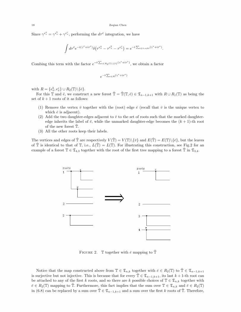
with R = {ebv, ecv} ∪R2(T)\{e}.For this T and e, we construct a new forest T = T(T, e) ∈ Tn−1,k+1 with R ∪ R1(T) as being the
set of k + 1 roots of it as follows:
(1) Remove the vertex v together with the (root) edge e (recall that v is the unique vertex towhich e is adjacent).
(2) Add the two daughter-edges adjacent to v to the set of roots such that the marked daughter-edge inherits the label of e, while the unmarked daughter-edge becomes the (k + 1)-th root
of the new forest T.(3) All the other roots keep their labels.
The vertices and edges of T are respectively V (T) = V (T)\{v} and E(T) = E(T)\{e}, but the leaves
of T is identical to that of T, i.e., L(T) = L(T). For illustrating this construction, see Fig.2 for an
example of a forest T ∈ T4,3 together with the root of the first tree mapping to a forest T in T3,4.
Figure 2. T together with e mapping to T
Notice that the map constructed above from T ∈ Tn,k together with e ∈ R2(T) to T ∈ Tn−1,k+1
is surjective but not injective. This is because that for every T ∈ Tn−1,k+1, its last k + 1-th root canbe attached to any of the first k roots, and so there are k possible choices of T ∈ Tn,k together with
e ∈ R2(T) mapping to T. Furthermore, this fact implies that the sum over T ∈ Tn,k and e ∈ R2(T)
in (6.8) can be replaced by a sum over T ∈ Tn−1,k+1 and a sum over the first k roots of T. Therefore,

Navier-Stokes equation 19
using these notations we can rewrite (6.8) as
B(~pk) = −k∑j=1
∫d~pk+1
[ k∏ι6=j
δ(pι − pι)]δ(pj − pj − pk+1
)Kj,k+1
×∑
T∈Tn−1,k+1
∫d~rn+k
1
(k + n)!
∑π2∈Πk+n
∏e∈R1(T)=L1(T)
e−tp2π1(e)δ(pπ1(e) − rπ2(e))
×∫ ∏
e∈E2(T)
dτedqeKπ2
T u(n+k)(~rn+k)∏
e∈R2(T)
e−t(γe+iτe)δ(qe − pπ1(e))
∏e∈L2(T)
δ(qe − rπ2(e))
×∏
e∈E2(T)
1
γe − q2e + iτe
∏v∈V (T)
δ(τeav − τe
bv − τe
cv)δ(qeav − qebv − qecv
)= W (k)Ξ
(k+1)n−1,t(~pk)
where we have rewritten the integration over dqe with e ∈ v in the second line of (6.8), so that itcorresponds to the action of the operator W (k) as defined in (4.10). This proves (6.5).
Finally, we turn to showing how to make the calculation in (6.6) rigorous. To this end, we introducea regularizing factor exp{−ε
∑e∈E2(T) |τe|} in the definition of GT,t in (5.7) for any ε > 0, denoted by
GT,t;ε this new kernel, and obtain the corresponding operator Ξ(k)n,t;ε. Then the proceeding calculation
for Ξ(k)n,t;ε in place of Ξ
(k)n,t can be done rigorously, and we have
Ξ(k)n,t(~pk) = lim
ε→0
∫ t
0
ds[− ~p2
kΞ(k)n,s;ε(~pk) +W (k)Ξ
(k+1)n−1,s;ε(~pk)
].
By Proposition 5.7, the integrations over τ -variables in Ξ(k)n,t;ε are all absolutely convergent uniformly
for every ε > 0 and for all t ∈ [0, T ] with any fixed T > 0. Thus, taking the limit ε → 0 on the righthand side of the above equation into the integral, we obtain
Ξ(k)n,t(~pk) =
∫ t
0
ds[− ~p2
kΞ(k)n,s(~pk) +W (k)Ξ
(k+1)n−1,s(~pk)
]which is equivalent to the equation (6.5), since Ξ
(k)n,0(~pk) = 0 as shown above. �
Next, we consider the error terms in (4.3).
Theorem 6.2. Let k ≥ 1 and n ≥ 1. For any given T > 0, if u(k+n) ∈ L2([0, T ],H1(k+n)) then
−∑
T∈Tn,k
∫ t
0
dsRT,t−su(k+n)(s) =
∫ t
0
dt1
∫ t1
0
dt2 · · ·∫ tn−1
0
dtnT (k)(t− t1)W (k) · · ·
× T (k+n−1)(tn−1 − tn)W (k+n−1)u(k+n)(tn)
(6.9)
for all t ∈ [0, T ].
Proof. Assume that k ≥ 1 and n ≥ 1. Fix T > 0. For any u(k+n) ∈ L2([0, T ],H1(k+n)) we put
Q(k)n (t)u(k+n) :=
∫ t
0
dt1
∫ t1
0
dt2 · · ·∫ tn−1
0
dtnT (k)(t− t1)W (k) · · ·
× T (k+n−1)(tn−1 − tn)W (k+n−1)u(k+n)(tn)
for all t ∈ [0, T ]. By Fubini’s theorem, we have
Q(k)n (t)u(k+n) =
∫ t
0
ds
[ ∫ t−s
0
dt1
∫ t1
0
dt2 · · ·∫ tn−2
0
dtn−1T (k)(t− s− t1)W (k) · · ·
× T (k+n−2)(tn−2 − tn−1)W (k+n−2)T (k+n−1)(tn−1)
]W (k+n−1)u(k+n)(s).
By (6.3), we have
(6.10) Q(k)n (t)u(k+n) =
∫ t
0
ds∑
T∈Tn−1,k
CT,t−sW(k+n−1)u(k+n)(s).
20 Zeqian Chen
Furthermore, by (5.7) and (4.10) we have, in momentum space,
Q(k)n (t)u(k+n)(~pk)
= −∫ t
0
ds∑
T∈Tn−1,k
∫d~rk+n−1
(k + n− 1)!
∑π2∈Πk+n−1
∏e∈R1(T)=L1(T)
e−(t−s)p2π1(e)δ(pπ1(e) − rπ2(e))
×∫ ∏
e∈E2(T)
dqedτe∏
e∈R2(T)
e−(t−s)(γe+iτe)δ(qe − pπ1(e))∏
e∈L2(T)
δ(qe − rπ2(e))
×∏
e∈E2(T)
1
γe − q2e + iτe
∏v∈V (T)
δ(τeav − τe
bv − τe
cv)δ(qeav − qebv − qecv
)
×Kπ2
T
[ k+n−1∑j=1
∫d~qk+1
[ k+n−1∏ι6=j
δ(rι − qι)]δ(rj − qj − qk+n
)Kj,k+nu
(n+k)(s, ~qn+k)
](6.11)
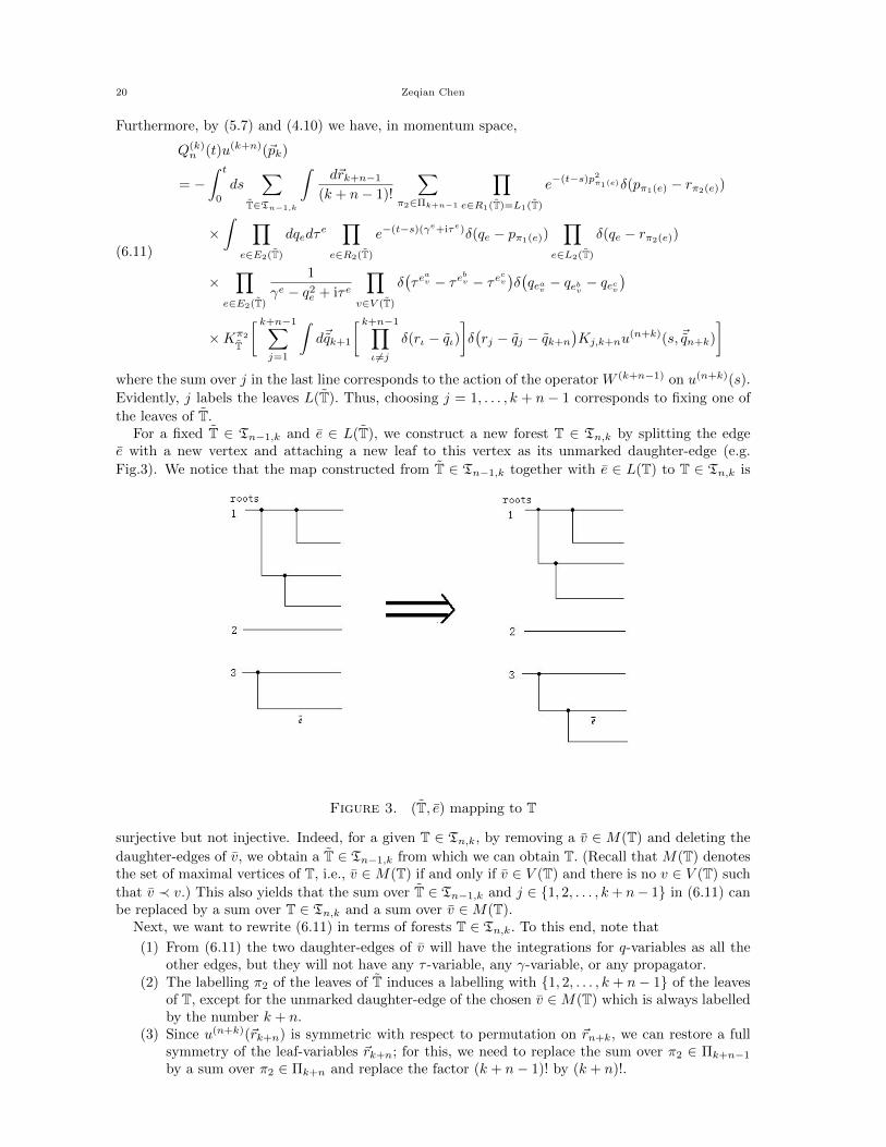
where the sum over j in the last line corresponds to the action of the operator W (k+n−1) on u(n+k)(s).
Evidently, j labels the leaves L(T). Thus, choosing j = 1, . . . , k + n − 1 corresponds to fixing one of
the leaves of T.For a fixed T ∈ Tn−1,k and e ∈ L(T), we construct a new forest T ∈ Tn,k by splitting the edge
e with a new vertex and attaching a new leaf to this vertex as its unmarked daughter-edge (e.g.
Fig.3). We notice that the map constructed from T ∈ Tn−1,k together with e ∈ L(T) to T ∈ Tn,k is
Figure 3. (T, e) mapping to T
surjective but not injective. Indeed, for a given T ∈ Tn,k, by removing a v ∈ M(T) and deleting the
daughter-edges of v, we obtain a T ∈ Tn−1,k from which we can obtain T. (Recall that M(T) denotesthe set of maximal vertices of T, i.e., v ∈M(T) if and only if v ∈ V (T) and there is no v ∈ V (T) such
that v ≺ v.) This also yields that the sum over T ∈ Tn−1,k and j ∈ {1, 2, . . . , k+ n− 1} in (6.11) canbe replaced by a sum over T ∈ Tn,k and a sum over v ∈M(T).
Next, we want to rewrite (6.11) in terms of forests T ∈ Tn,k. To this end, note that
(1) From (6.11) the two daughter-edges of v will have the integrations for q-variables as all theother edges, but they will not have any τ -variable, any γ-variable, or any propagator.
(2) The labelling π2 of the leaves of T induces a labelling with {1, 2, . . . , k + n− 1} of the leavesof T, except for the unmarked daughter-edge of the chosen v ∈M(T) which is always labelledby the number k + n.
(3) Since u(n+k)(~rk+n) is symmetric with respect to permutation on ~rn+k, we can restore a fullsymmetry of the leaf-variables ~rk+n; for this, we need to replace the sum over π2 ∈ Πk+n−1
by a sum over π2 ∈ Πk+n and replace the factor (k + n− 1)! by (k + n)!.

Navier-Stokes equation 21
Thus, we can rewrite (6.11) as
Q(k)n (t)u(k+n)(~pk)
=−∫ t
0
ds∑
T∈Tn,k
∑π2∈Πk+n
∑v∈M(T)
∫d~rn+k
(k + n)!
∏e∈R1(T)=L1(T)
e−(t−s)p2π1(e)δ(pπ1(e) − rπ2(e))
×∫ ∏
e∈E2(T)
dqe∏
e∈E2(T)e/∈Dv
dτe
γe − q2e + iτe
Kπ2
T u(n+k)(s, ~rn+k)∏
e∈R2(T)
e−(t−s)(γe+iτe)δ(qe − pπ1(e))
×∏
e∈L2(T)
δ(qe − rπ2(e))∏
v∈V (T)v 6=v
δ(τeav − τe
bv − τe
cv) ∏v∈V (T)
δ(qeav − qebv − qecv
)
=−∑
T∈Tn,k
∫ t
0
dsRT,t−su(k+n)(s)
where Dv denotes the set of daughter-edges of v. The proof is complete. �
In conclusion, combining Theorems 6.1 and 6.2 yields the expression (6.1).
7. A prior space-time estimates
In this section, we first present a prior space-time estimates for interaction operators CT,t and RT,t,and then give the proof of Theorem 4.1.
7.1. Space-time estimates for collision operators. We have a prior space-time estimates forCT,t as follows.
Theorem 7.1. Fix α > 12 and k ≥ 1. Let M > 0. Then there exists a constant C > 0 depending only
on α, k such that for any v(k) ∈ S(k)(R3) satisfying
(7.1) sup1≤i1,...,ik≤3
supp1,...,pk∈R3
〈p1〉3 · · · 〈pk〉3|v(k)i1,...,ik
(~pk)| ≤M,
for any n ≥ 0, and for all T ∈ Tn,k, we have
(7.2)∣∣⟨v(k), CT,tu
(n+k)⟩L2
(k)
∣∣ ≤MCn∥∥u(n+k)
∥∥Hα
(n+k)
for all u(n+k) ∈ Hα(n+k) and any 0 < t ≤ 1.
Proof. Fix k ≥ 1 and 0 < t ≤ 1. Let M > 0. Assume that v(k) ∈ S(k)(R3) satisfying (7.1). Let
T ∈ Tn,k and suppose u(n+k) ∈ L2(n+k). We have, by the definition of CT,tu
(n+k) in (5.6),
⟨v(k), CT,tu
(n+k)⟩L2
(k)
=1
(k + n)!
∑π2∈Πk+n
∫d~pkd~rn+k
∏e∈R1(T)=L1(T)
e−tp2π1(e)δ(pπ1(e) − rπ2(e))
×∫ ∏
e∈E2(T)
dτedqe
[ ∑1≤i1,...,ik≤3
v(k)i1,...,ik
(~pk)Kπ2
T u(n+k)i1,...,ik
(~rn+k)
]×
∏e∈R2(T)
e−t(γe+iτe)δ(qe − pπ1(e))
∏e∈L2(T)
δ(qe − rπ2(e))
×∏
e∈E2(T)
1
γe − q2e + iτe
∏v∈V (T)
δ(τeav − τe
bv − τe
cv)δ(qeav − qebv − qecv
).
For simplicity, we will write E = E(T), R2 = R2(T), L1 = L1(T), etc. Since u(n+k)(~rn+k) is symmetrywith respect to the permutation on ~rn+k, the integral on the right-hand side of the above equationhas the same value for every π2 ∈ Πn+k, and hence, instead of averaging over π2, we fix one π2 so

22 Zeqian Chen
that π2(e) ≥ |R1|+ 1 for all e ∈ L2. Then, using all the δ-functions and integrating over the variables~pk and ~rn+k, one has∣∣⟨v(k), CT,tu
(n+k)⟩L2
(k)
∣∣ ≤Me−t∑e∈R2
γe∫ ∏
e∈Edqe
∏e∈E2
dτe∏e∈E2
1
|γe − q2e + iτe|
∏e∈R
1
〈qe〉3
×∏v∈V
δ(τeav − τe
bv − τe
cv)δ(qeav − qebv − qecv
) ∑1≤i1,...,ik≤3
|Kπ2
T u(n+k)i1,...,ik
(qe : e ∈ L)|
where we have used the assumption (7.1), and the permutation symmetry of u(n+k), namely, u(n+k)
depends only on the set of the variables qe associated with the leaves of T, but not on the order ofthose variables.
Choosing γe = − 1t for all e ∈ L2, we have that γe ≤ − 1
t for every e ∈ E2, and∑e∈R2
γe = −(n+ |R2|)1
t.
Moreover, by the definition of Kπ2
T u(n+k) (see (5.2) and (5.3)), we have
(7.3) |Kπ2
T u(n+k)i1,...,ik
(qe)| ≤ 6n∏v∈V|qebv + qecv |
∑1≤j|R1|+1,...,jn+k≤3
∣∣u(n+k)i1,...,i|R1|,j|R1|+1,...,jn+k
(qe)∣∣.
Then for a fixed α > 12 ,∣∣⟨v(k), CT,tu
(n+k)⟩L2
(k)
∣∣ ≤MCn∫ ∏
e∈Edqe
∏e∈E2
dτe∏e∈E2
1
|( 1t + q2
e)i + τe|∏e∈R
1
〈qe〉3
×∏v∈V
δ(τeav − τe
bv − τe
cv)δ(qeav − qebv − qecv
)|qebv + qecv |
∑1≤i1,...,in+k≤3
∣∣u(n+k)i1,...,in+k
(qe : e ∈ L)∣∣
≤ Cn∥∥u(k+n))
∥∥Hα
(k+n)
(∫ ∏e∈L2
dqe(1 + |qe|2)α
[ ∫ ∏e∈E\L
dqe∏e∈E2
dτe∏e∈R2
1
〈qe〉3
×∏e∈E2
1
|(1 + q2e)i + τe|
∏v∈V
δ(τeav − τe
bv − τe
cv)δ(qeav − qebv − qecv
)|qebv + qecv |
]2) 12
(7.4)
where C > 0 in the second line is a constant depending only on α, k. Here, we have used the conditions0 < t ≤ 1, the Cauchy-Schwarz inequality and the integral
∫ ∏e∈L1=R1
1(1+|qe|2)α〈qe〉6 dqe <∞.
Next, we estimate the following integral (note that E\L = E2\L2)
I =
∫ ∏e∈E2\L2
dqe∏e∈E2
dτe∏e∈E2
1
|(1 + q2e)i + τe|
∏e∈R2
1
〈qe〉3
×∏v∈V
δ(τeav − τe
bv − τe
cv)δ(qeav − qebv − qecv
)|qebv + qecv |.
(7.5)
For bounding the integral (7.5), we first successively integrate over all τ -variables and then over allmomenta except for the momenta of the leaves.
First of all, we claim that∫ ∏e∈E2
dτe
|(1 + q2e)i + τe|
∏v∈V
δ(τeav − τe
bv − τe
cv)
.ε∏
v: eav /∈R2
1
(1 + q2ebv
+ q2ecv
)1−ε
∏v: eav∈R2
1
(1 + q2eav
+ q2ebv
+ q2ecv
)1−ε .(7.6)
where ε is a small constant which will be specified later.Note that the delta functions relate variables within the same trees, the integration then can be
done independently in each tree of T. The order of integration is prescribed according to the converseorder of vertices of the trees (see Appendix 9.1 below), that is, the τ -variables of a vertex v will beintegrated only when those of all vertices v′ with v ≺ v′ have already been integrated out.
Now, we choose a vertex v ∈ V and suppose that the τ -integrations over all v′ � v have beenperformed. We will perform the integration over the τ -variables associated with the daughter-edges

Navier-Stokes equation 23
of the vertex v. We need to distinguish two cases according to whether the mother-edge of v, eav (withthe notation of Fig.1), is the root or not.• eav is not a root: 1) Both ebv and ecv are leaves. By Lemma 9.9 one has∫
dτ bdτ cδ(τa − τ b − τ c)|(1 + q2
b )i + τ b||(1 + q2c )i + τ c|
=
∫dτ b
|(1 + q2b )i + τ b||(1 + q2
c )i + τa − τ b|
.ε1
|τa + (1 + q2b + q2
c )i|1−ε
for all τa ∈ R and all qb, qc ∈ R3.2) One of ebv and ecv is a leaf. Assuming that there exists v′ such that v′ � v with eav′ = ecv and ebv
is a leaf, we have ∫dτ bdτ cδ(τa − τ b − τ c)
|(1 + q2b )i + τ b||(1 + q2
c )i + τ c||(1 + q2b′ + q2
c′)i + τ c|1−ε
≤ 1
(1 + q2b′ + q2
c′)1−ε
∫dτ c
|(1 + q2b )i + τa − τ c||(1 + q2
c )i + τ c|
≤ 1
(1 + q2b′ + q2
c′)1−ε
1
|τa + (1 + q2b + q2
c )i|1−ε.
Similarly, the same inequality holds when eav′ = ebv and ecv is a leaf.3) Neither ebv nor ecv is a leaf, i.e.,there are v′, v′′ � v such that ebv = eav′ and ecv = eav′′ . Then we
have ∫dτ bdτ cδ(τa − τ b − τ c)
|(1 + q2b )i + τ b||(1 + q2
c )i + τ c||(1 + q2b′ + q2
c′)i + τ b|1−ε|(1 + q2b′′ + q2
c′′)i + τ c|1−ε
≤ 1
(1 + q2b′ + q2
c′)1−ε(1 + q2
b′′ + q2c′′)
1−ε
∫dτ c
|(1 + q2b )i + τa − τ c||(1 + q2
c )i + τ c|
≤ 1
(1 + q2b′ + q2
c′)1−ε(1 + q2
b′′ + q2c′′)
1−ε1
|τa + (1 + q2b + q2
c )i|1−ε.
• eav is a root: In this case, we will integrate over all the τ -variables associated with the edges ofthe vertex including the mother-edge. We have three different cases yet.
1) Both ebv and ecv are leaves. In this case, we have∫dτadτ bdτ cδ(τa − τ b − τ c)
|(1 + q2a)i + τa||(1 + q2
b )i + τ b||(1 + q2c )i + τ c|
=
∫dτadτ b
|(1 + q2a)i + τa||(1 + q2
b )i + τ b||(1 + q2c )i + τa − τ b|
.ε1
(1 + q2a + q2
b + q2c )1−ε
where we have used Lemma 9.9 twice.2) One of ebv and ecv is a leaf. Suppose that there exists v′ such that v′ � v with eav′ = ecv and ebv is
a leaf, we have∫dτadτ bdτ cδ(τa − τ b − τ c)
|(1 + q2a)i + τa||(1 + q2
b )i + τ b||(1 + q2c )i + τ c||(1 + q2
b′ + q2c′)i + τ c|1−ε
≤ 1
(1 + q2b′ + q2
c′)1−ε
∫dτadτ c
|(1 + q2a)i + τa||(1 + q2
b )i + τa − τ c||(1 + q2c )i + τ c|
.ε1
(1 + q2b′ + q2
c′)1−ε
1
(1 + q2a + q2
b + q2c )1−ε .
Similarly, the same inequality holds when eav′ = ebv and ecv is a leaf.

24 Zeqian Chen
3) Neither ebv nor ecv is a leaf, i.e., there are v′, v′′ � v such that ebv = eav′ and ecv = eav′′ . Then wehave∫
dτadτ bdτ cδ(τa − τ b − τ c)|(1 + q2
a)i + τa||(1 + q2b )i + τ b||(1 + q2
c )i + τ c||(1 + q2b′ + q2
c′)i + τ b|1−ε|(1 + q2b′′ + q2
c′′)i + τ c|1−ε
≤ 1
(1 + q2b′ + q2
c′)1−ε(1 + q2
b′′ + q2c′′)
1−ε
∫dτadτ c
|(1 + q2a)i + τa||(1 + q2
b )i + τa − τ c||(1 + q2c )i + τ c|
.ε1
(1 + q2b′ + q2
c′)1−ε(1 + q2
b′′ + q2c′′)
1−ε1
(1 + q2a + q2
b + q2c )1−ε .
In summary, we have proven (7.6).Then, by (7.6) we have
I .ε
∫ ∏e∈E2\L2
dqe∏v∈V
δ(qeav − qebv − qecv
) ∏e∈R2
1
〈qe〉3
×∏
v: eav /∈R2
|qebv + qecv |(1 + q2
ebv+ q2
ecv)1−ε
∏v: eav∈R2
|qebv + qecv |(1 + q2
eav+ q2
ebv+ q2
ecv)1−ε .
Thus we have∣∣⟨v(k), CT,tu(n+k)
⟩L2
(k)
∣∣ ≤MCn∥∥u(k+n))
∥∥Hα
(k+n)
(∫ ∏e∈E2
dqe∏v∈V
δ(qeav − qebv − qecv
) ∏e∈L2
1
(1 + |qe|2)α
×∏e∈R2
1
〈qe〉6∏
v: eav /∈R2
|qebv + qecv |2
(1 + q2ebv
+ q2ecv
)2(1−ε)
∏v: eav∈R2
|qebv + qecv |2
(1 + q2eav
+ q2ebv
+ q2ecv
)2(1−ε)
) 12
where C > 0 is a constant depending only on α, k, and ε.It remains to estimate the momenta integrations
Ξ =
∫ ∏e∈E2
dqe∏v∈V
δ(qeav − qebv − qecv
) ∏e∈L2
1
(1 + |qe|2)α
∏e∈R2
1
〈qe〉6
×∏
v: eav /∈R2
|qebv + qecv |2
(1 + q2ebv
+ q2ecv
)2(1−ε)
∏v: eav∈R2
|qebv + qecv |2
(1 + q2eav
+ q2ebv
+ q2ecv
)2(1−ε) .
Since the delta functions relate variables within the same trees, we only need to consider the integrationover all q-variables associated with a tree T, that is
Ξ(T) =
∫ ∏e∈E2(T)
dqe∏
v∈V (T)
δ(qeav − qebv − qecv
) 1
〈qR(T)〉6|qebv + qecv |
2
(1 + q2eav=R(T) + q2
ebv+ q2
ecv)2(1−ε)
×∏
e∈L2(T)
1
(1 + |qe|2)α
∏v∈V (T): eav 6=R(T)
|qebv + qecv |2
(1 + q2ebv
+ q2ecv
)2(1−ε) .
(7.7)
Again, we begin the integration with the q-variables of the leaves and proceed toward the root, anda vertex v will be integrated only when all vertices v′ with v ≺ v′ have already been integrated out.
Indeed, for a maximal vertex v whose two daughter edges must be leaves, if eav 6= R then theassociated integration is
Ξv =
∫dqebvdqecvδ
(qeav − qebv − qecv
) 1
(1 + |qebv |2)α
1
(1 + |qecv |2)α|qebv + qecv |
2
(1 + q2ebv
+ q2ecv
)2(1−ε)
=
∫dqebv
1
(1 + |qebv |2)α
1
(1 + |qeav − qebv |2)α
|qeav |2
(1 + q2ebv
+ (qeav − qebv )2)2(1−ε) .
Taking ε = 14 min{1, α− 1
2} > 0 (noticing that α > 12 ), we claim that there exists a constant Cα > 0
depending only on α such that
(7.8) Ξv ≤ Cα1
(1 + |qeav |2)α.

Navier-Stokes equation 25
For proving this inequality, noticing that q2eav. q2
ebv+ (qeav − qebv )2, we have
q2eav
(1 + q2ebv
+ (qeav − qebv )2)2(1−ε) .1
[q2ebv
+ (qeav − qebv )2]1−2ε.
Thus
Ξv .1
(1 + |qeav |2)α
∫dqebv
(1 + q2ebv
+ (qeav − qebv )2)α
(1 + |qebv |2)α(1 + |qeav − qebv |
2)α1
(q2ebv
+ (qeav − qebv )2)1−2ε
≤ Cα(1 + |qeav |2)α
∫dqebv
1
(1 + |qebv |2)α|qebv |
2(1−2ε)≤ Cα
(1 + |qeav |2)α
provided α > 12 and ε = 1
4 min{1, α− 12} > 0. This completes the proof of the inequality (7.8).
Subsequently, every vertex v for which all vertices v′ with v ≺ v′ have already been integrated outis associated with the integration of the form Ξv as above when eav 6= R. Thus, we obtain
Ξ(T) ≤ C |V (T)|−1α
∫dqeav=R(T)dqebvdqecvδ
(qeav − qebv − qecv
) 1
〈qR(T)〉6
×|qebv + qecv |
2
(1 + q2eav=R(T) + q2
ebv+ q2
ecv)2(1−ε)
1
(1 + |qebv |2)α
1
(1 + |qecv |2)α≤ C |V (T)|
α .
Therefore, we conclude that
Ξ =∏T∈T
Ξ(T) ≤ Cnα .
This completes the proof. �
7.2. Space-time estimates for error operators. In this subsection, we prove a space-time esti-mate for the error term RT,t.
Theorem 7.2. Fix k ≥ 1. Let M > 0. Then there exists a constant C > 0 depending only on k suchthat for any v(k) ∈ S(k)(R3) satisfying (7.1) with the bound M, for any n ≥ 0 and any T ∈ Tn,k, wehave
(7.9)∣∣⟨v(k), RT,tu
(n+k)⟩L2
(k)
∣∣ ≤MCntn2−1
∥∥u(n+k)∥∥H1
(n+k)
for all u(n+k) ∈ H1(n+k) and any 0 < t ≤ 1.
Proof. By (5.9), we have⟨v(k), RT,tu
(n+k)⟩L2
(k)
=1
(k + n)!
∑π2∈Πk+n
∫d~pkd~rn+k
∑v∈M(T)
∏e∈R1(T)=L1(T)
e−tp2π1(e)δ(pπ1(e) − rπ2(e))
×∫ ∏
e∈E2(T)
dqe∏
e∈E2(T)e/∈Dv
dτe
γe − q2e + iτe
[ ∑1≤i1,...,ik≤3
v(k)i1,...,ik
(~pk)Kπ2
T u(n+k)i1,...,ik
(~rn+k)
]
×∏
e∈R2(T)
e−t(γe+iτe)δ(qe − pπ1(e))
∏e∈L2(T)
δ(qe − rπ2(e))
×∏
v∈V (T)v 6=v
δ(τeav − τe
bv − τe
cv) ∏v∈V (T)
δ(qeav − qebv − qecv
).
Recall that M(T) is the set of maximal elements in V (T) and Dv denotes the set of daughter-edgesfor a vertex v ∈ M(T). In the integration of the right hand side of the above equation, if thereexists a v ∈ M(T) such that eav ∈ R(T), then there is only one denominator containing τe in theintegral for this tree, and so the associated τe-integral would not be absolutely convergent. In this
case, using (5.4), we perform the integration over the τeav and then obtain a factor e
−tq2eav . Denote
by E2(T, v) = E2(T)\{eav} if eav ∈ R(T), and otherwise E2(T, v) = E2(T). After performing theintegration over τe associated to e /∈ E2(T, v), we take the absolute value of the above integrand.

26 Zeqian Chen
As done in the proof of Theorem 7.1, instead of averaging over π2, we fix one π2 so that π2(e) ≥|R1|+ 1 for all e ∈ L2. Then by (7.3), we obtain that (noticing that γe = − 1
t for all e ∈ L2)
∣∣⟨v(k), RT,tu(n+k)
⟩L2
(k)
∣∣ ≤MCn∑
v∈M(T)
∫ ∏e∈E
dqe∏
e∈E2(T,v)e/∈Dv
dτe
|( 1t + q2
e)i + τe|∏e∈R
1
〈qe〉3
×∏
v∈V (T)v 6=v
δ(τeav − τe
bv − τe
cv) ∏v∈V
δ(qeav−qebv − qecv
)|qebv + qecv |
∑1≤i1,...,in+k≤3
∣∣u(n+k)i1,...,in+k
(qe : e ∈ L)∣∣
≤MCn∥∥u(k+n))
∥∥H1
(k+n)
∑v∈M(T)
(∫ ∏e∈L2
dqe〈qe〉2
[ ∫ ∏e∈E2\L2
dqe∏
e∈E2(T,v)e/∈Dv
dτe
|( 1t + q2
e)i + τe|
×∏e∈R2
1
〈qe〉3∏
v∈V (T)v 6=v
δ(τeav − τe
bv − τe
cv) ∏v∈V
δ(qeav − qebv − qecv
)|qebv + qecv |
]2) 12
where C > 0 depends only on k.Making variable substitution as qe −→ t−
12 qe for all e ∈ E2\L2, and τe −→ t−1τe for all e ∈
E2(T, v)\Dv, we have
dτe
|(1/t+ q2e)i + τe|
−→ dτe
|(1 + q2e)i + τe|
,
δ(τeav − τe
bv − τe
cv)−→ tδ
(τeav − τe
bv − τe
cv),
δ(qeav − qebv − qecv
)−→ t
32 δ(qeav − qebv − qecv
).
Then ∣∣⟨v(k), RT,tu(n+k)
⟩L2
(k)
∣∣ ≤MCntn2−1
∥∥u(k+n))∥∥H1
(k+n)
×∑
v∈M(T)
(∫ ∏e∈L2
dqe〈qe〉2
[ ∫ ∏e∈E2\L2
dqe∏
e∈E2(T,v)e/∈Dv
dτe
|(1 + q2e)i + τe|
∏e∈R2
1
〈t− 12 qe〉3
×∏
v∈V (T)v 6=v
δ(τeav − τe
bv − τe
cv) ∏v∈V
δ(qeav − qebv − qecv
)|qebv + qecv |
]2) 12
.
We first estimate Iv, where
Iv =
∫ ∏e∈E2\L2
dqe∏
e∈E2(T,v)e/∈Dv
dτe
|(1 + q2e)i + τe|
∏e∈R2
1
〈t− 12 qe〉3
×∏
v∈V (T)v 6=v
δ(τeav − τe
bv − τe
cv) ∏v∈V
δ(qeav − qebv − qecv
)|qebv + qecv |.
Given 0 < ε < 1 which will be fixed later, as done in the proof of Theorem 7.1, we perform integrationsover all τ -variables and then obtain
Iv .ε
∫ ∏e∈E2\L2
dqe∏v∈V
δ(qeav − qebv − qecv
) ∏e∈R2
1
〈t− 12 qe〉3
× |qebv + qecv |∏
v: eav /∈R2
v 6=v
|qebv + qecv |(1 + q2
ebv+ q2
ecv)1−ε
∏v: eav∈R2
v 6=v
|qebv + qecv |(1 + q2
eav+ q2
ebv+ q2
ecv)1−ε .
Navier-Stokes equation 27
Thus,∣∣⟨v(k), RT,tu(n+k)
⟩L2
(k)
∣∣ ≤MCntn2−1
∥∥u(k+n))∥∥H1
(k+n)
×∑
v∈M(T)
(∫ ∏e∈E2
dqe∏v∈V
δ(qeav − qebv − qecv
) ∏e∈L2
1
〈qe〉2∏e∈R2
1
〈t− 12 qe〉6
×|qebv + qecv |2
∏v: eav /∈R2
v 6=v
|qebv + qecv |2
(1 + q2ebv
+ q2ecv
)2(1−ε)
∏v: eav∈R2
v 6=v
|qebv + qecv |2
(1 + q2eav
+ q2ebv
+ q2ecv
)2(1−ε)
) 12
.
Next, we estimate the integration on the right hand side of the above inequality. Fix v ∈ M(T)and denote the integration by Ξ(T, v), i.e.,
Ξ(T, v) =
∫ ∏e∈E2
dqe∏v∈V
δ(qeav − qebv − qecv
) ∏e∈L2
1
〈qe〉2∏e∈R2
1
〈t− 12 qe〉6
× |qebv + qecv |2
∏v: eav /∈R2
v 6=v
|qebv + qecv |2
(1 + q2ebv
+ q2ecv
)2(1−ε)
∏v: eav∈R2
v 6=v
|qebv + qecv |2
(1 + q2eav
+ q2ebv
+ q2ecv
)2(1−ε) .
Since the delta functions relate variables within the same trees, we may consider separately theintegrations over all q-variables associated with each tree. Note that the integration associated witha tree T not including v is the same as Ξ(T) in (7.7) in the proof of Theorem 7.1 and so we haveΞ(T) ≤ C |V (T)|, where C is a absolute constant. Thus, it remains to estimate the integration overthe tree T containing v, which we denote by Ξ(T, v).
Note that
(7.10)
∫dqebvdqe
cv
δ(qeav − qebv − qecv )|qebv + qecv |2
〈qebv 〉2〈qecv 〉2
= |qeav |2
∫dqebv
〈qebv 〉2〈qeav − qebv 〉
2. |qeav |.
If eav = R(T), then
Ξ(T, v) =
∫dqeavdqebvdqe
cv
δ(qeav − qebv − qecv )|qebv + qecv |2
〈t− 12 qeav 〉6〈qebv 〉
2〈qecv 〉2.∫
1
〈qeav 〉5dqeav <∞
where we have used the fact that 〈t− 12 qeav 〉 ≥ 〈qeav 〉 (because 0 < t ≤ 1). It remains to deal with the
case eav 6= R(T), where
Ξ(T, v) =
∫ ∏e∈E2(T)
dqe∏
v∈V (T)
δ(qeav − qebv − qecv
) 1
〈t− 12 qR(T)〉6
|qebv + qecv |2
(1 + q2eav=R(T) + q2
ebv+ q2
ecv)2(1−ε)
×|qebv + qecv |2∏
e∈L2(T)
1
〈qe〉2∏
v∈V (T)\{v}eav 6=R(T)
|qebv + qecv |2
(1 + q2ebv
+ q2ecv
)2(1−ε) .
At first, for a maximal vertex v ∈ V (T)\{v} whose two daughter edges must be leaves, the associ-ated integration is
Ξv =
∫dqebvdqecvδ
(qeav − qebv − qecv
) 1
〈qebv 〉2
1
〈qecv 〉2|qebv + qecv |
2
(1 + q2ebv
+ q2ecv
)2(1−ε)
=
∫dqebv
1
〈qebv 〉2
1
〈qeav − qebv 〉2
|qeav |2
(1 + q2ebv
+ (qeav − qebv )2)2(1−ε) .
Taking 0 < ε ≤ 34 , we have
Ξv .1
〈qeav 〉2.
Subsequently, every vertex v with v ⊀ v for which all vertices v′ with v ≺ v′ have already beenintegrated out is associated with the integration of the form Ξv as above. On the other hand, by
28 Zeqian Chen
(7.10), the integration associated with v is
Ξv =
∫dqebvdqe
cvδ(qeav − qebv − qecv
) 1
〈qebv 〉2
1
〈qecv 〉2|qebv + qecv |
2 . 〈qeav 〉.
Secondly, suppose that v is a vertex with one of the leaves being eav , for instance ebv = eav . Ifeav 6= R(T), then the integration is
Ξv =
∫dqebvdqecvδ
(qeav − qebv − qecv
) 〈qebv 〉〈qecv 〉2
|qebv + qecv |2
(1 + q2ebv
+ q2ecv
)2(1−ε)
≤|qeav |2
∫dqebv
1
〈qeav − qebv 〉2
1
〈qebv 〉3−4ε
. |qeav |
provided 0 < ε ≤ 14 . Subsequently, for each v ≺ v with eav 6= R(T), the associated integration is the
same as this Ξv and so . |qeav |.Finally, we will arrive the vertex v ≺ v with eav = R(T). Then the integration is
Ξv =
∫dqeavdqebvdqecvδ
(qeav − qebv − qecv
) 1
〈t− 12 qR(T)〉6
〈qebv 〉〈qecv 〉2
|qebv + qecv |2
(1 + q2eav=R(T) + q2
ebv+ q2
ecv)2(1−ε)
≤∫dqeavdqebv
1
〈qR(T)〉4〈qebv 〉
〈qeav − qebv 〉2
1
(1 + q2eav=R(T) + q2
ebv+ (qeav − qebv )2)2(1−ε) ≤ C
for some absolute constant C <∞ uniformly for all 0 < ε ≤ 14 .
Thus, if 0 < ε ≤ 14 we have
Ξ(T, v) ≤ C |V (T)|
and hence
Ξ(T, v) = Ξ(T, v)∏v /∈T
Ξ(T) ≤ Cn
because V (T) = n. Note that |M(T)| ≤ n. Therefore, we conclude (7.9). �
7.3. Proof for uniqueness. We are now ready to prove Theorem 4.1. Let T > 0. For a given C > 0,
suppose that U1(t) = (u(k)1 (t))k≥1 and U2(t) = (u
(k)2 (t))k≥1 are two mild solutions in [0, T ] to the
hierarchy (3.18) such that U1(0) = U2(0), and for every i = 1, 2, u(k)i ∈ L∞([0, T ],H1
(k)) satisfying the
bound
‖u(k)i ‖L∞([0,T ],H1
(k)) ≤ Ck
for all k ≥ 1. We need to prove that U1(t) = U2(t) for every t ∈ [0, T ]. In fact, it suffices to prove that
for each fixed k ≥ 1, u(k)1 (t) = u
(k)2 (t) for all t ∈ [0, T ].
To this end, for a given k ≥ 1, we can expand u(k)i (t) (i = 1, 2) in a Duhamel expansion as in (4.3).
Then by Theorems 6.1 and 6.2, we have
u(k)i (t) = T (k)(t)u
(k)i (0) +
n−1∑m=1
∑T∈Tm,k
CT,tu(k+m)i (0)−
∑T∈Tn,k
∫ t
0
dsRT,t−su(k+n)i (s)(7.11)
for all n > 1, where i = 1, 2. For any v(k) ∈ S(k)(R3), one has
〈v(k), u(k)i (t)〉L2
(k)= 〈v(k), T (k)(t)u
(k)i (0)〉L2
(k)+
n−1∑m=1
∑T∈Tm,k
〈v(k), CT,tu(k+m)i (0)〉L2
(k)
−∑
T∈Tn,k
∫ t
0
ds〈v(k), RT,t−su(k+n)i (s)〉L2
(k)
for i = 1, 2. By Theorem 7.1, the terms in the sum over m are all finite. Since U1(0) = U2(0),
when taking the difference between 〈v(k), u(k)1 (t)〉L2
(k)and 〈v(k), u
(k)2 (t)〉L2
(k), the free evolution terms
Navier-Stokes equation 29
T (k)(t)u(k)i (0) and all the terms in the sum over m disappear, and so we have
〈v(k), u(k)1 (t)− u(k)
2 (t)〉L2(k)
= −∑
T∈Tn,k
∫ t
0
ds⟨v(k), RT,t−s[u
(k+n)1 (s)− u(k+n)
2 (s)]⟩L2
(k)
for any n > 1. Then for 0 < t ≤ 1 and n > 1, by Theorem 7.2 and the estimation |Tn,k| ≤ 23n+k (cf.(9.1)) we have∣∣〈v(k), u
(k)1 (t)− u(k)
2 (t)〉L2(k)
∣∣≤MCn
∫ t
0
ds(t− s)n2−1(‖u(k+n)
1 (s)‖H1(n+k)
+ ‖u(k+n)2 (s)‖H1
(n+k)
)≤MCnt
n2
where we have used the assumption that ‖u(n+k)i ‖L∞([0,T ],H1
(n+k)) ≤ Cn+k for i = 1, 2. Hence, taking
t = min{
12 ,
1(2C)2
}, we have ∣∣〈v(k), u
(k)1 (t)− u(k)
2 (t)〉L2(k)
∣∣ ≤M 1
2n.
Since n > 1 is arbitrary,
〈v(k), u(k)1 (t)− u(k)
2 (t)〉L2(k)
= 0
for any v(k) ∈ S(k)(R3), provided t ≤ min{
12 ,
1(2C)2
}. Thus, we conclude that u
(k)1 (t) = u
(k)2 (t) for all
t ≤ min{
12 ,
1(2C)2
}. By iteration, we can prove that u
(k)1 (t) = u
(k)2 (t) for all t ∈ [0, T ]. This completes
the proof of Theorem 4.1.
8. A solution formula for the incompressible Navier-Stokes equation
By (6.1), we have a formal formula for the solution to the Navier-Stokes hierarchy (3.10) with an
initial data U0 = (u(k)0 )k≥1 as follows
u(k)(t) = et4(k)
u(k)0 +
∞∑n=1
∑T∈Tn,k
CT,tu(n+k)0(8.1)
for every k ≥ 1, provided the remainder terms converge to zero as n→∞.The following is to prove such a formula for the Navier-Stokes equation (1.2) in H1(R3).
Theorem 8.1. Let u0 ∈ H1(R3) with5·u0 = 0. Let u be the unique weak solution in C([0, T ∗),H1(R3))for the initial problem of the Navier-Stokes equation{
∂tu = 4u−W (u⊗ u),
5 ·u = 0,
with the initial datum u(0) = u0, where T ∗ is the maximal life-time of u(t). Then there exits 0 < t∗ <T ∗ such that
(8.2) u(t) = et4u0 +
∞∑n=1
∑T∈Tn,1
CT,tu⊗n+1
0
in the sense of distributions for every 0 < t < t∗.
Proof. Fix 0 < T < T ∗. Then u(t) ∈ C([0, T ],H1(R3)) so that
CT = supt∈[0,T ]
‖u(t)‖H1 <∞.
Put u(k)(t) = u(t)⊗k
for every k ≥ 1, then by Corollary 4.3, (u(k)(t))k≥1 is the unique mild solution
for the Navier-Stokes hierarchy (3.18) with the initial datum u(k)(0) = u⊗k
0 , such that for every k ≥ 1,
u(k) ∈ L∞([0, T ],H1(k)) and satisfies the bound
sup0≤t≤T
‖u(k)(t)‖H1 ≤ CkT .

30 Zeqian Chen
On the other hand, it follows from (6.1) that for n > 1,
u(t) = et4u0 +
n−1∑j=1
∑T∈Tj,1
CT,tu⊗j+1
0 −∑
T∈Tn,1
∫ t
0
dsRT,t−su(n+1)(s)
for all 0 ≤ t ≤ T. As shown in the proof of Theorem 7.1, every term CT,tu⊗j+1
0 is well defined in thesense of distribution. It remains to prove that
limn→∞
∑T∈Tn,1
∫ t
0
dsAT,t−su(n+1)(s) = 0
in the sense of distributions for 0 < t < t∗, where t∗ will be fixed later.By Theorem 7.2, for any φ ∈ S(R3) we have
|〈φ,AT,t−su(n+1)(s)〉| ≤MφC
n0 (t− s)n2−1‖u(n+1)(s)‖H1
(n+1)
for t, s ∈ (0, T ] so that 0 < t − s ≤ 1, where Mφ is a positive constant depending only on φ, andC0 > 0 is an absolute constant. Then∣∣∣⟨φ, ∑
T∈Tn,1
∫ t
0
dsAT,t−su(n+1)(s)
⟩∣∣∣ ≤MφCn0 23n+1
∫ t
0
ds(t− s)n2−1‖u(n+1)(s)‖H1(n+1)
≤MφCn0 23n+1Cn+1
T tn2 .
Thus, choosing t∗ = min{1, (8C0CT )−2}, we have
limn→∞
⟨φ,
∑T∈Tn,1
∫ t
0
dsAT,t−su(n+1)(s)
⟩= 0
for all 0 < t < t∗. This proves (8.2). �
Remark 8.2. (1) Note that each CT,t with T ∈ Tn,1 is a multi-parameter integral operator withan explicit kernel (5.7) in momentum space, which describes a kind of processes of two-bodyinteraction of n+1 “particles”. Thus, the formula (8.2) may be regarded as an explicit expressionof solution to the homogeneous, incompressible Navier-Stokes equation (1.1) in R3, and shouldbe useful for computing this solution.
(2) A natural question is whether t∗ can be taken as being T ∗, that is, whether the formula (8.2)holds true for all 0 < t < T ∗ ? For checking this problem, it seems to need new ideas beyond theargument in the above proof.
Furthermore, we can prove stronger convergence of the series in (8.2) if the initial data have higherregularity.
Theorem 8.3. Let β < − 32 and let α > 3
2 . Let u0 ∈ Hα(R3) with 5 · u0 = 0, and let u be the unique
weak solution in C([0, T ∗),Hα(R3)) for the initial problem of the Navier-Stokes equation (1.2) withthe initial datum u(0) = u0, where T ∗ is the maximal life-time of u(t). Then there exits 0 < t∗ < T ∗
such that (8.2) holds in Hβ(R3) for all 0 < t < t∗.
The proof is based on a prior space-time estimates for the interaction operators in multi-parameterSobolev spaces as follows, which are of their own interest.
Proposition 8.4. Fix β ∈ R and α > max{ 12 , β+ 3
2}. Then there exists a constant C > 0, dependingonly on α and β, such that for every k ≥ 1, n ≥ 0, and any T ∈ Tn,k, one has
(8.3)∥∥CT,tu
(n+k)∥∥Hβ
(k)
≤ Ck+ntδn∥∥u(n+k)
∥∥Hα
(n+k)
for all u(n+k) ∈ Hα(n+k) and any t > 0, where δ = 14 min{1, α− 1
2}.
Proposition 8.5. Fix β < − 32 and α > 3
2 . Then there exists a constant C > 0, depending only on αand β, such that for every k ≥ 1, n ≥ 1, and any T ∈ Tn,k, one has
(8.4)∥∥RT,tu
(n+k)∥∥Hβ
(k)
≤ Ck+ntδn∥∥u(n+k)
∥∥Hα
(n+k)
for all u(n+k) ∈ Hα(n+k) and any 0 < t ≤ 1, where δ = 14 min{1, α− 3
2}.

Navier-Stokes equation 31
Proof of Theorem 8.3. We can proceed the same argument in the proof of Theorem 8.1, with thehelp of Propositions 8.4 and 8.5 in the case k = 1. The details are omitted. �
We next turn to the proofs of Propositions 8.4 and 8.5, which follow the argument in the ones ofTheorems 7.1 and 7.2. First of all, we prove (8.3) on a prior space-time estimates of collision operatorsin Sobolev spaces.
Proof of Proposition 8.4. Fix β ∈ R and α > max{ 12 , β + 3
2}. Let k ≥ 1 and t > 0. Let T ∈ Tn,kand suppose u(n+k) ∈ L2
(n+k). We have, by the definition of CT,tu(n+k) in (5.6),∥∥CT,tu
(n+k)∥∥2
Hβ(k)
=
∫d~pk〈p1〉2β · · · 〈pk〉2β
×∑
1≤i1,...,ik≤3
∣∣∣∣ 1
(k + n)!
∑π2∈Πk+n
∫d~rn+k
∏e∈R1(T)=L1(T)
e−tp2π1(e)δ(pπ1(e) − rπ2(e))
×∫ ∏
e∈E2(T)
dτedqeKπ2
T u(n+k)i1,...,ik
(~rn+k)∏
e∈R2(T)
e−t(γe+iτe)δ(qe − pπ1(e))
∏e∈L2(T)
δ(qe − rπ2(e))
×∏
e∈E2(T)
1
γe − q2e + iτe
∏v∈V (T)
δ(τeav − τe
bv − τe
cv)δ(qeav − qebv − qecv
)∣∣∣∣2.For simplicity, we will write E = E(T), R2 = R2(T), L1 = L1(T), etc. Since u(n+k)(~rn+k) is symmetrywith respect to the permutation on ~rn+k, the integral with respect to ~rn+k of the above equation hasthe same value for every π2 ∈ Πn+k, and hence, instead of averaging over π2, we fix one π2 so thatπ2(e) ≥ |R1|+ 1 for all e ∈ L2. Then, using all the δ-functions and integrating over the variables ~rn+k
with pj being substituted by qe if e ∈ R such that π1(e) = j for 1 ≤ j ≤ k, one has∥∥CT,tu(n+k)
∥∥2
Hα(k)
≤ e−2t∑e∈R2
γe∑
1≤i1,...,ik≤3
∫ ∏e∈R1
〈qe〉2βdqe[ ∫ ∏
e∈E2
dqedτe|Kπ2
T u(n+k)i1,...,ik
(qe : e ∈ L)|
×∏e∈R2
〈qe〉β∏e∈E2
1
|γe − q2e + iτe|
∏v∈V
δ(τeav − τe
bv − τe
cv)δ(qeav − qebv − qecv
)]2
where we have used the permutation symmetry of u(n+k), namely, u(n+k) depends only on the set ofthe variables qe associated with the leaves of T, but not on the order of those variables.
We choose γe = − 1t for all e ∈ L2. This yields that γe ≤ −1
t for every e ∈ E2, and∑e∈R2
γe =
−(n+ |R2|)/t. Moreover, by (7.3) we have
|Kπ2
T u(n+k)i1,...,ik
(qe)| ≤ 6n∏v∈V|qebv + qecv |
∑1≤j|R1|+1,...,jn+k≤3
∣∣u(n+k)i1,...,i|R1|,j|R1|+1,...,jn+k
(qe)∣∣.
Then by the Cauchy-Schwarz inequality,∥∥CT,tu(n+k)
∥∥2
Hα(k)
≤ Ck+n∑
1≤i1,...,i|R1|≤3
∫ ∏e∈R1
〈qe〉2βdqe[ ∫ ∏
e∈E2
dqedτe∏e∈R2
〈qe〉β∏e∈E2
1
|( 1t + q2
e)i + τe|
×∏v∈V
δ(τeav − τe
bv − τe
cv)δ(qeav−qebv − qecv
)|qebv + qecv |
∑1≤i|R1|+1,...,in+k≤3
∣∣u(n+k)i1,...,in+k
(qe : e ∈ L)∣∣]2
≤ Ck+n∑
1≤i1,...,in+k≤3
∫ ∏e∈L〈qe〉2αdqe
∣∣u(n+k)i1,...,in+k
(qe : e ∈ L)∣∣2
×∫ ∏
e∈L2
dqe
[ ∏e∈L2
1
〈qe〉α
∫ ∏e∈E2\L2
dqe∏e∈E2
dτe∏e∈R2
〈qe〉β∏e∈E2
1
|( 1t + q2
e)i + τe|
×∏v∈V
δ(τeav − τe
bv − τe
cv)δ(qeav − qebv − qecv
)|qebv + qecv |
]2
=: Ck+n∥∥u(k+n))
∥∥2
Hα(k+n)
× It,

32 Zeqian Chen
where we have used the fact α > β and C > 0 is an absolute constant, and
It =
∫ ∏e∈L2
dqe(1 + |qe|2)α
[ ∫ ∏e∈E2\L2
dqe∏e∈E2
dτe∏e∈R2
〈qe〉β∏e∈E2
1
|( 1t + q2
e)i + τe|
×∏v∈V
δ(τeav − τe
bv − τe
cv)δ(qeav − qebv − qecv
)|qebv + qecv |
]2
.
Making variable substitution as qe −→ t−12 qe and τe −→ t−1τe for all e ∈ E2, we have
dτe
|(1/t+ q2e)i + τe|
−→ dτe
|(1 + q2e)i + τe|
,
δ(τeav − τe
bv − τe
cv)−→ tδ
(τeav − τe
bv − τe
cv),
δ(qeav − qebv − qecv
)−→ t
32 δ(qeav − qebv − qecv
),
and hence,
It =t(α−12 )n+(α−β− 3
2 )|R2|∫ ∏
e∈L2
dqe(t+ |qe|2)α
[ ∫ ∏e∈E2\L2
dqe∏e∈E2
dτe∏e∈R2
(t+ |qe|2)β2
×∏e∈E2
1
|(1 + q2e)i + τe|
∏v∈V
δ(τeav − τe
bv − τe
cv)δ(qeav − qebv − qecv
)|qebv + qecv |
]2
.
By (7.6) in the proof of Theorem 7.1, for a small enough 0 < ε < 1 which will be specified later, wehave ∫ ∏
e∈E2
dτe
|(1 + q2e)i + τe|
∏v∈V
δ(τeav − τe
bv − τe
cv)
.ε∏
v: eav /∈R2
1
(1 + q2ebv
+ q2ecv
)1−ε
∏v: eav∈R2
1
(1 + q2eav
+ q2ebv
+ q2ecv
)1−ε .
Thus, after all integrations over τ -variables have been done, we have
It .ε t(α− 1
2 )n+(α−β− 32 )|R2|
∫ ∏e∈E2
dqe∏v∈V
δ(qeav − qebv − qecv
) ∏e∈R2
(t+ |qe|2)β∏e∈L2
1
(t+ |qe|2)α
×∏
v: eav /∈R2
|qebv + qecv |2
(1 + q2ebv
+ q2ecv
)2(1−ε)
∏v: eav∈R2
|qebv + qecv |2
(1 + q2eav
+ q2ebv
+ q2ecv
)2(1−ε)
= t2nε∫ ∏
e∈E2
dqe∏v∈V
δ(qeav − qebv − qecv
) ∏e∈R2
(1 + |qe|2)β∏e∈L2
1
(1 + |qe|2)α
×∏
v: eav /∈R2
|qebv + qecv |2
( 1t + q2
ebv+ q2
ecv)2(1−ε)
∏v: eav∈R2
|qebv + qecv |2
( 1t + q2
eav+ q2
ebv+ q2
ecv)2(1−ε)
where we have made variable substitution as qe −→ t12 qe for all e ∈ E2 in the last expression.
It remains to estimate the momenta integrations
Ξ =
∫ ∏e∈E2
dqe∏v∈V
δ(qeav − qebv − qecv
) ∏e∈R2
(1 + |qe|2)β∏e∈L2
1
(1 + |qe|2)α
×∏
v: eav /∈R2
|qebv + qecv |2
( 1t + q2
ebv+ q2
ecv)2(1−ε)
∏v: eav∈R2
|qebv + qecv |2
( 1t + q2
eav+ q2
ebv+ q2
ecv)2(1−ε) .
Navier-Stokes equation 33
Since the delta functions relate variables within the same trees, we only need to consider the integrationover all q-variables associated with a tree T, that is
Ξ(T) =
∫ ∏e∈E2(T)
dqe∏
v∈V (T)
δ(qeav − qebv − qecv
) (1 + |qeav=R(T)|2)β |qebv + qecv |2
( 1t + q2
eav=R(T) + q2ebv
+ q2ecv
)2(1−ε)
×∏
e∈L2(T)
1
(1 + |qe|2)α
∏v∈V (T): eav 6=R(T)
|qebv + qecv |2
( 1t + q2
ebv+ q2
ecv)2(1−ε) .
(8.5)
Again, we begin the integration with the q-variables of the leaves and proceed toward the root, anda vertex v will be integrated only when all vertices v′ with v ≺ v′ have already been integrated out.
Indeed, for a maximal vertex v whose two daughter edges must be leaves, if eav 6= R then theassociated integration is
Ξv =
∫dqebvdqecvδ
(qeav − qebv − qecv
) 1
(1 + |qebv |2)α
1
(1 + |qecv |2)α|qebv + qecv |
2
( 1t + q2
ebv+ q2
ecv)2(1−ε)
=
∫dqebv
1
(1 + |qebv |2)α
1
(1 + |qeav − qebv |2)α
q2eav
( 1t + q2
ebv+ (qeav − qebv )2)2(1−ε) .
As shown in (7.8), taking ε = 14 min{1, α − 1
2} (noticing that α > 12 ), we have a constant Cα > 0
depending only on α such that
Ξv ≤ Cα1
(1 + |qeav |2)α.
Subsequently, every vertex v for which all vertices v′ with v ≺ v′ have already been integrated out isassociated with the integration of the form Ξv as above when eav 6= R. Thus, we obtain
Ξ(T) ≤ C |V (T)|−1α
∫dqeav=R(T)dqebvdqecvδ
(qeav − qebv − qecv
)(1 + |qeav |
2)β
× 1
(1 + |qebv |2)α
1
(1 + |qecv |2)α|qebv + qecv |
2
( 1t + q2
eav=R(T) + q2ebv
+ q2ecv
)2(1−ε)
≤ C |V (T)|−1α
∫dqeav=R(T)dqebv (1 + |qeav |
2)β1
(1 + |qebv |2)α
1
(1 + |qeav − qebv |2)α
×|qeav |
2
(q2eav=R(T) + q2
ebv+ (qeav − qebv )2)2(1−ε)
≤ C |V (T)|α
∫dqeav (1 + |qeav |
2)β−α ≤ C |V (T)|β,α
provided α > max{ 12 , β + 3
2}. Therefore, we conclude that
Ξ =∏T∈T
Ξ(T) ≤ Cnβ,α.
This completes the proof. �
The proof of (8.4) is essentially the same as in that of Proposition 8.4, but for the sake of com-pleteness, we include the details.
34 Zeqian Chen
Proof of Proposition 8.5. Fix β < − 32 and α > 3
2 . Let k ≥ 1 and n ≥ 1. For a fixed T ∈ Tn,k, by(5.9) we have
∥∥RT,tu(n+k)
∥∥2
Hβ(k)
=
∫d~pk〈p1〉2β · · · 〈pk〉2β
×∑
1≤i1,...,ik≤3
∣∣∣ 1
(k + n)!
∑π2∈Πk+n
∫d~rn+k
∑v∈M(T)
∏e∈R1(T)=L1(T)
e−tp2π1(e)δ(pπ1(e) − rπ2(e))
×∫ ∏
e∈E2(T)
dqe∏
e∈E2(T)e/∈Dv
dτe
γe − q2e + iτe
Kπ2
T u(n+k)i1,...,ik
(~rn+k)∏
e∈R2(T)
e−t(γe+iτe)δ(qe − pπ1(e))
×∏
e∈L2(T)
δ(qe − rπ2(e))∏
v∈V (T)v 6=v
δ(τeav − τe
bv − τe
cv) ∏v∈V (T)
δ(qeav − qebv − qecv
)∣∣∣2.
Recall that M(T) is the set of maximal elements in V (T) and Dv the set of daughter-edges for avertex v ∈ M(T). In the integration of the right hand side of the above equation, if there exists av ∈ M(T) such that eav ∈ R(T), then there is only one denominator containing τe in the integral forthis tree and the associated τe-integral would not be absolutely convergent. In this case, using (5.4),
we perform the integration over the τeav and obtain a factor e
−tq2eav . Recall that E2(T, v) = E2(T)\{eav}
if eav ∈ R(T), and otherwise E2(T, v) = E2(T).As done in the proof of Theorem 7.1, instead of averaging over all π2 ∈ Πn+k, we only need to
compute the integral on the right-hand side of the above equation with a permutation π2 so thatπ2(e) ≥ |R1|+1 for all e ∈ L2. After performing the integration over τe associated to e /∈ E2(T, v), wetake the absolute value of the above integrand. Subsequently, using all the δ-functions and integratingover the variables ~rn+k with pj being substituted by qe if e ∈ R such that π1(e) = j for 1 ≤ j ≤ k,we obtain that
∥∥RT,tu(n+k)
∥∥2
Hβ(k)
= e−2t∑e∈R2
γe∑
1≤i1,...,ik≤3
∫ ∏e∈R1
〈qe〉2βdqe[ ∑v∈M(T)
∫ ∏e∈E2(T)
dqe
×∏
e∈E2(T,v)e/∈Dv
dτe
|γe − q2e + iτe|
|Kπ2
T u(n+k)i1,...,ik
(qe : e ∈ L)|∏
e∈R2(T)
〈qe〉β
×∏
v∈V (T)v 6=v
δ(τeav − τe
bv − τe
cv) ∏v∈V (T)
δ(qeav − qebv − qecv
)]2.
Choosing γe = − 1t for all e ∈ L2 and by (7.3), we have (cf. (7.4))
∥∥RT,tu(n+k)
∥∥2
Hβ(k)
≤ Ck+n∑
1≤i1,...,i|R1|≤3
∫ ∏e∈R1
〈qe〉2βdqe[ ∑v∈M(T)
∫ ∏e∈E
dqe
×∏
e∈E2(T,v)e/∈Dv
dτe
|( 1t + q2
e)i + τe|∏e∈R2
〈qe〉β∑
1≤i|R1|+1,...,in+k≤3
|u(n+k)i1,...,in+k
(qe : e ∈ L)|
×∏
v∈V (T)v 6=v
δ(τeav − τe
bv − τe
cv )∏v∈V
δ(qeav − qebv − qecv )|qebv + qecv |]2

Navier-Stokes equation 35
Then by the Cauchy-Schwarz inequality and the fact that α > β, we have
∥∥RT,tu(n+k)
∥∥2
Hβ(k)
≤ Cn+k∥∥u(k+n))
∥∥2
Hα(k+n)
∫ ∏e∈L2
dqe
[ ∑v∈M(T)
∫ ∏e∈E2\L2
dqe∏
e∈E2(T,v)e/∈Dv
dτe
|( 1t + q2
e)i + τe|
×∏e∈L2
1
〈qe〉α∏e∈R2
〈qe〉β∏
v∈V (T)v 6=v
δ(τeav − τe
bv − τe
cv) ∏v∈V
δ(qeav − qebv − qecv
)|qebv + qecv |
]2
≤ Cn+k∥∥u(k+n))
∥∥2
Hα(k+n)
∑v∈M(T)
∫ ∏e∈L2
dqe
[ ∫ ∏e∈E2\L2
dqe∏
e∈E2(T,v)e/∈Dv
dτe
|( 1t + q2
e)i + τe|
×∏e∈L2
1
〈qe〉α∏e∈R2
〈qe〉β∏
v∈V (T)v 6=v
δ(τeav − τe
bv − τe
cv) ∏v∈V
δ(qeav − qebv − qecv
)|qebv + qecv |
]2
where C > 0 is an absolute constant which may vary in different lines, in the second inequality wehave used the Minkowski inequality and that |M(T)| ≤ n. Putting
J(t) =
∫ ∏e∈L2
dqe
[ ∫ ∏e∈E2\L2
dqe∏
e∈E2(T,v)e/∈Dv
dτe
|( 1t + q2
e)i + τe|∏e∈L2
1
〈qe〉α
×∏e∈R2
〈qe〉β∏
v∈V (T)v 6=v
δ(τeav − τe
bv − τe
cv) ∏v∈V
δ(qeav − qebv − qecv
)|qebv + qecv |
]2
we need to estimate J(t).
To this end, making variable substitution as qe −→ t−12 qe for all e ∈ E2\L2, and τe −→ t−1τe for
all e ∈ E2(T, v)\Dv, we have
dτe
|(1/t+ q2e)i + τe|
−→ dτe
|(1 + q2e)i + τe|
,
δ(τeav − τe
bv − τe
cv)−→ tδ
(τeav − τe
bv − τe
cv),
δ(qeav − qebv − qecv
)−→ t
32 δ(qeav − qebv − qecv
).
Then
J(t) = t(α−12 )n+(α−β− 3
2 )|R2|−2
∫ ∏e∈L2
dqe
[ ∫ ∏e∈E2\L2
dqe∏
e∈E2(T,v)e/∈Dv
dτe
|(1 + q2e)i + τe|
∏e∈L2
1
(t+ |qe|2)α2
×∏e∈R2
(t+ |qe|2)β2
∏v∈V (T)v 6=v
δ(τeav − τe
bv − τe
cv) ∏v∈V
δ(qeav − qebv − qecv
)|qebv + qecv |
]2
.
As shown in (7.6), we have∫ ∏e∈E2(T,v)e/∈Dv
dτe
|(1 + q2e)i + τe|
∏v∈V (T)v 6=v
δ(τeav − τe
bv − τe
cv )
.ε∏
v: eav /∈R2
v 6=v
1
(1 + q2ebv
+ q2ecv
)1−ε
∏v: eav∈R2
v 6=v
1
(1 + q2eav
+ q2ebv
+ q2ecv
)1−ε
36 Zeqian Chen
where 0 < ε < 1 will be fixed later. Thus, we have
J(t) .εt(α− 1
2 )n+(α−β− 32 )|R2|−2
∫ ∏e∈E2
dqe∏v∈V
δ(qeav − qebv − qecv
) ∏e∈L2
1
(t+ |qe|2)α
∏e∈R2
(t+ |qe|2)β
× |qebv + qecv |2
∏v: eav /∈R2
v 6=v
|qebv + qecv |2
(1 + q2ebv
+ q2ecv
)2(1−ε)
∏v: eav∈R2
v 6=v
|qebv + qecv |2
(1 + q2eav
+ q2ebv
+ q2ecv
)2(1−ε)
≤t2(n−1)ε
∫ ∏e∈E2
dqe∏v∈V
δ(qeav − qebv − qecv
) ∏e∈L2
1
(1 + |qe|2)α
∏e∈R2
(1 + |qe|2)β
× |qebv + qecv |2
∏v: eav /∈R2
v 6=v
|qebv + qecv |2
(1 + q2ebv
+ q2ecv
)2(1−ε)
∏v: eav∈R2
v 6=v
|qebv + qecv |2
(1 + q2eav
+ q2ebv
+ q2ecv
)2(1−ε)
for 0 < t ≤ 1, where we have made variable substitution as qe −→ t12 qe for all e ∈ E2 in the last
expression.Next, we estimate the integration on the right hand side of the above inequality. Fix v ∈ M(T)
and denote the integration by Ξ(T, v), i.e.,
Ξ(T, v) =
∫ ∏e∈E2
dqe∏v∈V
δ(qeav − qebv − qecv
) ∏e∈L2
1
(1 + |qe|2)α
∏e∈R2
(1 + |qe|2)β
× |qebv + qecv |2
∏v: eav /∈R2
v 6=v
|qebv + qecv |2
(1 + q2ebv
+ q2ecv
)2(1−ε)
∏v: eav∈R2
v 6=v
|qebv + qecv |2
(1 + q2eav
+ q2ebv
+ q2ecv
)2(1−ε)
Since the delta functions relate variables within the same trees, we may consider separately theintegrations over all q-variables associated with each tree. Note that the integration associated witha tree T not including v is
Ξ(T) =
∫ ∏e∈E2(T)
dqe∏
v∈V (T)
δ(qeav − qebv − qecv
) (1 + |qeav=R(T)|2)β |qebv + qecv |2
(1 + q2eav=R(T) + q2
ebv+ q2
ecv)2(1−ε)
×∏
e∈L2(T)
1
(1 + |qe|2)α
∏v∈V (T): eav 6=R(T)
|qebv + qecv |2
(1 + q2ebv
+ q2ecv
)2(1−ε) .
Again, we begin the integration with the q-variables of the leaves and proceed toward the root, anda vertex v will be integrated only when all vertices v′ with v ≺ v′ have already been integrated out.
Indeed, for a maximal vertex v whose two daughter edges must be leaves, if eav 6= R then theassociated integration is
Ξv =
∫dqebvdqecvδ
(qeav − qebv − qecv
) 1
(1 + |qebv |2)α
1
(1 + |qecv |2)α|qebv + qecv |
2
(1 + q2ebv
+ q2ecv
)2(1−ε)
=
∫dqebv
1
(1 + |qebv |2)α
1
(1 + |qeav − qebv |2)α
q2eav
(1 + q2ebv
+ (qeav − qebv )2)2(1−ε) .
As shown in (7.8), taking ε = 14 min{1, α − 3
2} (noticing that α > 32 ), we have a constant Cα > 0
depending only on α such that
Ξv ≤ Cα1
(1 + |qeav |2)α.
Navier-Stokes equation 37
Subsequently, every vertex v for which all vertices v′ with v ≺ v′ have already been integrated out isassociated with the integration of the form Ξv as above when eav 6= R. Thus, we obtain
Ξ(T) ≤ C |V (T)|−1α
∫dqeav=R(T)dqebvdqecvδ
(qeav − qebv − qecv
)(1 + |qeav |
2)β
× 1
(1 + |qebv |2)α
1
(1 + |qecv |2)α|qebv + qecv |
2
(1 + q2eav=R(T) + q2
ebv+ q2
ecv)2(1−ε)
≤ C |V (T)|−1α
∫dqeav=R(T)dqebv (1 + |qeav |
2)β1
(1 + |qebv |2)α
1
(1 + |qeav − qebv |2)α
×|qeav |
2
(q2eav=R(T) + q2
ebv+ (qeav − qebv )2)2(1−ε)
≤ C |V (T)|α
∫dqeav (1 + |qeav |
2)β−α ≤ C |V (T)|β,α
since α > 12 and β < − 3
2 .Therefore, it remains to estimate the integration over the tree T containing v, which we denote by
Ξ(T, v). If eav = R(T), then for α > 32 and β < − 3
2 one has
Ξ(T, v) =
∫dqeavdqebvdqe
cv
δ(qeav − qebv − qecv )|qebv + qecv |2(1 + |qeav |
2)β
(1 + |qebv |2)α(1 + |qecv |2)α
≤∫ |qeav |2(1 + |qeav |
2)βdqeav(1 + |qeav |2)α
supqeav∈R3
∫dqebv
(1 + |qeav |2)α
(1 + |qebv |2)α(1 + |qeav − qebv |
2)α
.∫ |qeav |2(1 + |qeav |
2)βdqeav(1 + |qeav |2)α
<∞.
It remains to deal with the case eav 6= R(T), where
Ξ(T) =
∫ ∏e∈E2(T)
dqe∏
v∈V (T)
δ(qeav − qebv − qecv
) (1 + |qeav=R(T)|2)β |qebv + qecv |2
(1 + q2eav=R(T) + q2
ebv+ q2
ecv)2(1−ε)
×|qebv + qecv |2∏
e∈L2(T)
1
(1 + |qe|2)α
∏v∈V (T):eav 6=R(T)
v 6=v
|qebv + qecv |2
(1 + q2ebv
+ q2ecv
)2(1−ε) .
At first, the integration associated with v is
Ξv =
∫dqebvdqe
cvδ(qeav − qebv − qecv
) |qebv + qecv |2
(1 + |qebv |2)α(1 + |qecv |2)α
. Cα <∞
whenever α > 32 .
Secondly, suppose that v is a vertex with one of the leaves being eav , for instance ebv = eav . Ifeav 6= R(T), then for α > 3
2 , the associated integration
Ξv ≤Cα∫dqebvdqecvδ
(qeav − qebv − qecv
) 1
(1 + |qecv |2)α|qebv + qecv |
2
(1 + q2ebv
+ q2ecv
)2(1−ε)
≤Cα∫dqebv
1
(1 + |qeav − qebv |2)α
|qebv |2 + |qeav − qebv |
2
(1 + q2ebv
+ (qeav − qebv )2)2(1−ε)
.Cα
∫dqebv
1
(1 + |qeav − qebv |2)α
1
(1 + |qebv |2 + |qeav − qebv |
2)1−2ε
.Cα <∞
provided ε = 14 min{1, α− 3
2}. Subsequently, for each v ≺ v with eav 6= R(T), the associated integrationis the same as this Ξv and so . Cα.
38 Zeqian Chen
Thirdly, for a maximal vertex v ∈ V (T)\{v} whose two daughter edges must be leaves, the associ-ated integration is
Ξv =
∫dqebvdqecvδ
(qeav − qebv − qecv
) 1
(1 + |qebv |2)α(1 + |qecv |2)α
|qebv + qecv |2
(1 + q2ebv
+ q2ecv
)2(1−ε)
≤ Cα(1 + |qeav |2)α
provided α > 32 and ε = 1
4 min{1, α − 32} > 0, as shown in (7.8). Subsequently, every vertex v with
v ⊀ v for which all vertices v′ with v ≺ v′ have already been integrated out is associated with theintegration of the form Ξv as above.
Finally, we will arrive the vertex v ≺ v with eav = R(T). Then the associated integration (withoutloss of generality, we assume that ebv is at the route towards v)
Ξv ≤C |V (T)|−1α
∫dqeav=R(T)dqebvdqecvδ
(qeav − qebv − qecv
) 1
(1 + |qecv |2)α(1 + |qeav |
2)β |qebv + qecv |2
(1 + q2eav
+ q2ebv
+ q2ecv
)2(1−ε)
≤∫dqeavdqebv (1 + |qeav |
2)β1
(1 + |qeav − qebv |2)α(1 + q2
eav+ q2
ebv+ (qeav − qebv )2)1−2ε
≤ C |V (T)|β,α
when β < − 32 and α > 3
2 with ε = 14 min{1, α− 3
2}.In conclusion, if β < − 3
2 and α > 32 with ε = 1
4 min{1, α− 32}, we have
Ξ(T, v) ≤ C |V (T)|
and hence
Ξ(T, v) = Ξ(T, v)∏v /∈T
Ξ(T) ≤ Cn
because V (T) = n. Note that |M(T)| ≤ n. Therefore, we conclude (8.4). �
9. Appendix
9.1. Binary trees with marked edges. In Section 6 above, we have used binary trees to expressthe Duhamel expansion of the Navier-Stokes hierarchy. For the sake of convenience, we present thedetails of the binary trees following [4].
We begin with the definition of a binary tree.
Definition 9.1. For a nonnegative integer n ≥ 0, a binary tree of n order T consist of a root, nvertices, and n+1 leaves such that each vertex is adjacent to three edges. The root and the leaves arenot regards as vertices, which are instead identified with the unique edge they are adjacent to. Wedenote by V (T) the set of vertices and by E(T) the set of edges. The root is denoted by R = R(T),the set of n+1 leaves is denoted by L = L(T). They are called external edges and denoted by Eext(T).We denote by Ein(T) = E(T) \ Eext(T) the internal edges.
Remark 9.2. For n = 0, namely there is no vertex, there is only one single edge, that is the rootand the single leaf at the same time; but we count this edge twice when counting the external edges.This tree is called trivial.
At every vertex, the one of the three edges that is closest to the root is called mother-edge, theother two are called daughter-edges of this vertex with one of which being marked. For illustration,we draw such a tree so that the marked daughter-edge goes straight through, and the unmarkeddaughter-edge joins from below, i.e., the root is on the left, and the leaves are on the right of thegraph (see e.g. Fig.4).
The set of all marked binary trees of n order is denote by Tn. Two trees T1 and T2 in Tn are saidto be equivalent if there exists a one-to-one map between the edges and the vertices of T1 and T2
such that all adjacency relations and all marked edges of the vertices are preserved. In what follows,any element T in Tn is simply called a binary tree (of n order). As shown in [4, §9.1.1], the number
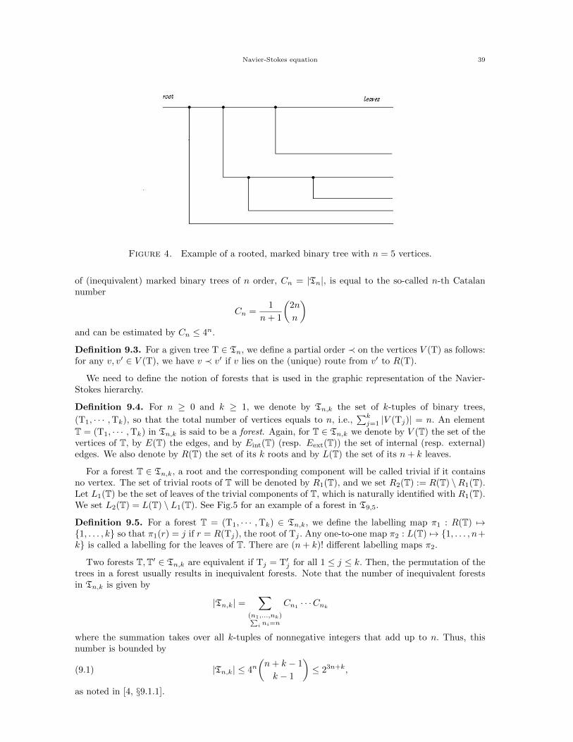
Navier-Stokes equation 39
Figure 4. Example of a rooted, marked binary tree with n = 5 vertices.
of (inequivalent) marked binary trees of n order, Cn = |Tn|, is equal to the so-called n-th Catalannumber
Cn =1
n+ 1
(2n
n
)and can be estimated by Cn ≤ 4n.
Definition 9.3. For a given tree T ∈ Tn, we define a partial order ≺ on the vertices V (T) as follows:for any v, v′ ∈ V (T), we have v ≺ v′ if v lies on the (unique) route from v′ to R(T).
We need to define the notion of forests that is used in the graphic representation of the Navier-Stokes hierarchy.
Definition 9.4. For n ≥ 0 and k ≥ 1, we denote by Tn,k the set of k-tuples of binary trees,
(T1, · · · ,Tk), so that the total number of vertices equals to n, i.e.,∑kj=1 |V (Tj)| = n. An element
T = (T1, · · · ,Tk) in Tn,k is said to be a forest. Again, for T ∈ Tn,k we denote by V (T) the set of thevertices of T, by E(T) the edges, and by Eint(T) (resp. Eext(T)) the set of internal (resp. external)edges. We also denote by R(T) the set of its k roots and by L(T) the set of its n+ k leaves.
For a forest T ∈ Tn,k, a root and the corresponding component will be called trivial if it containsno vertex. The set of trivial roots of T will be denoted by R1(T), and we set R2(T) := R(T) \R1(T).Let L1(T) be the set of leaves of the trivial components of T, which is naturally identified with R1(T).We set L2(T) = L(T) \ L1(T). See Fig.5 for an example of a forest in T9,5.
Definition 9.5. For a forest T = (T1, · · · ,Tk) ∈ Tn,k, we define the labelling map π1 : R(T) 7→{1, . . . , k} so that π1(r) = j if r = R(Tj), the root of Tj . Any one-to-one map π2 : L(T) 7→ {1, . . . , n+k} is called a labelling for the leaves of T. There are (n+ k)! different labelling maps π2.
Two forests T,T′ ∈ Tn,k are equivalent if Tj = T′j for all 1 ≤ j ≤ k. Then, the permutation of thetrees in a forest usually results in inequivalent forests. Note that the number of inequivalent forestsin Tn,k is given by
|Tn,k| =∑
(n1,...,nk)∑i ni=n
Cn1· · ·Cnk
where the summation takes over all k-tuples of nonnegative integers that add up to n. Thus, thisnumber is bounded by
(9.1) |Tn,k| ≤ 4n(n+ k − 1
k − 1
)≤ 23n+k,
as noted in [4, §9.1.1].
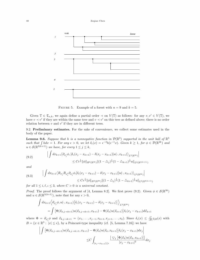
40 Zeqian Chen
Figure 5. Example of a forest with n = 9 and k = 5.
Given T ∈ Tn,k, we again define a partial order ≺ on V (T) as follows: for any v, v′ ∈ V (T), wehave v ≺ v′ if they are within the same tree and v ≺ v′ on this tree as defined above; there is no orderrelation between v and v′ if they are in different trees.
9.2. Preliminary estimates. For the sake of convenience, we collect some estimates used in thebody of the paper.
Lemma 9.6. Suppose that h is a nonnegative function in D(R3) supported in the unit ball of R3
such that∫hdx = 1. For any ε > 0, we let δε(x) = ε−3h(ε−1x). Given k ≥ 1, for φ ∈ D(R3k) and
u ∈ S(R3(k+1)) we have, for every 1 ≤ j ≤ k,∣∣∣ ∫ dxk+1
⟨∂xijφ, [δε(xj − xk+1)− δ(xj − xk+1)]u(·, xk+1)
⟩L2(R3k)
∣∣∣≤ Cε 1
2 ‖φ‖H2(R3k)‖(1−4j)12 (1−4k+1)
12u‖L2(R3(k+1))
(9.2)
and ∣∣∣ ∫ dxk+1
⟨RxιjRx`j∂xijφ,[δε(xj − xk+1)− δ(xj − xk+1)]u(·, xk+1)
⟩L2(R3k)
∣∣∣≤ Cε 1
2 ‖φ‖H2(R3k)‖(1−4j)12 (1−4k+1)
12u‖L2(R3(k+1))
(9.3)
for all 1 ≤ i, `, ι ≤ 3, where C > 0 is a universal constant.
Proof. The proof follows the argument of [4, Lemma 8.2]. We first prove (9.2). Given φ ∈ S(R3k)and u ∈ S(R3(k+1)), note that for any ε > 0,∫
dxk+1
⟨∂xijφ, u(·, xk+1)
[δε(xj − xk+1)− δ(xj − xk+1)
]⟩L2(R3k)
=
∫ [Φ(~xk,j→k+1)u(~xk,j→k+1, xk+1)− Φ(~xk)u(~xk+1)
]δε(xj − xk+1)d~xk+1
where Φ = ∂xijφ and ~xk,j→k+1 = (x1, . . . , xj−1, xk+1, xj+1, . . . , xk). Since δε(x) ≤ C|B|χB(x) with
B = {x ∈ R3 : |x| ≤ ε}, by a Poincare-type inequality (cf. [5, Lemma 7.16]) we have∣∣∣∣ ∫ [Φ(~xk,j→k+1)u(~xk,j→k+1, xk+1)− Φ(~xk)u(~xk, xk+1)]δε(xj − xk+1)dxj
∣∣∣∣≤C
∫|xj−xk+1|≤ε
∣∣5j [Φ(~xk)u(~xk, xk+1)]∣∣
|xj − xk+1|2dxj

Navier-Stokes equation 41
for all ~xk,j→k+1, where C is a universal constant. Inserting this inequality on the right hand side ofthe proceeding equality and applying the Schwarz inequality, we have∣∣∣∣ ∫ dxk+1
⟨∂xijφ, u(·, xk+1)
[δε(xj − xk+1)− δ(xj − xk+1)
]⟩L2(R3k)
∣∣∣∣.∫ [| 5j Φ(~xk)||u(~xk+1)|+ |Φ(~xk)|| 5j u(~xk+1)|
]χ{|xj−xk+1|≤ε}(~xk+1)d~xk+1
|xj − xk+1|2
.
(∫| 5j Φ(~xk)|2
χ{|xj−xk+1|≤ε}(~xk+1)d~xk+1
|xj − xk+1|2
) 12(∫
|u(~xk+1)|2χ{|xj−xk+1|≤ε}(~xk+1)d~xk+1
|xj − xk+1|2
) 12
+
(∫|Φ(~xk)|2
χ{|xj−xk+1|≤ε}(~xk+1)d~xk+1
|xj − xk+1|2
) 12(∫
| 5j u(~xk+1)|2χ{|xj−xk+1|≤ε}(~xk+1)d~xk+1
|xj − xk+1|2
) 12
.
In the terms containing Φ we perform the xk+1 integration and obtain(∫χ{|xj−xk+1|≤ε}(~xk+1)
|xj − xk+1|2| 5j Φ(~xk)|2d~xk+1
) 12
≤ ε 12 ‖φ‖H2(R3k)
and (∫χ{|xj−xk+1|≤ε}(~xk+1)
|xj − xk+1|2|Φ(~xk)|2d~xk+1
) 12
≤ ε 12 ‖φ‖H1(R3k).
In the terms containing u, dropping the restriction χ{|xj−xk+1|≤ε} and applying the Hardy inequalityto the xk+1-integration, we obtain(∫
χ{|xj−xk+1|≤ε}(~xk+1)
|xj − xk+1|2|u(~xk+1)|2d~xk+1
) 12
≤(∫
| 5k+1 u(~xk+1)|2d~xk+1
) 12
≤ ‖(1−4j)12 (1−4k+1)
12u‖L2(R3(k+1))
and (∫χ{|xj−xk+1|≤ε}(~xk+1)
|xj − xk+1|2| 5j u(~xk+1)|2d~xk+1
) 12
≤(∫
| 5j 5k+1u(~xk+1)|2d~xk+1
) 12
≤ ‖(1−4j)12 (1−4k+1)
12u‖L2(R3(k+1)).
In summary, we get the inequality (9.2).Thanks to the fact that Riesz transforms Rxi are bounded on L2(R3), replacing φ by RxιjRx`jφ in
(9.2) we obtain (9.3). �
Lemma 9.7. (cf. [4, Lemma A.3]) Let V be a nonnegative function in L1(R3). Then there exists auniversal constant C > 0 such that∫
dxdyV (x− y)|u(x, y)|2 ≤ C‖V ‖1‖u‖2H1(2)
for all u ∈ H1(2)(R
3).
Lemma 9.8. (cf. [4, Lemma 10.1]) For three nonnegative numbers ε, λ, η satisfying 0 ≤ ε < λ < 1and 0 < η < λ− ε, there exists a constant Cε,λ,η > 0 such that∫ ∞
−∞
dβ
〈α− β〉1−ε|β|λ≤ Cε,λ,η
1
〈α〉λ−ε−η
for all α ∈ R.
Lemma 9.9. For three nonnegative numbers ε, λ, η satisfying 0 ≤ ε < λ < 1 and 0 < η < λ− ε, thereexists a constant Cε,λ,η > 0 such that∫ ∞
−∞
dt
|s− t+ ai|1−ε|t+ bi|λ≤ Cε,λ,η
1
|s+ (a+ b)i|λ−ε−η
for all a, b ≥ 1 and s ∈ R.
42 Zeqian Chen
Proof. Without loss of generality, we can assume that a ≥ b ≥ 1. By Lemma 9.8, we have∫ ∞−∞
dt
|s− t+ ai|1−ε|t+ bi|λ=
1
aλ−ε
∫ ∞−∞
dt
|s/a− t+ i|1−ε|t+ ib/a|λ
≤ 1
aλ−ε
∫ ∞−∞
dt
〈s/a− t〉|t|λ≤ Cε,λ,η
1
|s+ (a+ b)i|λ−ε−η
where we use in the last inequality the conditions a ≥ b ≥ 1 and η ≥ 0. �
Acknowledgment. The author is grateful to Chuangye Liu for making helpful suggestions on thedraft of the manuscript. This work was partially supported by the Natural Science Foundation ofChina under Grant No.11431011.
References
[1] Z. Chen, Local well-posedness for Gross-Pitaevskii hierarchies, Acta Anal. Funct. Appl. 15 (2013), 291-305.
[2] N. Dunford, J. T. Schwartz, Linear Operators, Part I: General Theory, Interscience Publishers, INC., New York,
1964.[3] J. Diestel, J.J. Uhl,Jr., Vector Measures, American Mathematical Society, Providence, Rhode Island, 1977.
[4] L. Erdos, B. Schlein, H. T. Yau, Derivation of the cubic non-linear Schrodinger equation from quantum dynamics
of many-body systems, Invent. Math. 167 (2007), 515-614.[5] D. Gilbarg, N. S. Trudinger, Elliptic Partial Differential Equations of Second Order (Second edition), Springer-
Verlag, Berlin, 2001.
[6] J. Leray, Sur le mouvement d’un fluide visqueux emplissant l’espace, Acta Math. 63 (1934), 193-248.[7] P. G. Lemarie-Rieusset, Recent Developments in the Navier-Stokes Problem, Chapman & Hall/CRC, Boca Raton,
2002.[8] P. G. Lemarie-Rieusset, The Navier-Stokes Problem in the 21st Century, CRC Press, Boca Raton, 2016.
Wuhan Institute of Physics and Mathematics, Chinese Academy of Sciences, 30 West District, Xiao-
Hong-Shan, Wuhan 430071, China