navigating marine electromagnetic transmitters using dipole...
TRANSCRIPT
Geophysical Prospecting doi: 10.1111/1365-2478.12092
Navigating marine electromagnetic transmitters using dipole fieldgeometry
Karen Weitemeyer1∗ and Steve Constable2
1Now at University of Southampton, National Oceanography Centre, Southampton, UK, and 2Scripps Institution of Oceanography, La Jolla,CA, USA
Received November 2012, revision accepted August 2013
ABSTRACTThe marine controlled source electromagnetic (CSEM) technique has been adopted bythe hydrocarbon industry to characterize the resistivity of targets identified from seis-mic data prior to drilling. Over the years, marine controlled source electromagnetichas matured to the point that four-dimensional or time lapse surveys and monitoringcould be applied to hydrocarbon reservoirs in production, or to monitor the seques-tration of carbon dioxide. Marine controlled source electromagnetic surveys havealso been used to target shallow resistors such as gas hydrates. These novel uses ofthe technique require very well constrained transmitter and receiver geometry in orderto make meaningful and accurate geologic interpretations of the data. Current nav-igation in marine controlled source electromagnetic surveys utilize a long base line,or a short base line, acoustic navigation system to locate the transmitter and seafloorreceivers. If these systems fail, then rudimentary navigation is possible by assumingthe transmitter follows in the ship’s track. However, these navigational assumptionsare insufficient to capture the detailed orientation and position of the transmitterrequired for both shallow targets and repeat surveys. In circumstances when acousticnavigation systems fail we propose the use of an inversion algorithm that solves fortransmitter geometry. This algorithm utilizes the transmitter’s electromagnetic dipoleradiation pattern as recorded by stationary, close range (<1000 m), receivers in orderto model the geometry of the transmitter. We test the code with a synthetic model andvalidate it with data from a well navigated controlled source electromagnetic surveyover the Scarborough gas field in Australia.
Key words: Electromagnetics, Modelling.
1 INTRODUCT I ON
The marine controlled source electromagnetic (CSEM)method is becoming an integral part of hydrocarbon ex-ploration (Constable & Srnka 2007; Constable 2010), hav-ing successfully been used to distinguish water-oil con-tacts (Ellingsrud et al. 2002), estimate hydrocarbon volumes(Hoversten et al. 2006), image gas hydrates (Weitemeyer et al.2006), and proposed for use in time-lapse surveys to monitor
∗E-mail: [email protected]
the production of reservoirs and sequestration of carbon diox-ide (Orange et al. 2009; Lien & Mannseth 2008). Non-repeatability of time-lapse surveys will be dominated by thesource navigation (Zach et al. 2009), and so precise knowl-edge of the transmitter and receiver geometries is necessaryto give accurate reservoir volume estimates. Current marineCSEM surveys consist of a deep-towed transmitter (the source)and autonomous ocean bottom electromagnetic (OBEM) re-ceivers, both navigated using acoustic systems. These includeshort-base-line (SBL), ultra short base-line (USBL), and long-base-line (LBL) geometries. For transmitter navigation, both
C© 2014 European Association of Geoscientists & Engineers 1
2 K. Weitemeyer and S. Constable
CR
IPP
S I N
ST
ITUTION OF OCEANOG
RA
PHY
UCSD
EM Transmitter Deployed Ex,y,z Bx,y Receivers
Starboard iLBL
Port iLBLShip’s acousticsystem Transmitter Benthos
acoustic system
Transmitter acoustictransponder
Tail buoy; depth andacoustic transponder
Transmitter: depth, current, temperature, pitch, roll, heading, altitude, sound velocity, conductivity
OBEM with acoustic transponders
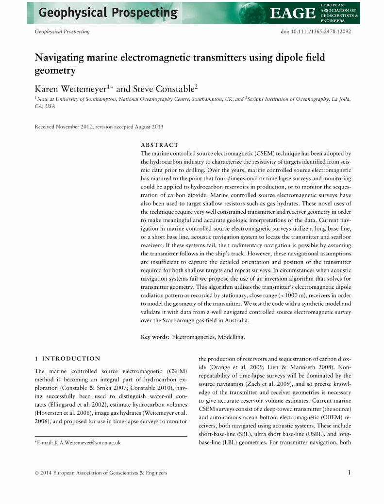
Figure 1 Example of an inverted long baseline (iLBL) acoustic navigation system employed during the Scarborough gas field CSEM survey in2009.
LBL and USBL systems can be configured in an invertedmode, ranging from the transmitter rather than the vessel.Inverted USBL systems (iUSBL) range from the transmitterto locate the far end of the antenna. Inverted long baseline(iLBL) acoustic navigation systems range from the transmit-ter to transponders on sea floor instruments or transpondersattached to paravanes towed behind the survey vessel to solvefor transmitter position (Key and Constable, 2011; Figure 1).A relay transponder on the far end of the antenna can beused to obtain antenna geometry. The source navigation ac-curacy depends on water depth, but commercial surveyorsreport that the source location is given to within a few metersin the horizontal position, 10 cm in vertical altitude abovethe seafloor and less than 1 degree for the source dipole ori-entation (Zach et al. 2009). These values may be achievedin ideal circumstances, but in practice transmitter navigationerrors can be much larger (Constable 2013). Should theseacoustic navigation systems fail, as happened in our 2004Hydrate Ridge and the 2008 Gulf of Mexico CSEM exper-iments, we can use an inverse method to determine sourceorientation by utilizing the near-field electromagnetic (EM)radiation pattern of the electric dipole source. Near field (inthis case <1 km in source-receiver offset) electric and mag-netic data collected by seafloor receivers are less sensitive toseafloor resistivity than far field (>1 km) data, and can beused to refine the geometry of the transmitter and receivers,since the CSEM signal recorded at receivers will be dominatedby energy propagating directly through the highly conductingwater (Lien & Mannseth 2008). We choose to distinguishnear and far field at a range of 1000 m based on where the
rate of decay of the electric field amplitudes changes, whichis associated with the a transition from geometric spreadingto a more dominant inductive influence from the seafloorresistivity. We note, however, that seafloor resistivity has agalvanic influence at all ranges, causing the electric field am-plitudes to be higher the more resistive the seafloor. Sincenavigational effects dominate in the near field this makes thenear field region useful for determining transmitter geome-try. Swidinsky & Edwards (2011) have proposed the use ofan eigenparameter statistical analysis as a substitute to SBLsystems for solving the x and y position of a towed receiverarray simultaneously with a 1D layered seafloor resistivity.Here we propose the use of a Levenberg-Marquardt and/orOccam inversion scheme to solve for navigational parametersincluding transmitter position (x, y), heading (θ ), dip (φ), andhalf-space resistivity below the transmitter (ρ) as well as re-ceiver positions (x, y) when acoustic navigation systems failor navigational accuracy is insufficient for the intended useof the data. The inversion program described here uses theone dimensional dipole forward modeling code, Dipole1D,of Key (2009) and requires an initial estimate of half-spaceseafloor resistivity and an initial geometry for the transmitterand receivers. The program updates the model parameters un-til convergence is reached between the synthetic EM responsesand the observed EM data. We call this technique “total fieldnavigation” (TFN) and applied it to a synthetic model, awell navigated CSEM data set collected from Scarboroughgas field in Australia (2009), and the poorly navigated Gulf ofMexico gas hydrate (2008) and Hydrate Ridge (2004) CSEMsurveys.
C© 2014 European Association of Geoscientists & Engineers, Geophysical Prospecting, 1–24
Transmitter navigation in marine electromagnetic surveys 3
2 T HE ELECTRIC D IPOLE FIELD
The mathematical description of the horizontal electromag-netic dipole (HED) source can be found in Chave & Cox(1982) and in Ward & Hohmann (1987). The 1D CSEM for-ward modeling Fortran code, Dipole1D, used in this studywas developed by Key (2009) and uses a Lorentz gauged vec-tor potential formulation of Maxwell’s equations and digitalfilter coefficients of Kong (2007) for the Hankel transforms.The source dipole can be modeled either as a point sourcedipole or a finite length source dipole; for our purposes weuse a finite dipole and we refer the reader to Streich & Becken(2010) for a discussion on the importance of accurately rep-resenting the source length. Unlike the code of Flosadottir &Constable (1996), Dipole1D is capable of computing the EMfields from an arbitrarily oriented electric dipole transmitter,essential for this application.
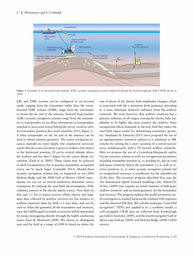
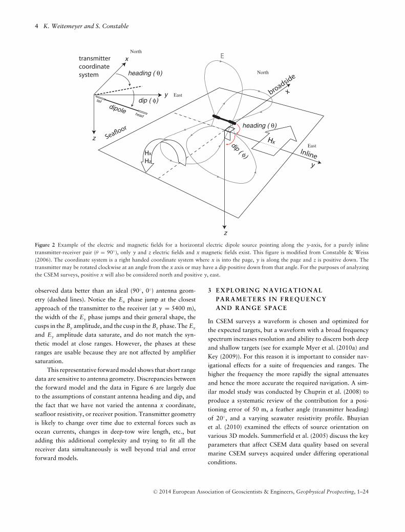
The Dipole1D code used for all modeling in the paperuses a right-handed Cartesian coordinate system (x, y, z),rather than a cylindrical coordinate system, allowing directcomparison of model response with field data without theneed of a coordinate transformation. Figure 2 outlines thegeometry considered: transmitter heading or azimuth (θ ) isthe angle from the x-axis to the antenna in the horizontalplane, and transmitter dip (φ) is the antenna angle betweenthe horizontal plane and the antenna. Note that the defi-nition of azimuth from Constable & Cox (1996) refers tothe angle between the transmitter antenna and the receiv-ing antenna, yet commonly azimuth is also used as the an-gle from the antenna to North. To avoid confusion betweenthese two definitions we will use the term heading for thelatter.
We can compute the dipole geometry for increasinglycomplicated transmitter orientations. We first consider amodel consisting of a 1 �m seafloor with seawater resistivityof 0.3 �m and a grid of transmitter positions, 100 m above asingle receiver placed on the seafloor at the center of the grid.The grid of transmitters have the same 90◦ heading and 0◦ dipthroughout the model (Figure 3).
Note this is not quite the same as the fields emanatingfrom a single transmitter located above the seafloor – by reci-procity it is equivalent to fields at 100 m altitude emanatingfrom a seafloor transmitter. Phase jumps and decreases in am-plitude are common in the Ex, Ez, and By field componentswhen the transmitter crosses the axis of the receiver. The signof the 180◦ phase jump in Ex and By is dependent on whetherthe transmitter is on the north (+x) or south (−x) side of thereceiver, an important indicator for transmitter location unre-
solved with in-line data (Ey, Ez, and Bx) alone (here we haveused the phase lead convention; phases become increasinglynegative with source-receiver offset). The Ez component hasa single 180◦ phase jump resulting from the change in sign ofthe dipole field lines. The in-line Ey has two 90◦ phase jumpsthat are symmetric about the x axis and whose distance de-pends on the separation of the transmitter and receiver alongx. The Ey phase is 180◦ where the transmitter is 100 m di-rectly above the receiver because Ey is associated with a returncurrent there.
In practice, very close range transmitter positions can sat-urate the receiver amplifiers unless some type of gain-rangingor multi-gain system is used. Some contractor instrumentsemploy these schemes, but, as we have indicated, short-rangedata have limited sensitivity to seafloor resistivity and are notrequired for routine CSEM interpretations. However, satura-tion of the electric field amplifiers eliminates the close-rangefeatures in electric field amplitude for constraining the dip andheading of the transmitter. In field data where By and Bx donot saturate at close range the cusps in amplitude can be usedto constrain the orientation and position of the transmitterand receivers.
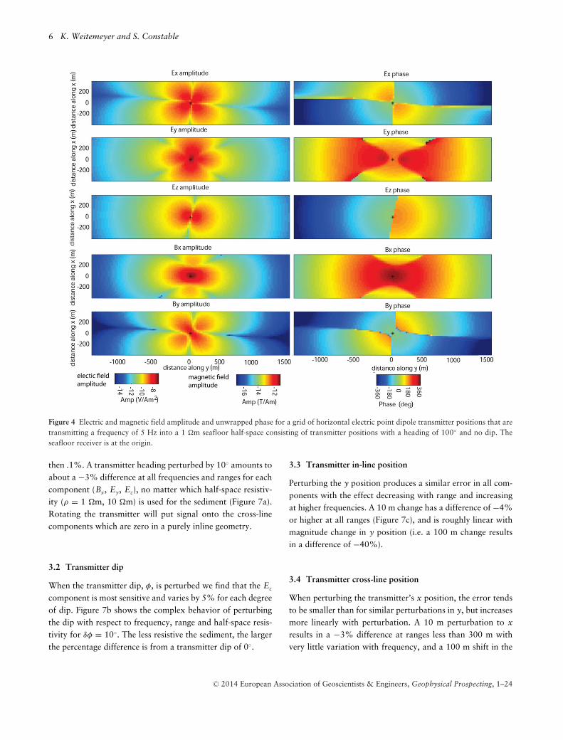
Having examined the general features for purely y-oriented transmitters we can examine the influence of chang-ing the heading and dip of the antenna. For example, Figure 4shows a model for a transmitter heading of 100◦ (i.e. 10◦ fromnominal), which simply rotates most of the features observedin Figure 3. The zero crossing point in the Ex and By phasesare more complex than simple rotation, with jumps in phasethat cannot be unwrapped. The zero crossing points are alsoskewed. This is important if one were to select a transmitterprofile, say, along x = 200 m.
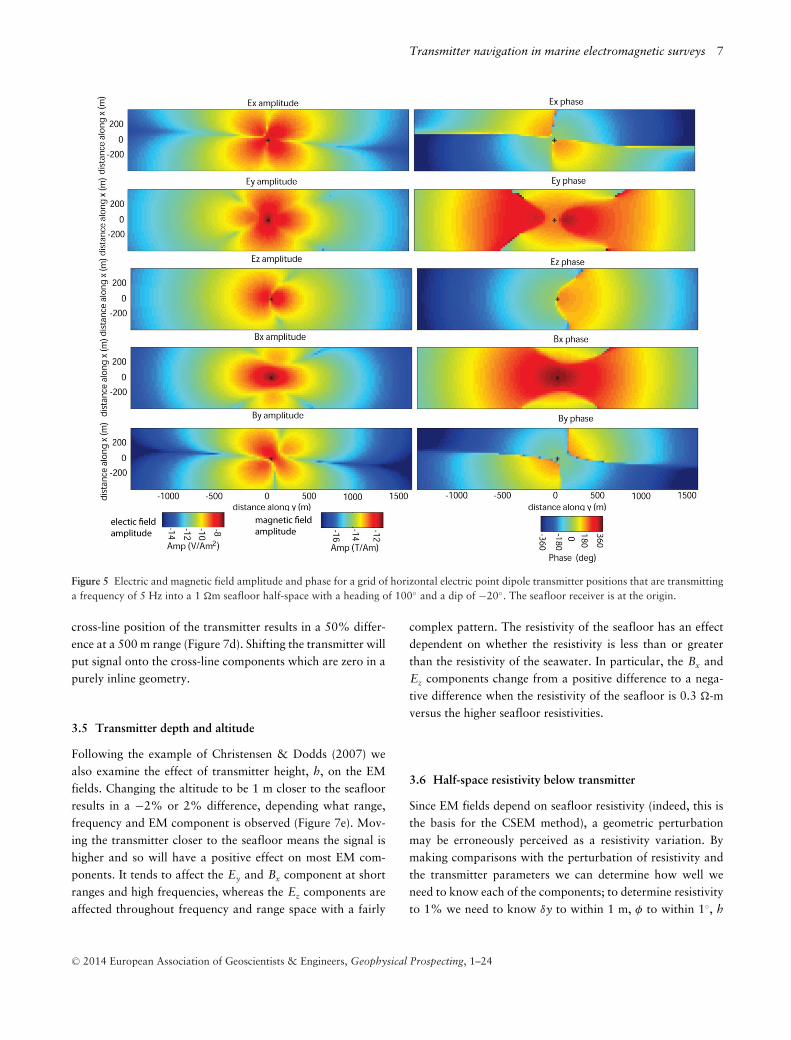
Finally, a transmitter dip of −20◦ and heading of 100◦
is shown in Figure 5. The amplitudes are no longer symmet-ric and for negative y fall off more rapidly in Ex and Ey,and more slowly in the Bx, By, and Ez components. Thisasymmetry in amplitude could easily be mistaken for geo-logic structure on the east or west side of the instrument if“ideal” antenna orientation was assumed (90◦ heading and0◦ dip). Later in section 9 we demonstrate how using poortransmitter navigation can significantly alter apparent resis-tivity pseudosections and the subsequent interpretation ofgeology.
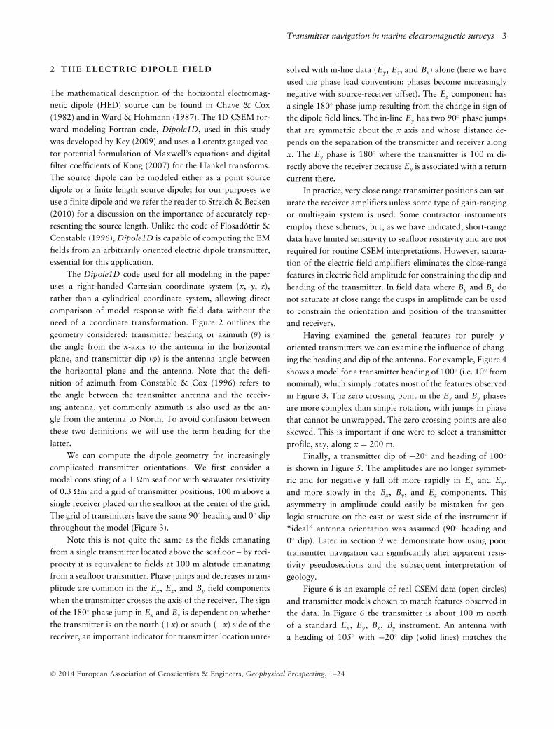
Figure 6 is an example of real CSEM data (open circles)and transmitter models chosen to match features observed inthe data. In Figure 6 the transmitter is about 100 m northof a standard Ex, Ey, Bx, By instrument. An antenna witha heading of 105◦ with −20◦ dip (solid lines) matches the
C© 2014 European Association of Geoscientists & Engineers, Geophysical Prospecting, 1–24
4 K. Weitemeyer and S. Constable
x
y
z
heading ( θ)
dip ( φ)dipole
head
tail
North
East
transmitter
coordinate
system
Inline y
broadside
x
Seafloor
z
heading ( θ)
dip ( φ)East
North
Hx
E
Hx
Hz
Figure 2 Example of the electric and magnetic fields for a horizontal electric dipole source pointing along the y-axis, for a purely inlinetransmitter-receiver pair (θ = 90◦), only y and z electric fields and x magnetic fields exist. This figure is modified from Constable & Weiss(2006). The coordinate system is a right handed coordinate system where x is into the page, y is along the page and z is positive down. Thetransmitter may be rotated clockwise at an angle from the x axis or may have a dip positive down from that angle. For the purposes of analyzingthe CSEM surveys, positive x will also be considered north and positive y, east.
observed data better than an ideal (90◦, 0◦) antenna geom-etry (dashed lines). Notice the Ex phase jump at the closestapproach of the transmitter to the receiver (at y = 5400 m),the width of the Ey phase jumps and their general shape, thecusps in the By amplitude, and the cusp in the Bx phase. The Ex
and Ey amplitude data saturate, and do not match the syn-thetic model at close ranges. However, the phases at theseranges are usable because they are not affected by amplifiersaturation.
This representative forward model shows that short rangedata are sensitive to antenna geometry. Discrepancies betweenthe forward model and the data in Figure 6 are largely dueto the assumptions of constant antenna heading and dip, andthe fact that we have not varied the antenna x coordinate,seafloor resistivity, or receiver position. Transmitter geometryis likely to change over time due to external forces such asocean currents, changes in deep-tow wire length, etc., butadding this additional complexity and trying to fit all thereceiver data simultaneously is well beyond trial and errorforward models.
3 EXPLORING NAVIGATIONALPARAMETERS IN FREQUENCYA N D R A N G E S P A C E
In CSEM surveys a waveform is chosen and optimized forthe expected targets, but a waveform with a broad frequencyspectrum increases resolution and ability to discern both deepand shallow targets (see for example Myer et al. (2010a) andKey (2009)). For this reason it is important to consider nav-igational effects for a suite of frequencies and ranges. Thehigher the frequency the more rapidly the signal attenuatesand hence the more accurate the required navigation. A sim-ilar model study was conducted by Chuprin et al. (2008) toproduce a systematic review of the contribution for a posi-tioning error of 50 m, a feather angle (transmitter heading)of 20◦, and a varying seawater resistivity profile. Bhuyianet al. (2010) examined the effects of source orientation onvarious 3D models. Summerfield et al. (2005) discuss the keyparameters that affect CSEM data quality based on severalmarine CSEM surveys acquired under differing operationalconditions.
C© 2014 European Association of Geoscientists & Engineers, Geophysical Prospecting, 1–24

Transmitter navigation in marine electromagnetic surveys 5
Figure 3 Electric and magnetic field amplitude and unwrapped phase for a grid of horizontal electric point dipole transmitter positions in planview, all at a heading of 90◦ and a dip of 0◦, for a 5 Hz transmission frequency into a 1 �m seafloor half-space. The seafloor receiver is at theorigin.
A transmitter’s position can be expressed by its northing,easting, depth below sea-surface, and altitude above the sea-floor, referred to here as x, y, z, and h. A transmitter’s ori-entation can be expressed as the heading from north (θ ) anddip from horizontal (φ) (we do not need to consider the rollof the transmitter). The resistivity of the seafloor below thetransmitter is referred to as ρ. Using Dipole1D we explore theeffect of perturbing (δ) each of these parameters as a functionof frequency and range.
For the purposes of this model study we define “stan-dard” transmitter geometry as a 50 m finite length dipoleantenna aligned along the y-axis at x = 0, y = 0–2000 m,z = 820 m, an altitude of h = 50 m with a purely in-linegeometry (transmitter heading is θ = 90◦, and dip is φ = 0◦).We model frequencies logarithmically spaced between 0.1 Hz
and 300 Hz with transmitters placed up to a range of 2000 mfrom a sea-floor receiver centered at the origin (x = 0, y =0, z = 870). We also examine different sea-floor half-spaceresistivities of ρ = 0.3, 1, and 10 �m to see if perturbations inthe navigational parameters are worse as seafloor resistivitychanges. We use percentage difference between a perturba-tion in a navigational parameter to the “standard” transmitteroutlined above to evaluate each parameter’s contribution andpresent the results in Figure 7.
3.1 Transmitter heading
We find that perturbations of 0.1◦ and 1◦ in transmitter head-ing produce a negligible effect; the percentage difference is less
C© 2014 European Association of Geoscientists & Engineers, Geophysical Prospecting, 1–24
6 K. Weitemeyer and S. Constable
Figure 4 Electric and magnetic field amplitude and unwrapped phase for a grid of horizontal electric point dipole transmitter positions that aretransmitting a frequency of 5 Hz into a 1 �m seafloor half-space consisting of transmitter positions with a heading of 100◦ and no dip. Theseafloor receiver is at the origin.
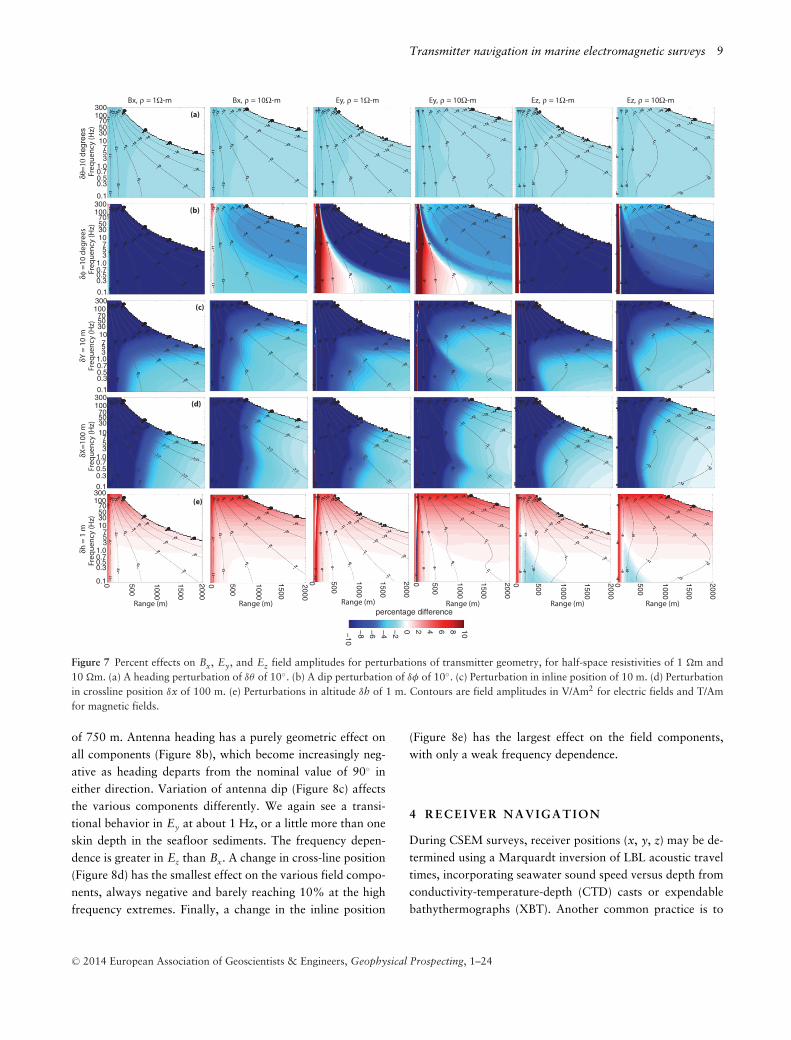
then .1%. A transmitter heading perturbed by 10◦ amounts toabout a −3% difference at all frequencies and ranges for eachcomponent (Bx, Ey, Ez), no matter which half-space resistiv-ity (ρ = 1 �m, 10 �m) is used for the sediment (Figure 7a).Rotating the transmitter will put signal onto the cross-linecomponents which are zero in a purely inline geometry.
3.2 Transmitter dip
When the transmitter dip, φ, is perturbed we find that the Ez
component is most sensitive and varies by 5% for each degreeof dip. Figure 7b shows the complex behavior of perturbingthe dip with respect to frequency, range and half-space resis-tivity for δφ = 10◦. The less resistive the sediment, the largerthe percentage difference is from a transmitter dip of 0◦.
3.3 Transmitter in-line position
Perturbing the y position produces a similar error in all com-ponents with the effect decreasing with range and increasingat higher frequencies. A 10 m change has a difference of −4%or higher at all ranges (Figure 7c), and is roughly linear withmagnitude change in y position (i.e. a 100 m change resultsin a difference of −40%).
3.4 Transmitter cross-line position
When perturbing the transmitter’s x position, the error tendsto be smaller than for similar perturbations in y, but increasesmore linearly with perturbation. A 10 m perturbation to x
results in a −3% difference at ranges less than 300 m withvery little variation with frequency, and a 100 m shift in the
C© 2014 European Association of Geoscientists & Engineers, Geophysical Prospecting, 1–24
Transmitter navigation in marine electromagnetic surveys 7
Figure 5 Electric and magnetic field amplitude and phase for a grid of horizontal electric point dipole transmitter positions that are transmittinga frequency of 5 Hz into a 1 �m seafloor half-space with a heading of 100◦ and a dip of −20◦. The seafloor receiver is at the origin.
cross-line position of the transmitter results in a 50% differ-ence at a 500 m range (Figure 7d). Shifting the transmitter willput signal onto the cross-line components which are zero in apurely inline geometry.
3.5 Transmitter depth and altitude
Following the example of Christensen & Dodds (2007) wealso examine the effect of transmitter height, h, on the EMfields. Changing the altitude to be 1 m closer to the seafloorresults in a −2% or 2% difference, depending what range,frequency and EM component is observed (Figure 7e). Mov-ing the transmitter closer to the seafloor means the signal ishigher and so will have a positive effect on most EM com-ponents. It tends to affect the Ey and Bx component at shortranges and high frequencies, whereas the Ez components areaffected throughout frequency and range space with a fairly
complex pattern. The resistivity of the seafloor has an effectdependent on whether the resistivity is less than or greaterthan the resistivity of the seawater. In particular, the Bx andEz components change from a positive difference to a nega-tive difference when the resistivity of the seafloor is 0.3 �-mversus the higher seafloor resistivities.
3.6 Half-space resistivity below transmitter
Since EM fields depend on seafloor resistivity (indeed, this isthe basis for the CSEM method), a geometric perturbationmay be erroneously perceived as a resistivity variation. Bymaking comparisons with the perturbation of resistivity andthe transmitter parameters we can determine how well weneed to know each of the components; to determine resistivityto 1% we need to know δy to within 1 m, φ to within 1◦, h
C© 2014 European Association of Geoscientists & Engineers, Geophysical Prospecting, 1–24

8 K. Weitemeyer and S. Constable
4000 4500 5000 5500 6000 6500-14
-12
-10
-8
4000 4500 5000 5500 6000 6500-400
-200
0
200Ex
4000 4500 5000 5500 6000 6500-40
60
160
260
360
Ey
4000 4500 5000 5500 6000 6500-18
-16
-14
-12
4000 4500 5000 5500 6000 6500-400
-200
0
200By
4000 4500 5000 5500 6000 6500-17
-16
-15
-14
-13
-12
4000 4500 5000 5500 6000 6500-500
-400
-300
-200
-100
0
Ex
Bx
4000 4500 5000 5500 6000 6500-14
-12
-10
-8
Pha
se (
degr
ees)
Pha
se (
degr
ees)
Pha
se (
degr
ees)
Pha
se (
degr
ees)
PHASEAMPLITUDEM
agne
tic F
ield
Am
plitu
de
(T
/Am
)M
agne
tic F
ield
Am
plitu
de
(T
/Am
)E
lect
ric F
ield
Am
plitu
de
(V
/Am
)
2E
lect
ric F
ield
Am
plitu
de
(V
/Am
)
2
distance along y (m) distance along y (m)
Bx
By
Ey
Tx-Rot 90,Tx-dip 0
Tx-Rot 105,Tx-dip -20s22 data x-coordinates22 data y-coordinate
Figure 6 Example of the 2004 Hydrate Ridge field data compared to a 1D forward model of electric and magnetic fields for a transmitterheading of 105◦ and a dip of −20◦ at receiver site 22 (solid line). The dashed line is for a horizontal transmitter with a heading of 90◦. Electricfield amplitudes saturate at about 10−10 V/Am2 (left panel). Unwrapped phases are plotted in the right panel. Open circles are the field data.The arrows show where transmitter heading and dip are affecting the EM data. The blue triangle indicates seafloor receiver location.
to within 1 m, θ to within 10◦, and δx to within 10 m. Thispattern scales linearly.
3.7 Perturbations of transmitter geometry at a fixed range
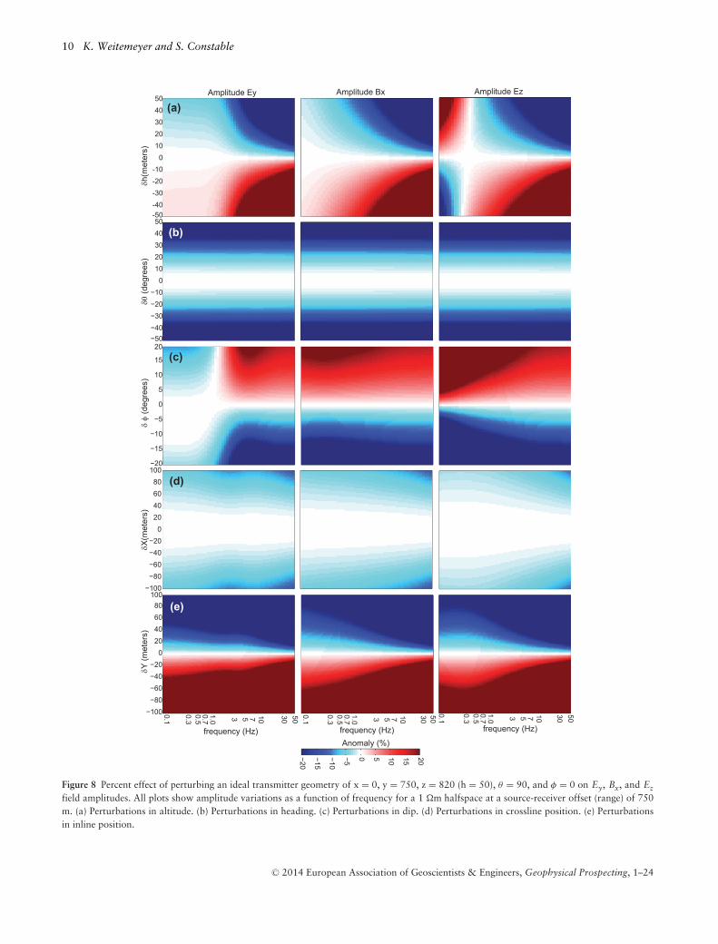
In Figure 8 we examine the variations in field component am-plitudes as a function of frequency due to perturbations intransmitter geometry at a fixed source receiver offset (range)of 750 m. Changes in altitude (Figure 8a) result in positivechanges to all components when the transmitter is lowered
from its nominal 50 m altitude, and negative changes whenthe transmitter altitude is increased. The exception is the lowfrequency Ez amplitudes, which produce an anti-symmetricpattern about 0.3 Hz. The low frequency Ez behavior maybe understood by considering a static dipole field – as onegets closer to the dipole axis the vertical component goes to-wards zero. The high frequency behavior is interpreted as aninductive phenomenon similar to the Ey and Bx components.The transition frequency of 0.3 Hz corresponds to a little morethan one skin depth in seawater over the source-receiver range
C© 2014 European Association of Geoscientists & Engineers, Geophysical Prospecting, 1–24
Transmitter navigation in marine electromagnetic surveys 9
0.1
0.30.50.71.0
357
10305070
100300
Fre
qu
en
cy (
Hz)
Bx, ρ = 1Ω-m Bx, ρ = 10Ω-m Ey, ρ = 1Ω-m Ey, ρ = 10Ω-m Ez, ρ = 1Ω-m Ez, ρ = 10Ω-m
δθ=1
0 degrees
0.30.50.71.0
357
10305070
100300
Fre
qu
en
cy (
Hz)
δφ =
10
de
gre
es
−11
0.1
0.30.50.71.0
357
10305070
100300
Fre
qu
en
cy (
Hz)
δY =
10
m
0.1
0.30.50.71.0
357
10305070
100300
Fre
qu
en
cy (
Hz)
δX=
10
0 m
0 500
1000
1500
2000
percentage difference
−10
−8
−6
−4
−2
0 2 4 6 8 10
0 500
1000
1500
2000
0 500
1000
1500
2000
0 500
1000
1500
2000
0 500
1000
1500
2000
500
1000
1500
2000
00.1
0.30.50.71.0
357
10305070
100300
Fre
qu
en
cy (
Hz)
δh =
1 m
Range (m) Range (m) Range (m) Range (m) Range (m) Range (m)
(a)
(b)
(c)
(d)
(e)
0.1
Figure 7 Percent effects on Bx, Ey, and Ez field amplitudes for perturbations of transmitter geometry, for half-space resistivities of 1 �m and10 �m. (a) A heading perturbation of δθ of 10◦. (b) A dip perturbation of δφ of 10◦. (c) Perturbation in inline position of 10 m. (d) Perturbationin crossline position δx of 100 m. (e) Perturbations in altitude δh of 1 m. Contours are field amplitudes in V/Am2 for electric fields and T/Amfor magnetic fields.
of 750 m. Antenna heading has a purely geometric effect onall components (Figure 8b), which become increasingly neg-ative as heading departs from the nominal value of 90◦ ineither direction. Variation of antenna dip (Figure 8c) affectsthe various components differently. We again see a transi-tional behavior in Ey at about 1 Hz, or a little more than oneskin depth in the seafloor sediments. The frequency depen-dence is greater in Ez than Bx. A change in cross-line position(Figure 8d) has the smallest effect on the various field compo-nents, always negative and barely reaching 10% at the highfrequency extremes. Finally, a change in the inline position
(Figure 8e) has the largest effect on the field components,with only a weak frequency dependence.
4 R ECEIVER NAVIGATION
During CSEM surveys, receiver positions (x, y, z) may be de-termined using a Marquardt inversion of LBL acoustic traveltimes, incorporating seawater sound speed versus depth fromconductivity-temperature-depth (CTD) casts or expendablebathythermographs (XBT). Another common practice is to
C© 2014 European Association of Geoscientists & Engineers, Geophysical Prospecting, 1–24
10 K. Weitemeyer and S. Constable
Amplitude Ez
Anomaly (%)
−20
−15
−10
−5 0 5 10 15 20
Amplitude Bx
-50-40-30-20-10
01020304050
Amplitude Ey
δh(m
eter
s)
−50−40−30−20−10
01020304050
δθ
(deg
rees
)
−20
−15
−10
−5
0
5
10
15
20
δ φ
(deg
rees
)
−100−80−60−40−20
020406080
100
δX
(met
ers)
frequency (Hz)
frequency (Hz)
−100−80−60−40−20
020406080
100
frequency (Hz)
δY
(met
ers)
0.30.50.71.0 3 5 7 10 30 500.1
0.30.50.71.0 3 5 7 10 30 500.1
0.30.50.71.0 3 5 7 10 30 500.1
(a)
(b)
(c)
(d)
(e)
Figure 8 Percent effect of perturbing an ideal transmitter geometry of x = 0, y = 750, z = 820 (h = 50), θ = 90, and φ = 0 on Ey, Bx, and Ez
field amplitudes. All plots show amplitude variations as a function of frequency for a 1 �m halfspace at a source-receiver offset (range) of 750m. (a) Perturbations in altitude. (b) Perturbations in heading. (c) Perturbations in dip. (d) Perturbations in crossline position. (e) Perturbationsin inline position.
C© 2014 European Association of Geoscientists & Engineers, Geophysical Prospecting, 1–24
Transmitter navigation in marine electromagnetic surveys 11
use USBL transponders on each instrument to locate receiverson the seafloor. Since the receivers are usually dropped fromthe ship they will have an arbitrary orientation when theyarrive on the seafloor. An external compass with an internaltilt-meter may be used to measure magnetic north, instrumenttilt, and instrument pitch. In lieu of a compass, the orienta-tion may be found by utilizing the electric and magnetic phasedata at intermediate offsets from the transmitter by rotatinginstruments so the cross line component goes to a minimum(Mittet et al. 2007). Another technique uses orthogonal Pro-crustes rotation analysis (OPRA) to estimate the full 3D re-ceiver orientation for in-line and cross-line CSEM receivers(Key & Lookwood 2010). Polarization ellipses can also beused to determine receiver orientation (see Summerfield et al.(2005), Martinez et al. (2010), Weitemeyer (2008), Behrens(2005)). Zach et al. (2009) claims that the greatest acquisitionuncertainty is related to the receiver orientation, which mayhave uncertainties of up to 3-5◦ in rotation and tilt. To recovertransmitter navigation we must assume the receiver positionand orientation are known. For the Scarborough CSEM ex-periment Myer et al. (2012) estimated an upper bound on theerror in receiver orientation by comparing the measured ex-ternal compass readings to the OPRA method and found thestandard deviation of the difference to be 3.3◦, which for in-line field components equates to less than 0.35% uncertainty.Errors in receiver location estimated from Marquardt inver-sion of LBL acoustic travel times are typically 7 m horizontallyand 2 m vertically.
5 T R A N S M I T T E R NA V I G A T I O N
Transmitter navigation data recorded during deep-towingusually includes altitude (h) and pressure (which can be con-verted into a depth, z). Acoustic systems are used to computethe transmitter’s x, and y position, and in some cases one cancompute the heading, θ , of the transmitter antenna by placingan acoustic transponder at the tail. The dip φ of the antennamay be computed using two pressure gauges at the head andtail-end of the antenna or may also be computed from a sec-ond transponder. Acoustic transponders placed along the en-tire length of the antenna could be used to estimate the fullgeometry of the antenna. When acoustic navigation systemsfail, then a first order approximation is that the transmitterfollows directly in the path of the ship at a horizontal distancecomputed from the transmitter depth and the acoustic slantrange or wire out (distance from the ship to the transmitter,Figure 9). This distance changes with depth and ship’s speed.The dip of the antenna may also vary because the transmitter
is pulled in or let out to maintain a constant towing altitudeover seafloor bathymetry, or because the antenna is not per-fectly neutrally buoyant.
It is important to note that acoustic navigation only lo-cates an acoustic transponder and most sensors are attachedto the transmitter head rather than the antenna. However, itis the geometry at the center of the antenna that is requiredfor accurate modeling of the electromagnetic fields. For anacoustic transponder on the head of a transmitter towing a300 m antenna, one must estimate the center of the dipolealong an arc that is 150 m behind the head. This may be ap-proximated by projecting back the position to the center ofthe antenna by using the ship’s course, or the transmitter’sheading. However, there is uncertainty in this approximationwhich grows as the length of the antenna increase. In thesecases, some refinement to the position and orientation at thecentre of the antenna is possible with a total field navigationprogram.
The total field navigation method requires the use of anabsolute coordinate system (x, y, z). We keep the receiversin their original orientation and rotate the model to that ori-entation, so as not to contaminate noise in one channel withthe other. Absolute phase of the transmitter is required. Anissue with the use of near-field data is the saturation of theelectric and magnetic field amplifiers. Fortunately, phase datafor the electric field channels are recoverable from saturatedamplitudes. The magnetic field data of our instruments do nottypically saturate. However, we found that in cases when thisdid occur the saturated magnetic field data could not be used,as the phases are unstable. The total field navigation programuses a 1D forward modeling code and so we have to assumea 1D earth structure, forcing the seafloor to be flat and al-lowing for 3D transmitter and receiver geometry relative tothe flat seafloor. We have found that including the Ez compo-nent makes the inversion unstable as this component is moresensitive to transmitter altitude and depth variations than theother EM components, which violates our 1D assumption.
Two different inversion schemes have been used to solvefor transmitter navigational parameters, a Marquardt and anOccam inversion scheme, discussed in the next two sections.
6 M A R Q U A R D T IN V E R S I O N
We have modified the Marquardt inversion technique slightlyfrom the one presented in Weitemeyer (2008). Instead of usingnodes and interpolating transmitter positions between eachnode we perform one inversion for each transmitter position;if there are 100 transmitter positions we run 100 inversions.
C© 2014 European Association of Geoscientists & Engineers, Geophysical Prospecting, 1–24

12 K. Weitemeyer and S. Constable
(Xb,Yb,T)GPS (Zs,T)
depth
distance
acoustic range or
wire out
L/2
seafloor
L
altimeterdepth
(Zt,T)(Xa,Ya,Za,θa,φa,T)Calculate
SCRI
PPS
INSTIT
UTION OF OCEANOGRAP
HY
UCSD
Mar
ine EM Lab
tail end
depth gauge receiverφ=dip
θ=heading
N(X)
b - boat
s - transmitter (SUESI)
a - antenna
t - tail
T - time
GPS - Global positioning system
E (Y)
(Z)
Figure 9 Transmitter position is modeled assuming the transmitter follows directly behind the ship and is somewhere on a horizontal arc. ForCSEM we are most concerned with the location and geometry of the centre of the transmitter’s dipole antenna as marked by the star. Sometimeswe may refer to the geometry of the transmitter which really corresponds to the geometry at the centre of the transmitter’s antenna.
The original technique also computed receiver positions andtransmitter dip, which may still be done, but it is not dis-cussed here. Collecting CSEM data without accurate receiverpositions is not commonly practiced since it is much easier tolocate a static instrument on the seafloor using either LBL orUSBL acoustic navigation than it is to locate a moving trans-mitter. The dip of the transmitter antenna can be computedfrom depth gauges on the head and tail of the antenna.
Marquardt inversion, also called ridge regression or max-imum neighborhood method, is an algorithm for the nonlinearleast-squares estimation of parameters based on an optimuminterpolation between the Taylor series expansion and gradi-ent methods (Marquardt 1963). The predicted response, d, tobe fitted to M data, d, is given by
d = (d1, d2, d3, . . . , dM) = f (x, m), (1)
where x is the measurement system or independent data vari-ables associated with the predicted response (e.g. frequency,depth, transmitter altitude, positions, etc.), and m is the vec-tor of model parameters (e.g. transmitter heading, dip, half-space apparent resistivity, etc.). The field data have errorsς=(ς1, ς2, ς3, . . . , ςM) associated with them.
The measure of how well a model m fits the data is usuallygiven by the sum-squared misfit:
χ2 =M∑
k=1
(dk − dk
ςk
)2
(2)
=M∑
k=1
1ς2
k
[dk − f (xk, m)]2. (3)
In the least squares method χ2 is minimized with respect toall the model parameters simultaneously by differentiating andsetting to zero. When the forward model response f is non-linear it can be approximated by a Taylor series expansion off around an initial model guess m0:
dk = f (xk, m0 + �m) ≈ f (xk, mo) +N∑
j=1
∂ f (xk, m0)∂mj
δmj , (4)
where
�m = (δm1, δm2, . . . , δmN), (5)
is a model parameter perturbation. This approximation for f
is substituted into Equation 3, which is then minimized withrespect to all the model parameters to give:
β = �mα, (6)
where
βi =∑ (
1ς2
k
[dk − f (xk, m0)])
∂ f (xk, m0)∂mi
, (7)
and
α j i =∑ 1
ς2k
∂ f (xk, m0)∂mj
∂ f (xk, m0)∂mi
, (8)
often called the curvature matrix.The partial derivative matrix Jk, j = ∂ f (xk, m0)/∂mj is the
Jacobian matrix relating model perturbations to variations in
C© 2014 European Association of Geoscientists & Engineers, Geophysical Prospecting, 1–24

Transmitter navigation in marine electromagnetic surveys 13
the data around a model guess m0. The Jacobian matrix inthis application is evaluated by a central difference method.
The linearization described so far is efficient in a regionclose to a minimum in χ2 but often diverges far from the so-lution (Bevington & Robinson 2003). To compensate for thisbehavior, Marquardt suggested that one increase the diagonalterms of the curvature matrix by a factor of λ (Bevington &Robinson 2003; Marquardt 1963):
α j i = α j i (1 + λ) for j = i
α j i = α j i for j �= i ;
which for small λ reduces to the solution derived from theTaylor series expansion. For large λ the diagonal terms dom-inate and the method reduces to a gradient algorithm thatchooses a path in the direction of maximum reduction in χ2
(the method of steepest descent). The gradient algorithm isrobust to nonlinearity but is very inefficient in the parabolicregion near the solution. The limitation on the Marquardtinversion is that it still requires a reasonable starting guessfor m0. However, we found that if starting parameters basedon simple layback assumptions are used the algorithm willgenerally provide a viable solution to the navigation problem.The error associated with each of the model parameters canbe computed from the error matrix, ε, the inverse of the finalcurvature matrix, α:
ε = α−1, (9)
which is then scaled by the residual variance. The final RMSmisfit is given by:
RMS =√
χ2
M, (10)
where M is the total number of data.
7 OCCAM’S IN V ER S I ON
Occam’s inversion sets out to find the simplest or smoothestpossible model that fits the observed data adequately (Con-stable et al. 1987) by penalizing roughness, the converse ofsmoothness, subject to the constraint that the solution agreeswith the measurements.
The goodness of fit is the same as for the Marquardtmethod (Equation 3), which may also be written as:
X2 = ∣∣∣∣Wd − WF[m]∣∣∣∣ , (11)
where W is the diagonal M × M matrix
W = diag{1/ς1, 1/ς2, . . . , 1/ςM}, (12)
and F[m] is an M × N matrix whose elements are computedfrom the forward problem, d = F[m].
The model vector m is composed of the various com-ponents of the transmitter geometry (e.g. transmitter x, y
positions (mx, my), transmitter heading (mθ ), transmitter dip(mφ), or half-space resistivity below the transmitter (mρ)) tobe solved for a given number of transmitter locations NT. Forexample, if there are 50 transmitters, and we want to solvethree unknown geometries (mx, my, mθ ) and half-space resis-tivity (mρ) for each transmitter this will have 50 x 4 = 200parameters.
For a one-dimensional model the roughness can be mea-sured as
R1 =N∑
i=2
(mi − mi−1)2, (13)
which can also be expressed as
R1 = ||∂m||2, (14)
where ∂ is an N × N roughness matrix made up of −1, 1,and 0’s. However, we only want to smooth adjacent values ofeach component (e.g. mx, my, mθ , or mρ) of the NT transmitterlocations, and not smooth across component types. To dothis we construct a roughness matrix consisting of severalroughness matrices. For transmitter northing (x position):
R1x=
NT∑i=2
(mxi− mxi−1
)2. (15)
For transmitter easting (y position):
R1y=
NT∑i=2
(myi− myi−1
)2, (16)
and so on for heading θ , dip φ, and half-space resistivity ρ be-low each transmitter. In this case, the minimization problemis to minimize R1 subject to the condition that the misfit X2
is equal to a given tolerance X2� based on the uncertainties.
We want to choose a X2� that is not too close to the small-
est achievable value, as for a marginal decrease in RMS wegain a significant increase in structure or roughness to themodel (Constable et al. 1987). The problem is optimized cre-ating an unconstrained functional through the use of Lagrangemultiplier, μ−1:
U = ||∂m||2 + μ−1{||Wd − WF[m]||2 − X2∗}, (17)
C© 2014 European Association of Geoscientists & Engineers, Geophysical Prospecting, 1–24
14 K. Weitemeyer and S. Constable
where we have the roughness and misfit weighted by the La-grange multiplier. The gradient of U with respect to m is setto 0 in order to solve for the m.
μ−1(WJ)TWJm − μ−1(WJ)TWd + ∂T∂m = 0, (18)
where the M × N matrix J, Jacobian matrix, is similar to thatused for Marquardt inversion. For the central differences weuse 10 m for x, y, 1◦ for φ and θ , and 0.1 �m for ρ. Themodel parameters are updated by
mk+1(μ) = [μ∂T∂ + (WJk)TWJk]
−1(WJk)TWdk, (19)
where we sweep through values of μ computing the true misfitof the model mk+1(μ)
Xk+1(μ) = ||Wd − WF[mk+1(μ)]||. (20)
After X2� is reached μ is chosen to make Xk match this exactly.
7.1 Marquardt and Occam Inversion for NavigationalParameters
The difference between the Marquardt and Occam inversionscheme is how each handles neighboring transmitter positions:the Marquardt scheme is unaware of neighboring points andthere is no feedback for the behavior of neighboring transmit-ters, whereas the Occam scheme regularizes between trans-mitter positions and is influenced by the behavior of neigh-boring points. For this reason, the final Marquardt model issmoothed to try to eliminate scatter between adjacent points.Also, with Occam an RMS is computed for the entire tow,whereas Marquardt has an RMS misfit for each transmitter.
Since we use a 1D modeling code we have to make as-sumptions about the water depth and how receivers and trans-mitters are positioned in z. A 1D seawater profile and half-space resistivity is used and the receiver depth is fixed to bean average depth for the entire tow, which is also made theseafloor depth for the model. The transmitter’s depth, z, is the1D model depth minus the actual altitude, h. To ensure thataccurate fields are modelled we also use a finite dipole ratherthen a point dipole. However, in complex bathymetric regimesthis may not always be the case and the effective dipole lengthmay in fact be shorter. This situation is beyond the scope ofthis work, where 1D assumptions are made and no 2D ef-fects are considered, although in principle the approach wedescribe could be applied using 2D modelling.
8 S YNTHETIC TESTS OF T HE ALGORITHM
A synthetic model was used to test and verify the performanceof the Marquardt and Occam total field navigation codes.We generated electric (Ex, Ey, Ez) and magnetic (Bx, By) fieldresponses at a frequency of 6.5 Hz for a 1 �m half-space anda typical seawater conductivity profile with 63 transmitterpositions (x, y, z = 806 ∼m, θ , φ = 0◦) at a 65 m altitude and4 receiver positions (x, y, z = 871) using the Dipole1D codeof Key (2009). We contaminated these responses with 10%random Gaussian noise and used these data for a synthetictest. The error structure was 10% of the amplitude with anoise floor of 10−15 V/Am2 for electric field data and 10−17
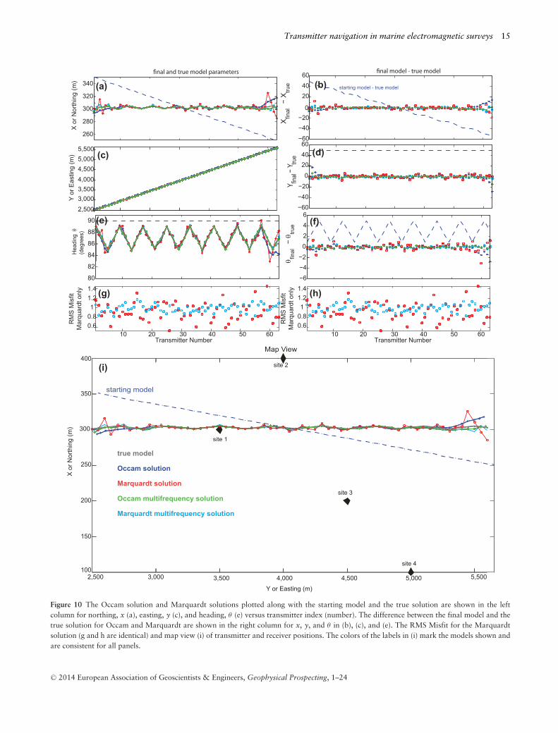
T/Am for magnetic field data. We ask the Marquardt andOccam inversion codes to solve for transmitter position andheading (m = x, y, θ ) to find the ‘true’ transmitter positions(see Figure 10 for the starting model, the true solution for thex, y, and θ of the transmitter, and a map view of the modelsand receiver locations).
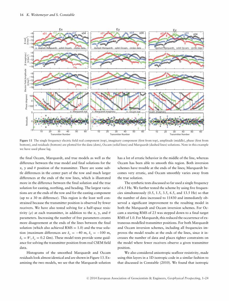
The data, d, are the real and imaginary components ofthe electric and magnetic fields at ranges <1000 m, giving atotal of 2178 data points. Real and imaginary componentsof the data are used to remove the difficulty in unwrappingphases, which can result in residuals offset by factors of 360◦.The data and fits for Marquardt and Occam are shown inFigure 11 and 12.
The Marquardt solution solves for each transmitter in-dex individually and so an RMS misfit is computed for eachtransmitter index (see Figure 10 (G and H)). In some casesthe Marquardt solution gave values that are very differentfrom neighbouring transmitters, with correspondingly highmisfits. These can be reset by using a different starting model,which in many cases allows the solution to stabilize. Some-times changing the starting halfspace resistivity is all that isrequired to give a reasonable solution. The final models aresmoothed to remove some of the scatter from the solution,and this smoothed version is used as the starting model foranother inversion. We iterate several times until the solutionmedian RMS misfit is close to 1. In this case we achieved amedian misfit of 0.91.
In the Occam inversion scheme, the starting model hadan RMS of 23 and ran to an RMS of 1.0 in 18 iterations.During the inversion, the solution initially diverges at trans-mitter numbers 20, 21, and 22, coinciding with the locationof receiver s01, where some of the the electric and magneticfields go through zero. Regularization removes this divergencein later iterations, whereas Marquardt requires some manualinput to improve the fit at these locations. Figure 10 shows
C© 2014 European Association of Geoscientists & Engineers, Geophysical Prospecting, 1–24
Transmitter navigation in marine electromagnetic surveys 15
final and true model parametersH
eadi
ng θ
(d
egre
es)
0.60.81
1.21.4
RM
S M
isfit
Mar
quar
dt o
nly (g)
100
150
200
250
300
350
400
X o
r Nor
thin
g (m
)
(i)
2,500 3,000 3,500 4,000 4,500 5,000 5,500
Y or Easting (m)
site 2
site 3
site 4
Yfin
al − Y tru
e
0.60.81
1.21.4
RM
S M
isfit
Mar
quar
dt o
nly
final model - true model
10 20 30 40 50 6010 20 30 40 50 60
(h)
Transmitter Number Transmitter Number
true model
Occam solution
Marquardt solution
Occam multifrequency solution
Marquardt multifrequency solution
starting model
site 1
Map View
−60−40
0
204060
Xfin
al −
Xtru
e
−60−40−20
0
204060
80
82
84
86
88
90
−6−4−2
0246
θfin
al −
θtru
e
−20
(b)
(d)
(f)
260
280
300
320
340
2,5003,0003,5004,0004,5005,0005,500
X o
r Nor
thin
g (m
) Y
or E
astin
g (m
)
(a)
(c)
(e)
starting model - true model
Figure 10 The Occam solution and Marquardt solutions plotted along with the starting model and the true solution are shown in the leftcolumn for northing, x (a), easting, y (c), and heading, θ (e) versus transmitter index (number). The difference between the final model and thetrue solution for Occam and Marquardt are shown in the right column for x, y, and θ in (b), (c), and (e). The RMS Misfit for the Marquardtsolution (g and h are identical) and map view (i) of transmitter and receiver positions. The colors of the labels in (i) mark the models shown andare consistent for all panels.
C© 2014 European Association of Geoscientists & Engineers, Geophysical Prospecting, 1–24
16 K. Weitemeyer and S. Constable
−16−14−12−10−8
−16−14−12−10−8
−16−14−12−10−8
−100
0
100
10 20 30 40 50 60−5
0
5
10 20 30 40 50 60 10 20 30 40 50 60
Ele
ctri
c Fi
eld
Am
plit
ud
e
(V
/Am
)2P
ha
se (
de
gre
es)
Re
sid
ua
ls|E
re
al|
(V/A
m
)2
|E im
ag
ina
ry |
(
V/A
m
)2
Transmitter Number Transmitter Number Transmitter Number
: Occam real + : Occam imaginaryo : Marquardt real x : Marquardt imaginary
s01 s03s02 s04 s01 s03s02 s04 s01 s03s02 s04
Ey EzEx
dashed: Marquardt; solid: Occam; circles: data dashed: Marquardt; solid: Occam; circles: datadashed: Marquardt; solid: Occam; circles: data
Figure 11 The single frequency electric field real component (top), imaginary component (first from top), amplitude (middle), phase (first frombottom), and residuals (bottom) are plotted for the data (dots), Occam (solid lines) and Marquardt (dashed lines) solutions. Note in this examplewe have used phase lag.
the final Occam, Marquardt, and true models as well as thedifference between the true model and final solutions for thex, y and θ position of the transmitter. There are some sub-tle differences in the center part of the tow and much largerdifferences at the ends of the tow lines, which is illustratedmore in the difference between the final solution and the truesolution for easting, northing, and heading. The largest varia-tions are at the ends of the tow and for the easting component(up to a 30 m difference). This region is the least well con-strained because the transmitter position is observed by fewerreceivers. We have also tested solving for a half-space resis-tivity (ρ) at each transmitter, in addition to the x, y, and θ
parameters. Increasing the number of free parameters createsmore disagreement at the ends of the lines between the finalsolution (which also achieved RMS = 1.0) and the true solu-tion (maximum differences are δx = −40 m, δy = −100 m,δθ = 8o, δρ = 0.2 �m). These model tests provide some guid-ance for solving the transmitter position from real CSEM fielddata.
Histograms of the smoothed Marquardt and Occamresiduals look almost identical and are shown in Figure 13. Ex-amining the two models, we see that the Marquardt solution
has a lot of erratic behavior in the middle of the line, whereasOccam has been able to smooth this region. Both inversionschemes have trouble at the ends of the lines; Marquardt be-comes very erratic, and Occam smoothly varies away fromthe true solution.
The synthetic tests discussed so far used a single frequencyof 6.5 Hz. We further tested the scheme by using five frequen-cies simultaneously (0.5, 1.5, 3.5, 6.5, and 13.5 Hz) so thatthe number of data increased to 11430 and immediately ob-served a significant improvement to the resulting model inboth the Marquardt and Occam inversion schemes. For Oc-cam a starting RMS of 23 was stepped down to a final targetRMS of 1.0. For Marquardt, this reduced the occurrence of ex-traneous modelled transmitter positions. For both Marquardtand Occam inversion schemes, including all frequencies im-proves the model results at the ends of the lines, since it in-creases the number of data and places tighter constraints onthe model where fewer receivers observe a given transmitterposition.
We also considered anisotropic seafloor resistivity, madeusing thin layers in a 1D isotropic code in a similar fashion tothat discussed in Constable (2010). We found that isotropic
C© 2014 European Association of Geoscientists & Engineers, Geophysical Prospecting, 1–24

Transmitter navigation in marine electromagnetic surveys 17
−18
−16
−14
−12
−10
−18
−16
−14
−12
−10
−18
−16
−14
−12
−10
−100
0
100
10 20 30 40 50 60−5
0
5
10 20 30 40 50 60
−18
−16
−14
−12
−10
−18
−16
−14
−12
−10
−18
−16
−14
−12
−10
−100
0
100
10 20 30 40 50 60−5
0
5
10 20 30 40 50 60
Transmitter Number
s01 s03s02 s04
dashed: Marquardt; solid: Occam; circles: data
Transmitter Number
o : Marquardt real x : Marquardt imaginary : Occam real + : Occam imaginary
dashed: Marquardt; solid: Occam; circles: data
s01 s03s02 s04
Ma
gn
eti
c Fi
eld
Am
plit
ud
e
(T
/Am
)P
ha
se (
de
gre
es)
Re
sid
ua
ls|B
re
al|
(n
T/A
m)
|B im
ag
ina
ry |
(
nT
/Am
)ByBx
Figure 12 The single frequency magnetic field real component (top), imaginary component (first from top), amplitude (middle), phase (firstfrom bottom), and residuals (bottom) are plotted for the data (dots), Occam (solid lines) and Marquardt (dashed lines) solutions. Note in thisexample we have used phase lag.
inversion of electric and magnetic field data from a seafloorwith an anisotropy ratio of 2 produces bias in the fits toamplitude and phase. In the Occam scheme the starting RMS is25.6 and the inversion is not able to achieve the target RMS of1.0. Convergence is reached through multiple steps achievingan RMS of 2.8 when solving four parameters (x, y, θ , ρ) or2.85 when solving for three parameters (x, y, θ ). The solutionsare generally close to the true values but with significant bias.Our conclusion is that the presence of anisotropy degrades thequality of the method if it is not taken into account. However,we would hesitate to add yet another free model variable tothe inversion process.
9 C A S E S T U D Y F R O M S C A R B O R O U G H G A SF IELD
We used a well navigated CSEM survey collected in 2009,offshore Australia (see Myer et al. 2010b), as a test for thetotal field navigation code. During this survey the transmitterwas navigated using an inverted LBL (iLBL) system describedin Key & Constable (2011) and Constable (2013). Figure 1
shows the general set up for this system, where two para-vanes are towed on the sea-surface each with a GPS antennaand acoustic transponder. These acoustic transponders are in-terrogated by a ranging system mounted on the head of thetransmitter. This method is able to accurately give the x andy position to the head of the antenna. By mounting a relaytransponder on the tail of the antenna, one can also determineantenna heading, θ , but this was not done for this experiment.Rather, the center position is 150 m behind the tow vehicleand this position and heading is calculated using a straighthorizontal line extending from the ship through the transmit-ter (Myer et al. 2012).
We used a small segment of data to test the code, con-sisting of a single line with 6 receivers spaced approximately500 m apart, allowing multiple receivers to observe the trans-mitter at the same time. The 300 A transmission used a binarydouble symmetric waveform with a fundamental frequencyof 0.25 Hz with the highest power at 0.75 Hz (Waveform“D” of Myer et al. (2010a)). For this CSEM tow a 1D ap-proximation is made for the profile by assuming an averagewater depth of 937 m, with the receivers assigned to be at
C© 2014 European Association of Geoscientists & Engineers, Geophysical Prospecting, 1–24
18 K. Weitemeyer and S. Constable
−5 −4 −3 −2 −1 0 1 2 3 4 50
0.05
0.1
0.15
0.2
0.25
0.3
0.35
0.4
0.45
0.5
m = -0.02036
s = 0.9443
x - m
Gau
ssia
n di
strib
utio
n
−5 −4 −3 −2 −1 0 1 2 3 4 50
0.05
0.1
0.15
0.2
0.25
0.3
0.35
0.4
0.45
0.5
m = 0.02817
s = 0.9998
Gau
ssia
n di
strib
utio
n
x - m
Marquardt Occam
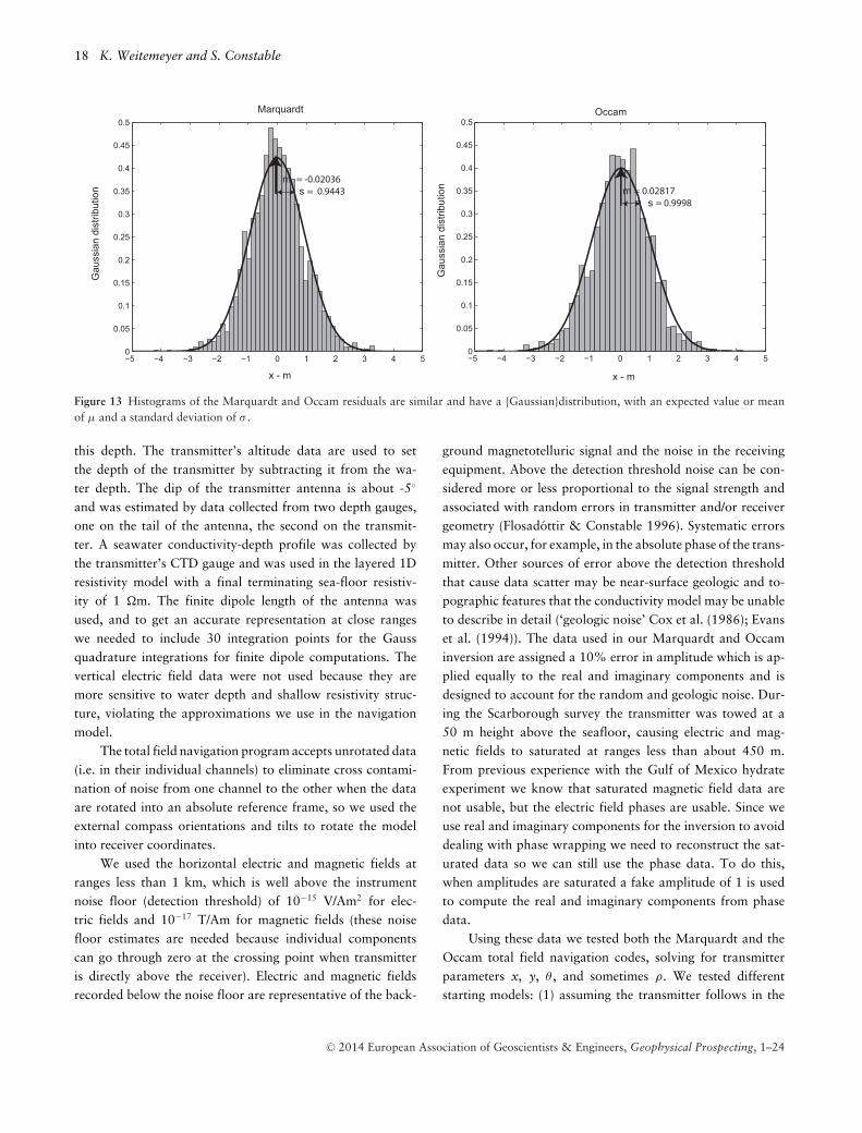
Figure 13 Histograms of the Marquardt and Occam residuals are similar and have a {Gaussian}distribution, with an expected value or meanof μ and a standard deviation of σ .
this depth. The transmitter’s altitude data are used to setthe depth of the transmitter by subtracting it from the wa-ter depth. The dip of the transmitter antenna is about -5◦
and was estimated by data collected from two depth gauges,one on the tail of the antenna, the second on the transmit-ter. A seawater conductivity-depth profile was collected bythe transmitter’s CTD gauge and was used in the layered 1Dresistivity model with a final terminating sea-floor resistiv-ity of 1 �m. The finite dipole length of the antenna wasused, and to get an accurate representation at close rangeswe needed to include 30 integration points for the Gaussquadrature integrations for finite dipole computations. Thevertical electric field data were not used because they aremore sensitive to water depth and shallow resistivity struc-ture, violating the approximations we use in the navigationmodel.
The total field navigation program accepts unrotated data(i.e. in their individual channels) to eliminate cross contami-nation of noise from one channel to the other when the dataare rotated into an absolute reference frame, so we used theexternal compass orientations and tilts to rotate the modelinto receiver coordinates.
We used the horizontal electric and magnetic fields atranges less than 1 km, which is well above the instrumentnoise floor (detection threshold) of 10−15 V/Am2 for elec-tric fields and 10−17 T/Am for magnetic fields (these noisefloor estimates are needed because individual componentscan go through zero at the crossing point when transmitteris directly above the receiver). Electric and magnetic fieldsrecorded below the noise floor are representative of the back-
ground magnetotelluric signal and the noise in the receivingequipment. Above the detection threshold noise can be con-sidered more or less proportional to the signal strength andassociated with random errors in transmitter and/or receivergeometry (Flosadottir & Constable 1996). Systematic errorsmay also occur, for example, in the absolute phase of the trans-mitter. Other sources of error above the detection thresholdthat cause data scatter may be near-surface geologic and to-pographic features that the conductivity model may be unableto describe in detail (‘geologic noise’ Cox et al. (1986); Evanset al. (1994)). The data used in our Marquardt and Occaminversion are assigned a 10% error in amplitude which is ap-plied equally to the real and imaginary components and isdesigned to account for the random and geologic noise. Dur-ing the Scarborough survey the transmitter was towed at a50 m height above the seafloor, causing electric and mag-netic fields to saturated at ranges less than about 450 m.From previous experience with the Gulf of Mexico hydrateexperiment we know that saturated magnetic field data arenot usable, but the electric field phases are usable. Since weuse real and imaginary components for the inversion to avoiddealing with phase wrapping we need to reconstruct the sat-urated data so we can still use the phase data. To do this,when amplitudes are saturated a fake amplitude of 1 is usedto compute the real and imaginary components from phasedata.
Using these data we tested both the Marquardt and theOccam total field navigation codes, solving for transmitterparameters x, y, θ , and sometimes ρ. We tested differentstarting models: (1) assuming the transmitter follows in the
C© 2014 European Association of Geoscientists & Engineers, Geophysical Prospecting, 1–24
Transmitter navigation in marine electromagnetic surveys 19
010203040506070265270275280285290295300305
Hea
ding
(de
gree
s)
0 10 20 30 40 50 60 70
−50
0
50
100
δY
(m
)iLBL solution - Marquardt model
0 20 30 40 50 60 70
−100
−50
0
50
100
δX
(m
)
0 10 20 30 40 50 60 70
−10−5
05
10152025
δθ(
degr
ees)
transmitter index
0 10 20 30 40 50 60 70
RM
S M
isfit
87654321
UT
M N
orth
ing
(km
)
UTM Easting (km)731 731.5 732 732.5 733 733.5 734
7796
7796.2
7796.4
7796.6
7796.8
7797
7797.2
site 19
site 20
site 21
site 22
site 23
site 24
iLBL
layback from ship
iLBL
layback from ship
iLBL-layback from ship
iLBL-layback from ship
iLBL-layback from ship
iLBL0.25 Hz0.75 Hz1.25 Hz1.75 Hz3.25 Hz4.25 Hzlayback from ship(starting model)
transmitter index
(a)
(b)
(c)
(d)
(e)
(f)
all frequencies
10
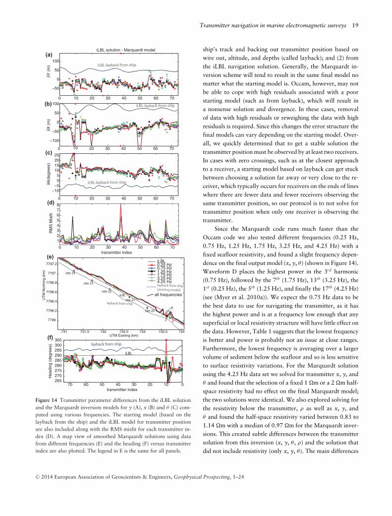
Figure 14 Transmitter parameter differences from the iLBL solutionand the Marquardt inversion models for y (A), x (B) and θ (C) com-puted using various frequencies. The starting model (based on thelayback from the ship) and the iLBL model for transmitter positionare also included along with the RMS misfit for each transmitter in-dex (D). A map view of smoothed Marquardt solutions using datafrom different frequencies (E) and the heading (F) versus transmitterindex are also plotted. The legend in E is the same for all panels.
ship’s track and backing out transmitter position based onwire out, altitude, and depths (called layback); and (2) fromthe iLBL navigation solution. Generally, the Marquardt in-version scheme will tend to result in the same final model nomatter what the starting model is. Occam, however, may notbe able to cope with high residuals associated with a poorstarting model (such as from layback), which will result ina nonsense solution and divergence. In these cases, removalof data with high residuals or reweighing the data with highresiduals is required. Since this changes the error structure thefinal models can vary depending on the starting model. Over-all, we quickly determined that to get a stable solution thetransmitter position must be observed by at least two receivers.In cases with zero crossings, such as at the closest approachto a receiver, a starting model based on layback can get stuckbetween choosing a solution far away or very close to the re-ceiver, which typically occurs for receivers on the ends of lineswhere there are fewer data and fewer receivers observing thesame transmitter position, so our protocol is to not solve fortransmitter position when only one receiver is observing thetransmitter.
Since the Marquardt code runs much faster than theOccam code we also tested different frequencies (0.25 Hz,0.75 Hz, 1.25 Hz, 1.75 Hz, 3.25 Hz, and 4.25 Hz) with afixed seafloor resistivity, and found a slight frequency depen-dence on the final output model (x, y, θ ) (shown in Figure 14).Waveform D places the highest power in the 3rd harmonic(0.75 Hz), followed by the 7th (1.75 Hz), 13th (3.25 Hz), the1st (0.25 Hz), the 5th (1.25 Hz), and finally the 17th (4.25 Hz)(see (Myer et al. 2010a)). We expect the 0.75 Hz data to bethe best data to use for navigating the transmitter, as it hasthe highest power and is at a frequency low enough that anysuperficial or local resistivity structure will have little effect onthe data. However, Table 1 suggests that the lowest frequencyis better and power is probably not an issue at close ranges.Furthermore, the lowest frequency is averaging over a largervolume of sediment below the seafloor and so is less sensitiveto surface resistivity variations. For the Marquardt solutionusing the 4.25 Hz data set we solved for transmitter x, y, andθ and found that the selection of a fixed 1 �m or a 2 �m half-space resistivity had no effect on the final Marquardt model;the two solutions were identical. We also explored solving forthe resistivity below the transmitter, ρ as well as x, y, andθ and found the half-space resistivity varied between 0.83 to1.14 �m with a median of 0.97 �m for the Marquardt inver-sions. This created subtle differences between the transmittersolution from this inversion (x, y, θ , ρ) and the solution thatdid not include resistivity (only x, y, θ ). The main differences
C© 2014 European Association of Geoscientists & Engineers, Geophysical Prospecting, 1–24

20 K. Weitemeyer and S. Constable
Table 1 Mean, median, and standard deviation of RMS misfit forvarious Marquardt models using data from different frequencies andall the frequencies simultaneously.
frequency mean RMS median RMS std dev.
0.25 Hz 1.22 0.98 1.050.75 Hz 1.29 1.17 0.641.25 Hz 1.55 1.37 0.851.75 Hz 1.51 1.38 0.673.25 Hz 1.77 1.76 0.644.25 Hz 2.11 2.09 0.680.75 Hz (ρ) 1.32 1.19 0.68all-frequencies (ρ) 1.85 1.65 0.81
occur at the closest approach to the receivers at the ends ofthe tow lines. We also inverted data from all 6 frequenciesand found that the models tended to fit to a slightly higherRMS of 1.85, probably dominated by the higher frequencies.The resulting model is similar to the previous models butwith less variation between neighbouring transmitter points.However, the model is still fairly rough, especially around site19.
In general all of the Marquardt solutions follow a similartrend, as shown in Figures 14. The region of closest approachto receiver number 19, where the transmitter crosses exactlyover the top of the receiver, has the most disagreement. Forall of the other receivers the transmitter is a few hundred me-ters or less to the north. Note that using the layback fromthe ship for the transmitter position places the transmitterincorrectly to the south of all the receivers, and gives a head-ing that is almost 15◦ different from the final solution. Thecenter of the antenna is also estimated by the iLBL model,rather than directly measured. This corrects the iLBL headingby about 10◦ and modifies the cross-line position by a me-dian of 33 m and the inline position by a median of about11 m.
We tested the Occam inversion using data with a fre-quency of 0.75 Hz and solved for transmitter x, y, θ , and ρ.The inversions were started from three different models, allhaving a half-space resistivity of 1 �m but differing startingtransmitter geometry: layback from the ship (model 1), thefinal smoothed Marquardt solution (model 2), and the iLBLnavigation geometry as shown in Figure 15 (model 3). Table2 shows the sequence of RMS as the models ran to conver-gence. We found that the Occam inversion scheme was sig-nificantly influenced by residuals greater than 50, becoming
−100
−50
0
50
100
δ x
(m)
0
10
20
δ θ(
degr
ees)
−0.2
0
0.2
0.4
δρ (Ω
m)
transmitter index
iLBL− ship layback
iLBL − smooth Marquardt
10 20 30 40 50 60 70
10 20 30 40 50 60 70
10 20 30 40 50 60 70
iLBL− ship layback
iLBL − smooth Marquardt
iLBL-inversion model
−100
−50
0
50
δ y(
m)
10 20 30 40 50 60 70
iLBL− ship laybackiLBL − smooth Marquardt
731 731.5 732 732.5 733 733.5 7347795.8
7796
7796.2
7796.4
7796.6
7796.8
7797
7797.2
7797.4
iLBL(start model 1)
site 19
ship layback(start model 1)
smooth Marquardt (start model 2)
Marquardt Occam starting from smoothed Marquardt (start model 2) fit to RMS 1.4Occam starting from ship layback (start model 1) fit to RMS 1.4Occam starting from iLBL (start model 3) fit to RMS 1.4Occam starting from iLBL (start model 3) fit to RMS 1.5
site 20
site 21
site 22
site 23
site 25
UTM Easting (km)
UT
M N
orth
ing
(km
)
270
280
290
Hea
ding
(de
g)
10203040506070
iLBLship layback
start smooth Marquardt
transmitter index
(a)
(b)
(c)
(d)
(e)
(f)
starting model: 1 Ωm
Figure 15 Comparing the various transmitter models from the iLBLsolution and the Occam total field navigation (TFN) solution, wherethree different starting models have been given to the Occam TFNinversion code (1) layback, (2), the Marquardt solution, (3) and theiLBL solution. The difference in y (A), x (B), θ (C) and ρ (D) areshown. A map view (E) of the final transmitter models for the surveyis also shown along with the heading versus transmitter index (F).The legend in E is the same for all panels.
C© 2014 European Association of Geoscientists & Engineers, Geophysical Prospecting, 1–24
Transmitter navigation in marine electromagnetic surveys 21
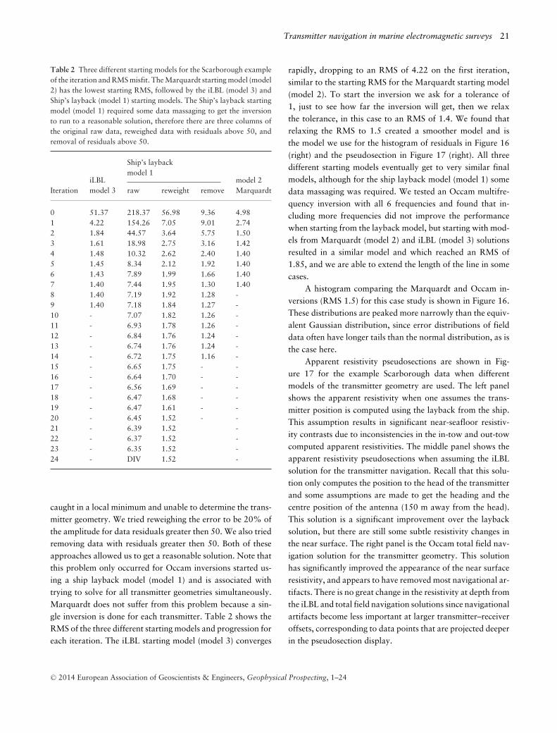
Table 2 Three different starting models for the Scarborough exampleof the iteration and RMS misfit. The Marquardt starting model (model2) has the lowest starting RMS, followed by the iLBL (model 3) andShip’s layback (model 1) starting models. The Ship’s layback startingmodel (model 1) required some data massaging to get the inversionto run to a reasonable solution, therefore there are three columns ofthe original raw data, reweighed data with residuals above 50, andremoval of residuals above 50.
Ship’s laybackmodel 1
iLBL model 2Iteration model 3 raw reweight remove Marquardt
0 51.37 218.37 56.98 9.36 4.981 4.22 154.26 7.05 9.01 2.742 1.84 44.57 3.64 5.75 1.503 1.61 18.98 2.75 3.16 1.424 1.48 10.32 2.62 2.40 1.405 1.45 8.34 2.12 1.92 1.406 1.43 7.89 1.99 1.66 1.407 1.40 7.44 1.95 1.30 1.408 1.40 7.19 1.92 1.28 -9 1.40 7.18 1.84 1.27 -10 - 7.07 1.82 1.26 -11 - 6.93 1.78 1.26 -12 - 6.84 1.76 1.24 -13 - 6.74 1.76 1.24 -14 - 6.72 1.75 1.16 -15 - 6.65 1.75 - -16 - 6.64 1.70 - -17 - 6.56 1.69 - -18 - 6.47 1.68 - -19 - 6.47 1.61 - -20 - 6.45 1.52 - -21 - 6.39 1.52 -22 - 6.37 1.52 -23 - 6.35 1.52 -24 - DIV 1.52 -
caught in a local minimum and unable to determine the trans-mitter geometry. We tried reweighing the error to be 20% ofthe amplitude for data residuals greater then 50. We also triedremoving data with residuals greater then 50. Both of theseapproaches allowed us to get a reasonable solution. Note thatthis problem only occurred for Occam inversions started us-ing a ship layback model (model 1) and is associated withtrying to solve for all transmitter geometries simultaneously.Marquardt does not suffer from this problem because a sin-gle inversion is done for each transmitter. Table 2 shows theRMS of the three different starting models and progression foreach iteration. The iLBL starting model (model 3) converges
rapidly, dropping to an RMS of 4.22 on the first iteration,similar to the starting RMS for the Marquardt starting model(model 2). To start the inversion we ask for a tolerance of1, just to see how far the inversion will get, then we relaxthe tolerance, in this case to an RMS of 1.4. We found thatrelaxing the RMS to 1.5 created a smoother model and isthe model we use for the histogram of residuals in Figure 16(right) and the pseudosection in Figure 17 (right). All threedifferent starting models eventually get to very similar finalmodels, although for the ship layback model (model 1) somedata massaging was required. We tested an Occam multifre-quency inversion with all 6 frequencies and found that in-cluding more frequencies did not improve the performancewhen starting from the layback model, but starting with mod-els from Marquardt (model 2) and iLBL (model 3) solutionsresulted in a similar model and which reached an RMS of1.85, and we are able to extend the length of the line in somecases.
A histogram comparing the Marquardt and Occam in-versions (RMS 1.5) for this case study is shown in Figure 16.These distributions are peaked more narrowly than the equiv-alent Gaussian distribution, since error distributions of fielddata often have longer tails than the normal distribution, as isthe case here.
Apparent resistivity pseudosections are shown in Fig-ure 17 for the example Scarborough data when differentmodels of the transmitter geometry are used. The left panelshows the apparent resistivity when one assumes the trans-mitter position is computed using the layback from the ship.This assumption results in significant near-seafloor resistiv-ity contrasts due to inconsistencies in the in-tow and out-towcomputed apparent resistivities. The middle panel shows theapparent resistivity pseudosections when assuming the iLBLsolution for the transmitter navigation. Recall that this solu-tion only computes the position to the head of the transmitterand some assumptions are made to get the heading and thecentre position of the antenna (150 m away from the head).This solution is a significant improvement over the laybacksolution, but there are still some subtle resistivity changes inthe near surface. The right panel is the Occam total field nav-igation solution for the transmitter geometry. This solutionhas significantly improved the appearance of the near surfaceresistivity, and appears to have removed most navigational ar-tifacts. There is no great change in the resistivity at depth fromthe iLBL and total field navigation solutions since navigationalartifacts become less important at larger transmitter–receiveroffsets, corresponding to data points that are projected deeperin the pseudosection display.
C© 2014 European Association of Geoscientists & Engineers, Geophysical Prospecting, 1–24

22 K. Weitemeyer and S. Constable
−15 −10 −5 0 5 10 150
0.1
0.2
0.3
0.4
0.5
0.6
x - m
Gau
ssia
n di
strib
utio
n
m =0.001007
s = 1.5496
Marquardt
−15 −10 −5 0 5 10 150
0.1
0.2
0.3
0.4
0.5
0.6
m =-0.013635
s = 1.5005
Occam
x - m
Figure 16 Histogram of Occam residuals for an RMS Misfit = 1.5 (right) and Marquardt residuals (left). In this case four parameters solvedfor: x, y, θ , ρ.
731.5 732 732.5 733 733.5
1000
1200
1400
1600
1800
2000
2200
2400
Easting (km)
pseu
do−
dept
h (
m)
s19s20s21s22s23s24
731.5 732 732.5 733 733.5
1000
1200
1400
1600
1800
2000
2200
2400
Easting (m)
pseu
do−
dept
h (
m)
s19s20s21s22s23s24
731.5 732 732.5 733 733.5
1000
1200
1400
1600
1800
2000
2200
2400
Easting (km)
pseu
do−
dept
h (m
)
appa
rent
res
istiv
ity (
Ω m
)
0.5
1
1.5
2
2.5
3
s19s20s21s22s23s24
731 731.5 732 732.5 733 733.5 7347795.8
7796
7796.2
7796.4
7796.6
7796.8
7797
7797.2
7797.4
site 19
ship layback
site 20
site 21
site 22
site 23
site 25
UTM Easting (km)
UT
M N
orth
ing
(km
)
270
280
290
Rot
atio
n (d
eg)
10203040506070transmitter index
731 731.5 732 732.5 733 733.5 7347795.8
7796
7796.2
7796.4
7796.6
7796.8
7797
7797.2
7797.4
site 19
site 20
site 21
site 22
site 23
site 25
UTM Easting (km)
UT
M N
orth
ing
(km
)
270
280
290
Rot
atio
n (d
eg)
10203040506070transmitter index
731 731.5 732 732.5 733 733.5 7347795.8
7796
7796.2
7796.4
7796.6
7796.8
7797
7797.2
7797.4
site 19
Occam starting from iLBL fit to RMS 1.5
site 20
site 21
site 22
site 23
site 25
UTM Easting (km)
UT
M N
orth
ing
(km
)
270
280
290
Rot
atio
n (d
eg)
10203040506070transmitter index
iLBL
0.75 Hz Layback(start model 1)
0.75 Hz iLBL(start model 3)
0.75 Hz TFN(final solution)
Figure 17 Apparent resistivity pseudosections of the Scarborough example when the navigation used is computed from the layback (left), theiLBL (middle), and the TFN (right) - the faint dots on top of the pseudosections are the data projections. The navigational parameters used tomake the pseudosections are shown in the middle (map view of survey layout) and bottom row (heading angle of the transmitter).
10 CONCLUSIONS
We have shown that the electromagnetic radiation pattern ofa dipole may be used to solve for CSEM transmitter naviga-tion parameters, since antenna heading, dip, height, inline andcrossline position all produce distinct patterns as a functionof range and frequency. A synthetic model demonstrates theviability of the algorithm and provided a basis for using a realdata set from the Scarborough gas field, Australia, for whicheither a Marquardt or Occam inversion of short range electric
and magnetic field data can be used to estimate transmittergeometry. The solution is well constrained because multiplereceivers observe a single transmitter. While this method isuseful to improve navigation in CSEM surveys it also demon-strates the sensitivity of each of the EM components to thegeometry of the transmitter, especially at ranges shorter than750 m. We found that the Occam inversion scheme may con-verge to a local minimum under the influence of a few largedata residuals. In these cases, re-weighting or removing the
C© 2014 European Association of Geoscientists & Engineers, Geophysical Prospecting, 1–24
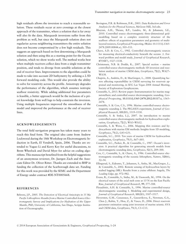
Transmitter navigation in marine electromagnetic surveys 23
high residuals allows the inversion to reach a reasonable so-lution. These residuals occur at zero crossings at the closestapproach of the transmitter, where a solution that is far awaywill also fit the data. Marquardt inversions suffer from thisproblem as well, but since the Marquardt solution does notregularize across neighboring transmitters the entire solutiondoes not become compromised by a few high residuals. Thissuggests an approach based on first determining a Marquardtsolution and then using this as a starting point for the Occamsolution, which we show works well. The method works bestwhen multiple receivers collect data from a single transmitterposition, and tends to diverge from sensible solutions at theend of receiver lines. Improvements to the algorithm could bemade to take into account 2D bathymetry by utilizing a 2.5Dforward modeling code. This would also provide the abilityto solve for resistivity across the profile. Anisotropy degradesthe performance of the algorithm, which assumes isotropicseafloor resistivity. While adding additional free parametersis feasible, a better approach would be the inclusion of a pri-ori knowledge from well logs to help constrain the inversion.Using multiple frequencies improved the smoothness of themodel and improved the performance at the end of receiverlines.
ACKNOWLEDGE ME N T S
The total field navigation program has taken many years toreach this final form. The original idea came from AndrewLockwood during the 18th Workshop on Electromagnetic In-duction in Earth, El Vendrell, Spain, 2006. Thanks are ex-tended to Yuguo Li and Kerry Key for useful discussions, toBrent Wheelock and David Myer for advice on coding algo-rithms. This manuscript benefited from the helpful suggestionsof an anonymous reviewer, Dr. Juergen Zach and the Asso-ciate Editor Dr. Oliver Ritter. Thanks are extended to BHP infunding the collection of the Scarborough data set. Fundingfor this work was provided by the SEMC and the Departmentof Energy under contract #DE-NT0005668.
REFERENCES
Behrens, J.P., 2005. The Detection of Electrical Anisotopy in 35 MaPacific Lithosphere: Results from a Marine Controlled-Source Elec-tromagnetic Survey and Implications for Hydration of the UpperMantle, PhD, University of California, San Diego, Scripps Institu-tion of Oceanography.
Bevington, P.R. & Robinson, D.K., 2003. Data Reduction and ErrorAnalysis for the Physical Sciences, McGraw Hill, 3rd edn.
Bhuyian, A.H., Thrane, B.P., Landro, M., & Johansen, S.E.,2010. Controlled source electromagnetic three-dimensional grid-modelling based on a complex resistivity structure of theseafloor: effects of acquisition parameters and geometry of multi-layered resistors, Geophysical Prospecting, 58(doi: 10.1111/j.1365-2478.2009.00844.x), 505–533.
Chave, A.D. & Cox, C., 1982. Controlled electromagnetic sourcesfor measuring electrical-conductivity beneath the oceans .1. For-ward problem and model study, Journal of Geophysical Research,87(NB7), 5327–5338.
Christensen, N.B. & Dodds, K., 2007. Special section – marinecontrolled-source electromagnetic methods 1D inversion and reso-lution analysis of marine CSEM data, Geophysics, 72(2), WA27–WA38.
Chuprin, A., Andreis, D., & MacGregor, L., 2008. Quantifying fac-tors affecting repeatablility in CSEM surveying for reservoir ap-praisal and monitoring, in SEG Las Vegas 2008 Annual Meeting,Society of Exploration Geophysicists.
Constable, S., 2013. Review paper: Instrumentation for marine mag-netotelluric and controlled source electromagnetic sounding, Geo-physical Prospecting, 10.1111/j.1365-2478.2012.01117.x, 1365–2478.
Constable, S. & Cox, C.S., 1996. Marine controlled-source electro-magnetic sounding 2. The PEGASUS experiment, Journal of Geo-physical Research, 101(B3), 5519–5530.
Constable, S. & Srnka, L.J., 2007. An introduction to marinecontrolled-source electromagnetic methods for hydrocarbon explo-ration, Geophysics, 72(2), WA3–WA12.
Constable, S. & Weiss, C., 2006. Mapping thin resistors and hy-drocarbons with marine EM methods: Insights from 1D modeling,Geophysics, 71(2), G43–G51.
Constable, S.C., 2010. Ten years of marine CSEM for hydrocarbonexploration, Geophysics, 75(5), A67–A81.
Constable, S.C., Parker, R., & Constable, C., 1987. Occam’s inver-sion: A practical algorithm for generating smooth models fromelectromagnetic sounding data, Geophysics, 52(3), 289–300.
Cox, C., Constable, S., & Chave, A., 1986. Controlled-source elec-tromagnetic sounding of the oceanic lithosphere, Nature, 320(6),52–54.
Ellingsrud, S., Eidesmo, T., Johansen, S., Sinha, M., MacGregor, L.,& Constable, S., 2002. Remote sensing of hydrocarbon layers byseabed logging (SBL): Results from a cruise offshore Angola, TheLeading Edge, pp. 972–982.
Evans, R., Constable, S., Sinha, M., & Unsworth, M., 1994. On theelectrical nature of the axial melt zone at 13◦N on the East PacificRise, Journal of Geophysical Research, 99, 577–588.
Flosadottir, A.H. & Constable, S., 1996. Marine controlled-sourceelectromagnetic sounding 1. Modeling and experimental design,Journal of Geophysical Research, 101(B3), 5507–5517.
Hoversten, G.M., Cassassuce, F., Gasoerikova, E., Newman, G.A.,Chen J., Rubin, Y., Hou, Z., & Vasco, D., 2006. Direct reservoirparameter estimation using joint inversion of marine seismic AVAand CSEM data, Geophysics, 71(3), C1–C13.
C© 2014 European Association of Geoscientists & Engineers, Geophysical Prospecting, 1–24

24 K. Weitemeyer and S. Constable
Key, K., 2009. 1D inversion of multicomponent, multifrequency ma-rine CSEM data: Methodology and synthetic studies for resolvingthin resistive layers, Geophysics, 74(2), 9–20.
Key, K. & Constable, S. C., 2011. An inverted long-baseline naviga-tion system for deep-towed em transmitter systems, in MARELEC,La Jolla CA. USA.
Key, K. & Lookwood, A., 2010. Determining the orientation of ma-rine CSEM receivers using orthogonal procrustes rotation analysis,Geophysics, 75(3), F63–F70.
Kong, F., 2007. Hankel transform filters for dipole antenna radia-tion in a conductive medium, Geophysical Prospecting, 55, 83–89.
Lien, M. & Mannseth, T., 2008. Sensitivity study of marine CSEMdata for reservoir production monitoring, Geophysics, 73(4), 151–163.
Marquardt, D.W., 1963. An algorithm for least-squares estimationof nonlinear parameters, Journal of the Society for Industrial andApplied Mathematics, 11(2), 431–441.
Martinez, Y., Allegar, N., Thomsen, L.A., & Stoyer, C., 2010.Method for determining electromagnetic survey sensor orientation,United States Patent Application Publication 20100102820A1.
Mittet, R., Aakervik, O.M., Jensen, H.R., Ellingsrud, S., & Stovas,A., 2007. On the orientation and absolute phase of marine CSEMreceivers, Geophysics, 72(4), F145–F155.
Myer, D., Constable, S., & Key, K., 2010a. Broad-band waveformsand robust processing for marine csem surveys, Geophysical Jour-nal International.
Myer, D., Constable, S., & Key, K., 2010b. A marine EM surveyof the Scarborough gas field, Northwest Shelf of Australia, FirstBreak, 28, 77–82.
Myer, D., Constable, S., Key, K., Glinsky, M.E., & Liu, G., 2012.
Marine CSEM of the Scarborough gas field, Part 1: Experimentaldesign and data uncertainty, Geophysics, 77(4), E281–E299.
Orange, A., Key, K., & Constable, S., 2009. The feasibility of reservoirmonitoring using time-lapse marine csem, Geophysics, 74(2), F21–F29.
Streich, R. & Becken, M., 2010. Electromagnetic fields generated byfinite-length wire sources: comparison with point dipole sources,Geophysical Prospecting, 59(2), 361–374.
Summerfield, P., Gale, L., Lue, X., Phillips, T., Quintanilla, R.,Eriksen, E., Rutledge, A., & Solon, K., 2005. Marine CSEM ac-quisition challenges, Society of Exploration Geophysicists Houston2005 Annual Meeting.
Swidinsky, A. & Edwards, R.N., 2011. Joint inversion of navigationand resistivity using a fixed transmitter and a towed receiver ar-ray: a transient marine CSEM model study, Geophysical JournalInternational, pp. 1–10.
Ward, S.H. & Hohmann, G.W., 1987. Electromagnetic Methods inApplied Geophysics, vol. 1 of Investigations in Geophysics, chap.4 Electromagnetic Theory for Geophysical Applications, pp. 131–311, Society of Exploration Geophysicists.
Weitemeyer, K., Constable, S., Key, K., & Behrens, J., 2006. Firstresults from a marine controlled-source electromagnetic survey todetect gas hydrates offshore Oregon, Geophysical Research Letters,33(L03304), doi:10.1029/2005GL024896.
Weitemeyer, K.A., 2008. Marine Electromagnetic Methods for GasHydrate Characterization, Ph.D. thesis, University of California,San Diego, La Jolla CA. USA.
Zach, J., Frenkel, M., Ridyard, D., Hincapie, J., Dubois, B., &Morten, J.P., 2009. Marine CSEM time-lapse repeatability for hy-drocarbon field monitoring, in SEG Technical Program ExpandedAbstracts.
C© 2014 European Association of Geoscientists & Engineers, Geophysical Prospecting, 1–24