navigation and tracking applications - link¶ping university
TRANSCRIPT
Linkoping Studies in Science and Technology. DissertationsNo. 579
Recursive Bayesian EstimationNavigation and Tracking Applications
Niclas Bergman
Department of Electrical EngineeringLinkoping University, SE–581 83 Linkoping, Sweden
Linkoping 1999

Cover Illustration: The front cover depicts a terrain elevation map covering a southern part ofthe province of Ostergotland, Sweden. Bright color indicates a high terrain elevation value. Thecorresponding terrain information, or variation, for the same area is shown on the back cover. Thevisible large dark areas are the lakes Sommen and Asunden. The Baltic sea and the archipelago ofVastervik are visible in the east part of the map. The terrain information on the cover is part of alarge map used in the terrain navigation application, presented in Chapter 2 and Chapter 7. Similarillustrations with further explanations are given on page 8 of the thesis.
Recursive Bayesian Estimation:Navigation and Tracking Applications
c© 1999 Niclas Bergman
http://www.control.isy.liu.se
Department of Electrical EngineeringLinkoping UniversitySE–581 83 Linkoping
Sweden
ISBN 91-7219-473-1 ISSN 0345-7524
Printed in Sweden by Linus & Linea AB


Abstract
Recursive estimation deals with the problem of extracting information about pa-rameters, or states, of a dynamical system in real time, given noisy measurementsof the system output. Recursive estimation plays a central role in many appli-cations of signal processing, system identification and automatic control. In thisthesis we study nonlinear and non-Gaussian recursive estimation problems in dis-crete time. Our interest in these problems stems from the airborne applications oftarget tracking, and autonomous aircraft navigation using terrain information.
In the Bayesian framework of recursive estimation, both the sought parame-ters and the observations are considered as stochastic processes. The conceptualsolution to the estimation problem is found as a recursive expression for the pos-terior probability density function of the parameters conditioned on the observedmeasurements. This optimal solution to nonlinear recursive estimation is usuallyimpossible to compute in practice, since it involves several integrals that lack ana-lytical solutions.
We phrase the application of terrain navigation in the Bayesian framework, anddevelop a numerical approximation to the optimal but intractable recursive solu-tion. The designed point-mass filter computes a discretized version of the posteriorfilter density in a uniform mesh over the interesting region of the parameter space.Both the uniform mesh resolution and the grid point locations are automaticallyadjusted at each iteration of the algorithm. This Bayesian point-mass solution isshown to yield high navigation performance in a simulated realistic environment.
Even though the optimal Bayesian solution is intractable to implement, theperformance of the optimal solution is assessable and can be used for compara-tive evaluation of suboptimal implementations. We derive explicit expressions forthe Cramer-Rao bound of general nonlinear filtering, smoothing and predictionproblems. We consider both the cases of random and nonrandom modeling of theparameters. The bounds are recursively expressed and are connected to linear re-cursive estimation. The newly developed Cramer-Rao bounds are applied to theterrain navigation problem, and the point-mass filter is verified to reach the boundin exhaustive simulations.
The uniform mesh of the point-mass filter limits it to estimation problems oflow dimension. Monte Carlo methods offer an alternative approach to recursiveestimation and promise tractable solutions to general high dimensional estimationproblems. We provide a review over the active field of statistical Monte Carlomethods. In particular, we study the particle filters for recursive estimation. Threedifferent particle filters are applied to terrain navigation, and evaluated against theCramer-Rao bound and the point-mass filter. The particle filters utilize an adaptivegrid representation of the filter density and are shown to yield a performance equalto the point-mass method.
A Markov Chain Monte Carlo (MCMC) method is developed for a highly com-plex data association problem in target tracking. This algorithm is compared topreviously proposed methods and is shown to yield competitive results in a simu-lation study.
i


Preface
Some of the results of this thesis have, or will, appear as published material. Thework was initially focused on the application of terrain navigation, which resultedin the conference papers
[15] N. Bergman. A Bayesian approach to terrain-aided navigation. In Proc. ofSYSID’97, 11th IFAC Symposium on System Identification, pages 1531–1536.IFAC, 1997,
[23] N. Bergman, L. Ljung, and F. Gustafsson. Point-mass filter and Cramer-Raobound for terrain-aided navigation. In Proc. 36:th IEEE Conf. on decisionand control, pages 565–570, 1997
and the Licentiate thesis
[16] N. Bergman. Bayesian Inference in Terrain Navigation. Linkoping Studies inScience and Technology. Thesis No 649, 1997.
Most results on terrain navigation presented in this thesis can be found in [16]. Theterrain navigation application nicely encompasses the major concepts of the generalproblem of nonlinear recursive estimation, and is therefore used as an extensiveintroduction to the thesis presented in Chapter 2. This chapter is an exact copy ofthe forthcoming article
[24] N. Bergman, L. Ljung, and F. Gustafsson. Terrain navigation using Bayesianstatistics. IEEE Control Systems Magazine, 19(3), June 1999.
The results on Cramer-Rao bounds presented in Chapter 4 and Section 7.2 arecovered by
[23] N. Bergman, L. Ljung, and F. Gustafsson. Point-mass filter and Cramer-Raobound for terrain-aided navigation. In Proc. 36:th IEEE Conf. on decisionand control, pages 565–570, 1997.
[25] N. Bergman and P. Tichavsky. Two Cramer-Rao bounds for terrain-aidednavigation. IEEE Transactions on Aerospace and Electronic Systems, 1999.In review.
The wavelet approach to spatial grid adaptation of Section 5.3 has been presentedas
[20] N. Bergman. An interpolating wavelet filter for terrain navigation. In Proc. conf.on multisource-multisensor information fusion, pages 251–258, 1998.
The Monte Carlo methods for terrain navigation given in Section 7.4 have, andwill, appear as
[18] N. Bergman. Deterministic and stochastic Bayesian methods in terrain navi-gation. In Proc. 37:th IEEE Conf. on Decision and Control, 1998.
iii

iv
[21] N. Bergman. Terrain navigation using sequential Monte Carlo methods. InA. Doucet, J.F.G. de Freitas, and N.J. Gordon, editors, Sequential Monte Carlomethods in practice. Cambridge University Press, 1999. To appear.
Part of the results on target tracking in Chapter 8 will be published in
[22] N. Bergman and F. Gustafsson. Three statistical batch algorithms for trackingmanoeuvring targets. In Proc. 5th European Control Conference, Karlsruhe,Germany, 1999.
Material not directly covered by the thesis, but nevertheless related to the conceptsin Chapter 8, is found in
[93] A. Isaksson, F. Gustafsson, and N. Bergman. Pruning versus merging inKalman filter banks for manoeuvre tracking. IEEE Transactions on Aerospaceand Electronic Systems, 1999. Accepted for publication.

Acknowledgments
My supervisors Professor Fredrik Gustafsson and Professor Lennart Ljung deservemy deepest gratitude. This thesis is to a large extent a results of their skillfulguidance and encouraging support of my work. I am extra grateful to Fredrik forall the fruitful, spontaneous discussions we have had during this work.
Several other distinguished researchers have supported me in this work. Iwould like to thank Arnaud Doucet for introducing me to the field of statisti-cal Monte Carlo methods, and taking care of me during my visit to Cambridge.Petr Tichavsky is acknowledged for introducing me to the posterior Cramer-Raobound, and Andrew Logothetis for sharing the tracking application with me.
Parts of the manuscript have at different stages been reviewed by ArnaudDoucet, Fredrik Tjarnstrom, Fredrik Gunnarsson, and Urban Forssell. Their valu-able comments and suggestions have lifted the thesis to a level I never would havereached on my own.
This work has been partly sponsored by ISIS, a NUTEK Competence Cen-ter at Linkoping University. The simulation data and the terrain database havebeen provided by Saab Dynamics, Linkoping Sweden. Detailed explanations aboutthe navigation application have also been provided by several employees of Saab,Linkoping.
Linkoping, April 1999
Niclas Bergman
v

vi

Contents
1 Introduction 1
1.1 Thesis Outline . . . . . . . . . . . . . . . . . . . . . . . . . . . . . . 11.2 Contributions . . . . . . . . . . . . . . . . . . . . . . . . . . . . . . . 31.3 Reading Directions . . . . . . . . . . . . . . . . . . . . . . . . . . . . 3
2 Terrain Navigation using Bayesian Statistics 5
2.1 Aircraft Navigation . . . . . . . . . . . . . . . . . . . . . . . . . . . . 62.2 The Bayesian Approach to Terrain Navigation . . . . . . . . . . . . . 92.3 The Point-Mass Filter . . . . . . . . . . . . . . . . . . . . . . . . . . 122.4 Simulation Evaluation . . . . . . . . . . . . . . . . . . . . . . . . . . 152.5 Conclusion . . . . . . . . . . . . . . . . . . . . . . . . . . . . . . . . 192.6 Acknowledgment . . . . . . . . . . . . . . . . . . . . . . . . . . . . . 19
3 Bayesian Estimation 21
3.1 Notational Conventions . . . . . . . . . . . . . . . . . . . . . . . . . 223.2 Bayesian Estimation . . . . . . . . . . . . . . . . . . . . . . . . . . . 23
3.2.1 Estimates . . . . . . . . . . . . . . . . . . . . . . . . . . . . . 243.3 Parametric Inference . . . . . . . . . . . . . . . . . . . . . . . . . . . 273.4 Sensor Fusion . . . . . . . . . . . . . . . . . . . . . . . . . . . . . . . 29
3.4.1 Estimation Error Covariance . . . . . . . . . . . . . . . . . . 30
vii

viii Contents
3.4.2 Optimal Fusion of Estimates . . . . . . . . . . . . . . . . . . 303.4.3 Dempster-Shafer Combination . . . . . . . . . . . . . . . . . 32
3.5 Recursive Estimation . . . . . . . . . . . . . . . . . . . . . . . . . . . 343.5.1 Conceptual Solution . . . . . . . . . . . . . . . . . . . . . . . 363.5.2 Linear Recursive Estimation . . . . . . . . . . . . . . . . . . 393.5.3 Nonlinear Recursive Estimation . . . . . . . . . . . . . . . . . 403.5.4 Continuous Time Filtering . . . . . . . . . . . . . . . . . . . . 43
3.6 Summary . . . . . . . . . . . . . . . . . . . . . . . . . . . . . . . . . 44
3.A Foundational Concepts of Probability Theory . . . . . . . . . . . . . 453.A.1 Probability Theory . . . . . . . . . . . . . . . . . . . . . . . . 453.A.2 Random Variables . . . . . . . . . . . . . . . . . . . . . . . . 46
4 Cramer-Rao Bounds 49
4.1 Review over Cramer-Rao Bounds . . . . . . . . . . . . . . . . . . . . 504.1.1 Estimator Performance . . . . . . . . . . . . . . . . . . . . . 514.1.2 Nonrandom Parameters . . . . . . . . . . . . . . . . . . . . . 524.1.3 Random Parameters . . . . . . . . . . . . . . . . . . . . . . . 55
4.2 Discrete Time Nonlinear Estimation . . . . . . . . . . . . . . . . . . 564.2.1 Background . . . . . . . . . . . . . . . . . . . . . . . . . . . . 564.2.2 Estimation Model . . . . . . . . . . . . . . . . . . . . . . . . 57
4.3 Parametric Bounds . . . . . . . . . . . . . . . . . . . . . . . . . . . . 594.3.1 Fictitious Measurements . . . . . . . . . . . . . . . . . . . . . 594.3.2 Bound Calculations . . . . . . . . . . . . . . . . . . . . . . . 61
4.4 Posterior Bounds . . . . . . . . . . . . . . . . . . . . . . . . . . . . . 644.5 Relative Monte Carlo Evaluation . . . . . . . . . . . . . . . . . . . . 684.6 Conclusions . . . . . . . . . . . . . . . . . . . . . . . . . . . . . . . . 70
4.A Vector Gradients and Matrix Inversions . . . . . . . . . . . . . . . . 724.A.1 Vector Gradients . . . . . . . . . . . . . . . . . . . . . . . . . 724.A.2 Two Common Matrix Inversion Relations . . . . . . . . . . . 73
4.B Proof of General Cramer-Rao Bounds . . . . . . . . . . . . . . . . . 734.B.1 Proof of Theorem 4.1 . . . . . . . . . . . . . . . . . . . . . . 754.B.2 Proof of Theorem 4.2 . . . . . . . . . . . . . . . . . . . . . . 76
4.C Proof of Bounds for Recursive Estimation . . . . . . . . . . . . . . . 774.C.1 Proof of Theorem 4.3 . . . . . . . . . . . . . . . . . . . . . . 774.C.2 Proof of Theorem 4.5 . . . . . . . . . . . . . . . . . . . . . . 794.C.3 Proof of Theorem 4.6 . . . . . . . . . . . . . . . . . . . . . . 794.C.4 Proof of Theorem 4.7 . . . . . . . . . . . . . . . . . . . . . . 80
5 Grid Based Methods 83
5.1 The Curse of Dimensionality . . . . . . . . . . . . . . . . . . . . . . 855.2 The Point-Mass Filter . . . . . . . . . . . . . . . . . . . . . . . . . . 87
5.2.1 Background . . . . . . . . . . . . . . . . . . . . . . . . . . . . 875.2.2 Point-Mass Approximation . . . . . . . . . . . . . . . . . . . 895.2.3 Grid Adaption . . . . . . . . . . . . . . . . . . . . . . . . . . 91
Contents ix
5.2.4 Implementation . . . . . . . . . . . . . . . . . . . . . . . . . . 935.3 Spatially Adaptive Grid . . . . . . . . . . . . . . . . . . . . . . . . . 965.4 Conclusion . . . . . . . . . . . . . . . . . . . . . . . . . . . . . . . . 99
6 Simulation Based Methods 101
6.1 Monte Carlo Integration and Optimization . . . . . . . . . . . . . . . 1026.1.1 Integration . . . . . . . . . . . . . . . . . . . . . . . . . . . . 1036.1.2 Optimization . . . . . . . . . . . . . . . . . . . . . . . . . . . 105
6.2 Classical Methods of Sampling . . . . . . . . . . . . . . . . . . . . . 1066.2.1 Rejection Sampling . . . . . . . . . . . . . . . . . . . . . . . . 1076.2.2 Importance Sampling . . . . . . . . . . . . . . . . . . . . . . 1086.2.3 Summary . . . . . . . . . . . . . . . . . . . . . . . . . . . . . 110
6.3 Markov Chain Monte Carlo . . . . . . . . . . . . . . . . . . . . . . . 1106.3.1 Theory . . . . . . . . . . . . . . . . . . . . . . . . . . . . . . 1116.3.2 Algorithms . . . . . . . . . . . . . . . . . . . . . . . . . . . . 113
6.4 Recursive Monte Carlo Methods . . . . . . . . . . . . . . . . . . . . 1186.4.1 Algorithms . . . . . . . . . . . . . . . . . . . . . . . . . . . . 1196.4.2 Implementational Issues . . . . . . . . . . . . . . . . . . . . . 1276.4.3 Applications . . . . . . . . . . . . . . . . . . . . . . . . . . . 130
6.5 Summary . . . . . . . . . . . . . . . . . . . . . . . . . . . . . . . . . 130
7 Terrain Navigation 133
7.1 Application Background . . . . . . . . . . . . . . . . . . . . . . . . . 1347.1.1 Integration of Navigation Systems . . . . . . . . . . . . . . . 1357.1.2 Approaches to Terrain Navigation . . . . . . . . . . . . . . . 137
7.2 Cramer-Rao Bound Evaluation . . . . . . . . . . . . . . . . . . . . . 1417.3 Terrain Information . . . . . . . . . . . . . . . . . . . . . . . . . . . 1467.4 Monte Carlo Filters . . . . . . . . . . . . . . . . . . . . . . . . . . . 1477.5 Conclusion . . . . . . . . . . . . . . . . . . . . . . . . . . . . . . . . 156
8 Target Tracking 157
8.1 The Expectation Maximization Algorithm . . . . . . . . . . . . . . . 1588.1.1 A Target Tracking Example . . . . . . . . . . . . . . . . . . . 160
8.2 Multiple Measurement Data Association . . . . . . . . . . . . . . . . 1638.2.1 Problem Formulation . . . . . . . . . . . . . . . . . . . . . . 1648.2.2 Multiple Simultaneous Measurement Filter . . . . . . . . . . 1668.2.3 Expectation Maximization Data Association . . . . . . . . . 1678.2.4 Markov Chain Monte Carlo Data Association . . . . . . . . . 1698.2.5 Simulation Result . . . . . . . . . . . . . . . . . . . . . . . . 174
8.3 Conclusion . . . . . . . . . . . . . . . . . . . . . . . . . . . . . . . . 178
8.A Expectation Maximization for Segmentation . . . . . . . . . . . . . . 180
9 Conclusive Remarks 185
Bibliography 187

x Contents
Notation 199
Index 203

1
Introduction
Nonlinear and non-Gaussian recursive estimation problems are commonly encoun-tered, e.g., in target tracking and navigation applications. Practical solutions tothese problems usually resort to model approximations, applying standard linearsolutions to local linearizations of the estimation model. This will yield algorithmswith modest computational requirements, but will clearly be suboptimal when thenonlinearities of the problem are severe. The local linearization schemes thereforefail in applications where detailed nonlinear models are available and the estimationperformance cannot be sacrificed.
In this work, we emphasize the Bayesian view on statistical inference and reviewthe tools available for approximative implementation of this approach to nonlinearrecursive estimation. Instead of describing the problem model approximatively, theoptimal solution is here implemented in an approximative fashion.
1.1 Thesis Outline
The next chapter is an exact copy of the submitted final manuscript to [24]. Thisarticle highlights the major problems of recursive estimation by studying the terrainnavigation application in detail. It is this application that has been the foundationalapplication, propelling the work presented in this thesis. The chapter contains abrief presentation of the terrain navigation application, its Bayesian solution, and
1

2 Introduction
an approximative numerical integration method developed with this application inmind. This introduction serves both to exemplify the type of problems we consider,and to present the main results obtained for the terrain navigation application.There will inevitably be some overlap between Chapter 2 and the rest of the thesis,in particular when we return to the terrain navigation application in Chapter 7.
Chapter 3 contains a comprehensive review over estimation theory with anemphasis on the Bayesian paradigm of statistical inference. The review aims at de-scribing the Bayesian view of statistical inference in general, and its application tothe recursive estimation problem in particular. The chapter also contains commentson optimal combination of sensor measurements and clarifies some connections be-tween classical statistical inference and the inference method of Dempster–Shafer.A review over approaches to nonlinear recursive estimation is also given in Chap-ter 3.
In Chapter 4 we present bounds on the mean square estimation error in recursiveestimation. Firstly, we review and extend the basic results of Cramer-Rao boundsfor both random and parametric estimation. Secondly, these bounds are applied tothe recursive estimation problem. We derive recursive expressions for the Cramer-Rao bounds to filtering prediction and smoothing in nonlinear, non-Gaussian statespace models. The presentation is streamlined by emphasizing the obtained resultsand postponing all proofs to appendices to the chapter.
In Chapter 5, we consider a direct approach to implementing the optimalBayesian solution by means of numerical integration. This leads to grid basedmethods that recursively computes a discretized version of the posterior filter den-sity. We exemplify such methods by presenting a grid based method specificallydeveloped for the terrain navigation application. We also comment the difficultiesin applying grid based methods to problems of high dimension, and presents someresults on adapting the grid spatially.
Chapter 6 contains a review over simulation based methods, which are bettersuited for high dimensional problems. In these Monte Carlo methods, statisticalinference is performed by simulating a large number of candidate parameters andcomputing sample averages with respect to these. We review the general conceptof Monte Carlo methods and present the basic theoretical justifications for theirproperties along with several algorithms. Most importantly, we present the MonteCarlo methods for recursive estimation.
In Chapter 7, we return to the terrain navigation application and describethe integration between terrain navigation and inertial navigation. Different ap-proaches to terrain navigation are reviewed and compared to the Bayesian approachsuggested in this work. We combine the grid based method for Bayesian terrainnavigation of Chapter 5 with the Cramer-Rao bounds of Chapter 4. In extensivesimulations we show that the implementation reach a nearly optimal performancelevel with a densely chosen grid resolution. Comparative simulation studies betweenthe grid based method, Cramer-Rao bound, and some algorithms from Chapter 6are also provided.
Chapter 8 contains applications of Bayesian inference to problems in targettracking. Firstly, we review the Expectation Maximization (EM) algorithm and

1.2 Contributions 3
apply it to a target manoeuvre detection problem. Secondly, we study a complexdata association problem occuring in over the horizon target tracking. We develop aGibbs sampling procedure for this problem and compare it to two other previouslysuggested approaches. The applications of target tracking that we consider areoff-line algorithms and therefore fall slightly out of scope, judging form the title ofthe thesis. Chapter 8 instead serves to illustrate Bayesian techniques in general,and some concepts of Chapter 6 in particular.
Finally, Chapter 9 provides some conclusive remarks regarding the work, andpossible directions of future research.
1.2 Contributions
Chapter 3 and Chapter 6 contain overviews of statistical Bayesian estimation andnumerical Monte Carlo methods, respectively. The complementary chapters con-tain the main contributions of the thesis, they are listed below in order of appear-ance.
• The Bayesian formulation of, and solution to, the terrain navigation problem,presented in Chapter 2.
• The parametric Cramer-Rao bounds for filtering, prediction, and smoothingin nonlinear, and non-Gaussian, recursive state space estimation problems.The bounds are presented in Chapter 4.
• The posterior Cramer-Rao bounds for singular state evolution and for smooth-ing in nonlinear and non-Gaussian recursive estimation, also given in Chap-ter 4.
• The numerical integration point-mass filter developed for the terrain naviga-tion, detailed in Chapter 5.
• The Cramer-Rao bounds and particle filters for terrain navigation, presentedin Chapter 7.
• The Gibbs sampling procedure for multiple measurement data association,described in Chapter 8.
1.3 Reading Directions
Readers primarily interested in the terrain navigation application may read Chap-ter 2, and thereafter resort to Section 5.2 and Chapter 7. Complementary informa-tion about the intricate details of the terrain navigation application can be foundin the Licentiate thesis [16]. However, the Bayesian approach to this problem, andits solution, is fully covered in this work.
Readers with an aim to solely study the parts on the Cramer-Rao bounds forrecursive estimation are suggested to go directly to Chapter 4. The basic concepts

4 Introduction
of estimation theory can be found in Chapter 3 if a prior knowledge of statisticalestimation is lacking. Illustrations of the practical application of the bounds arefound in Section 7.2, Section 7.3, and Section 7.4.
The review of Monte Carlo methods in Chapter 6 is to a large extent self-contained and may be read without reference to the other chapters. However,it will prove beneficial to consult Section 7.4 and Section 8.2 to exemplify andilluminate the concepts presented in Chapter 6.

2
Terrain Navigation using
Bayesian Statistics
In aircraft navigation the demands on reliability and safety are very high. Theimportance of accurate position and velocity information becomes crucial whenflying an aircraft at low altitudes, and especially during the landing phase. Notonly should the navigation system have a consistent description of the position ofthe aircraft, but also a description of the surrounding terrain, buildings and otherobjects that are close to the aircraft. Terrain navigation is a navigation scheme thatutilizes variations in the terrain height along the aircraft flight path. Integratedwith an Inertial Navigation System (INS), it yields high performance position es-timates in an autonomous manner, i.e., without any support information sent tothe aircraft. In order to obtain these position estimates, a nonlinear recursiveestimation problem must be solved on-line. Traditionally, this filtering problemhas been solved by local linearization of the terrain at one or several assumed air-craft positions. Due to changing terrain characteristics, these linearizations willin some cases result in diverging position estimates. In this work, we show howthe Bayesian approach gives a comprehensive framework for solving the recursiveestimation problem in terrain navigation. Instead of approximating the model ofthe estimation problem, the analytical solution is approximately implemented. Theproposed navigation filter computes a probability mass distribution of the aircraftposition and updates this description recursively with each new measurement. Thenavigation filter is evaluated over a commercial terrain database, yielding accu-rate position estimates over several types of terrain characteristics. Moreover, in a
5

6 Terrain Navigation using Bayesian Statistics
Monte Carlo analysis, it shows optimal performance as it reaches the Cramer-Raolower bound.
2.1 Aircraft Navigation
Navigation is the concept of determination of the kinematic state of a movingvehicle. In aircraft navigation this usually consists of finding the position andvelocity of the aircraft. Accurate knowledge of this state is critical for flight safety.Therefore, an aircraft navigation system should not only provide a reliable andaccurate estimate of the current kinematic state of the aircraft, but also a consistentdescription of the accuracy of this estimate.
Aircraft navigation is typically performed using a combination of dead-reckoningand fix position updates. In dead-reckoning systems, the state vector is calculatedfrom a continuous series of measurements of the aircraft movement relative to aninitial position. Due to error accumulation, dead-reckoning systems must be re-initialized periodically. Fix point, or positioning, systems measure the state vectormore or less without regard to the previous movement of the aircraft. They aretherefore suitable for re-initialization of dead-reckoning systems.
The most common dead-reckoning systems are the Inertial Navigation Systems(INS) in which accelerometers are used to sense the magnitude of the aircraft accel-eration. A set of gyroscopes either maintains the accelerometers in a known orien-tation with respect to a fixed, non-rotating coordinate system, commonly referredto as inertial space, or measures the angular rate of the accelerometers relativeto inertial space. The inertial navigation computer uses these sensed accelerationsand angular rates to compute the aircraft velocity, position, attitude, attitude rate,heading, altitude, and possibly range and bearing to destination. An INS generatesnear instantaneous continuous position and velocity, it is self-contained, functionsat all latitudes, and in all weather conditions. It operates independently of air-craft manoeuvres and without the need for ground station support. Complete andcomprehensive presentations of inertial navigation can be found in [99, 135].
Positioning systems that have attracted a lot of attention lately are the globalsatellite navigation systems which promise a very high accuracy and global cov-erage. There are two global satellite systems for navigation in use today: GPS,developed by the U.S., and the Russian system GLONASS. Position estimates areobtained by comparing distances from the aircraft to four or more satellites. Thesystems have been developed for military purposes and several coding techniquesare used to keep the accuracy for civilian or unauthorized users at a level far fromthe actual performance of the systems. However, using ground stations as reference,the coding errors can be removed efficiently. Vendors have off-the-shelf receiversfor differential GPS (DGPS) with a position accuracy below the one meter level. Acomprehensive summary of the concept of satellite navigation can be found in [99,Chapter 5].
The radio navigation systems have the disadvantage of relying on informationbroadcasted to the aircraft. This information could be deliberately jammed in

2.1 Aircraft Navigation 7
a hostile situation, or the transmitters could be destroyed, leaving the aircraftwithout navigation support. Hence, even if the satellite systems give high accuracyposition information they need to be combined with alternative backup systems us-ing other navigation principles. The concept of terrain navigation is an alternativepositioning technique that autonomously generates updates to the INS, althoughin general not with the same accuracy as the satellite systems. The main idea interrain navigation is to measure the variations in the terrain height underneath theaircraft flight path and compare these measurements with a reference map. The
Altitude Ground clearance
Mean sea-level
Terrain elevation
Figure 2.1: The principle of terrain navigation.
principle of terrain navigation is depicted in Figure 2.1. The aircraft altitude overmean sea-level is measured with a barometric altimeter and the ground clearanceis measured with a radar altimeter, pointing downward. The terrain elevation be-neath the aircraft is found by taking the difference between the altitude and groundclearance measurements. The navigation computer holds a digital reference mapwith values of the terrain elevation as a function of longitude and latitude. Themeasured terrain elevation is compared with this reference map and matching po-sitions in the map are determined. Terrain repetitiveness and flatness make thismatching nontrivial and the quality of the outcome dependent on the amount ofterrain variation. Many areas inside the reference map will in general have a ter-rain elevation comparable to the measured one. In order to distinguish the trueposition from false ones, several measurements along the aircraft flight path needto be considered. Hence, the measurements must be matched with the map on-lineand in a recursive manner. For comprehensive discussions about the applicationsof terrain navigation techniques, see [86, 87].

8 Terrain Navigation using Bayesian Statistics
The performance of the matching of terrain elevation measurements with themap depends highly on the type of terrain in the area. Flat terrain gives little orno information about the aircraft position. Rough, but repetitive, terrain can giveseveral well matched positions in an area, making it hard to distinguish betweenseveral, well matching tracks. The information content inside a generic area of themap can be shown to be proportional to the average size of the terrain gradient,√√√√ 1
N
N∑i=1
‖∇h(xi)‖2 (2.1)
where xi are positions uniformly distributed in the area of interest. This scalarmeasure of the terrain information can be connected to an associated Cramer-Raobound for the underlying estimation problem [16]. The right part of Figure 2.2shows (2.1) evaluated in square blocks of 400 meter side where bright color indicatesa large value. The terrain map used in this work is a real commercial map of a 100
Figure 2.2: The left part shows the terrain height and the right part the informationcontent in the map over a central part of Sweden.
by 100 km area of central Sweden. The pure terrain elevation samples are given ina uniform mesh of 50 by 50 meter resolution and shown to the left in the figure.Using interpolation from surrounding map values, the terrain map can be regardedas a known look-up table of terrain elevations as a function of position. Everythingthat in the real world cannot be found by interpolation from the database valuesmust be regarded as noise. The right part of Figure 2.2 very clearly shows the lakes,and the coastline of the Baltic sea to the right in the map. The north-west partof the map is flat agricultural land with very little navigation information, whilethe southern part consists of very rough terrain with varying hills of some hundredmeters height and narrow valleys that give a high information content. Maps such

2.2 The Bayesian Approach to Terrain Navigation 9
as the right part of Figure 2.2 could be used for mission planning purposes, e.g.,finding the most informative path to the final destination.
There are several commercial algorithms that solve the terrain navigation prob-lem. Since the development has been driven by military interests, most of theseare not very well documented in the literature. The most frequently referred algo-rithms for terrain navigation are TERCOM (terrain contour matching) and SITAN(Sandia inertial terrain-aided navigation). TERCOM is batch oriented and corre-lates gathered terrain elevation profiles with the map periodically [6, 75, 135]. Theaircraft is not allowed to maneuver during data acquisition in TERCOM and there-fore it has mainly been used for autonomous crafts, like cruise missiles. SITAN isrecursive and uses a modified version of an extended Kalman filter (EKF) in itsoriginal formulation [91]. When flying over fairly flat or over very rough terrain,or when the aircraft is highly maneuverable, this algorithm does not in generalperform well. In order to overcome these divergence problems parallel EKFs havebeen used in [31, 88]. Another widespread system is the TERPROM system, devel-oped by British Aerospace, can be found in several NATO aircraft. It is a hybridsolution, in which an acquisition-mode correlates measurements in batch to findan initial position and in track-mode processes measurements recursively usingKalman filter techniques. However, due to commercial interests and because of itsuse as a classified military system, it is not as well documented in the literature asthe previous two. One more recent and different approach that tries to deal withthe nonlinear problems is VATAN [64]. In VATAN the Viterbi algorithm is ap-plied to the terrain navigation problem, yielding a maximum a posteriori positionestimate.
In this work, we take a completely statistical view on the problem and solve thematching with the map as a recursive nonlinear estimation problem. The concep-tual solution is described in the following section and an approximate implemen-tation in Section 2.3. Simulation results with this implementation are presentedSection 2.4.
2.2 The Bayesian Approach to Terrain Navigation
As shown in Figure 2.1 the difference between the altitude estimate and the mea-sured ground clearance yields a measurement of the terrain elevation. Assumingadditive measurement noise the terrain elevation yt relates to the current aircraftposition xt according to
yt = h(xt) + et (2.2)
where the function h(·) : R2 7→ R is the terrain elevation map. The measurementnoise et is a white process with some known distribution pet(·). This measurementerror models both the errors in the radar altimeter measurements, the current al-titude estimate and errors originating from the interpolation in the terrain mapnot perfectly resembling the real world. Let ut denote the estimate of the rela-tive movement of the aircraft between two measurements obtained from the INS.

10 Terrain Navigation using Bayesian Statistics
Modeling the dead-reckoning drift of the INS with a white additive process vt, theabsolute movement of the aircraft obeys a simple linear relation
xt+1 = xt + ut + vt (2.3)
where vt is distributed according to some assumed known probability density func-tion pvt(·). Summarizing equations (2.2) and (2.3) yields the nonlinear model
xt+1 = xt + ut + vt
yt = h(xt) + ett = 0, 1 . . . (2.4)
where vt and et are mutually independent white processes, both of them uncorre-lated with the initial state x0 which is distributed according to p(x0). One mayargue that the INS estimate ut should be regarded as a sensor measurement insteadof as a known parameter in the state transition equation,
ut = xt+1 − xt + eINSt .
This would require the introduction of a new state vector incorporating both xt andxt+1 in order to retain the Markovian property of the state space model. Instead,we choose to include the error eINS
t in the process noise vt in (2.4). This limitsthe state dimension and drastically reduces the computational power required torecursively compute an approximation of the conditional density of the states.
The objective of the terrain navigation algorithm is to estimate the currentaircraft position xt using the observations collected until present time
Yt = yiti=0.
With a Bayesian approach to recursive filtering, everything worth knowing aboutthe state at time t is condensed in the conditional density p(xt |Yt). With someabuse of notation, the distribution of a generic random variable z conditioned onanother related random variable w is
p(z |w) =p(z , w)p(w)
=p(w | z) p(z)
p(w)(2.5)
Assume that p(xt |Yt−1) is known and apply (2.5) to the last member in the setYt,
p(xt |Yt) =p(yt |xt , Yt−1) p(xt |Yt−1)
p(yt |Yt−1).
Inserting the model (2.4) and noting that the denominator is a scalar normalizationconstant yield,
p(xt |Yt) = α−1t pet(yt − h(xt)) p(xt |Yt−1)
αt =∫pet(yt − h(xt))p(xt |Yt−1) dxt

2.2 The Bayesian Approach to Terrain Navigation 11
which describes the influence of the measurement. Using (2.5) the joint density ofthe states at two measurement instants is
p(xt+1 , xt) = p(xt+1 |xt) p(xt).
The density update between two measurements is found by marginalizing this ex-pression on the state xt and inserting (2.4),
p(xt+1 |Yt) =∫pvt(xt+1 − xt − ut)p(xt |Yt) dxt.
This completes one iteration of the recursive solution. Summarizing the deriva-tion, the Bayesian formula for updating the conditional density is initiated byp(x0 |Y−1) = p(x0) and calculated as
p(xt |Yt) = α−1t pet(yt − h(xt)) p(xt |Yt−1)
p(xt+1 |Yt) =∫pvt(xt+1 − xt − ut)p(xt |Yt) dxt
(2.6)
where
αt =∫pet(yt − h(xt))p(xt |Yt−1) dxt.
The Bayesian solution is a density function describing the distribution of the statesgiven the collected measurements. From the conditional density, a point estimatesuch as the minimum mean square error estimate can be formed
xt =∫xt p(xt |Yt) dxt. (2.7)
Assuming that this estimate is unbiased, the covariance
Ct =∫
(xt − xt)(xt − xt)T p(xt |Yt) dxt (2.8)
quantizes the accuracy of the estimate. Equation (2.8) is convenient when compar-ing (2.7) with estimates from other navigation systems.
The recursive update of the conditional density (2.6) describes how the mea-surement yt and the relative movement ut affect the knowledge about the aircraftposition. With each new terrain elevation measurement, the prior distributionp(xt |Yt−1) is multiplicatively amplified by the likelihood of the measurement yt.This means that the conditional probability will decrease in unlikely areas andincrease in areas where it is likely that the measurement was obtained. Betweentwo measurements, the density function p(xt |Yt) is translated according to therelative movement of the aircraft obtained from the INS and convolved with thedensity function of the error of this estimate. Thus the support and shape of theconditional density will adapt to areas which fit the measurements well and follow

12 Terrain Navigation using Bayesian Statistics
the movement obtained from the INS. It is worth noting that (2.6) is the Bayesiansolution to (2.4) for all possible nonlinear functions h(·) and for any noise distri-butions pvt(·) and pet(·). In the special case of linear measurement equation andGaussian distributed noises the equations above coincide with the Kalman filter [2].
Computationally, each iteration of the Bayesian solution (2.6) consists of solvingseveral integrals. Due to the unstructured nonlinearity h(·), these integrationsare in general impossible to solve in closed form and therefore there exists nosolution that updates the conditional density analytically. The implementationmust therefore inevitably be approximate. A straightforward way to implementthe solution is to simply evaluate the recursion in several positions inside the areawhere the aircraft is assumed to be and update these values further through therecursion. With such a quantization of the state space, the integrals in (2.6) turninto sums over the chosen point values. The earliest reference of such a numericalapproach to solving the nonlinear filtering problem is [34]. More recent referencesinvolve the p-vector approach in [137] and a slightly different approach, presentedin [103], using a piecewise constant approximation to the density function. In theterrain navigation problem the state dimension is two and the quantization can ingeneral be viewed as a bed-of-nails where the length of each nail corresponds toa certain elementary mass in that position. The implementation described in thispaper is therefore labeled the point-mass filter (PMF).
2.3 The Point-Mass Filter
Assume that N grid points in R2 have been chosen for the approximation ofp(xt |Yt). Introduce the notation
xt(k) k = 1, 2, . . . , N
for these N vectors in R2. Each of these N grid points has a corresponding prob-ability mass
p(xt(k) |Yt) k = 1, 2, . . . , N.
In order to obtain a simple and efficient algorithm, the grid points are chosen froma uniform rectangular mesh with resolution of δ meters between each grid point.Each integral operation in (2.6) is approximated by a finite sum over the grid pointswith nonzero weight
∫R2f(xt) dxt ≈
N∑k=1
f(xt(k)) δ2.

2.3 The Point-Mass Filter 13
Applying this approximation to (2.6) yields the Bayesian point-mass recursion:
p(xt(k) |Yt) = α−1t pet(yt − h(xt(k))) p(xt(k) |Yt−1)
xt+1(k) = xt(k) + ut k = 1, 2, . . . , N
p(xt+1(k) |Yt) =N∑n=1
pvt(xt+1(k)− xt(n)) p(xt(n) |Yt) δ2
(2.9)
where
αt =N∑k=1
pet(yt − h(xt(k))) p(xt(k) |Yt−1) δ2. (2.10)
The time update has been split into two parts. First the grid points are translatedwith the INS relative movement estimate ut and then the probability mass densityis convolved with the density pvt(·). The point estimate (2.7) is computed at eachiteration as the center of mass of the point-mass density,
xt =N∑k=1
xt(k)p(xt(k) |Yt) δ2.
Hence, the estimate does not necessarily fall on a grid point.In order to follow the aircraft movements the grid must be adapted to the
support of the conditional density. After each measurement update, every gridpoint with a weight less than ε > 0 times the average mass value
1N
N∑k=1
p(xt(k) |Yt) =1
Nδ2.
is removed from the grid. The new set of grid points is defined byxt(k) : p(xt(k) |Yt) > ε/Nδ2
.
The weights need to be re-normalized after this truncation operation. The trunca-tion will make the algorithm focus on areas with high probability and remove gridpoints in areas where the conditional density is small. The basic grid resolution δwill however not be affected by the truncation. When the algorithm is initialized,the uncertainty about the aircraft position is usually rather high. The prior willthen have a large support, and naturally it is not interesting to have a high gridresolution. Instead we start with a sparse grid and run the algorithm and removeweights using the truncation operation above until the number of remaining gridpoints falls below some threshold N0. Then the mesh resolution can be increasedand the algorithm continued to process new measurements, updating the condi-tional density in the new dense grid. The up-sampling is performed by placing onegrid point between every neighboring grid point in the mesh using linear interpo-lation to determine its weight. This will yield a doubling of the mesh resolution.

14 Terrain Navigation using Bayesian Statistics
The convolution in (2.9) will introduce some extra grid points along the border ofthe point-mass approximation, increasing the support of the mesh. If the measure-ments have low information content there will be a net-increase of grid points eventhough some are removed by the truncation operation. Therefore, if the number ofgrid points increases above some threshold N1, the mesh is decimated by removingevery second grid point from the mesh, halving the mesh resolution.
Hence, the number of grid points N , the point-mass support and the meshresolution δ is automatically adjusted through each iteration of the algorithm usingthe design parameters ε, N0 and N1. An illustration is given in Figure 2.6. Insummary the PMF algorithm consists of (2.9) and the appropriate resampling ofthe grid described above. Details about the implementation and the grid refinementprocedure can be found in [16].
The refinement of the grid support and resolution in the PMF described aboveis of course ad hoc, and one may wonder if this actually works. The Cramer-Raolower bound is a fundamental limit on the achievable algorithm performance whichcan be used to evaluate the average performance of the PMF and verify that thefilter solves the nonlinear filtering problem with near optimal performance. Theresults are presented here without proofs or derivations, see [16, 17, 23] for details.Let N(x;m,P ) denote the n-dimensional Gaussian distribution with mean vectorµ and covariance matrix P
N(x;µ, P ) = 1√(2π)n|P |
exp(− 1
2 (x− µ)TP−1(x− µ)).
Inserting Gaussian distributions in (2.4),
pet(et) = N(et; 0, Rt) pvt(vt) = N(vt; 0, Qt) p(x0) = N(x0; x0, P0),
the Cramer-Rao lower bound for the one step ahead prediction of the states satisfiesthe matrix (Riccati) recursion,
Pt+1 = Pt − PtHt(HTt PtHt +Rt)−1HT
t Pt +Qt
initiated with P0. Above Ht is the gradient of h(·) evaluated at the true state valueat time t,
Ht = ∇h(xt).
Thus, the Cramer-Rao bound is a function of the noise levels and the gradient ofthe terrain along the true state sequence.
The Cramer-Rao bound sets a lower limit on the estimation error covariancewhich depends on the statistical properties of the model (2.4) and on the algorithmused. A Monte Carlo simulation study is performed to determine the averageperformance of the algorithm for comparison with the Cramer-Rao bound. TheRoot Mean Square (RMS) Monte Carlo error for each fixed time instant is lowerbounded by the Cramer-Rao bound,√√√√ 1
M
M∑i=1
‖xt − xit‖2 &
√trPt
2.4 Simulation Evaluation 15
where xit is the one step ahead prediction of the states at time t in Monte Carlorun i.
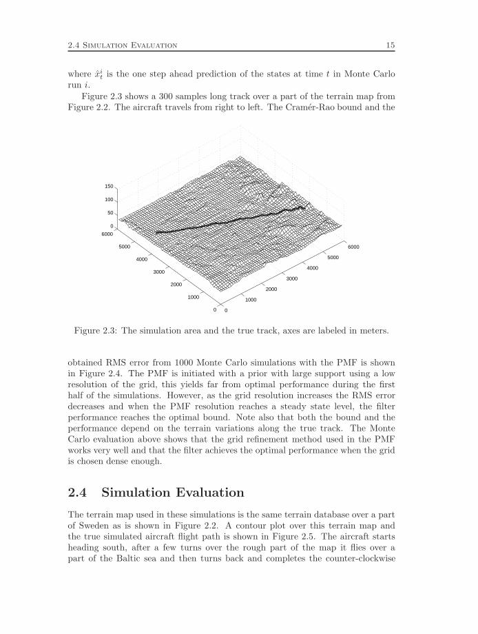
Figure 2.3 shows a 300 samples long track over a part of the terrain map fromFigure 2.2. The aircraft travels from right to left. The Cramer-Rao bound and the
0
1000
2000
3000
4000
5000
6000
0
1000
2000
3000
4000
5000
6000
0
50
100
150
Figure 2.3: The simulation area and the true track, axes are labeled in meters.
obtained RMS error from 1000 Monte Carlo simulations with the PMF is shownin Figure 2.4. The PMF is initiated with a prior with large support using a lowresolution of the grid, this yields far from optimal performance during the firsthalf of the simulations. However, as the grid resolution increases the RMS errordecreases and when the PMF resolution reaches a steady state level, the filterperformance reaches the optimal bound. Note also that both the bound and theperformance depend on the terrain variations along the true track. The MonteCarlo evaluation above shows that the grid refinement method used in the PMFworks very well and that the filter achieves the optimal performance when the gridis chosen dense enough.
2.4 Simulation Evaluation
The terrain map used in these simulations is the same terrain database over a partof Sweden as is shown in Figure 2.2. A contour plot over this terrain map andthe true simulated aircraft flight path is shown in Figure 2.5. The aircraft startsheading south, after a few turns over the rough part of the map it flies over apart of the Baltic sea and then turns back and completes the counter-clockwise

16 Terrain Navigation using Bayesian Statistics
0 50 100 150 200 250 3000
50
100
150
200
250
300
met
er
sample number
The Cramer-Rao lower boundMonte Carlo RMS error
Figure 2.4: Monte Carlo root mean square error compared with the Cramer-Raobound.
10 20 30 40 50 60 70 80 90 100
10
20
30
40
50
60
70
80
90
100
start
km
km
Figure 2.5: The simulation track over the terrain database.

2.4 Simulation Evaluation 17
lap. The simulated aircraft track, the INS measurements and the radar altimetermeasurements have all been generated in an advanced realistic simulator used bythe navigation systems development department at Saab Dynamics. The trackhas a duration of 25 minutes and is sampled at a rate of 10 Hz. The aircraft hasan average speed of Mach 0.55, and the manoeuvres are simulated as coordinatedturns.
The INS position estimate x0 is initiated with an error of 1000 m in both thenorth and the east direction. The prior density is chosen as a Gaussian distributioncentered at the erroneous INS estimate
p(x0) = N(x0; x0, 10002I2). (2.11)
The initial grid resolution used in the PMF to sample this function is δ = 200 m.The dead-reckoning drift in the INS is simulated as a constant bias of 1 m/s ineach channel. The distribution used in the algorithm to model this drift is Gaussianpvt(vt) = N(vt; 0, 4I2). The choice of Gaussian distributions has proven successfulin the simulations but any other suitable distribution that better models the po-sition drift and the initial uncertainty may be used. There is no restriction in thePMF to Gaussian noises: the only assumption is that the noise can be regarded aswhite.
Different sensor models are used when generating the simulated measurements.Depending on the terrain category beneath the aircraft at the measuring instant,both the bias and the variance of the radar altimeter are adjusted. For example,flying over dense forest the radar altimeter has a bias of 19 m with a large variance.Additional noise is added to the measurement to simulate that the radar altimetermeasurement performance degrades with increasing ground clearance distance. Thedensity used to capture these effects in the PMF algorithm is a mixture of twoGaussian distributions,
pet(et) = 0.8 N(et; 0, 2) + 0.2 N(et; 15, 9).
This choice can be interpreted as on the average every fifth measurement beingbiased due to reflection in trees or buildings. The truncation and resampling pa-rameters used in the PMF are,
ε = 10−3, N0 = 1000, N1 = 5000.
The simulation result from the first three recursions is depicted in Figure 2.6.Starting with the Gaussian prior (2.11), the first measurement amplifies the prob-ability in several regions and removes samples of low probability. After the secondrecursion, the grid resolution is increased to 100 m and the third recursion removeseven more samples and a single peak of the density shows the most probable aircraftposition while the uncertainty still is rather large. The bounding box indicatingthe support of the prior is shown as a comparison with the support of each of thefilter densities. The irregular shapes of these densities shows how the unstructurednonlinear terrain gives a filter density which is hard to approximate with smooth

18 Terrain Navigation using Bayesian Statistics
Prior Recursion 1
Recursion 2 Recursion 3
Figure 2.6: The first three recursions of the algorithm
0 5000 10000 1500010
−1
100
101
102
103
met
er
sample number
Figure 2.7: Estimation error along the simulation track, in logarithmic scale.

2.5 Conclusion 19
functions or local linearizations. Figure 2.7 shows the estimation error along thesimulation track. Here it is obvious that the performance depends on the coveredterrain. The error converges rapidly from the initial error of more than 1 km downto an error less than 30 m. When the aircraft reaches the Baltic sea the measure-ments have little information and the error increases with the drift of the INS.Once back over land, the estimate accuracy increases and a trend towards worseperformance is visible when the aircraft covers the low informative areas of themap during the final part of the lap. The resolution of the grid is automaticallyadjusted and varies between 200 m and 0.78 m along the simulation track. A com-mon navigation performance parameter is the circular error probable (CEP) whichis the median of the position error. The simulation yields a median error of 12.2 mCEP. As a comparison, in [88] an error of 50 m CEP is reported and in [31] a valueof 75 m is obtained. It should be remarked that both these values are found duringfield tests and not simulations.
2.5 Conclusion
The performance of terrain navigation depends on the size of the terrain gradientin the area. The point-mass filter described in this work yields an approximateBayesian solution that is well suited for the unstructured nonlinear estimationproblem in terrain navigation. It recursively propagates a density function of theaircraft position. The shape of the point-mass density reflects the estimate quality,this information is crucial in navigation applications where estimates from differ-ent sources often are fused in a central filter. The Monte Carlo simulations showthat the approximation can reach the optimal performance and the realistic simu-lations in Section 2.4 show that the navigation performance is very high comparedwith other algorithms and that the point-mass filter solves the recursive estimationproblem for all the types of terrain covered in the test.
The main advantages of the PMF is that it works for many kinds of nonlin-earities and many kinds of noise and prior distributions. The mesh support andresolution are automatically adjusted and controlled using a few intuitive designparameters. The main disadvantage is that it cannot solve estimation problems ofvery high dimension since the computational complexity of the algorithm increasesdrastically with the dimension of the state space. The implementation used in thiswork shows real-time performance for two dimensional and in some cases threedimensional models, but higher state dimensions are usually intractable.
2.6 Acknowledgment
The work has been partly sponsored by ISIS, a NUTEK Competence Center atLinkoping University. The simulation data and the terrain database have beenprovided by Saab Dynamics, Linkoping Sweden. Valuable detailed explanationsabout the navigation application have been provided by several employees of Saab,Linkoping.

20 Terrain Navigation using Bayesian Statistics

3
Bayesian Estimation
Statistical estimation deals with the problem of inferring knowledge about param-eters indirectly observable from the outcome of a related experiment. Usually, theexperiment is a measurement or observation of a real world phenomenon, and theparameter is a physical quantity that affects the measurement in a known manner.In recursive estimation, the inferred knowledge about the parameters is updatedcontinuously as new measurements are collected. This recursive processing of ob-servations is suitable in problems where the parameters have dynamic propertiesthat make them change with time, or when the application demands estimateswith certain frequency based on the sequence of measurements observed so far. Welabel the estimation problem recursive when there is a demand for such recursiveprocessing of the observations. With the Bayesian view on estimation, both thesought parameters and the observations are stochastic entities. This fundamentalparadigm yields a unifying framework for estimation problems where the inferenceresult is a conditional density function for the parameters given the observationaloutcome.
This chapter is a review of basic estimation theory and it serves as a theoreticalplatform for the sequel of the thesis. There are several excellent textbooks thatgive a much deeper and more thorough presentation of estimation theory thanfound herein. The book of Papoulis [120] presents the theory of probability andrandom processes from first principles. This reference also contains some interestinghistorical notes on the development of probability theory. A brief review of the
21

22 Bayesian Estimation
foundational concepts from probability theory is provided in the appendix to thischapter. The text in the appendix is based on [120]. Real valued parameters andobservations are considered throughout this chapter. A thorough measure theoreticpresentation of probability theory is given in the monograph by Chung [40].
The review of estimation theory presented in this chapter is mainly based on theclassical book of Van Trees [151]. Both the parametric and Bayesian approachesto estimation are given by Van Trees, and the connections between estimation anddetection are strongly emphasized. A complement to the rigorous book by VanTrees [151] that covers similar subjects in less detail is given by Scharf [130]. Arather theoretical, and purely Bayesian decision theoretic presentation of statisticalinference is given in the monograph of Robert [127]. This reference contains a strongargumentation in favor of the Bayesian paradigm in general. On the other side,the pure parametric viewpoint is given by Lehmann [109], who focuses on classicalinference where point estimators and their theoretical properties are presented ingreat depth.
Jazwinski [94] treats the recursive estimation problem both in continuous anddiscrete time, and for linear and nonlinear models. A more detailed presentation oflinear recursive estimation is given by Anderson and Moore [2], where only discretetime is considered. The manuscript of Kailath et al. [96] will probably be the keyreference to linear estimation when it finally goes into print.
3.1 Notational Conventions
A review of probability theory from the axiomatic definition to the concept ofconditional probability density functions is given in Appendix 3.A. This sectiongives a very brief summary of the notational conventions, described in more detailin Appendix 3.A.
Unless stated differently, x denotes a generic n-dimensional random parametervector and y a p-dimensional observation vector. Commonly in the literature, theword parameter is saved for nonrandom fixed entities while random entities are la-beled states. In the following section, we make no linguistical distinction betweenrandom and nonrandom entities, all sought entities are labeled parameters regard-less of if they are equipped with a prior distribution or not. Random variables aresometimes typed in bold face, x, when it serves to clarify the underlying meaning.Generally, p(x) denotes the probability density function for the random variablegiven in the argument, in this case x. When this rule does not apply, the randomvariable is indicated by a subscript, i.e., p(y)
y=x= py(x). Likewise, mathematical
expectation is performed w.r.t. all random variables given in the argument unlessa subscript indicates which variable should be affected by the integration, e.g.,E(f(x)) = Ex(f(x)).
The exact meaning of the conditional densities p(x | y) and p(y |x) is definedin Appendix 3.A. Expectation w.r.t. a conditional density is denoted E(x | y),and it follows the same subindex rule as regular expectation, e.g., E(f(x, y)) =Ey(E(f(x, y) | y)) = Ey(Ex|y(f(x, y))).

3.2 Bayesian Estimation 23
3.2 Bayesian Estimation
The objective of the estimation procedure is to gather information about the valueof the parameter x given an observation of an experimental outcome, y. In statisti-cal estimation it is customary to treat the observation y as a random vector, oftenjustified by assumptions about random measurement noise, imprecise measurementequipment or other unmodeled effects that may lend themselves for random mod-eling. The observation vector is assumed to have a probability density functionbelonging to a class indexed by the parameters, p(y |x). Hence, if the true parame-ter value was known, the complete statistical properties of the measurement wouldalso be known. In a Bayesian framework the parameter vector itself is also referredto as a random vector. The random vector x is assumed having a known priordensity function p(x). This prior distribution encompasses everything known, andunknown, about the parameters prior to observing the experimental outcome.
The result of the experiment is a realization of the random variable y. Observingthe event y = y yields, by means of Bayes’ law (3.A.24), that the knowledgeabout the parameters is altered so that
p(x | y) =p(y |x)p(x)
p(y). (3.1)
The meaning of this relation is described in detail in Appendix 3.A. With a purelyBayesian view on the estimation problem the posterior density function p(x | y)describes everything about the parameter x after the experimental outcome hasbeen observed. With the experiment result y at hand, the denominator of (3.1) isjust a scalar positive constant which can be found by marginalization,
p(y) =∫Rnp(y |x)p(x) dx.
Hence, in order to compute (3.1) one only needs to specify the product p(y |x)p(x).
Proposition 3.1A Bayesian estimation problem is defined by the joint density of the parameters andthe observations, p(x, y) = p(y |x)p(x).
From a Bayesian viewpoint, the likelihood and the prior, or alternatively the jointdensity, define the statistical model for the estimation problem, while the poste-rior (3.1) is its solution. Once the information y = y is at hand, the parameters,priorly regarded as the random variable x, should now be regarded as the randomvariable x | y. The posterior density can be used to deduce the probability of anycharacteristic of the parameter given the data. Hence, the posterior density shouldalways be regarded as the most general solution to the estimation problem even ifthe primary goal of the inference often is aimed at certain features of the posterior.

24 Bayesian Estimation
3.2.1 Estimates
The posterior is a general, but rather complex answer to the inference problem.Each candidate parameter value in Rn yields a value of p(x | y) reflecting the pos-terior probability of that parameter value. An estimate x is an educated guessof the parameter value given the observations at hand. It is often more desirableto determine an estimate than the complete posterior density. Each realization ofthe measurement yields a new estimate, and generally the rule of passing from anobservation to a parameter estimate is a function termed an estimator . Hence,an estimator is a function from the observation space to the parameter spacex : Rp → Rn. The argument of this function is explicitly indicated, x(y), onlywhen the dependency needs to be clarified. Note that the estimator should be re-garded as a random variable, since it is a function of the random variable y, whilethe estimate is a deterministic vector since it depends on the observed realizationy.
A natural way to find suitable estimators is to define a penalty for choosing anerroneous estimate. Let L(x(y), x) denote a cost function, reflecting a user definedpenalty for erroneous estimates x 6= x. In general, L(x, x) is defined such that thegreater the discrepancy x − x, the larger the cost. Without loss of generality, wecan assume that the cost function is positive and that L(x, x) = 0 is its uniqueminimum. The Bayesian risk R associated with an estimator x is defined as theexpected cost,
RM= E(L(x(y), x)) ,
where expectation is over both x and y. The optimal choice of x(y), using a costdefined by L(x(y), x), is the one that minimizes the Bayesian risk,
x(y) = arg minx?(y)
∫Rn+p
L(x?(y), x)p(x, y) dx dy,
where the minimization is over all possible functions x?(y). Inserting p(x, y) =p(x | y)p(y) splits the integration into two parts
x(y) = arg minx?(y)
∫Rp
∫RnL(x?(y), x)p(x | y) dx p(y) dy.
Since both L(x?, x) and p(x | y) are positive, the inner integral is positive given anyy. Furthermore, since p(y) also is positive, the value of x?(y) that minimizes therisk is the value that minimizes the inner integral,
x(y) = arg minx?(y)
∫RnL(x?(y), x)p(x | y) dx (3.2)
for each y. The optimization problem (3.2) defines the Bayesian estimation prob-lem and each choice of cost function gives different estimators. As an alternative

3.2 Bayesian Estimation 25
to (3.2), a minimax approach can be used. Then, the estimate that minimizes themaximal cost is chosen,
x(y) = arg minx?(y)
maxx
L(x?(y), x). (3.3)
In estimation problems it is often the case that the cost function only dependson the estimation error
xM= x− x,
and the abbreviated notation L(x − x) is used. This is no general considerationthough, there may, e.g., be situations where the cost of erroneously choosing certainestimates should be extra high since those estimates are used to take some crucialactions. This is exemplified at the end of this section. Nevertheless, the costfunction L(x) is rather general and can, e.g., handle cases when it is a much moresevere error to overestimate a quantity than to underestimate it. To illustrate theuse of cost functions to determine estimates, two standard choices of cost functionand their solutions to (3.2) follow below, see [151] for details.
First, we introduce a compact notation for quadratic norms. Let ‖x‖2AM= xTAx
for any square matrix A and compatible matrix or vector x, and introduce theabbreviated notation ‖x‖2 = ‖x‖2I . Moreover, let A > 0 denote that A is symmetricand positive definite. The, possibly weighted, mean-square error cost is defined by
LMS(x− x?) M= ‖x− x?‖2Q (3.4)
where Q > 0 is a weighting matrix. The minimum mean-square error estimate isthus defined by
xMSM= arg min
x?
∫Rn‖x− x?‖2Q p(x | y) dx.
Taking the gradient of the RHS integral w.r.t. x? and setting the result equal tozero yield
−2∫RnQxp(x | y) dx+ 2
∫RnQx? p(x | y) dx = 0 (3.5)
which is an equation for the unique minimum since the second derivative equals2Q > 0. Solving for x? yields that the optimal estimate in the mean-square senseis
xMS =∫Rnxp(x | y) dx. (3.6)
For obvious reasons, this estimate is also referred to as the conditional mean esti-mate.

26 Bayesian Estimation
Another common choice of cost function is the one that penalizes all errorsequally,
LUNIF(x− x?) M=
1 if ‖x− x?‖2 ≤ ∆2
0 if ‖x− x?‖2 > ∆2
given some small ∆ > 0. Then, as ∆→ 0, the optimal estimate is the maximum aposteriori estimate,
xMAPM= arg max
xp(x | y), (3.7)
which will coincide with the maximum likelihood estimate when an uninformativeprior p(x) is used. For a derivation of (3.7) see Van Trees [151].
The cost functions given above are the two most common choices for Bayesianpoint estimation. Some other examples of cost functions are given in [94, 151].One reason for the frequent use of these cost functions is the explicit form of theestimates (3.6) and (3.7), while for a generally chosen cost function, the estimate isonly implicitly defined through (3.2). Another reason for choosing the conditionalmean estimate is that it actually solves the general optimization problem (3.2) fora rather large class of cost functions, illustrated in the following two lemmas.
Lemma 3.1 (Property 1 of [151, p. 60])Let the cost function L(x) be a symmetric convex function, and assume that theposterior density is symmetric about its mean. Then, the optimal Bayesian esti-mator (3.2) is the conditional mean (3.6).
Lemma 3.2 (Property 2 of [151, p. 61])Let the cost function L(x) be symmetric and nondecreasing, and assume that theposterior density is symmetric about its mean, unimodal, and that it satisfies
limx→∞
L(x)p(x | y) = 0.
Then, the optimal Bayesian estimator (3.2) is the conditional mean (3.6).
Various interpretations of these two lemmas, together with proofs, can be foundin [2, 94, 151]. Throughout this thesis we will only consider conditional mean andmaximum a posteriori estimates.
The general framework of defining estimates through cost functions also ap-plies to hypothesis testing and decision problems, as illuminated by the followingexample.
Example 3.1 (Bayesian Detection Problem)Consider the problem of detecting a nonzero parameter vector x given a relatedobservation y. This problem is a binary hypothesis test with
H0 : x = 0H1 : x 6= 0

3.3 Parametric Inference 27
The estimate x is the output of the detector, thus it either accepts or rejects thehypothesis H0. The possible costs are defined by a (2 × 2) matrix
L(x, x) x = 0 x 6= 0x : choose H0 C00 C01
x : choose H1 C10 C11
(3.8)
With the prior density
p(x) =
P0 if x = 0.
P1 if x 6= 0.
inserted into (3.2) this will eventually lead to the well known likelihood ratiotest [130, 151]
p(y |x 6= 0)p(y |x = 0)
H1
≷H0
P0(C10 − C00)P1(C01 − C11)
.
Hence, x is chosen to H1 if the LHS is greater than the RHS, otherwise H0 ischosen.
The likelihood ratio test is obtained when choosing the decision that minimizes theBayesian risk (3.2), while the criterion (3.3) will lead to minimax type decisions.Detailed presentations of these concepts with deeper analogies between estimationand detection problems are carried out by Van Trees [151] and by Scharf [130].In (3.8) one usually distinguishes the cost for false alarm, C10, from that of misseddetection, C01. Thus, this is an example of a cost function which has differentcosts depending on both x and x, while for the estimates derived previously thecost function was a function only of the estimation error L(x).
3.3 Parametric Inference
With a so-called Fisherian, or parametric, view on estimation, the parameters arenot regarded as random variables. Instead, the sought parameters are regarded asfixed-but-unknown, and the parameter value explicitly affects the statistical proper-ties of the observation in a known manner. This connection between measurementand parameter is defined by a density function for the observation vector y param-eterized by the parameter vector x, denoted p(y |x). With a parametric view onestimation, p(y |x) is regarded as a function of the parameters after inserting themeasurement. Often, this likelihood function is written
l(x | y) M= p(y |x)
to emphasize that it is regarded as a function of the first argument after insertingthe observed y. Given the observed measurement y inserted into this function,the parameter vector x corresponding to the density most likely generating the

28 Bayesian Estimation
observed measurement is chosen. An estimate is thus formed by maximizing thelikelihood function,
xML = arg maxx
l(x | y)
this will lead to the theory of maximum likelihood estimation, rigorously presentedin [109]. With a very flat, also called uninformative, prior p(x), it is readily seenfrom (3.1) that the posterior will be almost proportional to the likelihood so thatthe Bayesian and parametric viewpoints in some sense coincide. Detailed pre-sentations over similarities and discrepancies between Bayesian and parametricstatistical estimation can be found in [33, 127].
It is sometimes argued that the demand for prior knowledge in order to definep(x) makes the Bayesian viewpoint less attractive. This should therefore favor theparametric approach where no such knowledge is needed. Moreover, the spokesmenfor the parametric view often claim that even if such prior knowledge exists it is hardto describe, at least in the form of a probability density function. Similar reasoningsays that since the choice of prior often is rather subjective, it may seriously alterthe resulting inference in a destructive way. These arguments speak in favor ofthe parametric viewpoint over the framework of Bayesian statistics. However,since both the likelihood and the prior define the inference problem according toProposition 3.1, picking the correct likelihood reflects the same problem as pickinga good prior.
In a practical situation we cannot guarantee that the real world observationsthat we base our inference on are exactly drawn from the probability model definedby the joint density p(x, y). Likewise, there is no way to assure that the measure-ments we collect origin from a parameterized density function p(y |x) given somex in the set of admissible parameters. Both these frameworks are merely modelswhere statistics is used to describe a complex reality. If the reality was exactly de-scribed by, e.g., the model p(x, y), the complete solution is given by the posteriordensity p(x | y). If this is not the case, but we still base our inference and computeour estimates with respect to the density p(x, y), it is an issue of robustness againstmodeling errors. Detailed discussions in this topic along with means to introducerobustness into Bayesian inference is given by Berger [14], Box and Tiao [33].
The need for defining a prior knowledge is not a demand but an option. Choos-ing an uninformative prior attenuates its effect on the inference result, while aprior with a well defined support will be clearly visible in the estimate. Hence, theBayesian approach can be seen as a generalization of the parametric approach withan option to bias the result by choosing the support and shape of the prior density.Robert [127] delivers a strong argumentation in favor of the Bayesian viewpointover the parametric one. General guidelines to the choice of prior distribution aregiven by Berger [14], Box and Tiao [33] and Robert [127].

3.4 Sensor Fusion 29
3.4 Sensor Fusion
Conceptually, inference based on several sensors can be performed within either ofthe frameworks for statistical inference reviewed above. Since we allow for a vectorvalued observation, the measurement vector can straightforwardly be assembledfrom two physical measurements provided by different sensors. The statistical de-pendency between the two sensors is controlled by the choice of likelihood. Com-bining, e.g., two sensor outputs, y1 and y2, with independent measurement noise,a likelihood on the form
p(y |x) = p(y1, y2 |x) = p(y1 |x)p(y2 |x) (3.9)
is a suitable choice. However, inference at this high level of generality is oftennot practically possible. Either the features that the sensors measure or the typeof information they produce are usually so different that it is hard to model thebehavior of all sensors in a complete framework of the type (3.9). Moreover, im-plementational constraints often induce that most processing of data need to beexecuted locally, at each sensor. This may put constraints on the inference thatare hard to incorporate in the framework of (3.9).
The general problem of combining information regarding an object, or severalobjects, and the surrounding environment is commonly referred to as the sensorfusion problem. The key difference between traditional statistical inference andsensor fusion is that the information considered is of fundamentally different formand provided on different levels of abstraction. Surveys over the area are provided,e.g., by Waltz and Llinas [154], and Hall [82]. It is commonly assumed that thesensors are given in a decentralized architecture, Varshney [152] presents severalissues regarding decentralized detection and estimation for sensor fusion.
The field of sensor, or information, fusion is fairly young, and has only recentlybeen recognized as a separate research society. It has developed from a compositionof several existing, rather different, branches of research. Issues raised in the fieldof sensor fusion concern conventional and non-conventional methods for statisticalestimation and foundational concepts of probability. But sensor fusion also cov-ers topics from computer science, artifical intelligence, image processing, physicalmodeling of the sensors and man-machine interface issues. In sensor management,the collected information is utilized to control the sensor, the inherent feedbackleads to a risk of instability which can be analyzed by methods from the field ofautomatic control. Therefore, automatic control also has strong connections tosensor fusion applications.
It is our strong belief that the issue of combination of sensor measurementsultimately remains best handled within the sound framework of statistical inference.The basic concepts of probability and statistics presented in this chapter providea solid foundation on which any sensor fusion methodology inevitably must rest.However, fusion of information of conceptually different type may very well call forunconventional methods, and in Section 3.4.3 we review such a novel framework forrepresentation of sensor ambiguity that is commonly utilized in the sensor fusionliterature. We emphasize that, although the Dempster–Shafer framework has been

30 Bayesian Estimation
considered as a generalization to Bayesian inference, this method has many thingsin common with the classical statistical paradigm of Bayesian inference. In the twosubsections preceding the Dempster–Shafer survey, we present the general issue ofcombination of sensor measurements from a purely statistical point of view. Theissues presented below serve as a foundation for the recursive estimation problempresented in Section 3.5. Recursive estimation is a type of sensor fusion since it isa sequential combination of measurements from one or several sensors.
3.4.1 Estimation Error Covariance
From a Bayesian perspective, the posterior density p(x | y) describes everythingworth knowing about the parameters after the experimental outcome has beenobserved. Even though the parameters are regarded as random, an estimate isoften of more practical interest than the conditional density itself. An estimatecomputed from the posterior density is an educated guess of the vector parametervalue. However, the estimate alone does not reveal anything about the relativegoodness of this guess.
A convenient entity that quantifies the estimate quality is the mean square errorcorrelation matrix
PM= E((x − x)(x − x)T
), (3.10)
if E(x− x) = 0 this quantity also coincides with the estimation error covariance.After observing the event y = y and computing a suitable estimate x(y) theerror correlation matrix is straightforwardly computed from the posterior density
P =∫Rn
(x− x)(x − x)T p(x | y) dx.
Since the mean-square estimate (3.6) satisfies E(x− xMS | y) = 0, it has an errorcovariance matrix
PMS = Cov (x− xMS | y) = Cov (x | y) (3.11)
Hence, the first and second central moments of the posterior density p(x | y) isthe mean-square estimate and its estimation error covariance, respectively. Notethat (3.11) gives the error covariance of the mean-square estimate based on theobserved y and it quantifies the uncertainty about the this estimate. The errorcovariance of the estimator can be found by performing expectation over y as well,and will quantify the overall performance of the estimator, prior to collecting anyobservations. The estimator error covariance and estimator performance will befurther discussed in Chapter 4.
3.4.2 Optimal Fusion of Estimates
In several applications there are different sensors observing related aspects of thesame environment. Statistical inference is often performed at each sensor which

3.4 Sensor Fusion 31
computes an estimate given the sensor data collected locally. The different esti-mates produced by the sensors are sent to a central fusion filter which has the roleof combining the estimates in an optimal way. In such a scenario, a measure ofthe quality of each locally computed estimate is crucial for correct relative weight-ing in the central filter. Aircraft navigation is an application where system designoften builds on such a distributed architecture. Several independent estimates ofthe aircraft kinematic state are delivered by navigation subsystems, often usingstatistical inference to interpret sensor measurements. Estimates and estimationerror covariances are computed by each subsystem and integrated in a central nav-igation filter. Assuming that the different estimates have independent errors thatare Gaussian distributed with zero mean and covariance given by the estimationerror covariance, the mean-square estimate of the state given all distributed sensorinformation can be computed optimally by the central fusion filter. This fact relieson the fundamental property that the conditional density will be Gaussian in thiscase. Denote the generic n-dimensional Gaussian density with mean vector µ andcovariance matrix P by
N (x;µ, P ) M=1√
(2π)n|P |exp
(− 1
2‖x− µ‖2P−1
).
The following basic result is crucial for linear estimation, see [2] for details.
Theorem 3.1 (Fundamental Equations of Linear Estimation)Let x and y be two jointly Gaussian vectors
p(x, y) = N([xy
];[xy
],
[Pxx PxyPyx Pyy
]),
then
p(x | y) = N(x; x + PxyP
−1yy (y − y), Pxx − PxyP−1
yy Pyx),
and thus xMS(y) = x+PxyP−1yy (y−y), with an error covariance of Pxx−PxyP−1
yy Pyx.
Proof
p(x | y) =p(x, y)
p(y)∝√|Pyy||P| exp
(− 1
2‖[ xy ]−
[xy
]‖2P−1 + 1
2‖y − y‖2
P−1yy
)(3.12)
where P =[Pxx PxyPyx Pyy
]. Applying the transformation[
Pxx PxyPyx Pyy
]=
[I PxyP
−1yy
0 I
] [Pxx − PxyP−1
yy Pyx 00 Pyy
] [I 0
P−1yy Pyx I
]and collecting terms in the exponent of (3.12) verifies the claim.
With two estimates having independent, Gaussian, estimation errors, their mean-square optimal combination is given by the following widely applied theorem.

32 Bayesian Estimation
Theorem 3.2 (Sensor Fusion)Let x1 and x2 be two estimates of x with independent Gaussian errors of covari-ance P1 and P2, respectively. Then, the mean-square estimate given the combinedinformation is
xFUSED = (P−11 + P−1
2 )−1(P−11 x1 + P−1
2 x2) (3.13)
and the resulting fused estimate will have an error covariance of
PFUSED = (P−11 + P−1
2 )−1.
Proof With a Bayesian approach, two estimates cannot simply be combined withoutprior knowledge. Instead, we consider the first estimate as the prior information and thesecond estimate as an observation, and seek the posterior distribution of the parametersgiven all data. Given the first estimate, the distribution of the parameters is
x | x1 = x1 + x1 ∼ N(x1, P1)
where N(µ,Q) denote a Gaussian distribution with mean vector µ and covariance P . Thesecond estimate x2 = x− x2 = x1 + x1 − x2, hence jointly[
x | x1
x2
]∼ N
([x1
x1
],
[P1 P1
P1 P1 + P2
]).
Applying Theorem 3.1 yields
x | x1, x2 ∼ N(x1 + P1(P1 + P2)−1(x2 − x1), P1 − P1(P1 + P2)−1P1
)∼ N
((P−1
1 + P−12 )−1(P−1
1 x1 + P−12 x2), (P−1
1 + P−12 )−1
)The claim follows from (3.6) and (3.11).
The fusion formula of Theorem 3.2 is often used even if the errors involved arenot Gaussian distributed, as might be the case in the aircraft navigation applica-tion. The results are often quite satisfactory anyway. However, one should alwaysremember that in general, the estimate and estimate covariance cannot condenseeverything about the posterior density. The posterior density of a certain sub-system might, e.g., have several peaks of comparable size in different areas of theparameter space. Then, an estimate such as (3.6) might fall between these peaksin an area with very little probability. In such cases the formula (3.13) should beused with care.
3.4.3 Dempster-Shafer Combination
In this subsection we present a brief review over a method for statistical inferencecommonly utilized in sensor fusion applications. The method of Dempster–Shafercombination, or evidential reasoning, was originally developed in the statistical lit-erature as a methodology for inference when the observation relation is set-valued.When there is a one-to-many transformation from the parameters of interest to the
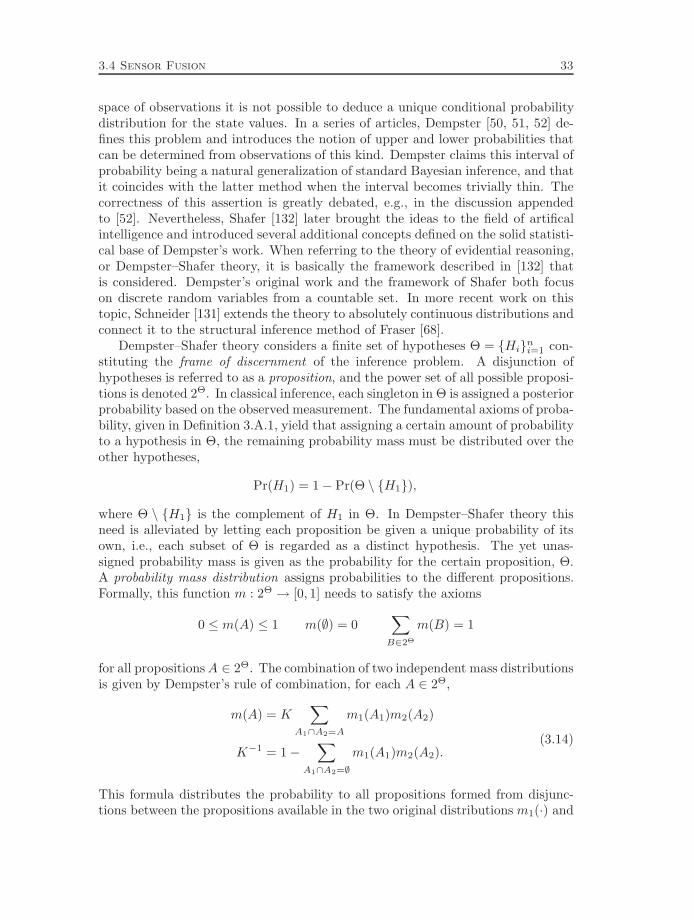
3.4 Sensor Fusion 33
space of observations it is not possible to deduce a unique conditional probabilitydistribution for the state values. In a series of articles, Dempster [50, 51, 52] de-fines this problem and introduces the notion of upper and lower probabilities thatcan be determined from observations of this kind. Dempster claims this interval ofprobability being a natural generalization of standard Bayesian inference, and thatit coincides with the latter method when the interval becomes trivially thin. Thecorrectness of this assertion is greatly debated, e.g., in the discussion appendedto [52]. Nevertheless, Shafer [132] later brought the ideas to the field of artificalintelligence and introduced several additional concepts defined on the solid statisti-cal base of Dempster’s work. When referring to the theory of evidential reasoning,or Dempster–Shafer theory, it is basically the framework described in [132] thatis considered. Dempster’s original work and the framework of Shafer both focuson discrete random variables from a countable set. In more recent work on thistopic, Schneider [131] extends the theory to absolutely continuous distributions andconnect it to the structural inference method of Fraser [68].
Dempster–Shafer theory considers a finite set of hypotheses Θ = Hini=1 con-stituting the frame of discernment of the inference problem. A disjunction ofhypotheses is referred to as a proposition, and the power set of all possible proposi-tions is denoted 2Θ. In classical inference, each singleton in Θ is assigned a posteriorprobability based on the observed measurement. The fundamental axioms of proba-bility, given in Definition 3.A.1, yield that assigning a certain amount of probabilityto a hypothesis in Θ, the remaining probability mass must be distributed over theother hypotheses,
Pr(H1) = 1− Pr(Θ \ H1),
where Θ \ H1 is the complement of H1 in Θ. In Dempster–Shafer theory thisneed is alleviated by letting each proposition be given a unique probability of itsown, i.e., each subset of Θ is regarded as a distinct hypothesis. The yet unas-signed probability mass is given as the probability for the certain proposition, Θ.A probability mass distribution assigns probabilities to the different propositions.Formally, this function m : 2Θ → [0, 1] needs to satisfy the axioms
0 ≤ m(A) ≤ 1 m(∅) = 0∑B∈2Θ
m(B) = 1
for all propositionsA ∈ 2Θ. The combination of two independent mass distributionsis given by Dempster’s rule of combination, for each A ∈ 2Θ,
m(A) = K∑
A1∩A2=A
m1(A1)m2(A2)
K−1 = 1−∑
A1∩A2=∅m1(A1)m2(A2).
(3.14)
This formula distributes the probability to all propositions formed from disjunc-tions between the propositions available in the two original distributions m1(·) and
34 Bayesian Estimation
m2(·). A probability interval is computed from the combined probability mass.The support of a proposition A is defined as
Sp(A) =∑
B:A⊆Bm(B),
which can be interpreted as all probability in m(·), in some sense pointing at A.The support is the upper limit of the probability interval for a proposition. Thelower limit, known as the plausibility of the proposition, is defined as the lack ofsupport for its negation, i.e., Pl(A) = 1− Sp(¬A).
A justification of the inference rule (3.14) based on probability theory was pre-sented in the original work of Dempster [51]. Generally, the combination rule (3.14)follows straightforwardly by regarding each proposition as a unique hypothesis andapplying Bayes’ rule. This connection, however, is not emphasized in work onDempster–Shafer theory presented, e.g., in the senor fusion or artifical intelligenceliterature. It is even not emphasized in the original work of Dempster. Instead,initiated by the book of Shafer [132], a number of less rigorously verified extensionshave been developed. Most of these are not theoretically justified from a statisticalpoint of view.
The key feature of the Dempster–Shafer approach is the ability of introduc-ing ignorance into the posterior probabilities. This effect is obtained by assigningprobability to the certain event Θ. In classical inference, ignorance is handledby spreading the remaining probability equally over the possible hypotheses. Thespokesmen of Dempster–Shafer theory claim that such an approach sometimescan yield misleading conclusions. Application of Dempster-Shafer theory is of-ten directed towards identification of object properties, by utilizing observationson several levels of abstraction. Examples involve identification of aircraft typeand class in target tracking systems [29, 35, 67] and object recognition in mo-bile robotic navigation [107]. The general conclusion drawn in all these referencesis that Dempster–Shafer not necessarily yields better performance than classicalprobabilistic inference. Even if the Dempster–Shafer framework might seem bettersuited for these problems, it is rather complex to implement and in recursive con-stellations it will often yield slower convergence towards a stationary result thanclassical inference [29, 35]. Arguments against Bayesian inference, on the basis ofits demand for priors, have also been raised when comparing classical Bayesian in-ference with Dempster–Shafer type information fusion. However, it is rather easyto realize that both methods can utilize or ignore prior information as desired.
3.5 Recursive Estimation
Many applications of estimation theory tackle the problem of recursively deter-mining, or tracking, parameters given measurements. Either the parameters admitsome dynamical properties that make them change with time, and/or the estimateof the parameters is needed on-line demanding the information about the parame-ters to be updated with each new measurement. Examples of applications that fall

3.5 Recursive Estimation 35
into this category are target tracking systems, used in both civilian and militaryaviation, and for naval applications. Here, the complete kinematic state consistingof position, velocity and possibly acceleration of the target is sought by passive oractive position measurements. Other examples of recursive estimation are all typesof navigation applications ranging from global aircraft and ship navigation down toautonomous robot navigation. Recursive estimation is also applied in adaptive con-trol, where the parameters of a dynamical system working in closed loop are trackedusing measurements of system input and output. One may also resort to recursiveestimation in off-line applications with large amounts of data. In cases when thejoint density p(x, y) is very complicated due to the size of the measurement vectory, treating the problem recursively can yield a reasonable tradeoff between com-putational complexity and performance. Detailed surveys over nonlinear recursiveestimation can be found in Sorenson [137], and Kulhavy [106].
In recursive estimation problems the parameters are usually referred to as statesof the system and they may change with time. Let xt denote the state at time t,where we always let the time index t ∈ N independently of the actual time evolved.This will allow for unequally spaced time steps within the same framework whilekeeping the notation streamlined. Uniformly spaced time intervals will howeverbe assumed unless stated differently. The notation T will be used for the fixedsampling interval.
If a correct modeling of the problem has been performed, the states xt arechosen such that they describe everything about the system at the present time.Hence, conditioned on the present state no additional information about the futurestates should be available in past observations. This Markovian property of thesystem states is fundamental to recursive estimation. The following propositiondefines the type of recursive estimation problems that we study in this thesis.
Proposition 3.2A recursive estimation problem is an estimation problem where the states evolve intime according to a Markov process with an initial state x0 ∼ p(x0) and transitionkernel,
p(xt+1 |xt) t = 0, 1, . . .
This transition kernel may explicitly depend on the time index. The measure-ment observed at the time instant t is conditionally independent of the previouslyobserved measurements given the current state value. The likelihood
p(yt |xt) t = 0, 1, . . . (3.15)
may explicitly depend on the time index t.
A recursive estimation problem is uniquely specified when the prior p(x0), thetransition kernel p(xt+1 |xt) and the likelihood p(yt |xt) are given. Note that thiscoincides with Proposition 3.1 since these entities define the joint density of allmeasurements and all states from time zero to time t. An example of a Bayesianformulation of a recursive estimation problem follows, its Bayesian solution is il-lustrated in the subsequent section.
36 Bayesian Estimation
Example 3.2In the bearings-only tracking problem the objective is to track the movements ofan object using measurements of the relative angle to the object. Consider, e.g., acase when the position of a ship is tracked using passive sonar measurements. Let
xt =
[x
(1)t
x(2)t
]be the north and east coordinates of the ship, and yt the bearings measurementfrom the sonar. A simple model of the inference problem with a random shipmovement is given by
xt+1 = xt + wt
yt = tan−1(x(2)t /x
(1)t ) + et
where the noises wt and et are independent, white processes with density functions
p(wt) = N(wt;[00
],
[2002 0
0 2002
])p(et) = N(et; 0, 0.12)
Furthermore, let the prior knowledge about the ship position be
p(x0) = N(x0;[−20003000
],
[5002 0
0 5002
]),
and let it be independent of the noises acting on the system. It is a recursiveestimation problem to determine the ship position xt, given all collected data frominitial time to present. A model specification in accordance with Proposition 3.2is given by
p(xt+1 |xt) = N(xt+1;xt,
[2002 0
0 2002
])p(yt |xt) = N
(yt; tan−1(x(2)
t /x(1)t ), 0.12
)and p(x0) given above.
3.5.1 Conceptual Solution
All recursive estimation problems that can be expressed in the form of Proposi-tion 3.2 have a common conceptual solution consisting of a recursive propagationof the conditional density. The stacked vector of the complete measurement historyat time t has length (t+ 1)p and is denoted by
Yt =
y0
y1
...yt
, and generally Ys:t =
ysys+1
...yt

3.5 Recursive Estimation 37
for any s < t. This notation will be adopted generally for stacked vectors of randomprocesses. Applying Bayes’ rule (3.1) to the last element of the measurement vectorYt yields
p(xt |Yt) =p(yt |xt,Yt−1)p(xt |Yt−1)
p(yt |Yt−1)
=p(yt |xt)p(xt |Yt−1)
p(yt |Yt−1)(3.16)
since, by (3.15), we assume that the observation yt is conditionally independent ofprevious measurements given the state xt. The expression (3.16) is referred to asthe measurement update in the Bayesian recursion. As in (3.1) the denominatorcan be expressed through the law of total probability, i.e., by marginalization.
The effect of a time step is obtained by observing that
p(xt+1, xt |Yt) = p(xt+1 |xt,Yt) p(xt |Yt)= p(xt+1 |xt) p(xt |Yt)
which follows from the assumption that the process xt is Markovian, and thatxt+1 is independent of Yt when xt is given. Integrating both sides with respect toxt yields the time update equation
p(xt+1 |Yt) =∫Rnp(xt+1 |xt)p(xt |Yt) dxt. (3.17)
This relation is also referred to as the Chapman-Kolmogorov equation [94]. Af-ter (3.17) has been evaluated, the time index can be increased and the effect of anew measurement incorporated as in (3.16). To summarize, a recursive propagationof the posterior filter density of the states given the measurements is obtained.
Theorem 3.3A recursive estimation problem of the form in Proposition 3.2 has a recursiveBayesian solution
p(xt |Yt) =p(yt |xt)p(xt |Yt−1)
p(yt |Yt−1)
p(xt+1 |Yt) =∫Rnp(xt+1 |xt)p(xt |Yt) dxt
t = 0, 1, . . .
where
p(yt |Yt−1) =∫Rnp(yt |xt)p(xt |Yt−1) dxt
and the recursion is initiated by p(x0 |Y−1) = p(x0).

38 Bayesian Estimation
Commonly used point estimates derived from the posterior density are
xMSt|t =
∫Rnxtp(xt |Yt) dxt
xMAPt|t = arg max
xtp(xt |Yt),
compare to (3.6) and (3.7). Their respective estimation error covariance is
Pt|t =∫Rn
(x− x)(x− x)T p(xt |Yt) dxt.
One often distinguishes between the problems of filtering and prediction in recursiveestimation. The solution to the filtering problem is given in Theorem 3.3 while thesolution to the prediction problem is given by performing extra time updates (3.17).
As noted in the title of this subsection, the recursive propagation of the posteriordensity in Theorem 3.3 is only a conceptual solution. In general, the multidimen-sional integrals in Theorem 3.3 and in the calculation of estimates and the errorcovariances above have no explicit analytical solutions. Only when all these inte-grals have analytical solutions for any admissible measurement sequence Yt and forall times t can the recursive Bayesian solution be solved analytically. The posteriordensity is then said to be parameterized by a finite dimensional sufficient statis-tic. For general models with nonlinear and non-Gaussian elements, this happensonly very rarely. Hence, in a practical application of Theorem 3.3 one is forced towork with some approximate description of the posterior filter density. The formatof this approximation should be well-suited for propagation through Theorem 3.3and for calculation of the chosen estimate and its error covariance. The choice ofnumerical approximation will be handled in detail in Chapter 5.
We conclude this subsection with an illustration of the Bayesian solution to acommon target tracking problem.
Example 3.3 (Continued from Example 3.2)Inserting the model of the bearings-only tracking problem from Example 3.2 intothe Bayesian solution in Theorem 3.3 yields
p(xt |Yt) ∝ N(yt; tan−1(x(2)
t /x(1)t ), 0.12
)p(xt |Yt−1)
p(xt+1 |Yt) =∫R2
N(xt+1;xt,
[2002 0
0 2002
])p(xt |Yt) dxt
initiated by
p(x0 |Y−1) = N(x0;[−20003000
],
[5002 0
0 5002
]).
Figure 3.1 shows a simulation with three snapshots of a numerical approximationto the conditional density. The figure shows numerical approximations to the priorp(x0 |Y−1), and the posterior p(xt |Yt) at two stages of the recursion. Naturally,the posterior density is narrow seen from the platform but widespread along theline-of-sight between ship and platform.
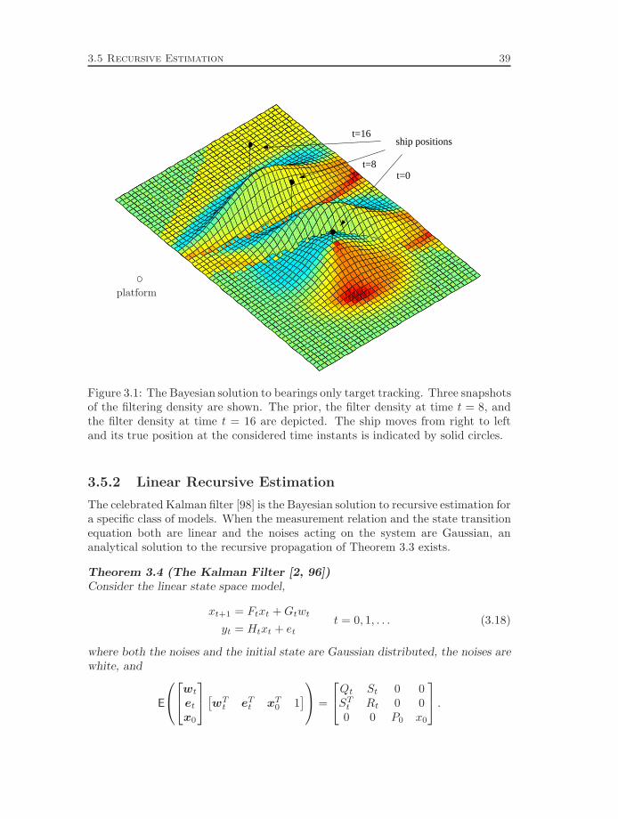
3.5 Recursive Estimation 39
ship positions
t=0 t=8
t=16
platform
Figure 3.1: The Bayesian solution to bearings only target tracking. Three snapshotsof the filtering density are shown. The prior, the filter density at time t = 8, andthe filter density at time t = 16 are depicted. The ship moves from right to leftand its true position at the considered time instants is indicated by solid circles.
3.5.2 Linear Recursive Estimation
The celebrated Kalman filter [98] is the Bayesian solution to recursive estimation fora specific class of models. When the measurement relation and the state transitionequation both are linear and the noises acting on the system are Gaussian, ananalytical solution to the recursive propagation of Theorem 3.3 exists.
Theorem 3.4 (The Kalman Filter [2, 96])Consider the linear state space model,
xt+1 = Ftxt +Gtwt
yt = Htxt + ett = 0, 1, . . . (3.18)
where both the noises and the initial state are Gaussian distributed, the noises arewhite, and
E
wt
etx0
[wTt eTt xT0 1
] =
Qt St 0 0STt Rt 0 00 0 P0 x0
.

40 Bayesian Estimation
The conditional density for the one-step ahead prediction problem, p(xt |Yt−1), isGaussian. Initiated by x0 = x0, the mean obeys the recursion
xt+1 = Ftxt +Kt(yt −Htxt),
where Kt = (FtPtHTt +GtSt)(Rt +HtPtH
Tt )−1 and the posterior covariance is
Pt+1 = FtPtFTt −Kt(Rt +HtPtH
Tt )KT
t +GtQtGTt
initiated by P0.
Proof A proof of the statement above along with comprehensive presentations regardingall aspects of Kalman filtering can be found in, e.g., [2, 96].
For the linear and Gaussian model class described above, Theorem 3.1 yields thatthe posterior distribution is Gaussian. Hence, a sufficient statistic consists of themean vector and the covariance matrix of this Gaussian conditional density. It isthese parameters that are given by the analytical solution to the Bayesian recursiveestimation problem in the theorem above. Due to the properties of the Gaussiandensity, the recursively updated parameters also coincide with the mean-squareestimate and its error covariance for the linear Gaussian model class. The Kalmanfilter has several interpretations apart from being a Bayesian solution to a certainclass of models, see [2, 96] for a thorough presentation of linear estimation theory.
3.5.3 Nonlinear Recursive Estimation
Most real-world problems have elements of nonlinearity, non-Gaussianity and non-stationarity. For this large class of practical problems it is not possible to deriveexact closed form solutions for the estimators and estimation error covariances. Themost common approach to circumvent this problem has been to resort to modelsimplifications and approximations which inevitably will lead to performance degra-dations. In critical situations where one cannot compromise the accuracy of theresult, the only way to solve these inference problems is by numerical approxima-tion techniques. A few notable exceptions of non-standard models with exact finitedimensional solutions exist, see, e.g., [65, 105]. For practical nonlinear estimation,approximative solutions must in general be considered. These approximations canbe categorized into two groups, either the underlying model of the problem is sim-plified so that an analytical solution is obtained, or an approximative descriptionof the posterior distribution itself is determined.
Local model approximations
The approach to locally approximate the nonlinear model is the most frequentlyused practical technique for nonlinear recursive estimation. The nonlinear modelequations are expanded into a Taylor series around a point estimate of the states.A model of the form (3.18) is obtained by inserting the estimate obtained from

3.5 Recursive Estimation 41
the last iteration of the algorithm, and approximating the distributions of noisesacting on this linearized model with Gaussian distributions. The system matricesof this linear time dependent model will explicitly depend on the estimate that thelinearization is performed around. Disregarding this dependence, the Kalman filtercan be applied directly to this linearized time dependent model. This scheme isusually labeled the Extended Kalman Filter (EKF) [2, 94]. Several applications ofEKF techniques to nonlinear estimation problems can be found in Sorenson [136].
The EKF approach yields a nonlinear estimation filter with very modest com-putational requirements that is frequently applied in practical recursive nonlinearestimation such as target tracking, navigation, and robotics. However, there aresome well known disadvantages with this linearization technique. It often happensthat the estimation error Pt, calculated by the algorithm, becomes inconsistentwith the true estimation error. Usually, the filter underestimates this error result-ing in a reduction of the filter gain and an insensitivity to new measurements. Thiseffect is labeled the divergence problem of the EKF. The situation usually arises asa result of linearization errors when the local approximation ceases to hold. Apartfrom manually keeping the filter gain above a certain level, several generalizationsthat deal with the divergence problem have been proposed. These include meth-ods for higher order approximation schemes and the iterated version of the EKF.Jazwinski [94] gives a thorough treatment of these topics.
Another sort of model approximation is obtained by letting the state vector belimited to a finite number of values. In this case the conditional density recursioncan be solved by approximately determining the conditional probability for eachcandidate state value using numerical integration methods. This type of model withdiscrete valued states is often referred to as a Hidden Markov Model (HMM). Acomprehensive presentation of HMMs, containing results regarding both estimationand control, can be found in Elliott et al. [63], and a tutorial over HMMs is givenby Rabiner [125].
Global approximation of the posterior density
The local linearization technique of the EKF fails to hold when the nonlinearityof the model is substantial, the initial estimate is bad or the noises acting on themodel are far from Gaussian distributed. A global approximation is obtained bykeeping the original nonlinear model but instead solving the Bayesian recursion ofTheorem 3.3 approximately. There are two common approaches to global approx-imation of the Bayesian solution. Either the posterior density is parameterized ina finite number of parameters that are inserted into the Bayesian recursion andapproximately updated with each iteration, or the integrals in the recursion aredirectly attacked by numerical integration methods. Both these approaches resultin similar globally approximate Bayesian filters. With no linearization errors in-troduced, these methods promise a solution closer to the optimal one. Contrary tothe EKF technique, these filters may, e.g., handle multi-modal conditional densitieswithout any further modifications. However, this is usually obtained at the priceof a substantially higher computational burden.
42 Bayesian Estimation
Numerical integration methods based on grid approximations of the posteriordensity will be presented in more detail in Chapter 5. In many cases, the result-ing algorithms of numerical integration will be rather similar to the approach ofapproximating the conditional density. Generally, practical on-line estimation is afunction approximation problem under the constraints that an efficient and reliableupdate of the function expansion through the Bayesian recursion is possible. Themeasurement and time updates consist of multiplications and convolutions betweenprobability density functions. From the analytical solution of the linear Gaussianmodel, it is known that multiplying and convolving Gaussian distributions willgenerate new Gaussian distributions. A reasonable approximative expansion of theposterior is therefore obtained by a weighted sum of Gaussian distributions,
p(xt |Yt−1) ≈N∑i=1
γi N(xt;µi,Σi). (3.19)
This is utilized in the Gaussian sum estimation techniques introduced by Alspachand Sorenson [1], Sorenson and Alspach [138]. Through the measurement updatemultiplication, the number of terms in the approximating sum (3.19) will in generalincrease at each iteration. In [1, 138] it is therefore suggested that terms with smallweights should be neglected and terms that are close should be combined into asingle term at each iteration of the algorithm.
Another expansion that lends itself to the nonlinear estimation problem is thepoint-mass approach, originally suggested by Bucy and Senne [34]. In the point-mass approach the posterior is approximated by a set of point values on a movinggrid
p(xt |Yt) ≈N∑i=1
piδ(xt − xit).
With this approach, the integrals will be replaced by summations that can besuitably truncated over finite intervals. The point-mass approximation has beengeneralized to piecewise constant approximations by Kramer [102], Kramer andSorenson [104]. This approach to nonlinear filtering was developed during theearly 1970’s. At this time, the main concern about the practical applicabilityof these techniques was the problem of storing the comparatively large number ofgrid points. Due to this constraining limitation, research focused on more advancedinterpolation techniques that could produce the same results with fewer grid points.The spline filters of de Figueiredo and Jan [47] and Youssef [155] were developedwith this in mind. The more advanced interpolation schemes in general suffer froma more complicated description of the grid nodes. The propagation of the gridintroduces extra overhead computations that, to a large extent, compensate forthe reduction of the number of interpolation functions. A thorough background tothe development of global approximation methods in nonlinear estimation with anemphasis on point-mass approximations is presented in [137]. Lately, the point-mass approaches have had a minor revival due to the rapid increase in desktop

3.5 Recursive Estimation 43
computer memory size and floating point computational performance. Simandland Kralovec [133] give some general guidelines towards choosing the grid resolutionand support.
A somewhat different approach to approximation of the posterior distribution istaken by Kulhavy [106]. From the empirical density of the observations, a paramet-ric posterior distribution from an exponential family is determined using convex op-timization methods. This optimization can be posed such that each new measure-ment is added recursively and an on-line implementation is thus possible. Kulhavyonly considers inference of nonrandom parameters but introduces the possibility oftracking time-varying parameters using forgetting factor techniques. Applicationsto several recursive estimation problems and to adaptive control problems are givenin [106].
3.5.4 Continuous Time Filtering
Above, and throughout this thesis, we study the recursive estimation problem indiscrete time only. Hence, the Markovian transitions of the states is assumed toevolve in discrete steps and the measurements are obtained at discrete time in-stants. One can argue that the class of purely discrete time models, althoughpossibly nonlinear, is too restrictive for practical application. Often, real worldphenomena evolve in continuous time while measurements are collected at discretetime instants. Consider, e.g., the target tracking problem where the position andvelocity of an aircraft target change continuously in time while the radar measure-ments are obtained periodically, when the target is illuminated by the rotatingradar antenna.
With continuous time state evolution, the Chapman-Kolmogorov equation (3.17)will turn into a partial differential equation, often referred to as the Kolmogorovforward equation or the Fokker-Plank equation [94]. This nonlinear partial differ-ential equation has been studied extensively in the field of optimal filtering. Apartfrom the obvious linear Gaussian case, analytical solutions to the Fokker-Plankequation have only been found in rare cases [13, 43]. For general nonlinear andnon-Gaussian models, EKF linearization techniques can be applied similarly tothe discrete time case. The counterpart to the numerical integration approach ofdiscrete time filtering is numerical solution of the nonlinear Fokker-Plank partialdifferential equation. A general adaptive grid method for this problem has beendeveloped by Cai et al. [36]. The techniques are similar to the nonlinear integra-tion methods for discrete time filtering and in general very time consuming andapplication specific.
From almost any continuous time evolution, a purely discrete time model can beobtained by performing several small time update steps between each measurementupdate. For this reason, we will solely consider discrete time estimation problemsand for simplicity that only one time update is needed between each measurementupdate. A thorough treatment of discrete and continuous time nonlinear filter-ing and estimation as well as hybrid problems with, e.g., continuous time stateevolution and discrete time measurements, is given by Jazwinski [94].
44 Bayesian Estimation
3.6 Summary
Many practical problems in signal processing can be described accurately by anunderlying statistical model of the problem. In this context, the Bayesian approachto statistical inference gives a natural framework where information given as priorknowledge as well as information in observations are considered. Both parametersand observations are regarded as random variables and inference is performed byconditioning through Bayes’ rule.
The posterior density p(x | y) summarizes the information gained after observingthe experimental outcome y. The mean of this function xMS is an estimate thatminimizes the Bayesian risk for a large class of cost functions. The error covarianceof xMS is equal to the covariance of the random variable x | y and is useful whencomparison or combination with other estimates should be performed.
The expressions for the normalizing factor of the posterior p(x | y), the esti-mate and estimation error covariance, all involve multidimensional integrals oroptimizations. Unfortunately, it is only in certain special cases these integrals andoptimizations have analytical solutions. In a recursive setting the Bayesian solutionconsists of sequentially updating the posterior density with each new observationand with time. This posterior can only rarely be parameterized using a finite dimen-sional sufficient statistic which may be sequentially updated analytically. Practicalrecursive Bayesian estimation therefore demands numerical solutions to high di-mensional complex integrations or optimizations with respect to the parameters.In addition to solving these integration problems, the posterior density itself mustbe approximately described in a way that lends itself to approximate propagationthrough the conceptual Bayesian solution.

Appendix
3.A Foundational Concepts of Probability Theory
This appendix summarizes the basic concepts of probability theory, from Kol-mogorov’s definition of probability to conditional probability density functions andBayes’ law. It also serves to settle the notation used in the thesis. The appendixrelies on several texts, the main reference is [120]. The presentation herein is by nomeans complete or comprehensive. Thorough treatments of the topics presented inthis appendix with complete proofs, enlightening discussions and several additionalconcepts can be found in either of [40, 109, 120].
3.A.1 Probability Theory
The basic concepts of probability theory are the event space Ω, which consists ofall possible outcomes of an experiment, and events which are subsets of Ω. Theevent space Ω is also referred to as the certain event, while the empty set, ∅, is theimpossible event. Events that are singletons are sometimes denoted ω.
Definition 3.A.1 (Axiomatic definition of probability)To each event A we assign the number Pr(A) which we call the probability of theevent A. The probability is chosen to satisfy the following four axioms:
1. Pr(A) ≥ 0
2. Pr(Ω) = 1
3. If A ∩B = ∅, then Pr(A ∪B) = Pr(A) + Pr(B).
4. If Ai ∩Aj = ∅ for i 6= j, then Pr(∪∞i=1Ai) =∑∞
i=1 Pr(Ai)
All statistical inference is based on the concept of conditional probabilities. Aconditional probability describes what effect knowing a certain event has on theprobabilities of other, related, events.
45

46 Bayesian Estimation
Definition 3.A.2The conditional probability of an event A given an event M of nonzero probabilityPr(M) > 0 is defined as the ratio
Pr(A |M) =Pr(A ∩M)
Pr(M)
It is readily possible to verify that a conditional probability is a probability inaccordance with the axioms of Definition 3.A.1. From this we can deduce that theprobability of every event can be written as a sum of conditional probabilities.
Theorem 3.A.5 (Total probability theorem)Let A1, . . . ,An be a partition of Ω and let B be an arbitrary event, then
Pr(B) = Pr(B |A1) Pr(A1) + · · ·+ Pr(B |An) Pr(An)
Combining Definition 3.A.2 and Theorem 3.A.5 yields the following famous formulafor conditional probability, originally due to Bayes [9] in 1763.
Theorem 3.A.6 (Bayes’ theorem)Let A1, . . . ,An be a partition of Ω and let B and M be two events, then
Pr(M |B) =Pr(B |M) Pr(M)
Pr(B |A1) Pr(A1) + · · ·+ Pr(B |An) Pr(An)
3.A.2 Random Variables
A random variable is a real valued function with domain Ω, the set of all possibleexperimental outcomes. For every outcome ω we assign a real number x(ω). We willoften omit the explicit dependency on the event ω and write the random variable asa bold character x. Due to the frequent use of stochastic variables in this thesis wewill even alleviate the bold character notation when no risk for ambiguity exists.The set x ≤ x is a set in the event space, a subset of Ω consisting of all outcomesω such that x(ω) ≤ x. The distribution function of x is the function
Px(x) = Pr(x ≤ x),
and the density function is the derivative of the distribution function
px(x) =dP (x)dx
.
When no risk of ambiguity exists, we will omit the subindex in the notation Px(x)and px(x), and simply write P (x) and p(x).
Definition 3.A.2 of conditional probability is straightforwardly extended to dis-tribution functions.

3.A Foundational Concepts of Probability Theory 47
Definition 3.A.3 (Conditional distribution)The conditional distribution of a random variable x given an event M of nonzeroprobability Pr(M) > 0 is
P (x |M) = Pr(x ≤ x |M) =Pr(x ≤ x,M)
Pr(M).
The event x ≤ x,M is the event consisting of all outcomes ω such that x(ω) ≤ xand ω ∈M.
The conditional density is the derivative of P (x |M),
p(x |M) =dP (x |M)
dx= lim
∆x→0
P (x ≤ x ≤ x+ ∆x |M)∆x
The conditional probability of the event A given an event of zero probability, likex = x, is defined through the limit
Pr(A |x = x) M= lim∆x→0
Pr(A |x ≤ x ≤ x+ ∆x). (3.A.20)
The total probability theorem, Theorem 3.A.5, for conditional events of zero prob-ability can then be expressed as an infinite sum over the limits in (3.A.20). Hence,the probability of any event A can be written
Pr(A) =∫ ∞−∞
Pr(A |x = x)p(x) dx.
The conditional density of x given the event A is
p(x |A) =Pr(A |x = x) p(x)
Pr(A). (3.A.21)
So far we have considered events and real scalar random variables. The exten-sion to vector valued random variables follows conceptually by looking at pairs ofscalar variables. The distribution and density functions extend naturally as
P (x, y) = Pr(x ≤ x,y ≤ y)
p(x, y) =∂2P (x, y)∂x ∂y
.
These functions are occasionally given the prefix joint distribution and densityfunction, respectively. The definition of conditional distribution and density appliesto pairs of random variables as well
P (x, y |M) =Pr(x ≤ x,y ≤ y,M)
Pr(M)
p(x, y |M) =∂2P (x, y |M)
∂x ∂y(3.A.22)

48 Bayesian Estimation
As in Definition 3.A.3, it is assumed that Pr(M) > 0. The conditional density of arandom variable y, assuming the value of some other random variable x is known,is frequently used in statistical inference. This density cannot be derived directlyfrom (3.A.22) due to the fact that the event x = x generally has zero probability.Instead, this density is defined through the limit
p(y |x = x) = lim∆x→0
p(y |x < x ≤ x+ ∆x) =p(x, y)p(y)
. (3.A.23)
When no risk of ambiguity exists, the shorter notation p(y |x) will be used inliu of the somewhat cumbersome notation p(y |x = x). Combining (3.A.23)with (3.A.21) yields the most common version of Bayes’ theorem.
Theorem 3.A.7 (Bayes’ theorem and total probability)The conditional density can be written
p(x | y) =p(y |x) p(x)
p(y)(3.A.24)
where the normalizing constant in the denominator can be expressed using the lawof total probability
p(y) =∫Rnp(y |x)p(x) dx.
The function p(y |x) is labeled the likelihood while the density function of theparameters p(x) is called the prior . Using the total probability theorem it is worthnoting that Bayes’ law (3.A.24) can be expressed solely using the joint density ofx and y,
p(x | y) =p(y, x)∫
Rn p(y, x) dx.
Since the conditional density is the fundamental solution to the inference problem,it follows that the joint density is the only description needed for doing statisticalinference.

4
Cramer-Rao Bounds
The posterior filter density of most nonlinear recursive estimation problems cannotbe described analytically by a finite number of parameters. Several examples ofsuboptimal algorithms for practical nonlinear recursive estimation have thereforeappeared in the literature. Generally, these procedures approximate either the es-timation model or the description of the posterior distribution. These inevitableapproximations may seriously degrade the estimation performance compared tothe results obtained if the posterior filter density was known exactly. It is of greatpractical interest to quantify this performance degradation, and measure the effectof the introduced approximations. A benchmark simulation evaluation against theoptimal solution is not an option since it would require infinite computing powerand unlimited memory resources to run the optimal algorithm. However, even if theoptimal solution is intractable, the performance of the optimal algorithm may veryoften be computed with limited resources. The estimation error obtained with anoptimal algorithm depends only on fundamental properties of the model, e.g., sig-nal to noise levels and prior assumptions on the sought parameters. Characteristicsof the optimal estimation error define lower limits on the performance that can beachieved using any approximative implementation. The characteristics of the sub-optimal estimation error are revealed in simulation studies using the implementedprocedure. The discrepancy from the lower bound gives an indication of the effectof the approximations introduced in the implemented algorithm. A relative com-parison between the suboptimal and the optimal algorithms is therefore possible
49

50 Cramer-Rao Bounds
even if it is intractable to implement the optimal solution. A lower bound on someproperty of the estimation error is convenient when evaluating implemented sub-optimal procedures, but can also be used to quantify the fundamental performancelevel that can be reached for the currently studied estimation problem.
In this chapter we focus on the fundamental Cramer-Rao bound which sets alower limit on the mean square estimation error. The bound states that the dif-ference between the expected mean square error correlation matrix and a matrixdetermined by the model of the estimation problem, should always be positivesemidefinite. The parametric and the Bayesian viewpoints on estimation give twodifferent kinds of Cramer-Rao bounds. These bounds, known as parametric andposterior Cramer-Rao bounds respectively, are reviewed in Section 4.1. In Sec-tion 4.2, we review some results on Cramer-Rao bounds for recursive estimation,and present the class of nonlinear state space estimation models that is consideredin this work. The subsequent section presents compact expressions for the para-metric Cramer-Rao bound for general filtering and prediction. The smoothing caseis also handled, in a somewhat rudimentary fashion. The recursive formulas for theCramer-Rao bound hold true for general nonlinear and non-Gaussian models andrequire limited computational efforts and memory resources. Similar expressionsare presented using the posterior bound in Section 4.4. Without restrictions thatguarantee non-singularities in the state evolution process, the computations andstorage requirements for the posterior Cramer-Rao bound for recursive estimationwill increase linearly with time. The class of estimation problems for which theposterior Cramer-Rao bound can be computed with limited effort still includesgeneral nonlinear models with possibly non-Gaussian noises. In Section 4.5, wepresent some suggestions to the practical application of the Cramer-Rao bounds.The utilization of both the parametric and the posterior Cramer-Rao bound is alsoexemplified by the terrain navigation application in Chapter 7. A summary of theresults and some conclusive remarks are finally given at the end of this chapter.
4.1 Review over Cramer-Rao Bounds
In this section, we review the Cramer-Rao bound for the generic estimation problemdiscussed in Section 3.2. The sought parameters are assembled in an n-dimensionalvector x and the observations are given as a p-dimensional vector y. For randomparameters, the estimation relies on the Bayesian paradigm and the problem isuniquely specified by the joint density p(x, y) = p(y |x)p(x). For nonrandom pa-rameters, it is the likelihood p(y |x) that alone defines the estimation problem.
For sake of completeness, the bounds reviewed in this section are presented withderivations from first principles. The technical details of the proofs are summarizedin Appendix 4.B. The fact that we deliver complete derivations does not mean thatwe claim originality of all the results presented. The main results of this reviewcan be found in any textbook on estimation theory. For a thorough treatment ofthe results in this section we refer to the excellent, and now classical, monographof Van Trees [151].

4.1 Review over Cramer-Rao Bounds 51
Commonly, the Cramer-Rao bound for multiple parameter estimation is derivedas an extension from the scalar case. Contrary to, e.g., Van Trees [151], we chooseto present the general bounds for vector valued estimation directly. In addition,we introduce a slight generalization of the classical bounds. This modification isutilized in the application of the bounds to the recursive estimation problem. Itallows us to derive expressions for the Cramer-Rao bound to a general class of statespace estimation problems.
4.1.1 Estimator Performance
Consider the generic statistical inference problem of estimating an n-dimensionalparameter x based on a p-dimensional observation vector y. The fundamentalCramer-Rao bound sets a lower limit on the mean square estimation error of anyestimator x(y). The bound applies to all estimators under certain conditions onthe estimator bias, which is defined as the expected systematic error it producesaveraged over all measurements.
Definition 4.1The bias of an estimator x(y) is the expected error,
B(x) M=∫Rp
(x(y)− x)p(y |x) dy.
In parametric estimation, the bias vector is a function of the unknown but fixedtrue parameter x = x?. In the Bayesian framework, it is a random vector definedby the function B(·), and the prior distribution p(x). Depending on the propertiesof the bias vector, the estimators are grouped into three different classes.
Unbiased When the bias B(x) = 0 for all x, the estimator is unbiased . On theaverage, the estimate equals the sought parameter.
Known bias When the bias is nonzero but independent of the parameter B(x) =B, the estimator is said to have a known bias . An unbiased estimator isstraightforwardly obtained by subtracting the known bias from the estimate.
Unknown bias In the general case, B(x) is a function of the unknown param-eter x and the estimator is said to have an unknown bias . Since the biasis a function of the unknown parameter, it cannot be subtracted from theestimate.
An unbiased estimator for the nonrandom parameter x has an estimation errorcovariance given by
C = Cov(x(y)− x) = E((x(y)− x)(x(y)− x)T
).
In parametric estimation the expectation is performed over the only stochasticvariable, viz. y, using the parameterized density p(y |x). Given any unbiased es-timator defined for a parametric estimation problem, the Cramer-Rao bound for
52 Cramer-Rao Bounds
this problem is a matrix P of the same dimension as the estimator error covarianceC that satisfies
C − P ≥ 0. (4.1)
The inequality in (4.1) means that the left hand side is positive semidefinite. Inthe random parameter case, it turns out that the bias has less importance and thatthe estimation error correlation matrix, or mean square error matrix,
C = E((x(y)− x)(x(y)− x)T
)= Cov(x(y)− x) + E(B(x)) E
(BT (x)
)satisfies the Cramer-Rao inequality (4.1), given only minor assumptions on theestimator bias. In the random case, the expectation is over both x and y, usingthe joint density p(x, y).
The Cramer-Rao bound P is uniquely determined by the estimation model.In the case of fixed nonrandom parameters, P depends on the likelihood and theunknown fixed parameter. In the Bayesian random case, P depends on the jointdensity. Proof of (4.1) and expressions for P in both the case of parametric andof random estimation follow in the two subsequent sections. The material of thesetwo subsections have mainly been collected from [151]. An alternative presentationonly covering the parametric case is given by Scharf [130]. However, the Cramer-Rao bounds presented below are somewhat generalized versions of the ones foundin [151]. We introduce the ability to distinguish between the parameter vector thatwe are interested in estimating, x, and the vector z that affects the estimationmodel. This makes it possible to handle cases when the prior density of x issingular, i.e., involves Dirac delta measures.
The sequel of this chapter involves some, rather standard, vector gradient no-tation and utilizes some basic block matrix manipulations. Appendix 4.A reviewssome of the utilized results, and settles the basic notation.
4.1.2 Nonrandom Parameters
When the parameters are regarded as unknown but fixed, they define a parameter-ization of all admissible probability density functions for the observations, p(y |x).The parametric Cramer-Rao bound depends on this likelihood and on the trueunknown parameter, denoted by x?.
The score function is the gradient of the logarithm of the likelihood
∇x log p(y |x).
In maximum likelihood estimation, this function returns a vector valued score giventhe observation y and a candidate parameter vector x. Scores close to zero are goodscores since they indicate that x is close to a local optimum of p(y |x). Regardingp(y |x) as a positive function of x,
∇x log p(y |x) =1
p(y |x)∇xp(y |x).
4.1 Review over Cramer-Rao Bounds 53
Inserting the random vector y into the score function, each candidate parametervector yields a stochastic score. The expected value of the stochastic score functionis zero since
E(∇x log p(y |x)) =∫Rp∇x(log p(y |x)) p(y |x) dy =
∫Rp∇xp(y |x) dy
= ∇x∫Rpp(y |x) dy = 0.
This implies that the correlation and covariance matrices of the score functioncoincide. The Fisher Information Matrix (FIM) is defined as this covariance matrixof the random score vector.
Definition 4.2 (The Fisher information matrix)The Fisher information matrix (FIM) is the covariance matrix of the score function
J(x) M= E(∇x log p(y |x)∇Tx log p(y |x)
)In Corollary 4.B.3 in Appendix 4.B an alternative and more compact expressionfor the FIM is given,
J(x) = E(−∆xx log p(y |x)) , (4.2)
where ∆xx is the second order partial derivative operator, see Appendix 4.A. The
FIM is a measure of the average size of the random score vector, for a givenparameter value x. We will often suppress the dependency on the parameter vectorand, when no risk of ambiguity exists, solely write J for the FIM of the currentlystudied parametric estimation problem.
In parametric estimation, the probability density function of the observations isparameterized by the sought parameter vector. The stochastic model of the obser-vation vector is uniquely defined given a parameter vector x. However, this does notimply that all elements of x or combinations of elements of x affect the stochasticproperties of the observations. The likelihood p(y |x) might be overparameterizedso that some elements of x or combinations of elements of x do not affect p(y |x),regarded as a probability density function for y. In such a case, the FIM (4.2)for the parameter vector x becomes singular. This will lead to problems whencomputing the Cramer-Rao bound. Let z ∈ Rr be an alternative parameterizationof the likelihood such that p(y | z) is a well defined density function for y givenany z ∈ Rr and the corresponding FIM is nonsingular. Hence, we let r ≤ n anddefine the possibly noninvertible coordinate transformation x = t(z). This possi-bility to distinguish between the quantity that is estimated, x, and the parametersthat directly affect the likelihood, z, is utilized in the subsequent sections whenthe bound is applied to recursive nonlinear estimation. The Cramer-Rao bound forparametric estimators x(y) given a possibly overparameterized likelihood follows.

54 Cramer-Rao Bounds
Theorem 4.1 (Parametric Cramer-Rao bound)Assume that the observation y ∈ Rp has a well defined probability density functionp(y | z) for all z ∈ Rr, and let z? denote the parameter that yields the true distri-bution of y. Moreover, let x(y) ∈ Rn be an unbiased estimator of x = t(z), and letx? = t(z?). The estimation error covariance of x(y) is bounded from below by
E((x− x?)(x− x?)T
)≥MJ−1MT
where
J = E(−∆zz log p(y | z))
z=z?and MT = ∇ztT (z)
z=z?
are matrices that depend on the true unknown parameter vector z?.
Proof A detailed proof is given in Appendix 4.B.1. In essence, the bound follows fromthe positive semi-definiteness of the covariance matrix
E
([x− x
∇z log p(y | z)
] [x− x
∇z log p(y | z)
]T)=
[C MMT J
]≥ 0.
The Schur complement of C in this block matrix gives the desired result.
Inserting the identity transformation x = t(z) = z yields the classical Cramer-Raobound which says that the estimation error covariance of any unbiased estimatoris bounded from below by the inverse of the FIM. The general bound given in The-orem 4.1, with the possibility to have a gradient matrix M 6= I, is commonly notutilized in the current literature on Cramer-Rao bounds. We believe this general-ization to be of great practical importance since the formulation above allows us toevaluate the bound in cases when the FIM is singular. A suitable reformulation ofa singular problem by parameterizing the likelihood with respect to fewer param-eters can make the FIM invertible. Theorem 4.1 yields a bound for the originallikelihood parameterization by utilizing the transformation between the differentlikelihood parameterizations. This aspect is crucial for the general Cramer-Raobounds to recursive estimation presented in the latter part of this chapter.
The general bound given in Theorem 4.1 can also be used to obtain a Cramer-Rao bound for estimators with possibly nonzero bias.
Corollary 4.1 (Biased Estimators)Consider an estimation problem defined by the likelihood p(y | z), and the fixedunknown parameter z?. Any estimator z(y) with unknown bias B(z) has a meansquare error bounded from below by
E((z − z?)(z − z?)T
)≥MJ−1MT +B(z?)BT (z?)
where
J = E(−∆zz log p(y | z))
z=z?and MT = I + ∇zBT (z)
z=z?

4.1 Review over Cramer-Rao Bounds 55
Proof Introducing the quantity x = z +B(z), the estimator x(y)M= z(y) is an unbiased
estimator of x. Hence, Theorem 4.1 yields that
E(
(x− x)(x− x)T)≥ (I +∇zBT (z))T E(−∆z
z log p(y | z))−1 (I +∇zBT (z))
and thus that
E(
(z − z)(z − z)T)≥ (I +∇zBT (z))T E(−∆z
z log p(y | z))−1 (I +∇zBT (z))
+B(z)BT (z),
after suitably inserting the true unknown parameter z?.
The Cramer-Rao bound in Theorem 4.1 depends on the true unknown parame-ter vector z?, and on the model of the problem defined by p(y | z) and the mappingt(z). Hence, the bound can typically only be computed in simulation studies, whenthe true value of the sought parameter vector is known.
4.1.3 Random Parameters
For random parameters there is no true unknown parameter value. Instead, theprior assumption on the parameter distribution determines the probability of dif-ferent parameter vectors. Like in the parametric case of the previous subsection,we allow for a possibly non-invertible mapping t : Rr → Rn between a parametervector z and the sought parameter x. The vector z is assumed to have been cho-sen such that the joint density p(z, y) is a well defined density, without singularDirac delta factors. The Cramer-Rao bound presented in the theorem below isa slight generalization of the posterior Cramer-Rao bound for multiple parameterestimation by Van Trees [151].
Theorem 4.2 (Posterior Cramer-Rao bound)Let z ∈ Rr and y ∈ Rp be two random vectors with a well defined joint densityp(z, y), and let x(y) ∈ Rn be an estimate of x = t(z). If the estimator bias
B(z) =∫Rp
(x− t(z)) p(y | z) dy
satisfies
limzi→±∞
Bj(z)p(z) = 0 for all i = 1, . . . , r and j = 1, . . . , n,
then the mean square error of the estimate is bounded from below
E((x − x)(x− x)T
)≥MJ−1MT
where
J = E(−∆zz log p(y, z)) and MT = E
(∇ztT (z)
).

56 Cramer-Rao Bounds
Proof The bound follows from the positive semidefinite correlation matrix
E
([x− x
∇z log p(z, y)
] [x− x
∇z log p(z, y)
]T)=
[C MMT J
]≥ 0.
A detailed proof is presented in Appendix 4.B.2.
Since p(z, y) = p(y | z)p(z), the “information matrix” in the posterior Cramer-Raobound can be decomposed into two matrices
J = JD + JP .
Above, JD represents the information in the observed data and JP the informationin the prior,
JD = E(−∆zz log p(y | z)) JP = E(−∆z
z log p(z)) .
Note that JD is the expectation of the parametric FIM performed under the priormeasure p(z). Alternatively, with the decomposition p(z, y) = p(z | y)p(y), theposterior bound can be written
J = E(−∆zz log p(z | y)) (4.3)
since ∆zz log p(y) = 0. Expectation is naturally performed with respect to p(z, y)
in (4.3). This expression in some sense justifies the name “posterior” Cramer-Raobound.
Contrary to the parametric case, the posterior Cramer-Rao bound can be com-puted even in real applications. Since the parameters are random there is nounknown true parameter value. Instead, in the posterior Cramer-Rao bound thematrices J and M are computed by mathematical expectation performed withrespect to the prior distribution of the parameters.
4.2 Discrete Time Nonlinear Estimation
In nonlinear recursive estimation, the primary interest lies in bounds on the filteringor prediction error. For sake of completeness, we will also determine bounds forfixed interval smoothing.
4.2.1 Background
Kerr [100] presents a general review over Cramer-Rao bounds for both continuousand discrete time nonlinear filtering. Although the continuous time case is of lesspractical interest, it has been studied in much greater detail than the discrete timecase. The Cramer-Rao bound for discrete time filtering was initially studied byBorobsky and Zakai [32]. They consider the posterior bound with the restrictionto scalar nonlinear models with additive Gaussian noise. Later, Galdos [70] ex-tended the results to the multidimensional case. A more recent generalization of
4.2 Discrete Time Nonlinear Estimation 57
the same technique is given by Doerschuk [56]. The class of models consideredin [56] are discrete time, state space representations of nonlinear autoregressiveprocesses driven by Gaussian state dependent noise having full rank covariancematrix. The approach initiated in [32] and extended in [56, 70] relies on a compar-ison between the information matrix of the nonlinear system and the informationmatrix of a suitable linear Gaussian system. According to [100], the argumenta-tion in [32] is somewhat imprecise and lacks a proper definition of the equivalencebetween the linear and nonlinear models. Some additional limitations of this ap-proach are also discussed in the general overview over lower bounds for nonlinearfiltering provided by Kerr [100]. The parametric bound has not been given thesame amount of attention in the literature as the posterior bound. A parametricbound is derived by Taylor [144] for the case of continuous time deterministic stateevolution and nonlinear discrete time measurements with additive Gaussian noise.
Lately, Tichavsky et al. [147] have derived general expressions for posteriorCramer-Rao bounds to discrete time nonlinear filtering using a different, and moregeneral, approach than developed [32]. Similar results were independently obtainedby Bergman [17]. Bounds for multidimensional state space models without anylimiting Gaussianity assumptions are derived in [147]. The approach to posteriorCramer-Rao bounds for nonlinear filtering advocated by Tichavsky et al. has servedas an inspiration for the development of a novel parametric Cramer-Rao bound forrecursive estimation presented in Section 4.3. The parametric bound can even beevaluated for state space models of greater generality than the ones used for theposterior bound studied in [147]. Due to the lack of prior assumptions, some extrafictitious measurements must be introduced to retain the prediction power of thestate space model in the parametric case. Previous work on parametric boundsfor discrete time nonlinear filtering utilizes similar techniques to introduce priorinformation about the system state at the initial time [144]. The parametric boundspresented in Section 4.3 also utilize information about the system state noise andare more general than the one presented in [144]. The case of random parameterestimation is considered in Section 4.4. This section provides a complete proof ofthe bound for prediction and a review of the filtering bound given by Tichavskyet al. [147]. In Section 4.4, we present novel expressions for the posterior Cramer-Rao bound to smoothing problems in nonlinear and possibly non-Gaussian statespace models. Finally, in Section 4.5, we give some brief comments on how topractically apply and compute the derived bounds.
4.2.2 Estimation Model
The states xt are assumed to evolve according to an a priori known, possibly timedependent and nonlinear, discrete time, dynamical state space model
xt+1 = ft(xt, wt)yt = ht(xt, et)
t = 0, 1, . . . (4.4)
where xt ∈ Rn, wt ∈ Rm and both yt and et are elements of Rp. Let wt andet be mutually independent i.i.d. sequences with known densities p(wt) and p(et),
58 Cramer-Rao Bounds
respectively. The initial state is independent of both these noises at all times andhas a known probability density function p(x0). The densities of the state andmeasurement noises, and the initial state together with the algebraic dependencyinduced by the model (4.4) determine the stochastic properties of the state andmeasurement sequences. This gives a correspondence with the generic formulationof recursive estimation problems in Proposition 3.2.
Apart from some regularity conditions such as continuity and differentiability,only one additional restriction is put on the functions in the state space model (4.4).We assume that ht(xt, ·) : Rp → Rp is bijective for all t and all xt. Denote theinverse of this function by h−1
t (xt, ·). This assumption is perfectly reasonable froma modeling point of view and it ensures that the likelihood function of yt given xtis well defined for all t and xt,
p(yt |xt) = pet(h−1t (xt, yt)
). (4.5)
The lack of additional restrictions on the state transition equation allows us toinclude, e.g., the case of models where the conditional state transition densityp(xt+1 |xt) is singular. Such cases must, however, be given some special attentionwhen a random interpretation of the state sequence us utilized. This is studied inthe posterior bound case of Section 4.4.
In recursive estimation, the estimator is based on all measurements observedfrom initial time and the estimate is usually the current or the predicted statevector. Instead of regarding the current state as the parameter and all observedmeasurements as observations, we study the complete history of states and mea-surements from the state space model (4.4) and regard the states in past time asnuisance parameters. Introduce the vectors of stacked entities from the model (4.4),
Yt =
y0
y1
...yt
Xt =
x0
x1
...xt
U0 = u0 =
[x0
w0
]Ut =
[Ut−1
ut
]=[Ut−1
wt
]t > 0
(4.6)
Define the relation from the disturbances driving the model to the current statext+1 = ϕt(Ut) where ϕt : Rn+tm → Rn. We further define the stacked history ofsuch relations Xt+1 = Φt(Ut) where Φt : Rn+tm → R(t+1)n, i.e.,
Xt+1 = Φt(Ut) =
x0
ϕ0(U0)ϕ1(U1)
...ϕt(Ut)
. (4.7)
In recursive Bayesian estimation of the states of (4.4), the posterior density is oneof the marginals of p(Xt |Yτ ), for different choices of τ . In filtering, it is the caseτ = t that is considered, while prediction treats the case of τ < t, and smoothing

4.3 Parametric Bounds 59
τ > t. When the conditional state transition density, p(xt+1 |xt), is singular, theFIM for these estimation problems will be singular as well. While instead treatingthe vector Ut as the sought parameter, the FIM for this problem will be invertibleand can be used to determine the Cramer-Rao bounds for recursive estimation ofthe state sequence Xt.
4.3 Parametric Bounds
In the model (4.4), the states are random since both the initial state x0 and thesequence wt are modeled as random vectors. Inserting a specific realization ofthese random quantities will yield a corresponding realization of the state sequence.This state sequence can be regarded as a fixed but unknown parameter sequencein a parametric framework. In Section 4.3.1 we introduce extra, fictitious, mea-surements that are used to incorporate prior information about the state sequenceinto the parametric case.
The parametric Cramer-Rao bounds for recursive estimation are derived inSection 4.3.2. The resulting bounds are found to coincide with the error covarianceRiccati recursion of the Kalman filter to the system obtained when linearizing themodel around the true state sequence. Parametric bounds for filtering, prediction,and smoothing are presented with derivations in Section 4.3.2.
4.3.1 Fictitious Measurements
Denote the fixed but unknown true sequence of states by X?t . This vector canthus alternatively be specified by U?t−1 since the state transition part of the modelyields that Φt−1(U?t−1) = X?t . Given the measurements Yt and a pure parametricview on the state sequence, very little can be said about future state values xt+τ .Since no prior information is available about the unknown future values of wt,the limitations induced by the state space model are strictly algebraic, and lowerbounds for parametric prediction of the state sequence will therefore in general beimpractically high. The unknown but fixed parameter sequence X?t must naturallysatisfy the model
x?t+1 = ft(x?t , w?t ) t = 0, 1, . . . ,
but the future true parameters w?t are unknown, and the only knowledge aboutthem is that they are elements in Rm. The range of possible future states istherefore in general unlimited and the measurements Yt carry no information aboutthese state values.
However, the prediction power inherent in the state space model (4.4) can beretained by introducing some regularizing prior information about the parametersw?t . Assume that we are provided with some average value of w?t , and a probabilisticmodel for the difference between the true parameter and this average value. Thatis, let
w?t = wt + wt

60 Cramer-Rao Bounds
where wt is the average value of the unknown parameter and wt is a random,zero mean, error having well a defined density pwt(wt). The average value wtis regarded as a measurement of the parameter w?t . This measurement and thedensity function pwt(wt) defines the prior knowledge that retains the predictionability in the parametric framework. Similar prior knowledge is also needed for theinitial state of the model (4.4). Thus, we define some additional measurements, zt,originating from a measurement model with
z0 =[x0 − x0
w0 − w0
]and
zt = wt − wt for t = 1, 2, . . .(4.8)
In (4.8) we clearly indicate which quantities are stochastic and which are deter-ministic but this notational distinction is not pursued in the sequel. The observedevent at initial time is z0 =
[x0w0
]and at later times zt = wt. We also define Zt to
be the stacked vector of the measurements zt,
ZTt =[zT0 zT1 . . . zTt
]. (4.9)
The likelihood for the fictitious measurements (4.8) is thus given by
p(z0 =[x0w0
]|x0, w0) = px0(x0 − x0)pw0(w0 − w0)
p(zt = wt |wt) = pwt(wt − wt)
where the interpretation of the measurements as the average value of the parameteris obvious. Without loss of generality we can, for the sake of the Cramer-Rao boundcalculations, assume that all of wt and x0 are equal to zero, and for notationalconvenience set px0(·) = px0(·), and pwt(·) = pwt(·). The likelihood of the fictitiousmeasurements will then have the exact role of the prior distributions in the Bayesianframework,
p(z0 = 0 |x0, w0) = px0(x0)pw0(w0) p(zt = 0 |wt) = pwt(wt).
This yields a more compact notation and makes comparisons with the random caseeasier. In previous work on parametric Cramer-Rao bounds for nonlinear filtering,Taylor [144] also introduces the concept of an additional measurement for the priorinformation about the initial state. This introduction of fictitious measurementscorresponds to real measurements in the terrain navigation application. The head-ing and speed estimates from the inertial navigation system are measurements thatare used to determine the mean value of the system noise. The variance of thesemeasurements is prior information about the drift of the inertial system during onesample interval, as described in Chapter 2. When estimation of Xt, or specificallyxt, is considered, it is in the sequel understood that the measurements Zt−1 havebeen observed as an all zero vector. Since the bounds are derived using these fic-titious measurements, the estimators evaluated against the bounds may also havethe ability to utilize the information in the measurements (4.8). In practice, this

4.3 Parametric Bounds 61
is obtained by introducing prior information, e.g., in the way used in the terrainnavigation application. This will also be further exemplified in the Cramer-Raobound evaluation in Chapter 7.
The fictitious measurements are introduced solely since the lack of prior infor-mation about the states seriously degrades the prediction power of the state spacemodel. For filtering and smoothing, we are not obliged to use the additional mea-surements. A rigorous derivation of expressions for the parametric Cramer-Raobound for filtering and smoothing without the additional measurements can beperformed in a straightforward manner. We refrain from this option since it buildson a very similar argumentation to the derivation presented below, with the mea-surements incorporated into the Cramer-Rao bound. Moreover, the state evolutionequation will only play a minor role for the bound if no prior information aboutthe state noise parameters wt is given. Consider, e.g., the case of additive noise inthe state transition,
xt+1 = ft(xt) + wt. (4.10a)
With no prior information about wt, the state evolution equation will not affect thebound at all since the value of xt says nothing about xt+1. In this case, the modelsimplifies to a series of nonlinear regressions affected by white noise measurementerror
yt = ht(xt, et) (4.10b)
where each xt is a completely new parameter without statistical connection to anyother xτ , τ 6= t. Hence, in a parametric framework without any prior informationabout wt, the model (4.10) does not correspond to a filtering problem since thereis no dynamical dependency in the state sequence.
4.3.2 Bound Calculations
Consider the parametric inference problem of estimating the fixed state sequenceX?t+1, where X?t+1 = Φt(U?t ) according to (4.7). The estimate Xt+1 is based on thesequence Yt, given in (4.6) and the set of fictitious measurements Zt, from (4.7).The Cramer-Rao bound states that the mean square error of any unbiased estimatorXt+1 satisfies
E(
(Xt+1 − X?t+1)(Xt+1 − X?t+1)T)≥ Pt+1, (4.11)
where, according to Theorem 4.1, the lower bound is given by
Pt+1 =(∇UtΦTt (Ut)
)TJ−1t
(∇UtΦTt (Ut)
)Ut=U?t
(4.12a)
Jt = E(−∆UtUt log p(Yt,Zt |Ut)
)Ut=U?t
(4.12b)

62 Cramer-Rao Bounds
and expectation is performed with respect to the likelihood p(Yt,Zt |Ut). Let Pt+1
denote the Cramer-Rao bound for the one step ahead prediction of the state xt+1
given measurements Yt and the prior knowledge defined by observing the all zerovector Zt. By decomposing the lower bound (4.11) into sub-blocks, the Cramer-Raobound for this prediction problem is found in the lower right corner of Pt+1,
E
([Xt − X?t
xt+1 − x?t+1
] [Xt − X?t
xt+1 − x?t+1
]T)≥[∗ ∗∗ Pt+1
]. (4.13)
The historical part of the state sequence Xt is here regarded as nuisance parame-ters. The parametric Cramer-Rao bound for both the filtering and the smoothingproblems can similarly be found on the block diagonal of the matrix Pt+1. Straight-forwardly computing Pt+1 by forming (4.12) and extracting these block diagonalelements would require increasingly tedious computations. The sought block diag-onal elements can instead be expressed recursively by exploiting the structure ofthe Cramer-Rao bound matrix Pt+1.
Theorem 4.3 (Parametric Prediction)The Cramer-Rao bound for the problem of one step ahead prediction of the un-known but fixed states of (4.4) is
E((xt+1(Yt,Zt)− x?t+1)(xt+1(Yt,Zt)− x?t+1)T
)≥ Pt+1
where P−10 = −∆x0
x0log px0(x?0), and
Pt+1 = Ft(Pt − PtHT
t (HtPtHTt +Rt)−1HtPt
)FTt +GtQtG
Tt .
The matrices Ft and Gt are given by gradients of the functions defining themodel (4.4), evaluated at the true trajectory,
FTt = ∇xtfTt (x?t , w?t ) GTt = ∇wtfTt (x?t , w
?t ).
The matrices Ht, Rt and Qt are similarly given by partial derivatives of the modelexpressions,
HTt R−1t Ht = E
(−∆xt
xtp(yt |x?t ))
Q−1t = E
(−∆wt
wtp(zt |w?t ))
where the factorization between Ht and Rt is such that Rt > 0 and expectationis performed with respect to p(yt |x?t ) and p(zt |w?t ), respectively. The likelihoodp(yt |xt) is given in (4.5). The Cramer-Rao bound inequality is valid under theassumption that the abovementioned gradients, expectations and matrix inversesexist.
Proof See Appendix 4.C.1.
The expression for the parametric Cramer-Rao bound Pt is recognized as the Ric-cati recursion for the error covariance in a Kalman filter, see Theorem 3.4. It is
4.3 Parametric Bounds 63
straightforward to incorporate the case of statistically dependent observation andstate transition noise into the Cramer-Rao bound above. This yields a perfectresemblance with Theorem 3.4. Thus, the bound Pt is the error covariance ofthe Extended Kalman Filter (EKF), obtained by linearizing the state equationsaround the true state trajectory. Thus, the EKF would be an efficient estimator ifthis linearization could be performed. However, this would make it unnecessary toperform any estimation since it would require that the true trajectory was known.
The theorem gives a recursive expression for the bound where the recursiveupdate is determined by gradients and expectations over the model functions anddensities. In Section 4.5, we will comment on the issue of computing these expec-tations whenever they lack known analytical solutions. In practice, one must alsoconsider the implicit definition of the matrices Ht and Rt in Theorem 4.3. Thefactorization between Ht and Rt in the theorem will depend on the actual modelstudied. Generally, it can be computed by singular value decomposition once thematrix E
(−∆xt
xt log p(yt |xt))
has been formed, or possibly by an analytical inves-tigation into the measurement model of the problem. Often, the choice
HTt = ∇xt
(h−1t (xt, yt)
)Twill suffice, at least if this gradient is independent of yt. This will, e.g., be thecase when the noise enters the measurement equation additively. If, additionally,the noise distribution is Gaussian, the expectations in the bound recursion can beanalytically evaluated.
Corollary 4.2 (Additive Gaussian Measurement Noise)Consider the prediction problem of Theorem 4.3. Under the assumption that themeasurement noise enters additively,
yt = ht(xt) + et
and that p(x0), p(wt) and p(et) are Gaussian distributed with positive definitecovariance matrices P0, Qt and Rt, respectively, the Cramer-Rao bound is givenby the recursion
Pt+1 = Ft(Pt − PtHT
t (HtPtHTt +Rt)−1HtPt
)FTt +GtQtG
Tt .
The matrices Ft and Gt are given in Theorem 4.3, while
HTt = ∇xthTt (xt).
Proof Any Gaussian density with positive definite covariance satisfies
−∆xx log N(x, ;µ, P ) = P−1.
The likelihood p(yt |xt) = pet(yt − ht(xt)) yields that
E(−∆xtxt log p(yt |xt)) = ∇xthTt (xt)R
−1t
(∇xthTt (xt)
)Tsince expectation is performed with respect to yt.

64 Cramer-Rao Bounds
The Cramer-Rao bound for filtering can be found using a partitioning, similarto the one in (4.13)
E
Xt−1 − X?t−1
xt − x?txt+1 − x?t+1
Xt−1 − X?t−1
xt − x?txt+1 − x?t+1
T ≥
∗ ∗ ∗∗ Pt|t ∗∗ ∗ Pt+1
Utilizing the analogy between the Cramer-Rao bound of Theorem 4.3 and theKalman filter recursion, the bound recursion can be decomposed into a time updateand a measurement update step. The Cramer-Rao bound for the filtering problemthus follows by performing these steps in opposite order, and initiating the recursionwith one additional measurement update.
Theorem 4.4 (Parametric Filtering)The Cramer-Rao bound for the filtering of the states of (4.4) is given by
E((xt(Yt,Zt−1)− x?t )(xt(Yt,Zt−1)− x?t )T
)≥ Pt|t
where P0|0 = P0 − P0HT0
(H0P0H
T0 +R0
)−1H0P0 and
Pt+1|t = FtPt|tFTt +GtQtG
Tt
Pt+1|t+1 = Pt+1|t − Pt+1|tHTt
(HtPt+1|tH
Tt +Rt
)−1HtPt+1|t.
The matrices Ft, Gt, Ht, Qt and Rt are defined in Theorem 4.3.
Proof Follows by minor adjustments in the proof of Theorem 4.3.
The bound for the smoothing problem also follows from the Kalman filter analogy.The bound results in the usual type of forward-backward recursions for fixed inter-val smoothing. The smoothing case is considered in greater detail for the posteriorcase in the following section.
4.4 Posterior Bounds
For the random case, it is the joint density of parameters and observations thatenters the Cramer-Rao bound calculations. Using the notation defined in (4.6), thejoint density for the one step ahead prediction problem is
p(Yt,Ut) = p(yt |Ut−1)p(wt)p(Yt−1,Ut−1).
However, applying a similar approach as the one in the parametric case is not possi-ble for the posterior bound. Following the notation in the proof of Theorem 4.3, the
4.4 Posterior Bounds 65
matrices for the Cramer-Rao bound can be decomposed and recursively expressedas
Jt = E
([WTt−1H
Tt R−1t HtWt−1 00 Q−1
t
])+[Jt−1 0
0 0
](4.14a)
Mt = E
([0 0
FtWt−1 Gt
])+[Mt−1 0
0 0
](4.14b)
where all the matrices inside the expectation operator depend on either or bothof the random quantities Ut and yt. The expectation should be performed overboth Ut and yt using the joint density p(yt,Ut). These expectations hinder usfrom obtaining a recursion similar to the one for the parametric case. Furtherrestrictions need to be introduced into the model (4.4) in order to obtain posteriorbounds with limited computational complexity.
Tichavsky et al. [147] introduce the additional assumption that the transitionkernel p(xt+1 |xt) is a well defined probability density function for xt+1 at all timest and given any xt ∈ Rn. Specifically, the function p(xt+1 |xt) must be twicedifferentiable with respect to both xt and xt+1. A necessary condition for thisassumption to hold is that the system noise wt ∈ Rn. This is commonly not thecase, e.g., in target tracking applications. The bound for nonlinear filtering isconsidered in [147]. We present both cases of prediction and filtering in a singletheorem.
Theorem 4.5 (Posterior filtering and prediction bounds)The posterior Cramer-Rao bound for the one step ahead prediction of the statesof (4.4) is given by the recursion
P−1t+1 = Qt − STt
(P−1t + Rt + Vt
)−1St
initiated by P−10 = E
(−∆x0
x0log p(x0)
), and where
Vt = E(−∆xt
xt log p(xt+1 |xt))
Rt = E(−∆xt
xt log p(yt |xt))
St = E(−∆xt+1
xt log p(xt+1 |xt))
Qt = E(−∆xt+1
xt+1log p(xt+1 |xt)
).
The filtering case is initiated by P−10|0 = (P−1
0 +R0)−1 and recursively determinedas
P−1t+1|t+1 = Qt +Rt+1 − STt
(P−1t|t + Vt
)−1
St.
The expressions hold under the assumption that the involved differentiations andexpectations exist. Explicitly, this assumes that p(xt+1 |xt) is well defined for allt.
Proof See Appendix 4.C.2 for a proof of the prediction bound. The filtering case followssimilarly, or alternatively refer to [147], or [146]. The bound for prediction will soon alsoappear in [134].

66 Cramer-Rao Bounds
For the linear Gaussian case, the recursive expressions for the bounds will onceagain coincide with the Kalman filter recursions. Generally, the likelihood p(yt |xt)is given by (4.5) and the state transition kernel p(xt+1 |xt) implicitly definedby (4.4). To be more precise, consider nonlinear models with additive noise
xt+1 = ft(xt) + wt
yt = ht(xt) + ett = 0, 1, . . . (4.15)
where we assume that the noise wt, et, and the initial state x0 all are Gaussiandistributed with known positive definite covariances Qt, Rt, and P0, respectively.This model is covered by Theorem 4.5 and follows in a straightforward way byverifying that
Vt = E(∇xtfTt (xt)Q−1
t (∇xtfTt (xt))T)
St = −E(∇xtfTt (xt)
)Q−1t
Rt = E(∇xthTt (xt)R−1
t (∇xthTt (xt))T)
Qt = Q−1t
which defines the recursion for the bound defined in Theorem 4.5.The main restrictive assumption of Theorem 4.2 is the regularity assumption
on the transition kernel p(xt+1 |xt). Tichavsky et al. [147] suggest to handle thecases when p(xt+1 |xt) is singular by adding extra “regularization noise” with smallcovariance in the state transition equation. However, the bound for the case withsingular transition kernel p(xt+1 |xt) can actually be computed without some ad-ditional regularization noise for models with linear state evolution but possiblynonlinear measurement relation. Consider the estimation model
xt+1 = Ftxt +Gtwt
yt = ht(xt, et)t = 0, 1, . . . (4.16)
where wt ∈ Rm and m ≤ n. As usual, the densities p(x0), p(wt), and p(et) areassumed known, but otherwise not restricted to any special class of distributions.This class of models, although severely more restrictive than (4.4), still capturesmany practical estimation problems. Several target tracking applications can ac-tually be written in the form given in (4.16).
Theorem 4.6 (Posterior bound with singular state evolution)The posterior Cramer-Rao bound for the one step ahead prediction of the statesof (4.16) is given by the recursion
Pt+1 = Ft(Pt − Pt(Pt + Z−1
t )−1Pt)FTt +GtQtG
Tt .
The recursion is initiated by
P−10 = E
(−∆x0
x0log px0(x0)
)and
Q−1t = E
(−∆wt
wt log pwt(wt))
Zt = E(−∆xt
xt log p(yt |xt))

4.4 Posterior Bounds 67
where the likelihood is given in (4.5). The expectations above are performed withrespect to x0, wt, and the joint density p(yt,Ut−1), respectively. The result holdsunder the assumption that the expectations, differentiations and matrix inversesabove exist.
Proof Since the relation xt+1 = ϕt(Ut) becomes linear for the model (4.16), xt+1 =WtUt and the gradient ∇UtxTt+1 = W T
t is a constant matrix which is unaffected by theexpectations in (4.14). Thus, a technique similar to the one in Appendix 4.C.1 is applicableto the model class of this theorem. A detailed proof is given in Appendix 4.C.3 for sakeof completeness.
Corresponding filtering and smoothing formulas for the case in Theorem 4.6 followsimilarly as in the parametric case. Instead, we consider the bound for smoothingunder the assumption that p(xt+1 |xt) is nonsingular. This bound follows from asimilar technique as the one used in Theorem 4.5 and the bounds presented byTichavsky et al. [147], but the smoothing bounds are not considered by Tichavskyet al. [147].
Theorem 4.7 (Posterior Cramer-Rao bound for smoothing)Under the assumption that p(xt+1 |xt) is nonsingular, the posterior Cramer-Raobound for smoothing of the states in (4.4)
E((xt(YN )− xt)(xt(YN )− xt)T
)≥ Pt|N
can be computed using a forward-backward recursion. Initiated by
P−10 = E
(−∆x0
x0log p(x0)
),
the forward recursion is
P−1t+1 = Qt − STt
(P−1t +Rt + Vt
)−1St t = 0, 1, . . . , N
Initiated by PN+1|N = PN+1, the backward recursion becomes
Pt|N = Pt|t + Pt|tStPt+1|NSTt Pt|t t = N,N − 1, . . . , 0
where
Pt|t =(Rt + Vt + P−1
t
)−1.
The matrices Qt, Rt, St and Vt are defined in Theorem 4.5.
Proof See Appendix 4.C.4.
The theorem presents the bound for fixed interval smoothing, fixed lag or pointsmoothing follows similarly. For the linear Gaussian case, the recursions above willcoincide with the Rauch-Tung-Striebel (RTS) formulas for optimal linear smooth-ing [2, 96].

68 Cramer-Rao Bounds
4.5 Relative Monte Carlo Evaluation
There are several ways to utilize the bounds for recursive estimation presentedin this chapter. Lower bounds on estimation performance can, e.g., be used todetermine whether the imposed design specifications are realistic. Alternatively,plotting the bound versus the range of different unknown but not estimated modelparameters, e.g., versus the signal to noise ratio, can give valuable insight intothe character of the estimation problem. In this work we utilize the bounds forevaluation of suboptimal algorithms by means of Monte Carlo simulations. Such anevaluation can be used to determine the suboptimal performance of the algorithm,but also used to verify the correctness of the actual implementation of an optimalalgorithm.
Comparison of the performance of several algorithms on the basis of their MonteCarlo Root Mean Square (RMS) error is commonly utilized in signal processingapplications. A relative comparison between different algorithms can be used tochoose the most favorable approach for the problem at hand. The absolute RMSerror, on the other hand, only reveals the average performance of the algorithmunder the simulation conditions used in the Monte Carlo evaluation. This errorvalue will naturally depend on the subjective choice of noise levels and distributionsused in the particular simulation study. By computing a lower bound to comparethe results with, a measure of the relative effectiveness of each algorithm is obtained.The discrepancy of the absolute RMS error from this lower bound reveals the effectsof any suboptimal approximations introduced in the current algorithm.
In nonlinear estimation, the RMS error may depend on the region of the statespace that the simulation is performed over. This is the case in terrain navigationwhere simulations over flat terrain usually yields higher RMS errors than identicalsimulations performed over rough terrain. Examples of such behavior are givenboth in Chapter 2, and Sections 7.2 and 7.3. A statement about the averageposition error of a terrain navigation algorithm in a simulation study thereforesays nothing about the general performance of the algorithm. The statement needsto be accompanied by a measure of the terrain variation in the area where thesimulations were performed. The Cramer-Rao bound can be seen as a very naturalway to quantize the terrain information. The relative difference between the boundand the algorithm performance is a measure that makes sense even if two differentalgorithms are evaluated over different terrain areas. Hence, the lower bound yieldsan opportunity to compare the Monte Carlo RMS performance between algorithmstested under different circumstances.
Consider the parametric one step ahead prediction problem, with a Cramer-Raobound given by the matrix inequality
E((xt − x?t )(xt − x?t )T
)≥ Pt, (4.17)
where Pt is recursively defined by Theorem 4.3. This matrix inequality is hard todepict, at least if the state space is of dimension greater than two. Consider instead

4.5 Relative Monte Carlo Evaluation 69
the scalar mean square error given by the trace of (4.17),
E((xt − x?t )T (xt − x?t )
)= E
(‖xt − x?t ‖
2)≥ trPt. (4.18)
Both the left hand side mean square error and possibly the right hand side Cramer-Rao bound recursion involve expectations which can be estimated using MonteCarlo simulations.
In a simulation study under the parametric paradigm, a true trajectory X?t oflength N must be determined. This fixed state trajectory can be generated bychoosing x?0 and w?t and then running these parameters through the state spacemodel, i.e., computing X?t = Φt−1(U?t ). The algorithm that should be evaluated isthen applied M times to this trajectory using different, but identically distributed,realizations of the measurement noise. Let xit denote the estimate produced by thealgorithm at time t in Monte Carlo iteration i. Since the expectation in (4.18) isperformed over the measurement distribution, this expectation can be estimatedby a sample mean over the independent measurement realizations. This is anapplication of the principle of Monte Carlo integration which will be thoroughlydiscussed and applied to recursive estimation in Chapter 6. Inserting the MonteCarlo estimate and taking the square root on both sides of (4.18) yields that√√√√ 1
M
M∑i=1
‖xit − x?t ‖2 &
√trPt t = 0, 1, . . . , N
where the notation& is used to denote that the inequality only holds approximatelyfor finite M . Hence, the simulation root mean square (RMS) error in a MonteCarlo evaluation is bounded from below by the square root of the trace of theCramer-Rao bound. The Cramer-Rao bound is computed as in Theorem 4.3 wherethe linearizations around the true state trajectory are computed analytically ornumerically. The expectations for evaluating Rt and Qt for Theorem 4.3 can alsobe computed by Monte Carlo techniques or evaluated analytically, e.g., if the noisesare Gaussian distributed.
The same Monte Carlo approach can be used in the posterior case. The onlydifference is that the RMS error should be averaged over M different state trajec-tories, with different measurement noise independently generated according to thesystem model. The Monte Carlo limit for the posterior case thus becomes√√√√ 1
M
M∑i=1
‖xit − xit‖2 &
√trPt t = 0, 1, . . . , N
where the right hand side is given by Theorem 4.5, and xit is the true systemstate at time t in Monte Carlo run i. The matrices in the posterior Cramer-Raobound recursion involve expectations over the joint density. These expectationscan be computed using a similar Monte Carlo approach. In the posterior bound ofTheorem 4.5 the matrix
Rt = E(−∆xt
xt log p(yt |xt))

70 Cramer-Rao Bounds
is needed for the recursion. With additive Gaussian measurement noise havingpositive definite covariance Rt, the estimate
Rt ≈1M
M∑i=1
∇xthTt (xit)R−1t
(∇xthTt (xit)
)Tis an appropriate estimate of Rt. The number M must be chosen sufficientlylarge, since both the algorithm RMS error and the Cramer-Rao bound increase inreliability with the number of Monte Carlo iterations.
Estimators with a mean square error that reaches the Cramer-Rao bound areoften referred to as efficient estimators. A suboptimal algorithm for which theMonte Carlo RMS error stays in the vicinity of the bound will naturally implythat the algorithm is good. However, if the RMS error does not reach the boundthis does not necessarily imply that it is a bad algorithm. There might not existany efficient estimator for the current estimation problem [151]. In the parametriccase, it is well known that if an efficient estimator exists, the maximum likelihoodestimator will be efficient and have mean square error equal to the Cramer-Raobound [151]. On the other hand, one may also construct estimators for which themean square error falls below the Cramer-Rao bound. Such superefficiency usuallyoriginates from a bias variance trade-off for a finite number of observations, butcan actually also occur asymptotically. Stoica and Ottersten [139] present a generalreview of the theoretical background to such behavior exemplified by some, non-trivial yet simple, superefficient estimators.
4.6 Conclusions
Expressions for several Cramer-Rao bounds have been presented in this chapter.Bounds for filtering, prediction and smoothing have been given both for the para-metric and the random view on nonlinear state space estimation. Table 4.1 presentsa quick overview of the different expressions for Cramer-Rao bounds derived in thischapter. The expressions for the bounds are given as recursive formulas for rathergeneral classes of state space estimation models. The recursive expressions in-volve differentiations of the model equations and expectations over these. Boththe bound and the algorithm performance can straightforwardly be evaluated instandard Monte Carlo simulations. By performing these Monte Carlo simulationsunder simplified conditions, e.g., assuming additive Gaussian noises, the bound canoften be explicitly determined. Such simulations must naturally be accompaniedby more realistic simulations for evaluation of the absolute performance of the al-gorithm. In Chapter 7 we present extensive Monte Carlo simulations using boththe parametric and the posterior bounds to evaluate an approximative algorithmfor terrain navigation.

4.6 Conclusions 71
Theorem 4.1, page 53 Bound for general unbiased estimators in parametricinference, C ≥MJ−1MT .
Corollary 4.1, page 54 Bound for parametric estimators with unknown bias.Theorem 4.2, page 55 Bound for general random inference, C ≥MJ−1MT .Theorem 4.3, page 62 Parametric one step ahead prediction using the gen-
eral model (4.4) and some fictitious measurements.Theorem 4.4, page 64 Parametric filtering for the abovementioned case.Theorem 4.5, page 65 Posterior bounds for filtering and prediction under
the assumption that p(xt+1 |xt) is nonsingular.Theorem 4.6, page 66 Posterior bound for possibly singular but linear state
evolution.Theorem 4.7, page 67 Posterior bound for smoothing under the assumption
that p(xt+1 |xt) is nonsingular.
Table 4.1: Summary of the different results on Cramer-Rao bounds.

Appendix
4.A Vector Gradients and Matrix Inversions
The presentation in this chapter utilizes vector gradient and block matrix nota-tion. For reader’s convenience, we summarize some of the basic definitions andresults regarding these matters in this appendix. This first subsection presents thedefinition of vector gradients and some expressions involving such operators. Thesecond subsection presents two commonly applied matrix inversion formulas. Theexpressions have been borrowed from Graham [79] and Kailath [95], respectively.Several other useful relations can be found in these references.
4.A.1 Vector Gradients
Let x ∈ Rp, and a(x) 7→ R be a scalar valued function of x. The gradient of a(x)with respect to x is the p× 1 vector
∇xa(x) M=
∂a(x)∂x1∂a(x)∂x2...
∂a(x)∂xp
.
The gradient operator ∇x is a column vector of scalar partial derivative operators.The generalization to vector valued functions therefore follows by standard matrixmultiplication. Thus, let a(x) 7→ Rn, be a vector valued function of x ∈ Rp, then
∇xaT (x) =
∂a1(x)∂x1
. . . ∂an(x)∂x1
......
∂a1(x)∂xp
. . . ∂an(x)∂xp
.Some useful relations follow straightforwardly from the definitions above
∇xxT = I ∇xvTx = ∇xxT v = v
72

4.B Proof of General Cramer-Rao Bounds 73
∇xaT (x)b(x) =(∇xaT (x)
)b(x) +
(∇xbT (x)
)a(x)
∇xxTMx = (M +MT )x
if v and M are constant, e.g., independent of x.Let a(x, y) 7→ R be a scalar valued function of two vectors, x ∈ Rp and y ∈ Rr.
The Laplacian of a(x, y) with respect to x and y is the r × p matrix
∆xya(x, y) M= ∇y∇Tx a(x, y) =
∂2a(x,y)∂y1∂x1
. . . ∂2a(x,y)∂y1∂xp
......
∂2a(x,y)∂yr∂x1
. . . ∂2a(x,y)∂yr∂xp
.Commonly, the Laplacian ∆x
x is referred to as the Hessian operator, Hx. Thisnotation, however, will not be used herein. The Hessian of the logarithm of aGaussian density function frequently appears in expressions for the Cramer-Raobound. Straightforwardly, we have that
∆xx log N(x;µ, P ) = −P−1
for Gaussian densities with mean µ and positive definite covariance matrix P .
4.A.2 Two Common Matrix Inversion Relations
The inverse of a 2× 2 block matrix can be expressed in the inverse of its upper leftblock. If A−1 exists, the following formula holds[
A DC B
]−1
=[A−1 +A−1D∆−1CA−1 −A−1D∆−1
−∆−1CA−1 ∆−1
](4.A.19)
where ∆ = B − CA−1D. The matrix ∆ is known as the Schur complement of Ain the block matrix
[A DC B
]. Another expression frequently utilized in this chapter
describes the inverse of a sum of two matrices. Assuming that A−1 and C−1 exist,it holds that
(A+BCD)−1 = A−1 −A−1B(DA−1B + C−1)−1DA−1 (4.A.20)
for matrices of compatible dimension. This relation is also known as the matrixinversion lemma.
4.B Proof of General Cramer-Rao Bounds
This section summarizes the proof of the parametric and the posterior Cramer-Rao bounds given in Theorem 4.1 and Theorem 4.2, respectively. We start with alemma concerning both theorems.
74 Cramer-Rao Bounds
Lemma 4.B.1Given a function f : Rn+p → R+ the following expression holds
∇x∇Tx log f(x, y) =1
f(x, y)∇x∇Tx f(x, y)−∇x log f(x, y)∇Tx log f(x, y).
Proof The scalar relation ∂∂x
log f(x) = 1f(x)
∂f∂x
straightforwardly generalizes to thevector form
∇x log f(x, y) =1
f(x, y)∇xf(x, y). (4.B.21)
Inserting this relation repeatedly into the left hand side of the lemma statement yields
∇x∇Tx log f(x, y) = ∇x(
1
f(x, y)∇Tx f(x, y)
)=
1
f(x, y)∇x∇Tx f(x, y) +∇x
(1
f(x, y)
)f(x, y)∇Tx log f(x, y)
=1
f(x, y)∇x∇Tx f(x, y)−∇x log f(x, y)∇Tx log f(x, y).
The following corollary determines an alternative expression for the FIM.
Corollary 4.B.3Let y ∈ Rp be a random vector with density p(y |x) parameterized by the non-random vector x ∈ Rn, then
E(∇x log p(y |x)∇Tx log p(y |x)
)= E(−∆x
x log p(y |x)) .
Proof Follows from Lemma 4.B.1 by taking expectation with respect to y on both sidessince
E
(1
p(y |x)∇x∇Tx p(y |x)
)=
∫Rp∇x∇Tx p(y |x) dy = ∇x∇Tx
∫Rpp(y | x) dy = 0.
A similar corollary holds for the random case.
Corollary 4.B.4Let x ∈ Rn, y ∈ Rp be random vectors with joint density p(x, y), then
E(∇x log p(x, y)∇Tx log p(x, y)
)= E(−∆x
x log p(x, y)) .
Proof Follows from Lemma 4.B.1 since
E
(1
p(x, y)∇x∇Tx p(x, y)
)=
∫Rn+p
∇x∇Tx p(x, y) dxdy = ∇x∇Tx∫Rn+p
p(x, y) dxdy = 0.
4.B Proof of General Cramer-Rao Bounds 75
4.B.1 Proof of Theorem 4.1
A proof of the parametric Cramer-Rao bound follows. Inserting the coordinatetransformation x = t(z) into the expression for the unbiasedness of the estimatoryields that ∫
Rp(x(y)− x)T p(y |x) dy =
∫Rp
(x(y)− t(z))T p(y | z) dy = 0.
Taking the gradient w.r.t. z on both sides of the last relation above yields that∫Rp∇z((x(y)− t(z))T p(y | z)
)dy = 0∫
Rp∇z (p(y | z)) (x(y)− t(z))T dy −
∫Rp∇ztT (z)p(y | z) dy = 0.
The cross correlation of the stochastic score vector and the estimation error thusbecomes ∫
Rp∇z (log p(y | z)) (x(y)− t(z))T p(y | z) dy = ∇ztT (z) (4.B.22)
after applying (4.B.21). Consider the random vector[x(y)− t(z)∇z log p(y | z)
]as a function of the observations y. Since this vector has zero mean, its covariancematrix is
E
([x− x
∇z log p(y | z)
] [x− x
∇z log p(y | z)
]T)=[C MMT J
](4.B.23)
where the expectation is performed over y using the likelihood p(y | z). Insertingz? into (4.B.23), we can identify the error covariance matrix
C = E((x − x?)(x − x?)T
),
the Fisher information matrix
J = E(−∆zz log p(y | z))
z=z?
from Corollary 4.B.3, and the matrix of the gradient of the coordinate transforma-tion
MT = ∇ztT (z)z=z?

76 Cramer-Rao Bounds
from (4.B.22). The covariance matrix (4.B.23) is positive semidefinite by construc-tion. Since this matrix can be diagonalized by a nonsingular coordinate transfor-mation [
I −MJ−1
0 I
] [C MMT J
] [I 0
−J−1MT I
]=[C −MJ−1MT 0
0 J
]we have that
C ≥MJ−1MT .
This can also be found directly from the Schur complement of (4.B.23).
4.B.2 Proof of Theorem 4.2
Proof of the posterior Cramer-Rao bound follows. The estimator bias is defined by
BT (z) =∫Rp
(x(y)− t(z))T p(y | z) dy.
Multiplying both sides of this expression by p(z) and taking the gradient w.r.t. zyields the matrix relation
∇z(BT (z)p(z)
)= ∇z
∫Rp
(x(y)− t(z))T p(z, y) dy
= −∇ztT (z)p(z) +∫Rp∇z (p(z, y)) (x(y)− t(z))Tdy
Integrating both sides w.r.t. z over its complete range Rr yields∫Rr∇z(BT (z)p(z)
)dz =
∫Rr−∇ztT (z)p(z) dz
+∫Rp+r
∇z (p(z, y)) (x(y)− t(z))Tdydz (4.B.24)
The (i, j)-element of the left hand side matrix is∫Rr
∂Bj(z)p(z)∂zi
dz =∫Rr−1
(Bj(z)p(z)
zi=∞− Bj(z)p(z)
zi=−∞
)dz¬i
where dz¬i = dz1 . . . dzi−1dzi+1 . . . dzr. Under the conditions on the bias given inthe theorem all these entries are zero. Finally, using (4.B.21) on the right handside of (4.B.24), we have∫
Rp+r∇z log p(z, y)(x(y)− t(z))T p(z, y) dzdy =
∫Rr∇ztT (z)p(z) dz, (4.B.25)

4.C Proof of Bounds for Recursive Estimation 77
which is the cross correlation between the score function and the estimator error.Similarly to the parametric case, consider the random vector[
x− t(z)∇z log p(z, y)
]which is a function of the two random vectors z and y. The error correlation matrix
E
([x− x
∇z log p(z, y)
] [x− x
∇z log p(z, y)
]T)=[C MMT J
](4.B.26)
is positive semidefinite by construction. Equation (4.B.25) gives that
MT = E(∇ztT (z)
)while Corollary 4.B.4 yields that
J = E(−∆zz log p(z, y)) .
The result follows by a similar argumentation as in the parametric case, presentedin Appendix 4.B.1.
4.C Proof of Bounds for Recursive Estimation
4.C.1 Proof of Theorem 4.3
The likelihood for the one step ahead prediction of the complete state history isdetermined by the recursive expression
p(Yt,Zt |Ut) = p(yt |Ut−1)p(zt |ut)p(Yt−1,Zt−1 |Ut−1) (4.C.27)
where the stacked vectors are defined in (4.6) and (4.9), and the decompositionfollows from the Markovian property of the model (4.4). The conditions given onthe model (4.4) ensure that the likelihood p(yt |xt) (4.5) is a well defined probabilitydensity function. Therefore, the first factor of (4.C.27) is alternatively given as
p(yt |Ut−1) = pyt|xt(yt |ϕt−1(Ut−1))
where we utilize the mapping defined in (4.7). A decomposition of the correspond-ing FIM with respect to the historical and predictive part of the parameters yieldsa recursive expression for this matrix,
Jt(Ut) = E(−∆UtUt log p(Yt,Zt |Ut)
)= E
(−[
∆Ut−1Ut−1
∆utUt−1
∆Ut−1ut ∆ut
ut
]log p(Yt,Zt |Ut)
)

78 Cramer-Rao Bounds
=[WTt−1(Ut−1)HT
t (xt)R−1t (xt)Ht(xt)Wt−1(Ut−1) + Jt−1(Ut−1) 0
0 Q−1t (wt)
].
In the recursion above, zeros stand for zero matrices of appropriate dimension,
WTt−1(Ut−1) = ∇Ut−1ϕ
Tt−1(Ut−1)
is a (tm+ n× n) matrix that depends on Ut−1, and
HTt (xt)R−1
t (xt)Ht(xt) = E(−∆xt
xtp(yt |xt))
Q−1t (wt) = E
(−∆wt
wtp(zt |wt)).
The factorization above is chosen such that Rt(xt) is positive definite, and ex-pectation is performed with respect to p(yt |xt) and p(zt |wt), respectively. Sinceϕt(Ut) = ft(ϕt−1(Ut−1), wt), the gradient of the state xt+1 with respect to Ut isrecursively defined by
WTt (Ut) =
[WTt−1(Ut−1)FTt (Ut)
GTt (Ut)
]where
FTt (Ut) = ∇xtfTt (xt, wt) and GTt (Ut) = ∇wtfTt (xt, wt).
Straightforwardly, this yields a recursion
MTt (Ut) = ∇UtΦTt (Ut) =
[MTt−1(Ut−1) WT
t−1(Ut−1)FTt (Ut)0 GTt (Ut)
]. (4.C.28)
The true state trajectory is given either as U?t or X?t+1. After inserting this tra-jectory into the expressions above, we drop the arguments of these matrices. TheCramer-Rao bound for the estimation of the complete state sequence given in (4.11)and (4.12) becomes
Pt+1 = MtJ−1t MT
t
=[Mt−1 0FtWt−1 Gt
] [WTt−1H
Tt R−1t HtWt−1 + Jt−1 0
0 Q−1t
]−1 [MTt−1 WT
t−1FTt
0 GTt
].
The lower right sub-matrix Pt+1 is found correspondingly to (4.13) as
Pt+1 = FtWt−1
(WTt−1H
Tt R−1t HtWt−1 + Jt−1
)−1WTt−1F
Tt +GtQtG
Tt
= Ft(Pt − PtHT
t (HtPtHTt +Rt)−1HtPt
)FTt +GtQtG
Tt
since Wt−1J−1t−1W
Tt−1 = Pt.
4.C Proof of Bounds for Recursive Estimation 79
4.C.2 Proof of Theorem 4.5
Since p(xt+1 |xt) is assumed to be nonsingular, the prior density p(Xt+1) is welldefined and there is no need to phrase the Cramer-Rao bound in terms of Ut.From (4.4) and (4.6), we have that the joint density is recursively defined by
p(Yt,Xt+1) = p(yt |xt)p(xt+1 |xt)p(Yt−1 |Xt) (4.C.29)
initiated by p(Y−1 |X0) = p(x0). The Cramer-Rao bound now simply becomes theinverse of the “information matrix”
Jt = E
(−[
∆Xt−1Xt−1
∆xtXt−1
∆Xt−1xt ∆xt
xt
]log p(Yt−1,Xt)
)=[At BtBTt Ct
]. (4.C.30)
Inserting (4.C.29) yields the recursive update
Jt+1 = E
−∆Xt−1
Xt−1∆xtXt−1
∆xt+1Xt−1
∆Xt−1xt ∆xt
xt ∆xt+1xt
∆Xt−1xt+1 ∆xt
xt+1∆xt+1xt+1
log p(Yt−1,Xt)
=
At Bt 0BTt Ct +Rt + Vt St0 STt Qt
, (4.C.31)
where zeros indicate block matrices with zero entries of appropriate dimension, and
Vt = E(−∆xt
xt log p(xt+1 |xt))
Rt = E(−∆xt
xt log p(yt |xt))
St = E(−∆xt+1
xt log p(xt+1 |xt))
Qt = E(−∆xt+1
xt+1log p(xt+1 |xt)
).
The Cramer-Rao bound for the one step ahead prediction problem is found in thelower right corner of the information matrix,
J−1t =
[∗ ∗∗ Pt
].
Equation (4.C.30) yields that P−1t = Ct −BTt A−1
t Bt, and thus we have
P−1t+1 = Qt −
[0 STt
] [At BtBTt Ct +Rt + Vt
]−1 [ 0St
]= Qt − STt
(P−1t +Rt + Vt
)−1St
which concludes the proof.
4.C.3 Proof of Theorem 4.6
The joint density is given by
p(Yt,Ut) = p(yt |Ut−1)p(wt)p(Yt−1 |Ut−1)

80 Cramer-Rao Bounds
and the “information matrix” therefore given as
Jt = E(−∆UtUt log p(Yt,Ut)
)= E
(−[
∆Ut−1Ut−1
∆utUt−1
∆Ut−1ut ∆ut
ut
]log p(Yt,Ut)
)
=[Wt−1ZtW
Tt−1 + Jt−1 00 Q−1
t
](4.C.32)
where WTt = ∇UtϕTt−1(Ut) is independent of the parameters Ut the assumptions
given in the theorem. In (4.C.32),
Zt = E(−∆xt
xt log p(yt |xt))
Q−1t = E
(−∆wt
wt log p(wt))
where expectation is performed with respect to both yt and xt, and wt, respectively.The gradient matrix MT
t = ∇UtΦTt (Ut) is also constant and recursively defined by
MTt =
[MTt−1 WT
t−1FTt
0 GTt
](4.C.33)
where Ft and Gt originate from the linear state transition relation. Analogously tothe derivation in Appendix 4.C.1 for the parametric case, the Cramer-Rao boundmatrix for the estimation of the complete state sequence Xt+1 is given by Pt+1 =MtJ
−1t MT
t , and recursively determined as
Pt+1 =[Mt−1 0FtWt−1 Gt
] [Wt−1ZtW
Tt−1 + Jt−1 00 Q−1
t
]−1 [MTt−1 WT
t−1FTt
0 GTt
]
after inserting (4.C.33) and (4.C.32). The lower right sub-matrix of Pt+1 is thesought Cramer-Rao bound Pt+1, which becomes
Pt+1 = FtWt−1
(WTt−1ZtWt−1 + Jt−1
)−1WTt−1F
Tt +GtQtG
Tt
= Ft(Pt − Pt(Pt + Z−1
t )−1Pt)FTt +GtQtG
Tt
since Wt−1J−1t−1W
Tt−1 = Pt.
4.C.4 Proof of Theorem 4.7
The forward recursion Pt follows from Theorem 4.5 as the lower right block of theinverse of the sequence of information matrices, Jt+1. This information matrixhas a strong diagonal structure imposed by the recursive update (4.C.31). In the

4.C Proof of Bounds for Recursive Estimation 81
notation of Appendix 4.C.2, for any t ≤ N the matrix can be written
JN+1 =
At Bt 0 0 0 0BTt Ct + Rt + Vt St 0 0 00 STt Qt +Rt+1 + Vt+1 St+1 0 0
0 0 STt+1
. . . . . . 0
0 0 0. . . . . . SN
0 0 0 0 STN QN
=
[Jt|t Kt
KTt Lt|N
](4.C.34)
and its inverse is similarly decomposed as
J−1N+1 =
P0|N. . .
Pt|N
Pt+1|N. . .
PN+1|N
(4.C.35)
where all unimportant entries have been left empty. It is the diagonal blocksindicated in (4.C.35) that constitute the Cramer-Rao bound for the smoothingproblem. Introduce the notation Pt|t for the lower right block of J−1
t|t ,
J−1t|t =
[At Bt
BTt Ct +Rt + Vt
]−1
=
[∗ ∗∗ Pt|t
]. (4.C.36)
From Appendix 4.C.2 we know that P−1t = Ct −BTt A−1
t Bt, and therefore that
P−1t|t = Rt + Vt + Ct −BTt A−1
t Bt = Rt + Vt + P−1t .
Assume that the matrices Pi|N for i > t have been computed, the next matrix in thediagonal of (4.C.35) is Pt|N . Applying the block matrix inversion formula (4.A.19)to (4.C.34), the matrix Pt|N in (4.C.35) is found as
Pt|N =[0 I
]J−1t|t + J−1
t|t Kt
Pt+1|N. . .
PN+1|N
KTt J−1t|t
[0I]
= Pt|t + Pt|tStPt+1|NSTt Pt|t
where the last step follows from (4.C.36) and the fact that Kt, defined in (4.C.34),only will pick out Pt+1|N for the resulting recursion. The proof follows by inductionsince, by definition, PN+1|N = PN+1 from the forward recursion.

82 Cramer-Rao Bounds

5
Grid Based Methods
Statistical inference under the Bayesian paradigm relies heavily on the ability toevaluate integrals over the parameter space. For generic inference problems, theseintegrals typically determine the normalizing factor of the posterior density andthe minimum mean-square error estimate. In recursive estimation, an additionalintegral implicitly defines the posterior filtering density. Since the integrals encoun-tered in Bayesian estimation seldom have analytical solutions, practical Bayesianinference is generally an issue of approximative evaluation of integrals.
Approximative integration is usually performed using a “quadrature formula,”which is a linear combination of values of the integrand. In one dimensional inte-gration a generic quadrature is given by∫ b
a
f(x) dx ≈ w1f(x1) + · · ·+ wnf(xn),
where, occasionally, derivatives of the integrand occur in the quadrature. The aimof the numerical integration procedure is to pick as few points xi as possible tominimize the computational requirements and to choose the corresponding weightswi to minimize the error in the right hand side estimate of the integral. Thequadrature above is scalar; extension to higher dimensional integral approximationsis straightforward but the choice of the quadrature points, xi, and weights, wi,becomes severely more complicated. Moreover, the number of integrand evaluationswill in general increase drastically with the dimension of the integration region,
83
84 Grid Based Methods
given a fixed relative error. Some brief comments on the latter fact are presentedin Section 5.1.
For numerical integration on the real line, or in the plane, there exists a va-riety of methods to construct efficient quadratures for general integrands. Thesemethods determine the quadrature points adaptively given the integrand and inte-gration region. Some of these methods are also available in commercial numericalintegration software. Generally, numerical integration in low dimension is stronglyconnected to interpolation of functions. The locations of the interpolation pointsare determined by the local oscillations of the integrand and the weights by theinterpolation method. Special care must be taken to integrands with singulari-ties and rapid local behavior and to infinite integration intervals. Much effort isalso spent on estimating bounds on the achieved integration error. The accuracyone can hope to achieve in higher dimensional problems will in general be ratherlow compared to the one obtained with scalar integrals. In high dimension, in-terpolation methods become less feasible and instead the method of Monte Carlointegration more attractive. Monte Carlo, or sampling, techniques are presentedin detail in Chapter 6.
It is an impossible task to give general guidelines on how to perform numericalapproximation of the integrals in Bayesian inference. The appropriate choice ofnumerical integration method will depend on the dimension and shape of the inte-gration region, on the type of integrand, and on the required accuracy of the result.This choice will therefore inevitably depend on the specific estimation problem athand. Any textbook on numerical integration methods can be consulted for guide-lines and algorithms that might apply to the current problem of interest. Davisand Rabinowitz [45, 46] give both a theoretical foundation and practical guidelinesto numerical integration methods.
In recursive estimation, one additional aspect complicates the application ofstandard numerical integration techniques. After numerically evaluating the in-tegrals of the first iteration of the Bayesian recursion, the integrand used in thefollowing iterations is only known approximately. To see this, consider a recursiveestimation problem on the form given in Proposition 3.2, i.e., the model is de-fined by explicit analytical expressions for p(x0), p(yt |xt), and p(xt+1 |xt) for allt ≥ 0. After observing the first measurement y0, a numerical integration procedureis applied to the Bayesian recursion of Theorem 3.3. The normalizing factor of theposterior is determined by the integral
α =∫Rnp(y0 |x0)p(x0) dx0.
This integral can be numerically evaluated using any suitable method from [45, 46],since the integrand consists of analytically known functions from the model of theinference problem. The time update integral at this early stage of the recursiveinference is also an integral with an analytically known expression for the integrand,
p(x1 | y0) =∫Rnp(x1 |x0)p(x0 | y0) dx0 = α−1
∫Rnp(x1 |x0)p(y0 |x0)p(x0) dx0.

5.1 The Curse of Dimensionality 85
However, this integral has no single numerical solution since it is parameterizedin the state vector x1. The integration result is the posterior density functionwhich will be approximately updated by the numerical integration method in futureiterations of the Bayesian recursion. A linear combination of local basis functionsis commonly used to approximate this posterior density,
p(x1 | y0) ≈N∑i=1
wigi(x1). (5.1)
Independent of whichever numerical integration method used, the prior at the nextiteration is only known approximately. During all future iterations of the Bayesianrecursion, the integrals that should be approximately evaluated will all have inte-grands that are not analytically known. Most results on numerical integration relyon the assumption that the integrand that can be evaluated without error at anypoint in the integration region. In recursive estimation, an approximation of thetype (5.1) must be used instead of the actual integrand. The weights wi, and pos-sible scale and location parameters of the basis functions in (5.1) constitute a finiteset of parameters that are updated with each iteration of the Bayesian recursion.Usually, the basis functions are chosen from a fixed or adaptively determined gridmesh over the interesting part of the state space. The grid based methods utilizenumerical integration to solve the integrals of the Bayesian recursion and functionapproximation procedures to describe the posterior density.
The practical choice of interpolation function and numerical integration methodwill always be problem specific. To illustrate the techniques of grid based numericalintegration, Section 5.2 contains a detailed description of a numerical integrationprocedure specifically developed for the terrain navigation problem. The same gridbased procedure was briefly described in Chapter 2. In Section 5.3, we brieflydiscuss how to increase the efficiency of the grid approach by introducing spatialadaptation of the grid mesh.
5.1 The Curse of Dimensionality
The main argument against attacking Bayesian estimation problems by direct nu-merical approximation of the involved integrals is that numerical integration ingeneral d-dimensional Euclidean space is computationally expensive. It can beshown that, for a given level of accuracy, the computational requirements growexponentially with the state dimension when applying a rudimentary integrationmethod. A justification of this effect, originally due to Davis and Rabinowitz [45],follows.
As a simple example to illustrate the complexity issues of multivariate integra-tion we consider the problem of determining the “volume” V of a region B ⊆ Rd,where B ⊃ Rn for all n < d. That is, we seek an approximation to the multidi-

86 Grid Based Methods
mensional integral
V =∫
B
dx.
Divide the space Rd into a cubical grid of atomic regions with side h, and let Ndenote the number of cubes that fall inside the region B. A primitive numericalintegration algorithm could determine the number N by exhaustively countingevery box inside B and estimating V by V = Nhd. Thus, with some abuse ofnotation we may write
V = O(Nhd).
Let S denote the surface measure of the boundary of B,
S =∫∂B
dx.
The error ε = V − V is approximately the volume of all boxes that pass throughthe boundary ∂B,
ε = O(hS).
The value of S relative to V may be found by considering that the “average volumeper dimension” is of the order V 1/d, and therefore we write
S = O(V (d−1)/d).
Combining the estimates above yields that the relative error made during a bruteforce numerical integration by applying a grid to the space, is of the order
ε
V= O(N−1/d). (5.2)
From this relation it is obvious that in order to retain the same level of relative errorfor numerical integrations in different dimensions the number of grid points N mustincrease substantially when the dimension d is increased. The exponential relationbetween N and d in (5.2) is usually referred to as the curse of dimensionality.
The error estimate (5.2) holds true for the rather primitive way of applying auniform grid in the space Rd over the area B. Some of the effect of (5.2) can bealleviated by adaptively choosing the grid point locations and thereby introducingmore advanced quadrature formulas. However, general guidelines towards such anapproach are hard to set. We return to this topic in Section 5.3.
In conclusion, the relative error for any numerical integration method usinga uniform mesh to approximate the integration behaves as O(N−1/d). We willshow in Chapter 6 that there are alternative methods that do not suffer from thislimitation. The simulation based methods of Chapter 6 have a relative error of theorder O(N−1/2), which does not explicitly depend on the state dimension. Notethough that these results are asymptotic and there may very well be practicalcases, especially of low dimension, where direct numerical integration is superiorto simulation based integration. This fact is illuminated in Chapter 7, where anevaluation of different algorithms for terrain navigation is presented.

5.2 The Point-Mass Filter 87
5.2 The Point-Mass Filter
Uniform grid approximation in recursive estimation dates back to the seminal workof Bucy and Senne [34]. The curse of dimensionality implies that these uniformmesh approximations cannot be applied in very high dimensions without adaptivelychoosing the grid points. Still, low dimensional problems are commonly solvedusing a uniform grid over the interesting part of the state space. It is mainly theease of implementation and compact description of the grid nodes that speaks infavor of a uniform grid mesh over a non-uniform, adaptively chosen, grid. Somegeneral guidelines on the description and construction of the grid mesh in recursiveestimation are given by Simandl and Kralovec [133], Sorenson [137], and by Bucyand Senne [34].
Any guide to practical recursive estimation using numerical integration will bemore or less problem specific. The more general class of recursive estimation prob-lems studied, the less precise and detailed can the given guidelines be made. Thereason for this trade-off between generality and explicitness is that the most effi-cient algorithms need to explore every detail in the structure of the problem. Mostof the suggested algorithms found in the literature have been developed with aspecific recursive estimation problem in mind. The proposed methods are still verysimilar and mainly differ only in the way that the grid is described and updated.Instead of giving a review over many different but similar grid-based algorithmsfor recursive estimation, we choose to present a detailed description of a numericalintegration method tailor-made for the terrain navigation application. The algo-rithm applies a uniformly adaptive grid to the part of the state space where thefilter density has its main support. Elementary masses placed in this grid nodesgives an approximative description of the posterior filter density. The method wasbriefly described in Chapter 2 under the name Point-Mass Filter (PMF). The gridis automatically refined and updated with each new measurement. The aim hasbeen to design an update with a minimum of design parameters that in a naturalway trade off accuracy against computational complexity.
5.2.1 Background
The concept of terrain navigation was described in some detail in Chapter 2. Thisnavigation principle demands the recursive solution of a nonlinear estimation prob-lem. With xt denoting the sought aircraft position in the terrain map the under-lying state space estimation model is given by (2.4),
xt+1 = xt + ut + vt
yt = h(xt) + ett = 0, 1 . . . (5.3)
Since the PMF algorithm is tailor-made for the terrain navigation application, thegrid update and propagation have been biased towards a grid solution well suitedfor this problem. This involves, e.g., the possibility to handle multi-modal filteringdistributions. There are only some minor additional restrictions introduced by thePMF implementation itself. It can in general be straightforwardly applied to any

88 Grid Based Methods
recursive estimation problem that is given by a model equivalent to (5.3). Withminor adjustments, all problems with linear state transition and possibly nonlinearmeasurement relation can be handled with the technique of this section. Thenoises acting on the model may be non-Gaussian but are required to be white andindependent. However, due to the implementational complexity and the curse ofdimensionality it is not advisable to apply the PMF to high dimensional problemseven if they fit this model structure.
The Bayesian solution to (5.3) consists of a recursive propagation of the densityfunction for the aircraft position given the terrain elevation measurements. Anestimate of the aircraft position and its corresponding error covariance is calculatedfrom this density. These quantities are sent to a central Kalman filter that fusesnavigation information from several different sources. The role of this Kalmanfilter is to track the internal integration errors in the Inertial Navigation System(INS) and to check the overall integrity of the navigation system by detectingmalfunctions of the separate navigation sensors. The estimate from the terrainnavigation filter is used as a component in the measurement vector of this centralKalman filter, and the estimation error covariance is used as the correspondingmeasurement error covariance. The recursive expressions for the posterior densityare therefore augmented with expressions for the calculation of an estimate and itsestimation error covariance. In summary, the expressions that should be computedat each iteration of the Bayesian solution to terrain navigation are given by (2.6)–(2.8),
αt =∫R2pet(yt − h(xt)) p(xt |Yt−1) dxt (5.4a)
p(xt |Yt) = α−1t pet(yt − h(xt)) p(xt |Yt−1) (5.4b)
xMSt =
∫R2xtp(xt |Yt) dxt (5.4c)
Ct =∫R2
(xt − xMSt )(xt − xMS
t )T p(xt |Yt) dxt (5.4d)
p(xt+1 |Yt) =∫R2pvt(xt+1 − ut − xt) p(xt |Yt) dxt. (5.4e)
The nonlinear recursive inference is performed as described by the update of theconditional density using (5.4b) and (5.4e). These expressions need to be evalu-ated upon reception of every new measurement yt. The expressions (5.4a), (5.4c)and (5.4d) only have to be calculated when an estimate of the position is neededin the central Kalman filter. In the sequel it will be assumed that the estimatecalculations are done at the same rate as the conditional density is updated, eventhough this is not a necessity.
The total algorithm of (5.4) will consist of solving four generalized integrals overR2. One obvious way to reduce the number of integrals in each iteration is to choosethe maximum a posteriori (MAP) estimate instead of the MMSE estimate. For thecomputation of the MAP estimate the normalization integral (5.4a) is redundant,

5.2 The Point-Mass Filter 89
and the estimate is recursively found from the unnormalized density
p(xt |Yt) = pet(yt − h(xt)) p(xt |Yt−1) (5.5a)
xMAPt = arg max
xtp(xt |Yt) (5.5b)
p(xt+1 |Yt) =∫R2pvt(xt+1 − ut − xt) p(xt |Yt) dxt. (5.5c)
However, normalization is still needed for the computation of the estimation errorcovariance. Focus will here be on the MMSE estimate, i.e., a numerical a gridbased numerical integration approximation to the recursion (5.4).
5.2.2 Point-Mass Approximation
There are a number of approximation schemes that will turn the Bayesian func-tional propagation in (5.4) into a point-mass equivalent. The common unifyingfactor of these schemes is that the propagation of the continuous probability den-sity function p(xt |Yt) is replaced by a propagation of the probability in a finite setof grid points spread over the region of interest in the state space. Some approachesto the approximation that will end up as point-mass algorithms are:
• Discretization of the state space. Limit the range of values of xt from thecontinuum R2 to a finite number of levels.
• Numerical approximation of the integrals. Replace the infinite integrals withRiemann sums over finite intervals.
• Probability region equivalent. Divide the state space into regions and expressthe probability of being in each region. Use this probability as a weight oneach region.
• Piecewise constant approximation of the posterior. Numerically approximatethe posterior as a sum of weighted and shifted indicator functions.
• Nyquist approach. Assume that the posterior is band-limited, i.e., has anupper bound on the frequency of spatial variation. Sample the functionspatially and update these samples.
Whatever approach used to find the approximate solution, almost identical ex-pressions for the point-mass algorithm are obtained. The integrals must naturallyturn into sums over the grid point positions and specially, the convolution timeupdate (5.4e) will turn into a discrete convolution.
In the PMF we utilize a simple numerical integration method with quadraturepoints given in a grid mesh of uniform resolution. The posterior density is approx-imately described by point-mass values located in the nodes of this grid. Assumethat N grid points in R2 have been chosen for the approximation of p(xt |Yt).Introduce the notation
xt(k) k = 1, 2, . . . , N

90 Grid Based Methods
for these N vectors in R2. Each of these N grid points are equipped with acorresponding probability mass weight
p(xt(k) |Yt) k = 1, 2, . . . , N.
The grid points are chosen from a uniform mesh over R2. The mesh has resolutionδ and an outer boundary of the grid point support defined by an (n ×m) matrixsparsely occupied by grid point values. Figure 5.1 exemplifies the structure ofthis grid point approximation. The lower left corner of the outer boundary of the
n
m
s s s s ss s s s s s s s ss s s s s s s s s s ss s s s s s s s s s s ss s s s s s s s ss s s s ss s s ss s
δ
δ
Figure 5.1: Example constellation of the two dimensional grid. The N grid points• are arranged in a mesh of size (n×m) with resolution δ.
mesh is used as a reference point xt ∈ R2 that defines the absolute grid meshlocation in the state space. The reference vector, the scalar resolution factor anda matrix with N nonzero positive values uniquely define a data structure for thegrid approximation.
The position of an arbitrary grid point xt(k) in the mesh can be found from itsrelative coordinates in the mesh, the grid resolution, and the reference vector. Thegrid mesh defines an approximation of the conditional density given by a point-mass value in each grid node position. This description induces an approximationof each integral in (5.4) by a finite sum over nonzero grid point values∫
R2f(xt) dxt ≈
N∑k=1
f(xt(k)) δ2.
Inserting this expression into (5.4) yields the Bayesian point-mass recursion:
αt =N∑n=1
pet(yt − h(xt(n))) p(xt(n) |Yt−1) δ2 (5.6a)
p(xt(k) |Yt) = α−1t pet(yt − h(xt(k))) p(xt(k) |Yt−1) (5.6b)
xMSt =
N∑n=1
xt(n)p(xt(n) |Yt) δ2 (5.6c)

5.2 The Point-Mass Filter 91
Ct =N∑n=1
(xt(n)− xMSt )(xt(n)− xMS
t )T p(xt(n) |Yt) δ2 (5.6d)
xt+1(k) = xt(k) + ut k = 1, 2, . . . , N (5.6e)
p(xt+1(k) |Yt) =N∑n=1
pvt(xt+1(k)− xt(n)) p(xt(n) |Yt) δ2. (5.6f)
Due to the simple state evolution in terrain navigation, the time update has beensplit into two parts. First the grid points are updated with the movement of theaircraft ut in (5.6e), and then the filter density is convolved with the density for vt,in (5.6f). The update (5.6e) is effectively performed by adding ut to the referencevector xt of the approximation mesh in Figure 5.1.
As new measurements are processed, the conditional density will concentratein an area of the aircraft position. For an efficient grid implementation, the gridmesh should also adapt its support and resolution in order to meet this contin-uous evolution of the conditional density. In general, the grid adaption must beconsiderably more elaborate than (5.6e).
5.2.3 Grid Adaption
The measurement update will decrease the value of the conditional density in areaswith low likelihood while the time update will smooth the conditional density andincrease its support. The grid should be adapted accordingly, removing valueswith low probability from the grid and increase the grid support through the timeupdate. The resolution should be increased when enough grid points have beenremoved from the mesh and when measurements with low information content arereceived, the grid resolution should be decreased again so that the computationalrequirements stay inside som predefined limits. This refinement and adjustmentof the grid is of great importance for an efficient algorithm implementation withsmall approximation errors.
Approximation errors in the numerical implementation demand a frequent nor-malization of the point-mass weights. Since the posterior density should integrateto unity, a consistent point-mass approximation satisfies∫
R2p(xt |Yt) =
N∑k=1
p(xt(k) |Yt) δ2 = 1. (5.7)
The average value of a set of point-mass weights satisfying the normalization con-straint depends on the number of grid points in the mesh and the mesh resolution,
1N
N∑k=1
p(xt(k) |Yt) =1
Nδ2.
A truncation parameter ε > 0 is introduced to control the reduction of points withlow probability from the mesh. Every grid point with a weight less than ε times

92 Grid Based Methods
the average mass value is removed from the grid after each measurement update.The new set of grid points is defined by
xt(k) : p(xt(k) |Yt) > ε/Nδ2.
This can also be interpreted as removing the grid points that only contribute to thenormalization sum (5.7) by some fraction ε. Let N denote the new number of gridpoints left in the mesh after the truncation. The weights need to be normalizedafter this operation in order to retain a consistent point-mass approximation,
p(xt(k) |Yt) :=p(xt(k) |Yt)∑N
n=1 p(xt(n) |Yt) δ2k = 1, . . . , N. (5.8)
The truncation of small mass points will make holes in the mesh, but the mesh willstill have the resolution δ. If grid points at the borders of the mesh are removedthe size and reference position of the mesh have to be adjusted accordingly. Thatis, n and m in Figure 5.1 will have to be decreased, and possible xt adjusted.
The truncation can only decrease the number of grid points N while the timeupdate convolution in general will increase the number N while enlarging the gridsupport. The time update will thus also increase the bounding mesh size, i.e.,both n and m in Figure 5.1 will increase. This will be the case since the PDFp(xt+1 |Yt) is a function of wider support than p(xt |Yt). It might happen thatthe measurement and time update operations will balance each other, leaving thenumber of grid points N from one iteration to the next almost constant. However,such a stationary state of operation will not be held for a long time since theamount of grid points that are reduced through the truncation depends on theamount of variation in the terrain. Flying from rough to flat terrain, the numberof grid points will naturally increase. The opposite is true when flying from flat torough terrain.
When the algorithm is initialized, the uncertainty about the aircraft positionis high and thus the prior will have a wide support. Then it is not interesting tohave a dense grid. It is more appealing to start with a sparse grid and run thealgorithm until the number of remaining grid points falls below some threshold.Then the mesh resolution can be increased and the algorithm continued to processnew measurements updating the PDF in the new dense grid. The denser thegrid is, the better will the approximation be, which in turn will yield a higherestimation accuracy. It is also desirable, for computational load reasons, to be ableto control the number of grid points used in the approximation. Let N0 and N1
be some lower and upper limits on the number of nonzero grid points in the mesh.These can be found from the hardware requirements put on the implementation,or seen as tuning parameters for a trade-off between algorithm performance andcomputational requirements. A simple control law that will try to keep the numberN inside the interval [N0, N1] is:
• If N > N1 decimate the mesh, i.e., remove every second row and column inthe matrix in Figure 5.1. The new resolution will be 2δ.

5.2 The Point-Mass Filter 93
• If N < N0 interpolate one new point-mass between every neighboring pair inthe matrix in Figure 5.1. The new resolution will be δ/2.
This simple law is used in the PMF for controlling the mesh resolution. Theresampling of the mesh is thus only performed when the number N falls outsidethe user defined interval [N0, N1]. Thus, the adaption procedure of the grid in thePMF consists of two separate steps. First, grid points with low probability massare removed from the grid, and then the grid resolution is adjusted if necessary.
5.2.4 Implementation
The point-mass values in the approximation shown in Figure 5.1 are stored in amatrix of dimension (n ×m). The mesh itself is defined by a reference vector xtfor positioning the matrix in R2 and a grid resolution variable δ. In summary, thepoint-mass approximation is described by nm+ 3 real values. However, due to thetruncation operation there will be several big holes of zero probability mass insidethe matrix of dimension (n×m). It would be convienient not to have to compute,e.g., the measurement update multiplication in the areas of zero probability.
Our implementation of the PMF utilizes the special purpose low level operationsavailable for sparse matrices in the numerical package MATLABTM [114]. Instead ofstoring and operating on the complete (n×m) matrix, only the nonzero elementsand their indeces are stored and operated on. There is a number of overloadedlow level operations available in MATLABTM, e.g., regular and element-wise matrixmultiplication. Additional functions can count the number of nonzero elements inthe matrix and find the indices of the nonzero elements.
All operations in (5.6) except (5.6f) are straightforward to implement usinga matrix representation of the grid mesh. The measurement update (5.6b) willbe an element-wise multiplication between the point-mass matrix approximationof p(xt |Yt−1) and the a matrix containing the likelihood for yt evaluated atthe nonzero grid points of this approximation. Let denote element-wise, orHadamard [90], multiplication between matrices of the same dimensions. Let Pt|t−1
be the matrix of point-masses in the approximation of p(xt |Yt−1) and Ht be amatrix of terrain elevation values in the positions xt(k). Then the unnormalizedmeasurement update can be written
Pt|t = pet(yt1n×m −Ht) Pt|t−1
where the evaluation of the PDF of et is performed element-wise on the matrixargument. The normalization (5.6a) is performed as in (5.8) by computing thesum of all entries in Pt|t. The estimate and error covariance computations in (5.6)are easily expressed as weighted sums along the columns and rows of Pt|t. Thetruncation of grid points with low probability is a simple search in the matrix forgrid points satisfying the truncation condition.
The time update convolution (5.6f) and the interpolation scheme introducedin the adaptation of the grid are the computationally most cost-some operationsof the PMF algorithm. In order to implement these operations efficiently, someadditional features of the terrain navigation application need to be explored.

94 Grid Based Methods
Convolution
The convolution is the computationally most burdensome operation in (5.6). How-ever, the sparse matrix representation and the structure of the problem can beutilized to reduce the computational burden somewhat.
The convolution is performed between the point-mass approximation to p(xt |Yt)and the PDF p(vt). The system noise vt models the drift in the INS between twomeasurements. There is no reason to believe that the probability of a drift in onedirection is higher that in another. Thus, the PDF for the system noise is assumedto be rotational invariant. For a Gaussian distribution this means that it has adiagonal covariance matrix, and that the two-dimensional Gaussian PDF can bewritten as a product of two one-dimensional Gaussian PDFs. This makes it pos-sible to perform the convolution in two steps, first along the rows of the matrixand then along the columns. Convolution kernels with this property are sometimeslabeled separable, see [122] for more background on two-dimensional convolution.
The Gaussian PDF needs to be truncated to yield a finite convolution kernel.This truncation level can be chosen such that it will be far below the effect of thetruncation variable ε introduced to adapt the grid support. Let the (1 × l) rowvector v = [v1, v2, . . . , vl] be the truncated one dimensional Gaussian distributionused as a convolution kernel. The convolution along the rows of the matrix can bewritten as the matrix multiplication
(n×m)
︸ ︷︷ ︸Pt|t
·
(m×m+l−1)v1 v2 . . . vl
v1 v2 . . . vl. . . . . . . . .
v1 v2 . . . vl
︸ ︷︷ ︸
Dr
=
(n×m+l−1)
︸ ︷︷ ︸Pt|tDr
see [122] for details. Here Dr denotes the matrix above of dimension (m×m+ l−1)with m repeated versions of the row vector v along the diagonal. Similarly let Dc
denote an (n + l − 1 × n) matrix with n repeated versions of the column vectorvT along the diagonal. Then the two dimensional time update convolution can bewritten as a matrix multiplication
Pt+1|t = DcPt|tDr,
where Pt|t is the sparse matrix of point-masses in the approximation of p(xt |Yt)and Pt+1|t is the point-mass matrix for p(xt+1 |Yt). Utilizing the sparse functionsin MATLABTM this convolution will demand approximately 2Nl + l2 operations,this should be compared with nml2 operations for the direct application of theconvolution double sum. Since the dimensions n and m are much larger than l,and N ≤ mn by construction, this is a considerable computational gain.

5.2 The Point-Mass Filter 95
Interpolation
As soon as the number of nonzero grid points falls under N0, bilinear interpolationis used to increase the number N and the resolution of the mesh. Bilinear inter-polation is obtained by first performing linear interpolation along the rows of thematrix followed by linear interpolation along the columns. The scheme is depictedin Figure 5.2. The empty circles denotes the original grid points while the filled
b b b b bb b b b bb b
b br r r b b br r r rb b b b br r r r r rb br r r
b br r rr r r r rr r r r rb b br r r rr r r r r r rr r r r r r rb b b b br r r r r rr r r r r r r r r r rr r r r r r r r r r rb br r rr r r r rr r r r r
Figure 5.2: Illustration of sparse bilinear interpolation.
circles • denotes the interpolated values. If there were no holes in the grid, thisinterpolation would increase the number of grid points by at least a factor of four,hence the design parameters N0 and N1 should be more than a factor four apart.
The linearly interpolated values, • in Figure 5.2, are found by convolving theoriginal matrix with the kernel v = [0.5, 0.5]. Thus, for an efficient implementation,the same algorithm as was used for the time update convolution is used for theimplementation of the interpolation.
Summary of the Algorithm
The point-mass filter algorithm is initiated by an off-line computed grid meshapproximation of p(x0). The approximation of this prior density defines the initialgrid mesh through the sparse matrix of point-mass values P0|−1, the reference pointx0 and the resolution parameter δ. After every approximative update of the gridpoints, a normalization step guarantees that the approximation is consistent witha density function integrating to unity.
Algorithm 5.1 (The Point Mass Filter (PMF))
1. Interpolate in the terrain map to find the matrix Ht of terrain elevation sam-ples h(xt(k)) with the same support as Pt|t−1.
2. Compute Pt|t = pet(yt1n×m −Ht) Pt|t−1. Normalize the result.
3. Calculate the estimate xMSt and its error covariance Ct according to (5.6c)
and (5.6d).

96 Grid Based Methods
4. Truncate all weights that are less than ε/Nδ2, where N is the number ofnonzero weights in Pt|t. Normalize the remaining weights and adjust xt ifneeded.
5. Determine N , the number of nonzero weights after the normalization.
(a) If N > N1, remove every second row and column in Pt|t. Set δ := 2δ.Adjust xt if needed.
(b) If N < N0, use sparse bilinear interpolation to increase the resolution.Set δ := δ/2. Adjust xt if needed.
6. Move the grid, xt+1 = xt + ut.
7. Build the sparse convolution matrices Dc and Dr.
8. Compute the sparse convolution Pt+1|t = DcPt|tDr.
9. Output the estimate xMSt and its error covariance Ct. Increase the time step
t := t+ 1 and continue at item 2 above.
Several features makes this algorithm well suited for use in terrain navigation andsimilar applications. The general description of the grid mesh allows for a posteriorfilter density support of very general shape. The grid can approximately describemulti-modal distributions with virtually no extra computational requirements orelaborate detections of the number of modes. The nonlinear and unstructuredterrain map yields that such general distributions are very common in the terrainnavigation application. The uniform grid resolution yields a simple implementationof the convolution operation which is important for real time application. In thesimulations performed with our implementation, the filter runs in real time on astandard workstation. In the terrain navigation application, real time is approxi-mately ten iterations per second. Simulations using the PMF are presented bothin Chapter 2 and in Chapter 7.
5.3 Spatially Adaptive Grid
The grid resolution in the PMF is sporadically adjusted during the recursive prop-agation of the algorithm. At the instants of resampling, the grid mesh resolutionis either divided in half, or increased to the double using a linear interpolationscheme. Thus, the resolution of the grid mesh in the PMF is adaptive with time,but uniform in space. An efficient representation of the posterior density is ob-tained by truncating grid points with small probability values at each algorithmrecursion. The point-mass approximation is thus constrained to the uniform mesh,but is allowed to contain large areas of zero probability that do not need to beupdated by the algorithm.
An even more compact description of the posterior filter density can be obtainedby allowing for adaptively determined grid point locations in the state space. A gridof higher resolution would then be applied in regions where the posterior densityfunction rapidly changes from high to low probability, or from low to high. Such

5.3 Spatially Adaptive Grid 97
spatial adaptation would certainly be valuable in higher dimensional problems,when the curse of dimensionality comes into play.
The issue of determining a spatially adaptive grid is strongly connected togeneral theory of function approximation. The key is to compactly describe thefiltering density, e.g., in a linear expansion such as
p(xt |Yt) ≈N∑i=1
wigi(xt) (5.9)
using as few terms as possible. The point-mass filter can be interpreted as a rudi-mentary function approximation scheme having thin indicator functions as basiselements. An adaptive grid method would correspond to using basis functions gi(·)adaptively chosen to the function p(xt |Yt). However, we are not solely interestedin minimizing N in (5.9) but also need to update this description through theBayesian recursive solution. This puts a complicated constraint on the choice ofapproximation method in (5.9). Generally, this imposes that the basis functionsthemselves must have known analytical or approximative solutions to the propaga-tion thorough the Bayesian recursion. From Theorem 3.3 we have the conceptualupdate
p(xt |Yt) ∝ p(yt |xt)p(xt |Yt−1)
p(xt+1 |Yt) =∫Rnp(xt+1 |xt)p(xt |Yt) dxt
t = 0, 1, . . . (5.10)
In the point-mass approach the basis functions can be regarded as infinitely thindelta measures which neither are affected by the multiplication operation nor theconvolution operation in this recursive update.
Wavelet multiresolution theory [42] yields a general framework for function ap-proximation with spatially adaptive basis functions. Moreover, wavelet techniqueshave also been utilized in numerical analysis for numerical solution of partial dif-ferential equations, see e.g., [27, 74, 89, 141]. The operations encountered in thisapplication are similar to the multiplication and convolution operations in theBayesian recursion. Thus, combining the wavelet approach to numerical solutionof partial differential equations with the function approximation theory of waveletbases would yield a general approach to adaptive grid methods in recursive Bayesianestimation. The prior density would have to be expanded in a wavelet basis, in-serted into the Bayesian solution (5.10), and approximately propagated throughthis recursion. A wavelet basis expansion generally has the form
p(xt |Yt−1) =∑k
βj0,kϕj0,k(xt) +j1∑j=j0
∑k
αj,kψj,k(xt) (5.11)
where ϕj,k(·) are scaling functions, while ψj,k(·) are the wavelets . The indices j andk define a dyadic grid mesh and the spatial adaptation is obtained by removingcoefficients αj,k of small magnitude, by some wavelet shrinkage procedure [57].
98 Grid Based Methods
General concepts in wavelet theory are presented by Daubechies [42], Mallat [113],and Kaiser [97], while Sweldens [141] provides a presentation oriented towardswavelet applications in numerical analysis.
Assume that the prior density is given in a sparse wavelet basis, on the formgiven in (5.11). The measurement update step in the Bayesian recursion (5.10)consists of a multiplication with the likelihood of the observed measurement. Mul-tiplication of functions in wavelet bases has been studied by Beylkin [26], whoproposes to perform the multiplication by uncoupling the inherent connection be-tween wavelet coefficients of different scale. The methods in [26] can be utilized forthe measurement update step by first expanding the likelihood in a wavelet basis,similar to the form used for the prior (5.11).
The time update step in the recursive Bayesian solution consists of a convolutionwith the prior density of the process noise. This convolution time update stepgenerally falls into a class of integral operators on the form
(Tf)(x) =∫K(x, y)f(y) dy (5.12)
extensively studied by Beylkin et al. [28] in the case of orthogonal wavelet ex-pansions. The operator kernel K(x, y) is expressed in a wavelet basis where thelocation of the signification wavelet coefficients are known a priori. Both the ex-pansion of the kernel, and the application of the operator in the wavelet basis canbe performed efficiently using algorithms provided by Beylkin et al. [28].
Both Goedecker [74] and Holmstrom [89] emphasize the class of interpolatingwavelets for numerical solution of partial differential equations. The interpolatingwavelets are designed to have a strong connection between the wavelet coefficientsand the interpolation error of the studied function. This connection yields some ad-vantages when considering both local nonlinear operators, such as multiplications,and linear operators, such as (5.12). The interpolating wavelets were introduced byDeslauriers and Dubuc [54], and later reinvented and extended by Donoho [58, 59].A practically oriented introduction to interpolating wavelets, along with a frame-work for design of new wavelet bases in this class, are provided by Sweldens andSchroder [142]. In [20], we present some suggestions on how to utilize interpolatingwavelets in the terrain navigation application. However, the general conclusionfrom this work is that these methods are very complicated to implement and theoverhead computations required for the adaptive grid mesh update often compen-sate the gains of the adaptive mesh.
In the literature utilizing wavelet techniques for the numerical solution of par-tial differential equations, the reported examples almost unexceptionally deal withscalar or possibly two-dimensional problems. The reason for this is not that thecomputational complexity grows with the dimension of the problem. Instead, itis the implementational constraints that become severe when applying the wavelettechniques to problems of high dimension. This fact is evident already in the thecorrespondingly low dimensional algorithms for multiplication and convolution out-lined in [20], which are much more complicated than the operations in the PMF ofAlgorithm 5.1.
5.4 Conclusion 99
5.4 Conclusion
A numerical implementation of the Bayesian solution to recursive estimation in-volves numerical evaluation of integrals and integral operators. The PMF of Al-gorithm 5.1 as been specifically designed with the terrain navigation applicationin mind to yield a reasonable trade-off between an accurate density descriptionand an efficient implementation. Each recursive estimation problem needs to beinvestigated in depth for the design of a corresponding point-mass filter. This willgenerally yield different approaches to the grid design and update rules for each ap-plication. In some cases, an adaptive grid mesh will prove to increase the algorithmperformance considerably, while the gain will be less clear in other applications.
Any numerical integration method based on uniform mesh approximation willsuffer from a computational penalty that increases exponentially with the state di-mension. An adaptive grid mesh, e.g., introduced by wavelet shrinkage techniques,will to some extent alleviate this effect. However, the sole implementation com-plexity of the operations on the wavelet representations may very well overshadowthe gains in effectiveness that such an approach promises.

100 Grid Based Methods

6
Simulation Based Methods
In Chapter 3, general Bayesian estimation theory was posed as a problem of nu-merical integration or optimization. The standard numerical integration methodsfrom Chapter 5 have the major limitation that the computational complexity growsexponentially with the dimension of the integration region. It was shown in Chap-ter 5 that the relative error of the brute force techniques is of the order O(N−1/d),where d is the state dimension. One way to alleviate this “curse of dimensionality”was exemplified in Section 5.3. However, these adaptive methods generally leadto complicated algorithms with severe implementational difficulties. The optimiza-tion problems can of course be attacked using classical iterative techniques, likeGauss-Newton and related methods. However, the demand for good initializationof these local search methods will in general make them application specific.
Simulation based Monte Carlo integration and optimization form a suite ofmethods that promise general solutions to complex and high dimensional problemsof numerical integration and optimization. The methods have the main advan-tage over classical numerical integration that the relative error is of the orderO(N−1/2), not explicitly depending on the state dimension. Still, these methodsremain computer-intensive and generally put high demands on both the computa-tional resources and the available memory size.
The simulation based methods were developed in the 1950’s but it is only re-cently that they have been practically applied to problems of statistical inferenceand signal processing. In the late 1980’s the introduction of cheap high performing
101

102 Simulation Based Methods
personal computers brought a newborn interest into numerical approximation forBayesian inference in general, and for Monte Carlo methods in particular. Thishas led to a Bayesian revolution in applied statistics. Today, a large fraction ofpapers published in applied statistics regard topics of Monte Carlo integration andparticularly Markov Chain Monte Carlo (MCMC) methods.
Monte Carlo methods have also started to appear in the signal processing andsystem identification literature with applications such as detection and estimationof sinusoids in noise [3, 55], and estimation of parameters in ARMA models [11, 12].A general discussion on the applicability of Monte Carlo methods to problemsin automatic control has recently been presented by Vidyasagar [153]. The fieldof Markov chain Monte Carlo methods is currently very active with both newtheoretical and applied results appearing constantly. The latest additions on TheMCMC Preprint Service [145] provide an up-to-date insight into this progressingresearch field.
This chapter provides a survey over the field of Monte Carlo methods in Bayesianstatistics, and particularly applied to recursive estimation. The following sectiongives a general background to the fundamental concepts of Monte Carlo integrationand optimization methods. Section 6.2 presents the classical methods of rejectionand importance sampling, while Section 6.3 gives a review over Markov chain MonteCarlo methods. Finally, some Monte Carlo methods for recursive estimation aregiven in Section 6.4. We present Monte Carlo algorithms for terrain navigation inChapter 7 and for target tracking in Chapter 8.
The summary of simulation based techniques for Bayesian estimation presentedin this chapter is by no means a complete survey over this vast field of appliedstatistics. The results presented here have been gathered from several sources.The tutorial of Andrieu et al. [4] gives a detailed survey over Bayesian signal pro-cessing using simulation based techniques. Theoretical issues as well as pseudocodefor several classical algorithms are presented, and examples from different applica-tions are highlighted. A less mathematical but nevertheless utterly detailed andcomprehensive review of Monte Carlo methods is given by Neal [117]. Monte Carloinference with application to artifical intelligence and neural networks with someconnections to statistical physics and a long annotated bibliography can be foundin [117]. The basic technique of Monte Carlo integration, not necessarily appliedto Bayesian estimation, is covered by textbooks on numerical integration suchas [45, 46].
6.1 Monte Carlo Integration and Optimization
For simplicity and notational conveniency, the presentation given herein assumesintegration over the total range of the Euclidean space while the general theorydeals with more abstract spaces in a measure theoretic fashion, see [4] for sucha presentation. One example where integration is performed over non-Euclideanspace is in Bayesian model selection problems where parameters in the space ∪kRkare considered.

6.1 Monte Carlo Integration and Optimization 103
6.1.1 Integration
Numerical integration deals with the problem of numerically evaluating generalintegrals,
I =∫Rng(x) dx. (6.1)
Monte Carlo methods for numerical integration regard problems on the form
I =∫Rnf(x)π(x) dx, (6.2)
where π(x) is a positive function that integrates to unity,
π(x) ≥ 0,∫Rnπ(x) dx = 1.
Most problems on the form (6.1) can be transformed into an integral for MonteCarlo evaluation through a suitable factorization of the integrand g(x) = f(x)π(x).The assumptions on the factor π(x) impose a natural interpretation of π(x) as aprobability density function. In a Bayesian context, the density of interest is theposterior density of the parameters given the observed data, i.e., π(x) = p(x | y),and considering, e.g., the mean square estimate, we identify f(x) = x , and I =xMS, in (6.2).
The Monte Carlo methods rely on the assumption that it is possible to drawN 1 samples xiNi=1 distributed according the probability density π(x). Al-gorithms that achieve this for general classes of distributions π(x) are presentedin Section 6.2 and Section 6.3. The Monte Carlo estimate of the integral (6.2) isformed by taking the average over the set of samples
fN =1N
N∑i=1
f(xi) (6.3)
where N is assumed to be large. If the samples in the set xiNi=1 are independent,fN will be an unbiased estimate and will almost surely converge to I,
Pr(
limN→∞
fN = I)
= 1 (6.4)
by the strong law of large numbers. Moreover, if the variance of f(x),
σ2 =∫Rn
(f(x) − I)2π(x) dx =∫Rnf2(x)π(x) dx − I2 (6.5)
is finite, the central limit theorem yields convergence in distribution of the error
limN→∞
√N(fN − I) ∼ N(0, σ2). (6.6)

104 Simulation Based Methods
Note that the notation N(µ, P ) is used for the Gaussian distribution, while N(x;µ, P )is the Gaussian density, regarded as a function of the indeterminate x. Even incases when the samples in the set xiNi=1 are dependent it is possible to obtain alaw of large numbers and a central limit theorem under weak assumptions. Detailsare given in [148], but also further discussed in Section 6.3.
The convergence results (6.4) and (6.6) are asymptotic. This means that asN → ∞ we know that the error of the approximation will tend to zero. Withsupport from this asymptotic result we usually assume that a large but finite Nwill lead to a small error. In practical applications the number of samples mighthave to be very large for a given error bound. The Monte Carlo methods maytherefore be regarded as brute force algorithms of the type presented in Chapter 5.There are, however, two main advantages of Monte Carlo integration comparedto straightforward numerical integration. The methods in Chapter 5 generallysuffer from intractable demands for computational resources and implementationalcomplexity when applied in high dimensional spaces. The expression (6.6), on theother hand, yields that the error ε = fN − I of the Monte Carlo estimate is of theorder
ε = O(N−1/2), (6.7)
independently of the state dimension, n. Moreover, while the numerical integrationmethods require the user to define a grid over the integration area that naturally isdependent of the integrand, the estimate (6.3) is obtained using the same techniquefor any function f(x). One should note though, that even if the error will tend tozero asymptotically in N at a rate that is independent of the state dimension, theconstant factor hidden behind the expression (6.7) usually will depend on the statedimension. A given bound on the error ε will often demand more samples in highdimensional problems than in low dimensional ones.
The origin of the positive effects of Monte Carlo integration can be found inthe fact that for these methods, the set of samples xiNi=1 is automatically chosenin the parts of the state space that are important for the integration result. Sincethe samples are chosen according to the density π(x), which is a factor of theintegrand, one can conclude that the effectiveness of the method depend on howthe factorization g(x) = f(x)π(x) is performed. The more informative, or varying,π(x) is compared to f(x), the better will this automatic choice of sample locationsbe. This claim is verified by (6.5) since the relative smoothness of f(x) comparedto π(x) determines the size of the variance σ2. This variance directly affects thesize of the error through (6.6). Assuming a positive integrand, the ultimate choicenaturally consists of having π(x) as the complete integrand, i.e., f(x) = α. Thiswould yield σ2 = 0, but the estimated integral is then of course known analytically.Usually, however, there is no choice of the factorization of the integrand. In thecase of Bayesian estimation, it is natural to consider integration with respect to theposterior density, i.e., π(x) = p(x | y) and no other option is in general available.However, reduction of the variance (6.5), and thereby reduction of the estimationerror, can be achieved in several ways, see [45, 46]. The techniques for variancereduction usually rely on approximation of the integrand by functions that may

6.1 Monte Carlo Integration and Optimization 105
be handled analytically. Therefore, these methods may not be applicable whenthe dimension is high or the integrand has no closed form analytical expression,see [45, 46].
The numerical integration methods generally approximate the integral by asummation over a grid of regular discretization manually chosen at the supportset of the integrand. The Monte Carlo methods utilize the fact that, under theassumption that it is possible to generate N samples from a density given as afactor of the integrand, an adaptive grid well suited for integral approximation is,more or less, automatically obtained. This, in a sense, is the way these methodsbeat the curse of dimensionality and is the core difference between straightforwardnumerical integration and Monte Carlo integration methods.
Actually, the efficiency of Monte Carlo integration can be raised beyond (6.7),and an error which asymptotically is inversely proportional to N achieved. Thisis obtained by using, not independent random variables in the set xiNi=1, butchoosing each new sample xi sufficiently far away from the former ones, so thatany potential clustering of the samples in the sum (6.3) is alleviated. The meansfor obtaining such pseudo random variables rely on the theory of equidistant se-quences [45, 46], and these methods are sometimes labeled quasi Monte Carlomethods [118]. However, generating equidistant sequences with distribution ac-cording to an arbitrary density π(x) is in general rather difficult. Moreover, thequasi Monte Carlo algorithms often show an initial error of the order given by (6.7)and only for very large N an error of O(N−1) is obtained, see Fearnhead [66].
6.1.2 Optimization
Considering Bayesian MAP estimators, the sought estimate is the location of themaximum peak of the posterior, i.e., the mode of the density. Occasionally, it isonly some elements of the posterior parameter vector that are interesting. Then,the location of the maximum peak of one of the marginals of the density is sought.The framework of Monte Carlo integration covers this kind of optimization as well.The MAP estimate takes the form
arg maxx
q(x) (6.8)
where we require q(x) ∝ p(x | y). In a Monte Carlo framework, samples xiNi=1
distributed according to the, possibly unnormalized, density q(x) may be generated.With high probability, these samples will naturally be located in the areas of thestate space where q(x) is large. Hence, a straightforward maximization can beperformed with respect to the sample set,
arg maxxiNi=1
q(xi).
As N increases it will be more and more probable to find the mode in the setxiNi=1. However, this optimization method requires that the function to maximizecan be evaluated, at least up to a normalizing factor. When this is intractable, one

106 Simulation Based Methods
has to resort to maximization of the Monte Carlo estimate of the density, i.e., thehistogram of the Monte Carlo samples. This will yield a discretization of the statespace and thus require even higher values of N for reliable results.
A more appropriate way to solve (6.8) would be to sample from a distributionwith support at the global maxima of q(x). One way to achieve this approximatelyis by simulated annealing techniques [150]. After each new generation of a samplepoint xi, the distribution generating the samples is altered so that it concentratessuccessively more and more on the set of global maxima of the distribution q(x).For Bayesian MAP estimation the density that generates sample number i is thenchosen according to a distribution qi(x) satisfying
qi(x) ∝ p(x | y)1Ti
where Ti is a cooling sequence, satisfying Ti+1 ≤ Ti and limi→∞ Ti = 0. Under weakregularity assumptions on p(x | y), the limiting density q∞(x) will be a probabilitymeasure concentrated on the set of global maxima of q(x), see [81, 92].
6.2 Classical Methods of Sampling
The Monte Carlo framework for numerical integration and optimization rests on theassumption that N 1 samples from a generic density π(x), are easily obtained inpractice. For standard distributions such as uniform, Gaussian, Gamma, Studentetc. several perfect random sampling algorithms exist. Uniform i.i.d. random vari-ables can be generated by some pseudo random sequence with very long repetitiontime, see [126]. Other standard distributions are generally obtained by feedinga, possibly approximative but often exact, inverse of the cumulative distributionfunction with a pseudo random sequence. Higher dimensional random variablesand more general distributions can be generated by combinations and mixtures ofbasic distributions, see Ripley [126] for a thorough treatment of random numbergeneration. A short summary of classical random number generators is also givenin Robert [127, Appendix B].
Usually, the density under consideration is not a familiar combination or mix-ture of the basic distributions, and it is not possible to directly generate samplesfrom π(x). When there is a known upper bound on the density function values,and it is possible to evaluate the density pointwise, it is still possible to gener-ate samples from π(x). The rejection sampling procedure, presented in the nextsubsection, attains this although perhaps rather inefficiently. When it is possibleto generate samples from a density similar to the desired one, a correct weightingof the sample set makes Monte Carlo estimation possible. The importance sam-pling methods of Section 6.2.2 assumes that it is possible to evaluate π(x) up toa normalization constant, and that the proposal distribution covers the support ofπ(x).

6.2 Classical Methods of Sampling 107
6.2.1 Rejection Sampling
When an upper bound on the range of the generic density function π(x) is knownand it is possible to evaluate π(x) everywhere up to a normalizing constant, asimple rejection procedure can be applied. Let q(x) be a proposal distributionfrom which samples are easily generated, and assume that there exists a knownconstant M < ∞ such that π(x) ≤ Mq(x) for every x ∈ Rn. The procedure is todraw a candidate sample x′ from q(x) and accept it with probability π(x′)
Mq(x′) . If x′
is rejected, the procedure continues to draw samples from q(x) until an acceptedsample is obtained. The finally accepted candidate will be an exact draw fromπ(x).
Algorithm 6.1 (Rejection Sampling)
1. Sample x′ ∼ q(x) and u ∼ U(0, 1).
2. If u < π(x′)Mq(x)′ return x, otherwise goto step 1.
To see that this algorithm actually generates samples from π(x) consider the scalarcase, and study a generic candidate draw x′
Pr(x′ ≤ t, and x′ is accepted) =∫ t
−∞
π(x)Mq(x)
q(x) dx =1M
∫ t
−∞π(x) dx.
The acceptance probability of a generic x′ is found by setting t =∞,
Pr(x′ is accepted) =∫R
π(x)Mq(x)
q(x) dx =1M. (6.9)
Hence,
Pr(x′ ≤ t |x′ is accepted) =∫ t
−∞π(x) dx
which shows that the accepted x′ is exactly a draw from π(x). However, to boundπ(x) over the complete state space is in many cases impossible. If a boundingfunction q(x) can be found, the constant M may need to be very large and thuswill lead to an inefficient algorithm since the probability of accepting a candidatedraw (6.9) will be low.
In a Bayesian framework, the normalizing constant of the desired posteriordensity is generally unknown,
π(x) = p(x | y) ∝ p(y |x)p(x)
and difficulties to evaluate the acceptance rate of the candidate draw in Algo-rithm 6.1 may arise. Fortunately, the rejection procedure can be applied by in-corporating the unknown constant into the average acceptance probability (6.9).

108 Simulation Based Methods
Assume that global bound on the likelihood p(y |x) ≤ C for all x ∈ Rn is known,and use, e.g., the prior as proposal distribution q(x) = p(x). Since the bound onthe posterior density is
π(x) =p(y |x)p(x)
p(y)≤ Cp(x)
p(y)= Mp(x),
the acceptance probability for a specific candidate draw x becomes
π(x)Mq(x)
=p(x | y)p(y)Cp(x)
=p(y |x)C
.
This probability can be computed even though the normalization constant of theposterior density is unknown. The average acceptance probability p(y)
C is, however,not known and can be arbitrarily low depending on the observation.
6.2.2 Importance Sampling
Importance sampling also deals with a proposal distribution q(x) which is easy togenerate samples from. However, the only general assumption on the importancefunction q(x) is that its support set covers the support of π(x), i.e., that π(x) >0⇒ q(x) > 0 for all x ∈ Rn. Under this assumption, any integral on the form (6.2)can be rewritten
I =∫Rnf(x)π(x) dx =
∫Rnf(x)
π(x)q(x)
q(x) dx. (6.10)
A Monte Carlo estimate is computed by generating N 1 independent samplesfrom q(x), and forming the weighted sum
fN =1N
N∑i=1
f(xi)w(xi), where w(xi) =π(xi)q(xi)
(6.11)
are the importance weights . It is straightforward to verify that (6.4) and (6.6) aresatisfied for the importance sampling Monte Carlo estimate (6.11).
If the normalizing factor of the target density π(x) is unknown, the importanceweights in (6.11) can only be evaluated up to a normalizing factor. Then, theweights can be formed using a function proportional to the target density and thennormalized afterwards, forming the estimate
fN =∑N
i=1 f(xi)w(xi)∑Nj=1 w(xj)
, where w(xi) ∝π(xi)q(xi)
. (6.12)
This technique is practically applied in the Bayesian framework and therefore oftenreferred to as Bayesian importance sampling. The estimate (6.12) is biased for finiteN , but asymptotically both a law of large numbers and a central limit theorem hold.

6.2 Classical Methods of Sampling 109
Theorem 6.1 (Geweke [72])When (6.10) exists and is finite, the estimate (6.12) converges almost everywhere
Pr(
limN→∞
fN = I)
= 1.
Additionally, if E(w(x)) <∞ and E(f2(x)w(x)
)<∞,
limN→∞
√N(fN − I) ∼ N(0, σ2) (6.13)
where σ2 = E((f(x) − I)2w(x)
). All expectations above are performed w.r.t. the
density π(x).
Geweke [72] also gives a sufficient condition for satisfying the second assumptionin the theorem above. Geweke states that (6.13) holds if w(x) < C < ∞ for anyx ∈ Rn and the variance of f(x), w.r.t. π(x), is finite. In the Bayesian framework,
π(x) = p(x | y) =p(y |x)p(x)
p(y)∝ p(y |x)p(x).
The prior p(x) will suffice as a choice for importance distribution yielding that theunnormalized weights are given by w(x) = p(y |x). With a bounded likelihood andsome weak regularity conditions on Eπ f(x) and Eπ f
2(x), the Bayesian importancesampling procedure will thus yield asymptotically consistent estimates of (6.10).A more cleverly chosen importance function would depend on the observation.
The importance sampling procedure yields a Monte Carlo estimate of the inte-gral (6.10). The Sampling Importance Resampling (SIR) algorithm of Rubin [129]is a procedure for generating an approximately independent draw from π(x) usingits weighted approximation. The independent draw from π(x) is obtained by in-serting a resampling step in the spirit of Effron’s Bootstrap [121] after the weightcalculations.
Algorithm 6.2 (Sampling Importance Resampling, SIR)
1. Generate M independent samples xiMi=1 with common distribution q(x).
2. Compute the weight wi ∝ π(xi)/q(xi) for each xi.
3. Normalize the weights wi := γ−1wi, where γ =∑Mj=1 wj .
4. Resample with replacement N times from the discrete set xiMi=1 wherePr(resampling xi) = wi.
For reliable results, M should be chosen greater than N . The guideline of Rubin[129] is to choose at least M = 10N . With the SIR procedure, an independent drawfrom an approximation of π(x) is produced. Only asymptotically, as M →∞, willa draw from π(x) be obtained. The rejection sampling procedure, on the otherhand, yields exact draws from π(x), without approximations.

110 Simulation Based Methods
The choice of importance function is crucial for successful application of thetechnique presented in this subsection. Apart from having a support that coversπ(x), the general suggestion found in most works applying importance samplingis to choose an importance function that mimics the density π(x) but has thickertails. A justification of this choice is that with π(x) as importance function one mayneed a very large N to get any support in its tails. It is thus better to pull samplesmore frequently from the tails and downweight them. By tailoring the importancefunction q(x) to the integrand f(x), the variance in (6.6) can actually be reducedbelow the one obtained if perfect Monte Carlo simulation was possible, i.e., if q(x) =π(x). Thus, importance sampling can also be regarded as a variance reductionscheme for general Monte Carlo integration, as done by Davis and Rabinowitz[45, 46]. However, we will usually be more interested in the weighted approximationof the density itself, and not in a specific integral with respect to the density. Thesevariance reduction techniques are therefore of less interest to us.
6.2.3 Summary
The success of applying either of the rejection sampling or importance samplingmethods relies on determining good proposal distributions and importance func-tions, respectively. A badly chosen proposal distribution yields a low acceptancerate in the rejection sampling algorithm. Likewise, choosing the wrong importancefunction yields a large variance of the importance weights with only some sam-ples contributing to the sum (6.11), and thus a slow convergence of the estimate.These problems frequently arise in high dimensional problems when the approx-imate shape of the posterior is unknown. The general guideline is to use thesemethods when the dimension of the state space is less than 10 [4, 46]. The Markovchain Monte Carlo (MCMC) methods of the following section are a suite of sim-ulation based algorithms that are applicable to much more general and complexmodels and in particular to higher dimensional problems.
6.3 Markov Chain Monte Carlo
The MCMC algorithms are iterative procedures that output a sequence of randomsamples by simulating a Markov chain tailored to have a limit distribution givenby the density π(x). By discarding an initial burn in phase of the Markov chain,ergodic averages of the chain realization can be used to estimate integrals withrespect to π(x).
There are several references that treat the topic of Markov chain Monte Carloestimation with greater depth and in more detail than the presentation given here.A detailed, yet compact, review over MCMC methods with signal processing appli-cations is provided by Andrieu et al. [4]. A comprehensive set of separate articlescovering a wide variety of both theoretical and practical guidelines towards applyingMCMC methods is found in the volume edited by Gilks et al. [73]. The survey arti-cle of Tierney [148] presents comprehensibly the theoretical foundations of Markov

6.3 Markov Chain Monte Carlo 111
chain Monte Carlo methods. The presentation that follows below only considersthe case with Markov chains defined over Euclidean space Rn. Moreover, we willassume all random variables x to have well defined probability density functionsp(x) < ∞ for all x ∈ Rn. A more thorough presentation in a measure-theoreticframework is given in either of [4, 148, 149].
6.3.1 Theory
A Markov chain is a sequence of random variables xtt≥0 such that
Pr(xt ∈ A |x0, . . . , xt−1) = Pr(xt ∈ A |xt−1)
for all A ⊂ Rn. The transition kernel of the Markov chain is the conditional densityfunction
K(xt−1, xt)M= p(xt |xt−1). (6.14)
A time-homogenous Markov chain is one where the transition kernel is explicitlyindependent of the time index t. In the case of Markov chains over discrete statespaces, the transition kernel (6.14) is a discrete transition probability matrix. Thep-step transition kernel is given by
Kp(xt−p, xt) = p(xt |xt−p).
The initial distribution of the Markov chain is p(x0) and may, in the general case,be a Dirac delta measure indicating that the initial state of the Markov chain isdeterministic.
The idea behind Markov chain Monte Carlo methods is to construct a transitionkernel such that the limiting, or stationary, distribution of the output from theMarkov chain is some desired probability density function π(x). In order to fulfillthis requirement, a condition of invariance must hold between the transition kernelK(xt−1, xt) of the Markov chain and π(x).
Definition 6.1The probability density function π(x) is said to be invariant (or stationary) withrespect to the transition kernel K if
π(x) =∫RnK(xt−1, x)π(xt−1) dxt−1
for all x ∈ Rn.
The density π(x) being invariant with respect to the Markov chain implies that ifxt ∼ π(·) for some t, the output of the chain will remain marginally distributedaccording to π(·) for all future time instants. A sufficient condition to ensureπ-invariance is to assure that the Markov chain is π-reversible.

112 Simulation Based Methods
Definition 6.2A transition kernel K is π-reversible if, it satisfies
K(x, y)π(x) = K(y, x)π(y). (6.15)
Condition (6.15) is called the detailed balance condition, weaker conditions for re-versibility can be defined, e.g., in [148]. Generally, the reversibility condition shouldsay that the probability of the Markov chain moving from a region A to a region Bis equal to the probability of moving from B to A. This should hold whenever thestate is in the stationary regime, i.e., under the assumption that it is distributedaccording to π(x) before the move takes place.
Most MCMC algorithms are π-reversible by construction, and therefore π(x) isan invariant distribution of the Markov chain. Hence, the reversibility conditiondoes often not need to be verified in practical application of MCMC algorithms.Suppose that we know how to construct a Markov chain with transition kernel Khaving π(x) as its invariant density. In order to apply this Markov chain to MonteCarlo integration we need to assure that the sample path average of the outputfrom this chain
fN =1N
N∑i=1
f(xi), (6.16)
possibly discarding a burn-in phase, converges to the expectation E(f(x)) when itexists. Since the initial distribution p(x0) 6= π(x0) in general, convergence shouldbe attained for any suitable initial distribution p(x0). A minimal requirement forthis is that all interesting parts of the state space can be reached by the Markovchain.
Definition 6.3A Markov chain is ϕ-irreducible if for any A ⊂ Rn∫
A
ϕ(y) dy > 0 ⇒ ∃p ∈ N such that
∫A
Kp(x, y) dy > 0
for any x ∈ Rn.
Irreducibility defines the regions of the state space which the chain can move aroundin, but never leave. A sufficient condition for a kernel K to be ϕ-irreducible is thatfor some p ≥ 1 the kernel Kp can be factorized by ϕ(y), i.e., that there exists apositive function f(x, y) > 0 such that Kp(x, y) = f(x, y)ϕ(y), see Tierney [149].If a chain is irreducible with respect to some density ϕ and has invariant densityπ, then the chain is π-irreducible according to Tierney [149]. This leads to theexistence of a strong law of large numbers for Markov chain Monte Carlo methods.
Theorem 6.2 (Theorem 4.3 of Tierney [149, p. 65])Let xtNt=0 be a π-irreducible Markov chain with transition kernel K having in-variant density π. Let f : Rn → R be such that Eπ(f(x)) <∞. Then
Pr(
limN→∞
fN = Eπ(f(x)))
= 1

6.3 Markov Chain Monte Carlo 113
where fN is the Monte Carlo estimate (6.16). The claim holds for chains initializedat π-almost all x0.
As long as the chain is initialized in the support set of π(x), the theorem saysthat the average proportion of time spent in any region A ⊂ Rn will converge toπ(A). Additional assumptions on the Markov chain can be used to alleviate therestriction of the initial states, see [148, 149].
Stronger results on the limiting distribution of the chain can be obtained byrestricting the chain from exploring the state space in a periodic manner. Thechain is then said to be aperiodic, and Theorem 4.4 of Tierney [149, p. 65] givesthat the transition kernel KN (x0, ·) tends to π(·) in total variation norm as Ntends to infinity, for all x0 in the support set of π(x). Practically, the main interestlies in the convergence of the sample path average (6.16) rather than assuring thelimiting distribution of the chain, and therefore the demand for an aperiodic kernelcan often be relieved. Still, many MCMC algorithms are aperiodic by construc-tion. This includes the large class of Metropolis–Hastings algorithms presented inSection 6.3.2.
The simulated output from the Markov chain is a statistically dependent set ofsamples where the marginal distribution of the output approaches π(x) under theinvariance, irreducibility and aperiodicity conditions. Contrary to the central limittheorem result (6.6) for the case of estimates (6.16) based on independent sets ofsamples, the MCMC convergence results cited above do not give any informationabout the rate of convergence towards the invariant distribution. In order to estab-lish such bounds, the issue of ergodicity of the Markov chain must be addressed. Acentral limit theorem can be established if the chain is uniformly ergodic and thevariance of f(x) is finite. Then, the dimension independent error rate (6.7) holdsfor the sample path averages of MCMC algorithms, see [148, 149].
To summarize this section, a Markov chain having π(x) as a stationary den-sity being aperiodic and irreducible will asymptotically generate an output withdistribution π(x). The invariance with respect to π(x) is usually assured by theMCMC procedure from the construction of the transition kernel, while irreducibil-ity and aperiodicity need to be investigated for each application. In summary,the irreducibility condition assures that all areas in the support set of π(x) maybe reached by the chain, and the aperiodicity condition that the kernel does notexhibit any periodic behavior that would induce undesirable dependencies in thechain output.
6.3.2 Algorithms
Most algorithms for Markov chain Monte Carlo estimation are based on the al-gorithm of Hastings [85], which is a generalization of the algorithm of Metropoliset al. [116]. The Metropolis–Hastings algorithm resembles the previously describedalgorithms of this chapter in that a proposal distribution is used to generate thesamples. However, the output of the algorithm is a Markov chain so the proposaldensity may depend on the current state of the chain. Let x denote the current

114 Simulation Based Methods
state of the chain, during each iteration of the Metropolis–Hastings algorithm acandidate sample z is drawn from the proposal q(z |x) and accepted with a prob-ability given by
α(x, z) = min(
1,π(z)q(x | z)π(x)q(z |x)
). (6.17)
If the candidate is accepted the chain moves to the new position, while a rejectionof the candidate leaves the chain at the current position in the state space. Aninterpretation of (6.17) is that all candidates that yield an increase of π(·), and isnot too unlikely to return from, are accepted.
Algorithm 6.3 (Metropolis–Hastings)
1. Initialize by setting t = 0 and choosing x0 randomly or deterministically.
2. Sample z ∼ q(z |xt).3. Sample u ∼ U(0, 1).
4. Compute the acceptance probability α(xt, z) in (6.17).
5. If u ≤ α(xt, z) accept the move and set xt+1 = z. Otherwise set xt+1 = xt.
6. Increase t and return to item 2.
One very important feature of the Metropolis–Hastings algorithm is that the distri-butions π(x) only need to be known up to a normalizing constant. The normalizingfactor of π(x) cancels in the expression for the acceptance probability (6.17), whichthus may be evaluated even if
∫π(x) dx is unknown.
Example 6.1Consider the general case of Bayesian estimation where
π(x) = p(x | y) =p(y |x)p(x)
p(y).
After generating a candidate sample from a suitable q(z |x), this sample is acceptedwith probability
α(x, z) = min(
1,p(y | z)p(z)q(x | z)p(y |x)p(x)q(z |x)
).
Using the prior as proposal distribution q(z |x) = p(z), the acceptance probabilitysimplifies to
α(x, z) = min(
1,p(y | z)p(y |x)
).
And thus the candidate is always accepted if it increases the likelihood.

6.3 Markov Chain Monte Carlo 115
By construction, an MCMC algorithm should ensure the desired density π(x) tobe invariant with respect to the kernel of the chain. To verify that the Metropolis–Hastings algorithm satisfies this assumption, study the transition kernel
p(xt+1 |xt) = q(xt+1 |xt) Pr(accepting xt+1 |xt) +δ(xt+1 − xt) Pr(rejecting xt+1 |xt),
which straightforwardly can be written
p(xt+1 |xt) = q(xt+1 |xt)α(xt, xt+1) +
δ(xt+1 − xt)(
1−∫q(z |xt)α(xt, z) dz
). (6.18)
The acceptance probability (6.17) yields the detailed balance relation
π(xt)q(xt+1 |xt)α(xt, xt+1) = π(xt+1)q(xt |xt+1)α(xt+1, xt).
Inserting this into (6.18) we obtain
π(xt)p(xt+1 |xt) = π(xt+1)p(xt |xt+1)
which yields that the kernel of the Metropolis–Hastings algorithm is π-reversiblefor almost any choice of q(z |x). Note that this only proves that π(x) is a stationarydistribution of the Metropolis–Hastings algorithm. For the sample path average toactually converge, and for the samples from the chain to converge in distribution,additional requirements of irreducibility and aperiodicity must be justified. A sim-ple condition that ensures these properties is that the proposal q(· |x) is continuousand strictly positive on the support of π(·) for any x, see [4]. Details regardingMetropolis–Hastings convergence can be found in Roberts [128].
Even though the Metropolis–Hastings algorithm will be π-invariant for manychoices of q(z |x), the choice of proposal distribution will naturally affect the con-vergence of the chain.
Example 6.2Figure 6.1 illustrates the effect of choosing different proposal distributions to samplefrom a Gaussian mixture using the Metropolis–Hastings algorithm. The chain isdeterministically initialized between the modes of π(x), and the proposal q(z |x)yields a random walk, i.e., the proposal point is chosen as an independent zeromean addition to the current state of the chain. Different behavior is obtaineddepending on the average size of the steps proposed by q(z |x). With too smallsteps the chain gets stuck around a local mode of π(x) and with too large steps theproposal will often end up in the tails of π(x) and thus frequently be rejected bythe Metropolis–Hastings algorithm. The cases in Figure 6.1(a) and 6.1(b) are oftenreferred to as slowly mixing chains, while Figure 6.1(c) shows a choice of proposalyielding a good mixing of the chain.

116 Simulation Based Methods
(a) σ = 0.1, only one mode of π(x) isexplored.
(b) σ = 20, many candidates are re-jected.
(c) σ = 2, both modes are visited whilethe acceptance probability still ishigh.
Figure 6.1: Sampling from a Gaussian mixture using Metropolis–Hastings algo-rithm with Gaussian random walk proposal q(z |xt) = N(z;xt, σ2). The plotsshow π(x), 300 samples generated by the algorithm and a histogram over the chainoutput for different choices of σ.

6.3 Markov Chain Monte Carlo 117
It is obvious from this example that the choice of proposal distribution determinesthe efficiency of the algorithm. Apart from choosing different proposal densities,several other approaches to updating the chain have been presented in the litera-ture.
Common proposal choices
A simplistic way to choose the proposal is to have it fixed, and independent ofthe current state of the chain. The independence sampler [148] with a proposaldistribution q(z |x) = q(z) yields an acceptance probability (6.17) of
α(x, z) = min(
1,w(z)w(x)
)where w(x) =
π(x)q(x)
,
which is the type of proposal that was used in Example 6.1.In the original algorithm of Metropolis et al. [116], symmetric proposals are
considered, i.e., proposal distributions such that q(x | z) = q(z |x). The acceptanceprobability then simplifies to
α(x, z) = min(
1,π(z)π(x)
).
Example 6.2 shows an example of such a proposal choice.
Blocking
An alternative way to propose a new candidate vector z is to update scalar orlow dimensional subcomponents of x, in a blocking scheme. This was actually theframework proposed for MCMC methods by Metropolis et al. [116], and is oftenreferred to as single-component, or one-at-a-time Metropolis–Hastings. This canbe an particularly efficient approach in high dimensional problems where it oftenis hard to choose good proposal distributions.
In single-component Metropolis–Hastings each component of x is updated ac-cording to a Metropolis–Hastings step where the invariant distribution is the fullconditional distribution of that component. The full conditional distribution forentry number i is
π(xi |x¬i) =π(x)∫
R π(x) dxi
where x¬i is the vector consisting of all entries of x except for entry number i,
x¬i = [x1, . . . , xi−1, xi+1, . . . , xn]T .
A unique proposal qi(zi |xi, x¬i) can be used for each entry i. The algorithm cyclesthrough the entries of x sampling from each proposal and accepts the candidateentry zi with probability
α(x¬i, xi, zi) = min(
1,π(zi |x¬i)qi(xi | zi, x¬i)π(xi |x¬i)qi(zi |xi, x¬i)
). (6.19)

118 Simulation Based Methods
The newly accepted or rejected entry is then inserted into x and the next candidatecomponent is sampled from the proposal distribution of that entry.
Gibbs sampling
The Gibbs sampling algorithm by Geman and Geman [71] is the most commonlyapplied MCMC algorithm. The Gibbs sampling algorithm can be seen as a blockingMetropolis–Hastings procedure where proposal samples are drawn directly from thefull conditional distributions. Inserting
qi(zi |x¬i) = π(zi |x¬i)
into (6.19) yields an acceptance probability of one. Hence, all candidates are ac-cepted and no acceptance probability has to be evaluated.
Algorithm 6.4 (Gibbs sampling)
1. Initialize by setting t = 0 and choose x(0) randomly or deterministically.
2. Cycle through the entries of x and sample from the full conditionals,
• x(t)1 ∼ π(x1 |x(t)
¬1)
• x(t)2 ∼ π(x2 |x(t)
¬2)...• x(t)
n ∼ π(xn |x(t)¬n)
3. Output x(t), increase t and return to item 2.
Above, x(t)¬iM= [x(t)
1 , . . . , x(t)i−1, x
(t−1)i+1 , . . . , x
(t−1)n ]T .
The algorithm presented here is the deterministic version of the Gibbs sampler.Alternatively, one can cycle through the entries of x in a random fashion. Moreover,other partitions of x can be used, e.g., one can choose to sample highly correlatedentries as one block. The Gibbs sampler is applied to a measurement associationproblem in Chapter 8.
6.4 Recursive Monte Carlo Methods
Recursive, or sequential, Monte Carlo methods is the unifying name for thosealgorithms that deal with the recursive estimation problem using a Monte Carlointegration approach. The main difference between the Monte Carlo algorithmsdescribed previously in this chapter and the algorithms for recursive estimationis that the target density for the recursive case is time dependent, and that ingeneral no explicit expression for the density exists. Most algorithms cited abovefor generating i.i.d. samples from a generic distribution π(x) relied on being able

6.4 Recursive Monte Carlo Methods 119
to evaluate π(x) exactly for any x ∈ Rn, at least up to a normalizing factor. Thisassumption cannot be met for most recursive estimation problems.
In the case of recursive Bayesian estimation the distribution of interest is theposterior filter density, i.e.,
πt(xt) = p(xt |Yt). (6.20)
For each time t, we seek to evaluate integrals with respect to (6.20), e.g., its firstand second central moments,
xMSt =
∫Rnxtπt(xt) dxt and
∫Rn
(xt − xMSt )(xt − xMS
t )Tπt(xt) dxt. (6.21)
In Theorem 3.3, a conceptual expression for the recursive update of the posteriorfilter density was given,
p(xt |Yt) ∝ p(yt |xt)p(xt |Yt−1) (6.22a)
p(xt+1 |Yt) =∫Rnp(xt+1 |xt)p(xt |Yt) dxt. (6.22b)
Above, the integral for computing the normalizing factor of (6.22a) has been hid-den behind the proportionality relation ∝. It was also noted in Chapter 3 thatin general there exists no explicit analytical expression for propagating p(xt |Yt)through (6.22). Hence, apart from numerically evaluating integrals such as (6.21),the recursive methods must also propagate an approximative description of theposterior density itself, simply because there is no analytical expression for thisfunction. The recursive Monte Carlo methods achieve this by applying MonteCarlo approximation techniques to all the integrals of (6.22) and (6.21). Straight-forwardly, performing these approximations yields a recursive propagation of a setof samples approximately drawn from the posterior filter density, and possibly aprobability weight assigned to each sample. This cloud, or swarm, of particlesadapts and evolves with time and incoming observations yt, so that the number ofparticles in each subregion of the state space reflects the probability of finding thetrue state in that region. Due to this analogy, recursive Monte Carlo methods aresometimes referred to as particle filters .
The sequel of this section is devoted to algorithms for recursive Monte Carloestimation. We present the most commonly applied procedures and give someimplementational guidelines for these algorithms. Several surveys over sequentialMonte Carlo methods have appeared lately in the literature. The material in thissection is mainly based on the compact and comprehensive reviews presented byDoucet [60] and Liu and Chen [110]. Both these references focus on importancesampling methods while the thesis of Fearnhead [66] gives some alternative ap-proaches and more background to the general filtering problem.
6.4.1 Algorithms
In all recursive Monte Carlo filters the posterior density is approximated by aswarm of N 1 points xitNi=1 in the state space Rn. The number of points in

120 Simulation Based Methods
each subregion of Rn reflects the probability for finding the true state in this region.The algorithms differ in the way this swarm of particles is recursively propagatedand affected by the measurements.
The Bayesian Bootstrap Filter
The Bayesian bootstrap filter, or recursive SIR, is an application of the SIR pro-cedure Algorithm 6.2 to the recursive propagation (6.22). The original applicationof the SIR procedure to recursive estimation by Handschin and Mayne [84], andHandschin [83] focused on computing approximations to the conditional mean andcovariance. The Bayesian Bootstrap filter of Gordon et al. [78] applies the sameidea but uses the SIR to recursively compute an approximation to the completeposterior distribution. It was the seminal paper of Gordon et al. [78] which, to-gether with the advent of cheap high performing computers, initiated the rapidgrowth of the research field of Monte Carlo approximation methods for recursiveestimation.
The algorithm starts with a prior cloud of particles xitNi=1 assumed to be ani.i.d. sample from p(xt |Yt−1) such that it can be used to approximate the priorfilter density,
p(xt |Yt−1) ≈ 1N
N∑i=1
δ(xt − xit).
Inserting this approximation into (6.22a) and applying the SIR procedure, a similarsample from p(xt |Yt) is obtained by resampling with replacement as follows. A setof N new samples xi?t Ni=1 is produced by resampling with replacement from theset xitNi=1 where the probability of resampling state xit is proportional to p(yt |xit).After this resampling operation, multiple copies of those samples in xitNi=1 thatcorrespond to a large likelihood are found in the new set xi?t Ni=1, while someof the samples with a comparatively low likelihood are not resampled at all. Theresampled set of points is an approximate i.i.d. draw from the filter density p(xt |Yt)and hence, applying a Monte Carlo approximation to (6.22b) yields that
p(xt+1 |Yt) ≈1N
N∑i=1
p(xt+1 |xi?t ). (6.23)
A fresh, unweighted, set of N i.i.d. samples from this mixture density is needed inorder to close the recursion loop by increasing t and continue updating the particlecloud with the next measurement. The most straightforward and computationallyefficient way to produce this set is to generate one sample from each term in thesum (6.23). Hence, a new set xit+1Ni=1 is formed by generating N independentdraws from p(xt+1 |xi?t ), one for each i. Through this prediction the resampledcopies in xi?t Ni=1 will naturally explore the state space independently and assignprobability mass to a region in the state space corresponding to the multiply re-sampled candidate. The prediction step yields an approximately i.i.d. draw fromp(xt+1 |Yt) which can be used in the next iteration of the algorithm.

6.4 Recursive Monte Carlo Methods 121
In accordance with the SIR procedure, one can choose to base the resamplingon a set of M = rN samples for some r ∈ N. An algorithmic summary of therecursive SIR procedure follows.
Algorithm 6.5 (Recursive SIR, or Bayesian Bootstrap)
1. Set t = 0, and generate M samples xi0Mi=1 from p(x0).
2. Compute the likelihood weights wi = p(yt |xit) for i = 1, . . . ,M .
3. Normalize the weights wi := γ−1wi, where γ =∑Mj=1 wj .
4. Generate a new set xi?t Ni=1 by resampling with replacement N times fromthe discrete set xjtMj=1 where Pr(xi?t = xjt ) = wj .
5. Predict each of the resampled states independently r times. Thus, generatingthe set xjt+1Mj=1, where
x(i−1)r+kt+1 ∼ p(xt+1 |xi?t ) for all k = 1, . . . , r and i = 1, . . . , N .
6. Increase t and iterate to item 2.
The mean-square error estimate and its estimation error covariance is given byimportance weighted Monte Carlo estimates of (6.21). In Algorithm 6.5 the calcu-lations
xMSt =
N∑i=1
wixit and Pt =
N∑i=1
wi(xit − xMSt )(xit − xMS
t )T
are inserted between items 3 and 4. In the original presentation, Gordon et al.[78] actually choose to calculate the estimate after the resampling step. If thefactor between M and N is large, this will considerably decrease the computationalburden.
Figure 6.2 shows an illustration of one iteration of the recursive SIR procedure.With a flat prior at time t, the samples are uniformly distributed over the statespace. Evaluating the likelihood on this set and resampling with respect to thisweight, the dark circles indicate the size of the likelihood and hence reflects theaverage number of resampled offsprings. The offsprings are predicted forward intime and it is illustrated how they explore the state space in such a manner thatthe resulting set of points gives a good approximation to the posterior.
The main advantages of Algorithm 6.5 is its ease of implementation and itsapplicability to a very large class of recursive estimation problems. The mildassumptions for applying this algorithm are that i.i.d. samples from p(x0) andfrom p(xt+1 |xt) are easy to generate, and that it is possible to evaluate likelihoodp(yt |xt) for any yt and xt. However, problems do occur, e.g., in fixed parame-ter estimation when the state transition density p(xt+1 |xt) is singular. Then the

122 Simulation Based Methods
x
p(y x)
resampling
prediction
xitNi=1
xit+1Ni=1
Figure 6.2: Illustration of the recursive SIR procedure. The uniformly distributedprior samples are resampled according the their likelihood value. In the predictionstep they diffuse independently and the resulting sample set gives an approximatedescription of the posterior. Modified from Figure 1 of de Freitas et al. [48], usedwith permission.
multiple copies after the resampling step will not explore the state space but re-main at the same positions. The problem arises from the fact that the discrete setxitMi=1 is not representable for the prior density, and therefore can be alleviatedby increasing M . Alternatively, a kernel density estimation step can be inserted.
The recursive SIR procedure summarized in Algorithm 6.5 is a fundamental ver-sion of several similar SIR procedures for recursive estimation. These are mainlyenhancements of the original algorithm, developed to overcome some of its weak-nesses. When fixed parameters are estimated recursively, the information aboutthem can only increase with time. With particle filters such as the Bayesian boot-strap, this will have the effect that after some iterations only one candidate statevector value will be present in the particle set. Extreme outlier observations canrender the same type of behavior. Either the outlier is due to a large measure-ment error or it is a true outlier with valuable state information. Regardless ofthe origin of the outlier, the likelihood of the outlying measurement will have itsmain support on the tail of the prior distribution. This tail is represented by onlya few samples of the particle cloud. The resampling step will therefore severelyimpoverish the particle representation of the posterior. Increasing the number ofsamples representing the prior by choosing a large value of r in Algorithm 6.5 willalleviate these effects. This idea is sensible even in the non-recursive case and wasproposed in the original SIR procedure by Rubin [129]. The technique is some-

6.4 Recursive Monte Carlo Methods 123
times referred to as prior boosting. The article of Gordon et al. [78], where theBayesian bootstrap was originally presented, includes some suggestions that at-tenuate the sample impoverishment problems. For fixed parameter estimation asmall amount of synthetic Gaussian noise is added to jitter the resampled pointsaway from each other. An interpretation of this approach is that a Gaussian kernelestimate is used to smooth the particle representation of the posterior. The widthof the kernel can be chosen using standard kernel smoothing rules. To overcomethe problem induced by outlier measurements, Gordon et al. [78] suggests to intro-duce a prior editing in the sample prediction step. The editing procedure decidesonly to include the updated sample in the set if its likelihood is large enough. Thealgorithm keeps generating samples until N candidates have been accepted. Therisk of filter divergence is reduced since the samples are focused on an area of highfuture likelihood. Since a future measurement is needed in order to evaluate thislikelihood, this technique will delay the state estimate calculations for one timestep. Carpenter et al. [37, 38] suggests using stratified sampling as a mean toovercome some of the problems with the original algorithm. Instead of samplingone element from each term in the mixture density (6.23), a mixture density of theposterior is formed and a random number of samples is generated from each termof this mixture. The random integer number of draws from each term is chosensuch that it is on the average proportional to the normalized weight of this termin the mixture and such that the total number of samples equals N . An efficientalgorithm for this stratified sampling technique is given in [37, 38].
Sequential Importance Sampling
The Bayesian importance sampling procedure of Section 6.2.2 can straightforwardlybe extended to recursive estimation. In general, the integrals of the Bayesianrecursion (6.21)–(6.22) all have the form
I(xt+1) =∫Rnt
f(xt+1, xt)p(Xt |Yt) dXt.
An importance sampling approximation to this integral is obtained by generatingsamples from a proposal q(Xt |Yt) and estimating the integral with a weightedMonte Carlo sum. By choosing a recursively updated proposal distribution
q(Xt |Yt) = q(xt |Xt−1,Yt)q(Xt−1 |Yt−1) (6.24)
it is possible to obtain a recursion for the cloud of particles xitNi=1 and the cor-responding set of importance weights witNi=1 that can be used for Monte Carloapproximation with respect to the marginal filtering density
p(xt |Yt). (6.25)
Both Doucet [60] and Liu and Chen [110] develop general frameworks based onimportance sampling with respect the complete history of the state Xt. Practicallyone often refrains from this for computational reasons. Moreover, the main interest

124 Simulation Based Methods
often lies in estimates given by integrals with respect to (6.25) or some equivalentprediction density. Thus, we trade some generality for notational conveniency andpractical applicability and study the propagation of the marginal distribution (6.25)instead of the complete history of the states, as given in [60, 110].
The recursion is initiated by assuming that a cloud of particles representativefor the filter density p(xt−1 |Yt−1) is given. In the Bayesian importance samplingframework this cloud of particles is supposed to be an i.i.d. draw from the proposalq(xt−1 |Yt−1), yielding the weighted approximation
p(xt−1 |Yt−1) ≈N∑i=1
wit−1δ(xt−1 − xit−1), (6.26)
where wit−1 are the normalized importance weights
wit−1 ∝p(xit−1 |Yt−1)q(xit−1 |Yt−1)
.
One key feature with the importance sampling procedure is that the proportionalityconstant of the desired density does not necessarily have to be known in order tocompute the importance weights. This makes the importance sampling methodextra interesting in Bayesian frameworks. From the Bayesian recursion (6.22) thedesired unnormalized density is conceptually given by
p(xt |Yt) ∝ p(yt |xt)∫Rnp(xt |xt−1)p(xt−1 |Yt) dxt−1.
Inserting the estimate (6.26) yields that approximately,
p(xt |Yt) ∝ p(yt |xt)N∑i=1
p(xt |xit−1)wit−1
which can be regarded as a mixture density with N terms. An importance weightedapproximation to this density is obtained by drawing one proposal sample foreach term in this mixture sum and calculating an appropriately chosen importanceweight for this sample. Hence, given (6.26) we generate
xit ∼ q(xt |xit−1,Yt) i = 1, . . . , N
from a suitable proposal q(xt |xt−1,Yt) that may be conditionally dependent onthe particle xit−1 used in term i. The resulting estimate of the filter density is
p(xt |Yt) ≈N∑i=1
witδ(xt − xit),
where the normalized importance weight for each term is given by
wit ∝ wit−1
p(yt |xit)p(xit |xit−1)q(xit |xit−1,Yt)
. (6.27)

6.4 Recursive Monte Carlo Methods 125
The Sequential Importance Sampling (SIS) algorithm thus consists of recursivelygenerating N sample paths using the proposal q(xt+1 |xt,Yt) and propagating theimportance weights according to (6.27).
A generic weight used in the sequential importance sampling algorithm is afunction of the collected measurements Yt, and hence can be regarded as a randomvariable if the measurement are given a stochastic interpretation. The varianceof this random variable is a measure of the efficiency of the importance samplingalgorithm. Optimally, the posterior distribution should be used as importancesampling distribution at each iteration. If this was possible, all weights would beequal to one and hence the variance of the weights would be zero. However, withan importance function on the form (6.24), the variance of the importance weightscan only increase with time [60, 101]. This degeneracy of the algorithm practicallyappears after a few iterations, and will result in a particle cloud where only onecandidate state has a non-negligible weight. This effect is suppressed by insertinga resampling step using the SIR procedure whenever a significant degeneracy ofthe particle weights is observed. The resampling step eliminates the trajectoriesthat have very small normalized importance weights and multiplies the trajectorieswith high normalized weights.
The effective sample size is a measure for determining the degeneracy of theparticle cloud introduced by Kong et al. [101]. The relative efficiency of the im-portance sampling procedure is reflected by the ratio between the variance of theimportance sampling estimate, and the variance of the estimate fopt
N obtained ifperfect Monte Carlo simulation had been possible. In the sequential framework,the importance sampling estimate is computed using N 1 i.i.d. samples fromq(xt |Yt),
fN =∑Ni=1 wt(x
it)f(xit)∑N
i=1 wt(xit)
, where wt(xit) ∝p(xit |Yt)q(xit |Yt)
,
while the perfect Monte Carlo estimate is formed using N 1 i.i.d. samples fromp(xt |Yt),
foptN =
1N
N∑i=1
f(xit).
For smooth functions f(·) Kong et al. [101] show that
Covq(·|Yt) (fN )
Covp(·|Yt)(foptN
) ≈ 1 + Covq(·|Yt) (wt(xt)) ,
where
wt(xit) =p(xit |Yt)q(xit |Yt)
and xit ∼ q(· |Yt).
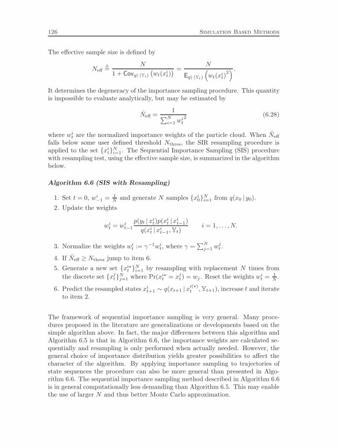
126 Simulation Based Methods
The effective sample size is defined by
NeffM=
N
1 + Covq(·|Yt)(wt(xit)
) =N
Eq(·|Yt)
(wt(xit)
2) .
It determines the degeneracy of the importance sampling procedure. This quantityis impossible to evaluate analytically, but may be estimated by
Neff =1∑N
i=1 wit2 (6.28)
where wit are the normalized importance weights of the particle cloud. When Neff
falls below some user defined threshold Nthres, the SIR resampling procedure isapplied to the set xitNi=1. The Sequential Importance Sampling (SIS) procedurewith resampling test, using the effective sample size, is summarized in the algorithmbelow.
Algorithm 6.6 (SIS with Resampling)
1. Set t = 0, wi−1 = 1N and generate N samples xi0Ni=1 from q(x0 | y0).
2. Update the weights
wit = wit−1
p(yt |xit)p(xit |xit−1)q(xit |xit−1,Yt)
i = 1, . . . , N.
3. Normalize the weights wit := γ−1wit, where γ =∑N
j=1 wjt .
4. If Neff ≥ Nthres jump to item 6.
5. Generate a new set xi?t Ni=1 by resampling with replacement N times fromthe discrete set xjtNj=1 where Pr(xi?t = xjt ) = wj . Reset the weights wit = 1
N .
6. Predict the resampled states xit+1 ∼ q(xt+1 |xi(?)t ,Yt+1), increase t and iterateto item 2.
The framework of sequential importance sampling is very general. Many proce-dures proposed in the literature are generalizations or developments based on thesimple algorithm above. In fact, the major differences between this algorithm andAlgorithm 6.5 is that in Algorithm 6.6, the importance weights are calculated se-quentially and resampling is only performed when actually needed. However, thegeneral choice of importance distribution yields greater possibilities to affect thecharacter of the algorithm. By applying importance sampling to trajectories ofstate sequences the procedure can also be more general than presented in Algo-rithm 6.6. The sequential importance sampling method described in Algorithm 6.6is in general computationally less demanding than Algorithm 6.5. This may enablethe use of larger N and thus better Monte Carlo approximation.

6.4 Recursive Monte Carlo Methods 127
Other recursive Monte Carlo approaches
The recursive SIR and the sequential importance sampling filters are the by farmost common particle filters for recursive estimation. A few alternative MonteCarlo approaches are summarized below.
Bølviken et al. [30] argue in favor of the rejection sampling method over theimportance sampling techniques described above. Their main argument is thatwith rejection sampling, a draw exactly from the posterior density is obtained,and no weighting of the candidate set is needed. But with the rejection samplingprocedure it is impossible to predict the number of iterations of the algorithm forobtaining a sample of fixed size N . Hence, it is not advisable to use rejectionsampling in on-line implementations.
Tanizaki [143] propose a non-recursive Monte Carlo filter and compares it with anumerical integration method and an importance sampling algorithm. The evalua-tion is performed using low dimensional linear and non-linear state space estimationbenchmark problems. The conclusion drawn by Tanizaki is that the proposed pro-cedure does not work well when the range of the state variables is unrestricted.Since the method is non-recursive it is not interesting for on-line applications.
The branching and interacting particle filters of Crisan et al. [41], and Del Moral[49] are similar to the algorithms presented in this subsection. The interactingparticle filters have a random number of particles that represent the posterior ateach iteration. The interacting particle filters coincide with the Bayesian bootstrapand the sequential importance sampling methods from a practical viewpoint, butare more restricted in the choice of proposal distribution. Greater emphasis isinstead put on theoretical considerations within this framework. Both Crisan et al.[41], and Del Moral [49] present several convergence results and they utilize arather general measure theoretic presentation. The framework is also applied tocontinuous time filtering. Some aspects on regularization of the particle methodsfor continuous time filtering are given by Le Gland et al. [108]. The regularizationis introduced to overcome problems with divergence of the particle cloud in priorimportance sampling.
6.4.2 Implementational Issues
Resampling
Resampling is required every iteration of the Bayesian Bootstrap filter, and when-ever Neff < Nthres in the sequential importance sampling procedure. A directimplementation of this resampling would consist of generating N i.i.d. variablesfrom U(0, 1), sort these in ascending order and compare them with the cumulativesum of the normalized weights. The best sorting algorithms has a complexity ofO(N logN), and it has been noted in practical applications that this severely limitsthe range of how far N can be increased.
Several approaches to suppress the complexity of the resampling step has beensuggested. Beadle and Djuric [10] decreases the computational burden by samplingevery candidate with equal probability but inserting several copies of the resampled
128 Simulation Based Methods
candidate each time it is chosen. The number of copies is proportional to theweight of the chosen candidate. The authors do issue a warning that samples withvery small weight will never be resampled at all using their method. However, asnoted by Doucet [60], the following classical algorithm for sampling N ordered i.i.d.variables uiNi=1 from U(0, 1) can be used to implement exactly the resampling inO(N) time.
Algorithm 6.7 (Sampling of ordered U(0, 1) variables [126, p. 96])
1. Sample ui ∼ U(0, 1), for i = 1, . . . , N .
2. Set uN = N√uN .
3. Compute ui = ui+1i√ui, for i = N − 1, . . . , 1.
In Matlab syntax this algorithm simply becomes
>> u = fliplr(cumprod(rand(1,N).^(1./(N:-1:1))));
which obviously is an O(N)-calculation. With an ordered i.i.d. sample from U(0, 1)at hand, the resampling is straightforwardly implemented by comparing this samplewith the cumulative sum of the normalized weights.
Optimal Importance Function
The choice of importance distribution will generally determine the performance ofthe algorithm and particularly the speed of degeneracy of the normalized weights.One way to choose a suitable q(xt |xt−1,Yt) is to select the function that minimizesthe degeneracy introduced in each iteration of the algorithm. The importancesampling distribution should thus minimize the variance of the importance weightswitNi=1, given the set of candidates at the previous step of the algorithm xit−1Ni=1,and the measurements Yt. Doucet [60] shows that the optimal choice for thiscriterion is given by
q(xt |xit−1,Yt) = p(xt |xit−1, yt).
With this choice of optimal importance function the importance weight recursionbecomes
wit ∝ wit−1
p(yt |xit)p(xit |xit−1)p(xit |xit−1, yt)
= wit−1 p(yt |xit−1).
In order to use the optimal importance function, one has to be able to sample fromp(xt |xit−1, yt) and to evaluate
p(yt |xit−1) =∫p(yt |xt)p(xt |xit−1) dxt,

6.4 Recursive Monte Carlo Methods 129
at least up to a normalization constant. In the general case this is impossible, butfor problems that can be written on the form
xt+1 = ft(xt) + wt
yt = Htxt + et(6.29)
with Gaussian independent noises, the optimal importance function is straightfor-wardly derived, see [60]. Doucet [60] suggests to utilize local linearization tech-niques when the problem is not on the form (6.29). We conclude the discussion onoptimal importance functions with an example of such techniques.
Example 6.3Consider the bearings-only tracking problem from Example 3.2. The state spacemodel for this recursive estimation problem is
x(1)t+1 = x
(1)t + w
(1)t
x(2)t+1 = x
(2)t + w
(2)t
yt = tan−1(x
(2)t /x
(1)t
)+ et.
This model is linear in the state update and nonlinear in the measurement rela-tion. A change to polar coordinates gives a nonlinear state update and a linearmeasurement relation
rt+1 =√r2t + w
(1)t rt sinϕt + w
(2)t rt cosϕt + w
(1)t w
(2)t
ϕt+1 = tan−1
(rt sinϕt + w
(2)t
rt cosϕt + w(1)t
)yt = ϕt + et.
The range state rt does not enter the likelihood, so the optimal proposal distri-bution for rit is the state transition equation given the candidate rit−1 and ϕit−1.The optimal proposal for the bearings state does not have a simple form, but alinearization of the coordinate transformation around rit−1 and ϕit−1 yields that
λit = Cov(ϕt | rit−1, ϕ
it−1
)≈ 2002
((sin(2ϕit−1)
2
)2
+(
cosϕit−1
rit−1
)2),
where the covariance matrix of the process noise wt from Example 3.2 has beeninserted. This suggests an approximatively optimal importance density given bythe Gaussian distribution
ϕt | rit−1, ϕit−1, yt ∼ N
(0.1ϕit−1 + λityt
0.1 + λit,
0.1λit0.1 + λit
)where the measurement noise covariance from Example 3.2 has been used. The ap-proximatively optimal importance distribution above can also be used to computeimportance weights.

130 Simulation Based Methods
Parallelizing the calculations
The weight update and particle diffusion can straightforwardly be calculated inde-pendently for each candidate state vector in the set. The resampling is howevernot possible to parallelize and this is also the part that is most time-consuming.Therefore it is of most importance that a good proposal is chosen to minimize thefrequency of resampling.
One way to achieve a parallel implementation is to run several particle filtersin parallel. A very high degree of parallelism cannot be achieved since each filterstill must have a rather large sample size N , so that the particle cloud of each filterresembles the posterior and does not diverge. The state estimates are based on aMonte Carlo average over the total set of all points in all filters, with the weightsappropriately normalized so that all the weights sum to unity.
6.4.3 Applications
The particle filters above have lately been applied to several recursive estimationproblems. Target tracking applications are very common to benchmark new ideasfor recursive estimation. Avitzour [5], Gordon [76], and the original article ofGordon et al. [78], use different versions of the recursive SIR. Other Monte Carloalgorithms for sequential target tracking in clutter is covered by Liu et al. [111],while target tracking in glint noise is considered by Gordon and Whitby [77].
In Chapter 7 the sequential algorithms above are applied to the terrain nav-igation application. Nonlinear recursive estimation problems arise frequently innavigation applications. Integration of inertial navigation system information withposition fixes from satellite systems such as GPS have been studied extensivelyand mainly tackled with extended Kalman filter techniques. Recently, Carvalhoet al. [39] presented simulation results using particle filters. Their conclusion is thatthe particle filters are greatly superior to the standard linearization techniques ofextended Kalman filtering.
6.5 Summary
The simulation based methods are general numerical integration and optimizationtools that are tightly coupled to the type of problems often occuring in Bayesianestimation. Integral estimation is performed by sample averaging over a largenumber of random samples generated from a desired distribution. The methods ofimportance and rejection sampling are suitable when an approximate description ofthe desired density is available. The suite of Markov Chain Monte Carlo methodsoffer solutions to problems of higher dimension, when it is harder to approximatelydescribe the density of interest.
For recursive estimation, the numerical integration methods of Chapter 5 andthe particle filters of this chapter are in several aspects very similar. Both representthe posterior density by a set of weighted points in the state space, and bothupdate this representation with respect to the incoming measurements. The main

6.5 Summary 131
difference though, is that for the numerical integration methods the grid is chosenby the user, while in the Monte Carlo methods it is more or less automaticallychosen by the model of the problem. The computational complexity of the standardnumerical integration methods grows exponentially with the size of the problem,while the particle filters in general do not suffer from such a limitation. Moreover,the particle filters are very simple to implement compared to the numerical, gridbased, methods.

132 Simulation Based Methods

7
Terrain Navigation
The terrain navigation application requires an on-line solution of a highly nonlinearrecursive estimation problem. In this work, we emphasize the statistical approachto recursive estimation in general, and the Bayesian paradigm in particular. Thebasic concept of terrain navigation is depicted in Figure 7.1. Measurements of ab-solute altitude, ground clearance, along with heading and speed information fromthe inertial navigation system are compared to a terrain reference map with theobjective of autonomously generating reliable position estimates of the aircraft inreal time. Chapter 2 presented a background to the terrain navigation application,the stochastic modeling of the problem, the optimal but intractable Bayesian solu-tion, and an approximative implementation. The point-mass implementation wasfurther detailed in Chapter 5. A simulation study presented in Chapter 2, showedthat the suboptimal Bayesian point-mass filter (PMF) yields high navigation per-formance in realistic simulations. The recursive estimation model for the terrainnavigation problem was given in (2.4),
xt+1 = xt + ut + wt
yt = h(xt) + ett = 0, 1, . . . (7.1)
accompanied by density functions for the initial position x0, and the disturbanceset and wt, respectively. It is the unstructured nonlinear terrain map, entering themeasurement equation of the model (7.1), that makes this problem challenging.
133

134 Terrain Navigation
Altitude Ground clearance
Mean sea-level
Terrain elevation
Figure 7.1: The principle of terrain navigation.
The general overview of the terrain navigation application given in Chapter 2 iscomplemented by some additional background material in Section 7.1. The sectioncontains a discussion regarding the concept of integrating the position estimatesfrom the terrain navigation system with the inertial navigation system. A detaileddescription of previously presented approaches to this application is also given inSection 7.1. A much more detailed description of the terrain navigation applicationcan be found in Bergman [16]. Characteristics of the sensors, and discussionsregarding methods for estimating the vertical bias error are some of the topicshandled in [16]. In Section 7.2, we utilize both the parametric and the posteriorCramer-Rao bounds from Chapter 4 in a Monte Carlo evaluation of the PMFimplementation. The posterior Cramer-Rao bound is also linked to the informationcontent in the terrain map in Section 7.3. Section 7.4 presents three particle filtersfrom Chapter 6 applied to terrain navigation. These filters are evaluated againstthe Cramer-Rao bounds and the PMF implementation.
7.1 Application Background
The main advantage with the principle of terrain navigation, depicted in Figure 7.1,is that it yields position estimates autonomously. This navigation principle doesnot have to rely on support of any satellite or terrestrial radio system broadcast-ing information to the aircraft. However, terrain navigation will not work overthe sea, over big lakes, over very flat terrain or while flying at large ground clear-

7.1 Application Background 135
ance distances. It does, on the other hand, perform equally well under electroniccountermeasure conditions, during day or night, and in all possible weather condi-tions [135]. There are several ways to utilize the components of a terrain navigationsystem for other tasks than sole support for an inertial navigation system. Sug-gestions of using terrain navigation for ground obstacle collision avoidance, terrainfollowing and mission planning are given in [86, 87].
7.1.1 Integration of Navigation Systems
In the aircraft navigation application, ensuring the safety of the passengers is acritical issue. Errors in the construction of the navigation system or physical mal-functions of sensors may cause severe damage with risk for human life. Modernaircraft navigation systems therefore consist of several separate or partly separatenavigation devices, where each device produces estimates of a subset of the needednavigation parameters. The output from the individual devices are combined,usually by means of a Kalman filter, to generate the complete set of navigation pa-rameters of the aircraft. The redundancy between the devices can also be utilizedto detect and isolate malfunctions in the different systems and thereby increasethe overall system integrity. A comprehensive treatment of integrity monitoring ofnavigation systems is given by Palmqvist [119].
Inertial navigation systems can track highly dynamical motion very well overlimited time intervals. However, the open loop configuration of inertial systemsyields an inevitable, slowly varying, and growing error in the system output. Aterrain navigation system supporting the inertial system with frequent positionupdates will limit this long term divergence while retaining the autonomous featureof the navigation application. On the other hand, the terrain navigation systemdemands heading and velocity information for maximum performance. Thus, asymbiosis constellation between an inertial navigation and a terrain navigationsystem will yield an integrated system with high performance on both a long anda short time scale.
The inertial system determines the aircraft position by integrating measure-ments of the aircraft acceleration in real time. The integration result is trans-formed into a fixed coordinate system using measurements of the aircraft angularrates. Let a(t) denote a vector of measured acceleration and angular rates, and x(t)denote the state vector of the inertial navigation system (INS). The state vectortypically consists of the aircraft position, velocity and attitude together with thegyro and accelerometer states. The dynamic integration performed by the INS isdescribed by a nonlinear differential equation,
x(t) = ft(x(t)
)+ gt
(a(t)
). (7.2)
where the nonlinear functions ft(·) and gt(·) involve different coordinate transfor-mations [99]. If the acceleration and gyro measurements were noiseless, the INSstate would be in perfect resemblance with the true state of the aircraft, denotedby x0(t). Likewise, letting a0(t) denote the actual acceleration and angular rates

136 Terrain Navigation
of the aircraft the true state evolves according to a similar differential equation
x0(t) = ft(x0(t)
)+ gt
(a0(t)
). (7.3)
Denote the aircraft position estimates produced by the terrain navigation systemby y(t). Neglecting that these are driven by the velocity estimates from the INS,the relation between the aircraft state vector and the position “measurement” fromthe terrain navigation algorithm can be described as
y(t) = ht(x0(t)
)+ e(t). (7.4)
Above, the nonlinear function ht(·) is the coordinate transformation of the positionelements in x0(t) to the navigation frame of the terrain navigation filter. Themeasurement noise, e(t), in (7.4) is the estimation error in the position estimate ofthe terrain navigation filter.
Let xδ(t) and aδ(t) be the errors in the INS state vector and the accelerationmeasurements, i.e.,
x0(t) = x(t) + xδ(t)a0(t) = a(t) + aδ(t).
(7.5)
Assuming that these errors are small, we neglect the second and higher order termsin a Taylor expansion of (7.3) and (7.4) around x(t) and a(t). Using (7.2) and (7.5)yields that the error state satisfies a linearized dynamical model
xδ(t) =∂ft(x)∂x
∣∣∣x=x(t)
xδ(t) +∂gt(a)∂a
∣∣∣a=a(t)
aδ(t)
y(t)− ht(x(t)
)=∂ht(x)∂x
∣∣∣x=x(t)
xδ(t) + e(t).(7.6)
This model describes the errors dynamics in the inertial navigation system, andhow the terrain navigation estimate can be used as a measurement of these errors.Modeling the acceleration error aδ(t) by a fixed Gaussian distributed vector over asmall time interval, the system (7.6) is discretized and can be used to implementan extended Kalman filter estimator for xδ(t). Figure 7.2 shows a schematic blockdiagram of the integration of terrain navigation and inertial navigation, and thesystem output is labeled x0(t). Since the terrain navigation filter is driven by thevelocity estimate of the INS, the estimated error in this velocity is fed back fromthe Kalman estimator to the terrain navigation filter. In Figure 7.2, the notationvδ(t) has been adopted for the estimated error in the velocity used in the terrainnavigation algorithm, and the abbreviation TNF stands for terrain navigation filter.Note that in the linearization scheme in the extended Kalman filter, the systemmatrices should be evaluated at x(t) and a(t) and thus the Kalman filter actuallydepends on the INS state vector. This has not been depicted in Figure 7.2.
The integration, using terrain information to estimate the INS errors, demandsa quantization of the estimation error covariance, utilized as measurement errorcovariance in the Kalman filter. Since this estimation error will depend on the
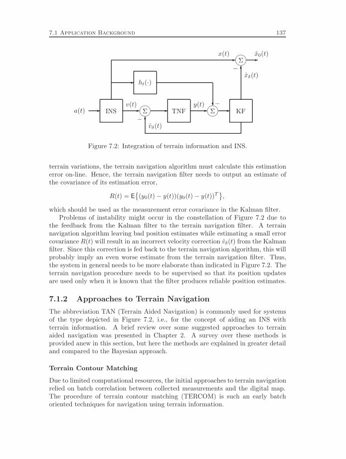
7.1 Application Background 137
-a(t) INS -v(t) Σ - TNF -
y(t) Σ6vδ(t)
- KF
6xδ(t)
Σ -x0(t)
-x(t)
- ht(·)
?
−
−
−
Figure 7.2: Integration of terrain information and INS.
terrain variations, the terrain navigation algorithm must calculate this estimationerror on-line. Hence, the terrain navigation filter needs to output an estimate ofthe covariance of its estimation error,
R(t) = E
(y0(t)− y(t))(y0(t)− y(t))T,
which should be used as the measurement error covariance in the Kalman filter.Problems of instability might occur in the constellation of Figure 7.2 due to
the feedback from the Kalman filter to the terrain navigation filter. A terrainnavigation algorithm leaving bad position estimates while estimating a small errorcovariance R(t) will result in an incorrect velocity correction vδ(t) from the Kalmanfilter. Since this correction is fed back to the terrain navigation algorithm, this willprobably imply an even worse estimate from the terrain navigation filter. Thus,the system in general needs to be more elaborate than indicated in Figure 7.2. Theterrain navigation procedure needs to be supervised so that its position updatesare used only when it is known that the filter produces reliable position estimates.
7.1.2 Approaches to Terrain Navigation
The abbreviation TAN (Terrain Aided Navigation) is commonly used for systemsof the type depicted in Figure 7.2, i.e., for the concept of aiding an INS withterrain information. A brief review over some suggested approaches to terrainaided navigation was presented in Chapter 2. A survey over these methods isprovided anew in this section, but here the methods are explained in greater detailand compared to the Bayesian approach.
Terrain Contour Matching
Due to limited computational resources, the initial approaches to terrain navigationrelied on batch correlation between collected measurements and the digital map.The procedure of terrain contour matching (TERCOM) is such an early batchoriented techniques for navigation using terrain information.

138 Terrain Navigation
Prior to the flight mission, several areas with high terrain variations are iden-tified along the aircraft flight path. Reference matrices of the terrain elevation inthese areas are stored in the system computer. These matrices are interpolatedand aligned according to the planned vehicle orientation so that the correlationcan be performed easily along the columns of the corresponding reference matrixH . Hence, the system demands that the vehicle does not manoeuvre during thedata gathering, and that it has approximately correct orientation. During flight,the radar altimeter is tuned to sample the terrain elevation with a sample periodadjusted so that the collected terrain elevation profile will have the same distancebetween consecutive samples as the distance between samples in the reference ma-trix H .
The most common way to perform the correlation in the TERCOM systemsis to find the position in the reference matrix that minimizes the mean absolutedifference (MAD) between the terrain elevation profile and the reference matrix.The MAD value is computed by calculating the absolute value of the errors alongthe profile and taking the mean of these absolute errors. Gathering N samples,the algorithm computes the MAD for the profile of every column m and every rowdisplacement k in the matrix H ,
MADk,m =1N
N∑n=1
|yn −Hm,n+k|.
The algorithm chooses the position with best correlation
(k, m) = arg mink,m
MADk,m.
Even if the technique is old and puts severe restrictions on the manoeuvres of theaircraft, the basic TERCOM-approach is still used in several applications today.The TERCOM system is mainly used for unmanned and rarely manoeuvring vehi-cles such as cruise-missiles, detailed descriptions of this algorithm are provided byBaker and Clem [6], Golden [75], Siouris [135].
Sandia Inertial Terrain Aided Navigation
Sandia Inertial Terrain Aided Navigation (SITAN) is the label on a terrain navi-gation scheme developed at Sandia Laboratories in the late 1970s. SITAN is theearliest reported approach of a recursive solution to the terrain matching problem.The algorithm uses a modified version of an extended Kalman filter (EKF) in itsoriginal formulation by Hostetler [91]. In order to diminish the effect of terrainnonlinearities, a certain adaptive stochastic linearization technique is used in thealgorithm of [91].
Several modifications of the original SITAN approach have been proposed. Inorder to overcome divergence problems in the filter estimates parallel EKFs havebeen used by Hollowell [88], and Boozer and Fellerhoff [31]. The rationale behindthese extensions is that while linearizing the filters in different positions over an
7.1 Application Background 139
area where the aircraft is supposed to be, the sensitivity to the nonlinear terrain islimited. In [31] each Kalman filter has three error states; the navigation system’seasting, northing and vertical error. The idea is that as the measurements areprocessed, some filters will cluster around the true position and an estimate of thenavigation errors can be formed. In the highly manoeuvring helicopter applicationconsidered by Hollowell [88], the filters are scalar and it is only the vertical bias thatis estimated. Here, the grid of filters is fixed but translated with the movement ofthe helicopter, and an estimate of the position is formed by averaging over estimatesfrom certain filters with small estimation error.
Terrain Profile Matching
The British Aerospace system Terrain Profile Matching (TERPROM) is commonlyused in several military aircraft. A rather brief, and not very detailed, description ofthe TERPROM system is given by Davies [44]. The algorithm is a hybrid solutionwhich in acquisition-mode correlates measurements in batch to find an initial posi-tion, and in track-mode processes measurements recursively using Kalman filteringtechniques.
Viterbi Algorithm Terrain Aided Navigation
Enns and Morrell [64] propose to use a discretized version of the continuous Viterbialgorithm in the terrain navigation application. Their Viterbi Algorithm TerrainAided Navigation (VATAN) algorithm computes approximatively a maximum aposteriori estimate of the aircraft horizontal position. The implementation usesa grid over the area of interest and translates this grid along with measurementsfrom the inertial navigation system. The metric Lt(xt) is initiated by the priordescription of the aircraft position, L0(x0) = log p(x0), and calculated for eachgrid point according to the recursion
Lt+1(xt+1) = log p(yt+1 |xt+1) + maxxtlog p(xt+1 |xt) + Lt(xt) .
The position maximizing this metric is used as an estimate of the aircraft position
xt = arg maxxt
Lt(xt).
The algorithm has not been reported used in any field tests, but in simulationsdescribed in [64] it outperforms the single EKF version of the SITAN algorithm.
Bayesian Terrain Navigation
The Bayesian solution to terrain navigation was presented in Chapter 2. Theidea behind this approach is to model the recursive nonlinear inference problemin terrain navigation as accurately as possible in a statistical framework, and tocompute a good approximation to the optimal Bayesian solution of this model.The main difference between this approach and the ones described previously is

140 Terrain Navigation
that no linearization of the nonlinear terrain elevation map is needed. Instead, anapproximate description of the unstructured posterior density is recursively propa-gated by the numerical integration method of Algorithm 5.1, the point mass filter(PMF). The PMF computes a discretized approximation to the probability densityfunction of the aircraft position and recursively updates this discrete density witheach new measurement from the radar altimeter and with the aircraft movementestimate from the inertial navigation system. The grid mesh resolution and supportis controlled through three design parameters.
The main advantages of this approach were reviewed in Chapter 2. The mostimportant issue for the terrain navigation application is the ability of the PMF totrack several position hypotheses in parallel. An illustration of this ability is givenin Figure 7.3 which depicts six consecutive point-mass approximations from therealistic simulations presented in Chapter 2. The point-mass approximations are
Iteration tIteration t+ 1
Iteration t+ 2 Iteration t+ 3
Iteration t+ 4Iteration t+ 5
Figure 7.3: The point-mass approximation of the posterior will have several peaksif the terrain is repetitive.
extracted from a section of the simulations performed over the track in Figure 2.5having informative, but repetitive, terrain characteristics. At iteration t the condi-tional density approximation has a unique maximum but a rather wide support oflow, but not negligible, point mass values. Due to the underlying terrain charac-

7.2 Cramer-Rao Bound Evaluation 141
teristic, the density splits up into two equally high peaks during the following twoiterations. When the aircraft reaches an area of less repetitive terrain, a few moremeasurements are processed and the false peak is effectively attenuated.
The effects depicted in Figure 7.3, and the realistic simulation study describedin Chapter 2 justify that the PMF solution is well suited for the terrain navigationapplication. The PMF has also been verified against real flight test data, reportedin the Master Thesis work of Svensson [140]. According to Svensson [140], thePMF yields equally good navigation performance in the realistic simulations ason real data. It is mainly the possibility to utilize a detailed model of the noisedistributions p(et) and p(wt), and the ability of the point-mass density to accuratelydescribe the position information, that yield the encouraging results of the PMF.Still, in a practical application it is not fully understood how to model the noisedistributions p(et) and p(wt), and how to maximize the utility of the point-massdensity. In [140], the PMF is working in conjunction with a Kalman filter forestimating the vertical position error. This constellation is suggested in [16], andbased on the principle of certainty equivalence.
In the following section we evaluate the average performance of the PMF usingMonte Carlo simulations of the terrain navigation application. Less emphasis hashere been put on the realism of the simulation conditions, and the resulting navi-gation error therefore only plays a minor role. Instead, we use noise distributionsfor which the Cramer-Rao bound for the estimation problem is easily determinedand the Monte Carlo performance is compared to this fundamental bound.
7.2 Cramer-Rao Bound Evaluation
The PMF computes an approximative description of the posterior density. In thissection we apply the fundamental Cramer-Rao bounds from Chapter 4 to verify thatthe effect of this approximation does not seriously alter the algorithm performance.We utilize Monte Carlo simulations to determine the average performance of thealgorithm in two different areas, having smooth and rough terrain, respectively.
Even if the PMF is derived in a Bayesian framework, it can be evaluated in aparametric or Bayesian Monte Carlo setting. In the parametric setting, the statetrajectory is fixed x?i Ni=1, and independent measurement noise is generated in Midentical Monte Carlo runs. The navigation filter is applied to these data, resultingin the estimated tracks xitMi=1. Considering the one step ahead prediction ofthe aircraft position, the Monte Carlo approximation to the Cramer-Rao boundinequality was provided in Section 4.5 as√√√√ 1
M
M∑i=1
‖xit − x?t ‖2 &
√trPt t = 1, . . . , N (7.7)
where Pt is given by Theorem 4.3. We use a Gaussian distributed initial positionwith covariance P0, and Gaussian noises wt and et, with covariance Q and R,respectively. The parametric Cramer-Rao bound then follows by inserting the

142 Terrain Navigation
model (7.1) and these noise distributions into Theorem 4.3,
Pt+1 = Pt − PtHt(HTt PtHt +R)−1HT
t Pt + Q where Ht = ∇xh(x)x=x?t
is the gradient of the terrain evaluated at the true aircraft positions along the fixedtrack.
In the Bayesian Monte Carlo evaluation, M independent tracks are generatedfrom (7.1) yielding M random walk realizations in two dimensions. The filteris applied to each of these tracks using measurements of the ground clearancecorrupted by independently distributed measurement noise. The resulting one stepahead position estimate at time t in Monte Carlo run i is denoted xit. Section 4.5yields the Cramer-Rao bound inequality√√√√ 1
M
M∑i=1
‖xit − xit‖2 &
√trPt t = 1, . . . , N (7.8)
where Pt is given by Theorem 4.5. With the Gaussian noise assumption insertedinto the model (7.1) we have that
P−1t+1 = Q−1 −Q−1(P−1
t + Zt +Q−1)−1Q−1 (7.9a)
where
Zt = R−1 E(∇xth(xt)(∇xth(xt))T
)(7.9b)
since R is scalar and constant. The Monte Carlo estimate of this quantity is givenby the sample average over the M independent tracks. The posterior bound isthus computed by averaging the terrain gradient over all the M tracks, while theparametric bound is computed from the terrain gradient at the positions given ina single track.
The minimum mean-square error, or minimum variance, estimate is the con-ditional mean of the posterior density. In the PMF approximation, it is given bythe center of gravity of the point mass approximation. If the posterior density wasperfectly described by the PMF, the minimum variance estimate would by con-struction satisfy the Cramer-Rao bound inequalities (7.7) and (7.8). The observeddiscrepancy from the Cramer-Rao bound in the Monte Carlo evaluation below cantherefore be traced to the approximative point-mass density.
Table 7.1 summarizes the actual noise levels, track duration and Monte Carloiterations used in the simulations. Two different parts of the terrain map were usedin these simulations. These terrain areas are shown in Figure 7.4. The figure alsodepicts 200 of the tracks used in both the smooth and rough posterior Cramer-Raobound evaluations. One of these tracks was extracted for the respective parametricCramer-Rao bound evaluation, this track is highlighted in Figure 7.4. The PMFperformance naturally depends on the parameters that affect the grid resolutionand update. The chosen settings are summarized in Table 7.2. The grid truncation

7.2 Cramer-Rao Bound Evaluation 143
0
1000
2000
3000
4000
5000
6000
0
1000
2000
3000
4000
5000
6000
100
150
200
0
1000
2000
3000
4000
5000
6000
0
1000
2000
3000
4000
5000
6000
0
50
100
Figure 7.4: The rough and smooth simulation areas, the axes are labeled in meterscale. The first 200 simulation tracks used in the posterior simulations are shownover each map, the track used for the parametric evaluation is highlighted in white.

144 Terrain Navigation
Initial covariance P0 = 2002I2 m2
State noise covariance Q = 52I2 m2
Measurement noise covariance R = 4 m2
Track length 300 samplesMonte Carlo runs 1000
Table 7.1: The simulation settings.
Initial grid resolution δ = 50 mResampling limits N0 = 1000
N1 = 5000Truncation parameter ε = 0.001
Table 7.2: Filter parameters.
and resampling parameters are identical to the ones used in the realistic simulationevaluation presented in Chapter 2.
The simulation results in the parametric Monte Carlo evaluations are depictedin Figure 7.5. Initially, a sparse grid with 50 m space between each grid point is
0 50 100 150 200 250 3000
50
100
150
200
250
300
met
er
time0 50 100 150 200 250 300
0
50
100
150
200
250
300
met
er
time
Figure 7.5: Monte Carlo root mean square error (solid) compared to the parametricCramer-Rao bound (dashed) for the rough (left) and smooth (right) simulationareas.
used in the point-mass approximation. The grid resolution is successively increasedby the PMF grid update when more information becomes available, and, afterconvergence, the grid resolution keeps oscillating between 6.25 m and 3.125 m. Overthe rough terrain area, each measurement yields valuable information about theaircraft position and the PMF rapidly converges to a stationary error level. After

7.2 Cramer-Rao Bound Evaluation 145
the convergence, remains in the vicinity of the bound for the remaining simulationtime. Over the smooth terrain area, the less informative measurements yield a lessrapid increase of the grid resolution. The sparse initial mesh, with 50 m betweeneach grid point, clearly yields suboptimal performance during the first third ofthe simulation track. However, when the grid resolution increases, the algorithmperformance reaches the bound and stays close to it for the remaining simulationtime. During both the rough and the smooth case, the error occasionally reachesbelow the bound. This effect may origin from a bias towards the fixed unknownaircraft track. The effect does not seem to disappear by increasing the number ofMonte Carlo iterations.
Applying the PMF to 1000 different aircraft trajectories, the Monte Carlo RMSerror and corresponding posterior Cramer-Rao bound are shown in Figure 7.6.Since both the bound and the Monte Carlo RMS error are averaged over the ter-
0 50 100 150 200 250 3000
50
100
150
200
250
300
met
er
time0 50 100 150 200 250 300
0
50
100
150
200
250
300
met
er
time
Figure 7.6: Monte Carlo root mean square error (solid) compared to the posteriorCramer-Rao bound (dashed) for the rough (left) and smooth (right) simulationareas.
rain area in this case, the plots show a smoother behavior than the parametriccounterpart. In all other aspects, the results shown in Figure 7.6 indicate a similarpattern to the parametric case. The rough terrain case gives a fast convergenceand close to optimal mean square error, while the smooth terrain area yields aslower convergence but equally good steady state performance. The error does notreach below the posterior bound in either the rough or the smooth case. Since theposterior Cramer-Rao bound does not assume an unbiased estimator, this indicatesthat the explanation of the super-effectiveness in the parametric case is sound.
The Cramer-Rao bound has been applied to the evaluation of a point-massapproximation to the Bayesian approach to terrain navigation. In several exhaus-tive Monte Carlo simulations over different types of terrain, the point-mass filteris shown to meet the bound as the approximation grid becomes dense. The filterperformance is suboptimal during the settling phase, but after the initial conver-gence, the filter yields near optimal performance. In the parametric evaluation, it
146 Terrain Navigation
occasionally happens that the mean square estimation error falls slightly below theCramer-Rao bound. This probably origins from a bias-variance tradeoff since suchbehavior is not observed in the posterior case.
The Monte Carlo simulations presented above reveal the average performanceof the approximate Bayesian inference procedure given in Algorithm 5.1. The factthat the mean square error of the PMF reaches the Cramer-Rao bound when thegrid resolution becomes sufficiently dense, shows that the point-mass descriptionsucceeds in approximating the conditional filter density.
7.3 Terrain Information
The absolute performance of any terrain navigation filter will inevitably dependon the amount of information about the aircraft position revealed by the terrainelevation measurements. This fact is clearly obvious in the simulation results ofthe previous section. In this section, we connect the posterior Cramer-Rao boundto the scalar terrain information measure (2.1), suggested in Chapter 2.
Let S be an arbitrary region of size A inside the terrain elevation map. Considerthe Bayesian estimation problem with an initial position, uniformly distributed overthe region S,
p(x) =
A−1 for x ∈ S
0 elsewhere.
and a single measurement from the relation
y = h(x) + e
available. Let the additive scalar measurement noise be Gaussian distributed withzero mean and variance λ. The joint density of the states and the measurement is
p(x, y) = p(y |x) p(x) =
A−1 N(y;h(x), λ) for x ∈ S
0 elsewhere.
Taking the logarithm of this density yields
log p(x, y) =
− 1
2λ (y − h(x))2 + C for x ∈ S
−∞ elsewhere,
where C is a constant, not depending on x. Hence, the “information matrix” forthe Bayesian estimation problem outlined above becomes
J = E(−∆xx log p(x, y)) =
1λ
E(∇xh(x)∇Tx h(x)− (y − h(x))∆x
xh(x)).
Since the measurement noise e is assumed to have zero mean, we have that
J =1λ
E(∇xh(x)∇Tx h(x)
)=
1λA
∫S
∇xh(x)∇Tx h(x) dx,
7.4 Monte Carlo Filters 147
since the prior distribution of the states is uniform over the region S. With a MonteCarlo approximation of this expression, a scalar terrain information measure isgiven by the expression suggested in (2.1),
√tr J ≈
√√√√ 1N
N∑i=1
‖∇xih(xi)‖2,
where the points xi are uniformly distributed over the area of interest. This infor-mation measure coincides with the one proposed in (2.1).
7.4 Monte Carlo Filters
The simulation based algorithms for recursive estimation presented in Chapter 6utilize Monte Carlo integration techniques for approximative Bayesian estimation.Applied to terrain navigation, these filters will recursively generate a large numberof candidate positions of the aircraft and determine likelihood weights assignedto each candidate trajectory. In this section we present extensive Monte Carloevaluations using three different simulation based particle filters from Chapter 6.The Bayesian bootstrap, the sequential importance sampling and the linearizedoptimal importance sampling methods are studied. The simulation results arecompared to the Cramer-Rao bound and the point-mass filter of Algorithm 5.1from Section 5.2.
Assuming that the absolute altitude of the aircraft is known, or has been esti-mated with a small error, the objective of the terrain navigation procedure is todetermine the aircraft position projected on the terrain map. The two dimensionalmodel for this recursive estimation problem is,
xt+1 = xt + ut + vt
yt = h(xt) + ett = 0, 1 . . . (7.10)
For simplicity, the noises vt and et are chosen to be Gaussian distributed, yieldingthat the posterior Cramer-Rao bound for the estimation problem is given by (7.9).The noise distributions and parameters in this evaluation are not primarily chosento give realistic results for the navigation application. This is less important sincecomparisons are made relative to the Cramer-Rao bound. Here, we are primarilyinterested in the average relative performance of the different algorithms studied.The chosen parameters are summarized in Table 7.3. Gaussian distributed initialpositions of the Monte Carlo tracks were generated with a fixed average positionx0, and covariance P0 given in Table 7.3. The resulting tracks generated fromindependent realizations of the system and measurement noises are depicted inFigure 7.7. The terrain map is shown as a contour plot behind the tracks. Thisis a part of the same commercial map used in the previously presented terrainnavigation simulations. The posterior Cramer-Rao bound (7.9) was computed usingthese simulated tracks over the map.

148 Terrain Navigation
Initial covariance P0 = 1002I2 m2
State noise covariance Q = 52I2 m2
Measurement noise covariance λ = 16 m2
Track length 150 samplesAircraft velocity ut = [25, 25]T m/sample
Monte Carlo runs 100
Table 7.3: Parameters for the simulated tracks.
Figure 7.7: The 100 simulated aircraft tracks are depicted over a contour map ofthe commercial terrain map. The simulated aircraft tracks start in the lower leftcorner and ends in the upper right corner of the map.
The Bayesian bootstrap filter, Algorithm 6.5, performs resampling after eachmeasurement update. Applying this algorithm to the terrain navigation model (7.10)with parameters given in Table 7.3 yields the procedure summarized below.
Algorithm 7.1 (Bayesian bootstrap)
1. Set t = 0, and generate N samples xi0Ni=1 from N(x0, P0).

7.4 Monte Carlo Filters 149
2. Compute the normalized weights
wi =N(yt;h(xit), λ)∑Nj=1 N(yt;h(xjt ), λ)
i = 1, . . . , N
and determine the estimate xt =∑Ni=1 wix
it.
3. Generate a new set xi?t Ni=1 by resampling with replacement N times fromthe discrete set xjtNj=1 where Pr(xi?t = xjt ) = wj .
4. Generate vit ∼ N(0, Q) for i = 1, . . . , N , and predict the particle cloud
xit+1 = xi?t + ut + vit i = 1, . . . , N.
5. Set t := t+ 1 and repeat at item 2.
In comparison to a Kalman filter algorithm, item 2 and 3 correspond to a mea-surement update step, while item 4 is the time update. Identical Monte Carlosimulations were performed over the tracks in Figure 7.7 using sample sizes Nranging from 50 to 800. Figure 7.8 shows the resulting Monte Carlo root meansquare error using Algorithm 7.1. The figure also shows the fundamental posteriorCramer-Rao bound for the set of simulation tracks. The Monte Carlo root meansquare error naturally decreases with increasing sample size N , although not mono-tonically. For the sample sizes 200 and higher, the average error after convergenceis almost equal, while the speed of convergence still increases for higher samplesizes. The reason for this effect is that the aircraft position is very uncertain andthe posterior filter density has a large support at the initialization of the algo-rithms. A large set of samples is better at approximating this posterior with widesupport during the settling phase, while the algorithms using fewer samples yielda less correct description of the filter density. In the extreme case, few sampleswill even lead to algorithm divergence due to an incorrect description of the filterdensity. After half sample number 100, the filter density has become rather nar-row and comparable result are obtained at almost all sample sizes. Algorithm 7.1converges to an average error very close to the Cramer-Rao bound for all samplesizes N > 50.
In the sequential importance sampling algorithm, Algorithm 6.6, the degeneracyof the weights determines when to perform resampling. The algorithm describedbelow, is the sequential importance sampling method with importance functiongiven by the approximative prior p(xt |Yt−1) from the last iteration.
Algorithm 7.2 (Importance Sampling)
1. Set t = 0, wi−1 = 1N and generate N samples xi0Ni=1 from N(x0, P0).

150 Terrain Navigation
0 50 100 1500
50
100
150
time
m
N=50 N=100 N=200 N=400 N=800 Cramer−Rao Bound
Figure 7.8: Monte Carlo RMS error and posterior Cramer-Rao bound for theBayesian bootstrap filter, Algorithm 7.1.
2. Update the weights
wit = wit−1 N(yt;h(xit), λ) i = 1, . . . , N
and normalize them
wit :=wit∑Nj=1 w
jt
i = 1, . . . , N.
Compute the estimate xt =∑N
j=1 witxit.
3. If Neff < Nthres resample with replacement from the set xitNi=1 where wit isthe probability of resampling the state xit. Reset the weights wit = 1
N .4. Generate vit ∼ N(0, Q) for i = 1, . . . , N , and predict the particle cloud
xit+1 = xit + ut + vit i = 1, . . . , N.
5. Set t := t+ 1 and repeat at item 2.
The effective sample size was defined in (6.28), as
Neff =1∑N
i=1 wit2
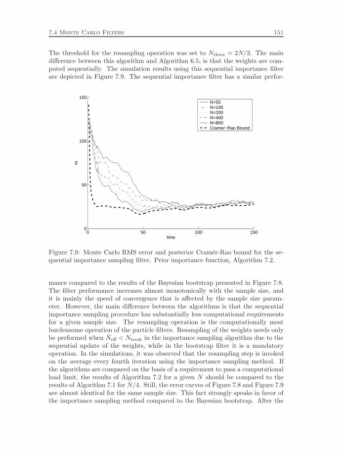
7.4 Monte Carlo Filters 151
The threshold for the resampling operation was set to Nthres = 2N/3. The maindifference between this algorithm and Algorithm 6.5, is that the weights are com-puted sequentially. The simulation results using this sequential importance filterare depicted in Figure 7.9. The sequential importance filter has a similar perfor-
0 50 100 1500
50
100
150
time
m
N=50 N=100 N=200 N=400 N=800 Cramer−Rao Bound
Figure 7.9: Monte Carlo RMS error and posterior Cramer-Rao bound for the se-quential importance sampling filter. Prior importance function, Algorithm 7.2.
mance compared to the results of the Bayesian bootstrap presented in Figure 7.8.The filter performance increases almost monotonically with the sample size, andit is mainly the speed of convergence that is affected by the sample size param-eter. However, the main difference between the algorithms is that the sequentialimportance sampling procedure has substantially less computational requirementsfor a given sample size. The resampling operation is the computationally mostburdensome operation of the particle filters. Resampling of the weights needs onlybe performed when Neff < Ntresh in the importance sampling algorithm due to thesequential update of the weights, while in the bootstrap filter it is a mandatoryoperation. In the simulations, it was observed that the resampling step is invokedon the average every fourth iteration using the importance sampling method. Ifthe algorithms are compared on the basis of a requirement to pass a computationalload limit, the results of Algorithm 7.2 for a given N should be compared to theresults of Algorithm 7.1 for N/4. Still, the error curves of Figure 7.8 and Figure 7.9are almost identical for the same sample size. This fact strongly speaks in favor ofthe importance sampling method compared to the Bayesian bootstrap. After the

152 Terrain Navigation
settling phase, the RMS error of Algorithm 7.2 converges to a level close to theCramer-Rao bound for all sample sizes studied.
The use of the posterior density as importance function can make the sequentialimportance sampling filter sensitive to outlier measurements. A better choice ofimportance function can also decrease the rate of the inevitable weight degeneracy.The optimal importance function, presented in Section 6.4.2, is chosen to minimizethe weight degeneracy at each algorithm recursion. For the terrain navigationproblem, given on the form (7.10), it is not possible to exactly sample from theoptimal distribution. In the local linearization techniques promoted by Doucet[60], each sample candidate is drawn from a distribution that is a local Gaussianapproximation to the true optimal distribution. In the particle prediction step, thecandidate xit is generated from a Gaussian distribution with covariance and meangiven by
Σit = Q−Qht,ihTt,iQ/(hTt,iQht,i + λ)
µit = Σit(Q−1(xit−1 + ut−1) + ht,i(yt − h(xit) + hTt,i(x
it−1 + ut−1))/λ)
(7.11)
where ht,i = ∇h(xit), λ and Q are noise covariances from Table 7.3. The derivationis straightforward and can be found in [60]. Note though, that this technique onlyworks with Gaussian noises et and vt. Hence, the linearized optimal importancefunction is not applicable in the true terrain navigation application without someadditional approximations since at least the measurement noise et is regarded asnon-Gaussian. The resulting importance filter using a locally Gaussian optimalimportance function follows.
Algorithm 7.3 (Optimal Importance Sampling)
1. Set t = 0, wi−1 = 1N and generate N samples xi0Ni=1 from N(x0, P0).
2. For each i = 1, . . . , N compute µit and Σit. Generate new samples
xit ∼ N(µit,Σit) i = 1, . . . , N
3. Update the weights
wit = wit−1
N(yt;h(xit), λ) N(xit;xit−1 + ut−1, Q)
N(xit;µit,Σit)i = 1, . . . , N
and normalize them
wit :=wit∑Nj=1 wj
i = 1, . . . , N.
Compute the estimate xt =∑N
j=1 witxit.
4. If Neff < Nthres resample with replacement from the set xitNi=1 where wit isthe probability of resampling the state xit. Reset the weights wit = 1
N .
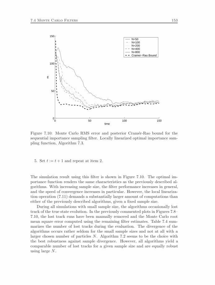
7.4 Monte Carlo Filters 153
0 50 100 1500
50
100
150
time
m
N=50 N=100 N=200 N=400 N=800 Cramer−Rao Bound
Figure 7.10: Monte Carlo RMS error and posterior Cramer-Rao bound for thesequential importance sampling filter. Locally linearized optimal importance sam-pling function, Algorithm 7.3.
5. Set t := t+ 1 and repeat at item 2.
The simulation result using this filter is shown in Figure 7.10. The optimal im-portance function renders the same characteristics as the previously described al-gorithms. With increasing sample size, the filter performance increases in general,and the speed of convergence increases in particular. However, the local lineariza-tion operation (7.11) demands a substantially larger amount of computations thaneither of the previously described algorithms, given a fixed sample size.
During all simulations with small sample size, the algorithms occasionally losttrack of the true state evolution. In the previously commented plots in Figures 7.8–7.10, the lost track runs have been manually removed and the Monte Carlo rootmean square error computed using the remaining filter estimates. Table 7.4 sum-marizes the number of lost tracks during the evaluation. The divergence of thealgorithms occurs rather seldom for the small sample sizes and not at all with alarger chosen number of particles N . Algorithm 7.2 seems to be the choice withthe best robustness against sample divergence. However, all algorithms yield acomparable number of lost tracks for a given sample size and are equally robustusing large N .

154 Terrain Navigation
N Algorithm 7.1 Algorithm 7.2 Algorithm 7.350 2 2 1100 0 0 1200 1 0 1400 0 0 0800 0 0 0
Table 7.4: Percentage of lost tracks during the Monte Carlo evaluations.
It is hard to draw any general conclusions about the differences in algorithmrobustness based in the limited experience from this simulation evaluation. Moreimportantly, the frequency of resampling increased substantially in the cases whenthe particle cloud diverged from the true state. It is therefore advisory to monitorthis frequency in an on-line implementation of Algorithm 7.2 and Algorithm 7.3.Table 7.5 shows the frequency of resampling operations during the Monte Carloevaluation after removing the simulations when the filters diverged. In the Bayesian
N Algorithm 7.1 Algorithm 7.2 Algorithm 7.350 100 23 21100 100 23 22200 100 23 21400 100 23 21800 100 23 22
Table 7.5: Average resampling frequency during the Monte Carlo evaluation. Thetable shows the average percentage of iterations when resampling was performed.
bootstrap filter, resampling is a mandatory operation and thus Algorithm 7.1 has100% resampling frequency. The optimal importance function generates candidatetrajectories such that the sample degeneracy is minimized at each iteration. Therationale behind such a choice is to make the resampling step less frequent andthereby be able to increase the sample size. Algorithm 7.3 yields a few percentdecrease in resampling frequency for the sample sizes studied, compared to Algo-rithm 7.2. The overhead computations required to evaluate the linearized optimalimportance function (7.11) does not level this minor decrease in resampling fre-quency. Instead, there is a net increase in computational load when comparingAlgorithm 7.2 to Algorithm 7.3. It is the very nonlinear and unstructured terrainelevation map in the terrain navigation application that diminishes the gains ofthis local linearization approach. The reduction in resampling frequency might begreater in problems with smoother nonlinearities, but this will naturally have to beinspected for each application. The conclusion from Table 7.5 is that Algorithm 7.2has lowest average computational requirements due to the infrequent resamplingand simple algorithm update. However, in a real time implementation one might

7.4 Monte Carlo Filters 155
have to design the algorithms such that they allow for resampling at every algo-rithm recursion. In such a case, the importance sampling filter and the Bayesianbootstrap yield comparable performance.
The three simulation based filters were also compared to the Point-Mass Filter(PMF), given in Algorithm 5.1. A fixed grid resolution of δ = 12.5 m was used inthe PMF, and the truncation parameter was set to ε = 10−3. With these parametersettings the average number of grid points used by the PMF during the 100 MonteCarlo simulations was 339. Tests with higher resolution showed no significantimprovement in the PMF estimate. No lost tracks were detected using the PMF.The chosen settings for the PMF make it possible to perform a fair comparisonbetween the results using this numerical integration method and the simulationbased algorithms with sample size 400. The computational load requirements forthe Bayesian bootstrap algorithm and the PMF were approximatively equal atthis sample size. Figure 7.11 summarizes the resulting comparison between thesimulation based algorithms of this section and the PMF algorithm of Section 5.2.All filters have comparable performance, their Monte Carlo RMS error all meet the
0 50 100 1500
50
100
150
m
time
Bootstrap Prior Imp. Sampl.Lin. Imp. Sampl. Point−mass filterCramer−Rao
Figure 7.11: Monte Carlo RMS error and posterior Cramer-Rao bound, comparisonbetween the three particle filters and the grid based PMF. The particle filters withsample size 400 are shown, the point-mass filter used on the average 339 grid points.
posterior Cramer-Rao bound after less than half of the simulation time. Neitherthe PMF nor any of the simulation based filters experienced any divergence fromthe true aircraft track during these simulations. The prior importance samplingmethod of Algorithm 7.2 gives the best performance for a given computational

156 Terrain Navigation
requirement, while Algorithm 7.1 and the PMF demand a somewhat higher numberof floating point operations. The optimal importance filter of Algorithm 7.3 putssubstantially greater demands on the computational resources.
The main disadvantage with the PMF is that it is considerably more complexto implement in higher dimensions than the simulation based filters. Moreover,the growth in computational complexity makes it intractable to run the PMF indimensions greater than three. However, since the grid in the PMF is subjectivelychosen by the algorithm designer, the user has a greater potential to affect the meshupdate. This may be of practical interest since, e.g., spurious outlier measurementsmight cause the particle cloud in the Monte Carlo algorithms to diverge as wasexperienced in Table 7.4.
7.5 Conclusion
The terrain navigation problem consists of intimately combining measurementsfrom a radar altimeter, an inertial navigation system and a terrain map. Thisdemands an unorthodox solution due to the unstructured nonlinear effects inducedby the terrain map. The general Bayesian approach to this nonlinear estimationproblem yields a recursive update of the complete conditional density of the aircraftposition. The shape and support size of this conditional density will inevitablydepend on the terrain variations.
The numerical integration point-mass approach given in Algorithm 5.1 is anapproximative implementation of the Bayesian recursive solution. In extensivesimulations of the terrain navigation application over different terrain types, thispoint-mass filter has been shown to yield approximately optimal estimation per-formance. It has also been shown to give encouraging results using real flight testdata.
The Monte Carlo filters are alternative solutions, also generating point-mass ap-proximations to the filter density. They show a similar near optimal performancein simulation studies compared to the Cramer-Rao bound. The Monte Carlo fil-ters are considerably less complicated to implement than the numerical integrationprocedure. Particularly, they are much easier to apply in problems of higher di-mension. The sequential importance sampling algorithm is the one that yields bestperformance at lowest computational load.

8
Target Tracking
This chapter contains illustrations of Bayesian inference in some target trackingapplications. The target tracking algorithms presented in this chapter are batchoriented and therefore mainly suggested to use for off-line data analysis. Somework on recursive algorithms for target manoeuvre detection is presented in [93].
The problem of target manoeuvre detection is briefly studied in Section 8.1,while a measurement association problem is analyzed in greater detail in Sec-tion 8.2. Section 8.1 is initiated by a review of the Expectation Maximization(EM) algorithm. The EM algorithm is a procedure for computing either BayesianMAP estimates or perform maximum likelihood estimation based on a set of incom-plete, or partially unobserved, data. The technique of expectation maximizationis illustrated with application to detection of target manoeuvres, at the end ofSection 8.1.
The EM algorithm is also utilized for measurement-to-model association in tar-get tracking. In Section 8.2, we consider linear Gaussian state estimation with afinite set of known linear observation models. The correspondence between theobservations and the models is assumed unknown, and some of the measurementsmay originate from false detections, or clutter, that do not reveal anything aboutthe true state of the system. Practically, this problem occurs in over the horizontarget tracking where several layers in the ionosphere may yield more than oneecho from a single target. We develop a Gibbs sampling algorithm for the jointestimation of the measurement to model association and the state sequence. The
157

158 Target Tracking
algorithm can yield either minimum mean square error (MMSE) estimates or maxi-mum a posteriori (MAP) estimates. This Gibbs sampler is evaluated in simulationsalong with two previously suggested approaches to this problem, one is based onthe EM algorithm and the one other uses approximative Bayesian association. TheGibbs sampler and the EM-based algorithms are both batch oriented, while theapproximative Bayesian algorithm is recursive in time.
8.1 The Expectation Maximization Algorithm
The Expectation Maximization (EM) algorithm of Dempster et al. [53] is an it-erative algorithm for parameter estimation when part of the measurements areunknown. The algorithm can either be used for maximum likelihood estimationor in a Bayesian framework to obtain maximum a posteriori estimates. The para-metric, maximum likelihood, formulation dates back to the work of Baum et al.[8].
Consider the maximum likelihood framework where we seek the parameter vec-tor θ ∈ Ω that maximizes the likelihood p(y | θ) of the observed measurement vectory. Often this function has a rather complicated structure and the maximization ishard to perform. The idea behind the EM algorithm is that there might be somehidden or unobserved data x that, if it were known, would yield a likelihood func-tion p(y, x | θ) which is much easier to maximize with respect to θ ∈ Ω. Introducethe notation z = [y, x] for the complete data where y are the actual measurementsand x are the unobserved measurements. Since
p(z | θ) = p(y, x | θ) = p(x | y, θ) p(y | θ),
the log likelihood splits into two terms
log p(y | θ) = log p(z | θ)− log p(x | y, θ).
Integrating both sides with respect to a measure f(x) such that∫f(x) dx = 1 will
not affect the left hand side,
log p(y | θ) =∫
log p(z | θ)f(x) dx −∫
log p(x | y, θ)f(x) dx.
Choosing f(x) as the conditional density of x given y and some candidate parametervector θ′ yields
log p(y | θ) = E (log p(z | θ) | y, θ′)︸ ︷︷ ︸Q(θ,θ′)
−E (log p(x | y, θ) | y, θ′)︸ ︷︷ ︸H(θ,θ′)
. (8.1)
The EM algorithm only considers the first term, it is defined as alternating betweenforming Q(θ, θ′) and maximizing it with respect to its first argument. Initializingwith some θ0, one pass of the algorithm is defined as
Q(θ, θp) = E (log p(z | θ) | y, θp) (E-step)θp+1 = arg max
θQ(θ, θp) (M-step)
8.1 The Expectation Maximization Algorithm 159
The algorithm keeps alternating between expectation and maximization until nosignificant improvement of Q(θp+1, θp) is observed in two consecutive iterations.A fundamental property of the EM algorithm is that for each pass through thealgorithm the log likelihood (8.1) will monotonically increase. Below follows a briefjustification of this claim, the results have been borrowed from [53].
Lemma 8.1
H(θ, θ′) ≤ H(θ′, θ′)
Proof Using Jensen’s inequality [40] we have that
H(θ′, θ′)−H(θ, θ′) = E
(− log
p(x|y, θ)p(x|y, θ′) | y, θ
′)≥ − log E
(p(x|y, θ)p(x|y, θ′) | y, θ
′)
= − log
∫p(x|y, θ)p(x|y, θ′)p(x|y, θ
′) dx = − log
∫p(x|y, θ) dx = 0
since − log(x) is convex. Equality is obtained above whenever p(x | y, θ′) ∝ p(x | y, θ)where the proportionality constant must be unitary since both densities must integrateto unity.
Theorem 8.1For any θ0 ∈ Ω
p(y | θp+1) ≥ p(y | θp) p = 0, 1, . . .
with equality if and only if both
Q(θp+1, θp) = Q(θp, θp)
and
p(x | y, θp+1) = p(x | y, θp)
Proof From (8.1) we have that
p(y | θp+1)− p(y | θp) = Q(θp+1, θp)−Q(θp, θp) +H(θp, θp)−H(θp+1, θp).
Since θp+1 in the EM algorithm is the maximizing argument of Q(θ, θp) the difference ofQ-functions is non-negative. By Lemma 8.1 the difference of H-functions is positive withequality if and only if p(x | y, θp+1) = p(x | y, θp).
The theorem proves that the log likelihood function will increase at each iteration ofthe EM algorithm. Assuming that the likelihood function is bounded for all θ ∈ Ωthe algorithm yields a bounded monotonically increasing sequence of likelihoodvalues and thus it must converge to a fixed point where the conditions for equalitygiven in Theorem 8.1 are met. Let θ? be a maximum likelihood (ML) estimate

160 Target Tracking
of θ such that p(y | θ?) ≥ p(y | θ) for all θ ∈ Ω. Then it follows that θ? is a fixedpoint of the EM algorithm. Adding some regulatory conditions, one can also provethe converse statement, that the fixed points of the EM algorithm are in fact MLestimates, at least in a local sense [53]. One can also derive expressions for the rateof convergence of the EM algorithm, the details can be found in [53]. In general,the statement about the convergence of the EM algorithm is that it converges to alocal maxima of the likelihood function p(y | θ).
The discussion above hold equally true under a Bayesian framework where themaximum a posterior (MAP) estimate is considered instead of the ML estimate.We simply replace the log likelihood by the posterior density
p(θ | z) =p(z, θ)p(z)
=p(z | θ)p(θ)
p(z)
and since the maximization is with respect to θ, either of
Q(θ, θp) = E (log p(z | θ) + log p(θ) | y, θp)
or
Q(θ, θp) = E (log p(z, θ) | y, θp)
will yield an EM algorithm having MAP estimates as fixed points.
8.1.1 A Target Tracking Example
As an illustration of the expectation maximization technique, we present an algo-rithm for segmentation of batch data. The observations are modeled as originatingfrom a linear Gaussian state space model with abruptly changing system matrices.We consider detection of target manoeuvres as an application of this EM algorithm.
Consider a linear Markovian state space model for the sought nx-dimensionaltarget state vector xt where the dynamics depend on the unknown binary segmen-tation sequence δt ∈ 0, 1,
xt+1 = Ft,δxt +Gt,δwt,δ
yt = Ht,δxt + et,δt = 1, 2, . . . , N (8.2)
Here, wt,δ and et,δ are two independent i.i.d. sequences of zero mean Gaussianrandom variables with known full rank covariances Qt,δ and Rt,δ, respectively.The notation above indicates that the system parameters may have a known timedependency as well as that they depend on the current segmentation parameter δt.
In the manoeuvring target tracking application we consider in this work, thesegmentation parameter δt typically affects only the process noise covariance, e.g.,increasing it with a scalar fudge factor γ 1 at the change instant
Qt,δ = (1 − δt)Qt + γδtQt. (8.3)

8.1 The Expectation Maximization Algorithm 161
The algorithm described in this work applies to general r-valued segmentations, i.e.,for δt ∈ 0, 1, . . . , r, and hence the model (8.2) can be seen as a mode jumping orswitching model.
The initial state x1 is Gaussian with known mean x1 and covariance P1, thenoise sequences wt,δ, et,δ and the initial state x1 are mutually uncorrelated. Inthe data segmentation problem, a length N batch of measurement data is availablefor off-line processing in order to determine the corresponding length N segmenta-tion sequence,
Y = [yTt , yT2 , . . . , y
TN ]T ∆ = [δ1, δ2, . . . , δN ]T .
We consider the Bayesian framework and seek the segmentation vector that maxi-mizes the posterior density p(∆ |Y), by treating the state sequence xtNt=1 as theunobserved measurement set. The prior distribution of ∆ must also be specified.Explicitly, we model the prior distribution of the segmentation parameters ∆ asindependent Bernoulli variables,
δt =
0 with probability q1 with probability 1− q
t = 1, 2, . . .N. (8.4)
The resulting EM algorithm for MAP estimation of the segmentation sequence isgiven by the iterative procedure
∆p+1 = arg max∆Q(∆,∆p)
where the return function is
Q(∆,∆p) =N∑t=1
(2δt log
(1−qq
)− ‖yt −Ht,δx
pt ‖
2R−1t,δ− log |Rt,δ| −
− tr(HTt,δR
−1t,δHt,δP
pt,t
))+N−1∑t=1
(− ‖G†t,δ(x
pt+1 − Ft,δx
pt )‖
2
Q−1t,δ
− log |Qt,δ| −
− tr(G†Tt,δQ
−1t,δG
†t,δ(P
pt+1,t+1 − 2Ft,δP
pt,t+1 +Ft,δP
pt,tF
Tt,δ)) ). (8.5)
Above, tr(A) is the trace of the matrix A, |A| is the determinant, ‖x‖2A is thequadratic norm xTAx, A† = (ATA)−1AT is the Moore-Penrose pseudo inverse,and
xpt = E (xt |Y,∆p)
P pl,t = E((xl − xpl )(xt − x
pt )T |Y,∆p
).
(8.6)
The quantities in (8.6) are computed by fixed interval Kalman smoothing basedon the segmentation sequence ∆p and the measurement set Y. A derivation of thereturn function (8.5) is provided in Appendix 8.A.

162 Target Tracking
Due to the prior (8.4), there is no dependency between δt for different t in thefunctional (8.5). Hence, the maximization step in this EM algorithm is performedfor each δt independently. Given the estimates xpt and covariances P pl,t the maxi-mizing argument of (8.5) is found by comparing the return value with and withouta jump at each time instant. More complicated segmentation priors would yielda maximization where there is a dependency between segmentation parameters atdifferent times. Refer to [19] for the case of having a Poisson prior for the sequence∆. If the segmentation sequence is Markovian, the maximization would call for dy-namical programming, e.g., using the Viterbi algorithm in the maximization step.This case is thoroughly studied by Logothetis and Krishnamurthy [112].
The EM algorithm for segmentation is summarized below.
Algorithm 8.1 (EM segmentation)
1. (Initialize, p = 1)Assume no jumps by setting ∆1 = 0N×1.
2. (Expectation)Compute the estimates xpt and the error covariances P pt,t, and P pt,t+1 usingfixed interval Kalman smoothing based on the segmentation sequence ∆p.
3. (Maximization)Compute the next segmentation sequence ∆p+1 as the maximizing argumentof (8.5) by choosing the alternative with highest return for each t.
4. Set p := p+ 1 and return to item 2.
The iterations are halted when no significant improvement of (8.5) is obtained. Anexample of an application of the segmentation algorithm is provided below, see [22]for more details and background to this target tracking example.
Example 8.1 (Manoeuvre Detection)A simulation example with a five state nonlinear model of an aircraft making fourabrupt changes in turn rate is depicted in Figure 8.1(a). The aircraft starts tothe right in the figure and flies towards the left. The position measurements aregenerated using a sampling period of 5 seconds and independent additive Gaussiannoise with standard deviation 300 m in each channel. The target is turning duringsample 15–18 and sample 35–38. Figure 8.1(b) presents the result of applyingAlgorithm 8.1 to the batch of data depicted in Figure 8.1(a). In the filter, a fourdimensional linear model of the aircraft movement was used together with themanoeuvring model (8.3). The simulation model is nonlinear with aircraft turnsmodeled by distinct jumps in the turn rate of the model. There is a trade-offbetween detection sensitivity and non-manoeuvre performance since the first turnis less distinct with smaller turn rate than the second. The trade-off is controlled bychoosing the three filter parameters: process noise covariance Qt, the fudge factorγ, and the probability of not manoeuvring q. After some fine tuning of the filter
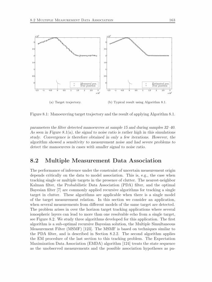
8.2 Multiple Measurement Data Association 163
−1.5 −1 −0.5 0 0.5 1 1.5 2 2.5 3
x 104
0
0.5
1
1.5
2
2.5
3
x 104
True positionMeasured pos.
(a) Target trajectory.
−1.5 −1 −0.5 0 0.5 1 1.5 2 2.5 3
x 104
0
0.5
1
1.5
2
2.5
3
x 104
True positionEstimated pos.
(b) Typical result using Algorithm 8.1.
Figure 8.1: Manoeuvring target trajectory and the result of applying Algorithm 8.1.
parameters the filter detected manoeuvres at sample 15 and during samples 32–40.As seen in Figure 8.1(a), the signal to noise ratio is rather high in this simulationsstudy. Convergence is therefore obtained in only a few iterations. However, thealgorithm showed a sensitivity to measurement noise and had severe problems todetect the manoeuvres in cases with smaller signal to noise ratio.
8.2 Multiple Measurement Data Association
The performance of inference under the constraint of uncertain measurement origindepends critically on the data to model association. This is, e.g., the case whentracking single or multiple targets in the presence of clutter. The nearest-neighborKalman filter, the Probabilistic Data Association (PDA) filter, and the optimalBayesian filter [7] are commonly applied recursive algorithms for tracking a singletarget in clutter. These algorithms are applicable when there is a single modelof the target measurement relation. In this section we consider an application,when several measurements from different models of the same target are detected.The problem arises in over the horizon target tracking applications where severalionospheric layers can lead to more than one resolvable echo from a single target,see Figure 8.2. We study three algorithms developed for this application. The firstalgorithm is a sub-optimal recursive Bayesian solution, the Multiple SimultaneousMeasurement Filter (MSMF) [123]. The MSMF is based on techniques similar tothe PDA filter, and is described in Section 8.2.2. The second algorithm appliesthe EM procedure of the last section to this tracking problem. The ExpectationMaximization Data Association (EMDA) algorithm [124] treats the state sequenceas the unobserved measurements and the possible association hypotheses as pa-

164 Target Tracking
Target
Platform
Ionospheric layers
Figure 8.2: The multiple measurement data association problem arises in over thehorizon target tracking.
rameters, this algorithm is detailed in Section 8.2.3. Finally, we apply the Gibbssampler of Chapter 6 to this association problem. The derivation of this MonteCarlo algorithm is provided in Section 8.2.4. The three algorithms are comparedthrough simulations of the tracking problem, presented in Section 8.2.5.
8.2.1 Problem Formulation
Consider a linear dynamical target state model
xt+1 = Ftxt +Gtwt, t = 0, 1, . . . (8.7)
where Ft ∈ Rnx×nx , and Gt ∈ Rnx×nu are known matrices, and wt is a zero meanwhite Gaussian sequence with known covariance Qt of full rank. At time t a set ofµt ≥ 0 measurements Yt = yi(t)µti=1 are detected, where each measurement eitheroriginate from one of n known linear measurement models or is a false detection,or clutter point. Explicitly, we let the received measurement be given by
yi(t) =
H1xt + e1(t) for model 1H2xt + e2(t) for model 2
......
Hnxt + en(t) for model nclutter otherwise
(8.8)
where yi(t) ∈ Rny and ei(t) is a white, zero mean Gaussian sequence with knowncovariance Ri of full rank. The sequences ei(t), i = 1, . . . , n are mutually indepen-dent and uncorrelated with the process noise wt. The algorithms presented belowadmit an explicitly known time variation in all system parameters. We refrainfrom introducing a known time variation in the measurement models, Hi(t), and

8.2 Multiple Measurement Data Association 165
Ri(t), solely to limit the notational complexity. Each measurement model in (8.8)produces a measurement with a probability PD, which for simplicity is assumedidentical for all n models. The number of clutter detections in each measurementset is Poisson distributed
pc(q) =(λVS)q
q!exp(−λVS) q = 0, 1, . . .
and the actual clutter measurements are uniformly distributed in the observationvolume, above labeled VS .
An explicit enumeration and description of all possible association events isneeded for sake of the trailing discussion. Denote a generic association event, orhypothesis, at time t by the µt-tuple
ψt = (i1, i2, . . . , iµt),
the indicator element ij is zero if the corresponding measurement yj(t) is supposedto be due to clutter, and a non-zero value, say q, indicates that yj(t) is due tomodel q, where 1 ≤ q ≤ µt. There is no repetition of nonzero elements in ψt, i.e.,we assume that a measurement can be due to at most one model. We also definethe target index set by Tt = j ∈ 1, 2, . . . , n : ij > 0. To exemplify, consider thecase of µt = 6 received measurements at time t and n = 3 measurement models.The association event ψt = (0, 0, 1, 0, 3, 0) would specify that measurement y3(t)originates from model number 1 and y5(t) originate from model number 3, whilethe remaining measurements are due to clutter. Model number 2 has failed todetect any measurements in this case and the target index set is Tt = 3, 5.
Let mt denote the number of measurements originating from the target, i.e.,the number of elements in Tt. The number of possible association hypotheses fora given number of mt target measurements follows by combinatorics as
rt(mt) =n!µt!
mt!(n−mt)!(µt −mt)!mt = 0, 1, . . . , νt (8.9)
where νtM= minµt, n. The total number of association hypotheses for the mea-
surement set received at time t is thus the sum
πt =νt∑
mt=0
rt(mt).
Hence, there are πt possible association events at time t. From (8.9) it is obviousthat the number of association events grows very fast with the number of receivedmeasurements. In the simulations presented in Section 8.2.5, we use n = 3 mea-surement models. Figure 8.3 shows the number of possible association hypothesesfor different numbers of received measurements. Receiving five or more measure-ments results in more than a hundred different association events, only at that timeinstant.
We introduce a generic enumeration of the πt association events, and let ψ(i)t
explicitly denote the ith association event. The number of target measurements,m
(i)t , and the target index set, T
(i)t , are defined correspondingly.

166 Target Tracking
1 2 3 4 5 6 7 80
100
200
300
400
500
600
Figure 8.3: The number of possible association events πt versus the number ofreceived measurements for the case of n = 3 measurement models.
8.2.2 Multiple Simultaneous Measurement Filter
Let ψ(i)t explictly denote the ith association event. The conditional filter density
of the states xt given the measurement set Yt = Yiti=0 is the mixture density
p(xt |Yt) =πt∑i=1
ci(t)p(xt |ψ(i)t ,Yt) (8.10)
where ci(t) is the association probability of event ψ(i)t ,
c(i)tM= Pr(ψ(i)
t |Yt), i = 0, 1, . . . , πt. (8.11)
Under each association hypothesis the conditional density is Gaussian, the optimalsolution consists of applying a Kalman filter to each hypothesis sequence. Thiswill lead to a mixture (8.10) where the number of terms grows exponentially withtime [7]. The MSMF [123] limits this growth by replacing the Gaussian mixturein (8.10) by a single Gaussian density at each algorithm iteration t in the spirit ofthe Probabilistic Data Association (PDA) filter [7].
Denote the conditional mean and covariance of the state by xt|t = E(xt |Yt)and Pt|t = Cov(xt |Yt). The recursive MSMF algorithm computes approximationsto this mean vector and covariance matrix, given by computing the first and secondcentral moments of (8.10),
xt|t =πt∑i=1
c(i)t x
(i)t|t (8.12a)
Pt|t =πt∑i=1
c(i)t
(P
(i)t|t + x
(i)t|t (x
(i)t|t )
T)− xt|txTt|t. (8.12b)
The state estimates x(i)t|t and error covariances P (i)
t|t are computed under the associ-ation event i at time t. Using the information form of the Kalman filter [2], they

8.2 Multiple Measurement Data Association 167
are determined by
x(i)t|t = xt|t−1 + P
(i)t|t
∑j∈T
(i)t
HTijR−1ij
(yj(t)−Hij xt|t−1) (8.13a)
(P (i)t|t )−1 = P−1
t|t−1 +∑j∈T
(i)t
HTijR−1ijHij . (8.13b)
The association probabilities (8.11) are given by the prior probability of the asso-ciation event and the likelihood of each Kalman filter,
c(i)t = κ−1 pc(µt −mt)PmtD (1− PD)n−mt
rt(mt)
∏j∈T
(i)t
N(yj(t);Hij xt|t−1, Sj)
Above, κ is a normalization constant, ensuring that∑πt
i=1 c(i)t = 1, mt is the number
of target measurements, and
Sj = HijPt|t−1HTij +Rij .
The MSMF given by Pulford and Evans [123] assumes that the full rank covariancestate noise enters purely additively in the estimation model, i.e., that Gt = I. Thissimplifies the algorithm since it ensures that P−1
t|t−1 exists and therefore enables theuse of the information form of the measurement updates in (8.13). This assump-tion can be removed, and the measurement update (8.13) can, e.g., be performedby sequential processing of the measurements in T
(i)t , see [2]. The time update
prediction of the estimate and error covariance is solved by a conventional Kalmanstep
xt+1|t = Ftxt|t
Pt+1|t = FtPt|tFTt +GtQtG
Tt
This completes one iteration of the recursive MSMF, a detailed derivation of thisrecursion is provided in [123].
8.2.3 Expectation Maximization Data Association
In the EMDA algorithm of Pulford and Logothetis [124], the complete batch ofmeasured data YN = Y (t)Nt=0 is considered for off-line processing and the EMalgorithm is applied to this estimation problem. The EMDA algorithm is obtainedby treating the target state sequence XN = xtNt=0 as the missing data and thesequence of association events ΨN = ψtNt=0 as the sought parameters. This yieldsthe EM iteration
Ψ(p+1)N = arg max
ΨNE(
log p(XN ,YN ,ΨN ) |YN , Ψ(p)N
)(8.14)
where expectation is performed with respect to the unobserved data XN .

168 Target Tracking
In [124], a target existence model is included which leads to dynamic program-ming via the Viterbi algorithm in the M-step of the EMDA algorithm. However,the target existence parameter introduces ambiguities into the estimator since thereexists no state sequence XN under the hypothesis that no target exists. Removingthe target existence model leads to an M-step that can be solved independently foreach t in the batch. To see this, we note that the density in (8.14) is recursivelyexpressed as
p(XN ,YN ,ΨN ) = p(YN |xN , ψN )p(xN |xN−1) Pr(ψN )p(XN−1,YN−1,ΨN−1),
and that terms independent of the association sequence not will affect the maxi-mization. Hence, we can use
Q(ΨN , Ψ(p)N ) = E
(N∑t=1
log p(Yt |xt, ψt) + log Pr(ψt)
∣∣∣∣∣YN , Ψ(p)N
)(8.15)
in liu of (8.14). This function can obviously be maximized independently for each tonce the expectation has been evaluated. The maximization of (8.15) is equivalentto maximizing for each t
Jp(ψt) = − 12
∑j∈Tt
‖yj(t)−Hij x(p)t|N‖
2
R−1ij
+mt log(ρ) + log Pr(ψt) (8.16)
where
ρ =VS√
(2π)ny(∏
j∈Tt|Rij |
) 1mt
, (8.17a)
Pr(ψt) = κ−1 pc(µt −mt)PmtD (1− PD)n−mt
rt(mt), (8.17b)
and x(p)t|N = E(xt |YN , Ψ(p)
N ) is obtained from a fixed interval Kalman smoother
under the hypothesis Ψ(p)N . In (8.17), mt is the number of target measurements,
and κ is a normalization constant ensuring that the probabilities sum to unity.Refer to [124] for a detailed derivation of these expressions.
In summary, the EMDA algorithm consists of the following steps
1. (Initialization p = 0)Choose an initial state sequence XN using the measurements YN . Set p := 1.
2. (M-step)Compute the measurement to target association Ψ(p)
N maximizing the costfunction (8.16) for each t = 0, 1, . . . , N using the state sequence X(p−1)
N .
3. (E-step)Compute the sequence of state estimates X(p)
N given the current associationsequence Ψ(p)
N using fixed interval Kalman smoothing.

8.2 Multiple Measurement Data Association 169
4. Set p := p+ 1 and return to item 2 above.
The iterations continue until no significant improvement is obtained during themaximization. The probability in (8.14) is by construction monotonically increas-ing with the number of passes through the EM-algorithm [8]. This ensures that alocal maxima of the density is reached and that the algorithm terminates.
8.2.4 Markov Chain Monte Carlo Data Association
The Markov chain Monte Carlo algorithm presented in this section has been devel-oped with inspiration from an application of similar ideas to estimation of parame-ters of jump-Markov linear systems by Doucet and Andrieu [61], Doucet et al. [62].Like the EMDA algorithm, we consider off-line batch processing of the collectedmeasurements YN , but here we propose to perform a Gibbs sampling procedureinstead.
1. Pick the initial association Ψ(0)N = ψ(0)
t Nt=0 randomly or deterministically.Set p = 1.
2. For each t = 0, 1, . . . , N generate a random sample from the full conditionaldistribution
ψ(p)t ∼ p(ψ(p)
t |YN ,Ψ(p)¬t ) (8.18)
3. Set p := p+ 1 and repeat at step 2.
The conditioning set in the full conditional (8.18) is
Ψ(p)¬t = Ψ(p)
t−1,Ψ(p−1)t+1:N = ψ(p)
0 , ψ(p)1 , . . . , ψ
(p)t−1, ψ
(p−1)t+1 , . . . , ψ
(p−1)N .
Discarding an initial burn-in phase, the sample average over the simulated out-put from this Gibbs sampler is a minimum mean square estimate of the associa-tion sequence. With this estimate of the association sequence at hand, a Kalmansmoother can be used to determine the states of the tracked system. Alternatively,Kalman smoothing can be performed between items 2 and 3, based on the sequenceΨ(p)N , and a Monte Carlo estimate of the state sequence formed from the smoothed
estimates.The full conditional distribution (8.18) is discrete with πt possible association
events at each time instant. In order to sample from this discrete distribution,we must calculate the full conditional probability for each association hypothesisconditioned on the previously drawn associations. This discrete full conditionaldistribution is given by
p(ψ(p)t |YN ,Ψ
(p)¬t ) =
p(YN |Ψ(p)¬t , ψ
(p)t ) Pr(ψ(p)
t )
p(YN |Ψ(p)¬t )
∝ p(YN |Ψ(p)¬t , ψ
(p)t ) Pr(ψ(p)
t ) (8.19)

170 Target Tracking
where the prior probabilities Pr(ψ(p)t ) are given by the model of the problem and
the number of received measurements at time t. Hence, the inner loop of the Gibbssampler relies on computing the likelihoods
p(YN |Ψ(p)¬t , ψ
(p)t = ψ
(i)t ) i = 1, . . . , πt. (8.20)
With these likelihood values at hand, the discrete distribution (8.19) is known upto a normalizing factor, and a sample can be generated from this distribution andinserted into Ψ(p)
¬(t+1) at the next iteration. Following Doucet and Andrieu [61],each iteration p of the Gibbs sampler is performed by a backward filtering forwardsampling procedure which has a complexity that is linear in the number of dataN . We proceed with a derivation of how to compute (8.20) using this efficientbackwards filtering forwards sampling scheme.
The likelihood (8.20) can be split into two parts
p(YN |Ψ(p)¬t , ψ
(p)t ) = p(Yt |Ψ(p)
¬t , ψ(p)t ) p(Yt+1:N |Ψ(p)
¬t , ψ(p)t ,Yt)
= p(Yt |Ψ(p)t ) p(Yt+1:N |Ψ(p−1)
t+1:N ,Ψ(p)t ,Yt).
Further decomposing the first factor and writing the second factor through amarginalization yields that the likelihood (8.20) equals
p(YN |Ψ(p)¬t , ψ
(p)t ) = p(Yt−1 |Ψ(p)
t−1) p(Yt |Yt−1,Ψ(p)t )∫
p(Yt+1:N , xt |Ψ(p−1)t+1:N ,Ψ
(p)t ,Yt) dxt.
Inserting this expression into (8.19) we have that
p(ψ(p)t |YN ,Ψ
(p)¬t ) ∝ p(Yt |Yt−1,Ψ
(p)t ) Pr(ψ(p)
t )∫p(Yt+1:N |Ψ(p−1)
t+1:N , xt) p(xt |Ψ(p)t ,Yt) dxt (8.21)
after removing the factors that are independent of ψ(p)t . Given the association
sequence Ψ(p)t , standard Kalman filter theory gives that
p(xt |Ψ(p)t ,Yt) = N(xt; xt|t, Pt|t) (8.22)
while
p(Yt |Yt−1,Ψ(p)t ) = N(Yt; Yt|t−1, St)
1V 1−mtS
is found from the innovation of this Kalman filter, and mt is the number of non-clutter observations under the hypothesis ψ(p)
t .We need an intermediate lemma in order to rewrite the last factor of (8.21).

8.2 Multiple Measurement Data Association 171
Lemma 8.2For any vectors Y , x, m, and matrices M , R, P of compatible dimensions∫
N(Y ;Mx,R) N(x;m,P ) dx = N(Y ;Mm,R+MPMT ) (8.23)
Proof Let Z ∼ N(0, R) and x ∼ N(m,P ) be independent Gaussian random vectors.Introduce Y = Z +Mx with probability density function p(Y ) =
∫p(Y |x)p(x)dx, given
by the left hand side of (8.23). On the other hand, Y is a linear combination of Gaussianvectors and obviously has probability density function p(Y ) = N(Y ;Mm,R + MPMT ).
Under a specific association hypothesis sequence Ψt+1:N , the considered data as-sociation problem is a standard linear state space problem, which yields that
Yt+1:N = Mtxt + Ut (8.24)
where
Mt =
Ht+1Ft
Ht+2Φt+1,t
...HNΦN−1,t
and
Ut =
Ht+1Gt 0 . . . . . 0
Ht+2Ft+1Gt Ht+2Gt+1 0 0...
. . ....0
HNΦN−1,t+1Gt . . . . . . . . . . . . . . . . . HNGN−1
wt
...wN−1
+
et+1
...eN
and we introduce the notation Φt+k,t = Ft+k . . . Ft+1Ft for the state transitionmatrix and Ht is the measurement matrix corresponding to generic association ψt.Hence,
Yt+1:N |Ψ(p−1)t+1:N , xt ∼ N(Mtxt, Lt)
where Lt = Cov(Ut) is positive definite by construction. From Lemma 8.2 we thushave that the last factor of (8.21) can be written as∫
p(Yt+1:N |Ψ(p−1)t+1:N , xt) p(xt |Ψ
(p)t ,Yt) dxt = N(Yt+1:N ;Mtxt|t, Lt +MtPt|tM
Tt )
(8.25)
where xt|t and Pt|t are computed under the hypothesis Ψ(p)t , as noted in (8.22). In
summary, the full conditional (8.21) is given by
p(ψ(p)t |YN ,Ψ
(p)¬t ) ∝ N(Yt; Yt|t−1, St) Pr(ψ(p)
t )V mtS
N(Yt+1:N ;Mtxt|t, Lt +MtPt|tMTt ) (8.26)

172 Target Tracking
where mt is the number of non-clutter measurements under ψ(p)t , as usual.
Next, we show how the last factor of (8.26) can be expressed through a backwards-forwards recursion. The matrix inversion lemma (4.A.20) gives that
(Lt +MtPt|tMTt )−1 = L−1
t − L−1t Mt(MT
t L−1t Mt + P−1
t|t )−1MTt L−1t ,
so the exponent of (8.25) can be decomposed according to
(Yt+1:N −Mtxt|t)T (Lt +MtPt|tMTt )−1(Yt+1:N −Mtxt|t) =
YTt+1:N L−1t Yt+1:N − 2xTt|tM
Tt L−1t Yt+1:N + xTt|tM
Tt L−1t Mtxt|t −
− (Yt+1:N −Mtxt|t)TL−1t Mt(MT
t L−1t Mt + P−1
t|t )−1MTt L−1t (Yt+1:N −Mtxt|t).
The first term in this expression is independent of the association event ψt and canthus be ignored. The determinant relation |I +AB| = |I +BA| yields that
|Lt +MtPt|tMTt | = |Lt||I + Pt|tM
Tt L−1t Mt|,
and since Lt is independent of the association event ψ(p)t the factor |Lt| can also
be ignored. Now, standard least squares estimation theory [2, 96] applied to (8.24)yields that the Fisher estimate of xt given Yt+1:N can be written
at|t+1M= P−1
t|t+1:N xt|t+1:N = MTt L−1t Yt+1:N
Γt|t+1M= P−1
t|t+1:N = MTt L−1t Mt,
Hence, running a backwards information filter under the hypothesis Ψ(p−1)N with
initial inverse covariance P−1N |N+1 = 0 will render the necessary quantities for com-
putation of the full conditional probabilities (8.26). The backwards informationfilter is given below, see, e.g., [80].
at|t = at|t+1 +HTt R−1t Yt (8.27a)
Γt|t = Γt|t+1 +HTt R−1t Ht (8.27b)
∆ =(GTt Γt|tGt +Q−1
t
)−1(8.27c)
at−1|t = FTt(I − Γt|tGt∆GTt
)at|t (8.27d)
Γt−1|t = FTt(I − Γt|tGt∆GTt
)Γt|tFt (8.27e)
for t = N,N − 1, . . . , 1. The Fisher estimates are obtained by initializing the filterwith
ΓN |N+1 = 0 and aN |N+1 = 0. (8.27f)
The backwards information filter sequence is computed under the association hy-pothesis Ψ(p−1)
N . Thus, Yt in (8.27a) is the stacked vector of non-clutter measure-ments under the hypothesis ψ(p−1)
t , and Ht and Rt are the corresponding measure-ment equation matrix and measurement error covariance, respectively.

8.2 Multiple Measurement Data Association 173
Collecting the results above yields that the full conditional probability (8.19) isgiven by
p(ψ(p)t |YN ,Ψ
(p)¬t ) ∝ N(Yt; Yt|t−1, St)
pc(µt −mt)PmtD (1− PD)n−mtV mtS
rt(mt)×
|I + Pt|tΓt|t+1|−1/2 exp(− 1
2‖xt|t‖2
Γt|t+1+ xTt|tat|t+1+
12‖at|t+1 − Γt|t+1xt|t‖2(Γt|t+1+P−1
t|t )−1
), (8.28)
where Yt|t−1, xt|t, and Pt|t are based on ψ(p)t . It may require to use the matrix
inversion lemma on the last term in the exponent of (8.28), and set
(Γt|t+1 + P−1t|t )−1 = Pt|t − Pt|tΓt|t+1(Pt|tΓt|t+1 + I)−1Pt|t
whenever Pt|t is singular. One iteration of the Gibbs sampler based on (8.28) canthus be computed using an initial backwards information filtering sweep, followedby a forwards sampling iteration that determines the association sequence andsequentially runs a Kalman filter based on this sequence. We label this algorithmthe Monte Carlo Data Association (MCDA) algorithm.
Algorithm 8.2 (Monte Carlo Data Association (MCDA))
1. Initialize by picking the initial association Ψ(0)N randomly or deterministically.
Set p = 1.
2. Run the backwards information filter (8.27) using Ψ(p−1)N . Store Γt|t+1 and
at|t+1.
3. Initialize the Kalman filter quantities x0|−1 and P0|−1, set t = 0, and computethe following forward recursion:
(a) Run Kalman filter measurement updates under each possible associationhypothesis for Yt, i.e., for k = 1, . . . , πt. Store every xkt|t and P kt|t.
(b) Compute (8.28) under all πt hypotheses, normalize this discrete density,and generate a sample from this discrete distribution,
ψ(p)t ∼ p(ψ(p)
t |YN ,Ψ(p)¬t ).
(c) Set t := t+1, run a time update step with the Kalman filter correspondingto the chosen association, store the resulting xt+1|t and Pt+1|t and usethem in the next iteration at item 3(a). If t > N , go to item 4 instead.
4. Compute X(p)N = E
(XN |YN ,Ψ(p)
N
)by fixed interval Kalman smoothing.
5. Output the association sequence Ψ(p)N and the state sequence X(p)
N . Set p :=p+ 1 and return to item 2.

174 Target Tracking
The algorithm above is iterated M times, and minimum mean square estimates ofthe state and association sequences are formed according to
XN =1M
M∑i=1
X(i)N ΨN =
1M
M∑i=1
Ψ(i)N ,
possibly after discarding an initial burn-in phase of the algorithm. The associationestimate above should be interpreted as a weighted average over some numbering ofthe hypotheses, possibly followed by a conversion to integer estimates afterwards.
The backwards filtering computation in item 2 of Algorithm 8.2 can actually beretained from the calculations in item 4 by utilizing a specific type of smoothingformula [96]. Mayne [115] formulated the linear smoothing problem as an optimiza-tion problem, decomposed into one minimization with respect to past data, andone with respect to future data. Fraser and Potter [69] later suggested that thisapproach could be interpreted as the combination of two optimal filters: one back-wards information filter (8.27), and one regular forward Kalman filter. Let xt|t−1
and Pt|t−1 be one step ahead predictions from a standard Kalman filter appliedunder the same association hypothesis as used in (8.27). The smoothed estimatext|N is computed by combining the quantities xt|t−1 and Pt|t−1 with the resultsof (8.27),
xt|N =(I − PtΓt|t(PtΓt|t + I)−1
)(xt|t−1 − Ptat|t),
see [69, 96]. The estimates produced by a backwards information filter at item 4can thus be reused at item 2 in the next iteration of the MCDA algorithm.
Algorithm 8.2 can straightforwardly be utilized for MAP, or marginal MAPestimation as well. A simulated annealing algorithm is obtained by sampling from
p(ψ(p)t |YN ,Ψ
(p)¬t )
1Tp
where Tp is a cooling sequence in the sense described in Chapter 6. Alternativelythe maximization can be performed deterministically by picking the associationthat maximizes the full conditional at each iteration, see [61] for similar ideas.
8.2.5 Simulation Result
The simulations follow the setup described in [123]. The target state consists ofrange, rt, azimuth, θt, and their respective time derivatives, xt = (rt, rt, θt, θt)T .The true target state trajectory obeys
rt = 50 + 5tT rt = 5
θt = 0.3tT θt = 0.3
with t = 0, 1, . . . , 15 and sampling time T = 2. Three measurement models wereused,
Hi =
1 + i−110 0 0 0
0 1 0 00 0 1 0
for i ∈ 1, 2, 3,

8.2 Multiple Measurement Data Association 175
all having identical noise covariance
R =
102 0 00 0.12 00 0 52
The state noise covariance and initial state covariance used in the filters was set to
Q =
0.1 0 0 00 0.1 0 00 0 0.0125 00 0 0 0.0125
and P0 =
200 0 0 00 1 0 00 0 1 00 0 0 1
The observation volume VS was defined by
25 ≤ rt ≤ 2254.5 ≤ rt ≤ 5.5 (8.29)−2 ≤ θt ≤ 10.
Figure 8.4 shows a simulation case with high probability of correct measurementdetection, PD = 0.95, and low clutter intensity, λVS = 0.4. In the figure, solid lines
0 10 20 30
0
50
100
150
200
Range
0 10 20 304
4.5
5
5.5
6
6.5Range rate
0 10 20 30−5
0
5
10Azimuth
0 10 20 30−4
−2
0
2
4
(not measured)
Azimuth rate
Figure 8.4: Simulation case, PD = 0.95, λVS = 0.4.
show the true target states, pluses indicate measurements origin from the target,and squares indicate clutter points. The typical performance of the algorithms areshown in Figures 8.5–8.7. In all figures, the asterisk (∗) indicate the true target statevalue, the solid line is the estimate, and the dotted line is the ±3σ confidence regionof the estimate. The first measurement was used for initialization of the algorithms.The transients in the MSMF estimates in Figure 8.5 stem from two clutter pointsin the measurement used for initialization. The iterative passes in the EMDA filter

176 Target Tracking
0 10 20 30−50
0
50
100
150
200Range
0 10 20 304
4.5
5
5.5
6
6.5Range rate
0 10 20 30−5
0
5
10Azimuth
0 10 20 30−4
−2
0
2
4Azimuth rate
Figure 8.5: Performance of MSMF, PD = 0.95, λVS = 0.4.
0 10 20 30−50
0
50
100
150
200Range
0 10 20 304
4.5
5
5.5
6
6.5Range rate
0 10 20 30−5
0
5
10Azimuth
0 10 20 30−4
−2
0
2
4Azimuth rate
Figure 8.6: Performance of EMDA, PD = 0.95, λVS = 0.4.
manage to compute an almost perfect association, with resulting state estimatesdepicted in Figure 8.6. The EMDA algorithm converges in less than five iterationsin this simulation study, but has considerably higher computational complexitythan the MSMF. The results using the MCDA algorithm are shown in Figure 8.7.Since the state estimates of this algorithm are computed by Monte Carlo estimation,no state covariance is available and therefore there are no confidence regions shownin Figure 8.7. The estimates depicted in the figure are the resulting Monte Carloestimates obtained when running M = 5 iterations of the MCDA algorithm, andregarding only the initial iteration as a burn-in sample. The computations requiredto perform one iteration of the MCDA algorithm exceed the computations of the

8.2 Multiple Measurement Data Association 177
0 10 20 30−50
0
50
100
150
200Range
0 10 20 304
4.5
5
5.5
6
6.5Range rate
0 10 20 30−5
0
5
10Azimuth
0 10 20 30−4
−2
0
2
4Azimuth rate
Figure 8.7: Performance of MCDA, PD = 0.95, λVS = 0.4.
EMDA and the MSMF.A second simulation case with less frequent real measurements and more clut-
ter is depicted in Figure 8.8. In these simulations, on the average two clutter
0 10 20 30
0
50
100
150
200
Range
0 10 20 304
4.5
5
5.5
6
6.5Range rate
0 10 20 30−5
0
5
10Azimuth
0 10 20 30−4
−2
0
2
4
(not measured)
Azimuth rate
Figure 8.8: Simulation case, PD = 0.5, λVS = 2.
measurements are received in each measurement set, and only half of the real mea-surement models generate observations. The simulation results obtained with thedata in Figure 8.8 are shown in Figure 8.9–8.11. The MSMF filter has greaterproblems with this dense clutter case, as shown in Figure 8.9. The EMDA algo-rithm in Figure 8.10 still yields very accurate range estimates while the range rateis less precise. The MCDA performance in Figure 8.11 is almost identical to the

178 Target Tracking
0 10 20 30−50
0
50
100
150
200Range
0 10 20 304
4.5
5
5.5
6
6.5Range rate
0 10 20 30−5
0
5
10Azimuth
0 10 20 30−4
−2
0
2
4Azimuth rate
Figure 8.9: Performance of MSMF, PD = 0.5, λVS = 2.
0 10 20 30−50
0
50
100
150
200Range
0 10 20 304
4.5
5
5.5
6
6.5Range rate
0 10 20 30−5
0
5
10Azimuth
0 10 20 30−4
−2
0
2
4Azimuth rate
Figure 8.10: Performance of EMDA, PD = 0.5, λVS = 2.
one obtained for the case with less clutter points and more target measurements.The results in Figure 8.11 are computed from a ten iteration run of the MCDAalgorithm, discarding the chain output for the initial four iterations.
8.3 Conclusion
In the multiple measurement data association problem, the number of possibleassociation hypotheses may reach very high levels. We have studied three statis-tical algorithms for this joint measurement association and state estimation prob-

8.3 Conclusion 179
0 10 20 30−50
0
50
100
150
200Range
0 10 20 304
4.5
5
5.5
6
6.5Range rate
0 10 20 30−5
0
5
10Azimuth
0 10 20 30−4
−2
0
2
4Azimuth rate
Figure 8.11: Performance of MCDA, PD = 0.5, λVS = 2.
lem. The recursive Multiple Simultaneous Measurement Filter (MSMF) mergesthe hypotheses at each time iteration, while the Expectation Maximization DataAssociation (EMDA) applies the EM algorithm for MAP estimation of the asso-ciation sequence, regarding a batch of the state sequence as unobserved data. Anovel Gibbs sampling algorithm for batch processing has been developed for thisproblem. The Monte Carlo Data Association (MCDA) algorithm has a backwardfiltering, forward sampling structure and can be utilized to yield either MMSE orMAP estimates of the state and association sequences.
The batch algorithms EMDA and MCDA show superior performance over therecursive MSMF procedure. The primitive initialization used in the simulationsdegrades the performance of the MSMF considerably when there is clutter in themeasurement set. With a more elaborate initialization this effect could perhapsbe attenuated. The MSMF would also gain in accuracy with the introduction ofmeasurement gating [7]. Neither the EMDA nor the MCDA seems to suffer fromthe initialization problems, though. These algorithms yield reliable state estimates,even in the simulation case of very dense clutter.

Appendix
8.A Expectation Maximization for Segmentation
This appendix contains a derivation of the EM algorithm for segmentation pre-sented in Section 8.1.1.
We introduce the stacked stacked vectors of N random variables from (8.2)
X = [xT1 , xT2 , . . . , x
TN ]T U = [xT1 , w
T1,δ, . . . , w
TN−1,δ]
T
E = [eT1,δ, eT2,δ, . . . , e
TN,δ]
T
where the noise vectors U and E explicitly depend on the segmentation sequence∆. Using this notation, the estimation model (8.2) can be written compactly as
X = A∆UY = B∆X+ E
(8.A.30)
where matrices A∆ and B∆ are block matrices formed by the state space matricesof the model (8.2). Direct inspection yields that
A∆=
I 0 . . . . . . . . . . . . . . . 0W 1
1 I 0 . . . . . . . . . . 0W 2
1 W 22 I 0 . . . . . . 0
.... . .
...0
WN−11 . . . . . . . . . . . . WN−1
N−1 I
I 0 . . . . . . . . . . . . . . . 00 G1,δ 0 . . . . . . . . 00 0 G2,δ 0 . . . 0...
. . ....0
0 . . . . . . . . . . . . . . . . . . 0 GN−1,δ
where zeros denote zero matrices of appropriate dimension, and the state transitionmatrix is defined as
W lt = Fl,δFl−1,δ · · ·Ft,δ.
Furthermore,
B∆ = diag(H1,δ, H2,δ, . . . , HN,δ)
180

8.A Expectation Maximization for Segmentation 181
where diag(A1, A2, . . . , AM ) denotes a matrix with blocks Ai along the diagonal.The statistical properties of the noises in (8.A.30) are compactly given in the ex-pression
E
[UE
] [UT ET 1
]=[Q∆ 0
[x10
]0 R∆ 0
](8.A.31)
where both Q∆ and R∆ are block diagonal,
Q∆ = diag (P1, Q1,δ, Q2,δ, . . . , QN−1,δ)R∆ = diag (R1,δ, R2,δ, . . . , RN,δ) .
Eliminating the states X in (8.A.30) yields
Y = B∆A∆U+ E. (8.A.32)
In the EM algorithm of Section 8.1.1, we treat the segmentation sequence ∆ as theparameters and the vector U as the unobserved data in the model (8.A.32). Witha Bayesian framework each EM pass p is defined by
∆p+1 = arg max∆
E (log p(Y,U,∆) |Y,∆p) (8.A.33)
where the joint density can be divided into three factors
p(Y,U,∆) = p(Y |U,∆)p(U |∆)p(∆). (8.A.34)
The first and second factors are given by (8.A.32) and (8.A.31) above,
p(Y |U,∆) = N (Y;B∆A∆U, R∆)
p(U |∆) = N(U;[x10
], Q∆
).
The last factor is the Bayesian prior for the segmentation sequence.Denoting the quadratic norm xTAx by ‖x‖2A, and the determinant by |A|, the
logarithm of (8.A.34) is
log p(Y,U,∆) = log p(∆)− 12‖Y−B∆A∆U‖2R−1
∆− 1
2 log |R∆| − 12 log |Q∆| −
− 12‖U−
[x10
]‖2Q−1
∆− (N−1)nu+Nny+nx
2 log(2π). (8.A.35)
Since the maximization in (8.A.33) is performed over the segmentation sequence ∆only terms involving the segmentation parameters need to be retained from (8.A.35)when the conditional expectation is evaluated. Hence, removing terms and positivefactors independent of the segmentation sequence we define the return function
J(Y,U,∆) = 2 log p(∆)− ‖Y−B∆A∆U‖2R−1∆− log |R∆| − log |Q∆| −
− ‖U−[x10
]‖2Q−1
∆(8.A.36)

182 Target Tracking
and use the auxiliary function
Q(∆,∆p) = EU (J(Y,U,∆) |Y,∆p) .
The conditional mean and covariance of the vector U, given by
Up = E (U |Y,∆p)
Sp = E(
(U− Up)(U− Up)T |Y,∆p
),
(8.A.37)
can be obtained using standard linear estimation theory on the model (8.A.32)after inserting the segmentation sequence ∆p. Taking the conditional expectationof (8.A.36), inserting (8.A.37) and completing the squares yield
Q(∆,∆p) = 2 log p(∆)− ‖Y−B∆A∆Up‖2
R−1∆− log |R∆| − log |Q∆| −
− ‖Up −[x10
]‖2Q−1
∆− tr
((AT∆B
T∆R−1∆ B∆A∆ +Q−1
∆
)Sp)
(8.A.38)
where the linearity of the trace operator tr(·) and the relation ‖x‖2A = tr(AxxT )has been used repeatedly.
Standard fixed interval linear state smoothing can be used to compute thereturn (8.A.38). Define a notation for the conditional mean and covariance of thecomplete state sequence
Xp = E (X |Y,∆p)
Pp = E(
(X− Xp)(X− Xp)T |Y,∆p
).
(8.A.39)
From (8.A.30) we have that
X = A∆U U = A†∆X
where M † = (MTM)−1MT is the Moore-Penrose pseudo inverse. Inserting thisinto the return (8.A.36) yields
J(Y,X,∆) = 2 log p(∆)− ‖Y−B∆X‖2R−1∆− log |R∆| − log |Q∆| −
− ‖A†∆X−[x10
]‖
2
Q−1∆
taking conditional expectation, inserting (8.A.39) and completing the squares wehave that
Q(∆,∆p) = 2 log p(∆)− ‖Y−B∆Xp‖2
R−1∆− log |R∆| − log |Q∆| −
− ‖A†∆Xp −[x10
]‖2Q−1
∆− tr
((BT∆R
−1∆ B∆ +A†T∆ Q−1
∆ A†∆
)Pp). (8.A.40)

8.A Expectation Maximization for Segmentation 183
It is straightforward to verify that the pseudo inverse of A∆ has a strong diagonalstructure,
A†∆ =
I 0 . . . . . . . . . . . . . . . . . . . . . . . . . . . . . 0−G†1,δF1,δ G†1,δ 0 . . . . . . . . . . . . . . . . . . . . . . 0
0 −G†2,δF2,δ G†2,δ 0 . . . . . . . . . . . . . . . . . . . 0...
...0
0 . . . . . . . . . . . . . . . . . . . 0 −G†N−1,δFN−1,δ G†N−1,δ
.
Furthermore, B∆, R−1∆ and Q−1
∆ are all block diagonal which means that each normand matrix trace in (8.A.40) can be written as a sum of norms and matrix tracesof smaller matrices. Introducing a notation for the smoothed state estimate and(cross) covariance
xpt = E (xt |Y,∆p)
P pl,t = E((xl − xpl )(xt − x
pt )T |Y,∆p
),
it follows that the return function (8.A.40) can be written
Q(∆,∆p) =N∑t=1
(2δt log
(1−qq
)− ‖yt −Ht,δx
pt ‖
2
R−1t,δ− tr
(HTt,δR
−1t,δHt,δP
pt,t
)−
− log |Rt,δ|)−N−1∑t=1
(‖G†t,δ(x
pt+1 − Ft,δx
pt )‖
2
Q−1t,δ
+ log |Qt,δ|+
tr(G†Tt,δQ
−1t,δG
†t,δ(P
pt+1,t+1 − 2Ft,δP
pt,t+1 + Ft,δP
pt,tF
Tt,δ)))
, (8.A.41)
where the terms independent of ∆ have been removed from the expression, and theBernoulli prior (8.4),
log p(∆) =N∑t=1
δt log(
1−qq
),
has been inserted.

184 Target Tracking

9
Conclusive Remarks
The Bayesian paradigm for statistical inference yields a natural framework forrecursive nonlinear estimation problems. All information gained about the statesfrom initial to present time is in this framework condensed by the posterior filterdensity. The conceptual recursive update of the posterior density is simple instructure, yet impossible to implement when then problem is of nonlinear andnon-Gaussian character.
The pure notion of the existence of the optimal solution is valuable in the huntfor high performing algorithms. Rather than blindly turn to model approxima-tions, we propose to utilize the conceptual update and approximately implementit as efficiently as possible, e.g., using a point-mass approach. The main differencebetween model and solution approximations is that in the latter scheme, it is pos-sible to obtain a graceful degradation of the optimal solution. A tradeoff betweenestimation accuracy and implementational complexity is found by controlling thegrid mesh resolution in a numerical implementation.
The Bayesian approach to recursive estimation has proven to be utterly suc-cessful for the terrain navigation application. The results from the work on thisapplication shows that complex problems of this type can be handled with greatsuccess using approximative Bayesian inference. The point-mass implementationhas shown to yield high performance in the terrain navigation application, both onsimulated but realistic measurements and on actual field test data. One of the fu-ture challenges for this application is to maximize the utilization of the point-mass
185

186 Conclusive Remarks
description for the integration with the inertial navigation system.The Cramer-Rao bounds to recursive estimation provides an appealing ap-
proach to evaluation of suboptimal algorithms. The recursive expressions forCramer-Rao bounds to nonlinear filtering has provided us with arguments that thesuboptimal point-mass implementation of the terrain navigation application hasnear optimal performance. The way we estimate both the bounds and the algo-rithm performance in Monte Carlo simulations have shown to yield a concrete toolfor verification of suboptimal algorithms. Both the parametric and the Bayesian,i.e., posterior, bounds can be utilized in such Monte Carlo evaluations.
Practical implementation of recursive Bayesian estimation problems has shownto be tightly connected to function approximation and numerical integration. Ageneral combination of these concepts was pursued in the ideas outlined about awavelet multiresolution approach to spatial grid adaption. Even though a greatdeal of time has been spent on investigations into this approach, the resultingconclusion from this work is rather discouraging and the concepts are only givenminor space in this presentation. Guidelines about adaptive grid methods for gen-eral nonlinear recursive estimation will inevitably be very hard to set. We believethat each recursive estimation problem should instead be investigated and solvedwith the methods best suited for that application. In some cases, an adaptivemesh will prove useful, in others a uniform mesh will suffice. The wavelet multires-olution techniques provides a uniform approach to function approximation andnumerical integration. However, the implementational difficulties are currently toooverwhelming for pursuing this approach in a practical application.
The Monte Carlo filters rely on a straightforward simulation strategy to deter-mine a spatially adaptive grid, well suited for the problem at hand. The particlefilters are simple in structure and demand no design of a grid mesh propagation orresampling scheme. In the comparative simulations of the terrain navigation ap-plication we have seen that the particle filters and the point-mass approach reachthe same level of performance. Future work will involve applying the particle fil-ters to terrain navigation when the absolute altitude is biased, or directly to theintegration of inertial navigation and terrain navigation.
Simulation based methods for recursive estimation is currently a very activeresearch field which interests both pure statisticians and people form the field ofsignal processing. Different approaches to enhance the performance of the basicparticle filters are constantly appearing in the literature. One main advantagewith the simulation based algorithms is their ease of implementation. They alsoextend to higher dimensional problems with only minor implementational effort.We believe that these issues will make the basic Monte Carlo filters reviewed inthis work the future workhorses of nonlinear recursive estimation.

Bibliography
[1] D.L. Alspach and H.W. Sorenson. Nonlinear Bayesian estimation using Gaus-sian sum approximation. IEEE Transactions on Automatic Control, 17:439–448, 1972.
[2] B.D.O. Anderson and J.B. Moore. Optimal Filtering. Prentice Hall, Engle-wood Cliffs, NJ, 1979.
[3] C. Andrieu, A. Doucet, and P. Duvaut. Joint Bayesian detection and estima-tion of sinusoids embedded in noise. In Proc. IEEE Conf. Acoustics, Speechand Signal Processing (ICASSP), 1998.
[4] C. Andrieu, A. Doucet, S.J. Godsill, and W.J. Fitzgerald. An introductionto the theory and applications of simulation based computational methodsin Bayesian signal processing. Technical Report CUED/F-INFENG/TR.324,Department of Engineering, University of Cambridge, UK, 1998.
[5] D. Avitzour. Stochastic simulation Bayesian approach to multitarget track-ing. IEE Proc. on Radar, Sonar and Navigation, 142(2), 1995.
[6] W. Baker and R. Clem. Terrain contour matching [TERCOM] primer.Technical Report ASP-TR-77-61, Aeronautical Systems Division, Wright-Patterson AFB, Aug. 1977.
187

188 Bibliography
[7] Y. Bar-Shalom and T. Fortmann. Tracking and Data Association, volume179 of Mathematics in Science and Engineering. Academic Press, 1988.
[8] L.E. Baum, T. Petrie, G. Soules, and N. Weiss. A maximization techniqueoccuring in the statistical analysis of probabilistic functions of Markov chains.The Annals of Mathematical Statistics, 41:164–171, 1970.
[9] T.R. Bayes. An essay towards solving a problem in the doctrine of chances.Phil. Trans. Roy. Soc. London, 53(370), 1763. Reprinted in Biometrica,45(293), 1958.
[10] E.R. Beadle and P.M. Djuric. A fast weighted Bayesian bootstrap filterfor nonlinear model state estimation. IEEE Transactions on Aerospace andElectronic Systems, 33(1):338–343, 1997.
[11] E.R. Beadle and P.M. Djuric. Parameter estimation for non-Gaussian au-toregressive processes. In Proc. IEEE Conf. Acoustics, Speech and SignalProcessing (ICASSP), 1997.
[12] E.R. Beadle and P.M. Djuric. Uniform random parameter generation of stableminimum-phase real ARMA (p, q) processes. IEEE Signal Processing Letters,4(9), 1997.
[13] V.E. Benes. Exact finite-dimensional filters for certain diffusions with non-linear drift. Stochastics, 5:65–92, 1981.
[14] J.O. Berger. Statistical Decision Theory and Bayesian Analysis. Springer-Verlag, 2nd edition, 1985.
[15] N. Bergman. A Bayesian approach to terrain-aided navigation. In Proc. ofSYSID’97, 11th IFAC Symposium on System Identification, pages 1531–1536.IFAC, 1997.
[16] N. Bergman. Bayesian Inference in Terrain Navigation. Linkoping Studiesin Science and Technology. Thesis No 649, 1997.
[17] N. Bergman. On the Cramer-Rao bound for terrain-aided navigation.Technical Report LiTH-ISY-R-1970, Department of Electrical Engineering,Linkopings University, 1997.
[18] N. Bergman. Deterministic and stochastic Bayesian methods in terrain nav-igation. In Proc. 37:th IEEE Conf. on Decision and Control, 1998.
[19] N. Bergman. Expectation maximization segmentation. Technical ReportLiTH-ISY-R-2067, Department of Electrical Engineering, Linkoping Univer-sity, 1998.
[20] N. Bergman. An interpolating wavelet filter for terrain navigation. InProc. conf. on multisource-multisensor information fusion, pages 251–258,1998.

Bibliography 189
[21] N. Bergman. Terrain navigation using sequential Monte Carlo methods. InA. Doucet, J.F.G. de Freitas, and N.J. Gordon, editors, Sequential MonteCarlo methods in practice. Cambridge University Press, 1999. To appear.
[22] N. Bergman and F. Gustafsson. Three statistical batch algorithms for track-ing manoeuvring targets. In Proc. 5th European Control Conference, Karl-sruhe, Germany, 1999.
[23] N. Bergman, L. Ljung, and F. Gustafsson. Point-mass filter and Cramer-Raobound for terrain-aided navigation. In Proc. 36:th IEEE Conf. on decisionand control, pages 565–570, 1997.
[24] N. Bergman, L. Ljung, and F. Gustafsson. Terrain navigation using Bayesianstatistics. IEEE Control Systems Magazine, 19(3), June 1999.
[25] N. Bergman and P. Tichavsky. Two Cramer-Rao bounds for terrain-aidednavigation. IEEE Transactions on Aerospace and Electronic Systems, 1999.In review.
[26] G. Beylkin. On the fast algorithm for multiplication of functions in thewavelet bases. Technical report, Prog. in Appl. Math., Univ. of Colorado atBoulder, Boulder, CO 80309-0526, jun 1992.
[27] G. Beylkin. Wavelets and fast numerical algorithms. In I. Daubechies, editor,Different Perspectives on Wavelets, volume 47 of Proceedings of Symposia inApplied Mathematics, pages 89–117. American Math. Soc., Providence, RI,1993. From an American Math. Soc. short course, Jan. 11–12, 1993, SanAntonio, TX.
[28] G. Beylkin, R. Coifman, and V. Rokhlin. Fast wavelet transforms and nu-merical algorithms. Comm. in Pure and Applied Math., 44:141–183, 1991.
[29] S.S. Blackman. Multiple-target tracking with radar applications. ArtechHouse, Norwood, MA, 1986.
[30] E. Bølviken, P.J. Acklam, N. Christophersen, and J-M Størdal. Monte Carlofilters for non-linear state estimation. Technical report, University of Oslo,1997.
[31] D. Boozer and J. Fellerhoff. Terrain-Aided Navigation Test Results in theAFTI/F-16 Aircraft. Journal of The Institute of Navigation, 35(2):161–175,Summer 1988.
[32] B.Z. Borobsky and M. Zakai. A lower bound on the estimation error forMarkov processes. IEEE Transactions on Automatic Control, 20(6):785–788,1975.
[33] G. Box and G. Tiao. Bayesian Inference in Statistical Analysis. John Wiley,1992.
190 Bibliography
[34] R.S. Bucy and K.D. Senne. Digital synthesis of nonlinear filters. Automatica,7:287–298, 1971.
[35] D.M. Buende and P. Girardi. A target identification comparison of Bayesianand Dempster-Shafer multisensor fusion. IEEE Tr. Man and Cybernetics, 27(5):569–577, 1997.
[36] Z. Cai, F. Le Gland, and H. Zhang. An adaptive local refinement method fornonlinear filtering. Technical Report No 2679, Unite de rechereche INRIARennes, 1995.
[37] J. Carpenter, P. Clifford, and P. Fearnhead. An improved particle filter fornon-linear problems. In IEE Proceedings on Radar and Signal Processing,1998. In press.
[38] J. Carpenter, P. Clifford, and P. Fearnhead. Building robust sumilation-basedfilters for evolving data sets. Technical report, Department of Statistics,University of Oxford, 1999.
[39] H. Carvalho, P. Del Moral, A. Monin, and G. Salut. Optimal nonlinear filter-ing in GPS/INS integration. IEEE Transactions on Aerospace and ElectronicSystems, 33(3), 1997.
[40] K.L. Chung. A course in probability theory. Academic Press, 1968.
[41] D. Crisan, P. Del Moral, and T. Lyons. Discrete filtering using branching andinteracting particle systems. Technical Report 1-98, Laboratoire de Statis-tique et Probabilites, Universite Paul Sabatier, Toulouse, 1998.
[42] I. Daubechies. Ten Lectures on Wavelets. SIAM, 1992.
[43] F.E. Daum. New exact nonlinear filters. In J.C. Spall, editor, Bayesian Anal-ysis of Time Series and Dynamic Models, volume 94 of Statistics, textbooksand monographs, chapter 8, pages 199–226. Marcel Dekker inc., New York,1988.
[44] P. Davies. The F-16 digital terrain system. In IEE 1995 Colloquium onTerrain databases and their use in navigation and collision avoidance. IEE,1995.
[45] P.J. Davis and P. Rabinowitz. Numerical Integration. Blaisdell PublishingCompany, 1967.
[46] P.J. Davis and P. Rabinowitz. Methods of Numerical Integration. AcademicPress, 2nd edition, 1984.
[47] R.J.P. de Figueiredo and Y.G. Jan. Spline filters. In Proc. 2nd symp. onnonlinear estimation theory and its applications, pages 127–138, 1971.

Bibliography 191
[48] J.F.G. de Freitas, M. Niranjan, A.H. Gee, and A. Doucet. Sequential MonteCarlo methods for optimization of neural network models. Technical Re-port CUED/F-INFENG/TR.324, Department of Engineering, University ofCambridge, UK, 1998.
[49] P. Del Moral. Measure-valued processes and interacting particle systems. Ap-plication to nonlinear filtering problems. The Annals of Applied Probability,8(2):438–495, 1998.
[50] A.P. Dempster. New methods for reasoning towards posterior distributionsbased on sample data. Ann. Math. Stat., 34:355–374, 1966.
[51] A.P. Dempster. Upper and lower probabilites induced by a multivalued map-ping. Ann. Math. Stat., 38:325–339, 1967.
[52] A.P. Dempster. A generalization of Bayesian inference. Journal of the RoyalStatistical Society, 30:202–247, 1968.
[53] A.P Dempster, N.M. Laird, and D.B. Rubin. Maximum likelihood from in-complete data via the EM algorithm. Journal of the Royal Statistical Society,pages 1–38, 1977.
[54] G. Deslauriers and S. Dubuc. Symmetric iterative interpolation processes.Constructive Approximation, 5(1):49–68, 1989.
[55] P.M. Djuric, S.J. Godsill, W.J. Fitzgerald, and P.J.W. Rayner. Detectionand estimation of signals by reversible jump Markov chain Monte Carlo com-putations. In Proc. IEEE Conf. Acoustics, Speech and Signal Processing(ICASSP), 1998.
[56] P.C. Doerschuk. Cramer-Rao bounds for discrete-time nonlinear filteringproblems. IEEE Transactions on Automatic Control, 40(8):1465–1469, 1995.
[57] D.L. Donoho. De-noising by soft-thresholding. Technical Report 409, Dept.of Statistics, Stanford University, 1992.
[58] D.L. Donoho. Interpolating wavelet transforms. Technical Report 408, Dept.of Statistics, Stanford University, 1992.
[59] D.L. Donoho. Smooth wavelet decompositions with blocky coefficient ker-nels. In L.L. Shumaker and G. Webb, editors, Recent Advances in WaveletAnalysis, pages 259–308. Academic Press, New York, 1993.
[60] A. Doucet. On sequential simulation-based methods for Bayesian filtering.Technical Report CUED/F-INFENG/TR.310, Signal Processing Group, De-partment of Enigeering, University of Cambridge, 1998.
[61] A. Doucet and C. Andrieu. Iterative algorithms for state estimation of jumpMarkov linear systems. IEEE Transactions on Signal Processing, 1999. Inreview.

192 Bibliography
[62] A. Doucet, A. Logothetis, and V. Krishnamurthy. Stochastic sampling al-gorithms for state space estimation of jump Markov linear systems. IEEETransactions on Automatic Control, 1999. Accepted for publ.
[63] R.J. Elliott, L. Aggoun, and J.B. Moore. Hidden Markov Models – Estimationand Control. Springer Verlag, 1997.
[64] R. Enns and D. Morrell. Terrain-aided navigation using the Viterbi algorithm.Journal of Guidance, Control and Dynamics, 18(6):1444–1449, November-December 1995.
[65] J. Evans and V. Krishnamurthy. Optimal filtering of doubly stochastic auto-regressive processes. Automatica, 35(2):241–250, 1999.
[66] P. Fearnhead. Sequential Monte Carlo methods in filter theory. PhD thesis,University of Oxford, 1998.
[67] N. Ferm. Identity fusion and classification of aircraft in a multisensor en-vironment. Masters Thesis LiTH-ISY-EX-1985, Department of ElectricalEngineering, Linkoping University, 1998.
[68] D.A.S. Fraser. The Structure of Inference. John Wiley, New York, 1968.
[69] D.C. Fraser and J.E. Potter. The optimum linear smoother as a combinationof two optimum linear filters. IEEE Transactions on Automatic Control, 14(4):387–390, 1969.
[70] J.I. Galdos. A Cramer-Rao bound for discrete-time nonlinear filtering prob-lems. IEEE Transactions on Automatic Control, 25(1):117–119, 1980.
[71] S. Geman and D. Geman. Stochastic relaxation, Gibbs distributions and theBayesian restoration of images. IEEE Transactions on Pattern Analysis andMachine Intelligence, 6:731–741, 1984.
[72] J. Geweke. Bayesian inference in econometrics models using Monte Carlointegration. Econometrica, 57(6):1317–1339, 1989.
[73] W.R. Gilks, S. Richardson, and D.J. Spiegelhalter, editors. Markov ChainMonte Carlo in Practice. Chapman & Hall, 1996.
[74] S. Goedecker. Wavelets and their application for the solution of partial dif-ferential equations in physics. Presses Polytechniques et Universitaires Ro-mandes, 1998.
[75] J.P. Golden. Terrain contour matching (TERCOM): a cruise missile guidanceaid. In T. F. Wiener, editor, Image Processing for Missile Guidance, volume238, pages 10–18. The Society of Photo-Optical Instrumentation Engineers(SPIE), July 1980.

Bibliography 193
[76] N. Gordon. A hybrid Bootstrap filter for target tracking in clutter. IEEETransactions on Aerospace and Electronic Systems, 33(1):353–358, 1997.
[77] N. Gordon and A. Whitby. A Bayesian approach to target racking in thepresence of glint. In Proc. of SPIE, Signal and Data Processing of SmallTargets, volume 2561, pages 472–483, 1995.
[78] N.J. Gordon, D.J. Salmond, and A.F.M. Smith. A novel approach tononlinear/non-Gaussian Bayesian state estimation. In IEE Proceedings onRadar and Signal Processing, volume 140, pages 107–113, 1993.
[79] A. Graham. Kronecker Products and Matrix Calculus With Applications.Ellis Horwood Limited, Chichester, England, 1981.
[80] F. Gustafsson. The marginalized likelihood ratio test for detecting abruptchanges. IEEE Transactions on Automatic Control, 41(1):66–78, 1996.
[81] Haario and E. Sackman. Simulated annealing in general state space. Adv.Appl. Prob., 23:866–893, 1991.
[82] D.L. Hall. Mathematical techniques in multi-sensor data fusion. ArtechHouse, Boston, 1992.
[83] J.E. Handschin. Monte Carlo techniques for prediction and filtering of non-linear stochastic processes. Automatica, 6:555–563, 1970.
[84] J.E. Handschin and D.Q. Mayne. Monte Carlo techniques to estimation theconditional expectation in multi-stage non-linear filtering. Int. J. Cont., 9(5):547–559, 1969.
[85] W.K. Hastings. Monte Carlo simulation methods using Markov chains andtheir applications. Biometrica, 57:97–109, 1970.
[86] A.J. Henley. Terrain aided naviagtion – current status, techniques for flatterrain and reference data requirements. In Proc. of IEEE 1990 Position,Location and Navigation Symposium (PLANS), Las Vegas, Mar. 1990. IEEE.
[87] C. Hewitt. The use of terrain databases for avionic systems. In IEE 1995Colloquium on Terrain databases and their use in navigation and collisionavoidance. IEE, 1995.
[88] J.A. Hollowell. Heli/SITAN: A terrain referenced navigation algorithm for he-licopters. Las Vegas, Mar. 1990. IEEE Pos., Loc. and Nav. Symp. (PLANS).
[89] M. Holmstrom. Wavelet Based Methods for Time Dependent PDEs. PhDthesis, Dept. of Scientific Computing, Uppsala University, 1997.
[90] R.A. Horn and C.R. Johnson. Topics in Matrix Analysis. Cambridge Uni-versity Press, 1991.

194 Bibliography
[91] L.D. Hostetler. Optimal terrain-aided navigation systems. In AIAA Guidanceand Control Conference, Palo Alto, CA, Aug. 1978.
[92] C. Hwang. Laplace’s method revisited: weak convergence of probability mea-sures. Ann. Prob., 8:1177–1182, 1980.
[93] A. Isaksson, F. Gustafsson, and N. Bergman. Pruning versus mergingin Kalman filter banks for manoeuvre tracking. IEEE Transactions onAerospace and Electronic Systems, 1999. Accepted for publication.
[94] A. Jazwinski. Stochastic Process and Filtering Theory, volume 64 of Mathe-matics in Science and Engineering. Academic Press, New York, 1970.
[95] T. Kailath. Linear systems. Prentice-Hall, Englewood Cliffs, N.J., 1980.
[96] T. Kailath, A. Sayed, and B. Hassibi. State Space Estimation Theory. Toappear, 1999.
[97] G. Kaiser. A Friendly Guide to Wavelets. Birkhauser Verlag, 1994.
[98] R. E. Kalman. A new approach to linear filtering and prediction problems.Trans. AMSE, J. Basic Engineering, 82:35–45, 1960.
[99] M. Kayton and W. Fried, editors. Avionics Navigation Systems. John Wiley,2nd edition, 1997.
[100] T. Kerr. Status of CR-like lower bounds for nonlinear filtering. IEEE Trans.on Aerospace and Electronic Systems, 25:590–601, 1989.
[101] A. Kong, J. S. Liu, and W. H. Wong. Sequential imputations and Bayesianmissing data problems. J. Amer. Stat. Assoc., 89(425):278–288, 1994.
[102] S.C. Kramer. The Bayesian Approach to Recursive State Estimation: Imple-mentation and Application. PhD thesis, University of California, San Diego,1985.
[103] S.C. Kramer and H.W. Sorenson. Bayesian parameter estimation. IEEETransactions on Automatic Control, 33:217–222, 1988.
[104] S.C. Kramer and H.W. Sorenson. Recursive Bayesian estimation using piece-wise constant approximations. Automatica, 24:789–801, 1988.
[105] V. Krishnamurthy and R.J. Elliott. Exact finite-dimensional filters of dou-bly stichastic auto-regressive processes. IEEE Transactions on AutomaticControl, 42(9):1289–1293, 1997.
[106] R. Kulhavy. Recursive Nonlinear Estimation – A Geometric Approach. Lec-ture Notes in Control and Information Sciences. Springer-Verlag, 1996.
[107] T.D. Larsen. Optimal Fusion of Sensors. PhD thesis, Dept. of Automation,Technical University of Denmark, 1998.

Bibliography 195
[108] F. Le Gland, C. Musso, and N. Oudjane. An analysis of regularized interact-ing particle methods for nonlinear filtering. In Proc. 3rd IEEE Workshop onComputer-Intensive Methods in Control and Data Processing, Prauge, 1998.
[109] E.L. Lehmann. Theory of point estimation. Statistical/Probability series.Wadsworth & Brooks/Cole, 1991.
[110] J.S. Liu and R. Chen. Sequential Monte Carlo methods for dynamic systems.J. Amer. Statist. Assoc., 93, 1998.
[111] J.S. Liu, R. Chen, and F. Liang. Monte Carlo filter for dynamic systemswith application to target tracking in clutter. In Proc. 3rd IEEE Workshopon Computer-Intensive Methods in Control and Data Processing, Prague,1998.
[112] A. Logothetis and V. Krishnamurthy. A Bayesian expectation–maximizationframework for estimating jump Markov linear systems. IEEE Transactionson Signal Processing, 1999. Accepted for publication.
[113] Stephane Mallat. A Wavelet Tour of Signal Processing. Academic Press, SanDiego, 1998.
[114] MATLAB. Language Reference Manual, Version 5. The MathWorks, Inc.,December 1996.
[115] D.Q. Mayne. A solution to the smoothing problem for linear dynamic sys-tems. Automatica, 4:73–92, 1966.
[116] N. Metropolis, N. Rosenblutt, A.W. Rosenblutt, M.N. Teller, and E. Teller.Equations of state calculations by fast computing machines. The Journal ofChemical Physics, 21:1087–1091, 1953.
[117] R. M. Neal. Probabilistic inference using Markov chain Monte Carlo methods.Technical Report CRG-TR-93-1, Department of Computer Science, Univer-sity of Toronto, 1993.
[118] H. Niederreiter. Quasi-Monte Carlo methods and pseudo-random numbers.Bulletin of the American Mathematical Society, 84:957–1041, 1978.
[119] J. Palmqvist. On Integrity Monitoring of Integrated Navigation Systems.Linkoping Studies in Science and Technology. Thesis No 600, 1997.
[120] A. Papoulis. Probability, Random Variables, and Stochastic Processes. Mc-Graw Hill, London, 1965.
[121] D.N. Politis. Computer-intensive methods in statistical analysis. IEEE SignalProcessing magazine, 15(1), January 1998.
[122] W.K. Pratt. Digital Image Processing. John Wiley, 1978.

196 Bibliography
[123] G.W. Pulford and R.J. Evans. Probabilistic data association for systems withmultiple simultaneous measurements. Automatica, 32(9):1311–1316, 1996.
[124] G.W. Pulford and A. Logothetis. An expectation-maximization tracker formultiple observations of a single target in clutter. In Proc. 36th IEEE Conf.on Decision and Control, 1997.
[125] L.R. Rabiner. A tutorial on hidden Markov models and selected applicationsin speech recognition. Proc. of the IEEE, 1989.
[126] B.D. Ripley. Stochastic Simulation. John Wiley, 1988.
[127] C.P. Robert. The Bayesian Choice: A Decision-Theoretic Motivation.Springer Texts in Statistics. Springer Verlag, 1994.
[128] G.O. Roberts. Markov chain concepts related to sampling algorithms. InGilks et al. [73].
[129] D.B. Rubin. Using the SIR algorithm to simulate posterior distributions.In J.M. Bernardo, M.H. DeGroot, D.V. Lindley, and A.F.M. Smith, editors,Bayesian Statistics 3, pages 395–402. Oxford University Press, 1988.
[130] L. Scharf. Statistical Signal Processing: Detection, Estimation, and TimeSeries Analysis. Addison-Wesley, 1991.
[131] C. Schneider. Structural inference and a modification of Dempster’s combi-nation rule. Comp. Stat. & Data Analysis, 10:331–338, 1990.
[132] G. Shafer. A Mathematical Theory of Evidence. Princeton University Press,Princeton and London, 1976.
[133] M. Simandl and J. Kralovec. Aspects of point-mass approach and grid design.In 3rd IEEE Workshop Computer Intensive–Methods in Control and DataProcessing, pages 57–63, 1998.
[134] M. Simandl, J. Kralovec, and P. Tichavsky. Predictive and filtering lowerbounds for nonlinear filters. In IFAC World Congress, Beijing, China, 1999.
[135] G.M. Siouris. Aerospace Avionics Systems. Academic Press, 1993.
[136] H.W. Sorenson, editor. Kalman Filtering: Theory and Applications. IEEEpress, New York, 1985.
[137] H.W. Sorenson. Recursive estimation for nonlinear dynamic systems. InJ. C. Spall, editor, Bayesian Analysis of Time Series and Dynamic Models,chapter 6. Marcel Dekker inc., 1988.
[138] H.W. Sorenson and D.L. Alspach. Recursive Bayesian estimation using Gaus-sian sum. Automatica, 7:465–479, 1971.

Bibliography 197
[139] P. Stoica and B. Ottersten. The evil of superefficiency. Signal Processing, 55:133–136, 1996.
[140] M. Svensson. Implementering och utvardering av Bayesiansk terrang-navigering. Masters Thesis LiTH-ISY-EX-2039, Department of ElectricalEngineering, Linkoping University, 1999. In swedish.
[141] W. Sweldens. Construction and Applications of Wavelets in Numerical Anal-ysis. PhD thesis, Department of Computer Science, Katholieke UniversiteitLeuven, Belgium, 1994.
[142] W. Sweldens and P. Schroder. Building your own wavelets at home. TechnicalReport IMI 1995:5, Dept. of Mathematics, University of South Carolina,1995.
[143] H. Tanizaki. Nonlinear and nonnormal filters using monte carlo methods.Comp. Stat. Data Anal., 25:417–439, 1997.
[144] J.H. Taylor. Cramer-Rao estimation error lower bound analysis for nonlin-ear systems with unknown deterministic variables. IEEE Transactions onAutomatic Control, 24(2), 1979.
[145] The MCMC Preprint Service. http://www.stats.bris.ac.uk/MCMC/, 1999.
[146] P. Tichavsky, C. Muravchik, and A. Nehorai. Posterior C-R bounds forperformance of adaptive parameter tracking. In Proc. 1st European Conf. onSignal Analysis and Prediction, 1997.
[147] P. Tichavsky, C. Muravchik, and A. Nehorai. Posterior Cramer-Rao boundsfor discrete-time nonlinear filtering. IEEE Transactions on Signal Processing,46(5):1386–1396, 1998.
[148] L. Tierney. Markov chains for exploring posterior distributions. Ann. Stat.,22(4):1701–1762, 1994.
[149] L. Tierney. Introduction to general state-space Markov chain theory. In Gilkset al. [73].
[150] P.J. Van Laarhoven and E.H.L. Aarts. Simulated Annealing: Theory andApplication. Reidel Pub., Amsterdam, 1987.
[151] H.L. Van Trees. Detection, Estimation and Modulation Theory. Wiley, NewYork, 1968.
[152] P.K. Varshney. Distributed detection and data fusion. Springer, New York,1997.
[153] M. Vidyasagar. Statistical learning theory and randomized algorithms forcontrol. IEEE Control Systems Magazine, 18(6), December 1998.

198 Bibliography
[154] E. Waltz and J. Llinas. Multisensor data fusion. Artech House, Boston, 1990.
[155] H.M. Youssef. Spline filter for optimum phase demodulation. Stochastics, 2:105–137, 1976.

Notation
Common abbreviations, and general notational conventions for mathematical sym-bols and operands follow. When local differences occur, they are clearly indicatedin the text.
Symbols
x Bold faced letters are stochastic variables. No notational distinctionis used for vectors and scalars.
x, x(y) Sample estimate of the stochastic variable x based in the observationthat y = y.
x(y) Estimator of x, thus a stochastic variable itself.xt Stochastic discrete time process.Xt Stacked vector of the process xt from initial time until time t.Xs:t Stacked vector XTs:t = [xTs , x
Ts+1, . . . , x
Tt ].
p(x) Density for the stochastic variable x.px(z) Density for x, evaluated at z.N(x;m,P ) Gaussian probability density function with mean vector m and covari-
ance matrix P > 0.
199

200 Notation
U(a, b) Uniform distribution on the interval [a, b].N(m,P ) Gaussian distribution with mean vector m and covariance P ≥ 0.p(x, y) Joint density for x and y.p(x | y) Density for the random variable x given that the random variable
y = y.Rn Euclidean n-dimensional space.N The set of natural numbers, i.e., positive integer numbers.
Operators and Functions
‖v‖Q Weighted norm of matrix or vector, ‖v‖2Q = vTQv, whenever themultiplications make sense.
‖v‖ Unitary weight matrix, ‖v‖2 = vT v.AT Transpose of the matrix A.A−1 Inverse of the matrix A.trA Trace of the matrix A, i.e., the sum of the diagonal elements of A.|A| Determinant of the matrix A.A† Moore-Penrose pseudo inverse A† = (ATA)−1AT .A > 0 The symmetric matrix A is positive definite.A ≥ 0 Positive semidefinite matrix A.E x Expectation of the random variable x.Cov x Covariance matrix of the random variable x.∇x Gradient operator, column vector of partial derivatives w.r.t. the en-
tries in x.∆xy Laplacian operator, ∆x
y = ∇y∇Tx .arg max
xThe argument x that maximizes operand.
Abbreviations
TAN Terrain Aided Navigation.DTED Digital Terrain Elevation Database.INS Inertial Navigation System.GPS Global Positioning System.DGPS Differential GPS.i.i.d. Independent Identically DistributedMMSE Minimum Mean Square Error.MV Minimum Variance.RMS Root Mean Square.MAP Maximum A Posteriori.KF Kalman FilterEKF Extended Kalman Filter.

Notation 201
PMF Point-Mass Filter.FIM Fisher Information Matrix.CEP Circular Error Probable.MC Monte Carlo.MCMC Markov Chain Monte Carlo.SIS Sequential Importance Sampling.SIR Sampling Importance Resampling.EM Expectation Maximization.MSMF Multiple Simultaneous Measurement Filter.EMDA Expectation Maximization Data Association.MCDA Monte Carlo Data Association.ML Maximum Likelihood

202 Notation

Index
Cramer-Rao boundparametric . . . . . . . . . . . . . . . . . . . 53
Cramer-Rao bound posterior . . . . . 55
acceptance probability . . . . . . . . . . 114
Bayes’ law. . . . . . . . . . . . . . . . . . . . . . . .48Bayesian bootstrap . . . . . . . . . 121, 148Bayesian estimation . . . . . . . . . . . . . . 23bearings-only tracking . . . 36, 38, 129bias . . . . . . . . . . . . . . . . . . . . . . . . . . . . . . 51
known . . . . . . . . . . . . . . . . . . . . . . . 51unknown . . . . . . . . . . . . . . . . . . . . 51
blocking. . . . . . . . . . . . . . . . . . . . . . . . .117burn-in . . . . . . . . . . . . . . . . . . . . . 110, 174
curse of dimensionality . . . . . . . . . . . 86
data association . . . . . . . . . . . . . . . . . 164Dempster–Shafer . . . . . . . . . . . . . . . . . 33
effective sample size . . . . . . . . . . . . . 126EM algorithm . . . . . . . . . 158, 162, 168
endloose . . . . . . . . . . . . . see loose ends
error covariance . . . . . . . . . . . . . . . . . . 30estimate . . . . . . . . . . . . . . . . . . . . . . . . . .24
conditional mean . . . . . . . . . . . . 25maximum a posteriori . . . 26, 160
estimator . . . . . . . . . . . . . . . . . . . . . . . . .24extended Kalman filter . . .41, 63, 136
fictitious measurements . . . . . . . . . . .60Fisher information matrix . . . . . . . . 53full conditional . . . . . . . . . . . . . . . . . . 117
Gaussian sum . . . . . . . . . . . . . . . . . . . . 42Gibbs sampling . . . . . . . . . . . . .118, 173
importance function . . . . . . . . . . . . . 108optimal . . . . . . . . . . . . . . . . 128, 152
importance sampling . . 108, 109, 123,149
importance weights . . . . . . . . . 108, 124inertial navigation system. . . . .6, 134
integration of . . . . . . . . . . . . . . . 137
203
204 Index
infiniteloop . . . . . . . . . . . see loop, infinite
irreducible chain . . . . . . . . . . . . . . . . 112
Kalman filter . . . . . . . . . . . . . . . . . . . . . 39known bias. . . . . . . . . .see bias, known
likelihood . . . . . . . . . . . . . . . . . . . . . 27, 48loop
infinite . . . . . . . . see infinite, loop
manoeuvre detection . . . . . . . . . . . . 162MAP. . . . . .see estimate, maximum a
posteriorimaximum likelihood . . . . 28, 158, 159measurement update . . . . . . . . . . . . . 37Metropolis–Hastings. . . . . . . . . . . . .114MMSE. . . . . see estimate, conditional
meanMonte Carlo
estimate . . . . . . . . . . . . . . . . 69, 103recursive. . . . . . . . . . . . . . . . . . . .119simulation. . . . . . . . . .14, 144, 147
ordered sampling . . . . . . . . . . . . . . . . 128
parametric estimation . . . . . . . . . . . . 27particle filter . . . . . . . . . . . . . . . . . . . . 119point-mass . . . . . 13, 42, 87, 89, 90, 95posterior density . . . . . . . . . . . . . . . . . 23prior density . . . . . . . . . . . . . . . . . .23, 48proposal distribution . . . . . . . 106, 107
quadrature formula . . . . . . . . . . . . . . . 83
recursive estimation . . . . . . . . . . . . . . 35rejection sampling . . . . . . . . . . . . . . . 107
score function . . . . . . . . . . . . . . . . . . . . 52segmentation . . . . . . . . . . . . . . . . . . . . 160sensor fusion. . . . . . . . . . . . . . . . . .29, 32simulated annealing . . . . . . . . 106, 174slow mixing . . . . . . . . . . . . . . . . . . . . . 115superefficiency. . . . . . . . . . . . . . . . . . . .70
terrain navigation . . . . . . . . . . . . . . . . . 7Bayesian approach . . . . . . . . . . . . 9
terrain information . . . . . . . . . . . 8, 147terrain navigation
Bayesian approach . . . . . . . . . . 139time update . . . . . . . . . . . . . . . . . . . . . . 37transition kernel. . . . . . . . . . . . . . . . .111
invariant. . . . . . . . . . . . . . . . . . . .111
unbiased . . . . . . . . . . . . . . . . . . . . . . . . . 51unknown bias. . . . .see bias, unknown
wavelet . . . . . . . . . . . . . . . . . . . . . . . . . . .97

PhD Dissertations, Division of Automatic Control, Linkoping University
M. Millnert: Identification and control of systems subject to abrupt changes. Thesis no. 82, 1982.ISBN 91-7372-542-0.
A.J.M. van Overbeek: On-line structure selection for the identification of multivariable systems.Thesis no. 86, 1982. ISBN 91-7372-586-2.
B. Bengtsson: On some control problems for queues. Thesis no. 87, 1982. ISBN 91-7372-593-5.
S. Ljung: Fast algorithms for integral equations and least squares identification problems. Thesis no.93, 1983. ISBN 91-7372-641-9.
H. Jonson: A Newton method for solving non-linear optimal control problems with general constraints.Thesis no. 104, 1983. ISBN 91-7372-718-0.
E. Trulsson: Adaptive control based on explicit criterion minimization. Thesis no. 106, 1983. ISBN91-7372-728-8.
K. Nordstrom: Uncertainty, robustness and sensitivity reduction in the design of single input controlsystems. Thesis no. 162, 1987. ISBN 91-7870-170-8.
B. Wahlberg: On the identification and approximation of linear systems. Thesis no. 163, 1987. ISBN91-7870-175-9.
S. Gunnarsson: Frequency domain aspects of modeling and control in adaptive systems. Thesis no.194, 1988. ISBN 91-7870-380-8.
A. Isaksson: On system identification in one and two dimensions with signal processing applications.Thesis no. 196, 1988. ISBN 91-7870-383-2.
M. Viberg: Subspace fitting concepts in sensor array processing. Thesis no. 217, 1989. ISBN 91-7870-529-0.
K. Forsman: Constructive commutative algebra in nonlinear control theory. Thesis no. 261, 1991.ISBN 91-7870-827-3.
F. Gustafsson: Estimation of discrete parameters in linear systems. Thesis no. 271, 1992. ISBN91-7870-876-1.
P. Nagy: Tools for knowledge-based signal processing with applications to system identification. Thesisno. 280, 1992. ISBN 91-7870-962-8.
T. Svensson: Mathematical tools and software for analysis and design of nonlinear control systems.Thesis no. 285, 1992. ISBN 91-7870-989-X.
S. Andersson: On dimension reduction in sensor array signal processing. Thesis no. 290, 1992. ISBN91-7871-015-4.
H. Hjalmarsson: Aspects on incomplete modeling in system identification. Thesis no. 298, 1993.ISBN 91-7871-070-7.
I. Klein: Automatic synthesis of sequential control schemes. Thesis no. 305, 1993. ISBN 91-7871-090-1.
J.-E. Stromberg: A mode switching modelling philosophy. Thesis no. 353, 1994. ISBN 91-7871-430-3.
K. Wang Chen: Transformation and symbolic calculations in filtering and control. Thesis no. 361,1994. ISBN 91-7871-467-2.
T. McKelvey: Identification of state-space models from time and frequency data. Thesis no. 380,1995. ISBN 91-7871-531-8.
J. Sjoberg: Non-linear system identification with neural networks. Thesis no. 381, 1995. ISBN91-7871-534-2.
R. Germundsson: Symbolic systems – theory, computation and applications. Thesis no. 389, 1995.ISBN 91-7871-578-4.
P. Pucar: Modeling and segmentation using multiple models. Thesis no. 405, 1995. ISBN 91-7871-627-6.
H. Fortell: Algebraic approaches to normal forms and zero dynamics. Thesis no. 407, 1995. ISBN91-7871-629-2.
A. Helmersson: Methods for robust gain scheduling. Thesis no. 406, 1995. ISBN 91-7871-628-4.
P. Lindskog: Methods, algorithms and tools for system identification based on prior knowledge. Thesisno. 436, 1996. ISBN 91-7871-424-8.
J. Gunnarsson: Symbolic methods and tools for discrete event dynamic systems. Thesis no. 477,1997. ISBN 91-7871-917-8.
M. Jirstrand: Constructive methods for inequality constraints in control. Thesis no. 527, 1998. ISBN91-7219-187-2.
U. Forssell: Closed-loop identification: methods, theory, and applications. Thesis no. 566, 1999.ISBN 91-7219-432-4.
A. Stenman: Models on demand: algorithms, analysis and applications. Thesis no. 571, 1999. ISBN91-7219-450-2.