navy's southern california range complex loa · pdf filefigure 3-1. seven sonar areas;...
TRANSCRIPT

REQUEST FOR
LETTER OF AUTHORIZATION
FOR THE
INCIDENTAL HARASSMENT
OF MARINE MAMMALS RESULTING FROM NAVY TRAINING
AND RESEARCH, DEVELOPMENT, TESTING, AND EVALUATION ACTIVITIES
CONDUCTED WITHIN THE
SOUTHERN CALIFORNIA RANGE COMPLEX
FINAL
SUBMITTED TO:
OFFICE OF PROTECTED RESOURCES
NATIONAL MARINE FISHERIES SERVICE
NATIONAL OCEANOGRAPHIC AND ATMOSPHERIC ADMINISTRATION
PREPARED BY
COMMANDER, U.S. PACIFIC FLEET
April 2008

Request for Letter of Authorization for the Incidental Harassment of Marine Mammals Resulting from Operations and Training Events Conducted in the Southern California Range Complex
This Page Intentionally Left Blank
Request for Letter of Authorization for the Incidental Harassment of Marine Mammals Resulting from Operations and Training Events Conducted in the Southern California Range Complex
April 2008 Page i
TABLE OF CONTENTS EXECUTIVE SUMMARY .......................................................................................................................... 1
1 DESCRIPTION OF ACTIVITIES ......................................................................................................... 5
1.1 Overview of the SOCAL Range Complex .................................................................................... 5
1.1.1 W-291 and Associated Ocean OPAREAS and Ranges........................................................... 6
1.1.2 Ocean OPAREAs and Ranges not Located in W-291 ............................................................ 6
1.1.3 San Clemente Island................................................................................................................ 7
1.1.4 Overlap with Point Mugu Sea Range for Certain ASW Training ........................................... 7
1.2 Proposed Action and Alternatives................................................................................................. 9
1.2.1 No-Action Alternative (Current Baseline) ............................................................................ 10
1.2.2 Alternative 1.......................................................................................................................... 10
1.2.3 Alternative 2 (Preferred Alternative) .................................................................................... 10
1.3 Description of Training and Proposed Range Enhancements ..................................................... 11
1.3.1 ASW Training and Sonar ...................................................................................................... 11
1.3.2 Integrated, Multi-dimensional Training Exercises (included advanced ASW Training)...... 16
1.3.3 In-Water and Underwater Detonations ................................................................................. 18
1.3.4 Proposed Range Enhancements ............................................................................................ 22
1.3.5 RDT&E ................................................................................................................................. 25
2 DURATION AND LOCATION OF ACTIVITIES ............................................................................. 27
3 MARINE MAMMALS ........................................................................................................................ 33
3.1 Species Summaries and Life History .......................................................................................... 33
3.2 Data Sources................................................................................................................................ 33
3.3 Data Quality and Availability ..................................................................................................... 34
3.4 Species and Occurrence .............................................................................................................. 34
3.4.1 Information Sources .............................................................................................................. 34
3.4.2 ESA Listed Marine Mammal Species Excluded ................................................................... 35
3.4.3 Threatened and Endangered Marine Mammal Species ......................................................... 36
3.4.4 Non-Threatened and Non-Endangered Cetaceans ................................................................ 36
3.4.5 Non-Threatened and Non-Endangered Seals and Sea Lions................................................. 37
3.5 Estimated Marine Mammal Densities ......................................................................................... 44
3.5.1 Marine Marine Mammal Abundance and Density Estimates for Southern California ......... 44
4 ASSESSMENT OF MARINE MAMMAL SPECIES OR STOCKS THAT COULD POTENTIALLY BE AFFECTED .................................................................................................................................. 49
4.1 Listed Marine Mammal Species in the Action Area But Excluded ............................................ 49
4.1.1 Killer whale, Southern Resident Stock (Orcinus orca)......................................................... 49

Request for Letter of Authorization for the Incidental Harassment of Marine Mammals Resulting from Operations and Training Events Conducted in the Southern California Range Complex
Page ii April 2008
4.1.2 North Pacific right whale-(Eubalaena japonica) .................................................................. 49
4.1.3 Steller sea lion (Eumetopias jubatus).................................................................................... 49
4.2 Listed Marine Mammal Species in the Action Area and Included.............................................. 50
4.2.1 Blue whale (Balaenoptera musculus) Eastern North Pacific Stock ...................................... 50
4.2.2 Fin whale (Balaenoptera physalus) California/Oregon/Washington Stock.......................... 54
4.2.3 Humpback whale (Megaptera novaeangliae) Eastern North Pacific Stock.......................... 58
4.2.4 Sei whale (Balaenoptera borealis) Eastern North Pacific Stock .......................................... 62
4.2.5 Sperm whale (Physeter macrocephalus) California/Oregon/ Washington Stock ................. 65
4.2.6 Guadalupe fur seal (Arctocephalus townsendi) Guadalupe Island, Mexico Stock................ 69
4.2.7 Sea otter (Enhydra lutris nereis) California Stock................................................................ 72
4.3 Non-Endangered and Non-Threatened Species........................................................................... 74
4.3.1 Baleen Whales (Sub-Order Mysticeti) .................................................................................. 74
4.3.2 Toothed whales (Sub-Order Odontoceti) .............................................................................. 79
4.3.3 Pinnipeds ............................................................................................................................. 102
4.3.4 San Clemente Island-Pinnipeds........................................................................................... 132
4.4 Marine Mammal Acoustics ....................................................................................................... 140
4.4.1 Summary ............................................................................................................................. 140
4.4.2 Discussion of Controlled Exposure Experiments................................................................ 143
4.5 Marine Mammal Habitat and Distribution Within Southern California.................................... 143
4.6 Cetacean Strandings and Threats .............................................................................................. 163
4.6.1 What is a Stranded Marine Mammal?................................................................................. 163
4.6.2 Unusual Mortality Events (UMEs) ..................................................................................... 166
4.6.3 Threats to Marine Mammals and Potential Causes for Stranding....................................... 167
4.6.4 Natural Stranding Causes .................................................................................................... 168
4.6.5 Anthropogenic Stranding Causes and Potential Risks ........................................................ 172
4.6.6 Stranding Analysis .............................................................................................................. 184
4.6.7 Naval Association ............................................................................................................... 185
4.6.8 Discussion Of Case Studies From Other Global Strandings............................................... 190
4.6.9 Causal Associations for Stranding Events........................................................................... 197
4.6.10 California Stranding Patterns.......................................................................................... 198
4.6.11 Stranding Section Conclusions ....................................................................................... 198
5 HARASSMENT AUTHORIZATION REQUESTED....................................................................... 199
6 NUMBERS AND SPECIES EXPOSED............................................................................................ 201
6.1 Analytical Framework for Assessing Marine Mammal Response to Active Sonar .................. 201
6.2 Regulatory Framework.............................................................................................................. 209

Request for Letter of Authorization for the Incidental Harassment of Marine Mammals Resulting from Operations and Training Events Conducted in the Southern California Range Complex
April 2008 Page iii
6.3 Integration of Regulatory and Biological Frameworks ............................................................. 210
6.4 Physiological and Behavioral Effects........................................................................................ 211
6.5 MMPA Level A and Level B Harassment ................................................................................ 212
6.6 MMPA Exposure Zones............................................................................................................ 213
6.6.1 Auditory Tissues as Indicators of Physiological Effects..................................................... 215
6.7 Noise-Induced Threshold Shifts................................................................................................ 215
6.8 PTS, TTS, and Exposure Zones ................................................................................................ 216
6.9 Criteria and Thresholds for Physiological Effects (Sensory Impairment) ................................ 216
6.9.1 Energy Flux Density Level and Sound Pressure Level ....................................................... 217
6.10 TTS in Marine Mammals .......................................................................................................... 217
6.11 Derivation of Effect Threshold.................................................................................................. 223
6.12 Use of EL for Physiological Effect Thresholds......................................................................... 224
6.13 Previous Use of EL for Physiological Effects........................................................................... 224
6.14 Criteria and Thresholds for Behavioral Effects......................................................................... 225
6.15 Risk Function Methodology...................................................................................................... 225
6.15.1 Applying the Risk Function Methodology ..................................................................... 226
6.15.2 Risk Function Adapted from Feller (1968)..................................................................... 229
6.15.3 Data Sources Used for Risk Function............................................................................. 230
6.15.4 Limitations of the Risk Function Data Sources .............................................................. 231
6.15.5 Input Parameters for the Risk Function .......................................................................... 233
6.15.6 Basement Value for Risk—The B Parameter ................................................................. 233
6.15.7 The K Parameter ............................................................................................................. 233
6.15.8 Risk Transition—The A Parameter ................................................................................ 234
6.15.9 Application of the Risk Function and Current Regulatory Scheme................................ 235
6.15.10 Navy Protocols For Acoustic Modeling Analysis of Marine Mammal Exposures......... 237
6.16 Other Effects Considered .......................................................................................................... 238
6.16.1 Stress............................................................................................................................... 238
6.16.2 Acoustically Mediated Bubble Growth .......................................................................... 239
6.16.3 DecompressionSickness.................................................................................................. 240
6.16.4 Resonance ....................................................................................................................... 241
6.16.5 Likelihood of Prolonged Exposure ................................................................................. 241
6.16.6 Likelihood of Masking.................................................................................................... 241
6.16.7 Long-Term Effects.......................................................................................................... 242
6.17 Application of Exposure Thresholds to Other Species.............................................................. 242
6.17.1 Explosive Source Criteria ............................................................................................... 243

Request for Letter of Authorization for the Incidental Harassment of Marine Mammals Resulting from Operations and Training Events Conducted in the Southern California Range Complex
Page iv April 2008
6.17.2 Shallow Water Underwater Detonations (Offshore of San Clemente Island) ................ 245
6.18 Modeling Acoustic and Explosive Effects ................................................................................ 253
6.18.1 Acoustic Sources............................................................................................................. 256
6.18.2 Sonars ............................................................................................................................. 256
6.18.3 Explosives....................................................................................................................... 258
6.19 Environmental Provinces .......................................................................................................... 260
6.19.1 Environmental Provincing Methodology........................................................................ 261
6.19.2 Description of Environmental Provinces ........................................................................ 262
6.20 Impact Volumes and Impact Ranges......................................................................................... 268
6.20.1 Computing Impact Volumes for Active Sonars.............................................................. 269
6.20.2 Computing Impact Volumes for Explosive Sources....................................................... 274
6.20.3 Transmission Loss Calculations ..................................................................................... 274
6.20.4 Source Parameters........................................................................................................... 275
6.20.5 Impact Volumes for Various Metrics ............................................................................. 277
6.20.6 Peak One-Third Octave Energy Metric .......................................................................... 277
6.20.7 Peak Pressure Metric ...................................................................................................... 277
6.20.8 “Modified” Positive Impulse Metric............................................................................... 278
6.20.9 Impact Volume per Explosive Detonation...................................................................... 279
6.20.10 Impact Volume by Region .............................................................................................. 279
6.21 Risk Response: Theoretical and Practical Implementation ....................................................... 279
6.22 Exposures .................................................................................................................................. 291
6.22.1 Animal densities ............................................................................................................. 291
6.22.2 Exposure Estimates......................................................................................................... 292
6.23 Summary of Marine Mammal Response to Acoustic and Explosive Exposures ...................... 293
6.23.1 Acoustic Impact Model Process Applicable to All Alternative Discussions.................. 294
6.23.2 Limitations To Model Results Interpretation.................................................................. 295
6.23.3 Non-Sonar Acoustic Impacts and Non-Acoustic Impacts .............................................. 299
6.23.4 Summary of Potential Mid-Frequency Active Sonar Effects ......................................... 307
6.24 Sonar Exposure Summary ......................................................................................................... 309
6.24.1 Summary of Potential Mid-Frequency Active Sonar Effects ......................................... 309
6.24.2 Summary of Potential Underwater Detonation Effects................................................... 316
6.24.3 Assessment of Marine Mammal Response to Acoustic Exposures ................................ 318
7 IMPACTS TO MARINE MAMMAL SPECIES OR STOCKS ........................................................ 343
8 IMPACT ON SUBSISTENCE USE .................................................................................................. 345

Request for Letter of Authorization for the Incidental Harassment of Marine Mammals Resulting from Operations and Training Events Conducted in the Southern California Range Complex
April 2008 Page v
9 IMPACTS TO THE MARINE MAMMAL HABITAT AND THE LIKELIHOOD OF RESTORATION............................................................................................................................... 347
9.1 Water Quality ............................................................................................................................ 347
9.2 Sound......................................................................................................................................... 348
9.2.1 Sound in the Environment................................................................................................... 348
9.2.2 Sound Effects of Food Resources ....................................................................................... 350
9.3 Bottom Disturbance................................................................................................................... 352
9.4 Vessel And Object Movement .................................................................................................. 352
9.4.1 Ships.................................................................................................................................... 352
9.4.2 Torpedoes............................................................................................................................ 353
9.5 Military Expendable Material ................................................................................................... 354
9.6 Summary ................................................................................................................................... 354
10 IMPACTS TO MARINE MAMMALS FROM LOSS OR MODIFICATION OF HABITAT ......... 356
11 MEANS OF EFFECTING THE LEAST PRACTICABLE ADVERSE IMPACTS – MITIGATION MEASURES ..................................................................................................................................... 358
11.1 General Maritime Measures ...................................................................................................... 358
11.1.1 Personnel Training – Lookouts....................................................................................... 358
11.1.2 Operating Procedures & Collision Avoidance................................................................ 359
11.2 Measures for Specific Training Events ..................................................................................... 361
11.2.1 Mid-Frequency Active Sonar Operations ....................................................................... 361
11.2.2 Surface-to-Surface Gunnery (5-inch, 76 mm, 20 mm, 25 mm and 30 mm explosive rounds) 364
11.2.3 Surface-to-Surface Gunnery (non-explosive rounds) ..................................................... 365
11.2.4 Surface-to-Air Gunnery (explosive and non-explosive rounds) ..................................... 365
11.2.5 Air-to-Surface Gunnery (explosive and non-explosive rounds) ..................................... 365
11.2.6 Small Arms Training - (grenades, explosive and non-explosive rounds)....................... 366
11.2.7 Air-to-Surface At-Sea Bombing Exercises (explosive bombs and cluster munitions, rockets) 366
11.2.8 Air-to-Surface At-Sea Bombing Exercises (non-explosive bombs and cluster munitions, rockets) 366
11.2.9 Air-to-Surface Missile Exercises (explosive and non-explosive)................................... 366
11.2.10 Underwater Detonations (up to 20-lb charges) ............................................................... 367
11.2.11 Mining Operations .......................................................................................................... 367
11.2.12 Sink Exercise .................................................................................................................. 367
11.2.13 Mitigation Measures Related to Explosive Source Sonobuoys (AN/SSQ-110A) .......... 370
11.3 Conservation Measures ............................................................................................................. 372

Request for Letter of Authorization for the Incidental Harassment of Marine Mammals Resulting from Operations and Training Events Conducted in the Southern California Range Complex
Page vi April 2008
11.3.1 SOCAL Marine Species Monitoring Plan ...................................................................... 372
11.3.2 Research.......................................................................................................................... 372
11.4 Coordination and Reporting ...................................................................................................... 374
11.5 Alternative Mitigation Measures Considered but Eliminated ................................................... 374
12 MINIMIZATION OF ADVERSE EFFECTS ON SUBSISTENCE USE ......................................... 378
13 MONITORING AND REPORTING MEASURES........................................................................... 380
13.1.1 SOCAL Marine Species Monitoring Plan ...................................................................... 380
14 RESEARCH ....................................................................................................................................... 382
15 LIST OF PREPARERS ...................................................................................................................... 384
16 REFERENCES................................................................................................................................... 386
APPENDIX A RISK FUNCTION DEFINITIONS, METRICS, AND ADDITIONAL REFERENCES 438

Request for Letter of Authorization for the Incidental Harassment of Marine Mammals Resulting from Operations and Training Events Conducted in the Southern California Range Complex
April 2008 Page vii
LIST OF FIGURES Figure 1-1. SOCAL Range Complex........................................................................................................... 6
Figure 2-1. SOCAL Range Complex (detail) ............................................................................................. 28
Figure 2-2. Nearshore Ranges in Vicinity of San Clemente Island ............................................................ 29
Figure 2-3. Proposed Shallow Water Training Range ................................................................................ 30
Figure 2-4. SOCAL Range Complex and Point Mugu Sea Range “Overlap”............................................ 31
Figure 3-1. Seven sonar areas; sonar area eight is undefined. .................................................................... 47
Figure 4-1. Activities Of Pinnipeds Throughout The Year At San Clemente Island................................ 133
Figure 4-2. California Sea Lion Haul-out Locations On SCI ................................................................... 137
Figure 4-3. Northern Elephant Seal SCI Haul-out Locations .................................................................. 138
Figure 4-4. Harbor Seal Haul Out Locations On San Clemente Island ................................................... 139
Figure 4-5. Sightings of Blue Whales during Cold-water and Warm-water Seasons 1975–2003........... 147
Figure 4-6. Sightings of Fin Whales during Cold-water and Warm-water Seasons 1975–2003 ............. 148
Figure 4-7. Sightings of Humpback Whales during Cold-water and Warm-water Seasons 1975–2003. 149
Figure 4-8. Sightings of Gray Whales during Cold-water and Warm-water Seasons 1975–2003 .......... 150
Figure 4-9. Sightings of Minke Whales during Cold-Water and Warm-Water Seasons 1975–2003 ...... 151
Figure 4-10. Sightings of Bottlenose Dolphins during the Cold-water and Warm-water Seasons 1975–2003 ......................................................................................................................................... 152
Figure 4-11. Sightings of Dall’s Porpoises during the Cold-Water and Warm-Water Seasons 1975–2003153
Figure 4-12. Sightings of Northern Right Whale Dolphins during Cold-water and Warm-water Seasons 1975–2003................................................................................................................................ 154
Figure 4-13. Sightings of Pacific White-sided Dolphins during the Cold-water and Warm-water Seasons 1975–2003................................................................................................................................ 155
Figure 4-14. Sightings of Risso’s Dolphins during the Cold-water and Warm-water Seasons 1975–2003156
Figure 4-15. Sightings of Common Dolphins during the Cold-water and Warm-water Seasons 1975–2003157
Figure 4-16. Sightings Of Short-Finned Pilot Whales During Cold-Water And Warm-Water Seasons 1975–2003................................................................................................................................ 158
Figure 4-17. Sightings Of California Sea Lions During The Cold-Water And Warm-Water Season 1975–2003 ......................................................................................................................................... 159
Figure 4-18. Sightings Of Northern Elephant Seals During Cold-Water And Warm-Water Seasons 1975–2003 ......................................................................................................................................... 160
Figure 4-19. Sightings Of Pacific Harbor Seals During Cold-Water And Warm-Water Seasons 1975–2003 ......................................................................................................................................... 161
Figure 4-20. Sightings of Northern Fur Seals During Cold-Water And Warm-Water Seasons 1975–2003162
Figure 4-21. United States Annual Cetacean And Pinniped Stranding From 1995-2004........................ 167
Figure 4-22. Animal Mortalities From Harmful Algal Blooms Within The U.S. From 1997-2006........ 170
Figure 4-23. Human Threats to World Wide Small Cetacean Populations ............................................. 173

Request for Letter of Authorization for the Incidental Harassment of Marine Mammals Resulting from Operations and Training Events Conducted in the Southern California Range Complex
Page viii April 2008
Figure 6-1. Conceptual Model For Assessing The Effects Of Mid-Frequency Sonar Exposures On Marine Mammals.................................................................................................................................. 206
Figure 6-2. Relationship Between Severity of Effects, Source Distance, and Exposure Level. .............. 212
Figure 6-3. Exposure Zones Extending from a Hypothetical, Directional Sound Source. ...................... 214
Figure 6-4. Hypothetical Temporary and Permanent Threshold Shifts ................................................... 216
Figure 6-5. Existing TTS Data for Cetaceans. ......................................................................................... 219
Figure 6-6. Growth of TTS versus the Exposure EL (from Ward et al. [1958, 1959])............................ 221
Figure 6-7. Typical Step Function (Left) And Typical Risk Continuum-Function (Right)...................... 227
Figure 6-8. Risk Function Curve for Odontocetes (Toothed Whales) and Pinnipeds.............................. 234
Figure 6-9. Risk Function Curve for Mysticetes (Baleen Whales) .......................................................... 235
Figure6-10. San Clemente Island, Northwest Harbor Aerial Photo And Chart Depths In Fathoms At Mean Lower Low Water .......................................................................................................... 245
Figure 6-11. San Clemente Island, Horse Beach Cove, Aerial Photo And Chart Depths In Fathoms At Mean Lower Low Water .......................................................................................................... 246
Figure 6-12. Obstacle Pattern.................................................................................................................... 246
Figure 6-13. Iso-Velocity Predictions Of Peak Pressure And Energy In The 3rd Octave-Band Of Highest Energy Above 100 Hz As A Function Of Range For 15 And 20 Lb Charges Of C4 Explosive.252
Figure 6-14. Representative Areas in SOCAL Range ............................................................................. 263
Figure 6-15. Winter and Summer SVPs in SOCAL Range ..................................................................... 265
Figure 6-16. Horizontal Plane of Volumetric Grid for Omni Directional Source ................................... 272
Figure 6-17. Horizontal Plane of Volumetric Grid for Starboard Beam Source...................................... 272
Figure 6-18. 53C Impact Volume by Ping............................................................................................... 273
Figure 6-19. Example of an Impact Volume Vector................................................................................ 274
Figure 6-20. 80-Hz Beam Patterns across Near Field of EER Source..................................................... 276
Figure 6-21. 1250-Hz Beam Patterns Across Near Field of EER Source................................................ 277
Figure 6-22. Time Series........................................................................................................................... 280
Figure 6-23. Time Series Squared............................................................................................................ 280
Figure 6-24. Max SPL of Time Series Squared Integration..................................................................... 281
Figure 6-25. PTS Heavyside Threshold Function.................................................................................... 283
Figure 6-26. Example of a Volume Histogram........................................................................................ 286
Figure 6-27. Example of the Dependence of Impact Volume on Depth................................................... 287
Figure 6-28. Change of Impact Volume as a Function of X-Axis Grid Size........................................... 288
Figure 6-29. Change of Impact Volume as a Function of Y-Axis Grid Size........................................... 288
Figure 6-30. Change of Impact Volume as a Function of Y-Axis Growth Factor................................... 289
Figure 6-31. Change of Impact Volume as a Function of Bin Width ...................................................... 289
Figure 6-32. Dependence of Impact volume On the Number of Pings.................................................... 291

Request for Letter of Authorization for the Incidental Harassment of Marine Mammals Resulting from Operations and Training Events Conducted in the Southern California Range Complex
April 2008 Page ix
Figure 6-33. Example of an Hourly Impact Volume Vector ................................................................... 291
Figure 6-34. Required Steps Needed In Order To Understand Effects Or Non-Effects Of Underwater Sound On Marine Species........................................................................................................ 296
LIST OF TABLES Table ES-1. Summary of the physiological effects thresholds for TTS and PTS for cetaceans and
pinnipeds (SONAR Exposure)..................................................................................................... 2
Table 1-1: W-291 and Associated OPAREAs .............................................................................................. 7
Table 1-2: Ocean OPAREAs Outside of W-291........................................................................................... 9
Table 1-3. Summary of Training Events Within the SOCAL Range Complex For Which Incidental Take is Being Requested......................................................................Error! Bookmark not defined.
Table 1-4: ASW Sonar Systems and Platforms .......................................................................................... 13
Table 3-1. Summary of Marine Mammal Species, Status, and Abundance in Southern California. .......... 38
Table 3-2. Summary of marine mammal densities used for exposure modeling. ....................................... 48
Table 4-1. Biological Information For Selected Marine Mammal Species. ............................................ 108
Table 4-2. Documented UMEs within the United States. ......................................................................... 166
Table 4-3. Cetacean And Pinniped Stranding Count By NMFS Region 2001-2004. ............................... 166
Table 6-1. Summary of the Physiological Effects Thresholds for TTS and PTS for Cetaceans and Pinnipeds.................................................................................................................................. 223
Table 6-2. Navy Protocols Providing for Modeling Quantification of Marine Mammal Exposures...... 238
Table 6-3. Effects Analysis Criteria for Underwater Detonations for Explosives < 2000 lbs Net Explosive Weight. Based on CHURCHILL FEIS (DoN 2001) and Eglin Air Force Base IHA (NMFS 2005h) and LOA (NMFS 2006a). ............................................................................................ 244
Table 6-4. Explosive Source Thresholds ................................................................................................. 255
Table 6-5. Active Sonars Employed in SOCAL Range........................................................................... 256
Table 6-6. Source Description of SOCAL Mid- and High-Frequency Active Sonars............................. 258
Table 6-7. Representative SINKEX Weapons Firing Sequence .............................................................. 259
Table 6-8. Distribution of Bathymetry Provinces in SOCAL Range....................................................... 265
Table 6-9. Distribution of High-Frequency Bottom Loss Classes in SOCAL Range.............................. 266
Table 6-10. Distribution of Environmental Provinces in SOCAL Range................................................ 267
Table 6-11. Distribution of Environmental Provinces within SOCAL Areas.......................................... 267
Table 6-12. Distribution of Environmental Provinces within SINKEX Areas ........................................ 268
Table 6-13. TL Frequency and Source Depth by Sonar Type ................................................................. 269
Table 6-14. TL Depth and Model Range Sampling Parameters by Sonar Type...................................... 270
Table 6-15. Summary Of The Sonar Hours, Number Of Sonar Dips And Sonobuoys, And Torpedo Runs For Each Type Of Event. ......................................................................................................... 309
Table 6-16. Summary of Annual Mid- and High-Frequency Active Sonar Exposures ............................ 311

Request for Letter of Authorization for the Incidental Harassment of Marine Mammals Resulting from Operations and Training Events Conducted in the Southern California Range Complex
Page x April 2008
Table 6-17. Summary of ULT, Coordinated Events and Maintenance Annual Sonar Exposures ............ 312
Table 6-18. Summary of Major Exercises Annual Sonar Exposures........................................................ 313
Table 6-19. Summary of IAC II Annual Sonar Exposures ....................................................................... 314
Table 6-20. Summary of Sustainment Annual Sonar Exposures.............................................................. 315
Table 6-21. Annual Underwater Detonation Exposures Summary........................................................... 317
Table A-1. Filter Values for Selected Frequencies ................................................................................... 442

Request for Letter of Authorization for the Incidental Harassment of Marine Mammals Resulting from Operations and Training Events Conducted in the Southern California Range Complex
April 2008 Page xi
ACRONYMS AND ABBREVIATIONS ADC Acoustic Device Countermeasures ASM Air to Surface Missile ASW Anti-Submarine Warfare ATOC Acoustic Thermometry of Ocean Climate BOMBEX Bombing Exercise CASS/GRAB Comprehensive Acoustic System Simulation Gaussian Ray Bundle CATM Captive Air Training Missile CDC Center for Disease Control and Prevention CIWS Close-in Weapons System COMNAVSURFPAC Commander, Naval Surface Forces Pacific CSG Carrier Strike Group CV Coefficient of Variation dB Decibel DEMO Demolition DICASS Directional Command Activated Sonobuoy System DOC Department of Commerce DoN Department of the Navy EA/OEA Environmental Assessment/Overseas Environmental Assessment EER Extended Echo Ranging EEZ Exclusive Economic Zone EIS Environmental Impact Statement EL Energy Flux Density Level (dB re 1μPa2-s) EMATT Expendable Mobile Anti-Submarine Warfare Training Target EPA Environmental Protection Agency ESA Endangered Species Act ESG Expeditionary Strike Group EXTORP Exercise Torpedo FAST Floating at-sea Target FCLP Fleet Carrier Landing Practice FDA Food and Drug Administration FEIS Final Environmental Impact Statement FIREX Fire Support Exercise FRTP Fleet Readiness Training Plan GRAB Gaussian Ray Bundle GUNEX Gunnery Exercise HARM High-speed Anti-Radiation Missile IEER Improved Extended Echo Ranging IHA Incidental Harassment Authorization ISTT Improved Surface Towed Target IUCN World Conservation Union IWC International Whaling Commission kHz Kilohertz km Kilometers LOA Letter of Authorization m Meter MCM Mine Countermeasures MISSILEX Missile Exercise MMC Marine Mammal Commision MMHSRP Marine Mammal Health and Stranding Response Program

Request for Letter of Authorization for the Incidental Harassment of Marine Mammals Resulting from Operations and Training Events Conducted in the Southern California Range Complex
Page xii April 2008
MMPA Marine Mammal Protection Act μPa Micropascal MRA Marine Resources Assessment MSAT Marine Species Awareness Training NAS Naval Air Station or National Academies of Science NATO North Atlantic Treaty Organization NDE National Defense Exemption nm nautical miles nm2 Square Nautical Miles NMFS National Marine Fisheries Service NOAA National Oceanic and Atmospheric Administration NRC Nuclear Regulatory Commission or National Research Council NSG Naval Strike Group NUWC Naval Undersea Warfare Command OCE Officer-in-charge of the Exercise OEIS Overseas Environmental Impact Statement/Environmental Impact Statement ONR Office of Naval Research OPAREA Operating Area PCB Polychlorinated biphenyl PTS Permanent Threshold Shift RCMP Range Complex Management Plan RDT&E Research, Development, Test, and Evaluation REXTORP Recoverable Exercise Torpedo RIMPAC Rim of the Pacific RMAX Impact Range SAG Surface Action Group SAR Search and Rescue SCB Southern California Bight SD Standard Deviation SEL Sound Exposure Level SEPTAR Seaborne Powered Target SINKEX Sinking Exercise SOP Standard Operating Procedure SPAWAR Navy’s Space and Naval Warfare System Center SPECWAROPS Special Warfare Operations SPL Sound Pressure Level SURTASS LFA Surveillance Towed Array Sensor System Low Frequency Active TL Transmission Loss TM Tympanic Membrane TORPEX Torpedo Exercise TRACKEX Tracking Exercise TS Threshold Shift TTS Temporary Threshold Shift TTS2 TTS measured two minutes after exposure UME Unusual Mortality Events U.S.C. United States Code USWEX Undersea Warfare Exercise UXO Unexploded Ordnance

Request for Letter of Authorization for the Incidental Harassment of Marine Mammals Resulting from Operations and Training Events Conducted in the Southern California Range Complex
April 2008 Page xiii
This Page Intentioalkly Left Blank


Request for Letter of Authorization for the Incidental Harassment of Marine Mammals Resulting from Operations and Training Events Conducted in the Southern California Range Complex
April 2008 Page 1
EXECUTIVE SUMMARY
With this submittal, the U.S. Navy (Navy) requests a five-year Letter of Authorization (LOA) for the incidental harassment of marine mammals during training events within the Southern California (SOCAL) Range Complex for the period July 2008 through December 2013, as permitted by the Marine Mammal Protection Act (MMPA) of 1972, as amended. The training events may expose certain marine mammals that may be present within the Southern California (SOCAL) Range Complex to sound from hull-mounted mid-frequency active tactical sonar or to pressures from underwater detonations during training, testing and evaluation, research, and development.
In order to estimate acoustic exposures from the SOCAL Range Complex anti-submarine warfare (ASW) training events, acoustic sources to be used were examined with regard to their operational characteristics. An analysis was conducted for SOCAL Range Complex training events, modeling the potential interaction of mid-frequency active sonar and underwater explosives, with marine mammals in the SOCAL Range Complex.
The potential sonar exposures outlined in Chapter 6 represent the estimated annual maximum number of exposures to marine mammals that may result in incidental harassment of marine mammals during Navy training and testing in the SOCAL Range Complex. Based on the regulatory framework established under the MMPA, the Navy has worked with the National Marine Fisheries Service (NMFS) to develop criteria and methodology for evaluating when sound exposure might constitute incidental harassment. The MMPA defines two types of harassment, and Level A (potential injury) and Level B (disturbance), evaluated here as follows:
• Level A: Consistent with prior actions, permanent physiological effects are considered injury, and energy flux density level (EL) is appropriate for evaluating when a sound exposure may cause a permanent physiological effect to marine mammals. EL exposures at or above the lowest threshold at which the onset of a permanent physiological effect, permanent threshold shift (PTS) may occur are used to define potential Level A harassment (215 dB re 1 μPa2-s) for cetaceans. EL thresholds for PTS in pinnipeds are species-specific and are presented in Table ES-1 below.
• Level B: Consistent with prior actions, temporary, recoverable physiological effects are considered to potentially result in disturbance of marine mammals. Exposures below 215 dB re 1 μPa2-s (EL) and at or above the lowest exposures at which temporary physiological effects may occur (195 dB re 1 μPa2-s) are used to define potential Level B harassment for cetaceans. EL thresholds for temporary physiological effects in pinnipeds are species-specific and are presented in Table ES-1 below.
• Level B: In addition to considering temporary physiological effects that may cause disturbance, this action also considers the potential for behavioral and physiological responses (e.g., stress) to behaviorally disturb marine mammals. Based on comments received on prior Navy actions, a risk-function is used to estimate when these responses might be considered Level B harassment.

Request for Letter of Authorization for the Incidental Harassment of Marine Mammals Resulting from Operations and Training Events Conducted in the Southern California Range Complex
Page 2 April 2008
Table ES-1. Summary of the physiological effects thresholds for TTS and PTS for cetaceans and pinnipeds (SONAR Exposure).
Physiological Effects
Animal Criteria Threshold (re 1µPa2-s) MMPA Effect
Cetaceans TTS PTS
195 215
Level B Harassment Level A Harassment
Pinnipeds
Northern Elephant Seal TTS PTS
204 224
Level B Harassment Level A Harassment
Pacific Harbor Seal TTS PTS
183 203
Level B Harassment Level A Harassment
California Sea Lion TTS PTS
206 226
Level B Harassment Level A Harassment
Guadalupe Fur Seal TTS PTS
206 226
Level B Harassment Level A Harassment
Northern Fur Seal TTS PTS
206 226
Level B Harassment Level A Harassment
In addition to Level A and Level B harassment, the potential for mortality must also be considered in impacts to marine mammals for LOA authorizations.
The conservative analysis used to estimate the maximum number of marine mammals that could be exposed annually by Navy operations will overestimate the potential effects. This is due to the assumptions used in the modeling and that mitigation measures implemented by the Navy are not factored into the effects modeling. The risk function and Navy post-modeling analysis (exercise reset times, density dilution, eliminating land areas, and correction for multiple ships) estimate 94,370 animals (Alternative 2, the preferred alternative) will exhibit behavioral responses from mid-frequency active sonar that NMFS will classify as harassment under the MMPA. The modeling also estimates 18,838 annual exposures that exceed the threshold for temporary threshold shift (TTS) for Alternative 2, the preferred alternative. The total potential annual exposures from mid-frequency active sonar using the Risk Functon and TTS is 113,208 (Level B harassment). The modeling estimates 30 exposures for Alternative 2 to six species, including the blue whale, sperm whale, gray whale, long-beaked common dolphin, short-beaked common dolphin, and, Pacific harbor seals may be exposed annually to sound levels that may exceed the threshold for permanent threshold shift (Level A harassment).
The numbers of marine mammals predicted to be exposed are given without taking into consideration the use of mitigation measures. The Navy routinely employs a number of mitigation measures, outlined in Chapter 11, which will substantially decrease the number of animals potentially exposed and affected.
The potential explosive exposures outlined in Chapter 6 represent the maximum expected number of cetaceans and pinnipeds that could be affected from underwater explosives for mine countermeasures, demolition of underwater obstacles, missile exercises, bombing exercises, gunnery exercises, and ship sinking exercises. For underwater detonations, the threshold for potential TTS, Level B harassment, is 182 dB re 1 μPa2-s or 23 pounds per square inch (psi).

Request for Letter of Authorization for the Incidental Harassment of Marine Mammals Resulting from Operations and Training Events Conducted in the Southern California Range Complex
April 2008 Page 3
Level A thresholds are 50 percent tympanic membrane rupture, onset of slight lung injury. In addition to Level A and B harassment are criteria for severe injury (the onset of extensive lung injury) and for mortality.
Modeling estimates that 817 marine mammals may be exposed to pressure from underwater detonations that could cause TTS (Level B harassment), 36 would be exposed to pressures that would cause injury (Level A harassment), and 12 exposed to pressures that could cause severe injury or mortality. However, given range clearance procedures and standard mitigation measures, Navy believes there will actually be no severe injury or mortality resulting from these activities.
As with the acoustic impacts from sonar activities, the conservative analysis used to estimate the maximum number of marine mammals that could be affected by Navy operations will overestimate the potential number of exposures and their severity. In addition, the Navy routinely employs a number of mitigation measures, outlined in Chapter 11, which Navy believes will substantially decrease the number of animals potentially affected.
Level B harassment in the context of military readiness activities is defined as any act that disturbs or is likely to disturb a marine mammal or marine mammal stock in the wild by causing disruption of natural behavioral patterns including, but not limited to, migration, surfacing, nursing, breeding, feeding, or sheltering to a point where such behavioral patterns are abandoned or significantly altered. This estimate of total predicted marine mammal sound exposures potentially constituting Level B harassment is presented without consideration of standard protective operating procedures. In addition, the assessment of whether temporary physiological effects or behavioral responses may cause behavioral patterns to be abandoned or significantly altered must be considered in the context of an analytical framework for active sonar. This framework acknowledges that only a subset of exposures are likely to result in Level B harassment, and that multiple exposures of the same individual have a higher likelihood of disturbance than single exposures. All predicted acoustic exposures are presented in this analytical framework to support NMFS assessment of those exposures that may result in Level B harassment.
Based on the long history of conducting these ongoing operations using the same basic equipment and in same areas for decades without any indications of effects to marine mammals, the incidental harassment of marine mammals associated with the proposed Navy action will have no more than negligible impacts on marine mammal species or stocks. For species listed and protected under the Endangered Species Act (ESA), modeling estimates that blue whales, fin whales, humpback whales, sei whales, sperm whales, and Guadalupe fur seals may be exposed to sound levels that, in the regulatory language of ESA, “may affect” these species. The ongoing ESA Section 7 consultation will examine the anticipated responses and any associated fitness consequences for these ESA-listed species. However, given the results of the modeling and implementation of mitigation measures, it is unlikely that operations would adversely affect these species. Considering the continuing nature of the training activities without any indications of effect to marine mammals in SOCAL and based on the widely dispersed geography of the operations and evaluation of the potential for physiological and behavioral disturbance coupled with the reduction of potential effects attributed to the mitigation measures to be executed, the interpretation of the modeling estimates that only Level B harassment is anticipated for all marine mammal species in the SOCAL Range Complex. In all cases, the conclusions are that

Request for Letter of Authorization for the Incidental Harassment of Marine Mammals Resulting from Operations and Training Events Conducted in the Southern California Range Complex
Page 4 April 2008
Level B harassment to a small number of marine mammals would have a negligible impact on marine mammal species or stocks.
Evidence from five beaked whale strandings, all of which have taken place outside the SOCAL Range Complex, and have occurred over approximately a decade, suggests that factors of context such as the prior experience of the animals along with presence of certain environmental conditions (e.g., multiple units using tactical sonar, steep bathymetry, constricted channels, strong surface ducts, etc.) may result in strandings, especially in beaked whales that potentially can result in mortality. Although these physical factors believed to contribute to the likelihood of beaked whale strandings are not present, in their aggregate, in the SOCAL Range Complex, scientific uncertainty exists regarding what other factors, or combination of factors, may contribute to beaked whale strandings. Accordingly, to allow for scientific uncertainty regarding contributing causes of beaked whale strandings and the exact mechanisms of the physical effects, the Navy will also request authorization for take, by mortality, of the beaked whale species present in the SOCAL Range Complex despite the decades long history of these same training operations with the same basic equipment having had no know effect on beaked whales or any other marine mammals.
Neither NMFS nor the Navy anticipates that marine mammal strandings or mortality will result from the operation of mid-frequency sonar during Navy exercises within the SOCAL Range Complex. However, by authorizing a very small number of mortalities for beaked whales if a single individual of these species is found dead coincident with Navy activities, that stranding would be authorized under MMPA. Therefore, a potentially lengthy investigation of the cause(s) of the death, to otherwise demonstrate that Navy activities were not likely the cause of the stranding, would not unnecessarily preclude the continuation of Navy training exercises.

Request for Letter of Authorization for the Incidental Harassment of Marine Mammals Resulting from Operations and Training Events Conducted in the Southern California Range Complex
April 2008 Page 5
1 DESCRIPTION OF ACTIVITIES This Chapter describes the mission activities conducted within the SOCAL Range Complex that could result in Level B harassment and possibly Level A harassment, under the Marine Mammal Protection Act (MMPA) of 1972, as amended in 1994. The actions are U.S. Navy (Navy) exercises and training events involving mid-frequency active tactical sonar from 1 to 10 kHz, high-frequency sonar systems greater than 10 kHz but less than 100 kHz, and underwater detonations with the potential to affect marine mammals that may be present within the SOCAL Range Complex.
1.1 Overview of the SOCAL Range Complex The U.S. Navy has been training and operating in the area now defined as the SOCAL Range Complex for over 70 years. The land, air, and sea spaces of the SOCAL Range Complex have provided, and continue to provide, a safe and realistic training and testing environment for naval forces charged with defense of the Nation.
The SOCAL Range Complex has three primary components: ocean Operating Areas (SOCAL OPAREAs), Special Use Airspace (SUA), and San Clemente Island (SCI). The Range Complex is situated between Dana Point and San Diego, and extends more than 600 nautical miles (nm) (1,111 kilometers [km]) southwest into the Pacific Ocean (Figure 1-1). The components of the SOCAL Range Complex encompass 120,000 square nm (nm2) (411,600 square km [km2]) of sea space, 113,000 nm2 (387,500 km2) of SUA, and over 42 nm2 (144 km2) of land (SCI). To facilitate range management and scheduling, the SOCAL Range Complex is divided into numerous sub-component ranges and training areas, which are described below. Figures 1-1, 2-1, and 2-2 depict the SOCAL Range Complex.
SOCAL OPAREAS. The ocean areas of the SOCAL Range Complex include surface and subsurface OPAREAs extending generally southwest from the coastline of southern California between Dana Point and San Diego for approximately 600 nm into international waters to the west of Baja California, Mexico.
Special Use Airspace (SUA). The SOCAL Range Complex includes military airspace designated as Warning Area 291 (W-291). W-291 comprises 113,000 nm2 (209,276 km2) of SUA that generally overlies the SOCAL OPAREAs and SCI, extending to the southwest from approximately 12 nm (22 km) off the coast to approximately 600 nm (1,111 km). W-291 is the largest component of SUA in the Navy's range inventory. Training activities in this SUA are included in this LOA to the extent that they could affect ESA-listed species.
SCI Ranges. SCI provides an extensive suite of range capabilities for tactical training. SCI includes a Shore Bombardment Area (SHOBA), landing beaches, several live-fire training areas and ranges (TARs) for small arms, maneuver areas, and other dedicated ranges for the conduct of training in all Primary Mission Areas (PMARs). SCI includes extensive instrumentation, and provides robust opposing force simulation and targets for use in land, sea-based, and air live-fire training. SCI also contains an airfield and other infrastructure for training and logistical support. Navy training on SCI will be described and discussed in this LOA only where such activities have an effect on marine resources.

Request for Letter of Authorization for the Incidental Harassment of Marine Mammals Resulting from Operations and Training Events Conducted in the Southern California Range Complex
Page 6 April 2008
Figure 1-1. SOCAL Range Complex
1.1.1 W-291 and Associated Ocean OPAREAS and Ranges W-291 is the Federal Aviation Administration (FAA) designation for the SUA above the SOCAL Range Complex. This SUA extends from the ocean surface to 80,000 feet (ft) (24,384 meters [m]) above mean sea level (MSL), and encompasses 113,000 nm2 (209,276 km2) of airspace. The 113,000 nm2 (209,276 km2) of ocean area underlying W-291 forms most of the SOCAL OPAREAs. The SOCAL OPAREAs extend to the sea floor.
Within the area defined by the horizontal boundaries of W-291, the SOCAL Range Complex encompasses special air, surface, and undersea ranges. Depending on their intended use, these ranges may encompass only airspace, or may extend from the sea floor to 80,000 ft MSL. A designated air-to-air combat maneuver area is an example of a special airspace-only range. Ranges designated for helicopter training in anti-submarine warfare (ASW) or submarine missile launches, for example, extend from the ocean floor to 80,000 ft (24,384 m) MSL.
1.1.2 Ocean OPAREAs and Ranges not Located in W-291 Several SOCAL OPAREAs do not lie under W-291. These OPAREAS are used for ocean surface and subsurface training. Military aviation activities may be conducted in airspace that is not designated as SUA. Military aviation activities therefore occur in the SOCAL Range Complex outside of W-291. These aviation activities do not include use of live or inert ordnance. For example, amphibious operations involving helicopters and carrier flight operations occur in that portion of the SOCAL Range Complex outside of W-291.

Request for Letter of Authorization for the Incidental Harassment of Marine Mammals Resulting from Operations and Training Events Conducted in the Southern California Range Complex
April 2008 Page 7
1.1.3 San Clemente Island SCI, a component part of the SOCAL Range Complex, is comprised of existing land ranges and training areas that are integral to training of Pacific Fleet air, surface, and subsurface units; First Marine Expeditionary Force (I MEF) units; Naval Special Warfare (NSW) units; and selected formal schools. SCI provides instrumented ranges, operating areas, and associated facilities to conduct and evaluate a wide range of exercises within the scope of naval warfare. SCI also provides ranges and services for RDT&E activities. Over 20 Navy and Marine Corps commands conduct training and testing activities on SCI. Due to its unique capabilities to support multiple training operations, SCI training activities encompass every Navy PMAR, and SCI provides critical training resources for Expeditionary Strike Group (ESG), Carrier Strike Group (CSG), and MEU certification exercises.
1.1.4 Overlap with Point Mugu Sea Range for Certain ASW Training The Point Mugu Sea Range is a Navy ocean range area north of and generally adjacent to the SOCAL Range Complex. ASW training conducted in the course of major exercises occurs across the boundaries of the SOCAL Range Complex into the Point Mugu Sea Range. These cross-boundary events are addressed in this authorization request. The area of “overlap” where these training events occur on the Point Mugu Sea Range is depicted in Figure 2-4.
Table 1-1: W-291 and Select OPAREAs within W-291
Area Designation Description
Warning Area (W-291)
W-291 is the largest component of SUA in the Navy inventory. It encompasses 113,000 nm2 (209,276 km2) located off of the southern California coastline (Figure 1-1), extending from the ocean surface to 80,000 ft above MSL. W-291 supports aviation training and RDT&E conducted by all aircraft in the Navy and Marine Corps inventories. Conventional ordnance use is permitted.
Tactical Maneuvering Areas (TMA) (Papa 1-
8)
W-291 airspace includes 8 TMAs (designated Papa 1-8) extending from 5,000 to 40,000 ft (1,524 to 12,192 m) above MSL. Exercises include Air Combat Maneuvers (ACM), air intercept control aerobatics, and AA gunnery. Conventional ordnance use is permitted.
Fleet Training Area Hot (FLETA HOT)
FLETA HOT is an open ocean area that extends from the ocean bottom to 80,000 ft (24,384 m) above MSL. The area is used for hazardous operations, primarily surface-to-air and air-to-air ordnance. Types of exercises conducted include AAW, ASW, underway training, and Independent Steaming Exercises (ISE). Conventional ordnance use is permitted.
Missile Range 1 and 2 (MISR-1/MISR-2)
MISR-1 and MISR-2 are located about 60 nm (111 km) south and southwest of NBC, and extend from the ocean bottom up to 80,000 ft MSL. Exercises conducted include rocket and missile firing, ASW, carrier and submarine operations, fleet training, ISE, and surface and air gunnery. Conventional ordnance use is permitted.
Northern Air Operating Area (NAOPA)
NAOPA is located east of SCI and approximately 90 nm (167 km) west of NBC. It extends from the ocean bottom to 80,000 ft (24,384 m) MSL. Exercises in NAOPA include fleet training, multi-unit exercises, and individual unit training. Conventional ordnance use is permitted.
Kingfisher Training Range (KTR)
KTR is a 1-by-2 nm (1.85 x 3.7 km) area in the waters approximately 1 nm (1.85 km) offshore of SCI. The range is used to train surface warfare units in mine detection and avoidance. The range has mine-like shapes moored to the ocean bottom by cables.
Laser Training Range (LTR)
LTRs 1 and 2 are offshore water ranges northwest and southwest of SCI, established for over-the-water laser training and testing of the laser-guided Hellfire missile.

Request for Letter of Authorization for the Incidental Harassment of Marine Mammals Resulting from Operations and Training Events Conducted in the Southern California Range Complex
Page 8 April 2008
Area Designation Description
Mine Training Range (MTR)
Two MTRs and 2 mine laying areas are established in the nearshore waters off SCI. MTR-1 is the Castle Rock Mining Range off the northwestern coast of SCI. MTR-2 is the Eel Point Mining Range off the midpoint of the southwestern side. In addition, mining training takes place off China Point, the southwestern point of SCI, and off Pyramid Head, SCI’s southeastern tip. These ranges are used to train aircrews in offensive mine laying by delivery of inert mine shapes (no explosives) from aircraft.
OPAREA 3803
OPAREA 3803 is an area adjacent to SCI extending from the sea floor to 80,000 ft MSL. Operations in OPAREA 3803 include aviation and submarine training during Joint Task Force Exercises (JTFEXs) and Composite Training Unit Exercises (COMPTUEXs). The SCI Underwater Range is in OPAREA 3803.
San Clemente Island Underwater Range
(SCIUR)
SCIUR is a 5-nm2 (9.3-km2) area northeast of SCI. The range is used for ASW training and RDT&E of undersea systems. The range contains 6 hydrophone arrays mounted on the sea floor that produce acoustic target signals.
Southern California ASW Range (SOAR)
SOAR is located offshore to the west of SCI. The underwater tracking range covers over 670 nm2 (1,241 km2), and has seven subareas. The range can provide three-dimensional underwater tracking of submarines, practice weapons, and targets with a set of 84 acoustic sensors (hydrophones) located on the sea floor. Communication with submarines is possible via an underwater telephone. SOAR supports various Anti-Submarine Warfare (ASW) training scenarios that involve air, surface, and subsurface units.
SOAR Variable Depth Sonar (VDS) No-
Notice Area
VDS is an unscheduled and no-notice area for training with surface ships’ sonar devices. Its vertical dimensions are from the surface to a depth of 400 ft (122 m). VDS overlaps portions of SOAR and the Mining Exercise (MINEX) training range.
SOCAL Missile Range
SOCAL Missile Range is not a permanently designated area, but is invoked by the designation of portions of the ocean OPAREAS and W-291 airspace, as necessary, to support Fleet live-fire training missile exercises. The areas invoked vary, depending on the nature of the exercise, but generally are extensive areas over water south/southwest of SCI.
Fire Support Areas (FSAs) I and II.
FSAs are designated locations offshore of SCI for the maneuvering of naval surface ships firing guns into impact areas located on SCI. The offshore FSAs and onshore impact areas together are designated as the SHOBA.

Request for Letter of Authorization for the Incidental Harassment of Marine Mammals Resulting from Operations and Training Events Conducted in the Southern California Range Complex
April 2008 Page 9
Table 1-2: Ocean OPAREAs Outside of W-291
Ocean Area Description
Advance Research Projects Agency (ARPA) Training Minefield
ARPA Training Minefield lies in the Encinitas Naval Electronic Test Area (ENETA), and extends from the ocean bottom to the surface. Exercises conducted are mine detection and avoidance. Ordnance use is not permitted.
Helicopter Offshore Training Area (HCOTA)
Located in the ocean off NBC, HCOTA is divided into 5 “dipping areas” (designated A/B/C/D/E), and extends from the ocean bottom to 1,000 ft (305 m) MSL. This area is designed for ASW training for helicopters with dipping sonar. Ordnance use is not permitted.
San Pedro Channel Operating Area (SPCOA)
SPCOA is an open ocean area about 60 nm (111 km) northwest of the NBC, extending to the vicinity of Santa Catalina Island, from the ocean floor to 1,000 ft (305 m) MSL. Exercises conducted here include fleet training, mining, mine countermeasures, and ISE. Ordnance use is not permitted.
Western San Clemente Operating Area (WSCOA)
WSCOA is located about 180 nm (333 km) west of NBC. It extends from the ocean floor to 5,000 ft (1,524 m) MSL. Exercises conducted include ISE and various fleet training events. Ordnance use is not permitted.
Camp Pendleton Amphibious Assault Area (CPAAA) and Amphibious Vehicle Training Area (CPAVA)
CPAAA is an open ocean area located approximately 40 nm (74 km) northwest of NBC, used for amphibious operations. No live or inert ordnance is authorized. CPAVA is an ocean area adjacent to the shoreline of Camp Pendleton used for near-shore amphibious vehicle and landing craft training. Ordnance use is not permitted.
1.2 Proposed Action and Alternatives The Navy’s mission is to maintain, train, and equip combat-ready naval forces capable of winning wars, deterring aggression, and maintaining freedom of the seas. Title 10, U.S. Code (U.S.C.) 5062 directs the Chief of Naval Operations to train all naval forces for combat. The Chief of Naval Operations meets that direction, in part, by conducting at-sea training exercises and ensuring naval forces have access to ranges, operating areas (OPAREAs) and airspace where they can develop and maintain skills for wartime missions and conduct research, development, test, and evaluation (RDT&E) of naval weapons systems. For purposes of this Letter of Authorization (LOA), exercises and training include those conducted as part of the training cycle and major multinational exercises.
The Navy proposes to implement actions within the SOCAL Range Complex to:
• Increase training and RDT&E operations from current levels as necessary to support the Navy-wide training plan, known as the Fleet Readiness Training Plan (FRTP);
• Accommodate mission requirements associated with force structure changes and introduction of new weapons and systems to the Fleet; and
• Implement enhanced range complex capabilities.
The Proposed Action would result in selectively focused but critical increases in training, and range enhancements to address test and training resource shortfalls, as necessary to ensure the SOCAL Range Complex supports Navy and Marine Corps training and readiness objectives.

Request for Letter of Authorization for the Incidental Harassment of Marine Mammals Resulting from Operations and Training Events Conducted in the Southern California Range Complex
Page 10 April 2008
1.2.1 No-Action Alternative (Current Baseline) Under the No Action Alternative, training operations would continue at current levels. The SOCAL Range Complex would not accommodate an increase in training operations required to execute the FRTP or implement proposed force structure changes, nor would it implement investments identified as necessary by the Navy.
Operations currently conducted on the SOCAL Range Complex that might encounter marine mammals are described below in Section 1.3. Each military training activity described in this authorization request meets a requirement that can be traced to requirements from the National Command Authority. Training activities in the SOCAL Range Complex vary from basic individual or unit level events of relatively short duration involving few participants to integrated major range training events, such as JTFEX, which may involve thousands of participants over several weeks.
1.2.2 Alternative 1 Alternative 1 is a proposal designed to meet Navy and DoD current and near-term operational training requirements. Under Alternative 1, the SOCAL Range Complex would support an increase in training operations including Major Range Events and force structure changes associated with introduction of new weapons systems, vessels, and aircraft into the Fleet. Under Alternative 1, baseline-training operations would be increased. In addition, training and operations associated with force structure changes would be implemented for the LCS, MV-22 Osprey, the EA-18G Growler, the SH-60R/S Seahawk Multi-Mission Helicopter, the P-8 Poseidon Maritime Multi-mission Aircraft, the Landing Platform-Dock [LPD] 17 amphibious assault ship, and the DDG 1000 [Zumwalt Class] destroyer. Force structure changes associated with new weapons systems would include Organic Airborne Mine Countermeasures (OAMCM) systems. Force strucuture changes also would include training associated with planned movement of mine warfare ships to San Diego in accordance with mandated force realignment and base closure decisions, and proposed homeporting of an additional aircraft carrier at San Diego.
Alternative 1 would result in a 6% increase over the No Action Alternative in sonar use in the SOCAL Range Complex.
1.2.3 Alternative 2 (Preferred Alternative) Implementation of Alternative 2 would include all elements of Alternative 1 (accommodating training operations currently conducted, increasing training operations [including Major Range Events], and accommodating force structure changes). In addition, under Alternative 2, training operations of the types currently conducted would be increased over levels identified in Alternative 1.
In addition, range enhancements would be implemented, to include establishment and use of a shallow water minefield; and construction and use of a Shallow Water Training Range (SWTR). These proposed range enhancements are discussed in detail below, in Section 1.3.4.
Alternative 2 is the preferred alternative, because it would optimize the training capability of the SOCAL Range Complex.
Alternative 2 would result in a 12% increase in sonar use in the SOCAL Range Complex.

Request for Letter of Authorization for the Incidental Harassment of Marine Mammals Resulting from Operations and Training Events Conducted in the Southern California Range Complex
April 2008 Page 11
1.3 Description of Training and Proposed Range Enhancements The Navy has conducted a thorough review of all continuing/ongoing training conducted in the SOCAL Range Complex, in addition to those proposed training operations and RDT&E events to determine whether there is a potential for harassment of marine mammals. The following discussion provides an overview of those operations and events that would result in the generation of sound in the water, either through the use of sonar or from the use of live ordnance, including the detonation of explosives in the water (see Table 1-3).
1.3.1 ASW Training and Sonar ASW involves helicopter and sea control aircraft, ships, and submarines, operating alone or in combination, in operations to locate, track, and neutralize submarines. Controlling the undersea battlespace is a unique naval capability and a vital aspect of sea control. Undersea battlespace dominance requires proficiency in ASW. Every deploying strike group and individual surface combatant must possess this capability.
Various types of active and passive sonars are used by the Navy to determine water depth, locate mines, and identify, track, and target submarines. Passive sonar “listens” for sound waves by using underwater microphones, called hydrophones, which receive, amplify and process underwater sounds. No sound is introduced into the water when using passive sonar. Passive sonar can indicate the presence, character and movement of submarines. However, passive sonar provides only a bearing (direction) to a sound-emitting source; it does not provide an accurate range (distance) to the source. Active sonar is needed to locate objects because active sonar provides both bearing and range to the detected contact (such as an enemy submarine).
Active sonar transmits pulses of sound that travel through the water, reflect off objects and return to a receiver. By knowing the speed of sound in water and the time taken for the sound wave to travel to the object and back, active sonar systems can quickly calculate direction and distance from the sonar platform to the underwater object. There are three types of active sonar: low frequency, mid-frequency, and high-frequency.
Low-frequency sonar operates below 1 kHz and is designed to detect extremely quiet diesel-electric submarines at ranges far beyond the capabilities of mid-frequency active sonars. There are only two ships in use by the U.S. Navy that are equipped with low frequency sonar; both are ocean surveillance vessels operated by Military Sealift Command. Low-frequency active sonar is not presently utilized in the SOCAL Range Complex, and use of low-frequency active sonar is not contemplated in the Proposed Action.
High-frequency active sonar, operates at frequencies greater than 10 kilohertz (kHz). At higher acoustic frequencies, sound rapidly dissipates in the ocean environment, resulting in short detection ranges, typically less than five nm. High-frequency sonar is used primarily for determining water depth, hunting mines and guiding torpedoes.

Request for Letter of Authorization for the Incidental Harassment of Marine Mammals Resulting from Operations and Training Events Conducted in the Southern California Range Complex
Page 12 April 2008
Table 1-3. Summary of Specific Training Events Within the SOCAL Range Complex For Which Incidental Take is Being Requested
Exercise Type NSFS S-S GUNEX
A-S MISSILEX
A-S BOMBEX SINKEX
ASW TRACKEX
including IAC 1
ASW TORPEX
including IAC 1EER/ IEER
Anticipated Types of Take
Yes (exposure to surface det)
Yes (exposure to surface det)
No (exposure to surface det) 2
Yes (exposure to surface det)
Yes (exposure to surface det)
Yes (exposure to MF sonar)
Yes (exposure to MF sonar)
Yes (exposure to
underwater det)
Sources/ Weapons/ Rounds 5" rounds 5" rounds
LGTR HELLFIRE Harpoon
MK82, MK83,
MK84 bombs
Bombs, 5" rounds,
MK48
53C, sonobuoys,
AQS-22
53C, sonobuoys,
MK48, AQS22
SSQ-110A
Explosion in or on water Yes Yes Yes Yes Yes No No Yes
Length of Exercise 9 hours 2.5 hours 3 hours 1 hour 16 hours 2 hours 2 6 hours
Detonations/ Rounds per exercise 11 6 3
MK82 - 9 MK83 - 5 MK84 - 2
5" - 120 MK82 - 2 MK83 - 1 MK48 - 1
NA NA 36
Number Exercises per Year (Note 3) 21 72 50 5 2
53C – 1.600 buoys – 3,864AQS22-2,453
53C - 28 buoys - 150 MK48 - 84
AQS22 - 112
3
Possible Areas Conducted SHOBA SOAR
W-291 LTR-1/2 W-291 W-291 SOAR W-291 SOAR W-291
Months of Year conducted Year Round Year
Round Year
Round Year
Round Year
Round Year
Round Year
Round Year
Round Notes: 1. IAC activities are accounted for in ASW TRACKEX and ASW TORPEX 2. Activity was modeled, but no marine mammal exposures predicted 3. For ASW TRACKEX and ASW TORPEX: 53C numer equates to annual hours of use; buoys number equates to annual number of sonobuoys used; AQS22 number equates to annual number of dips; MK48 number equates to annual number of MK48 torpedoes used.

Request for Letter of Authorization for the Incidental Harassment of Marine Mammals Resulting from Operations and Training Events Conducted in the Southern California Range Complex
April 2008 Page 13
Mid-frequency active (MFA) sonar operates between 1 and 10 kHz, with detection ranges up to 10 nautical miles (nm). Because of this detection ranging capability, MFA sonar is the Navy’s primary tool for conducting ASW. Many ASW experiments and exercises have demonstrated that this improved capability for long range detection of adversary submarines before they are able to conduct an attack is essential to U.S. ship survivability. Today, ASW is the Navy’s #1 war-fighting priority. Navies across the world utilize modern, quiet, diesel-electric submarines which pose the primary threat to the U.S. Navy’s ability to perform a number of critically necessary missions. Extensive training is necessary of if Sailors, ships, and strike groups are to gain proficiency in using MFAS. If a strike group does not demonstrate MFAS proficiency, it cannot be certified as combat ready.
ASW sonar systems are deployed from certain classes of surface ships, submarines, helicopters, and fixed-wing maritime patrol aircraft (Table 1-4). The surface ships used are typically equipped with hull-mounted sonars (passive and active) for the detection of submarines. Helicopters equipped with dipping sonar or sonobuoys are utilized to locate suspect submarines or submarine targets within the training area. In addition, fixed-wing MPA are used to deploy both active and passive sonobuoys to assist in locating and tracking submarines during the duration of the exercise. Submarines are equipped with hull-mounted sonars sometimes used to locate and prosecute other submarines and/or surface ships during the exercise. The types of tactical sonar sources employed during ASW sonar training exercises in the SOCAL Range Complex are identified in Table 1-4.
Table 1-4: ASW Sonar Systems and Platforms
Systems Modeled Freq. Associated Platform Comments
AN/SQS-53C MF Destroyers (DDG) and cruisers (CG) ship hull mounted sonar
AN/SQS-53C Kingfisher mode MF DDG, CG obstacle avoidance mode variant of above system
AN/AQS-22 MF Helicopter (SH-60, MH-60R)
dipping sonar; newer dipping sonar whose parameters also used to account for existing AN/AQS-13F dipping sonar use
AN/SQS-56C MF Frigate (FFG) ship hull mounted sonar AN/BQQ-10 MF Submarine (SSN) submarine hull-mounted sonar
AN/SSQ-62 DICASS ** (sonobuoy, tonal) MF
Helicopter and maritime patrol aircraft (P3 and P8 MPA)
Directional Command-Activated Sonobuoy System
MK-48 torpedo sonar HF Submarine (SSN) exercise torpedo AN/SSQ-110A (sonobuoy, explosive) MPA sonobuoy
Modern sonar technology has developed a multitude of sonar sensor and processing systems. In concept, the simplest active sonars emit omni-directional pulses (“pings”) and time the arrival of the reflected echoes from the target object to determine range. More sophisticated active sonar emits an omni-directional ping and then rapidly scans a steered receiving beam to provide directional, as well as range, information. More advanced sonars transmit multiple preformed beams, listening to echoes from several directions simultaneously and providing efficient detection of both direction and range.
The types of tactical acoustic sources that would be used in training events are discussed in the following paragraphs.

Request for Letter of Authorization for the Incidental Harassment of Marine Mammals Resulting from Operations and Training Events Conducted in the Southern California Range Complex
Page 14 April 2008
• Surface Ship Sonars. A variety of surface ships participate in testing and training events. Some ships (e.g., aircraft carriers, amphibious assault ships) do not have any onboard active sonar systems, other than fathometers. Others, like guided missile cruisers, are equipped with active as well as passive tactical sonars for mine avoidance and submarine detection and tracking. For purposes of the analysis, all surface ship sonars were modeled as equivalent to SQS-53 having the nominal source level of 235 decibels (dB) re 1 µPa @ 1 m. Since the SQS-53 hull-mounted sonar is the Navy’s most powerful surface ship hull-mounted sonar, modeling this source is a conservative assumption tending towards an overestimation of potential effects. Sonar ping transmission durations were modeled as lasting 1 second per ping and omni-directional, which is a conservative assumption that will overestimate potential effects. Actual ping durations will be less than 1 second. The SQS-53 hull-mounted sonar transmits at center frequencies of 2.6 kHz and 3.3 kHz. Effects analysis modeling used frequencies that are required in tactical deployments such as those during RIMPAC and USWEX. Details concerning the tactical use of specific frequencies and the repetition rate for the sonar pings is classified but was modeled based on the required tactical training setting.
• Submarine Sonars. Submarine sonars are used to detect and target enemy submarines and surface ships. Because submarine active sonar use is very rare and in those rare instances, very brief, it is extremely unlikely that use of active sonar by submarines would have any measurable effect on marine mammals. However, the Navy is currently undertaking submarine sonar modeling and an update to this LOA will be provided when that modeling is complete.
• Aircraft Sonar Systems. Aircraft sonar systems that would operate in the SOCAL Range Complex include sonobuoys and dipping sonar. Sonobuoys may be deployed by maritime patrol aircraft or helicopters; dipping sonars are used by carrier-based helicopters. A sonobuoy is an expendable device used by aircraft for the detection of underwater acoustic energy and for conducting vertical water column temperature measurements. Most sonobuoys are passive, but some can generate active acoustic signals, as well as listen passively. Dipping sonar is an active or passive sonar device lowered on cable by helicopters to detect or maintain contact with underwater targets. During ASW training, these systems active modes are only used briefly for localization of contacts and are not used in primary search capacity. Because active mode dipping sonar use is very brief, it is extremely unlikely its use would have any effect on marine mammals. However, the AN/AQS-22 dipping sonar was modeled based on estimated use during major training exercises within the SOCAL Range Complex.
• Extended Echo Ranging and Improved Extended Echo Ranging (EER/IEER) Systems. EER/IEER are airborne ASW systems used in conducting “large area” searches for submarines. These systems are made up of airborne avionics ASW acoustic processing and sonobuoy types that are deployed in pairs. The IEER System's active sonobuoy component, the AN/SSQ-110A Sonobuoy, would generate a sonar "ping" and the passive AN/SSQ-101A ADAR Sonobuoy would "listen" for the return echo of the sonar ping that has been bounced off the surface of a submarine. These sonobuoys are designed to provide underwater acoustic data necessary for naval aircrews to quickly and accurately detect submerged submarines. The sonobuoy pairs are dropped from a fixed-wing aircraft into the ocean in a predetermined pattern with a few buoys covering a very

Request for Letter of Authorization for the Incidental Harassment of Marine Mammals Resulting from Operations and Training Events Conducted in the Southern California Range Complex
April 2008 Page 15
large area. The AN/SSQ-110A Sonobuoy Series is an expendable and commandable sonobuoy. Upon command from the aircraft, the bottom payload is released to sink to a designated operating depth. A second command is required from the aircraft to cause the second payload to release and detonate generating a “ping”. There is only one detonation in the pattern of buoys at a time.
• Torpedoes. Torpedoes are the primary ASW weapon used by surface ships, aircraft, and submarines. The guidance systems of these weapons can be autonomous or electronically controlled from the launching platform through an attached wire. The autonomous guidance systems are acoustically based. They operate either passively, exploiting the emitted sound energy by the target, or actively, ensonifying the target and using the received echoes for guidance. The MK-48 torpedo was modeled for active sonar transmissions during specified training operations within the SOCAL Range Complex.
• Acoustic Device Countermeasures (ADC). ADCs are, in effect, submarine simulators that make sound to act as decoys to avert localization and/or torpedo attacks. Previous classified analysis has shown that, based on the operational characteristics (source output level and/or frequency) of these acoustic sources, the potential to affect marine mammals was unlikely.
• Training Targets. ASW training targets consisting of MK-30 and/or MK-39 EMATT are used to simulate opposition submarines. They are equipped with one or a combination of the following devices: (1) acoustic projectors emanating sounds to simulate submarine acoustic signatures; (2) echo repeaters to simulate the characteristics of the echo of a particular sonar signal reflected from a specific type of submarine; and (3) magnetic sources to trigger magnetic detectors. Based on the operational characteristics (source output level and/or frequency) of these acoustic sources, the potential to affect marine mammals is unlikely, and therefore they were not modeled for this analysis.
• Range Sources. Range pingers are active acoustic devices that allow each of the in-water platforms on the range (e.g., ships, submarines, target simulators, and exercise torpedoes) to be tracked by the instrumented SCORE range hydrophone. In addition to passively tracking the pinger signal from each range participant, the range transducer nodes also are capable of transmitting acoustic signals for a limited set of functions. These functions include submarine warning signals, acoustic commands to submarine target simulators (acoustic command link), and occasional voice or data communications (received by participating ships and submarines on range). Based on the operational characteristics (source output level and/or frequency) of these acoustic sources, the potential to affect marine mammals is unlikely, and therefore they were not modeled for this analysis.
The Navy’s ASW training plan, including the use of active sonar in at-sea training scenarios, includes multiple levels of training. Individual-level ASW training addresses basic skills such as detection and classification of contacts, distinguishing discrete acoustic signatures including those of ships, submarines, and marine life, and identifying the characteristics, functions, and effects of controlled jamming and evasion devices.
More advanced, integrated ASW training exercises involving active sonar is conducted in coordinated, at-sea operations during multi-dimensional training events involving submarines, ships, aircraft, and helicopters. This training integrates the full anti-submarine warfare

Request for Letter of Authorization for the Incidental Harassment of Marine Mammals Resulting from Operations and Training Events Conducted in the Southern California Range Complex
Page 16 April 2008
continuum from detecting and tracking a submarine to attacking a target using either exercise torpedoes or simulated weapons, in the context of compolex, multi-dimensional training events..
Tracking Exercise (TRACKEX) A TRACKEX tests the Naval Strike Group’s (NSG) ability to locate and track an unknown or hostile submarine over a predetermined time. This operation tests the NSG’s ability to coordinate the positioning of assets including surface, air, and subsurface, and the effective communication and turnover of responsibility for maintaining coverage of the unknown submarine. Sensors that are part of this exercise include:
• AN/AQS-22 (also as surrogate for older AN/AQS-13 dipping Sonar)
• AN/SSQ-62 (DICASS Sonobuoy)
• AN/SQS-53 (MFAS Sonar; DDG and CG)
• AN/SQS-56 (MFAS Sonar; FFG)
• AN/BQQ-10 (MFAS Sonar; Submarine)
Torpedo Exercise (TORPEX) Anti-submarine Warfare Torpedo Exercises (ASW TORPEX) operations train crews in tracking and attack of submerged targets, firing one or two exercise torpedoes (EXTORPs) or recoverable exercise torpedoes (REXTORPs). TORPEX targets used in the Offshore Areas include live submarines, MK 48 torpedos, MK-30 ASW training targets, and MK-39 Expendable Mobile ASW Training Targets (EMATT). The target may be non-evading while operating on a specified track, or it may be fully evasive, depending on the training requirements of the operation.
Submarines periodically conduct torpedo firing training exercises within the SOCAL Range Complex. Typical duration of a submarine TORPEX exercise is typically 10 hours, while air and surface ASW platform TORPEX operations are considerably shorter.
1.3.2 Integrated, Multi-dimensional Training Exercises (included advanced ASW Training)
The Navy must execute training involving ships, aircraft, submarines, and Marine Corps forces operating in multiple dimensions (at sea, undersea, in the air, and on land) in order to ensure the readiness of naval forces. Unit training proceeds on a continuum, ranging from events involving a small number of ships, submarines, or aircraft engaged in training tailored to specific tasks, to large-scale pre-deployment or readiness exercises involving Strike Groups. Exercises involving an entire Strike Group are referred to as major range events. Smaller, unit-level integrated exercises are complex events, of lesser scope than major range events, which pursue tailored training objectives for components of a Strike Group. It is useful to view larger exercises as being composed of individual training events conducted in a coordinated fashion. For example, the ASW portions of a major range event might include multiple TRACKEX and TORPEX events, conducted simultaneously with aviation or amphibious training.
Major Range Events The Navy conducts large-scale exercises, or major ranges events, in the SOCAL Range Complex. These exercises are required for pre-deployment certification of naval formations. The composition of the force to be trained, and the nature of its mission upon deployment, determines

Request for Letter of Authorization for the Incidental Harassment of Marine Mammals Resulting from Operations and Training Events Conducted in the Southern California Range Complex
April 2008 Page 17
the scope of the exercise. The Navy currently conducts up to fourteen major range events per year.
Major range events bring together the component elements of a Strike Group or Strike Force (that is, all of the various ships, submarines, aircraft, and Marine Corps forces) to train in complex command, control, operational coordination, and logistics functions.
Major range events require vast areas of sea space and airspace for the exercise of realistic training, as well as land areas for conducting land attack training events. The training space required for these events is a function of naval warfighting doctrine, which favors widely dispersed units capable of projecting forces and firepower at high speeds across distances of up to several hundred miles in a coordinated fashion, to concentrate on an objective. The three-dimensional space required to conduct a major range event involving a CSG or ESG is a complicated polygon covering an area as large as 50,000 nm2. The space required to exercise an ESF is correspondingly larger.
A major range event is comprised of several "unit level" range operations conducted by several units operating together while commanded and controlled by a single commander. These exercises typically employ an exercise scenario developed to train and evaluate the Strike Group / Force in required naval tactical tasks. In a major range event, most of the operations and activities being directed and coordinated by the Strike Group commander are identical in nature to the operations conducted in the course in individual, crew, and smaller-unit training events. In a major range event, however, these disparate training tasks are conducted in concert, rather than in isolation.
For example, within a single exercise scenario a CSG could conduct a coordinated ASW operation in which several ships and aircraft work together to find and "destroy" an "enemy" submarine, while Marine forces, surface combatant ships, and / or aircraft conduct a coordinated air and amphibious strike operation against objectives ashore. While exercise scenarios for different major range events would be similar in some or many operational respects, they would not be identical. Operations are chosen to be included in a given major range event based on the anticipated operational missions that would be performed during the Strike Group's deployment, and other factors such as the commander’s assessment of the participating units’ state of readiness.
Major range events include:
• Composite Training Unit Exercise (COMPTUEX). The COMPTUEX is an Integration Phase, at-sea, major range event. For the CSG, this exercise integrates the aircraft carrier and carrier air wing with surface and submarine units in a challenging operational environment. For the ESG, this exercise integrates amphibious ships with their associated air wing, surface ships, submarines, and MEU. Live-fire operations that may take place during COMPTUEX include long-range air strikes, Naval Surface Fire Support (NSFS), and surface-to-air, surface-to-surface, and air-to-surface missile exercises. The MEU also conducts realistic training based on anticipated operational requirements and to further develop the required coordination between Navy and Marine Corps forces. Special Operations training may also be integrated with the exercise scenario. The COMPTUEX is typically 21 days in length. The exercise is conducted in accordance with a schedule of events, which may include two 1-day, scenario-driven, “mini” battle problems,

Request for Letter of Authorization for the Incidental Harassment of Marine Mammals Resulting from Operations and Training Events Conducted in the Southern California Range Complex
Page 18 April 2008
culminating with a scenario-driven 3-day Final Battle Problem. COMPTUEX occurs three to four times per year.
• JTFEX. The JTFEX is a dynamic and complex major range event that is the culminating exercise in the Sustainment Phase training for the CSGs and ESGs. For an ESG, the exercise incorporates an Amphibious Ready Group (ARG) Certification Exercise (ARG CERT) for the amphibious ships and a Special Operations Capable Certification (SOCCERT) for the MEU. When schedules align, the JTFEX may be conducted concurrently for an ESG and CSG. JTFEX emphasizes mission planning and effective execution by all primary and support warfare commanders, including command and control, surveillance, intelligence, logistics support, and the integration of tactical fires. JTFEXs are complex scenario-driven exercises that evaluate a strike group in all warfare areas. JTFEX is normally 10 days long, not including a 3-day in-port Force Protection Exercise, and is the final at-sea exercise for the CSG or ESG prior to deployment. JTFEX occurs three to four times per year.
Integrated Unit-Level Training Events Integrated unit-level training events include:
• Ship ASW Readiness and Evaluation Measuring (SHAREM). SHAREM is a Chief of Naval Operations (CNO) chartered program with the overall objective to collect and analyze high-quality data to quantitatively "assess" surface ship ASW readiness and effectiveness. The SHAREM will typically involve multiple ships, submarines, and aircraft in several coordinated events over a period of a week or less. A SHAREM may take place once per year in SOCAL.
• Sustainment Exercise. Included in the FRTP is a requirement to conduct post-deployment sustainment, training, and maintenance. This ensures that the components of a Strike Group maintain an acceptable level of readiness after returning from deployment. A sustainment exercise is an exercise designed to challenge the strike group in all warfare areas. This exercise is similar to a COMPTUEX but of shorter duration. One to two sustainment exercises may occur each year in SOCAL.
• Integrated ASW Course (IAC) Phase II. IAC exercises are combined aircraft and surface ship events. The IAC Phase II consists of two 12-hour events conducted primarily on SOAR over a 2-day period. The typical participants include four helicopters, two P-3 aircraft, two adversary submarines, and two Mk 30 or Mk 39 targets. Frequently, IACs include the introduction of an off-range Mk 30 target. Four IAC Phase II exercises may occur per year.
1.3.3 In-Water and Underwater Detonations Acvtivties that involve in-water or underwater detonation are described below.
Sinking Exercise (SINKEX)
In a SINKEX, a specially prepared, deactivated vessel is deliberately sunk using multiple weapons systems. The exercise provides training to ship and aircraft crews in delivering both live and inert ordnance on a real target. These target vessels are empty, cleaned, and environmentally-remediated ship hulk. A SINKEX target is towed to sea and set adrift at the SINKEX location. The duration of a SINKEX is unpredictable since it ends when the target

Request for Letter of Authorization for the Incidental Harassment of Marine Mammals Resulting from Operations and Training Events Conducted in the Southern California Range Complex
April 2008 Page 19
sinks, sometimes immediately after the first weapon impact and sometimes only after multiple impacts by a variety of weapons. Typically, the exercise lasts for 4 to 8 hours over 1 to 2 days. SINKEXs occur only occasionally during SOCAL Range Complex exercises. Potential harassment to marine mammals would be from underwater detonation.
Some or all of the following weapons may be employed in a SINKEX:
• Three HARPOON surface-to-surface and air-to-surface missiles
• Two to eight air-to-surface Maverick missiles
• Two to four MK-82 General Purpose Bombs
• Two Hellfire air-to-surface missiles
• One SLAM-ER air-to-surface missile
• Two-hundred and fifty rounds for a 5-inch gun
• One MK-48 heavyweight submarine-launched torpedo
Air-to-Surface Gunnery Exercise (A-S GUNEX) Air-to-Surface GUNEX operations are conducted by rotary-wing aircraft against stationary targets (Floating at-sea Target [FAST] and smoke buoy). Rotary-wing aircraft involved in this operation would include a single SH-60 using either 7.62-mm or .50-caliber door-mounted machine guns. A typical A-S GUNEX will last approximately one hour and involve the expenditure of approximately 400 rounds of 0.50-caliber or 7.62-mm ammunition. Due to their being inert and the small size of the rounds, they are not considered to have an underwater detonation impact.
Surface-to-Surface Gunnery Exercise (S-S GUNEX) Surface gunnery exercises (GUNEX) take place in the open ocean to provide gunnery practice for Navy and Coast Guard ship crews. GUNEX training operations conducted in the Offshore OPAREA involve stationary targets such as a MK-42 FAST or a MK-58 marker (smoke) buoy. The gun systems employed against surface targets include the 5-inch, 76 millimeter (mm), 25-mm chain gun, 20-mm Close-in Weapon System (CIWS), and .50 caliber machine gun. Typical ordnance expenditure for a single GUNEX is a minimum of 21 rounds of 5-inch or 76-mm ammunition, and approximately 150 rounds of 25-mm or .50-caliber ammunition. Both live and inert training rounds are used. After impacting the water, the rounds and fragments sink to the bottom of the ocean. A GUNEX lasts approximately 1 to 2 hours, depending on target services and weather conditions. The live 5-inch and 76-mm rounds are considered in the underwater detonation modeling. Potential harassment to marine mammals would be from underwater detonation.
Air-to-Surface Missile Exercise (A-S MISSILEX) The air-to-surface missile exercise (MISSILEX [A-S]) consists of the attacking platform releasing a forward-fired, guided weapon at the designated towed target. The exercise involves locating the target, then designating the target, usually with a laser.
MISSILEX (A-S) training that does not involve the release of a live weapon can take place if the attacking platform is carrying a captive air training missile (CATM) simulating the weapon involved in the training. The CATM MISSILEX is identical to a live-fire exercise in every aspect

Request for Letter of Authorization for the Incidental Harassment of Marine Mammals Resulting from Operations and Training Events Conducted in the Southern California Range Complex
Page 20 April 2008
except that a weapon is not released. The operation requires a laser-safe range as the target is designated just as in a live-fire exercise.
From 1 to 16 aircraft, carrying live, inert, or CATMs, or flying without ordnance (dry runs) are used during the exercise. At sea, seaborne powered targets (SEPTARs), Improved Surface Towed Targets (ISTTs), and decommissioned hulks are used as targets. MISSILEX (A-S) assets include helicopters and/or 1 to 16 fixed wing aircraft with air-to-surface missiles and anti-radiation missiles (electromagnetic radiation source seeking missiles). When a high-speed anti-radiation missile (HARM) is used, the exercise is called a HARMEX. Targets include SEPTARs, ISTTs, and excess ship hulks. Potential harassment would be from underwater detonation.
Surface-to-Surface Missile Exercise (S-S MISSILEX) Surface-to-surface missile exercise (MISSILEX [S-S]) involves the attack of surface targets at sea by use of cruise missiles or other missile systems, usually by a single ship conducting training in the detection, classification, tracking and engagement of a surface target. Engagement is usually with Harpoon missiles or Standard missiles in the surface-to-surface mode. Targets could include virtual targets or the SEPTAR or ship deployed surface target. MISSILEX (S-S) training is routinely conducted on individual ships with embedded training devices.
A MISSILEX (S-S) could include 4 to 20 surface-to-surface missiles, SEPTARs, a weapons recovery boat, and a helicopter for environmental and photo evaluation. All missiles are equipped with instrumentation packages or a warhead. Surface-to-air missiles can also be used in a surface-to-surface mode. MISSILEX (S-S) activities are conducted within PMRF Warning area W-188. Each exercise typically lasts five hours. Future MISSILEX S-S could range from 4 to 35 hours. Potential harassment would be from underwater detonation.
Bombing Exercise (BOMBEX) Fixed-wing aircraft conduct bombing exercise (BOMBEX [Sea]) operations against stationary targets (MK-42 FAST or MK-58 smoke buoy) at sea. An aircraft will clear the area, deploy a smoke buoy or other floating target, and then set up a racetrack pattern, dropping on the target with each pass. A BOMBEX may involve either live or inert ordnance. Potential harassment would be from underwater detonation.
Mine Warfare (MIW)/ Mine Countermeasures (MCM) MIW is the naval warfare area involving the detection, avoidance, and neutralization of mines to protect Navy ships and submarines, and offensive mine laying in naval operations. A naval mine is a self-contained explosive device placed in water to destroy ships or submarines. Naval mines are deposited and left in place until triggered by the approach of or a contact with an enemy ship, or are destroyed or removed. Naval mines can be laid by purpose-built minelayers, other ships, submarines, or airplanes. MIW training includes Mine Countermeasures (MCM) Exercises and Mine Laying Exercises (MINEX). MCM training is currently conducted on the Kingfisher Range and offshore areas in the Tanner and Cortez Banks. MCM training engages ships’ crews in the use of sonar for mine detection and avoidance, and minefield navigation and reporting. The proposed extension of the SOAR is intended for use in such training. MINEX events involve aircraft dropping inert training shapes, and less frequently submarine mine laying. MINEX events are conducted on the MINEX Training Ranges in the Castle Rock, Eel Point, China Point, and Pyramid Head areas offshore of SCI.

Request for Letter of Authorization for the Incidental Harassment of Marine Mammals Resulting from Operations and Training Events Conducted in the Southern California Range Complex
April 2008 Page 21
Mine Neutralization operations involve the detection, identification, evaluation, rendering safe, and disposal of mines and unexploded ordnance (UXO) that constitutes a threat to ships or personnel. Mine neutralization training can be conducted by a variety of air, surface and sub- surface assets. Potential harassment would be from underwater detonation.
Tactics for neutralization of ground or bottom mines involve the diver placing a specific amount of explosives, which when detonated underwater at a specific distance from a mine results in neutralization of the mine. Floating, or moored, mines involve the diver placing a specific amount of explosives directly on the mine. Floating mines encountered by Fleet ships in open- ocean areas will be detonated at the surface. In support of an expeditionary assault, divers and Navy marine mammal assets deploy in very shallow water depths (10 to 40 feet) to locate mines and obstructions. Divers are transported to the mines by boat or helicopter. Inert dummy mines are used in the exercises. The total net explosive weight used against each mine ranges from less than 1 pound to 20 pounds.
Various types of surveying equipment may be used during mine detection. Examples include the Canadian Route Survey System that hydrographically maps the ocean floor using multi-beam side scan sonar and the Bottom Object Inspection Vehicle used for object identification. These units can help in supporting mine detection prior to Special Warfare Operations (SPECWAROPS) and amphibious exercises.
All demolition activities are conducted in accordance with Commander, Naval Surface Forces Pacific (COMNAVSURFPAC) Instruction 3120.8F, Procedures for Disposal of Explosives at Sea/Firing of Depth Charges and Other Underwater Ordnance (Department of the Navy [DoN], 2003).
Before any explosive is detonated, divers are transported a safe distance away from the explosive. Standard practices for tethered mines in the SOCAL Range Complex require ground mine explosive charges to be suspended 10 feet below the surface of the water.
Mine neutralization exercises would involve training using Organic Airborne Mine Countemeasures (OAMCM) systems employed by helicopters in simulated threat minefields with the goal of clearing a safe channel through the minefield for the passage of friendly ships. Once a mine shape is located, mine neutralization is simulated. Helicopters engaged in MCM training would be configured with one or more of the following systems:
• AN/AQS-20 Mine Hunting System: The AQS-20 is an active high resolution, side-looking, multibeam sonar system used for mine hunting of deeper mine threats along the ocean bottom. It is towed by a helicopter. A small diameter electromechanical cable is used to tow the rapidly-deployable system that provides real-time sonar images to operators in the helicopter.
• AN/AES-1 Airborne Laser Mine Detection System (ALMDS): ALMDS is a helicopter-mounted system that uses Light Detection and Ranging (LIDAR) blue-green laser technology to detect, classify, and localize floating and near-surface moored mines in shallow water.
• AN/ALQ-220 Organic Airborne Surface Influence Sweep (OASIS). OASIS is a helicopter deployed, towed-body, 10 ft long and 20 inches in diameter, that is self-contained, allowing for the emulation of magnetic and acoustic signatures of the ships.
• Airborne Mine Neutralization System (AMNS): AMNS is a helicopter-deployed underwater vehicle that searches for, locates, and destroys mines. This vehicle is a self-propelled, unmanned,

Request for Letter of Authorization for the Incidental Harassment of Marine Mammals Resulting from Operations and Training Events Conducted in the Southern California Range Complex
Page 22 April 2008
wire-guided munition with homing capability, that expends itself during the mine destruction process.
• AN/AWS-2 Rapid Airborne Mine Clearance System (RAMCIS): RAMICS is a helicopter-borne weapon system that fires a 30mm projectile from a gun or cannon to neutralize surface and near-surface mines. RAMICS uses LIDAR technology to detect mines.
Mine neutralization exercises also would involve shipboard MCM systems, including the Remote Minehunting System (RMS). The RMS is an unmanned, semi-submersible vehicle that tows a variable-depth sensor to detect, localize, classify and identify mines. The RMS includes a shipboard launch and recovery system.
Mine neutralization exercises also would involve submarine-deployed MCM systems, the Long-term Mine Reconnaissance System (LMRS). The LMRS employs a self-propelled underwater vehicle equipped with forward-looking search sonar and side-looking classification sonar.
Locations proposed for mine neutralization training are:
• Pyramid Cove,
• Northwest Harbor,
• Kingfisher Training Range,
• MTR-1,
• MTR-2, and
• ARPA.
1.3.4 Proposed Range Enhancements Shallow Water Minefield Currently, the Navy conducts mine countermeasures(MCM) training on two existing ranges in the SOCAL Range Complex: the Kingfisher Range off SCI and the Advanced Research Project Agency (ARPA) Training Minefield off La Jolla.
The ARPA has historically been used for shallow water submarine and MCM training, and is the desired location for expanding MCM training. ARPA currently supports the submarine training requirement for a shallow water minefield to train in small object avoidance. Use of the ARPA shallow water minefield would be expanded from its current use by submarines to include surface ships and helicopters.
On the ARPA, 35 mine shapes approximately 30-35 inches in diameter, constructed of cylinders weighted with cement, are placed approximately 500-700 yards apart, either moored (no drilling is required) or simply set on the sea floor. Mine shapes are recoverable and replaceable, and typically need maintenance or cleaning every two years.
In addition to expanded use of the ARPA, the Navy proposes to establish an offshore shallow water minefield on Tanner Banks. The training area would be approximately 2 by 3 nm in size. Mine shapes like those used at ARPA would be placed on the ocean floor, with a total of 15 mine shapes in three rows of five. This offshore MCM range would be utilized by surface ships training to detect, classify and localize underwater mines.

Request for Letter of Authorization for the Incidental Harassment of Marine Mammals Resulting from Operations and Training Events Conducted in the Southern California Range Complex
April 2008 Page 23
MCM training involving ships or helicopters typically employ mid- to high- frequency navigation and mine detecting sonar systems. Once a mine shape is located, mine neutralization is simulated. Surface ships engaged in MCM training at ARPA and Tanner Banks MCM ranges would utilize the Remote Mine Hunting System (RMS). The RMS is an unmanned, semi-submersible vehicle that will be deployed from both the DDG-51 Class destroyer and the LCS. The RMS is launched and recovered by the host ship using a davit system. After deployment, the the RMS enters the target zone to perform reconnaissance for bottom-laid mines. An area search is conducted following an operator-programmed search pattern. The RMS searches using low-power (<85dB) acoustic sonar. Upon detecting a mine, the RMS unit will localize and photograph the object for classification, and then continue on its programmed search. When the search portion of the mission is completed, the RMS will proceed to a programmed location for recovery.
Shallow Water Training Range (SWTR) Extension The SWTR component of the Proposed Action would provide underwater instrumentation for two additional areas of the current SOAR, one 250nm2 (463-km2) area to the west of the already instrumented (deep water) section, in the area of Tanner/Cortes Banks, and one 250 nm2 (463-km2) area between the deep water section and the southern section of SCI (See Figure 2-3). Once in place, the new instrumentation in the SWTR would expand the areas of the Navy's existing program on SOAR to enhance the ability to use passive hydrophones to detect and track marine mammals. If installed in these areas, use of the SWTR would increase the use of these areas for ASW training involving MFAS.
The proposed instrumentation would be in the form of undersea cables and sensor nodes. The cables and sensors would be similar to those that instrument the current deep water range (SOAR). The new areas would form an integral SWTR capability for SOAR. The combination of deep water and shallow water instrumentation would support a seamless tracking interface from deep to shallow water, which is an essential element of effective ASW training. The instrumented area would be connected to shore via multiple trunk cables.
The SWTR instrumentation would be an undersea cables system integrated with hydrophone and underwater telephone sensors, called nodes, connected to each other and then connected by up to 8 trunk cable(s) to a land-based facility where the collected range data are used to evaluate the performance of participants in shallow water (120’-600’deep) training exercises. The basic proposed features of the instrumentation and construction follow.
The transducer nodes are capable of both transmitting and receiving acoustic signals from ships operating within the instrumented areas of SOAR (a transducer is an instrument that converts one form of energy into another [in this case, underwater sound into an electrical signal or vice-versa]). Some nodes are configured to only support receiving signals, some can both transmit and receive, and others are transmit-only versions. The acoustic signals that are sent from the exercise participants (e.g., submarines, torpedoes, ships) to the receive-capable range nodes allow the position of the participants to be determined and stored electronically for both real-time and future evaluation. The transmit-capable nodes allow communication from the range to ships or other devices that are being tracked. More specifically:
• The SWTR extension would consist of no more than 500 sensor nodes spread on the ocean floor over a 500nm2 area. The distance between nodes would vary between 0.5nm and 3nm, depending on water depth. Each sensor node would be similar on

Request for Letter of Authorization for the Incidental Harassment of Marine Mammals Resulting from Operations and Training Events Conducted in the Southern California Range Complex
Page 24 April 2008
construction to the existing SOAR instrumentation. The sensor nodes are small spherical shapes of less than 6 inches in diameter. The sensors would be either suspended up to 15 feet in the water column or lie flat on the seafloor. Sensor nodes located in shallow water with a presence of commercial fishing activity would have an additional protective device surrounding or overlaying a sensor. These mechanical protective devices would be 3-4 feet round or rectangular with a shallow height. The final physical characteristics of the sensor nodes would be determined based upon local geographic conditions and to accommodate man-made threats such as fishing activity. Sensor nodes would be connected to each other by interconnect cable (standard submarine telecommunications cable with diameters less than 1 inch). Approximately 900nm of interconnect would be deployed.
• A series of sensor nodes would be connected via the interconnect cable to an underwater junction box(es) located in diver-accessible water depths. A junction box is rectangular in shape with dimensions of 10-15 feet on each side. The junction box(es) would connect to a shore-based facility via trunk cable(s) (submarine cables up to 2 inch diameter with additional data capacity). The trunk cable(s) eliminate the need to have numerous interconnect cables running to shore. Up to 8 trunk cables with a combined length of 375nm would be employed. Trunk cables would be protected in the sea-shore area by horizontally directionally drilled pipes running beneath the shoreline.
• The interconnect and trunk cables would be deployed using a ship with a length overall up to 300 feet. The trunk cable paths would be routed through the deep water as much as is possible. Trunk cable deployed in shallow water may require cable burial. Burial equipment would cut (hard bottom) or plow (soft sediment) a furrow 4 inches (10 cm) wide by up to 36 inches deep. Burial equipment (tracked vehicle or towed plow) would be deployed from a ship. The trunk cable, which passes through the sea-shore area, would terminate in SCORE’s current cable termination facility (CTF) at West Cove. From there, information gathered on the SWTR would be transmitted via an existing microwave datalink to the SCORE ROC on Naval Air Station North Island. The adjacent SOAR has a single junction box located outside the nearshore area and places the trunk cable in a horizontally directionally drilled bore that terminates on shore. The size of the SWTR may require up to 8 junction boxes and 8 trunk cables. Multiple horizontal bores are in the SOAR. Every effort would be made to take advantage of any excess bore capacity available in the SOAR.
• The in-water instrumentation system would be structured to achieve a long operating life, with a goal of 20 years and with a minimum of maintenance and repair throughout the life-cycle. This is due to the high cost of performing at-sea repairs on transducer nodes and cables, the inherently long lead-time to plan, permit, fund and conduct such repairs (6-18 months) and the loss of range capability while awaiting completion. The long life performance would be achieved by using high quality components, proven designs, and multiple levels of redundancy in the system design. This includes back-up capacity for key electronic components and fault tolerance to the loss of individual sensors or even an entire sensor string. The use of materials capable of withstanding long term exposure to high water pressure

Request for Letter of Authorization for the Incidental Harassment of Marine Mammals Resulting from Operations and Training Events Conducted in the Southern California Range Complex
April 2008 Page 25
and salt water-induced corrosion is also important. Periodic inspection and maintenance in accessible areas also extends system life.
The Navy would submit cable area coordinates to the National Geospatial Intelligence Agency (NGA) and request that the combined SWTR/SOAR area be noted on charts within the appropriate warning area. This area would be noted in the U.S. Coast Pilot as a Military Operating Area (MOA), as are other areas on the West Coast. The Navy may promulgate a Notice to Mariners (NOTMAR) and a Notice to Airmen (NOTAM) within 72 hours of the training activities, as appropriate.
Installation of the SWTR instrumentation array may be done in phases. For example, the Tanner Bank area could be installed first, followed by the eastern area. The decision as to whether or not to proceed in phases, how many phases, and the order in which the phases are executed is based on multiple factors, including weather, ship availability and capacity, production schedules for nodes and cable, installation time, total environmental impact of installation, funding availability, and efficiency.
1.3.5 RDT&E Space and Naval Warfare Systems Center (SPAWARSYSCEN) conducts RDT&E, engineering, and fleet support for command, control, and communications systems and ocean surveillance in the SOCAL Range Complex, primarily in the vicinity of SCI. Specific events include ship tracking and torpedo tests, unmanned underwater vehicle (UUV) tests; and sonobuoy quality assurance/quality control.
The San Diego Division of the Naval Undersea Warfare Center is a Naval Sea Systems Command (NAVSEA) organization supporting the Pacific Fleet. NUWC operates and maintains the SCI Underwater Range (SCIUR). NUWC conducts tests, analysis, and evaluation of submarine USW exercises and test programs. NUWC also provides engineering and technical support for Undersea Warfare (USW) programs and exercises, design cognizance of underwater weapons acoustic and tracking ranges and associated range equipment, and provides proof testing and evaluation for underwater weapons, weapons systems, and components.

Request for Letter of Authorization for the Incidental Harassment of Marine Mammals Resulting from Operations and Training Events Conducted in the Southern California Range Complex
Page 26 April 2008
This Page Intentionally Left Blank

Request for Letter of Authorization for the Incidental Harassment of Marine Mammals Resulting from Operations and Training Events Conducted in the Southern California Range Complex
April 2008 Page 27
2 DURATION AND LOCATION OF ACTIVITIES Training events would be conducted on the SOCAL Range Complex throughout the year from January 2009 through December 2014 along the appropriate Fleet Response timeline. The location of the SOCAL Range Complex is described in detail above (Section 1.1). Figures 2-1, 2-2, 2-3, and 2-4 depict the boundaries and components of the SOCAL Range Complex and the location of the proposed SWTR.

Request for Letter of Authorization for the Incidental Harassment of Marine Mammals Resulting from Operations and Training Events Conducted in the Southern California Range Complex
Page 28 April 2008
Figure 2-1. SOCAL Range Complex (detail)

Request for Letter of Authorization for the Incidental Harassment of Marine Mammals Resulting from Operations and Training Events Conducted in the Southern California Range Complex
April 2008 Page 29
Figure 2-2. Nearshore Ranges in Vicinity of San Clemente Island

Request for Letter of Authorization for the Incidental Harassment of Marine Mammals Resulting from Operations and Training Events Conducted in the Southern California Range Complex
Page 30 April 2008
Figure 2-3. Proposed Shallow Water Training Range

Request for Letter of Authorization for the Incidental Harassment of Marine Mammals Resulting from Operations and Training Events Conducted in the Southern California Range Complex
April 2008 Page 31
Figure 2-4. SOCAL Range Complex and Point Mugu Sea Range “Overlap” (Location of Some Sonar Training in Major Range Events)

Request for Letter of Authorization for the Incidental Harassment of Marine Mammals Resulting from Operations and Training Events Conducted in the Southern California Range Complex
Page 32 April 2008
This Page Intentionally Left Blank

Request for Letter of Authorization for the Incidental Harassment of Marine Mammals Resulting from Operations and Training Events Conducted in the Southern California Range Complex
April 2008 Page 33
3 MARINE MAMMALS There are 41 marine mammal species or separate stocks with possible or confirmed occurrence in the marine waters off Southern California and within the SOCAL Range Complex. As shown in Table 3-1, there are 34 cetacean species (whales, dolphins, and porpoises), six pinnipeds (sea lions, fur seals and true seals) and one sea otter species.
3.1 Species Summaries and Life History The California Current passes through the SOCAL Range Complex, creating a mixing of temperate and tropical waters, and making this area one of the most productive ocean systems in the world (DoN 2002a). Because of this productive environment, there is a rich marine mammal fauna, as evidenced in abundance and species diversity (Leatherwood et al. 1988; Bonnell and Dailey 1993). In addition to many marine mammal species that live here year-round and use the region’s coasts and islands for breeding and hauling out, there is a community of seasonal residents and migrants. The narrow continental shelf along the Pacific coast and the presence of the cold California Current sweeping down from Alaska allows cold-water marine mammal species to reach nearshore waters as far south as Baja California. The SCB is the major geological region occurring within the SOCAL Range Complex and can be described as a complex combination of islands, ridges, and basins that exhibit wide ranges in water temperature. San Diego Bay, a naturally-formed, crescent-shaped embayment is located along the southern end of the SCB (Largier 1995; DoN 2000); the bay provides habitat for a number of oceanic and estuarine species as the ebb and flood of tides within the Bay circulate and mix ocean and Bay waters, creating for distinct circulation zones within San Diego Bay (see Chapter 2 for further detail regarding these zones) (Largier et al. 1996; DoN 2000).
Forty-one marine mammal species or populations/stocks have confirmed or possible occurrence in the study area off southern California, including 34 cetacean (whales, dolphins, and porpoises), six pinniped (seals, sea lions, and fur seals), and one fissiped species (the sea otter) (Table 3-1). Information on marine mammal occurrence at the Point Mugu Sea Range (just to the north of the SOCAL Range Complex) is analyzed in Koski et al. (1998). Temperate and warm-water toothed whales often change their distribution and abundance as oceanographic conditions vary both seasonally (Forney and Barlow 1998) and interannually (Forney 2000). Forney and Barlow (1998) noted significant north/south shifts in distribution for Dall’s porpoises, common dolphins, and Pacific white-sided dolphins, and they identified significant inshore/offshore differences for northern right whale dolphins and humpback whales. Several authors have noted the impact of the El Niño events of 1982/1983 and 1997/1998 on marine mammal occurrence patterns and population dynamics in the waters off California (Wells et al. 1990; Forney and Barlow 1998; Benson et al. 2002).
3.2 Data Sources The Marine Resource Assessment (MRA) for the Southern California Operating Area (DoN 2005) was used as a baseline for describing the physical, biological, marine, terrestrial, and cultural features particular to this region. The MRA was supplemented during the development of this LOA to update information since the MRA was published in 2005. This supplementation included a detailed search of multiple peer-review scientific journals, and government reports. Several search engines were used in this process including Science Direct®, High Wire Press®, Directory of Open Access Journals, the Journal of the Acoustical Society of America-Online

Request for Letter of Authorization for the Incidental Harassment of Marine Mammals Resulting from Operations and Training Events Conducted in the Southern California Range Complex
Page 34 April 2008
(JASA-O). Science Direct® databases provide access to more than 8 million articles in over 2,000 journals focused on the physical sciences and engineering, life sciences, health sciences, and social sciences and humanities. High Wire Press® offers access to nearly 4.3 million articles published by approximately 1,040 journals. Topics for journals in these databases include biological, social, medical, and physical sciences and the humanities. The Directory of Open Access Journals includes peer-reviewed scientific and scholarly publications that are available to the public free of charge. The searches of each database included general queries in the resource areas of and potential effects to marine species (marine mammals, sea turtles, fish, and birds), socioeconomics (fisheries, tourism, boating, and diving), natural resources (oil and gas), artificial reefs, whale and dolphin watching, and cultural resources. Finally, JASA-O offers search capabilities for and access to articles as early as 1929. Searches for articles available from this journal included focused information on hearing capabilities and potential effects on marine species such as marine mammals, sea turtles, manatees, fish, and diving birds. In addition to search engines and science information portals, a direct review was conducted of other journals that regularly publish marine mammal related articles (e.g., Marine Mammal Science, Canadian Journal of Zoology, Journal of Acoustical Society of America, Journal of Zoology, Aquatic Mammals). References were also obtained from previous environmental documents where applicable, and from mitigation and regional monitoring reports. The original reference authors were contacted directly if necessary to clarify particular points presented in a paper or gain additional insight into the data analysis.
3.3 Data Quality and Availability Recent advances in marine mammal tagging and tracking have contributed to the growth of biological information including at-sea movements and diving behavior. Given the development of this new technology and difficulties in placing tags on marine mammals in the wild, the body of literature and sample size, while growing, is still relatively small. For difficult to study marine mammals such as an audiogram from a single Gervais beaked whale stranded from natural causes (Cook et al. 2006), even a sample size of one contributes new information that had not been available previously. Addition information was also solicited from acknowledged experts within academic institutions and government agencies such as Southwest Fisheries Science Center, NMFS with expertise in marine mammal biology, distribution, and acoustics.
3.4 Species and Occurrence 3.4.1 Information Sources The Southern California Marine Resource Assessment (MRA) (DoN 2005c) summarized scientific literature on marine species occurrence within the SOCAL Range Complex. For this LOA, MRA information was supplemented with additional citations derived from new survey efforts, and scientific publications. Literature searches were conducted using the search engines: Biosis, Cambridge Abstract's Aquatic Sciences, University of California Melvyl, Biosis, and Zoological Record Plus. Searches were also conducted on peer review journals that regularly publish marine mammal related articles (e.g., Marine Mammal Science, Canadian Journal of Zoology, Journal of Acoustical Society of America, Journal of Zoology, and Aquatic Mammals). Finally, additional references were also obtained from previous U.S. Navy environmental documents, and other regionally based reports.

Request for Letter of Authorization for the Incidental Harassment of Marine Mammals Resulting from Operations and Training Events Conducted in the Southern California Range Complex
April 2008 Page 35
3.4.2 ESA Listed Marine Mammal Species Excluded Killer whale, Southern Resident Stock- The Southern Resident stock of killer whale is not likely to be present within Southern California. Of the three stocks of killer whales that may be found in the action area, Eastern North Pacific (ENP) Southern Residents, ENP Offshores, and ENP transients, only the ENP Southern Resident stock is listed as endangered under the ESA.This stock is most commonly seen in the inland waters of Washington state and southern Vancouver Island; however, individuals from this stock have been observed in Monterey Bay, California in January, 2000 and March, 2003, near the Farallon Islands in February 2005 and off Point Reyes in January 2006 (Pacific Fishery Management Council (PFMC) and NMFS 2006)). Although one killer whale from the non-ESA listed ENP Transient Stock was observed taken in the California/Oregon drift gillnet fishery in 1995 (Carretta et al. 2006), no ENP resident killer whales have been observed taken in any California-based fisheries. Based on the above known information, there is a very low likelihood of Southern Resident killer whales being present in the action area, so this species will not be considered in greater detail in the remainder this analysis.
North Pacific right whale- The likelihood of a North Pacific right whale being present in the action area is extremely low. It may be the most endangered of the large whale species (Perry et al. 1999), and currently, there is no reliable population estimate, although the population in the eastern North Pacific Ocean is considered to be very small, perhaps in the tens to low hundreds of animals. Despite many years of systematic aerial and ship-based surveys for marine mammals off the western coast of the U.S., only seven documented sightings of right whales were made from 1990 through 2000 (Waite et al. 2003). Based on this information, it is highly unlikely for this species to be present in the action area, so consequently, this species will not be considered in greater detail in the remainder of this analysis.
Steller sea lion (Eumetopias jubatus) Eastern Distinct Population Segment- Steller sea lions are also not expected to be present in the action area. Steller sea lions range along the North Pacific Rim from northern Japan to California (Loughlin et al. 1984), with centers of abundance and distribution in the Gulf of Alaska and Aleutian Islands, respectively. In U.S. waters, there are two separate stocks of Steller sea lions: an eastern U.S. stock, which includes animals east of Cape Suckling, Alaska (144oW longitude), and a western U.S. stock, which includes animals at and west of Cape Suckling (Loughlin 1997). The closest rookery to the action area is Año Nuevo Island, which declined by 85% between 1970 and 1987 (LeBoeuf et al. 1991). Pup counts at this location have declined steadily at approximately 5% annually since 1990 (Angliss and Lodge 2004). Steller sea lions are rarely sighted in Southern California waters and have not been documented interacting with southern California fisheries in over a decade. The last documented interaction with California-based fisheries was in northern California, in 1994, with the California/Oregon drift gillnet fishery (NMFS 2000). The last sighting of a Steller sea lion in Southern California was that of a sub adult male that was briefly on San Miguel Island in 1998 (Thorson et al., 1998). For the reasons listed above, Steller sea lions are not likely to be present in the action area, consequently, this species will not be considered in greater detail in the remainder of this analysis.

Request for Letter of Authorization for the Incidental Harassment of Marine Mammals Resulting from Operations and Training Events Conducted in the Southern California Range Complex
Page 36 April 2008
3.4.3 Threatened and Endangered Marine Mammal Species Stocks of all species listed as endangered under the ESA are automatically considered ‘depleted’ and ‘strategic’ under the MMPA. The specific definition of a strategic stock is complex, but in general it is a stock for which human activities may be having a deleterious effect on the population and may not be sustainable.
Detailed information for all species is included in Section 4.
Cetaceans Four cetacean species regularly occur within the Southern California Bight (SCB) and are listed as Endangered under the ESA. These include the blue whale (Balaenoptera musculus), fin whale (Balaenoptera physalus), humpback whale (Megaptera novaeangliae), and sperm whale (Physeter macrocephalus). The sei whale (Balaenoptera borealis) is a rare and infrequently sighted species, but is also included in this analysis as a conservative approach.
The stocks of blue, fin, sei, and humpback whales occurring off California are considered strategic under the MMPA (Barlow et al., 1997).
Seals and Sea Otter One pinniped species potentially occurring within the SCB is listed as Threatened under the ESA, the Guadalupe fur seal (Arctocephalus townsendi). The southern sea otter (Enhydra lutris) is also listed as threatened under ESA. The Guadalupe fur seal is also listed under CESA as threatened. The Guadalupe fur seal, northern elephant seal (discussed below), and southern sea otter are also “fully protected” under California Fish and Game Code (FGC) §4700.
In addition to those species listed under the ESA, all marine mammals are protected under the Marine Mammal Protection Act of 1972, amended 1994, (MMPA) administered by the NOAA Fisheries and the USFWS.
3.4.4 Non-Threatened and Non-Endangered Cetaceans Baleen Whales Gray whales were removed from the endangered list in 1994 because of an increase in population numbers (Carretta et al., 2005). In the winter and spring, migrating gray whales are abundant both close to shore and in offshore migration corridors along and between the Channel Islands. Minke whales appear to be present year-round off the Channel Islands (Rice, 1974; Leatherwood et al., 1987). The California/Oregon/Washington stock of minke whales has been reclassified as non-strategic (Barlow et al., 1998; Caretta et al., 2005).
Toothed Whales From Table 3-1, the most common toothed whales within SOCAL include the bottlenose dolphin (Tursiops truncatus), Dall’s porpoise (Phocoenoides dalli), long-beaked common dolphin (Delphinus capensis), northern right whale dolphin (Lissodelphis borealis), Pacific white-sided dolphin (Lagenorhynchus obliquidens), Risso’s dolphin (Grampus griseus), and short-beaked common dolphin (Delphinus delphis). Dolphin species typically are the most numerous cetacean species within the SCB (Dohl et al. 1981, Dohl et al. 1986, Bonnell and Dailey 1993, Carretta et al. 2000, Ferguson and Barlow 2001, Soldevilla et al. 2006, Carretta et al. 2007).

Request for Letter of Authorization for the Incidental Harassment of Marine Mammals Resulting from Operations and Training Events Conducted in the Southern California Range Complex
April 2008 Page 37
The geographic distribution of the California/Oregon/Washington stock of sperm whales varies seasonally. Sperm whales are found year-round in California waters, but peak in abundance from April through mid-June and from the end of August to mid-November (NMFS, 2006z).The sperm whale was reported to be rare over the continental shelf of the Southern California Bight, but abundant directly offshore of the Southern California Bight (Bonnell and Dailey, 1993). During the 1991 and 1993 NMFS ship-based surveys, sperm whales were more abundant farther offshore and farther south than they were in the Southern California Bight.
The occurrence and abundance of beaked whale species off California (Ziphipdae) is less certain given the cryptic behavior of these species and the difficulties of accurate at-sea species-level identification. Beaked whales potentially found within SOCAL include Baird’s beaked whale (Berardius bairdii), Blainville’s beaked whale (Mesoplodon densirostris), Cuvier’s beaked whale (Ziphius cavirostris), ginkgo-toothed beaked whale (M. ginkgodens), Hubb’s beaked whale (M. carlhubbsi), Longman’s beaked whale (Indopacetus pacificus), Perrin’s beaked whale (M. perrini), and pygmy beaked whale (M. peruvianus).
3.4.5 Non-Threatened and Non-Endangered Seals and Sea Lions Six species of pinnipeds may occur in the SOCAL Range Complex. Only one of the species, the California sea lion (Zalophus californianus), is abundant in the SCB and breeds regularly on San Clemente Island. In the SOCAL Range Complex, a small rookery is located on Santa Barbara Island (Le Boeuf and Bonnell, 1980; Bonnell and Dailey, 1993), and Guadalupe Island, just south of the RANGE COMPLEX, is a major haul-out site (Bonnell and Dailey, 1993; Ronald and Gots, 2003; Lowry and Forney, 2005). Large colonies of California sea lions are found on San Nicolas and San Miguel Islands.
Two other species, the harbor seal (Phoca vitulina richardii) and the northern elephant seal (Mirounga angustirostris), haul out regularly in small numbers and occasionally pup on SCI. The harbor seal occupies haul-out sites on mainland beaches and all of the Channel Islands, including Santa Barbara, Santa Catalina, and San Nicolas Islands (Lowry and Carretta, 2003). Small colonies of northern elephant seals breed and haul out on Santa Barbara Island with large colonies on San Nicolas and San Miguel Islands (Bonnell and Dailey, 1993; U.S. Navy, 1998 and 2002a). All three species are more abundant on the Channel Islands north of the SOCAL Range Complex. Northern fur seals (Callorhinus ursinus) breed on San Miguel Island, the southern extent of their range (Carretta et al., 2007). Northern fur seals mostly forage north of San Migule Island (Antonelis et al., 1990) although several fur seals have been observed south-west of San Clemente Island during marine mammal surveys (Forney, 2007).
The overall abundance of these species increased rapidly on the Channel Islands between the end of commercial exploitation in the 1920s and the mid-1980s. The growth rates of populations of some species appear to have declined after the mid-1980s, and some survey data suggested that localized populations of some species were declining. The declines may have been a result of either interspecific competition or population numbers having exceeded the carrying capacity of the environment (Stewart et al., 1993; Hanan, 1996). More recently, most populations are increasing (Carretta et al., 2004), and in some cases seals have recently occupied new rookeries and haul-out areas. The aforementioned pinniped species are not listed as endangered or threatened under the ESA (Barlow et al., 1997).

Request for Letter of Authorization for the Incidental Harassment of Marine Mammals Resulting from Operations and Training Events Conducted in the Southern California Range Complex
Page 38 April 2008
Table 3-1. Summary of Marine Mammal Species, Status, and Abundance in Southern California.
Common Name Species Name
Abundance (CV)
Stock Southern California Abundance
ESA/ MMPA Status
Annual Population Trend Occurrence
Warm Season May-Oct
Cold Season Nov-Apr
ESA Listed Species
Blue whale Balaenoptera musculus
1,744 (0.28)
Eastern North Pacific
842 (0.20)
E, D, S May be increasing
Seasonal; Arrive Apr-May; more common late summer to fall
YES NO
Fin whale Balaenoptera physalus
2,099 (0.18)
California, Oregon, & Washington
359 (0.40)
E, D, S May be increasing Year round species; small population
YES MORE
YES LESS
Humpback whale Megaptera novaeangliae
1,391 (0.22)
California, Oregon, & Washington
36 (051)
E, D, S Increasing 6-7%
Seasonal; More sightings around the northern Channel Islands
YES NO
North Pacific right whale Eubalaena japonica
Unknown Eastern North Pacific
Unknown E, D, S Unknown
Very rare: Rare throughout the Pacific; only 12 sightings in California since 1900
RARE RARE
Sei whale Balaenoptera borealis
56 (0.61)
Eastern North Pacific
0 (7 Bryde’s or Sei Whales)3
E, D, S May be increasing Rare; Less than three sightings within the last 30 years
UNK UNK
Sperm whale Physeter macrocephalus
1,934 (0.31)
California, Oregon, & Washington
607 (0.57)
E, D, S Unknown Common year round; More likely in waters > 1000 m,
YES MORE
YES LESS
Guadalupe fur seal Arctocephalus townsendi
7,408 Mexico T, D, S Increasing 13.7%
Rare; Occasional visitor to northern Channel Islands; mainly breeds on Guadalupe Is., Mexico, May-Jul
UNK UNK

Request for Letter of Authorization for the Incidental Harassment of Marine Mammals Resulting from Operations and Training Events Conducted in the Southern California Range Complex
April 2008 Page 39
Common Name Species Name
Abundance (CV)
Stock Southern California Abundance
ESA/ MMPA Status
Annual Population Trend Occurrence
Warm Season May-Oct
Cold Season Nov-Apr
Steller sea lion Eumetopias jubatus
6,555 California, Oregon, & Washington
T, D Decreasing
Very rare; Summer distribution north of 36oN; last seen in northern Channel
NO NO
Southern Sea Otter Enhydra lutris
2,359 California ~29 (from ground surveys)
T, D (Only north of Pt. Conception)
Increasing
Main distribution just north of the SOCAL OPAREAs; translocated population of approximately 29 animals at San Nicolas Island is an experimental population and is not considered
YES YES
Mysticetes
Bryde’s whale Balaenoptera edeni
12 (2.0)
Eastern Tropical Pacific
0 (7 Bryde’s or Sei Whales)3
Unknown Rare; Only one confirmed sighting in California
UNK UNK
Gray whale Eschrichtius robustus
26,635 (0.10)
Eastern North Pacific
Population migrate through SOCAL
Increasing ~ 2.5% Transient during seasonal migrations
Minke whale Balaenoptera acutorostrata
823 (0.56)
California, Oregon, & Washington
226 (1.02)
No Trends
Less common in summer; small numbers around northern Channel I l d
NO YES
Odontocetes Baird’s beaked whale Berardius bairdii
1,005 (0.37)
California, Oregon, & Washington
127 (1.14)
Unknown Rare UNK UNK

Request for Letter of Authorization for the Incidental Harassment of Marine Mammals Resulting from Operations and Training Events Conducted in the Southern California Range Complex
Page 40 April 2008
Common Name Species Name
Abundance (CV)
Stock Southern California Abundance
ESA/ MMPA Status
Annual Population Trend Occurrence
Warm Season May-Oct
Cold Season Nov-Apr
Bottlenose dolphin coastal Tursiops truncatus
323 (012)
California Coastal
323 (0.12)
Stable Limited, small population within one km of shore
YES YES
Bottlenose dolphin offshore Tursiops truncatus
2,026 (0.54)
California Offshore
1,831 (0.47)
No Trend Common YES YES
Cuvier’s beaked whale Ziphius cavirostris
4,342 (0.58)
California, Oregon, & Washington
911 (0.68)
Unknown
Uncommon; seaward of 1000 m; only limited sightings in winter
YES UNK
Dall’s porpoise Phocoenoides dalli
85,955 (0.45)
California, Oregon, & Washington
727 (0.99)
Unknown Common; year round cool water species; more abundant Nov-Apr
NO YES
Dwarf sperm whale Kogia sima
Unknown California, Oregon, & Washington
0 Unknown
Possible visitor; seaward of 500-1000 m; limited sightings over entire SCB
UNK YES LESS
False killer whale Pseudorca crassidens
Unknown Rare
Eastern Tropical Pacific
Unknown Unknown
Uncommon; warm water species; although stranding records from the Channel Islands
UNK UNK
Killer whale offshore Orcinus orca
1,340 (0.31)
Eastern North Pacific
30 (0.73)
Unknown Uncommon; occurs infrequently; more likely in winter
NO YES
Killer whale transient Orcinus orca
346 Eastern North Pacific
Unknown Unknown Uncommon; occurs infrequently; more likely in winter
NO YES

Request for Letter of Authorization for the Incidental Harassment of Marine Mammals Resulting from Operations and Training Events Conducted in the Southern California Range Complex
April 2008 Page 41
Common Name Species Name
Abundance (CV)
Stock Southern California Abundance
ESA/ MMPA Status
Annual Population Trend Occurrence
Warm Season May-Oct
Cold Season Nov-Apr
Long-beaked common dolphin Delphinus capensis
21,902 (0.50)
California 17,530 (0.57)
S Varies by oceanographic conditions
Common; more inshore distribution YES YES
Mesoplodont beaked whales4 Mesoplodon spp.
1,177 (0.40)
California, Oregon, & Washington
132 (0.96)
Unknown Rare; seaward of 500-1000 m; limited sightings
UNK UNK
Northern right whale dolphin Lissodelphis borealis
11,097 (0.26)
California, Oregon, & Washington
1,172 (0.52)
No Trend Common; cool water species; more abundant Nov-Apr
Pacific white-sided dolphin Lagenorhynchus obliguidens
23,817 (0.36)
California, Oregon, & Washington
2,196 (0.71)
No Trend
Common; year round cool water species; more abundant Nov-Apr
YES LESS
YES MORE
Pantropical spotted dolphin Stenella
Unknown Eastern Tropical Pacific
Unknown Unknown Rare UNK UNK
Pygmy sperm whale Kogia breviceps
247 (1.06)
California, Oregon, & Washington
0 Unknown Rare; seaward of 500-1000 m; limited sightings over entire
UNK UNK
Risso’s Dolphin Grampus griseus
11,910 (0.24)
California, Oregon, & Washington
3,418 (0.31)
No Trend Common; present in summer, but higher densities Nov-Apr
YES LESS
YES MORE
Rough-toothed dolphin Steno bredanensis
Unknown Tropical and warm temperate
Unknown Unknown Rare; more tropical offshore species RARE RARE

Request for Letter of Authorization for the Incidental Harassment of Marine Mammals Resulting from Operations and Training Events Conducted in the Southern California Range Complex
Page 42 April 2008
Common Name Species Name
Abundance (CV)
Stock Southern California Abundance
ESA/ MMPA Status
Annual Population Trend Occurrence
Warm Season May-Oct
Cold Season Nov-Apr
Short-beaked common dolphin Delphinus delphis
352,069 (0.18)
California, Oregon, & Washington
165,400 (0.19)
Varies by oceanographic conditions
Common; one of the most abundant SOCAL dolphins; higher summer densities
YES MORE
YES LESS
Short-finned pilot whale Globicephala macrorhynchus
350 (0.48)
California, Oregon, & Washington
118 (1.04)
Unknown Uncommon; more common before 1982
UNK UNK
Spinner dolphin Stenella longirostris
2,805 (0.66)
Tropical and warm temperate
Unknown Unknown Rare RARE RARE
Striped dolphin Stenella coeruleoalba
18,976 (0.28)
California, Oregon, & Washington
12,529 (0.28)
No Trend Occasional visitor; cool water oceanic species
NO RARE
Pinniped
Harbor seal Phoca vitulina
34,233 California 5,271 (All age classes from aerial counts)5
Stabilizing Common; Channel Islands haul-outs including SCI
YES YES
Northern elephant seal Mirounga angustirostris
101,000 California Breeding
SNI 9,794 pups in 2000. SCI up to 16 through 2000 6
Increasing < 8,3%
Common; Channel Island haul-outs of different age classes; including SCI Dec-Mar and Apr-Aug; spend 8-10 months at sea
YES YES
California sea lion Zalophus californianus
237,000 U.S. Stock
All pupping occurs in Southern California
Increasing 6.1%
Common; most common pinniped, Channel Islands breeding sites in summer
YES YES

Request for Letter of Authorization for the Incidental Harassment of Marine Mammals Resulting from Operations and Training Events Conducted in the Southern California Range Complex
April 2008 Page 43
Common Name Species Name
Abundance (CV)
Stock Southern California Abundance
ESA/ MMPA Status
Annual Population Trend Occurrence
Warm Season May-Oct
Cold Season Nov-Apr
Northern fur seal Callorhinus ursinus
9,424 San Miguel Island
San Miguel Is. is within Southern California but is outside of the SOCAL
Increasing 8.6%
Common; small population that breeds on San Miguel Is. May-Oct
YES MORE
YES LESS

Request for Letter of Authorization for the Incidental Harassment of Marine Mammals Resulting from Operations and Training Events Conducted in the Southern California Range Complex
Page 44 April 2008
3.5 Estimated Marine Mammal Densities 3.5.1 Marine Marine Mammal Abundance and Density Estimates for Southern
California Marine mammal species occurring off southern California include baleen whales (mysticetes), toothed whales (odontocetes), seals and sea lions (commonly referred to as pinnipeds), and sea otters. Baleen and toothed whales, collectively known as cetaceans, spend their entire lives in the water and spend most of the time (>90% for most species) entirely submerged below the surface. When at the surface, cetacean bodies are almost entirely below the water’s surface, with only the blowhole exposed to allow breathing. This makes cetaceans difficult to locate visually and also exposes them to underwater noise, both natural and anthropogenic, essentially 100% of the time because their ears are nearly always below the water’s surface. Seals and sea lions (pinnipeds) spend significant amounts of time out of the water during breeding, molting and hauling out periods. In the water, pinnipeds spend varying amounts of time underwater, as some species regularly undertake long, deep dives (e.g., elephant seals) and others are known to rest at the surface in large groups for long amounts of time (e.g., California sea lions). When not actively diving, pinnipeds at the surface often orient their bodies vertically in the water column and often hold their heads above the water surface. Consequently, pinnipeds may not be exposed to underwater sounds to the same extent as cetaceans. Sea otters generally do not spend significant amounts of time on land, but they also often hold their heads above the water’s surface, reducing the amount of exposure to underwater noise.
For the purposes of this analysis, we have adopted a conservative approach to underwater noise and marine mammals:
Cetaceans – assume 100% of time is spent underwater and therefore exposed to noise
Pinnipeds – adjust densities to account for time periods spent at breeding areas, haulouts, etc.; but for those animals in the water, assume 100% of time is spent underwater and therefore exposed to noise
Sea otters – assume 100% of time is spent underwater and therefore exposed to underwater noise.
Derivation of Marine Mammal Density Estimates for Southern California The southern California region has been systematically surveyed for several years (1991-1993, 1996, 2001, 2005) by the National Marine Fisheries Service (NMFS), both via aircraft (e.g., Carretta and Forney, 1993) and vessel (e.g., Ferguson and Barlow, 2003; Barlow, 2003; Forney, 2007). The most recent vessel survey was conducted in the US Exclusive Economic Zone (EEZ) out to 300 nm offshore of California, Oregon and Washington by NMFS in summer and fall 2005 (Barlow, 2007; Forney, 2007). There has also been regional survey effort in the area, particularly around San Clemente Island and in extreme near shore areas (e.g., Carretta et al., 2000; Carretta, 2003). Consequently there are several density estimates available for most cetacean species in southern California.
For this LOA, NMFS Southwest Fisheries Science Center calculated marine mammal density estimates based on compiled densities from vessel surveys conducted from 1986 to 2005, and provided as Government Furnished Information (GFI) (Table 3-2). A new multiple-covariate, line-transect approach (Marques and Buckland, 2003) was used to account for multiple factors

Request for Letter of Authorization for the Incidental Harassment of Marine Mammals Resulting from Operations and Training Events Conducted in the Southern California Range Complex
April 2008 Page 45
that affect the distance at which cetaceans can be seen in different conditions. Other computational procedures were as described in Barlow (2007) and Forney (2007).
These density compilations prorate densities of “unidentified” species groups (such as unidentified dolphins, small whales, rorquals, large whales, etc) with densities of identified species, so likely represent the most conservative densities at this time for the southern California region. Densities are presented for warm (May-October) and cold water (November-April) seasons in water depths >1000 m north of 30°N, which is the southern extent of NMFS marine mammal survey cruises. Gray whale densities were taken from Carretta et al. (2000), and are applicable for January-April only. Species with rare or extralimital occurrence off southern California are included in the species summaries; however, there are no densities available and they are not included in Table 3-1. The geographic distributions of cetacean species for which densities are available in this area overlap completely with all eight sonar areas (shown in Figure 3-1), so further refinement of densities to sonar areas was not necessary. The geographic distributions of cetacean species for which densities are available in this area overlap completely with all eight sonar areas (shown in Figure 3-1), so further refinement of densities to sonar areas was not necessary. Area 8, includes all areas outside the previous seven areas that are within the quasi-rectangular region bounded in latitude by 29°N and 34°N, and in longitude by 120° 30’ W and 116° 30’ W but is not shown in Figure 3-1.
Pinniped at-sea density is not often available because pinniped abundance is obtained via shore counts of animals at known rookeries and haulouts. Therefore, densities of pinnipeds were derived quite differently from those of cetaceans. Several parameters were identified from the literature, including area of stock occurrence, number of animals (which may vary seasonally) and season, and those parameters were then used to calculate density. Once density per “pinniped season” was determined, those values were prorated to fit the warm water (May-October) and cold water (November-April) seasons. Pinniped geographic distributions do not overlap all sonar areas, so density was further refined as the percentage of each sonar area actually overlapped by the species distribution. Determining density in this manner is risky as the parameters used usually contain error (e.g., geographic range is not exactly known and needs to be estimated, abundance estimates usually have large variances) and, as is true of all density estimates, it assumes that animals are always distributed evenly within an area which is likely never true. However, this remains one of the few means available to determine at-sea density for pinnipeds.
Sea otters occur along the central California coast and there is an experimental population of relocated otters at San Nicolas Island.
Depth Distribution There are limited depth distribution data for most marine mammals. This is especially true for cetaceans, as they must be tagged at-sea and by using a tag that either must be implanted in the skin/blubber in some manner or adhere to the skin. There is slightly more data for some pinnipeds, as they can be tagged while on shore during breeding or molting seasons and the tags can be glued to the pelage rather than implanted. There are a few different methodologies/techniques that can be used to determine depth distribution percentages, but by far the most widely used technique currently is the time-depth recorder. These instruments are attached to the animal for a fairly short period of time (several hours to a few days) via a suction cup or glue, and then retrieved immediately after detachment or when the animal returns to the

Request for Letter of Authorization for the Incidental Harassment of Marine Mammals Resulting from Operations and Training Events Conducted in the Southern California Range Complex
Page 46 April 2008
beach. Depth information can also be collected via satellite tags, sonic tags, digital tags, and, for sperm whales, via acoustic tracking of sounds produced by the animal itself.
There are somewhat suitable depth distribution data for a few marine mammal species. Sample sizes are usually extremely small, nearly always fewer than 10 animals total and often only one or two animals. Depth distribution information often must be interpreted from other dive and/or preferred prey characteristics. Depth distributions for species for which no data are available are extrapolated from similar species.
Density And Depth Distribution Combined Density is nearly always reported for an area, e.g., animals/km2. Analyses of survey results using Distance Sampling techniques include correction factors for animals at the surface but not seen as well as animals below the surface and not seen. Therefore, although the area (e.g., km2) appears to represent only the surface of the water (two-dimensional), density actually implicitly includes animals anywhere within the water column under that surface area. Density assumes that animals are uniformly distributed within the prescribed area, even though this is likely rarely true. Marine mammals are usually clumped in areas of greater importance, for example, areas of high productivity, lower predation, safe calving, etc. Density can occasionally be calculated for smaller areas that are used regularly by marine mammals, but more often than not there are insufficient data to calculate density for small areas. Therefore, assuming an even distribution within the prescribed area remains the norm.
Assuming that marine mammals are distributed evenly within the water column is not accurate. The ever-expanding database of marine mammal behavioral and physiological parameters obtained through tagging and other technologies has demonstrated that marine mammals use the water column in various ways, with some species capable of regular deep dives (<800 m) and others regularly diving to <200 m, regardless of the bottom depth. Assuming that all species are evenly distributed from surface to bottom is almost never appropriate and can present a distorted view of marine mammal distribution in any region.

Request for Letter of Authorization for the Incidental Harassment of Marine Mammals Resulting from Operations and Training Events Conducted in the Southern California Range Complex
April 2008 Page 47
Figure 3-1. Seven sonar areas; sonar area eight is undefined.
By combining marine mammal density with depth distribution information, a more accurate three-dimensional density estimate is possible. These 3-D estimates allow more accurate modeling of potential marine mammal exposures from specific noise sources. The Marine Resource Assessment (MRA) for the Southern California Operating Area lists 45 marine mammals in the “vicinity” of the RANGE COMPLEX (Department of the Navy 2005; Table 3-1). However, several of the species listed in the MRA are rare or extralimital in southern California waters and do not regularly occur. Complete details on species biological parameters used in sonar and explosives modeling are provided in Appendix F to the Southern California (SOCAL) Range Complex Draft Environmental Impact Statement (EIS)/Overseas EIS (OEIS) (hereafter, “SOCAL Range Complex EIS/OEIS”).

Request for Letter of Authorization for the Incidental Harassment of Marine Mammals Resulting from Operations and Training Events Conducted in the Southern California Range Complex
Page 48 April 2008
Table 3-2. Summary of marine mammal densities used for exposure modeling.
Species Name Warm Season
density/km2
Cold Season
density/km2Source Notes
ESA Species Blue whale 0.0041222 0.0041222 Barlow (2007)
Fin whale 0.0024267 0.0008008 Barlow (2007) Humpback whale 0.0001613 0.0000984 Barlow (2007)
Sei whale 0.0000081 0.000005 Barlow (2007) Sperm whale 0.0014313 0.0008731 Barlow (2007)
Guadalupe fur seal 0.007 0.007 Gallo-Reynoso (1994)
Applicable to 100% of the seven sonar areas; unknown % in area 8
California sea otter 0.3 0.3 US Fish and
Wildlife Service (2003)
Applicable to 0.06% of sonar area 1 and 0% of areas 2,3,4,5,6,7; unknown % of area 8
MYSTICETES Bryde's whale 0.0000081 0.0000081 Barlow (2007)
Gray whale 0 0.051 Carretta et al. (2000) Applies to Jan-Apr only
Minke whale 0.0010313 0.0010313 Barlow (2007) ODONTOCETES
Baird's beaked whale 0.0001434 0.0001434 Barlow (2007) Bottlenose dolphin 0.0123205 0.0184808 Barlow (2007)
Cuvier's beaked whale 0.0036883 0.0036883 Barlow (2007) Dall's porpoise 0.0016877 0.0081008 Barlow (2007)
Killer whale 0.0000812 0.0000812 Barlow (2007) Long-beaked common
dolphin 0.0965747 0.0366984 Barlow (2007) Mesoplodonts 0.0011125 0.0011125 Barlow (2007)
Northern right whale dolphin 0.0056284 0.0270163 Barlow (2007) Pacific white-sided dolphin 0.0160748 0.0160748 Barlow (2007)
Pygmy sperm whale 0.0013785 0.0013785 Barlow (2007) Short-finned pilot whale 0.0003315 0.0003315 Barlow (2007)
Risso's dolphin 0.0180045 0.0540134 Barlow (2007) Short-beaked common
dolphin 0.8299606 0.315385 Barlow (2007) Striped dolphin 0.0175442 0.0107019 Barlow (2007) Ziphiid whales 0.0008214 0.0008214 Barlow (2007)
PINNIPEDS
Northern elephant seal 0.042 0.025
Caretta et al. (2007); Lowry
(2002)
Applicable to 100% of sonar areas 1 and 2, 94% of area 3, 18% of area 4 and 0% of areas
5,6,7; unknown % in area 8
Harbor seal 0.19 0.19 Lowry et al. (2005) Applicable to 4% of sonar area 1, 20% of
area 2, 5% of area 4, and 0% of areas 3,5,6,7; unknown % in area 8
California sea lion 0.605 0.87 Lowry and
Maravilla-Chavez (2005)
Applicable to 100% of sonar areas 1,2,3 and 6; 49% of area 4, 62% of area 5 and 0% of
area 7; unknown % in area 8
Northern fur seal 0.027 0.027
National Marine Fisheries Service
(2006); Carretta et al. (2007)
applicable to 0% of the seven OPAREA sonar areas; unknown % in area 8
Warm season = May – September; Cold season = November - April

Request for Letter of Authorization for the Incidental Harassment of Marine Mammals Resulting from Operations and Training Events Conducted in the Southern California Range Complex
April 2008 Page 49
4 ASSESSMENT OF MARINE MAMMAL SPECIES OR STOCKS THAT COULD POTENTIALLY BE AFFECTED
There are nine marine mammal species within Southern California marine waters listed as endangered under the Endangered Species Act (ESA) with confirmed or historic occurrence in the study area. These include the blue whale, fin whale, humpback whale, North Pacific right whale, sei whale, sperm whale, Guadalupe fur seal, Steller sea lion, and southern sea otter.
4.1 Listed Marine Mammal Species in the Action Area But Excluded 4.1.1 Killer whale, Southern Resident Stock (Orcinus orca) The Southern Resident stock of killer whale is not likely to be present within Southern California. Of the three stocks of killer whales that may be found in the action area, Eastern North Pacific (ENP) Southern Residents, ENP Offshores, and ENP transients, only the ENP Southern Resident stock is listed as endangered under the ESA. This stock is most commonly seen in the inland waters of Washington state and southern Vancouver Island; however, individuals from this stock have been observed in Monterey Bay, California in January, 2000 and March, 2003, near the Farallon Islands in February 2005 and off Point Reyes in January 2006 (Pacific Fishery Management Council (PFMC) and NMFS 2006). Although one killer whale from the non-ESA listed ENP Transient Stock was observed taken in the California/Oregon drift gillnet fishery in 1995 (Carretta et al. 2006), no ENP resident killer whales have been observed taken in any California-based fisheries. Based on the above known information, there is a very low likelihood of Southern Resident killer whales being present in the action area, so this species will not be considered in greater detail in the remainder this analysis.
4.1.2 North Pacific right whale-(Eubalaena japonica) The likelihood of a North Pacific right whale being present in the action area is extremely low. It may be the most endangered of the large whale species (Perry et al. 1999), and currently, there is no reliable population estimate, although the population in the eastern North Pacific Ocean is considered to be very small, perhaps in the tens to low hundreds of animals. Despite many years of systematic aerial and ship-based surveys for marine mammals off the western coast of the U.S., only seven documented sightings of right whales were made from 1990 through 2000 (Waite et al. 2003). Based on this information, it is highly unlikely for this species to be present in the action area, so consequently, this species will not be considered in greater detail in the remainder of this analysis.
4.1.3 Steller sea lion (Eumetopias jubatus) Eastern Distinct Population Segment- Steller sea lions are also not expected to be present in the action area. Steller sea lions range along the North Pacific Rim from northern Japan to California (Loughlin et al. 1984), with centers of abundance and distribution in the Gulf of Alaska and Aleutian Islands, respectively. In U.S. waters, there are two separate stocks of Steller sea lions: an eastern U.S. stock, which includes animals east of Cape Suckling, Alaska (144oW longitude), and a western U.S. stock, which includes animals at and west of Cape Suckling (Loughlin 1997). The closest rookery to the action area is Año Nuevo Island, which declined by 85% between 1970 and 1987 (LeBoeuf et al. 1991). Pup counts at this location have declined steadily at approximately 5% annually since 1990 (Angliss and Lodge 2004). Steller sea lions are rarely

Request for Letter of Authorization for the Incidental Harassment of Marine Mammals Resulting from Operations and Training Events Conducted in the Southern California Range Complex
Page 50 April 2008
sighted in Southern California waters and have not been documented interacting with southern California fisheries in over a decade. The last documented interaction with California-based fisheries was in northern California, in 1994, with the California/Oregon drift gillnet fishery (NMFS 2000). The last sighting of a Steller sea lion (a sub adult male) on the Channel Islands was in 1998 (Thorson et al. 1998). For the reasons listed above, Steller sea lions are not likely to be present in the action area, consequently, this species will not be considered in greater detail in the remainder of this analysis.
4.2 Listed Marine Mammal Species in the Action Area and Included The ESA-listed blue whale, fin whale, humpback whale, and sperm whale are expected to regularly occur in Southern California and each species is described below. The sei whale is a rare and infrequently sighted species, but is also included in this analysis as a conservative conservation approach. Information on at sea density estimates and dive depth distribution provided for each species are used in the acoustic exposure analysis.
4.2.1 Blue whale (Balaenoptera musculus) Eastern North Pacific Stock Listing Status—In the North Pacific, the IWC began management of commercial whaling for blue whales in 1969; blue whales were fully protected from commercial whaling in 1976 (Allen 1980). Blue whales were listed as endangered under the ESA in 1973, therefore the California/Oregon/Washington Stock is, considered depleted and strategic under the MMPA They are also protected by the Convention on International Trade in Endangered Species of wild flora and fauna and the Marine Mammal Protection Act of 1972. Blue whales are listed as endangered on the IUCN Red List of Threatened Animals (Baillie and Groombridge 1996). Critical habitat has not been designated for blue whales.
Population Status- The blue whale was severely depleted by commercial whaling in the twentieth century (NMFS 1998). In the North Pacific, pre-exploitation population size is speculated to be approximately 4,900 blue whales and the current population estimate is a minimum of 3,300 blue whales (Wade and Gerrodette 1993, NMFS 2006e). Blue whale population structure in the North Pacific remains uncertain, but two stocks are recognized within U.S. waters: the Hawaiian and the eastern North Pacific (NMFS 2006e). There is no clear information on the population trend of blue whales off California. Population estimate for this stock of blue whales is 1,744 (CV =0.28) individuals (Carretta et al. 2007).
A clear population trend for blue whales is difficult to detect under current survey methods. An increasing trend between 1979/80 and 1991 and between 1991 and 1996 was suggested by available survey data, but it was not statistically significant (Carretta et al. 2006). The abundance of blue whales along the California coast has clearly been increasing during the past two decades (Calambokidis et al. 1990; Barlow 1994; Calambokidis 1995). The magnitude of this increase is considered too large to be explained by population growth alone, and it is therefore assumed that a shift in distribution may have occurred (NMFS 1998). However, the scarcity of blue whales in areas of former abundance (e.g., Gulf of Alaska near the Aleutian Islands) suggests that the increasing trend does not apply to the species’ entire range in the eastern North Pacific (Calambokidis et al. 1990). Although the population in the North Pacific is expected to have grown since being given protected status in 1966, the possibility of continued unauthorized takes by Soviet whaling vessels after blue whales were protected in 1966

Request for Letter of Authorization for the Incidental Harassment of Marine Mammals Resulting from Operations and Training Events Conducted in the Southern California Range Complex
April 2008 Page 51
(Yablokov 1994) and the existence of incidental ship strikes and gillnet mortality makes this uncertain.
Distribution—The blue whale has a worldwide distribution in circumpolar and temperate waters. Blue whales undertake seasonal migrations and were historically hunted on their summer, feeding areas. It is assumed that blue whale distribution is governed largely by food requirements and that populations are seasonally migratory. Poleward movements in spring allow the whales to take advantage of high zooplankton production in summer. Movement toward the subtropics in the fall allows blue whales to reduce their energy expenditure while fasting, avoid ice entrapment in some areas, and engage in reproductive activities in warmer waters of lower latitudes. For example, blue whales were taken off the west coast of Baja California as early as the mid-19th century (Scammon 1874). The timing varied, but whalers located few blue whales in wintering areas from December to February. Observations made after whaling was banned revealed a similar pattern: blue whales spend most of the summer foraging at higher latitudes where the waters are more productive (Sears 1990; Calambokidis et al. 1990; Calambokidis 1995).
The eastern North Pacific stock feeds in waters from California to Alaska in summer and fall, and migrates south to waters from Mexico to Costa Rica in winter (NMFS 2006e). They are fairly widespread and unpredictable in their areas of concentration from August to November. Some of the whales that spend the summer and fall (August-October) off the California coast migrate to Mexican waters, where they have been re-identified by photographs in spring (March-April) (Calambokidis et al. 1990). The population that uses coastal waters of California is present there primarily from June to November, with a peak in blue whale calling intensity observed in September (Burtenshaw et al. 2004). Foraging areas include the edges of continental shelves and upwelling regions (Reilly and Thayer 1990; Schoenherr 1991). Feeding grounds have been identified in coastal upwelling zones off the coast of California (Croll et al. 1998; Fiedler et al. 1998; Burtenshaw et al. 2004), Baja California (Reilly and Thayer 1990). Blue whales are found around the Northern Channel Islands, Santa Rosa and San Miguel Islands, from summer through the fall where currents provide dense layers of euphausiids for them to feed on. This population is thought to inhabit waters off Central America from December to May (Calambokidis 1995). During the cold-water months, very few blue whales are present in waters off California (Forney and Barlow 1998; Larkman and Veit 1998; U.S. Navy 1998). These seasonal movement patterns are thought to coincide with productivity, particularly abundance of euphausiids which are the main food source of blue whales.
Blue whales are not expected to be in the SOCAL Range Complex from December through May (Calambokidis 1995; Burtenshaw et al. 2004). Ingebrigtsen (1929) reported that blue whales appeared off the Baja California coast “from the north” in October and traveled southward along the shore, returning in April, May, and June. Recently, some blue whales have been seen along the west coast of Baja California between March and July (Gendron and Zavala-Hernandez 1995). They are first observed in Monterey Bay, around the Channel Islands, and in the Gulf of the Farallons in June and July (Calambokidis et al. 1990; Calambokidis 1995). In addition, the strongest seasonal acoustic signal off of San Nicolas Island in California, from June through January, is due to blue whales singing (Burtenshaw et al. 2004), which appears primarily as a broad peak near 20 Hz in the spectral data (McDonald et al. 2006). Blue whales are commonly seen around the Channel Islands during the late spring and summer and primarily occur in the northeastern portion of the SOCAL OPAREAs. Calambokidis (1995) concluded that such

Request for Letter of Authorization for the Incidental Harassment of Marine Mammals Resulting from Operations and Training Events Conducted in the Southern California Range Complex
Page 52 April 2008
changes in distribution reflect a shift in feeding from the more offshore euphausiid, Euphasia pacifica, to the primarily neritic euphausiid, Thysanoessa spinifera. Recent studies in the coastal waters of California have found blue whales feed primarily on the latter (Schoenherr 1991; Kieckhefer et al. 1995; Fiedler et al. 1998).
A few blue whales were observed in or near the SOCAL Range Complex in early to mid spring (U.S. Navy 1998), but were most common during July–September (Hill and Barlow 1992; Mangels and Gerrodette 1994; Teranishi et al. 1997; Larkman and Veit 1998; U.S. Navy 1998). During the SWFSC/NMFS surveys in 1998–1999, blue whales arrived in late May and were common into August, with one whale seen as late as November (Carretta et al. 2000). In other years, blue whales were common in waters west of San Clemente Island as late as mid-October (e.g., in 1995) (Spikes and Clark 1996; Clark and Fristrup 1997; Clark et al. 1998).
Photographic studies have proven that blue whales remain in waters off California throughout the summer, apparently to feed (Calambokidis 1995; Larkman and Veit 1998). Over 100 blue whales were present in the Santa Barbara Channel in 1992 and 1994 (Calambokidis 1995).Concentrations of blue whales have been seen elsewhere off southern California in some years.
At Sea Density Estimates—The most recent vessel survey took place from August to December 2005 during CSCAPE. Pro-rated densities incorporating vessel survey results from 1986-2005 resulted in densities of 0.0041222 for both warm and cold water seasons (Barlow 2007; Table 4-2).
Reproduction/Breeding—The eastern North Pacific stock feeds in waters from California to Alaska in summer and fall, migrates south to the waters of Mexico to Costa Rica in winter (NMFS 2006e) for breeding and to give birth (Mate et al.1999).
Diving Behavior—Blue whales spend more than 94 percent of their time below the water’s surface (Lagerquist et al. 2000). Croll et al. (2001) determined that blue whales dived to an average of 462 ft. and for 7.8 minutes (min) when foraging and to 222 ft. and for 4.9 min when not foraging. Data from southern California and Mexico showed that whales dived to >100 m for foraging; once at depth, vertical lunge-feeding often occurred (lunging after prey). Lunge-feeding at depth is energetically expensive and likely limits the deeper diving capability of blue whales. Foraging dives are deeper than traveling dives; traveling dives were generally to ~ 30m. Typical dive shape is somewhat V-shaped, although the bottom of the V is wide to account for the vertical lunges at bottom of dive. Blue whales also have shallower foraging dives. Calambokidis et al. (2003) deployed tags on blue whales and collected data on dives as deep as about 984 ft. Lunge-feeding at depth is energetically expensive and likely limits the deeper diving capability of blue whales. Foraging dives are deeper than traveling dives; traveling dives were generally to ~ 30m. Typical dive shape is somewhat V-shaped, although the bottom of the V is wide to account for the vertical lunges at bottom of dive. Blue whales also have shallower foraging dives. Best information for percentage of time at depth is from Lagerquist et al (2000) collected on blue whales off central California: 78% in 0-16 m, 9% in 17-32 m, 13% in >32 m.
Acoustics—Blue produce calls with the lowest frequency and highest source levels of all cetaceans.). Blue whale vocalizations are long, patterned low-frequency sounds with durations up to 36 sec (Richardson et al. 1995) repeated every 1 to 2 min (Mellinger and Clark 2003). The frequency range of their vocalizations is 12 to 400 hertz (Hz), with dominant energy in the infrasonic range at 12 to 25 Hz (Ketten 1998; Mellinger and Clark 2003). Source levels are up to

Request for Letter of Authorization for the Incidental Harassment of Marine Mammals Resulting from Operations and Training Events Conducted in the Southern California Range Complex
April 2008 Page 53
188 decibels (dB) re 1 µPa-m (Ketten 1998; McDonald et al, 2001). During the Magellan II Sea Test (at-sea exercises designed to test systems for antisubmarine warfare), off the coast of California in 1994, blue whale vocalization source levels at 17 Hz were estimated in the range of 195 dB re 1 µPa-m (Aburto et al. 1997). Širović et al. (2007) reported that blue whales produced vocalizations with a source level of 189 ± 3 dB re:1 Pa-1 m over a range of 25–29 Hz and could be detected up to 200 km away. A comparison of recordings between November 2003 and November 1964 and 1965 reveals a strong blue whale presence near San Nicolas Island (McDonald et al. 2006). A long-term shift in the frequency of the blue whale calling is seen; in 2003 the spectral energy peak was 16 Hz, whereas in 1964-65 the energy peak was near 22.5 Hz, illustrating a more than 30% shift in call frequency over four decades (McDonald et al. 2006).
Vocalizations of blue whales appear to vary among geographic areas (Rivers 1997), with clear differences in call structure suggestive of separate populations for the western and eastern regions of the North Pacific (Stafford et al. 2001). Stafford et al. (2005) recorded the highest calling rates when blue whale prey was closest to the surface during its vertical migration. Wiggins et al. (2005) reported the same trend of reduced vocalization during daytime foraging and then an increase in vocalizations at dusk as prey move up into the water column and disperse. Blue whales make seasonal migrations to areas of high productivity to feed and vocalize less in the feeding grounds than during the migration (Burtenshaw et al. 2004). Oleson et al. (2007) reported higher calling rates in shallow diving (<100 ft) whales while deeper diving whales (>165 ft) were likely feeding and calling less.
As with other mysticete sounds, the function of vocalizations produced by blue whales is unknown. Hypothesized functions include: (1) maintenance of inter-individual distance, (2) species and individual recognition, (3) contextual information transmission (e.g., feeding, alarm, courtship), (4) maintenance of social organization (e.g., contact calls between females and offspring), (5) location of topographic features, and (6) location of prey resources (Thompson et al. 1992). Responses to conspecific sounds have been demonstrated in a number of mysticetes (Edds-Walton 1997), and there is no reason to believe that blue whales do not communicate similarly. While no data on hearing ability for this species are available, Ketten (1997) hypothesized that mysticetes have acute infrasonic hearing. Although no recent studies have directly measured the sound sensitivity in blue whales, we assume that blue whales are able to receive sound signals in roughly the same frequencies as the signals they produce.
Impacts of human activity—Historic Whaling- Blue whales were occasionally hunted by the sailing-vessel whalers of the 19th century (Scammon 1874). The introduction of steam power in the second half of that century made it possible for boats to overtake large, fast-swimming blue whales and other rorquals. From the turn of the century until the mid-1960s, blue whales from various stocks were intensely hunted in all the world’s oceans. Blue whales were protected in portions of the Southern Hemisphere beginning in 1939, but were not fully protected in the Antarctic until 1965. In 1955, they were given complete protection in the North Atlantic under the International Convention for the Regulation of Whaling; this protection was extended to the Antarctic in 1965 and the North Pacific in 1966 (Gambell 1979; Best 1993). The protected status of North Atlantic blue whales was not recognized by Iceland until 1960 (Sigurjonsson 1988). Only a few illegal kills of blue whales have been documented in the Northern Hemisphere, including three at Canadian east-coast whaling stations during 1966-69 (Mitchell 1974), some at shore stations in Spain during the late 1950s to early 1970s (Aguilar and Lens 1981; Sanpera and Aguilar 1992), and at least two by “pirate” whalers in the eastern North

Request for Letter of Authorization for the Incidental Harassment of Marine Mammals Resulting from Operations and Training Events Conducted in the Southern California Range Complex
Page 54 April 2008
Atlantic in 1978 (Best 1992). Some illegal whaling by the USSR also occurred in the North Pacific (Yablokov 1994); it is likely that blue whales were among the species taken by these operations, but the extent of the catches is not known. Since gaining complete legal protection from commercial whaling in 1966, some populations have shown signs of recovery, while others have not been adequately monitored to determine their status (NMFS 1998). Removal of this significant threat has allowed increased recruitment in the population, and therefore, the blue whale population in the eastern North Pacific is expected to have grown.
Fisheries Interactions—Because little evidence of entanglement in fishing gear exists, and large whales such as the blue whale may often die later and drift far enough not to strand on land after such incidents, it is difficult to estimate the numbers of blue whales killed and injured by gear entanglements. In addition, the injury or mortality of large whales due to interactions or entanglements in fisheries may go unobserved because large whales swim away with a portion of the net or gear. Fishers have reported that large whales tend to swim through their nets without entangling and causing little damage to nets (Barlow et al. 1997).
Ship Strikes-Because little evidence of ship strikes exists, and large whales such as the blue whale may often die later and drift far enough not to strand on land after such incidents, it is difficult to estimate the numbers of blue whales killed and injured by ship strikes. In addition, a boat owner may be unaware of the strike when it happens. Ship strikes were implicated in the deaths of blue whales in 1980, 1986, 1987, 1993, and 2002 (Carretta et al. 2006). Additional mortality from ship strikes probably goes unreported because the whales do not strand, or if they do, they do not always have obvious signs of trauma (Carretta et al. 2006). However, several blue whales have been photographed in California with large gashes in their dorsal surface that appear to be from ship strikes (Carretta et al. 2006). According to the California Marine Mammal Stranding Network Database (2006), six blue whales were struck by ships off of California from 1982-2005. The average number of blue whale mortalities in California attributed to ship strikes was 0.2 whales per year for 1998-2002 (Carretta et al. 2006). In addition, there were 9 unidentified whales and one unidentified balaenopterid struck by ships in California from 1982-2005 (California Marine Mammal Stranding Network Database 2006). Of these 10 animals, five were reported by the Navy as being struck offshore of the Channel Islands (e.g., San Nicholas and San Clemente Islands).
Some whale watching focused on blue whales has developed in recent years off the coast of California, notably in the Santa Barbara Channel, where the species occur with regularity in July and August. Major shipping lanes pass through, or near, whale watching areas, and underwater noise by commercial ship traffic may have a much greater impact than that produced by whale watching. However, little is known about whether, or how, vessel noise affects blue whales.
4.2.2 Fin whale (Balaenoptera physalus) California/Oregon/Washington Stock Listing—In the North Pacific, the IWC began management of commercial whaling for fin whales in 1969; fin whales were fully protected from commercial whaling in 1976 (Allen 1980). Fin whales were listed as endangered under the ESA in 1973. Since the fin whale is listed as endangered under the ESA, the California/Oregon/Washington Stock is, therefore, considered depleted and strategic under the MMPA. They are also protected by the Convention on International Trade in Endangered Species of wild flora and fauna and the Marine Mammal Protection Act of 1972. Fin whales are listed as endangered on the IUCN Red List of Threatened

Request for Letter of Authorization for the Incidental Harassment of Marine Mammals Resulting from Operations and Training Events Conducted in the Southern California Range Complex
April 2008 Page 55
Animals (Baillie and Groombridge 1996). Critical habitat has not been designated for fin whales.
Population Status—In the North Pacific, the total pre-exploitation population size of fin whales is estimated at 42,000 to 45,000 whales (Ohsumi and Wada 1974). The most recent abundance estimate (early 1970s) for fin whales in the entire North Pacific basin is between 14,620 and 18,630 whales (NMFS 2006e). Fin whales have a worldwide distribution with two distinct stocks recognized in the North Pacific: the East China Sea Stock and “the rest of the North Pacific Stock” (Donovan 1991). Currently, there are considered to be three stocks in the North Pacific for management purposes: an Alaska Stock, a Hawaii Stock, and a California/Oregon/Washington Stock (Barlow et al. 1997). Currently, the best estimate for the California/Oregon/Washington Stock is 2,099 (CV = 0.18) individuals (Barlow and Forney 2007).
During the early 1970s, 8,520 to 10,970 fin whales were surveyed in the eastern half of the North Pacific (Braham 1991). Moore et al. (2000) conducted surveys for whales in the central Bering Sea in 1999 and tentatively estimated the fin whale population was about 4,951 animals (95% C.I. 2,833-8,653). If these historic estimates are statistically reliable, the population size of fin whales has not increased significantly over the past 20 years despite an international ban on whaling in the North Pacific. The strongest contrary evidence comes from investigators conducting seabird surveys around the Pribilof Islands in 1975-1978 and 1987-1989. These investigators observed more fin whales in the second survey and suggested they were more abundant in the survey area (Baretta and Hunt 1994). However, observations of increased counts of fin whales in an area do not support a conclusion that there are more fin whales until changes in distribution have been ruled out first.
Distribution—Fin whales occur in oceans of both Northern and Southern Hemispheres between 20–75° N and S latitudes (NMFS 2006e). Fin whales are distributed widely in the world’s oceans. In the northern hemisphere, most migrate seasonally from high Arctic feeding areas in summer to low latitude breeding and calving areas in winter. During the summer in the North Pacific Ocean, fin whales are distributed in the Chukchi Sea, around the Aleutian Islands, the Gulf of Alaska, and along the coast of North America to CaliforniaWorldwide, fin whales were severely depleted by commercial whaling activities. The fin whale is found in continental shelf and oceanic waters (Gregr and Trites 2001; Reeves et al. 2002). Globally, it tends to be aggregated in locations where populations of prey are most plentiful, irrespective of water depth, although those locations may shift seasonally or annually (Payne et al. 1986, 1990; Kenney et al. 1997; Notarbartolo-di-Sciara et al. 2003). Fin whales in the North Pacific spend the summer feeding along the cold eastern boundary currents (Perry et al. 1999).
The North Pacific population summers from the Chukchi Sea to California, and winters from California southward (Gambell 1985). Aggregations of fin whales are found year-round off southern and central California (Dohl et al. 1983; Forney et al. 1995; Barlow 1997). In the NMFS 1998–1999 surveys in SCIRC, they were sighted most frequently during warm-water months (Carretta et al. 2000). The fin whale was the second most commonly-encountered baleen whale (after gray whales) during those surveys; there were 21 sightings, with most sightings on the western side of San Clemente Island. Fin whales can be found in the SOCAL OPAREAs throughout the year (Barlow 1997).

Request for Letter of Authorization for the Incidental Harassment of Marine Mammals Resulting from Operations and Training Events Conducted in the Southern California Range Complex
Page 56 April 2008
At Sea Density Estimates—Pro-rated densities incorporating vessel survey results from 1986-2005 resulted in densities of 0.0024267 for warm water seasons and 0.0008008 for cold water season (Barlow 2007; Table 4-2).
Life history information—Fin whales become sexually mature between six to ten years of age, depending on density-dependent factors (Gambell 1985b). Reproductive activities for fin whales occur primarily in the winter. Gestation lasts about 12 months and nursing occurs for 6 to 11 months (Perry et al. 1999). The age distribution of fin whales in the North Pacific is unknown. Natural sources and rates of mortality are largely unknown, but Aguilar and Lockyer (1987) suggest annual natural mortality rates may range from 0.04 to 0.06 (based on studies of northeast Atlantic fin whales). The occurrence of the nematode Crassicauda boopis appears to increase the potential for kidney failure in fin whales and may be preventing some fin whale stocks from recovering from whaling (Lambertsen 1992, as cited in Perry et al. 1999). Killer whale or shark attacks may result in serious injury or death in very young and sick whales (Perry et al. 1999). NMFS has no records of fin whales being killed or injured by commercial fisheries operating in the North Pacific (Ferrero et al. 2000). Natural sources and rates of mortality are largely unknown, but Aguilar and Lockyer (1987) suggest annual natural mortality rates may range from 0.04 to 0.06 (based on studies of northeast Atlantic fin whales). The occurrence of the nematode. Crassicauda boopis, appears to increase the potential for kidney failure in fin whales and may be preventing some fin whale stocks from recovering from whaling (Lambertsen 1992, as cited in Perry et al. 1999). Killer whale or shark attacks may result in serious injury or death in very young and sick whales (Perry et al. 1999). NMFS has no records of fin whales being killed or injured by commercial fisheries operating in the North Pacific (Ferrero et al. 2000).
Reproduction/Breeding—Reproductive activities for fin whales occur primarily in low latitude areas in the winter (Reeves 1998; Carretta et al. 2007).
Diving Behavior—Fin whales typically dive for 5 to 15 min, separated by sequences of 4 to 5 blows at 10 to 20 sec intervals (Cetacean and Turtle Assessment Program 1982; Stone et al. 1992; Lafortuna et al. 2003). Kopelman and Sadove (1995) found significant differences in blow intervals, dive times, and blows per hour between surface feeding and non-surface-feeding fin whales. Croll et al. (2001) determined that fin whales dived to 321 ft (Standard Deviation [SD] = ± 106.8 ft) with a duration of 6.3 min (SD = ± 1.53 min) when foraging and to 168 ft (SD = ± 97.3 ft) with a duration of 4.2 min (SD = ± 1.67 min) when not foraging. Goldbogen et al. (2006) reported that fin whales in California made foraging dives to a maximum of 748-889 ft and dive durations of 6.2-7.0 min. Fin whale dives exceeding 492 ft and coinciding with the diel migration of krill were reported by Panigada et al. (1999). Fin whales feed on planktonic crustaceans, including Thysanoessa sp and Calanus sp, as well as schooling fish including herring, capelin and mackerel (Aguilar 2002). Depth distribution data from the Ligurian Sea in the Mediterranean are the most complete (Panigada et al. 2003), and showed differences between day and night diving; daytime dives were shallower (<100m) and night dives were deeper (>400m), likely taking advantage of nocturnal prey migrations into shallower depths; this data may be atypical of fin whales elsewhere in areas where they do not feed on vertically-migrating prey.
Goldbogen et al. (2006) studied fin whales in southern California and found that 60% of total time was spent diving, with the other 40% near surface (<50m); dives were to >225 m and were characterized by rapid gliding ascent, foraging lunges near the bottom of dive, and rapid ascent with flukes. Dives were somewhat V-shaped although the bottom of the V is wide. Based on

Request for Letter of Authorization for the Incidental Harassment of Marine Mammals Resulting from Operations and Training Events Conducted in the Southern California Range Complex
April 2008 Page 57
information from Goldbogen et al. (2006), percentage of time at depth levels is estimated as 44% at <50m, 23% at 50-225 m (covering the ascent and descent times) and 33% at >225 m.
Acoustics—Underwater sounds produced by fin whales are one of the most studied Balaenoptera sounds. Fin whales produce calls with the lowest frequency and highest source levels of all cetaceans. Infrasonic (10-200 Hz), pattern sounds have been documented for fin whales (Watkins et al. 1987; Clark and Fristrup 1997; McDonald and Fox 1999). Charif et al. (2002) estimated source levels between 159-184 dB re:1 µPa-1 m for fin whales vocalizations recorded between Oregon and Northern California. Fin whales can also produce a variety of sounds with a frequency range up to 750 Hz. The long, patterned 15 to 30 Hz vocal sequence is most typically recorded; only males are known to produce these (Croll et al. 2002). The most typical signals are long, patterned sequences of short duration (0.5-2s) infrasonic pulses in the 18-35 Hz range (Patterson and Hamilton 1964). Estimated source levels are as high as 190 dB (Patterson and Hamilton 1964; Watkins et al. 1987a; Thompson et al. 1992; McDonald et al. 1995). Širović et al. (2007) reported that fin whales produced vocalizations with a source level of 189 ± 4 dB re:1 Pa-1 m over a range of 15–28 Hz and could be detected up to 56 km away. In temperate waters intense bouts of long patterned sounds are very common from fall through spring, but also occur to a lesser extent during the summer in high latitude feeding areas (Clark and Charif 1998). Short sequences of rapid pulses in the 20-70 Hz band are associated with animals in social groups (McDonald et al. 1995; Clark pers. comm.; McDonald pers. comm.). Each pulse lasts on the order of one second and contains twenty cycles (Tyack 1999). Particularly in the breeding season, fin whales produce series of pulses in a regularly repeating pattern. These bouts of pulsing may last for longer than one day (Tyack 1999). The seasonality and stereotype of the bouts of patterned sounds suggest that these sounds are male reproductive displays (Watkins et al. 1987a), while the individual counter-calling data of McDonald et al. (1995) suggest that the more variable calls are contact calls. Some authors feel there are geographic differences in the frequency, duration and repetition of the pulses (Thompson et al. 1992). As with other mysticete sounds, the function of vocalizations produced by fin whales is unknown. Hypothesized functions include: (1) maintenance of inter-individual distance, (2) species and individual recognition, (3) contextual information transmission (e.g., feeding, alarm, courtship), (4) maintenance of social organization (e.g., contact calls between females and offspring), (5) location of topographic features, and (6) location of prey resources (review by Thompson et al. 1992). Responses to conspecific sounds have been demonstrated in a number of mysticetes, and there is no reason to believe that fin whales do not communicate similarly (Edds-Walton 1997). The low-frequency sounds produced by fin whales have the potential to travel over long distances, and it is possible that long-distance communication occurs in fin whales (Payne and Webb 1971; Edds-Walton 1997). Also, there is speculation that the sounds may function for long-range echolocation of large-scale geographic targets such as seamounts, which might be used for orientation and navigation (Tyack 1999).
The most typical fin whale sound is a 20 Hz infrasonic pulse (actually an FM sweep from about 23 to 18 Hz) with durations of about 1 sec and can reach source levels of 184 to 186 dB re 1 µPa-m (maximum up to 200) (Richardson et al. 1995; Charif et al. 2002). Croll et al. (2002) suggested that these long, patterned vocalizations might function as male breeding displays, much like those that male humpback whales sing. The source depth, or depth of calling fin whales, has been reported to be about 162 ft (Watkins et al. 1987).

Request for Letter of Authorization for the Incidental Harassment of Marine Mammals Resulting from Operations and Training Events Conducted in the Southern California Range Complex
Page 58 April 2008
Although no studies have directly measured the hearing sensitivity of fin whales, we assume that fin whales are able to receive sound signals in roughly the same frequencies as the signals they produce. This suggests fin whales, like other baleen whales are more likely to have their best hearing capacities at low frequencies, including infrasonic frequencies, rather than at mid- to high-frequencies (Ketten 1997).
Impacts of human activity—As early as the mid-seventeenth century, the Japanese were capturing fin, blue, and other large whales using a fairly primitive open-water netting technique (Tønnessen and Johnsen 1982, Cherfas 1989). In 1864, explosive harpoons and steam-powered catcher boats were introduced in Norway, allowing the large-scale exploitation of previously unobtainable whale species. The North Pacific and Antarctic whaling operations soon added this >modern’ equipment to their arsenal. After blue whales were depleted in most areas, the smaller fin whale became the focus of whaling operations and more than 700,000 fin whales were landed in the twentieth century. The incidental take of fin whales in fisheries is extremely rare. In the California/Oregon drift gillnet fishery, observers recorded the entanglement and mortality of one fin whale, in 1999, off southern California (NMFS 2000). Based on a worst-case scenario, NMFS estimates that a maximum of six fin whales (based on calculations that adjusted the fin whale observed entangled and killed in 1999 by the number of sets per year) in a given year could be captured by the California-Oregon drift gillnet fleet and killed (NMFS 2000). Anecdotal observations from fishermen, suggest that large whales swim through their nets rather than get caught in them (NMFS 2000). Because of their size and strength, fin whales probably swim through fishing nets which might explain why these whales are rarely reported as having become entangled in fishing gear.
4.2.3 Humpback whale (Megaptera novaeangliae) Eastern North Pacific Stock Listing Status—The IWC first protected humpback whales in the North Pacific in 1966. They are also protected under CITES. In the U.S., humpback whales were listed as endangered under the ESA in 1973 and are therefore classified as depleted and strategic stock under the MMPA. Critical habitat has not been designated for this species in waters off California, Oregon, and Washington.
Population Status—Humpback whales live in all major ocean basins from equatorial to sub-polar latitudes migrating from tropical breeding areas to polar or sub-polar feeding areas (Jefferson et al. 1993, NMFS 2006e). Three Pacific stocks of humpback whales are recognized in the Pacific Ocean and include the western North Pacific stock, central North Pacific stock, and eastern North Pacific stock Calambokidis et al. 1997; Baker et al. 1998). The Eastern North Pacific humpback whale stock is the one most likely to be encountered within Southern California. In the entire North Pacific Ocean prior to 1905, it is estimated that there were 15,000 humpback whales basin-wide (Rice 1978). In 1966, after heavy commercial exploitation, humpback abundance was estimated at 1,000 to 1,200 whales (Rice 1978), although it is unclear if estimates were for the entire North Pacific or just the eastern North Pacific. There are no reliable estimates for current humpback whale abundance in the entire North Pacific (NMFS 2006e). The most recent estimate of population size for the Eastern North Pacific Stock is 1,391 (CV = 0.22; Carretta et al. 2007).
Distribution—The Eastern North Pacific Stock inhabits waters from Costa Rica (Steiger et al. 1991) to southern British Columbia (Calambokidis et al. 1993). This Stock is most abundant in coastal waters off California during spring and summer, and off Mexico during autumn and

Request for Letter of Authorization for the Incidental Harassment of Marine Mammals Resulting from Operations and Training Events Conducted in the Southern California Range Complex
April 2008 Page 59
winter. Although humpback whales typically travel over deep, oceanic waters during migration, their feeding and breeding habitats are mostly in shallow, coastal waters over continental shelves (Clapham and Mead 1999). Shallow banks or ledges with high sea-floor relief characterize feeding grounds (Payne et al. 1990; Hamazaki 2002). North Pacific humpback whales are distributed primarily in four more-or-less distinct wintering areas: the Ryukyu and Ogasawara (Bonin) Islands (south of Japan), Hawai’i, the Revillagigedo Islands off Mexico, and along the coast of mainland Mexico (Calambokidis et al. 2001). There is known to be some interchange of whales among different wintering grounds, and some matches between Hawaii and Japan, and between Hawaii and Mexico have been found (Salden et al. 1999; Calambokidis et al. 2000; 2001). During summer months, North Pacific humpback whales feed in a nearly continuous band from southern California to the Aleutian Islands, Kamchatka Peninsula, and the Bering and Chukchi seas (Calambokidis et al., 2001). Humpback whales are mainly found in the Southern Califorina from December through June (Calambokidis et al. 2001). During late summer, more humpback whales are sighted north of the Channel Islands, and limited occurrence expected south of the northern Channel Islands (San Miguel, Santa Rosa, Santa Cruz) (Carretta et al. 2000). Humpback whales summer throughout the central and western portions of the Gulf of Alaska, including Prince William Sound, around Kodiak Island (including Shelikof Strait and the Barren Islands), and along the southern coastline of the Alaska Peninsula. The northern Bering Sea, Bering Strait, and the southern Chukchi Sea along the Chukchi Peninsula, appear to form the northern extreme of the humpback whale’s range (Nikulin 1946, Berzin and Rovnin 1966).
At Sea Density Estimates—Pro-rated densities incorporating vessel survey results from 1986-2005 resulted in densities of 0.0001613 for warm water season and 0.0000984 for cold water season (Barlow, 2007; Table 4-2).
Life History—Humpbacks primarily feed on small schooling fish and krill (Caldwell and Caldwell 1983). While in California waters, humpback prey includes euphausiids and small schooling fish like anchovies, sardines, and mackerel (Wynne and Folkens, 1992). It is believed that minimal feeding occurs in wintering grounds, such as the Hawaiian Islands (Balcomb 1987; Salden 1989).
Reproduction/Breeding—Humpback whales migrate south from California to the waters off Mexico and Costa Rica to breed and to give birth (Calambokidis et al. 2004).
Diving Behavior—Humpback whale diving behavior depends on the time of year (Clapham and Mead 1999). In summer, most dives last less than 5 min; those exceeding 10 min are atypical. In winter (December through March), dives average 10 to 15 min; dives of greater than 30 min have been recorded (Clapham and Mead 1999). Although humpback whales have been recorded to dive as deep as about 1,638 ft (Dietz et al. 2002), on the feeding grounds they spend the majority of their time in the upper 400 ft of the water column (Dolphin 1987; Dietz et al. 2002). Humpback whales on the wintering grounds do dive deeply; Baird et al. (2000) recorded dives to 577 ft.
Like other large mysticetes, they are a “lunge feeder” taking advantage of dense prey patches and engulfing as much food as possible in a single gulp. They also blow nets, or curtains, of bubbles around or below prey patches to concentrate the prey in one area, then lunge with mouths open through the middle. Dives appear to be closely correlated with the depths of prey patches, which vary from location to location. In the north Pacific, most dives were of fairly short duration (<4 min) with the deepest dive to 148 m (southeast Alaska; Dolphin 1987), while whales observed

Request for Letter of Authorization for the Incidental Harassment of Marine Mammals Resulting from Operations and Training Events Conducted in the Southern California Range Complex
Page 60 April 2008
feeding on Stellwagen Bank in the North Atlantic dove to <40 m (Hain et al. 1995). Depth distribution data collected at a feeding area in Greenland resulted in the following best estimation of depth distribution: 37% of time at <4 m, 25% at 4-20 m, 7% at 21-35m, 4% at 36-50 m, 6% at 51-100 m, 7% at 101-150 m, 8% at 151-200 m, 6% at 201-300 m, and <1% at >300 m (Dietz et al. 2002).
Acoustics—Humpback whales are known to produce three classes of vocalizations: (1) “songs” in the late fall, winter, and spring by solitary males; (2) sounds made within groups on the wintering (calving) grounds; and (3) social sounds made on the feeding grounds (Richardson et al. 1995). The best-known types of sounds produced by humpback whales are songs, which are thought to be breeding displays used only by adult males (Helweg et al. 1992). Singing is most common on breeding grounds during the winter and spring months, but is occasionally heard outside breeding areas and out of season (Matilla et al. 1987; Clark and Clapham 2004). There is geographical variation in humpback whale song, with different populations singing different songs, and all members of a population using the same basic song. However, the song evolves over the course of a breeding season, but remains nearly unchanged from the end of one season to the start of the next (Payne et al. 1983). Social calls are from 50 Hz to over 10 kilohertz (kHz), with the highest energy below 3 kHz (Silber 1986). Female vocalizations appear to be simple; Simão and Moreira (2005) noted little complexity. The male song, however, is complex and changes between seasons. Components of the song range from under 20 Hz to 4 kHz and occasionally 8 kHz, with source levels of 144 to 174 dB re 1 µPa m, with a mean of 155 dB re 1 µPa-m (Thompson et al. 1979; Payne and Payne 1985, Frazer and Mercado 2000). Au et al. (2001) recorded high-frequency harmonics (out to 13.5 kHz) and source level (between 171 and 189 dB re 1 µPa-m) of humpback whale songs. Au et al. (2006) took recordings of whales off Hawaii and found high frequency harmonics of songs extending beyond 24 kHz, which may indicate that they can hear at least as high as this frequency. Songs have also been recorded on feeding grounds (Mattila et al. 1987; Clark and Clapham 2004). “Feeding calls,” unlike song and social sounds are highly stereotyped series of narrow-band trumpeting calls. They are 20 Hz to 2 kHz, less than 1 second in duration, and have source levels of 175 to 192 dB re 1 �Pa-m (U.S. Navy 2006a).
The main energy of humpback whale songs lies between 0.2 and 3.0 kHz, with frequency peaks at 4.7 kHz. Feeding calls, unlike song and social sounds, are highly stereotyped series of narrow-band trumpeting calls. They are 20 Hz to 2 kHz, less than 1 sec in duration, and have source levels of 175 to 192 dB re 1 µPa-m. The fundamental frequency of feeding calls is approximately 500 Hz (D’Vincent et al. 1985).
No tests on humpback whale hearing have been made. Houser et al. (2001) constructed a humpback audiogram using a mathematical model based on the internal structure of the ear. The predicted audiogram indicates sensitivity to frequencies from 700 Hz to 10 kHz, with maximum relative sensitivity between 2 and 6 kHz. Recent information on the songs of humpback whales suggests that their hearing, if animals hear the sounds they make, may extend to frequencies of at least 24 kHz (Au et al. 2006). Maybaum (1989) reported that humpback whales showed a mild response to a hand held sonar marine mammal detection and location device (frequency of 3.3 kHz at 219 dB re 1µPa @ 1 meter or frequency sweep of 3.1-3.6 kHz) although this system is significantly different from the Navy’s hull mounted sonars. In addition, the system had some low frequency components (below 1 kHz) which may be an artifact of the acoustic equipment. This may have affected the response of the whales to both the control and sonar playbacks.

Request for Letter of Authorization for the Incidental Harassment of Marine Mammals Resulting from Operations and Training Events Conducted in the Southern California Range Complex
April 2008 Page 61
Impacts of human activity- Historic whaling—Commercial whaling, the single most significant impact on humpback whales ceased in the North Atlantic in 1955 and in all other oceans in 1966. The humpback whale was the most heavily exploited by Soviet whaling fleets after World War II.
Fisheries Interactions-Entanglement in fishing gear poses a threat to individual humpback whales throughout the Pacific. Reports of entangled humpbacks whales found swimming, floating, or stranded with fishing gear attached, have been documented in the North Pacific. A number of fisheries based out of west coasts ports may incidentally take the ENP stock of humpback whale, and documented interactions are summarized in the U.S. Pacific Marine Mammal Stock Assessments: 2006 (Carretta et al. 2007). The estimated impact of fisheries on the ENP humpback whale stock is likely underestimated, since the serious injury or mortality of large whales due to entanglement in gear, may go unobserved because whales swim away with a portion of the net, line, buoys, or pots. According to Carretta et al. (2007) and the California Marine Mammal Stranding Network Database (U.S Department of Commerce 2006), 12 humpback whales and two unidentified whales have been reported as entangled in fishing gear (all crab pot gear, except for one of the unidentified whales) since 1997.
Ship Strikes-Humpback whales, especially calves and juveniles, are highly vulnerable to ship strikes and other interactions with non-fishing vessels. Younger whales spend more time at the surface, are less visible, and closer to shore (Herman et al. 1980; Mobley et al. 1999), thereby making them more susceptible to collisions. Humpback whale distribution overlaps significantly with the transit routes of large commercial vessels, including cruise ships, large tug and barge transport vessels, and oil tankers.
Ship strikes were implicated in the deaths of at least two humpback whales in 1993, one in 1995, and one in 2000 (Carretta et al. 2006). During 1999-2003, there were an additional 5 injuries and two mortalities of unidentified whales, attributed to ship strikes. Additional mortality from ship strikes probably goes unreported because the whales do not strand or, if they do, they do not have obvious signs of trauma. Several humpback whales have been photographed in California with large gashes in their dorsal surface that appear to be from ship strikes (Carretta et al. 2006). According to the California Marine Mammal Stranding Network Database (2006), one humpback whale was struck by a ship off of California from 1982-2005. The average number of humpback whale deaths by ship strikes for 1999-2003 is at least 0.2 per year (Carretta et al. 2006). In addition, there were 9 unidentified whales and one unidentified balaenopterid struck by ships in California from 1982-2005 (California Marine Mammal Stranding Network Database 2006). Of these 10 animals, 5 were reported by the Navy as being struck offshore of the Channel Islands (e.g., San Nicholas and San Clemente Islands).
Whale watching boats and boats from which scientific research is being conducted specifically direct their activities toward whales and may have direct or indirect impacts on humpback whales. The growth of the whale-watching industry has not increased as rapidly for the ENP stock of humpback whales, as it has for the Central North Pacific stock (wintering grounds in Hawaii and summering grounds in Alaska), but whale-watching activities do occur throughout the ENP stock’s range. There is concern regarding the impacts of close vessel approaches to large whales, since harassment may occur, preferred habitats may be abandoned, and fitness and survivability may be compromised if disturbance levels are too high. While a 1996 study in Hawaii measured the acoustic noise of different whale-watching boats (Au and Green 2000) and determined that the sound levels were unlikely to produce grave effects on the humpback whale

Request for Letter of Authorization for the Incidental Harassment of Marine Mammals Resulting from Operations and Training Events Conducted in the Southern California Range Complex
Page 62 April 2008
auditory system, the potential direct and indirect effects of harassment due to vessels cannot be discounted. Several investigators have suggested shipping noise may have caused humpback whales to avoid or leave feeding or nursery areas (Jurasz and Jurasz 1979; Dean et al. 1985), while others have suggested that humpback whales may become habituated to vessel traffic and its associated noise. Still other researchers suggest that humpback whales may become more vulnerable to vessel strikes once they habituate to vessel traffic (Swingle et al. 1993; Wiley et al. 1995).
Other Threats-Similar to fin whales, humpbacks are potentially affected by a resumption of commercial whaling, loss of habitat, loss of prey (for a variety of reasons including climate variability), underwater noise, and pollutants. Generally, very little is known about the effects of organochlorine pesticides, heavy metals, and PCB’s and other toxins in baleen whales, although the impacts may be less than higher trophic level odontocetes due to baleen whales’ lower levels of bioaccumulation from prey.
Anthropogenic noise may also affect humpback whales, as humpback whales seem to respond to moving sound sources, such as whale-watching vessels, fishing vessels, recreational vessels, and low-flying aircraft (Beach and Weinrich 1989; Clapham et al. 1993; Atkins and Swartz 1989). Their responses to noise are variable and have been correlated with the size, composition, and behavior of the whales when the noises occurred (Herman et al. 1980; Watkins et al. 1981; Krieger and Wing 1986).
4.2.4 Sei whale (Balaenoptera borealis) Eastern North Pacific Stock Listing Status—Sei whales did not have meaningful protection at the international level until 1970, when catch quotas for the North Pacific began to be set on a species basis (rather than on the basis of total production, with six sei whales considered equivalent to one “blue whale unit”). Prior to that time, the kill was limited only to the extent that whalers hunted selectively for the larger species with greater return on effort (Allen 1980). The sei whale was given complete protection from commercial whaling in the North Pacific in 1976. In the late 1970's, some “pirate” whaling for sei whales took place in the eastern North Atlantic (Best 1992). There is no direct evidence of illegal whaling for this species in the North Pacific although the acknowledged misreporting of whaling data by Soviet authorities (Yablokov 1994) means that catch data are not wholly reliable. In the U.S., humpback whales were listed as endangered under the ESA in 1973 and are therefore classified as depleted and strategic stock under the MMPA. It is also classified as “endangered” by the IUCN (Baillie and Groombridge 1996) and is listed in CITES Appendix I. Critical habitat has not been designated for this species for the eastern North Pacific stock.
Population Status—The IWC groups all of sei whales in the entire North Pacific Ocean into one stock (Donovan 1991). However, some mark-recapture, catch distribution, and morphological research, indicated that more than one stock exists; one between 175°W and 155°W longitude, and another east of 155° W longitude (Masaki 1976; Masaki 1977). In the U.S. Pacific EEZ only the Eastern North Pacific Stock is recognized. Worldwide, sei whales were severely depleted by commercial whaling activities. In the North Pacific, the pre-exploitation population estimate for sei whales is 42,000 whales and the most current population estimate for sei whales in the entire North Pacific (from 1977) is 9,110 (NMFS, 2006z).
Application of various models to whaling catch and effort data suggests that the total population of adult sei whales in the North Pacific declined from about 42,000 to 8,600 between 1963 and

Request for Letter of Authorization for the Incidental Harassment of Marine Mammals Resulting from Operations and Training Events Conducted in the Southern California Range Complex
April 2008 Page 63
1974 (Tillman 1977). Since 500-600 sei whales per year were killed off Japan from 1910 to the late 1950s, the stock size presumably was already, by 1963, below its carrying capacity level (Tillman 1977). The most current population estimate for sei whales in the entire North Pacific (from 1977) is 9,110 (NMFS, 2006z). The current estimate for sei whales in the Eastern North Pacific stock is 56 (CV=0.61) individuals (Carretta et al. 2007).
Distribution—Sei whales live in temperate regions of all oceans in the Northern and Southern Hemispheres and are not usually associated with coastal features (NMFS, 2006z). Sei whales are highly mobile, and there is no indication that any population remains in the same area year-round, i.e., is resident. Pole-ward summer feeding migrations occur, and sei whales generally winter in warm temperate or subtropical waters. The species is cosmopolitan, but with a generally anti-tropical distribution centered in the temperate zones. During the winter, sei whales are found from 20°- 23° N and during the summer from 35°-50° N (Masaki 1976; Masaki 1977).
Sei whales are most often found in deep, oceanic waters of the cool temperate zone. They appear to prefer regions of steep bathymetric relief, such as the continental shelf break, canyons, or basins situated between banks and ledges (Kenney and Winn 1987; Schilling et al. 1992; Gregr and Trites 2001; Best and Lockyer 2002). On feeding grounds, the distribution is largely associated with oceanic frontal systems (Horwood 1987). In the North Pacific, sei whales are found feeding particularly along the cold eastern currents (Perry et al. 1999).
Historically, sei whales occurred in the California Current off central California (37ºN–39ºN), and they may have ranged as far south as the area west of the Channel Islands (32º47’N) (Rice 1977). A few early sightings were made in May and June, but they were encountered there primarily during July–September, and had left California waters by mid-October. Their offshore distribution along the continental slope probably explains, at least in part, the infrequency of observations in shelf waters between northern California and Washington.
Three sightings were made north of the SOCAL Range Complex in the PMSR during the warm-water months (June–September); there were two sightings north of Point Conception and one sighting south of the western tip of Santa Cruz Island (U.S. Navy 1998). Recently, only one confirmed sighting of sei whales and five possible sightings (identified as either sei or Bryde’s whales) were made in California waters during extensive ship and aerial surveys during 1991–1993 (Mangels and Gerrodette 1994; Barlow, 1995; Forney et al. 1995). The confirmed sighting was more than 200 nm (370 km) off northern California. Sei whales were not seen during vessel surveys conducted off southern California in 1996, 2001 or 2005 (Appler et al. 2004; Barlow 2003; Forney 2007) nor during aerial surveys conducted in 1991-92 or 1998-99 (Carretta and Forney 1993; Carretta et al. 2000). Sei whales are found in the SOCAL Range Complex from May through October (U.S. Navy, 1998).
At Sea Density Estimates—Pro-rated densities incorporating vessel survey results from 1986-2005 resulted in densities of 0.0000081 for warm water seasons and 0.0000050 for cold water season (Barlow 2007; Table 4-2).
Reproduction/Breeding—No breeding areas have been determined but calving is thought to occur from September to March (Rice 1977).

Request for Letter of Authorization for the Incidental Harassment of Marine Mammals Resulting from Operations and Training Events Conducted in the Southern California Range Complex
Page 64 April 2008
Diving Behavior—There are no reported diving depths or durations for Sei whales. In lieu of depth data, minke whale depth distribution percentages will be extrapolated to sei whales for use in the acoustic exposure modeling.
Acoustics—Sei whale vocalizations have been recorded only on a few occasions. They consist of paired sequences (0.5 to 0.8 sec, separated by 0.4 to 1.0 sec) of 7 to 20 short (4 milliseconds [msec]) frequency modulated sweeps between 1.5 and 3.5 kHz (Richardson et al. 1995). Sei whales in the Antarctic produced broadband “growls” and “whooshes” at frequency of 433 ±192 kHz and source level of 156 ±3.6 dB re 1 µPa at 1 m (Mc Donald et al., 2005). While no data on hearing ability for this species are available, Ketten (1997) hypothesized that mysticetes have acute infrasonic hearing.
Impact of human activity-Historic Whaling—Several hundred sei whales in the North Pacific were taken each year by whalers based at shore stations in Japan and Korea between 1910 and the start of World War II (Committee for Whaling Statistics 1942). From 1910 to 1975, approximately 74,215 sei whales were caught in the entire North Pacific Ocean (Perry et al. 1999). The species was taken less regularly and in much smaller numbers by pelagic whalers elsewhere in the North Pacific during this period (Committee for Whaling Statistics 1942). Small numbers were taken sporadically at shore stations in British Columbia from the early 1900s until the 1950s, when their importance began to increase (Pike and MacAskie 1969). More than 2,000 were killed in British Columbia waters between 1962 and 1967, when the last whaling station in western Canada closed (Pike and MacAskie 1969). Small numbers were taken by shore whalers in Washington (Scheffer and Slipp 1948) and California (Clapham et al. 1997) in the early twentieth century, and California shore whalers took 386 from 1957 to 1971 (Rice 1977). Heavy exploitation by pelagic whalers began in the early 1960s, with total catches throughout the North Pacific averaging 3,643 per year from 1963 to 1974 (total 43,719; annual range 1,280-6,053; Tillman 1977). The total reported kill of sei whales in the North Pacific by commercial whalers was 61,500 between 1947 and 1987 (Barlow et al. 1997).
A major area of discussion in recent years has been IWC member nations issuing permits to kill whales for scientific purposes. Since the moratorium on commercial whaling came into effect Japan, Norway, and Iceland have issued scientific permits as part of their research programs. For the last five years, only Japan has issued permits to harvest sei whales although Iceland asked for a proposal to be reviewed by the IWC SC in 2003. The Government of Japan has captured minke, Bryde’s, and sperm whales (Physeter macrocephalus) in the North Pacific (JARPN II). The Government of Japan extended the captures to include 50 sei whales from pelagic areas of the western North Pacific. Twelve takes of sei whales occurred from 1988 to 1995 in the North Atlantic off Iceland and West Greenland although the IWC has set a catch limit of 0 for all stocks in 1985.
Fisheries Interactions-Sei whales, because of their offshore distribution and relative scarcity in U.S. Atlantic and Pacific waters, probably have a lower incidence of entrapment and entanglement than fin whales. Data on entanglement and entrapment in non-U.S. waters are not reported systematically. Heyning and Lewis (1990) made a crude estimate of about 73 rorquals killed/year in the southern California offshore drift gillnet fishery during the 1980's. Some of these may have been fin whales and some of them sei whales. Some balaenopterids, particularly fin whales, may also be taken in the drift gillnet fisheries for sharks and swordfish along the Pacific coast of Baja California, Mexico (Barlow et al. 1997). Heyning and Lewis (1990) suggested that most whales killed by offshore fishing gear do not drift far enough to strand on

Request for Letter of Authorization for the Incidental Harassment of Marine Mammals Resulting from Operations and Training Events Conducted in the Southern California Range Complex
April 2008 Page 65
beaches or to be detected floating in the nearshore corridor where most whale-watching and other types of boat traffic occur. Thus, the small amount of documentation should not be interpreted to mean that entanglement in fishing gear is an insignificant cause of mortality. Observer coverage in the Pacific offshore fisheries has been too low for any confident assessment of species-specific entanglement rates (Barlow et al. 1997). Sei whales, similar to other large whales, may break through or carry away fishing gear. Whales carrying gear may die later, become debilitated or seriously injured, or have normal functions impaired, but with no evidence recorded.
Ship Strikes—The decomposing carcass of a sei whale was found on the bow of a container ship in Boston harbor, suggesting that sei whales, like fin whales, are killed at least occasionally by ship strikes (Waring et al. 1997). Sei whales are observed from whale-watching vessels in eastern North America only occasionally (Edds et al. 1984) or in years when exceptional foraging conditions arise (Weinrich et al. 1986; Schilling et al. 1992). There is no comparable evidence available for evaluating the possibility that sei whales experience significant disturbance from vessel traffic. There were 9 unidentified whales and one unidentified balaenopterid struck by ships in California from 1982-2005 (California Marine Mammal Stranding Network Database 2006). Of these 10 animals, 5 were reported by the Navy as being struck offshore of the Channel Islands (e.g., San Nicholas and San Clemente Islands).
Other Threats-No major habitat concerns have been identified for sei whales in either the North Atlantic or the North Pacific. However, fishery-caused reductions in prey resources could have influenced sei whale abundance. The sei whale’s strong preference for copepods and euphausiids (i.e., low trophic level organisms), at least in the North Atlantic, may make it less susceptible to the bioaccumulation of organochlorine and metal contaminants than, for example, fin, humpback, and minke whales, all of which seem to feed more regularly on fish and euphausiids (O’Shea and Brownell 1995). Since sei whales off California often feed on pelagic fish as well as invertebrates (Rice 1977), they might accumulate contaminants to a greater degree than do sei whales in the North Atlantic. There is no evidence that levels of organochlorines, organotins, or heavy metals in baleen whales generally (including fin and sei whales) are high enough to cause toxic or other damaging effects (O'Shea and Brownell 1995). It should be emphasized, however, that very little is known about the possible long-term and trans-generational effects of exposure to pollutants.
4.2.5 Sperm whale (Physeter macrocephalus) California/Oregon/ Washington Stock
Listing Status—Sperm whales have been protected from commercial harvest by the IWC since 1981, although the Japanese continued to harvest sperm whales in the North Pacific until 1988 (Reeves and Whitehead 1997). Sperm whales were listed as endangered under the ESA in 1973. Since the sperm whale is listed as endangered under the ESA, the California/Oregon/Washington Stock is, therefore, considered depleted and strategic under the MMPA. They are also protected by the Convention on International Trade in Endangered Species of wild flora and they are also protected by the Convention on International Trade in Endangered Species of wild flora and fauna and the Marine Mammal Protection Act of 1972. Critical habitat has not been designated for sperm whales.
Population Status—Current estimates for population abundance, status, and trends for the Alaska stock of sperm whales are not available (Hill and DeMaster 1999). Approximately 258,000

Request for Letter of Authorization for the Incidental Harassment of Marine Mammals Resulting from Operations and Training Events Conducted in the Southern California Range Complex
Page 66 April 2008
sperm whales in the North Pacific were harvested by commercial whalers between 1947 and 1987 (Hill and DeMaster 1999). However, this number may be negatively biased by as much as 60% because of under-reporting by Soviet whalers (Brownell et al. 1998). In particular, the Bering Sea population of sperm whales (consisting mostly of males) was severely depleted (Perry et al. 1999). Catches in the North Pacific continued to climb until 1968, when 16,357 sperm whales were harvested. Catches declined after 1968, in part through limits imposed by the IWC (Rice 1989). Reliable estimates of current and historical sperm whale abundance across each ocean basin are not available (NMFS 2006e). Five stocks of sperm whales are recognized in U.S. waters: the North Atlantic stock, the northern Gulf of Mexico stock, the Hawaiian stock, the California/Oregon/Washington stock, and the North Pacific stock (NMFS 2006e). Sperm whales are widely distributed across the entire North Pacific Ocean and into the southern Bering Sea in summer, but the majority are thought to occur south of 40°N in winter. Estimates of pre-whaling abundance in the North Pacific are considered somewhat unreliable, but may have totaled 1,260,000 sperm whales. Whaling harvests between 1800 and the 1980s took at least 436,000 sperm whales from the entire North Pacific Ocean (NMFS 2006e).
Several authors have proposed population structures that recognize at least three sperm whales populations in the North Pacific for management purposes (Kasuya 1991, Bannister and Mitchell 1980). At the same time, the IWC’s Scientific Committee designated two sperm whale stocks in the North Pacific: a western and eastern stock or population (Donovan 1991). The line separating these populations has been debated since their acceptance by the IWC’s Scientific Committee. For stock assessment purposes, NMFS recognizes three discrete population centers of sperm whales in the Pacific: (1) Alaska, (2) California/Oregon/Washington, and (3) Hawai’I (Carretta et al., 2007). California, Oregon, and Washington and those sampled offshore to the Hawaiian Islands (Mesnick et al. 1999; Carretta et al. 2007).
The available data suggest that sperm whale abundance has been relatively stable in California waters since 1979 (Barlow 1994), but there is uncertainty about both the population size and the annual mortality rates. Population is estimate to be 1,233 (CV=0.41) for the California/Oregon/Washington Stock (Carretta et al. 2007). Sperm whale abundance in the eastern temperate North Pacific Ocean is estimated to be 32,100 and 26,300 by acoustic and visual detection methods, respectively (Barlow and Taylor 2005).
Preliminary genetic analyses reveal significant differences between sperm whales off the coast of California, Oregon, and Washington and those sampled offshore to the Hawaiian Islands (Mesnick et al. 1999; Carretta et al. 2007). The NOAA stock assessment report divides sperm whales within the U.S. Pacific EEZ into three discrete, noncontiguous areas: (1) water around the Hawaiian Islands, (2) California, Oregon, and Washington waters, and (3) Alaskan waters (Carretta et al. 2007).
Distribution—Sperm whales occur throughout all ocean basins from equatorial to polar waters, including the entire North Atlantic, North Pacific, northern Indian Ocean, and the southern oceans. Sperm whales are found throughout the North Pacific and are distributed broadly from tropical and temperate waters to the Bering Sea as far north as Cape Navarin. Mature, female, and immature sperm whales of both sexes are found in more temperate and tropical waters from the equator to around 45˚N throughout the year. These groups of adult females and immature sperm whales are rarely found at latitudes higher than 50˚N and 50˚S (Reeves and Whitehead 1997). Sexually mature males join these groups throughout the winter. During the summer, mature male sperm whales are thought to move north into the Aleutian Islands, Gulf of Alaska,

Request for Letter of Authorization for the Incidental Harassment of Marine Mammals Resulting from Operations and Training Events Conducted in the Southern California Range Complex
April 2008 Page 67
and the Bering Sea. Sperm whales are rarely found in waters less than 300 meters in depth. They are often concentrated around oceanic islands in areas of upwelling, and along the outer continental shelf and mid-ocean waters. Sperm whales show a strong preference for deep waters (Rice 1989), especially areas with high sea-floor relief. Sperm whale distribution is associated with waters over the continental shelf edge, over the continental slope, and into deeper waters (Hain et al., 1985; Kenney and Winn 1987; Waring and Finn 1995; Gannier 2000; Gregr and Trites 2001; Waring et al. 2001). However, in some areas, such as off New England, on the southwestern and eastern Scotian Shelf, and in the northern Gulf of California, adult males are reported to quite consistently use waters with bottom depths <100 m and as shallow as 40 m (Whitehead et al. 1992; Scott and Sadove 1997; Croll et al. 1999; Garrigue and Greaves 2001; Waring et al. 2002).
The geographic distribution of the California/Oregon/Washington stock of sperm whales varies seasonally. Sperm whales are found year-round in California waters, but peak in abundance from April through mid-June and from the end of August to mid-November (NMFS 2006e). The sperm whale was reported to be rare over the continental shelf of the Southern California Bight, but abundant directly offshore of the Southern California Bight (Bonnell and Dailey 1993). During the 1991 and 1993 NMFS ship-based surveys, sperm whales were more abundant farther offshore and farther south than they were in the Southern California Bight. There are widely scattered sightings of sperm whales in deep waters of the SOCAL Range Complex in the warm-water period, and few sightings in the cold-water period. No sperm whales were sighted during the 1998–1999 NMFS aerial surveys of the SCIRC (Carretta et al. 2000). Vessel surveys conducted in 2001 and 2005 both yielded sightings of sperm whales (Forney 2007; Appler et al. 2004). However, sperm whales are found in the SOCAL Range Complex throughout the year (Carretta et al. 2000).
At Sea Density Estimates—Pro-rated densities incorporating vessel survey results from 1986-2005 resulted in densities of 0.0014313 for warm water season and 0.0008731 for cold water season (Barlow 2007; Table 4-2).
Life history information—Female sperm whales become sexually mature at about 9 years of age (Kasuya 1991). Male sperm whales take between 9 and 20 years to become sexually mature, but will require another 10 years to become large enough to successfully compete for breeding rights (Kasuya 1991). Adult females give birth after about 15 months gestation and nurse their calves for 2 to 3 years. The calving interval is estimated to be about four to six years (Kasuya 1991). The age distribution of the sperm whale population is unknown, but sperm whales are believed to live at least 60 years (Rice 1978). Estimated annual mortality rates of sperm whales are thought to vary by age, but previous estimates of mortality rate for juveniles and adults are now considered unreliable (IWC 1980).
Reproduction/Breeding—Calving generally occurs in the summer at lower latitudes and the tropics (DoN 2005).
Diving Behavior—Sperm whales forage during deep dives that routinely exceed a depth of 1,314 ft and 30 min duration (Watkins et al. 2002). Sperm whales are capable of diving to depths of over 6,564 ft with durations of over 60 min (Watkins et al., 1993). Sperm whales spend up to 83 percent of daylight hours underwater (Jaquet et al. 2000; Amano and Yoshioka 2003). Males do not spend extensive periods of time at the surface (Jaquet et al. 2000). In contrast, females spend prolonged periods of time at the surface (1 to 5 hours daily) without foraging (Whitehead and

Request for Letter of Authorization for the Incidental Harassment of Marine Mammals Resulting from Operations and Training Events Conducted in the Southern California Range Complex
Page 68 April 2008
Weilgart 1991; Amano and Yoshioka 2003). The average swimming speed is estimated to be 0.7 m/sec (Watkins et al. 2002). Dive descents averaged 11 min at a rate of 1.52 m/sec, and ascents averaged 11.8 min at a rate of 1.4 m/sec (Watkins et al. 2002).
Amano and Yoshioka (2003) attached a tag to a female sperm whale near Japan in an area where water depth was 1000-1500m. For dives with active bottom periods, the total mean dive sequence was 45.9 min (mean surface time plus dive duration). Mean post dive surface time divided by total time (8.5/45.9), plus time at surface between deep dive sequences, yields a percentage of time at the surface (<10 m) of 31%. Mean bottom time divided by total time (17.5/45.9) and adjusted to include the % of time at the surface between dives, yields a percentage of time at the bottom of the dive (in this case >800 m as the mean maximum depth was 840 m) of 34%. Total time in the water column descending or ascending equals duration of dive minus bottom time (37.4-17.5) or ~20 minutes. Assuming a fairly equal descent and ascent rate (as shown in the table) and a fairly consistent descent/ascent rate over depth, we assume 10 minutes each for descent and ascent and equal amounts of time in each depth gradient in either direction. Therefore, 0-200 m = 2.5 minutes one direction (which correlates well with the descent/ascent rates provided) and therefore 5 minutes for both directions; and for 201-400 m, 401-600 m and 601-800 m. Therefore, the depth distribution for sperm whales based on information in the Amano paper is: 31% in <10 m, 8% in 10-200 m, 9% in 201-400 m, 9% in 401-600 m, 9% in 601-800 m and 34% in >800 m. The percentages derived above from data in Amano and Yoshioka (2003) are in fairly close agreement with those derived from Table 1 in Watwood et al. (2006) for sperm whales in the Ligurian Sea, Atlantic Ocean and Gulf of Mexico.
Acoustics—Sperm whales produce short-duration (generally less than 3 sec), broadband clicks from about 0.1 to 30 kHz (Weilgart and Whitehead 1993, 1997; Goold and Jones 1995; Thode et al. 2002) with dominant energy in two bands (2 to 4 kHz and 10 to 16 kHz). The source levels can be up to 236 dB re 1 µPa-m (Møhl et al., 2003). Thode et al. (2002) suggested that the acoustic directivity (angular beam pattern) from sperm whales must range between 10 and 30 dB in the 5 to 20 kHz region. The clicks of neonate sperm whales are very different from usual clicks of adults in that they are of low directionality, long duration, and low-frequency (centroid frequency between 300 and 1,700 Hz) with estimated source levels between 140 and 162 dB re 1 µPa-m (Madsen et al. 2003). Clicks are heard most frequently when sperm whales are engaged in diving/foraging behavior (Whitehead and Weilgart 1991; Miller et al. 2004; Zimmer et al. 2005). These may be echolocation clicks used in feeding, contact calls (for communication), and orientation during dives. When sperm whales are socializing, they tend to repeat series of clicks (codas), which follow a precise rhythm and may last for hours (Watkins and Schevill 1977). Codas are shared between individuals of a social unit and are considered to be primarily for intragroup communication (Weilgart and Whitehead 1997; Rendell and Whitehead 2004). Sperm whales have been observed to frequently stop echolocating in the presence of underwater pulses made by echosounders and submarine sonar (Watkins and Schevill 1975; Watkins et al. 1985). They also stop vocalizing for brief periods when codas are being produced by other individuals, perhaps because they can hear better when not vocalizing themselves (Goold and Jones 1995).
Anatomical studies of the sperm whale’s ear suggests that the sperm whale has some high-frequency hearing, but at a lower maximum frequency than many other odontocetes (Ketten, 1992). The sperm whale may also possess better low-frequency hearing than some other odontocetes, although not as extraordinarily low as many baleen whales (Ketten, 1992). The only

Request for Letter of Authorization for the Incidental Harassment of Marine Mammals Resulting from Operations and Training Events Conducted in the Southern California Range Complex
April 2008 Page 69
data on the hearing range of sperm whales are evoked potentials from a stranded neonate (Carder and Ridgway 1991). These data suggest that neonatal sperm whales respond to sounds from 2.5-60 kHz with the highest sensitivity to frequencies between 5 and 20 kHz (Ridgway and Carder, 2001).
Impacts of human activity—In U.S. waters in the Pacific, sperm whales are known to have been incidentally taken only in drift gillnet operations, which killed or seriously injured an average of 9 sperm whales per year from 1991-1995 (Barlow et al. 1997). Of the eight sperm whales observed taken by the California/Oregon drift gillnet fishery, three were released alive and uninjured (37.5 percent), one was released injured (12.5 percent), and four were killed (50 percent) (NMFS 2000). Therefore, approximately 63 percent of captured sperm whales could be killed accidentally or injured (based on the mortality and injury rate of sperm whales observed taken by the U.S. fleet from 1990-2000). Based on past fishery performance, sperm whales are not observed taken in every year; they were observed taken in four out of the last ten years (NMFS 2000). During the three years the Pacific Coast Take Reduction Plan has been in place, a sperm whale was observed taken only once (in a set that did not comply with the Take Reduction Plan; NMFS 2000).
Interactions between longline fisheries and sperm whales in the Gulf of Alaska have been reported over the past decade (Rice 1989, Hill and DeMaster 1999). Observers aboard Alaskan sablefish and halibut longline vessels have documented sperm whales feeding on longline-caught fish in the Gulf of Alaska (Hill and Mitchell 1998) and in the South Atlantic (Ashford and Martin 1996). During 1997, the first entanglement of a sperm whale in Alaska’s longline fishery was recorded, although the animal was not seriously injured (Hill and DeMaster 1998). The available evidence does not indicate sperm whales are being killed or seriously injured as a result of these interactions, although the nature and extent of interactions between sperm whales and long-line gear is not yet clear. Ashford and Martin (1996) suggested that sperm whales pluck, rather than bite, the fish from the long-line.
In 2000, the Japanese Whaling Association announced that it planned to kill 10 sperm whales and 50 Bryde’s whales in the Pacific Ocean for research purposes, which would be the first time sperm whales would be taken since the international ban on commercial whaling took effect in 1987. Despite protests from the U.S. government and members of the IWC, the Japanese government harvested 5 sperm whales and 43 Bryde’s whales in the last six months of 2000. According to the Japanese Institute of Cetacean Research (Institute of Cetacean Research undated), another 5 sperm whales were killed for research in 2002 – 2003. The consequences of these deaths on the status and trend of sperm whales remains uncertain; however, the renewal of a program that intentional targets and kills sperm whales before we can be certain the population has recovered from earlier harvests places this species at risk in the foreseeable future.
4.2.6 Guadalupe fur seal (Arctocephalus townsendi) Guadalupe Island, Mexico Stock
Listing Status—In the U.S., Guadalupe fur seals were listed as threatened under the ESA in 1985 and consequently, are listed as depleted and a strategic stock under the MMPA. The population is considered a single stock because all are recent descendents from one breeding colony at Isla Guadalupe, Mexico. The state of California lists the Guadalupe fur seal as a fully protected mammal in the Fish and Game Code of California (Chapter 8, Section 4700, d), and it is also listed as a threatened species in the Fish and Game Commission California Code of Regulations

Request for Letter of Authorization for the Incidental Harassment of Marine Mammals Resulting from Operations and Training Events Conducted in the Southern California Range Complex
Page 70 April 2008
(Title 14, Section 670.5, b, 6, H). The Guadalupe fur seal is also protected under CITES and fully protected under Mexican law. Guadalupe Island was declared a pinniped sanctuary by the Mexican government in 1975. Critical habitat has not been designated for this species in the U.S.
Population Status—Commercial sealing during the 19th century reduced the once-abundant Guadalupe fur seal to near extinction in 1894. None were seen until a fisherman found slightly more than two dozen at Guadalupe Island in 1926. The size of the population prior to the commercial harvests of the 19th century is not known, but estimates range from 20,000 to 100,000 animals (NMFS 2006e). The Guadalupe fur seal population has increased at an average annual rate of 13.7% from 1954 to 1993 (Gallo-Reynoso, 1994; Carretta et al. 2007), and it may be expanding its range (Gallo-Reynoso 1994; Le Boeuf and Bonnell 1980; Maravilla-Chavez and Lowry 1999). The most recent population estimate of Guadalupe fur seals was 7,408 (Carretta et al. 2007).
Distribution—Prior to commercial sealing during the 19th century, this species ranged from Monterey Bay, California, to the Revillagigedo Islands, Mexico (NMFS 2006e). The only breeding colony of Guadalupe fur seals is at Isla Guadalupe, Mexico, approximately 10 km south of the Southern California Range Complex. Between 1969 and 1989, 48 sightings of Guadalupe fur seals were made on the southern Channel Islands, including one territorial male that was seen from 1981 to 1990 and a second bull established a territory from 1989 to 1991 (Reeves et al. 1992). Previous to 1985, there were only two sightings of Guadalupe fur seals from central and northern California (Monterey in 1977 and Princeton Harbor in 1984; Weber and Roletto 1987). Guadalupe fur seals pup and breed, mainly at Isla Guadalupe, Mexico. In 1997, a second rookery was discovered at Isla Benito del Este, Baja California, and a pup was born at San Miguel Island, California (Melin and DeLong 1999). The population is considered to be a single stock because all individuals are recent descendants from one breeding colony at Isla Guadalupe, Mexico. When ashore during the breeding season, Guadalupe fur seals favor rocky habitats near the water’s edge and caves at windier sections of coastlines (Reeves et al. 2002). A few Guadalupe fur seals (1-2 per year) are haul-out at San Miguel Island in the Channel Islands, but do not breed or pup there (S. Melin, NMML-NMFS, Personal Communication). Distribution at sea is unknown (Reeves et al. 1992), but Guadalupe fur seals may migrate at least 600 km from the rookery sites, based on pelagic observations of individuals in the Southern California Bight (Seagars 1984). Occasional sighting have been made in offshore waters in or near the Point Mugu Sea Range as well as on the Channel Islands (Koski et al. 1998). At San Nicolas Island, male Guadalupe fur seals have occasionally established territories among breeding California sea lions. The Guadalupe fur seal is expected to be rare, except perhaps for a small area around Guadalupe Island. Researchers suspect that water temperature and prey availability would affect fur seal movements to the north of Guadalupe Island (Le Boeuf and Crocker 2005). With cooler water seals would stay further south of the SOCAL Range Complex area to feed, and occur further north with warmer water temperatures as it affects prey movement. There was a warming of the Eastern North Pacific (ETP) as part of the Pacific Decadal Oscillation from the mid 1970s to the mid 1990s but the ETP may currently be in a cooling trend (Le Boeuf and Crocker 2005). From 1982 to 2005, 12 Guadalupe fur seals have stranded in California, ranging from San Diego to Santa Barbara counties (California Marine Mammal Stranding Network Database 2007).
At Sea Density Estimates—To determine the density of Guadalupe fur seals in the southern California area, the entire population size was divided by the area. While it is more likely that

Request for Letter of Authorization for the Incidental Harassment of Marine Mammals Resulting from Operations and Training Events Conducted in the Southern California Range Complex
April 2008 Page 71
males would be found in the southern California Bight, the SOCAL Range Complex extends to just north of Isla Guadalupe, so all age and sex classes were included in the overall density. Therefore, density for Guadalupe fur seals is 0.007/km2 (7,408/1,034,289 km2), which is applicable for September-May only. Pinniped densities were averaged to warm and cold water seasons by summing monthly densities and dividing by six months. The warm water density for guadalupe fur seals was 0.004 and the cold water density was 0.007 (Gallo-Reynoso 1994; Table 4-2), which are applicable to southern California.
Life history—Researchers know little about the whereabouts of Guadalupe fur seals during the non-breeding season, from September through May, but they are presumably solitary when at sea. Females give birth from early June through July, with a peak in late June. They mate about a week after giving birth, and then begin a series of foraging trips lasting two to six days. They come ashore for four to six days between foraging trips to nurse their pups. Lactating females may travel a thousand miles or more from the breeding colony to forage.
Reproduction/Breeding—All breeding and pupping occurs from approximately June through late July on Isla Guadalupe and Isla Benito del Este in Baja Mexico (Gallo 1994) which are south of the SOCAL Range Complex.
Diving Behavior—There is little information on feeding habitats of the Guadalupe fur seal, but it is likely that they feed on deep-water cephalapods and small schooling fish like their relative the northern fur seal (Seagars 1984). Digestive tracts of stranded animals in central and northern California contained primarily squid (Loligo opalescens and Onychoteuthis borealojaponica) with a few otoliths of lampfish (Lampanyctus) and Pacific sanddab (Citharichthys sordidus) (Hanni et al. 1997). They appear to feed mainly at night, at depths of about 20 m (65 ft), with dives lasting approximately 2 ½ minutes (Reeves et al. 2002). Gallo-Reynoso (1994) instrumented one female with a time-depth recorder and analyzed scat. Most dives occurred from dusk to dawn, with mean dive depth 16.8 m and maximum dive depth 82 m. The mean bottom time (1.4 min) represented 54% of the mean dive duration (2.6 min). Dives occurred in bouts, separated by extended periods at the surface or transiting to other foraging areas. Approximately 14% of time was spent transiting from the island to foraging areas. Analysis of scat showed that fur seals feed on vertically migrating squid found in relatively shallow depths. Additional dive information was obtained by Lander et al. (2000) on a rehabilitated fur seal outfitted with a satellite-linked time-depth recorder. During migration north from a release site at Point Piedras Blancas, California, to Isla Guadalupe, mean dive depth was 15.7 m, but the majority of time was spent <4 m; nearly all of the migration time was spent <20 m. Once the seal arrived at Isla Guadalupe, the majority of dives occurred from dusk through dawn. Most dives were shallow (<20 m), and mean dive depth was 13.9 m. Based on this limited dataset, the following are estimates for depth distribution: daytime: 90% at 0-4m; 10% at 4-82 m; nighttime: 75% at <4 m; 25% at 4-82 m.
Acoustics—In-air sounds of Guadalupe fur seals include barks, roars, and coughs; few details are known (Peterson et al. 1968). There is no published information on the hearing range of the Guadalupe fur seal although it is most likely similar to other fur seals species. The underwater hearing range of the northern fur seal ranges from 0.5 Hz to 40 kHz (Moore and Schusterman 1987; Babushina et al., 1991) and the threshold is 50 to 60 dB re 1 µPa (Moore and Schusterman 1987). The best underwater hearing occurs between 4 and 17 to 28 kHz (Moore and Schusterman 1987; Babushina et al., 1991). The maximum sensitivity in air is at 3 to 5 kHz

Request for Letter of Authorization for the Incidental Harassment of Marine Mammals Resulting from Operations and Training Events Conducted in the Southern California Range Complex
Page 72 April 2008
(Babushina et al. 1991), after which there is an anomalous hearing loss at around 4 or 5 kHz (Moore and Schusterman 1987; Babushina 1999).
At-sea sightings of Guadalupe fur seals are very limited in the SOCAL Range Complex, and expected density information can not meaningfully be calculated using existing survey protocols. Sightings Guadalupe fur seals hauling out on California shores are also infrequent. A single adult female regularly hauls out on San Miguel Island each breeding season (S. Melin, NMFS-Marine Mammal Laboratory 2007) but no other Guadalupe fur seals have hauled out there since the mid 1990’s (Melin and DeLong 1999). Thirty-one juvenile Guadalupe fur seals have stranded in Southern California during the period of 1975 to 2006 with 2-5 strandings per year during El Niño events (D. Greig, The Mariine Mammal Center 2007).
Impacts of human activity-Hunting—Sealing on the California coast was first recorded in 1805 and Native Americans left the remains of Guadalupe fur seals in their middens (Bonner 1994). The species was evidently exterminated from southern California waters by 1825. Commercial sealing continued, although with declining returns, in Mexican waters through 1894. Incomplete sealing records suggest that perhaps as many as 52,000 fur seals were killed on Mexican islands between 1806 and 1890, mostly before 1848; from 1877 to 1984, only some 6,600 fur seals were harvested (Reeves et al. 1992). Due to its full protection in Mexico and in the U.S., it is presumed that Guadalupe fur seals are not presently hunted, although it is not known if Guadalupe fur seals are illegally killed.
Fisheries Interactions—Drift and set gillnet fisheries may cause incidental mortality of Guadalupe fur seals in Mexico and the United States. In the United States, there have been no reports of incidental mortalities or injuries of Guadalupe fur seals in commercial fisheries. No information is available for human-caused mortalities or injuries in Mexico; however, similar drift gillnet fisheries for swordfish and sharks exist along the entire Pacific coast of Baja California, Mexico, and may take animals from the population. NMFS has documented strandings of Guadalupe fur seals in California. Although most of these animals likely died of natural causes, some mortalities likely can be attributed to interactions with commercial fisheries and marine debris. NMFS documented an increasing number of stranded Guadalupe fur seals on California’s Channel Islands and along the central California coast. Juvenile female Guadalupe fur seals have stranded in central and northern California with net abrasions around the neck, fish hooks and monofilament line, and polyfilament string (Hanni et al. 1997).
4.2.7 Sea otter (Enhydra lutris nereis) California Stock Listing Status—The sea otter falls under the regulatory oversight of the USFWS, while all other species of marine mammals occurring within Southern California fall under the regulatory oversight of NMFS. The southern sea otter is listed as threatened under the ESA and the California Stock is, therefore, considered depleted under the MMPA. If restrictions on the use of gill and trammel nets in areas inhabited by southern sea otters were lifted, the southern sea otter population would be designated as a strategic stock as defined by the MMPA (USFWS, 1995 in Carretta et al., 2007).
Population Status—Until recent years, the northern population had increased to well over 100,000 individuals, while the southern or California population had grown more slowly, apparently because of a lower rate of pup survival (Riedman et al. 1994). Except during 1976–1983, the southern population increased steadily between 1983-1994 at a rate of five to seven percent since it received protection in 1911.

Request for Letter of Authorization for the Incidental Harassment of Marine Mammals Resulting from Operations and Training Events Conducted in the Southern California Range Complex
April 2008 Page 73
Distribution—Historically, sea otters occupied a large range throughout the northern Pacific Coastal region, extending from Russia and Alaska to Mexico (Kenyon 1969). Harvests of sea otters in the 18th and 19th centuries nearly exterminated the species (Orr and Helm 1989). The southern sea otter’s primary range is restricted to the coastal area of central California, from Point Año Nuevo to south of Point Conception (Orr and Helm 1989; USFWS 1996, 2005), plus a small translocated population around San Nicolas Island that diminished to about 17 by 1995, which was not considered viable because the population size was too small (Ralls et al. 1995; USFWS 1996). As the population has increased, its range has also expanded.
At Sea Density Estimates—To determine the density of sea otters in the SOCAL area, the entire experimental population size (maximum of 27) was divided by geographic area (90 km2, which represents the ~2 km perimeter around San Nicolas Island). Density for sea otters is 0.30/km2, which is applicable year round. The warm and cold water densities for sea otters are both 0.30/km2. These densities are applicable only to 0.06% of sonar area 1, and 0% of all other sonar areas.
Life History—Sea otters prefer rocky shorelines with kelp beds and waters about 66 ft (20 m) deep (USFWS 1996). Few sea otters venture beyond 5,200 ft (1,600 m) from shore, and most remain within 1,600 ft (500 m) (Estes and Jameson 1988). They require a high intake of energy to satisfy their metabolic requirements. Most sea otters in California tend to be active at night and rest in the middle of the day (Ralls and Siniff, 1990), but there is extensive variation in the activity of individuals both among and within age and sex classes (Ralls et al. 1995).
Sea otters are rarely sighted in the SOCAL Range Complex. Only a limited number of sea otter sightings have been reported near SCI (only three sightings) (Leatherwood et al. 1978). All of those were ~3 mi (5 km) from SCI during the NMFS/SWFSC 1998–1999 surveys (Carretta et al. 2000). Since this species is not expected to be present; therefore, density information can not meaningfully be calculated and this sea otters are not included in subsequent underwater effects modeling.
Reproduction/Breeding—Sea otters breed through out their range and have two peaks in pupping (January to March and October; USFWS 2003).
Diving Behavior—Sea otters feed on or near the bottom in shallow waters, often in kelp beds. Major prey items are benthic invertebrates such as abalones, sea urchins, and rock crabs. Sea otters also eat other types of shellfish, cephalopods, and sluggish near-bottom fishes. The diet varies with the physical and biological characteristics of the habitats in which they live (reviews by Riedman and Estes 1990; Estes and Bodkin 2002). Sea otters exhibit individual differences not only in prey choice, but also in choice and method of tool use, area in which they tend to forage, and water depth (Riedman and Estes 1990; Estes et al. 2003b). In rocky-bottom habitats, sea otters generally forage for large-bodied prey offering the greatest caloric reward. In softbottom habitats, prey is smaller and more difficult to find; sea otters feed on a variety of burrowing invertebrates. Sea otters in California typically forage in waters with a bottom depth less than 25 m though individuals have been sighted foraging in waters with a bottom depth as great as 36 m (Riedman and Estes 1990; Ralls et al. 1995). The record dive depth occurred in the Aleutian Islands, where a sea otter drowned in a king crab pot set at a bottom depth of approximately 100 m (Riedman and Estes 1990). Mean dive duration exceeds 125 sec (Ralls et al. 1995).

Request for Letter of Authorization for the Incidental Harassment of Marine Mammals Resulting from Operations and Training Events Conducted in the Southern California Range Complex
Page 74 April 2008
Sea otters spend about one-quarter to one-third of their time foraging to meet metabolic needs. They dive to the bottom to collect crabs, clams, urchins, and mussels, and return to the surface to open and consume prey. Tinker et al. (2007) collected dive and forage data via time-depth recorders on otters in California. Their data indicate that 36-52% of time was spent at the surface between dives, depending on the size and type of prey being consumed. Sea otters usually dive to less than 30 m for food (Lance et al. 2004). Using this information, the following are estimated time at depth for sea otters: 50% at <1 m, 50% at 1-30 m.
Acoustics—Sea otter vocalizations are considered to be most suitable for short range communication among individuals (McShane et al. 1995). Airborne sounds include screams; whines or whistles; hisses; deep-throated snarls or growls; soft cooing sounds; grunts; and barks (Kenyon 1975; McShane et al. 1995). The high-pitched, piercing scream of a pup can be heard from distances of greater than 1 km (McShane et al. 1995). In-air mother-pup contact vocalizations have most of their energy at 3 to 5 kHz, but there are higher harmonics (McShane et al. 1995; Richardson et al. 1995). There is no hearing data available for this species (Ketten 1998).
4.3 Non-Endangered and Non-Threatened Species Other marine mammal species occurring within Southern California are described below. All of these species, while protected under the MMPA, are not listed as endangered under the ESA, and nor considered depleted or strategic under the MMPA
4.3.1 Baleen Whales (Sub-Order Mysticeti) Bryde’s whale (Balaenoptera edeni) Eastern Tropical Pacific Stock Population Status—The best estimate of the entire eastern tropical Pacific population size is 11,163 (CV=0.20) individuals, with only an estimated 12 (CV = 2.0) individuals in California, Oregon and Washington waters (Carretta et al. 2007).
Distribution—Bryde’s whale is found in tropical and subtropical waters, generally not moving poleward of 40° in either hemisphere (Jefferson et al. 1993). Long migrations are not typical of Bryde’s whales, though limited shifts in distribution toward and away from the equator, in winter and summer, respectively, have been observed (Cummings 1985). Bryde’s whales are year-round residents of the inshore waters on the west coast of Baja California south to at least as far as the Islas Tres Marias, at 21°N (Rice 1977). The species is rarely seen near the SOCAL Range Complex. None were sighted in the San Clemente Island Range Complex (SCIRC) during past surveys (U.S. Navy 1998; Carretta et al. 2000). Only one Bryde’s whale has ever been positively identified in surveys of California coastal waters (Barlow 1994). Only one Bryde’s whale has ever been positively identified in surveys of California coastal waters (Barlow 1994b). It is possible that Bryde’s whales could be sighted in the southernmost portion of the SOCAL Range Complex, but it is not known how many of the eastern tropical Pacific population could occur in California waters. One estimate is 12 (CV=2.0) individuals (Carretta et al. 2007), another is 160 (Tershy et al. 1990). Bryde’s whales are more likely to be found in non-territorial waters but are occasionally sighted in nearshore areas. There was only one sighting of Bryde’s whales in SOCAL Range Complex (Barlow 1994), therefore, the seasonal occurrence of the Bryde’s whale can not be determined. Occurrence off southern California is unknown, and they were not seen during vessel surveys conducted off southern California in 1996, 2001 or 2005 (Appler et al.

Request for Letter of Authorization for the Incidental Harassment of Marine Mammals Resulting from Operations and Training Events Conducted in the Southern California Range Complex
April 2008 Page 75
2004; Barlow, 2003; Forney, 2007) nor during aerial surveys conducted in 1991-92 or 1998-99 (Carretta and Forney 1993; Carretta et al. 2000).
At Sea Density Estimates—Pro-rated densities incorporating vessel survey results from 1986-2005 resulted in densities of 0.0000081 for warm and cold water seasons (Table 4-2).
Reproduction/Breeding—Breeding and calving occur in warm temperate and tropical areas.
Diving Behavior—Bryde’s whales are lunge-feeders, feeding on fish and krill (Nemoto and Kawamura 1977). Cummings (1985) reported that Bryde’s whales might dive as long as 20 min.
Bryde’s whales feed on pelagic schooling fish, small crustaceans including euphausiids and copepods and cephalopods (Kato, 2002). Feeding appears to be regionally different. Off South Africa, the inshore form feeds on epipelagic fish while the offshore form feeds on mesopelagic fish and euphausiids (Best, 1977; Bannister, 2002). Stomach content analysis from whales in the southern Pacific and Indian oceans indicated that most feeding apparently occurred at dawn and dusk, and were primarily euphausiids (Kawamura, 1980). There have been no depth distribution data collected on Bryde’s whales. In lieu of depth data, minke whale depth distribution percentages will be extrapolated to Bryde’s whales.
Acoustics—Bryde’s whales produce low frequency tonal and swept calls similar to those of other rorquals (Oleson et al. 2003). Calls vary regionally, yet all but one of the call types have a fundamental frequency below 60 Hz; they last from 0.25 sec to several seconds; and they are produced in extended sequences (Oleson et al. 2003). Heimlich et al. (2005) recently described five tone types. While no data on hearing ability for this species are available, Ketten (1997) hypothesized that mysticetes have acute infrasonic hearing.
Gray whale (Eschrichtius robustus) Eastern North Pacific Stock Population Status—The Eastern North Pacific stock was believed to consist of 26,635 (CV=0.10) individuals in 2002 (Anglis and Outlaw, 2007. This estimate is similar to previous estimates in 1997–1998 (26,635; CV=0.101; Hobbs and Rugh [1999]), 1993–1994 (23,109; CV=0.054; Laake et al. [1994]) and 1995–1996 (22,263; CV=0.093; Hobbs et al. [1996]).
Distribution—The gray whale makes a well-defined seasonal north-south migration (Fig. 10). Most of the population summers in the shallow waters of the northern Bering Sea, the Chukchi Sea, and the western Beaufort Sea (Rice and Wolman 1971), whereas some individuals also summer along the Pacific coast from Vancouver Island to central California (Rice and Wolman 1971; Darling 1984; Nerini 1984). In October and November, the whales begin to migrate southeast through Unimak Pass and follow the shoreline south to breeding grounds on the west coast of Baja California and the southeastern Gulf of California (Braham 1984; Rugh 1984). The average gray whale migrates 7,500–10,000 km at a rate of 147 km/d (Rugh et al. 2001; Jones and Swartz 2002). Although some calves are born along the coast of California, most are born in the shallow, protected waters on the Pacific coast of Baja California from Morro de Santo Domingo (28°N) south to Isla Creciente (24°N) (Urban et al. 2003). The main calving sites are Laguna Guerrero Negro, Laguna Ojo de Liebre, Laguna San Ignacio, and Estero Soledad (Rice et al. 1981).
Almost all of the population passes through the SOCAL Range Complex during both the northward and the southward migration. Gray whales are common there only during cold-water months; none were sighted in the warm season (May–October) in the 1998–1999 NMFS surveys of the SCIRC (Carretta et al. 2000). Southbound and northbound migrations through the

Request for Letter of Authorization for the Incidental Harassment of Marine Mammals Resulting from Operations and Training Events Conducted in the Southern California Range Complex
Page 76 April 2008
SOCAL Range Complex occur, for the most part, at predictable times. The southbound migration begins in the third week of December, peaks in January, and extends through February (Gilmore 1960; Leatherwood 1974). The northbound migration generally begins in mid-February, peaks in March, and lasts at least through May. Gray whales do not spend much time feeding in the Range Complex. Northbound mothers and calves travel more slowly than other whales, and tend to be seen later in the season. Not all gray whales make the full migration south to wintering areas; a “resident” Pacific Feeding Aggregation estimated at ~300 whales remains offshore northern California to southeast Alaska (Calambokidis et al. 2004b).
A mean group size of 2.9 gray whales was reported for both coastal (16 groups) and non-coastal (15 groups) areas in the SCIRC (Carretta et al. 2000). The largest group reported was nine animals. The largest group reported by U.S. Navy (1998) was 27 animals. There is no apparent difference in group sizes between day and night (Donahue et al. 1995).
Gray whales are typically absent from August to November (Rice et al. 1981), although there have been a few summer sightings in southern California waters (Patten and Samaras 1977). The nearshore route follows the shoreline between Point Conception and Point Vicente but includes a more direct line from Santa Barbara to Ventura and across Santa Monica Bay. Around Point Vicente or Point Fermin, some whales veer south towards Santa Catalina Island and return to the nearshore route near Newport Beach. Others join the inshore route that includes the northern chain of the Channel Islands along Santa Cruz Island and the Anacapas and east along the Santa Cruz Basin to Santa Barbara Island and the Osborn Bank. From here, gray whales migrate east directly to Santa Catalina Island and then to Point Loma or Punta Descanso, or southeast to San Clemente Island and on to the area near Punta Banda. A significant portion of the eastern North Pacific Stock passes by San Clemente Island and its associated offshore waters (Carretta et al. 2000). The offshore route follows the undersea ridge from Santa Rosa Island to the mainland shore of Baja California and includes San Nicolas Island and Tanner and Cortes banks (Bonnell and Dailey 1993). Gray whales are not expected to be in the SOCAL Range Complex from August through November (Rice et al. 1981).
At Sea Density Estimates—Carretta et al. (2000) calculated a density of 0.051 for gray whales from aerial surveys conducted near San Clemente Island, which is applicable for January through April.
Life history—When foraging, gray whales typically dive to 50 to 60 m for 5 to 8 min. In the breeding lagoons, dives are usually less than 6 min (Jones and Swartz 2002), although dives as long as 26 min have been recorded (Harvey and Mate 1984). When migrating, gray whales may remain submerged near the surface for 7 to 10 min and travel 500 m or more before resurfacing to breathe. The maximum known dive depth is 170 m (Jones and Swartz 2002). Migrating gray whales sometimes exhibit a unique “snorkeling” behavior in which they surface cautiously, exposing only the area around the blow hole, exhale quietly without a visible blow, and sink silently beneath the surface (Jones and Swartz 2002). A mean group size of 2.9 gray whales was reported for both coastal (16 groups) and non-coastal (15 groups) areas in the SCIRC (Carretta et al. 2000). The largest group reported was nine animals. The largest group reported by U.S. Navy (1998) was 27 animals. There is no apparent difference in group sizes between day and night (Donahue et al. 1995).
Request for Letter of Authorization for the Incidental Harassment of Marine Mammals Resulting from Operations and Training Events Conducted in the Southern California Range Complex
April 2008 Page 77
Reproduction/Breeding—Although some calves are born along the coast of Southern California, most are born in the shallow, protected waters on the Pacific coast of Baja California (Urban et al. 2003).
Diving Behavior—When foraging, gray whales typically dive to 50 to 60 m for 5 to 8 min. In the breeding lagoons, dives are usually less than 6 min (Jones and Swartz, 2002), although dives as long as 26 min have been recorded (Harvey and Mate 1984). When migrating, gray whales may remain submerged near the surface for 7 to 10 min and travel 500 m or more before resurfacing to breathe. The maximum known dive depth is 170 m (Jones and Swartz 2002). Migrating gray whales sometimes exhibit a unique “snorkeling” behavior in which they surface cautiously, exposing only the area around the blow hole, exhale quietly without a visible blow, and sink silently beneath the surface (Jones and Swartz 2002).
Mate and Urban Ramirez (2003) noted that 30 of 36 locations for a migratory gray whale with a satellite tag were in water <100m deep, with the deeper water locations all in the southern California Bight within the Channel Islands. Whales in that study maintained consistent speed indicating directed movement. There has been only one study yielding a gray whale dive profile, and all information was collected from a single animal that was foraging off the west coast of Vancouver Island (Malcolm and Duffus, 2000; Malcolm et al.,1995/96). They noted that the majority of time was spent near the surface on interventilation dives (<3 m depth) and near the bottom (extremely nearshore in a protected bay with mean dive depth of 18 m, range 14-22 m depth). There was very little time spent in the water column between surface and bottom. Foraging depth on summer feeding grounds is generally between 50-60 m (Jones and Swartz, 2002). Based on this very limited information, the following is a rough estimate of depth distribution for gray whales: 50% at <4 m (surface and interventilation dives), 50% at 4-18 m.
Acoustics—Au (2000) reviewed the characteristics of gray whale vocalizations. Gray whales produce broadband signals ranging from 100 Hz to 4 kHz (and up to 12 kHz) (Dahlheim et al. 1984; Jones and Swartz 2002). The most common sounds on the breeding and feeding grounds are knocks (Jones and Swartz 2002), which are broadband pulses from about 100 Hz to 2 kHz and most energy at 327 to 825 Hz (Richardson et al. 1995). The source level for knocks is approximately 142 dB re 1 µPa-m (Cummings et al. 1968). During migration, individuals most often produce low-frequency moans (Crane and Lashkari 1996). The structure of the gray whale ear is evolved for low-frequency hearing (Ketten, 1992). The ability of gray whales to hear frequencies below 2 kHz has been demonstrated in playback studies (Cummings and Thompson 1971; Dahlheim and Ljungblad 1990; Moore and Clarke 2002) and in their responsiveness to underwater noise associated with oil and gas activities (Malme et al. 1986; Moore and Clarke 2002). Gray whale responses to noise include changes in swimming speed and direction to move away from the sound source; abrupt behavioral changes from feeding to avoidance, with a resumption of feeding after exposure; changes in calling rates and call structure; and changes in surface behavior, usually from traveling to milling (e.g., Moore and Clarke 2002).
Minke whale (Balaenoptera acutorostrata) California/Oregon/Washington Stock Population Status—The population abundance for offshore California, Oregon, and Washington stock is estimated to be 823 (CV=0.56) individuals (Barlow and Forney 2007).
Distribution—In the Northeast Pacific Ocean, minke whales range from the Chukchi Sea south to Baja California (Leatherwood et al. 1987). They occur year-round off California (Dohl et al. 1983; Barlow 1995; Forney et al. 1995). The minke whales found in waters off California,

Request for Letter of Authorization for the Incidental Harassment of Marine Mammals Resulting from Operations and Training Events Conducted in the Southern California Range Complex
Page 78 April 2008
Oregon, and Washington appear to be resident in that area, and to have home ranges, whereas those farther north are migratory. The minke whale generally occupies waters over the continental shelf, including inshore bays and estuaries (Mitchell and Kozicki 1975; Ivashin and Vitrogov, 1981; Murphy, 1995; Mignucci-Giannoni, 1998; Calambokidis et al. 2004). However, based on whaling catches and surveys worldwide, there is also a deep-ocean component to the minke whale’s distribution (Slijper et al. 1964; Horwood 1990; Mitchell 1991; Mellinger et al. 2000; Roden and Mullin 2000).
Minke whale abundance in the Southern California Bight fluctuates dramatically through the year, with warm-water months being the period of greatest abundance (Dohl et al. 1981). Because of the apparent fluctuations in abundance, Bonnell and Dailey (1993) believed that some minke whales migrated northward through the Southern California Bight in spring and returned southward through the same area in autumn. Leatherwood et al. (1987) suggested that minke whales may remain in the area throughout the year, and that the scarcity of sightings during autumn and winter may be attributable to behavioral and environmental considerations. The lack of sightings in autumn and winter may also be attributable to movements into offshore areas where there has been less survey effort. The surveys conducted in the SCIRC in 1998–1999 recorded minke whales during the cold-water but not the warm-water period (Carretta et al. 2000), whereas the densities calculated for the Point Mugu EIS/OEIS showed no preference for cold or warm water (U.S. Navy 1998). The summer distribution of minke whales was described by Bonnell and Dailey (1993). They are seen commonly along the shelves associated with the southern coasts of the Channel Islands and offshore features south of there. Ship-based surveys during the summers of 1991 and 1993 seem to confirm the importance of the Southern California Bight for minke whales. Three of the eight sightings made during those two extensive surveys were in or adjacent to the Southern California Bight despite relatively little survey effort in that area. Few minke whales are present in the nearshore and continental slope parts of the Southern California Bight during winter, but they appear to be present in offshore waters. The few sightings in winter sometimes include newborn or small calves, suggesting that the Southern California Bight is part of, or at least near, the calving grounds of this Stock (Bonnell and Dailey 1993). In the Southern California, during both the warm-water and cold-water periods, the minke whale appears to be concentrated nearshore and over the continental shelf and slope. Data from acoustic surveys indicate that minke whales also occur further offshore on the westernmost fringe of the SOCAL Range Complex (Barlow et al. 2004). Minke whales are found in the SOCAL Range Complex throughout the year but in higher numbers June through December (Bonnell and Dailey 1993).
At Sea Density Estimates—Pro-rated densities incorporating vessel survey results from 1986-2005 resulted in densities of 0.0010313 for warm and cold water seasons (Table 4-2).
Reproduction/Breeding—Stewart and Leatherwood (1985) suggested that mating occurs in winter or early spring although it had never been observed.
Diving Behavior—Stern (1992) described a general surfacing pattern of minke whales consisting of about four surfacings, interspersed by short-duration dives averaging 38 sec. After the fourth surfacing, there was a longer duration dive ranging from approximately 2 to 6 min. Minke whales are “gulpers,” like the other rorquals (Pivorunas 1979). Hoelzel et al. (1989) reported on different feeding strategies used by minke whales. In the North Pacific, major food items include krill, Japanese anchovy, Pacific saury, and walleye Pollock (Perrin and Brownell 2002).

Request for Letter of Authorization for the Incidental Harassment of Marine Mammals Resulting from Operations and Training Events Conducted in the Southern California Range Complex
April 2008 Page 79
The only depth distribution data for this species are reported from a study on daily energy expenditure conducted off northern Norway and Svalbard (Blix and Folkow 1995). The limited depth information available (from Figure 2 in Blix and Folkow 1995) is representative of a 75-min diving sequence where the whale was apparently searching for capelin, then foraging, then searching for another school of capelin. Search dives were mostly to ~20 m, while foraging dives were to 65 m. Based on this very limited depth information, rough estimates for % of time at depth are as follows: 53% at <20 m and 47% at 20-65 m.
Acoustics—Recordings in the presence of minke whales have included both high-and low-frequency sounds (Beamish and Mitchell 1973; Winn and Perkins 1976; Mellinger et al. 2000). Mellinger et al. (2000) described two basic forms of pulse trains that were attributed to minke whales: a “speed up” pulse train with energy in the 200 to 400 Hz band, with individual pulses lasting 40 to 60 msec, and a less-common “slow-down” pulse train characterized by a decelerating series of pulses with energy in the 250 to 350 Hz band. Recorded vocalizations from minke whales have dominant frequencies of 60 Hz to greater than 12,000 Hz, depending on vocalization type (Richardson et al. 1995). Recorded source levels, depending on vocalization type, range from 151 to 175 dB re 1 µPa-m (Ketten 1998). Gedamke et al. (2001) recorded a complex and stereotyped sound sequence (“star-wars vocalization”) in the Southern Hemisphere that spanned a frequency range of 50 Hz to 9.4 kHz. Broadband source levels between 150 and 165 dB re 1 µPa-m were calculated. “Boings,” recently confirmed to be produced by minke whales and suggested to be a breeding call, consist of a brief pulse at 1.3 kHz, followed by an amplitude-modulated call with greatest energy at 1.4 kHz, with slight frequency modulation over a duration of 2.5 sec (Anonymous 2002; Rankin and Barlow 2003). While no data on hearing ability for this species are available, Ketten (1997) hypothesized that mysticetes have acute infrasonic hearing.
4.3.2 Toothed whales (Sub-Order Odontoceti) Baird’s beaked whale (Berardius bairdii) California/Oregon/ Washington Stock Population Status—Population size for the California/Oregon/Washington Stock is estimated to be 1,005 (CV=0.37) individuals (Carretta et al. 2007).
Distribution—Baird’s beaked whales appear to occur mainly in deep waters over the continental slope, oceanic seamounts, and areas with submarine escarpments (Ohsumi 1983; Kasuya and Ohsumi 1984; Willis and Baird 1998; Kasuya 2002). They may be seen close to shore where deep water approaches the coast (Jefferson et al. 1993) and in shallow waters in the central Okhotsk Sea (Kasuya 2002). Recent information suggests that some beaked whales (Blaineville’s and Cuvier’s beaked whales, and northern bottlenose whales) show site fidelity and can be sighted in the area over many years (Hooker et al. 2002; Wimmer and Whitehead 2005; McSweeney et al. 2007).
Baird’s beaked whales are infrequently encountered along the continental slope and throughout deep waters of the eastern North Pacific (Barlow et al. 1997). No sightings were made during the 1998–1999 NMFS surveys offshore of San Clemente (Carretta et al. 2000). All Baird’s beaked whales found in the SOCAL Range Complex are expected to be found in non-territorial waters. There are few sightings of Baird’s beaked whales in the SOCAL Range Complex, sightings occurred in both the cold and warm seasons (U.S. Navy 1998).

Request for Letter of Authorization for the Incidental Harassment of Marine Mammals Resulting from Operations and Training Events Conducted in the Southern California Range Complex
Page 80 April 2008
At Sea Density Estimates—Pro-rated densities incorporating vessel survey results from 1986-2005 resulted in densities of 0.0001434 for warm and cold water seasons (Table 4-2).
Reproduction/Breeding—Mating generally occurs in October and November but little else is known of their reproductive behavior (Balcomb 1989).
Diving Behavior—Analysis of stomach contents from captured and stranded individuals suggests that beaked whales are deep-diving animals, feeding by suction (Heyning and Mead 1996). The Baird’s beaked whale, feeds mainly on benthic fishes and cephalopods, but occasionally on pelagic fish such as mackerel, sardine, and saury (Kasuya 2002; Walker et al. 2002; Ohizumi et al. 2003). Baird et al. (2006) reported on the diving behavior of four Blaineville’s beaked whales (a similar species) off the west coast of Hawaii. The four beaked whales foraged in deep ocean areas (2,270-9,855ft) with a maximum dive to 4,619 ft. Dives ranged from at least 13 min (lost dive recorder during the dive) to a maximum of 68 min (Baird et al. 2006).
In lieu of other information, the depth distribution for northern bottlenose whales, Hyperoodon ampullatus, will be extrapolated to Baird’s. There has been one study on northern bottlenose whales, which provides some guidance as to depth distribution (Hooker and Baird 1999). Most (62-70%, average = 66%) of the time was spent diving (deeper than 40 m), and most dives were somewhat V-shaped. Both shallow dives (<400 m) and deep dives (>800 m) were recorded, and whales spent 24-30% (therefore, average of 27%) of dives at 85% maximum depth indicating they feed near the bottom. Using these data points, we estimate 34% of time at 0-40 m, 39% at 41-800 m, 27% at >800 m for H. ampullatus and extrapolate this to B. berardius.
Acoustics—MacLeod (1999) suggested that beaked whales use frequencies of between 300 Hz and 129 kHz for echolocation, and between 2 and 10 kHz, and possibly up to 16 kHz, for social communication. Both whistles and clicks have been recorded from Baird’s beaked whales in the eastern North Pacific Ocean (Dawson et al. 1998). Whistles had fundamental frequencies between 4 and 8 kHz, with 2 to 3 strong harmonics within the recording bandwidth (Dawson et al. 1998). Pulsed sounds (clicks) had a dominant frequency around 23 kHz, with a second frequency peak around 42 kHz (Dawson et al. 1998). The clicks were most often emitted in irregular series of very few clicks; this acoustic behavior appears unlike that of many species that do echolocate (Dawson et al. 1998). Cuvier’s beaked whales echolocation clicks were recorded at frequencies from 20 to 70 kHz (Zimmer et al. 2005).
While there is no information on the hearing abilities of Baird’s beaked whale, Cook et al. (2006) reported that the Gervais beaked whale (Mesoplodon europeus), a conspecific whale, could hear in the range of 5 to 80 kHz although no measurements were attempted above 80 kHz. The Gervais beaked whale was most sensitive from 40 to 80 kHz (Cook et al. 2006).
Bottlenose dolphin, Coastal (Tursiops truncatus) California Coastal Stock Population Status—There are two distinct populations of bottlenose dolphins within Southern California, a coastal population found within 0.5 nm (0.9 km) of shore and a larger offshore population (Hansen 1990). Population size for the California Coastal Stock of the bottlenose dolphin is estimated to be 323 (CV=0.13) individuals (Carretta et al. 2007).
Distribution—The coastal population of bottlenose dolphins inhabits waters from Point Loma to San Pedro (Dohl et al. 1981; Hansen 1990). Occasionally, during warm-water incursions such as during the 1982–1983 El Niño event, their range extends as far north as Monterey Bay (Wells et al. 1990). Bottlenose dolphins in the Southern California Bight appear to be highly mobile

Request for Letter of Authorization for the Incidental Harassment of Marine Mammals Resulting from Operations and Training Events Conducted in the Southern California Range Complex
April 2008 Page 81
within a relatively narrow coastal zone (Defran et al. 1999), and exhibit no seasonal site fidelity to the region (Defran and Weller, 1999). Sightings of coastal bottlenose dolphins are common along the coast east of the SCIRC (Barlow et al. 1997). Bottlenose dolphins are found in the SOCAL Range Complex throughout the year (Defran and Weller 1999).
At Sea Density Estimates—At sea densities of the California coastal stock of bottlenose dolphins were not calculated.
Reproduction/Breeding—Newborn calves are seen through out the year and reproduction may be influenced by productivity and food abundance (Urian et al. 1996).
Diving Behavior—Pacific coast bottlenose dolphins feed primarily on surf perches (Family Embiotocidae) and croakers (Family Sciaendae) (Norris and Prescott 1961; Walker 1981; Schwartz et al. 1992; Hanson and Defran 1993), and also consume squid (Loligo opalescens) (Schwartz et al., 1992). Navy bottlenose dolphins have been trained to reach maximum diving depths of about 984 ft (Ridgway et al. 1969). Reeves et al. (2002) noted that the presence of deep-sea fish in the stomachs of some offshore individual bottlenose dolphins suggests that they dive to depths of more than 1,638 ft. Dive durations up to 15 min have been recorded for trained individuals (Ridgway et al. 1969). Typical dives, however, are more shallow and of a much shorter duration. Bottlenose dolphins utilize the entire water column by feeding on prey that concentrate near the surface, midwater areas and benthic areas (Hastie et al. 2005).
Acoustics—Sounds emitted by bottlenose dolphins have been classified into two broad categories: pulsed sounds (including clicks and burst-pulses) and narrow-band continuous sounds (whistles), which usually are frequency modulated (FM). Generally, whistles range in frequency from 0.8 to 24 kHz but can also go much higher (Richardson et al. 1995). Clicks and whistles have a dominant frequency range of 110 to 130 kHz and a source level of 218 to 228 dB re 1 μPa-m (peak to peak levels; Au, 1993) and 3.5 to 14.5 kHz with a source level of 125 to 173 dB re 1 μPa-m, respectively (Ketten, 1998).
The bottlenose dolphin has a functional high-frequency hearing limit of 160 kHz (Au 1993) and can hear sounds at frequencies as low as 40 to 125 Hz (Turl 1993). Inner ear anatomy of this species has been described (Ketten 1992). Electrophysiological experiments suggest that the bottlenose dolphin brain has a dual analysis system: one specialized for ultrasonic clicks and the other for lower-frequency sounds, such as whistles (Ridgway 2000). The audiogram of the bottlenose dolphin shows that the lowest thresholds occurred near 50 kHz at a level around 45 dB re 1 μPa (Nachtigall et al. 2000; Finneran and Houser 2006; Houser and Finneran 2006). Below the maximum sensitivity, thresholds increased continuously up to a level of 137 dB at 75 Hz. Above 50 kHz, thresholds increased slowly up to a level of 55 dB at 100 kHz, then increased rapidly above this to about 135 dB at 150 kHz. Scientists have reported a range of best sensitivity between 25 and 70 kHz, with peaks in sensitivity occurring at 25 and 50 kHz at levels of 47 and 46 dB re 1 μPa (Nachtigall et al. 2000).
Temporary threshold shifts (TTS) in hearing have been experimentally induced in captive bottlenose dolphins (Ridgway et al. 1997; Schlundt et al. 2000; 2006; Nachtigall et al. 2003; Finneran et al. 2002; 2005; 2007b). Ridgway et al. (1997) observed TTS as well as changes in behavior at the following minimum levels for 1 sec tones: 186 dB at 3 kHz, 181 dB at 20 kHz, and 178 dB at 75 kHz (all re 1 μPa). TTS levels were 194 to 201 dB at 3 kHz, 193 to 196 dB at 20 kHz, and 192 to 194 dB at 75 kHz (all re 1 μPa). Schlundt et al. (2000) exposed bottlenose dolphins to intense tones (0.4, 3, 10, 20, and 75 kHz); the animals demonstrated altered behavior

Request for Letter of Authorization for the Incidental Harassment of Marine Mammals Resulting from Operations and Training Events Conducted in the Southern California Range Complex
Page 82 April 2008
at source levels of 178 to 193 dB re 1 μPa, with TTS after exposures generally between 192 and 201 dB re 1 μPa-m (though one dolphin exhibited TTS after exposure at 182 dB re 1 μPa). Nachtigall et al. (2003) determined threshold for a 7.5 kHz pure tone stimulus. No shifts were observed at 165 or 171 dB re 1 μPa, but when the sound level reached 179 dB re 1 μPa, the animal showed the first sign of TTS. Recovery apparently occurred rapidly, with full recovery apparently within 45 min following sound exposure. TTS measured between 8 and 16 kHz (negligible or absent at higher frequencies) after 30 min of sound exposure (4 to 11 kHz) at 160 dB re 1 μPa (Nachtigall et al. 2004). Further details of TTS in bottlenose dolphins are described in section 3.10.
Bottlenose dolphin, Offshore (Tursiops truncatus) California/Oregon/Washington Offshore Stock
Population Status—Population size for the California/Oregon/Washington bottlenose dolphin stock is estimated to be 2,026 (CV=0.54) individuals (Barlow and Forney 2007).
Distribution—Offshore bottlenose dolphins are thought to have a continuous distribution in California (Mangels and Gerrodette 1994). They have been found in the Southern California Bight and in waters as far north as ~41ºN (Barlow et al. 1997). During most of the year, a relatively large population of bottlenose dolphins occurs in offshore waters of the Southern California Bight centered around Santa Catalina Island and, to a lesser degree, the eastern coast of San Clemente Island. The population may disperse more broadly in summer than in winter (Dohl et al. 1981). Offshore bottlenose dolphins are found in the SOCAL Range Complex throughout the year (Carretta et al. 2007).
At Sea Density Estimates—Pro-rated densities incorporating vessel survey results from 1986-2005 resulted in densities of 0.0123205 for warm water season and 0.0184808 for cold water season (Table 4-2).
Reproduction/Breeding—Newborn calves are seen through out the year and reproduction may be influenced by productivity and food abundance (Urian et al. 1996).
Diving Behavior—Offshore bottlenose dolphins in the Bahamas dove to depths below 450 m and for over 5 min during the night but dives were shallow (<50m) during the day (Klatsky et al. 2007). In contrast, the dives of offshore bottlenose dolphins off the east coast of Australia were mostly within 5 m of the surface (approximately 67% of dives) with the deepest dives to only 150 meters (Corkeron and Martin 2004). A comparison of hemoglobin concentration and hematocrit, important to oxygen storage for diving, between Atlantic coastal and offshore bottlenose dolphins shows higher levels of both in offshore dolphins (Hersh and Duffield 1990). The increase in hemoglobin and hematocrit suggest greater oxygen storage capacity in the offshore dolphin which may allow it to dive longer in the deep offshore areas that they inhabit.
Based on data presented in Klatsky et al. (2007), the following depth distribution has been estimated for offshore bottlenose dolphins: Daytime: 96% at <50 m, 4% at >50 m; nightime: 51% at <50 m, 8% at 50-100 m, 19% at 101-250 m, 13% at 251-450 m and 9% at >450 m. Data on time spent at the surface were not published, therefore, it was included in the least shallow depth category published.
Acoustics—The acoustic abilities of offshore bottlenose dolphins is assume to be similar to the coastal population of bottlenose dolphins described in the previous discussion.

Request for Letter of Authorization for the Incidental Harassment of Marine Mammals Resulting from Operations and Training Events Conducted in the Southern California Range Complex
April 2008 Page 83
Cuvier’s beaked whale (Ziphius cavirostris) California/Oregon/Washington Stock Population Status—Population size for the California/Oregon/Washington Cuvier’s beaked whale stock is estimated to be 4,342 (CV=0.58) individuals (Barlow and Forney 2007).
Distribution—Little is known about the habitat preferences of any beaked whale. Based on current knowledge, beaked whales normally inhabit deep ocean waters (>2,000 m) or continental slopes (200–2,000 m), and only rarely stray over the continental shelf (Pitman 2002). Cuvier’s beaked whale generally is sighted in waters >200 m deep, and is frequently recorded at depths >1,000 m (Gannier 2000; MacLeod et al. 2004). They are commonly sighted around seamounts, escarpments, and canyons. MacLeod et al. (2004) reported that Cuvier’s beaked whales occur in deeper waters than Blainville’s beaked whales in the Bahamas. Recent data from Ferguson et al. (2006) demonstrated that beaked whales can be found in habitats ranging from continental slopes to abyssal plains. In Hawaii Cuvier’s beaked whales showed a high degree of site fidelity in a study spanning 21 years and showed that there was a offshore population and an island associated population (McSweeney et al. 2007). The site fidelity in the island associated population was hypothesized to take advange of the influence of islands on oceanographic conditions that may increase productivity (McSweeney et al. 2007).
The distribution and abundance of beaked whales in the SOCAL Range Complex are not well known because they are difficult to identify; many of the beaked whales sighted have not been identified to species. Based on those that were identified, Cuvier’s beaked whale appears to be the most abundant beaked whale in the area, representing almost 80% of the identified beaked whale sightings (Barlow and Gerrodette 1996). While they are sighted only during the cold-water season, it is unknown if Cuvier’s beaked whales are found in the SOCAL Range Complex year-round or shift distribution.
At Sea Density Estimates—Pro-rated densities incorporating vessel survey results from 1986-2005 resulted in densities of 0.0036883 for warm and cold water seasons (Table 4-3).
Reproductive/Breeding—Little is known of beaked whale reproductive behavior.
Diving Behavior—Cuvier’s beaked whales are generally sighted in waters with a bottom depth greater than about 650 ft and are frequently recorded at depths of 3,282 ft or more (Gannier 2000; MacLeod et al. 2004). They are commonly sighted around seamounts, escarpments, and canyons. In the eastern tropical Pacific Ocean, the mean bottom depth for Cuvier’s beaked whales is approximately 11,154 ft, with a maximum depth of over 16,732 ft. (Ferguson 2005). Recent studies by Baird et al. (2006) show that Cuvier’s beaked whales dive deeply (maximum of 4,757 ft) and for long periods (maximum dive duration of 68.7 min) but also spent time at shallow depths. Tyack et al. (2006b) has also reported deep diving for Cuvier’s beaked whales with mean depth of 3,510 ft and mean duration of 58 min. Gouge marks were observed on mud volcanoes on the seafloor at 5,580–6,564, and Woodside et al. (2006) speculated that they were caused by Cuvier’s beaked whales foraging on benthic prey.
Total time at surface (0-2 m) was calculated by subtracting the mean length of deep foraging dives and two shallow duration dives from the total dive cycle (121.4 - 58.0 – 30.4 = 33 min). Total (DFD) time at deepest depth was taken from the vocal phase duration time, as echolocation clicks generally commenced when animals were deepest, and was 32.8 min. The amount of time spent descending and ascending on DFDs was calculated by subtracting the mean Vocal phase duration time from the mean total DFD (58.0 - 32.8 = 25.2 min) and then dividing by five (# of

Request for Letter of Authorization for the Incidental Harassment of Marine Mammals Resulting from Operations and Training Events Conducted in the Southern California Range Complex
Page 84 April 2008
200 m depth categories between surface and 1070 m) which equals ~five min per 200 m. The five-minute value was applied to each 200 m depth category from 400-1070 m; for the 2-220 m category, the mean length of shallow duration dives was added to the time for descent/ascent (30.4 + 5 = 35.4 min). Therefore, the depth distribution for Cuvier’s beaked whales based on best available information from Tyack et al. (2006b) is: 27% at <2 m, 29% at 2-220 m, 4% at 221-400 m, 4% at 401-600 m, 4% at 601-800 m, 5% at 801-1070 m and 27% in >1070 m.
Acoustics—MacLeod (1999) suggested that beaked whales use frequencies of between 300 Hz and 129 kHz for echolocation, and between 2 and 10 kHz, and possibly up to 16 kHz, for social communication. Blaineville’s beaked whales echolocation clicks were recorded at frequencies from 20 to 40 kHz (Johnson et al. 2004) and Cuvier’s beaked whales at frequencies from 20 to 70 kHz (Zimmer et al. 2005). Soto et al. (2006) reported changes in vocalizations during diving on close approaches of large cargo ships which may have masked their vocalizations. Cuvier’s beaked whales only echolocated below 200 m (Tyack et al. 2006a). Echolocation clicks are produced in trains (interclick intervals near 0.4 s and individual clicks are frequency modulated pulses with durations of 200-300 µsec, the center frequency was around 40 kHz with no energy below 20 kHz (Tyack et al. 2006a).
Cook et al. (2006) reported that the Gervais beaked whale (Mesoplodon europeus) could hear in the range of 5 to 80 kHz although no measurements were attempted above 80 kHz.
Dall’s porpoise (Phocoenoides dalli) California/Oregon/Washington Stock Population Status—Population size for the Washington/Oregon/California Dall’s porpoise stock is estimated to be 85,955 (CV=0.45) individuals (Barlow and Forney 2007). No specific data are available regarding trends in population size in California or adjacent waters.
Distribution—Dall’s porpoise’s range in the eastern North Pacific extends from Alaska south to Baja California (Morejohn 1979). It is probably the most abundant small cetacean in the North Pacific Ocean. Its abundance changes seasonally, probably in relation to water temperature. It is considered to be a cold-water species, and is rarely seen in areas where water temperatures exceed 17°C (Leatherwood et al. 1982). Its distribution shifts southward and nearshore in autumn, especially near the northern Channel Islands, and northward and offshore in late spring (Dohl et al. 1981; Leatherwood et al. 1987; Barlow et al. 1997; Forney and Barlow 1998). Dall’s porpoises are found in the SOCAL Range Complex throughout the year (Forney and Barlow 1998).
Although feeding aggregations of up to 200 have been sighted (Leatherwood et al. 1987), recent sightings in and near the Southern California Bight have been of groups averaging 3.1–3.4 (Barlow 1995; Forney et al. 1995; Carretta et al. 2000). During the 1998–1999 NMFS surveys of the SCIRC, the mean size of 8 groups was 3.4 (Carretta et al. 2000).
At Sea Density Estimates—Pro-rated densities incorporating vessel survey results from 1986-2005 resulted in densities of 0.0016877 for warm water season and 0.0081008 for cold water season (Table 4-3).
Reproduction/Breeding—Calving occurs in the north Pacific from early June through late July (Ferrero and Walker 1999).
Diving Behavior—Dall’s porpoises feed primarily on small fish and squid (Houck and Jefferson 1999). Dall’s porpoises in some areas appear to feed preferentially at night on vertically migrating fish and squid associated with the DSL (Houck and Jefferson 1999). Hanson and

Request for Letter of Authorization for the Incidental Harassment of Marine Mammals Resulting from Operations and Training Events Conducted in the Southern California Range Complex
April 2008 Page 85
Baird (1998) provided the first data on diving behavior for this species, an individual tagged for 41 min dove to a mean depth of 33.4 m (S.D. = + 23.9 m) for a mean duration of 1.29 min (S.D. = + 0.84 min).
Total time at the surface was 10.27 min (time between dives minus the dive durations). Dives within 10 m totaled 2.11 min, dives to >60 m totaled 0.4 min, and dives with bottom time between 41 and 60 m totaled 1.83 min. The remaining time can be assumed to be spent diving between 11 and 40 m.
Based on this information, the depth distribution can be estimated as 39% at <1 m, 8% at 1-10 m, 45% at 11-40 m, and 8% at >40 m.
Acoustics—Only short duration pulsed sounds have been recorded for Dall’s porpoise (Houck and Jefferson 1999); this species apparently does not whistle often (Richardson et al. 1995). Dall’s porpoises produce short-duration (50 to 1,500 µs), high-frequency, narrow band clicks, with peak energies between 120 and 160 kHz (Jefferson 1988). There are no published data on hearing ability of this species.
Dwarf and Pygmy sperm whale (Kogia spp.) California/Oregon/Washington Stock Population Status—The two species Kogia, dwarf and pygmy sperm whales are distributed widely in the world's oceans, but they are poorly known (Caldwell and Caldwell 1989). Their small size, non-gregarious nature, and cryptic behavior make dwarf sperm and pygmy whales whales difficult to observe. The two species are also difficult to distinguish when sighted at sea, and are often jointly categorized as Kogia spp. Dwarf sperm whales within the U.S. Pacific EEZ are each divided into two discrete, non-contiguous areas: (1) Hawaiian waters, and (2) waters off California, Oregon, and Washington (Carretta et al. 2007). The best available estimate of abundance for the California/Oregon/Washington stock of the dwarf sperm whale is unknown (Carretta et al. 2007). Both Kogia species have a worldwide distribution in tropical and temperate waters (Jefferson et al. 1993). There is insufficient information available to estimate population size of the dwarf sperm whale off the Pacific coast of the U.S (Carretta et al. 2007).
Distribution— Dwarf and pygmy sperm whales are sighted primarily along the continental shelf edge and over deeper waters off the shelf (Hansen et al. 1994; Davis et al. 1998). However, along the U.S. west coast, sightings of the whales have been rare, although that is likely a reflection of their pelagic distribution and small size rather than their true abundance (Carretta et al. 2002). Several studies have suggested that pygmy sperm whales live mostly beyond the continental shelf edge, whereas dwarf sperm whales tend to occur closer to shore, often over the continental shelf (Rice 1998; Wang et al. 2002; MacLeod et al. 2004). Barros et al. (1998), on the other hand, suggested that dwarf sperm whales might be more pelagic and dive deeper than pygmy sperm whales.
Another suggestion is that the pygmy sperm whale is more temperate, and the dwarf sperm whale more tropical, based at least partially on live sightings at sea from a large database from the eastern tropical Pacific Ocean (Wade and Gerrodette 1993). There, the pygmy sperm whale was not seen in truly tropical waters south of the southern tip of Baja California, but the dwarf sperm whale was common in those waters. This idea is also supported by the distribution of strandings in South American waters (Muñioz-Hincapié et al. 1998). Also, in the western tropical Indian Ocean, the dwarf sperm whale was much more common than the pygmy sperm whale, which is consistent with this hypothesis (Balance and Pitman 1998). There have been

Request for Letter of Authorization for the Incidental Harassment of Marine Mammals Resulting from Operations and Training Events Conducted in the Southern California Range Complex
Page 86 April 2008
few sightings of Dwarf sperm whales in the SOCAL Range Complex; therefore, seasonal occurrence can not be determined (Wade and Gerrodette 1993). Both species of Kogia generally occur in waters along the continental shelf break and over the continental slope (e.g., Baumgartner et al. 2001; McAlpine 2002; Baird 2005). The primary occurrence for Kogia is seaward of the shelf break in and in deep water with a mean depth of 4,675 ft (Baird 2005). This takes into account their preference for deep waters. There is a rare occurrence for Kogia inshore of the area of primary occurrence. Occurrence is expected to be the same throughout the year. Dwarf sperm whales showed a high degree of site fidelity, determined from photo identification over several years, in area of west of the island of Hawaii (Baird et al. 2006).
At Sea Density Estimates—There were no sightings of Kogia during vessel surveys conducted in 2005 (Forney, 2007) and one sighting off central California in 2001 (Appler et al. 2004). Pro-rated densities incorporating vessel survey results from 1986-2005 resulted in densities of 0.0013785 for warm and cold water seasons (Table 4-1).
Reproduction/Breeding—There is no information on the breeding behavior in this area.
Diving Behavior— Kogia feed on cephalopods and, less often, on deep-sea fishes and shrimps (Caldwell and Caldwell 1989; Baird et al. 1996; Willis and Baird 1998; Wang et al. 2002). Willis and Baird (1998) reported that Kogia make dives of up to 25 min. Median dive times of around 11 min have been documented for Kogia (Barlow 1999). A satellite-tagged pygmy sperm whale released off Florida was found to make long nighttime dives, presumably indicating foraging on squid in the deep scattering layer (Scott et al. 2001). Most sightings of Kogia are brief; these whales are often difficult to approach and they actively avoid aircraft and vessels (Würsig et al. 1998).
Prey preference, based on stomach content analysis from Atlantic Canada (McAlpine et al. 1997) and New Zealand (Beatson 2007), appears to be mid and deep water cephalopods, crustaceans and fish. There is some evidence that they may use suction feeding and feed at or near the bottom. They may also take advantage of prey undergoing vertical migrations to shallower waters at night (Beatson 2007). In lieu of any other information, Blainville’s beaked whale depth distribution data will be extrapolated to pygmy sperm whales as the two species appear to have similar prey preferences and are closer in size than either is to sperm or Cuvier’s beaked whales. Blainville’s undertakes shallower non-foraging dives in-between deep foraging dives. Blainville’s beaked whale depth distribution data, taken from Tyack et al. (2006b) and summarized in greater depth later in this document is: 26% at <2 m, 41% at 2-71 m, 2% at 72-200 m, 4% at 201-400 m, 4% at 401-600 m, 4% at 601-835 m and 19% at >838 m.
Acoustics— No information is available on dwarf sperm whale vocalizations or hearing capabilities. Pygmy sperm whale clicks range from 60 to 200 kHz, with a dominant frequency of 120 kHz (Richardson et al. 1995). An auditory brainstem response study indicates that pygmy sperm whales have their best hearing between 90 and 150 kHz (Ridgway and Carder 2001).
False killer whale (Pseudorca crassidens) Not defined for this area Population Status—This stock is listed as a strategic stock by NMFS because the estimated level of serious injury and mortality from the Hawaii-based tuna and swordfish long-line fishery is greater than the potential biological removal (Carretta et al. 2007). Genetic evidence suggests that the Hawaiian stock might be a reproductively isolated population from false killer whales in the eastern tropical Pacific (Chivers et al. 2003).

Request for Letter of Authorization for the Incidental Harassment of Marine Mammals Resulting from Operations and Training Events Conducted in the Southern California Range Complex
April 2008 Page 87
Distribution—False killer whales are found in tropical and temperate waters, generally between 50°S and 50°N latitude with a few records north of 50°N in the Pacific and the Atlantic (Odell and McClune 1999). Seasonal movements in the western North Pacific may be related to prey distribution (Odell and McClune 1999). Baird et al. (2005) noted considerable inter-island movements of individuals in the Hawaiian Islands.
False killer whales are commonly sighted in offshore waters from small boats and aircraft, as well as offshore from long-line fishing vessels (e.g., Mobley et al. 2000; Baird et al. 2003; Walsh and Kobayashi 2004).
At Sea Density Estimates—There are no density estimates for false killer whales in Southern California.
Reproduction/Breeding—Little is known of their reproductive behavior.
Diving Behavior—False killer whales primarily eat deep-sea cephalopods and fish (Odell and McClune 1999), but they have been known to attack other cetaceans, including dolphins (Perryman and Foster 1980; Stacey and Baird 1991), sperm whales (Palacios and Mate 1996), and baleen whales.
Acoustics—The dominant frequencies of false killer whale whistles are 4 to 9.5 kHz; those of their clicks are 25 to 30 kHz and 95 to 130 kHz (Thomas et al. 1990; Richardson et al. 1995). The source level of clicks is 220 to 228 dB re 1 µPa-m (Ketten 1998). Best hearing sensitivity measured for a false killer whale was around 16 to 64 kHz (Thomas et al. 1988, 1990). Yuen et al. (2005) tested a stranded false killer whale using auditory evoke potentials produce an audiogram in the range of 4-44 kHz and with best sensitivity at 16-24 kHz.
Killer whale, Offshore (Orcinus orca) Eastern North Pacific Offshore Stock Population Status—Killer whales are segregated socially, genetically, and ecologically into three distinct groups: residents, transients, and offshore animals. Offshore whales do not appear to mix with the other types of killer whales (Black et al. 1997; Dahlheim et al. 1997). Most of the killer whales off California are from transient and offshore groups. Population size for all killer whales along the coasts of California, Oregon and Washington is estimated to be 1,340 (CV=0.31) individuals (Carretta et al. 2007).
Distribution—Killer whales from the Eastern North Pacific Southern Offshore Stock, range from Washington to the Southern California Bight and could occur in the SOCAL Range Complex. No killer whales were sighted during the 1998–1999 NMFS surveys offshore of San Clemente Island (Carretta et al. 2000), although killer whales could theorectically be sighted throughout the year (Black et al. 1997).
At Sea Density Estimates—Killer whales were seen off southern California during vessel surveys conducted in 2005 (Forney 2007). Pro-rated densities incorporating vessel survey results from 1986-2005 resulted in densities of 0.0000812 for warm and cold water seasons (Table 4-3).
Reproduction/Breeding—There is no information the reproductive behavior of killer whales in this area.
Diving Behavior—The maximum depth recorded for free-ranging killer whales diving off British Columbia is about 864 ft (Baird et al. 2005). On average, however, for seven tagged individuals, less than 1 percent of all dives examined were to depths greater than about 30 m (Baird et al.

Request for Letter of Authorization for the Incidental Harassment of Marine Mammals Resulting from Operations and Training Events Conducted in the Southern California Range Complex
Page 88 April 2008
2003). The longest duration of a recorded dive from a radio-tagged killer whale was 17 min (Dahlheim and Heyning 1999).
Transient” stocks of killer whales feed on other marine mammals, including other whales, pinnipeds (e.g., London 2006) and sea otters (e.g., Estes et al. 1998). Diving studies on killer whales have been undertaken mainly on “resident” (fish-eating) killer whales in Puget Sound and may not be applicable across all populations of killer whales. Diving is usually related to foraging, and mammal-eating killer whales may display different dive patterns. Killer whales in one study (Baird et al. 2005b) dove as deep as 264 m, and males dove more frequently and more often to depths >100 m than females, with fewer deep dives at night. Dives to deeper depths were often characterized by velocity bursts which may be associated with foraging or social activities.
Using best available data from Baird et al. (2003a), it would appear that killer whales spend ~4% of time at depths >30 m and 96% of time at depths 0-30 m.
Acoustics—The killer whale produces a wide variety of clicks and whistles, but most of its sounds are pulsed and at 1 to 6 kHz (Richardson et al. 1995). The peak to peak source levels of echolocation signals range between 195 and 224 dB re 1 μPa-m (Au et al. 2004). The source level of social vocalizations ranges between 137 to 157 dB re 1 μPa-m (Veirs 2004). Acoustic studies of resident killer whales in British Columbia have found that there are dialects, in their highly stereotyped, repetitive discrete calls, which are group-specific and shared by all group members (Ford 2002). These dialects likely are used to maintain group identity and cohesion, and may serve as indicators of relatedness that help in the avoidance of inbreeding between closely related whales (Ford 2002). Dialects also have been documented in killer whales occurring in northern Norway, and likely occur in other locales as well (Ford 2002). The killer whale has the lowest frequency of maximum sensitivity and one of the lowest high frequency hearing limits known among toothed whales (Szymanski et al. 1999). The upper limit of hearing is 100 kHz for this species. The most sensitive frequency, in both behavioral and in auditory brainstem response audiograms, has been determined to be 20 kHz (Szymanski et al. 1999).
Killer whale, Transient (Orcinus orca) Eastern North Pacific Transient Stock Population Status—The population estimate for the Eastern North Pacific Stock of transient killer whales is 346 (Carretta et al. 2007) and along the coast of California 105 killer whales have been identified by Forney et al. 2000).
Distribution—Little is known about the movements and range of the Eastern Pacific Transient stock (Caretta et al. 2007).
Reproduction/Breeding—There is no information the reproductive behavior of killer whales in this area.
Diving Behavior—Diving behavior is assumed to be similar to that of the offshore stock but may feed on different prey items.
Acoustics—The acoustic abilities of transient killer whales is assume to be similar to the population of killer whales described in the section on the killer whale offshore stock.
Long-beaked common dolphin (Delphinus capensis) California Stock Population Status—Two species of common dolphin occur off California, the more coastal long-beaked dolphin (D. capensis) and the more offshore short-beaked dolphin (D. delphis). The
Request for Letter of Authorization for the Incidental Harassment of Marine Mammals Resulting from Operations and Training Events Conducted in the Southern California Range Complex
April 2008 Page 89
long-beaked common dolphin is less abundant, and only recently has been recognized as a separate species (Heyning and Perrin 1994). Thus, much of the available information has not differentiated between the two species. Population size is estimated to be 21,902 (CV = 0.50) individuals (Carretta et al. 2007). Available data regarding trends in population size in California and adjacent waters suggest an increase in numbers of short-beaked, likely because of gradual warming of waters off California with the population shifting north (Heyning and Perrin 1994; Barlow et al. 1997; Forney 1997) but long beaked common dolphins decreased (Barlow and Forney, 2007). The long-beaked common dolphin is considered threatened or endangered under the ESA but is considered a strategic stock under theMMPA. It is considered as a strategic stock because the human caused more mortality exceeds the potential biological removal (Carreta et al., 2008; draft stock assessment report)
Distribution—Common dolphin distributions are related to bathymetry; high-relief areas known to be associated with high concentrations of anchovies (Hui 1979) are used more frequently than are low-relief areas. Short-beaked common dolphins have been sighted as far as 300 nm (556 km) from shore, and are likely present further offshore (Barlow et al. 1997, Bearzi 2005, 2006). Long-beaked common dolphins are usually found within 50 nm (92.5 km) of shore (Barlow et al. 1997, Bearzi 2005, 2006) and are generally not sighted further than 100 nm (185 km) from shore (Perrin et al. 1985; Barlow 1992 in Heyning et al. 1994).
Between the two common dolphin species, the short-beaked common dolphin is more abundant in the waters of the SOCAL Range Complex and the long-beaked common dolphin relatively less common, occurring mostly in the warm-water period. Long beaked common dolphins are found in the region throughout the year (Carretta et al. 2000), although abundance of common dolphins has been shown to change on both seasonal and inter-annual time scales in southern California (Dohl et al. 1986; Barlow 1995; Forney et al. 1995; Forney and Barlow 1998). The common dolphin is the most abundant cetacean in the SCIRC; it comprised 74.6% of the estimated number of cetaceans in cold-water months and 98.0% in warm-water months (Carretta et al. 2000). The available data show a mean group size of 353.6 animals (based on n=61 groups) offshore of San Clemente Island (Carretta et al. 2000). The largest group of common dolphins seen there was 2,700.
At Sea Density Estimates—Pro-rated densities incorporating vessel survey results from 1986-2005 resulted in densities of 0.0965747 for warm water season and 0.0366984 for cold water season (Table 4-3).
Reproduction/Breeding—The peak calving season occurs from spring and early summer (Forney 1994).
Diving Behavior—Stomach contents of Delphinus from California waters revealed 19 species of fish and two species of cephalopods; Delphinus feeds primarily on organisms in the vertically migrating DSL (Evans 1994). Diel fluctuations in vocal activity of this species (more vocal activity during late evening and early morning) appear to be linked to feeding on the DSL as it rises during the sametime (Goold 2000). A tagged individual tracked off San Diego conducted dives deeper than 200 m, but with most in the range of 9 to 50 m (Evans 1971; 1994).
This species is an opportunistic feeder of small mesopelagic fishes and squids found in the deep scattering layer. There have been several studies on localized feeding behavior of short-beaked common dolphins, but none specifically on long-beaked common dolphins as they have only been differentiated as a separate species since the late 1990s. There have been no studies on

Request for Letter of Authorization for the Incidental Harassment of Marine Mammals Resulting from Operations and Training Events Conducted in the Southern California Range Complex
Page 90 April 2008
depth distribution of either Delphinus species. Most foraging behavior studies (many based on stomach content analysis of stranded animals) indicate that common dolphins take advantage of small schooling fish that undergo vertical migrations at night and that most feeding takes place at dusk and early evening (Pusineri et al. 2007). Perrin (2002b) indicates that common dolphins may forage to depths of 200 m but that most dives occur in less than 100 m.
Based on this limited information, depth distribution is estimated as: 100% at 0-200m.
Acoustics—Recorded Delphinus vocalizations include whistles, chirps, barks, and clicks (Ketten 1998). Clicks and whistles have dominant frequency ranges of 23 to 67 kHz and 0.5 to 18 kHz, respectively (Ketten 1998). Maximum source levels were approximately 180 dB 1 μPa-m (Fish and Turl 1976). Popov and Klishin (1998) recorded auditory brainstem responses from a short-beaked common dolphin. The audiogram was U-shaped with a steeper high-frequency branch. The audiogram bandwidth was up to 128 kHz at a level of 100 dB above the minimum threshold. The minimum thresholds were observed at frequencies of 60 to 70 kHz.
Longman’s beaked whale (Indopacetus pacificus) Undefined for Southern California and Mexico
Population Status—There is no information on the population trend of Longman’s beaked whale (Carretta et al. 2007).
Distribution—Longman’s beaked whale sightings in the Eastern Tropical Pacific were south of 25°N Ferguson and Barlow (2001). The northernmost records in the eastern North Pacific Ocean are five sightings off Baja California, during an El Niño event (Gallo-Reynoso and Figueroa-Carranza 1995). Beaked whales may be expected to occur in the area including around seaward of the shelf break. There is a low or unknown occurrence of beaked whales on the shelf between the 162 ft isobath and the shelf break, which takes into account that deep waters come very close to the shore in this area. In some locales, beaked whales can be found in waters over the shelf, so it is possible that beaked whales have similar habitat preferences here.
Longman’s beaked whale is not as rare as previously thought. However, the frequency with which it has been sighted in the eastern and western tropical Pacific oceans (MacLeod et al. 2004) suggests that it is probably not as common as the Cuvier’s and Mesoplodon beaked whales (Ferguson and Barlow 2001). Recent information shows that Cuvier’s and Mesoplodon beaked whales may not always inhabit deep ocean areas and may be found over the continental slope (Ferguson et al. 2006).
At Sea Density Estimates—There is no density estimate for the SOCAL Range Complex area.
Reproduction/Breeding—There is no information the reproductive behavior of Longman’s beaked whales in this area.
Diving Behavior—Analysis of stomach contents from captured and stranded individuals suggests that beaked whales are deep-diving animals, feeding by suction (Heyning and Mead 1996). Another species of beaked whales, the Baird’s beaked whale, feed mainly on benthic fishes and cephalopods, but occasionally on pelagic fish such as mackerel, sardine, and saury (Kasuya 2002; Walker et al. 2002; Ohizumi et al. 2003). Prolonged dives by the Baird’s beaked whales for periods of up to 67 min have been reported (Kasuya, 2002), though dives of about 84 to 114 ft are typical, and dives of 45 min are not unusual (Balcomb 1989; Von Saunder and Barlow 1999).

Request for Letter of Authorization for the Incidental Harassment of Marine Mammals Resulting from Operations and Training Events Conducted in the Southern California Range Complex
April 2008 Page 91
Acoustics—MacLeod (1999) suggested that beaked whales use frequencies of between 300 Hz and 129 kHz for pulse sounds, and between 2 and 10 kHz, and possibly up to 16 kHz, for social communication. Cuvier’s beaked whales echolocation clicks were recorded at frequencies from 20 to 70 kHz (Zimmer et al. 2005).
There is no hearing information on Longman’s beaked whale acoustics but they may be similar to other beaked whales. Cook et al. (2006) reported that the Gervais beaked whale (Mesoplodon europeus) could hear in the range of 5 to 80 kHz although no measurements were attempted above 80 kHz). The Gervais beaked whale was most sensitive from 40 to 80 kHz (Cook et al. 2006).
Mesoplodont beaked whales (Mesoplodon spp.) California/Oregon/Washington Stock
Population Status—Mesoplodonts are difficult to distinguish in the field. They are pelagic, spending most of their time in deep water far from shore, and dive for long periods. Five species of Mesoplodon may occur off the coast of southern California: Blainville’s beaked whale (M. densirostris), Hubb’s beaked whale (M. carlhubbsi), Perrin’s beaked whale (M. perrini), pygmy beaked whale (M. peruvianus), and ginkgo-toothed beaked whale (M. ginkgodens) (Mead 1981). Until better methods are developed for distinguishing the different Mesoplodon species from one another, the management unit is defined to include all Mesoplodon populations. Population size of California/Oregon/Washington Stock of Mesoplodont beaked whales is estimated to be 1,177 (CV=0.40) individuals (Barlow and Forney 2007).
Distribution—Blainville’s beaked whale is the Mesoplodon species with the widest distribution throughout the world (Mead 1989), although it is generally limited to tropical and warmer temperate waters (Leatherwood and Reeves 1983). Occasional occurrences in cooler higher-latitude waters are presumably related to warm-water incursions (Reeves et al. 2002). In the North Pacific Ocean, the northernmost documented occurrence of this species is a stranding off central California (Reeves et al. 2002). Seasonal movements or migrations by Blainville’s beaked whales are not known to occur.
Blainville’s beaked whale distribution is mainly derived from stranding data. It is mainly a pelagic species, and like other beaked whales, is generally found in deep slope waters ~500–1000 m deep (Davis et al. 1998; Reeves et al. 2002). However, it may also occur in coastal areas, particularly where deep water gullies come close to shore. Most strandings involved single individuals, although groups of 3–7 were observed in tropical waters (Jefferson et al. 1993). Ritter and Brederlau (1999) estimated group size to range from 2–9 (mean 3.44).
Hubb’s beaked whale occurs in temperate waters of the North Pacific (Mead 1989). Most (22 of 35) of the records are from California, including two records in Santa Barbara County (Mead, 1989). The distribution of the species appears to be correlated with the deep subarctic current (Mead et al. 1982). Hubb’s beaked whales are often killed in drift gillnets off California (Reeves et al. 2002).
Perrin’s beaked whale was first discovered in 2002, when genetic analysis was carried out on four whales stranded between 1975 and 1979 in California, all along <80 km of beach just north of San Diego (Dalebout et al. 2002). The whales previously were identified by Mead (1981) as Hector’s beaked whale (Mesoplodon hectori), which before then was known only from the Southern Hemisphere. A fifth Perrin’s beaked whale was identified by genetic analysis of a

Request for Letter of Authorization for the Incidental Harassment of Marine Mammals Resulting from Operations and Training Events Conducted in the Southern California Range Complex
Page 92 April 2008
stranded whale near Monterey in 1997 that previously had been identified as a neonate Cuvier’s beaked whale. Dalebout et al. (2002) also suggested that two sightings off the coast of California in the 1970s that were tentatively identified as Hector’s beaked whales were Perrin’s beaked whale.
The ginkgo-toothed beaked whale is only known from stranding records (Mead 1989). Strandings have been reported for the western and eastern North Pacific, South Pacific, and Indian oceans, and from the Galápagos Islands (Palacios 1996b). Two of the thirteen total records reported by Mead (1989) were from the eastern North Pacific, one from Del Mar, California, and one from Baja California. The species is hypothesized to occupy relatively cool areas in the temperate and tropical Pacific, where upwelling is known to occur, such as in the California and Peru Currents and the equatorial front (Palacios 1996b).
The pygmy beaked whale is the smallest Mesoplodont (Reyes et al. 1991). It is hypothesized to forage in mid-to-deep waters (Urbán-Ramírez and Aurioles-Gamboa 1992). The pygmy beaked whale is thought to occur between the latitudes 25°N and 15°S, from Baja California to Peru (Urbán-Ramírez and Aurioles-Gamboa 1992), although Pitman and Lynn (2001) noted a stranding record for the species in Chile, at latitude 29°15'S. Carretta et al. (2005) reported that is known to occur off the U.S. west coast, and Reeves et al. (2002) reported that it is also known to occur off southern California.
There have been few sightings of Mesoplodon species; therefore, seasonal occurrence in the SOCAL Range Complex can not be determined.
At Sea Density Estimates—Pro-rated densities incorporating vessel survey results from 1986-2005 resulted in densities of 0.0011125 for warm and cold water seasons (Table 4-3).
Reproduction/Breeding—There is no information the reproductive behavior of Mesoplodont whales in this area.
Diving Behavior—Analysis of stomach contents from captured and stranded individuals suggests that beaked whales are deep-diving animals, feeding by suction (Heyning and Mead 1996). Another species of beaked whales, the Baird’s beaked whale, feeds mainly on benthic fishes and cephalopods, but occasionally on pelagic fish such as mackerel, sardine, and saury (Kasuya, 2002; Walker et al., 2002; Ohizumi et al. 2003). Baird et al. (2006) reported on the diving behavior of four Blaineville’s beaked whales off the west coast of Hawaii. The four beaked whales foraged in deep ocean areas (2,270-9,855ft) with a maximum dive to 4,619 ft. Dives ranged from at least 13 min (lost dive recorder during the dive) to a maximum of 68 min (Baird et al. 2006). Tyack et al. (2006b) reported a mean depth of 2,740 ft and mean duration of 46.5 min for Baird’s beaked whales.
Total time at surface (0-2 m) was calculated by subtracting the mean length of Deep Foraging Dives (DFD) and six shallow duration dives from the total dive cycle (Tyack et al. 2006b; 138.8 – 46.5 – 55.8 = 36.5 min). Total time at mean deepest depth was taken from the Vocal phase duration time, as echolocation clicks generally commenced when animals were deepest, and was 26.4 min. The amount of time spent descending and ascending on DFDs was calculated by subtracting the mean Vocal phase duration time from the mean total DFD (46.5 – 26.4 = 20.1 min) and then dividing by 12 (# of 70 m depth categories between surface and 838 m), which equals 1.7 min per 70 m. The 1.7 min value was applied to each 70 m depth category from 72-

Request for Letter of Authorization for the Incidental Harassment of Marine Mammals Resulting from Operations and Training Events Conducted in the Southern California Range Complex
April 2008 Page 93
838 m; for the 2-71 m category, the mean length of shallow duration dives was added to the time for descent/ascent (55.8 + 1.7 = 57.5 min).
The depth distribution for Blainville’s beaked whales (and applicable to Mesoplodon sp) based on best available information from Tyack et al. (2006b) is: 26% at <2 m, 41% in 2-71 m, 2% at 72-200 m, 4% at 201-400 m, 4% at 401-600 m, 4% at 601-835 m, and 19% at >835 m.
Acoustics—Rankin and Barlow (2007) reported on the vocalizations of Blaineville’s beaked whales in Hawaii that included four mid frequency sounds: a frequency-modulated whistle and three frequency and amplitude modulated pulsed sounds within the range of 6 and 16 kHz. Vocalizations recorded from two juvenile Hubbs’ beaked whales consisted of low and high frequency click trains ranging in frequency from 300 Hz to 80 kHz and whistles with a frequency range of 2.6 to 10.7 kHz and duration of 156 to 450 msec (Lynn and Reiss, 1992; Marten, 2000).
MacLeod (1999) suggested that beaked whales use frequencies of between 300 Hz and 129 kHz for pulse sounds, and between 2 and 10 kHz, and possibly up to 16 kHz, for social communication. Cuvier’s beaked whale’s echolocation clicks were recorded at frequencies from 20 to 70 kHz (Zimmer et al. 2005).
There is no hearing information on these beaked whale acoustics but they may be similar to other beaked whales. Cook et al. (2006) reported that the Gervais beaked whale (Mesoplodon europeus) could hear in the range of 5 to 80 kHz although no measurements were attempted above 80 kHz). The Gervais beaked whale was most sensitive from 40 to 80 kHz (Cook et al. 2006).
Northern right whale dolphin (Lissodelphis borealis) California/Oregon/Washington Stock
Population Status—The northern right whale dolphin is not listed under the ESA, and the California/ Oregon/Washington Stock is not considered depleted or strategic. There are no available data regarding trends in population size in California or adjacent waters. Population size of the California/Oregon/Washington Stock is estimated to be 11,097 (CV=0.26) individuals (Barlow and Forney 2007).
Distribution—This species is endemic to the North Pacific Ocean, and is found primarily in temperate (8–19ºC) continental shelf and slope waters (Leatherwood and Walker 1979; Barlow et al. 1997). There is strong evidence of seasonal movements, probably related to water temperature. Peak numbers of northern right whale dolphins are seen in southern California in December and January. Northern right whale dolphins were dispersed throughout offshore waters in the SCIRC during the cold water months, with several sightings near San Clemente Island. They were rare in the continental slope waters of the SCIRC during the warm-water months (Forney 1997; Carretta et al. 2000). The mean size of 11 groups in the SCIRC was 12.4 (Carretta et al. 2000). Northern right whale dolphins are found in SOCAL Range Complex throughout the year (Carretta et al. 2000).
At Sea Density Estimates—Pro-rated densities incorporating vessel survey results from 1986-2005 resulted in densities of 0.0056284 for warm water season and 0.0270163 for cold water season (Table 4-3).
Reproduction/Breeding—The calving season is unknown although small calves are seen in winter or early spring (Jefferson et al. 1994).

Request for Letter of Authorization for the Incidental Harassment of Marine Mammals Resulting from Operations and Training Events Conducted in the Southern California Range Complex
Page 94 April 2008
Diving Behavior—There is no information on the diving behavior of northern right whale dolphins. They feed on small fish, especially lanternfish and squid (Lipsky 2002), and are believed to take advantage of the deep scattering layer around 200 m. Based on the lack of specific information, spinner dolphin depth distribution data will be extrapolated to northern right whale dolphins. Studies on spinner dolphins in Hawaii have been carried out using active acoustics (fish-finders) (Benoit-Bird and Au 2003). These studies show an extremely close association between spinner dolphins and their prey (small, mesopelagic fishes). Mean depth of spinner dolphins was always within 10 m of the depth of the highest prey density. These studies have been carried out exclusively at night, as stomach content analysis indicates that spinners feed almost exclusively at night when the deep scattering layer moves toward the surface bringing potential prey into relatively shallower (0-400 m) waters. Prey distribution during the day is estimated at 400-700 m.
Based on these data, the following are very rough order estimates of time at depth: daytime: 100% at 0-50 m; nighttime: 100% at 0-400 m.
Acoustics—Clicks with high repetition rates and whistles have been recorded from animals at sea (Fish and Turl 1976; Leatherwood and Walker, 1979). Maximum source levels were approximately 170 dB 1 μPa-m (Fish and Turl 1976). Rankin et al. (2007) reported the mean frequency of individual echolocation clicks were 31.3 kHz (Range of 23 – 41 kHz; SD = 3.7 kHz). There is no published data on the hearing abilities of this species.
Pacific white-sided dolphin (Lagenorhynchus obliquidens) California/Oregon/ Washington Stock
Population Status—The Pacific white-sided dolphin is not listed under the ESA, and the California/Oregon/Washington Stock is not considered depleted or strategic under the MMPA. No population trends have been observed in California or adjacent waters. Size of the California/Oregon/Washington Stock is estimated to be 23,817 (CV=0.36) individuals (Barlow and Forney 2007).
Distribution—There is conflicting evidence concerning seasonal shifts in distribution and numbers of Pacific white-sided dolphins in the Southern California Bight. Analyses of many years of data suggest that peak numbers probably occur in and near the SOCAL Range Complex in the cold-water months (Leatherwood et al. 1984). Most winter Pacific white-sided dolphin sightings offshore of San Clemente Island occurred in coastal waters on the western side of the island (Carretta et al. 2000).
The Pacific white-sided dolphin is most common in waters over the continental shelf and slope. Sighting records and captures in pelagic driftnets indicate that this species occurs in oceanic waters well beyond the shelf and slope (Leatherwood et al. 1984; Ferreo and Walker 1999). The Pacific white-sided dolphin occurs across temperate Pacific waters, to latitudes as low as (or lower than) 38°N, and northward to the Bering Sea and coastal areas of southeast Alaska (Leatherwood et al. 1984). Surveys suggest a seasonal north-south movement of Pacific white-sided dolphins in the eastern North Pacific, with animals found primarily off California during the colder water months and shifting northward into Oregon and Washington as water temperatures increase during late spring and summer (Green et al. 1992; Forney 1994; Carretta et al. 2007). Peak abundance in California waters occurs from November to April (Leatherwood et al. 1984). Pacific white-sided dolphins are found in the SOCAL Range Complex throughout the year (Carretta et al. 2007).

Request for Letter of Authorization for the Incidental Harassment of Marine Mammals Resulting from Operations and Training Events Conducted in the Southern California Range Complex
April 2008 Page 95
At Sea Density Estimates—Pro-rated densities incorporating vessel survey results from 1986-2005 resulted in densities of 0.0160748 for warm and cold water seasons (Table 4-3).
Reproduction/Breeding—Calving occurs from June through August (Heise 1997)
Diving Behavior— Studies on diving by this species have not been undertaken. Pacific white-sided dolphins in the eastern North Pacific feed primarily on epipelagic fishes and cephalopods (e.g., Schwartz et al. 1992; Black 1994; Heise 1997; Brownell et al. 1999; Morton 2000). Leatherwood (1975) observed Pacific white-sided dolphins and California sea lions feeding together on anchovies off southern California. This does not appear to be a deep-diving species. Based on feeding habits, Fitch and Brownell (1968) inferred that Pacific white-sided dolphins dive to at least 120 m. The majority of foraging dives last less than 15 to 25 sec (Black 1994; Heise 1997). Pacific white-sided dolphins are generalist feeders (van Waerebeek and Wursig, 2002). Satellite tag studies of a rehabilitated related species (Lagenorhynchus acutus) in the Gulf of Maine indicated that nearly all time was spent in waters <100 m total depth with largely directed movement (Mate et al., 1994). Another related species, Lagenorhynchus obscurus, was observed feeding in two circumstances; at night to 130 m depth to take advantage of the deep scattering layer closer to the surface and during the day in shallower depths (<65 m) where they fed on schooling fish (Benoit-Bird et al. 2004).
In lieu of the lack of other data available for this species, the following are very rough estimates of time at depth: daytime - 100% at 0-65 m; night time – 100% at 0-130 m.
Acoustics—Vocalizations produced by Pacific white-sided dolphins include whistles and clicks. Whistles are in the frequency range of 2 to 20 Hz (Richardson et al., 1995). Peak frequencies of the pulse trains for echolocation fall between 50 and 80 kHz; the peak amplitude is 170 dB re 1μPa-m (Fahner et al. 2004). Tremel et al. (1998) measured the underwater hearing sensitivity of the Pacific white-sided dolphin from 75 Hz through 150 kHz. The greatest sensitivities were from 4 to 128 kHz. Below 8 Hz and above 100 kHz, this dolphin’s hearing was similar to that of other toothed whales.
Pantropical spotted dolphin (Stenella attenuata) Undefined for Southern California
Population Status—The pantropical spotted dolphin is not listed as endangered under the ESA, and is not considered to be a strategic stock under the MMPA. There are no abundance estimates available for this species in the NOAA Stock Assessment Reports for this area of the Pacific.
Distribution—The pantropical spotted dolphin can be found throughout tropical and some subtropical oceans of the world (Perrin and Hohn 1994). In the eastern Pacific, its range is from 25ºN (Baja California, Mexico) to 17ºS (southern Peru) (Perrin and Hohn 1994). Pantropical spotted dolphins are associated with warm tropical surface water (Au and Perryman 1985; Reilly 1990; Reilly and Fiedler 1994). Au and Perryman (1985) noted that the species occurs primarily north of the Equator, off southern Mexico, and westward along 10ºN. They also noted its occurrence in seasonal tropical waters south of the Galápagos Islands.
Pantropical spotted dolphins usually occur in deeper waters, and rarely over the continental shelf or continental shelf edge (Davis et al. 1998; Waring et al. 2002). They are extremely gregarious, forming groups of hundreds or even thousands of individuals. In the Eastern Tropical Pacific (ETP), spotted and spinner dolphins are often seen together in mixed groups (Au and Perryman
Request for Letter of Authorization for the Incidental Harassment of Marine Mammals Resulting from Operations and Training Events Conducted in the Southern California Range Complex
Page 96 April 2008
1985). There have been few sightings of pantropical spotted dolphins in the SOCAL Range Complex; therefore seasonal occurrence can not be determined (Waring et al. 2002).
At Sea Density Estimates—There are no density estimates for pantropical spotted dolphns in Southern California.
Reproduction/Breeding—In the Eastern Tropical Pacific there are two calving peaks, one in spring and one in fall (Perrin and Hohn1994).
Diving Behavior—Results from various tracking and food habit studies suggest that pantropical spotted dolphins in the eastern tropical Pacific and off Hawaii feed primarily at night on epipelagic species and on mesopelagic species which rise towards the water’s surface after dark (Robertson and Chivers 1997; Scott and Cattanach 1998; Baird et al. 2001). Dives during the day generally are shorter and shallower than dives at night; rates of descent and ascent are higher at night than during the day (Baird et al. 2001). Similar mean dive durations and depths have been obtained for tagged pantropical spotted dolphins in the eastern tropical Pacific and off Hawaii (Baird et al. 2001).
Acoustics—Pantropical spotted dolphin whistles have a dominant frequency range of 6.7 to 17.8 kHz (Ketten 1998). The frequency range of clicks are 40-140 kHz and source levels between 197 and 220 dB re 1 μPa-m have been recorded for pantropical spotted dolphins (Schotten et al. 2004). There are no published hearing data for pantropical spotted dolphins (Ketten 1998). Anatomy of the ear of the pantropical spotted dolphin has been studied; Ketten (1992, 1997) found that they have a Type II cochlea, like other delphinids.
Risso’s dolphin (Grampus griseus) California/Oregon/Washington Stock Population Status—Risso’s dolphin is not listed under the ESA and the California/Oregon/Washington Stock is not considered depleted or strategic. There are no quantitative data regarding trends in population size in California or adjacent waters, although sightings have become more frequent in the past 20 years. The population estimate of the California/Oregon/Washington Stock is 11,910 (CV=0.24) individuals (Barlow and Forney 2007).
Distribution—A comprehensive study of the distribution of Risso’s dolphin in the Gulf of Mexico found that they used the steeper sections of the upper continental slope in waters 1,150–3,200 ft (350–975 m) deep (Baumgartner 1997). Risso’s dolphins have been sighted in waters of the SOCAL Range Complex during all seasons. However, in most years, higher numbers are present during the cold-water months than during other times of the year (Forney and Barlow 1998). Most sightings in the study area have been well offshore, but Risso’s dolphins have been sighted close to the eastern shore of San Clemente Island during the cold season (Carretta et al. 2000). Risso’s dolphins occur individually or in small to moderate-sized groups, normally ranging in numbers from 2 to nearly 250. The majority of groups contain fewer than 50 (Leatherwood et al. 1980; Carretta et al. 1995 and 2000), however group sizes may reach as high as 2,500. Risso’s dolphins are found in the SOCAL Range Complex throughout the year (Carretta et al. 2000).
At Sea Density Estimates—Pro-rated densities incorporating vessel survey results from 1986-2005 resulted in densities of 0.0180045 for warm water season and 0.0540134 for cold water season (Table 4-3).
Reproduction/Breeding—There is no information on the breeding behavior in this area.

Request for Letter of Authorization for the Incidental Harassment of Marine Mammals Resulting from Operations and Training Events Conducted in the Southern California Range Complex
April 2008 Page 97
Diving Behavior—There are no depth distribution data for this species. They may remain submerged on dives for up to 30 min (Kruse et al. 1999). Cephalopods are the primary prey (Clarke 1996). They are primarily squid eaters and feeding is presumed to take place at night. A study undertaken in the Gulf of Mexico demonstrated that Risso’s are distributed non-uniformly with respect to depth and depth gradient (Baumgartner 1997), utilizing mainly the steep sections of upper continental slope bounded by the 350 m and 975 m isobaths. That data agrees closely with Blanco et al. (2006), who collected stomach samples from stranded Risso’s dolphins in the western Mediterranean. Their results indicate that, based on prey items, Risso’s feed on the middle slope at depths ranging from 600-800 m. Stomach content analysis from three animals elsewhere in the Mediterranean indicated that Risso’s fed on species that showed greater vertical migrations than those ingested by striped dolphins (Ozturk et al. 2007).
In lieu of depth distribution information or information on shape of dives, the following are very rough estimates of time at depth based on habitat and prey distribution: 50% at <50 m, 15% at 51-200 m, 15% at 201-400 m, 10% at 401-600 m and 10% at >600 m.
Acoustics—Risso’s dolphin vocalizations include broadband clicks, barks, buzzes, grunts, chirps, whistles, and simultaneous whistle and burst-pulse sounds (Corkeron and Van Parijs 2001). The combined whistle and burst pulse sound appears to be unique to Risso’s dolphin (Corkeron and Van Parijs 2001). Corkeron and Van Parijs (2001) recorded five different whistle types, ranging in frequency from 4 to 22 kHz. Broadband clicks had a frequency range of 6 to greater than 22 kHz. Low-frequency narrowband grunt vocalizations had a frequency range of 0.4 to 0.8 kHz. A recent study established empirically that Risso’s dolphins echolocate; estimated peak to peak source levels were up to 216 dB re 1 μPa-m at frequencies of 27.4-104.7 kHz (Philips et al. 2003).
The range of hearing in Risso’s dolphins is 1.6-122.9 kHz with maximum sensitivity occurring between 8 and 64 kHz (Nachtigall et al. 1995).
Rough-toothed dolphin (Steno bredanensis) Undefined for Southern California Population Status—The rough-toothed dolphin is not listed as endangered under the ESA or as depleted or strategic under the MMPA. There are no abundance estimates available for this species in the NOAA Stock Assessment Report for this area of the Pacific.
Distribution—Rough-toothed dolphins are typically found in tropical and warm temperate waters (Perrin and Walker, 1975 in Bonnell and Dailey 1993), rarely ranging north of 40°N or south of 35°S (Miyazaki and Perrin 1994). Rough-toothed dolphins occur in low densities throughout the ETP where surface water temperatures are generally above 25°C (Perrin and Walker 1975). Sighting and stranding records in the eastern North Pacific Ocean are rare (e.g., Ferrero et al. 1994).
Rough-toothed dolphins usually form groups of 10–20 (Reeves et al. 2002), but aggregations of hundreds can be found (Leatherwood and Reeves 1983). In the ETP, they have been found in mixed groups with spotted, spinner, and bottlenose dolphins (Perrin and Walker 1975). Reeves et al. (2002) suggested that they are deep divers, and can dive for up to 15 min. They usually inhabit deep waters (Davis et al. 1998), where they prey on fish and cephalopods (Reeves et al., 2002). There have been few sightings of rough-toothed dolphins in the SOCAL Range Complex; therefore seasonal occurrence can not be determined (Ferrero et al. 1994).

Request for Letter of Authorization for the Incidental Harassment of Marine Mammals Resulting from Operations and Training Events Conducted in the Southern California Range Complex
Page 98 April 2008
At Sea Density Estimates—There are no density estimates for rough-tooth dolphins in Southern California.
Reproduction/Breeding—There is no information on the breeding behavior in this area.
Diving Behavior—Rough-toothed dolphins are deep divers and can stay under for up to 15 min (Reeves et al. 2002). They usually inhabit deep waters (Davis et al. 1998), where they prey on fish and cephalopods (Reeves et al., 2002). Rough-toothed dolphins may stay submerged for up to 15 min and are known to dive as deep as 230 ft, but can probably dive much deeper (Miyazaki and Perrin 1994).
Acoustics—The vocal repertoire of the rough-toothed dolphin includes broad-band clicks, barks, and whistles (Yu et al. 2003). Echolocation clicks of rough-toothed dolphins are in the frequency range of 0.1 to 200 kHz, with a peak of about 25 kHz (Miyazaki and Perrin 1994; Yu et al. 2003). Whistles show a wide frequency range: 0.3 to >24 kHz (Yu et al. 2003). There is no published information on hearing ability of this species.
Short-beaked common dolphin (Delphinus delphis) California/Oregon/Washington Stock
Population Status—The short-beaked common dolphin is the most abundant cetacean off California (Dohl et al. 1981; Forney et al. 1995; Carretta et al. 2007). The single current management unit for the short-beaked common dolphin in this area is a California/Oregon/Washington Stock with a population estimate of 352,069 (CV = 0.18) individuals (Carretta et al. 2007). The abundance of common dolphins varies seasonally but may be increasing in California with a northward shift in the population (Heyning and Perrin 1994; Barlow et al. 1997; Forney 1997). The short beaked common dolphin is not listed as endangered under the ESA or as depleted or strategic under the MMPA.
Distribution—Along the U.S. west coast, the short-beaked common dolphins’ distribution overlaps with that of the long-beaked common dolphin. The short-beaked common dolphin is distributed between the coast and at least 556 km from shore (Carretta et al. 2007). Short-beaked common dolphin abundance off California has increased dramatically since the late 1970s, along with a concomitant decrease in abundance in the ETP, suggesting a large-scale shift in the distribution of this species in the eastern North Pacific (Forney et al. 1995; Forney and Barlow 1998). The northward extent of short-beaked common dolphin distribution appears to vary interannually and with changing oceanographic conditions (Forney and Barlow 1998). Short beaked common dolphins are found in the SOCAL Range Complex throughout the year (Forney and Barlow 1998).
Stomach contents of Delphinus from California waters revealed 19 species of fish and 2 species of cephalopods; Delphinus feeds primarily on organisms in the vertically migrating DSL (Evans 1994). Diel fluctuations in vocal activity of this species (more vocal activity during late evening and early morning) appear to be linked to feeding on the DSL as it rises during the same time (Goold 2000).
At Sea Density Estimates—Pro-rated densities incorporating vessel survey results from 1986-2005 resulted in densities of 0.8299606 for warm water season and 0.3153850 for cold water season (Table 4-3).Reproduction/Breeding—The peak calving season occurs from spring and early summer (Forney 1994).

Request for Letter of Authorization for the Incidental Harassment of Marine Mammals Resulting from Operations and Training Events Conducted in the Southern California Range Complex
April 2008 Page 99
Diving Behavior—Limited direct measurements but dives to >200 meters possible, but most in the range of 9-50 m based on a study on one tagged individual tracked off San Diego (Evans 1971, 1994). Common dolphins feed on small schooling fish as well as squid and crustaceans, and varies by habitat and location. They appear to take advantage of the deep scattering layer at dusk and during early night-time hours, when the layer migrates closer to the water surface, as several prey species identified from stomach contents are known to vertically migrate (e.g., Ohizumi et al., 1998; Pusineri et al., 2007). Perrin (2002b) reports foraging dives to 200 m, but there have been no detailed studies of diving behavior.
Based on this limited information, depth distribution is estimated as: 100% at 0-200m.
Acoustics—Recorded Delphinus vocalizations include whistles, chirps, barks, and clicks (Ketten 1998). Clicks and whistles have dominant frequency ranges of 23 to 67 kHz and 0.5 to 18 kHz, respectively (Ketten 1998). Maximum source levels of clicks were approximately 180 dB 1 μPa-m (Fish and Turl 1976). Oswald et al. (2003) found that short-beaked common dolphins in the ETP have whistles with a mean frequency range of 6.3 kHz, mean maximum frequency of 13.6 kHz, and mean duration of 0.8 sec. Popov and Klishin (1998) recorded auditory brainstem responses from a common dolphin. The audiogram was U-shaped with a steeper high-frequency branch. The audiogram bandwidth was up to 128 kHz at a level of 100 dB above the minimum threshold. The minimum thresholds were observed at frequencies of 60 to 70 kHz.
Short-finned pilot whale (Globicephala macrorhynchus) California/Oregon/ Washington Stock
Population Status—The short-finned pilot whale is not listed under the ESA. However, the California/Oregon/Washington Stock is considered strategic under the MMPA because the average human-caused mortality may not be sustainable (Barlow et al. 1997). Population size for the California/Oregon/Washington Stock is 350 (CV=0.48) individuals (Barlow and Forney 2007).
Distribution—The range of the short-finned pilot whale in the eastern North Pacific extends from the tropics to the Gulf of Alaska. However, sightings north of Point Conception are uncommon (Forney, 1994). Prior to the 1982–1983 El Niño event, short-finned pilot whales were commonly seen off southern California, with an apparently resident population around Santa Catalina Island (Dohl et al. 1981). After the El Niño event, they virtually disappeared from the region, and few sightings were made from 1984 to 1992. The reason for the decrease in numbers is unknown (Heyning et al. 1994b), but the El Niño event apparently disrupted their distribution pattern, and they have not returned as residents to waters off southern California (Forney 1994). Short finned pilot whales are found in the SOCAL Range Complex throughout the year (Forney 1994).
Pilot whales are deep divers; the maximum dive depth measured is 971 m (Baird personal communication). Pilot whales feed primarily on squid, but also take fish (Bernard and Reilly 1999). Pilot whales are not generally known to prey on other marine mammals; however, records from the ETP suggest that the short-finned pilot whale does occasionally chase, attack, and may eat dolphins during fishery operations (Perryman and Foster 1980), and they have been observed harassing sperm whales in the Gulf of Mexico (Weller et al. 1996).
At Sea Density Estimates—Pro-rated densities incorporating vessel survey results from 1986-2005 resulted in densities of 0.0003315 for warm and cold water seasons (Table 4-3).

Request for Letter of Authorization for the Incidental Harassment of Marine Mammals Resulting from Operations and Training Events Conducted in the Southern California Range Complex
Page 100 April 2008
Reproduction/Breeding—Calving and breeding primarily occurs in the summer (Jefferson et al. 1993).
Diving Behavior—Pilot whales are deep divers; the maximum dive depth measured is about 3,186 ft (Baird et al. 2002). Short-finned pilot whales feed on squid and fish. Stomach content analysis of pilot whales in the southern California Bight consisted entirely of cephalopod remains (Sinclair 1992). The most common prey item identified by Sinclair (1992) was Loligo opalescens, which has been documented in spawning concentrations at depths of 20-55 m. Stomach content analysis from the closely related long-finned pilot whale (Globicephala melas) from the U.S mid-Atlantic coast demonstrated preference for cephalopods as well as a relatively high diversity of prey species taken (Gannon et al. 1997). Stomach content analysis from G. melas off New Zealand did not show the same diversity of prey (Beatson et al. 2007a) which indicates that pilot whales may differ significantly in prey selection based on geographic location. Pilot whales feed primarily on squid, but also take fish (Bernard and Reilly 1999). Pilot whales are not generally known to prey on other marine mammals; however, records from the eastern tropical Pacific suggest that the short-finned pilot whale does occasionally chase, attack, and may eat dolphins during fishery operations (Perryman and Foster 1980), and they have been observed harassing sperm whales in the Gulf of Mexico (Weller et al. 1996). A diving study on G. melas also showed marked differences in daytime and nighttime diving in studies in the Ligurian Sea (Baird et al. 2002), but there was no information on percentage of time at various depth categories. A study following two rehabilitated and released long-finned pilot whales provides a breakdown of percentage of time at depth distribution for two whales (Nawojchik et al. 2003), although this data may be skewed due to the unique situation. Heide-Jorgensen et al. (2002) studied diving behavior of long-finned pilot whales near the Faroe Islands in the north Atlantic. Most diving activity occurred at depth of less than 36 m and >90% of dives were within 12-17 m.
Based on this information, the following are estimates of time at depth for both species of pilot whale: 60% at <7 m, 36% at 7-17 m and 4% at 18-828 m.
Acoustics—Short-finned pilot whale whistles and clicks have a dominant frequency range of 2 to 14 kHz and a source level of 180 dB re 1 μPa-m for whistles (Fish and Turl 1976; Ketten 1998). There are no published hearing data available for this species.
Spinner dolphin (Stenella longirostris) Not defined for Southern California Population Status—Spinner dolphins are not found in California but inhabit the warm waters of Central America, therefore, they are a possible summer visitor to southern California waters. The spinner dolphin is not listed as endangered under the ESA, and is not considered to be depleted or strategic under the MMPA.
Distribution—The spinner dolphin is found in tropical and subtropical waters worldwide. Limits are near 40°N and 40°s (Jefferson et al. 1993). There have been few sightings of spinner dolphins in the SOCAL Range Complex; therefore, seasonal occurrence can not be determined (Forney 1994).
At Sea Density Estimates—There are no at sea density estimates for spinner dolphins in the SOCAL Range Complex.
Reproductive/Breeding—There is no information on the breeding behavior in this area.

Request for Letter of Authorization for the Incidental Harassment of Marine Mammals Resulting from Operations and Training Events Conducted in the Southern California Range Complex
April 2008 Page 101
Diving Behavior—Spinner dolphins feed primarily on small mesopelagic fishes, squids, and sergestid shrimps and they dive to at least 654 to 984 ft (Perrin and Gilpatrick 1994). Foraging takes place primarily at night when the mesopelagic prey migrates vertically towards the surface and also horizontally towards the shore (Benoit-Bird et al. 2001; Benoit-Bird and Au 2004; Dollar et al. 2003).
Acoustics—There is little information on the acoustic abilities of the spinner dolphin. They produce whistles in the range of 1 to 22.5 kHz with the dominant frequency being 6.8 to 17.9 kHz (Richardson et al. 1995; Nedwell et al. 2004). They also display pulse burst sounds in the range of 5 to 60 kHz. Their echolocation clicks range up to at least 65 kHz (Richardson et al. 1995). There is no information on their hearing.
Striped dolphin (Stenella coeruleoalba) California/Oregon/Washington Stock Population Status—The striped dolphin is not listed as endangered under the ESA, and the California/Oregon/Washington Stock is not considered to be depleted or strategic under the MMPA. The best estimate of the size of the California/Oregon/Washington Stock is 18,976 (CV=0.28) individuals (Barlow and Forney 2007).
Distribution—Striped dolphins have a cosmopolitan distribution in tropical to warm temperate waters (Perrin et al. 1994a). Their preferred habitat seems to be deep water (Davis et al. 1998) along the edge and seaward of the continental shelf, particularly in areas influenced by warm currents (Waring et al. 2002). This species is well documented in both the western and eastern Pacific off the coasts of Japan and North America (Perrin et al. 1994); the northern limits are the Sea of Japan, Hokkaido, Washington state, and along roughly 40°N across the western and central Pacific (Reeves et al. 2002). In and near the SOCAL Range Complex, striped dolphins are found mostly offshore, and are much more common in the warm-water period. Striped dolphins are found in the SOCAL Range Complex throughout the year (Waring et al. 2002).
Striped dolphins are gregarious (groups of 20 or more are common) and active at the surface (Whitehead et al. 1998). Wade and Gerrodette (1993) noted a mean group size of 61 in the ETP, and Smith and Whitehead (1999) reported a mean group size of 50 in the Galápagos.
Reproduction/Breeding—There is no information on the breeding behavior in this area.
Diving Behavior—Striped dolphins often feed in pelagic or benthopelagic zones along the continental slope or just beyond oceanic waters. A majority of the prey possess luminescent organs, suggesting that striped dolphins may be feeding at great depths, possibly diving to about 109 to 383 fathoms to reach potential prey (Archer and Perrin 1999). Striped dolphins may feed at night, in order to take advantage of the deep scattering layer’s diurnal vertical movements. Small, mid-water fishes (in particular, myctophids or lanternfish) and squids are the dominant prey (Perrin et al. 1994).
Acoustics—Striped dolphin whistles range from 6 to at least 24 kHz, with dominant frequencies ranging from 8 to 12.5 kHz (Richardson et al. 1995). The striped dolphin’s range of most sensitive hearing (defined as the frequency range with sensitivities within 10 dB of maximum sensitivity) was determined to be 29 to 123 kHz using standard psycho-acoustic techniques; maximum sensitivity occurred at 64 kHz (Kastelein et al. 2003). Hearing ability became less sensitive below 32 kHz and above 120 kHz (Kastelein et al. 2003).

Request for Letter of Authorization for the Incidental Harassment of Marine Mammals Resulting from Operations and Training Events Conducted in the Southern California Range Complex
Page 102 April 2008
4.3.3 Pinnipeds Northern Elephant Seal (Mirounga angustirostris) California Breeding Stock Population Status—The California Breeding stock has recovered from near extinction in the early 1900s to an estimated 101,000 (Carretta et al. 2004).
Distribution—Northern elephant seals molt, breed, and give birth primarily on offshore islands off Baja California and California. Rookeries are found as far north as the South Farallon Islands and Point Reyes (Barlow et al. 1993). The California population is demographically isolated from the Baja California population, and is considered a separate stock, although genetically the two populations are indistinguishable (Barlow et al. 1997). About two thirds of the California population hauls out on San Miguel Island, about 32% on San Nicolas Island, and the remaining seals use Santa Rosa (1%), Santa Cruz, Anacapa, Santa Barbara, and San Clemente islands (Bonnell and Dailey 1993; U.S. Navy 1998; Carretta et al. 2000).
Life History-Northern elephant seals haul out on land to give birth and breed from December through March, and pups remain hauled out through April. After spending time at sea to feed (post-breeding migration), they generally return to the same areas to molt (Odell 1974; Stewart and Yochem 1984; Stewart 1989; Stewart and DeLong 1995). However, they do not necessarily return to the same beach. Adult males tend to haul out to molt between June and August (peaking in July), whereas females and juveniles haul out to most between March and May (peaking in April). Different age classes of northern elephant seals are found in the SOCAL Range Complex throughout the year (Carretta et al. 2000). For much of the year, northern elephant seals feed mostly in deep, offshore waters, and their foraging range extends thousands of kilometers offshore from the breeding range into the eastern and central North Pacific (Stewart and DeLong 1995; Stewart 1997; Le Boeuf et al. 2000). Adult males and females segregate while foraging and migrating; females mostly range west to about 173°W, between the latitudes of 40°N and 45°N, whereas males range further north into the Gulf of Alaska and along the Aleutian Islands, to between 47°N and 58°N (Stewart and Huber 1993; Stewart and DeLong 1995; Le Boeuf et al. 2000).
Reproduction/Breeding—Northern elephant seals haul out on land to give birth and breed from December through March, and pups remain hauled out through April.
Diving Behavior—Both sexes routinely dive deep (up to 4,500 ft) (Le Boeuf et al. 2000); dives average 15–25 min, depending on time of year, and surface intervals between dives are 2–3 min. The deepest dives recorded for both sexes are over 5,000 ft (e.g., Le Boeuf et al. 2000; Schreer et al. 2001). Females remain submerged about 86–92 percent of the time and males about 88–90 percent (Le Boeuf et al. 1989; Stewart and Delong 1995).
Feeding juvenile northern elephant seals dive for slightly shorter periods (13–18 min), but they dive to similar depths (978 to 1,500 ft) and spend a similar proportion (86–92 percent) of their time submerged (Le Boeuf et al. 2000).
Acoustics—The northern elephant seal produces loud, low-frequency in-air vocalizations (Bartholomew and Collias 1962). The mean fundamental frequencies are in the range of 147 to 334 Hz for adult males (Le Boeuf and Petrinovich 1974). The mean source level of the male-produced vocalizations during the breeding season is 110 dB re 20 μPa (Sanvito and Galimberti 2003). In-air calls made by aggressive males include: (1) snoring, which is a low intensity threat; (2) a snort (0.2 to 0.6 kHz) made by a dominant male when approached by a subdominant

Request for Letter of Authorization for the Incidental Harassment of Marine Mammals Resulting from Operations and Training Events Conducted in the Southern California Range Complex
April 2008 Page 103
male; and (3) a clap threat (<2.5 kHz) which may contain signature information at the individual level (Richardson et al. 1995). These sounds appear to be important social cues (Shipley et al. 1992). The mean fundamental frequency of airborne calls for adult females is 500 to 1,000 Hz (Bartholomew and Collias 1962). In-air sounds produced by females include a <0.7 kHz belch roar used in aggressive situations and a 0.5 to 1 kHz bark used to attract the pup (Bartholomew and Collias 1962). As noted by Kastak and Schusterman (1999), evidence for underwater sound production by this species is scant. Except for one unsubstantiated report), none have been definitively identified (Fletcher et al. 1993; Burgess et al. 1998). Burgess et al. (1998) detected possible vocalizations in the form of click trains that resembled those used by males for communication in air.
The audiogram of the northern elephant seal indicates that this species is well-adapted for underwater hearing; sensitivity is best between 3.2 and 45 kHz, with greatest sensitivity at 6.4 kHz and an upper frequency cutoff of approximately 55 kHz (Kastak and Schusterman 1999).
Pacific Harbor Seal (Phoca vitulina richardii) California Stock Population Status—The California population has increased from the mid-1960s to the mid-1990s, although the rate of increase may have slowed during the 1990s (Hanan 1996). The minimum population estimate of the California Stock is 25,720 (Carretta 2005).
Distribution—Harbor seals are considered abundant throughout most of their range from Baja California to the eastern Aleutian Islands. The Southern California Bight is near the southern limit of the harbor seal’s range (Bonnell and Dailey 1993). Some harbor seals haul out and breed on Santa Barbara and Santa Catalina islands within the SOCAL Range Complex, but most harbor seals haul out further north.
Life history- Peak numbers of harbor seals haul out on land during late May to early June, which coincides with the peak of their molt. They generally favor sandy, cobble, and gravel beaches (Stewart and Yochem 1994), and most haul out on the mainland (Carretta et al. 2007). When at sea during May and June (and March to May for breeding females), they generally remain in the vicinity of haul-out sites and forage close to shore in relatively shallow waters. Nursing of pups begins in late February, and pups start to become weaned in May. Breeding occurs between late March and early May. Harbor seals are found in the SOCAL Range Complex throughout the year (Carretta et al. 2000).
Reproduction/Breeding—Pupping in late January, and pups start to become weaned in May. Breeding occurs between late March and early May.
Diving-While feeding, harbor seals dive to depths of 33–130 ft (10–40 m) in the case of females with nursing pups, and 260–390 ft (79–119 m) in the case of other seals. Dives as deep as 1,463 ft (446 m) have been recorded, although dives greater than 460 ft (140 m) are infrequent.
Acoustics—Harbor seals produce a variety of airborne vocalizations including snorts, snarls, and belching sounds (Bigg 1981). Adult males produce low frequency vocalizations underwater during the breeding season (Hanggi and Schusterman 1994; Van Parijs et al. 2003). Male harbor seals produce communication sounds in the frequency range of 100 to 1,000 Hz (Richardson et al. 1995).
The harbor seal hears almost equally well in air and underwater (Kastak and Schusterman 1998). Harbor seals hear best at frequencies from 1 to 180 kHz; the peak hearing sensitivity is at 32 kHz in water and 12 kHz in air (Terhune and Turnball 1995; Kastak and Schusterman 1998; Wolski

Request for Letter of Authorization for the Incidental Harassment of Marine Mammals Resulting from Operations and Training Events Conducted in the Southern California Range Complex
Page 104 April 2008
et al. 2003). Kastak and Schusterman (1996) observed a TTS of 8 dB at 100 Hz from 6-7 hours of intermitten broadband continuous construction noise (sandblasting; 200-2000 Hz at 95-105 dB SPL unweighted in the seal’s enclosure) per day for six days, with complete recovery approximately one week following exposure. Kastak et al. (1999) determined that underwater noise of moderate intensity (65 to 75 dB above the animals hearing threshold at 100, 500 and 1000 Hz) and continuous duration of 20 min is sufficient to induce a small TTS of 4.8 dB in harbor seals.
California Sea Lion (Zalophus californianus) United States Stock Population Status—The California sea lion is not listed under the ESA, and the U.S. Stock, some of which occurs in the SOCAL Range Complex, is not considered a strategic stock under the MMPA. The U.S. Stock has increased from the early 1900s to the present; the counts of pups increased at an annual rate of 5.4% between 1975 and 2001 (Carretta et al. 2007). The minimum population estimate of the U.S. Stock, based on a 2001 census, is 138,881 (Carretta et al. 2007).
Distribution—Nearly all of the U.S. Stock (more than 95%) breeds and gives birth to pups on San Miguel, San Nicolas, and Santa Barbara islands, only one of which–Santa Barbara, the smallest–is in the SOCAL Range Complex. Smaller numbers of pups are born on San Clemente Island, the Farallon Islands, and Año Nuevo Island (Lowry et al. 1992). The California sea lion is by far the most commonly-sighted pinniped species at sea or on land in the vicinity of the SOCAL Range Complex. In California waters, sea lions made up 87.7% (2,976 of 3,393) of identified pinniped sightings at sea during all of the studies summarized in the SOCAL Range Complex EIS/OEIS. Similarly, they represented 97% (381 of 393) of identified pinniped sightings at sea during the 1998–1999 NMFS surveys (Carretta et al. 2000). They were sighted during all seasons and in all areas with survey coverage from nearshore to offshore areas (Carretta et al. 2000).
Life history- Survey data from 1975 to 1978 were analyzed to describe the seasonal shifts in the offshore distribution of California sea lions (Bonnell and Ford 1987). During summer, the highest densities were found immediately west of San Miguel Island. During autumn, peak densities of sea lions were centered on Santa Cruz Island. During winter and spring, peak densities occurred just north of San Clemente Island. The seasonal changes in the center of distribution were attributed to changes in the distribution of the prey species. If California sea lion distribution is determined primarily by prey abundance, these same areas might not be the center of sea lion distribution every year.
The distribution and habitat use of California sea lions vary with the sex of the animals and their reproductive phase. Adult males haul out on land to defend territories and breed from mid-to-late May until late July. Individual males remain on territories for 27–45 days without going to sea to feed. During August and September, after the mating season, the adult males migrate northward to feeding areas as far away as Washington (Puget Sound) and British Columbia (Lowry et al. 1992). They remain there until spring (March–May), when they migrate back to the breeding colonies. Thus, adult males are present in offshore areas of the SOCAL Range Complex only briefly as they move to and from rookeries. Distribution of immature California sea lions is less well known, but some make northward migrations that are shorter in length than the migrations of adult males (Huber 1991). However, most immature seals are presumed to remain near the rookeries, and thus remain in or near the SOCAL Range Complex for most of

Request for Letter of Authorization for the Incidental Harassment of Marine Mammals Resulting from Operations and Training Events Conducted in the Southern California Range Complex
April 2008 Page 105
the year (Lowry et al. 1992). Adult females remain near the rookeries throughout the year. Most births occur from mid-June to mid-July (peak in late June).
Higher densities of California sea lions are observed during cold-water months. At-sea densities likely decrease during warm-water months because females spend more time ashore to give birth and attend their pups. Radio-tagged female California sea lions at San Miguel Island spent approximately 70% of their time at sea during the non-breeding season (cold-water months) and pups spent an average of 67% of their time ashore during their mother’s absence (Melin et al. 2000). Different age classes of California sea lions are found in the SOCAL Range Complex throughout the year (Lowry et al. 1992). Although adult male California sea lions feed in areas north of the SOCAL Range Complex, animals of all other ages and sexes spend most, but not all, of their time feeding at sea during winter so the winter estimates likely are somewhat low. During warm-water months, a high proportion of the adult males and females are hauled out at terrestrial sites during much of the period, so the summer estimates are low to a greater degree. Information on movements and foraging at sea has been restricted to breeding females (adult males do not forage near the rookeries, do not feed during the breeding season, and migrate north after the breeding season).
Reproduction/Breeding—The pupping and mating season for sea lions begins in late may and continues through July (Heath 2002).
Diving-Over one third of the foraging dives by breeding females are 1–2 min in duration; 75% of dives are <3 min, and the longest recorded dive was 9.9 min (Feldkamp et al. 1989). Approximately 45% of dives were to depths of 66–160 ft (20–50 m) and the maximum depth of a dive was 900 ft (274 m) (Feldkamp et al. 1989). Much of the variation in duration and depth of dives appears to be related to sea lions foraging on vertically-migrating prey. Longer dives to greater depths typically occur during the day, and shorter dives to shallower depths typically occur at night, when prey migrate toward the surface (Feldkamp et al. 1989).
Acoustics—In-air, California sea lions make incessant, raucous barking sounds; these have most of their energy at less than 2 kHz (Schusterman et al. 1967; Richardson et al. 1995). Males vary both the number and rhythm of their barks depending on the social context; the barks appear to control the movements and other behavior patterns of nearby conspecifics (Schusterman 1977). Females produce barks, squeals, belches, and growls in the frequency range of 0.25 to 5 kHz, while pups make bleating sounds at 0.25 to 6 kHz (Richardson et al. 1995). California sea lions produce two types of underwater sounds: clicks (or short-duration sound pulses) and barks (Schusterman et al. 1966, 1967; Schusterman and Baillet 1969). All underwater sounds have most of their energy below 4 kHz (Schusterman et al. 1967).
The range of maximal sensitivity underwater is between 1 and 28 kHz (Schusterman et al. 1972). Functional underwater high frequency hearing limits are between 35 and 40 kHz, with peak sensitivities from 15 to 30 kHz (Schusterman et al. 1972). The California sea lion shows relatively poor hearing at frequencies below 1,000 Hz (Kastak and Schusterman 1998). Peak sensitivities in air are shifted to lower frequencies; the effective upper hearing limit is approximately 36 kHz (Schusterman 1974). The best range of sound detection is from 2 to 16 kHz (Schusterman, 1974). Kastak and Schusterman (2002) determined that hearing sensitivity generally worsens with depth—hearing thresholds were lower in shallow water, except at the highest frequency tested (35 kHz), where this trend was reversed. Octave band noise levels of 65 to 70 dB above the animal’s threshold produced an average TTS of 4.9 dB in the California sea

Request for Letter of Authorization for the Incidental Harassment of Marine Mammals Resulting from Operations and Training Events Conducted in the Southern California Range Complex
Page 106 April 2008
lion (Kastak et al. 1999). Center frequencies were 1,000 Hz for corresponding threshold testing at 1000Hz and 2,000 Hz for threshold testing at 2,000 Hz; the duration of exposure was 20 min.
Northern Fur Seal (Callorhinus ursinus) San Miguel Island Stock Listing Status-The Eastern Pacific Stock of northern fur seal is classified as a strategic stock because it is designated as depleted under the MMPA. The San Miguel Island Stock, which occurs north of the SOCAL Range Complex, is not considered depleted or strategic under the MMPA.
Population Status—The range of the northern fur seal extends from southern California north to the Bering Sea, and west to the Okhotsk Sea and the Sea of Japan (Antonelis and Fiscus 1980). Two separate stocks of northern fur seals are recognized within U.S. waters, the Eastern Pacific Stock and the San Miguel Island Stock (Barlow et al. 1998). The minimum population estimate for the Eastern Pacific Stock is 751,714 (Angliss and Lodge 2004). A minimum population estimate for the San Miguel Island Stock is 4,190 (Carretta et al. 2007).
Distribution—The Eastern Pacific Stock spends May–November in northern waters and at northern breeding colonies. In late November, females and young begin to arrive in offshore waters of California, with some animals moving south into continental shelf and slope waters. Maximum numbers are found in waters from 34ºN to 42ºN during February–April; most are found offshore of the continental slope. By early June, most seals of the eastern Pacific Stock have migrated back to northern waters (Antonelis and Fiscus 1980). Adult males from the Eastern Pacific Stock generally migrate only as far south as the Gulf of Alaska (Kajimura 1984).
Northern fur seals were made locally extinct at San Miguel Island during the mid-1800s by commercial sealing operations. After an absence of over 100 years, they recolonized the island during the late 1950s or early 1960s (DeLong 1982). The population at San Miguel Island has been increasing steadily since 1972, except for a drop in numbers during the El Niño events of 1982 (Barlow et al. 1998) and 1997–1998 (Barlow et al. 1999). The 1997 live pup count was the highest since the colony was reported in 1968, but up to 75% of those pups died within 5 months of birth. A 1998 pup count resulted in a total count of 627 pups, a 79.6% decrease from the 1997 count of 3,068 (Melin and DeLong 2000). In 1999, the population began to recover, and by 2002 the total pup count was 1,946 (Carretta et al. 2007).
Reproduction/Breeding—The northern fur seal pupping and mating season begins in June and continues through July (Bonnell et al. 1978).
Diving-Although they feed primarily in deep offshore waters, average depths of dives of lactating females are relatively shallow (223 ft [68 m]) with an average dive duration of 2.6 min (Reeves et al. 1992).
Acoustics—Northern fur seals produce underwater clicks, and in-air bleating, barking, coughing, and roaring sounds (Schusterman 1978; Richardson et al. 1995). Males vocalize (roar) almost continuously at rookeries (Gentry 1998). In-air and underwater audiograms are available for the northern fur seal. Of all the pinniped species for which hearing information is available, the northern fur seal is the most sensitive to airborne sound (Moore and Schusterman 1987). The underwater hearing range of the northern fur seal ranges from 0.5 Hz to 40 kHz (Moore and Schusterman 1987; Babushina et al. 1991). The underwater hearing threshold is 90 to 100 dB re 1 μPa-m at 1 kHz; best underwater hearing occurs between 4 and 17 to 28 kHz (Moore and Schusterman 1987; Babushina et al. 1991). The underwater hearing sensitivity of this species is

Request for Letter of Authorization for the Incidental Harassment of Marine Mammals Resulting from Operations and Training Events Conducted in the Southern California Range Complex
April 2008 Page 107
15 to 20 dB better than in the air (Babushina et al. 1991). The maximum sensitivity in air is between 2 and 16 kHz (Moore and Schustermant 1987; Babushina et al. 1991), however, there is an anomalous hearing loss at around 4 or 5 kHz (Moore and Schusterman 1987; Babushin 1999).

Request for Letter of Authorization for the Incidental Harassment of Marine Mammals Resulting from Operations and Training Events Conducted in the Southern California Range Complex
Page 108 April 2008
Table 4-1. Biological Information For Selected Marine Mammal Species.
Common Name
Food Preference
Depth or Oceanic
Preference
Dive Pattern
Surface Pattern Refs Behavioral
State Geographic
Region Depth
Information
Depth Dist-
ribution
Sample Size/ Time of
Year/Method References
Baird’s beaked whale
- - - - - - - 25-67 min - - Von Saunder and Barlow 1999, Kasuya 2002
Bottlenose dolphin
- - - - - - - 500 m max and 15 min
- - Ridgway et al. 1969
Bottlenose dolphin
- - - - - - North Atlantic (Bermuda)
8.9 % of night dives to 450 m with 46.4% > 5 min; day dives 96% to 50 m with 52.7% less than one min; number of dives increased at dusk
- - Klatsky et al. 2007
Blainville’s beaked whale
- - - - - - - 975 m max dives; 20-45 min
- - Barlow 1999, Baird et al. 2004, Johnson et al. 2004

Request for Letter of Authorization for the Incidental Harassment of Marine Mammals Resulting from Operations and Training Events Conducted in the Southern California Range Complex
April 2008 Page 109
Common Name
Food Preference
Depth or Oceanic
Preference
Dive Pattern
Surface Pattern Refs Behavioral
State Geographic
Region Depth
Information
Depth Dist-
ribution
Sample Size/ Time of
Year/Method References
Blue whale Euphausiid crustaceans, including Euphasia sp and Thysanoessa sp
Coastal as well as offshore
V-shaped, but wide at bottom of V to accommodate the lunges; foraging dives deeper than non-foraging dives; foraging charaterized by lunge-feeding with greater prey capture during lunge ascent
Greater amount of time at surface to recover positively related to number of lunges during feeding
Perrin et al. (2002); Croll et al. (2001); Acevado et al. (2002)
Feeding at depth
Northeast Pacific (Mexico, California)
Mean depth 140 +- 46 m; mean dive time 7.8 +- 1.9 min
- Seven whales/ May-August/Time-depth-recorder
Croll et al. (2001)

Request for Letter of Authorization for the Incidental Harassment of Marine Mammals Resulting from Operations and Training Events Conducted in the Southern California Range Complex
Page 110 April 2008
Common Name
Food Preference
Depth or Oceanic
Preference
Dive Pattern
Surface Pattern Refs Behavioral
State Geographic
Region Depth
Information
Depth Dist-
ribution
Sample Size/ Time of
Year/Method References
Blue whale - - - - - Feeding near surface; surface intervals between deeper dives
Northeast Pacific (central California)
Mean depth 105 +- 13 m; mean dive time 5.8 +- 1.5 min
78% in 0-16 m; 9% in 17-32; 13% in >32 m; most dives to <16 m and 96-152 m ranges, but only 1.2% of total time was spent in deeper range
One whale/ August-September/ Satellite depth-sensor-tag
Lagerquist et al. (2000)
Blue whale - - - - - Non-foraging
Northeast Pacific (Mexico, California)
Mean depth 68 +- 51 m; mean dive time 4.9 +- 2.5 min; most dives to ~30 m with occasional deeper V-shaped dives to >100m
- Seven whales/ May-August/Time-depth-recorder
Croll et al. (2001)

Request for Letter of Authorization for the Incidental Harassment of Marine Mammals Resulting from Operations and Training Events Conducted in the Southern California Range Complex
April 2008 Page 111
Common Name
Food Preference
Depth or Oceanic
Preference
Dive Pattern
Surface Pattern Refs Behavioral
State Geographic
Region Depth
Information
Depth Dist-
ribution
Sample Size/ Time of
Year/Method References
Bryde's whale
Pelagic schooling fish, small crustaceans (euphausiids, copepods), cephalopods; feeding is regionally different; preferred both anchovy and krill in Northwestern Pacific
Coastal and Offshore; off South Africa inshore form feeds on epipelagic fish (e.g., anchovies) while offshore form feeds on mesopelagic fish and euphausiids
Possibly V-shaped as they are lunge feeders
Unknown
Perrin et al. (2002); Murase et al. (2007); Best (1977)
Feeding South Pacific and Indian Oceans
Main prey items were euphausiids, including Euphausia sp and Thysanoessa sp; most feeding apparently at dawn and dusk; 20 min dives
- Several hundred/ year-round/ stomach content
Kawamura (1980); Cummings 1985
California sea lion
- 80-480 m; 16 min
Feldkamp et al. 1989, Melin 2002
Cuvier’s beaked whale
1,400 m; 45 min Jefferson et al. 1993, Barlow 1993, Johnson et al. 2004
Dall's porpoise
- - - - - - - 50 m; 2 min - - Hanson and Baird 1998
Dwarf sperm whale
Likely feeds in shallower water than K breviceps; otherwise food is similar
continental slope and deep zones of shelf, epi- and meso-pelagic zones
- - Perrin et al. (2002)
- - - - - -

Request for Letter of Authorization for the Incidental Harassment of Marine Mammals Resulting from Operations and Training Events Conducted in the Southern California Range Complex
Page 112 April 2008
Common Name
Food Preference
Depth or Oceanic
Preference
Dive Pattern
Surface Pattern Refs Behavioral
State Geographic
Region Depth
Information
Depth Dist-
ribution
Sample Size/ Time of
Year/Method References
Fin whale Planktonic crustaceans, including Thyanoessa sp and Calanus sp, as well as scholling fishes such as capelin (Mallotus ), herring (Clupea) and mackerel (Scomber)
Pelagic with some occurrence over continental shelf areas
V-shaped, but wide at bottom of V to accommodate the lunges; foraging dives deeper than non-foraging dives; foraging charaterized by lunge-feeding with greater prey capture during lunge ascent
Greater amount of time at surface to recover positively related to number of lunges during feeding
Perrin et al. (2002); Croll et al. (2001); Acevado et al. (2002): Notarbartolo-di-Sciara et al. (2003)
Feeding at depth
Northeast Pacific (Mexico, California)
Mean depth 98 +- 33 m; mean dive time 6.3+- 1.5 min
- Fifteen whales/ April-October/Time-depth-recorder
Croll et al. (2001)
Fin whale - - - - - Non-foraging
Northeast Pacific (Mexico, California)
Mean depth 59 +-30 m; mean dive time 4.2 +- 1.7 min; most dives to ~ 30 m with occasional deeper V-shaped dives to >90 m
- Fifteen whales/ April-October/Time-depth-recorder
Croll et al. (2001)

Request for Letter of Authorization for the Incidental Harassment of Marine Mammals Resulting from Operations and Training Events Conducted in the Southern California Range Complex
April 2008 Page 113
Common Name
Food Preference
Depth or Oceanic
Preference
Dive Pattern
Surface Pattern Refs Behavioral
State Geographic
Region Depth
Information
Depth Dist-
ribution
Sample Size/ Time of
Year/Method References
Fin whale - - - - - Feeding Mediterranean (Ligurian Sea)
shallow dives (mean 26-33 m, with all <100m) until late afternoon; then dives in excess of 400 m (perhaps to 540 m); in one case a whale showed deep diving in midday; deeper dives probably were to feed on specific prey (Meganyctiphanes norvegica) that undergo diel vertical migration
- Three whales/ Summer/ Velocity-time-depth-recorder
Panigada et al. (1999); Panigada et al. (2003); Panigada et al. (2006)
Fin whale - - - - - Traveling Mediterranean (Ligurian Sea)
shallow dives (mean 9.8 +- 5.3 m, with max 20 m) , shorter dive times and slower swimming speed indicate travel mode; deep dives (mean 181.3 +-195.4 m, max 474 m), longer dive times and faster swimming speeds indicate feeding mode
- One whale/ Summer/ Velocity-time-depth-recorder
Jahoda et al. (1999)

Request for Letter of Authorization for the Incidental Harassment of Marine Mammals Resulting from Operations and Training Events Conducted in the Southern California Range Complex
Page 114 April 2008
Common Name
Food Preference
Depth or Oceanic
Preference
Dive Pattern
Surface Pattern Refs Behavioral
State Geographic
Region Depth
Information
Depth Dist-
ribution
Sample Size/ Time of
Year/Method References
Fin whale - - - - - Feeding Northeast Pacific (Southern California Bight)
mean dive depth 248+-18 m; total dive duration mean 7.0+-1.0 min with mean descent of 1.7+-0.4 min and mean ascet of 1.4+-0.3 min; 60% (i.e., 7.0 min) of total time spent diving with 40% (i.e., 4.7 min) total time spent near sea surface (<50m)
44% in 0-49m (includes surface time plus descent and ascent to 49 m); 23% in 50-225 m (includes descent and ascent times taken from Table 1 minus time spent descending and ascending through 0-49 m); 33% at >225 m (total dive duration minus surface, descent and
Seven whales/ August/ Bioacoustic probe
Goldbogen et al. (2006)

Request for Letter of Authorization for the Incidental Harassment of Marine Mammals Resulting from Operations and Training Events Conducted in the Southern California Range Complex
April 2008 Page 115
Common Name
Food Preference
Depth or Oceanic
Preference
Dive Pattern
Surface Pattern Refs Behavioral
State Geographic
Region Depth
Information
Depth Dist-
ribution
Sample Size/ Time of
Year/Method References
ascent times)
Fin whale - - - - - Feeding Northeast Pacific (Southern California Bight)
Distribution of foraging dives mirrored distribution of krill in water collumn, with peaks at 75 and 200-250 m.
- Two whales/ September-October/ Time-depth-recorder
Croll et al. (2001)

Request for Letter of Authorization for the Incidental Harassment of Marine Mammals Resulting from Operations and Training Events Conducted in the Southern California Range Complex
Page 116 April 2008
Common Name
Food Preference
Depth or Oceanic
Preference
Dive Pattern
Surface Pattern Refs Behavioral
State Geographic
Region Depth
Information
Depth Dist-
ribution
Sample Size/ Time of
Year/Method References
Gray whale Amphipods, including Ampelisca sp, and other organisms living in the seafloor; also occasionally surface skim and engulfing; dependent on location
Continental shelf, 4-120 m depth
Migrating dives are generally shallow an dshort (3-5 min); feeding dives are longer and to ~50-60 m
Variable depending on behavior
Perrin et al. (2002); Dunham et al. (2002); Jones and Swartz (2002)
Migrating Northeast Pacific (coastal Baja California to northern California)
30 of 36 locations in depths <100m deep (mean 39 m); consistent speed indicating directed movement
- One whale/ February/ Satellite tag
Mate and Urban Ramirez (2003)
Gray whale - - - - - Feeding Bering and Chukchi Seas
Depths at feeding locations from 5-51 m depth
- Several whales/ July-November/ Aerial surveys and benthic sampling
Clarke et al. (1989); Clarke and Moore (2002); Moore et al. (2003)
Gray whale - - - - - Feeding Northeast Pacific (Kodiak Island)
Feeding on cumacean invertebrates
- Several whales/ Year-round/ Aerial surveys
Moore et al. (2007)

Request for Letter of Authorization for the Incidental Harassment of Marine Mammals Resulting from Operations and Training Events Conducted in the Southern California Range Complex
April 2008 Page 117
Common Name
Food Preference
Depth or Oceanic
Preference
Dive Pattern
Surface Pattern Refs Behavioral
State Geographic
Region Depth
Information
Depth Dist-
ribution
Sample Size/ Time of
Year/Method References
Gray whale - - - - - Feeding Northeast Pacific (Vancouver Island)
majority of time was spent near the surface on interventilation dives (<3 m depth) and near the bottom (extremely nearshore in a protected bay with mean dive depth of 18 m, range 14-22 m depth; little time spent in the water column between surface and bottom.
40% of time at <4 m (surface and interventilation dives), 38% of time at 3-18 m (active migration), 22% of time at >18 m (foraging).
One whale/ August/ Time-depth recorder
Malcolm et al. (1995/96); Malcolm and Duffus (2000)
Harbor seal - - - - - - - Capable of diving to 450 m (1,476 ft), although dives of 10-150 m (33-492 ft) are more typical, Dives generally last a few minutes, spend as much as 85% of each day diving for food
- - Gjertz et al. 2001, Krafft et al. 2002, Eguchi and Harvey 2005

Request for Letter of Authorization for the Incidental Harassment of Marine Mammals Resulting from Operations and Training Events Conducted in the Southern California Range Complex
Page 118 April 2008
Common Name
Food Preference
Depth or Oceanic
Preference
Dive Pattern
Surface Pattern Refs Behavioral
State Geographic
Region Depth
Information
Depth Dist-
ribution
Sample Size/ Time of
Year/Method References
Humpback whale
Pelagic schooling euphausiids and small fish including capelin, herring, mackerel, croaker, spot, and weakfish
Coastal, inshore, near islands and reefs, migration through pelagic waters
lunge feeder using "bubble nets" to corral prey; also known to bottom-feed on sand lance
- Perrin et al. (2002); Hain et al. (1995); Laerm et al. (1997)
Feeding North Atlantic (Stellwagen Bank)
Depths <40 m - Several whales/ August/ Visual Observations
Hain et al. (1995)
Humpback whale
- - - - - Feeding (in breeding area)
Tropical Atlantic (Samana Bay - winter breeding area)
Not provided; lunge feeding with bubblenet
- One whale/ January/ Visual observations
Baraff et al. (1991)
Humpback whale
- - - - - Breeding North Pacific (Hawaii)
Depths in excess of 170 m recorded; some depths to bottom, others to mid- or surface waters; dive duration was not necessarily related to dive depth
40% in 0-10 m, 27% in 11-20 m, 12% in 21-30 m, 4% in 31-40 m, 3% in 41-50 m, 2% in 51-60 m, 2% in 61-70 m, 2% in 71-80 m, 2% in 81-90
Ten Males/ February-April/ Time-depth-recorder
Baird et al. (2000)

Request for Letter of Authorization for the Incidental Harassment of Marine Mammals Resulting from Operations and Training Events Conducted in the Southern California Range Complex
April 2008 Page 119
Common Name
Food Preference
Depth or Oceanic
Preference
Dive Pattern
Surface Pattern Refs Behavioral
State Geographic
Region Depth
Information
Depth Dist-
ribution
Sample Size/ Time of
Year/Method References
m, 2% in 91-100 m, 3% in >100 m (from Table 3
Humpback whale
- - - - - Feeding Northeast Atlantic (Greenland)
Dive data was catalogued for time spent in upper 8 m as well as maximum dive depth; diving did not extend to the bottom (~1000 m) with most time in upper 4 m of depth with few dives in excess of 400 m
37% of time in <4 m, 25% of time in 4-20 m, 7% of time in 21-35m, 4% of time in 36-50 m, 6% of time in 51-100 m, 7% of time in 101-150 m, 8% of time in 151-200 m, 6% of time in 201-300 m, and
Four whales/ June-July/ Satellite transmitters
Dietz et al. (2002)

Request for Letter of Authorization for the Incidental Harassment of Marine Mammals Resulting from Operations and Training Events Conducted in the Southern California Range Complex
Page 120 April 2008
Common Name
Food Preference
Depth or Oceanic
Preference
Dive Pattern
Surface Pattern Refs Behavioral
State Geographic
Region Depth
Information
Depth Dist-
ribution
Sample Size/ Time of
Year/Method References
<1% in >300 m (from Figure 3.10)
Humpback whale
- - - - - Feeding North Pacific (Southeast Alaska)
Dives were short and shallow (<60 m); percent of time at surface increased with increased dive depth and with dives exceeding 60 m
- ?? Whales/ July-September/ Passive sonar
Dolphin (1987)
Killer whale
- - - - - - - 30-264 m; 17 min
- - Dahlheim and Heyning 1999, Baird et al. 2005
Longman’s beaked whale
- - - - - - - 18-25 min max time
- - Gallo-Reynoso and Figueroa-Carranza 1995
Melon-headed
- - - - - - - 1,500 m - - Jefferson and

Request for Letter of Authorization for the Incidental Harassment of Marine Mammals Resulting from Operations and Training Events Conducted in the Southern California Range Complex
April 2008 Page 121
Common Name
Food Preference
Depth or Oceanic
Preference
Dive Pattern
Surface Pattern Refs Behavioral
State Geographic
Region Depth
Information
Depth Dist-
ribution
Sample Size/ Time of
Year/Method References
whale Barros 1997
Minke whale
Regionally dependent; can include euphausiids, copepods, small fish: Japanese anchovy preferred in western North Pacific
Coastal, inshore and offshore
Possibly V-shaped due to lunge feeding (patchy prey concentration); also bird-association feeding near surface (concentrated prey)
Unknown
Perrin et al. (2002); Jefferson et al. (1993); Wells et al. (1999); Murase et al. (2007)
Feeding, Searching
North Atlantic (Norway)
Searching for capelin at less than 20 m, then lunge-feeding at depths from 15 to 55 m, then searching again at shallower depths
Based on time series in Figure 2, 47% of time was spent foraging from 21-55 m; 53% of time was spent searching for food from 0-20 m
One whale/ August/ Dive-depth-transmitters
Blix and Folkow (1995)
North Pacific right whale
- - - - - - - 80-300 m; 5-15 min
- - Winn et al. 1995, Barlow et al. 1997, Mate et al. 1997, NMFS 2002, Baumgartner and Mate 2003
Northern elephant seal
- - - - - - - Deepest diving of the pinnipeds and spend 80-90% of their time underwater, Interdive periods at the surface are
- - DeLong and Stewart 1991, Stewart and Huber 1993, Asaga et al. 1994

Request for Letter of Authorization for the Incidental Harassment of Marine Mammals Resulting from Operations and Training Events Conducted in the Southern California Range Complex
Page 122 April 2008
Common Name
Food Preference
Depth or Oceanic
Preference
Dive Pattern
Surface Pattern Refs Behavioral
State Geographic
Region Depth
Information
Depth Dist-
ribution
Sample Size/ Time of
Year/Method References
usually only a few minutes
Pacific white-sided dolphin
- - - - - - - 120 m max - - Fitch and Brownell 1968
Pygmy beaked whale
- - - - - - - 18-25 min max time
- - Gallo-Reynoso and Figueroa-Carranza 1995
Pygmy sperm whale
mid and deep water cephalopods, fish, crustaceans; probably feeding at or near bottom, possibly using suction feeding
continental slope and deep zones of shelf, epi- and meso-pelagic zones
Perrin et al., (2002); McAlpine et al. (1997)
Feeding Northwest Atlantic (Canada)
Prey items included squid beaks, fish otolith and crustacean; squids representative of mesopelagic slope-water community
One whale/ December/ Stomach contents
McAlpine et al. (1997)
Risso’s dolphin
- - - - - - - 30 min - - Kruse et al. 1999
Rough-toothed dolphin
- - - - - - - 70 m max; 15 min max
- - Miyazaki and Perrin 1994

Request for Letter of Authorization for the Incidental Harassment of Marine Mammals Resulting from Operations and Training Events Conducted in the Southern California Range Complex
April 2008 Page 123
Common Name
Food Preference
Depth or Oceanic
Preference
Dive Pattern
Surface Pattern Refs Behavioral
State Geographic
Region Depth
Information
Depth Dist-
ribution
Sample Size/ Time of
Year/Method References
Sei whale Copepods, amphipods, euphausiids, shoaling fish and squid
More open ocean than coastal
Unknown
Unknown Perrin et al. (2002); Jefferson et al. (1993); Nemoto and Kawamura (1977)
Feeding Northwest Pacific - coastal
skim feeder that takes swarms in low density
- Several/ Year-round/ Stomach content analysis
Nemoto and Kawamura (1977)
Short-finned pilot whale
- - - - - - - fast, energetic deep dives with mean duration of 15 minutes (max 20 min). Concentrated on mid-water prey at two depth ranges, centered at 270 m and 670 m
- - Baird et al. 2003, Aguilar De Soto et al. 2005
Sperm whale
Squids and other cephalopods, demersal and mesopelagic fish; varies according to region
Deep waters, areas of upwelling
U-shaped dives, generally vertical ascent and descent with foraging at bottom of dive; may or may not dive to bottom
Prolonged resting at surface both in large matrilineal groups as well as solitary males
Perrin et al. (2002)
Feeding Mediterranean Sea
Overall dive cycle duration mean = 54.78 min, with 9.14 min (17% of time) at the surface between dives; no measurement of depth of dive
- 16 whales/ July-August/ visual observations and click recordings
Drouot et al. (2004

Request for Letter of Authorization for the Incidental Harassment of Marine Mammals Resulting from Operations and Training Events Conducted in the Southern California Range Complex
Page 124 April 2008
Common Name
Food Preference
Depth or Oceanic
Preference
Dive Pattern
Surface Pattern Refs Behavioral
State Geographic
Region Depth
Information
Depth Dist-
ribution
Sample Size/ Time of
Year/Method References
depth
Sperm whale
- - - - - Feeding South Pacific (Kaikoura, New Zealand)
83% of time spent underwater; no change in abundance between summer and winter but prey likely changed between seasons
- >100 whales/ Year-round/ visual observations
Jacquet et al. (2000)
Sperm whale
- - - - - Feeding Equatorial Pacific (Galapagos)
Fecal sampling indicated four species of cephalopods predominated diet, but is likely biased against very small and very large cephalopods; samples showed variation over time and place
- Several whales/ January-June/ fecal sampling
Smith and Whitehead (2000)

Request for Letter of Authorization for the Incidental Harassment of Marine Mammals Resulting from Operations and Training Events Conducted in the Southern California Range Complex
April 2008 Page 125
Common Name
Food Preference
Depth or Oceanic
Preference
Dive Pattern
Surface Pattern Refs Behavioral
State Geographic
Region Depth
Information
Depth Dist-
ribution
Sample Size/ Time of
Year/Method References
Sperm whale
- - - - - Feeding Equatorial Pacific (Galapagos)
Dives were not to ocean floor (2000-4000 m) but were to mean 382 m in one year and mean of 314 in another year; no diurnal patterns noted; general pattern was 10 min at surface followed by dive of 40 min; clicks (indicating feeding) started usually after descent to few hundred meters
- Several whales/ January-June/ acoustic sampling
Papastavrou et al. (1989)
Sperm whale
- - - - - Feeding North Pacific (Baja California)
Deep dives (>100m) accounted for 26% of all dives; average depth 418 +- 216 m; most (91%) deep dives were to 100-500 m; deepest dives were 1250-1500m; average dive duration was 27 min; average surface time was 8.0; whale dives closely correlated with
74% in <100 m; 24% in 100-500 m; 2% in >500m
Five whales/ October-November/ Satellite-linked dive recorder
Davis et al. (2007)

Request for Letter of Authorization for the Incidental Harassment of Marine Mammals Resulting from Operations and Training Events Conducted in the Southern California Range Complex
Page 126 April 2008
Common Name
Food Preference
Depth or Oceanic
Preference
Dive Pattern
Surface Pattern Refs Behavioral
State Geographic
Region Depth
Information
Depth Dist-
ribution
Sample Size/ Time of
Year/Method References
depth of squid (200-400 m) during day; nighttime squid were shallower but whales still dove to same depths
Sperm whale
- - - - - Resting/ socializing
North Pacific (Baja California)
Most dives (74%) shallow (8-100 m) and short duration; likely resting and/or socializing
- Five whales/ October-November/ Satellite-linked dive recorder
Davis et al. (2007)
Sperm whale
- - - - - Feeding North Atlantic (Norway)
Maximum dive depths near seafloor and beyond scattering layer
- Unknown # male whales/ July/ hydrophone array
Wahlberg (2002)
Sperm whale
- - - - - Feeding North Pacific (Southeast Alaska)
Maximum dive depth if 340 m when fishing activity was absent; max dive depth during fishing activity was 105 m
- Two whales/ May/ acoustic monitoring
Tiemann et al. (2006)

Request for Letter of Authorization for the Incidental Harassment of Marine Mammals Resulting from Operations and Training Events Conducted in the Southern California Range Complex
April 2008 Page 127
Common Name
Food Preference
Depth or Oceanic
Preference
Dive Pattern
Surface Pattern Refs Behavioral
State Geographic
Region Depth
Information
Depth Dist-
ribution
Sample Size/ Time of
Year/Method References
Sperm whale
- - - - - Feeding Northwest Atlantic (Georges Bank)
Dives somewhat more U-shaped than observed elsewhere; animals made both shallow and deep dives; average of 27% of time at surface; deepest dive of 1186 m while deepest depths in area were 1500-3000 m so foraging was mid-water column; surface interval averaged 7.1 min
- Nine Whales/ July 2003/ DTAG
Palka and Johnson (2007)
Sperm whale
- - - - - Feeding Northwest Atlantic (Georges Bank)
37% of total time was spent near surface (0-10m); foraging dive statistics provided in Table 1 and used to calculate percentages of time in depth categories, adjusted for total time at surface
48% in <10 m; 3% in 10-100 m; 7% in 101-300 m; 7% in 301-500 m; 4% in 501-636 m; 31% in >636 m
Six females or immatures/ September-October/ DTAG
Watwood et al. (2006)

Request for Letter of Authorization for the Incidental Harassment of Marine Mammals Resulting from Operations and Training Events Conducted in the Southern California Range Complex
Page 128 April 2008
Common Name
Food Preference
Depth or Oceanic
Preference
Dive Pattern
Surface Pattern Refs Behavioral
State Geographic
Region Depth
Information
Depth Dist-
ribution
Sample Size/ Time of
Year/Method References
Sperm whale
- - - - - Feeding Mediterranean Sea
20% of total time was spent near surface (0-10m); foraging dive statistics provided in Table 1 and used to calculate percentages of time in depth categories, adjusted for total time at surface
35% in <10 m; 4% in 10-100 m; 9% in 101-300 m; 9% in 301-500 m; 5% in 501-623 m; 38% in >636 m
Eleven females or immatures/ July/ DTAG
Watwood et al. (2006)
Sperm whale
- - - - - Feeding Gulf of Mexico
28% of total time was spent near surface (0-10m); foraging dive statistics provided in Table 1 and used to calculate percentages of time in depth categories, adjusted for total time at surface
41% in <10 m; 4% in 10-100 m; 8% in 101-300 m; 7% in 301-468 m; 40% >468 m
20 females or immatures/ June-September/ DTAG
Watwood et al. (2006)

Request for Letter of Authorization for the Incidental Harassment of Marine Mammals Resulting from Operations and Training Events Conducted in the Southern California Range Complex
April 2008 Page 129
Common Name
Food Preference
Depth or Oceanic
Preference
Dive Pattern
Surface Pattern Refs Behavioral
State Geographic
Region Depth
Information
Depth Dist-
ribution
Sample Size/ Time of
Year/Method References
Sperm whale
- - - - - Feeding/ Resting
North Pacific (Japan)
Dives to 400-1200 m; active bursts in velocity at bottom of dive suggesting search-and-pursue strategy for feeding; 14% of total time was spent at surface not feeding or diving at all, with 86% of time spent actively feeding; used numbers from Table 1 to determine percentages of time in each depth category during feeding then adjusted by total time at surface
31% in <10 m (surface time); 8% in 10-200 m; 9% in 201-400 m; 9% in 401-600 m; 9% in 601-800m; 34% in >800 m
One female/ June/ Time-depth-recorder
Amano and Yoshioka (2003)
Sperm whale
- - - - - Feeding/ Resting
North Atlantic (Caribbean)
Whales within 5 km of shore during day but moved offshore at night; calves remained mostly at surface with one or more adults; night time tracking more difficult due to increased biological noise
- Two whales/ October/ Acoustic transponder
Watkins et al. (1993)

Request for Letter of Authorization for the Incidental Harassment of Marine Mammals Resulting from Operations and Training Events Conducted in the Southern California Range Complex
Page 130 April 2008
Common Name
Food Preference
Depth or Oceanic
Preference
Dive Pattern
Surface Pattern Refs Behavioral
State Geographic
Region Depth
Information
Depth Dist-
ribution
Sample Size/ Time of
Year/Method References
from scattering layer; both whales spent long periods of time (>2hr) at surface during diving periods
Sperm whale
- - - - - North Atlantic (Caribbean)
Dives did not approach bottom of ocean (usually >200 m shallower than bottom depth); day dives deeper than night dives but not significantly; 63% of total time in deep dives with 37% of time near surface or shallow dives (within 100 m of surface)
- One whale/ April/ Time-depth tag
Watkins et al. (2002)

Request for Letter of Authorization for the Incidental Harassment of Marine Mammals Resulting from Operations and Training Events Conducted in the Southern California Range Complex
April 2008 Page 131
Common Name
Food Preference
Depth or Oceanic
Preference
Dive Pattern
Surface Pattern Refs Behavioral
State Geographic
Region Depth
Information
Depth Dist-
ribution
Sample Size/ Time of
Year/Method References
Sperm whale
- - - - - Feeding South Pacific (New Zealand)
Primarily cephalopod prey of genus Histioteuthis sp, mostly immatures, which is know to undergo vertical migrations; also mysides that are usually found at 650 m during day and between 274 and 650 m at night; some prey species also found in shallower (<100 m) depths in trawls
- 27 whales/ Year round/ Stomach contents
Beatson (2007)
Short-beaked common dolphin
- - - - - - - 200 m - - Evans 1971, Evans 1994, Goold 2000
Striped dolphin
- - - - - - - 200-700 m - - Archer and Perrin 1999

Request for Letter of Authorization for the Incidental Harassment of Marine Mammals Resulting from Operations and Training Events Conducted in the Southern California Range Complex
Page 132 April 2008
4.3.4 San Clemente Island-Pinnipeds Six species of pinnipeds may occur on or near San Clemente Island (SCI), including the California sea lion, northern elephant sea, Pacific harbor seal, Guadalupe fur seal, Steller sea lion, and northern fur seal. Only one of the species, the California sea lion, is abundant and breeds regularly on SCI. Two other species, the harbor seal and the northern elephant seal, haul out regularly in small numbers and occasionally pup on SCI. The overall abundance of these species increased rapidly on the Channel Islands between the end of commercial exploitation in the 1920s and the mid-1980s. The growth rates of populations of some species appear to have declined in the SOCAL Range Complex after the mid-1980s, and some recent survey data suggest that localized populations of some species may be declining. The declines may be a result of either interspecific competition or population numbers having exceeded the carrying capacity of the environment (Stewart et al. 1993; Hanan 1996). However, most populations continue to increase rapidly, and in some cases seals have recently occupied new rookeries and haul-out areas. The aforementioned pinniped species are not listed as endangered or threatened under the ESA (Barlow et al. 1997).
Three of the six pinniped species; the northern fur seal, the Guadalupe fur seal, and the Steller sea lion, that could potentially be found near SCI are less common. The northern fur seal breeds on San Miguel Island northwest of SCI, and is occasionally seen feeding in offshore waters. The Guadalupe fur seal is an occasional visitor to the Channel Islands but only breeds on Guadalupe Island, Mexico, which is approximately 225 nm (416 km) south of SCI. This species is thought to have expanded its range from Guadalupe Island in recent years (Maravilla-Chavez and Lowry 1999). An adult male Guadalupe fur seal has been observed hauled out among the breeding California sea lions on SCI during several recent breeding seasons (J. Carretta, Southwest Fisheries Science Center, National Marine Fisheries Service, pers. comm.). The Steller sea lion was once abundant in the northern portion of the SOCAL Study Area, but has declined rapidly since 1938. The northern fur seal is not listed as endangered or threatened under the ESA. The Guadalupe fur seal and the Steller sea lion are both designated as threatened under the ESA, and depleted under the MMPA. Their stocks are considered to be strategic. The state of California also lists the Guadalupe fur seal as threatened per the Fish and Game Commission California Code of Regulations (Title 14, Section 670.5, b, 6, H).
The only pinniped that is seen in large numbers on or near SCI is the California sea lion. It hauls out on rockier sections of the island and nearshore rocky outcroppings near SCI. Small numbers of northern elephant seals haul out and breed at SCI, and harbor seals are the least commonly seen of the three pinniped species. A single male Guadalupe fur seal hauled out with California sea lions for several years prior to the 1997–1998 El Niño event (J. Carretta and M. Lowry, pers. comm.).
Recent NMFS/SWFSC surveys of pinnipeds hauled out at sites on SCI involved the use of both ground surveys and aerial photogrammetric surveys (Carretta et al. 2000). This report uses aerial counts obtained in the surveys for estimates of the numbers of pinnipeds hauled out because aerial photographs are considered more precise than ground counts (ground counts are often obstructed by natural structures, and animal movements often result in recounting the same individual) (Lowry 1999). However, the occurrence of pinnipeds at haul-out sites that were not photographed is also noted.

Request for Letter of Authorization for the Incidental Harassment of Marine Mammals Resulting from Operations and Training Events Conducted in the Southern California Range Complex
April 2008 Page 133
Jan Feb Mar Apr May Jun Jul Aug Sep Oct Nov Dec
Harbor seal
adult males B M M
adult females N B N N M M
pups N N N
juveniles M M
Northern elephant seal
adult males B B M M M
adult females B N B N M N M M N
pups N N N N
juveniles M M M
California sea lion
adult males B B B
adult females N B N B N B N N M N N N
pups N N N N N N N N
juveniles
Note: Green indicates not near SOCAL(> 100 km; elephant seals may migrate several thousand km to forage and sea lion males move up to central California to Washington to forage), Yellow indicates found in SOCAL at sea and hauled out periodically, but not engaged in sensitive activities, and Red indicates found in SOCAL at sea and hauled out for prolonged periods engaged in sensitive activities: M = molting, B = Breeding, N = Nursing.
Figure 4-1. Activities Of Pinnipeds Throughout The Year At San Clemente Island
California Sea Lion The general biology, seasonal distribution, and movements of California sea lions in Southern California are described in Section 4.1.1. The following is a description of their use of terrestrial haul-out sites on and near SCI. The California sea lion is the most abundant pinniped species that hauls out on SCI, and it has been sighted in nearshore areas and onshore at SCI during all seasons. Areas where they have been observed to haul out include Mail Point, NW Harbor Islet, Tiki Area, Seal Cove, China Point, Citadel Rock, The Shack, and Bird Rock (immediately northwest of Northwest Harbor) (Figure 4-2). They have also been observed at other locations scattered along the south coast of SCI. Small numbers have been seen hauled out on rocky outcrops outside the breeding season.
Request for Letter of Authorization for the Incidental Harassment of Marine Mammals Resulting from Operations and Training Events Conducted in the Southern California Range Complex
Page 134 April 2008
Adult females often remain near rookeries throughout the year, and return there to give birth to their pups and breed. As in other areas in the Southern California Bight, most births occur from mid-June to mid-July (with a peak in late June). Females nurse their pups for ~8 days before going to sea to feed for two days. Subsequent feeding trips range from 1.7 to 3.9 days in duration, and subsequent nursing periods are 1.7–1.9 days long.
Male California sea lions arrive at breeding areas at the same time as females. Males display towards other males and females in a form of territorial defense (Boness 1991), where it appears that females choose which male they mate with based on both the male’s characteristics and qualities of the site they occupy. The operational sex ratio of females to males appears to be relatively high at larger breeding colonies (although not necessarily at SCI), and the maximum number of females mated by a single male is 27 (Boness 1991). The greatest numbers of hauled-out California sea lions are usually seen during June and July, when adults tend to be found at or near breeding areas (Figure 4-1 and Table 4-1). This pattern was evident for adult males in both 1998 and 1999 on SCI, as most of the 317 males were sighted during the breeding season of the NMFS/SWFSC photogrammetric aerial surveys (Figure 4-2). In 1998, more adult female California sea lions were also hauled out during the breeding season relative to the non-breeding portions of the survey (conducted in April and October) (Figure 4-1 and Table 3-1). However, in 1999 the pattern was reversed. Relatively more animals were hauled out in both January (2,483) and April (2,942) than during the breeding month of July (1,814). Fewer pups (600) were observed on SCI during the 1998 breeding season than during the same period in 1999 (1,005) (Figure 2-2 and Table 3-1). The decrease probably resulted from increased pup mortality attributable to decreased attendance by California sea lion mothers as they prolonged their foraging bouts in attempts to find food limited by the effects of the 1997–1998 El Niño event. However, the extent of the difference in pup numbers between 1998 and 1999 may be suspect, as surveys were conducted at different dates and times in July, and weather and tidal conditions may have differed between the years. All of these factors are known to influence haul-out behavior of pinnipeds, including California sea lion pups (Melin et al. 2000).
The population on SCI appears to be relatively small when compared with San Nicolas Island to the north (USDoN 1998), and numbers hauled out are variable (Figure 2-2 and Table 4-1). El Niño events have caused substantial reductions in numbers of pups produced in 1983, 1992, 1993, 1997, and 1998 (Forney et al. 2000). Estimates of pup numbers in 1997 (1,259), 1998 (657), and 1999 (645) suggest that the breeding success of California sea lions on SCI has been reduced during the recent El Niño event (Carretta et al. 2000; M. Lowry, pers. comm.).
Northern Elephant Seal Northern elephant seals have been seen near and on SCI, although in total numbers far less than those of California sea lions. Haul-out sites include China Point, Mail Point/The Shack, Tiki Arae, Citadel Rock/ Seal Cove Point, and NW Harbor Inlet (Figure 4-3). Individuals include seals of all age classes, including some pups. Northern elephant seals probably breed in low numbers on SCI; the number of pups seen each year has been consistently <20 (J. Carretta, pers. comm.). One pup was sighted at the Mail Point Area during the pupping season (January) in 1999, eight pups were sighted during April 1998, and four pups were sighted in April 1999.
The general biology, seasonal distribution, and movements of northern elephant seals through the SCIRC are described in Section 4.1.1.

Request for Letter of Authorization for the Incidental Harassment of Marine Mammals Resulting from Operations and Training Events Conducted in the Southern California Range Complex
April 2008 Page 135
In larger colonies, northern elephant seals prefer gradually sloping sandy beaches or sand spits as haul-out sites. If sandy beaches are not available, they will haul out on pebbles or, as a last resort, on boulders and rocky shores (as some appear to do on SCI).
In early December, all bulls are hauled out at the rookeries. Pregnant females begin to arrive in mid-December and peak numbers are present at the end of January and in early February. Numbers of females then begin to decline until the first week in March when they have left the beaches to regain energy stores depleted during their fasting lactation period. Younger adult males begin to leave the rookery in late February, but some of the older males remain there until late March (Clinton 1994). This generalized pattern, characteristic of the larger colonies such as those at San Nicolas Island to the north of SCI, may not be in evidence at SCI, as the population density is relatively low. No adult males were sighted on SCI during photographic aerial surveys conducted by NMFS/SWFSC in 1998–1999, and only one adult male was sighted at Mail Point during a ground survey in January 1999 (Carretta et al. 2000).
NMFS/SWFSC has conducted ground surveys of northern elephant seals at SCI since 1982 and aerial surveys since 1988. Between 1982 and 2001, pup births increased at an average annual rate of 13.4 percent. SCI is, however, the smallest elephant seal rookery in southern California; during some years, no pups are born, and the largest number of pups born in any single year was 16 in 1996.
It is estimated that there are usually fewer than ~100 elephant seals of all age classes on SCI over the course of the year (M. Lowry, pers. comm.). That represents only ~0.18 percent of the California stock and ~21 percent of the population that occurs in the SCI.
Harbor Seal Much of the general biology and status of harbor seals is described in Section 3.1.1. Harbor seals remain near their terrestrial haul-out sites and frequently haul out on land throughout the year, at least for brief periods. However, at most haul-out sites, harbor seals are seen on land only during the pupping, nursing, and molting periods. On SCI, as at most sites along the southern coast of California, the pupping period extends from late February to early April, with a peak in pupping in late March. The nursing period extends from late February to early May. Females and pups haul out for long periods at this time of year. The molting period is in late May–June, and all ages and sexes of harbor seals haul out at that time.
The harbor seal is a year-round resident at SCI. Results from the recent NMFS/SWFSC surveys (Carretta et al. 2000) of SCI indicate that five sites on San Clemente Island are used regularly by harbor seals for hauling out. They include Northwest Harbor Islet, The Shack, South Point, SHOBA, and China Point (Figure 4-4). Three other sites were used less frequently (Eastern Side, Mail Point, and the area from Tiki to Mail Point). Harbor seals may have avoided Mail Point, despite its proximity to other haul-out sites, because both California sea lions and northern elephant seals haul out regularly at that location. Of all of the harbor seal sites, only two, NW Harbor Islet and The Shack, were occupied by harbor seals during all six aerial photographic surveys conducted by NMFS in 1998 and 1999. Also, relatively more harbor seals hauled out at those two sites (26.4 percent of total at NW Harbor Islet and 18.5 percent at The Shack). Most harbor seals (44.4 percent of total) were observed hauled out during the survey on 23 April 1999. Harbor seals hauled out during both the warm and cold seasons at most haul-out sites. None of the NMFS/SWFSC surveys were conducted during molt (late May–June), when peak numbers of

Request for Letter of Authorization for the Incidental Harassment of Marine Mammals Resulting from Operations and Training Events Conducted in the Southern California Range Complex
Page 136 April 2008
harbor seals are known to haul out. Therefore, it is difficult to provide comparable haul-out numbers to other studies.
Since 1983, scientists have conducted annual counts of harbor seals in the Southern California Bight, including those hauled out at SCI (Hanan 1996). In the early to mid-1980s, usually fewer than 100 harbor seals were counted there during the molting period (from 31 in May 1983 to 245 in June 1989). From 1983 to 1998, 31–95 harbor seals were counted in May–June during the index counts conducted by D. Hanan (1996; 1999; pers. comm.). Aerial counts of this type underestimate total numbers using the area, as animals at sea during the time of the count are not recorded.
Northern Fur Seal Northern fur seals have not been seen hauled out on SCI. Their distribution during the winter and spring, when they are most abundant in the general area, is offshore.
Guadalupe Fur Seal Several sightings of a male Guadalupe fur seal have been made on SCI beginning in July 1991 near Mail Point. These were of an adult male seen hauled out among California sea lions. This seal (if it is the same individual) has not been sighted since the onset of the 1997–1998 El Niño event (J. Carretta and M. Lowry, NMFS/SWFSC, pers. comm.).
Steller Sea Lion There are no published records of Steller sea lion sightings on SCI. Furthermore, no adults have been sighted in the Channel Islands since 1983 (see Section 3.1.1).
Sea Otter The distribution and life history of sea otters in California is described in Section 3.1.1. Prior to the fur trade, sea otters were common throughout the SCI. There have been rare sightings of a sea otter along the coast south of SCI. South of Point Conception, sea otters are rare but expanding southward along the coast.
SCI has been designated as an “otter free” zone by the USFWS, sea otters attempting to reside or colonize the island may be removed to other areas at the discretion of the USFWS. Recently the USFWS has sought to overturn the “otter free” zone because of the failure of the San Nicolas Island translocation (USFWS 2003) and has not been enforcing that zone since 2001 (USFWS 2001).

Request for Letter of Authorization for the Incidental Harassment of Marine Mammals Resulting from Operations and Training Events Conducted in the Southern California Range Complex
April 2008 Page 137
Source: Caretta et al. 2000 and Maravilla-Chavez (in press)
Figure 4-2. California Sea Lion Haul-out Locations On SCI

Request for Letter of Authorization for the Incidental Harassment of Marine Mammals Resulting from Operations and Training Events Conducted in the Southern California Range Complex
Page 138 April 2008
Source: Caretta et al. 2000 and Lowry 2002
Figure 4-3. Northern Elephant Seal SCI Haul-out Locations

Request for Letter of Authorization for the Incidental Harassment of Marine Mammals Resulting from Operations and Training Events Conducted in the Southern California Range Complex
April 2008 Page 139
Source: Caretta et al. 2000 and Lowry and Carretta 2003
Figure 4-4. Harbor Seal Haul Out Locations On San Clemente Island

Request for Letter of Authorization for the Incidental Harassment of Marine Mammals Resulting from Operations and Training Events Conducted in the Southern California Range Complex
Page 140 April 2008
4.4 Marine Mammal Acoustics 4.4.1 Summary Cetaceans Cetaceans have an auditory anatomy that follows the basic mammalian pattern, with some adaptations to the demands of hearing underwater. The typical mammalian ear is divided into an outer ear, middle ear, and inner ear. The outer ear is separated from the inner ear by a tympanic membrane, or eardrum. In terrestrial mammals, the outer ear, eardrum, and middle ear transmit airborne sound to the inner ear, where the sound is detected in a fluid. Since cetaceans already live in a fluid medium, they do not require this matching, and thus do not have an air-filled external ear canal. Sound may enter through the lower jaw in cetaceans (Brill et al. 1988; Ketten 1997, 2000). The inner ear is where sound energy is converted into neural signals that are transmitted to the central nervous system via the auditory nerve. Acoustic energy causes the basilar membrane in the cochlea to vibrate. Sensory cells at different positions along the basilar membrane are excited by different frequencies of sound (Tyack 1999). Marine mammal vocalizations often extend both above and below the range of human hearing. Vocalizations with frequencies lower than 18 Hertz (Hz) are labeled as infrasonic and those higher than 20 kilohertz (kHz) as ultrasonic. Measured data on the hearing abilities of cetaceans are sparse, and are non-existent for the larger cetaceans such as the baleen whales. The auditory thresholds of some of the smaller odontocetes have been determined in captivity. It is generally believed that cetaceans should at least be sensitive to the frequencies of their own vocalizations. Comparisons of the anatomy of cetacean inner ears and models of the structural properties and the response to vibrations of the ear’s components in different species provide an indication of likely sensitivity to various sound frequencies. The ears of small toothed whales are optimized for receiving high-frequency sound, while baleen whale inner ears are best in low to infrasonic frequencies (Ketten 1992, 1997, 1998).
Baleen whales primarily use the lower frequencies, producing tonal sounds in the frequency range of 15 to 3,000 Hz, with good suggested sensitivity from 20 Hz to 2 kHz depending on the species (Ketten 1998). Clark and Ellison (2004) suggested that baleen whales use low frequency sounds not only for long-range communication, but also as a simple form of echo ranging, using echoes to navigate and orient relative to physical features of the ocean. Information on auditory function in mysticetes is extremely lacking. Sensitivity to low-frequency sound by baleen whales has been inferred from observed vocalization frequencies, observed reactions to playback of sounds, and anatomical analyses of the auditory system.
Baleen whale vocalizations are composed primarily of frequencies below 1 kHz, and some contain fundamental frequencies as low as 16 Hz (Watkins et al. 1987; Richardson et al. 1995; Rivers 1997; Moore et al. 1998; Stafford et al. 1999; Wartzok and Ketten 1999) but can be as high as 24 kHz (humpback whale; Au et al. 2006). Although there is apparently much variation, the source levels of most baleen whale vocalizations lie in the range of 150-190 dB re 1 µPa at 1 m. Low-frequency vocalizations made by baleen whales and their corresponding auditory anatomy suggest that they have good low-frequency hearing (Ketten 2000), although specific data on sensitivity, frequency or intensity discrimination, or localization abilities are lacking. Marine mammals, like all mammals, have typical U-shaped audiograms that begin with relatively low sensitivity (high threshold) at some specified low frequency with increased

Request for Letter of Authorization for the Incidental Harassment of Marine Mammals Resulting from Operations and Training Events Conducted in the Southern California Range Complex
April 2008 Page 141
sensitivity (low threshold) to a species specific optimum followed by a generally steep rise at higher frequencies (high threshold) (Fay 1988).
The majority of blue and fin whales vocalizations are less than 222 Hz (Cummings and Thompson 1971 Thompson et al. 1992; Berchok et al. 2003a, 2003b; Mellinger and Clarke 2003; Clarke 2004; Rankin et al. 2004). Blue whales produce a variety of low-frequency sounds in a 10-100 Hz band (Cummings and Thompson 1971; Edds 1982; Thompson and Friedl 1982; Alling and Payne 1991; McDonald et al. 1995; Clark and Fristrup, 1997; Rivers, 1997; Stafford et al., 1998; Stafford et al., 1999; McDonald et al. 2001). Off California, the most typical blue whale signals are very long, patterned sequences of tonal infrasonic sounds in the 15-100 Hz range (Aburto et al. 1997; Teranishi et al. 1997; McDonald et al. 2001; Oleson et al. 2005), and are typically infrequently produced by a small subset of males (Calambokidis et al. 2004; Oleson et al. 2005).
Fin whales produce a variety of low frequency sounds, primarily in the 15-200 Hz band (Watkins, 1981; Watkins et al. 1987; Edds, 1988; Thompson et al. 1992; McDonald and Fox 1999). The most typical signals are long, patterned sequences of short duration (0.5-2 seconds) infrasonic pulses in the 18-35 Hz range (Patterson and Hamilton 1964; Watkins et al. 1987).
Three sounds are produced by humpback whales: "songs" produced in late fall, winter, and spring by single animals; sounds produced by groups of humpback whales (possibly associated with aggressive behavior among males) on the winter breeding grounds; and sounds produced on the summer feeding grounds. Dominant frequencies of these songs range from 40 Hz to 24 kHz, with components of up to 8 kHz (Thompson et al. 1979; Richardson et al. 1995, Au et al. 2006). Source levels average 155 dB re 1 µPa at 1 m and range from 144 to 174 dB re 1 µPa at 1 m (Thompson et al., 1979). Sounds often associated with possible aggressive behavior by males are quite different from songs, extending from 50 Hz to 10 kHz (or higher), with most energy in components below 3 kHz (Tyack and Whitehead 1983). Sounds are produced less frequently on summer feeding grounds and are at approximately 20-2000 Hz, with median durations of 0.2-0.8 sec and source levels of 175-192 dB re 1 µPa at 1 m (Thompson et al. 1986). Filter-bank models of the humpback whale’s ear have been developed from anatomical features of the humpback’s ear and optimization techniques (Houser et al. 2001). The results suggest that humpbacks are sensitive to frequencies between 700 Hz and 10 kHz, but best sensitivity is likely to occur between 2 and 6 kHz. However, Au et al. (2001) recorded high-frequency harmonics (out to 13.5 kHz) and source level (between 171 and 189 dB re 1 µPa-m) of humpback whale songs. Au et al. (2006) took recordings of whales off Hawaii and found high frequency harmonics of songs extending beyond 24 kHz, which may indicate that they can hear at least as high as this frequency.
Minke whales produce a variety of sounds, primarily in the 80-5,000 Hz range. In the Northern Hemisphere, sounds recorded include grunts, thumps, and ratchets from 80-850 Hz and pings and clicks from 3-20 kHz (Winn and Perkins 1976; Thompson et al. 1979; Stewart and Leatherwood 1985; Mellinger et al. 2000).
The toothed whales produce a wide variety of sounds, which include species-specific broadband “clicks” with peak energy between 10 and 200 kHz, individually variable “burst pulse” click trains, and constant frequency or frequency-modulated (FM) whistles ranging from 4 to 16 kHz (Wartzok and Ketten 1999). The general consensus is that the tonal vocalizations (whistles) produced by toothed whales play an important role in maintaining contact between dispersed

Request for Letter of Authorization for the Incidental Harassment of Marine Mammals Resulting from Operations and Training Events Conducted in the Southern California Range Complex
Page 142 April 2008
individuals, while broadband clicks are used during echolocation (Wartzok and Ketten 1999). Burst pulses have also been strongly implicated in communication, with some scientists suggesting that they play an important role in agonistic encounters (McCowan and Reiss 1995), while others have proposed that they represent “emotive” signals in a broader sense, possibly representing graded communication signals (Herzing 1996). Sperm whales, however, are known to produce only clicks, which are used for both communication and echolocation (Whitehead 2003). Most of the energy of toothed whales social vocalizations is concentrated near 10 kHz, with source levels for whistles as high as 100-180 dB re 1 µPa at 1 m (Richardson et al. 1995). No odontocete has been shown audiometrically to have acute hearing (<80 dB re 1 µPa) below 500 Hz (DoN 2001). Sperm whales produce clicks, which may be used to echolocate (Mullins et al., 1988), with a frequency range from less than 100 Hz to 30 kHz and source levels up to 230 dB re 1 µPa 1 m or greater (Møhl et al. 2000). There are no specific data on the hearing sensitivity of sperm whales, but immature animals, at least, appear to have medium- and high-frequency hearing abilities similar to the other odontocete species tested (Carder and Ridgway 1990).
Pinnipeds Sounds produced by pinnipeds include airborne and underwater vocalizations (Richardson et al. 1995). Calls include grunts, barks, and growls, in addition to the more conventional whistles, clicks, and pulses. The majority of pinniped sounds are in the sonic range (20 Hz to 20 kHz) (Ketten 1998; Wartzok and Ketten 1999). In general, phocids are far more vocal underwater than are otariids. Phocid calls are commonly between 100 Hz and 15 kHz, with peak spectra less than 5 kHz, but can range as high as 40 kHz (Ketten 1998; Wartzok and Ketten 1999). There is no evidence that pinnipeds echolocate (Schusterman et al. 2000). Pinniped hearing falls within the range of MFA sonar but to date there is little information on the effect of sonar on pinnipeds. Most of the acoustic behavior of pinnipeds takes place onshore at rookeries or just offshore for species that may hold territories in the water. The northern elephant seal produces loud, low-frequency in-air vocalizations (Bartholomew and Collias 1962). The mean fundamental frequencies are in the range of 147 to 334 Hz for adult males (Le Boeuf and Petrinovich 1974). The mean source level of the male-produced vocalizations during the breeding season is 110 dB re 20 μPa (Sanvito and Galimberti 2003). The harbor seal hears almost equally well in air and underwater (Kastak and Schusterman 1998). Harbor seals hear best at frequencies from 1 to 180 kHz; the peak hearing sensitivity is at 32 kHz in water and 12 kHz in air (Terhune and Turnball 1995; Kastak and Schusterman, 1998; Wolski et al. 2003). The range of maximal sensitivity underwater for the California sea lions is between 1 and 28 kHz (Schusterman et al. 1972). Functional underwater high frequency hearing limits are between 35 and 40 kHz, with peak sensitivities from 15 to 30 kHz (Schusterman et al. 1972).
In comparison with toothed whales, pinnipeds tend to have lower best frequencies, lower high-frequency cutoffs, and poorer sensitivity at the best frequency (Richardson et al. 1995). However, some pinnipeds (especially phocids) may have better sensitivity at low frequencies (<1 kHz) than do toothed whales (Richardson et al. 1995). The pinniped ear appears to have been constrained during its evolution by the necessity of functioning in two acoustically dissimilar media (air and water). The patterns of air and water hearing sensitivity appear to correspond to the patterns of life history of the pinniped species (Kastak and Schusterman 1998). Comparisons of the hearing characteristics of otariids and phocids suggest two types of pinniped ears, with phocids being better adapted for underwater hearing (Richardson et al. 1995; Kastak and

Request for Letter of Authorization for the Incidental Harassment of Marine Mammals Resulting from Operations and Training Events Conducted in the Southern California Range Complex
April 2008 Page 143
Schusterman 1998; Ketten 1998; Wartzok and Ketten 1999). In phocids tested, peak sensitivities ranged between 10 and 30 kHz, with a functional high frequency limit of about 60 kHz (Richardson et al. 1995; Ketten 1998; Wartzok and Ketten 1999).
General reviews of cetacean and pinniped sound production and hearing may be found in Richardson et al. (1995), Edds-Walton (1997), Wartzok and Ketten (1999), and Au et al. (2000), May-Collado et al. (2007). For a discussion of acoustic concepts, terminology, and measurement procedures, as well as underwater sound propagation, Urick (1983) and Richardson et al. (1995) are recommended.
4.4.2 Discussion of Controlled Exposure Experiments Controlled Exposure Experiments (CEE) are used to determine the short term effects of anthropogenic sound sources on species of concern (Tyack et al. 2004; Nowacek et al. 2007). Correlation studies have tried to determine sound effects from opportunistic observations of animals in the area of the sound source but the sample sizes are generally small and may take many years to determine if there is an effect or not. In CEEs, the instrumented animals are known and the sound source can be moved to them instead of waiting for the animal to approach the sound source area if they stay in the vicinity of the CEE area. The animal can be instrumented with a radio transmitter to follow its movements or fitted with satellite tag to record its movements and combined with an acoustic recorder to record the received sound level at the animal (Johnson and Tyack 2003). In addition, sensors to record heart rate, swim speed, and oceanographic parameters (e.g., water temperature) can be used to better understand the response and movements of the animals (Miksis et al. 2001). The sound source can be deployed near the instrumented animal and the sound intensity increased in small increments to elicit a response from the focal animal or animals. In addition, an instrumented area with temporary or permanent moored acoustic buoys can be used to track vocalizing animals and the sound source (e.g., navy instrumented ranges such as AUTEC, PMRF and SOAR). A recent behavioral response study (BRS) was conducted on the AUTEC range to study the response of cetaceans to active sonar (NOAA-NMFS 2007).
4.5 Marine Mammal Habitat and Distribution Within Southern California
Marine mammals inhabit most marine environments, from deep ocean canyons to shallow estuarine waters. They are not randomly distributed. Marine mammal distribution is affected by demographic, evolutionary, ecological, habitat-related, and anthropogenic factors (Bowen et al. 2002; Bjørge 2002; Forcada 2002; Stevick et al. 2002).
Movements are often related to feeding or breeding activity (Stevick et al. 2002). A migration is the periodic movement of all, or significant components of an animal population from one habitat to one or more other habitats and back again. Migration is an adaptation that allows an animal to monopolize areas where favorable environmental conditions exist for feeding, breeding, and/or other phases of the animal’s life history. Some baleen whale species, such as humpback whales, make extensive annual migrations to low-latitude mating and calving grounds in the winter and to high-latitude feeding grounds in the summer (Corkeron and Connor 1999). These migrations undoubtedly occur during these seasons due to the presence of highly productive waters and associated cetacean prey species at high latitudes and of warm water temperatures at low latitudes (Corkeron and Connor 1999; Stern 2002). The timing of migration
Request for Letter of Authorization for the Incidental Harassment of Marine Mammals Resulting from Operations and Training Events Conducted in the Southern California Range Complex
Page 144 April 2008
is often a function of age, sex, and reproductive class. Females tend to migrate earlier than males and adults earlier than immature animals (Stevick et al. 2002; Craig et al. 2003). Not all baleen whales, however, migrate. Some individual gray, fin, Bryde’s, minke, and blue whales may stay year-round in a specific area.
Cetacean movements can also reflect the distribution and abundance of prey (Gaskin 1982; Payne et al. 1986; Kenney et al. 1996). Cetacean movements have also been linked to indirect indicators of prey, such as temperature variations, sea-surface chl a concentrations, and features such as bottom depth (Fiedler 2002). Oceanographic conditions such as upwelling zones, eddies, and turbulent mixing can create regionalized zones of enhanced productivity that are translated into zooplankton concentrations, and/or entrain prey as density differences between two different water masses aggregate phytoplankton and zooplankton (Etnoyer et al. 2004). High concentrations of fish and invertebrate larvae along with high rates of primary productivity are associated with shelf break and pelagic frontal features (Roughgarden et al. 1988; Munk et al. 1995). Frontal features in the SOCAL Range Complex and vicinity tend to be ephemeral in space and time, shifting to the north and south by 10 to 1,000 km depending on the season, the year, and the state of the El Niño (Etnoyer et al. 2004).
As noted by MacLeod and Zuur (2005), however, even in the best studied marine mammal species, determining the fundamental reasons behind the linkage between habitat variables and distribution can be problematic, and often requires extensive datasets. For example, though topography might increase primary productivity, and as a result, provide a local increased availability of prey, not every marine mammal species is necessarily concentrated in that area. Additional factors may be involved, such as habitat segregation between other species that share the same ecological niche (MacLeod and Zuur 2005). The degree of similarity in diet between two or more predators that occur in the same habitat will affect the level of competition between these predators. Competition between predators can result in the exclusion of one, or more, of them from a specific habitat. For example, MacLeod et al. (2003) suggested that an example of niche segregation might be that Mesoplodon whales occupy a separate dietary niche from bottlenose whales (Hyperoodon) and Cuvier’s beaked whales (Ziphius) though they shared the same distribution. In contrast, Hyperoodon and Ziphius appear to occupy very similar dietary niches, but have geographically segregated distributions, with Hyperoodon occupying cold-temperate to polar waters and Ziphius occupying warm-temperate to tropical waters.
Since most toothed whales do not have the fasting capabilities of the baleen whales, toothed whales probably follow seasonal shifts in preferred prey or are opportunistic feeders, taking advantage of whatever prey happens to be in the area. Likewise, Thode et al. (2000) suggested that blue whales might associate with tidal bores, which are known to concentrate zooplankton.
Long-ranging movements are quite common in pinnipeds; hooded seals and northern elephant seals are both good examples, since they make extensive movements. Pinniped movements depend on the abundance of prey, its energy content, and the seasonality of prey distribution (Forcada 2002). Additionally, the pinniped reproductive cycle mandates that individuals return to land or ice to pup (give birth), nurse, and rear their offspring and molt. Pinnipeds will also haul out for resting, thermoregulation, and to escape predators. As with migrating cetaceans, there are variations in the timing of these movements and in the patterns between age classes (Forcada 2002).

Request for Letter of Authorization for the Incidental Harassment of Marine Mammals Resulting from Operations and Training Events Conducted in the Southern California Range Complex
April 2008 Page 145
Occurrence of cetaceans outside the area with which they are usually associated may reflect fluctuations in food availability. Some studies have correlated shifts in the distribution of some baleen whale and toothed whale populations with ecological shifts in prey patterns after intense fishing efforts by commercial fisheries in the western North Atlantic (Payne et al. 1986, 1990; Kenney et al. 1996). DeMaster et al. (2001) predicted, based upon current data on human population growth and marine mammal fisheries interactions, that in the future, the most common type of competitive interaction would be ones in which a fishery has an adverse effect on one or more marine mammal populations without necessarily overfishing the target species of the fishery.
Pinniped movements, as noted earlier, are a reflection of both foraging ecology and the need to return to land for the purpose of breeding and molting. Like cetaceans, pinnipeds are often associated with either transient (oceanographic features such as frontal systems) or non-transient, physical features that serve to concentrate prey. Individual seal foraging behavior is probably related to oceanographic features in the water column, such as thermal discontinuities that act to concentrate prey species (Field et al. 2001). McConnell and Fedak (1996) hypothesized that seals out in the open ocean may be influenced by mesoscale frontal systems with locally enhanced prey abundance. Thompson et al. (1991) observed that the spatial and temporal occurrence of feeding harbor seals was in response to fish distribution which also shifts spatially and temporally, with concentrations over trenches and holes more than 10 m deep during daylight hours.
All pinniped species leave the water periodically to haul out on land or ice to molt, sleep, mate, pup, or avoid marine predators (Riedman 1990). The incidence, biological significance, and controlling factors for haul out at other times of the year, when weather is coldest, are essentially unknown (Moulton et al. 2000). For harbor seals, tidal stage has a significant effect on haulout behavior (Schneider and Payne 1983). Human disturbance can affect haulout behavior by causing seals to return to the water, thereby reducing the amount of time mothers spend nursing pups (Moulton et al. 2000; Schneider and Payne 1983).
Climatic fluctuations have produced a growing concern about the effects of climate change on marine mammal populations (MacGarvin and Simmonds 1996; IWC 1997; Evans 2002; Würsig et al. 2002). Responses of marine mammals to climate change are difficult to interpret due to the confounding effects of natural responses and human influences. Additionally, the time scale on which marine mammals respond to direct or indirect effects of climate change may be diluted or muted. Large-scale climatic events and long-term temperature change may affect the distribution and abundance of marine mammal species, either impacting them directly or indirectly through alterations of habitat characteristics and distribution or prey availability (Kenney et al. 1996; IWC 1997; Harwood 2001; Greene and Pershing 2004). The impacts on pinnipeds and other marine mammals during the 1982/1983 El Niño event differed from region to region, but generally included a diminished food supply for the species. For example, sea lions in the southern California region were less successful in obtaining sufficient food of good quality, even on more extensive foraging trips (Feldkamp et al. 1991). The loss of food induced by warm waters resulted in nutritionally stressed adult females with pups and lower milk production, leading to a higher mortality rate among sea lion pups and juveniles and lower pup growth rates. This pattern was again evident in the 1997/1998 El Niño event (Hayward 2000). Similar patterns indicative of reduced foraging success and increased nutritional stress are also evident in elephant seals in central California during the cyclic warming periods (Le Boeuf and Crocker
Request for Letter of Authorization for the Incidental Harassment of Marine Mammals Resulting from Operations and Training Events Conducted in the Southern California Range Complex
Page 146 April 2008
2005). Decreased squid abundance during El Niño events has been attributed to shifts in marine mammal distribution and abundance. For example, short-finned pilot whales virtually disappearing from the Santa Catalina Island area and being replaced by Risso’s dolphins (Shane 1994, 1995). In Monterey Bay, following the onset of El Niño 1997/1998, both the diversity and abundance of toothed whales in Monterey Bay increased (Benson et al. 2002). The increase in diversity was caused by an influx of warm-water species coupled with the persistence of temperate species typically found off central California (Benson et al. 2002).
The distribution of each marine mammal species in the applicable parts of Southern California is presented in Figures 4-5- to 4-20, mapped using marine mammal data available through 2003, as described previously.

Request for Letter of Authorization for the Incidental Harassment of Marine Mammals Resulting from Operations and Training Events Conducted in the Southern California Range Complex
April 2008 Page 147
Small symbols are sightings of 1-10 individuals and large symbols are sightings of >10 individuals
Figure 4-5. Sightings of Blue Whales during Cold-water and Warm-water Seasons 1975–2003

Request for Letter of Authorization for the Incidental Harassment of Marine Mammals Resulting from Operations and Training Events Conducted in the Southern California Range Complex
Page 148 April 2008
Small symbols are single sightings and large symbols are sightings of >2 individuals.
Figure 4-6. Sightings of Fin Whales during Cold-water and Warm-water Seasons 1975–2003

Request for Letter of Authorization for the Incidental Harassment of Marine Mammals Resulting from Operations and Training Events Conducted in the Southern California Range Complex
April 2008 Page 149
Small symbols are sightings of 1-10 individuals and large symbols are sightings of >10 individuals
Figure 4-7. Sightings of Humpback Whales during Cold-water and Warm-water Seasons 1975–2003

Request for Letter of Authorization for the Incidental Harassment of Marine Mammals Resulting from Operations and Training Events Conducted in the Southern California Range Complex
Page 150 April 2008
Small symbols are sightings of 1-10 individuals and large symbols are sightings of >10 individuals
Figure 4-8. Sightings of Gray Whales during Cold-water and Warm-water Seasons 1975–2003

Request for Letter of Authorization for the Incidental Harassment of Marine Mammals Resulting from Operations and Training Events Conducted in the Southern California Range Complex
April 2008 Page 151
Small symbols are single sightings and large symbols are sightings of >2 individuals.
Figure 4-9. Sightings of Minke Whales during Cold-Water and Warm-Water Seasons 1975–2003

Request for Letter of Authorization for the Incidental Harassment of Marine Mammals Resulting from Operations and Training Events Conducted in the Southern California Range Complex
Page 152 April 2008
Small symbols are sightings of 1-10 individuals and large symbols are sightings of >10 individuals.
Figure 4-10. Sightings of Bottlenose Dolphins during the Cold-water and Warm-water Seasons 1975–2003

Request for Letter of Authorization for the Incidental Harassment of Marine Mammals Resulting from Operations and Training Events Conducted in the Southern California Range Complex
April 2008 Page 153
Small symbols are sightings of 1-10 individuals and large symbols are sightings of >10 individuals.
Figure 4-11. Sightings of Dall’s Porpoises during the Cold-Water and Warm-Water Seasons 1975–2003

Request for Letter of Authorization for the Incidental Harassment of Marine Mammals Resulting from Operations and Training Events Conducted in the Southern California Range Complex
Page 154 April 2008
Small symbols are sightings of 1-10 individuals and large symbols are sightings of >10 individuals.
Figure 4-12. Sightings of Northern Right Whale Dolphins during Cold-water and Warm-water Seasons 1975–2003

Request for Letter of Authorization for the Incidental Harassment of Marine Mammals Resulting from Operations and Training Events Conducted in the Southern California Range Complex
April 2008 Page 155
Small symbols are sightings of 1-10 individuals and large symbols are sightings of >10 individuals.
Figure 4-13. Sightings of Pacific White-sided Dolphins during the Cold-water and Warm-water Seasons 1975–2003

Request for Letter of Authorization for the Incidental Harassment of Marine Mammals Resulting from Operations and Training Events Conducted in the Southern California Range Complex
Page 156 April 2008
Small symbols are sightings of 1-10 individuals and large symbols are sightings of >10 individuals. Figure 4-14. Sightings of Risso’s Dolphins during the Cold-water and Warm-water
Seasons 1975–2003

Request for Letter of Authorization for the Incidental Harassment of Marine Mammals Resulting from Operations and Training Events Conducted in the Southern California Range Complex
April 2008 Page 157
Small symbols are sightings of 1-10 individuals and large symbols are sightings of >10 individuals.
Figure 4-15. Sightings of Common Dolphins during the Cold-water and Warm-water Seasons 1975–2003

Request for Letter of Authorization for the Incidental Harassment of Marine Mammals Resulting from Operations and Training Events Conducted in the Southern California Range Complex
Page 158 April 2008
Small symbols are sightings of 1-10 individuals and large symbols are sightings of >10 individuals
Figure 4-16. Sightings Of Short-Finned Pilot Whales During Cold-Water And Warm-Water Seasons 1975–2003

Request for Letter of Authorization for the Incidental Harassment of Marine Mammals Resulting from Operations and Training Events Conducted in the Southern California Range Complex
April 2008 Page 159
Small symbols are single sightings and large symbols are sightings of >2 individuals
Figure 4-17. Sightings Of California Sea Lions During The Cold-Water And Warm-Water Season 1975–2003

Request for Letter of Authorization for the Incidental Harassment of Marine Mammals Resulting from Operations and Training Events Conducted in the Southern California Range Complex
Page 160 April 2008
Small symbols are single sightings and large symbols are sightings of >2 individuals.
Figure 4-18. Sightings Of Northern Elephant Seals During Cold-Water And Warm-Water Seasons 1975–2003
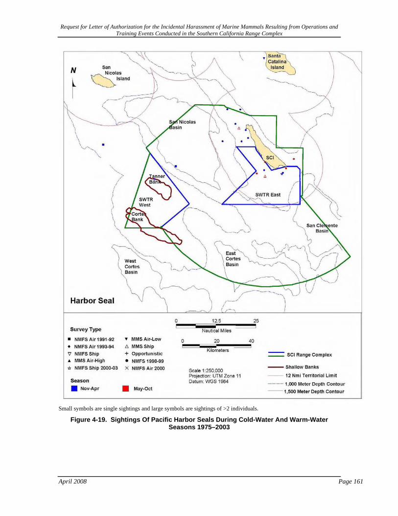
Request for Letter of Authorization for the Incidental Harassment of Marine Mammals Resulting from Operations and Training Events Conducted in the Southern California Range Complex
April 2008 Page 161
Small symbols are single sightings and large symbols are sightings of >2 individuals.
Figure 4-19. Sightings Of Pacific Harbor Seals During Cold-Water And Warm-Water Seasons 1975–2003

Request for Letter of Authorization for the Incidental Harassment of Marine Mammals Resulting from Operations and Training Events Conducted in the Southern California Range Complex
Page 162 April 2008
Small symbols are single sightings and large symbols are sightings of >2 individuals
Figure 4-20. Sightings of Northern Fur Seals During Cold-Water And Warm-Water Seasons 1975–2003

Request for Letter of Authorization for the Incidental Harassment of Marine Mammals Resulting from Operations and Training Events Conducted in the Southern California Range Complex
April 2008 Page 163
4.6 Cetacean Strandings and Threats Strandings can be a single animal or several to hundreds. An event where animals are found out of their normal habitat is considered a stranding even though animals do not necessarily end up beaching (such as the July 2004 Hanalei Mass Stranding Event; Southall et al. 2006). Several hypotheses have been given for the mass strandings which include the impact of shallow beach slopes on odontocete sonar, disease or parasites, geomagnetic anomalies that affect navigation, following a food source in close to shore, avoiding predators, social interactions that cause other cetaceans to come to the aid of stranded animals, and human actions. Generally, inshore species do not strand in large numbers but generally just as a single animal. This may be due to their familiarity with the coastal area whereas pelagic species that are unfamiliar with obstructions or sea bottom tend to strand more often in larger numbers (Woodings 1995). The Navy has studied several stranding events in detail that may have occurred in association with Navy sonar activities. To better understand the causal factors in stranding events that may be associated with Navy sonar activities, the main factors, including bathymetry (i.e., steep drop offs), narrow channels (less than 35 nm), environmental conditions (e.g., surface ducting), and multiple sonar ships (see Section on Stranding Events Associated with Navy Sonar) were compared between the different stranding events.
4.6.1 What is a Stranded Marine Mammal? When a live or dead marine mammal swims or floats onto shore and becomes “beached” or incapable of returning to sea, the event is termed a “stranding” (Geraci et al., 1999; Perrin and Geraci, 2002; Geraci and Lounsbury, 2005; NMFS, 2007). The legal definition for a stranding within the U.S. is that “a marine mammal is dead and is (i) on a beach or shore of the United States; or (ii) in waters under the jurisdiction of the United States (including any navigable waters); or (B) a marine mammal is alive and is (i) on a beach or shore of the United States and is unable to return to the water; (ii) on a beach or shore of the United States and, although able to return to the water, is in need of apparent medical attention; or (iii) in the waters under the jurisdiction of the United States (including any navigable waters), but is unable to return to its natural habitat under its own power or without assistance.” (16 United States Code [U.S.C.] 1421h).
The majority of animals that strand are dead or moribund (NMFS, 2007). For animals that strand alive, human intervention through medical aid and/or guidance seaward may be required for the animal to return to the sea. If unable to return to sea, rehabilitation at an appropriate facility may be determined as the best opportunity for animal survival. An event where animals are found out of their normal habitat is may be considered a stranding depending on circumstances even though animals do not necessarily end up beaching (Southhall, 2006).
Three general categories can be used to describe strandings: single, mass, and unusual mortality events. The most frequent type of stranding is a single stranding, which involves only one animal (or a mother/calf pair) (NMFS, 2007).
Mass stranding involves two or more marine mammals of the same species other than a mother/calf pair (Wilkinson, 1991), and may span one or more days and range over several miles (Simmonds and Lopez-Jurado, 1991; Frantzis, 1998; Walsh et al., 2001; Freitas, 2004). In North America, only a few species typically strand in large groups of 15 or more and include sperm whales, pilot whales, false killer whales, Atlantic white-sided dolphins, white-beaked dolphins, and rough-toothed dolphins (Odell 1987, Walsh et al. 2001). Some species, such as pilot whales,
Request for Letter of Authorization for the Incidental Harassment of Marine Mammals Resulting from Operations and Training Events Conducted in the Southern California Range Complex
Page 164 April 2008
false-killer whales, and melon-headed whales occasionally strand in groups of 50 to 150 or more (Geraci et al. 1999). All of these normally pelagic off-shore species are highly sociable and usually infrequently encountered in coastal waters. Species that commonly strand in smaller numbers include pygmy killer whales, common dolphins, bottlenose dolphins, Pacific white-sided dolphin Frasier’s dolphins, gray whale and humpback whale (West Coast only), harbor porpoise, Cuvier’s beaked whales, California sea lions, and harbor seals (Mazzuca et al. 1999, Norman et al. 2004, Geraci and Lounsbury 2005).
Unusual mortality events (UMEs) can be a series of single strandings or mass strandings, or unexpected mortalities (i.e., die-offs) that occur under unusual circumstances (Dierauf and Gulland, 2001; Harwood, 2002; Gulland, 2006; NMFS, 2007). These events may be interrelated: for instance, at-sea die-offs lead to increased stranding frequency over a short period of time, generally within one to two months (Table 4-3). As published by the NMFS, revised criteria for defining a UME include (71 FR 75234, 2006):
(1) A marked increase in the magnitude or a marked change in the nature of morbidity, mortality, or strandings when compared with prior records.
(2) A temporal change in morbidity, mortality, or strandings is occurring.
(3) A spatial change in morbidity, mortality, or strandings is occurring.
(4) The species, age, or sex composition of the affected animals is different than that of animals that are normally affected.
(5) Affected animals exhibit similar or unusual pathologic findings, behavior patterns, clinical signs, or general physical condition (e.g., blubber thickness).
(6) Potentially significant morbidity, mortality, or stranding is observed in species, stocks or populations that are particularly vulnerable (e.g., listed as depleted, threatened or endangered or declining). For example, stranding of three or four right whales may be cause for great concern whereas stranding of a similar number of fin whales may not.
(7) Morbidity is observed concurrent with or as part of an unexplained continual decline of a marine mammal population, stock, or species.
UMEs are usually unexpected, infrequent, and may involve a significant number of marine mammal mortalities. As discussed below, unusual environmental conditions are probably responsible for most UMEs and marine mammal die-offs (Vidal and Gallo-Reynoso, 1996; Geraci et al., 1999; Walsh et al., 2001; Gulland and Hall, 2005).
United States Stranding Response Organization Stranding events provide scientists and resource managers information not available from limited at-sea surveys, and may be the only way to learn key biological information about certain species such as distribution, seasonal occurrence, and health (Rankin, 1953; Moore et al., 2004; Geraci and Lounsbury, 2005). Necropsies are useful in attempting to determine a reason for the stranding, and are performed on stranded animals when the situation and resources allow.
In 1992, Congress amended the MMPA to establish the Marine Mammal Health and Stranding Response Act (MMHSRA) under authority of the Department of Commerce, National Marine Fisheries Service. The MMHSRP was created out of concern started in the 1980s for marine

Request for Letter of Authorization for the Incidental Harassment of Marine Mammals Resulting from Operations and Training Events Conducted in the Southern California Range Complex
April 2008 Page 165
mammal mortalities, to formalize the response process, and to focus efforts being initiated by numerous local stranding organizations and as a result of public concern.
Major elements of the MMHSRP include (NMFS, 2007):
• National Marine Mammal Stranding Network
• Marine Mammal UME Program
• National Marine Mammal Tissue Bank (NMMTB) and Quality Assurance Program
• Marine Mammal Health Biomonitoring, Research, and Development
• Marine Mammal Disentanglement Network
• John H. Prescott Marine Mammal Rescue Assistance Grant Program (a.k.a. the Prescott Grant Program)
• Information Management and Dissemination.
The United States has a well-organized network in coastal states to respond to marine mammal strandings. Overseen by the NMFS, the National Marine Mammal Stranding Network is comprised of smaller organizations manned by professionals and volunteers from nonprofit organizations, aquaria, universities, and state and local governments trained in stranding response, animal health, and diseased investigation. Currently, 141 organizations are authorized by NMFS to respond to marine mammal strandings (National Marine Fisheries Service, 2007o). Through a National Coordinator and six regional coordinators, NMFS authorizes and oversees stranding response activities and provides specialized training for the network.
NMFS Regions and Associated States and Territories
NMFS Northeast Region- ME, NH, MA, RI, CT, NY, NJ, PA, DE, MD, VA
NMFS Southeast Region- NC, SC, GA, FL, AL, MS, LA, TX, PR, VI
NMFS Southwest Region- CA
NMFS Northwest Region- OR, WA
NMFS Alaska Region- AK
NMFS Pacific Islands Region- HI, Guam, American Samoa, Commonwealth of the Northern Mariana Islands (CNMI)
Stranding reporting and response efforts over time have been inconsistent, although effort and data quality within the U.S. have been improving within the last 20 years (NMFS, 2007). Given the historical inconsistency in response and reporting, however, interpretation of long-term trends in marine mammal stranding is difficult (NMFS, 2007). During the past decade (1995 – 2004), approximately 40,000 (about 12,400 are cetaceans) stranded marine mammals have been reported by the regional stranding networks, averaging 3,600 strandings reported per year (Table 4-4; Figure 4-22) (NMFS, 2007). The highest number of strandings were reported between the years 1998 and 2003 (NMFS, 2007). Detailed regional stranding information including most commonly stranded species can be found in Zimmerman (1991), Geraci and Lounsbury (2005), and NMFS (2007).

Request for Letter of Authorization for the Incidental Harassment of Marine Mammals Resulting from Operations and Training Events Conducted in the Southern California Range Complex
Page 166 April 2008
4.6.2 Unusual Mortality Events (UMEs) Table 4-2 contains a list of documented UMEs within the U.S.
Table 4-2. Documented UMEs within the United States.
Year Composition Determination
1993 Harbor seals, Steller sea lions, and California sea lions on the central Washington coast Human Interaction
1993/1994 Bottlenose dolphins in the Gulf of Mexico Morbillivirus 1994 Common dolphins in California Cause not determined
1996 Right whales off Florida/Georgia coast Evidence of human interactions
1996 Manatees on the west coast of Florida Brevetoxin
1996 Bottlenose dolphins in Mississippi Cause not determined
1997 Harbor seals in California Unknown infectious respiratory disease
1997 Pinnipeds on the Pacific coast El Niño
1998 California sea lions in central California Harmful algal bloom; Domoic acid
1999 Harbor porpoises on the East Coast Determined not to meet criteria for UME because of multiplicity of causes
1999/2000 Bottlenose dolphins in the Panhandle of Florida
Harmful algal bloom is suspected; still under investigation
1999/2000 Gray whales from Alaska to Mexico Still under investigation
2004 Bottlenose dolphins along the Florida Panhandle
Uncertain, red tide is suspected
2005 Bottlenose dolphins, manatees, sea turtles, and seabirds in west central Florida Unknown
Source: NMFS 2007c
Table 4-3. Cetacean And Pinniped Stranding Count By NMFS Region 2001-2004.
NMFS Region # of Cetaceans # of Pinnipeds
Northeast 1,620 4,050 Southeast 2,830 45 Southwest 12,900 45 Northwest 188 1,430 Alaska 269 348 Pacific Islands 59 10 Four Year Total 17,866 5,928

Request for Letter of Authorization for the Incidental Harassment of Marine Mammals Resulting from Operations and Training Events Conducted in the Southern California Range Complex
April 2008 Page 167
Figure 4-21. United States Annual Cetacean And Pinniped Stranding From 1995-2004.
4.6.3 Threats to Marine Mammals and Potential Causes for Stranding Reports of marine mammal strandings can be traced back to ancient Greece (Walsh et al., 2001). Like any wildlife population, there are normal background mortality rates that influence marine mammal population dynamics, including starvation, predation, aging, reproductive success, and disease (Geraci et al. 1999; Carretta et al. 2007). Strandings in and of themselves may be reflective of this natural cycle or, more recently, may be the result of anthropogenic sources (i.e., human impacts). Current science suggests that multiple factors, both natural and man-made, may be acting alone or in combination to cause a marine mammal to strand (Geraci et al., 1999; Culik, 2002; Perrin and Geraci, 2002; Hoelzel, 2003; Geraci and Lounsbury, 2005; NRC, 2006). While post-stranding data collection and necropsies of dead animals are attempted in an effort to find a possible cause for the stranding, it is often difficult to pinpoint exactly one factor that can be blamed for any given stranding. An animal suffering from one ailment becomes susceptible to various other influences because of its weakened condition, making it difficult to determine a primary cause. In many stranding cases, scientists never learn the exact reason for the stranding.
0
1000
2000
3000
4000
5000
6000
1995 1996 1997 1998 1999 2000 2001 2002 2003 2004
Year
Num
ber o
f Stra
ndin
g (L
evel
A D
ata)
CetaceansPinniped
Source: NMFS 2007

Request for Letter of Authorization for the Incidental Harassment of Marine Mammals Resulting from Operations and Training Events Conducted in the Southern California Range Complex
Page 168 April 2008
Specific potential stranding causes can include both natural and human influenced (anthropogenic) causes listed below and described in the following sections:
Natural Stranding Causes
Disease
Natural toxins
Weather and climatic influences
Navigation errors
Social cohesion
Predation
Human Influenced (Anthropogenic) Stranding Causes
Fisheries interaction
Vessel strike
Pollution and ingestion
Noise
4.6.4 Natural Stranding Causes Significant natural causes of mortality, die-offs, and stranding discussed below include disease and parasitism; marine neurotoxins from algae; navigation errors that lead to inadvertent stranding; and climatic influences that impact the distribution and abundance of potential food resources (i.e., starvation). Other natural mortality not discussed in detail includes predation by other species such as sharks (Cockcroft et al., 1989; Heithaus, 2001), killer whales (Constantine et al. 1998; Guinet et al. 2000; Pitman et al. 2001), and some species of pinniped (Hiruki et al. 1999; Robinson et al. 1999).
Disease Like other mammals, marine mammals frequently suffer from a variety of diseases of viral, bacterial, parasites and fungal origin (Visser et al. 1991; Dunn et al. 2001; Harwood 2002). Gulland and Hall (2005) provide a more detailed summary of individual and population effects of marine mammal diseases.
Microparasites such as bacteria, viruses, and other microorganisms are commonly found in marine mammal habitats and usually pose little threat to a healthy animal (Geraci et al. 1999). For example, long-finned pilot whales that inhabit the waters off of the northeastern coast of the U.S. are carriers of the morbillivirus, yet have grown resistant to its usually lethal effects (Geraci et al. 1999). Since the 1980s, however, virus infections have been strongly associated with marine mammal die-offs (Domingo et al., 1992; Geraci and Lounsbury, 2005). Morbillivirus is the most significant marine mammal virus and suppresses a host’s immune system, increasing risk of secondary infection (Harwood 2002). A bottlenose dolphin UME in 1993 and 1994 was caused by infectious disease. Die-offs ranged from northwestern Florida to Texas, with an increased number of deaths as it spread (NMFS 2007c). A 2004 UME in Florida was also associated with dolphin morbillivirus (NMFS 2004). Influenza A was responsible for the first reported mass mortality in the U.S., occurring along the coast of New England in 1979-1980

Request for Letter of Authorization for the Incidental Harassment of Marine Mammals Resulting from Operations and Training Events Conducted in the Southern California Range Complex
April 2008 Page 169
(Geraci et al. 1999; Harwood 2002). Canine distemper virus (a type of morbillivirus) has been responsible for large scale pinniped mortalities and die-offs (Grachev et al. 1989; Kennedy et al., 2000; Gulland and Hall, 2005), while a bacteria, Leptospira pomona, is responsible for periodic die-offs in California sea lions about every four years (Gulland et al. 1996; Gulland and Hall 2005). It is difficult to determine whether microparasites commonly act as a primary pathogen, or whether they show up as a secondary infection in an already weakened animal (Geraci et al. 1999). Most marine mammal die-offs from infectious disease in the last 25 years, however, have had viruses associated with them (Simmonds and Mayer 1997; Geraci et al. 1999; Harwood 2002).
Macroparasites are usually large parasitic organisms and include lungworms, trematodes (parasitic flatworms), and protozoans (Geraci and St.Aubin 1987; Geraci et al. 1999). Marine mammals can carry many different types, and have shown a robust tolerance for sizeable infestation unless compromised by illness, injury, or starvation (Morimitsu et al. 1987; Dailey et al. 1991; Geraci et al., 1999). Nasitrema, a usually benign trematode found in the head sinuses of cetaceans (Geraci et al. 1999), can cause brain damage if it migrates (Ridgway and Dailey 1972). As a result, this worm is one of the few directly linked to stranding in the cetaceans (Dailey and Walker 1978; Geraci et al. 1999).
Non-infectious disease, such as congenital bone pathology of the vertebral column (osteomyelitis, spondylosis deformans, and ankylosing spondylitis [AS]), has been described in several species of cetacean (Paterson 1984; Alexander et al. 1989; Kompanje 1995; Sweeny et al. 2005). In humans, bone pathology such as AS, can impair mobility and increase vulnerability to further spinal trauma (Resnick and Niwayama 2002). Bone pathology has been found in cases of single strandings (Paterson 1984; Kompanje 1995), and also in cetaceans prone to mass stranding (Sweeny et al. 2005), possibly acting as a contributing or causal influence in both types of events.
Naturally Occurring Marine Neurotoxins Some single cell marine algae common in coastal waters, such as dinoflagellates and diatoms, produce toxic compounds that can accumulate (termed bioaccumulation) in the flesh and organs of fish and invertebrates (Geraci et al. 1999; Harwood 2002). Marine mammals become exposed to these compounds when they eat prey contaminated by these naturally produced toxins although exposure can also occur through inhalation and skin contact (Van Dolah 2005). Figure 4-23 shows U.S. animal mortalities from 1997-2006 resulting from toxins produced during harmful algal blooms.
In the Gulf of Mexico and mid- to southern Atlantic states, “red tides,” a form of harmful algal bloom, are created by a dinoflagellate (Karenia brevis). K. brevis is found throughout the Gulf of Mexico and sometimes along the Atlantic coast (Van Dolah 2005; NMFS 2007). It produces a neurotoxin known as brevetoxin. Brevetoxin has been associated with several marine mammal UMEs within this area (Geraci 1989; Van Dolah et al. 2003; NMFS 2004; Flewelling et al. 2005; Van Dolah 2005; NMFS 2007). On the U.S. west coast and in the northeast Atlantic, several species of diatoms produce a toxin called domoic acid which has also been linked to marine mammal strandings (Geraci et al. 1999; Van Dolah et al. 2003; Greig et al. 2005; Van Dolah 2005; Brodie et al. 2006; NMFS 2007; Bargu et al. 2008; Goldstein et al. 2008). Other algal toxins associated with marine mammal strandings include saxitoxins and ciguatoxins and are summarized by Van Dolah (2005).

Request for Letter of Authorization for the Incidental Harassment of Marine Mammals Resulting from Operations and Training Events Conducted in the Southern California Range Complex
Page 170 April 2008
Figure 4-22. Animal Mortalities From Harmful Algal Blooms Within The U.S. From 1997-2006.
Source: Woods Hole Oceanographic Institute (WHO) http://www.whoi.edu/redtide/HABdistribution/HABmap.html
Weather events and climate influences Severe storms, hurricanes, typhoons, and prolonged temperature extremes may lead to localized marine mammal strandings (Geraci et al., 1999; Walsh et al. 2001). Hurricanes may have been responsible for mass strandings of pygmy killer whales in the British Virgin Islands and Gervais’ beaked whales in North Carolina (Mignucci-Giannoni et al. 2000; Norman and Mead 2001). Storms in 1982-1983 along the California coast led to deaths of 2,000 northern elephant seal pups (Le Boeuf and Reiter 1991). Ice movement along southern Newfoundland has forced groups of blue whales and white-beaked dolphins ashore (Sergeant 1982). Seasonal oceanographic conditions in terms of weather, frontal systems, and local currents may also play a role in stranding (Walker et al. 2005).
The effect of large scale climatic changes to the world’s oceans and how these changes impact marine mammals and influence strandings is difficult to quantify given the broad spatial and temporal scales involved, and the cryptic movement patterns of marine mammals (Moore 2005; Learmonth et al. 2006). The most immediate, although indirect, effect is decreased prey availability during unusual conditions. This, in turn, results in increased search effort required by marine mammals (Crocker et al. 2006), potential starvation if not successful, and corresponding stranding due directly to starvation or succumbing to disease or predation while in a more weakened, stressed state (Selzer and Payne 1988; Geraci et al. 1999; Moore 2005; Learmonth et al. 2006; Weise et al. 2006).
Two recent papers examined potential influences of climate fluctuation on stranding events in southern Australia, including Tasmania, an area with a history of more than 20 mass stranding

Request for Letter of Authorization for the Incidental Harassment of Marine Mammals Resulting from Operations and Training Events Conducted in the Southern California Range Complex
April 2008 Page 171
since the 1920s (Evans et al. 2005; Bradshaw et al. 2006). These authors note that patterns in animal migration, survival, fecundity, population size, and strandings will revolve around the availability and distribution of food resources. In southern Australia, movement of nutrient-rich waters pushed closer to shore by periodic meridinal winds (occurring about every 12 – 14 years) may be responsible for bringing marine mammals closer to land, thus increasing the probability of stranding (Bradshaw et al. 2006). The papers conclude, however, that while an overarching model can be helpful for providing insight into the prediction of strandings, the particular reasons for each one are likely to be quite varied.
Navigation Error Geomagnetism- It has been hypothesized that, like some land animals, marine mammals may be able to orient to the Earth’s magnetic field as a navigational cue, and that areas of local magnetic anomalies may influence strandings (Bauer et al. 1985; Klinowska 1985; Kirschvink et al. 1986; Klinowska, 1986; Walker et al. 1992; Wartzok and Ketten 1999). In a plot of live stranding positions in Great Britain with magnetic field maps, Klinowska (1985; 1986) observed an association between live stranding positions and magnetic field levels. In all cases, live strandings occurred at locations where magnetic minima, or lows in the magnetic fields, intersect the coastline. Kirschvink et al. (1986) plotted stranding locations on a map of magnetic data for the east coast of the U.S., and were able to develop associations between stranding sites and locations where magnetic minima intersected the coast. The authors concluded that there were highly significant tendencies for cetaceans to beach themselves near these magnetic minima and coastal intersections. The results supported the hypothesis that cetaceans may have a magnetic sensory system similar to other migratory animals, and that marine magnetic topography and patterns may influence long-distance movements (Kirschvink et al. 1986). Walker et al. (1992) examined fin whale swim patterns off the northeastern U.S. continental shelf, and reported that migrating animals aligned with lows in the geometric gradient or intensity. While a similar pattern between magnetic features and marine mammal strandings at New Zealand stranding sites was not seen (Brabyn and Frew, 1994), mass strandings in Hawaii typically were found to occur within a narrow range of magnetic anomalies (Mazzuca et al. 1999).
Echolocation Disruption in Shallow Water- Some researchers believe stranding may result from reductions in the effectiveness of echolocation within shallow water, especially with the pelagic species of odontocetes who may be less familiar with coastline (Dudok van Heel 1966; Chambers and James 2005). For an odontocete, echoes from echolocation signals contain important information on the location and identity of underwater objects and the shoreline. The authors postulate that the gradual slope of a beach may present difficulties to the navigational systems of some cetaceans, since it is common for live strandings to occur along beaches with shallow, sandy gradients (Brabyn and McLean 1992; Mazzuca et al. 1999; Maldini et al. 2005; Walker et al. 2005). A contributing factor to echolocation interference in turbulent, shallow water is the presence of microbubbles from the interaction of wind, breaking waves, and currents. Additionally, ocean water near the shoreline can have an increased turbidity (e.g., floating sand or silt, particulate plant matter, etc.) due to the run-off of fresh water into the ocean, either from rainfall or from freshwater outflows (e.g., rivers and creeks). Collectively, these factors can reduce and scatter the sound energy within echolocation signals and reduce the perceptibility of returning echoes of interest.

Request for Letter of Authorization for the Incidental Harassment of Marine Mammals Resulting from Operations and Training Events Conducted in the Southern California Range Complex
Page 172 April 2008
Social cohesion Many pelagic species such as sperm whale, pilot whales, melon-head whales, and false killer whales, and some dolphins occur in large groups with strong social bonds between individuals. When one or more animals strand due to any number of causative events, then the entire pod may follow suit out of social cohesion (Geraci et al. 1999; Conner 2000; Perrin and Geraci 2002; NMFS 2007).
4.6.5 Anthropogenic Stranding Causes and Potential Risks With the exception of historic whaling in the 19th and early part of the 20th century, over the past few decades there has been an increase in marine mammal mortalities associated with a variety of human activities (Geraci et al. 1999; NMFS 2007). These include fisheries interactions (bycatch and directed catch), pollution (marine debris, toxic compounds), habitat modification (degradation, prey reduction), direct trauma (vessel strikes, gunshots), and noise. Figure 4-24 shows potential worldwide risk to small toothed cetaceans by source.
Fisheries Interaction: By-Catch, Directed Catch, and Entanglement The incidental catch of marine mammals in commercial fisheries is a significant threat to the survival and recovery of many populations of marine mammals (Geraci et al., 1999; Baird 2002; Culik 2002; Carretta et al. 2004; Geraci and Lounsbury 2005; NMFS 2007). Interactions with fisheries and entanglement in discarded or lost gear continue to be a major factor in marine mammal deaths worldwide (Geraci et al. 1999; Nieri et al. 1999; Geraci and Lounsbury 2005; Read et al. 2006; Zeeberg et al. 2006). For instance, baleen whales and pinnipeds have been found entangled in nets, ropes, monofilament line, and other fishing gear that has been discarded out at sea (Geraci et al. 1999; Campagna et al. 2007).
Bycatch- Bycatch is the catching of non-target species within a given fishing operation and can include non-commercially used invertebrates, fish, sea turtles, birds, and marine mammals (NRC 2006). Read et al. (2006) attempted to estimate the magnitude of marine mammal bycatch in U.S. and global fisheries. Data on marine mammal bycatch within the United States was obtained from fisheries observer programs, reports of entangled stranded animals, and fishery logbooks, and was then extrapolated to estimate global bycatch by using the ratio of U.S. fishing vessels to the total number of vessels within the world’s fleet (Read et al. 2006). Within U.S. fisheries, between 1990 and 1999 the mean annual bycatch of marine mammals was 6,215 animals, with a standard error of +/- 448 (Read et al. 2006).
Eight-four percent of cetacean bycatch occurred in gill-net fisheries, with dolphins and porpoises constituting most of the cetacean bycatch (Read et al. 2006). Over the decade there was a 40 percent decline in marine mammal bycatch, which was significantly lower from 1995-1999 than it was from 1990-1994 (Read et al. 2006). Read et al. (2006) suggests that this is primarily due to effective conservation measures that were implemented during this time period.
Read et al. (2006) then extrapolated this data for the same time period and calculated an annual estimate of 653,365 of marine mammals globally, with most of the world’s bycatch occurring in gill-net fisheries. With global marine mammal bycatch likely to be in the hundreds of thousands every year, bycatch in fisheries will be the single greatest threat to many marine mammal populations around the world (Read et al. 2006).

Request for Letter of Authorization for the Incidental Harassment of Marine Mammals Resulting from Operations and Training Events Conducted in the Southern California Range Complex
April 2008 Page 173
26.5%
24.9%
21.2%
9.0%
6.9%5.8%
4.8%
1.1%
0%
5%
10%
15%
20%
25%
30%
Fisheries-Bycatch
Fisheries-Directed
Catch
Pollution HabitatDegradation
Unknown PreyOverfishing
Fisheries-Culling
Noise
Category of threat
Perc
ent o
f 71
smal
l cet
acea
n sp
ecie
s th
reat
ened
(Source: Culik 2002)
Figure 4-23. Human Threats to World Wide Small Cetacean Populations
Entanglement- Entanglement in active fishing gear is a major cause of death or severe injury among the endangered whales in the action area. Entangled marine mammals may die as a result of drowning, escape with pieces of gear still attached to their bodies, or manage to be set free either of their own accord or by fishermen. Many large whales carry off gear after becoming entangled (Read et al. 2006). Many times when a marine mammal swims off with gear attached, the end result can be fatal. The gear may be become too cumbersome for the animal, or it can be wrapped around a crucial body part and tighten over time. Stranded marine mammals frequently exhibit signs of previous fishery interaction, such as scarring or gear attached to their bodies, and the cause of death for many stranded marine mammals is often attributed to such interactions (Baird and Gorgone 2005). Marine mammals that die or are injured in fisheries activities may not wash ashore, therefore stranding data may underestimate fishery-related mortalities and serious injuries (NMFS 2005a).

Request for Letter of Authorization for the Incidental Harassment of Marine Mammals Resulting from Operations and Training Events Conducted in the Southern California Range Complex
Page 174 April 2008
From 1993 through 2003, 1,105 harbor porpoises were reported stranded from Maine to North Carolina, many of which had cuts and body damage suggestive of net entanglement (NMFS 2005e). In 1999 it was possible to determine that the cause of death for 38 of the stranded porpoises was from fishery interactions, with one additional animal having been mutilated (right flipper and fluke cut off) (NMFS 2005e). In 2000, one stranded porpoise was found with monofilament line wrapped around its body (NMFS 2005e). In 2003, nine stranded harbor porpoises were attributed to fishery interactions, with an additional three mutilated animals (NMFS 2005e). An estimated 78 baleen whales were killed annually in the offshore southern California/Oregon drift gillnet fishery during the 1980s (Heyning and Lewis 1990). From 1998-2005, based on observer records, five fin whales (CA/OR/WA stock), 12 humpback whales (ENP stock), and six sperm whales (CA/OR/WA stock) were either seriously injured or killed in fisheries off the mainland west coast of the U.S. (California Marine Mammal Stranding Network Database 2006).
Ship Strike Vessel strikes to marine mammals are another cause of mortality and stranding (Laist et al. 2001; Geraci and Lounsbury 2005; de Stephanis and Urquiola, 2006). An animal at the surface could be struck directly by a vessel, a surfacing animal could hit the bottom of a vessel, or an animal just below the surface could be cut by a vessel’s propeller. The severity of injuries typically depends on the size and speed of the vessel (Knowlton and Kraus 2001; Laist et al. 2001; Vanderlaan and Taggart 2007).
An examination of all known ship strikes from all shipping sources (civilian and military) indicates vessel speed is a principal factor in whether a vessel strike results in death (Knowlton and Kraus 2001; Laist et al. 2001, Jensen and Silber 2003; Vanderlaan and Taggart 2007). In assessing records in which vessel speed was known, Laist et al. (2001) found a direct relationship between the occurrence of a whale strike and the speed of the vessel involved in the collision. The authors concluded that most deaths occurred when a vessel was traveling in excess of 13 knots although most vessels do travel greater than 15 kts. Jensen and Silber (2003) detailed 292 records of known or probable ship strikes of all large whale species from 1975 to 2002. Of these, vessel speed at the time of collision was reported for 58 cases. Of these cases, 39 (or 67%) resulted in serious injury or death (19 or 33% resulted in serious injury as determined by blood in the water, propeller gashes or severed tailstock, and fractured skull, jaw, vertebrae, hemorrhaging, massive bruising or other injuries noted during necropsy and 20 or 35% resulted in death). Operating speeds of vessels that struck various species of large whales ranged from 2 to 51 knots. The majority (79%) of these strikes occurred at speeds of 13 knots or greater. The average speed that resulted in serious injury or death was 18.6 knots. Pace and Silber (2005) found that the probability of death or serious injury increased rapidly with increasing vessel speed. Specifically, the predicted probability of serious injury or death increased from 45 percent to 75 % as vessel speed increased from 10 to 14 knots, and exceeded 90% at 17 knots. Higher speeds during collisions result in greater force of impact, but higher speeds also appear to increase the chance of severe injuries or death by pulling whales toward the vessel. Computer simulation modeling showed that hydrodynamic forces pulling whales toward the vessel hull increase with increasing speed (Clyne 1999, Knowlton et al. 1995).
The growth in civilian commercial ports and associated commercial vessel traffic is a result in the globalization of trade. The Final Report of the NOAA International Symposium on “Shipping Noise and Marine Mammals: A Forum for Science, Management, and Technology”

Request for Letter of Authorization for the Incidental Harassment of Marine Mammals Resulting from Operations and Training Events Conducted in the Southern California Range Complex
April 2008 Page 175
stated that the worldwide commercial fleet has grown from approximately 30,000 vessels in 1950 to over 85,000 vessels in 1998 (NRC, 2003; Southall, 2005). Between 1950 and 1998, the U.S. flagged fleet declined from approximately 25,000 to less than 15,000 and currently represents only a small portion of the world fleet. From 1985 to 1999, world seaborne trade doubled to 5 billion tons and currently includes 90 percent of the total world trade, with container shipping movements representing the largest volume of seaborne trade. It is unknown how international shipping volumes and densities will continue to grow. However, current statistics support the prediction that the international shipping fleet will continue to grow at the current rate or at greater rates in the future. Shipping densities in specific areas and trends in routing and vessel design are as, or more, significant than the total number of vessels. Densities along existing coastal routes are expected to increase both domestically and internationally. New routes are also expected to develop as new ports are opened and existing ports are expanded. Vessel propulsion systems are also advancing toward faster ships operating in higher sea states for lower operating costs; and container ships are expected to become larger along certain routes (Southall 2005).
While there are reports and statistics of whales struck by vessels in U.S. waters, the magnitude of the risks of commercial ship traffic poses to marine mammal populations is difficult to quantify or estimate. In addition, there is limited information on vessel strike interactions between ships and marine mammals outside of U.S. waters (de Stephanis and Urquiola 2006). Laist et al. (2001) concluded that ship collisions may have a negligible effect on most marine mammal populations in general, except for regional based small populations where the significance of low numbers of collisions would be greater given smaller populations or populations segments.
U.S. Navy vessel traffic is a small fraction of the overall U.S. commercial and fishing vessel traffic. While U.S. Navy vessel movements may contribute to the ship strike threat, given the lookout and mitigation measures adopted by the U.S. Navy, probability of vessel strikes is greatly reduced. Furthermore, actions to avoid close interaction of U.S. Navy ships and marine mammals and sea turtles, such as maneuvering to keep away from any observed marine mammal and sea turtle are part of existing at-sea protocols and standard operating procedures. Navy ships have up to three or more dedicated and trained lookouts as well as two to three bridge watchstanders during at-sea movements who would be searching for any whales, sea turtles, or other obstacles on the water surface. Such lookouts are expected to further reduce the chances of a collision.
Commercial and Private Marine Mammal Viewing In addition to vessel operations, private and commercial vessels engaged in marine mammal watching also have the potential to impact marine mammals in Southern California. NMFS has promulgated regulations at 50 CFR 224.103, which provide specific prohibitions regarding wildlife viewing activities. In addition, NMFS launched an education and outreach campaign to provide commercial operators and the general public with responsible marine mammal viewing guidelines. In January 2002, NMFS also published an official policy on human interactions with wild marine mammals which states that: “NOAA Fisheries cannot support, condone, approve or authorize activities that involve closely approaching, interacting or attempting to interact with whales, dolphins, porpoises, seals, or sea lions in the wild. This includes attempting to swim, pet, touch or elicit a reaction from the animals.”

Request for Letter of Authorization for the Incidental Harassment of Marine Mammals Resulting from Operations and Training Events Conducted in the Southern California Range Complex
Page 176 April 2008
Although considered by many to be a non-consumptive use of marine mammals with economic, recreational, educational, and scientific benefits, marine mammal watching is not without potential negative impacts. One concern is that animals become more vulnerable to vessel strikes once they habituate to vessel traffic (Swingle et al. 1993; Wiley et al. 1995). Another concern is that preferred habitats may become abandoned if disturbance levels are too high. A whale’s behavioral response to whale watching vessels depends on the distance of the vessel from the whale, vessel speed, vessel direction, vessel noise, and the number of vessels (Amaral and Carlson 2005; Au and Green 2000; Cockeron 1995; Erbe 2002; Magalhaes et al. 2002; Richter et al. 2003; Schedat et al. 2004; Simmonds 2005; Watkins 1986; Williams et al. 2002). The whale’s responses changed with these different variables and, in some circumstances, the whales did not respond to the vessels, but in other circumstances, whales changed their vocalizations surface time, swimming speed, swimming angle or direction, respiration rates, dive times, feeding behavior, and social interactions. In addition to the information on whale watching, there is also direct evidence of pinniped haul out site (Pacific harbor seals) abandonment because of human disturbance at Strawberry Spit in San Francisco Bay (Allen 1991).
Ingestion of Plastic Objects and Other Marine Debris And Toxic Pollution Exposure
For many marine mammals, debris in the marine environment is a great hazard and can be harmful to wildlife. Not only is debris a hazard because of possible entanglement, animals may mistake plastics and other debris for food (NMFS, 2007g). There are certain species of cetaceans, along with Florida manatees, that are more likely to eat trash, especially plastics, which is usually fatal for the animal (Geraci et al. 1999).
Between 1990 through October 1998, 215 pygmy sperm whales stranded along the U.S. Atlantic coast from New York through the Florida Keys (NMFS 2005a). Remains of plastic bags and other debris were found in the stomachs of 13 of these animals (NMFS 2005a). During the same time period, 46 dwarf sperm whale strandings occurred along the U.S. Atlantic coastline between Massachusetts and the Florida Keys (NMFS 2005d). In 1987 a pair of latex examination gloves was retrieved from the stomach of a stranded dwarf sperm whale (NMFS 2005d). 125 pygmy sperm whales were reported stranded from 1999 – 2003 between Maine and Puerto Rico; in one pygmy sperm whale found stranded in 2002, red plastic debris was found in the stomach along with squid beaks (NMFS 2005a).
Sperm whales have been known to ingest plastic debris, such as plastic bags (Evans et al. 2003; Whitehead 2003). While this has led to mortality, the scale to which this is affecting sperm whale populations is unknown, but Whitehead (2003) suspects it is not substantial at this time.
High concentrations of potentially toxic substances within marine mammals along with an increase in new diseases have been documented in recent years. Scientists have begun to consider the possibility of a link between pollutants and marine mammal mortality events. NMFS takes part in a marine mammal bio-monitoring program not only to help assess the health and contaminant loads of marine mammals, but also to assist in determining anthropogenic impacts on marine mammals, marine food chains and marine ecosystem health. Using strandings and bycatch animals, the program provides tissue/serum archiving, samples for analyses, disease monitoring and reporting, and additional response during disease investigations (NMFS 2007).

Request for Letter of Authorization for the Incidental Harassment of Marine Mammals Resulting from Operations and Training Events Conducted in the Southern California Range Complex
April 2008 Page 177
The impacts of these activities are difficult to measure. However, some researchers have correlated contaminant exposure to possible adverse health effects in marine mammals. Contaminants such as organochlorines do not tend to accumulate in significant amounts in invertebrates, but do accumulate in fish and fish-eating animals. Thus, contaminant levels in planktivorous mysticetes have been reported to be one to two orders of magnitude lower compared to piscivorous odontocetes (Borell 1993; O’Shea and Brownell 1994; O’Hara and Rice 1996; O’Hara et al. 1999).
The manmade chemical PCB (polychlorinated biphenyl), and the pesticide DDT (dichlorodiphyenyltrichloroethane), are both considered persistent organic pollutants that are currently banned in the United States for their harmful effects in wildlife and humans (NMFS, 2007c). Despite having been banned for decades, the levels of these compounds are still high in marine mammal tissue samples taken along U.S. coasts (NMFS, 2007c). Both compounds are long-lasting, reside in marine mammal fat tissues (especially in the blubber), and can be toxic causing effects such as reproductive impairment and immunosuppression (NMFS, 2007c).
Both long-finned and short-finned pilot whales have a tendency to mass strand throughout their range. Short-finned pilot whales have been reported as stranded as far north as Rhode Island, and long-finned pilot whales as far south as South Carolina (NMFS 2005b). For U.S. east coast stranding records, both species are lumped together and there is rarely a distinction between the two because of uncertainty in species identification (NMFS 2005b). Since 1980 within the Northeast region alone, between 2 and 120 pilot whales have stranded annually either individually or in groups (NMFS 2005b). Between 1999 and 2003 from Maine to Florida, 126 pilot whales were reported to be stranded, including a mass stranding of 11 animals in 2000 and another mass stranding of 57 animals in 2002, both along the Massachusetts coast (NMFS 2005b).
It is unclear how much of a role human activities play in these pilot whale strandings, and toxic poisoning may be a potential human-caused source of mortality for pilot whales (NMFS 2005b). Moderate levels of PCBs and chlorinated pesticides (such as DDT, DDE, and dieldrin) have been found in pilot whale blubber (NMFS 2005b). Bioaccumulation levels have been found to be more similar in whales from the same stranding event than from animals of the same age or sex (NMFS 2005b). Numerous studies have measured high levels of toxic metals (mercury, lead, and cadmium), selenium, and PCBs in pilot whales in the Faroe Islands (NMFS 2005b). Population effects resulting from such high contamination levels are currently unknown (NMFS 2005b).
Habitat contamination and degradation may also play a role in marine mammal mortality and strandings. Some events caused by man have direct and obvious effects on marine mammals, such as oil spills (Geraci et al. 1999). But in most cases, effects of contamination will more than likely be indirect in nature, such as effects on prey species availability, or by increasing disease susceptibility (Geraci et al. 1999).
U.S. Navy vessel operation between ports and exercise locations has the potential for release of small amounts of pollutant discharges into the water column. U.S. Navy vessels are not a typical source, however, of either pathogens or other contaminants with bioaccumulation potential such as pesticides and PCBs. Furthermore, any vessel discharges such as bilgewater and deck runoff associated with the vessels would be in accordance with international and U.S. requirements for

Request for Letter of Authorization for the Incidental Harassment of Marine Mammals Resulting from Operations and Training Events Conducted in the Southern California Range Complex
Page 178 April 2008
eliminating or minimizing discharges of oil, garbage, and other substances, and not likely to contribute significant changes to ocean water quality.
For many marine mammals, debris in the marine environment is a great hazard and can be harmful to wildlife. Not only is debris a hazard because of possible entanglement, animals may mistake plastics and other debris for food (NMFS 2007g). There are certain species of cetaceans, along with Florida manatees, that are more likely to eat trash, especially plastics, which is usually fatal for the animal (Geraci et al. 1999).
Between 1990 through October 1998, 215 pygmy sperm whales stranded along the U.S. Atlantic coast from New York through the Florida Keys (NMFS 2005a). Remains of plastic bags and other debris were found in the stomachs of 13 of these animals (NMFS 2005a). During the same time period, 46 dwarf sperm whale strandings occurred along the U.S. Atlantic coastline between Massachusetts and the Florida Keys (NMFS 2005d). In 1987 a pair of latex examination gloves was retrieved from the stomach of a stranded dwarf sperm whale (NMFS 2005d). 125 pygmy sperm whales were reported stranded from 1999 – 2003 between Maine and Puerto Rico; in one pygmy sperm whale found stranded in 2002, red plastic debris was found in the stomach along with squid beaks (NMFS 2005a).
Sperm whales have been known to ingest plastic debris, such as plastic bags (Evans et al. 2003; Whitehead 2003). While this has led to mortality, the scale to which this is affecting sperm whale populations is unknown, but Whitehead (2003) suspects it is not substantial at this time.
High concentrations of potentially toxic substances within marine mammals along with an increase in new diseases have been documented in recent years. Scientists have begun to consider the possibility of a link between pollutants and marine mammal mortality events. NMFS takes part in a marine mammal bio-monitoring program not only to help assess the health and contaminant loads of marine mammals, but also to assist in determining anthropogenic impacts on marine mammals, marine food chains and marine ecosystem health. Using strandings and bycatch animals, the program provides tissue/serum archiving, samples for analyses, disease monitoring and reporting, and additional response during disease investigations (NMFS 2007).
The impacts of these activities are difficult to measure. However, some researchers have correlated contaminant exposure to possible adverse health effects in marine mammals. Contaminants such as organochlorines do not tend to accumulate in significant amounts in invertebrates, but do accumulate in fish and fish-eating animals. Thus, contaminant levels in planktivorous mysticetes have been reported to be one to two orders of magnitude lower compared to piscivorous odontocetes (Borell 1993; O’Shea and Brownell 1994; O’Hara and Rice 1996; O’Hara et al. 1999).
The manmade chemical PCB (polychlorinated biphenyl), and the pesticide DDT (dichlorodiphyenyltrichloroethane), are both considered persistent organic pollutants that are currently banned in the United States for their harmful effects in wildlife and humans (NMFS 2007c). Despite having been banned for decades, the levels of these compounds are still high in marine mammal tissue samples taken along U.S. coasts (NMFS 2007c). Both compounds are long-lasting, reside in marine mammal fat tissues (especially in the blubber), and can be toxic causing effects such as reproductive impairment and immunosuppression (NMFS 2007c).

Request for Letter of Authorization for the Incidental Harassment of Marine Mammals Resulting from Operations and Training Events Conducted in the Southern California Range Complex
April 2008 Page 179
Both long-finned and short-finned pilot whales have a tendency to mass strand throughout their range. Short-finned pilot whales have been reported as stranded as far north as Rhode Island, and long-finned pilot whales as far south as South Carolina (NMFS 2005b). For U.S. east coast stranding records, both species are lumped together and there is rarely a distinction between the two because of uncertainty in species identification (NMFS, 2005b). Since 1980 within the Northeast region alone, between 2 and 120 pilot whales have stranded annually either individually or in groups (NMFS, 2005b). Between 1999 and 2003 from Maine to Florida, 126 pilot whales were reported to be stranded, including a mass stranding of 11 animals in 2000 and another mass stranding of 57 animals in 2002, both along the Massachusetts coast (NMFS, 2005b).
It is unclear how much of a role human activities play in these pilot whale strandings, and toxic poisoning may be a potential human-caused source of mortality for pilot whales (NMFS 2005b). Moderate levels of PCBs and chlorinated pesticides (such as DDT, DDE, and dieldrin) have been found in pilot whale blubber (NMFS 2005b). Bioaccumulation levels have been found to be more similar in whales from the same stranding event than from animals of the same age or sex (NMFS 2005b). Numerous studies have measured high levels of toxic metals (mercury, lead, and cadmium), selenium, and PCBs in pilot whales in the Faroe Islands (NMFS 2005b). Population effects resulting from such high contamination levels are currently unknown (NMFS 2005b).
Habitat contamination and degradation may also play a role in marine mammal mortality and strandings. Some events caused by man have direct and obvious effects on marine mammals, such as oil spills (Geraci et al. 1999). But in most cases, effects of contamination will more than likely be indirect in nature, such as effects on prey species availability, or by increasing disease susceptibility (Geraci et al. 1999).
U.S. Navy vessel operation between ports and exercise locations has the potential for release of small amounts of pollutant discharges into the water column. U.S. Navy vessels are not a typical source, however, of either pathogens or other contaminants with bioaccumulation potential such as pesticides and PCBs. Furthermore, any vessel discharges such as bilgewater and deck runoff associated with the vessels would be in accordance with international and U.S. requirements for eliminating or minimizing discharges of oil, garbage, and other substances, and not likely to contribute significant changes to ocean water quality.
Deep Water Ambient Noise Urick (1983) provided a discussion of the ambient noise spectrum expected in the deep ocean. Shipping, seismic activity, and weather, are the primary causes of deep-water ambient noise. The ambient noise frequency spectrum can be predicted fairly accurately for most deep-water areas based primarily on known shipping traffic density and wind state (wind speed, Beaufort wind force, or sea state) (Urick 1983). For example, for frequencies between 100 and 500 Hz, Urick (1983) estimated the average deep water ambient noise spectra to be 73 to 80 dB for areas of heavy shipping traffic and high sea states, and 46 to 58 dB for light shipping and calm seas.
Shallow Water Ambient Noise In contrast to deep water, ambient noise levels in shallow waters (i.e., coastal areas, bays, harbors, etc.) are subject to wide variations in level and frequency depending on time and location. The primary sources of noise include distant shipping and industrial activities, wind and waves, marine animals (Urick 1983). At any give time and place, the ambient noise is a

Request for Letter of Authorization for the Incidental Harassment of Marine Mammals Resulting from Operations and Training Events Conducted in the Southern California Range Complex
Page 180 April 2008
mixture of all of these noise variables. In addition, sound propagation is also affected by the variable shallow water conditions, including the depth, bottom slope, and type of bottom. Where the bottom is reflective, the sounds levels tend to be higher, then when the bottom is absorptive.
Noise from Aircraft and Vessel Movement Surface shipping is the most widespread source of anthropogenic, low frequency (0 to 1,000 Hz) noise in the oceans and may contribute to over 75% of all human sound in the sea (Simmonds and Hutchinson 1996, ICES 2005b). The Navy estimated that the 60,000 vessels of the world’s merchant fleet, annually emit low frequency sound into the world’s oceans for the equivalent of 21.9 million days, assuming that 80 percent of the merchant ships are at sea at any one time (U.S. Navy 2001). Ross (1976) has estimated that between 1950 and 1975, shipping had caused a rise in ambient noise levels of 10 dB and predicted this would increase by another 5 dB by the beginning of the 21st century. The National Resource Council (1997) estimated that the background ocean noise level at 100 Hz has been increasing by about 1.5 dB per decade since the advent of propeller-driven ships. Michel et al. (2001) suggested an association between long-term exposure to low frequency sounds from shipping and an increased incidence of marine mammal mortalities caused by collisions with ships.
Airborne sound from a low-flying helicopter or airplane may be heard by marine mammals and turtles while at the surface or underwater. Due to the transient nature of sounds from aircraft involved in at-sea operations, such sounds would not likely cause physical effects but have the potential to affect behaviors. Responses by mammals and turtles could include hasty dives or turns, or decreased foraging (Soto et al., 2006). Whales may also slap the water with flukes or flippers, swim away from the aircraft track.
Sound emitted from large vessels, particularly in the course of transit, is the principal source of noise in the ocean today, primarily due to the properties of sound emitted by civilian cargo vessels (Richardson et al., 1995; Arveson and Vendittis, 2000). Ship propulsion and electricity generation engines, engine gearing, compressors, bilge and ballast pumps, as well as hydrodynamic flow surrounding a ship’s hull and any hull protrusions contribute to a large vessels’ noise emission into the marine environment. Prop-driven vessels also generate noise through cavitation, which accounts much of the noise emitted by a large vessel depending on its travel speed. Military vessels underway or involved in naval operations or exercises, also introduce anthropogenic noise into the marine environment. Noise emitted by large vessels can be characterized as low-frequency, continuous, and tonal. The sound pressure levels at the vessel will vary according to speed, burden, capacity and length (Richardson et al. 1995; Arveson and Vendittis, 2000). Vessels ranging from 135 to 337 meters generate peak source sound levels from 169- 200 dB between 8 Hz and 430 Hz, although Arveson and Vendittis (2000) documented components of higher frequencies (10-30 kHz) as a function of newer merchant ship engines and faster transit speeds. Any masking of environmental sounds or conspecific sounds is expected to be temporary, as noise dissipates with a vessel transit through an area.
Whales have variable responses to vessel presence or approaches, ranging from apparent tolerance to diving away from a vessel. Unfortunately, it is not always possible to determine whether the whales are responding to the vessel itself or the noise generated by the engine and cavitation around the propeller. Apart from some disruption of behavior, an animal may be unable to hear other sounds in the environment due to masking by the noise from the vessel.

Request for Letter of Authorization for the Incidental Harassment of Marine Mammals Resulting from Operations and Training Events Conducted in the Southern California Range Complex
April 2008 Page 181
Any masking of environmental sounds or conspecific sounds is expected to be temporary, as noise dissipates with a vessel transit through an area.
Vessel noise primarily raises concerns for masking of environmental and conspecific cues. However, exposure to vessel noise of sufficient intensity and/or duration can also result in temporary or permanent loss of sensitivity at a given frequency range, referred to as temporary or permanent threshold shifts (TTS or PTS). Threshold shifts are assumed to be possible in marine mammal species as a result of prolonged exposure to large vessel traffic noise due to its intensity, broad geographic range of effectiveness, and constancy.
Collectively, significant cumulative exposure to individuals, groups, or populations can occur if they exhibit site fidelity to a particular area; for example, whales that seasonally travel to a regular area to forage or breed may be more vulnerable to noise from large vessels compared to transiting whales. Any permanent threshold shift in a marine animal’s hearing capability, especially at particular frequencies for which it can normally hear best, can impair its ability to perceive threats, including ships. Whales have variable responses to vessel presence or approaches, ranging from apparent tolerance to diving away from a vessel. It is not possible to determine whether the whales are responding to the vessel itself or the noise generated by the engine and cavitation around the propeller. Apart from some disruption of behavior, an animal may be unable to hear other sounds in the environment due to masking by the noise from the vessel.
Most observations of behavioral responses of marine mammals to human generated sounds have been limited to short-term behavioral responses, which included the cessation of feeding, resting, or social interactions. Nowacek et al. (2007) provide a detailed summary of cetacean response to underwater noise.
Given the sound propagation of low frequency sounds, a large vessel in this sound range can be heard 139-463 kilometers away (Ross 1976 in Polefka 2004). U.S. Navy vessels, however, have incorporated significant underwater ship quieting technology to reduce their acoustic signature (as compared to a similarly-sized vessel) in order to reduce their vulnerability to detection by enemy passive acoustics (Southall, 2005). Therefore, the potential for TTS or PTS from U.S. Navy vessel and aircraft movement is extremely low given that the exercises and training events are transitory in time, with vessels moving over large area of the ocean. A marine mammal or sea turtle is unlikely to be exposed long enough at high levels for TTS or PTS to occur. Any masking of environmental sounds or conspecific sounds is expected to be temporary, as noise dissipates with a U.S. Navy vessel transiting through an area. If behavioral disruptions result from the presence of aircraft or vessels, it is expected to be temporary. Animals are expected to resume their migration, feeding, or other behaviors without any threat to their survival or reproduction. However, if an animal is aware of a vessel and dives or swims away, it may successfully avoid being struck.
Stranding Events Associated with Navy Sonar There are two classes of sonars employed by the U.S. Navy: active sonars and passive sonars. Most active military sonars operate in a limited number of areas, and are most likely not a significant contributor to a comprehensive global ocean noise budget (ICES 2005b).
The effects of mid-frequency active naval sonar on marine wildlife have not been studied as extensively as the effects of air-guns used in seismic surveys (Madsen et al. 2006; Stone and

Request for Letter of Authorization for the Incidental Harassment of Marine Mammals Resulting from Operations and Training Events Conducted in the Southern California Range Complex
Page 182 April 2008
Tasker 2006; Wilson et al. 2006; Palka and Johnson 2007; Parente et al. 2007). Maybaum (1989, 1993) observed changes in behavior of humpbacks during playback tapes of the M-1002 system (using 203 dB re 1 µPa-m for study); specifically, a decrease in respiration, submergence, and aerial behavior rates; and an increase in speed of travel and track linearity. Direct comparison of Maybaum’s results, however, with U.S Navy mid-frequency active sonar are difficult to make. Maybaum’s signal source, the commercial M-1002, is not similar to how naval mid-frequency sonar operates. In addition, behavioral responses were observed during playbacks of a control tape, (i.e., a tape with no sound signal) so interpretation of Maybaum’s results are inconclusive.
Research by Nowacek, et al. (2004) on North Atlantic right whales using a whale alerting signal designed to alert whales to human presence suggests that received sound levels of only 133 to 148 pressure level (decibel [dB] re 1 microPascals [µPa]) for the duration of the sound exposure may disrupt feeding behavior. The authors did note, however, that within minutes of cessation of the source, a return to normal behavior would be expected. Direct comparison of the Nowacek et al. (2004) sound source to MFA sonar, however, is not possible given the radically different nature of the two sources. Nowacek et al.’s source was a series of non-sonar like sounds designed to purposely alert the whale, lasting several minutes, and covering a broad frequency band. Direct differences between Nowacek et al. (2004) and MFA sonar is summarized below from Nowacek et al. (2004) and Nowacek et al. (2007):
(1) Signal duration: Time difference between the two signals is significant, 18-minute signal used by Nowacek et al. verses < 1-sec for MFA sonar.
(2) Frequency modulation: Nowacek et al. contained three distinct signals containing frequency modulated sounds:
1st - alternating 1-sec pure tone at 500 and 850 Hz
2nd - 2-sec logarithmic down-sweep from 4500 to 500 Hz
3rd - pair of low-high (1500 and 2000 Hz) sine wave tones amplitude modulated at 120 Hz
(3) Signal to noise ratio: Nowacek et al.’s signal maximized signal to noise ratio so that it would be distinct from ambient noise and resist masking.
(4) Signal acoustic characteristics: Nowacek et al.’s signal comprised of disharmonic signals spanning northern right whales' estimated hearing range.
Given these differences, therefore, the exact cause of apparent right whale behavior noted by the authors can not be attributed to any one component since the source was such a mix of signal types.
The effects of naval sonars on marine wildlife have not been studied as extensively as have the effects of airguns used in seismic surveys (Nowacek et al. 2007). In the Caribbean, sperm whales were observed to interrupt their activities by stopping echolocation and leaving the area in the presence of underwater sounds surmised to have originated from submarine sonar signals (Watkins and Schevill 1975; Watkins et al. 1985). The authors did not report receive levels from these exposures, and also got a similar reaction from artificial noise they generated by banging on their boat hull. It was unclear if the sperm whales were reacting to the sonar signal itself or to a potentially new unknown sound in general. Madsen et al. (2006) tagged and monitored eight sperm whales in the Gulf of Mexico exposed to seismic airgun surveys. Sound sources were from approximately 2 to 7 nm (4 to 13 km) away from the whales and based on multipath

Request for Letter of Authorization for the Incidental Harassment of Marine Mammals Resulting from Operations and Training Events Conducted in the Southern California Range Complex
April 2008 Page 183
propagation RLs were as high as 162 dB re 1 uPa with energy content greatest between 0.3 to 3.0 kHz. Sperm whales engaged in foraging dives continued the foraging dives throughout exposures to these seismic pulses. In the Caribbean Sea, sperm whales avoided exposure to mid-frequency submarine sonar pulses, in the range 1000 Hz to 10,000 Hz (IWC 2005). Sperm whales have also moved out of areas after the start of air gun seismic testing (Davis et al. 1995). In contrast, during playback experiments off the Canary Islands, André et al. (1997) reported that foraging sperm whales exposed to a 10 kHz pulsed signal did not exhibit any general avoidance reactions.
The Navy sponsored tests of the effects of low-frequency active (LFA) sonar source, between 100 Hz and 1000 Hz, on blue, fin, and humpback whales. The tests demonstrated that whales exposed to sound levels up to 155 dB did not exhibit significant disturbance reactions, though there was evidence that humpback whales altered their vocalization patterns in reaction to the noise. Given that the source level of the Navy’s LFA is reported to be in excess of 215 dB, the possibility exists that animals in the wild may be exposed to sound levels much higher than 155 dB.
Acoustic exposures have been demonstrated to kill marine mammals, result in physical trauma, and injury (Ketten 2005). Animals in or near an intense noise source can die from profound injuries related to shock wave or blast effects. Acoustic exposures can also result in noise induced hearing loss that is a function of the interactions of three factors: sensitivity, intensity, and frequency. Loss of sensitivity is referred to as a threshold shift; the extent and duration of a threshold shift depends on a combination of several acoustic features and is specific to particular species (TTS or PTS, depending on how the frequency, intensity and duration of the exposure combine to produce damage). In addition to direct physiological effects, noise exposures can impair an animal’s sensory abilities (masking) or result in behavioral responses such as aversion or attraction.
Acoustic exposures can also result in the death of an animal by impairing its foraging, ability to detect predators or communicate, or by increasing stress, and disrupting important physiological events. Whales have moved away from their feeding and mating grounds (Bryant et al. 1984; Morton and Symnods 2002; Weller et al. 2002), moved away from their migration route (Richardson et al. 1995), and have changed their calls due to noise (Miller et al. 2000). Acoustic exposures such as MFA sonar tend to be infrequent and short in duration, and therefore effects are likely indirect and to be short lived. In situations such as the alteration of gray whale migration routes in response to shipping and whale watching boats, those acoustic exposures were chronic over several years (Moore and Clarke 2002). This was also true of the effect of seismic survey airguns (daily for 39 days) on the use of feeding areas by gray whales in the western North Pacific although whales began returning to the feeding area witin one day of the end of the exposure (Weller et al. 2002).
Below are evaluations of the general information available on the variety of ways in which cetaceans and pinnipeds have been reported to respond to sound, generally, and mid-frequency sonar, in particular.
The Navy is very concerned and thoroughly investigates each marine mammal stranding to better understand the events surrounding strandings (Norman 2006). Strandings can be a single animal or several to hundreds. An event where animals are found out of their normal habitat is considered a stranding even though animals do not necessarily end up beaching (such as the July

Request for Letter of Authorization for the Incidental Harassment of Marine Mammals Resulting from Operations and Training Events Conducted in the Southern California Range Complex
Page 184 April 2008
2004 Hanalei Mass Stranding Event; Southall et al. 2006). Several hypotheses have been given for the mass strandings which include the impact of shallow beach slopes on odontocete sonar, disease or parasites, geomagnetic anomalies that affect navigation, following a food source in close to shore, avoiding predators, social interactions that cause other cetaceans to come to the aid of stranded animals, and human actions. Generally, inshore species do not strand in large numbers but generally just as a single animal. This may be due to their familiarity with the coastal area whereas pelagic species that are unfamiliar with obstructions or sea bottom tend to strand more often in larger numbers (Woodings 1995). The Navy has studied several stranding events in detail that may have occurred in association with Navy sonar activities. To better understand the causal factors in stranding events that may be associated with Navy sonar activities, the main factors, including bathymetry (i.e., steep drop offs), narrow channels (less than 35 nm), environmental conditions (e.g., surface ducting), and multiple sonar ships were compared between the different stranding events.
When a marine mammal swims or floats onto shore and becomes “beached” or stuck in shallow water, it is considered a “stranding” (MMPA section 410 (16 USC section 1421g;NMFS, 2007a). NMFS explains that “a cetacean is considered stranded when it is on the beach, dead or alive, or in need of medical attention while free-swimming in U.S. waters. A pinniped is considered to be stranded either when dead or when in distress on the beach and not displaying normal haul-out behavior” (NMFS 2007b).
Over the past three decades, several “mass stranding” events [strandings involving two or more individuals of the same species (excluding a single cow-calf pair) and at times, individuals from different species] that have occurred over the past two decades have been associated with naval operations, seismic surveys, and other anthropogenic activities that introduce sound into the marine environment (Canary Islands, Greece, Vieques, U.S. Virgin Islands, Madeira Islands, Haro Strait, Washington State, Alaska, Hawaii, North Carolina).
Information was collected on mass stranding events (events in which two or more cetaceans stranded) that have occurred and for which reports are available, from the past 40 years. Any causal agents that have been associated with those stranding events were also identified (Table 4-5). Major range events undergo name changes over the years, however, the equivalent of COMPTUEX and JTFEX have been conducted in southern California since 1934. Training involving sonar has been conducted since World War II and sonar systems have been used since the 1970's (Jane’s 2005).
4.6.6 Stranding Analysis Over the past two decades, several mass stranding events involving beaked whales have been documented. While beaked whale strandings have been reported since the 1800s (Geraci and Lounsbury 1993; Cox et al. 2006; Podesta et al. 2006), several mass strandings since have been associated with naval operations that may have included mid-frequency sonar (Simmonds and Lopez-Jurado 1991; Frantzis 1998; Jepson et al. 2003; Cox et al. 2006). As Cox et al. (2006) concludes, the state of science can not yet determine if a sound source such as mid-frequency sonar alone causes beaked whale strandings, or if other factors (acoustic, biological, or environmental) must co-occur in conjunction with a sound source.
A review of historical data (mostly anecdotal) maintained by the Marine Mammal Program in the National Museum of Natural History, Smithsonian Institution reports 49 beaked whale mass stranding events between 1838 and 1999. The largest beaked whale mass stranding occurred in

Request for Letter of Authorization for the Incidental Harassment of Marine Mammals Resulting from Operations and Training Events Conducted in the Southern California Range Complex
April 2008 Page 185
the 1870s in New Zealand when 28 Gray’s beaked whales (Mesoplodon grayi) stranded. Blainsville’s beaked whale (Mesoplodon densirostris) strandings are rare, and records show that they were involved in one mass stranding in 1989 in the Canary Islands. Cuvier’s beaked whales (Ziphius cavirostris) are the most frequently reported beaked whale to strand, with at least 19 stranding events from 1804 through 2000 (DOC and DoN 2001; Smithsonian Institution 2000). By the nature of the data, much of the historic information on strandings over the years is anecdotal, which has been condensed in various reports, and some of the data have been altered or possibly misquoted.
The discussion below centers on those worldwide stranding events that may have some association with naval operations, and global strandings that the U.S. Navy feels are either inconclusive or can not be associated with naval operations.
4.6.7 Naval Association In the following sections, specific stranding events that have been putatively linked to potential sonar operations are discussed. Of note, these events represent a small overall number of animals over an 11 year period (40 animals) and not all worldwide beaked whale strandings can be linked to naval activity (ICES 2005a; 2005b; Podesta et al. 2006). Four of the five events occurred during NATO exercises or events where U.S. Navy presence was limited (Greece, Portugal, Spain). One of the five events involved only U.S. Navy ships (Bahamas).
Beaked whale stranding events potentially associated with potential naval operations.
1996 May Greece (NATO)
2000 March Bahamas (US)
2000 May Portugal, Madeira Islands (NATO/US)
2002 September Spain, Canary Islands (NATO/US)
2006 January Spain, Mediterranean Sea coast (NATO/US)
Case Studies of Stranding Events (coincidental with or implicated with naval sonar)
1996 Greece Beaked Whale Mass Stranding (May 12 – 13, 1996) Description: Twelve Cuvier’s beaked whales (Ziphius cavirostris) stranded along a 38.2-kilometer strand of the coast of the Kyparissiakos Gulf on May 12 and 13, 1996 (Frantzis, 1998). From May 11 through May 15, the NATO research vessel Alliance was conducting sonar tests with signals of 600 Hz and 3 kHz and root-mean-squared (rms) sound pressure levels (SPL) of 228 and 226 dB re: 1μPa, respectively (D'Amico and Verboom 1998; D’Spain et al. 2006). The timing and the location of the testing encompassed the time and location of the whale strandings (Frantzis 1998).
Findings: Partial necropsies of eight of the animals were performed, including external assessments and the sampling of stomach contents. No abnormalities attributable to acoustic exposure were observed, but the stomach contents indicated that the whales were feeding on cephalods soon before the stranding event. No unusual environmental events before or during the stranding event could be identified (Frantzis 1998).

Request for Letter of Authorization for the Incidental Harassment of Marine Mammals Resulting from Operations and Training Events Conducted in the Southern California Range Complex
Page 186 April 2008
Conclusions: The timing and spatial characteristics of this stranding event were atypical of stranding in Cuvier’s beaked whale, particularly in this region of the world. No natural phenomenon that might contribute to the stranding event coincided in time with the mass stranding. Because of the rarity of mass strandings in the Greek Ionian Sea, the probability that the sonar tests and stranding coincided in time and location, while being independent of each other, was estimated as being extremely low (Frantzis 1998). However, because information for the necropsies was incomplete and inconclusive, the cause of the stranding cannot be precisely determined.
2000 Bahamas Marine Mammal Mass Stranding (March 15-16, 2000) Description: Seventeen marine mammals comprised of Cuvier’s beaked whales, Blainville’s beaked whales (Mesoplodon densirostris), minke whale (Balaenoptera acutorostrata), and one spotted dolphin (Stenella frontalis), stranded along the Northeast and Northwest Providence Channels of the Bahamas Islands on March 15-16, 2000 (Evans and England 2001). The strandings occurred over a 36-hour period and coincided with U.S. Navy use of mid-frequency active sonar within the channel. Navy ships were involved in tactical sonar exercises for approximately 16 hours on March 15. The ships, which operated the AN/SQS-53C and AN/SQS-56, moved through the channel while emitting sonar pings approximately every 24 seconds. The timing of pings was staggered between ships and average source levels of pings varied from a nominal 235 dB SPL (AN/SQS-53C) to 223 dB SPL (AN/SQS-56). The center frequency of pings was 3.3 kHz and 6.8 to 8.2 kHz, respectively.
Seven of the animals that stranded died, while ten animals were returned to the water alive. The animals known to have died included five Cuvier’s beaked whales, one Blainville’s beaked whale, and the single spotted dolphin. Six necropsies were performed and three of the six necropsied whales (one Cuvier’s beaked whale, one Blainville’s beaked whale, and the spotted dolphin) were fresh enough to permit identification of pathologies by computerized tomography (CT). Tissues from the remaining three animals were in a state of advanced decomposition at the time of inspection.
Findings: The spotted dolphin demonstrated poor body condition and evidence of a systemic debilitating disease. In addition, since the dolphin stranding site was isolated from the acoustic activities of Navy ships, it was determined that the dolphin stranding was unrelated to the presence of Navy active sonar.
All five necropsied beaked whales were in good body condition and did not show any signs of external trauma or disease. In the two best preserved whale specimens, hemorrhage was associated with the brain and hearing structures. Specifically, subarachnoid hemorrhage within the temporal region of the brain and intracochlear hemorrhages were noted. Similar findings of bloody effusions around the ears of two other moderately decomposed whales were consistent with the same observations in the freshest animals. In addition, three of the whales had small hemorrhages in their acoustic fats, which are fat bodies used in sound production and reception (i.e., fats of the lower jaw and the melon). The best-preserved whale demonstrated acute hemorrhage within the kidney, inflammation of the lung and lymph nodes, and congestion and mild hemorrhage in multiple other organs. Other findings were consistent with stresses and injuries associated with the stranding process. These consisted of external scrapes, pulmonary edema and congestion.

Request for Letter of Authorization for the Incidental Harassment of Marine Mammals Resulting from Operations and Training Events Conducted in the Southern California Range Complex
April 2008 Page 187
Conclusions: The post-mortem analyses of stranded beaked whales lead to the conclusion that the immediate cause of death resulted from overheating, cardiovascular collapse and stresses associated with being stranded on land. However, the presence of subarachnoid and intracochlear hemorrhages were believed to have occurred prior to stranding and were hypothesized as being related to an acoustic event. Passive acoustic monitoring records demonstrated that no large scale acoustic activity besides the Navy sonar exercise occurred in the times surrounding the stranding event. The mechanism by which sonar could have caused the observed traumas or caused the animals to strand was undetermined. The spotted dolphin was in overall poor condition for examination, but showed indications of long-term disease. No analysis of baleen whales (minke whale) was conducted. Baleen whale stranding events have not been associated with either low-frequency or mid-frequency sonar use (ICES 2005a, 2005b).
2000 Madeira Island, Portugal Beaked Whale Strandings (May 10 – 14, 2000) Description: Three Cuvier’s beaked whales stranded on two islands in the Madeira Archipelago, Portugal, from May 10 – 14, 2000 (Cox et al. 2006). A joint NATO amphibious training exercise, named “Linked Seas 2000,” which involved participants from 17 countries, took place in Portugal during May 2 – 15, 2000. The timing and location of the exercises overlapped with that of the stranding incident.
Findings: Two of the three whales were necropsied. Two heads were taken to be examined. One head was intact and examined grossly and by CT; the other was only grossly examined because it was partially flensed and had been seared from an attempt to dispose of the whale by fire (Ketten 2005).
No blunt trauma was observed in any of the whales. Consistent with prior CT scans of beaked whales stranded in the Bahamas 2000 incident, one whale demonstrated subarachnoid and peribullar hemorrhage and blood within one of the brain ventricles. Post-cranially, the freshest whale demonstrated renal congestion and hemorrhage, which was also consistent with findings in the freshest specimens in the Bahamas incident.
Conclusions: The pattern of injury to the brain and auditory system were similar to those observed in the Bahamas strandings, as were the kidney lesions and hemorrhage and congestion in the lungs (Ketten 2005). The similarities in pathology and stranding patterns between these two events suggested a similar causative mechanism. Although the details about whether or how sonar was used during “Linked Seas 2000” is unknown, the presence of naval activity within the region at the time of the strandings suggested a possible relationship to Navy activity.
2002 Canary Islands Beaked Whale Mass Stranding (24 September 2002) Description: On September 24, 2002, 14 beaked whales stranded on Fuerteventura and Lanzaote Islands in the Canary Islands (Jepson et al. 2003). Seven of the 14 whales died on the beach and the 7 were returned to the ocean. Four beaked whales were found stranded dead over the next three days either on the coast or floating offshore (Fernández et al. 2005). At the time of the strandings, an international naval exercise (Neo-Tapon 2002) that involved numerous surface warships and several submarines was being conducted off the coast of the Canary Islands. Tactical mid-frequency active sonar was utilized during the exercises, and strandings began within hours of the onset of the use of mid-frequency sonar (Fernández et al. 2005).
Findings: Eight Cuvier’s beaked whales, one Blainville’s beaked whale, and on Gervais’ beaked whale were necropsied; six of them within 12 hours of stranding (Fernández et al. 2005). The

Request for Letter of Authorization for the Incidental Harassment of Marine Mammals Resulting from Operations and Training Events Conducted in the Southern California Range Complex
Page 188 April 2008
stomachs of the whales contained fresh and undigested prey contents. No pathogenic bacteria were isolated from the whales, although parasites were found in the kidneys of all of the animals. The head and neck lymph nodes were congested and hemorrhages were noted in multiple tissues and organs, including the kidney, brain, ears, and jaws. Widespread fat emboli were found throughout the carcasses, but no evidence of blunt trauma was observed in the whales. In addition, the parenchyma of several organs contained macroscopic intravascular bubbles and lesions, putatively associated with nitrogen off-gassing.
Conclusions: The association of NATO mid-frequency sonar use close in space and time to the beaked whale strandings, and the similarity between this stranding event and previous beaked whale mass strandings coincident with sonar use, suggests that a similar scenario and causative mechanism of stranding may be shared between the events. Beaked whales stranded in this event demonstrated brain and auditory system injuries, hemorrhages, and congestion in multiple organs, similar to the pathological findings of the Bahamas and Madeira stranding events. In addition, the necropsy results of Canary Islands stranding event lead to the hypothesis that the presence of disseminated and widespread gas bubbles and fat emboli were indicative of nitrogen bubble formation, similar to what might be expected in decompression sickness (Jepson et al. 2003; Fernández et al. 2005). Whereas gas emboli would develop from the nitrogen gas, fat emboli would enter the blood stream from ruptured fat cells (presumably where nitrogen bubble formation occurs) or through the coalescence of lipid bodies within the blood stream.
The possibility that the gas and fat emboli found by Fernández et al. (2005) was due to nitrogen bubble formation has been hypothesized to be related to either direct activation of the bubble by sonar signals or to a behavioral response in which the beaked whales flee to the surface following sonar exposure. The first hypothesis is related to rectified diffusion (Crum and Mao 1996), the process of increasing the size of a bubble by exposing it to a sound field. This process is facilitated if the environment in which the ensonified bubbles exist is supersaturated with gas. Repetitive diving by marine mammals can cause the blood and some tissues to accumulate gas to a greater degree than is supported by the surrounding environmental pressure (Ridgway and Howard 1979). Deeper and longer dives of some marine mammals, such as those conducted by beaked whales, are theoretically predicted to induce greater levels of supersaturation (Houser et al. 2001). If rectified diffusion were possible in marine mammals exposed to high-level sound, conditions of tissue supersaturation could theoretically speed the rate and increase the size of bubble growth. Subsequent effects due to tissue trauma and emboli would presumably mirror those observed in humans suffering from decompression sickness. It is unlikely that the short duration of sonar pings would be long enough to drive bubble growth to any substantial size, if such a phenomenon occurs. However, an alternative but related hypothesis has also been suggested: stable bubbles could be destabilized by high-level sound exposures such that bubble growth then occurs through static diffusion of gas out of the tissues. In such a scenario the marine mammal would need to be in a gas-supersaturated state for a long enough period of time for bubbles to become of a problematic size. The second hypothesis speculates that rapid ascent to the surface following exposure to a startling sound might produce tissue gas saturation sufficient for the evolution of nitrogen bubbles (Jepson et al. 2003; Fernández et al. 2005). In this scenario, the rate of ascent would need to be sufficiently rapid to compromise behavioral or physiological protections against nitrogen bubble formation. Tyack et al. (2006) showed that beaked whales often make rapid ascents from deep dives suggesting that it is unlikely that beaked whales would suffer from decompression sickness. Zimmer and Tyack (2007) speculated that if repetitive shallow dives that are used by beaked whales to avoid a predator or a

Request for Letter of Authorization for the Incidental Harassment of Marine Mammals Resulting from Operations and Training Events Conducted in the Southern California Range Complex
April 2008 Page 189
sound source, they could accumulate high levels of nitrogen because they would be above the depth of lung collapse (above about 210 ft) and could lead to decompression sickness. There is no evidence that beaked whales dive in this manner in response to predators or sound sources and other marine mammals such as Antarctic and Galapagos fur seals, and pantropical spotted dolphins make repetitive shallow dives with no apparent decompression sickness (Kooyman and Trillmich, 1984; Kooyman et al., 1984; Baird et al., 2001).
Although theoretical predictions suggest the possibility for acoustically mediated bubble growth, there is considerable disagreement among scientists as to its likelihood (Piantadosi and Thalmann 2004). Sound exposure levels predicted to cause in vivo bubble formation within diving cetaceans have not been evaluated and are suspected as needing to be very high (Evans 2002; Crum et al. 2005). Moore and Early (2004) reported that in analysis of sperm whale bones spanning 111 years, gas embolism symptoms were observed indicating that sperm whales may be susceptible to decompression sickness due to natural diving behavior. Further, although it has been argued that traumas from recent beaked whale strandings are consistent with gas emboli and bubble-induced tissue separations (Jepson et al. 2003), there is no conclusive evidence supporting this hypothesis and there is concern that at least some of the pathological findings (e.g., bubble emboli) are artifacts of the necropsy. Currently, stranding networks in the United States have agreed to adopt a set of necropsy guidelines to determine, in part, the possibility and frequency with which bubble emboli can be introduced into marine mammals during necropsy procedures (Arruda et al. 2007).
2006 Spain, Gulf of Vera Beaked Whale Mass Stranding (26-27 January 2006) Description: The Spanish Cetacean Society reported an atypical mass stranding of four beaked whales that occurred January 26 to 28, 2006, on the southeast coast of Spain near Mojacar (Gulf of Vera) in the Western Mediterranean Sea. According to the report, two of the whales were discovered the evening of January 26 and were found to be still alive. Two other whales were discovered during the day on January 27, but had already died. A following report stated that the first three animals were located near the town of Mojacar and were examined by a team from the University of Las Palmas de Gran Canarias, with the help of the stranding network of Ecologistas en Acción Almería-PROMAR and others from the Spanish Cetacean Society. The fourth animal was found dead on the afternoon of May 27, a few kilometers north of the first three animals.
From January 25-26, 2006, a NATO surface ship group (seven ships including one U.S. ship under NATO operational command) conducted active sonar training against a Spanish submarine within 50 nm of the stranding site.
Findings: Veterinary pathologists necropsied the two male and two female beaked whales (Z. cavirostris).
Conclusions: According to the pathologists, a likely cause of this type of beaked whale mass stranding event may have been anthropogenic acoustic activities. However, no detailed pathological results confirming this supposition have been published to date, and no positive acoustic link was established as a direct cause of the stranding.
Even though no causal link can be made between the stranding event and naval exercises, certain conditions may have existed in the exercise area that, in their aggregate, may have contributed to the marine mammal strandings (Freitas 2004):

Request for Letter of Authorization for the Incidental Harassment of Marine Mammals Resulting from Operations and Training Events Conducted in the Southern California Range Complex
Page 190 April 2008
- Operations were conducted in areas of at least 1000 meters in depth near a shoreline where there is a rapid change in bathymetry on the order of 1000 – 6000 meters occurring a cross a relatively short horizontal distance (Freitas 2004).
- Multiple ships, in this instance, five MFA sonar equipped vessels, were operating in the same area over extended periods of time (20 hours) in close proximity.
- Exercises took place in an area surrounded by landmasses, or in an embayment. Operations involving multiple ships employing mid-frequency active sonar near land may produce sound directed towards a channel or embayment that may cut off the lines of egress for marine mammals (Freitas 2004).
4.6.8 Discussion Of Case Studies From Other Global Strandings In the following sections, stranding events that have been linked to U.S. Navy activity in popular press are presented. As detailed in the individual case study conclusions, the U.S. Navy believes there is enough evidence available to refute allegations of impacts from mid-frequency sonar, or at least indicate that a substantial degree of uncertainty in time and space that preclude a meaningful scientific conclusion.
2003 Washington State Harbor Porpoise Strandings (May 2 – June 2 2003) Description: At 1040 hours on May 5, 2003, the USS SHOUP began the use of mid-frequency tactical active sonar as part of a naval exercise. At 1420, the USS SHOUP entered the Haro Strait and terminated active sonar use at 1438, thus limiting active sonar use within the strait to less than 20 minutes. Between May 2 and June 2, 2003, approximately 16 strandings involving 15 harbor porpoises (Phocoena phocoena) and one Dall’s porpoise (Phocoenoides dalli) were reported to the Northwest Marine Mammal Stranding Network. A comprehensive review of all strandings and the events involving USS SHOUP on 5 May 2003 were presented in U.S. Department of Navy (2004). Given that the USS SHOUP was known to have operated sonar in the strait on May 5, and that supposed behavioral reactions of killer whales (Orcinus orca) had been putatively linked to these sonar operations (NMFS Office of Protected Resources, 2005), the NMFS undertook an analysis of whether sonar caused the strandings of the harbor porpoises.
Whole carcasses of ten of harbor porpoises and the head of an additional porpoise were collected for analysis. Necropsies were performed on ten of the harbor porpoises and six whole carcasses and two heads were selected for CT imaging. Gross examination, histopathology, age determination, blubber analysis, and various other analyses were conducted on each of the carcasses (Norman et al. 2004).
Findings: Post-mortem findings and analysis details are found in Norman et al. (2004). All of the carcasses suffered from some degree of freeze-thaw artifact that hampered gross and histological evaluations. At the time of necropsy, three of the porpoises were moderately fresh, whereas the remainder of the carcasses was considered to have moderate to advanced decomposition. None of the 11 harbor porpoises demonstrated signs of acoustic trauma. In contrast, a putative cause of death was determined for 5 of the porpoises; 2 animals had blunt trauma injuries and 3 animals had indication of disease processes (fibrous peritonitis, salmonellosis, and necrotizing pneumonia). A cause of death could not be determined in the remaining animals, which is consistent with expected percentage of marine mammal necropsies conducted within the northwest region. It is important to note, however, that these determinations were based only on the evidence from the necropsy so as not to be biased with regard to determinations of the

Request for Letter of Authorization for the Incidental Harassment of Marine Mammals Resulting from Operations and Training Events Conducted in the Southern California Range Complex
April 2008 Page 191
potential presence or absence of acoustic trauma. The result was that other potential causal factors, such as one animal (Specimen 33NWR05005) found tangled in a fishing net, was unknown to the investigators in their determination regarding the likely cause of death.
Conclusions: The NMFS concluded from a retrospective analysis of stranding events that the number of harbor porpoise stranding events in the approximate month surrounding the USS SHOUP use of sonar was higher than expected based on annual strandings of harbor porpoises (Norman et al. 2004). In this regard, it is important to note that the number of strandings in the May-June timeframe in 2003 was also higher for the outer coast indicating a much wider phenemona than use of sonar by USS SHOUP in Puget Sound for one day in May. The conclusion by NMFS that the number of strandings in 2003 was higher is also different from that of The Whale Museum, which has documented and responded to harbor porpoise strandings since 1980 (Osborne 2003). According to The Whale Museum, the number of strandings as of May 15, 2003, was consistent with what was expected based on historical stranding records and was less than that occurring in certain years. For example, since 1992 the San Juan Stranding Network has documented an average of 5.8 porpoise strandings per year. In 1997 there were 12 strandings in the San Juan Islands with more than 30 strandings throughout the general Puget Sound area. Disregarding the discrepancy in the historical rate of porpoise strandings and its relation to the USS SHOUP, NMFS acknowledged that the intense level of media attention focused on the strandings likely resulted in an increased reporting effort by the public over that which is normally observed (Norman et al. 2004). NMFS also noted in its report that the “sample size is too small and biased to infer a specific relationship with respect to sonar usage and subsequent strandings.”
Seven of the porpoises collected and analyzed died prior to SHOUP departing to sea on May 5, 2003. Of these seven, one, discovered on May 5, 2003, was in a state of moderate decomposition, indicating it died before May 5; the cause of death was determined to be due, most likely, to salmonella septicemia. Another porpoise, discovered at Port Angeles on May 6, 2003, was in a state of moderate decomposition, indicating that this porpoise also died prior to May 5. One stranded harbor porpoise discovered fresh on May 6 is the only animal that could potentially be linked in time to the USS SHOUP’s May 5 active sonar use. Necropsy results for this porpoise found no evidence of acoustic trauma. The remaining eight strandings were discovered one to three weeks after the USS SHOUP’s May 5 transit of the Haro Strait, making it difficult to causally link the sonar activities of the USS SHOUP to the timing of the strandings. Two of the eight porpoises died from blunt trauma injury and a third suffered from parasitic infestation, which possibly contributed to its death (Norman et al. 2004). For the remaining five porpoises, NMFS was unable to identify the causes of death.
The speculative association of the harbor porpoise strandings to the use of sonar by the USS SHOUP is inconsistent with prior stranding events linked to the use of mid-frequency sonar. Specifically, in prior events, the stranding of whales occurred over a short period of time (less than 36 hours), stranded individuals were spatially co-located, traumas in stranded animals were consistent between events, and active sonar was known or suspected to be in use. Although mid-frequency active sonar was used by the USS SHOUP, the distribution of harbor porpoise strandings by location and with respect to time surrounding the event do not support the suggestion that mid-frequency active sonar was a cause of harbor porpoise strandings. Rather, a complete lack of evidence of any acoustic trauma within the harbor porpoises, and the identification of probable causes of stranding or death in several animals, further supports the

Request for Letter of Authorization for the Incidental Harassment of Marine Mammals Resulting from Operations and Training Events Conducted in the Southern California Range Complex
Page 192 April 2008
conclusion that harbor porpoise strandings were unrelated to the sonar activities of the USS SHOUP.
Additional allegations regarding USS SHOUP use of sonar having caused behavioral effects to Dall’s porpoise, orca, and a minke whale also arose in association with this event (see U.S. Department of Navy 2004 for a complete discussion).
Dall’s porpoise: Information regarding the observation of Dall’s porpoise on 5 May 2003 came from the operator of a whale watch boat at an unspecified location. This operator reported the Dall’s porpose were seen “going north” when the SHOUP was estimated by him to be 10 miles away. Potential reasons for the Dall’s movement include the pursuit of prey, the presence of harassing resident orca or predatory transient orca, vessel disturbance from one of many whale watch vessels, or multiple other unknowable reasons including the use of sonar by USS SHOUP. In short, there was nothing unusual in the observed behavior of the Dall’s porpoise on 5 May 2003 and no way to assess if the otherwise normal behavior was in reaction to the use of sonar by USS SHOUP, any other potential causal factor, or a combination of factors.
Orca: Observer opinions regarding orca J-Pod behaviors on 5 May 2003 were inconsistent, ranging from the orca being “at ease with the sound” or “resting” to their being “annoyed.” One witness reported observing “low rates of surface active behavior” on behalf of the orca J-Pod, which is in conflict with that of another observer who reported variable surface activity, tail slapping and spyhopping. Witnesses also expressed the opinion that the behaviors displayed by the orca on 5 May 2003 were “extremely unusual,” although those same behaviors are observed and reported regularly on the Orca Network Website, are behaviors listed in general references as being part of the normal repertoire of orca behaviors. Given the contradictory nature of the reports on the observed behavior of the J-Pod orca, it is impossible to determine if any unusual behaviors were present. In short, there is no way to assess if any unusual behaviors were present or if present they were in reaction to vessel disturbance from one of many nearby whale watch vessels, use of sonar by USS SHOUP, any other potential causal factor, or a combination of factors.
Minke whale: A minke whale was reported porpoising in Haro Strait on 5 May 2003, which is a rarely observed behavior. The cause of this behavior is indeterminate given multiple potential causal factors including but not limited to the presence of predatory Transient orca, possible interaction with whale watch boats, other vessels, or SHOUP’s use of sonar. The behavior of the minke whale was the only unusual behavior clearly present on 5 May 2003, however, no way to given the existing information if the unusual behavior observed was in reaction to the use of sonar by USS SHOUP, any other potential causal factor, or a combination of factors.
2004 Hawai’i Melon-Headed Whale Mass Stranding (July 3-4 2004) Description: The majority of the following information is taken from the NMFS report on the stranding event (Southall et al. 2006) but is inclusive of additional and new information not presented in the NMFS report. On the morning of July 3, 2004, between 150-200 melon-headed whales (Peponocephala electra) entered Hanalei Bay, Kauai. Individuals attending a canoe blessing ceremony observed the animals entering the bay at approximately 7:00 a.m. The whales were reported entering the bay in a “wave as if they were chasing fish” (Braun 2006). At 6:45 a.m. on July 3, 2004, approximately 25 nm north of Hanalei Bay, active sonar was tested briefly prior to the start of an anti-submarine warfare exercise.

Request for Letter of Authorization for the Incidental Harassment of Marine Mammals Resulting from Operations and Training Events Conducted in the Southern California Range Complex
April 2008 Page 193
The whales stopped in the southwest portion of the bay, grouping tightly, and displayed spy-hopping and tail-slapping behavior. As people went into the water among the whales, the pod separated into as many as four groups, with individual animals moving among the clusters. This continued through most of the day, with the animals slowly moving south and then southeast within the bay. By about 3 p.m., police arrived and kept people from interacting with the animals. The Navy believes that the abnormal behavior by the whales during this time is likely the result of people and boats in the water with the whales rather than the result of sonar activities taking place 25 or more miles off the coast. At 4:45 p.m. on July 3, 2004, the RIMPAC Battle Watch Captain received a call from a National Marine Fisheries representative in Honolulu, Hawaii, reporting the sighting of as many as 200 melon-headed whales in Hanalei Bay. At 4:47 p.m. the Battle Watch Captain directed all ships in the area to cease active sonar transmissions.
At 7:20 p.m. on July 3, 2004, the whales were observed in a tight single pod 75 yards from the southeast side of the bay. The pod was circling in a group and displayed frequent tail slapping and whistle vocalizations and some spy hopping. No predators were observed in the bay and no animals were reported as having fresh injuries. The pod stayed in the bay through the night of July 3, 2004. On the morning of July 4, 2004, the whales were observed to still be in the bay and collected in a tight group. A decision was made at that time to attempt to herd the animals out of the bay. A 700-to-800-foot rope was constructed by weaving together beach morning glory vines. This vine rope was tied between two canoes and with the assistance of 30 to 40 kayaks, was used to herd the animals out of the bay. By approximately 11:30 a.m. on July 4, 2004, the pod was coaxed out of the bay.
A single neonate melon-headed whale was observed in the bay on the afternoon of July 4, after the whale pod had left the bay. The following morning on July 5, 2004, the neonate was found stranded on Lumahai Beach. It was pushed back into the water but was found stranded dead between 9 and 10 a.m. near the Hanalei pier. NMFS collected the carcass and had it shipped to California for necropsy, tissue collection, and diagnostic imaging.
Following the stranding event, NMFS undertook an investigation of possible causative factors of the stranding. This analysis included available information on environmental factors, biological factors, and an analysis of the potential for sonar involvement. The latter analysis included vessels that utilized mid-frequency active sonar on the afternoon and evening of July 2. These vessels were to the southeast of Kauai, on the opposite side of the island from Hanalei Bay.
Findings: NMFS concluded from the acoustic analysis that the melon-headed whales would have had to have been on the southeast side of Kauai on July 2 to have been exposed to sonar from naval vessels on that day (Southall et al. 2006). There was no indication whether the animals were in that region or whether they were elsewhere on July 2. NMFS concluded that the animals would have had to swim from 1.4-4.0 m/s for 6.5 to 17.5 hours after sonar transmissions ceased to reach Hanalei Bay by 7:00 a.m. on July 3. Sound transmissions by ships to the north of Hanalei Bay on July 3 were produced as part of exercises between 6:45 a.m. and 4:47 p.m. Propagation analysis conducted by the 3rd Fleet estimated that the level of sound from these transmissions at the mouth of Hanalei Bay could have ranged from 138-149 dB re: 1 μPa.
NMFS was unable to determine any environmental factors (e.g., harmful algal blooms, weather conditions) that may have contributed to the stranding. However, additional analysis by Navy investigators found that a full moon occurred the evening before the stranding and was coupled

Request for Letter of Authorization for the Incidental Harassment of Marine Mammals Resulting from Operations and Training Events Conducted in the Southern California Range Complex
Page 194 April 2008
with a squid run (Mobley 2007). One of the first observations of the whales entering the bay reported the pod came into the bay in a line “as if chasing fish” (Braun, 2005). In addition, a group of 500-700 melon-headed whales were observed to come close to shore and interact with humans in Sasanhaya Bay, Rota, on the same morning as the whales entered Hanalei Bay (Jefferson et al. 2006). Previous records further indicated that, though the entrance of melon-headed whales into the shallows is rare, it is not unprecedented. A pod of melon-headed whales entered Hilo Bay in the 1870s in a manner similar to that which occurred at Hanalei Bay in 2004.
The necropsy of the melon-headed whale calf suggested that the animal died from a lack of nutrition, possibly following separation from its mother. The calf was estimated to be approximately one week old. Although the calf appeared not to have eaten for some time, it was not possible to determine whether the calf had ever nursed after it was born. The calf showed no signs of blunt trauma or viral disease and had no indications of acoustic injury.
Conclusions: It is unlikely that the sound level from the sonar caused the melon-headed whales to enter Hanalei Bay, however, the investigation of this even concluded that there was insufficient evidence to determine causality. This conclusion is based on a number of factors:
1. The speculation that the whales may have been exposed to sonar the day before and then fled to the Hanalei Bay is not supported by reasonable expectation of animal behavior and swim speeds. The flight response of the animals would have had to persist for many hours following the cessation of sonar transmissions. Such responses have not been observed in marine mammals and no documentation of such persistent flight response after the cessation of a frightening stimulus has been observed in other mammals. The swim speeds, though feasible for the species, are highly unlikely to be maintained for the durations proposed, particularly since the pod was a mixed group containing both adults and neonates. Whereas adults may maintain a swim speed of 4.0 m/s for some time, it is improbable that a neonate could achieve the same for a period of many hours.
2. The area between the islands of Oahu and Kauai and the PMRF training range have been used in RIMPAC exercises for more than 20 years, and are used year-round for ASW training using mid frequency active sonar. Melon-headed whales inhabiting the waters around Kauai are likely not naive to the sound of sonar and there has never been another stranding event associated in time with ASW training at Kauai or in the Hawaiian Islands. Similarly, the waters surrounding Hawaii contain an abundance of marine mammals, many of which would have been exposed to the same sonar operations that were speculated to have affected the melon-headed whales. No other strandings were reported coincident with the RIMPAC exercises. This leaves it uncertain as to why melon-headed whales, and no other species of marine mammal, would respond to the sonar exposure by stranding.
3. At the nominal swim speed for melon-headed whales, the whales had to be within 1.5 to 2 nm of Hanalei Bay before sonar was activated on July 3. The whales were not in their open ocean habitat but had to be close to shore at 6:45 a.m. when the sonar was activated to have been observed inside Hanalei Bay from the beach by 7:00 a.m (Hanalei Bay is very large area). This observation suggests that other potential factors could be causative of the stranding event (see below).
4. The simultaneous movement of 500-700 melon-headed whales and Risso’s dolphins into Sasanhaya Bay, Rota, in the Northern Marianas Islands on the same morning as the 2004 Hanalei stranding (Jefferson et al. 2006) suggests that there may be a common factor which prompted the

Request for Letter of Authorization for the Incidental Harassment of Marine Mammals Resulting from Operations and Training Events Conducted in the Southern California Range Complex
April 2008 Page 195
melon-headed whales to approach the shoreline. A full moon occurred the evening before the stranding and a run of squid was reported concomitant with the lunar activity (Mobley et al. 2007). Thus, it is possible that the melon-headed whales were capitalizing on a lunar event that provided an opportunity for relatively easy prey capture (Mobley et al. 2007). A report of a pod entering Hilo Bay in the 1870s indicates that on at least one other occasion, melon-headed whales entered a bay in a manner similar to the occurrence at Hanalei Bay in July 2004. Thus, although melon-headed whales entering shallow embayments may be an infrequent event, and every such event might be considered anomalous, there is precedent for the occurrence.
5. The received noise sound levels at the bay were estimated to range from roughly 95 – 149 dB re: 1 μPa. Received levels as a function of time of day have not been reported, so it is not possible to determine when the presumed highest levels would have occurred and for how long. However, received levels in the upper range would have been audible by human participants in the bay. The statement by one interviewee that he heard “pings” that lasted an hour and that they were loud enough to hurt his ears is unreliable. Received levels necessary to cause pain over the duration stated would have been observed by most individuals in the water with the animals. No other such reports were obtained from people interacting with the animals in the water.
Although NMFS concluded that sonar use was a “plausible, if not likely, contributing factor in what may have been a confluence of events (Southall et al. 2006)," this conclusion was based primarily on the basis that there was an absence of any other compelling explanation. The authors of the NMFS report on the incident were unaware, at the time of publication, of the simultaneous event in Rota. In light of the simultaneous Rota event, the Hanalei stranding does not appear as anomalous as initially presented and the speculation that sonar was a causative factor is weakened. The Hanalei Bay incident does not share the characteristics observed with other mass strandings of whales coincident with sonar activity (e.g., specific traumas, species composition, etc.). In addition, the inability to conclusively link or exclude the impact of other environmental factors makes a causal link between sonar and the melon-headed whale strandings highly speculative at best.
1980- 2004 Beaked Whale Strandings in Japan (Brownell et al. 2004) Description: Brownell et al. (2004) compare the historical occurrence of beaked whale strandings in Japan (where there are U.S. Naval bases), with strandings in New Zealand (which lacks a U.S. Naval base) and concluded the higher number of strandings in Japan may be related to the presence of the U.S. Navy vessels using mid-frequency sonar. While the dates for the strandings were well documented, the authors of the study did not attempt to correlate the dates of any navy activities or exercises with the dates of the strandings.
To fully investigate the allegation made by Brownell et al. (2004), the Center for Naval Analysis (CNA) in an internal Navy report, looked at the past U.S. Naval exercise schedules from 1980 to 2004 for the water around Japan in comparison to the dates for the strandings provided by Brownell et al. (2004). None of the strandings occurred during or soon (within weeks) after any U.S. Navy exercises. While the CNA analysis began by investigating the probabilistic nature of any co-occurrences, the strandings and sonar use were not correlated by time. Given there there there was no instance of co-occurrence in over 20 years of stranding data, it can be reasonably postulated that sonar use in Japan waters by U.S. Navy vessels did not lead to any of the strandings documented by Brownell et al. (2004).

Request for Letter of Authorization for the Incidental Harassment of Marine Mammals Resulting from Operations and Training Events Conducted in the Southern California Range Complex
Page 196 April 2008
2004 Alaska Beaked Whale Strandings (7-16 June 2004) Description: In the timeframe between 17 June and 19 July 2004, five beaked whales were discovered at various locations along 1,600 miles of the Alaskan coastline and one was found floating (dead) at sea. Because the Navy exercise Alaska Shield/Northern Edge 2004 occurred within the approximate timeframe of these strandings, it has been alleged that sonar may have been the probable cause of these strandings.
The Alaska Shield/Northern Edge 2004 exercise consisted of a vessel tracking event followed by a vessel boarding search and seizure event. There was no ASW component to the exercise, no use of mid-frequency sonar, and no use of explosives in the water. There were no events in the Alaska Shield/Northern Edge exercise that could have caused in any of the strandings over this 33 day period covering 1,600 miles of coastline.
2005 North Carolina Marine Mammal Mass Stranding Event (January 15-16, 2005) Description: On January 15 and 16, 2005, 36 marine mammals consisting of 33 short-finned pilot whales, 1 minke whale, and 2 dwarf sperm whales stranded alive on the beaches of North Carolina (Hohn et al., 2006a). The animals were scattered across a 111-km area from Cape Hatteras northward. Because of the live stranding of multiple species, the event was classified as a UME. It is the only stranding on record for the region in which multiple offshore species were observed to strand within a two- to three-day period
The U.S. Navy indicated that from January 12-14 some unit level training with mid-frequency active sonar was conducted by vessels that were 93 to 185 km from Oregon Inlet. An expeditionary strike group was also conducting exercises to the southeast, but the closest point of active sonar transmission to the inlet was 650 km away. The unit level operations were not unusual for the area or time of year and the vessels were not involved in antisubmarine warfare exercises. Marine mammal observers on board the vessels did not detect any marine mammals during the period of unit level training. No sonar transmissions were made on January 15-16.
The National Weather Service reported that a severe weather event moved through North Carolina on January 13 and 14. The event was caused by an intense cold front that moved into an unusually warm and moist air mass that had been persisting across the eastern United States for about a week. The weather caused flooding in the western part of the state, considerable wind damage in central regions of the state, and at least three tornadoes that were reported in the north central part of the state. Severe, sustained (one to four days) winter storms are common for this region.
Over a two-day period (January 16-17), two dwarf sperm whales, 27 pilot whales, and the minke whale were necropsied and tissue samples collected. Twenty-five of the stranded cetacean heads were examined; two pilot whale heads and the heads of the dwarf sperm whales were analyzed by CT.
Findings: The pilot whales and dwarf sperm whale were not emaciated, but the minke whale, which was believed to be a dependent calf, was emaciated. Many of the animals were on the beach for an extended period of time prior to necropsy and sampling, and many of the biochemical abnormalities noted in the animals were suspected of being related to the stranding and prolonged time on land. Lesions were observed in all of the organs, but there was no consistency across species. Musculoskeletal disease was observed in two pilot whales and

Request for Letter of Authorization for the Incidental Harassment of Marine Mammals Resulting from Operations and Training Events Conducted in the Southern California Range Complex
April 2008 Page 197
cardiovascular disease was observed in one dwarf sperm whale and one pilot whale. Parasites were a common finding in the pilot whales and dwarf sperm whales but were considered consistent with the expected parasite load for wild odontocetes. None of the animals exhibited traumas similar to those observed in prior stranding events associated with mid-frequency sonar activity. Specifically, there was an absence of auditory system trauma and no evidence of distributed and widespread bubble lesions or fat emboli, as was previously observed (Fernández et al., 2005).
Sonar transmissions prior to the strandings were limited in nature and did not share the concentration identified in previous events associated with mid-frequency active sonar use (Evans and England, 2001). The operational/environmental conditions were also dissimilar (e.g., no constrictive channel and a limited number of ships and sonar transmissions). NMFS noted that environmental conditions were favorable for a shift from up-welling to down-welling conditions, which could have contributed to the event. However, other severe storm conditions existed in the days surrounding the strandings and the impact of these weather conditions on at-sea conditions is unknown. No harmful algal blooms were noted along the coastline.
Conclusions: All of the species involved in this stranding event are known to occasionally strand in this region. Although the cause of the stranding could not be determined, several whales had preexisting conditions that could have contributed to the stranding. Cause of death for many of the whales was likely due to the physiological stresses associated with being stranded. A consistent suite of injuries across species, which was consistent with prior strandings where sonar exposure is expected to be a causative mechanism, was not observed.
NMFS was unable to determine any causative role that sonar may have played in the stranding event. The acoustic modeling performed, as in the Hanalei Bay incident, was hampered by uncertainty regarding the location of the animals at the time of sonar transmissions. However, as in the Hanalei Bay incident, the response of the animals following the cessation of transmissions would imply a flight response that persisted for many hours after the sound source was no longer operational. In contrast, the presence of a severe weather event passing through North Carolina during January 13 and 14 is a possible, if not likely, contributing factor to the North Carolina UME of January 15. Hurricanes may have been responsible for mass strandings of pygmy killer whales in the British Virgin Islands and Gervais’ beaked whales in North Carolina (Mignucci-Giannoni et al. 2000; Norman and Mead 2001).
4.6.9 Causal Associations for Stranding Events As discussed previously, several stranding events have been associated with Navy sonar activities but relatively few of the total stranding events that have been recorded occurred spatially or temporally with Navy sonar activities. While sonar may be a contributing factor under certain rare conditions, the presence of sonar it is not a necessary condition for stranding events to occur.
A review of past stranding events associated with sonar suggest that the potential factors that may contribute to a stranding event are steep bathymetry changes, narrow channels, multiple sonar ships, surface ducting and the presence of beaked whales that may be more susceptible to sonar exposures. The most important factors appear to be the presence of a narrow channel (e.g., Bahamas and Madeira Island, Portugal) that may prevent animals from avoiding sonar exposure and multiple sonar ships within that channel. There are no narrow channels (less than 35 nm wide and 10 nm in length) in the SOCAL Range Complex and the ships would be spread out

Request for Letter of Authorization for the Incidental Harassment of Marine Mammals Resulting from Operations and Training Events Conducted in the Southern California Range Complex
Page 198 April 2008
over a wider area allowing animals to move away from sonar activities if they choose. In addition, beaked whales may not be more susceptible to sonar but may favor habitats that are more conducive to sonar effects.
There have been no mass strandings in Southern California waters are attributed to Navy sonar. Given the large military presence and private and commercial vessel traffic in the Southern California waters, it is likely that a mass stranding event would be detected. Therefore, it is unlikely that the conditions that may have contributed to past stranding events involving Navy sonar would be present in the SOCAL Range Complex.
4.6.10 California Stranding Patterns While major range events undergo name changes over the years, the equivalent of COMPTUEX and JTFEX have been conducted in Southern California, specifically SCIRC, since 1934. Sonar training activities have been conducted since World War II, and sonar systems assessed in the COMPTUEX/JTFEX EA/OEA (U.S. Navy 2006a) have been used since the 1970's (J. Marshall U.S. Navy, pers. comm.). From1982 to 2005, eight blue whales, 14 fin whales, seven humpback whales, two sperm whales, zero sei whales, and 12 Guadalupe fur seals (California Marine Mammal Stranding Network Database 2006), were reported as stranded in California. Known strandings also occurred in all months with no significant temporal trend (California Marine Mammal Stranding Network Database 2006). Beaked whales have also stranded in Southern California, however they were not considered mass stranding events nor were they correlated with sonar. Eleven beaked whales stranded between 1982-2005 from San Diego to Santa Barbara County [specifically, Blainville’s, Hubb’s (M. carhubbsi), Cuvier’s, and Stejneger’s (M. stejnegeri)] (California Marine Mammal Stranding Network Database 2006).
4.6.11 Stranding Section Conclusions Marine mammal strandings have been a historic and ongoing occurrence attributed to a variety of causes. Over the last fifty years, increased awareness and reporting has lead to more information about species effected and raised concerns about anthropogenic sources of stranding. While there has been some marine mammal mortalities potentially associated with mid-frequency sonar effects to a small number of species (primarily limited numbers of certain species of beaked whales), the significance and actual causative reason for any impacts is still subject to continued investigation.
By comparison and as described previously, potential impacts to all species of cetaceans worldwide from fishery related mortality can be orders of magnitude more significant (100,000s of animals vice 10s of animals) (Culik, 2002; ICES, 2005b; Read et al., 2006). This does not negate the influence of any mortality or additional stressor to small, regionalized sub-populations which may be at greater risk from human related mortalities (fishing, vessel strike, sound) than populations with larger oceanic level distribution or migrations. ICES (2005a) noted, however, that taken in context of marine mammal populations in general, sonar is not major threat, or significant portion of the overall ocean noise budget.
In conclusion, a constructive framework and continued research based on sound scientific principles is needed in order to avoid speculation as to stranding causes, and to further our understanding of potential effects or lack of effects from military mid-frequency sonar (Bradshaw et al., 2005; ICES 2005b; Barlow and Gisiner, 2006; Cox et al. 2006).

Request for Letter of Authorization for the Incidental Harassment of Marine Mammals Resulting from Operations and Training Events Conducted in the Southern California Range Complex
April 2008 Page 199
5 HARASSMENT AUTHORIZATION REQUESTED The Navy requests a Letter of Authorization (LOA) for the incidental harassment of marine mammals pursuant to Section 101 (a)(5)(A) of the Marine Mammal Protection Act (MMPA). The authorization requested is for the incidental harassment of marine mammals under the MMPA due to Level A and Level B harassment. However, it is understood that an LOA is applicable for up to 5 years, and is appropriate where authorization for serious injury or mortality of marine mammals is requested.
The request is for exercises and training events conducted within the SOCAL Range Complex. These include operations that use active mid-frequency and high frequency sonar or involve underwater detonations. The request is for a 5-year period commencing in January 1, 2009.
The training events analyzed are not new and have taken place in the SOCAL Range Complex over the past 40 years, and with no significant changes in the equipment being used in the last 30 years. Although there may be many hours of active ASW sonar events, the actual “pings” of the sonar signal may only occur several times a minute, as it is necessary for the ASW operators to listen for the return echo of the sonar ping. As a result of scientific advances in acoustic exposure effects analysis modeling on marine mammals, the extent of acoustic exposure on marine mammals can be estimated.
The acoustic modeling approach taken in the SOCAL Range Complex environmental impact statement/overseas environmental impact statement and this LOA request attempts to quantify potential exposures to marine mammals resulting from operation of mid-frequency active sonar and underwater detonations. Results from this conservative modeling approach provide an overestimation of exposures and are presented without consideration of mitigation measures employed per Navy standard operating procedures. For example, securing or turning off an active sonar when an animal approaches closer than a specified distance reduces potential exposure since the sonar is no longer transmitting and range clearance procedures and safety requirements having long set-up times for events using explosives make it very unlikely any marine mammals will be in the vicinity undetected.
Modeling results predict that for this LOA request, seven species could be exposed to sonar in excess of the onset permanent threshold shift (PTS) threshold indicative of Level A injury without consideration of mitigation measures. Given the likely detection of animals at the short distances involved for PTS to occur and the prominent detection cues from gray whales or species such as common dolphins that travel in large pods, it is very unlikely these exposures will occur.
Without consideration of mitigation measures for underwater detonations, the modeling results from the SOCAL Range Complex analysis predicts 12 exposures that could cause mortality. However, given range clearance procedures with long set-up times, standard mitigation measures presented in Chapter 11, and the increased likelihood that long and short beaked common dolphins and California sea lions can be readily detected, Level A exposures and mortally are unlikely to occur.
To reiterate an important point, the history of Navy activities in the Southern California and analysis in this document indicate that military readiness activities are not expected to result in any sonar–induced Level A injury or mortalities to marine mammals.

Request for Letter of Authorization for the Incidental Harassment of Marine Mammals Resulting from Operations and Training Events Conducted in the Southern California Range Complex
Page 200 April 2008
Evidence from five beaked whale strandings, all of which have taken place outside or the SOCAL Range Complex, and have occurred over approximately a decade, suggests that the exposure of beaked whales to mid-frequency sonar in the presence of certain conditions (e.g., multiple units using tactical sonar, steep bathymetry, constricted channels, strong surface ducts, etc.) may result in strandings, potentially leading to mortality. Although these physical factors believed to contribute to the likelihood of beaked whale strandings are not present, in their aggregate, in SOCAL, scientific uncertainty exists regarding what other factors, or combination of factors, may contribute to beaked whale strandings.
Neither NMFS nor the Navy anticipates that marine mammal strandings or mortality will result from the operation of mid-frequency sonar during Navy exercises within the SOCAL Range Complex. However, to allow for scientific uncertainty regarding the strandings of beaked whales and the exact mechanisms of the physical effects, the Navy will request authorization for take, by mortality, of the beaked whale species present in the SOCAL Range Complex despite the decades long history of these same training operations with the same basic equipment having had no know effect on beaked whales or any other marine mammals. As a conservative approach within the scope of this Letter of Application (5 years), this request will include take by Mortality for a total of ten (10) beaked whales of the Ziphidae family to include any combination of Baird’s beaked whales, Cuvier’s beaked whales, and Mesoplodon sp.
The MMPA prohibits any person subject to the Act from taking a marine mammal within U.S. waters or on the high seas, without authorization from NMFS. The Navy determined that its activities occurring in U.S. waters and on the high seas may result in incidental takings of marine mammals by harassment. For that reason, the Navy is applying for authorization from NMFS for such takings.

Request for Letter of Authorization for the Incidental Harassment of Marine Mammals Resulting from Operations and Training Events Conducted in the Southern California Range Complex
April 2008 Page 201
6 NUMBERS AND SPECIES EXPOSED The National Marine Fisheries Service (NMFS) application requires applicants to determine the number of marine mammals that are expected to be incidentally harassed by an action and the nature of the harassment (Level A or Level B). The Proposed Action is a military readiness activity as defined in the Marine Mammal Protection Act (MMPA), and Section 6.2.1 below defines MMPA Level A and Level B as applicable to military readiness activities. Section 6.2.1 presents how the Level A and Level B harassment definitions were relied on to develop the quantitative acoustic analysis methodologies used to assess the potential for the proposed action to affect marine mammals.
6.1 Analytical Framework for Assessing Marine Mammal Response to Active Sonar
When analyzing the results of the sonar and underwater detonation exposure modeling to provide an estimate of effects, it is important to understand that there are limitations to the ecological data used in the model, and that the model results must be interpreted within the context of a given species’ ecology.
As summarized by the National Academies of Science (NAS), the possibility that human-generated sound could harm marine mammals or significantly interfere with their “normal” activities is an issue of increasing concern (National Research Council [NRC] 2005). This SOCAL Range Complex EIS/OEIS, Appendix F, evaluates the potential for the specific Navy acoustic sources used in the SOCAL Range Complex to result in harassment of marine mammals.
Marine mammals respond to various types of man-made sounds introduced in the ocean environment. Responses are typically subtle and can include shorter surfacings, shorter dives, fewer blows per surfacing, longer intervals between blows (breaths), ceasing or increasing vocalizations, shortening or lengthening vocalizations, and changing frequency or intensity of vocalizations (NRC 2005). However, it is not known how these responses relate to significant effects (e.g., long-term effects or population consequences) (NRC 2005). Assessing whether a sound may disturb or injure a marine mammal involves understanding the characteristics of the acoustic sources, the marine mammals that may be present in the vicinity of the sound, and the effects that sound may have on the physiology and behavior of those marine mammals. Although it is known that sound is important for marine mammal communication, navigation and foraging (NAS 2003; NRC 2005), there are many unknowns in assessing the effects and significance of marine mammals responses to sound exposures.
For this reason, the Navy enlisted the expertise of National Marine Fisheries Service (NMFS) as the cooperating agency. Their input assisted the Navy in developing a conceptual analytical framework for evaluating what sound levels marine mammals might receive as a result of Navy training actions in SOCAL Range Complex, whether marine mammals might respond to these exposures, and whether that response might have a mode of action on the biology or ecology of marine mammals such that the response should be considered a potential harassment. From this framework of evaluating the potential for harassment incidents to occur, an assessment of whether acoustic sources might impact populations, stocks or species of marine mammals can be conducted.

Request for Letter of Authorization for the Incidental Harassment of Marine Mammals Resulting from Operations and Training Events Conducted in the Southern California Range Complex
Page 202 April 2008
The conceptual analytical framework (Figure 6-1) presents an overview of how the mid-frequency active sonar sources used during training are assessed to evaluate the potential for marine mammals to be exposed to an acoustic source, the potential for that exposure to result in a physiological effect or behavioral response by an animal, and the assessment of whether that response may result in a consequence that constitutes harassment in accordance with MMPA definitions.
The first step in the conceptual model is to estimate the potential for marine mammals to be exposed to a Navy acoustic source. Three questions are answered in this “acoustic modeling” step:
1. What action will occur? This requires identification of all acoustic sources that would be used in the exercises and the specific outputs of those sources. This information is provided in Section 3 and 4.
2. Where and when will the action occur? The place and season of the action are important to determine which marine mammal species are likely to be present. Species occurrence and density data (Section 3) are used to determine the subset of marine mammals that may be present when an acoustic source is operational.
3. Predict the underwater acoustic environment that would be encountered. The acoustic environment here refers to environmental factors that influence the propagation of underwater sound. Acoustic parameters influenced by the place, season, and time are described in this Section.
4. How many marine mammals are predicted to be exposed to sound from the acoustic sources? Sound propagation models are used to predict the received exposure level from an acoustic source, and these are coupled with species distribution and density data to estimate the accumulated received energy and maximum sound pressure level that might be received at a level that could be considered as potential harassment. This section also describes the acoustic modeling and presents the number of exposure incidents predicted by the modeling.
The next steps in the analytical framework evaluate whether the sound exposures predicted by the acoustic model might cause a response in a marine mammal, and if that response might be considered harassment of the animal. Harassment includes the concepts of potential injury (Level A Harassment) and behavioral disturbance (Level B harassment). The response assessment portion of the analytical framework examines the following question:
1. Which potential acoustic exposures might result in harassment of marine mammals? The predicted acoustic exposures are first considered within the context of the species biology (e.g., can a marine mammal detect the sound, and is that mammal likely to respond to that sound?). Next, if a response is predicted, is that response potentially ‘harassment’ in accordance with MMPA harassment definitions? For example, if a response to the acoustic exposure has a mode of action that results in a consequence for an individual, such as interruption of feeding, that response or repeated occurrence of that response could be considered “abandonment or significant alteration of natural behavioral patterns,” and therefore the exposure(s) would cause Level B harassment.
The following flow chart (Figure 6-1) is a representation of the general analytical framework utilized in applying the specific thresholds discussed in this section. The framework presented in

Request for Letter of Authorization for the Incidental Harassment of Marine Mammals Resulting from Operations and Training Events Conducted in the Southern California Range Complex
April 2008 Page 203
the flow chart is organized from left to right and is compartmentalized according to the phenomena that occur within each. These include the physics of sound propagation (Physics), the potential physiological processes associated with sound exposure (Physiology), the potential behavioral processes that might be affected as a function of sound exposure (Behavior), and the immediate effects these changes may have on functions the animal is engaged in at the time of exposure (Life Function – Proximate). These compartmentalized effects are extended to longer term life functions (Life Function – Ultimate) and into population and species effects. Throughout the flow chart, dotted and solid lines are used to connect related events. Solid lines designate those effects that “will” happen; dotted lines designate those that “might” happen but must be considered (including those hypothesized to occur but for which there is no direct evidence).
Section 6.2 reviews the regulatory framework and premises for the Navy/NMFS marine mammal response analytical framework. Section 6.3 present the analysis by species/stock, presenting relevant information about the species biology and ecology to provide a context for assessing whether modeled exposures might result in incidental harassment. The potential for harassment incidents is then considered within the context of the affected marine mammal population, stock or species to assess potential population viability. Particular focus on recruitment and survival are provided to analyze whether the effects of the action can be considered to have negligible impact on species or stocks. Some boxes contained within the flow chart are colored according to how they relate to the definitions of harassment under the Marine Mammal Protection Act (MMPA). Red boxes correspond to events that are injurious. By prior ruling and usage, these events would be considered as Level A harassment under the MMPA. Yellow boxes correspond to events that have the potential to qualify as Level B harassment under the MMPA. Based on prior ruling, the specific instance of TTS is considered as Level B harassment. Boxes that are shaded from red to yellow have the potential for injury and behavioral disturbance. The analytical framework outlined within the flow chart acknowledges that physiological responses must always precede behavioral responses (i.e., there can be no behavioral response without first some physiological effect of the sound) and an organization where each functional block only occurs once and all relevant inputs/outputs flow to/from a single instance.
Physiology Potential impacts to the auditory system are assessed by considering the characteristics of the received sound (e.g., amplitude, frequency, duration) and the sensitivity of the exposed animals. Some of these assessments can be numerically based (e.g., TTS, permanent threshold shift [PTS], perception). Others will be necessarily qualitative, due to lack of information, or will need to be extrapolated from other species for which information exists. Potential physiological responses to the sound exposure are ranked in descending order, with the most severe impact (auditory trauma) occurring at the top and the least severe impact occurring at the bottom (the sound is not perceived).
1. Auditory trauma represents direct mechanical injury to hearing related structures, including tympanic membrane rupture, disarticulation of the middle ear ossicles, and trauma to the inner ear structures such as the organ of Corti and the associated hair cells. Auditory trauma is always injurious but could be temporary and not result in PTS. Auditory trauma is always assumed to result in a stress response.

Request for Letter of Authorization for the Incidental Harassment of Marine Mammals Resulting from Operations and Training Events Conducted in the Southern California Range Complex
Page 204 April 2008
2. Auditory fatigue refers to a loss of hearing sensitivity after sound stimulation. The loss of sensitivity persists after, sometimes long after, the cessation of the sound. The mechanisms responsible for auditory fatigue differ from auditory trauma and would primarily consist of metabolic exhaustion of the hair cells and cochlear tissues. The features of the exposure (e.g., amplitude, frequency, duration, temporal pattern) and the individual animal’s susceptibility would determine the severity of fatigue and whether the effects were temporary (TTS) or permanent (PTS). Auditory fatigue (PTS or TTS) is always assumed to result in a stress response.
3. Sounds with sufficient amplitude and duration to be detected among the background ambient noise are considered to be perceived. This category includes sounds from the threshold of audibility through the normal dynamic range of hearing (i.e., not capable of producing fatigue). To determine whether an animal perceives the sound, the received level, frequency, and duration of the sound are compared to what is known of the species’ hearing sensitivity.
Since audible sounds may interfere with an animal’s ability to detect other sounds at the same time, perceived sounds have the potential to result in auditory masking. Unlike auditory fatigue, which always results in a stress response because the sensory tissues are being stimulated beyond their normal physiological range, masking may or may not result in a stress response, depending on the degree and duration of the masking effect. Masking may also result in a unique circumstance where an animal’s ability to detect other sounds is compromised without the animal’s knowledge. This could conceivably result in sensory impairment and subsequent behavior change; in this case, the change in behavior is the lack of a response that would normally be made if sensory impairment did not occur. For this reason, masking also may lead directly to behavior change without first causing a stress response.
The features of perceived sound (e.g., amplitude, duration, temporal pattern) are also used to judge whether the sound exposure is capable of producing a stress response. Factors to consider in this decision include the probability of the animal being naïve or experienced with the sound (i.e., what are the known/unknown consequences of the exposure).
The received level is not of sufficient amplitude, frequency, and duration to be perceptible by the animal. By extension, this does not result in a stress response (not perceived).
Potential impacts to tissues other than those related to the auditory system are assessed by considering the characteristics of the sound (e.g., amplitude, frequency, duration) and the known or estimated response characteristics of nonauditory tissues. Some of these assessments can be numerically based (e.g., exposure required for rectified diffusion). Others will be necessarily qualitative, due to lack of information. Each of the potential responses may or may not result in a stress response.
1. Direct tissue effects – Direct tissue responses to sound stimulation may range from tissue shearing (injury) to mechanical vibration with no resulting injury. Any tissue injury would produce a stress response, whereas noninjurious stimulation may or may not.
2. Indirect tissue effects – Based on the amplitude, frequency, and duration of the sound, it must be assessed whether exposure is sufficient to indirectly affect tissues. For example, the hypothesis that rectified diffusion occurs is based on the idea that bubbles that naturally exist in biological tissues can be stimulated to grow by an acoustic field. Under this hypothesis, one of three things could happen: (1) bubbles grow to the extent that tissue hemorrhage occurs (injury);

Request for Letter of Authorization for the Incidental Harassment of Marine Mammals Resulting from Operations and Training Events Conducted in the Southern California Range Complex
April 2008 Page 205
(2) bubbles develop to the extent that a complement immune response is triggered or nervous tissue is subjected to enough localized pressure that pain or dysfunction occurs (a stress response without injury); or (3) the bubbles are cleared by the lung without negative consequence to the animal. The probability of rectified diffusion, or any other indirect tissue effect, will necessarily be based on what is known about the specific process involved. No tissue effects – The received sound is insufficient to cause either direct mechanical) or indirect effects to tissues. No stress response occurs.

Request for Letter of Authorization for the Incidental Harassment of Marine Mammals Resulting from Operations and Training Events Conducted in the Southern California Range Complex
Page 206 April 2008
Figure 6-1. Conceptual Model For Assessing The Effects Of Mid-Frequency Sonar Exposures On Marine Mammals.

Request for Letter of Authorization for the Incidental Harassment of Marine Mammals Resulting from Operations and Training Events Conducted in the Southern California Range Complex
March 2008 Page 207
The Stress Response The acoustic source is considered a potential stressor if, by its action on the animal, via auditory or nonauditory means, it may produce a stress response in the animal. The term “stress” has taken on an ambiguous meaning in the scientific literature, but with respect to Figure 3-1 and the later discussions of allostasis and allostatic loading, the stress response will refer to an increase in energetic expenditure that results from exposure to the stressor and which is predominantly characterized by either the stimulation of the sympathetic nervous system (SNS) or the hypothalamic-pituitary-adrenal (HPA) axis (Reeder and Kramer 2005). The SNS response to a stressor is immediate and acute and is characterized by the release of the catecholamine neurohormones norepinephrine and epinephrine (i.e., adrenaline). These hormones produce elevations in the heart and respiration rate, increase awareness, and increase the availability of glucose and lipids for energy. The HPA response is ultimately defined by increases in the secretion of the glucocorticoid steroid hormones, predominantly cortisol in mammals. The amount of increase in circulating glucocorticoids above baseline may be an indicator of the overall severity of a stress response (Hennessy et al. 1979). Each component of the stress response is variable in time; e.g., adrenalines are released nearly immediately and are used or cleared by the system quickly, whereas cortisol levels may take long periods of time to return to baseline.
The presence and magnitude of a stress response in an animal depends on a number of factors. These include the animal’s life history stage (e.g., neonate, juvenile, adult), the environmental conditions, reproductive or developmental state, and experience with the stressor. Not only will these factors be subject to individual variation, but they will also vary within an individual over time. In considering potential stress responses of marine mammals to acoustic stressors, each of these should be considered. For example, is the acoustic stressor in an area where animals engage in breeding activity? Are animals in the region resident and likely to have experience with the stressor (i.e., repeated exposures)? Is the region a foraging ground or are the animals passing through as transients? What is the ratio of young (naïve) to old (experienced) animals in the population? It is unlikely that all such questions can be answered from empirical data; however, they should be addressed in any qualitative assessment of a potential stress response as based on the available literature.
The stress response may or may not result in a behavioral change, depending on the characteristics of the exposed animal. However, provided a stress response occurs, we assume that some contribution is made to the animal’s allostatic load. Allostasis is the ability of an animal to maintain stability through change by adjusting its physiology in response to both predictable and unpredictable events (McEwen and Wingfield 2003). The same hormones associated with the stress response vary naturally throughout an animal’s life, providing support for particular life history events (e.g., pregnancy) and predictable environmental conditions (e.g., seasonal changes). The allostatic load is the cumulative cost of allostasis incurred by an animal and is generally characterized with respect to an animal’s energetic expenditure. Perturbations to an animal that may occur with the presence of a stressor, either biological (e.g., predator) or anthropogenic (e.g., construction), can contribute to the allostatic load (Wingfield, 2003). Additional costs are cumulative and additions to the allostatic load over time may contribute to reductions in the probability of achieving ultimate life history functions (e.g., survival, maturation, reproductive effort and success) by producing pathophysiological states. The contribution to the allostatic load from a stressor requires estimating the magnitude and duration

Request for Letter of Authorization for the Incidental Harassment of Marine Mammals Resulting from Operations and Training Events Conducted in the Southern California Range Complex
Page 208 March 2008
of the stress response, as well as any secondary contributions that might result from a change in behavior.
If the acoustic source does not produce tissue effects, is not perceived by the animal, or does not produce a stress response by any other means, Figure 6-1 assumes that the exposure does not contribute to the allostatic load. Additionally, without a stress response or auditory masking, it is assumed that there can be no behavioral change. Conversely, any immediate effect of exposure that produces an injury (i.e., red boxes on the flow chart in Figure 6-1) is assumed to also produce a stress response and contribute to the allostatic load.
Behavior Acute stress responses may or may not cause a behavioral reaction. However, all changes in behavior are expected to result from an acute stress response. This expectation is based on the idea that some sort of physiological trigger must exist to change any behavior that is already being performed. The exception to this rule is the case of masking. The presence of a masking sound may not produce a stress response, but may interfere with the animal’s ability to detect and discriminate biologically relevant signals. The inability to detect and discriminate biologically relevant signals hinders the potential for normal behavioral responses to auditory cues and is thus considered a behavioral change.
Numerous behavioral changes can occur as a result of stress response, and Figure 6-1 lists only those that might be considered the most common types of response for a marine animal. For each potential behavioral change, the magnitude in the change and the severity of the response needs to be estimated. Certain conditions, such as stampeding (i.e., flight response) or a response to a predator, might have a probability of resulting in injury. For example, a flight response, if significant enough, could produce a stranding event. Under the MMPA, such an event would be considered a Level A harassment. Each altered behavior may also have the potential to disrupt biologically significant events (e.g., breeding or nursing) and may need to be qualified as Level B harassment. All behavioral disruptions have the potential to contribute to the allostatic load. This secondary potential is signified by the feedback from the collective behaviors to allostatic loading.
Special considerations are given to the potential for avoidance and disrupted diving patterns. Due to past incidents of beaked whale strandings associated with sonar operations, feedback paths are provided between avoidance and diving and indirect tissue effects. This feedback accounts for the hypothesis that variations in diving behavior and/or avoidance responses can possibly result in nitrogen tissue supersaturation and nitrogen off-gassing, possibly to the point of deleterious vascular bubble formation. Although hypothetical in nature, the potential process is currently popular and hotly debated.
Life Function Proximate Life Functions Proximate life history functions are the functions that the animal is engaged in at the time of acoustic exposure. The disruption of these functions, and the magnitude of the disruption, is something that must be considered in determining how the ultimate life history functions are affected. Consideration of the magnitude of the effect to each of the proximate life history functions is dependent upon the life stage of the animal. For example, an animal on a breeding

Request for Letter of Authorization for the Incidental Harassment of Marine Mammals Resulting from Operations and Training Events Conducted in the Southern California Range Complex
March 2008 Page 209
ground which is sexually immature will suffer relatively little consequence to disruption ofbreeding behavior when compared to an actively displaying adult of prime reproductive age.
Ultimate Life Functions The ultimate life functions are those that enable an animal to contribute to the population (or stock, or species, etc.). The impact to ultimate life functions will depend on the nature and magnitude of the perturbation to proximate life history functions. Depending on the severity of the response to the stressor, acute perturbations may have nominal to profound impacts on ultimate life functions. For example, unit-level use of sonar by a vessel transiting through an area that is utilized for foraging, but not for breeding, may disrupt feeding by exposed animals for a brief period of time. Because of the brevity of the perturbation, the impact to ultimate life functions may be negligible. By contrast, weekly training over a period of years may have a more substantial impact because the stressor is chronic. Assessment of the magnitude of the stress response from the chronic perturbation would require an understanding of how and whether animals acclimate to a specific, repeated stressor and whether chronic elevations in the stress response (e.g., cortisol levels) produce fitness deficits.
The proximate life functions are loosely ordered in decreasing severity of impact. Mortality (survival) has an immediate effect, in that no future reproductive success is feasible and there is no further addition to the population resulting from reproduction. Severe injuries may also lead to reduced survivorship (longevity) and prolonged alterations in behavior. The latter may further affect an animal’s overall reproductive success and reproductive effort. Disruptions of breeding have an immediate impact on reproductive effort and may impact reproductive success. The magnitude of the effect will depend on the duration of the disruption and the type of behavior change that was provoked. Disruptions to feeding and migration can affect all of the ultimate life functions; however, the impacts to reproductive effort and success are not likely to be as severe or immediate as those incurred by mortality and breeding disruptions.
6.2 Regulatory Framework The MMPA prohibits the unauthorized harassment of marine mammals, and provides the regulatory processes for authorization for any such harassment that might occur incidental to an otherwise lawful activity.
The model for estimating potential acoustic effects from SOCAL Range Complex anti-submarine warfare (ASW) training activities on cetacean species makes use of the methodology that was developed in cooperation with the National Oceanic and Atmospheric Administration (NOAA) for the Navy’s Draft Overseas Environmental Impact Statement/Environmental Impact Statement, Undersea Warfare Training Range (OEIS/EIS) (DoN, 2005). Via response comment letter to Undersea Warfare Training Range (USWTR) received from NMFS dated January 30, 2006, NMFS concurred with the use of Energy Flux Density Level (EL) for the determination of physiological effects to marine mammals. Therefore, this methodology is used to estimate the annual exposure of marine mammals that may be considered Level A harassment or Level B harassment as a result of temporary, recoverable physiological effects.
In addition, the approach for estimating potential acoustic effects from training activities on marine mammal makes use of the comments received on previous Navy NEPA documents. NMFS and others who commented recommended the use of an alternate methodology to evaluate when sound exposures might result in behavioral effects without corresponding

Request for Letter of Authorization for the Incidental Harassment of Marine Mammals Resulting from Operations and Training Events Conducted in the Southern California Range Complex
Page 210 March 2008
physiological effects. As a result of these comments, this analysis uses a dose function approach to evaluate the potential for behavioral effects. The dose-function is further explained in Section 3.18.
A number of Navy actions and NOAA rulings have helped to qualify possible events deemed as “harassment” under the MMPA. As stated previously, “harassment” under the MMPA includes both potential injury (Level A), and disruptions of natural behavioral patterns to a point where they are abandoned or significantly altered (Level B). NMFS also includes mortality as a possible outcome to consider in addition to Level A and Level B harassment.
The acoustic effects analysis and exposure calculations are based on the following premises:
Harassment that may result from Navy operations described in the SOCAL Range Complex EIS/OEIS is unintentional and incidental to those operations.
Behavioral disruption might result in subsequent injury and injury may cause a subsequent behavioral disruption, so Level A and Level B (defined below) harassment categories can overlap and are not necessarily mutually exclusive. However, consistant with prior ruling (NOAA 2001; 2006b), this LOA request assumes that Level A and B do not overlap so as to preclude circular definitions of harassment.
An individual animal predicted to experience simultaneous multiple injuries, multiple disruptions, or both, is counted as a single take (see NOAA 2001; 2006b). NMFS has defined a 24-hour “refresh rate,” or amount of time in which an individual can be harassed no more than once. Behavioral harassment, under the risk function presented in this request, uses maximum sound pressure level over a 24-hour period as the metric for determining the probability of harassment. The Navy has determined that, in a 24-hour period, all sonar operations in SOCAL transmit for a subset of that time. Additional model assumptions account for ship movement, make adjustments for multiple ships, make adjustments for animal movement, and make adjustments for the presence of land shadows.
The acoustic effects analysis is based on primary exposures only. Secondary, or indirect, effects, such as susceptibility to predation following injury and injury resulting from disrupted behavior, while possible, can only be reliably predicted in circumstances where the responses have been well documented. Consideration of secondary effects would result in much Level A harassment being considered Level B harassment, and vice versa, since much injury (Level A harassment) has the potential to disrupt behavior (Level B harassment), and much temporary physiological or behavioral disruption (Level B) could be conjectured to have the potential for injury (Level A). Consideration of secondary effects would lead to circular definitions of harassment.
6.3 Integration of Regulatory and Biological Frameworks This section presents a biological framework within which potential effects can be categorized and then related to the existing regulatory framework of injury (Level A) and behavioral disruption (Level B). The information presented in Sections 6.4 and 6.5 is used to develop specific numerical exposure thresholds and dose function exposure estimations. Exposure thresholds are combined with sound propagation models and species distribution data to estimate the potential exposures.

Request for Letter of Authorization for the Incidental Harassment of Marine Mammals Resulting from Operations and Training Events Conducted in the Southern California Range Complex
March 2008 Page 211
6.4 Physiological and Behavioral Effects Sound exposure may affect multiple biological traits of a marine animal; however, the MMPA as amended directs which traits should be used when determining effects. Effects that address injury are considered Level A harassment under MMPA. Effects that address behavioral disruption are considered Level B harassment under MMPA.
The biological framework proposed here is structured according to potential physiological and behavioral effects resulting from sound exposure. The range of effects may then be assessed to determine which qualify as injury or behavioral disturbance under MMPA regulations Physiology and behavior are chosen over other biological traits because:
• They are consistent with regulatory statements defining harassment by injury and harassment by disturbance.
• They are components of other biological traits that may be relevant.
• They are a more sensitive and immediate indicator of effect.
For example, ecology is not used as the basis of the framework because the ecology of an animal is dependent on the interaction of an animal with the environment. The animal’s interaction with the environment is driven both by its physiological function and its behavior, and an ecological impact may not be observable over short periods of observation. Ecological information is considered in the analysis of the effects of individual species.
A “physiological effect” is defined here as one in which the “normal” physiological function of the animal is altered in response to sound exposure. Physiological function is any of a collection of processes ranging from biochemical reactions to mechanical interaction and operation of organs and tissues within an animal. A physiological effect may range from the most significant of impacts (i.e., mortality and serious injury) to lesser effects that would define the lower end of the physiological impact range, such as the non-injurious distortion of auditory tissues. This latter physiological effect is important to the integration of the biological and regulatory frameworks and will receive additional attention in later sections.
A “behavioral effect” is one in which the “normal” behavior or patterns of behavior of an animal are overtly disrupted in response to an acoustic exposure. Examples of behaviors of concern can be derived from the harassment definitions in the MMPA and the ESA.
In this LOA the term “normal” is used to qualify distinctions between physiological and behavioral effects. Its use follows the convention of normal daily variation in physiological and behavioral function without the influence of anthropogenic acoustic sources. As a result, this LOA uses the following definitions:
A physiological effect is a variation in an animal’s respiratory, endocrine, hormonal, circulatory, neurological, or reproductive activity and processes, beyond the animal’s normal range of variability, in response to human activity or to an exposure to a stimulus such as active sonar.
A behavioral effect is a variation in the pattern of an animal’s breathing, feeding, resting, migratory, intraspecific behavior (such as reproduction, mating, territorial, rearing, and agonistic behavior), and interspecific beyond the animal’s normal pattern of variability in response to human activity or to an exposure to a stimulus such as active sonar.

Request for Letter of Authorization for the Incidental Harassment of Marine Mammals Resulting from Operations and Training Events Conducted in the Southern California Range Complex
Page 212 March 2008
The definitions of physiological effect and behavioral effect used within this document should not be confused with more global definitions applied to the field of biology or to existing Federal law. It is reasonable to expect some physiological effects to result in subsequent behavioral effects. For example, a marine mammal that suffers a severe injury may be expected to alter diving or foraging to the degree that its variation in these behaviors is outside that which is considered normal for the species. If a physiological effect is accompanied by a behavioral effect, the overall effect is characterized as a physiological effect; physiological effects take precedence over behavioral effects with regard to their ordering. This approach provides the most conservative ordering of effects with respect to severity, provides a rational approach to dealing with the overlap of the definitions, and avoids circular arguments.
The severity of physiological effects generally decreases with decreasing sound exposure and/or increasing distance from the sound source. The same generalization does not consistently hold for behavioral effects because they do not depend solely on the received sound level. Behavioral responses also depend on an animal’s learned responses, innate response tendencies, motivational state, the pattern of the sound exposure, and the context in which the sound is presented. However, to provide a tractable approach to predicting acoustic effects that is relevant to the terms of behavioral disruption described in the MMPA, it is assumed here that the severities of behavioral effects also decrease with decreasing sound exposure and/or increasing distance from the sound source. Figure 6-2 shows the relationship between severity of effects, source distance, and exposure level, as defined in this LOA.
Figure 6-2. Relationship Between Severity of Effects, Source Distance, and Exposure Level.
6.5 MMPA Level A and Level B Harassment Categorizing potential effects as either physiological or behavioral effects allows them to be related to the harassment definitions. For military readiness activities, Level A harassment includes any act that injures or has the significant potential to injure a marine mammal or marine mammal stock in the wild. Injury, as defined in the SOCAL Range Complex EIS/OEIS and previous rulings (NOAA 2001; 2002a), is the destruction or loss of biological tissue. The

Request for Letter of Authorization for the Incidental Harassment of Marine Mammals Resulting from Operations and Training Events Conducted in the Southern California Range Complex
March 2008 Page 213
destruction or loss of biological tissue will result in an alteration of physiological function that exceeds the normal daily physiological variation of the intact tissue. For example, increased localized histamine production, edema, production of scar tissue, activation of clotting factors, white blood cell response, etc., may be expected following injury. Therefore, this LOA assumes that all injury is qualified as a physiological effect and, to be consistent with prior actions and rulings (NOAA 2001), all injuries (slight to severe) are considered Level A harassment.
Public Law 108-136 (2004) amended the MMPA definitions of Level B harassment for military readiness activities, which applies to this action. For military readiness activities, Level B harassment is defined as “any act that disturbs or is likely to disturb a marine mammal or marine mammal stock by causing disruption of natural behavioral patterns including, but not limited to, migration, surfacing, nursing, breeding, feeding, or sheltering to a point where such behaviors are abandoned or significantly altered.” Unlike Level A harassment, which is solely associated with physiological effects, both physiological and behavioral effects may cause Level B harassment.
For example, some physiological effects can occur that are non-injurious but that can potentially disrupt the behavior of a marine mammal. These include temporary distortions in sensory tissue that alter physiological function, but that are fully recoverable without the requirement for tissue replacement or regeneration. For example, an animal that experiences a temporary reduction in hearing sensitivity suffers no injury to its auditory system, but may not perceive some sounds due to the reduction in sensitivity. As a result, the animal may not respond to sounds that would normally produce a behavioral reaction. This lack of response qualifies as a temporary disruption of normal behavioral patterns – the animal is impeded from responding in a normal manner to an acoustic stimulus.
The harassment status of slight behavior disruption has been addressed in workshops, previous actions, and rulings (NOAA 2001; DoN 2001a). The conclusion is that a momentary behavioral reaction of an animal to a brief, time-isolated acoustic event does not qualify as Level B harassment. A more general conclusion, that Level B harassment occurs only when there is “a potential for a significant behavioral change or response in a biologically important behavior or activity,” is found in recent rulings (NOAA, 2002a). Public Law 108-136 (2004) amended the definition of Level B harassment for military readiness activities, which applies to this action. For military readiness activities, Level B harassment is defined as “any act that disturbs or is likely to disturb a marine mammal or marine mammal stock by causing disruption of natural behavioral patterns…to a point where such behaviors are abandoned or significantly altered.”
Although the temporary lack of response discussed above may not result in abandonment or significant alteration of natural behavioral patterns, the acoustic effect inputs used in the acoustic model assume that temporary hearing impairment (slight to severe) is considered Level B harassment. Although modes of action are appropriately considered, as outlined in Figure 3-2, the conservative assumption used here is to consider all hearing impairment as harassment. As a result, the actual incidental harassment of marine mammals associated with this action may be less than predicted via the analytical framework.
6.6 MMPA Exposure Zones Two acoustic modeling approaches are used to account for both physiological and behavioral effects to marine mammals. This subsection of harassment zones is specific to the modeling of

Request for Letter of Authorization for the Incidental Harassment of Marine Mammals Resulting from Operations and Training Events Conducted in the Southern California Range Complex
Page 214 March 2008
total energy (EL). When using a threshold of accumulated energy (EL) the volumes of ocean in which Level A and Level B harassment are predicted to occur are described as exposure zones. As a conservative estimate, all marine mammals predicted to be in a zone are considered exposed
to accumulated sound levels that may result in harassment within the applicable Level A or Level B harassment categories. Figure 6-3 illustrates harassment zones extending from a hypothetical, directional sound source.
This figure is for illustrative purposes only and does not represent the sizes or shapes of the actual exposure zones.
Figure 6-3. Exposure Zones Extending from a Hypothetical, Directional Sound Source.
The Level A exposure zone extends from the source out to the distance and exposure at which the slightest amount of injury is predicted to occur. The acoustic exposure that produces the slightest degree of injury is therefore the threshold value defining the outermost limit of the Level A exposure zone. Use of the threshold associated with the onset of slight injury as the most distant point and least injurious exposure takes account of all more serious injuries by inclusion within the Level A harassment zone. The threshold used to define the outer limit of the Level A exposure zone is given in Figure 6-3.
The Level B exposure zone begins just beyond the point of slightest injury and extends outward from that point to include all animals that may possibly experience Level B harassment. Physiological effects extend beyond the range of slightest injury to a point where slight temporary distortion of the most sensitive tissue occurs, but without destruction or loss of that tissue (such as occurs with inner ear hair cells subjected to temporary threshold shift). The animals predicted to be in this zone are assumed to experience Level B harassment by virtue of temporary impairment of sensory function (altered physiological function) that can disrupt behavior. The criterion and threshold used to define the outer limit of the Level B exposure zone for the on-set of certain physiological effects are given in Figure 6-3. Due to the Level B exposure zone developed using accumulated energy, there is a partial overlap with the

Request for Letter of Authorization for the Incidental Harassment of Marine Mammals Resulting from Operations and Training Events Conducted in the Southern California Range Complex
March 2008 Page 215
consideration of potential behavioral disturbance assessed using the dose function, which is a received sound pressure level. This overlap is considered conservative in that it may ‘double-count’ potential exposures, and ensures both physiological and behavioral effects are sufficiently considered.
6.6.1 Auditory Tissues as Indicators of Physiological Effects Exposure to continuous-type sound may cause a variety of physiological effects in mammals. For example, exposure to very high sound levels may affect the function of the visual system, vestibular system, and internal organs (Ward 1997). Exposure to high-intensity, continuous- type sounds of sufficient duration may cause injury to the lungs and intestines (e.g., Dalecki et al. 2002). Sudden, intense sounds may elicit a “startle” response and may be followed by an orienting reflex (Ward 1997; Jansen 1998). The primary physiological effects of sound, however, are on the auditory system (Ward 1997).
The mammalian auditory system consists of the outer ear, middle ear, inner ear, and central nervous system. Sound waves are transmitted through the middle ears to fluids within the inner ear except cetaceans. The inner ear contains delicate electromechanical hair cells that convert the fluid motions into neural impulses that are sent to the brain. The hair cells within the inner ear are the most vulnerable to over-stimulation by sound exposure (Yost 1994).
Very high sound levels may rupture the eardrum or damage the small bones in the middle ear (Yost 1994). Lower level exposures of sufficient duration may cause permanent or temporary hearing loss; such an effect is called a noise-induced threshold shift, or simply a threshold shift (TS) (Miller 1974). A TS may be either permanent, in which case it is called a permanent threshold shift (PTS), or temporary, in which case it is called a temporary threshold shift (TTS). Still lower levels of sound may result in auditory masking (described in Section 3.19), which may interfere with an animal’s ability to hear other concurrent sounds.
Because the tissues of the ear appear to be the most susceptible to the physiological effects of sound and TSs tend to occur at lower exposures than other more serious auditory effects, PTS and TTS are used here as the biological indicators of physiological effects. TTS is the first indication of physiological non-injurious change and is not physical injury. The remainder of this section is, therefore, focused on TSs, including PTSs and TTSs. Since masking (without a resulting TS) is not associated with abnormal physiological function, it is not considered a physiological effect in this LOA, but rather a potential behavioral effect. Descriptions of other potential physiological effects, including acoustically mediated bubble growth and air cavity resonance, are described in the Section 3.19.
6.7 Noise-Induced Threshold Shifts The amount of TS depends on the amplitude, duration, frequency, and temporal pattern of the sound exposure. Threshold shifts will generally increase with the amplitude and duration of sound exposure. For continuous sounds, exposures of equal energy will lead to approximately equal effects (Ward 1997). For intermittent sounds, less TS will occur than from a continuous exposure with the same energy (some recovery will occur between exposures) (Kryter et al. 1966; Ward 1997).
The magnitude of a TS normally decreases with the amount of time post-exposure (Miller 1974). The amount of TS just after exposure is called the initial TS. If the TS eventually returns to zero

Request for Letter of Authorization for the Incidental Harassment of Marine Mammals Resulting from Operations and Training Events Conducted in the Southern California Range Complex
Page 216 March 2008
(the threshold returns to the pre-exposure value), the TS is a TTS. Since the amount of TTS depends on the time post-exposure, it is common to use a subscript to indicate the time in minutes after exposure (Quaranta et al. 1998). For example, TTS2 means a TTS measured two minutes after exposure. If the TS does not return to zero but leaves some finite amount of TS, then that remaining TS is a PTS. The distinction between PTS and TTS is based on whether there is a complete recovery of a TS following a sound exposure. Figure 6-4 shows two hypothetical TSs: one that completely recovers, a TTS, and one that does not completely recover, leaving some PTS.
6.8 PTS, TTS, and Exposure Zones PTS is non-recoverable and, by definition, must result from the destruction of tissues within the auditory system. PTS therefore qualifies as an injury and is classified as Level A harassment under the wording of the MMPA. In the SOCAL Range Complex, the smallest amount of PTS (onset- PTS) is taken to be the indicator for the smallest degree of injury that can be measured. The acoustic exposure associated with onset-PTS is used to define the outer limit of the Level A exposure zone.
TTS is recoverable and, as in recent rulings (NOAA 2001; 2002a), is considered to result from the temporary, non-injurious distortion of hearing-related tissues. In the SOCAL Range Complex, the smallest measurable amount of TTS (onset-TTS) is taken as the best indicator for slight temporary sensory impairment. Because it is considered non-injurious, the acoustic exposure associated with onset-TTS is used to define the outer limit of the portion of the Level B exposure zone attributable to physiological effects. This follows from the concept that hearing loss potentially affects an animal’s ability to react normally to the sounds around it. Therefore, in the SOCAL Range Complex, the potential for TTS is considered as a Level B harassment that is mediated by physiological effects on the auditory system.
Figure 6-4. Hypothetical Temporary and Permanent Threshold Shifts
6.9 Criteria and Thresholds for Physiological Effects (Sensory Impairment)
This section presents the effect criteria and thresholds for physiological effects of sound leading to injury and behavioral disturbance as a result of sensory impairment. Tissues of the ear are the

Request for Letter of Authorization for the Incidental Harassment of Marine Mammals Resulting from Operations and Training Events Conducted in the Southern California Range Complex
March 2008 Page 217
most susceptible to physiological effects of underwater sound. PTS and TTS were determined to be the most appropriate biological indicators of physiological effects that equate to the onset of injury (Level A harassment) and behavioral disturbance (Level B harassment), respectively. This Section is, therefore, focused on criteria and thresholds to predict PTS and TTS in marine mammals.
Marine mammal ears are functionally and structurally similar to terrestrial mammal ears; however, there are important differences (Ketten 1998). The most appropriate information from which to develop PTS/TTS criteria for marine mammals would be experimental measurements of PTS and TTS from marine mammal species of interest. TTS data exist for several marine mammal species and may be used to develop meaningful TTS criteria and thresholds. Because of the ethical issues presented, PTS data do not exist for marine mammals and are unlikely to be obtained. Therefore, PTS criteria must be extrapolated using TTS criteria and estimates of the relationship between TTS and PTS.
This section begins with a review of the existing marine mammal TTS data. The review is followed by a discussion of the relationship between TTS and PTS. The specific criteria and thresholds for TTS and PTS used in this LOA are then presented. This is followed by discussions of sound energy flux density level (EL), the relationship between EL and sound pressure level (SPL), and the use of SPL and EL in previous environmental compliance documents.
6.9.1 Energy Flux Density Level and Sound Pressure Level Energy Flux Density Level (EL) is measure of the sound energy flow per unit area expressed in dB. EL is stated in dB re 1 µPa2-s for underwater sound and dB re (20 µPa)2-s for airborne sound.
Sound Pressure Level (SPL) is a measure of the root-mean square, or “effective,” sound pressure in decibels. SPL is expressed in dB re 1 µPa for underwater sound and dB re 20 µPa for airborne sound.
6.10 TTS in Marine Mammals A number of investigators have measured TTS in marine mammals. These studies measured hearing thresholds in trained marine mammals before and after exposure to intense sounds. Some of the more important data obtained from these studies are onset-TTS levels – exposure levels sufficient to cause a just-measurable amount of TTS, often defined as 6 dB of TTS (for example, Schlundt et al. 2000). The existing cetacean and pinniped underwater TTS data are summarized in the following bullets.
Schlundt et al. (2000) reported the results of TTS experiments conducted with bottlenose dolphins and white whales exposed to 1-second tones. This paper also includes a reanalysis of preliminary TTS data released in a technical report by Ridgway et al. (1997). At frequencies of 3, 10, and 20 kHz, SPLs necessary to induce measurable amounts (6 dB or more) of TTS were between 192 and 201 dB re 1 µPa (EL = 192 to 201 dB re 1 µPa2-s). The mean exposure SPL and EL for onset-TTS were 195 dB re 1 µPa and 195 dB re 1 µPa2-s, respectively. The sound exposure stimuli (tones) and relatively large number of test subjects (five dolphins and two white whales) make the Schlundt et al. (2000) data the most directly relevant TTS information for the scenarios described in the SOCAL Range Complex EIS/OEIS.

Request for Letter of Authorization for the Incidental Harassment of Marine Mammals Resulting from Operations and Training Events Conducted in the Southern California Range Complex
Page 218 March 2008
Finneran et al. (2001, 2003, 2005) described TTS experiments conducted with bottlenose dolphins exposed to 3-kHz tones with durations of 1, 2, 4, and 8 seconds. Small amounts of TTS (3 to 6 dB) were observed in one dolphin after exposure to ELs between 190 and 204 dB re 1 µPa2-s. These results were consistent with the data of Schlundt et al. (2000) and showed that the Schlundt et al. (2000) data were not significantly affected by the masking sound used. These results also confirmed that, for tones with different durations, the amount of TTS is best correlated with the exposure EL rather than the exposure SPL.
Finneran et al. (2007) conducted TTS experiments with bottlenose dolphins exposed to intensed 20 kHz fatiquing tone. Behavioral and auditory evoked potentials (using sinusoidal amplitude modulated tones creating auditory steady state response [AASR]) were used to measure TTS. The fatiguing tone was either 16 (mean = 193 re 1µPa, SD = 0.8) or 64 seconds (185-186 re 1µPa) in duration. TTS ranged from 19-33db from behavioral measurements and 40-45dB from ASSR measurements.
Nachtigall et al. (2003) measured TTS in a bottlenose dolphin exposed to octave-band sound centered at 7.5 kHz. Nachtigall et al. (2003a) reported TTSs of about 11 dB measured 10 to 15 minutes after exposure to 30 to 50 minutes of sound with SPL 179 dB re 1 µPa (EL about 213 dB re µPa2-s). No TTS was observed after exposure to the same sound at 165 and 171 dB re 1 µPa. Nachtigall et al. (2003b) reported TTSs of around 4 to 8 dB 5 minutes after exposure to 30 to 50 minutes of sound with SPL 160 dB re 1 µPa (EL about 193 to 195 dB re 1 µPa2-s). The difference in results was attributed to faster post-exposure threshold measurement—TTS may have recovered before being detected by Nachtigall et al. (2003a). These studies showed that, for long-duration exposures, lower sound pressures are required to induce TTS than are required for short-duration tones. These data also confirmed that, for the cetaceans studied, EL is the most appropriate predictor for onset-TTS.
Finneran et al. (2000, 2002) conducted TTS experiments with dolphins and white whales exposed to impulsive sounds similar to those produced by distant underwater explosions and seismic water guns. These studies showed that, for very short-duration impulsive sounds, higher sound pressures were required to induce TTS than for longer-duration tones.
Kastak et al. (1999, 2005) conducted TTS experiments with three species of pinnipeds, California sea lion, northern elephant seal and a Pacific harbor seal, exposed to continuous underwater sounds at levels of 80 and 95 dB Sensation Level (referenced to the animal’s absolute auditory threshold at the center frequency) at 2.5 and 3.5 kHz for up to 50 minutes. Mean TTS shifts of up to 12.2 dB occurred with the harbor seals showing the largest shift of 28.1 dB. Increasing the sound duration had a greater effect on TTS than increasing the sound level from 80 to 95 dB.
Figure 6-5 shows the existing TTS data for cetaceans (dolphins and white whales). Individual exposures are shown in terms of SPL versus exposure duration (upper panel) and EL versus exposure duration (lower panel). Exposures that produced TTS are shown as filled symbols. Exposures that did not produce TTS are represented by open symbols. The squares and triangles represent impulsive test results from Finneran et al. 2000 and 2002, respectively. The circles show the 3-, 10-, and 20-kHz data from Schlundt et al. (2000) and the results of Finneran et al. (2003). The inverted triangle represents data from Nachtigall et al. (2003b).
Figure 6-5 illustrates that the effects of the different sound exposures depend on the SPL and duration. As the duration decreases, higher SPLs are required to cause TTS. In contrast, the ELs

Request for Letter of Authorization for the Incidental Harassment of Marine Mammals Resulting from Operations and Training Events Conducted in the Southern California Range Complex
March 2008 Page 219
required for TTS do not show the same type of variation with exposure duration. At this time the raw data for pinnipeds is not available to construct a similar graph of TTS in pinnipeds as there is for cetaceans in Figure 3-5.
Figure 6-5. Existing TTS Data for Cetaceans.
Legend: Filled symbol: Exposure that produced TTS, Open symbol: Exposure that did not produce TTS, Squares: Impulsive test results from Finneran et al., 2000, Triangles: Impulsive test results from Finneran et al., 2002, Circles: 3, 10, and 20-kHz data from Schlundt et al. (2000) and results of Finneran et al. (2003), and Inverted triangle: Data from Nachtigall et al., 2003b.
The solid line in the upper panel of Figure 6-5 has a slope of -3 dB per doubling of time. This line passes through the point where the SPL is 195 dB re 1 µPa and the exposure duration is 1 second. Since EL = SPL + 10log10 (duration), doubling the duration increases the EL by 3 dB. Subtracting 3 dB from the SPL decreases the EL by 3 dB. The line with a slope of -3 dB per doubling of time, therefore, represents an equal energy line – all points on the line have the same EL, which is, in this case, 195 dB re 1 µPa2-s. This line appears in the lower panel as a horizontal line at 195 dB re 1 µPa2-s. The equal energy line at 195 dB re 1 µPa2-s fits the tonal and sound data (the non-impulsive data) very well, despite differences in exposure duration, SPL, experimental methods, and subjects.
In summary, the existing cetacean TTS data show that, for the species studied and sounds (non- impulsive) of interest, the following is true:
• The growth and recovery of TTS are analogous to those in land mammals. This means that, as in land mammals, cetacean TSs depend on the amplitude, duration,

Request for Letter of Authorization for the Incidental Harassment of Marine Mammals Resulting from Operations and Training Events Conducted in the Southern California Range Complex
Page 220 March 2008
frequency content, and temporal pattern of the sound exposure. Threshold shifts will generally increase with the amplitude and duration of sound exposure. For continuous sounds, exposures of equal energy will lead to approximately equal effects (Ward 1997). For intermittent sounds, less TS will occur than from a continuous exposure with the same energy (some recovery will occur between exposures) (Kryter et al. 1965; Ward 1997).
• SPL by itself is not a good predictor of onset-TTS, since the amount of TTS depends on both SPL and duration.
• Exposure EL is correlated with the amount of TTS and is a good predictor for onset-TTS for single, continuous exposures with different durations. This agrees with human TTS data presented by Ward et al. (1958, 1959).
• An energy flux density level of 195 dB re 1 µPa2-s is the most appropriate predictor for onset-TTS from a single, continuous exposure.
Relationship between TTS and PTS Since marine mammal PTS data do not exist, onset-PTS levels for these animals must be estimated using TTS data and relationships between TTS and PTS. Much of the early human TTS work was directed towards relating TTS2 after 8 hours of sound exposure to the amount of PTS that would exist after years of similar daily exposures (e.g., Kryter et al. 1966). Although it is now acknowledged that susceptibility to PTS cannot be reliably predicted from TTS measurements, TTS data do provide insight into the amount of TS that may be induced without a PTS. Experimental studies of the growth of TTS may also be used to relate changes in exposure level to changes in the amount of TTS induced. Onset-PTS exposure levels may therefore be predicted by:
Estimating the largest amount of TTS that may be induced without PTS. Exposures causing a TS greater than this value are assumed to cause PTS.
Estimating the additional exposure, above the onset-TTS exposure, necessary to reach the maximum allowable amount of TTS that, again, may be induced without PTS. This is equivalent to estimating the growth rate of TTS – how much additional TTS is produced by an increase in exposure level.
Experimentally induced TTSs, from short duration sounds 1-8 seconds in the range of 3.5-20 kHz, in marine mammals have generally been limited to around 2 to 10 dB, well below TSs that result in some PTS. Experiments with terrestrial mammals have used much larger TSs and provide more guidance on how high a TS may rise before some PTS results. Early human TTS studies reported complete recovery of TTSs as high as 50 dB after exposure to broadband sound (Ward, 1960; Ward et al. 1958, 1959). Ward et al. (1959) also reported slower recovery times when TTS2 approached and exceeded 50 dB, suggesting that 50 dB of TTS2 may represent a “critical” TTS. Miller et al. (1963) found PTS in cats after exposures that were only slightly longer in duration than those causing 40 dB of TTS. Kryter et al. (1966) stated: “A TTS2 that approaches or exceeds 40 dB can be taken as a signal that danger to hearing is imminent.” These data indicate that TSs up to 40 to 50 dB may be induced without PTS, and that 40 dB is a reasonable upper limit for TS to prevent PTS.

Request for Letter of Authorization for the Incidental Harassment of Marine Mammals Resulting from Operations and Training Events Conducted in the Southern California Range Complex
March 2008 Page 221
The small amounts of TTS produced in marine mammal studies also limit the applicability of these data to estimates of the growth rate of TTS. Fortunately, data do exist for the growth of TTS in terrestrial mammals. For moderate exposure durations (a few minutes to hours), TTS2 varies with the logarithm of exposure time (Ward et al. 1958, 1959; Quaranta et al. 1998). For shorter exposure durations the growth of TTS with exposure time appears to be less rapid (Miller 1974; Keeler 1976). For very long-duration exposures, increasing the exposure time may fail to produce any additional TTS, a condition known as asymptotic threshold shift (Saunders et al. 1977; Mills et al. 1979).
Ward et al. (1958, 1959) provided detailed information on the growth of TTS in humans. Ward et al. presented the amount of TTS measured after exposure to specific SPLs and durations of broadband sound. Since the relationship between EL, SPL, and duration is known, these same data could be presented in terms of the amount of TTS produced by exposures with different ELs.
Figure 6-6 shows results from Ward et al. (1958, 1959) plotted as the amount of TTS2 versus the exposure EL. The data in Figure 6-6(a) are from broadband (75 Hz to 10 kHz) sound exposures with durations of 12 to 102 minutes (Ward et al. 1958). The symbols
Figure 6-6. Growth of TTS versus the Exposure EL (from Ward et al. [1958, 1959])
represent mean TTS2 for 13 individuals exposed to continuous sound. The solid line is a linear regression fit to all but the two data points at the lowest exposure EL. The experimental data are fit well by the regression line (R2 = 0.95). These data are important for two reasons: (1) they confirm that the amount of TTS is correlated with the exposure EL; and (2) the slope of the line allows one to estimate the in additional amount of TTS produced by an increase in exposure. For example, the slope of the line in Figure 6-6(a) is approximately 1.5 dB TTS2 per dB of EL. This means that each additional dB of EL produces 1.5 dB of additional TTS2.
The data in Figure 6-6(b) are from octave-band sound exposures (2.4 to 4.8 kHz) with durations of 12 to 102 minutes (Ward et al. 1959). The symbols represent mean TTS for 13 individuals exposed to continuous sound. The linear regression was fit to all but the two data points at the lowest exposure EL. The results are similar to those shown in Figure 3-6(a). The slope of the regression line fit to the mean TTS data was 1.6 dB TTS2/dB EL. A similar procedure was carried out for the remaining data from Ward et al. (1959), with comparable results. Regression lines fit to the TTS versus EL data had slopes ranging from 0.76 to 1.6 dB TTS2/dB EL, depending on the frequencies of the sound exposure and hearing test.

Request for Letter of Authorization for the Incidental Harassment of Marine Mammals Resulting from Operations and Training Events Conducted in the Southern California Range Complex
Page 222 March 2008
An estimate of 1.6 dB TTS2 per dB increase in exposure EL is the upper range of values from Ward et al. (1958, 1959) and gives the most conservative estimate – it predicts a larger amount of TTS from the same exposure compared to the lines with smaller slopes. The difference between onset-TTS (6 dB) and the upper limit of TTS before PTS (40 dB) is 34 dB. To move from onset-TTS to onset-PTS, therefore, requires an increase in EL of 34 dB divided by 1.6 dB/dB, or approximately 21 dB. An estimate of 20 dB between exposures sufficient to cause onset-TTS and those capable of causing onset-PTS is a reasonable approximation.
To summarize:
In the absence of marine mammal PTS data, onset-PTS exposure levels may be estimated from marine mammal TTS data and PTS/TTS relationships observed in terrestrial mammals. This involves:
• Estimating the largest amount of TTS that may be induced without PTS. Exposures causing a TS greater than this value are assumed to cause PTS.
• Estimating the growth rate of TTS – how much additional TTS is produced by an increase in exposure level.
• A variety of terrestrial mammal data sources point toward 40 dB as a reasonable estimate of the largest amount of TS that may be induced without PTS. A conservative is that continuous-type exposures producing TSs of 40 dB or more always result in some amount of PTS.
• Data from Ward et al. (1958, 1959) reveal a linear relationship between TTS2 and exposure EL. A value of 1.6 dB TTS2 per dB increase in EL is a conservative estimate of how much additional TTS is produced by an increase in exposure level for continuous- type sounds.
• There is a 34 dB TS difference between onset-TTS (6 dB) and onset-PTS (40 dB). The additional exposure above onset-TTS that is required to reach PTS is therefore 34 dB divided by 1.6 dB/dB, or approximately 21 dB.
• Exposures with ELs 20 dB above those producing TTS may be assumed to produce a PTS. This number is used as a conservative simplification of the 21 dB number derived above.
For this specified action, sound exposure thresholds for modeling TTS and PTS exposures are as presented in Table 6-1.
Cetaceans predicted to receive a sound exposure with EL of 215 dB re 1 µPa2-s or greater are assumed to experience PTS and are counted as Level A harassment. Cetaceans predicted to receive a sound exposure with EL greater than or equal to 195 dB re 1 µPa2-s but less than 215 dB re 1 µPa2-s are assumed to experience TTS and are counted as Level B harassment.
The TTS and PTS thresholds for pinnipeds vary with species. A threshold of 206 dB re 1 μPa2-s for TTS and 226 dB re 1 μPa2-s for PTS is used for otariids (California sea lion, Guadalupe fur seal, and Northern fur seal). Although this criteria is based on data from studies on California sea lions, all three species are morphologically related (e.g., similar body structure and anatomy), and have similar breeding and foraging behaviors. Northern elephant seals are similar to otariids

Request for Letter of Authorization for the Incidental Harassment of Marine Mammals Resulting from Operations and Training Events Conducted in the Southern California Range Complex
March 2008 Page 223
and use thresholds of TTS = 204 dB re 1 µPa2-s, PTS = 224 dB re 1 µPa2-s. A lower threshold is used for harbor seals (TTS = 183 dB re 1 µPa2-s, PTS = 203 dB re 1 µPa2-s).
Table 6-1. Summary of the Physiological Effects Thresholds for TTS and PTS for Cetaceans and Pinnipeds.
Physiological Effects
Animal Criteria Threshold (re 1µPa2-s) MMPA Effect
Cetacean TTS PTS
195 215
Level B Harassment Level A Harassment
Pinnipeds
Northern Elephant Seal TTS PTS
204 224
Level B Harassment Level A Harassment
Pacific Harbor Seal TTS PTS
183 203
Level B Harassment Level A Harassment
California Sea Lion TTS PTS
206 226
Level B Harassment Level A Harassment
Guadalupe Fur Seal TTS PTS
206 226
Level B Harassment Level A Harassment
Northern Fur Seal TTS PTS
206 226
Level B Harassment Level A Harassment
6.11 Derivation of Effect Threshold Cetacean Threshold The TTS threshold is primarily based on the cetacean TTS data from Schlundt et al. (2000). Since these tests used short-duration tones similar to sonar pings, they are the most directly relevant data. The mean exposure EL required to produce onset-TTS in these tests was 195 dB re 1 µPa2-s. This result is corroborated by the short-duration tone data of Finneran et al. (2001, 2003, 2005) and the long-duration sound data from Nachtigall et al. (2003a, b). Together, these data demonstrate that TTS in cetaceans is correlated with the received EL and that onset-TTS exposures are fit well by an equal-energy line passing through 195 dB re 1 µPa2-s.
The PTS threshold is based on a 20 dB increase in exposure EL over that required for onset-TTS. The 20 dB value is based on estimates from terrestrial mammal data of PTS occurring at 40 dB or more of TS, and on TS growth occurring at a rate of 1.6 dB/dB increase in exposure EL. This is conservative because: (1) 40 dB of TS is actually an upper limit for TTS used to approximate onset-PTS, and (2) the 1.6 dB/dB growth rate is the highest observed in the data from Ward et al. (1958, 1959).
Pinniped Threshold The TTS threshold for pinnipeds is based on TTS data from Kastak et al. (1999; 2005). Although their data is from continuous noise rather than short duration tones, pinniped TTS can be extrapolated using equal energy curves. Continuous sound at a lower intensity level can produce TTS similar to short duration but higher intensity sounds such as sonar pings.

Request for Letter of Authorization for the Incidental Harassment of Marine Mammals Resulting from Operations and Training Events Conducted in the Southern California Range Complex
Page 224 March 2008
6.12 Use of EL for Physiological Effect Thresholds Effect thresholds are expressed in terms of total received EL. Energy flux density is a measure of the flow of sound energy through an area. Marine and terrestrial mammal data show that, for continuous-type sounds of interest, TTS and PTS are more closely related to the energy in the sound exposure than to the exposure SPL.
The EL for each individual ping is calculated from the following equation:
EL = SPL + 10log10(duration)
The EL includes both the ping SPL and duration. Longer-duration pings and/or higher-SPL pings will have a higher EL.
If an animal is exposed to multiple pings, the energy flux density in each individual ping is summed to calculate the total EL. Since mammalian TS data show less effect from intermittent exposures compared to continuous exposures with the same energy (Ward, 1997), basing the effect thresholds on the total received EL is a conservative approach for treating multiple pings; in reality, some recovery will occur between pings and lessen the effect of a particular exposure.
Therefore, estimates are conservative because recovery is not taken into account – intermittent exposures are considered comparable to continuous exposures.
The total EL depends on the SPL, duration, and number of pings received. The TTS and PTS thresholds do not imply any specific SPL, duration, or number of pings. The SPL and duration of each received ping are used to calculate the total EL and determine whether the received EL meets or exceeds the effect thresholds. For example, the TTS threshold would be reached through any of the following exposures:
A single ping with SPL = 195 dB re 1 µPa and duration = 1 second.
A single ping with SPL = 192 dB re 1 µPa and duration = 2 seconds.
Two pings with SPL = 192 dB re 1 µPa and duration = 1 second.
Two pings with SPL = 189 dB re 1 µPa and duration = 2 seconds.
6.13 Previous Use of EL for Physiological Effects Originally for effects criteria from underwater explosions, energy measures were part of dual criteria for cetacean auditory effects in ship shock trials, which only involve impulsive-type sounds (DoN 1997, 2001a). These previous actions used 192 dB re 1 μPa2-s as a reference point to derive a TTS threshold in terms of EL. A second explosive effects TTS threshold, based on peak pressure, was also used. If either threshold was exceeded, effect was assumed.
The 192 dB re 1 µPa2-s reference point differs from the threshold of 195 dB re 1 µPa2-s used in the SOCAL Range Complex EIS/OEIS. The 192 dB re 1 µPa2-s value was based on the minimum observed by Ridgway et al. (1997) and Schlundt et al. (2000) during TTS measurements with bottlenose dolphins exposed to 1-second tones. At the time, no impulsive test data for marine mammals were available and the 1-second tonal data were considered to be the best available. The minimum value of the observed range of 192 to 201 dB re 1 µPa2-s was used to protect against misinterpretation of the sparse data set available. The 192 dB re 1 µPa2-s value was reduced to 182 dB re 1 µPa2-s to accommodate the potential effects of pressure peaks in impulsive waveforms.

Request for Letter of Authorization for the Incidental Harassment of Marine Mammals Resulting from Operations and Training Events Conducted in the Southern California Range Complex
March 2008 Page 225
The additional data now available for onset-TTS in small cetaceans confirm the original range of values and increase confidence in it (Finneran et al. 2001, 2003; Nachtigall et al. 2003a, 2003b). The SOCAL Range Complex EIS/OEIS and this request for the LOA, therefore, uses the more complete data available and the mean value of the entire Schlundt et al. (2000) data set (195 dB re 1 µPa2-s), instead of the minimum of 192 dB re 1 µPa2-s. From the standpoint of statistical sampling and prediction theory, the mean is the most appropriate predictor—the “best unbiased estimator”—of the EL at which onset-TTS should occur; predicting the number of exposures in future actions relies (in part) on using the EL at which onset-TTS will most likely occur. When that EL is applied over many pings in each of many sonar exercises, that value will provide the most accurate prediction of the actual number of exposures by onset-TTS over all of those exercises. Use of the minimum value would overestimate the number of exposures because many animals counted would not have experienced onset-TTS. Further, there is no logical limiting minimum value of the distribution that would be obtained from continued successive testing. Continued testing and use of the minimum would produce more and more erroneous estimates.
6.14 Criteria and Thresholds for Behavioral Effects Section 3.4 categorized the potential effects of sound into physiological effects and behavioral effects. Criteria and thresholds for physiological effects are discussed in Section 3.4. This Section presents the effect criterion and threshold for behavioral effects of sound leading to behavioral disturbance without accompanying physiological effects. Since TTS is used as the biological indicator for a physiological effect leading to behavioral disturbance, the behavioral effects discussed in this section may be thought of as behavioral disturbance occurring at exposure levels below those causing TTS.
A large body of research on terrestrial animal and human response to airborne sound exists, but results from those studies are not readily extendible to the development of effect criteria and thresholds for marine mammals. For example, “annoyance” is one of several criteria used to define impact to humans from exposure to industrial sound sources. Comparable criteria cannot be developed for marine mammals because there is no acceptable method for determining whether a non-verbal animal is annoyed. Further, differences in hearing thresholds, dynamic range of the ear, and the typical exposure patterns of interest (e.g., human data tend to focus on 8-hour-long exposures) make extrapolation of human sound exposure standards inappropriate.
Behavioral observations of marine mammals exposed to anthropogenic sound sources exist, however, there are few observations and no controlled measurements of behavioral disruption of cetaceans caused by sound sources with frequencies, waveforms, durations, and repetition rates comparable to those employed by the tactical sonars to be used in the SOCAL Range Complex. At the present time there is no consensus on how to account for behavioral effects on marine mammals exposed to continuous-type sounds (NRC 2003).
6.15 Risk Function Methodology Based on available evidence, marine animals are likely to exhibit any of a suite of potential behavioral responses or combinations of behavioral responses upon exposure to sonar transmissions. Potential behavioral responses include, but are not limited to: avoiding exposure or continued exposure; behavioral disturbance (including distress or disruption of social or

Request for Letter of Authorization for the Incidental Harassment of Marine Mammals Resulting from Operations and Training Events Conducted in the Southern California Range Complex
Page 226 March 2008
foraging activity); habituation to the sound; becoming sensitized to the sound; or not responding to the sound.
Existing studies of behavioral effects of human-made sounds in marine environments remain inconclusive, partly because many of those studies have lacked adequate controls, applied only to certain kinds of exposures (which are often different from the exposures being analyzed in the study), and had limited ability to detect behavioral changes that may be significant to the biology of the animals that were being observed. These studies are further complicated by the wide variety of behavioral responses marine mammals exhibit and the fact that those responses can vary significantly by species, individuals, and the context of an exposure. In some circumstances, some individuals will continue normal behavioral activities in the presence of high levels of human-made noise. In other circumstances, the same individual or other individuals may avoid an acoustic source at much lower received levels (Richardson et al., 1995; Wartzok et al., 2003). These differences within and between individuals appear to result from a complex interaction of experience, motivation, and learning that are difficult to quantify and predict.
The National Marine Fisheries Service (NMFS) and other commentators recommended the use of an alternate methodology to evaluate when sound exposures might result in behavioral effects without corresponding physiological effects. Therefore, the Navy and NMFS have developed the Risk-Function approach to estimate potential behavioral effects from mid frequency active sonar. The behavioral response exposures presented in this chapter were estimated using the risk function methodology described below.
6.15.1 Applying the Risk Function Methodology To assess the potential effects on marine mammals associated with active sonar used during training activities, the Navy together with NMFS, as a first step, investigated a series of mathematical models and methodologies that estimate the number of times individuals of the different species of marine mammals might be exposed to MFA sonar at different received levels. The Navy effects analyses assumed that the potential consequences of exposure to MFA sonar on individual animals would be a function of the received sound pressure level (decibels re 1 micropascal [dB re 1 µPa]). These analyses assume that MFA sonar poses no risk, that is, does not constitute harassment to marine mammals if they are exposed to sound pressure levels from the MFA sonar below a certain basement value.
The second step of the assessment procedure requires the Navy and NMFS to identify how marine mammals are likely to respond when they are exposed to active sonar. Marine mammals can experience a variety of responses to sound including sensory impairment (permanent and temporary threshold shifts and acoustic masking), physiological responses (particular stress responses), behavioral responses, social responses that might result in reducing the fitness of individual marine mammals and social responses that would not result in reducing the fitness of individual marine mammals.
Previously, the Navy and NMFS have used acoustic thresholds to identify the number of marine mammals that might experience hearing losses (temporary or permanent) or behavioral harassment upon being exposed to MFA sonar (see Figure 3.9.3, left panel). These acoustic thresholds have been represented by either sound exposure level (related to sound energy, abbreviated as SEL), sound pressure level (SPL), or other metrics such as peak pressure level and acoustic impulse (not considered for sonar in this LOA). The general approach has been to
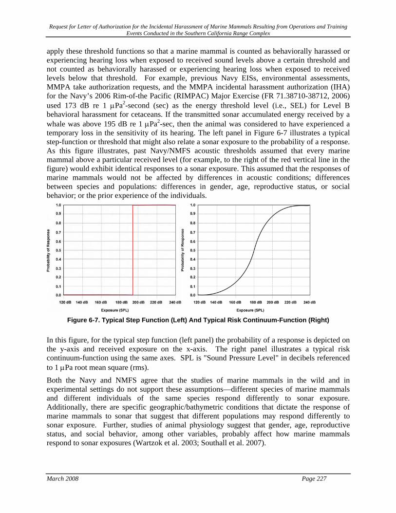
Request for Letter of Authorization for the Incidental Harassment of Marine Mammals Resulting from Operations and Training Events Conducted in the Southern California Range Complex
March 2008 Page 227
apply these threshold functions so that a marine mammal is counted as behaviorally harassed or experiencing hearing loss when exposed to received sound levels above a certain threshold and not counted as behaviorally harassed or experiencing hearing loss when exposed to received levels below that threshold. For example, previous Navy EISs, environmental assessments, MMPA take authorization requests, and the MMPA incidental harassment authorization (IHA) for the Navy’s 2006 Rim-of-the Pacific (RIMPAC) Major Exercise (FR 71.38710-38712, 2006) used 173 dB re 1 μPa2-second (sec) as the energy threshold level (i.e., SEL) for Level B behavioral harassment for cetaceans. If the transmitted sonar accumulated energy received by a whale was above 195 dB re 1 μPa2-sec, then the animal was considered to have experienced a temporary loss in the sensitivity of its hearing. The left panel in Figure 6-7 illustrates a typical step-function or threshold that might also relate a sonar exposure to the probability of a response. As this figure illustrates, past Navy/NMFS acoustic thresholds assumed that every marine mammal above a particular received level (for example, to the right of the red vertical line in the figure) would exhibit identical responses to a sonar exposure. This assumed that the responses of marine mammals would not be affected by differences in acoustic conditions; differences between species and populations: differences in gender, age, reproductive status, or social behavior; or the prior experience of the individuals.
Figure 6-7. Typical Step Function (Left) And Typical Risk Continuum-Function (Right)
In this figure, for the typical step function (left panel) the probability of a response is depicted on the y-axis and received exposure on the x-axis. The right panel illustrates a typical risk continuum-function using the same axes. SPL is "Sound Pressure Level" in decibels referenced to 1 μPa root mean square (rms).
Both the Navy and NMFS agree that the studies of marine mammals in the wild and in experimental settings do not support these assumptions—different species of marine mammals and different individuals of the same species respond differently to sonar exposure. Additionally, there are specific geographic/bathymetric conditions that dictate the response of marine mammals to sonar that suggest that different populations may respond differently to sonar exposure. Further, studies of animal physiology suggest that gender, age, reproductive status, and social behavior, among other variables, probably affect how marine mammals respond to sonar exposures (Wartzok et al. 2003; Southall et al. 2007).

Request for Letter of Authorization for the Incidental Harassment of Marine Mammals Resulting from Operations and Training Events Conducted in the Southern California Range Complex
Page 228 March 2008
Over the past several years, the Navy and NMFS have worked on developing an MFA sonar acoustic risk function to replace the acoustic thresholds used in the past to estimate the probability of marine mammals being behaviorally harassed by received levels of MFA sonar. The Navy and NMFS will continue to use acoustic thresholds to estimate temporary or permanent threshold shifts using SEL as the appropriate metric. Unlike acoustic thresholds, acoustic risk continuum functions (which are also called “exposure-response functions,” “dose-response functions,” or “stress-response functions” in other risk assessment contexts) assume that the probability of a response depends first on the “dose” (in this case, the received level of sound) and that the probability of a response increases as the “dose” increases. It is important to note that the probabilities associated with acoustic risk functions do not represent an individual’s probability of responding. Rather, the probabilities identify the proportion of an exposed population that is likely to respond to an exposure.
The right panel in Figure 6-7 illustrates a typical acoustic risk function that might relate an exposure, as received SPL in dB re 1 μPa, to the probability of a response. As the exposure receive level increases in this figure, the probability of a response increases as well but the relationship between an exposure and a response is “linear” only in the center of the curve (that is, unit increases in exposure would produce unit increases in the probability of a response only in the center of a risk function curve). In the “tails” of an acoustic risk function curve, unit increases in exposure produce smaller increases in the probability of a response. Based on observations of various animals, including humans, the relationship represented by an acoustic risk function is a more robust predictor of the probable behavioral responses of marine mammals to sonar and other acoustic sources.
The Navy and NMFS have previously used the acoustic risk function to estimate the probable responses of marine mammals to acoustic exposures for other training and research programs. Examples of previous application include the Navy Final EISs on the SURTASS LFA sonar (DoN 2001); the North Pacific Acoustic Laboratory experiments conducted off the Island of Kauai (Office of Naval Research, 2001), and the Supplemental EIS for SURTASS LFA sonar (DoN 2007a).
The Navy and NMFS used two metrics to estimate the number of marine mammals that could be subject to Level B harassment (behavioral harassment and TTS) as defined by the MMPA, during training exercises. The agencies used acoustic risk functions with the metric of received SPL (dB re 1 µPa) to estimate the number of marine mammals that might be at risk for MMPA Level B behavioral harassment as a result of being exposed to MFA sonar. The agencies will continue to use acoustic thresholds (“step-functions”) with the metric of SEL (dB re 1 µPa2-s) to estimate the number of marine mammals that might be “taken” through sensory impairment (i.e., Level A – PTS and Level B – TTS) as a result of being exposed to MFA sonar.
Although the Navy has not used acoustic risk functions in previous MFA sonar assessments of the potential effects of MFA sonar on marine mammals, risk functions are not new concepts for risk assessments. Common elements are contained in the process used for developing criteria for air, water, radiation, and ambient noise and for assessing the effects of sources of air, water, and noise pollution. The Environmental Protection Agency (EPA) uses dose-functions to develop water quality criteria and to regulate pesticide applications (U.S. EPA 1998); the Nuclear Regulatory Commission (NRC) uses dose-functions to estimate the consequences of radiation exposures (see NRC 1997 and 10 Code of Federal Regulations [C.F.R] § 20.1201); the Centers for Disease Control and Prevention (CDCP) and the Food and Drug Administration (FDA) use

Request for Letter of Authorization for the Incidental Harassment of Marine Mammals Resulting from Operations and Training Events Conducted in the Southern California Range Complex
March 2008 Page 229
dose-functions as part of their assessment methods (for example, see CDCP 2003, U.S. FDA 2001); and the Occupational Safety and Health Administration (OSHA) uses dose-functions to assess the potential effects of noise and chemicals in occupational environments on the health of people working in those environments (for examples, see FR 61:56746-56856, 1996; FR 71:10099-10385, 2006).
6.15.2 Risk Function Adapted from Feller (1968) The particular acoustic risk function developed by the Navy and NMFS estimates the probability of behavioral responses that NMFS would classify as harassment for the purposes of the MMPA given exposure to specific received levels of MFA sonar. The mathematical function is derived from a solution in Feller (1968) as defined in the SURTASS LFA Sonar Final OEIS/EIS (DoN 2001), and relied on in the Supplemental SURTASS LFA Sonar EIS (DoN 2007a) for the probability of MFA sonar risk for MMPA Level B behavioral harassment with input parameters modified by NMFS for MFA sonar for mysticetes, odontocetes, and pinnipeds.
In order to represent a probability of risk, the function should have a value near zero at very low exposures, and a value near one for very high exposures. One class of functions that satisfies this criterion is cumulative probability distributions, a type of cumulative distribution function. In selecting a particular functional expression for risk, several criteria were identified:
• The function must use parameters to focus discussion on areas of uncertainty; • The function should contain a limited number of parameters; • The function should be capable of accurately fitting experimental data; and • The function should be reasonably convenient for algebraic manipulations.
As described in DoN (2001), the mathematical function below is adapted from a solution in Feller (1968).
A
A
KBL
KBL
R 2
1
1
−
−
⎟⎠⎞
⎜⎝⎛ −
−
⎟⎠⎞
⎜⎝⎛ −
−=
Where: R = risk (0 – 1.0);
L = Received Level (RL) in dB;
B = basement RL in dB; (120 dB);
K = the RL increment above basement in dB at which there is 50 percent risk;
A = risk transition sharpness parameter (10) (explained in 3.1.5.3).
In order to use this function, the values of the three parameters (B, K, and A) need to be established. The values used in this LOA analysis are based on three sources of data: TTS experiments conducted at SSC and documented in Finneran, et al. (2001, 2003, and 2005; Finneran and Schlundt 2004); reconstruction of sound fields produced by the USS SHOUP associated with the behavioral responses of killer whales observed in Haro Strait and documented in Department of Commerce NMFS (2005); DoN (2004); and Fromm (2004a, 2004b); and observations of the behavioral response of North Atlantic right whales exposed to

Request for Letter of Authorization for the Incidental Harassment of Marine Mammals Resulting from Operations and Training Events Conducted in the Southern California Range Complex
Page 230 March 2008
alert stimuli containing mid-frequency components documented in Nowacek et al. (2004). The input parameters, as defined by NMFS, are based on very limited data that represent the best available science at this time.
6.15.3 Data Sources Used for Risk Function There is widespread consensus that cetacean response to MFA sound signals needs to be better defined using controlled experiments. Navy is contributing to an ongoing behavioral response study in the Bahamas that is anticipated to provide some initial information on beaked whales, the species identified as the most sensitive to MFA sonar. NMFS is leading this international effort with scientists from various academic institutions and research organizations to conduct studies on how marine mammals respond to underwater sound exposures.
Until additional data is available, NMFS and the Navy have determined that the following three data sets are most applicable for the direct use in developing risk function parameters for MFA/HFA sonar. These data sets represent the only known data that specifically relate altered behavioral responses to exposure to MFA sound sources.
Data from SSC’s Controlled Experiments: Most of the observations of the behavioral responses of toothed whales resulted from a series of controlled experiments, designed as acoustic experiments rather than behavioral experiments, on bottlenose dolphins and beluga whales conducted by researchers at SSC’s facility in San Diego, California (Finneran et al. 2001, 2003, 2005; Finneran and Schlundt 2004; Schlundt et al. 2000). In experimental trials with marine mammals trained to perform tasks when prompted, scientists evaluated whether the marine mammals performed these tasks when exposed to mid-frequency tones. Altered behavior during experimental trials usually involved refusal of animals to return to the site of the sound stimulus. This refusal included what appeared to be deliberate attempts to avoid a sound exposure or to avoid the location of the exposure site during subsequent tests (Schlundt et al. 2000, Finneran et al. 2002). Bottlenose dolphins exposed to 1-sec intense tones exhibited short-term changes in behavior above received sound levels of 178 to 193 dB re 1 μPa rms, and beluga whales did so at received levels of 180 to 196 dB and above.
Finneran and Schlundt (2004) examined behavioral observations recorded by the trainers or test coordinators during the Schlundt et al. (2000) and Finneran et al. (2001, 2003, 2005) experiments featuring 1-second (sec) tones. These included observations from 193 exposure sessions (fatiguing stimulus level > 141 dB re 1μPa) conducted by Schlundt et al. (2000) and 21 exposure sessions conducted by Finneran et al. (2001, 2003, 2005). The observations were made during exposures to sound sources at 0.4 kHz, 3 kHz, 10 kHz, 20 kHz, and 75 kHz. The TTS experiments that supported Finneran and Schlundt (2004) are further explained below:
Schlundt et al. (2000) provided a detailed summary of the behavioral responses of trained marine mammals during TTS tests conducted at SSC San Diego with 1-sec tones. Schlundt et al. (2000) reported eight individual TTS experiments. Fatiguing stimuli durations were 1-sec; exposure frequencies were 0.4 kHz, 3 kHz, 10 kHz, 20 kHz and 75 kHz. The experiments were conducted in San Diego Bay. Because of the variable ambient noise in the bay, low-level broadband masking noise was used to keep hearing thresholds consistent despite fluctuations in the ambient noise. Schlundt et al. (2000) reported that “behavioral alterations,” or deviations from the behaviors the animals being tested had been trained to exhibit, occurred as the animals were exposed to increasing fatiguing stimulus levels.

Request for Letter of Authorization for the Incidental Harassment of Marine Mammals Resulting from Operations and Training Events Conducted in the Southern California Range Complex
March 2008 Page 231
Finneran et al. (2001, 2003, 2005) conducted TTS experiments using tones at 3 kHz. The test method was similar to that of Schlundt et al. (2000) except the tests were conducted in a pool with very low ambient noise level (below 50 dB re 1 μPa/hertz [Hz]), and no masking noise was used. Two separate experiments were conducted using 1-sec tones. In the first, fatiguing sound levels were increased from 160 to 201 dB SPL. In the second experiment, fatiguing sound levels between 180 and 200 dB re 1 μPa were randomly presented.
Data from Studies of Baleen (Mysticetes) Whale Responses: The only mysticete data available resulted from a field experiments in which baleen whales (mysticetes) were exposed to a range frequency sound sources from 500 Hz to 4500 Hz (Nowacek et al. 2004). An alert stimulus, with a mid-frequency component, was the only portion of the study used to support the risk function input parameters.
Nowacek et al. (2004) documented observations of the behavioral response of North Atlantic right whales exposed to alert stimuli containing mid-frequency components. To assess risk factors involved in ship strikes, a multi-sensor acoustic tag was used to measure the responses of whales to passing ships and experimentally tested their responses to controlled sound exposures, which included recordings of ship noise, the social sounds of conspecifics and a signal designed to alert the whales. The alert signal was 18-minutes of exposure consisting of three 2-minute signals played sequentially three times over. The three signals had a 60 percent duty cycle and consisted of: (1) alternating 1-sec pure tones at 500 Hz and 850 Hz; (2) a 2-sec logarithmic down-sweep from 4,500 Hz to 500 Hz; and (3) a pair of low (1,500 Hz)-high (2,000 Hz) sine wave tones amplitude modulated at 120 Hz and each 1-sec long. The purposes of the alert signal were (a) to provoke an action from the whales via the auditory system with disharmonic signals that cover the whales estimated hearing range; (b) to maximize the signal to noise ratio (obtain the largest difference between background noise) and c) to provide localization cues for the whale. Five out of six whales reacted to the signal designed to elicit such behavior. Maximum received levels ranged from 133 to 148 dB re 1μPa.
Observations of Killer Whales in Haro Strait in the Wild: In May 2003, killer whales (Orcinus orca) were observed exhibiting behavioral responses while the USS SHOUP was engaged in MFA sonar operations in the Haro Strait in the vicinity of Puget Sound, Washington. Although these observations were made in an uncontrolled environment, the sound field that may have been associated with the sonar operations had to be estimated, and the behavioral observations were reported for groups of whales, not individual whales, the observations associated with the USS SHOUP provide the only data set available of the behavioral responses of wild, non-captive animal upon exposure to the AN/SQS-53 MFA sonar.
NMFS (2005), DoN (2004), and Fromm (2004a, 2004b) documented reconstruction of sound fields produced by the USS SHOUP associated with the behavioral response of killer whales observed in Haro Strait. Observations from this reconstruction included an approximate closest approach time which was correlated to a reconstructed estimate of received level at an approximate whale location (which ranged from 150 to 180 dB), with a mean value of 169.3 dB.
6.15.4 Limitations of the Risk Function Data Sources There are significant limitations and challenges to any risk function derived to estimate the probability of marine mammal behavioral responses; these are largely attributable to sparse data. Ultimately there should be multiple functions for different marine mammal taxonomic groups,

Request for Letter of Authorization for the Incidental Harassment of Marine Mammals Resulting from Operations and Training Events Conducted in the Southern California Range Complex
Page 232 March 2008
but the current data are insufficient to support them. The goal is unquestionably that risk functions be based on empirical measurement.
The risk function presented here is based on three data sets that NMFS and Navy have determined are the best available science at this time. The Navy and NMFS acknowledge each of these data sets has limitations. However, this risk function, if informed by the limited available data relevant to the MFA sonar application, has the advantages of simplicity and the fact that there is precedent for its application and foundation in marine mammal research.
While NMFS considers all data sets as being weighted equally in the development of the risk function, the Navy believes the SSC San Diego data is the most rigorous and applicable for the following reasons:
• The data represents the only source of information where the researchers had complete control over and ability to quantify the noise exposure conditions.
• The altered behaviors were identifiable due to long term observations of the animals.
• The fatiguing noise consisted of tonal exposures with limited frequencies contained in the MFA sonar bandwidth.
• However, the Navy and NMFS do agree that the following are limitations associated with the three data sets used as the basis of the risk function:
• The three data sets represent the responses of only four species: trained bottlenose dolphins and beluga whales, North Atlantic right whales in the wild and killer whales in the wild.
• None of the three data sets represent experiments designed for behavioral observations of animals exposed to MFA sonar.
• The behavioral responses of marine mammals that were observed in the wild (observations of killer whales in Haro Strait) are based on an estimated received level of sound exposure; they do not take into consideration (due to minimal or no supporting data):
• Potential relationships between acoustic exposures and specific behavioral activities (e.g., feeding, reproduction, changes in diving behavior, etc.), variables such as bathymetry, or acoustic waveguides; or
• Differences in individuals, populations, or species, or the prior experiences, reproductive state, hearing sensitivity, or age of the marine mammal.
SSC San Diego Trained Bottlenose Dolphins and Beluga Data Set: • The animals were trained animals in captivity; therefore, they may be more or less
sensitive than cetaceans found in the wild (Domjan, 1998).
• The tests were designed to measure TTS, not behavior.
• Because the tests were designed to measure TTS, the animals were exposed to much higher levels of sound than the baseline risk function (only two of the total 193 observations were at levels below 160 dB re 1 μPa2-s).
• The animals were not exposed in the open ocean but in a shallow bay or pool.

Request for Letter of Authorization for the Incidental Harassment of Marine Mammals Resulting from Operations and Training Events Conducted in the Southern California Range Complex
March 2008 Page 233
North Atlantic Right Whales in the Wild Data Set: • The observations of behavioral response were from exposure to alert stimuli that
contained mid-frequency components but was not similar to a MFA sonar ping. The alert signal was 18 minutes of exposure consisting of three 2-minute signals played sequentially three times over. The three signals had a 60 percent duty cycle and consisted of: (1) alternating 1-sec pure tones at 500 Hz and 850 Hz; (2) a 2-sec logarithmic down-sweep from 4,500 Hz to 500 Hz; and (3) a pair of low (1,500 Hz)-high (2,000 Hz) sine wave tones amplitude modulated at 120 Hz and each 1-sec long. This 18-minute alert stimuli is in contrast to the average 1-sec ping every 30 sec in a comparatively very narrow frequency band used by military sonar.
• The purpose of the alert signal was, in part, to provoke an action from the whales through an auditory stimulus.
Killer Whales in the Wild Data Set: • The observations of behavioral harassment were complicated by the fact that there
were other sources of harassment in the vicinity (other vessels and their interaction with the animals during the observation).
• The observations were anecdotal and inconsistent. There were no controls during the observation period, with no way to assess the relative magnitude of the any observed response as opposed to baseline conditions.
6.15.5 Input Parameters for the Risk Function The values of B, K, and A need to be specified in order to utilize the risk function defined in Section 3.9.7.4.2. The risk continuum function approximates the dose-response function in a manner analogous to pharmacological risk assessment (DoN 2001, Appendix A). In this case, the risk function is combined with the distribution of sound exposure levels to estimate aggregate impact on an exposed population.
6.15.6 Basement Value for Risk—The B Parameter The B parameter defines the basement value for risk, below which the risk is so low that calculations are impractical. This 120 dB level is taken as the estimate received level (RL) below which the risk of significant change in a biologically important behavior approaches zero for the MFA sonar risk assessment. This level is based on a broad overview of the levels at which multiple species have been reported responding to a variety of sound sources, both mid-frequency and other, was recommended by the scientists, and has been used in other publications. The Navy recognizes that for actual risk of changes in behavior to be zero, the signal-to-noise ratio of the animal must also be zero. However, the present convention of ending the risk calculation at 120 dB for MFA sonar has a negligible impact on the subsequent calculations, because the risk function does not attain appreciable values at received levels that low.
6.15.7 The K Parameter NMFS and the Navy used the mean of the following values to define the midpoint of the function: (1) the mean of the lowest received levels (185.3 dB) at which individuals responded with altered behavior to 3 kHz tones in the SSC data set; (2) the estimated mean received level value of 169.3 dB produced by the reconstruction of the USS SHOUP incident in which killer

Request for Letter of Authorization for the Incidental Harassment of Marine Mammals Resulting from Operations and Training Events Conducted in the Southern California Range Complex
Page 234 March 2008
whales exposed to MFA sonar (range modeled possible received levels: 150 to 180 dB); and (3) the mean of the 5 maximum received levels at which Nowacek et al. (2004) observed significantly altered responses of right whales to the alert stimuli than to the control (no input signal) is 139.2 dB SPL. The arithmetic mean of these three mean values is 165 dB SPL. The value of K is the difference between the value of B (120 dB SPL) and the 50 percent value of 165 dB SPL; therefore, K=45.
6.15.8 Risk Transition—The A Parameter The A parameter controls how rapidly risk transitions from low to high values with increasing receive level (Figures 6-8 and 6-9) . As A increases, the slope of the risk function increases. For very large values of A, the risk function can approximate a threshold response or step function. NMFS has recommended that Navy use A=10 as the value for odontocetes, and pinnipeds (NMFS 2008). This is the same value of A that was used for the SURTASS LFA sonar analysis. As stated in the SURTASS LFA Sonar Final OEIS/EIS (DoN 2001), the value of A=10 produces a curve that has a more gradual transition than the curves developed by the analyses of migratory gray whale studies (Malme et al., 1984). The choice of a more gradual slope than the empirical data was consistent with other decisions for the SURTASS LFA Sonar Final OEIS/EIS to make conservative assumptions when extrapolating from other data sets (see Subchapter 1.43 and Appendix D of the SURTASS LFA Sonar OEIS/EIS [NMFS 2008]).
Based on NMFS’ direction, the Navy will use a value of A=8 for mysticetes to allow for greater consideration of potential harassment at the lower received levels based on Nowacek et al., 2004 (NMFS 2008).
120 130 140 150 160 170 180 1900
0.1
0.2
0.3
0.4
0.5
0.6
0.7
0.8
0.9
1
Received Level (dB)
Pro
babi
lity
of H
aras
smen
t
Figure 6-8. Risk Function Curve for Odontocetes (Toothed Whales) and Pinnipeds
50% Risk at 165 dB SPL
A = 10
K = 45 dB SPL
B = 120 dB SPL

Request for Letter of Authorization for the Incidental Harassment of Marine Mammals Resulting from Operations and Training Events Conducted in the Southern California Range Complex
March 2008 Page 235
120 130 140 150 160 170 180 1900
0.1
0.2
0.3
0.4
0.5
0.6
0.7
0.8
0.9
1
Received Level (dB)
Pro
babi
lity
of H
aras
smen
t
Figure 6-9. Risk Function Curve for Mysticetes (Baleen Whales)
6.15.9 Application of the Risk Function and Current Regulatory Scheme The risk function is used to estimate the percentage of an exposed population that is likely to exhibit behaviors that would qualify as harassment (as that term is defined by the MMPA applicable to military readiness activities, such as the Navy’s testing and training with mid- and high-frequency active sonar) at a given received level of sound. For example, at 165 dB SPL (dB re: 1µPa rms), the risk (or probability) of harassment is defined according to this function as 50 percent, and Navy/NMFS applies that by estimating that 50 percent of the individuals exposed at that received level are likely to respond by exhibiting behavior that NMFS would classify as behavioral harassment. The risk function is not applied to individual animals, only to exposed populations. The data used to produce the risk function were compiled from four species that had been exposed to sound sources in a variety of different circumstances. As a result, the risk function represents a general relationship between acoustic exposures and behavioral responses that is then applied to specific circumstances. That is, the risk function represents a relationship that is deemed to be generally true, based on the limited, best-available science, but may not be true in specific circumstances. In particular, the risk function, as currently derived, treats the received level as the only variable that is relevant to a marine mammal’s behavioral response. However, we know that many other variables—the marine mammal’s gender, age, and prior experience; the activity it is engaged in during an exposure event, its distance from a sound source, the number of sound sources, and whether the sound sources are approaching or moving away from the animal—can be critically important in determining whether and how a marine mammal will respond to a sound source (Southall et al. 2007). The data that are currently
50% Risk at 165 dB SPL
A = 8
K = 45 dB SPL
B = 120 dB SPL

Request for Letter of Authorization for the Incidental Harassment of Marine Mammals Resulting from Operations and Training Events Conducted in the Southern California Range Complex
Page 236 March 2008
available do not allow for incorporation of these other variables in the current risk functions; however, the risk function represents the best use of the data that are available.
As more specific and applicable data become available, NMFS can use these data to modify the outputs generated by the risk function to make them more realistic (and ultimately, data may exist to justify the use of additional, alternate, or multi-variate functions). As mentioned above, it is known that the distance from the sound source and whether it is perceived as approaching or moving away can affect the way an animal responds to a sound (Wartzok et al. 2003). Though there are data showing marine mammal responses to sound sources at that received level, NMFS does not currently have any data that describe the response of marine mammals to sounds at that distance (or to other contextual aspects of the exposure, such as the presence of higher frequency harmonics), much less data that compare responses to similar sound levels at varying distances. However, if data were to become available that suggested animals were less likely to respond (in a manner NMFS would classify as harassment) to certain levels beyond certain distances, or that they were more likely to respond at certain closer distances, Navy will re-evaluate the risk function to try to incorporate any additional variables into the “take” estimates.
Last, pursuant to the MMPA, an applicant is required to estimate the number of animals that will be “taken” by their activities. This estimate informs the analysis that NMFS must perform to determine whether the activity will have a “negligible impact” on the species or stock. Level B (behavioral) harassment occurs at the level of the individual(s) and does not assume any resulting population-level consequences, though there are known avenues through which behavioral disturbance of individuals can result in population-level effects. Alternately, a negligible impact finding is based on the lack of likely adverse effects to annual rates of recruitment or survival (i.e., population-level effects). An estimate of the number of Level B harassment takes, alone, is not enough information on which to base an impact determination. In addition to considering estimates of the number of marine mammals that might be “taken” through harassment, NMFS must consider other factors, such as the nature of any responses (their intensity, duration, etc.), the context of any responses (critical reproductive time or location, migration, etc.), or any of the other variables mentioned in the first paragraph (if known), as well as the number and nature of estimated Level A takes, the number of estimated mortalities, and effects on habitat. For example, in the case of sonar usage in the SOCAL Range Complex, a portion of the animals that are likely to be “taken” through behavioral harassment are expected to be exposed at relatively low received levels (120-140 dB SPL) where the significance of those responses would be reduced because of the distance (25-65 nm) from a sound source. Alternatively, only a relatively very small portion (<5%) of the animals that are expected to be “taken” through behavioral harassment are expected to occur when animals are exposed to higher received levels, such as the onset of TTS (195 dB re 1 μPa2-s) or higher. Since the modeling does not take into account the reduction of effects resulting from the Navy’s standard mitigation, approximately 25% of all exposures are modeled as having occurred within the 1,000 yard mitigation safety zone where procedures are in place to reduce the received level of animals within this zone. Generally speaking, Navy and NMFS anticipate more severe effects from takes resulting from exposure to higher received levels (though this is in no way a strictly linear relationship throughout species, individuals, or circumstances) and less severe effects from takes resulting from exposure to lower received levels.
It is worth noting that Navy and NMFS would expect an animal exposed to the levels at the bottom of the risk function to exhibit behavioral responses that are less likely to adversely affect

Request for Letter of Authorization for the Incidental Harassment of Marine Mammals Resulting from Operations and Training Events Conducted in the Southern California Range Complex
March 2008 Page 237
the longevity, survival, or reproductive success of the animals that might be exposed, based on received level, and the fact that the exposures will occur in the absence of some of the other contextual variables that would likely be associated with increased severity of effects, such as the proximity of the sound source(s) or the proximity of other vessels, aircraft, submarines, etc. maneuvering in the vicinity of the exercise. NMFS will consider all available information (other variables, etc.), but all else being equal, takes that result from exposure to lower received levels and at greater distances from the exercises would be less likely to contribute to population level effects.
6.15.10 Navy Protocols For Acoustic Modeling Analysis of Marine Mammal Exposures
Previous variations of the Navy’s acoustic impact model allowed for significant overestimation of potential exposures based on a series of assumptions that now have more precise resolution. Specifically in the past, the model overestimated effects because:
• Acoustic footprints for sonar sources near land are not reduced to account for the land mass where marine mammals would not occur.
• Acoustic footprints for sonar sources were added independently and, therefore, did not account for overlap they would have with other sonar systems used during the same active sonar activity. As a consequence, the area of the total acoustic footprint was larger than the actual acoustic footprint when multiple ships are operating together.
• Acoustic exposures do not reflect implementation of mitigation measures, such as reducing sonar source levels when marine mammals are present.
• Marine mammal densities were averaged across specific active sonar activity areas and, therefore, are evenly distributed without consideration for animal grouping or patchiness.
• Acoustic modeling did not account for limitations of the NMFS-defined refresh rate of 24 hours. This time period represents the amount of time in which individual marine mammals can be harasses no more than once.
Table 6-2 provides a summary of the modeling protocols used in the analysis for this LOA.

Request for Letter of Authorization for the Incidental Harassment of Marine Mammals Resulting from Operations and Training Events Conducted in the Southern California Range Complex
Page 238 March 2008
Table 6-2. Navy Protocols Providing for Modeling Quantification of Marine Mammal Exposures
Historical Data
Sonar Positional Reporting System
(SPORTS)
Annual active sonar usage data will be obtained from the SPORTS database to determine the number of active sonar hours and the
geographic location of those hours for modeling purposes.
AN/SQS-53 and AN/SQS-56
Model the AN/SQS-53 and the AN/SQS-56 active sonar sources separately to account for the differences in source level, frequency,
and exposure effects. Acoustic Parameters
Submarine Sonar Submarine active sonar use will be included in effects analysis calculations using the SPORTS database.
Land Shadow For sound sources within the acoustic footprint of land, subtract the land area from the marine mammal exposure calculation.
Multiple Ships Correction factors will be used to address overestimates of
exposures to marine mammals resulting from multiple counting when there are more than one ship operating in the same vicinity.
Post Modeling Analysis
Multiple Exposures
The following refresh rates for SOCAL Range Complex training events will be included to account for multiple exposures:
Unit-level Training, Coordinated Events, and Maintenance – 4 hours
Integrated Anti-submarine Warfare (ASW) Course- – 16 hours Major Exercises / Major Range Events– 12 hours
Sustainment Training Exercises – 12 hours.
6.16 Other Effects Considered 6.16.1 Stress A possible stressor for marine mammals exposed to sound, including mid-frequency active sonar, is the effect on health and physiological stress (Review by Fair and Becker 2000). A stimulus may cause a number of behavioral and physiological responses such as an elevated heart rate, increases in endocrine and neurological function, and decreased immune function, particularly if the animal perceives the stimulus as life threatening (Seyle 1950; Moberg 2000; Sapolsky et al. 2005). The primary response to the stressor is to move away to avoid continued exposure. Next, the animal’s physiological response to a stressor is to engage the autonomic nervous system with the classic “fight or flight” response. This includes changes in the cardiovascular system (increased heart rate), the gastrointestinal system (decrease digestion), the exocrine glands (increased hormone output), and the adrenal glands (increased nor-epinephrine). These physiological and hormonal responses are short lived and may not have significant long-term effects on an animal’s health or fitness. Generally these short term responses are not detrimental to the animal except when the health of the animal is already compromised by disease, starvation or parasites; or the animal is chronically exposed to a stressor.
Exposure to chronic or high intensity sound sources can cause physiological stress. Acoustic exposures and physiological responses have been shown to cause stress responses (elevated respiration and increased heart rates) in humans (Jansen 1998). Jones (1998) reported on

Request for Letter of Authorization for the Incidental Harassment of Marine Mammals Resulting from Operations and Training Events Conducted in the Southern California Range Complex
March 2008 Page 239
reductions in human performance when faced with acute, repetitive exposures to acoustic disturbance. Trimper et al. (1998) reported on the physiological stress responses of osprey to low-level aircraft noise. Krausman et al. (2004) reported on the auditory (TTS) and physiology stress responses of endangered Sonoran pronghorn to military overflights. Smith et al. (2004a, 2004b) recorded sound-induced physiological stress responses in a hearing-specialist fish that was associated with TTS. Welch and Welch (1970) reported physiological and behavioral stress responses that accompanied damage to the inner ears of fish and several mammals.
Most of these responses to sound sources or other stimuli have been studied extensively in terrestrial animals but are much more difficult to determine in marine mammals. Increases in heart rate are common reaction to acoustic disturbance in marine mammals (Miksis et al. 2001) as are small increases in the hormones norepinephrine, epinephrine, and dopamine (Romano et al. 2002; 2004). Increases in cortical steroids are more difficult to determine because blood collection procedures will also cause stress (Romano et al. 2002; 2004). A recent study, Chase Encirclement Stress Studies (CHESS), was conducted by NMFS on chronic stress effects in small odontocetes affected by the eastern tropical Pacific (ETP) tuna fishery (Forney et al. 2002). Analysis was conducted on blood constituents, immune function, reproductive parameters, heart rate and body temperature of small odontocetes that had been pursued and encircled by tuna fishing boats. Some effects were noted, including lower pregnancy rates, increases in norepinephrine, dopamine, ACTH and cortisol levels, heart lesions and an increase in fin and surface temperature when chased for over 75 minutes but with no change in core body temperature (Forney et al. 2002). These stress effects in small cetaceans that were actively pursued (sometimes for over 75 minutes) were relatively small and difficult to discern. It is unlikely that marine mammals exposed to mid-frequency active sonar would be exposed at long as the cetaceans in the CHESS study and would not be pursued by the Navy ships, therefore stress effects would be minimal from the short term exposure to sonar.
6.16.2 Acoustically Mediated Bubble Growth One suggested cause of injury to marine mammals is by rectified diffusion (Crum and Mao 1996) the process of increasing the size of a bubble by exposing it to a sound field. This process is facilitated if the environment in which the ensonified bubbles exist is supersaturated with a gas, such as nitrogen which makes up approximately 78 percent of air (remainder of air is about 21 percent oxygen with some carbon dioxide). Repetitive diving by marine mammals can cause the blood and some tissues to accumulate gas to a greater degree than is supported by the surrounding environmental pressure (Ridgway and Howard 1979). Deeper and longer dives of some marine mammals (for example, beaked whales) are theoretically predicted to induce greater super saturation (Houser et al. 2001). Conversely, studies have shown that marine mammal lung structure (both pinnipeds and cetaceans) facilitates collapse of the lungs at depths deeper than approximately 162 ft (Kooyman et al. 1970). Collapse of the lungs would force air in to the non-air exchanging areas of the lungs (in to the bronchioles away from the alveoli) thus significantly decreasing nitrogen diffusion in to the body. Deep diving pinnipeds such as the northern elephant and Weddell seals (Leptonychotes weddellii) typically exhale before long deep dives, further reducing air volume in the lungs (Kooyman et al. 1970). If rectified diffusion were possible in marine mammals exposed to high-level sound, conditions of tissue super saturation could theoretically speed the rate and increase the size of bubble growth. Subsequent effects due to tissue trauma and emboli would presumably mirror those observed in humans suffering from decompression sickness.

Request for Letter of Authorization for the Incidental Harassment of Marine Mammals Resulting from Operations and Training Events Conducted in the Southern California Range Complex
Page 240 March 2008
It is unlikely that the short duration of sonar pings would be long enough to drive bubble growth to any substantial size, if such a phenomenon occurs. However, an alternative but related hypothesis has also been suggested. Stable bubbles could be destabilized by high-level sound exposures such that bubble growth then occurs through static diffusion of gas out of the tissues. In such a scenario the marine mammal would need to be in a gas-supersaturated state for a long enough period of time and exposed to a continuous sound source for bubbles to become of a problematic size.
6.16.3 DecompressionSickness Another hypothesis suggests that rapid ascent to the surface following exposure to a startling sound might produce tissue gas saturation sufficient for the evolution of nitrogen bubbles (Jepson et al., 2003). In this scenario, the rate of ascent would need to be sufficiently rapid to compromise behavioral or physiological protections against nitrogen bubble formation. Cox et al. (2006) with experts in the field of marine mammal behavior, diving, physiology, respiration physiology, pathology, anatomy, and bio-acoustics considered this to be a plausible hypothesis but requires further investigation. Rommel et al. (2006) reviewed beaked whale anatomy and diving physiology in relation to strandings and concluded that "" It is important to note that no current hypothesis of pathogenic mechanisms resulting in acoustically-related strandings is proven." Conversely Fahlman et al., (2006) suggested that diving bradycardia (reduction in heart rate and circulation to the tissues), lung collapse and slow ascent rates would reduce nitrogen uptake and thus reduce the risk of decompression sickness by 50 percent in models of marine mammals. Zimmer and Tyack (2007) suggest that beaked whales avoid sonar sound by swimming deeper than 25 m and shallower than the depth of alveolar collapse. This avoidance mechanism continues until the sound no longer creates the response or the animal enters shallow water where it can no longer dive in this pattern. This hypothesis could lead to decompression sickness and is consistent with previous studies on avoidance, for example with ship noise (Zimmer and Tyack, 2007). Recent information on the diving profiles of Cuvier’s (Ziphius cavirostris) and Blainvilles’s (Mesoplodon densirostris) beaked whales (Baird et al., 2006) and in the Ligurian Sea in Italy (Tyack et al., 2006) showed that while these species do dive deeply (regularly exceed depths of 800 m [2,625 ft]) and for long periods (48-68 minutes), they have significantly slower ascent rates than descent rates. This fits well with Fahlman et al. (2006) model of deep and long duration divers that would have slower ascent rates to reduce nitrogen saturation and reduce the risk of decompression sickness. Therefore, if nitrogen saturation remains low, then a rapid ascent in response to sonar should not cause decompression sickness. Currently it is not known if beaked whales rapidly ascend in response to sonar or other disturbances. It may be that deep diving animals would be better protected diving to depth to avoid predators, such as killer whales, rather then ascending to the surface where they may be more susceptible to predators.
Although theoretical predictions suggest the possibility for acoustically mediated bubble growth, there is considerable disagreement among scientists as to its likelihood (Piantadosi and Thalmann, 2004; Evans and Miller, 2004). To date, ELs predicted to cause in vivo bubble formation within diving cetaceans have not been evaluated (NOAA, 2002b). Further, although it has been argued that traumas from recent beaked whale strandings are consistent with gas emboli and bubble-induced tissue separations (Jepson et al., 2003), there is no conclusive evidence of this and complicating factors associated with introduction of gas in to the venous system during necropsy. Because evidence supporting it is debatable, no marine mammals addressed in this
Request for Letter of Authorization for the Incidental Harassment of Marine Mammals Resulting from Operations and Training Events Conducted in the Southern California Range Complex
March 2008 Page 241
LOA are given special treatment due to the possibility for acoustically mediated bubble growth. Beaked whales are, however, assessed differently from other species to account for factors that may have contributed to prior beaked whale strandings as set out in the previous section.
6.16.4 Resonance Another suggested cause of injury in marine mammals is air cavity resonance due to sonar exposure. Resonance is a phenomenon that exists when an object is vibrated at a frequency near its natural frequency of vibration—the particular frequency at which the object vibrates most readily. The size and geometry of an air cavity determine the frequency at which the cavity will resonate. Displacement of the cavity boundaries during resonance has been suggested as a cause of injury. Large displacements have the potential to tear tissues that surround the air space (for example, lung tissue).
Understanding resonant frequencies and the susceptibility of marine mammal air cavities to resonance is important in determining whether certain sonars have the potential to affect different cavities in different species. In 2002, NMFS convened a panel of government and private scientists to address this issue (NOAA 2002b). They modeled and evaluated the likelihood that Navy mid-frequency active sonar caused resonance effects in beaked whales that eventually led to their stranding (DOC and DoN 2001). The conclusions of that group were that resonance in air-filled structures the frequencies at which resonance were predicted to occur were below the frequencies utilized by the sonar systems employed. Furthermore, air cavity vibrations due to the resonance effect were not considered to be of sufficient amplitude to cause tissue damage.
6.16.5 Likelihood of Prolonged Exposure The proposed ASW activities within the SOCAL Range Complex would not result in prolonged exposure because the vessels are constantly moving, and the flow of the activity in the SOCAL Range Complex when ASW training occurs reduces the potential for prolonged exposure. The implementation of the mitigation measures described in Section 11 would further reduce the likelihood of any prolonged exposure.
6.16.6 Likelihood of Masking Natural and artificial sounds can disrupt behavior by masking, or interfering with an animal’s ability to hear other sounds. Masking occurs when the receipt of a sound is interfered with by a second sound at similar frequencies and at similar or higher levels. If the second sound were artificial, it could be potentially harassing if it disrupted hearing-related behavior such as communications or echolocation. It is important to distinguish TTS and PTS, which persist after the sound exposure, from masking, which occurs during the sound exposure.
Historically, principal masking concerns have been with prevailing background sound levels from natural and manmade sources (for example, Richardson et al. 1995). Dominant examples of the latter are the accumulated sound from merchant ships and sound of seismic surveys. Both cover a wide frequency band and are long in duration.
The proposed SOCAL Range Complex ASW areas are away from harbors but may include heavily traveled shipping lanes, although shipping lanes are a small portion of the overall range complex. The loudest mid-frequency underwater sounds in the Proposed Action area are those produced by hull-mounted mid-frequency active tactical sonar. The sonar signals are likely within the audible range of most cetaceans, but are very limited in the temporal and frequency

Request for Letter of Authorization for the Incidental Harassment of Marine Mammals Resulting from Operations and Training Events Conducted in the Southern California Range Complex
Page 242 March 2008
domains. In particular, the pulse lengths are short, the duty cycle low, the total number of hours of operation per year small, and these hull-mounted mid-frequency active tactical sonars transmit within a narrow band of frequencies (typically less than one-third octave).
For the reasons outlined above, the chance of sonar operations causing masking effects is considered negligible.
6.16.7 Long-Term Effects Navy activities are conducted in the same general areas throughout the SOCAL Range Complex, so marine mammal populations could be exposed to repeated activities over time. However, as described earlier, short-term non-injurious sound exposure levels predicted to cause TTS or temporary behavioral disruptions qualify as Level B harassment. Application of this criterion assumes an effect even though it is highly unlikely that all behavioral disruptions or instances of TTS will result in long term significant impacts.
Long-term monitoring programs for the SOCAL Range Complex are being developed by the Navy to assess population trends and responses of marine mammals to Navy activities. Short-term monitoring programs for exercises (e.g., undersea warfare exercise (USWEX)) are being developed to assess mitigation measures and responses of marine mammals to Navy activities.
6.17 Application of Exposure Thresholds to Other Species Mysticetes Information on auditory function in mysticetes is extremely lacking. Sensitivity to low-frequency sound by baleen whales has been inferred from observed vocalization frequencies, observed reactions to playback of sounds, and anatomical analyses of the auditory system. Baleen whales are estimated to hear from 15 Hz to 20 kHz, with good sensitivity from 20 Hz to 2 kHz (Ketten 1998). Filter-bank models of the humpback whale’s ear have been developed from anatomical features of the humpback’s ear and optimization techniques (Houser et al. 2001). The results suggest that humpbacks are sensitive to frequencies between 40 Hz and 16 kHz, but best sensitivity is likely to occur between 100 Hz and 8 kHz. However, absolute sensitivity has not been modeled for any baleen whale species. Furthermore, there is no indication of what sorts of sound exposure produce threshold shifts in these animals.
The criteria and thresholds for PTS and TTS developed for odontocetes for this activity are also used for mysticetes. This generalization is based on the assumption that the empirical data at hand are representative of both groups until data collection on mysticete species shows otherwise. For the frequencies of interest for this action, there is no evidence that the total amount of energy required to induce onset-TTS and onset-PTS in mysticetes is different than that required for odontocetes.
Beaked Whales Recent beaked whale strandings have prompted inquiry into the relationship between high-amplitude continuous-type sound and the cause of those strandings. For example, in the stranding in the Bahamas in 2000, the Navy mid-frequency sonar was identified as the only contributory cause that could have lead to the stranding. The Bahamas exercise entailed multiple ships using mid-frequency sonar during transit of a long constricted channel. The Navy participated in an extensive investigation of the stranding with the NMFS. The “Joint Interim Report, Bahamas Marine Mammal Stranding Event of 15-16 March 2000” concluded that the

Request for Letter of Authorization for the Incidental Harassment of Marine Mammals Resulting from Operations and Training Events Conducted in the Southern California Range Complex
March 2008 Page 243
variables to be considered in managing future risk from tactical mid-range sonar were “sound propagation characteristics (in this case a surface duct), unusual underwater bathymetry, intensive use of multiple sonar units, a constricted channel with limited egress avenues, and the presence of beaked whales that appear to be sensitive to the frequencies produced by these sonars.” (DOC and DoN 2001).
The Navy analyzed the known range of operational, biological, and environmental factors involved in the Bahamas stranding and focused on the interplay of these factors to reduce risks to beaked whales from ASW training operations. The confluence of these factors do not occur in the SOCAL Range Complex. Although beaked whales are visually and acoustically detected in areas where sonar use routinely takes place, there has not been a stranding of beaked whales in the SOCAL Range Complex associated with the 30-year use history of the present sonar systems.
This history would suggest that the simple exposure of beaked whales to sonar is not enough to cause beaked whales to strand. Brownell et al (2004), have suggested that the high number of beaked whale strandings in Japan between 1980 and 2004 may be related to U.S. Navy sonar use in those waters given the presence of U.S. Naval Bases and exercises off Japan. The Center for Naval Analysis compiled the history of naval exercises taking place off Japan and found there to be no correlation in time for any of the stranding events presented in Brownell et al (2004). Like the situation in California, there are clearly beaked whales present in the waters off Japan (as evidenced by the strandings) however, there is no correlation in time to strandings and sonar use. Sonar did not causing the strandings provided by Brownell et al. (2004) and more importantly, this suggests sonar use in the presence of beaked whales over two decades has not resulted in strandings related to sonar use.
As suggested by the known presence of beaked whales in waters sonar use has historically taken place, it is likely that beaked whales have been occasionally exposed to sonar during the last 30 years of sonar use in Southern California and yet there is no indication of any adverse impact on beaked whales from exposure to sonar in Californian waters. Therefore, the continued use of sonar in the SOCAL Range Complex is not likely to result in effects to beaked whales.
6.17.1 Explosive Source Criteria The criterion for mortality for marine mammals used in the CHURCHILL FEIS (DoN, 2001) is “onset of severe lung injury.” This is conservative in that it corresponds to a 1 percent chance of mortal injury, and yet any animal experiencing onset severe lung injury is counted as a lethal exposure.
The threshold is stated in terms of the Goertner (1982) modified positive impulse with value “indexed to 31 psi-ms.'” Since the Goertner approach depends on propagation, source/animal depths, and animal mass in a complex way, the actual impulse value corresponding to the 31-psi-ms index is a complicated calculation. Again, to be conservative, CHURCHILL used the mass of a calf dolphin (at 12.2 kg), so that the threshold index is 30.5 psi-ms (Table 6.3).
Two criteria are used for injury: onset of slight lung hemorrhage and 50 percent eardrum rupture (tympanic membrane [TM] rupture). These criteria are considered indicative of the onset of injury (Table 6.3).

Request for Letter of Authorization for the Incidental Harassment of Marine Mammals Resulting from Operations and Training Events Conducted in the Southern California Range Complex
Page 244 March 2008
Table 6-3. Effects Analysis Criteria for Underwater Detonations for Explosives < 2000 lbs Net Explosive Weight. Based on CHURCHILL FEIS (DoN 2001) and Eglin Air Force Base IHA (NMFS
2005h) and LOA (NMFS 2006a). Criterion Metric Threshold Comments Source
Mortality Onset of
extensive lung hemorrhage
Shock Wave Goertner modified positive impulse
30.5 psi-msec
All marine mammals
(dolphin calf)
Goertner 1982
Slight Injury Onset of slight
lung hemorrhage
Shock Wave Goertner modified positive impulse
13.0 psi-msec
All marine mammals
(dolphin calf)
Goertner 1982
Mor
talit
y &
Inju
ry
Slight Injury 50% TM Rupture
Shock Wave Energy Flux Density (EFD) for any single
exposure
205 dB re:1µPa2-sec
All marine mammals DoN 2001
Temporary Auditory Effects
TTS
Noise Exposure greatest EFD in any 1/3-octave band over
all exposures
182 dB re:1µPa2-sec
For odontocetes greatest EFD for
frequencies ≥100 Hz and for
mysticetes ≥10 Hz
NMFS 2005, NMFS 2006a
Temporary Auditory Effects
TTS
Noise Exposure Peak Pressure for any
single exposure 23 psi-msec All marine
mammals NMFS 2005
Har
assm
ent
Behavioral Modification
Noise Exposure greatest EFD in any 1/3-octave band over
all exposures
177 dB re:1µPa2-sec
For odontocetes greatest EFD for
frequencies ≥100 Hz and for
mysticetes ≥10 Hz
NMFS
Notes: Goertner, J.F. 1982. Prediction of underwater explosion safe ranges for sea mammals. Naval Surface Weapons Center, White Oak Laboratory, Silver Spring, MD. NSWC/WOL TR-82-188. 25 pp. DoN. 2001. USS Churchill Shock Trail FEIS- February 2001. Department of the Navy. NMFS. 2005. Notice of Issuance of an Incidental Harassment Authorization, Incidental to Conducting the Precisions Strike Weapon (PSW) Testing and Training by Eglin Air Force Base in the Gulf of Mexico. Federal Register,70(160):48675-48691. NMFS. 2006. Incidental Takes of Marine Mammals Incidental to Specified Activities; Naval Explosive Ordnance Disposal School Training Operations at Eglin Air Force Base, Florida, National Oceanic and Atmospheric Administration, National Marine Fisheries Service. Federal Register 71(199):60693-60697 NMFS. Briefed to NMFS for VAST-IMPASS; U.S. Air Force uses 176 dB for permit applications at Eglin Gulf Test and Training Range (EGTTR)
The threshold for onset of slight lung injury is calculated for a small animal (a dolphin calf weighing 27 lb), and is given in terms of the “Goertner modified positive impulse,” indexed to 13 psi-ms in the (DoN, 2001a). This threshold is conservative since the positive impulse needed to cause injury is proportional to animal mass, and therefore, larger animals require a higher impulse to cause the onset of injury.
The threshold for TM rupture corresponds to a 50 percent rate of rupture (i.e., 50 percent of animals exposed to the level are expected to suffer TM rupture); this is stated in terms of an EL value of 205 dB re 1 μPa2-s. The criterion reflects the fact that TM rupture is not necessarily a serious or life-threatening injury, but is a useful index of possible injury that is well correlated with measures of permanent hearing impairment (e.g., Ketten, 1998 indicates a 30 percent incidence of permanent threshold shift [PTS] at the same threshold).

Request for Letter of Authorization for the Incidental Harassment of Marine Mammals Resulting from Operations and Training Events Conducted in the Southern California Range Complex
March 2008 Page 245
Two criteria are considered for non-injurious harassment temporary threshold shift (TTS), which is a temporary, recoverable, loss of hearing sensitivity (NMFS 2001; DoN 2001a).
The first criterion for TTS is 182 dB re 1 μPa2-s maximum EL level in any 1/3-octave band at frequencies >100 hertz (Hz).
A second criterion for estimating TTS threshold has also been developed. A threshold of 12 pounds per square inch (psi) peak pressure was developed for 10,000 pound charges as part of the CHURCHILL Final EIS (DoN 2001a, [FR70/160, 19 Aug 05; FR 71/226, 24 Nov 06]). It was introduced to provide a more conservative safety zone for TTS when the explosive or the animal approaches the sea surface (for which case the explosive energy is reduced but the peak pressure is not). Navy policy is to use a 23 psi criterion for explosive charges less than 1,500 lb and the 12 psi criterion for explosive charges larger than 2,000 lb. Where explosive charges fall between 1,500-2,000 lb, the application of the 23 psi will be treated on an individual bases until NMFS rules on Navy proposed use of the criteria. This is below the level of onset of TTS for an odontocete (Finneran et al. 2002). All explosives modeled for the SOCAL Range Complex EIS/OEIS are less than 1,500 lbs. Table 6-3 summarizes explosive effects criteria.
6.17.2 Shallow Water Underwater Detonations (Offshore of San Clemente Island) Navy Special Warfare (NSW) incorporates VSW, bottom-laid explosives training into Basic Underwater Demolition/School (BUD/S) and Maritime Operations (MAROPs) training curriculums. Personnel training includes small, single and multiple charges at Northwest Harbor on San Clemente Island (SCI) (Figure 6-11).
Figure6-10. San Clemente Island, Northwest Harbor Aerial Photo And Chart Depths In Fathoms At
Mean Lower Low Water

Request for Letter of Authorization for the Incidental Harassment of Marine Mammals Resulting from Operations and Training Events Conducted in the Southern California Range Complex
Page 246 March 2008
Figure 6-11. San Clemente Island, Horse Beach Cove, Aerial Photo And Chart Depths In Fathoms
At Mean Lower Low Water
These exercises are the culmination of theoretical and practical instruction for successive groups of Navy Special Warfare (NSW) personnel-in-training. The exercises are essential in that they provide NSW personnel with hands-on experience with the design, deployment, and detonation of underwater clearance devices of the general type and size that they are required to understand and utilize. The specific explosive elements and their arrangements have been selected to include the widest range of features, so that a trained operator can competently use similar forms or configurations as objectives require. That is, the explosive configurations used in the training exercises are not necessarily those that would be used in actual operations.
There are three underwater explosive exercises conducted in Northwest Harbor: the single charge (SC) exercise, the multiple-charge obstacle loading (OL) exercise, and the multiple-charge mat-weave (MW) exercise. Only SC exercises are conducted at Horse Beach Cove. Single charges of up to 20 lbs of C4 high-explosive are detonated in near-shore waters of 5 to 20 feet depth at Northwest Harbor and of 10-12 ft depth at Horse Beach Cove.
OL exercise is conducted up to 7 times a year at Northwest Harbor (Figure 6-12). The obstacles used in training are 8, 1 m2 concrete blocks on the bottom in about 15 ft of water. They are arranged in an elongated pattern parallel to the shoreline. Onto each obstacle are attached 2 haversack charges of C4 explosive weighing 20 lbs each that is equivalent to about 27 lbs of TNT. All haversacks of all obstacles are cross-connected by detonation cord to effect coordinated detonation of C4.
Figure 6-12. Obstacle Pattern

Request for Letter of Authorization for the Incidental Harassment of Marine Mammals Resulting from Operations and Training Events Conducted in the Southern California Range Complex
March 2008 Page 247
MW exercise is conducted up to 7 times a year at Northwest Harbor (Figure 6-8). Two MW devices or mats are used in training, and involves the detonation of two lattices of line-charge explosive in quick succession. Each mat is a square lattice arrangement of 2.75-in diameter line-charge high explosive with 10, 25-ft long segments arranged in a 5 x 5 cross-hatch pattern and tied together at their intersections (Figure 3-12 Square Mats). Each of the 10 line charges contains 50 lbs of PBX composite-explosive that is equivalent to about 67 lbs of TNT. The two 500-lb mats are placed side-by-side on the bottom at a depth of about 5 ft just off the shoreline. The explosive within each mat is detonated simultaneously – at the speed of the explosive – and the two mats are detonated sequentially with a time-separation of about 500 ms. By design, a mat directs a large proportion of its explosive force vertically – i e., down into the substrate and, incidentally, up into the air. MW exercises occur at the location labeled “Loc 3” on the chart in Figure 2 of the main text.
All scheduling, safety regulation enforcement, explosive handling, and explosive detonations are carried out by qualified NSW training personnel.
Mitigation Considerations and Precedence: The unusual physical topographies, the low numbers of protected species and the training routines at both sites combine with the unusual pressure-wave propagation characteristics of the Northwest Harbor, where multiple charges are used, to allow exceptionally reliable and effective mitigation procedures. Each of those characteristics will be described, but the exceptional reliability of visual detection of protected species at these sites allows for complete mitigation within a radius that extends out to the distance at which only the lowest degree of temporary auditory threshold shift (onset-TTS) would be expected to occur. That is, the procedures to be described will mitigate the potential for Level-A harassment by injury and Level-B harassment associated with TTS by not detonating explosives while protected species are in the area associated with those effects. That approach and the analysis used in this LOA for underwater explosive effects on marine mammals and turtles are based on the criteria established in the FEIS for shock trial of the USS Winston S. Churchill (DoN, 2001) and the associated regulatory ruling (66 FR 22450, May 4, 2001). From those precedents, the distance at which onset-TTS, a Level-B harassment, would be expected to occur is taken be the greater of the distances at which either the peak-pressure has fallen to 12 psi or the energy in the 3rd octave-band of highest energy has fallen to 182 dB re 1 µPa2 ·sec. For mysticetes, only energy occurring above 10 Hz was considered in the energy estimates and for odontocetes, only energy occurring above 100 Hz was considered.
Given effective mitigation to the distance associated with onset-TTS, more severe impacts – e. g., greater TTS and Level-A harassment by injury - and their associated pressure-wave metrics are not analyzed or described in this LOA. Additionally, as in the cited precedence, detonations in the SC, OL, and MW exercises occur infrequently and are isolated in time from one another so that resultant behavioral disturbance or disruption, other than that caused by TTS, does not reach the degree associated with Level-B harassment. While the OL and MW exercises usually take place on separate days over a two-day period, they may occur several hours apart on the same day. There is an average of almost 2 months between successive occurrences of this pair of exercises.
As separate criteria for carnivora (sea lions) and chelonia (turtles) have not been established, the dual criterion for odontocetes is taken, as in the cited precedence, to be protective of those groups. Recent suggested revisions to the cited precedence for large deep-water explosions are described below.

Request for Letter of Authorization for the Incidental Harassment of Marine Mammals Resulting from Operations and Training Events Conducted in the Southern California Range Complex
Page 248 March 2008
Topographic, Water, and Bottom Conditions: The locations of the training ranges at Northwest Harbor and Horse Beach Cove, when combined with existing training procedures, provide for reliable visual detection of protected species. Training is conducted in daylight hours in sea-states of 2 or less and the mitigation zones are always clearly visible from the shore. Unlike typical circular mitigation zones, pressure-wave propagation from the detonations and thus, the mitigation zones, are restricted to a relatively small area due to the confining sides of the harbor and cove. Those limiting sides shape each zone into a wedge shape of about 90 degrees from the point of detonations and less than that when viewed from the shore observer’s position - i.e., both sites have narrow fields-of-search with visual angles less than 90 degrees. Additionally, both sites have beaches that slope up from the waterline with elevated on-shore positions that provide stable, unmoving elevated heights-of-eye for complete binocular-aided observation of the detonation areas and sea surface beyond 2000 ft seaward of the detonation locations. At both sites, visual observation from the shore is augmented by the observations of a safety boat operator moving through and beyond the mitigation area. Thus, marine mammals and turtles are easily detected when at the surface in the mitigation zone.
The shallow depths of the mitigation zones maximize the probability of animals being on the surface - re typical mitigation scenarios - and thus, the probability of their visual detection as well. Both wedge-shaped mitigation zones extend out from detonations in VSW depths of only 10-20 ft – the MW detonation is at an extremely shallow depth of 5 ft - and are no more than 50–60 ft in depth at their farthest extents. That is, the average depths of the zones are only about 30-35 ft and the highest blast pressures occur in the shallowest parts of the ranges near the charge locations where animal presence is most obvious. When combined with the low number of animals typically in these zones – described below - the few animals in or transiting through these shallow areas are not diving deeply or for extended periods of time as is typically assumed in mitigation areas over deeper water. For comparison, a typical at-sea mitigation zone over deep water has a circular surface area. There, point-charges in the upper column would have a hemispheric or cylindrical volume-of-effect - depending on charge-size and bottom-depth - with a circular surface visual-mitigation area of radius equal to the maximum horizontal extent of either the hemisphere or cylinder. The present wedge-shaped zones in VSW of similar radius have only 25% of that surface area over shallow volumes less than 1% as large as deeper-water hemispheric or cylindrical volumes. Thus, in the present relatively shallow volumes, marine animals will be at the surface much more frequently and, as a result, detected much more readily than in deeper water zones. Given these VSW characteristics, the percent detection or detection effectiveness for various species that are usually associated with deeper at-sea zones and other methods of observation do not apply nor do the detection probabilities associated with assessment surveys over deep water from ships or planes such as those described by Buckland et al. (1993) or Barlow (1995).
Bottom and water-column conditions also influence pressure-wave propagation. A study conducted during actual exercises at Naval Amphibious Base (NAB), Coronado, CA and Northwest Harbor during 2002 and 2003 (NSWC/Anteon Corp., Inc.; 2005) revealed considerable differences in pressure-wave propagation between the two sites - differences that are attributable to the different bottom and water-column conditions at those sites.
The NAB range is composed of clean sand along an open coast with, presumably, a hard substrate wherein propagation comes close to matching propagation-model predictions. At Horse Beach Cove, the bottom around the detonation location (Figure 3-11) and seaward has not
Request for Letter of Authorization for the Incidental Harassment of Marine Mammals Resulting from Operations and Training Events Conducted in the Southern California Range Complex
March 2008 Page 249
been studied but, it appears to be composed of clean sands with some dense kelp extending out along the eastern side of the mitigation zone. As such, the pressure-wave propagation at Horse Beach Cove will be assumed to be similar to that of NAB along its main seaward axis – i. e., a line, roughly perpendicular to the shoreline that extends seaward from the detonation location.
The Northwest Harbor range, on the other hand, has heavily eroded hills on its West and South sides and is not subject to strong lateral wave-generated coastal currents suggesting a softer, silt-like substrate despite the clean sand on and near the beach. Additionally, moderate subsurface vegetation is distributed unevenly on the shore approaches. Beginning about 2200 ft offshore, dense surface-visible kelp occurs over considerable distances seaward along the main seaward axis and begins closer to the shore on either side of the main axis. In those conditions, blast pressures and energies, measured at various distances from the detonation, are substantially less than model predictions that assume a clean hard bottom.
The distribution of surface-visible kelp in Northwest Harbor varies due to storm-wave damage and recovery in different seasons but, subsurface kelp is, likely, present in the lower water column in most parts of the inner and outer harbor throughout the year. A depth sounder, that reported vegetation height and bottom depth, was deployed along a line from the SC exercise location 4 (Fig. 1, Chart) seaward. Bottom vegetation began about 300 ft seaward and moderate vegetation was found in the bottom 3rd of the water column out to about 600 ft seaward. Between 600 and 1000 ft seaward, vegetation was present that reached 2/3 of the way up to the surface. None of this vegetation was visible at the surface or when looking down from the surface. A similar examination of the water column along a line seaward of OL and MW locations 2 and 3 (Fig. 1, Chart) – not far to the west of the first line - indicated little or no vegetation out to about 1000 ft but, it is likely that subsurface kelp began at about that distance. Similar substantial attenuation of pressure-waves was observed out to 1000 ft along both of these axes indicating that the attenuation is not due solely to kelp in the column. However, such vegetation also deposits layers of organic matter over time just below the bottom and that could, along with a soft deeper substrate, contribute to the overall attenuation effects on propagation at Northwest Harbor.
In any case, some combination of vegetation and substrate create an acoustic sink-like condition that substantially attenuates the pressure waves created by near-shore detonations before they reach the inner limits of the denser surface-visible kelp at about 2200 ft. Additional relevant details of the study are given below in the description of pressure-wave propagation.
Finally, both Northwest Harbor and Horse Beach Cove are shallow bays that open to the ocean. These Bays undergo substantial, frequent water exchange with the ocean as a result of tidal volume flux and coastal circulation patterns. Water mixing within Northwest Harbor is substantial as evidenced by the absence of thermal and salinity layering in the sound velocity measurements that were made there. The same conditions likely exist at Horse Beach Cove as well. The water mixing within the bays that reduces layering effects also facilitates the rapid dilution of explosive by-products and the water exchange with the ocean transports those by-products from the sites and furthers their dilution.
Protected Species: Mysticetes and large odontocetes are rarely, if ever, present in the outer areas of Northwest Harbor that have dense kelp growth throughout the year and are not known to appear shoreward of the inner edge of the surface-visible kelp. Similarly, they are not known to appear in the shallow approaches to Horse Beach Cove. Were they to approach either area, even

Request for Letter of Authorization for the Incidental Harassment of Marine Mammals Resulting from Operations and Training Events Conducted in the Southern California Range Complex
Page 250 March 2008
at considerable distance beyond the mitigation zones to be described, they would be immediately obvious to the shore or safety-boat observers. Neither Horse Beach Cove nor Northwest Harbor is known to be a preferred feeding site for small marine mammals and turtles are not known to feed in, nest near, or frequent either site. Thus, the principle concern is for protection of small odontocetes (dolphins, porpoises and small whales), carnivora (sea lions), and chelonia (turtles) that only occasionally visit these sites. It follows that the mitigation zones, to be described, are determined by estimates of the propagated peak-pressure and energy in the 3rd octave-band of highest energy above 100 Hz – i. e., in the range of hearing of small odontocetes.
Pressure-Wave Propagation in VSW: Measurements of the propagated pressures in live-fire tests during SC exercises at NAB and during SC, OL, and MW exercises at Northwest Harbor were conducted in 2002 and 2003 as part of a study to evaluate underwater explosive propagation models in very shallow water (VSW) (NSWC/Anteon Corp., Inc.; 2005). Details of the procedures, results, and conclusions may be found in that report. Results and conclusions relevant to the proposed action are described in this LOA. The measurements made in those tests provide an in-place characterization of pressure propagation for all three training exercises as they are actually conducted at Northwest Harbor and a guide to expected explosive pressure propagation at Horse Beach Cove. That is, actual measurements, as opposed to model predictions, are used as the basis for determining mitigation ranges in the SC, OL, and MW exercises at Northwest Harbor. For the SC exercises in Horse Beach Cove, mitigation ranges are determined from the predictions of an explosive propagation model that, conservatively, assumes an unbounded homogeneous medium.
The propagation of pressure waves was found to be substantially different between Northwest Harbor and NAB – a clean hard sand range. For example, in SC exercises, measurements of propagated peak-peak pressures at about 1000 ft for 15 lb charges detonated in 15 ft of water – on and 2 ft off the bottom at both sites - produced peak-pressures that were only about ¼ as large at Northwest Harbor as those at NAB. Energies measured at similar distances for these same shots did not show substantial differences between sites. However, at Northwest Harbor, there was added extraneous noise in the recording system that added to the sums of energies calculated from that data (NSWC/Anteon Corp. Inc. 2005). That is, the actual energies in the water at Northwest Harbor were, likely, less than those at NAB.
The position of single charges - on and 2 ft off the bottom - had similar effects on propagated peak-pressures at both sites. That is, off-bottom positions produced consistently higher peak-pressures than on-bottom positions as measured at about 200, 500, and 1000 ft distances. Off-bottom 15 lb charges in 15 ft of water produced between 43 – 67 % greater peak-pressures than on-bottom charges. In an extremely shallow depth of 6 ft, the off-bottom placement of a 15 lb charge produced about 94% greater peak-pressure than a similar on-bottom charge as measured at about 190 ft distance. The SC exercises in the proposed action only use on-bottom positions and the MW exercise at Northwest Harbor uses on-bottom charge placement in about 5 ft of water (NSWC/Anteon Corp. Inc. 2005).
The data from both sites also show a trend that is not typically seen in explosions occurring in deeper water with the charges in the upper portion of the water column. For most of the SC detonations and both the OL and MW detonations, the deeper measuring gages at distance showed lower peak-pressures and energies. Usually, the highest pressures and energies are measured at the deepest depths due to bottom-reflected pressure waves, refraction etc. In the case of the multiple-explosive OL exercise, the deepest gages were at 79 and 66% of the water

Request for Letter of Authorization for the Incidental Harassment of Marine Mammals Resulting from Operations and Training Events Conducted in the Southern California Range Complex
March 2008 Page 251
depth at about 800 and 1800 ft distances, respectively. These gages measured about half the peak-pressure and less than half of the total energy between 100 Hz and 40 KHz than were recorded by the gages in the upper half of the column. In the MW exercise, the effect was not seen at about 1000 ft distance, but a similar trend was seen at about 2300 ft. While the data are suggestive of a general trend for VSW detonations and VSW propagation, the deepest gages in many cases did not extend down close enough to the bottom and thus, such a general conclusion cannot be drawn (NSWC/Anteon Corp. Inc.; 2005).
Measurements made during the OL and MW exercises demonstrated an important finding with regard to multiple-charge detonations. In those exercises, the propagated pressure-waves are substantially smaller than would be expected for single charges with weights equal to the aggregate weights of the individual charges. Aggregation of multiple charge-weights is often done in the absence of empirical data or applicable models. Further, the differences are much greater than can be accounted for by the sound attenuating properties of Northwest Harbor. For the OL exercise with 16, 20-lb charges of C4, measurements at about 800 ft distance show received peak-pressures less than would be expected from a single 20-lb charge of C4. It was concluded that the OL detonations are too small, too fast, too far apart, and too separated in time for their propagated pressure waves to overlap – i. e., to sum with - each other to any substantial degree. Further, the essentially random distribution of charges on the eight obstacles make the obtained results representative of propagated pressure-waves in past and future OL exercises at that site. For the MW exercise, the measured peak-pressures at about 1000 ft were those that would be expected from only a few pounds of TNT at that distance. In the MW exercise, the complicated geometry of long linear charges, arranged in a lattice, provides an explanation for the obtained results – results that also are representative of past and future MW exercises. Details of these results and conclusions may be found in the Discussion section of Appendix E in NSWC/Anteon Corp., Inc. (2005).
Mitigation Zones at Northwest Harbor and Horse Beach Cove: Measurements during SC exercises at Northwest Harbor produced empirical data for more accurately determining mitigation zones for SC exercises there. Previously, a broader zone has been used for SC exercises. The peak-pressures (unfiltered) and energies – between 100 Hz and 41 KHz - in 3rd octave-bands of highest energies were measured seaward of a 15 lb single charge of C4 lying on the bottom in 15 ft of water. These values were measured during - and are representative of - CS exercises conducted there (NSWC/Anteon Report 2005, Shot 5236, Table 4, Figure 17). At about 1000 ft seaward, the peak-pressure varied from only 2-4 psi (unfiltered) at different depths and the energies between 100 Hz and 41 KHz in the 3rd octave-bands of highest energies varied from about 174-182 dB re 1 µPa2 ·sec at different depths. As explained in the NSWC/Anteon Report (2005), these energy values contain extraneous noise added into the values. That is, the stated energy values are more than the actual energy in the water. A 20 lb single charge of C4 would be expected to have about 2 psi more peak-pressure and about 2 dB more energy at that distance. From these measurements, the range at which the criterion for onset-TTS would be expected to occur in small odontocetes and thus, the mitigation range for SC exercises with charge-weights of 20 lbs or less of C4 on the bottom at Northwest Harbor, is determined to be 1100 ft from the detonation site.
The mitigation range for SC exercises at Horse Beach Cove is determined from model predictions. As the pressure-wave propagation at Horse Beach Cove was not measured, it is considered to be equivalent to NAB’s clean hard sand bottom - a conservative assumption.
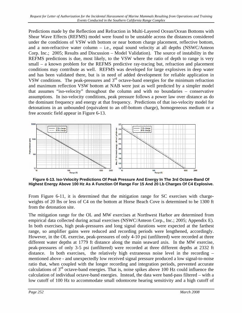
Request for Letter of Authorization for the Incidental Harassment of Marine Mammals Resulting from Operations and Training Events Conducted in the Southern California Range Complex
Page 252 March 2008
Predictions made by the Reflection and Refraction in Multi-Layered Ocean/Ocean Bottoms with Shear Wave Effects (REFMS) model were found to be unstable across the distances considered under the conditions of VSW with bottom or near bottom charge placement, reflective bottom, and a non-refractive water column – i.e., equal sound velocity at all depths (NSWC/Anteon Corp. Inc.; 2005; Results and Discussion – Model Validation). The source of instability in the REFMS predictions is due, most likely, to the VSW where the ratio of depth to range is very small – a known problem for the REFMS predictive ray-tracing but, refraction and placement conditions may contribute as well. REFMS was developed for large explosives in deep water and has been validated there, but is in need of added development for reliable application in VSW conditions. The peak-pressures and 3rd octave-band energies for the minimum refraction and maximum reflection VSW bottom at NAB were just as well predicted by a simpler model that assumes “iso-velocity” throughout the column and with no boundaries – conservative assumptions. In iso-velocity conditions, peak pressure follows a power law over distance as do the dominant frequency and energy at that frequency. Predictions of that iso-velocity model for detonations in an unbounded (equivalent to an off-bottom charge), homogeneous medium or a free acoustic field appear in Figure 6-13.
Figure 6-13. Iso-Velocity Predictions Of Peak Pressure And Energy In The 3rd Octave-Band Of
Highest Energy Above 100 Hz As A Function Of Range For 15 And 20 Lb Charges Of C4 Explosive.
From Figure 6-11, it is determined that the mitigation range for SC exercises with charge-weights of 20 lbs or less of C4 on the bottom at Horse Beach Cove is determined to be 1300 ft from the detonation site.
The mitigation range for the OL and MW exercises at Northwest Harbor are determined from empirical data collected during actual exercises (NSWC/Anteon Corp., Inc.; 2005; Appendix E). In both exercises, high peak-pressures and long signal durations were expected at the farthest range, so amplifier gains were reduced and recording periods were lengthened, accordingly. However, in the OL exercise, peak-pressures of only 4-10 psi (unfiltered) were recorded at three different water depths at 1779 ft distance along the main seaward axis. In the MW exercise, peak-pressures of only 3-5 psi (unfiltered) were recorded at three different depths at 2332 ft distance. In both exercises, the relatively high extraneous noise level in the recording – mentioned above - and unexpectedly low received signal pressure produced a low signal-to-noise ratio that, when coupled with the longer recording and integration periods, prevented accurate calculations of 3rd octave-band energies. That is, noise spikes above 100 Hz could influence the calculation of individual octave-band energies. Instead, the data were band-pass filtered – with a low cutoff of 100 Hz to accommodate small odontocete hearing sensitivity and a high cutoff of

Request for Letter of Authorization for the Incidental Harassment of Marine Mammals Resulting from Operations and Training Events Conducted in the Southern California Range Complex
March 2008 Page 253
40 KHz to remove extraneous noise above that frequency – and total energies, instead of 3rd octave-band energies, were reported. Thus, in the OL exercise, total energies of 181-187 dB re 1 µPa2 ·sec were recorded at the three different water depths at 1779 ft distance. In the MW exercise, total energies of 180-185 dB re 1 µPa2 ·sec were recorded at different depths at 2332 ft distance.
In addition to energy in the water, these total energy values incorporate some noise that remained in the pass-band after filtering. These totals can be related to maximum 3rd octave-band energies by comparison with results obtained in the SC exercises. In two SC exercises with bottom charges, one at NAB and one at Northwest Harbor, the total energy and the energy in the 3rd octave band of highest energy were considered for each pressure gage in both exercises. The mean difference, across all gages, between total energy and maximum 3rd octave-band energy was 6.6 dB with a standard deviation of 2.0 dB. That is, the total energies given above indicate that the probable maximum 3rd octave band energy was at or below the onset-TTS energy criterion at 1780 ft distance in the OL exercise and below that criterion at 2332 ft distance for the MW exercise. Considering the added noise, the actual energies – total and probable maximum 3rd octave-band - were somewhat less. Thus, it is determined that the mitigation range for OL and MW exercises with charge-types and charge-weights described at Northwest Harbor is determined to be 2000 ft from the detonation site.
The total energy values, described above for these exercises, are not comparable with recently suggested revisions to the impulse criteria for onset-TTS resulting from exposure to very large single charges in very deep water. That suggested criterion uses a peak-pressure of 23 psi as a “limiting” value and 183 dB re 1 µPa2 ·sec received, C-weighted energy flux density level. C-weighting has somewhat different filter characteristics than band-pass filtering and, for “mid-frequency” cetacea, the C-weighting has low and high-frequency cutoffs of 150 Hz and 160 KHz. For perspective, a mid-depth pressure gage at 1779 ft distance in the OL exercise recorded 9 psi peak-pressure and 187 dB re 1 µPa2 ·sec total energy with 100 Hz and 40 KHz band-pass filtering. Using band-pass filtering between 150 Hz and 40 KHz as a conservative approximation to mid-frequency C-weighting – with 40 KHz used to remove high frequency noise as before - that gage’s total energy at 1780 ft distance would be 183 dB re 1 µPa2 ·sec. That value would include additional noise in the pass-band as before. Beyond that perspective, there are substantial differences between the very deep water, large charge scenario of the suggested revised criteria and the present one with its single and multiple relatively small explosives laid on the bottom in very shallow water. Different blast conditions, configurations, and charge-weight produce substantially different waveforms at a distance and therefore, likely differ considerably in their effects on auditory tissue. For these reasons, the previously described dual-criterion is used in this LOA. It is the dual-criterion previously used in DoN (2001) and approved in CFR (2001).
6.18 Modeling Acoustic and Explosive Effects The methodology for analyzing potential impacts from sonar and explosives is presented in in this section, which defines the model process in detail, describes how the impact threshold derived from Navy-NMFS consultations are derived, and discusses relative potential impact based on species biology.
The Navy acoustic exposure model process uses a number of inter-related software tools to assess potential exposure of marine mammals to Navy generated underwater sound including

Request for Letter of Authorization for the Incidental Harassment of Marine Mammals Resulting from Operations and Training Events Conducted in the Southern California Range Complex
Page 254 March 2008
sonar and explosions. For sonar, these tools estimate potential impact volumes and areas over a range of thresholds for sonar specific operating modes. Results are based upon extensive pre-computations over the range of acoustic environments that might be encountered in the operating area.
The process includes four steps used to calculate potential exposures:
• Identify unique acoustic environments that encompass the operating area. Parameters include depth and seafloor geography, bottom characteristics and sediment type, wind and surface roughness, sound velocity profile, surface duct, sound channel, and convergence zones.
• Compute transmission loss (TL) data appropriate for each sensor type in each of these acoustic environments. Propagation can be complex depending on a number of environmental parameters listed in step one, as well as sonar operating parameters such as directivity, source level, ping rate, and ping length, and for explosives the amount of explosive material detonated. The Navy standard CASS-GRAB acoustic propagation model is used to resolve these complexities for underwater propagation prediction.
• Use that TL to estimate the total sound energy received at each point in the acoustic environment.
• Apply this energy to predicted animal density for that area to estimate potential acoustic exposure, with animals distributed in 3-D based on best available science on animal dive profiles.
• Modeling of the effects of mid-frequency sonar and underwater detonations was conducted using methods described in the following sections.
The primary potential impact to marine mammals from underwater acoustics is Level B harassment from noise. For explosions, in the absence of any mitigation or monitoring measures, there is a very small chance that a marine mammal could be injured or killed when exposed to the energy generated from an explosive force on the sea floor. Analysis of noise impacts to cetaceans is based on criteria and thresholds initially presented in U.S. Navy Environmental Impact Statements for ship shock trials of the Seawolf submarine and the Winston Churchill (DDG 81), and subsequently adopted by NMFS.
Non-lethal injurious impacts (Level A Harassment) are defined in those documents as tympanic membrane (TM) rupture and the onset of slight lung injury. The threshold for Level A Harassment corresponds to a 50-percent rate of TM rupture, which can be stated in terms of an energy flux density (EFD) value of 205 dB re 1 µPa2-s. TM rupture is well-correlated with permanent hearing impairment. Ketten (1998) indicates a 30-percent incidence of permanent threshold shift (PTS) at the same threshold.
The criteria for onset of slight lung injury were established using partial impulse because the impulse of an underwater blast wave was the parameter that governed damage during a study using mammals, not peak pressure or energy (Yelverton 1981). Goertner (1982) determined a way to calculate impulse values for injury at greater depths, known as the Goertner "modified" impulse pressure. Those values are valid only near the surface because as hydrostatic pressure

Request for Letter of Authorization for the Incidental Harassment of Marine Mammals Resulting from Operations and Training Events Conducted in the Southern California Range Complex
March 2008 Page 255
increases with depth, organs like the lung, filled with air, compress. Therefore the "modified" impulse pressure thresholds vary from the shallow depth starting point as a function of depth.
The shallow depth starting points for calculation of the "modified" impulse pressures are mass-dependent values derived from empirical data for underwater blast injury (Yelverton 1981). During the calculations, the lowest impulse and body mass for which slight, and then extensive, lung injury found during a previous study (Yelverton et al 1973) were used to determine the positive impulse that may cause lung injury. The Goertner model is sensitive to mammal weight; such that smaller masses have lower thresholds for positive impulse so injury and harassment will be predicted at greater distances from the source for them. Impulse thresholds of 13.0 and 31.0 psi-msec, found to cause slight and extensive injury in a dolphin calf, were used as thresholds in the analysis contained in this document.
Level B (non-injurious) Harassment includes temporary (auditory) threshold shift (TTS), a slight, recoverable loss of hearing sensitivity. One criterion used for TTS is 182 dB re 1 µPa2-s maximum EFD level in any 1/3-octave band above 100 Hz for toothed whales (e.g., dolphins). A second criterion, 23 psi, has recently been established by NMFS to provide a more conservative range for TTS when the explosive or animal approaches the sea surface, in which case explosive energy is reduced, but the peak pressure is 1 µPa2-s is not. NMFS applies the more conservative of these two. Table 6-4 lists the thresholds for explosives.
Table 6-4. Explosive Source Thresholds
Threshold Type (Explosives) Threshold Level Level A – 50% Eardrum rupture (peak one-third octave energy) 205 dB
Temporary Threshold Shift (TTS) (peak one-third octave energy) 182 dB Temporary Threshold Shift (TTS) (peak pressure) 23 psi
Level A – Slight lung injury (positive impulse) 13 psi-ms Fatality – 1% Mortal lung injury (positive impulse) 31 psi-ms
For non-explosive sound sources, Level B Harassment includes behavioral modifications resulting from repeated noise exposures (below TTS) to the same animals over a relatively short period of time. Cetaceans exposed to ELs of 195 dB re 1 µPa2-s up to 215 dB re 1 µPa2-s are assumed to experience TTS. At 215 dB re 1 µPa2-s, cetaceans are assumed to experience PTS. Unlike cetaceans, the TTS and PTS thresholds used for pinnipeds vary with species. Otariids have thresholds of 206 dB re 1 µPa2-s for TTS and 226 dB re 1 µPa2-s for PTS. Northern elephant seals are similar to otariids (TTS = 204 dB re 1 µPa2-s, PTS = 224 dB re 1 µPa2-s) but are lower for harbor seals (TTS = 183 dB re 1 µPa2-s, PTS = 203 dB re 1 µPa2-s).
A certain proportion of marine mammals are expected to experience behavioral disturbance at different received sound pressure levels and are counted as Level B harassment exposures. The details of this “sub-TTS” theory and calculation are described in the later in this section. Table 6-5 lists the physiological thresholds for sonar derived from NMFS consultations and rulemaking.
The sound sources will be located in an area that is inhabited by species listed as threatened or endangered under the Endangered Species Act (ESA, 16 USC §§ 1531-1543). If a federal agency determines that its proposed action “may affect” a listed species, it is required to consult, either formally or informally, with the appropriate regulator. The Navy will initiate formal consultation

Request for Letter of Authorization for the Incidental Harassment of Marine Mammals Resulting from Operations and Training Events Conducted in the Southern California Range Complex
Page 256 March 2008
under the ESA by submitting a Biological Assessment to NMFS, detailing the proposed action’s potential effects on listed species and any designated critical habitat.
6.18.1 Acoustic Sources The Southern California (SOCAL) acoustic sources are categorized as either broadband (producing sound over a wide frequency band) or narrowband (producing sound over a frequency band that that is small in comparison to the center frequency). In general, the narrowband sources in this exercise are ASW sonars and the broadband sources are explosives. This delineation of source types has a couple of implications. First, the transmission loss used to determine the impact ranges of narrowband ASW sonars can be adequately characterized by model estimates at a single frequency. Broadband explosives, on the other hand, produce significant acoustic energy across several frequency decades of bandwidth. Propagation loss is sufficiently sensitive to frequency as to require model estimates at several frequencies over such a wide band.
Second, the types of sources have different sets of harassment metrics and thresholds. Energy metrics are defined for both types. However, explosives are impulsive sources that produce a shock wave that dictates additional pressure-related metrics (peak pressure and positive impulse). Detailed descriptions of both types of sources are provided in the following subsections.
6.18.2 Sonars To estimate impacts from mid- and high-frequency sonar, five types of narrowband sonars representative of those used in operations in the SOCAL Range Complex were modeled. Exposure estimates are calculated for each sonar according to the manner in which it operates. For example, the SQS-53C is a hull-mounted, surface ship sonar that operates for many hours at a time, so it is most useful to calculate and report SQS-53C exposures per hour of operation. The SQS-56C is a hull-mounted, surface ship sonar (not as powerfull as the SQS-53C) that operates for many hours at a time, so it is most useful to calculate and report SQS-56C exposures per hour of operation. The AQS-22 is a helicopter-deployed sonar, which is lowered into the water, pings a number of times, and then moves to a new location. For the AQS-22, it is most helpful to calculate and report exposures per dip. Table 6-5 presents the deploying platform, frequency class, and the reporting metric for each sonar.
Table 6-5. Active Sonars Employed in SOCAL Range
Sonar Description Frequency Class Exposures Reported
MK-48 Torpedo sonar High frequency Per torpedo AN/SQS-53C Surface ship sonar Mid-frequency Per hour AN/SQS-56C Surface ship sonar Mid-frequency Per hour AN/SSQ-62 Sonobuoy sonar Mid-frequency Per sonobuoy AN/AQS-22 Helicopter-dipping sonar Mid-frequency Per dip
Note that MK-48 source described here is the active pinger on the torpedo; the explosive source of the detonating torpedo is described in the next subsection.
The acoustic modeling that is necessary to support the exposure estimates for each of these sonars relies upon a generalized description of the manner of the sonar’s operating modes. This description includes the following:

Request for Letter of Authorization for the Incidental Harassment of Marine Mammals Resulting from Operations and Training Events Conducted in the Southern California Range Complex
March 2008 Page 257
• “Effective” energy source level – The total energy across the band of the source, scaled by the pulse length (10 log10 [pulse length]), and corrected for source beam width so that it reflects the energy in the direction of the main lobe. The beam pattern correction consists of two terms:
• Horizontal directivity correction: 10 log10 (360 / horizontal beam width)
• Vertical directivity correction: 10 log10 (2 / [sin(θ1) – sin(θ2)]), where θ1 and θ2 are the 3-dB down points on the main lobe.
• Source depth – Depth of the source in meters.
• Nominal frequency – Typically the center band of the source emission. These are frequencies that have been reported in open literature and are used to avoid classification issues. Differences between these nominal values and actual source frequencies are small enough to be of little consequence to the output impact volumes.
• Source directivity – The source beam is modeled as the product of a horizontal beam pattern and a vertical beam pattern. Two parameters define the horizontal beam pattern:
• Horizontal beam width – Width of the source beam (degrees) in the horizontal plane (assumed constant for all horizontal steer directions).
• Horizontal steer direction – Direction in the horizontal in which the beam is steered relative to the direction in which the platform is heading
The horizontal beam is rectangular with constant response across the width of the beam and with flat, 20-dB down sidelobes. (Note that steer directions φ, –φ, 180o – φ, and 180o + φ all produce equal impact volumes.)
Similarly, two parameters define the vertical beam pattern:
• Vertical beam width – Width of the source beam (degrees) in the vertical plane measured at the 3-dB down point. (The width is that of the beam steered towards broadside and not the width of the beam at the specified vertical steer direction.)
• Vertical steer direction – Direction in the vertical plane that the beam is steered relative to the horizontal (upward looking angles are positive).
To avoid sharp transitions that a rectangular beam might introduce, the power response at vertical angle θ is
max { sin2 [ n(θs – θ) ] / [ n sin (θs – θ) ]2, 0.01 }
where n = 180o / θw is the number of half-wavelength-spaced elements in a line array that produces a main lobe with a beam width of θw. θs is the vertical beam steer direction.
Ping spacing – Distance between pings. For most sources this is generally just the product of the speed of advance of the platform and the repetition rate of the sonar. Animal motion is generally of no consequence as long as the source motion is greater than the speed of the animal (nominally, three knots). For stationary (or nearly stationary) sources, the “average” speed of the

Request for Letter of Authorization for the Incidental Harassment of Marine Mammals Resulting from Operations and Training Events Conducted in the Southern California Range Complex
Page 258 March 2008
animal is used in place of the platform speed. The attendant assumption is that the animals are all moving in the same constant direction.
These parameters are defined for each of the active sonars (including two operating modes for the 53C) in Table 6-6.
Table 6-6. Source Description of SOCAL Mid- and High-Frequency Active Sonars
Sonar Source Depth
Center Freq
Source Level
Emission Spacing
Vertical Directivity
Horizontal Directivity
MK-48 27 m > 10 kHz Classified 144 m Omni Omni AN/SQS-53C Search Mode 7 m 3.5 kHz 235 dB 154 m Omni 240o Forward-
looking AN/SQS-53C
Kingfisher Mode 7 m 3.5 kHz 236 dB 4.6 m 20o Width 42o D/E
120o Forward-looking
AN/SQS-56C 7 m 6.8 to 8.2 kHz 223 dB
AN/SSQ-62 27 m 8 kHz 201 dB 450 m Omni Omni AN/AQS-22 27 m 4.1 kHz 217 dB 15 m Omni Omni
6.18.3 Explosives Explosives detonated underwater introduce loud, impulsive, broadband sounds into the marine environment. Three source parameters influence the effect of an explosive: the weight of the explosive warhead, the type of explosive material, and the detonation depth. The net explosive weight (or NEW) accounts for the first two parameters. The NEW of an explosive is the weight of only the explosive material in a given round, referenced to the explosive power of TNT.
The detonation depth of an explosive is particularly important due to a propagation effect known as surface-image interference increasingly. For sources located near the sea surface, a distinct interference pattern arises from the coherent sum of the two paths that differ only by a single reflection from the pressure-release surface. As the source depth and/or the source frequency decreases, these two paths increasingly, destructively interfere with each other, reaching total cancellation at the surface (barring surface-reflection scattering loss). For the SOCAL Range there are two types of explosive sources: demolition charges and munitions (Mk-48 torpedo, Maverick and Harpoon missiles, Mk-82 and Mk-83 bombs, 5” rounds and 76 mm rounds). Demolition charges are typically modeled as detonating near the middle of the water column. The Mk-48 detonates immediately below the hull of its target (nominally 50 feet). A source depth of two meters is used for bombs and missiles that do not strike their target. For the gunnery rounds, a source depth of one foot is used. The NEW for these sources are as follows:
• Demolition charge – 20 pounds, • Mk-48 – 851 pounds, • Maverick – 78.5 pounds, • Harpoon – 448 pounds, • Mk-82 – 238 pounds, • Mk-83 – 574 pounds, • 5” rounds – 9.54 pounds, and • 76 mm rounds – 1.6 pounds.

Request for Letter of Authorization for the Incidental Harassment of Marine Mammals Resulting from Operations and Training Events Conducted in the Southern California Range Complex
March 2008 Page 259
The exposures expected to result from these sources are computed on a per in-water explosive basis. The cumulative effect of a series of explosives can often be derived by simple addition if the detonations are spaced widely in time or space, allowing for sufficient animal movements as to ensure a different population of animals is considered for each detonation.
The cases in which simple addition of the exposures estimates may not be appropriate are addressed by the modeling of a “representative” sinking exercise (SINKEX). In a SINKEX, a decommissioned surface ship is towed to a specified deep-water location and there used as a target for a variety of weapons. Although no two SINKEXs are ever the same, a representative case derived from past exercises is described in the Programmatic SINKEX Overseas Environmental Assessment (March 2006) for the Western North Atlantic.
In a SINKEX, weapons are typically fired in order of decreasing range from the source with weapons fired until the target is sunk. A torpedo is used after all munitions have been expended if the target is still afloat. Since the target may sink at any time during the exercise, the actual number of weapons used can vary widely. In the representative case, however, all of the ordnances are assumed expended; this represents the worst case of maximum exposure.
The sequence of weapons firing for the representative SINKEX is described in Table 6-7. Guided weapons are nearly 100% accurate and are modeled as hitting the target (that is, no underwater acoustic effect) in all but two cases: (1) the Maverick is modeled as a miss to represent the occasional miss, and (2) the MK-48 torpedo intentionally detonates in the water column immediately below the hull of the target. Unguided weapons are more frequently off-target and are modeled according to the statistical hit/miss ratios. Note that these hit/miss ratios are artificially low in order to demonstrate a worst-case scenario; they should not be taken as indicative of weapon or platform reliability.
Table 6-7. Representative SINKEX Weapons Firing Sequence
Time (Local) Event Description
0900 Range Control Officer receives reports that the exercise area is clear of non-participant ship traffic, marine mammals, and sea turtles.
0909 Hellfire missile fired, hits target. 0915 2 HARM missiles fired, both hit target (5 minutes apart). 0930 1 Penguin missile fired, hits target. 0940 3 Maverick missiles fired, 2 hit target, 1 misses (5 minutes apart). 1145 1 SM-1 fired, hits target. 1147 1 SM-2 fired, hits target. 1205 5 Harpoon missiles fired, all hit target (1 minute apart). 1300-1335
7 live and 3 inert MK 82 bombs dropped – 7 hit target, 2 live and 1 inert miss target (4 minutes apart).
1355-1410 4 MK 83 bombs dropped – 3 hit target, 1 misses target (5 minutes apart).
1500 Surface gunfire commences – 400 5-inch rounds fired (one every 6 seconds), 280 hit target, 120 miss target.
1700 MK 48 Torpedo fired, hits, and sinks target.

Request for Letter of Authorization for the Incidental Harassment of Marine Mammals Resulting from Operations and Training Events Conducted in the Southern California Range Complex
Page 260 March 2008
6.19 Environmental Provinces Propagation loss ultimately determines the extent of the Zone of Influence (ZOI) for a particular source activity. In turn, propagation loss as a function of range responds to a number of environmental parameters:
• water depth
• sound speed variability throughout the water column
• bottom geo-acoustic properties, and
• wind speed
Due to the importance that propagation loss plays in Anti-Submarine Warfare (ASW), the Navy has over the last four to five decades invested heavily in measuring and modeling these environmental parameters. The result of this effort is the following collection of global databases of these environmental parameters, most of which are accepted as standards for all Navy modeling efforts.
• Water depth – Digital Bathymetry Data Base Variable Resolution (DBDBV)
• Sound speed – Generalized Digital Environmental Model (GDEM)
• Bottom loss – Low-Frequency Bottom Loss (LFBL), Sediment Thickness Database, and High-Frequency Bottom Loss (HFBL), and
• Wind speed – U.S. Navy Marine Climatic Atlas of the World
This section provides a discussion of the relative impact of these various environmental parameters. These examples then are used as guidance for determining environmental provinces (that is, regions in which the environmental parameters are relatively homogenous and can be represented by a single set of environmental parameters) within the SOCAL Range.
Impact of Environmental Parameters Within a typical operating area, the environmental parameter that tends to vary the most is bathymetry. It is not unusual for water depths to vary by an order of magnitude or more, resulting in significant impacts upon the Zone of Influence (ZOI) calculations. Bottom loss can also vary considerably over typical operating areas but its impact upon ZOI calculations tends to be limited to waters on the continental shelf and the upper portion of the slope. Generally, the primary propagation paths in deep water, from the source to most of the ZOI volume, do not involve any interaction with bottom. In shallow water, particularly if the sound velocity profile directs all propagation paths to interact with the bottom, bottom loss variability can play a larger role.
The spatial variability of the sound speed field is generally small over operating areas of typical size. The presence of a strong oceanographic front is a noteworthy exception to this rule. To a lesser extent, variability in the depth and strength of a surface duct can be of some importance. In the mid-latitudes, seasonal variation often provides the most significant variation in the sound speed field. For this reason, both summer and winter profiles are modeled for each selected environment.

Request for Letter of Authorization for the Incidental Harassment of Marine Mammals Resulting from Operations and Training Events Conducted in the Southern California Range Complex
March 2008 Page 261
6.19.1 Environmental Provincing Methodology The underwater acoustic environment can be quite variable over ranges in excess of ten kilometers. For ASW applications, ranges of interest are often sufficiently large as to warrant the modeling of the spatial variability of the environment. In the propagation loss calculations, each of the environmental parameters is allowed to vary (either continuously or discretely) along the path from acoustic source to receiver. In such applications, each propagation loss calculation is conditioned upon the particular locations of the source and receiver.
On the other hand, the range of interest for marine animal harassment by most Naval activities is more limited. This reduces the importance of the exact location of source and marine animal and makes the modeling required more manageable in scope.
In lieu of trying to model every environmental profile that can be encountered in an operating area, this effort utilizes a limited set of representative environments. Each environment is characterized by a fixed water depth, sound velocity profile, and bottom loss type. The operating area is then partitioned into homogeneous regions (or provinces) and the most appropriately representative environment is assigned to each. This process is aided by some initial provincing of the individual environmental parameters. The Navy-standard high-frequency bottom loss database in its native form is globally partitioned into nine classes. Low-frequency bottom loss is likewise provinced in its native form, although it is not considered in the process of selecting environmental provinces. Only the broadband sources produce acoustic energy at the frequencies of interest for low-frequency bottom loss (typically less than 1 kHz); even for those sources the low-frequency acoustic energy is secondary to the energy above 1 kHz. The Navy-standard sound velocity profiles database is also available as a provinced subset. Only the Navy-standard bathymetry database varies continuously over the world’s oceans. However, even this environmental parameter is easily provinced by selecting a finite set of water depth intervals. For this analysis “octave-spaced” intervals (10, 20, 50, 100, 200, 500, 1000, 2000, and 5000 m) provide an adequate sampling of water depth dependence.
Zone of influence volumes are then computed using propagation loss estimates derived for the representative environments. Finally, a weighted average of the ZOI volumes is taken over all representative environments; the weighting factor is proportional to the geographic area spanned by the environmental province.
The selection of representative environments is subjective. However, the uncertainty introduced by this subjectivity can be mitigated by selecting more environments and by selecting the environments that occur most frequently over the operating area of interest.
As discussed in the previous subsection, ZOI estimates are most sensitive to water depth. Unless otherwise warranted, at least one representative environment is selected in each bathymetry province. Within a bathymetry province, additional representative environments are selected as needed to meet the following requirements.
In shallow water (less than 1,000 meters), bottom interactions occur at shorter ranges and more frequently; thus significant variations in bottom loss need to be represented.
Surface ducts provide an efficient propagation channel that can greatly influence ZOI estimates. Variations in the mixed layer depth need to be accounted for if the water is deep enough to support the full extent of the surface duct.

Request for Letter of Authorization for the Incidental Harassment of Marine Mammals Resulting from Operations and Training Events Conducted in the Southern California Range Complex
Page 262 March 2008
Depending upon the size and complexity of the operating area, the number of environmental problems tends to range for 5 - 20.
6.19.2 Description of Environmental Provinces The SOCAL Range is located in an area south of 34o N, off the west coast of the US and Mexico. The range encompasses most of Warning Area W-291 and additional near-coastal areas to the north. For this analysis, eight areas within this range have been identified as representative. Seven of these areas are quasi-rectangular regions as described below and depicted in Figure 6-14.
Area 1: Immediately east of San Nicolas Island; boundary vertices are
119o 6’ W 33o 40’ N
118o 51’ W 33o 29’ N
119o 10’ W 33o 3’ N
119o 25’ W 33o 14’ N
Area 2: Between San Clemente and Santa Catalina Islands; boundary vertices are:
118o 40’ W 33o 29’ N
118o 4’ W 32o 2’ N
118o 15’ W 32o 48’ N
118o 51’ W 33o 15’ N
Area 3: Off-shore area immediately west of MCB Camp Pendleton; boundary vertices are:
117o 44’ W 33o 29’ N
117o 19’ W 33o 4’ N
117o 31’ W 32o 52’ N
117o 56’ W 33o 17’ N

Request for Letter of Authorization for the Incidental Harassment of Marine Mammals Resulting from Operations and Training Events Conducted in the Southern California Range Complex
March 2008 Page 263
Figure 6-14. Representative Areas in SOCAL Range
1
2 3
4 6
5
7

Request for Letter of Authorization for the Incidental Harassment of Marine Mammals Resulting from Operations and Training Events Conducted in the Southern California Range Complex
Page 264 March 2008
Area 4: Area immediately south and west of San Clemente Island; boundary vertices are:
118o 44’ W 33o 6’ N
118o 26’ W 32o 44’ N
119o W 32o 18’ N
119o 17’ W 32o 40’ N
Area 5: Area 25 n.m. south and east of San Clemente Island; boundary vertices are:
118o 25’ W 32o 19’ N
117o 44’ W 32o 19’ N
117o 44’ W 31o 27’ N
118o 25’ W 31o 27’ N
Area 6: Off-shore area immediately west of NB Coronado; boundary vertices are:
117o 35’ W 32o 35’ N
117o 9’ W 32o 35’ N
117o 9’ W 32o 18’ N
117o 35’ W 32o 18’ N
Area 7: Deep-water area near the middle of W-291; boundary vertices are:
119o 16’ W 30o 53’ N
118o 41’ W 30o 19’ N
119o 25’ W 29o 34’ N
120o W 30o 8’ N
The final region, Area 8, includes all areas outside the previous seven areas that are within the quasi-rectangular region bounded in latitude by 29o N and 34o N, and in longitude by 120o 30’ W and 116o 30’ W.
The acoustic sonars described in subsection 4.2 are, for the most part, deployed throughout all eight areas. The lone exception is Area 6 which is restricted to only the helicopter dipping sonar The explosive sources, other than demolition charges, are primarily limited by the SINKEX restrictions (at least 50 n.m. from land in water depths greater than 1000 fathoms) to the southern portion of Area 5, all of Area 7, and parts of Area 8. The use of demolition charges is limited to the north shore of SCI (Northwest Harbor).
This subsection describes the representative environmental provinces selected for the SOCAL Range. For all of these provinces, the average wind speed, winter and summer, is 11 knots.
The SOCAL Range contains a total of 13 distinct environmental provinces. These represent various combinations of nine bathymetry provinces, one Sound Velocity Profile (SVP) province, and three High-Frequency Bottom Loss (HFBL) classes.
The bathymetry provinces represent depths ranging from 10 meters to typical deep-water depths (slightly more than 5,000 meters). Nearly half of the range is characterized as deep-water

Request for Letter of Authorization for the Incidental Harassment of Marine Mammals Resulting from Operations and Training Events Conducted in the Southern California Range Complex
March 2008 Page 265
(depths of 2,000 meters or more). The second most prevalent water depth regime, covering more than 40% of the range, is representative of waters along the continental slope. The remaining water depths (200 meters and less) provide only small contributions (less than 10%) to the analysis. The distribution of the bathymetry provinces over the SOCAL Range is provided in Table 6-8.
Table 6-8. Distribution of Bathymetry Provinces in SOCAL Range
Province Depth (m) Frequency of Occurrence 10 Demolition Charges Only 20 0.33 % 50 1.17 %
100 1.74 % 200 3.28 % 500 9.92 % 1000 33.66 % 2000 17.03 % 5000 32.54 %
A single SVP province (45) describes the entire SOCAL Range. The seasonal variation is likewise of limited dynamic range, as might be expect given that the range is located in temperate waters. The surface sound speed of the winter profile is about ten m/s slower than the summer profile as depicted in Figure 6-15. Both seasons exhibit a shallow and relatively weak surface duct.
0200
400600
8001000
1475 1485 1495 1505 1515 1525
Sound Speed (m/s)
Dep
th (m
)
WinterSummer
Figure 6-15. Winter and Summer SVPs in SOCAL Range
The three HFBL classes represented in the SOCAL Range are either low-loss bottoms (class 2, typically in shallow water) or high-loss bottoms (classes 7 or 8, predominately in intermediate to deep water). This partitioning by water depth leads to a distribution that is more than 90 % high-loss bottoms as indicated in Table 6-9.

Request for Letter of Authorization for the Incidental Harassment of Marine Mammals Resulting from Operations and Training Events Conducted in the Southern California Range Complex
Page 266 March 2008
Table 6-9. Distribution of High-Frequency Bottom Loss Classes in SOCAL Range
HFBL Class Frequency of Occurrence 2 6.22 % 7 16.65 % 8 77.13 %
The logic for consolidating the environmental provinces focuses upon water depth, using the sound speed profile (in deep water) and the HFBL class (in shallow water) as secondary differentiating factors. The first consideration was to ensure that all six bathymetry provinces are represented. Then within each bathymetry province further partitioning of provinces proceeded as follows:
The three shallowest bathymetry provinces are each represented by one environmental province. In each case, the bathymetry province is dominated (in some cases almost exclusively) by a single HFBL class, so that the secondary differentiating environmental parameter is of no consequence.
The 100-, 200-, and 500-meter bathymetry provinces each have two environmental provinces, differing in HFBL class only (one has a low-loss bottom, the other a high-loss bottom). Since the frequency of occurrence of the secondary province is not overwhelmed by the dominant province, both are included in the analysis to ensure thoroughness.
The 1000- and 2000-meter bathymetry provinces each contain two environmental provinces that feature different HFBL classes. However, in both cases the dominant province in the pair occurs more than a hundred times more frequently rendering the secondary province of no consequence in this analysis.
The 5000-meter bathymetry province consists of three environmental provinces that differ only in HFBL class. One of the three provinces occurs so infrequently in comparison to the other two that it is excluded from this analysis.
The resulting thirteen environmental provinces used in the SOCAL Range acoustic modeling are described in Tables 6-10 and 6-11.

Request for Letter of Authorization for the Incidental Harassment of Marine Mammals Resulting from Operations and Training Events Conducted in the Southern California Range Complex
March 2008 Page 267
Table 6-10. Distribution of Environmental Provinces in SOCAL Range
Environmental Province
Water Depth
SVP Province
HFBL Class
LFBL Provinc
e
Sediment Thickness
Frequency of Occurrence
1 20 m 45 2 0 0.2 secs 0.44 % 2 50 m 45 2 0 0.2 secs 1.05 % 3 100 m 45 2 0 0.2 secs 1.13 % 4 200 m 45 2 0 0.2 secs 0.90 % 5 200 m 45 8 – 49* 0.2 secs 0.66 % 6 500 m 45 2 0 0.2 secs 1.02 % 7 500 m 45 8 – 49* 0.2 secs 6.06 % 8 1000 m 45 8 – 49* 0.2 secs 22.34 % 9 2000 m 45 8 13 0.18 secs 27.58 %
10 5000 m 45 7 13 0.11 secs 24.40 % 11 5000 m 45 8 13 0.11 secs 13.66 % 12 100 m 45 8 – 49* 0.2 secs 0.36 % 13 10 m 45 2 0 0.2 secs Demolition Charges
Only
* Negative province numbers indicate shallow water provinces
The percentages given in the preceding table indicate the frequency of occurrence of each environmental province across all eight areas in the SOCAL Range as described in Figure 6-10. The distribution of the environments within each of the eight individual areas in provided in Table 6-11.
Table 6-11. Distribution of Environmental Provinces within SOCAL Areas
Environmental Province Area 1 Area 2 Area 3 Area 4 Area 5 Area 6 Area 7 Area 8
1 1.33% 1.00% 0.00% 0.09% 0.00% 7.44% 0.00% 0.45% 2 3.55% 2.19% 0.84% 1.54% 0.00% 7.89% 0.00% 1.05% 3 0.00% 0.66% 2.95% 1.30% 0.00% 4.57% 0.00% 1.13% 4 0.00% 0.80% 4.70% 5.37% 0.00% 4.49% 0.00% 0.90% 5 14.58% 2.73% 1.15% 4.71% 0.18% 1.07% 0.00% 0.66% 6 0.00% 2.69% 10.06% 5.10% 0.00% 2.27% 0.00% 1.02% 7 31.20% 10.87% 43.13% 13.20% 3.53% 15.44% 0.00% 6.06% 8 37.23% 54.90% 36.69% 51.81% 43.57% 48.97% 0.00% 22.34% 9 6.45% 21.64% 0.00% 12.62% 52.72% 7.86% 6.82% 27.58%
10 0.00% 0.00% 0.00% 0.00% 0.00% 0.00% 47.68% 24.40% 11 0.00% 0.00% 0.00% 0.00% 0.00% 0.00% 45.50% 13.66% 12 5.66% 2.52% 0.48% 4.26% 0.00% 0.00% 0.00% 0.36% 13 0.00% 0.00% 0.00% 0.00% 0.00% 0.00% 0.00% 0.39%
Finally, the SINKEX areas are limited to regions that are more than 50 n.m. from land and deeper than 1000 fathoms. This includes part of Area 5, all of Area 7 and part of Area 8. The distribution of environmental provinces in these three areas is provided in Table 6-12.

Request for Letter of Authorization for the Incidental Harassment of Marine Mammals Resulting from Operations and Training Events Conducted in the Southern California Range Complex
Page 268 March 2008
Table 6-12. Distribution of Environmental Provinces within SINKEX Areas
Environmental Province Area 5 Area 7 Area 8 All Areas 9 100.00 % 6.82 % 29.74 % 26.53 %
10 0.00 % 47.68 % 42.17 % 43.10 % 11 0.00 % 45.50 % 28.09 % 30.37 %
6.20 Impact Volumes and Impact Ranges Many naval actions include the potential to injure or harass marine animals in the neighboring waters through noise emissions. The number of animals exposed to potential harassment in any such action is dictated by the propagation field and the characteristics of the noise source.
The impact volume associated with a particular activity is defined as the volume of water in which some acoustic metric exceeds a specified threshold. The product of this impact volume with a volumetric animal density yields the expected value of the number of animals exposed to that acoustic metric at a level that exceeds the threshold. The acoustic metric can either be an energy term (energy flux density, either in a limited frequency band or across the full band) or a pressure term (such as peak pressure or positive impulse). The thresholds associated with each of these metrics define the levels at which half of the animals exposed will experience some degree of harassment (ranging from behavioral change to mortality).
Impact volume is particularly relevant when trying to estimate the effect of repeated source emissions separated in either time or space. Impact range, which is defined as the maximum range at which a particular threshold is exceeded for a single source emission, defines the range to which marine mammal activity is monitored in order to meet mitigation requirements.
With the exception of explosive sources, the sole relevant measure of potential harm to the marine wildlife due to sonar operations is the accumulated (summed over all source emissions) energy flux density received by the animal over the duration of the activity. Harassment measures for explosive sources include energy flux density and pressure-related metrics (peak pressure and positive impulse). Regardless of the type of source, estimating the number of animals that may be injured or otherwise harassed in a particular environment entails the following steps.
Each source emission is modeled according to the particular operating mode of the sonar. The “effective” energy source level is computed by integrating over the bandwidth of the source, scaling by the pulse length, and adjusting for gains due to source directivity. The location of the source at the time of each emission must also be specified.
For the relevant environmental acoustic parameters, transmission loss (TL) estimates are computed, sampling the water column over the appropriate depth and range intervals. TL data are sampled at the typical depth(s) of the source and at the nominal center frequency of the source. If the source is relatively broadband, an average over several frequency samples is required.
The accumulated energy within the waters that the source is “operating” is sampled over a volumetric grid. At each grid point, the received energy from each source emission is modeled as the effective energy source level reduced by the appropriate propagation loss from the location of the source at the time of the emission to that grid point and summed. For the peak pressure or positive impulse, the appropriate metric is similarly modeled for each emission. The maximum value of that metric, over all emissions, is stored at each grid point.

Request for Letter of Authorization for the Incidental Harassment of Marine Mammals Resulting from Operations and Training Events Conducted in the Southern California Range Complex
March 2008 Page 269
The impact volume for a given threshold is estimated by summing the incremental volumes represented by each grid point for which the appropriate metric exceeds that threshold.
Finally, the number of exposures is estimated as the “product” (scalar or vector, depending upon whether an animal density depth profile is available) of the impact volume and the animal densities.
This section describes in detail the process of computing impact volumes (that is, the first four steps described above). This discussion is presented in two parts: active sonars and explosive sources. The relevant assumptions associated with this approach and the limitations that are implied are also presented. The final step, is the computation of the number of exposures.
6.20.1 Computing Impact Volumes for Active Sonars This section provides a detailed description of the approach taken to compute impact volumes for active sonars. Included in this discussion are:
• Identification of the underwater propagation model used to compute transmission loss data, a listing of the source-related inputs to that model, and a description of the output parameters that are passed to the energy accumulation algorithm.
• Definitions of the parameters describing each sonar type.
• Description of the algorithms and sampling rates associated with the energy accumulation algorithm.
Transmission Loss Calculations Transmission loss (TL) data are pre-computed for each of two seasons in each of the environmental provinces described in the previous subsection using the GRAB propagation loss model (Keenan, 2000). The TL output consists of a parametric description of each significant eigenray (or propagation path) from source to animal. The description of each eigenray includes the departure angle from the source (used to model the source vertical directivity later in this process), the propagation time from the source to the animal (used to make corrections to absorption loss for minor differences in frequency and to incorporate a surface-image interference correction at low frequencies), and the transmission loss suffered along the eigenray path.
The frequency and source depth TL inputs are specified in Table 6-13. Table 6-13. TL Frequency and Source Depth by Sonar Type
Sonar Frequency Source Depth MK-48 > 10 kHz 27 m
AN/SQS-53C 3.5 kHz 7 m AN/SQS-56C 6.8 to 8.2 kHz 7 m AN/AQS-22 4.1 kHz 27 m AN/ASQ-62 8 kHz 27 m
The eigenray data for a single GRAB model run are sampled at uniform increments in range out to a maximum range for a specific “animal” (or “target” in GRAB terminology) depth. Multiple GRAB runs are made to sample the animal depth dependence. The depth and range sampling

Request for Letter of Authorization for the Incidental Harassment of Marine Mammals Resulting from Operations and Training Events Conducted in the Southern California Range Complex
Page 270 March 2008
parameters are summarized in Table 6-14. Note that some of the low-power sources do not require TL data to large maximum ranges.
Table 6-14. TL Depth and Model Range Sampling Parameters by Sonar Type
Sonar Range Step Maximum Range * Animal Depth MK-48 10 m 10 km 0 – 1 km in 5 m steps
1 km – Bottom in 10 m steps
AN/SQS-53C 10 m 200 km 0 – 1 km in 5 m steps 1 km – Bottom in 10 m steps
AN/AQS-22 10 m 10 km 0 – 1 km in 5 m steps 1 km – Bottom in 10 m steps
AN/ASQ-62 5 m 5 km 0 – 1 km in 5 m steps 1 km – Bottom in 10 m steps
* Range estimates are extent of conservative modeling assumptions and not reflective of system performance
In a few cases, most notably the AN/SQS-53C for thresholds below approximately 180 dB, TL data may be required by the energy summation algorithm at ranges greater than covered by the pre-computed GRAB data. In these cases, TL is extrapolated to the required range using a simple cylindrical spreading loss law in addition to the appropriate absorption loss. This extrapolation leads to a conservative (or under) estimate of transmission loss at the greater ranges.
Although GRAB provides the option of including the effect of source directivity in its eigenray output, this capability is not exercised. By preserving data at the eigenray level, this allows source directivity to be applied later in the process and results in fewer TL calculations.
The other important feature that storing eigenray data supports is the ability to model the effects of surface-image interference that persist over range. However, this is primarily important at frequencies lower than those associated with the sonars considered in this subsection. A detailed description of the modeling of surface-image interference is presented in the subsection on explosive sources.
Energy Summation The summation of energy flux density over multiple pings in a range-independent environment is a trivial exercise for the most part. A volumetric grid that covers the waters in and around the area of sonar operation is initialized. The source then begins its set of pings. For the first ping, the TL from the source to each grid point is determined (summing the appropriate eigenrays after they have been modified by the vertical beam pattern), the “effective” energy source level is reduced by that TL, and the result is added to the accumulated energy flux density at that grid point. After each grid point has been updated, the accumulated energy at grid points in each depth layer is compared to the specified threshold. If the accumulated energy exceeds that threshold, then the incremental volume represented by that grid point is added to the impact volume for that depth layer. Once all grid points have been processed, the resulting sum of the incremental volumes represents the impact volume for one ping.
The source is then moved along one of the axes in the horizontal plane by the specified ping separation range and the second ping is processed in a similar fashion. Again, once all grid points have been processed, the resulting sum of the incremental volumes represents the impact volume for two pings. This procedure continues until the maximum number of pings specified has been reached.

Request for Letter of Authorization for the Incidental Harassment of Marine Mammals Resulting from Operations and Training Events Conducted in the Southern California Range Complex
March 2008 Page 271
Defining the volumetric grid over which energy is accumulated is the trickiest aspect of this procedure. The volume must be large enough to contain all volumetric cells for which the accumulated energy is likely to exceed the threshold but not so large as to make the energy accumulation computationally unmanageable.
Determining the size of the volumetric grid begins with an iterative process to determine the lateral extent to be considered. Unless otherwise noted, throughout this process the source is treated as omni directional and the only animal depth that is considered is the TL target depth that is closest to the source depth (placing source and receiver at the same depth is generally an optimal TL geometry).
The first step is to determine the impact range (RMAX) for a single ping. The impact range in this case is the maximum range at which the effective energy source level reduced by the transmission loss is greater than the threshold. Next, the source is moved along a straight-line track and energy flux density is accumulated at a point that has a CPA range of RMAX at the mid-point of the source track. That total energy flux density summed over all pings is then compared to the prescribed threshold. If it is greater than the threshold (which, for the first RMAX, it must be) then RMAX is increased by ten percent, the accumulation process is repeated, and the total energy is again compared to the threshold. This continues until RMAX grows large enough to ensure that the accumulated energy flux density at that lateral range is less than the threshold. The lateral range dimension of the volumetric grid is then set at twice RMAX, with the grid centered along the source track. In the direction of advance for the source, the volumetric grid extends of the interval from [–RMAX, 3 RMAX] with the first source position located at zero in this dimension. Note that the source motion in this direction is limited to the interval [0, 2 RMAX]. Once the source reaches 2 RMAX in this direction, the incremental volume contributions have approximately reached their asymptotic limit and further pings add essentially the same amount. This geometry is demonstrated in Figures 6-16 and 6-17.
If the source is directive in the horizontal plane, then the lateral dimension of the grid may be reduced and the position of the source track adjusted accordingly. For example, if the main lobe of the horizontal source beam is limited to the starboard side of the source platform, then the port side of the track is reduced substantially as demonstrated in the following figure.
Once the extent of the grid is established, the grid sampling can be defined. In both dimensions of the horizontal plane the sampling rate is approximately RMAX/100. The round-off error associated with this sampling rate is roughly equivalent to the error in a numerical integration to determine the area of a circle with a radius of RMAX with a partitioning rate of RMAX/100 (approximately one percent). The depth-sampling rate of the grid is comparable to the sampling rates in the horizontal plane but discretized to match an actual TL sampling depth. The depth-sampling rate is also limited to no more than ten meters to ensure that significant TL variability over depth is captured.

Request for Letter of Authorization for the Incidental Harassment of Marine Mammals Resulting from Operations and Training Events Conducted in the Southern California Range Complex
Page 272 March 2008
Rmax
–Rmax 3 Rmax
–Rmax
Direction of Advance
Lateral Direction
Limit of Energy Grid in Horizontal Plane
Figure 6-16. Horizontal Plane of Volumetric Grid for Omni Directional Source
0.1 Rmax–Rmax 3 Rmax
–Rmax
Direction of Advance
Lateral Direction
Limit of Energy Grid in Horizontal Plane
Figure 6-17. Horizontal Plane of Volumetric Grid for Starboard Beam Source

Request for Letter of Authorization for the Incidental Harassment of Marine Mammals Resulting from Operations and Training Events Conducted in the Southern California Range Complex
March 2008 Page 273
Impact Volume per Hour of Sonar Operation The impact volume for a sonar moving relative to the animal population increases with each additional ping. The rate at which the impact volume increases varies with a number of parameters but eventually approaches some asymptotic limit. Beyond that point the increase in impact volume becomes essentially linear as depicted in Figure 6-18.
Figure 6-18. 53C Impact Volume by Ping
The slope of the asymptotic limit of the impact volume a given depth is the impact volume added per ping. This number multiplied by the number of pings in an hour gives the hourly impact volume for the given depth increment. Completing this calculation for all depths in a province, for a given source, gives the hourly impact volume vector, nv , which contains the hourly impact volumes by depth for provinence. Figure 6-19 provides an example of an hourly impact volume vector for a particular environment.

Request for Letter of Authorization for the Incidental Harassment of Marine Mammals Resulting from Operations and Training Events Conducted in the Southern California Range Complex
Page 274 March 2008
0 0.5 1 1.5 2 2.5 3
x 1010
-2000
-1800
-1600
-1400
-1200
-1000
-800
-600
-400
-200
0
Ensonified Volume (cubic meters)
Dep
th (m
eter
s)
Ensonified Volume After 100 Pings by depth
Figure 6-19. Example of an Impact Volume Vector
6.20.2 Computing Impact Volumes for Explosive Sources This section provides the details of the modeling of the explosive sources. This energy summation algorithm is similar to that used for sonars, only differing in details such as the sampling rates and source parameters. These differences are summarized in the following subsections. A more significant difference is that the explosive sources require the modeling of additional pressure metrics: (1) peak pressure, and (2) “modified” positive impulse. The modeling of each of these metrics is described in detail in the subsections of 6.20.5.
6.20.3 Transmission Loss Calculations Modeling impact volumes for explosive sources span requires the type of same TL data as needed for active sonars. However unlike active sonars, explosive ordnances and the EER source are very broadband, contributing significant energy from tens of Hertz to tens of kilohertz. To accommodate the broadband nature of these sources, TL data are sampled at seven frequencies from 10 Hz to 40 kHz, spaced every two octaves.
An important propagation consideration at low frequencies is the effect of surface-image interference. As either source or target approach the surface, pairs of paths that differ in history by a single surface reflection set up an interference pattern that ultimately causes the two paths to perfectly cancel each other when the source or target is at the surface. A fully coherent summation of the eigenrays produces such a result but also introduces extreme fluctuations that would have to be highly sampled in range and depth, and then smoothed to give meaningful results. An alternative approach is to implement what is sometimes called a semi-coherent summation. A semi-coherent sum attempts to capture significant effects of surface-image interference (namely the reduction of the field as the source or target approach the surface) without having to deal with the more rapid fluctuations associated with a fully coherent sum. The semi-coherent sum is formed by a random phase addition of paths that have already been multiplied by the expression:

Request for Letter of Authorization for the Incidental Harassment of Marine Mammals Resulting from Operations and Training Events Conducted in the Southern California Range Complex
March 2008 Page 275
sin2 [ 4π f zs za / (c2 t) ]
where f is the frequency, zs is the source depth, za is the animal depth, c is the sound speed and t is the travel time from source to animal along the propagation path. For small arguments of the sine function this expression varies directly as the frequency and the two depths. It is this relationship that causes the propagation field to go to zero as the depths approach the surface or the frequency approaches zero
A final important consideration is the broadband nature of explosive sources. This is handled by sampling the TL field at a limited number of frequencies. However, the image-interference correction given above varies substantially over that frequency spacing. To avoid possible under sampling, the image-interference correction is averaged over each frequency interval.
6.20.4 Source Parameters Unlike active sonars, explosive sources are defined by only two parameters: (1) net explosive weight, and (2) source detonation depth. Values for these source parameters are defined earlier.
The effective energy source level, which is treated as a de facto input for the other sonars, is instead modeled directly for EER and munitions. For both, the energy source level is comparable to the model used for other explosives (Arons (1954), Weston (1960), McGrath (1971), Urick (1983), Christian and Gaspin (1974). The energy source level over a one-third octave band with a center frequency of f for a source with a net explosive weight of w pounds is given by
10 log10 (0.26 f) + 10 log10 ( 2 pmax2 / [1/θ2 + 4 π f2] ) + 197 dB
where the peak pressure for the shock wave at one meter is defined as
pmax = 21600 (w1/3 / 3.28 )1.13 psi (6-1)
and the time constant is defined as:
θ = [(0.058) (w1/3) (3.28 / w1/3) 0.22 ] / 1000 msec (6-2)
In contrast to munitions that are modeled as omnidirectional sources, the EER source is a continuous line array that produces a directed source. The EER array consists of two explosive strips that are fired simultaneously from the center of the array. Each strip generates a beam pattern with the steer direction of the main lobe determined by the burn rate. The resulting response of the entire array is a bifurcated beam for frequencies above 200 Hz, while at lower frequencies the two beams tend to merge into one.
Since very short ranges are under consideration, the loss of directivity of the array needs to be accounted for in the near field of the array. This is accomplished by modeling the sound pressure level across the field as the coherent sum of contributions of infinitesimal sources along the array that are delayed according to the burn rate. For example, for frequency f the complex pressure contribution at a depth z and horizontal range x from an infinitesimal source located at a distance z’ above the center of the array is
e i�
where

Request for Letter of Authorization for the Incidental Harassment of Marine Mammals Resulting from Operations and Training Events Conducted in the Southern California Range Complex
Page 276 March 2008
φ = kr’ + αz’
α = 2πf / cb
with k the acoustic wave number, cb the burn rate of the explosive ribbon, and r’ the slant range from the infinitesimal source to the field point (x,z)
Beam patterns as function of vertical angle are then sampled at various ranges out to a maximum range that is approximately L2 / λ where L is the array length and λ is the wavelength. This maximum range is a rule-of-thumb estimate for the end of the near field (Bartberger, 1965). Finally, commensurate with the resolution of the TL samples, these beam patterns are averaged over octave bands.
A couple of sample beam patterns are provided in Figure 6-20 and Figure 6-21. In both cases, the beam response is sampled at various ranges from the source array to demonstrate the variability across the near field. The 80-Hz family of beam patterns presented in Figure 6-17 shows the rise of a single main lobe as range increases.
80-Hz Beam PatternSampled Every Meter to a Range of 25 Meters
-15-10
-505
-90 -60 -30 0 30 60 90
Vertical Angle (deg)
Bea
m R
espo
nse
(dB
re O
mni
)
Figure 6-20. 80-Hz Beam Patterns across Near Field of EER Source
On the other hand, the 1250-Hz family of beam patterns depicted in Figure 6-18 demonstrates the typical high-frequency bifurcated beam.

Request for Letter of Authorization for the Incidental Harassment of Marine Mammals Resulting from Operations and Training Events Conducted in the Southern California Range Complex
March 2008 Page 277
1250-Hz Beam Pattern Sampled Every Four Meters to a Range of 400 Meters
-30-20-10
010
-90 -60 -30 0 30 60 90
Vertical Angle (deg)
Bea
m R
espo
nse
(dB
re O
mni
)
Figure 6-21. 1250-Hz Beam Patterns Across Near Field of EER Source
6.20.5 Impact Volumes for Various Metrics The impact of explosive sources on marine wildlife is measured by three different metrics, each with its own thresholds. The energy metric, peak one-third octave, is treated in similar fashion as the energy metric used for the active sonars, including the summation of energy if there are multiple source emissions. The other two, peak pressure and positive impulse, are not accumulated but rather the maximum levels are taken.
6.20.6 Peak One-Third Octave Energy Metric The computation of impact volumes for the energy metric follows closely the approach taken to model the energy metric for the active sonars. The only significant difference is that energy flux density is sampled at several frequencies in one-third-octave bands and only the peak one-third-octave level is accumulated.
6.20.7 Peak Pressure Metric The peak pressure metric is a simple, straightforward calculation at each range/animal depth combination. First, the transmission ratio, modified by the source level in a one-octave band and the vertical beam pattern, is averaged across frequency on an eigenray-by-eigenray basis. This averaged transmission ratio (normalized by the total broadband source level) is then compared across all eigenrays with the maximum designated as the peak arrival. Peak pressure at that range/animal depth combination is then simply the product of:
• the square root of the averaged transmission ratio of the peak arrival,
• the peak pressure at a range of one meter (given by equation 6-1), and
• the similitude correction (given by r –0.13, where r is the slant range along the eigenray estimated as tc with t the travel time along the dominant eigenray and c the nominal speed of sound).

Request for Letter of Authorization for the Incidental Harassment of Marine Mammals Resulting from Operations and Training Events Conducted in the Southern California Range Complex
Page 278 March 2008
If the peak pressure for a given grid point is greater than the specified threshold, then the incremental volume for the grid point is added to the impact volume for that depth layer.
6.20.8 “Modified” Positive Impulse Metric The modeling of positive impulse follows the work of Goertner (Goertner, 1982). The Goertner model defines a “partial” impulse as
Tmin
∫ p(t) dt
0
where p(t) is the pressure wave from the explosive as a function of time t, defined so that p(t) = 0 for t < 0. This pressure wave is modeled as
p(t) = pmax e –t/θ
where pmax is the peak pressure at one meter (see, equation B-1), and � is the time constant defined as
θ = 0.058 w1/3 (r/w1/3) 0.22 seconds
with w the net explosive weight (pounds), and r the slant range between source and animal.
The upper limit of the “partial” impulse integral is
Tmin = min {Tcut, Tosc}
where Tcut is the time to cutoff and Tosc is a function of the animal lung oscillation period. When the upper limit is Tcut, the integral is the definition of positive impulse. When the upper limit is defined by Tosc, the integral is smaller than the positive impulse and thus is just a “partial” impulse. Switching the integral limit from Tcut to Tosc accounts for the diminished impact of the positive impulse upon the animals lungs that compress with increasing depth and leads to what is sometimes call a “modified” positive impulse metric.
The time to cutoff is modeled as the difference in travel time between the direct path and the surface-reflected path in an isospeed environment. At a range of r, the time to cutoff for a source depth zs and an animal depth za is
Tcut = 1/c { [r2 + (za + zs)2]1/2 – [r2 + (za – zs)2]1/2 }
where c is the speed of sound.
The animal lung oscillation period is a function of animal mass M and depth za and is modeled as
Tosc = 1.17 M1/3 (1 + za/33) –5/6
where M is the animal mass (in kg) and za is the animal depth (in feet).
The modified positive impulse threshold is unique among the various injury and harassment metrics in that it is a function of depth and the animal weight. So instead of the user specifying the threshold, it is computed as K (M/42)1/3 (1 + za / 33)1/2. The coefficient K depends upon the level of exposure. For the onset of slight lung injury, K is 19.7; for the onset of extensive lung hemorrhaging (1% mortality), K is 47.

Request for Letter of Authorization for the Incidental Harassment of Marine Mammals Resulting from Operations and Training Events Conducted in the Southern California Range Complex
March 2008 Page 279
Although the thresholds are a function of depth and animal weight, sometimes they are summarized as their value at the sea surface for a typical dolphin calf (with an average mass of 12.2 kg). For the onset of slight lung injury, the threshold at the surface is approximately 13 psi-msec; for the onset of extensive lung hemorrhaging (1% mortality), the threshold at the surface is approximately 31 psi-msec.
As with peak pressure, the “modified” positive impulse at each grid point is compared to the derived threshold. If the impulse is greater than that threshold, then the incremental volume for the grid point is added to the impact volume for that depth layer.
6.20.9 Impact Volume per Explosive Detonation The detonations of explosive sources are generally widely spaced in time and/or space. This implies that the impact volume for multiple firings can be easily derived by scaling the impact volume for a single detonation. Thus the typical impact volume vector for an explosive source is presented on a per-detonation basis.
6.20.10 Impact Volume by Region The SOCAL Range is described by eleven environmental provinces. The hourly impact volume vector for operations involving any particular source is a linear combination of the eleven impact volume vectors with the weighting determined by the distribution of those thirteen environmental provinces within the range. Unique hourly impact volume vectors for winter and summer are calculated for each type of source and each metric/threshold combination.
6.21 Risk Response: Theoretical and Practical Implementation This section discusses the recent addition of a risk function "threshold" to acoustic effects analysis procedure. This approach includes two parts, a new metric, and a function to map exposure level under the new metric to probability of harassment. What these two parts mean, how they affect exposure calculations, and how they are implemented are the objects of discussion.
Thresholds and Metrics The term "thresholds" is broadly used to refer to both thresholds and metrics. The difference, and the distinct roles of each in effects analyses, will be the foundation for understanding the dose-response approach, putting it in perspective, and showing that, conceptually, it is similar to past approaches.
Sound is a pressure wave, so at a certain point in space, sound is simply rapidly changing pressure. Pressure at a point is a function of time. Define p(t) as pressure (in micropascals) at a given point at time t (in seconds); this function is called a "time series." Figure 6-22 gives the time series of the first "hallelujah" in Handel's Hallelujah Chorus.

Request for Letter of Authorization for the Incidental Harassment of Marine Mammals Resulting from Operations and Training Events Conducted in the Southern California Range Complex
Page 280 March 2008
0 0.5 1 1.5 2 2.5-5
0
5x 10⁵
Time (seconds)
Pre
ssur
e (m
icro
Pas
cals
)
Figure 6-22. Time Series
The time-series of a source can be different at different places. Therefore, sound, or pressure, is not only a function of time, but also of location. Let the function p(t), then be expanded to p(t;x,y,z) and denote the time series at point (x,y,z) in space. Thus, the series in Figure 4-9 p(t) is for a given point (x,y,z). At a different point in space, it would be different.
Assume that the location of the source is (0,0,0) and this series is recorded at (0,10,-4). The time series above would be p(t;0,10,-4) for 0<t<2.5.
As in Figure 6-23, pressure can be positive or negative, but usually the function is squared so it is always positive, this makes integration meaningful. Figure 6-23 is )4,10,0;(2 −tp .
0 0.5 1 1.5 2 2.50
0.5
1
1.5
2
2.5x 10¹¹
Time (seconds)
Pre
ssur
e (s
q m
icro
Pas
cals
)
Figure 6-23. Time Series Squared
The metric chosen to evaluate the sound field at the end of this first "hallelujah" determines how the time series is summarized from thousands of points, as in Figure 4-9, to a single value for each point (x,y,z) in the space. The metric essentially "boils down" the four dimensional p(t,x,y,z) into a three dimensional function m(x,y,z) by dealing with time. There is more than one way to summarize the time component, so there is more than one metric.
Max SPL
One way to summarize ),,;(2 zyxtp to one number over the 2.5 seconds is to only report the maximum value of the function over time or,

Request for Letter of Authorization for the Incidental Harassment of Marine Mammals Resulting from Operations and Training Events Conducted in the Southern California Range Complex
March 2008 Page 281
{ }),,,(max 2max zyxtpSPL = for 0<t<2.5
The maxSPL for this snippet of the Hallelujah Chorus is 211103.2 Paμ× and occurs at 0.2825 seconds, as shown in Figure 6-24.
0 0.5 1 1.5 2 2.50
0.5
1
1.5
2
2.5x 10¹¹
Time (seconds)
Pre
ssur
e (s
q m
icro
Pas
cals
)
Max SPL over all 2.5 seconds
Figure 6-24. Max SPL of Time Series Squared Integration
maxSPL is not necessarily influenced by the duration of the sound (2.5 seconds in this case). Integrating the function over time does take this duration into account. A simple integration of
),,;(2 zyxtp over t is common and usually called "energy."
∫=T
dtzyxtpEnergy0
2 ),,,( where T is the maximum time of interest, in this case 2.5
The energy for this snippet of the Hallelujah Chorus is sPa ⋅× μ111024.1 .
Energy is sometimes called "equal energy" because if p(t) is a constant function and the duration is doubled, the effect is the same as doubling the signal amplitude (y value). Thus, the duration and the signal have an "equal" influence on the energy metric.
Mathematically,
∫∫∫ ==TTT
dttpdttpdttp0
2
0
22
0
2 )(2)(2)(
or a doubling in duration equals a doubling in energy equals a doubling in signal.
Sometimes, the integration metrics are referred to as having a "3 dB exchange rate" because if the duration is doubled, this integral increases by a factor of two, or 10log10(2)=3.01 dB. Thus, equal energy has "a 3 dB exchange rate."
After p(t) is determined (i.e., when the stimulus is over), propagation models can be used to determine p(t;x,y,z) for every point in the vicinity and for a given metric. Define
=),,,( Tzyxma value of metric "a" at point (x,y,z) after time T
So,

Request for Letter of Authorization for the Incidental Harassment of Marine Mammals Resulting from Operations and Training Events Conducted in the Southern California Range Complex
Page 282 March 2008
∫=T
energy dttpTzyxm0
2)();,,(
[ ]TovertpTzyxm SPL ,0))(max();,,(max =
Since modeling is concerned with the effects of an entire event, T is usually implicitly defined: a number that captures the duration of the event. This means that ),,( zyxma is assumed to be measured over the duration of the received signal.
Three Dimensions vs Two Dimensions To further reduce the calculation burden, it is possible to reduce the domain of ),,( zyxma to two dimensions by defining { }),,(max),( zyxmyxm aa = over all z.
This reduction is not used for this analysis, which is exclusively three-dimensional.
Threshold For a given metric, a threshold is a function that gives the probability of exposure at every value of am . This threshold function will be defined as
)),,(Pr()),,(( zyxmateffectzyxmD aa =
The domain of D is the range of ),,( zyxma , and its range is the number of thresholds.
An example of threshold functions is the Heavyside (or unit step) function, currently used to determine permanent and temporary threshold shift (PTS and TTS) in cetaceans. For PTS, the metric is ),,( zyxmenergy , defined above, and the threshold function is a Heavyside function with a discontinuity at 215 dB, shown in Figure 6-25.
140 150 160 170 180 190 200 210 220 2300
0.1
0.2
0.3
0.4
0.5
0.6
0.7
0.8
0.9
1
Level (dB)
Pro
babi
lity
of P
TS

Request for Letter of Authorization for the Incidental Harassment of Marine Mammals Resulting from Operations and Training Events Conducted in the Southern California Range Complex
March 2008 Page 283
Figure 6-25. PTS Heavyside Threshold Function
Mathematically, this D is defined as:
⎪⎩
⎪⎨⎧
≥
<=
2151
2150)(
energy
energyenergy mfor
mformD
Any function can be used for D, as long as its range is in [0,1]. The dose-response functions use normal cumulative distribution functions (ncdfs) instead of heavyside functions, and use the max SPL metric instead of the energy metric. While a Heavyside function is specified by a single parameter, the discontinuity, a normal cumulative distribution function requires two parameters: the mean and the standard deviation. This particular approach defines a third parameter, "cutoff," to limit the support (domain of definition) of D. Mathematically, these functions are defined as
⎩⎨⎧
<≥
=amfor
amformncdfmD
SPL
aSPLSPL
max
maxmax 0
),,()(
σμ
where a=cutoff, μ=mean, and σ=standard deviation. For these functions, cutoff (a) is always a function of μ and σ, a relationship in the form of a= μ-k σ, where k is an integer.
Multiple Metrics and Thresholds It is possible to have more than one metric, and more than one threshold in a given metric. For example, in this document, humpback whales have two metrics (energy and max SPL), and three thresholds (two for energy, one for max SPL). The energy thresholds are heavyside functions, as described above, with discontinuities at 215 and 195 for PTS and TTS respectively.
Calculation of Expected Exposures Determining the number of expected exposures for disturbance is the object of this analysis.
Expected exposures in volume V= ∫V
a dVVmDV ))(()(ρ
For this analysis, SPLa mm max= , so
∫ ∫ ∫ ∫∞
∞−
∞
∞−
∞
∞−
=V
SPLa dxdydzzyxmDzyxdVVmDV )),,((),,()(()( maxρρ
In this analysis, the densities are constant over the x/y plane, and the z dimension is always negative, so this reduces to
∫ ∫ ∫∞−
∞
∞−
∞
∞−
0
max )),,(()( dxdydzzyxmDz SPLρ
Numeric Implementation

Request for Letter of Authorization for the Incidental Harassment of Marine Mammals Resulting from Operations and Training Events Conducted in the Southern California Range Complex
Page 284 March 2008
Numeric integration of ∫ ∫ ∫∞
∞−
∞
∞−
∞
∞−
dxdydzzyxmDz SPL )),,(()( maxρ can be involved because, although
the bounds are infinite, D is non-negative out to 141 dB, which, depending on the environmental specifics, can drive propagation loss calculations and their numerical integration out to more than 100 km.
The first step in the solution is to separate out the x/y-plane portion of the integral:
Define f(z)= ∫ ∫∞
∞−
∞
∞−
dxdyzyxmD SPL )),,(( max .
Calculation of this integral is the most involved and time consuming part of the calculation. Once it is complete,
∫ ∫ ∫∞−
∞
∞−
∞
∞−
0
max )),,(()( dxdydzzyxmDz SPLρ = ∫∞−
0
)()( dzzfzρ ,
which, when numerically integrated, is a simple dot product of two vectors.
Thus, the calculation of f(z) requires the majority of the computation resources for the numerical integration. The rest of this section presents a brief outline of the steps to calculate f(z) and preserve the results efficiently.
The concept of numerical integration is, instead of integrating over continuous functions, to sample the functions at small intervals and sum the samples to approximate the integral. The smaller the size of the intervals, the closer the approximation, but the longer the calculation, so a balance between accuracy and time is determined in the decision of step size. For this analysis, z is sampled in 5 meter steps to 1000 meters in depth and 10 meter steps to 2000 meters, which is the limit of animal depth in this analysis. The step size for x is 5 meters, and y is sampled with an interval that increases as the distance from the source increases. Mathematically,
{ }{ }{ }jYy
kXxZz
)005.1(5,...,)005.1(5,)005.1(5,)005.1(5,05,...,5,0
2000,...,1010,1000,...5,0
210 ±±±=∈
±±=∈=∈
for integers k,j, which depend on the propagation distance for the source. For this analysis, k=20,000 and j=600
With these steps, ∫ ∫∞
∞−
∞
∞−
= dxdyzyxmDzf SPL )),,(()( 0max0 is approximated as
∑∑∈ ∈
ΔΔYz Xx
SPL yxzyxmD )),,(( 0max
where X,Y are defined as above.
This calculation must be repeated for each Zz ∈0 , to build the discrete function f(z).
With the calculation of f(z) complete, the integral of its product with )(zρ must be calculated to complete evaluation of

Request for Letter of Authorization for the Incidental Harassment of Marine Mammals Resulting from Operations and Training Events Conducted in the Southern California Range Complex
March 2008 Page 285
∫∫ ∫ ∫∞−
∞
∞−
∞
∞−
∞
∞−
=0
max )()()),,(()( dzzfzdxdydzzyxmDz SPL ρρ
Since f(z) is discrete, and )(zρ can be readily made discrete,
∫∞−
0
)()( dzzfzρ is approximated numerically as ∑∈Zz
zfz )()(ρ , a dot product.
Preserving Calculations for Future Use Calculating f(z) is the most time-consuming part of the numerical integration, but the most time-consuming portion of the entire process is calculating ),,(max zyxm SPL over the area range required for the minimum cutoff value. The calculations usually require propagation estimates out to over 100 km, and those estimates, with the beam pattern, are used to construct a sound field that extends 200 km x 200 km--40,000 sq km, with a calculation at the steps for every value of X and Y, defined above. This is repeated for each depth, to a maximum of 2000 meters.
Saving the entire SPLmmax for each z is unrealistic, requiring great amounts of time and disk space. Instead, the different levels in the range of SPLmmax are sorted into 0.5 dB wide bins; the volume of water at each bin level is taken from SPLmmax , and associated with its bin. Saving this, the amount of water ensonified at each level, at 0.5 dB resolution, preserves the ensonification information without using the space and time required to save SPLmmax itself. Practically, this is a histogram of occurrence of level at each depth, with 0.5 dB bins. Mathematically, this is simply defining the discrete functions )(LVz , where { }aL 5.= for every positive integer a, for all Zz ∈ . These functions, or histograms, are saved for future work. The information lost by saving only the histograms is where in space the different levels occur, although how often they occur is saved. But the thresholds (dose response curves) are purely a function of level, not location, so this information is sufficient to calculate f(z).
For the interested reader, the following section includes an in-depth discussion of the method, software, and other details of the f(z) calculation.
Software Detail The risk function metric uses the cumulative normal probability distribution to determine the probability that an animal is affected by a given sound pressure level. The probability distribution is defined by a mean, standard deviation, and low level cutoff, below which it is assumed that animals are not affected. The acoustic quantity of interest is the maximum sound pressure level experienced over multiple pings in a range-independent environment. The procedure for calculating the impact volume at a given depth is relatively simple. In brief, given the sound pressure level of the source and the transmission loss (TL) curve, the sound pressure level is calculated on a volumetric grid. For a given depth, volume associated with a sound pressure level interval is calculated. Then, this volume is multiplied by the probability that an animal will be affected by that sound pressure level. This gives the impact volume for that depth, which can be multiplied by the animal densities at that depth, to obtain the number of animals affected at that depth. The process repeats for each depth to construct the impact volume as a function of depth.

Request for Letter of Authorization for the Incidental Harassment of Marine Mammals Resulting from Operations and Training Events Conducted in the Southern California Range Complex
Page 286 March 2008
The case of a single emission of sonar energy, one ping, illustrates the computational process in more detail. First, the sound pressure levels are segregated into a sequence of bins that cover the range encountered in the area. The sound pressure levels are used to define a volumetric grid of the local sound field. The impact volume for each depth is calculated as follows: for each depth in the volumetric grid, the sound pressure level at each x/y plane grid point is calculated using the sound pressure level of the source, the TL curve, the horizontal beam pattern of the source, and the vertical beam patterns of the source. The sound pressure levels in this grid become the bins in the volume histogram. Figure 6-26 shows a volume histogram for a low power sonar. Level bins are 0.5 dB in width and the depth is 50 meters in an environment with water depth of 100 meters. The oscillatory structure at very low levels is due the flattening of the TL curve at long distances from the source, which magnifies the fluctuations of the TL as a function of range. The "expected" impact volume for a given level at a given depth is calculated by multiplying the volume in each level bin by the dose response probability function at that level. Total expected impact volume for a given depth is the sum of these "expected" volumes. Figure 6-27 is an example of the impact volume as a function of depth at a water depth of 100 meters.
0
5,000,000
10,000,000
15,000,000
20,000,000
25,000,000
30,000,000
35,000,000
116
119
122
125
128
131
134
137
140
143
146
149
152
155
158
161
164
Level (dB)
Volu
me
(m3 )
Figure 6-26. Example of a Volume Histogram

Request for Letter of Authorization for the Incidental Harassment of Marine Mammals Resulting from Operations and Training Events Conducted in the Southern California Range Complex
March 2008 Page 287
0
10,000
20,000
30,000
40,000
50,000
60,000
0 20 40 60 80 100
Depth (m)
Impa
ct V
olum
e (m
3 )
Figure 6-27. Example of the Dependence of Impact Volume on Depth
The volumetric grid covers the waters in and around the area of sonar operation. The grid for this analysis has a uniform spacing of 5 meters in the x-coordinate and a slowly expanding spacing in the y-coordinate that starts with 5 meters spacing at the origin. The growth of the grid size along the y-axis is a geometric series. Each successive grid size is obtained from the previous by multiplying it by 1+Ry, where Ry is the y-axis growth factor. This forms a geometric series. The nth grid size is related to the first grid size by multiplying by (1+Ry)(n-1). For an initial grid size of 5 meters and a growth factor of 0.005, the 100th grid increment is 8.19 meters. The constant spacing in the x-coordinate allows greater accuracy as the source moves along the x-axis. The slowly increasing spacing in y reduces computation time, while maintaining accuracy, by taking advantage of the fact that TL changes more slowly at longer distances from the source. The x-and y-coordinates extend from –Rmax to +Rmax, where Rmax is the maximum range used in the TL calculations. The z direction uses a uniform spacing of 5 meters down to 1000 meters and 10 meters from 1000 to 2000 meters. This is the same depth mesh used for the effective energy metric as described above. The depth mesh does not extend below 2000 meters, on the assumption that animals of interest are not found below this depth.
The next three figures indicate how the accuracy of the calculation of impact volume depends on the parameters used to generate the mesh in the horizontal plane. Figure 6-28 shows the relative change of impact volume for one ping as a function of the grid size used for the x-axis. The y-axis grid size is fixed at 5m and the y-axis growth factor is 0, i.e., uniform spacing. The impact volume for a 5 meters grid size is the reference. For grid sizes between 2.5 and 7.5 meters, the change is less than 0.1%. A grid size of 5 meters for the x-axis is used in the calculations. Figure 6-29 shows the relative change of impact volume for one ping as a function of the grid size used for the y-axis. The x-axis grid size is fixed at 5 meters and the y-axis growth factor is 0. The impact volume for a 5 meters grid size is the reference. This figure is very similar to that for the x-axis grid size. For grid sizes between 2.5 and 7.5 meters, the change is less than 0.1%. A grid size of 5 meters is used for the y-axis in our calculations. Figure 6-30 shows the relative change of impact volume for one ping as a function of the y-axis growth factor. The x-axis grid size is fixed at 5 meters and the initial y-axis grid size is 5 meters. The impact volume for a

Request for Letter of Authorization for the Incidental Harassment of Marine Mammals Resulting from Operations and Training Events Conducted in the Southern California Range Complex
Page 288 March 2008
growth factor of 0 is the reference. For growth factors from 0 to 0.01, the change is less than 0.1%. A growth factor of 0.005 is used in the calculations.
-0.2%
-0.1%
0.0%
0.1%
0 2 4 6 8 10
Grid Size (m)
Perc
enta
ge C
hang
e
Figure 6-28. Change of Impact Volume as a Function of X-Axis Grid Size
-0.2%
-0.1%
0.0%
0.1%
0 2 4 6 8 10
Grid Size (m)
Perc
enta
ge C
hang
e
Figure 6-29. Change of Impact Volume as a Function of Y-Axis Grid Size

Request for Letter of Authorization for the Incidental Harassment of Marine Mammals Resulting from Operations and Training Events Conducted in the Southern California Range Complex
March 2008 Page 289
-0.1%
0.0%
0.1%
0.000 0.002 0.004 0.006 0.008 0.010
Y Axis Growth Factor
Perc
enta
ge C
hang
e
Figure 6-30. Change of Impact Volume as a Function of Y-Axis Growth Factor
Another factor influencing the accuracy of the calculation of impact volumes is the size of the bins used for sound pressure level. The sound pressure level bins extend from 100 dB (far lower than required) up to 300 dB (much higher than that expected for any sonar system). Figure 6-31 shows the relative change of impact volume for one ping as a function of the bin width. The x-axis grid size is fixed at 5 meters the initial y-axis grid size is 5 meters, and the y-axis growth factor is 0.005. The impact volume for a bin size of 0.5 dB is the reference. For bin widths from 0.25 dB to 1.00 dB, the change is about 0.1%. A bin width of 0.5 is used in our calculations.
-0.1%
0.0%
0.1%
0.2%
0.2 0.4 0.6 0.8 1
Bin Width (dB)
Per
cent
age
Cha
nge
Figure 6-31. Change of Impact Volume as a Function of Bin Width
Two other issues for discussion are the maximum range (Rmax) and the spacing in range and depth used for calculating TL. The TL generated for the energy accumulation metric is used for

Request for Letter of Authorization for the Incidental Harassment of Marine Mammals Resulting from Operations and Training Events Conducted in the Southern California Range Complex
Page 290 March 2008
dose-response analysis. The same sampling in range and depth is adequate for this metric because it requires a less demanding computation (i.e., maximum value instead of accumulated energy). Using the same value of Rmax needs some discussion since it is not clear that the same value can be used for both metrics. Rmax was set so that the TL at Rmax is more than needed to reach the energy accumulation threshold of 173 dB for 1000 pings. Since energy is accumulated, the same TL can be used for one ping with the source level increased by 30 dB (10 log10(1000)). Reducing the source level by 30 dB, to get back to its original value, permits the handling of a sound pressure level threshold down to 143 dB, comparable to the minimum required. Hence, the TL calculated to support energy accumulation for 1000 pings will also support calculation of impact volumes for the dose-response metric.
The process of obtaining the maximum sound pressure level at each grid point in the volumetric grid is straightforward. The active sonar starts at the origin and moves at constant speed along the positive x-axis emitting a burst of energy, a ping, at regularly spaced intervals. For each ping, the distance and horizontal angle connecting the sonar to each grid point is computed. Calculating the TL from the source to a grid point has several steps. The TL is made up of the sum of many eigenrays connecting the source to the grid point. The beam pattern of the source is applied to the eigenrays based on the angle at which they leave the source. After summing the vertically beamformed eigenrays on the range mesh used for the TL calculation, the vertically beamformed TL for the distance from the sonar to the grid point is derived by interpolation. Next, the horizontal beam pattern of the source is applied using the horizontal angle connecting the sonar to the grid point. To avoid problems in extrapolating TL, only use grid points with distances less than Rmax are used. To obtain the sound pressure level at a grid point, the sound pressure level of the source is reduced by that TL. For the first ping, the volumetric grid is populated by the calculated sound pressure level at each grid point. For the second ping and subsequent pings, the source location increments along the x-axis by the spacing between pings and the sound pressure level for each grid point is again calculated for the new source location. Since the dose-response metric uses the maximum of the sound pressure levels at each grid point, the newly calculated sound pressure level at each grid point is compared to the sound pressure level stored in the grid. If the new level is larger than the stored level, the value at that grid point is replaced by the new sound pressure level.
For each bin, a volume is determined by summing the ensonified volumes with a maximum SPL in the bin's interval. This forms the volume histogram shown in Figure 4-13. Multiplying by the dose-response probability function for the level at the center of a bin gives the impact volume for that bin. The result can be seen in Figure 4-14, which is an example of the impact volume as a function of depth.
The impact volume for a sonar moving relative to the animal population increases with each additional ping. The rate at which the impact volume increases for the dose response metric is essentially linear with the number of pings. Figure 6-32 shows the dependence of impact volume on the number of pings. The function is linear; the slope of the line at a given depth is the impact volume added per ping. This number multiplied by the number of pings in an hour gives the hourly impact volume for the given depth increment. Completing this calculation for all depths in a province, for a given source, gives the hourly impact volume vector which contains the hourly impact volumes by depth for a province. Figure 6-33 provides an example of an hourly impact volume vector for a particular environment. Given the speed of the sonar, the hourly impact volume vector could be displayed as the impact volume vector per kilometer of track.

Request for Letter of Authorization for the Incidental Harassment of Marine Mammals Resulting from Operations and Training Events Conducted in the Southern California Range Complex
March 2008 Page 291
0
100,000
200,000
300,000
400,000
500,000
0 2 4 6 8 10
Number of Pings
Impa
ct V
olum
e (m
3 )
Figure 6-32. Dependence of Impact volume On the Number of Pings
-100.00
-80.00
-60.00
-40.00
-20.00
0.00
0.00 30.00 60.00 90.00 120.00 150.00 180.00
Impact Volume (109 m3)
Dept
h (m
)
Figure 6-33. Example of an Hourly Impact Volume Vector
6.22 Exposures This section defines the animal densities and their depth distributions for the SOCAL Range. This is followed by a series of tables providing exposure estimates per unit of operation for each source type (active sonars and explosives).
6.22.1 Animal densities Densities are usually reported by marine biologists as animals per square kilometer, which is an area metric. This gives an estimate of the number of animals below the surface in a certain area, but does not provide any information about their distribution in depth. The impact volume vector specifies the volume of water ensonified above the specified threshold in each depth

Request for Letter of Authorization for the Incidental Harassment of Marine Mammals Resulting from Operations and Training Events Conducted in the Southern California Range Complex
Page 292 March 2008
interval. A corresponding animal density for each of those depth intervals is required to compute the expected value of the number of exposures. The two-dimensional area densities do not contain this information, so three-dimensional densities must be constructed by using animal depth distributions to extrapolate the density at each depth. The density estimates used fro the acoustic modeling assumes a uniform density through the modeling area.
6.22.2 Exposure Estimates The following sperm whale example demonstrates the methodology used to create a three-dimensional density by merging the area densities with the depth distributions. The sperm whale surface density is 0.0028 whales per square kilometer. From the depth distribution report, "depth distribution for sperm whales based on information in the Amano paper is: 19% in 0-2 m, 10% in 2-200 m, 11% in 201-400 m, 11% in 401-600 m, 11% in 601-800 m and 38% in >800 m." So the sperm whale density at 0-2 m is 0.0028*0.19/0.002 = 0.266 per cubic km, at 2-200 m is 0.0028*0.10/0.198 = 0.001414 per cubic km, and so forth.
In general, the impact volume vector samples depth in finer detail than given by the depth distribution data. When this is the case, the densities are apportioned uniformly over the appropriate intervals. For example, suppose the impact volume vector provides volumes for the intervals 0-2 meters, 2-10 meters, and 10-50 meters. Then for the depth-distributed densities discussed in the preceding paragraph, 0.266 whales per cubic km is used for 0-2 meters, 0.001414 whales per cubic km is used for the 2-10 meters, and 0.001414 whales per square km is used for the 10-50 meters.
Once depth-varying, three-dimensional densities are specified for each species type, with the same depth intervals and the ensonified volume vector, the density calculations are finished. The expected number of ensonified animals within each depth interval is the ensonified volume at that interval multiplied by the volume density at that interval and this can be obtained as the dot product of the ensonified volume and animal density vectors.
Since the ensonified volume vector is the ensonified volume per unit operation (ie per hour, per sonobuoy, etc), the final exposure count for each animal is the unit operation exposure count multiplied by the number of units (hours, sonobuoys, etc). For sonar sources, exposures are reported at 195 dB, and 215 dB. For explosive sources, exposures are reported by level A (corresponding to 182 dB one-third-octave energy) and level B (corresponding to 205 dB one-third-octave energy and 13 psi-ms). These thresholds are explained in section 4.1.
Exposure Estimates Example The following sperm whale example demonstrates the methodology used to create a three-dimensional density by merging the area densities with the depth distributions. The sperm whale surface density is 0.0028 whales per square kilometer. From the depth distribution report, "depth distribution for sperm whales based on information in the Amano paper is: 19% in 0-2 m, 10% in 2-200 m, 11% in 201-400 m, 11% in 401-600 m, 11% in 601-800 m and 38% in >800 m." So the sperm whale density at 0 to 2 m is (0.0028*0.19/0.002 =) 0.266 per cubic km, at 2-200 m is (0.0028*0.10/0.198 =) 0.001414 per cubic km, and so forth.
In general, the impact volume vector samples depth in finer detail than given by the depth distribution data. When this is the case, the densities are apportioned uniformly over the appropriate intervals. For example, suppose the impact volume vector provides volumes for the

Request for Letter of Authorization for the Incidental Harassment of Marine Mammals Resulting from Operations and Training Events Conducted in the Southern California Range Complex
March 2008 Page 293
intervals 0 to 2 m, 2 to 10 m, and 10 to 50 m. Then for the depth-distributed densities discussed in the preceding paragraph,
• 0.266 whales per cubic km is used for 0 to 2 m,
• 0.001414 whales per cubic km is used for the 2 to 10 m, and
• 0.001414 whales per square km is used for the 10 to 50 m.
Once depth-varying, three-dimensional densities are specified for each species type, with the same depth intervals and the ensonified volume vector, the density calculations are finished. The expected number of ensonified animals within each depth interval is the ensonified volume at that interval multiplied by the volume density at that interval and this can be obtained as the dot product of the ensonified volume and animal density vectors.
Since the ensonified volume vector is the ensonified volume per unit operation (i.e., per hour, per sonobuoy, etc), the final exposure count for each animal is the unit operation exposure count multiplied by the number of units (hours, sonobuoys, etc). The tables below are organized by Alternative and threshold level; each table represents the total yearly exposures modeled at different threshold levels for each alternative. For sonar sources, exposures are reported at the appropriate dose function level, 195 dB, and 215 dB.
6.23 Summary of Marine Mammal Response to Acoustic and Explosive Exposures
The best scientific information on the status, abundance and distribution, behavior and ecology, diving behavior and acoustic abilities are provided for each species expected to be found within the SOCAL Range Complex. Information was reviewed on the response of marine mammals to other sound sources such as seismic air guns or ships but these sources tend to be longer in the period of exposure or continuous in nature. The response of marine mammals to those sounds, and mid-frequency active sonar, are variable with some animals showing no response or moving toward the sound source while others may move away (Review by Richardson et al. 1995; Andre et al. 1997; Nowacek et al. 2004). The analytical framework shows the range of physiological and behavioral responses that can occur when an animal is exposed to an acoustic source. Physiological effects include auditory trauma (TTS, PTS, and tympanic membrane rupture), stress or changes in health and bubble formation or decompression sickness. Behavioral responses may occur due to stress in response to the sound exposure. Behavioral responses may include flight response, changes in diving, foraging or reproductive behavior, changes in vocalizations (may cease or increase intensity), changes in migration or movement patterns or the use of certain habitats. Whether an animal responds, the types of behavioral changes, and the magnitude of those changes may depend on the intensity level of the exposure and the individual animal’s prior status or behavior. Little information is available to determine the response of animals to mid-frequency active sonar and its effects on ultimate and proximate life functions or at the population or species level.
The concept that potential effects of sound include both physiological and behavioral effects along with how physiological effects and behavioral responses are considered in development of acoustic modeling was presented previously.
Acoustic exposures are evaluated based on their potential direct effects on marine mammals, and these effects are then assessed in the context of the species biology and ecology to determine if

Request for Letter of Authorization for the Incidental Harassment of Marine Mammals Resulting from Operations and Training Events Conducted in the Southern California Range Complex
Page 294 March 2008
there is a mode of action that may result in the acoustic exposure warranting consideration as a harassment level effect. A large body of research on terrestrial animal and human response to airborne sound exists, but results from those studies are not readily extendible to the development of effect criteria and thresholds for marine mammals. For example, “annoyance” is one of several criteria used to define impact to humans from exposure to industrial sound sources. Comparable criteria cannot be developed for marine mammals because there is no acceptable method for determining whether a non-verbal animal is annoyed. Further, differences in hearing thresholds, dynamic range of the ear, and the typical exposure patterns of interest (e.g., human data tend to focus on 8-hour-long exposures) make extrapolation of human sound exposure standards inappropriate. Behavioral observations of marine mammals exposed to anthropogenic sound sources exist, however, there are few observations and no controlled measurements of behavioral disruption of cetaceans caused by sound sources with frequencies, waveforms, durations, and repetition rates comparable to those employed by the tactical sonars to be used in the SOCAL Range Complex. At the present time there is no consensus on how to account for behavioral effects on marine mammals exposed to continuous-type sounds (NRC 2003).
This application uses behavioral observations of trained cetaceans exposed to intense underwater sound under controlled circumstances to develop a criterion and threshold for behavioral effects of sound. These data are described in detail in Schlundt et al. (2000) and Finneran and Schlundt (2004). These data, because they are based on controlled, tonal sound exposures within the tactical sonar frequency range, are the most applicable.
When analyzing the results of the acoustic effect modeling to provide an estimate of harassment, it is important to understand that there are limitations to the ecological data used in the model, and to interpret the model results within the context of a given species’ ecology.
Limitations in the model include:
• Density estimates (May be limited in duration and time of year and are modeled to derive density estimates).
• When reviewing the acoustic effect modeling results, it is also important to understand that the estimates of marine mammal sound exposures are presented without consideration of mitigation which may reduce the potential for estimated sound exposures to occur.
• Overlap of TTS and risk function.
6.23.1 Acoustic Impact Model Process Applicable to All Alternative Discussions The methodology for analyzing potential impacts from sonar and explosives is presented previously, which explains the model process in detail, describes how the impact threshold derived from Navy-NMFS consultations are derived, and discusses relative potential impact based on species biology.
The Navy acoustic exposure model process uses a number of inter-related software tools to assess potential exposure of marine mammals to Navy generated underwater sound including sonar and explosions. For sonar, these tools estimate potential impact volumes and areas over a range of thresholds for sonar specific operating modes. Results are based upon extensive pre-

Request for Letter of Authorization for the Incidental Harassment of Marine Mammals Resulting from Operations and Training Events Conducted in the Southern California Range Complex
March 2008 Page 295
computations over the range of acoustic environments that might be encountered in the operating area. The acoustic model includes four steps used to calculate potential exposures:
• Identify unique acoustic environments that encompass the operating area. Parameters include depth and seafloor geography, bottom characteristics and sediment type, wind and surface roughness, sound velocity profile, surface duct, sound channel, and convergence zones.
• Compute transmission loss (TL) data appropriate for each sensor type in each of these acoustic environments. Propagation can be complex depending on a number of environmental parameters listed in step one, as well as sonar operating parameters such as directivity, source level, ping rate, and ping length, and for explosives the amount of explosive material detonated. The standard Navy CASS-GRAB acoustic propagation model is used to resolve complexities for underwater propagation prediction.
• Use that TL to estimate the total sound energy received at each point in the acoustic environment.
• Apply this energy to predicted animal density for that area to estimate potential acoustic exposure, with animals distributed in 3-D based on best available science on animal dive profiles.
6.23.2 Limitations To Model Results Interpretation Acoustic exposures are evaluated based on their potential direct effects on marine mammals, and these effects are then assessed in the context of the species biology and ecology to determine if there is a mode of action that may result in the acoustic exposure warranting consideration as a harassment level effect.
A large body of research on terrestrial animal and human response to airborne sound exists, but results from those studies are not readily extendible to the development of behavioral criteria and thresholds for marine mammals. For example, “annoyance” is one of several criteria used to define impact to humans from exposure to industrial sound sources. Comparable criteria cannot be developed for marine mammals because there is no scientifically acceptable method for determining whether a non-verbal animal is annoyed (NRC 2003). Further, differences in hearing thresholds, dynamic range of the ear, and the typical exposure patterns of interest (e.g., human data tend to focus on 8-hour-long exposures) make extrapolation of human sound exposure standards inappropriate. Behavioral observations of marine mammals exposed to anthropogenic sound sources exists, however, there are few observations and no controlled measurements of behavioral disruption of cetaceans caused by sound sources with frequencies, waveforms, durations, and repetition rates comparable to those employed by the tactical sonars described in this LOA (Deecke 2006).
At the present time there is no general scientifically accepted consensus on how to account for behavioral effects on marine mammals exposed to anthropogenic sounds including military sonar and explosions (NRC 2003, NRC 2005). While the first three blocks in Figure 6-22 can be easily defined (source, propagation, receiver) the remaining two blocks (perception and behavior) are not well understood given the difficulties in studying marine mammals at sea (NRC 2005). NRC (2005) acknowledges “there is not one case in which data can be integrated into models to demonstrate that noise is causing adverse affects on a marine mammal population.”

Request for Letter of Authorization for the Incidental Harassment of Marine Mammals Resulting from Operations and Training Events Conducted in the Southern California Range Complex
Page 296 March 2008
Figure 6-34. Required Steps Needed In Order To Understand Effects Or Non-Effects Of
Underwater Sound On Marine Species.
For purposes of predicting potential acoustic and explosive effects on marine mammals, the U.S Navy uses an acoustic impact model process with numeric criteria agreed upon with the NMFS. Tthere are some caveats necessary to understand in order to put these exposures in context.
For instance, 1) significant scientific uncertainties are implied and carried forward in any analysis using marine mammal density data as a predictor for animal occurrence within a given geographic area; 2) there are limitations to the actual model process based on information available (animal densities, animal depth distributions, animal motion data, impact thresholds, and supporting statistical model); and determination and understanding of what constitutes a significant behavioral effect is still unresolved.
The sources of marine mammal densities used in the SOCAL Range Complex EIS/OEIS are derived from NMFS broad scale West Coast Surveys. These ship board surveys cover significant distance along the California coast out the extent of the U.S. EEZ. However, although survey design includes statistical placement of survey tracks, the survey itself can only cover so much ocean area and post-survey statistics are used to calculate animal abundances and densities (Barlow and Forney 2007). There is often significant statistical variation inherit within the calculation of the final density values depending on how many sightings were available during a survey.
Occurrence of marine mammals within any geographic area including Southern California is highly variable and strongly correlated to oceanographic conditions, bathymetry, and ecosystem level patterns rather than changes in reproduction success and survival (Forney 2000, Ferguson and Barlow 2001, Benson et al. 2002, Moore et al. 2002, Tynan 2005, Redfern 2006). For some species, distribution may be even more highly influence by relative small scale features over both short and long-term time scales (Balance et al. 2006, Etnoyer et al. 2006, Ferguson et al. 2006, Skov et al. 2007). Unfortunately, the scientific level of understanding of some large scale and most small scale processes thought to influence marine mammal distribution is incomplete.
Given the uncertainties in marine mammal density estimation and localized distributions, the U.S. Navy’s acoustic impact models can not currently be use to predict occurrence of marine mammals within specific regions of Southern California. T o resolve this issue and allow modeling to precede, animals are “artificially and uniformly distributed” within the modeling provinces described in Section 4.2. This process does not account for animals that move into or out of the region based on foraging and migratory patterns, and adds a significant amount of variability to the model predictions.
Results, therefore, from acoustic impact exposure models should be regarded as exceedingly conservative estimates strongly influenced by limited biological data. While numbers generated allow establishment of predicted marine mammal exposures for consultation with NMFS, the
From: NRC. 2003. Ocean Noise And Marine Mammals. National Research Council of the National Academies. National Academies Press, Washington, DC.
SourceSource PropagationPropagation ReceiverReceiver PerceptionPerception BehaviorBehavior
Request for Letter of Authorization for the Incidental Harassment of Marine Mammals Resulting from Operations and Training Events Conducted in the Southern California Range Complex
March 2008 Page 297
short duration and limited geographic extent of most sonar and explosive events does not necessarily mean that these exposures will ever be realized.
Comparison With SOCAL After Action Report Data From exercise after action reports of major SOCAL exercises in 2007, marine mammal sightings ranged from 289 to 881 animals per event over four events. Approximately, 77 to 96% of these animals were dolphins. From all four exercises, only approximately 226 of 2303 animals were observed during mid-frequency operations and sonar was secured or powered down in all cases upon initial animal sighting and until the animal had departed the vicinity of the ship, or the ship moved from the vicinity of the animal. At no time were any of these animals potentially exposed to SEL of greater than 189 dB, with the exception of two groups of dolphins that closed with a ship to ride the bow wake while MFAS was in use, and one group of four whales observed at 50 yards during MFAS transmission and that could have been exposed to RL of 201 dB. Like other sighting, MFAS was secured when these marine mammals were first observed within 200 yards of the ship. Of interest in this evaluation, even accounting for marine mammal not detected visually, the numbers of animals potentially exposed during 2007 are many orders of magnitude below what was predicted by the SOCAL Range Complex EIS/OEIS acoustic impact modeling (Tables 4-18, 4-20, 4-23).
Behavioral Responses Behavioral responses to exposure from mid- and high-frequency active sonar and underwater detonations can range from no observable response to panic, flight and possibly stranding (Figure 6-23). The intensity of the behavioral responses exhibited by marine mammals depends on a number of conditions including the age, reproductive condition, experience, behavior (foraging or reproductive), species, received sound level, type of sound (impulse or continuous) and duration of sound (Reviews by Richardson et al., 1995; Wartzok et al. 2004; Cox et al. 2006, Nowacek et al. 2007; Southall et al. 2007). Most behavioral responses may be short term and of little consequence for the animal although certain responses may lead to a stranding or mother-offspring separation. Active sonar exposure is brief as the ship is constantly moving and the animal will likely be moving as well. Generally the louder the sound source the more intense the response although duration is also very important (Southall et al. 2007). According to the Southall et al. (2007) response spectrum, responses from 0-3 are brief and minor, 4-6 have a higher potential to affect foraging, reproduction or survival and 7-9 are likely to affect foraging, reproduction and survival. Mitigation measures would likely prevent animals from being exposed to the loudest sonar sounds that could cause PTS, TTS and more intense behavioral reactions (i.e., 7-9 on the response spectrum. There is little data on the consequences of sound exposure on vital rates of marine mammals. Several studies have shown the effects of chronic noise (either continuous or multiple pulses) on marine mammal presence in an area (e.g. Malme et al. 1984; McCauley et al. 1998; Nowacek et al. 2004)
Even for more cryptic species such as beaked whales, the main determinant of causing a stranding appears to be exposure in a narrow channel with no egress thus animals are exposed for prolonged period rather than just several sonar pings over a several minutes. There are no narrow channels in the SOCAL Range Complex therefore it is unlikely that mid- or high-frequency active sonar would cause beaked whales to strand.

Request for Letter of Authorization for the Incidental Harassment of Marine Mammals Resulting from Operations and Training Events Conducted in the Southern California Range Complex
Page 298 March 2008
0 -no observable response
1 -Brief orientation response (investigation / visual orientation)
2 -Moderate or mult iple orientation behaviors -Brief or minor cessation/ modif ication of vocal behavior -Brief or minor change in respiration rates
3
-Prolonged orientation behavior -Individual alert behavior -Minor changes in locomotion speed, direction, and/or dive profile but no avoidance o sound source -Moderate change in respiration rate -Minor cessation or modif ication of vocal behavior (duration < duration of source operation), including the Lombard Effect
4 -Moderate changes in locomotion speed, direction, and/or dive prof ile, but no avoidance of sound source -Brief , minor shift in group distribution -Moderate cessation or modif ication of vocal behavior (duration approx duration of source operation)
5
-Extensive or prolonged changes in locomotion speed, direction, and/or dive profile but not avoidance of sound source
-Moderate shif t in group distribution -Change in inter-animal distance and/or group size (aggregation or separation) -Prolonged cessation or modif ications of vocal behavior (duration > duration of source operation)
6
-Minor or moderate individual and/or group avoidance of sound source -Brief or minor separation of females and dependent offspring
-Aggressive behavior related to noise exposure (e.g., tail/f lipper slapping, f luke display, jaw clapping/ gnashing teeth, abrupt directed movement, bubble clouds) -Extended cessation or modif ication of vocal behavior -Visible startle response
-Brief cessation of reproductive behavior
7
-Excessive or prolonged aggressive behavior -Moderate separation of females and dependent offspring -Clear anti-predator response -Severe and/ or sustained avoidance of sound source
-Moderate cessation of reproductive behavior
8
-Obvious aversion and/or progressive sensitization
-Prolonged or signif icant separation of females and dependent offspring with disruption of acoustic reunion mechanisms -Long-term avoidance of area (> source operation) -Prolonged cessation of reproductive behavior
9 -Outright panic, f light, stampede, attach of conspecif ics, or stranding events-Avoidance behavior related to predator detection
PTSTTS MortalityBehavioral Response
0 1 2 3 4 5 6 7 8 9
No Effect
Figure 6-23. Marine Mammal Response Spectrum to Anthropogenic Sounds
(Numbered severity scale for ranking observed behaviors from Southall et al. 2007

Request for Letter of Authorization for the Incidental Harassment of Marine Mammals Resulting from Operations and Training Events Conducted in the Southern California Range Complex
March 2008 Page 299
TTS A temprorary threshold shift is a temporary increase in the threshold to hear a sound (usually less than 10 dB) over a small range of frequencies related to the sound source it was exposed to. The animal does not become deaf but requires a louder sound stimulus (relative to the amount of TTS) to detect that sound within the affected frequencies. TTS may last several minutes to several days and the duration is related to the intensity of the sound source and the duration of the sound. Sonar exposures are general short in duration and intermittent (several sonar pings per minute from a moving ship), and with mitigation measures in place, TTS in marine mammals exposed to mid- or high-frequency active sonar is unlikely to occur. There is currently no information to suggest that if an animal has TTS, that it will decrease the survival rate or reproductive fitness of that animal.
PTS A permanent threshold shift is a permanent increase in the threshod to hear a sound (about 20 dB above TTS as determined in terrestrial animals) over a small range of frequencies related to the sound exposure. The animal does not become deaf but requires a louder sound stimulus (relative to the amount of PTS) to detect that sound within the affected frequencies. Sonar exposures are general short in duration and intermittent (several sonar pings per minute from a moving ship), and with mitigation measures in place, PTS in marine mammals exposed to mid- or high-frequency active sonar is unlikely to occur. There is currently no information to suggest that if an animal has PTS that it decrease the survival rate or reproductive fitness of that animal.
Population Level Effects Some SOCAL Range Complex training activities will be conducted in the same general areas, so marine mammal populations could be exposed to repeated activities over time. The acoustic analyses assumes that short-term non-injurious sound levels predicted to cause TTS or temporary behavioral disruptions qualify as Level B harassment. Application of this criterion assumes an effect even though it is highly unlikely that all behavioral disruptions or instances of TTS will result in long-term significant effects. Approximately 62% of the exposures modeled for the SOCAL Range Complex would be below 170 dB SPL and are below the previously use behavioral threshold used for RIMPAC, USWEX and COMPTUEX-JTFEX exercises. Mitigation measures reduce the likelihood of exposures to sound levels that would cause significant behavioral disruption, TTS or PTS. It is unlikely that the short term behavioral disruption would cause biologically significant or population level effects such as decreased survivor rate or reproductive fitness.
6.23.3 Non-Sonar Acoustic Impacts and Non-Acoustic Impacts Ship Noise Increased number of ships operating in the area will result in increased sound from vessel traffic. Marine mammals react to vessel-generated sounds in a variety of ways. Some respond negatively by retreating or engaging in antagonistic responses while other animals ignore the stimulus altogether (Watkins 1986; Terhune and Verboom 1999). Most studies have ascertained the short-term response to vessel sound and vessel traffic (Watkins et al. 1981; Baker et al. 1983; Magalhães et al. 2002); however, the long-term implications of ship sound on marine mammals is largely unknown (NMFS 2007). Anthropogenic sound, especially around regional commercial

Request for Letter of Authorization for the Incidental Harassment of Marine Mammals Resulting from Operations and Training Events Conducted in the Southern California Range Complex
Page 300 March 2008
shipping hubs has increased in the marine environment over the past 50 years (Richardson, et al. 1995; Andrew et al. 2002; NRC 2003; Hildebrand 2004; NRC 2005). This sound increase can be attributed primarily to increases in vessel traffic as well as sound from other human sources (Richardson, et al. 1995; NRC 2005). NRC (2005) has a thorough discussion of both human and natural underwater sound sources.
Given the current ambient sound levels in the Southern California marine environment, the amount of sound contributed by the use of Navy vessels in the proposed exercises is very low. In addition, as opposed to commercial vessels, Navy ships are purposely designed and engineered for the lowest underwater acoustic signature possible given the limits of current naval shipbuilding technology. The goal with ship silencing technology is to limit the amount of sound a Navy vessel radiates that could be used by a potential adversary for detection. Given these factors, it is anticipated that any marine mammals exposed may exhibit either nor reactions or only short-term reactions, and would not suffer any long-term consequences from ship sound.
Effects from Gunfire Many SINKEXs and other SOCAL operations include surface ship gunfire. Although fired above the deck, energy from 5”/54 caliber Naval gunfire can propagate into the water from the muzzle blast, through the hull, and from the shell traveling supersonically along its trajectory. Firing of the deck gun produces a shock wave in air that propagates away from the muzzle in all directions, including toward the air/water surface. Effects of greatest concern due to this shock wave are the peak pressure, impulse, and noise transfer from air into water because the species of concern here spend almost all of their time underwater. The design of naval ships is such that the muzzle does not protrude over the side of the ship; therefore, energy traveling directly down is reflected off of the deck. The blast wave impinging on the water will undergo spherical spreading until it reaches the side of the ship. The blast wave diffracts around the ship structure and the blast wave will be less than the source when it enters the water. Much of the blast energy that does reach the water’s surface is reflected back into the air if the incident angle is greater than 13.7° (critical angle) from the perpendicular (Urick, 1983). Direct measurements of shock wave pressures and acoustic energy were made below the 5”/54 caliber gun while firing (Naval Surface Warfare Center 2000; Yagla and Stiegler, 2003). The impulse of the blast wave transferred across the air-sea interface was measured at approximately 4.3 psi-msec, whereas potentially harmful levels are greater than 13 psi-msec at shallow depths. Calculated peak SPL approximately 10 m below the gun muzzle at the air-sea interface was between 195 and 205 dB re:1µPa, and 100 m down-range, near the surface, the peak SPL was calculated to be lower than 186 dB re 1mPa (Pater 1981; Yagla 1986; Yagla and Stiegler 2003). The greatest EFD level in the 1/3 octave above 10 Hz was calculated for a point directly below the muzzle as 190 dB re:1mPa2-s and drops below 182 dB re 1mPa2-s at 30 m underwater. A gun blast also sends energy through the ship structure that can enter the water and propagate away from the ship. This effect was also investigated in conjunction with the measurement of 5” gun blasts described above (Naval Surface Warfare Center, 2000; Yagla and Stiegler 2003b). The structure-borne component of the energy, when measured in the water, consisted of low-level oscillations that preceded the main pulse from the air blast impinging upon the water. The component of energy transmitted through the ship to the water for a typical round was found to be about 6% of that from the air blast impinging on the water discussed above. Noise transmitted from the gun through the hull into the water was therefore judged to be insignificant during the study and is not analyzed further.

Request for Letter of Authorization for the Incidental Harassment of Marine Mammals Resulting from Operations and Training Events Conducted in the Southern California Range Complex
March 2008 Page 301
Noise from Sonic Boom of Shell The sound generated by a shell in its flight at supersonic speeds above the water is transmitted into the water in much the same way as a muzzle blast. During a study of the bow shock environment from 5” and 16” gun projectiles, the highest in-air SPL was measured at 145.1 dB re: 20 mPa , with the preponderance of noise at SPLs between 90 and 120 dB re: 20 mPa (Pater, 1981; Miller, 1991). The initial boom of the shell, once it has left the barrel, has a peak pressure in the water nearest the gun barrel of 195 dB re: 1 mPa (roughly 0.8 psi). The calculated 1/3 octave band EFD level containing the most energy above 10 Hz from a single shell is 180 dB re: 1 mPa2-s. If the shell is fired horizontally, the traveling shell transmits those pressures and energy along its trajectory in air with essentially the same noise levels reaching the air-water interface along the path of the shell. A typical line of flight initially increases in altitude until it reaches the midpoint of the trajectory, at which point the altitude decreases as the shell nears the target. The underwater noise levels would decrease logarithmically from the initial levels mentioned above as the shell height increases above the water surface. The region of underwater noise influence from a single traveling shell is relatively small, diminishes quickly as the shell gains altitude, and is of brief duration. Additionally, watch standers observe waters surrounding the ship to ensure that marine animals are not nearby (paragraph 6.2). Therefore, noise from the sonic boom of the traveling shell is not likely to adversely affect marine mammals.
Noise produced during gunfire may disturb animals in the vicinity of the ship. Because the noise from shooting at the target dissipates rapidly, no significant disruption of behavior is expected from 5”/54 caliber and 76-mm gunfire. Even though gunfire noise may prove to be a source of annoyance, the duration is relatively brief and the severity of its effects would be insignificant. Injury from the shock wave produced during 5”/54 caliber and 76-mm naval gunfire is not likely because in-water impulses at ranges close to the muzzle are well below those found to be harmful at shallow depths. Additionally, temporary effects, such as those to the auditory system, are not likely because the region of noise influence from a single shot is relatively small and watchstanders observe waters surrounding the ship to ensure that marine animals are not nearby the ship. Therefore, muzzle blast noise is not likely to adversely affect marine mammals.
Noise Effects of On-target Explosions Detonation of ordnance within a target such as one used for a SINKEX can send sound energy into the water via two paths. The first path is internal, through the ship, and the second path is external, via the air. In the spaces where the detonation occurs, the pressure may be large enough to deform and rupture nearby bulkheads, transferring energy directly through the hull into the water. For sufficiently large charges, failure of the weather bulkhead can result in the formation of a large hole through which shock wave energy can exit into the atmosphere and subsequently into the water.
As the products of the explosion expand away from the point of detonation, a strong shock wave moves radially away through the ship. When the shock wave impinges on a surface, such as decks and bulkheads, it causes dishing, buckling, and collapsing (Charles 1990; Anonymous 2004). The plating moves impulsively away from the impact point, displacing air in adjoining spaces. Through sequential plate deformation and air motion, the effects of the explosion are transmitted through the ship, eventually deforming the hull and transmitting a sound wave that moves away from the ship through the water. Each transfer of energy from air to steel and steel to air involves losses of energy due to impedance mismatches of the mediums and the

Request for Letter of Authorization for the Incidental Harassment of Marine Mammals Resulting from Operations and Training Events Conducted in the Southern California Range Complex
Page 302 March 2008
mechanical deformation of steel. For example, the transfer of energy from steel to air is very inefficient with approximately 0.01% of the energy transmitted through the steel-air interface (Yagla 2003). After several transfers through the ship, the energy will transfer into the water. The coefficient for energy transfer from steel to water is better than that of steel to air, but is still relatively inefficient at about 10%. During one analysis of an explosive charge set within a Navy vessel, there was a factor of less than 10 -17 fraction of the initial energy transferred from detonation within a compartment to the water via the hull. Analysts described the transfer of energy into the water as “miniscule” (Yagla 2003).
When the high-pressure detonation products expand, a breech can be created in the hull or the hole through which the ordnance entered can be expanded. The failure is so sudden that the products of detonation drive a shock wave through the hole and exit into the surrounding atmosphere. Energy transfer via the breech in the weather surface is influenced by proximity of the detonation to it (Yagla 2003). For example, more energy is transferred into the water by explosions nearer the weather surface than those deeper inside of the ship. However, even a detonation directly above the water surface can be 1000 times less hazardous than a similar charge below the surface (Goertner 1978); therefore, effects reduce substantially as the explosion location moves within the ship. A considerable amount of the total energy is absorbed by the ship in the form of heat and deformation of steel plating described above. A fraction of the total energy released by the detonation exits through the hole and impinges upon the water, but is completely reflected with no transfer of energy if the incident angle is greater than critical (13.7degree), a phenomenon known as acoustic cut off (Urick 1983). Finally, a 3dB loss results from the insertion of the shock wave into the water further reducing energy transfer from initial levels (Yagla 2003).
When the two paths for noise energy from on-target detonations were considered, only insignificant amounts of energy were found to enter the water as noise. Therefore, blast waves and noise energy generated by on-target detonations were found to have no effect on marine mammals.
MK48 and Aerial Bomb Explosive Fragments Blast injuries from exploding warheads may be caused by the entrance of propelled fragments into the body when in very close proximity to the explosion (Phillips and Richmond 1990; Stuhmiller et al., 1990). A study was conducted about the behavior of propelled fragments using MK 82 bombs detonated at various water depths (O’Keeffe and Young 1984; Swisdak Jr. and Montaro 1992). The MK 82 ballistic bomb has a warhead roughly equivalent in Net Explosive Weight (NEW) as the MK 48 ADCAP torepdo, and therefore is comparable. When the MK 82 was exploded at a depth of 12 m (39.84 ft), no fragments were seen escaping the water, indicating that they all traveled in plumes underwater extending about 30 m (98.4 ft) (Swisdak Jr. and Montaro 1992). Fragments from the underwater explosion were larger than those produced during in-air blasts and decelerated rapidly through the water (O’Keeffe and Young 1984; Swisdak Jr. and Montaro 1992). The torpedo explosion is also somewhat obstructed by the surfaced target, which shields the upwardly moving fragments. Therefore, the possibility that propelled fragments would physically impact an animal near the target is negligible at all test sites given the small footprint and Navy protective measures.

Request for Letter of Authorization for the Incidental Harassment of Marine Mammals Resulting from Operations and Training Events Conducted in the Southern California Range Complex
March 2008 Page 303
Contaminants Chemical products of underwater explosions are initially confined to a thin, circular area called the surface pool. It is estimated that 100% of the solid explosion products and 10% of the gases remain in the pool (DoN 2001a). After the turbulence of the explosion has dispersed, the pool stabilizes and the chemical products are diluted and become undetectable. Because of continued dispersion and mixing, no buildup of explosion products in the water column would occur.The effect of chemical products from explosions and from the vessel sinking are considered to be negligible (DoN 2001a). Initial concentrations of the chemical by-products are not hazardous to marine life. In addition, any residual by-products will be rapidly dispersed in the ocean (DoN 2001a). The USEPA considered the contaminant levels released during the sinking of the target to be within the standards of the MPRSA. Contaminants released during a SINKEX do not appear to pose a threat to marine mammals and no further analysis is necessary.
Ship Strikes Collisions with commercial and Navy ships can cause major wounds and may occasionally cause fatalities to cetaceans. The most vulnerable marine mammals are those that spend extended periods of time at the surface in order to restore oxygen levels within their tissues after deep dives (e.g., sperm whale). In addition, some baleen whales, such as the northern right whale and fin whale swim slowly and seem generally unresponsive to ship sound, making them more susceptible to ship strikes (Nowacek et al. 2004). Smaller marine mammals-for example, Pacific white-side dolphins and common dolphins move quickly throughout the water column and are often seen riding the bow wave of large ships. Marine mammal responses to vessels may include avoidance and changes in dive pattern (NRC 2003).
The Navy has adopted mitigation measures that reduce the potential for collisions with surfaced marine mammals and sea turtles (See Chapter 5). These standard operating procedures include: (1) use of lookouts trained to detect all objects on the surface of the water, including marine mammals; (2) reasonable and prudent actions to avoid the close interaction of Navy assets and marine mammals; and (3) maneuvering to keep away from any observed marine mammal. Based on these standard operating procedures, collisions with marine mammals are not expected. This assessment is also applicable to discussions of Alternatives 1 and 2.
Torpedoes There is a negligible risk that a marine mammal could be struck by a torpedo during ASW training activities. This conclusion is based on (1) review of torpedo design features, and (2) review of a large number of previous naval exercise ASW torpedo activities. The acoustic homing programs of torpedoes are designed to detect either the mechanical sound signature of the submarine or active sonar returns from its metal hull with large internal air volume interface. The torpedoes are specifically designed to ignore false targets. As a result, their homing logic does not detect or recognize the relatively small air volume associated with the lungs of marine mammals. They do not detect or home to marine mammals. The Navy has conducted exercise torpedo activities since 1968. At least 14,322 exercise torpedo runs have been conducted since 1968. There have been no recorded or reported instances of a marine species strike by an exercise torpedo. Every exercise torpedo activity is monitored acoustically by on-scene range personnel listening to range hydrophones positioned on the ocean floor in the immediate vicinity of the torpedo activity. After each torpedo run, the recovered exercise torpedo is thoroughly inspected for any damage. The torpedoes then go through an extensive production line

Request for Letter of Authorization for the Incidental Harassment of Marine Mammals Resulting from Operations and Training Events Conducted in the Southern California Range Complex
Page 304 March 2008
refurbishment process for re-use. This production line has stringent quality control procedures to ensure that the torpedo will safely and effectively operate during its next run. Since these exercise torpedoes are frequently used against manned Navy submarines, this post activity inspection process is thorough and accurate. Inspection records and quality control documents are prepared for each torpedo run. This post exercise inspection is the basis that supports the conclusion of negligible risk of marine mammal strike. Therefore, there will be no significant impact and no significant harm to marine mammals resulting from interactions with torpedoes during SOCAL activities under the No Action Alternative, Alternative 1, or Alternative 2. The probability of direct strike of torpedoes associated with SOCAL training is negligible and therefore will have no effect on ESA-listed marine mammal species.
Military Expendable Material Marine mammals are subject to entanglement in expended materials, particularly anything incorporating loops or rings, hooks and lines, or sharp objects. Most documented cases of entanglements occur when whales encounter the vertical lines of fixed fishing gear. This section analyzes the potential effects of expended materials on marine mammals
The Navy endeavors to recover expended training materials. Notwithstanding, it is not possible to recover all training debris, and some may be encountered by marine mammals in the waters of the SOCAL Range Complex. Debris related to military activities that is not recovered generally sinks; the amount that might remain on or near the sea surface is low, and the density of such debris in the SOCAL Range Complex would be very low. Types of training debris that might be encountered include: parachutes of various types (e.g., those employed by personnel or on targets, flares, or sonobuoys); torpedo guidance wires, torpedo “flex hoses;” cable assemblies used to facilitate target recovery; sonobuoys; and Expendable Mobile Acoustic Training Target s (EMATT)
Entanglement in military-related debris was not cited as a source of injury or mortality for any marine mammals recorded in a large marine mammal and sea turtle stranding database for California waters. Range debris is highly unlikely to affect marine mammal species in the SOCAL Range Complex. The following discussion addresses categories of debris.
Sonobuoys. A sonobuoy is approximately 13 centimeters (cm) (5 inches [in]) in diameter, 1 meter (m) (3 feet [ft]) long, and weighs between 6 and 18 kilograms (kg) (14 and 39 pounds [lb]), depending on the type. In addition, aircraft-launched sonobuoys deploy a nylon parachute of varying sizes, ranging from 0.15 to 0.35 square meters (m2) (1.6 to 3.8 square feet [ft2]). The shroud lines range from 0.30 to 0.53 m (12 to 21 in) in length and are made of either cotton polyester with a 13.6-kg (30-lb) breaking strength or nylon with a 45.4-kg (100-lb) breaking strength. All parachutes are weighted with a 0.06-kg (2-ounce) steel material weight, which causes the parachute to sink from the surface within 15 minutes. At water impact, the parachute assembly, battery, and sonobuoy will sink to the ocean floor where they will be buried into its soft sediments or land on the hard bottom where they will eventually be colonized by marine organisms and degrade over time. These components are not expected to float at the water surface or remain suspended within the water column. Over time, the amount of materials will accumulate on the ocean floor. However, the active sonar activities using sonobuoys will not likely occur in the exact same location each time. Additionally, the materials will not likely settle in the same vicinity due to ocean currents.

Request for Letter of Authorization for the Incidental Harassment of Marine Mammals Resulting from Operations and Training Events Conducted in the Southern California Range Complex
March 2008 Page 305
Parachutes. Aircraft-launched sonobuoys, flares, torpedoes, and EMATTs deploy nylon parachutes of varying sizes. As described above, at water impact, the parachute assembly is expended and sinks, as all of the material is negatively buoyant. Some components are metallic and will sink rapidly. Entanglement and the eventual drowning of a marine mammal in a parachute assembly would be unlikely, since such an event would require the parachute to land directly on an animal, or the animal would have to swim into it before it sinks. The expended material will accumulate on the ocean floor and will be covered by sediments over time, remaining on the ocean floor and reducing the potential for entanglement. If bottom currents are present, the canopy may billow (bulge) and pose an entanglement threat to marine animals with bottom-feeding habits; however, the probability of a marine mammal encountering a submerged parachute assembly and the potential for accidental entanglement in the canopy or suspension lines is considered to be unlikely.
Torpedoes. The Mk-48 will be used during active sonar activities. These devices are approximately 19 ft (580 cm) long and 21 in (53 cm) in diameter. Mk-48 torpedoes when used in a non-detonation exercise mode are typically recovered. An assortment of air launch accessories, all of which consist of non-hazardous materials, would be expended into the marine environment during air launching of Mk-46 or Mk-54 torpedoes, which are lightweight torpedoes. Depending on the type of launch craft used, Mk-46 launch accessories may be comprised of a protective nose cover, suspension bands, air stabilizer, release wire, and propeller baffle (DoN 1996). Mk-54 air launch accessories may be comprised of a nose cap, suspension bands, air stabilizer, sway brace pad, arming wire, and fan stock clip (DoN 1996). Upon completion of an M6-46 EXTORP run, two steel-jacketed lead ballast weights are released to lighten the torpedo, allowing it to rise to the surface for recovery. Each ballast weighs 37 lbs (16.8 kg) and sinks rapidly to the bottom. In addition to the ballasted Mk-46 EXTORPs, Mk-46 REXTORPs launched from maritime patrol aircraft (MPA) must also be ballasted for safety purposes. Ballast weights for these REXTORPs are similarly released to allow for missile recovery. Ballasting the Mk-46 REXTORP for MPA use requires six ballasts, totaling 180 lbs (82 kg) of lead
Torpedo Guidance Wires. The MK 48 torpedo is equipped with a guidance wire that facilitates final command and control functions as the torpedo departs the submarine. Torpedoes are equipped with a single-strand guidance wire, which is laid behind the torpedo as it moves through the water. The guidance wire is a maximum of 0.11 cm (0.043 in) in diameter and composed of a very fine thin-gauge copper-cadmium core with a polyolefin coating. The tensile breaking strength of the wire is a maximum of 19 kg (42 lb) and can be broken by hand. Up to 28 km (15 miles [mi]) of wire is deployed during a run, which will sink to the sea floor at a rate of 0.15 meters per second (m/sec) (0.5 feet per second [ft/sec]). At the end of a training torpedo run, the wire is released from the firing vessel and the torpedo to enable torpedo recovery. The wire sinks rapidly and settles on the ocean floor. Guidance wires are expended with each exercise torpedo launched. DoN (1996) analyzed the potential entanglement effects of torpedo control wires on sea turtles. The Navy analysis concluded that the potential for entanglement effects will be low for the following reasons, which apply also to potential entanglement of marine mammals:
The guidance wire is a very fine, thin-gauge copper-cadmium core with a polyolefin coating. The tensile breaking strength of the wire is a maximum of 19 kg (42 lb) and can be broken by hand. With the exception of a chance encounter with the guidance wire while it was sinking to the sea

Request for Letter of Authorization for the Incidental Harassment of Marine Mammals Resulting from Operations and Training Events Conducted in the Southern California Range Complex
Page 306 March 2008
floor (at an estimate rate of 0.2 m [0.5 ft] per second), a marine animal would be vulnerable to entanglement only if its diving and feeding patterns place it in contact with the bottom.
The torpedo control wire is held stationary in the water column by drag forces as it is pulled from the torpedo in a relatively straight line until its length becomes sufficient for it to form a chain-like droop. When the wire is cut or broken, it is relatively straight and the physical characteristics of the wire prevent it from tangling, unlike the monofilament fishing lines and polypropylene ropes identified in the entanglement literatures.
While it is possible that a marine mammal would encounter a torpedo guidance wire as it sinks to the ocean floor, the likelihood of such an event is considered remote, as is the likelihood of entanglement after the wire has descended to and rests upon the ocean floor.
Given the low potential probability of marine mammal entanglement with guidance wires, the potential for any harm or harassment to these species is extremely low. Therefore, there will be no significant impact to marine mammals resulting from interactions with torpedo guidance wire during SOCAL activities under the No Action Alternative, Alternative 1, and Alternative 2. In addition, there will be no significant harm to marine mammals resulting from interactions with torpedo guidance wire during. The torpedo guidance wires associated with SOCAL activities will also have no effect on ESA-listed marine mammal species
Torpedo Flex Hoses. The flex hose protects the torpedo guidance wire and prevents it from forming loops as it leaves the torpedo tube of a submarine. Improved flex hoses or strong flex hoses will be expended during torpedo exercises. DoN (1996) analyzed the potential for the flex hoses to affect sea turtles. This analysis concluded that the potential entanglement effects to marine animals will be insignificant for reasons similar to those stated for the potential entanglement effects of control wires:
Due to weight, flex hoses will rapidly sing to the bottom upon release. With the exception of a chance encounter with the flex hose while it was sinking to the sea floor, a marine mammal would be vulnerable to entanglement only if its diving and feeding patterns placed it in contact with the bottom.
Flex hoses are designed to prevent entanglement of the guidance wire when the torpedo is launched, and therefore are somewhat rigid. Due to its stiffness, the 250-ft-long flex hose will not form loops that could entangle marine mammals.
Therefore, there will be no significant impact to marine mammals resulting from interactions with torpedo flex hoses during AFAST activities within territorial waters under the No Action Alternative, Alternative 1, and Alternative 2. In addition, there will be no significant harm to marine mammals or ESA-listed marine species resulting from interactions with torpedo flex hoses.
EMATT. The Navy uses the EMATT and the MK-30 acoustic training targets (recovered), sonobuoys and exercise torpedoes during ASW sonar training exercises. EMATTs are approximately 5 by 36 inches (in) (12 by 91 centimeters [cm]) and weigh approximately 21 pounds (lbs). EMATTs are much smaller than sonobuoys and ADCs. Given the small sized of EMATTs and coupled with the low probability that an animal would occur at the immediate location of deployment and reconnaissance, provide little potential for a direct strike. Moreover, there is a negligible risk that a marine mammal could be struck by a torpedo during ASW training activities. The acoustic homing programs of torpedoes are designed to detect either the
Request for Letter of Authorization for the Incidental Harassment of Marine Mammals Resulting from Operations and Training Events Conducted in the Southern California Range Complex
March 2008 Page 307
mechanical sound signature of the submarine or active sonar returns from its metal hull with large, internal air volume interface. Their homing logic does not detect or recognize the relatively small air volume associated with the lungs of marine mammals.
Therefore, the probability of direct strike by training target is remote, and there will be no significant impact to marine mammals resulting from interactions with targets, or exercise torpedoes during SOCAL activities under the No Action Alternative, Alternative 1, and Alternative 2. In addition, there will be no significant harm to marine mammals or ESA-listed marine species from interactions with targets, or exercise torpedoes.
EMATTs, their batteries, parachutes, and other components will scuttle and sink to the ocean floor and will be covered by sediments over time. In addition, the small amount of expended material will be spread over a relatively large area. Due to the small size and low density of the materials, these components are not expected to float at the water surface or remain suspended within the water column. Over time, the amount of materials will accumulate on the ocean floor, but due to ocean currents, the materials will not likely settle in the same vicinity. There will be no significant impact to marine habitat from expended EMATTs or their components.
Other Falling Expendable Material. Potential debris created during a SINKEX is primarily metal from the target and shell fragments. Metal debris sinks quickly and settles to the bottom. Sperm whales are known to ingest foreign objects, and they may feed at times near the bottom where they may encounter debris (Würsig et al., 2000). Baleen whales occasionally feed on benthic organisms, but only in shallow bank waters (Hain et al., 1995). However, there is little possibility that debris settling on the bottom at depths greater than 2000 m (6,562 ft) where SINKEXs occur will pose any hazard to sperm whales, or baleen whales. Very little evidence of the target ship can be seen immediately after submergence of the ship during a SINKEX. No debris will be released during the SINKEX as result of dumping or disposal from support ships. Debris created during a SINKEX will not pose an ingestion or entanglement threat to listed species and therefore will have no effect on them.
In addition, marine mammals are widely dispersed in the SOCAL Range Complex, therefore, there is an extremely low probability of injury to a marine mammal from falling debris such as munitions constituents, inert ordnance, or targets. The probability of negative interaction from direct strike, sound, or other energy by expendable material is remote. Therefore, there will be no significant impact to marine mammals resulting from interactions with targets, or exercise torpedoes during SOCAL activities. In addition, there will be no significant harm to marine mammals or ESA-listed marine species from interactions with targets, or exercise torpedoes.
6.23.4 Summary of Potential Mid-Frequency Active Sonar Effects The Navy acoustic exposure model process uses a number of inter-related software tools to assess potential exposure of marine mammals to Navy generated underwater sound including sonar and explosions. For sonar, these tools estimate potential impact volumes and areas over a range of thresholds for sonar specific operating modes. Results are based upon extensive pre-computations over the range of acoustic environments that might be encountered in the operating area.
The process includes four steps used to calculate potential exposures:

Request for Letter of Authorization for the Incidental Harassment of Marine Mammals Resulting from Operations and Training Events Conducted in the Southern California Range Complex
Page 308 March 2008
Identify unique acoustic environments that encompass the operating area. Parameters include depth and seafloor geography, bottom characteristics and sediment type, wind and surface roughness, sound velocity profile, surface duct, sound channel, and convergence zones.
Compute transmission loss (TL) data appropriate for each sensor type in each of these acoustic environments. Propagation can be complex depending on a number of environmental parameters listed in step one, as well as sonar operating parameters such as directivity, source level, ping rate, and ping length, and for explosives the amount of explosive material detonated. The Navy standard CASS-GRAB program is used to determine TL.
Use that TL to estimate the total sound energy received at each point in the acoustic environment.
Apply this energy to predicted animal density for that area to estimate potential acoustic exposure, with animals distributed in 3-D based on best available science on animal dive profiles.
TTS A temprorary threshold shift is a temporary increase in the threshold to hear a sound (usually less than 10 dB) over a small range of frequencies related to the sound source it was exposed to. The animal does not become deaf but requires a louder sound stimulus (relative to the amount of TTS) to detect that sound within the affected frequencies. TTS may last several minutes to several days and the duration is related to the intensity of the sound source and the duration of the sound. Sonar exposures are general short in duration and intermittent (several sonar pings per minute from a moving ship), and with mitigation measures in place, TTS in marine mammals exposed to mid- or high-frequency active sonar is unlikely to occur. There is currently no information to suggest that if an animal has TTS, that it will decrease the survival rate or reproductive fitness of that animal.
PTS A permanent threshold shift is a permanent increase in the threshod to hear a sound (about 20 dB above TTS as determined in terrestrial animals) over a small range of frequencies related to the sound exposure. The animal does not become deaf but requires a louder sound stimulus (relative to the amount of PTS) to detect that sound within the affected frequencies. Sonar exposures are general short in duration and intermittent (several sonar pings per minute from a moving ship), and with mitigation measures in place, PTS in marine mammals exposed to mid- or high-frequency active sonar is unlikely to occur. There is currently no information to suggest that if an animal has PTS that it decrease the survival rate or reproductive fitness of that animal.
Population Level Effects Some SOCAL Range Complex training activities will be conducted in the same general areas, so marine mammal populations could be exposed to repeated activities over time. The acoustic analyses assumes that short-term non-injurious sound levels predicted to cause TTS or temporary behavioral disruptions qualify as Level B harassment. Application of this criterion assumes an effect even though it is highly unlikely that all behavioral disruptions or instances of TTS will result in long-term significant effects. Approximately 62% (HRC Suplemental EIS) of the exposures modeled for the SOCAL Range Complex would be below 170 dB SPL and are below the previously use behavioral threshold used for RIMPAC, USWEX and COMPTUEX-JTFEX exercises. Mitigation measures reduce the likelihood of exposures to sound levels that would

Request for Letter of Authorization for the Incidental Harassment of Marine Mammals Resulting from Operations and Training Events Conducted in the Southern California Range Complex
March 2008 Page 309
cause significant behavioral disruption, TTS or PTS. It is unlikely that the short term behavioral disruption would cause biologically significant or population level effects such as decreased survivor rate or reproductive fitness.
6.24 Sonar Exposure Summary 6.24.1 Summary of Potential Mid-Frequency Active Sonar Effects Table 6-15 represents the number of sonar hours, dipping sonar, or sonobuoys usage per year from different sonar sources including the AN/SQS-53C and AN/SQS-56C surface ships sonars, the AN/AQS-22 helicopter dipping sonar, the AN/SSQ-62 DICASS sonobuoy, and the MK-48 torpedo sonar. Table 6-15. Summary Of The Sonar Hours, Number Of Sonar Dips And Sonobuoys, And Torpedo
Runs For Each Type Of Event.
Event SQS-53 C
Sonar Hours
SQS-56 C Sonar Hours
Total Sonar Hours
AQS-22 Number of Dips
SSQ-62 Number of Sonobuoys
MK-48 Number
of Torpedo Events
Major Exercise (8/yr) 1,045 261 1,306 337 2,255 11 Sustainment Exercise
(2/yr) 85 21 106 45 171 3
IAC II (4/yr) 244 61 305 407 511 3 ULT, Coordinated
Events & Maintenance
603 151 754 1,930 1319 70
Total Hours Or Number Of Events OR Deployments
1,977 494 2,471 2,719 4,255 87
Table 6-16 presents a summary of the estimated marine mammal exposures for potential non-injurious (Level B) harassment, as well as potential onset of injury (Level A) to cetaceans and pinnipeds. Tables 6-17 through 6-20 present estimated marine mammal exposures further separated by component activites as listed in Table 6-16. The numbers contained in these tables may be slightly less than those presented in Table 6-17 as a result of the order of summation and the application of rounding rules utilized in the calculation of exposures.
Specifically, under this assessment for mid-frequency active sonar, the risk function methodology estimates 94,370 annual exposures that could potentially result in behavioral sub-TTS (Level B Harassment); 18,838 annual exposures that could potentially result in TTS (Level B Harassment); and 30 annual exposures could result in potential injury as PTS (Level A Harassment). No mid-frequency active sonar exposures are predicted to result in any animal mortality.
It should be noted, however, that these exposure modeling results are statistically derived estimates of potential marine mammal sonar exposures without consideration of standard

Request for Letter of Authorization for the Incidental Harassment of Marine Mammals Resulting from Operations and Training Events Conducted in the Southern California Range Complex
Page 310 March 2008
mitigation and monitoring procedures. The caveats to intrepreations of model results are explained in Section 6.24.2 “Limits To Model Results Interpretation”. It is highly unlikely that a marine mammal would experience any long-term effects because the large SOCAL Range Complex training areas makes individual mammals’ repeated or prolonged exposures to high-level sonar signals unlikely. Specifically, mid-frequency active sonars have limited marine mammal exposure ranges and relatively high platform speeds. The number of exposures that exceed the PTS threshold and result in Level A harassment from sonar is 30 for six species (blue whale, gray whale, sperm whale, long-beaked common dolphin, shortbeaked common dolphin, and Pacific harbor seal). Therefore, long term effects on individuals, populations or stocks are unlikely.
When analyzing the results of the acoustic exposure modeling to provide an estimate of effects, it is important to understand that there are limitations to the ecological data (diving behavior, migration or movement patterns and population dynamics) used in the model, and that the model results must be interpreted within the context of a given species’ ecology.
As described previously, this authorization request assumes that short-term non-injurious sound exposure levels predicted to cause TTS or temporary behavioral disruptions qualify as Level B harassment. This approach is overestimating because there is no established scientific correlation between mid-frequency active sonar use and long term abandonment or significant alteration of behavioral patterns in marine mammals.
Because of the time delay between pings, and platform speed, an animal encountering the sonar will accumulate energy for only a few sonar pings over the course of a few minutes. Therefore, exposure to sonar would be a short-term event, minimizing any single animal’s exposure to sound levels approaching the harassment thresholds.
The implementation of the mitigation and monitoring procedures as addressed in Section 11 will further minimize the potential for marine mammal exposures to underwater detonations. When reviewing the acoustic exposure modeling results, it is also important to understand that the estimates of marine mammal sound exposures are presented without consideration of standard protective measure operating procedures. Section 11 presents details of the mitigation measures currently used for ASW activities including detection of marine mammals and power down procedures if marine mammals are dectected within one of the safety zones. The Navy will work through the MMPA incidental harassment regulatory process to discuss the mitigation measures and their potential to reduce the likelihood for incidental harassment of marine mammals.

Request for Letter of Authorization for the Incidental Harassment of Marine Mammals Resulting from Operations and Training Events Conducted in the Southern California Range Complex
March 2008 Page 311
Table 6-16. Summary of Annual Mid- and High-Frequency Active Sonar Exposures
Level B Sonar Exposures Level A Sonar Exposures Species
Risk Function TTS PTS ESA Species
Blue whale 523 127 1 Fin whale 113 23 0
Humpback whale 14 2 0 Sei whale 0 0 0
Sperm whale 118 19 1 Guadalupe fur seal 911 321 0
Sea otter N/A N/A N/A Mysticetes
Bryde’s whale 0 0 0 Gray whale 5,409 1,017 2
Minke whale 102 30 0 Odontocetes
Baird’s beaked whale 10 2 0 Bottlenose dolphin 961 357 0
Cuvier’s beaked whale 324 71 0 Dall’s porpoise 473 163 0
Dwarf sperm whale N/A N/A N/A False killer whale N/A N/A N/A
Killer whale 6 2 0 Long beaked common dolphin 2,543 807 1
Longman’s beaked whale N/A N/A N/A Melon-headed whale N/A N/A N/A
Mesoplodon spp. 98 24 0 Northern right whale dolphin 915 313 0
Pacific white-sided dolphin 852 352 0 Pantropical spotted dolphin N/A N/A N/A
Pygmy killer whale N/A N/A N/A Pygmy sperm whale 122 31 0
Risso’s dolphin 2,220 642 0 Rough-toothed dolphin N/A N/A N/A
Short beaked common dolphin 21,851 6,932 10 Short-finned pilot whale 38 11 0
Spinner dolphin N/A N/A N/A Striped dolphin 1,579 463 0 Ziphiid whales 73 17 0
Pinnipeds Northern elephant seal 675 7 0
Pacific harbor seal 1,022 7,094 15 California sea lion 52,679 5 0
Northern fur seal 740 5 0 Total 94,370 18,838 30
Thresholds: Cetaceans TTS = 195 dB re 1 µPa2-s; PTS = 215 dB, re 1 µPa2-s, northern elephant seal TTS = 204 re 1 µPa2-s, PTS = 224 re 1 µPa2-s; harbor seal TTS = 183 re 1 µPa2-s, PTS = 203; Otariids TTS = 206 re 1 µPa2-s, PTS = 226 re 1 µPa2-s. N/A: Not applicable – Based on a few historic observations, its habitat preference or overall distribution, a species may occur rarely in the SOCAL Range Complex, but no density estimates were available for modeling exposures

Request for Letter of Authorization for the Incidental Harassment of Marine Mammals Resulting from Operations and Training Events Conducted in the Southern California Range Complex
Page 312 March 2008
Table 6-17. Summary of ULT, Coordinated Events and Maintenance Annual Sonar Exposures
Level B Sonar Exposures Level A Sonar Exposures Species
Risk Function TTS PTS ESA Species
Blue whale 239 58 0 Fin whale 50 11 0
Humpback whale 6 1 0 Sei whale 0 0 0
Sperm whale 52 10 0 Guadalupe fur seal 420 156 0
Sea otter 0 0 0 Mysticetes
Bryde’s whale 0 0 0 Gray whale 2,542 462 1
Minke whale 47 14 0 Odontocetes
Baird’s beaked whale 4 1 0 Bottlenose dolphin 444 164 0
Cuvier’s beaked whale 140 34 0 Dall’s porpoise 215 74 0
Dwarf sperm whale N/A N/A N/A False killer whale N/A N/A N/A
Killer whale 3 1 0 Long beaked common dolphin 1,221 375 1
Longman’s beaked whale N/A N/A N/A Melon-headed whale N/A N/A N/A
Mesoplodon spp. 43 12 0 Northern right whale dolphin 428 145 0
Pacific white-sided dolphin 402 161 0 Pantropical spotted dolphin N/A N/A N/A
Pygmy killer whale N/A N/A N/A Pygmy sperm whale 54 15 0
Risso’s dolphin 1,013 302 0 Rough-toothed dolphin N/A N/A N/A
Short beaked common dolphin 10,500 3,227 4 Short-finned pilot whale 18 5 0
Spinner dolphin N/A N/A N/A Striped dolphin 723 211 0 Ziphiid whales 32 7 0
Pinnipeds Northern elephant seal 444 5 0
Pacific harbor seal 636 4,442 10 California sea lion 25,543 4 0
Northern fur seal 348 2 0 Total 45,567 9,900 16
TTS and PTS Thresholds: Cetaceans TTS = 195 dB re 1 µPa2-s; PTS = 215 dB, re 1 µPa2-s; Northern elephant seal TTS = 204 re 1 µPa2-s, PTS = 224 re 1 µPa2-s; Harbor seal TTS = 183 re 1 µPa2-s, PTS = 203 re 1 µPa2-s; Otariids TTS = 206 re 1 µPa2-s, PTS = 226 re 1 µPa2-s.
N/A: Not applicable – Based on a few historic observations, its habitat preference or overall distribution, a species may occur rarely in the SOCAL Range Complex, but no density estimates were available for modeling exposures.

Request for Letter of Authorization for the Incidental Harassment of Marine Mammals Resulting from Operations and Training Events Conducted in the Southern California Range Complex
March 2008 Page 313
Table 6-18. Summary of Major Exercises Annual Sonar Exposures
Level B Sonar Exposures Level A Sonar Exposures Species
Risk Function TTS PTS ESA Species
Blue whale 214 51 1 Fin whale 49 10 0
Humpback whale 5 1 0 Sei whale 0 0 0
Sperm whale 50 6 0 Guadalupe fur seal 368 131 0
Sea otter 0 0 0 Mysticetes
Bryde’s whale 0 0 0 Gray whale 2,140 414 1
Minke whale 41 12 0 Odontocetes
Baird’s beaked whale 4 1 0 Bottlenose dolphin 384 143 0
Cuvier’s beaked whale 141 27 0 Dall’s porpoise 194 67 0
Dwarf sperm whale N/A N/A N/A False killer whale N/A N/A N/A
Killer whale 2 1 0 Long beaked common dolphin 957 318 0
Longman’s beaked whale N/A N/A N/A Melon-headed whale N/A N/A N/A
Mesoplodon spp. 40 10 0 Northern right whale dolphin 357 124 0
Pacific white-sided dolphin 332 142 0 Pantropical spotted dolphin N/A N/A N/A
Pygmy killer whale N/A N/A N/A Pygmy sperm whale 51 12 0
Risso’s dolphin 901 249 0 Rough-toothed dolphin N/A N/A N/A
Short beaked common dolphin 8,221 2,733 4 Short-finned pilot whale 16 4 0
Spinner dolphin N/A N/A N/A Striped dolphin 641 189 0 Ziphiid whales 32 6 0
Pinnipeds Northern elephant seal 186 2 0
Pacific harbor seal 267 1802 4 California sea lion 21,624 1 0
Northern fur seal 289 2 0 Total 37,507 6,458 10
TTS and PTS Thresholds: Cetaceans TTS = 195 dB re 1 µPa2-s; PTS = 215 dB, re 1 µPa2-s; Northern elephant seal TTS = 204 re 1 µPa2-s, PTS = 224 re 1 µPa2-s; Harbor seal TTS = 183 re 1 µPa2-s, PTS = 203 re 1 µPa2-s; Otariids TTS = 206 re 1 µPa2-s, PTS = 226 re 1 µPa2-s.
N/A: Not applicable – Based on a few historic observations, its habitat preference or overall distribution, a species may occur rarely in the SOCAL Range Complex, but no density estimates were available for modeling exposures.

Request for Letter of Authorization for the Incidental Harassment of Marine Mammals Resulting from Operations and Training Events Conducted in the Southern California Range Complex
Page 314 March 2008
Table 6-19. Summary of IAC II Annual Sonar Exposures
Level B Sonar Exposures Level A Sonar Exposures Species
Risk Function TTS PTS ESA Species
Blue whale 49 13 0 Fin whale 11 2 0
Humpback whale 1 0 0 Sei whale 0 0 0
Sperm whale 11 2 0 Guadalupe fur seal 85 23 0
Sea otter 0 0 0 Mysticetes
Bryde’s whale 0 0 0 Gray whale 501 98 0
Minke whale 10 3 0 Odontocetes
Baird’s beaked whale 1 0 0 Bottlenose dolphin 93 35 0
Cuvier’s beaked whale 30 7 0 Dall’s porpoise 45 16 0
Dwarf sperm whale N/A N/A N/A False killer whale N/A N/A N/A
Killer whale 1 0 0 Long beaked common dolphin 263 80 0
Longman’s beaked whale N/A N/A N/A Melon-headed whale N/A N/A N/A
Mesoplodon spp. 10 2 0 Northern right whale dolphin 91 31 0
Pacific white-sided dolphin 84 34 0 Pantropical spotted dolphin N/A N/A N/A
Pygmy killer whale N/A N/A N/A Pygmy sperm whale 12 3 0
Risso’s dolphin 213 65 0 Rough-toothed dolphin N/A N/A N/A
Short beaked common dolphin 2,256 685 1 Short-finned pilot whale 3 1 0
Spinner dolphin N/A N/A N/A Striped dolphin 149 45 0 Ziphiid whales 6 2 0
Pinnipeds Northern elephant seal 35 0 0
Pacific harbor seal 92 664 1 California sea lion 3,698 0 0
Northern fur seal 73 1 0 Total 7,822 1,810 2
TTS and PTS Thresholds: Cetaceans TTS = 195 dB re 1 µPa2-s; PTS = 215 dB, re 1 µPa2-s; Northern elephant seal TTS = 204 re 1 µPa2-s, PTS = 224 re 1 µPa2-s; Harbor seal TTS = 183 re 1 µPa2-s, PTS = 203 re 1 µPa2-s; Otariids TTS = 206 re 1 µPa2-s, PTS = 226 re 1 µPa2-s.
N/A: Not applicable – Based on a few historic observations, its habitat preference or overall distribution, a species may occur rarely in the SOCAL Range Complex, but no density estimates were available for modeling exposures.

Request for Letter of Authorization for the Incidental Harassment of Marine Mammals Resulting from Operations and Training Events Conducted in the Southern California Range Complex
March 2008 Page 315
Table 6-20. Summary of Sustainment Annual Sonar Exposures
Level B Sonar Exposures Level A Sonar Exposures Species
Risk Function TTS PTS ESA Species
Blue whale 21 5 0 Fin whale 4 1 0
Humpback whale 1 0 0 Sei whale 0 0 0
Sperm whale 5 1 0 Guadalupe fur seal 38 11 0
Sea otter 0 0 0 Mysticetes
Bryde’s whale 0 0 0 Gray whale 226 42 0
Minke whale 4 1 0 Odontocetes
Baird’s beaked whale 0 0 0 Bottlenose dolphin 40 15 0
Cuvier’s beaked whale 14 3 0 Dall’s porpoise 19 6 0
Dwarf sperm whale N/A N/A N/A False killer whale N/A N/A N/A
Killer whale 0 0 0 Long beaked common dolphin 102 34 0
Longman’s beaked whale N/A N/A N/A Melon-headed whale N/A N/A N/A
Mesoplodon spp. 4 1 0 Northern right whale dolphin 38 13 0
Pacific white-sided dolphin 35 15 0 Pantropical spotted dolphin N/A N/A N/A
Pygmy killer whale N/A N/A N/A Pygmy sperm whale 5 1 0
Risso’s dolphin 92 27 0 Rough-toothed dolphin N/A N/A N/A
Short beaked common dolphin 873 288 0 Short-finned pilot whale 1 0 0
Spinner dolphin N/A N/A N/A Striped dolphin 66 19 0 Ziphiid whales 3 1 0
Pinnipeds Northern elephant seal 11 0 0
Pacific harbor seal 27 186 0 California sea lion 1,814 0 0
Northern fur seal 30 0 0 Total 3,474 670 0
TTS and PTS Thresholds: Cetaceans TTS = 195 dB re 1 µPa2-s; PTS = 215 dB, re 1 µPa2-s; Northern elephant seal TTS = 204 re 1 µPa2-s, PTS = 224 re 1 µPa2-s; Harbor seal TTS = 183 re 1 µPa2-s, PTS = 203 re 1 µPa2-s; Otariids TTS = 206 re 1 µPa2-s, PTS = 226 re 1 µPa2-s.
N/A: Not applicable – Based on a few historic observations, its habitat preference or overall distribution, a species may occur rarely in the SOCAL Range Complex, but no density estimates were available for modeling exposures.

Request for Letter of Authorization for the Incidental Harassment of Marine Mammals Resulting from Operations and Training Events Conducted in the Southern California Range Complex
Page 316 March 2008
6.24.2 Summary of Potential Underwater Detonation Effects The modeled exposure harassment numbers for all training operations involving explosives are presented by species in Table 6-21. The modeling indicates 817 annual exposures to pressure from underwater detonations that could potentially result in TTS (Level B Harassment); 36 annual exposures from pressure from underwater detonations that could cause slight injury (Level A Harassment); and 12 exposures that could cause severe injury or mortality.
Training operations involving explosives include Mine Neutralization, Air to Surface Missile Exercise, Surface to Surface Missile Exercise, Bombing Exercise, Sinking Exercise, Surface to Surface Gunnery exercise, and Naval Surface Fire Support. In a SINKEX, weapons are typically fired in order of decreasing range from the source with weapons fired until the target is sunk. Since the target may sink at any time during the exercise, the actual number of weapons used can vary widely. In the representative case, however, all of the ordnances are assumed expended; this represents the worst case of maximum exposure. The sequence of weapons firing for the representative SINKEX is described in the modeling section in Appendix F of the SOCAL Range Complex EIS/OEIS.
These exposure modeling results are estimates of marine mammal underwater detonation sound exposures without considerating similar model limitations as discussed in the summary of mid-frequency active sonar sub-section (Section 6.25.1). In addition, implementation of the mitigation and monitoring procedures as addressed in Section 11 will further minimize the potential for marine mammal exposures to underwater detonations.

Request for Letter of Authorization for the Incidental Harassment of Marine Mammals Resulting from Operations and Training Events Conducted in the Southern California Range Complex
March 2008 Page 317
Table 6-21. Annual Underwater Detonation Exposures Summary.
Level B Exposures Level A Exposures
Species TTS 182 dB re 1 µPa2-s /23 psi
50% TM Rupture 203 dB re 1 µPa2-s
or Slight Lung Injury 13 psi-ms
Onset Massive Lung Injury or
Mortality 31 psi-ms
ESA Species Blue whale 2 1 0
Fin whale 1 0 0 Humpback whale 0 0 0
Sei whale 0 0 0 Sperm whale 1 0 0
Guadalupe fur seal 2 1 0 Sea otter N/A N/A N/A
Mysticetes Bryde’s whale 0 0 0
Gray whale 7 0 0 Minke whale 0 0 0
Odontocetes Baird’s beaked whale 0 0 0
Bottlenose dolphin 6 0 0 Cuvier’s beaked whale 2 0 0
Dall’s porpoise 2 0 0 Dwarf sperm whale N/A N/A N/A
False killer whale N/A N/A N/A Killer whale 0 0 0
Long-beaked common 26 1 1 Longman’s beaked whale N/A N/A N/A
Melon-headed whale N/A N/A N/A Mesoplodon spp. 0 0 0
Northern right whale dolphin 6 0 0 Pacific white-sided dolphin 6 0 0 Pantropical spotted dolphin N/A N/A N/A
Pygmy killer whale N/A N/A N/A Pygmy sperm whale 1 0 0
Risso’s dolphin 15 1 0 Rough-toothed dolphin N/A N/A N/A Short-beaked common 227 12 4
Short-finned pilot whale 0 0 0 Spinner dolphin N/A N/A N/A Striped dolphin 6 0 0
Ziphiid whale 0 0 0 Pinnipeds
Northern elephant seal 17 0 0 Pacific harbor seal 24 1 0 California sea lion 424 16 6
Northern fur seal 42 3 1 Total 817 36 12
N/A: Not applicable – Based on a few historic observations, its habitat preference or overall distribution, a species may occur rarely in the SOCAL Range Complex, but no density estimates were available for modeling exposures.

Request for Letter of Authorization for the Incidental Harassment of Marine Mammals Resulting from Operations and Training Events Conducted in the Southern California Range Complex
Page 318 March 2008
6.24.3 Assessment of Marine Mammal Response to Acoustic Exposures Section 6.1 presented the concept that potential effects of sound include both physiological effects and behavioral effects. Section 6.2 also provides information on how physiological effects and behavioral responses are considered in development of acoustic modeling. Acoustic exposures are evaluated based on their potential direct effects on marine mammals, and these effects are then assessed in the context of the species biology and ecology to determine if there is a mode of action that may result in the acoustic exposure warranting consideration as a harassment level effect. A large body of research on terrestrial animal and human response to airborne sound exists, but results from those studies are not readily extendible to the development of effect criteria and thresholds for marine mammals. For example, “annoyance” is one of several criteria used to define impact to humans from exposure to industrial sound sources. Comparable criteria cannot be developed for marine mammals because there is no acceptable method for determining whether a non-verbal animal is annoyed. Further, differences in hearing thresholds, dynamic range of the ear, and the typical exposure patterns of interest (e.g., human data tend to focus on 8-hour-long exposures) make extrapolation of human sound exposure standards inappropriate. Behavioral observations of marine mammals exposed to anthropogenic sound sources exist, however, there are few observations and no controlled measurements of behavioral disruption of cetaceans caused by sound sources with frequencies, waveforms, durations, and repetition rates comparable to those employed by the tactical sonars to be used in the SOCAL Range Complex. At the present time there is no consensus on how to account for behavioral effects on marine mammals exposed to continuous-type sounds (NRC 2003).
This application uses behavioral observations of trained cetaceans exposed to intense underwater sound under controlled circumstances to develop a criterion and threshold for behavioral effects of sound as discussed previously. These data, because they are based on controlled, tonal sound exposures within the tactical sonar frequency range, are the most applicable. When analyzing the results of the acoustic effect modeling to provide an estimate of harassment, it is important to understand that there are limitations to the ecological data used in the model, and to interpret the model results within the context of a given species’ ecology.
Limitations in the model include:
• Density estimates (May be limited in duration and time of year and are modeled to derive density estimates).
• When reviewing the acoustic effect modeling results, it is also important to understand that the estimates of marine mammal sound exposures are presented without consideration of mitigation which may reduce the potential for estimated sound exposures to occur.
Overlap of TTS and risk function. Potential Injury As described previously, with respect to the acoustic model, the model inputs included the lowest sound level at which a response might occur. For example, the model considered the potential of onset of PTS in estimating exposures that might result in permanent tissue damage. Other effects postulated as permanent damage to marine mammal tissues also are considered in evaluating the potential for the estimated acoustic exposures to actually result in tissue damage. Resonance,

Request for Letter of Authorization for the Incidental Harassment of Marine Mammals Resulting from Operations and Training Events Conducted in the Southern California Range Complex
March 2008 Page 319
rectified diffusion and decompression sickness were describe above the arguments for and against were presented with the conclusion that these effects are unlikely to occur.
Behavioral Disturbance TTS used as an onset of physiological response but not at the level of injury. This response is easily measured in a laboratory situation but is difficult to predict in free ranging animals expose to sound. Because it is an involuntary response, it is easier to predict than behavioral responses. The risk function methodology considers other exposures which may include a variety of modes of action that could result in behavioral responses.
Limited information from literature on the proximal responses specific to mid-frequency active sonar and marine mammals require the use of information from other species and from other types of acoustic sources to build a conceptual model for considering issues such as allostatic loading, spatial disorientation, impaired navigation and disrupted life history events, disrupted communication, or increased energy costs. The risk function methodology assumes a range of responses from very low levels of exposure for certain individuals (with some individuals being more reactive then others depending on the situation – i.e., foraging, breeding, migrating), with increasing probability of response as the received sound level increases. The result is estimate of probability that the range of physiological and behavioral responses that might occur are accounted for in determining the number of harassment incidents. The predicted responses using the risk function and TTS methodology are conservatively estimated to result in the disruption of natural behavioral patterns although it is assumed that such behavioral patterns are not abandoned or significantly altered.
No Harassment Although a marine mammal may be exposed to mid-frequency active sonar, it may not respond or may only show a mild response, which may not rise to the level of harassment. In using the risk function it is assumed that the response of animals is variable, depending on their activity, gender or age, and that higher sound levels are more likely to elicit a greater response. Each exposure, using the Risk Function methodology, represents the probability of a response that NMFS would classify as harassment under the MMPA. The ESA listed species that may be exposed to mid-frequency active sonar in the SOCAL Range Complex include the blue whale, fin whale, humpback whale, sei whale, and sperm whale. The exposure modeling was completed using the same methodology as that for non-ESA listed species. A different analytical framework will be used to discuss potential exposure and affects to ESA-listed species because the ESA consultation process is interested in population level effects (severely depleted or endangered populations) rather than stocks or species effects.
Marine Mammals The best scientific information on the status, abundance and distribution, behavior and ecology, diving behavior and acoustic abilities are provided for each species expected to be found within the SOCAL Range Complex (Sections 3 and 4). Information was reviewed on the response of marine mammals to other sound sources such as seismic air guns or ships but these sources tend to be longer in the period of exposure or continuous in nature. The response of marine mammals to those sounds, and mid-frequency active sonar, are variable with some animals showing no response or moving toward the sound source while others may move away (Review by Richardson et al. 1995; Andre et al. 1997; Nowacek et al. 2004). The analytical framework

Request for Letter of Authorization for the Incidental Harassment of Marine Mammals Resulting from Operations and Training Events Conducted in the Southern California Range Complex
Page 320 March 2008
shows the range of physiological and behavioral responses that can occur when an animal is exposed to an acoustic source. Physiological effects include auditory trauma (TTS, PTS, and tympanic membrane rupture), stress or changes in health and bubble formation or decompression sickness. Behavioral responses may occur due to stress in response to the sound exposure. Behavioral responses may include flight response, changes in diving, foraging or reproductive behavior, changes in vocalizations (may cease or increase intensity), changes in migration or movement patterns or the use of certain habitats. Whether an animal responds, the types of behavioral changes, and the magnitude of those changes may depend on the intensity level of the exposure and the individual animal’s prior status or behavior. Little information is available to determine the response of animals to mid-frequency active sonar and its effects on ultimate and proximate life functions or at the population or species level.
Estimated Effects on ESA Species The endangered species that may be affected as a result of implementation of the SOCAL Range Complex activities include the blue whale, fin whale, humpback whale, north Pacific right whale, sei whale, and sperm whale.
Blue Whale The risk function and Navy post-modeling analysis estimates 523 blue whales will exhibit behavioral responses NMFS will classify as harassment under the MMPA (Table 6-17). Modeling also indicates there would be 127 exposures to accumulated acoustic energy above 195 dB re 1 μPa2-s, which is the threshold established indicative of onset TTS. One blue whale would be exposed to sound levels that could cause PTS.
Modeling indicates there would two exposures to impulsive sound or pressures from underwater detonations of 182 dB or 23 psi, which is the threshold indicative of onset TTS, and one exposures to impulsive sound or pressures from underwater detonations that would cause slight physical injury (Table 6-22).
Given the large size (up to 98 ft [30 m]) of individual blue whales (Leatherwood et al. 1982), pronounced vertical blow, and aggregation of approximately two to three animals in a group (probability of track line detection = 0.90 in Beaufort Sea States of 6 or less; Barlow 2003), it is very likely that lookouts would detect a group of blue whales at the surface. Additionally, mitigation measures call for continuous visual observation during operations with active sonar; therefore, blue whales that migrate into the operating area would be detected by visual observers. Implementation of mitigation measures and probability of detecting a large blue whale reduces the likelihood of exposure, such that effects would be discountable.
In the unlikely event that blue whales are exposed to mid-frequency sonar, the anatomical information available on blue whales suggests that they are not likely to hear mid-frequency (1 kHz–10 kHz) sounds (Ketten 1997). There are no audiograms of baleen whales, but blue whales tend to react to anthropogenic sound below 1 kHz (e.g., seismic air guns), and most of their vocalizations are also in that range, suggesting that they are more sensitive to low frequency sounds (Richardson et al. 1995). Based on this information, if they do no hear these sounds, they are not likely to respond physiologically or behaviorally to those received levels.
Based on the model results, behavioral patterns, acoustic abilities of blue whales, results of past training, and the implementation of procedure mitigation measures presented in Section 11, the Navy finds that the SOCAL Range Complex training events would not likely result in any death

Request for Letter of Authorization for the Incidental Harassment of Marine Mammals Resulting from Operations and Training Events Conducted in the Southern California Range Complex
March 2008 Page 321
or injury to blue whales. Modeling does indicate the potential for Level B harassment, indicating the proposed ASW exercises may affect blue whales. An ESA consultation is ongoing, and includes the finding that the proposed ASW exercises may affect blue whales. Should consultation under the ESA conclude that the estimated exposures of humpback whales can be avoided via mitigation measures or that the received sound is not likely to adversely affect blue whales, authorization for the predicted exposures would not be requested under MMPA. At this time, this application requests authorization for the annual harassment of 652 blue whales by Level B harassment (650 from mid-frequency active sonar and two from underwater detonations) and one blue whale by Level A harassment from potential exposure to mid-frequency active sonar.
Fin Whale The risk function and Navy post-modeling analysis estimates 113 fin whales will exhibit behavioral responses NMFS will classify as harassment under the MMPA (Table 6-17). Modeling also indicates there would be 23 exposures to accumulated acoustic energy above 195 dB re 1 μPa2-s, which is the threshold established indicative of onset TTS. No fin whales would be exposed to sound levels that could cause PTS.
Modeling indicates there would one exposure to impulsive sound or pressures from underwater detonations of 182 dB or 23 psi, which is the threshold indicative of onset TTS, and no exposures to impulsive sound or pressures from underwater detonations that would cause slight physical injury and one exposure that would cause severe injury (Table 6-22).
Given the large size (up to 78 ft [24m]) of individual fin whales (Leatherwood et al. 1982), pronounced vertical blow, mean aggregation of three animals in a group (probability of trackline detection = 0.90 in Beaufort Sea States of 6 or less; Barlow 2003) it is very likely that lookouts would detect a group of fin whales at the surface. Additionally, mitigation measures call for continuous visual observation during operations with active sonar, therefore, fin whales in the vicinity of operations would be detected by visual observers. Implementation of mitigation measures and probability of detecting a large fin whale reduces the likelihood of exposure, such that effects would be discountable.
In the unlikely event that fin whales are exposed to mid-frequency sonar, the anatomical information available on fin whales suggests that they are not likely to hear mid-frequency (1 kHz–10 kHz) sounds (Richardson et al. 1995; Ketten 1997). Fin whales primarily produce low frequency calls (below 1 kHz) with source levels up to 186 dB re 1µPa at 1 m, although it is possible they produce some sounds in the range of 1.5 to 28 kHz (review by Richardson et al. 1995; Croll et al. 2002). There are no audiograms of baleen whales, but they tend to react to anthropogenic sound below 1 kHz, suggesting that they are more sensitive to low frequency sounds (Richardson et al. 1995). Based on this information, if they do no hear these sounds, they are not likely to respond physiologically or behaviorally to those received levels.
In the St. Lawrence estuary area, fin whales avoided vessels with small changes in travel direction, speed and dive duration, and slow approaches by boats usually caused little response (MacFarlane 1981). Fin whales continued to vocalize in the presence of boat sound (Edds and Macfarlane 1987). Even though any undetected fin whales transiting the SOCAL Range Complex may exhibit a reaction when initially exposed to active acoustic energy, field observations indicate the effects would not cause disruption of natural behavioral patterns to a point where such behavioral patterns would be abandoned or significantly altered.

Request for Letter of Authorization for the Incidental Harassment of Marine Mammals Resulting from Operations and Training Events Conducted in the Southern California Range Complex
Page 322 March 2008
Based on the model results, behavioral patterns, acoustic abilities of fin whales, results of past training, and the implementation of procedure mitigation measures presented in Section 11, the Navy finds that the SOCAL Range Complex training events would not likely result in any death or injury to fin whales. Modeling does indicate the potential for Level B harassment, indicating the proposed ASW exercises may affect fin whales. An ESA consultation is ongoing, and includes the finding that the proposed ASW exercises may affect fin whales. Should consultation under the ESA conclude that the estimated exposures of humpback whales can be avoided via mitigation measures or that the received sound is not likely to adversely affect fin whales, authorization for the predicted exposures would not be requested under MMPA. At this time, this application requests authorization for the annual harassment of 137 fin whales by Level B harassment (136 from mid-frequency active sonar and one from underwater detonations) and no fin whales by Level A harassment from potential exposure to mid-frequency active sonar or underwater detonation.
Humpback Whale The risk function and Navy post-modeling analysis estimates 14 humpback whales will exhibit behavioral responses NMFS will classify as harassment under the MMPA (Table 6-17). Modeling also indicates there would be two exposures to accumulated acoustic energy above 195 dB re 1 μPa2-s, which is the threshold established indicative of onset TTS. No humpback whales would be exposed to sound levels that could cause PTS.
Modeling indicates there would be no exposures to impulsive sound or pressures from underwater detonations of 182 dB or 23 psi, which is the threshold indicative of onset TTS, and no exposures to impulsive sound or pressures from underwater detonations that would cause slight physical injury (Table 6-22).
Given the large size (up to 53 ft [16m] of individual humpback whales (Leatherwood et al. 1982), and pronounced vertical blow, it is very likely that lookouts would detect humpback whales at the surface. Additionally, mitigation measures call for continuous visual observation during operations with active sonar, therefore, humpback whales that are present in the vicinity of ASW operations would be detected by visual observers reducing the likelihood of exposure, such that effects would be discountable.
There are no audiograms of baleen whales, but they tend to react to anthropogenic sound below 1 kHz, suggesting that they are more sensitive to low frequency sounds (Richardson et al. 1995). A single study suggested that humpback whales responded to mid-frequency sonar (3.1-3.6 kHz re 1 µPa2-s) sound (Maybaum 1989). The hand held sonar system had a sound artifact below 1,000 Hz which caused a response to the control playback (a blank tape) and may have affected the response to sonar (i.e., the humpback whale responded to the low frequency artifact rather than the mid-frequency active sonar sound). Humpback whales responded to small vessels (often whale watching boats) by changing swim speed, respiratory rates and social interactions depending on proximity to the vessel and vessel speed, with reponses varying by social status and gender (Watkins et al. 1981; Bauer 1986; Bauer and Herman 1986). Animals may even move out of the area in response to vessel noise (Salden 1988). Humpback whale mother-calf pairs are generally in the shallow protected waters. ASW mid-frequency active sonar activities takes place through out the extensive SOCAL Range Complex but the areas inhabited by humpback whales is represents only a small portion of the SOCAL Range Complex. Frankel and Clark (2000; 2002) reported that there was only a minor response by humpback whales to the

Request for Letter of Authorization for the Incidental Harassment of Marine Mammals Resulting from Operations and Training Events Conducted in the Southern California Range Complex
March 2008 Page 323
Acoustic Thermometry of Ocean Climate (ATOC) sound source and that response was variable with some animals being found closer to the sound source during operation.
Based on the model results, behavioral patterns, acoustic abilities of humpback whales, results of past training, and the implementation of procedure mitigation measures presented in Section 11, the Navy finds that the SOCAL Range Complex training events would not likely result in any death or injury to humpback whales. Modeling does indicate the potential for Level B harassment, indicating the proposed ASW exercises may affect humpback whales. An ESA consultation is ongoing, and includes the finding that the proposed ASW exercises may affect humpback whales. Should consultation under the ESA conclude that the estimated exposures of humpback whales can be avoided via mitigation measures or that the received sound is not likely to adversely affect humpback whales, authorization for the predicted exposures would not be requested under MMPA. At this time, this application requests authorization for the annual harassment of 16 humpback whales by Level B harassment (16 from mid-frequency active sonar and none from underwater detonations) and no humpback whales by Level A harassment from potential exposure to mid-frequency active sonar or underwater detonation.
Sei Whale The risk function and Navy post-modeling analysis estimates no sei whales will exhibit behavioral responses NMFS will classify as harassment under the MMPA (Table 6-17). Modeling also indicates there would be no exposures to accumulated acoustic energy above 195 dB re 1 μPa2-s, which is the threshold established indicative of onset TTS. No sei whales would be exposed to sound levels that could cause PTS.
Modeling indicates there would be no exposures to impulsive sound or pressures from underwater detonations of 182 dB or 23 psi, which is the threshold indicative of onset TTS, and no exposures to impulsive sound or pressures from underwater detonations that would cause slight physical injury (Table 6-22).
Given the large size (up to 53 ft [16m]) of individual sei whales (Leatherwood et al. 1982), pronounced vertical blow, aggregation of approximately three animals (probability of trackline detection = 0.90 in Beaufort Sea States of 6 or less; Barlow 2003), it is very likely that lookouts would detect a group of sei whales at the surface. Additionally, mitigation measures call for continuous visual observation during operations with active sonar, therefore, sei whales that migrate into the operating area would be detected by visual observers. Implementation of mitigation measures and probability of detecting a large sei whale reduces the likelihood of exposure, such that effects would be discountable.
There is little information on the acoustic abilities of sei whales or their response to human activities. The only recorded sounds of sei whales are frequency modulated sweeps in the range of 1.5 to 3.5 kHz (Thompson et al. 1979) but it is likely that they also vocalized at frequencies below 1 kHz as do fin whales. There are no audiograms of baleen whales but they tend to react to anthropogenic sound below 1 kHz suggesting that they are more sensitive to low frequency sounds (Richardson et al. 1995). Sei whales were more difficult to approach than were fin whales and moved away from boats but were less responsive when feeding (Gunther 1949).
Based on the model results, behavioral patterns, acoustic abilities of sei whales, results of past training, and the implementation of procedure mitigation measures presented in Section 11, the Navy finds that the SOCAL Range Complex training events would not likely result in any death

Request for Letter of Authorization for the Incidental Harassment of Marine Mammals Resulting from Operations and Training Events Conducted in the Southern California Range Complex
Page 324 March 2008
or injury to sei whales. Modeling does indicate the potential for Level B harassment, indicating the proposed ASW exercises may affect sei whales. An ESA consultation is ongoing, and includes the finding that the proposed ASW exercises may affect sei whales. Should consultation under the ESA conclude that the estimated exposures of sei whales can be avoided via mitigation measures or that the received sound is not likely to adversely affect sei whales, authorization for the predicted exposures would not be requested under MMPA. At this time, this application does not requests authorization for the annual harassment of any sei whale by Level B harassment and no sei whales by Level A harassment from potential exposure to mid-frequency active sonar or underwater detonation.
Sperm Whales The risk function and Navy post-modeling analysis estimates 118 sperm whales will exhibit behavioral responses NMFS will classify as harassment under the MMPA (Table 6-17). Modeling also indicates there would be 19 exposures to accumulated acoustic energy above 195 dB re 1 μPa2-s, which is the threshold established indicative of onset TTS. One sperm whale would be exposed to sound levels that could cause PTS.
Modeling indicates there would one exposure to impulsive sound or pressures from underwater detonations of 182 dB or 23 psi, which is the threshold indicative of onset TTS, and no exposures to impulsive sound or pressures from underwater detonations that would cause slight physical injury (Table 6-22).
Given the large size (up to 56 ft [17m]) of individual sperm whales (Leatherwood et al. 1982), pronounced blow (large and angled), mean group size of approximately seven animals (probability of trackline detection = 0.87 in Beaufort Sea States of 6 or less; Barlow 2003; 2006), it is very likely that lookouts would detect a group of sperm whales at the surface. Sperm whales can make prolonged dives of up to two hours (Watwood et al. 2006) making detection more difficult. Additionally, mitigation measures call for continuous visual observation during operations with active sonar; therefore, sperm whales that migrate into the operating area would be detected by visual observers. Implementation of mitigation measures and probability of detecting a large sperm whale reduces the likelihood of exposure, such that effects would be discountable.
In the unlikely event that sperm whales are exposed to mid-frequency sonar, the information available on sperm whales exposed to received levels of active mid-frequency sonar suggests that the response to mid-frequency (1 kHz to 10 kHz) sounds is variable (Richardson et al. 1995). While Watkins et al. (1985) observed that sperm whales exposed to 3.25 kHz to 8.4 kHz pulses interrupted their activities and left the area, other studies indicate that, after an initial disturbance, the animals return to their previous activity. During playback experiments off the Canary Islands, André et al. (1997) reported that foraging whales exposed to a 10 kHz pulsed signal did not exhibit any general avoidance reactions. When resting at the surface in a compact group, sperm whales initially reacted strongly but then ignored the signal completely (André et al. 1997).
Based on the model results, behavioral patterns, acoustic abilities of sperm whales, results of past training, and the implementation of procedure mitigation measures presented in Section 11, the Navy finds that the SOCAL Range Complex training events would not likely result in any death or injury to sperm whales. Modeling does indicate the potential for Level B harassment, indicating the proposed ASW exercises may affect sperm whales. An ESA consultation is

Request for Letter of Authorization for the Incidental Harassment of Marine Mammals Resulting from Operations and Training Events Conducted in the Southern California Range Complex
March 2008 Page 325
ongoing, and includes the finding that the proposed ASW exercises may affect sperm whales. Should consultation under the ESA conclude that the estimated exposures of sperm whales can be avoided via mitigation measures or that the received sound is not likely to adversely affect sperm whales, authorization for the predicted exposures would not be requested under MMPA. At this time, this application requests authorization for the annual harassment of 138 sperm whales by Level B harassment (137 from mid-frequency active sonar and one from underwater detonations) and no sperm whales by Level A harassment from potential exposure to mid-frequency active sonar or underwater detonation.
Guadalupe Fur Seal The risk function and Navy post-modeling analysis estimates 911 Guadalupe fur seals will exhibit behavioral responses NMFS will classify as harassment under the MMPA (Table 6-17). Modeling also indicates there would be 321 exposures to accumulated acoustic energy above 195 dB re 1 μPa2-s, which is the threshold established indicative of onset TTS. No Guadalupe fur seals would be exposed to sound levels that could cause PTS.
Modeling indicates there would two exposures to impulsive sound or pressures from underwater detonations of 182 dB or 23 psi, which is the threshold indicative of onset TTS, and one exposure to impulsive sound or pressures from underwater detonations that would cause slight physical injury and no exposures that would cause severe injury or mortality (Table 6-22).
Guadalupe fur seals dive for short periods and often rest on the surface between foraging bouts (Gallo 1994) making them easier to detect.
Based on the model results, behavioral patterns, acoustic abilities of Guadalupe fur seals, results of past training, and the implementation of procedure mitigation measures presented in Section 11, the Navy finds that the SOCAL Range Complex training events would not likely result in any death or injury to Guadalupe fur seals. Modeling does indicate the potential for Level B harassment, indicating the proposed ASW exercises may affect Guadalupe fur seals. An ESA consultation is ongoing, and includes the finding that the proposed ASW exercises may affect Guadalupe fur seals. Should consultation under the ESA conclude that the estimated exposures of Guadalupe fur seals can be avoided via mitigation measures or that the received sound is not likely to adversely affect Guadalupe fur seals, authorization for the predicted exposures would not be requested under MMPA. At this time, this application requests authorization for the annual harassment of 1,233 Guadalupe fur seals by Level B harassment (1,231 from mid-frequency active sonar and two from underwater detonations) and no Guadalupe fur seals by Level A harassment from potential exposure to mid-frequency active sonar or underwater detonation.
Estimated Exposures for Non-ESA Species Bryde’s Whale The risk function and Navy post-modeling analysis estimates no Bryde’s whales will exhibit behavioral responses NMFS will classify as harassment under the MMPA (Table 6-17). Modeling also indicates there would be no exposures to accumulated acoustic energy above 195 dB re 1 μPa2-s, which is the threshold established indicative of onset TTS. No Bryde’s whales would be exposed to sound levels that could cause PTS.
Modeling indicates there would be no exposures to impulsive sound or pressures from underwater detonations of 182 dB or 23 psi, which is the threshold indicative of onset TTS, and

Request for Letter of Authorization for the Incidental Harassment of Marine Mammals Resulting from Operations and Training Events Conducted in the Southern California Range Complex
Page 326 March 2008
no exposures to impulsive sound or pressures from underwater detonations that would cause slight physical injury (Table 6-22).
Given the large size (up to 46 ft. [14 m]) of individual Bryde’s whales, pronounced blow, and mean group size of approximately 1.5 animals and (probability of trackline detection = 0.87 in Beaufort Sea States of 6 or less; Barlow 2003; 2006), it is very likely that lookouts would detect a group of Bryde’s whales at the surface. Additionally, mitigation measures call for continuous visual observation during operations with active sonar, therefore, minke whales that migrate into the operating area would be detected by visual observers. Implementation of mitigation measures and probability of detecting a minke whale reduces the likelihood of exposure, such that effects would be discountable.
Based on the model results, behavioral patterns, acoustic abilities of Bryde’s whales, results of past training, and the implementation of procedure protective measures presented in Section 11, the Navy finds that the SOCAL Range Complex training events would not result in any population level effects, death or injury to Bryde’s whales. At this time, this application does not requests authorization for the annual harassment of any Bryde’s whale by Level B harassment and no Bryde’s by Level A harassment from potential exposure to mid-frequency active sonar or underwater detonation.
Gray Whale The risk function and Navy post-modeling analysis estimates 5,409 gray whales will exhibit behavioral responses NMFS will classify as harassment under the MMPA (Table 6-17). Modeling also indicates there would be 1,017 exposures to accumulated acoustic energy above 195 dB re 1 μPa2-s, which is the threshold established indicative of onset TTS. Two gray whales would be exposed to sound levels that could cause PTS.
Modeling indicates there would seven exposures to impulsive sound or pressures from underwater detonations of 182 dB or 23 psi, which is the threshold indicative of onset TTS, and no exposures to impulsive sound or pressures from underwater detonations that would cause slight physical injury (Table 6-22).
Given the large size (up to 46 ft. [14 m]) of individual gray whales, pronounced blow, and group size of up to 16 animals (Leatherwood et al. 1982) and (probability of trackline detection = 0.87 in Beaufort Sea States of 6 or less; Barlow 2003; 2006), it is very likely that lookouts would detect a group of gray whales at the surface. Additionally, mitigation measures call for continuous visual observation during operations with active sonar, therefore, gray whales that migrate into the operating area would be detected by visual observers. Implementation of mitigation measures and probability of detecting a gray whale reduces the likelihood of exposure, such that effects would be discountable.
Based on the model results, behavioral patterns, acoustic abilities of gray whales, results of past training, and the implementation of procedure protective measures presented in Section 11, the Navy finds that the SOCAL Range Complex training events would not result in any population level effects, death or injury to gray whales. At this time, 6,433 this application requests authorization for the annual harassment of gray whales by Level B harassment (6,426 from mid-frequency active sonar and seven from underwater detonations) and one gray whale by Level A harassment from potential exposure to mid-frequency active sonar.

Request for Letter of Authorization for the Incidental Harassment of Marine Mammals Resulting from Operations and Training Events Conducted in the Southern California Range Complex
March 2008 Page 327
Minke Whale The risk function and Navy post-modeling analysis estimates 102 minke whales will exhibit behavioral responses NMFS will classify as harassment under the MMPA (Table 6-17). Modeling also indicates there would be 30 exposures to accumulated acoustic energy above 195 dB re 1 μPa2-s, which is the threshold established indicative of onset TTS. No minke whales would be exposed to sound levels that could cause PTS.
Modeling indicates there would be no exposures to impulsive sound or pressures from underwater detonations of 182 dB or 23 psi, which is the threshold indicative of onset TTS, and no exposures to impulsive sound or pressures from underwater detonations that would cause slight physical injury and one exposure that would cause severe injury (Table 6-22).
Minke whales are difficult to spot visually but can be detected using passive acoustic monitoring. Additionally, mitigation measures call for continuous visual observation during operations with active sonar, therefore, minke whales that migrate into the operating area would be detected by visual observers. Implementation of mitigation measures and probability of detecting a minke whale reduces the likelihood of exposure, such that effects would be discountable.
Based on the model results, behavioral patterns, acoustic abilities of minke whales, results of past training, and the implementation of procedure protective measures presented in Section 11, the Navy finds that the SOCAL Range Complex training events would not result in any population level effects, death or injury to minke whales. At this time, this application requests authorization for the annual harassment of 132 minke whales by Level B harassment (132 from mid-frequency active sonar and none from underwater detonations) and no minke whales by Level A harassment from potential exposure to mid-frequency active sonar or underwater detonation.
Baird’s Beaked Whale The risk function and Navy post-modeling analysis estimates 10 Baird’s beaked whales will exhibit behavioral responses NMFS will classify as harassment under the MMPA (Table 6-17). Modeling also indicates there would be two exposures to accumulated acoustic energy above 195 dB re 1 μPa2-s, which is the threshold established indicative of onset TTS. No Baird’s beaked whales would be exposed to sound levels that could cause PTS.
Modeling indicates there would be no exposures to impulsive sound or pressures from underwater detonations of 182 dB or 23 psi, which is the threshold indicative of onset TTS, and no exposures to impulsive sound or pressures from underwater detonations that would cause slight physical injury and one exposure that would cause severe injury (Table 6-22).
Given the size (up to 15.5 ft. [4.7 m]) of individual Baird’s beaked whales, aggregation of 2.3 animals, it is likely that lookouts would detect a group of Baird’s beaked whales at the surface although beaked whales make prolonged dives that can last up to an hour (Baird et al. 2004). Implementation of mitigation measures and probability of detecting a large sei whale reduces the likelihood of exposure, such that effects would be discountable.
Based on the model results, behavioral patterns, acoustic abilities of Baird’s beaked whales, results of past training, and the implementation of procedure protective measures presented in Section 11, the Navy finds that the SOCAL Range Complex training events would not result in any population level effects, death or injury to Baird’s beaked whales. At this time, this application requests authorization for the annual harassment of 12 Baird’s beaked whales by

Request for Letter of Authorization for the Incidental Harassment of Marine Mammals Resulting from Operations and Training Events Conducted in the Southern California Range Complex
Page 328 March 2008
Level B harassment (12 from mid-frequency active sonar and none from underwater detonations) and no Baird’s beaked whales by Level A harassment from potential exposure to mid-frequency active sonar or underwater detonation.
Bottlenose Dolphin The risk function and Navy post-modeling analysis estimates 961 bottlenose dolphins will exhibit behavioral responses NMFS will classify as harassment under the MMPA (Table 6-17). Modeling also indicates there would be 357 exposures to accumulated acoustic energy above 195 dB re 1 μPa2-s, which is the threshold established indicative of onset TTS. No bottlenose dolphins would be exposed to sound levels that could cause PTS.
Modeling indicates there would six exposures to impulsive sound or pressures from underwater detonations of 182 dB or 23 psi, which is the threshold indicative of onset TTS, and no exposures to impulsive sound or pressures from underwater detonations that would cause slight physical injury and one exposure that would cause severe injury (Table 6-22).
Given the frequent surfacing, aggregation of approximately 9 animals (probability of trackline detection = 0.76 in Beaufort Sea States of 6 or less; Barlow 2003), it is very likely that lookouts would detect a group of bottlenose dolphins at the surface. Additionally, mitigation measures call for continuous visual observation during operations with active sonar, therefore, bottlenose dolphins that migrate into the operating area would be detected by visual observers. Implementation of mitigation measures and probability of detecting bottlenose dolphins reduces the likelihood of exposure, such that effects would be discountable.
Based on the model results, behavioral patterns, acoustic abilities of bottlenose dolphins, results of past training, and the implementation of procedure mitigation measures presented in Section 11, the Navy finds that the SOCAL Range Complex training events would not result in any population level effects, death or injury to bottlenose dolphins. At this time, this application requests authorization for the annual harassment of 1,324 bottlenose dolphins by Level B harassment (1,318 from mid-frequency active sonar and six from underwater detonations) and no bottlenose dolphins by Level A harassment from potential exposure to mid-frequency active sonar or underwater detonation.
Cuvier’s Beaked Whale The risk function and Navy post-modeling analysis estimates 324 Cuvier’s beaked whales will exhibit behavioral responses NMFS will classify as harassment under the MMPA (Table 6-17). Modeling also indicates there would be 71 exposures to accumulated acoustic energy above 195 dB re 1 μPa2-s, which is the threshold established indicative of onset TTS. No Cuvier’s beaked whale would be exposed to sound levels that could cause PTS.
Modeling indicates there would two exposures to impulsive sound or pressures from underwater detonations of 182 dB or 23 psi, which is the threshold indicative of onset TTS, and no exposures to impulsive sound or pressures from underwater detonations that would cause slight physical injury and one exposure that would cause severe injury (Table 6-22).
Given the medium size (up to 23 ft. [7.0 m]) of individual Cuvier’s beaked whales, aggregation of approximately two animals (Barlow 2006), it is likely that lookouts would detect a group of Cuvier’s beaked whales at the surface although beaked whales make prolonged dives that can last up to an hour (Baird et al. 2004). Implementation of mitigation measures and probability of

Request for Letter of Authorization for the Incidental Harassment of Marine Mammals Resulting from Operations and Training Events Conducted in the Southern California Range Complex
March 2008 Page 329
detecting a large sei whale reduces the likelihood of exposure, such that effects would be discountable.
Based on the model results, behavioral patterns, acoustic abilities of Cuvier’s beaked whales, results of past training, and the implementation of procedure protective measures presented in Section 11, the Navy finds that the SOCAL Range Complex training events would not result in any population level effects, death or injury to Cuvier’s beaked whales. At this time, this application requests authorization for the annual harassment of 397 Cuvier’s beaked whales by Level B harassment (395 from mid-frequency active sonar and two from underwater detonations) and no Cuvier’s beaked whales by Level A harassment from potential exposure to mid-frequency active sonar or underwater detonation.
Dall’s Porpoise The risk function and Navy post-modeling analysis estimates 473 Dall’s porpoises will exhibit behavioral responses NMFS will classify as harassment under the MMPA (Table 6-17). Modeling also indicates there would be 163 exposures to accumulated acoustic energy above 195 dB re 1 μPa2-s, which is the threshold established indicative of onset TTS. No Dall’s porpoises would be exposed to sound levels that could cause PTS.
Modeling indicates there would two exposures to impulsive sound or pressures from underwater detonations of 182 dB or 23 psi, which is the threshold indicative of onset TTS, and no exposures to impulsive sound or pressures from underwater detonations that would cause slight physical injury and one exposure that would cause severe injury (Table 6-22).
Given the frequent surfacing and aggregation of approximately 2-20 animals, it is very likely that lookouts would detect a group of Dall’s porpoises at the surface. Additionally, protective measures call for continuous visual observation during operations with active sonar, therefore, Dall’s porpoises that migrate into the operating area would be detected by visual observers. Implementation of mitigation measures and probability of detecting large groups of Dall’s porpoises reduces the likelihood of exposure.
Based on the model results, behavioral patterns, acoustic abilities of Dall’s porpoise, results of past training, and the implementation of procedure protective measures presented in Section 11, the Navy finds that the SOCAL Range Complex training events would not result in any population level effects, death or injury to Dall’s porpoise. At this time, this application requests authorization for the annual harassment of 638 Dall’s porpoise by Level B harassment (636 from mid-frequency active sonar and two from underwater detonations) and no Dall’s porpoise by Level A harassment from potential exposure to mid-frequency active sonar or underwater detonation.
Killer Whale The risk function and Navy post-modeling analysis estimates six killer whales will exhibit behavioral responses NMFS will classify as harassment under the MMPA (Table 6-17). Modeling also indicates there would be two exposures to accumulated acoustic energy above 195 dB re 1 μPa2-s, which is the threshold established indicative of onset TTS. No killer whales would be exposed to sound levels that could cause PTS.
Modeling indicates there would be no exposures to impulsive sound or pressures from underwater detonations of 182 dB or 23 psi, which is the threshold indicative of onset TTS, and

Request for Letter of Authorization for the Incidental Harassment of Marine Mammals Resulting from Operations and Training Events Conducted in the Southern California Range Complex
Page 330 March 2008
no exposures to impulsive sound or pressures from underwater detonations that would cause slight physical injury and one exposure that would cause severe injury (Table 6-22).
Given their size (up to 23 ft [7.0 m]), conspicuous coloring, pronounce dorsal fin and large mean group size of 6.5 animals (probability of trackline detection = 0.90 in Beaufort Sea States of 6 or less; Barlow, 2003). It is very likely that lookouts would detect a group of killer whales at the surface. Additionally, mitigation measures call for continuous visual observation during operations with active sonar, therefore, killer whales that migrate into the operating area would be detected by visual observers. Implementation of mitigation measures and probability of detecting large groups of killer whales reduces the likelihood of exposure.
Based on the model results, behavioral patterns, acoustic abilities of killer whales, results of past training, and the implementation of procedure mitigation measures presented in Section 11, the Navy finds that the SOCAL Range Complex training events would not result in any population level effects, death or injury to killer whales. At this time, this application requests authorization for the annual harassment of eight killer whales by Level B harassment (eight from mid-frequency active sonar and none from underwater detonations) and no killer whales by Level A harassment from potential exposure to mid-frequency active sonar or underwater detonation.
Long Beaked Common Dolphin The risk function and Navy post-modeling analysis estimates 2,543 long beaked common dolphin will exhibit behavioral responses NMFS will classify as harassment under the MMPA (Table 6-17). Modeling also indicates there would be 807 exposures to accumulated acoustic energy above 195 dB re 1 μPa2-s, which is the threshold established indicative of onset TTS. One long beaked common dolphin would be exposed to sound levels that could cause PTS.
Modeling indicates there would 26 exposures to impulsive sound or pressures from underwater detonations of 182 dB or 23 psi, which is the threshold indicative of onset TTS, and one exposure to impulsive sound or pressures from underwater detonations that would cause slight physical injury and one exposure that would cause severe injury or mortality (Table 6-22).
Given the frequent surfacing and their large group size (Leatherwood et al. 1982), it is very likely, that lookouts would detect a group of long-beaked common dolphins at the surface. Additionally, protective measures call for continuous visual observation during operations with active sonar and underwater detonations, therefore, common dolphins that migrate into the operating area would be detected by visual observers. Exposure of long-beaked common dolphins to energy levels associated with Level A harassment would not occur because protective measures would be implemented, large groups of long-beaked common dolphins would be observed, and underwater detonations result in a small zone of influence.
Based on the model results, behavioral patterns, acoustic abilities of long-beaked common dolphins, results of past training, and the implementation of procedure mitigation measures presented in Section 11, the Navy finds that the SOCAL Range Complex training events would not result in any population level effects, death or injury to long-beaked common dolphins. At this time, this application requests authorization for the annual harassment of 3,376 long-beaked common dolphins by Level B harassment (3,350 from mid-frequency active sonar and 26 from underwater detonations) and one long-beaked common dolphins by Level A harassment from potential exposure to mid-frequency active sonar.

Request for Letter of Authorization for the Incidental Harassment of Marine Mammals Resulting from Operations and Training Events Conducted in the Southern California Range Complex
March 2008 Page 331
Mesoplodont Whales The risk function and Navy post-modeling analysis estimates 98 Mesoplodont whales will exhibit behavioral responses NMFS will classify as harassment under the MMPA (Table 6-17). Modeling also indicates there would be 24 exposures to accumulated acoustic energy above 195 dB re 1 μPa2-s, which is the threshold established indicative of onset TTS. No Mesoplodont whales would be exposed to sound levels that could cause PTS.
Modeling indicates there would be no exposures to impulsive sound or pressures from underwater detonations of 182 dB or 23 psi, which is the threshold indicative of onset TTS, and no exposures to impulsive sound or pressures from underwater detonations that would cause slight physical injury and one exposure that would cause severe injury (Table 6-22).
Given the size (up to 15.5 ft. [4.7 m]) of individual Mesoplodont beaked whales, it is likely that lookouts would detect a group of Mesoplodont beaked whales at the surface although beaked whales make prolonged dives that can last up to an hour (Baird et al. 2004). Implementation of mitigation measures and probability of detecting a Mesoplodont whale reduces the likelihood of exposure, such that effects would be discountable.
Based on the model results, behavioral patterns, acoustic abilities of Mesoplodont beaked whales, results of past training, and the implementation of procedure protective measures presented in Section 11 for underwater detonations, the Navy finds that the SOCAL Range Complex training events would not result in any population level effects, death or injury to Mesoplodont beaked whales. At this time, this application requests authorization for the annual harassment of 122 Mesoplodont whales by Level B harassment (122 from mid-frequency active sonar and none from underwater detonations) and no Mesoplodont whales by Level A harassment from potential exposure to mid-frequency active sonar or underwater detonation.
Northern Right Whale Dolphin The risk function and Navy post-modeling analysis estimates 915 northern right whale dolphins will exhibit behavioral responses NMFS will classify as harassment under the MMPA (Table 6-17). Modeling also indicates there would be 313 exposures to accumulated acoustic energy above 195 dB re 1 μPa2-s, which is the threshold established indicative of onset TTS. No northern right whale dolphins would be exposed to sound levels that could cause PTS.
Modeling indicates there would six exposures to impulsive sound or pressures from underwater detonations of 182 dB or 23 psi, which is the threshold indicative of onset TTS, and no exposures to impulsive sound or pressures from underwater detonations that would cause slight physical injury and one exposure that would cause severe injury (Table 6-22).
Given their large group size of up to 100 animals (Leatherwood et al. 1982), it is very likely, that lookouts would detect a group of northern right whale dolphins at the surface. Additionally, mitigation measures call for continuous visual observation during operations with active sonar and underwater detonations, therefore, northern right whale dolphins that migrate into the operating area would be detected by visual observers. Implementation of protective measures and probability of detecting large groups of northern right whale dolphins reduces the likelihood of exposure.
Based on the model results, behavioral patterns, acoustic abilities of northern right whale dolphins, results of past training, and the implementation of procedure protective measures presented in Section 11 for underwater detonations, the Navy finds that the SOCAL Range

Request for Letter of Authorization for the Incidental Harassment of Marine Mammals Resulting from Operations and Training Events Conducted in the Southern California Range Complex
Page 332 March 2008
Complex training events would not result in any population level effects, death or injury to northern right whale dolphins. At this time, this application requests authorization for the annual harassment of 1,234 northern right whale dolphins by Level B harassment (1,228 from mid-frequency active sonar and six from underwater detonations) and no northern right whale dolphins by Level A harassment from potential exposure to mid-frequency active sonar or underwater detonations.
Pacific White-sided Dolphin The risk function and Navy post-modeling analysis estimates 852 Pacific white-sided dolphin will exhibit behavioral responses NMFS will classify as harassment under the MMPA (Table 6-17). Modeling also indicates there would be 352 exposures to accumulated acoustic energy above 195 dB re 1 μPa2-s, which is the threshold established indicative of onset TTS. No Pacific white-sided dolphins would be exposed to sound levels that could cause PTS.
Modeling indicates there would six exposures to impulsive sound or pressures from underwater detonations of 182 dB or 23 psi, which is the threshold indicative of onset TTS, and no exposures to impulsive sound or pressures from underwater detonations that would cause slight physical injury and one exposure that would cause severe injury or mortality (Table 6-22).
Given their frequent surfacing and large group size of up to several thousand animals (Leatherwood et al. 1982), it is very likely that lookouts would detect a group of Pacific white-sided dolphins at the surface. Additionally, protective measures call for continuous visual observation during operations with active sonar and underwater detonations, therefore, Pacific white-sided dolphins that migrate into the operating area would be detected by visual observers. Implementation of mitigation measures and probability of detecting large groups of Pacific white-sided dolphins reduces the likelihood of exposure.
Based on the model results, behavioral patterns, acoustic abilities of Pacific white-sided dolphins, results of past training, and the implementation of procedure protective measures presented in Section 11, the Navy finds that the SOCAL Range Complex training events would not result in any population level effects, death or injury to Pacific white-sided dolphins. At this time, this application requests authorization for the annual harassment of 1,210 Pacific white-sided dolphins by Level B harassment (1,204 from mid-frequency active sonar and six from underwater detonations) and no Pacific white-sided dolphins by Level A harassment from potential exposure to mid-frequency active sonar or underwater detonations.
Pygmy Sperm Whale The risk function and Navy post-modeling analysis estimates 122 pygmy sperm whales will exhibit behavioral responses NMFS will classify as harassment under the MMPA (Table 6-17). Modeling also indicates there would be 31 exposures to accumulated acoustic energy above 195 dB re 1 μPa2-s, which is the threshold established indicative of onset TTS. No pygmy sperm whales would be exposed to sound levels that could cause PTS.
Modeling indicates one exposure to impulsive sound or pressures from underwater detonations of 182 dB or 23 psi, which is the threshold indicative of onset TTS and no exposures to impulsive sound or pressures from underwater detonations that would cause slight physical injury (Table 6-22).
Given their size (up to 10 ft [3 m]) and behavior of resting at the surface (Leatherwood et al. 1982), it is very likely that lookouts would detect a pygmy sperm whale at the surface.

Request for Letter of Authorization for the Incidental Harassment of Marine Mammals Resulting from Operations and Training Events Conducted in the Southern California Range Complex
March 2008 Page 333
Additionally, mitigation measures call for continuous visual observation during operations with active sonar and underwater detonations, therefore, pygmy sperm whales that migrate into the operating area would be detected by visual observers. Implementation of mitigation measures and probability of detecting large groups of pygmy sperm whales reduces the likelihood of exposure.
Based on the model results, behavioral patterns, acoustic abilities of pygmy sperm whale, results of past training, and the implementation of procedure mitigation measures presented in Section 11, the Navy finds that the SOCAL Range Complex training events would not result in any population level effects, death or injury to pygmy sperm whale. At this time, this application requests authorization for the annual harassment of 154 pygmy sperm whales by Level B harassment (153 from mid-frequency active sonar and one from underwater detonations) and no pygmy sperm whales by Level A harassment from potential exposure to mid-frequency active sonar or underwater detonations.
Risso’s Dolphin The risk function and Navy post-modeling analysis estimates 2,220 Risso’s dolphins will exhibit behavioral responses NMFS will classify as harassment under the MMPA (Table 6-17). Modeling also indicates there would be 642 exposures to accumulated acoustic energy above 195 dB re 1 μPa2-s, which is the threshold established indicative of onset TTS. No Risso’s dolphins would be exposed to sound levels that could cause PTS.
Modeling indicates there would 15 exposures to impulsive sound or pressures from underwater detonations of 182 dB or 23 psi, which is the threshold indicative of onset TTS, and one exposure to impulsive sound or pressures from underwater detonations that would cause slight physical injury and one exposure that would cause severe injury or mortality (Table 6-22).
Given their frequent surfacing, light coloration and large group size of up to several hundred animals (Leatherwood et al. 1982), probability of trackline detection of 0.76 in Beaufort Sea States of 6 or less (Barlow 2006), it is very likely that lookouts would detect a group of Risso’s dolphins at the surface. Additionally, mitigation measures call for continuous visual observation during operations with active sonar and underwater detonations, therefore, Risso’s dolphins that migrate into the operating area would be detected by visual observers. Implementation of mitigation measures and probability of detecting large groups of Risso’s dolphins reduces the likelihood of exposure.
Based on the model results, behavioral patterns, acoustic abilities of Risso’s dolphins, results of past training, and the implementation of procedure mitigation measures presented in Section 11, the Navy finds that the SOCAL Range Complex training events would not result in any population level effects, death or injury to Risso’s dolphins. At this time, this application requests authorization for the annual harassment of 2,877 Risso’s dolphins by Level B harassment (2,862 from mid-frequency active sonar and 15 from underwater detonations) and one Risso’s dolphins by Level A harassment from potential exposure to underwater detonations.
Short-Beaked Common Dolphin The risk function and Navy post-modeling analysis estimates 21,851 short-beaked common dolphins will exhibit behavioral responses NMFS will classify as harassment under the MMPA (Table 6-17). Modeling also indicates there would be 6,932 exposures to accumulated acoustic energy above 195 dB re 1 μPa2-s, which is the threshold established indicative of onset TTS. Ten short-beaked common dolphins would be exposed to sound levels that could cause PTS.

Request for Letter of Authorization for the Incidental Harassment of Marine Mammals Resulting from Operations and Training Events Conducted in the Southern California Range Complex
Page 334 March 2008
Modeling indicates there would 227 exposures to impulsive sound or pressures from underwater detonations of 182 dB or 23 psi, which is the threshold indicative of onset TTS, and 12 exposures to impulsive sound or pressures from underwater detonations that would cause slight physical injury and four exposures that would cause severe injury or mortality (Table 6-22).
Given the frequent surfacing and their large group size of up to 1,000 animals (Leatherwood et al. 1982), it is very likely, that lookouts would detect a group of short-beaked common dolphins at the surface. Additionally, mitigation measures call for continuous visual observation during operations with active sonar and underwater detonations, therefore, common dolphins that migrate into the operating area would be detected by visual observers. Exposure of short-beaked common dolphins to energy levels associated with Level A harassment would not occur because mitigation measures would be implemented, large groups of short-beaked common dolphins would be observed, and underwater detonations result in a small zone of influence.
Based on the model results, behavioral patterns, acoustic abilities of short-beaked common dolphins, results of past training, and the implementation of procedure mitigation measures presented in Section 11, the Navy finds that the SOCAL Range Complex training events would not result in any population level effects, death or injury to short-beaked common dolphins. At this time, this application requests authorization for the annual harassment of 29,010 short-beaked common dolphins by Level B harassment (28,783 from mid-frequency active sonar and 227 from underwater detonations), 22 short-beaked common dolphins by Level A harassment (10 from mid-frequency active sonar and 12 from underwater detonations) The four predicted exposures to underwater detonations that otherwise result in severe lung injury or mortality would be unlikely to occur given range clearance procedures and mitigation measures.
Short-finned Pilot Whale The risk function and Navy post-modeling analysis estimates 38 short-finned pilot whales will exhibit behavioral responses NMFS will classify as harassment under the MMPA (Table 6-17). Modeling also indicates there would be 11 exposures to accumulated acoustic energy above 195 dB re 1 μPa2-s, which is the threshold established indicative of onset TTS. No short-finned pilot whale would be exposed to sound levels that could cause PTS.
Modeling indicates there would be no exposures to impulsive sound or pressures from underwater detonations of 182 dB or 23 psi, which is the threshold indicative of onset TTS, and no exposures to impulsive sound or pressures from underwater detonations that would cause slight physical injury and one exposure that would cause severe injury (Table 6-22).
Given their size (up to 20 ft [6.1 m]), and large mean group size of 22.5 animals (probability of trackline detection = 0.76 in Beaufort Sea States of 6 or less; Barlow 2006). It is very likely that lookouts would detect a group of short-finned pilot whales at the surface. Additionally, mitigation measures call for continuous visual observation during operations with active sonar, therefore, short-finned pilot whales that migrate into the operating area would be detected by visual observers. Implementation of mitigation measures and probability of detecting groups of short-finned pilot whales reduces the likelihood of exposure.
Based on the model results, behavioral patterns, acoustic abilities of short-finned pilot whale, results of past training, and the implementation of procedure mitigation measures presented in Section 11, the Navy finds that the SOCAL Range Complex training events would not result in any population level effects, death or injury to short-finned pilot whale. At this time, this application requests authorization for the annual harassment of 49 short-finned pilot whales by

Request for Letter of Authorization for the Incidental Harassment of Marine Mammals Resulting from Operations and Training Events Conducted in the Southern California Range Complex
March 2008 Page 335
Level B harassment (49 from mid-frequency active sonar and none from underwater detonations) and no short-finned pilot whales by Level A harassment from potential exposure to from mid-frequency active sonar or underwater detonations.
Striped Dolphin The risk function and Navy post-modeling analysis estimates 1,579 striped dolphins will exhibit behavioral responses NMFS will classify as harassment under the MMPA (Table 6-17). Modeling also indicates there would be 463 exposures to accumulated acoustic energy above 195 dB re 1 μPa2-s, which is the threshold established indicative of onset TTS. No striped dolphins would be exposed to sound levels that could cause PTS.
Modeling indicates there would six exposures to impulsive sound or pressures from underwater detonations of 182 dB or 23 psi, which is the threshold indicative of onset TTS, and no exposures to impulsive sound or pressures from underwater detonations that would cause slight physical injury and one exposure that would cause severe injury (Table 6-22).
Given their frequent surfacing, aerobatics and large mean group size of 37.3 animals (probability of trackline detection = 1.00 in Beaufort Sea States of 6 or less; Barlow 2006), it is very likely that lookouts would detect a group of striped dolphins at the surface. Additionally, mitigation measures call for continuous visual observation during operations with active sonar, therefore, striped dolphins that migrate into the operating area would be detected by visual observers. Implementation of mitigation measures and probability of detecting groups of striped dolphins reduces the likelihood of exposure.
Based on the model results, behavioral patterns, acoustic abilities of striped dolphins, results of past training, and the implementation of procedure mitigation measures presented in Section 11 for underwater detonations, the Navy finds that the SOCAL Range Complex training events would not result in any population level effects, death or injury to striped dolphins. At this time, this application requests authorization for the annual harassment of 2,048 striped dolphins by Level B harassment (2,042 from mid-frequency active sonar and six from underwater detonations) and no striped dolphins by Level A harassment from potential exposure to from mid-frequency active sonar or underwater detonations.
Ziphiid Whales The risk function and Navy post-modeling analysis estimates 73 Ziphiid whales will exhibit behavioral responses NMFS will classify as harassment under the MMPA (Table 6-17). Modeling also indicates there would be 17 exposures to accumulated acoustic energy above 195 dB re 1 μPa2-s, which is the threshold established indicative of onset TTS. No Ziphiid whales would be exposed to sound levels that could cause PTS.
Modeling indicates there would be no exposures to impulsive sound or pressures from underwater detonations of 182 dB or 23 psi, which is the threshold indicative of onset TTS, and no exposures to impulsive sound or pressures from underwater detonations that would cause slight physical injury and no exposures that would cause severe injury or mortality (Table 6-22).
Given the medium size (up to 23 ft. [7.0 m]) of individual Ziphiid whales, aggregation of approximately two animals (Barlow 2006), it is likely that lookouts would detect a group of Ziphiid whales at the surface although Ziphiid whales make prolonged dives that can last up to an hour (Baird et al. 2004). Implementation of mitigation measures and probability of detecting a large sei whale reduces the likelihood of exposure, such that effects would be discountable.

Request for Letter of Authorization for the Incidental Harassment of Marine Mammals Resulting from Operations and Training Events Conducted in the Southern California Range Complex
Page 336 March 2008
Based on the model results, behavioral patterns, acoustic abilities of Ziphiid whales, results of past training, and the implementation of procedure protective measures presented in Section 11, the Navy finds that the SOCAL Range Complex training events would not result in any population level effects, death or injury to Ziphiid whales. At this time, this application requests authorization for the annual harassment of 90 Ziphiid whales by Level B harassment (90 from mid-frequency active sonar and none from underwater detonations) and no Ziphiid whales by Level A harassment from potential exposure to from mid-frequency active sonar or underwater detonations.
Northern Elephant Seal The risk function and Navy post-modeling analysis estimates 675 northern elephant seals will exhibit behavioral responses NMFS will classify as harassment under the MMPA (Table 6-17). Modeling also indicates there would be seven exposures to accumulated acoustic energy above 204 dB re 1 μPa2-s, which is the threshold established indicative of onset TTS for northern elephant seals. No northern elephant seals would be exposed to sound levels that could cause PTS.
Modeling indicates there would 17 exposures to impulsive sound or pressures from underwater detonations of 182 dB or 23 psi, which is the threshold indicative of onset TTS, and no exposures to impulsive sound or pressures from underwater detonations that would cause slight physical injury and no exposures that would cause severe injury or mortality (Table 6-22).
Northern elephant seals tend to dive for long periods, 20-30 minutes, and only spend about 10% of the time at the surface making them difficult to detect. Elephant seals migrate out of the Southern California area to forage for several months at a time (Le Boeuf 1994).
Based on the model results, behavioral patterns, acoustic abilities of Northern elephant seals, results of past training, and the implementation of procedure mitigation measures presented in Section 11, the Navy finds that the SOCAL Range Complex training events would not result in any population level effects, death or injury to Northern elephant seals. At this time, this application requests authorization for the annual harassment of 699 northern elephant seals by Level B harassment (682 from mid-frequency active sonar and 17 from underwater detonations) and no northern elephant seals by Level A harassment from potential exposure to mid-frequency active sonar.
Pacific Harbor Seal The risk function and Navy post-modeling analysis estimates 1,022 Pacific harbor seals will exhibit behavioral responses NMFS will classify as harassment under the MMPA (Table 6-17). Modeling also indicates there would be 7,094 exposures to accumulated acoustic energy above 183 dB re 1 μPa2-s, which is the threshold established indicative of onset TTS for Pacific harbor seals. Fifteen Pacific harbor seals would be exposed to sound levels that could cause PTS.
Modeling indicates there would 24 exposures to impulsive sound or pressures from underwater detonations of 182 dB or 23 psi, which is the threshold indicative of onset TTS, and one exposure to impulsive sound or pressures from underwater detonations that would cause slight physical injury and no exposures that would cause severe injury or mortality (Table 6-22).
Harbor seals forage near their rookeries (usually within 50 km) therefore they tend to remain in the Southern California area most of the time in comparison to northern elephant seals.

Request for Letter of Authorization for the Incidental Harassment of Marine Mammals Resulting from Operations and Training Events Conducted in the Southern California Range Complex
March 2008 Page 337
Based on the model results, behavioral patterns, acoustic abilities of harbor seals, results of past training, and the implementation of procedure mitigation measures presented in Section 11, the Navy finds that the SOCAL Range Complex training events would not result in any population level effects, death or injury to harbor seals. At this time, this application requests authorization for the annual harassment of 8,140 Pacific harbor seals by Level B harassment (8,116 from mid-frequency active sonar and 24 from underwater detonations) and 16 Pacific harbor seals by Level A harassment (15 from mid-frequency active sonar and one from underwater detonations).
California Sea Lion The risk function and Navy post-modeling analysis estimates 52,679 California sea lions will exhibit behavioral responses NMFS will classify as harassment under the MMPA (Table 6-17). Modeling also indicates there would be five exposures to accumulated acoustic energy above 206 dB re 1 μPa2-s, which is the threshold established indicative of onset TTS for California sea lions. No California sea lions would be exposed to sound levels that could cause PTS.
Modeling indicates there would 424 exposures to impulsive sound or pressures from underwater detonations of 182 dB or 23 psi, which is the threshold indicative of onset TTS, and 16 exposures to impulsive sound or pressures from underwater detonations that would cause slight physical injury and six exposures that could cause severe injury or mortality (Table 6-22).
California sea lions make short duration dives and may rest at the surface (Feldkamp et al. 1989) making them easier to detect than other pinnipeds.
Based on the model results, behavioral patterns, acoustic abilities of California sea lions, results of past training, and the implementation of procedure mitigation measures presented in Sections 11, the Navy finds that the SOCAL Range Complex training events would not result in any population level effects, death or injury to harbor seals. At this time, this application requests authorization for the annual harassment of 53,108 California sea lions by Level B harassment (52,684 from mid-frequency active sonar and 424 from underwater detonations), 16 California sea lions by Level A harassment (none from mid-frequency active sonar and 16 from underwater detonations), six by exposure to underwater detonations that could cause severe lung injury or mortality.
Northern Fur Seal The risk function and Navy post-modeling analysis estimates 740 northern fur seals will exhibit behavioral responses NMFS will classify as harassment under the MMPA (Table 6-17). Modeling also indicates there would be five exposures to accumulated acoustic energy above 195 dB re 1 μPa2-s, which is the threshold established indicative of onset TTS. No northern fur seals would be exposed to sound levels that could cause PTS.
Modeling indicates there would 42 exposures to impulsive sound or pressures from underwater detonations of 182 dB or 23 psi, which is the threshold indicative of onset TTS, and three exposures to impulsive sound or pressures from underwater detonations that would cause slight physical injury and one exposure that could cause severe injury or mortality (Table 6-22).
Nothern fur seals make short duration dives and often rest at the surface (Antonelis et al. 1990) making them easier to detect.
Based on the model results, behavioral patterns, acoustic abilities of northern fur seals, results of past training, and the implementation of procedure mitigation measures presented in Section 11, the Navy finds that the SOCAL Range Complex training events would not result in any

Request for Letter of Authorization for the Incidental Harassment of Marine Mammals Resulting from Operations and Training Events Conducted in the Southern California Range Complex
Page 338 March 2008
population level effects, death or injury to northern fur seals. At this time, this application requests authorization for the annual harassment of 787 northern fur seals by Level B harassment (745 from mid-frequency active sonar and 42 from underwater detonations) and three northern fur seals by Level A harassment (none from mid-frequency active sonar and three from underwater detonations), one by exposure to underwater detonations that could cause severe lung injury or mortality
Very Rare Or Extralimital Non-ESA Species Exposure numbers from mid- or high-frequency active sonar and underwater detonations for eight species occurring within the SOCAL Range Complex could not be calculated due to the lack of appropriate data needed to generate density estimates. However, potential effects to these species were qualitatively analyzed. These seven species include the following: dwarf sperm whale, false killer whale, Longman’s beaked whale, melon-headed whale, pantropical spotted dolphin, pygmy killer whale, rough-toothed dolphin, and spinner dolphin.
Dwarf Sperm Whale
Acoustic analysis is not available for the dwarf sperm whale due to the lack of abundance and density data for the California/Oregon/Washington stock. There is insufficient information available to estimate population size of the dwarf sperm whale population off the Pacific coast of the U.S (Carretta et al., 2007). There were no sightings of dwarf or pygmy sperm whales in Southern California during surveys conducted from 1991-2005 but were sighted (Kogia spp.) in Central California (Barlow and Forney, 2007).
As discussed in Section 3, along the U.S. west coast, no at-sea sightings of this species have been reported; however, this may be partially a reflection of their pelagic distribution, small body size and cryptic behavior (Carretta et al., 2007). The primary occurrence for Kogia sp. is anticipated to be along the continental shelf edge or seaward of the shelf break in deep water with a mean depth of 4,675 ft (Hansen et al., 1994; Davis et al., 1998; Baird, 2005). The few sightings of Kogia spp. within California may have been the related pygmy sperm whale. Therefore, given dwarf sperm whales warm water distribution, they would potentially be found further south than the SOCAL Range Complex (Section 3). Due to the limited density within the area and likely sporadic distribution over the deep water areas to the west of the majority of MFAS areas within the SOCAL Range Complex, dwarf sperm whales would have insignificant individual or population exposure to mid-frequency active sonar or underwater detonations. In addition and by way of comparison, only odontocete species with much higher densities and occurrence within the SOCAL Rang Complex have numeric estimation of Level B and Level A harassment.
Based on these considerations, an undetermined number of dwarf sperm whales could be exposed to sound levels likely to result in Level B harassment. Based on the presumed relatively small or even absent population and low number of recorded sightings in the SOCAL Range Complex, the number of potential exposures is probably very low. No exposure of individuals to sound levels likely to result in Level A harassment is expected. No mortality due to underwater detonation is expected.
False killer whale
Acoustic analysis is not available for false killer whale due to the lack of abundance and density data for this undefined U.S. EEZ stock.
While the false killer whale may have an extensive world-wide distribution, they are not particularly abundant (Culik, 2004). False killer whales are typically found in tropical and temperate waters, generally between 50°S and 50°N latitude with few records north of 50°N in the Pacific (Odell and McClune, 1999). Barlow and Forney (2007) did not report any false killer whale sightings from surveys along the west coast of the United States. Within the U.S. EEZ, more sightings have been reported around Hawaii

Request for Letter of Authorization for the Incidental Harassment of Marine Mammals Resulting from Operations and Training Events Conducted in the Southern California Range Complex
March 2008 Page 339
(Carretta et al., 2007). Due to the limited density within the area and likely sporadic distribution over the deep water areas to the west of the majority of MFAS areas within the SOCAL Range Complex, dwarf sperm whales would have insignificant individual or population exposure to mid-frequency active sonar or underwater detonations. In addition and by way of comparison, only odontocete species with much higher densities and occurrence within the SOCAL Rang Complex have numeric estimation of Level B and Level A harassment.
Based on these considerations, an undetermined number of false killer whales could be exposed to sound levels likely to result in Level B harassment. Based on the presumed relatively small or even absent population and low number of recorded sightings in the SOCAL Range Complex, the number of potential exposures is probably very low. No exposure of individuals to sound levels likely to result in Level A harassment is expected. No mortality due to underwater detonation is expected.
Longman's beaked whale
There is no information on the population trend of Longman’s beaked whale (Carretta et al., 2007).
Longman’s beaked whale sightings in the Eastern Tropical Pacific were south of 25°N Ferguson and Barlow (2001). The northernmost records in the eastern North Pacific Ocean are five sightings off Baja California, during an El Niño event (Gallo-Reynoso and Figueroa-Carranza, 1995). Due to the limited density within the area and likely sporadic distribution over the deep water areas to the west of the majority of MFAS areas within the SOCAL Range Complex, dwarf sperm whales would have insignificant individual or population exposure to mid-frequency active sonar or underwater detonations. In addition and by way of comparison, only odontocete species with much higher densities and occurrence within the SOCAL Rang Complex have numeric estimation of Level B and Level A harassment.
Based on these considerations, an undetermined number of Longman’s beaked whales could be exposed to sound levels likely to result in Level B harassment. Based on the presumed relatively small or even absent population and low number of recorded sightings in the SOCAL Range Complex, the number of potential exposures is probably very low. No exposure of individuals to sound levels likely to result in Level A harassment is expected. No mortality due to underwater detonation is expected.
Melon-headed whale
The melon-headed whale is considered extralimital in the SOCAL Range Complex (DoN, 2005) and there are no abundance estimates in the NOAA stock assessment report for this area of the Pacific (Carretta et al., 2007).
Melon-headed whales are found worldwide in tropical and subtropical waters. They have occasionally been reported from higher latitudes, but these sightings are often associated with incursions of warm water currents (Perryman et al., 1994). The melon-headed whale is a tropical species, with the northernmost sightings at the same latitude as the south-westernmost corner of the SOCAL OPAREA (DoN, 2005). Due to the limited density within the area and likely sporadic distribution over the deep water areas to the west of the majority of MFAS areas within the SOCAL Range Complex, dwarf sperm whales would have insignificant individual or population exposure to mid-frequency active sonar or underwater detonations. In addition and by way of comparison, only odontocete species with much higher densities and occurrence within the SOCAL Rang Complex have numeric estimation of Level B and Level A harassment.
Based on these considerations, an undetermined number of melon-headed whales could be exposed to sound levels likely to result in Level B harassment. Based on the presumed relatively small or even absent population and low number of recorded sightings in the SOCAL Range Complex, the number of potential exposures is probably very low. No exposure of individuals to sound levels likely to result in Level A harassment is expected. No mortality due to underwater detonation is expected.

Request for Letter of Authorization for the Incidental Harassment of Marine Mammals Resulting from Operations and Training Events Conducted in the Southern California Range Complex
Page 340 March 2008
Pantropical spotted dolphin
The pantropical spotted dolphin is not listed as endangered under the ESA, and is not considered to be a strategic stock under the MMPA. There are no abundance estimates available for this species in the NOAA Stock Assessment Reports for this area of the Pacific.
The pantropical spotted dolphin can be found throughout tropical and some subtropical oceans of the world (Perrin and Hohn, 1994). In the eastern Pacific, its range is from 25ºN (Baja California, Mexico) to 17ºS (southern Peru) (Perrin and Hohn, 1994). Pantropical spotted dolphins are associated with warm tropical surface water (Au and Perryman, 1985; Reilly, 1990; Reilly and Fiedler, 1994). Au and Perryman (1985) noted that the species occurs primarily north of the Equator, off southern Mexico, and westward along 10ºN. They also noted its occurrence in seasonal tropical waters south of the Galápagos Islands. Due to the limited density within the area and likely sporadic distribution over the deep water areas to the west of the majority of MFAS areas within the SOCAL Range Complex, dwarf sperm whales would have insignificant individual or population exposure to mid-frequency active sonar or underwater detonations. In addition and by way of comparison, only odontocete species with much higher densities and occurrence within the SOCAL Rang Complex have numeric estimation of Level B and Level A harassment.
Based on these considerations, an undetermined number of pantropical spotted dolphin could be exposed to sound levels likely to result in Level B harassment. Based on the presumed relatively small or even absent population and low number of recorded sightings in the SOCAL Range Complex, the number of potential exposures is probably very low. No exposure of individuals to sound levels likely to result in Level A harassment is expected. No mortality due to underwater detonation is expected.
Pygmy killer whale
There are no abundance estimates for the pygmy killer whale in the NOAA stock assessment report for this area of the Pacific (Carretta et al., 2007).
The pygmy killer whale has a worldwide distribution in deep tropical and subtropical oceans. Pygmy killer whales generally do not range north of 40°N or south of 35°S (Jefferson et al., 1993). Reported sightings suggest that this species primarily occurs in equatorial waters, at least in the Eastern Tropical Pacific (Perryman et al., 1994). Most of the records outside the tropics are associated with strong, warm western boundary currents that effectively extend tropical conditions into higher latitudes (Ross and Leatherwood, 1994). The pygmy killer whale’s most northern sightings at the same latitude as the south-westernmost corner of the SOCAL Range Complex (DoN, 2005). Due to the limited density within the area and likely sporadic distribution over the deep water areas to the west of the majority of MFAS areas within the SOCAL Range Complex, dwarf sperm whales would have insignificant individual or population exposure to mid-frequency active sonar or underwater detonations. In addition and by way of comparison, only odontocete species with much higher densities and occurrence within the SOCAL Rang Complex have numeric estimation of Level B and Level A harassment.
Based on these considerations, an undetermined number of pygmy killer whales could be exposed to sound levels likely to result in Level B harassment. Based on the presumed relatively small or even absent population and low number of recorded sightings in the SOCAL Range Complex, the number of potential exposures is probably very low. No exposure of individuals to sound levels likely to result in Level A harassment is expected. No mortality due to underwater detonation is expected.
Rough-toothed dolphin
Acoustic analysis is not available for rough-toothed dolphins due to the lack of abundance and density data for this undefined U.S. EEZ stock.
Rough-toothed dolphins are typically found in tropical and warm temperate waters (Perrin and Walker, 1975 in Bonnell and Dailey, 1993), rarely ranging north of 40°N or south of 35°S (Miyazaki and Perrin

Request for Letter of Authorization for the Incidental Harassment of Marine Mammals Resulting from Operations and Training Events Conducted in the Southern California Range Complex
March 2008 Page 341
1994). Rough-toothed dolphins occur in low densities throughout the ETP where surface water temperatures are generally above 25°C (Perrin and Walker 1975). Sighting and stranding records in the eastern North Pacific Ocean are rare (e.g., Ferrero et al., 1994). Due to the limited density within the area and likely sporadic distribution over the deep water areas to the west of the majority of MFAS areas within the SOCAL Range Complex, dwarf sperm whales would have insignificant individual or population exposure to mid-frequency active sonar or underwater detonations. In addition and by way of comparison, only odontocete species with much higher densities and occurrence within the SOCAL Rang Complex have numeric estimation of Level B and Level A harassment.
Based on these considerations, an undetermined number of rough-toothed dolphins could be exposed to sound levels likely to result in Level B harassment. Based on the presumed relatively small or even absent population and low number of recorded sightings in the SOCAL Range Complex, the number of potential exposures is probably very low. No exposure of individuals to sound levels likely to result in Level A harassment is expected. No mortality due to underwater detonation is expected.
Spinner dolphin
Spinner dolphins are not found in California but inhabit the warm waters of Central America, therefore, they are a possible summer visitor to southern California waters. There are no abundance estimates for the spinner dolphin in the NOAA stock assessment report for this area of the Pacific (Carretta et al., 2007).
The spinner dolphin is found in tropical and subtropical waters worldwide. Limits are near 40°N and 40°s (Jefferson et al., 1993). There have been few sightings of spinner dolphins in the SOCAL Range Complex; therefore, seasonal occurrence can not be determined (Forney, 1994). Due to the limited density within the area and likely sporadic distribution over the deep water areas to the west of the majority of MFAS areas within the SOCAL Range Complex, dwarf sperm whales would have insignificant individual or population exposure to mid-frequency active sonar or underwater detonations. In addition and by way of comparison, only odontocete species with much higher densities and occurrence within the SOCAL Rang Complex have numeric estimation of Level B and Level A harassment.
Based on these considerations, an undetermined number of spinner dolphins could be exposed to sound levels likely to result in Level B harassment. Based on the presumed relatively small or even absent population and low number of recorded sightings in the SOCAL Range Complex, the number of potential exposures is probably very low. No exposure of individuals to sound levels likely to result in Level A harassment is expected. No mortality due to underwater detonation is expected.

Request for Letter of Authorization for the Incidental Harassment of Marine Mammals Resulting from Operations and Training Events Conducted in the Southern California Range Complex
Page 342 March 2008
This Page Intentionally Left Blank

Request for Letter of Authorization for the Incidental Harassment of Marine Mammals Resulting from Operations and Training Events Conducted in the Southern California Range Complex
March 2008 Page 343
7 IMPACTS TO MARINE MAMMAL SPECIES OR STOCKS Overall, the conclusions in this analysis find that impacts to marine mammal species and stocks would be negligible for the following reasons:
• Most acoustic harassments are within the non-injurious temporary threshold shift (TTS) or behavioral effects zones (Level B harassment). Only 66 exposures to sound levels or pressure that could cause permanent threshold shift (PTS)/injury (Level A harassment) resulted from the summation of the modeling, but these two exposures are not expected to occur.
• Although the numbers presented in Tables 6-17 and 6-18 represent estimated harassment under the Marine Mammal Protection Act (MMPA), as described above, they are conservative estimates of harassment, primarily by behavioral disturbance. In addition, the model calculates harassment without taking into consideration standard mitigation measures, and is not indicative of a likelihood of either injury or harm.
• Additionally, the mitigation measures described in Chapter 11 are designed to reduce sound exposure of marine mammals to levels below those that may cause “behavioral disruptions.” and to achieve the least practicable adverse effect on marine mammal species or stocks.
Consideration of negligible impact is required for National Marine Fisheries Service (NMFS) to authorize incidental take of marine mammals. By definition, an activity has a “negligible impact” on a species or stock when it is determined that the total taking is not likely to reduce annual rates of adult survival or recruitment (i.e., offspring survival, birth rates). Based on each species’ life history information, the expected behavioral patterns in the Southern California (SOCAL Range Complex) training and exercise locations, and an analysis of the behavioral disturbance levels in comparison to the overall population, an analysis of the potential impacts of the Proposed Action on species recruitment or survival is presented in Section 6.3 for each species. These species-specific analyses support the conclusion that proposed SOCAL Range Complex training events would have a negligible impact on marine mammals.
This authorization request assumes that short-term non-injurious sound exposure levels predicted to cause TTS or temporary behavioral disruptions qualify as Level B harassment. As discussed, this will overestimate reactions qualifying as harassment under MMPA because there is no established scientific correlation between mid-frequency active sonar use and long term abandonment or significant alteration of behavioral patterns in marine mammals. As detailed in Table 6-17 and Table 6-18, the total Level B takes is 114,025 and the total Level A takes is 66 in this authorization request.
Neither NMFS nor the Navy anticipates that marine mammal strandings or mortality will result from the operation of mid-frequency sonar during Navy exercises within the SOCAL Range Complex. However, to allow for scientific uncertainty regarding the strandings of beaked whales and the exact mechanisms of the physical effects, the Navy will request authorization for take, by mortality, of the beaked whale species present in the SOCAL Range Complex despite the decades long history of these same training operations with the same basic equipment having had no know effect on beaked whales or any other marine mammals. This request will include take by mortality of two Cuvier’s Beaked whales, two Baird’s beaked whales, two unspecified Mesoplodon sp., and two unspecified Ziphiidae sp for a total of eight (8) beaked whales takes by mortality.

Request for Letter of Authorization for the Incidental Harassment of Marine Mammals Resulting from Operations and Training Events Conducted in the Southern California Range Complex
Page 344 March 2008
This Page Intentionally Left Blank

Request for Letter of Authorization for the Incidental Harassment of Marine Mammals Resulting from Operations and Training Events Conducted in the Southern California Range Complex
March 2008 Page 345
8 IMPACT ON SUBSISTENCE USE Potential impacts resulting from the Proposed Action will be limited to individuals of marine mammal species located in the Southern California Operating Area that have no subsistence requirements. Therefore, no impacts on the availability of species or stocks for subsistence use are considered.

Request for Letter of Authorization for the Incidental Harassment of Marine Mammals Resulting from Operations and Training Events Conducted in the Southern California Range Complex
Page 346 March 2008
This Page Intentionally Left Blank

Request for Letter of Authorization for the Incidental Harassment of Marine Mammals Resulting from Operations and Training Events Conducted in the Southern California Range Complex
March 2008 Page 347
9 IMPACTS TO THE MARINE MAMMAL HABITAT AND THE LIKELIHOOD OF RESTORATION
The primary source of effects to marine mammal habitat is exposures resulting from Pacific Fleet training activities. Sources that may affect marine mammal habitat include changes in water quality, introduction of sound into the water column, transiting vessels, and expendable material. Each of these components was considered in the Southern California Range Complex Environmental Impact Statement/Overseas Environmental Impact Statement (EIS/OEIS) and was determined to have no effect on marine mammal habitat. A summary of the conclusions are included in subsequent sections.
There are no marine mammal critical habitats or known breeding areas within the SOCAL Range Complex with the exception of pinnipeds (e.g., seals and sea lions). Most of the offshore area within the SOCAL Range Complex study area could potentially be utilized for active sonar activities or underwater detonations. Much is unknown about the specifics of dolphin mating, but it is presumed that these species mate throughout their habitat and possibly throughout the year. Even less is known about the mating habits of beaked whales. The Navy assumes that active sonar activities could take place within potential mating areas of these toothed whale species within SOCAL, although current state of knowledge is very limited and there may be seasonal components to distribution that could account for breeding activities outside of the SOCAL Range Complex. Baleen whales and sperm whales breed in deep tropical and subtropical waters south and west of the SOCAL Range Complex.
9.1 Water Quality The SOCAL Range Complex EIS/OEIS analyzed the potential effects to water quality from sonobuoy, Acoustic Device Countermeasures (ADC), and Expendable Mobile Acoustic Training Target (EMATT) batteries; explosive packages associated with the explosive source sonobuoy (AN/SSQ-110A), and Otto Fuel (OF) II combustion byproducts associated with torpedoes. Expendable Bathythermographs do not have batteries and were not included in the analysis. In addition, sonobuoys were not analyzed since, once scuttled, their electrodes are largely exhausted during operations and residual constituent dissolution occurs more slowly than the releases from activated seawater batteries. As such, only the potential effects of batteries and explosions on marine water quality in and surrounding the sonobuoy operation area were completed. It was determined that there would be no significant effect to water quality from seawater batteries, lithium batteries, and thermal batteries associated with scuttled sonobuoys.
ADCs and EMATTs use lithium sulfur dioxide batteries. The constituents in the battery react to form soluble hydrogen gas and lithium dithionite. The hydrogen gas eventually enters the atmosphere and the lithium hydroxide dissociates, forming lithium ions and hydroxide ions. The hydroxide is neutralized by the hydronium formed from hydrolysis of the acidic sulfur dioxide, ultimately forming water. Sulfur dioxide, a gas that is highly soluble in water, is the major reactive component in the battery. The sulfur ioxide ionizes in the water, forming bisulfite (HSO3) that is easily oxidized to sulfate in the slightly alkaline environment of the ocean. Sulfur is present as sulfate in large quantities (i.e., 885 milligrams per liter [mg/L]) in the ocean. Thus, it was determined that there would be no significant effect to water quality from lithium sulfur batteries associated with scuttled ADCs and EMATTs.

Request for Letter of Authorization for the Incidental Harassment of Marine Mammals Resulting from Operations and Training Events Conducted in the Southern California Range Complex
Page 348 March 2008
Only a very small percentage of the available hydrogen fluoride explosive product in the explosive source sonobuoy (AN/SSQ-110A) is expected to become solubilized prior to reaching the surface and the rapid dilution would occur upon mixing with the ambient water. As such, it was determined that there would be no significant effect to water quality from the explosive product associated with the explosive source sonobuoy (AN/SSQ-110A).
OF II is combusted in the torpedo engine and the combustion byproducts are exhausted into the torpedo wake, which is extremely turbulent and causes rapid mixing and diffusion. Combustion byproducts include carbon dioxide, carbon monoxide, water, hydrogen gas, nitrogen gas, ammonia, hydrogen cyanide, and nitrogen oxides. All of the byproducts, with the exception of hydrogen cyanide, are below the United States Environmental Protection Agency (USEPA) water quality criteria. Hydrogen cyanide is highly soluble in seawater and dilutes below the USEPA criterion within 6.3 m (20.7 ft) of the torpedo. Therefore, it was determined there would be no significant effect to water quality as a result of OF II.
9.2 Sound 9.2.1 Sound in the Environment The potential cumulative impact issue associated with active sonar activities is the addition of underwater sound to oceanic ambient noise levels, which in turn could have potential affects on marine animals. Anthropogenic sources of ambient noise that are most likely to have contributed to increases in ambient noise levels are commercial shipping, offshore oil and gas exploration and drilling, and naval and other use of sonar (DON, 2007h). The potential impact that mid- and high-frequency sonars may have on the overall oceanic ambient noise level are reviewed in the following contexts:
• Recent changes to ambient sound levels in the Pacific Ocean; • Operational parameters of the sonar operating during SOCAL Range Complex activities,
including proposed mitigation; • The contribution of active sonar activities to oceanic noise levels relative to other human-
generated sources of oceanic noise; and • Cumulative impacts and synergistic effects.
Sources of oceanic ambient noise, including physical, biological, and anthropogenic, are presented in the SOCAL Range Complex EIS/OEIS. Very few studies have been conducted to determine ambient sound levels in the ocean. However, ambient sound levels for the Eglin Gulf Test and Training Range, located in the Gulf of Mexico, generally range from approximately 40 dB to about 110 dB (U.S. Air Force, 2002). In a study conducted by Andrew et al. (2002), ocean ambient sound from the 1960s was compared to ocean ambient sound from the 1990s for a receiver off the coast of California (DON, 2007h). The data showed an increase in ambient noise of approximately 10 dB in the frequency range of 20 to 80 Hz, and 200 to 300 Hz, and about 3 dB at 100 Hz over a 33-year period (DON, 2007).
Anthropogenic sound can be introduced into the ocean by a number of sources, including vessel traffic, industrial operations onshore, seismic profiling for oil exploration, oil drilling, and sonar operation. In open oceans, the primary persistent anthropogenic sound source tends to be commercial shipping, since over 90 percent of global trade depends on transport across the seas (Scowcroft et al., 2006). Moreover, there are approximately 20,000 large commercial vessels at

Request for Letter of Authorization for the Incidental Harassment of Marine Mammals Resulting from Operations and Training Events Conducted in the Southern California Range Complex
March 2008 Page 349
sea worldwide at any given time. The large commercial vessels produce relatively loud and predominately low-frequency sounds. Most of these sounds are produced as a result of propeller cavitation (when air spaces created by the motion of propellers collapse) (Southall, 2005). In 2004, NOAA hosted a symposium entitled, “Shipping Noise and Marine Mammals.” During Session I, Trends in the Shipping Industry and Shipping Noise, statistics were presented that indicate foreign waterborne trade into the United States has increased 2.45 percent each year over a 20-year period (1981 to 2001) (Southall, 2005). International shipping volumes and densities are expected to continually increase in the foreseeable future (Southall, 2005). The increase in shipping volumes and densities will most likely increase overall ambient sound levels in the ocean. However, it is not known whether these increases would have an effect on marine mammals (Southall, 2005).
According to the NRC (2003), the oil and gas industry has five categories of activities which create sound: seismic surveys, drilling, offshore structure emplacement, offshore structure removal, and production and related activities. Seismic surveys are conducted using air guns, sparker sources, sleeve guns, innovative new impulsive sources and sometimes explosives, and are routinely conducted in offshore exploration and production operations in order to define subsurface geological structure. The resultant seismic data are necessary for determining drilling location and currently seismic surveys are the only method to accurately find hydrocarbon reserves. Since the reserves are deep in the earth, the low frequency band (5 to 20 Hz) is of greatest value for seismic surveys, because lower frequency signals are able to travel farther into the seafloor with less attenuation (DON, 2007).
The air gun firing rate is dependent on the distance from the array to the substrate. The typical intershot time is 9 to 14 seconds, but for very deep water surveys, inter-shot times are as high as 42 seconds. Air gun acoustic signals are broadband and typically measured in peak-to-peak pressures. Peak levels from the air guns are generally higher than continuous sound levels from any other ship or industrial noise. Broadband SLs of 248 to 255 dB from zero-to-peak are typical for a full-scale array. The most powerful arrays have source levels as high as 260 dB, zero to-peak with air gun volumes of 130 L (7,900 in3). Smaller arrays have SLs of 235 to 246 dB, zero-to peak.
For deeper-water surveys, most emitted energy is around 10 to 120 Hz. However, some pulses contain energy up to 1,000 Hz (Richardson et al., 1995), and higher. Drill ship activities are one of the noisiest at-sea operations because the hull of the ship is a good transmitter of all the ship’s internal noises. Also, the ships use thrusters to stay in the same location rather than anchoring. Auxiliary noise is produced during drilling activities, such as helicopter and supply boat noises. Offshore drilling structure emplacement creates some localized noise for brief periods of time, and emplacement activities can last for a few weeks and occur worldwide. Additional noise is created during other oil production activities, such as borehole logging, cementing, pumping, and pile driving. Although sound pressure levels for some of these activities have not yet been calculated, others have (e.g., pile-driving). These oil and gas industry activities occur year-round (not individual surveys, but collectively) and are usually operational 24 hours per day and 7 days per week. There are several off-shore oil platforms adjacent to the northern Channel Islands. Although outside of the SOCAL Range Complex, marine mammal distributions within SOCAL are highly variable and many species range throughout SOCAL south of Point Conception through parts of migration, and foraging.

Request for Letter of Authorization for the Incidental Harassment of Marine Mammals Resulting from Operations and Training Events Conducted in the Southern California Range Complex
Page 350 March 2008
There are both military and commercial sonars: military sonars are used for target detection, localization, and classification; and commercial sonars are typically higher in frequency and lower in power and are used for depth sounding, bottom profiling, fish finding, and detecting obstacles in the water. Commercial sonar use is expected to continue to increase, although it is not believed that the acoustic characteristics will change (DON, 2007). Even though an animal’s exposure to active sonar may be more than one time, the intermittent nature of the sonar signal, its low duty cycle, and the fact that both the vessel and animal are moving provide a very small chance that exposure to active sonar for individual animals and stocks would be repeated over extended periods of time, such as those caused by shipping noise.
9.2.2 Sound Effects of Food Resources Fish resources The data obtained to date on effects of sound on fish are very limited both in terms of number of well controlled studies and in number of species tested. Moreover, there are significant limits in the range of data available for any particular type of sound source. And finally, most of the data currently available has little to do with actual behavior of fish in response to sound in their normal environment. As discussed, the extent of data, and particularly scientifically peer-reviewed data, on the effects of high intensity sounds on fish is exceedingly limited. Some of these limitations include:
Types of sources tested; Effects of individual sources as they vary by such things as intensity, repetition rate, spectrum, distance to the animal, etc.; Number of species tested with any particular source; The ability to extrapolate between species that are anatomically, physiologically, and/or taxonomically, different; Potential differences, even within a species as related to fish size (and mass) and/or developmental history; Differences in the sound field at the fish, even when studies have used the same type of sound source (e.g., seismic airgun); Poor quality experimental design and controls in many of the studies to date; Lack of behavioral studies that examine the effects on, and responses of, fish in their natural habitat to high intensity signals; Lack of studies on how sound may impact stress, and the short- and long-term effects of acoustic stress on fish; and Lack of studies on eggs and larvae that specifically use sounds of interest to the Navy.
At the same time, in considering potential sources that are in the mid- and high-frequency range, a number of potential effects are clearly eliminated. Most significantly, since the vast majority of fish species studied to date are hearing generalists and cannot hear sounds above 500 to 1,500 Hz (0.5 to 1.5 kHz) (depending upon the species), there are not likely to be behavioral effects on these species from higher frequency sounds such as mid-frequency active sonar.
Moreover, even those marine species that may hear above 1.5 kHz, such as a few sciaenids and the clupeids (and relatives), have relatively poor hearing above 1.5 kHz as compared to their hearing sensitivity at lower frequencies. Thus, it is reasonable to suggest that even among the species that have hearing ranges that overlap with some mid- and high-frequency sounds, it is likely that the fish will only actually hear the sounds if the fish and source are very close to one another. And, finally, since the vast majority of sounds that are of biological relevance to fish are below 1 kHz (e.g., Zelick et al. 1999; Ladich and Popper 2004), even if a fish detects a mid- or high-frequency sound, these sounds will not mask detection of lower frequency biologically relevant sounds. Thus, a reasonable conclusion, even without more data, is that there will be few, and more likely no, impacts on the behavior of fish. At the same time, it is possible that very

Request for Letter of Authorization for the Incidental Harassment of Marine Mammals Resulting from Operations and Training Events Conducted in the Southern California Range Complex
March 2008 Page 351
intense mid- and high-frequency signals, and particularly explosives, could have a physical impact on fish, resulting in damage to the swim bladder and other organ systems. However, even these kinds of effects have only been shown in a few cases in response to explosives, and only when the fish has been very close to the source. Such effects have never been shown to any Navy sonar. Moreover, at greater distances (the distance clearly would depend on the intensity of the signal from the source) there appears to be little or no impact on fish, and particularly no impact on fish that do not have a swim bladder or other air bubble that would be affected by rapid pressure changes.
Invertebrates food resources Oceanographic features and bottom topography south of Point Conception produce localized turbulence, mixing, and increased surface nutrients which in turn support aggregations of primary and secondary production such as krill (Euphausiids) (Fiedler et al., 1998). Off the California coast, zooplankton biomass tends to reach its maximum abundance in the summer months and main prey species for marine mammals found within Southern California include Euphausia pacifica and Thysanoessa spinifera both of which are relatively cold water species, produced locally along the southern California coast (Brinton 1976, Brinton 1981). Swarms of E. pacifica are most abundant off Channel Island shelf edges between 150-200 m during daylight, with vertical migration to the surface at night (Fiedler et al., 1998). T. spinifera is a more coastal species, highly favored by blue whales (Balaenoptera musculus), and found during daylight from 50-150 m particularly on shelf areas northwest of San Miguel Island, and north of Santa Rosa Island (Fiedler et al., 1998).
Very little is known about sound detection and use of sound by invertebrates (see Budelmann 1992a, b, Popper et al. 2001 for reviews). The limited data shows that some crabs are able to detect sound, and there has been the suggestion that some other groups of invertebrates are also able to detect sounds. In addition, cephalopods (octopus and squid) and decapods (lobster, shrimp, and crab) are thought to sense low-frequency sound (Budelmann 1992b). Packard et al. (1990) reported sensitivity to sound vibrations between 1-100 Hz for three species of cephalopods. McCauley et al. (2000) found evidence that squid exposed to seismic airguns show a behavioral response including inking. However, these were caged animals, and it is not clear how unconfined animals may have responded to the same signal and at the same distances used. In another study, Wilson et al. (2007) played back echolocation clicks of killer whales to two groups of squid (Loligo pealeii) in a tank. The investigators observed no apparent behavioral effects or any acoustic debilitation from playback of signals up to 199 to 226 dB re 1 μPa. It should be noted, however, that the lack of behavioral response by the squid may have been because the animals were in a tank rather than being in the wild. In another report on squid, Guerra et al. (2004) claimed that dead giant squid turned up around the time of seismic airgun operations off of Spain. The authors suggested, based on analysis of carcasses, that the damage to the squid was unusual when compared to other dead squid found at other times. However, the report presents conclusions based on a correlation to the time of finding of the carcasses and seismic testing, but the evidence in support of an effect of airgun activity was totally circumstantial. Moreover, the data presented showing damage to tissue is highly questionable since there was no way to differentiate between damage due to some external cause (e.g., the seismic airgun) and normal tissue degradation that takes place after death, or due to poor fixation and preparation of tissue. To date, this work has not been published in peer reviewed literature, and detailed images of the reportedly damaged tissue are also not available.

Request for Letter of Authorization for the Incidental Harassment of Marine Mammals Resulting from Operations and Training Events Conducted in the Southern California Range Complex
Page 352 March 2008
In summary, baleen whales feed on the aggregations of krill and small schooling fish within Southern California, while toothed whales feed on epipelagic, mesoplegic, and bathypelagic fish and squid. As summarized above and in the SOCAL Range Complex EIS/OEIS in more detail, potential impacts to marine mammal food resources within the SOCAL Range Complex is negligible given both lack of hearing sensitivity to mid-frequency sonar, the very geographic and spatially limited scope of most Navy at sea activities including underwater detonations, and the high biological productivity of these resources. No short or long term effects to marine mammal food resources from Navy activities are anticipated within the SOCAL Range Complex.
9.3 Bottom Disturbance The current Shallow Water Training Range (SWTR) instrumentation is to be extended into the current SOAR, to include one 250-nm2 (463-km2) area to the west in the area of the Tanner/Cortes Banks, and one 250-nm2 (463-km2) area between SOAR and the southern section of SCI. The SWTR instrumentation is a system of underwater acoustic transducer devices, called nodes, connected by cable to each other and to a land-based facility where the collected range data are used to evaluate the performance of participants in shallow water training exercises. The transducer nodes are capable of both transmitting and receiving acoustic signals from ships operating within the SWTR Extension.
Since the exact cable route has not been decided, it is not possible to determine if sensitive habitat will be affected by the SWTR Extension. The marine biological resource that could be most affected is the white abalone, and anywhere the cable crosses between 65 to 196 ft (20 to 60 m) and there is rocky substrate, there is the possibility of affecting white abalone or disrupting abalone habitat. Assuming that rocky substrate is avoided throughout the cable corridor, the activities that could affect marine biological resources are associated with the construction of the SWTR Extension. Direct impact and mortality of marine invertebrates at each node and from burial of the trunk cable would occur. Assuming that 300 transducer nodes will be used, approximately 65,400 ft2 (6,075 m2) of soft bottom habitat would be affected, and also assuming that 14 nm (25.9 km) of the trunk cable will be buried (assuming a width of 7.8 inches [20 cm], which is twice the wide of the trench to account for sidecasted material), approximately 55,757 ft2 (5,180 m2) of soft bottom habitat would be affected. Soft bottom habitats are not considered sensitive habitats and generally support lower biological diversity than hard substrate habitats. Soft bottom organisms are also generally opportunistic and would be expected to rapidly re-colonize the disturbed areas. Localized turbidity during installation may also temporarily impact suspension feeding invertebrates in the vicinity of the cable corridor and nodes. Therefore, assuming that rocky substrate is avoided, impacts to marine biological resources from the SWTR Extension are anticipated to be minimal.
9.4 Vessel And Object Movement 9.4.1 Ships Collisions with commercial and Navy ships can cause major wounds and may occasionally cause fatalities to cetaceans. The most vulnerable marine mammals are those that spend extended periods of time at the surface in order to restore oxygen levels within their tissues after deep dives (e.g., sperm whale). In addition, some baleen whales, such as the northern right whale and fin whale swim slowly and seem generally unresponsive to ship sound, making them more susceptible to ship strikes (Nowacek et al. 2004). Smaller marine mammals, for example, Pacific

Request for Letter of Authorization for the Incidental Harassment of Marine Mammals Resulting from Operations and Training Events Conducted in the Southern California Range Complex
March 2008 Page 353
white-side dolphins and common dolphins move quickly throughout the water column and are often seen riding the bow wave of large ships. Marine mammal responses to vessels may include avoidance and changes in dive pattern (NRC, 2003).
Most of the commercial shipping along the California coast follows customary north-south shipping lanes. Within these shipping lanes, approximately 27% of commercial vessel traffic travels within 0 to 5 nautical miles of the coast, 36 percent within 5 to 10 nautical miles and 20% over 15 nautical miles off the coast (ARPA, 1994; CADFG, 2005a). Of note, commercial vessel traffic is only restricted within specified traffic separation zones adjacent to these ports, and may transit freely within the rest of the Southern California with the exception of restricted sea areas under Navy control.
Unlike many commercial and recreational ships and boats, Navy ships usually maintain as low a speed as practical in terms of the tactical and transit considerations for a particular event in order to economize on fuel and associated fuel costs. In addition, each Navy vessel has at least three lookouts maintaining a visual search of the surrounding water during non-ASW events, and five lookouts during ASW-events. Not included in this count are additional observers involved with safe navigation (Officer of the Deck, Conning Officer, and other personnel on the bridge watch).
The Navy has adopted mitigation measures that reduce the potential for collisions with surfaced marine mammals and sea turtles (See Section 11). These standard operating procedures include: (1) use of lookouts trained to detect all objects on the surface of the water, including marine mammals; (2) reasonable and prudent actions to avoid the close interaction of Navy assets and marine mammals; and (3) maneuvering to keep away from any observed marine mammal. Based on these standard operating procedures, collisions with marine mammals are not expected.
9.4.2 Torpedoes There is a negligible risk that a marine mammal could be struck by a torpedo during ASW training activities. This conclusion is based on (1) review of torpedo design features, and (2) review of a large number of previous naval exercise ASW torpedo activities. The acoustic homing programs of torpedoes are designed to detect either the mechanical sound signature of the submarine or active sonar returns from its metal hull with large internal air volume interface. The torpedoes are specifically designed to ignore false targets. As a result, their homing logic does not detect or recognize the relatively small air volume associated with the lungs of marine mammals. They do not detect or home to marine mammals. The Navy has conducted exercise torpedo activities since 1968. At least 14,322 exercise torpedo runs have been conducted since 1968. There have been no recorded or reported instances of a marine species strike by an exercise torpedo. Every exercise torpedo activity is monitored acoustically by on-scene range personnel listening to range hydrophones positioned on the ocean floor in the immediate vicinity of the torpedo activity. After each torpedo run, the recovered exercise torpedo is thoroughly inspected for any damage. The torpedoes then go through an extensive production line refurbishment process for re-use. This production line has stringent quality control procedures to ensure that the torpedo will safely and effectively operate during its next run. Since these exercise torpedoes are frequently used against manned Navy submarines, this post activity inspection process is thorough and accurate. Inspection records and quality control documents are prepared for each torpedo run. This post exercise inspection is the basis that supports the conclusion of negligible risk of marine mammal strike. Therefore, there will be no significant impact and no significant harm to marine mammals resulting from interactions with torpedoes

Request for Letter of Authorization for the Incidental Harassment of Marine Mammals Resulting from Operations and Training Events Conducted in the Southern California Range Complex
Page 354 March 2008
during SOCAL activities. The probability of direct strike of torpedoes associated with SOCAL training is negligible and therefore will have no effect on marine mammal species.
9.5 Military Expendable Material Marine mammals are subject to entanglement in expended materials, particularly anything incorporating loops or rings, hooks and lines, or sharp objects. Most documented cases of entanglements occur when whales encounter the vertical lines of fixed fishing gear. This section summarizes the potential effects of expended materials on marine mammals. Detailed discussion of military expendable material is contained within the SOCAL Range Complex EIS/OEIS.
The Navy endeavors to recover expended training materials. Notwithstanding, it is not possible to recover all training debris, and some may be encountered by marine mammals in the waters of the SOCAL Range Complex. Debris related to military activities that is not recovered generally sinks; the amount that might remain on or near the sea surface is low, and the density of such debris in the SOCAL Range Complex would be very low. Types of training debris that might be encountered include: parachutes of various types (e.g., those employed by personnel or on targets, flares, or sonobuoys); torpedo guidance wires, torpedo “flex hoses;” cable assemblies used to facilitate target recovery; sonobuoys; and Expendable Mobile Acoustic Training Targets (EMATT).
Entanglement in military expendable material was not cited as a source of injury or mortality for any marine mammals recorded in a large marine mammal and sea turtle stranding database for California waters. Therefore as discussed in the SOCAL EIS/OEIS, expendable material is highly unlikely to directly affect marine mammal species or potential habitat within the SOCAL Range Complex.
9.6 Summary Based on detailed review within the SOCAL Range Complex EIS/OEIS and summarized within this section, there will be no effects to marine mammals resulting from loss or modification of marine mammal habitat including water quality, food resources, vessel movement, and expendable material.

Request for Letter of Authorization for the Incidental Harassment of Marine Mammals Resulting from Operations and Training Events Conducted in the Southern California Range Complex
March 2008 Page 355
This Page Intentionally Left Blank

Request for Letter of Authorization for the Incidental Harassment of Marine Mammals Resulting from Operations and Training Events Conducted in the Southern California Range Complex
Page 356 March 2008
10 IMPACTS TO MARINE MAMMALS FROM LOSS OR MODIFICATION OF HABITAT
Based on the discussions in Chapter 9, there will be no impacts to marine mammals resulting from loss or modification of marine mammal habitat.

Request for Letter of Authorization for the Incidental Harassment of Marine Mammals Resulting from Operations and Training Events Conducted in the Southern California Range Complex
March 2008 Page 357
This Page Intentionally Left Blank

Request for Letter of Authorization for the Incidental Harassment of Marine Mammals Resulting from Operations and Training Events Conducted in the Southern California Range Complex
Page 358 March 2008
11 MEANS OF EFFECTING THE LEAST PRACTICABLE ADVERSE IMPACTS – MITIGATION MEASURES
Effective training in the SOCAL Range Complex dictates that ship, submarine, and aircraft participants utilize their sensors and exercise weapons to their optimum capabilities as required by the mission. The Navy recognizes that such use has the potential to cause behavioral disruption of some marine mammal species in the vicinity of an exercise (as outlined in Chapter 6). Although any disruption of natural behavioral patterns is not likely to be to a point where such behavioral patterns are abandoned or significantly altered, this Chapter presents the Navy’s mitigation measures, outlining steps that would be implemented to protect marine mammals and Federally-ESA listed species during operations. It should be noted that these mitigation measures have been standard operating procedures for unit level anti-submarine warfare (ASW) training since 2004. In addition, the Navy coordinated with the National Marine Fisheries Service (NMFS) to further develop measures for protection of marine mammals during the period of the National Defense Exemption (NDE), and those mitigations for mid-frequency active sonar are detailed in this Section. This Chapter also presents a discussion of other measures that have been considered and rejected because they are either: (1) not feasible; (2) present a safety concern; (3) provide no known or ambiguous mitigation benefit; or (4) impact the effectiveness of the required ASW training military readiness activity.
A Letter of Instruction, Mitigation Measures Message or Environmental Annex to the Operational Order will be issued prior to each exercise to further disseminate the personnel training requirement and general marine mammal mitigation measures including monitoring and reporting. The Navy will continue to fund marine mammal research as outlined in Chapter 14.
This section includes mitigation measures that are followed for all types of exercises; those that are associated with a particular type of training event; and those that apply generally to all Navy training at sea. For major exercises, the applicable mitigation measures are incorporated into a naval message which is disseminated to all of the units participating in the exercise or training event and applicable responsible commands. Appropriate measures are also provided to non-Navy participants (other DoD and allied forces) as information in order to ensure their use by these participants.
11.1 General Maritime Measures 11.1.1 Personnel Training – Lookouts The use of shipboard lookouts is a critical component of all Navy protective measures. Navy shipboard lookouts are highly qualified and experienced observers of the marine environment. Their duties require that they report all objects sighted in the water to the officer of the deck (OOD) (e.g., trash, a periscope, marine mammals, sea turtles) and all disturbances (e.g., surface disturbance, discoloration) that may be indicative of a threat to the vessel and its crew. There are personnel serving as lookouts on station at all times (day and night) when a ship or surfaced submarine is moving through the water.
• All commanding officers (COs), executive officers (XOs), lookouts, OODs, junior OODs (JOODs), maritime patrol aircraft aircrews, and Anti-submarine Warfare (ASW)/Mine Warfare (MIW) helicopter crews will complete the NMFS-approved Marine Species Awareness Training (MSAT) by viewing the U.S. Navy MSAT digital versatile disk (DVD). MSAT may also be viewed on-line at https://mmrc.tecquest.net. All bridge

Request for Letter of Authorization for the Incidental Harassment of Marine Mammals Resulting from Operations and Training Events Conducted in the Southern California Range Complex
March 2008 Page 359
lookouts will complete both parts one and two of the MSAT; part two is optional for other personnel. This training addresses the lookout’s role in environmental protection, laws governing the protection of marine species, Navy stewardship commitments and general observation information to aid in avoiding interactions with marine species.
• Navy lookouts will undertake extensive training in order to qualify as a watchstander in accordance with the Lookout Training Handbook (Naval Education and Training Command [NAVEDTRA] 12968-B).
• Lookout training will include on-the-job instruction under the supervision of a qualified, experienced lookout. Following successful completion of this supervised training period, lookouts will complete the Personal Qualification Standard Program, certifying that they have demonstrated the necessary skills (such as detection and reporting of partially submerged objects). Personnel being trained as lookouts can be counted among those listed below as long as supervisors monitor their progress and performance.
• Lookouts will be trained in the most effective means to ensure quick and effective communication within the command structure in order to facilitate implementation of protective measures if marine species are spotted.
11.1.2 Operating Procedures & Collision Avoidance • Prior to major exercises, a Letter of Instruction, Mitigation Measures Message or
Environmental Annex to the Operational Order will be issued to further disseminate the personnel training requirement and general marine species protective measures.
• COs will make use of marine species detection cues and information to limit interaction with marine species to the maximum extent possible consistent with safety of the ship.
• While underway, surface vessels will have at least two lookouts with binoculars; surfaced submarines will have at least one lookout with binoculars. Lookouts already posted for safety of navigation and man-overboard precautions may be used to fill this requirement. As part of their regular duties, lookouts will watch for and report to the OOD the presence of marine mammals and sea turtles.
• On surface vessels equipped with a multi-function active sensor, pedestal mounted “Big Eye” (20x10) binoculars will be properly installed and in good working order to assist in the detection of marine mammals and sea turtles in the vicinity of the vessel.
• Personnel on lookout will employ visual search procedures employing a scanning methodology in accordance with the Lookout Training Handbook (NAVEDTRA 12968-B).
• After sunset and prior to sunrise, lookouts will employ Night Lookouts Techniques in accordance with the Lookout Training Handbook. (NAVEDTRA 12968-B)
• While in transit, naval vessels will be alert at all times, use extreme caution, and proceed at a “safe speed” so that the vessel can take proper and effective action to avoid a collision with any marine animal and can be stopped within a distance appropriate to the prevailing circumstances and conditions.
• When whales have been sighted in the area, Navy vessels will increase vigilance and take reasonable and practicable actions to avoid collisions and activities that might result in close interaction of naval assets and marine mammals. Actions may include changing

Request for Letter of Authorization for the Incidental Harassment of Marine Mammals Resulting from Operations and Training Events Conducted in the Southern California Range Complex
Page 360 March 2008
speed and/or direction and are dictated by environmental and other conditions (e.g., safety, weather).
• Naval vessels will maneuver to keep at least 460 m (1,500 ft) away from any observed whale and avoid approaching whales head-on. This requirement does not apply if a vessel’s safety is threatened, such as when change of course will create an imminent and serious threat to a person, vessel, or aircraft, and to the extent vessels are restricted in their ability to maneuver. Restricted maneuverability includes, but is not limited to, situations when vessels are engaged in dredging, submerged operations, launching and recovering aircraft or landing craft, minesweeping operations, replenishment while underway and towing operations that severely restrict a vessel’s ability to deviate course. Vessels will take reasonable steps to alert other vessels in the vicinity of the whale.
• Where feasible and consistent with mission and safety, vessels will avoid closing to within 200-yd of sea turtles and marine mammals other than whales (whales addressed above).
• Floating weeds and kelp, algal mats, clusters of seabirds, and jellyfish are good indicators of sea turtles and marine mammals. Therefore, increased vigilance in watching for sea turtles and marine mammals will be taken where these are present.
• Navy aircraft participating in exercises at sea will conduct and maintain, when operationally feasible and safe, surveillance for marine species of concern as long as it does not violate safety constraints or interfere with the accomplishment of primary operational duties. Marine mammal detections will be immediately reported to assigned Aircraft Control Unit for further dissemination to ships in the vicinity of the marine species as appropriate where it is reasonable to conclude that the course of the ship will likely result in a closing of the distance to the detected marine mammal.
• All vessels will maintain logs and records documenting training operations should they be required for event reconstruction purposes. Logs and records will be kept for a period of 30 days following completion of a major training exercise.

Request for Letter of Authorization for the Incidental Harassment of Marine Mammals Resulting from Operations and Training Events Conducted in the Southern California Range Complex
March 2008 Page 361
11.2 Measures for Specific Training Events 11.2.1 Mid-Frequency Active Sonar Operations General Maritime Mitigation Measures: Personnel Training
• All lookouts onboard platforms involved in ASW training events will review the NMFS-approved Marine Species Awareness Training material prior to use of mid-frequency active sonar.
• All COs, XOs, and officers standing watch on the bridge will have reviewed the Marine Species Awareness Training material prior to a training event employing the use of mid-frequency active sonar.
• Navy lookouts will undertake extensive training in order to qualify as a watchstander in accordance with the Lookout Training Handbook (Naval Educational Training [NAVEDTRA], 12968-B).
• Lookout training will include on-the-job instruction under the supervision of a qualified, experienced watchstander. Following successful completion of this supervised training period, lookouts will complete the Personal Qualification Standard program, certifying that they have demonstrated the necessary skills (such as detection and reporting of partially submerged objects). This does not forbid personnel being trained as lookouts from being counted as those listed in previous measures so long as supervisors monitor their progress and performance.
• Lookouts will be trained in the most effective means to ensure quick and effective communication within the command structure in order to facilitate implementation of mitigation measures if marine species are spotted.
General Maritime Mitigation Measures: Lookout and Watchstander Responsibilities
• On the bridge of surface ships, there will always be at least three people on watch whose duties include observing the water surface around the vessel.
• All surface ships participating in ASW training events will, in addition to the three personnel on watch noted previously, have at all times during the exercise at least two additional personnel on watch as marine mammal lookouts.
• Personnel on lookout and officers on watch on the bridge will have at least one set of binoculars available for each person to aid in the detection of marine mammals.
• On surface vessels equipped with mid-frequency active sonar, pedestal mounted “Big Eye” (20x110) binoculars will be present and in good working order to assist in the detection of marine mammals in the vicinity of the vessel.
• Personnel on lookout will employ visual search procedures employing a scanning methodology in accordance with the Lookout Training Handbook (NAVEDTRA 12968-B).
• After sunset and prior to sunrise, lookouts will employ Night Lookouts Techniques in accordance with the Lookout Training Handbook.
• Personnel on lookout will be responsible for reporting all objects or anomalies sighted in the water (regardless of the distance from the vessel) to the Officer of the Deck, since any

Request for Letter of Authorization for the Incidental Harassment of Marine Mammals Resulting from Operations and Training Events Conducted in the Southern California Range Complex
Page 362 March 2008
object or disturbance (e.g., trash, periscope, surface disturbance, discoloration) in the water may be indicative of a threat to the vessel and its crew or indicative of a marine species that may need to be avoided as warranted.
Operating Procedures
• A Letter of Instruction, Mitigation Measures Message, or Environmental Annex to the Operational Order will be issued prior to the exercise to further disseminate the personnel training requirement and general marine mammal mitigation measures.
• COs will make use of marine species detection cues and information to limit interaction with marine species to the maximum extent possible consistent with safety of the ship.
• All personnel engaged in passive acoustic sonar operation (including aircraft, surface ships, or submarines) will monitor for marine mammal vocalizations and report the detection of any marine mammal to the appropriate watch station for dissemination and appropriate action.
• During mid-frequency active sonar operations, personnel will utilize all available sensor and optical systems (such as night vision goggles) to aid in the detection of marine mammals.
• Navy aircraft participating in exercises at sea will conduct and maintain, when operationally feasible and safe, surveillance for marine species of concern as long as it does not violate safety constraints or interfere with the accomplishment of primary operational duties.
• Aircraft with deployed sonobuoys will use only the passive capability of sonobuoys when marine mammals are detected within 200 yds (183 m) of the sonobuoy.
• Marine mammal detections will be immediately reported to assigned Aircraft Control Unit for further dissemination to ships in the vicinity of the marine species as appropriate where it is reasonable to conclude that the course of the ship will likely result in a closing of the distance to the detected marine mammal.
• Safety Zones—When marine mammals are detected by any means (aircraft, shipboard lookout, or acoustically) within 1,000 yds (914 m) of the sonar dome (the bow), the ship or submarine will limit active transmission levels to at least 6 decibels (dB) below normal operating levels. (A 6 dB reduction equates to a 75 percent power reduction. The reason is that decibel levels are on a logarithmic scale, not a linear scale. Thus, a 6 dB reduction results in a power level only 25 percent of the original power.)
o Ships and submarines will continue to limit maximum transmission levels by this 6-dB factor until the animal has been seen to leave the area, has not been detected for 30 minutes, or the vessel has transited more than 2,000 yds (1829 m) beyond the location of the last detection.
o Should a marine mammal be detected within or closing to inside 500 yds (457 m) of the sonar dome, active sonar transmissions will be limited to at least 10 dB below the equipment's normal operating level. (A 10 dB reduction equates to a 90 percent power reduction from normal operating levels.) Ships and submarines will continue to limit maximum ping levels by this 10-dB factor until the animal has

Request for Letter of Authorization for the Incidental Harassment of Marine Mammals Resulting from Operations and Training Events Conducted in the Southern California Range Complex
March 2008 Page 363
been seen to leave the area, has not been detected for 30 minutes, or the vessel has transited more than 2,000 yds (457 m) beyond the location of the last detection.
o Should the marine mammal be detected within or closing to inside 200 yds (183 m) of the sonar dome, active sonar transmissions will cease. Sonar will not resume until the animal has been seen to leave the area, has not been detected for 30 minutes, or the vessel has transited more than 2,000 yds (457 m) beyond the location of the last detection.
o Special conditions applicable for dolphins and porpoises only: If, after conducting an initial maneuver to avoid close quarters with dolphins or porpoises, the OOD concludes that dolphins or porpoises are deliberately closing to ride the vessel's bow wave, no further mitigation actions are necessary while the dolphins or porpoises continue to exhibit bow wave riding behavior.
o If the need for power-down should arise as detailed in “Safety Zones” above, the Navy shall follow the requirements as though they were operating at 235 dB—the normal operating level (i.e., the first power-down will be to 229 dB, regardless of at what level above 235 sonar was being operated).
• Prior to start up or restart of active sonar, operators will check that the Safety Zone radius around the sound source is clear of marine mammals.
• Sonar levels (generally)—Navy will operate sonar at the lowest practicable level, not to exceed 235 dB, except as required to meet tactical training objectives.
• Helicopters shall observe/survey the vicinity of an ASW training event for 10 minutes before the first deployment of active (dipping) sonar in the water.
• Helicopters shall not dip their sonar within 200 yds (183 m) of a marine mammal and shall cease pinging if a marine mammal closes within 200 yds (183 m) after pinging has begun.
• Submarine sonar operators will review detection indicators of close-aboard marine mammals prior to the commencement of ASW training events involving active mid-frequency sonar.
• Increased vigilance during ASW training events with tactical active sonar when critical conditions are present.
Based on lessons learned from strandings in Bahamas 2000, Madeiras 2000, Canaries 2002 and Spain 2006, beaked whales are of particular concern since they have been associated with mid-frequency active sonar operations. The Navy should avoid planning Major ASW Training Exercises with mid-frequency active sonar in areas where they will encounter conditions which, in their aggregate, may contribute to a marine mammal stranding event.
The conditions to be considered during exercise planning include:
o Areas of at least 1,000-meter depth near a shoreline where there is a rapid change in bathymetry on the order of 1,000-6,000 yds (914-5486 m) occurring across a relatively short horizontal distance (e.g., 5 nautical miles [nm]).

Request for Letter of Authorization for the Incidental Harassment of Marine Mammals Resulting from Operations and Training Events Conducted in the Southern California Range Complex
Page 364 March 2008
o Cases for which multiple ships or submarines (≥ 3) operating mid-frequency active sonar in the same area over extended periods of time (≥ 6 hours) in close proximity (≤ 10 nm apart).
o An area surrounded by land masses, separated by less than 35 nm and at least 10 nm in length, or an embayment, wherein operations involving multiple ships/subs (≥ 3) employing mid-frequency active sonar near land may produce sound directed toward the channel or embayment that may cut off the lines of egress for marine mammals.
o Though not as dominant a condition as bathymetric features, the historical presence of a significant surface duct (i.e., a mixed layer of constant water temperature extending from the sea surface to 100 or more feet [ft]).
If the Major Range Event is to occur in an area where the above conditions exist in their aggregate, these conditions must be fully analyzed in environmental planning documentation. The Navy will increase vigilance by undertaking the following additional mitigation measure:
• A dedicated aircraft (Navy asset or contracted aircraft) will undertake reconnaissance of the embayment or channel ahead of the exercise participants to detect marine mammals that may be in the area exposed to active sonar. Where practical, advance survey should occur within about 2 hours prior to mid-frequency active sonar use and periodic surveillance should continue for the duration of the exercise. Any unusual conditions (e.g., presence of sensitive species, groups of species milling out of habitat, and any stranded animals) shall be reported to the Office in Tactical Command, who should give consideration to delaying, suspending, or altering the exercise.
• All safety zone power down requirements described above will apply.
• The post-exercise report must include specific reference to any event conducted in areas where the above conditions exist, with exact location and time/duration of the event, and noting results of surveys conducted.
11.2.2 Surface-to-Surface Gunnery (5-inch, 76 mm, 20 mm, 25 mm and 30 mm explosive rounds)
• Lookouts will visually survey for floating weeds and kelp, and algal mats which may be inhabited by immature sea turtles in the target area. Intended impact shall not be within 600 yds (585 m) of known or observed floating weeds and kelp, and algal mats.
• For exercises using targets towed by a vessel or aircraft, target-towing vessels/aircraft shall maintain a trained lookout for marine mammals and sea turtles. If a marine mammal or sea turtle is sighted in the vicinity, the tow aircraft/vessel will immediately notify the firing vessel, which will suspend the exercise until the area is clear.
• A 600 yard radius buffer zone will be established around the intended target. • From the intended firing position, trained lookouts will survey the buffer zone for marine
mammals and sea turtles prior to commencement and during the exercise as long as practicable. Due to the distance between the firing position and the buffer zone, lookouts are only expected to visually detect breaching whales, whale blows, and large pods of dolphins and porpoises.

Request for Letter of Authorization for the Incidental Harassment of Marine Mammals Resulting from Operations and Training Events Conducted in the Southern California Range Complex
March 2008 Page 365
• The exercise will be conducted only when the buffer zone is visible and marine mammals and sea turtles are not detected within it.
11.2.3 Surface-to-Surface Gunnery (non-explosive rounds) • Lookouts will visually survey for floating weeds and kelp, and algal mats which may be
inhabited by immature sea turtles in the target area. Intended impact will not be within 200 yds (183 m) of known or observed floating weeds and kelp, and algal mats.
• A 200 yd (183 m) radius buffer zone will be established around the intended target. • From the intended firing position, trained lookouts will survey the buffer zone for marine
mammals and sea turtles prior to commencement and during the exercise as long as practicable. Due to the distance between the firing position and the buffer zone, lookouts are only expected to visually detect breaching whales, whale blows, and large pods of dolphins and porpoises.
• If applicable, target towing vessels will maintain a lookout. If a marine mammal or sea turtle is sighted in the vicinity of the exercise, the tow vessel will immediately notify the firing vessel in order to secure gunnery firing until the area is clear.
• The exercise will be conducted only when the buffer zone is visible and marine mammals and sea turtles are not detected within the target area and the buffer zone.
11.2.4 Surface-to-Air Gunnery (explosive and non-explosive rounds) • Vessels will orient the geometry of gunnery exercises in order to prevent debris from
falling in the area of sighted marine mammals, sea turtles, algal mats, and floating kelp. • Vessels will expedite the recovery of any parachute deploying aerial targets to reduce the
potential for entanglement of marine mammals and sea turtles. • Target towing aircraft shall maintain a lookout. If a marine mammal or sea turtle is sighted in the
vicinity of the exercise, the tow aircraft will immediately notify the firing vessel in order to secure gunnery firing until the area is clear.
11.2.5 Air-to-Surface Gunnery (explosive and non-explosive rounds) • If surface vessels are involved, lookouts will visually survey for floating kelp, which may
be inhabited by immature sea turtles, in the target area. Impact should not occur within 200 yds (183 m) of known or observed floating weeds and kelp or algal mats.
• A 200 yd (183 m) radius buffer zone will be established around the intended target. • If surface vessels are involved, lookout(s) will visually survey the buffer zone for marine
mammals and sea turtles prior to and during the exercise. • Aerial surveillance of the buffer zone for marine mammals and sea turtles will be
conducted prior to commencement of the exercise. Aerial surveillance altitude of 500 feet to 1,500 feet (ft) (152 - 456 m) is optimum. Aircraft crew/pilot will maintain visual watch during exercises. Release of ordnance through cloud cover is prohibited: aircraft must be able to actually see ordnance impact areas.
• The exercise will be conducted only if marine mammals and sea turtles are not visible within the buffer zone.

Request for Letter of Authorization for the Incidental Harassment of Marine Mammals Resulting from Operations and Training Events Conducted in the Southern California Range Complex
Page 366 March 2008
11.2.6 Small Arms Training - (grenades, explosive and non-explosive rounds) • Lookouts will visually survey for floating weeds or kelp, algal mats, marine mammals,
and sea turtles. Weapons will not be fired in the direction of known or observed floating weeds or kelp, algal mats, marine mammals, sea turtles.
11.2.7 Air-to-Surface At-Sea Bombing Exercises (explosive bombs and cluster munitions, rockets)
• If surface vessels are involved, trained lookouts will survey for floating kelp, which may be inhabited by immature sea turtles. Ordnance shall not be targeted to impact within 1,000 yds (914 m) of known or observed floating kelp, sea turtles, or marine mammals.
• A buffer zone of 1,000 yd (914 m) radius will be established around the intended target. • Aircraft will visually survey the target and buffer zone for marine mammals and sea
turtles prior to and during the exercise. The survey of the impact area will be made by flying at 1,500 feet or lower, if safe to do so, and at the slowest safe speed. Release of ordnance through cloud cover is prohibited: aircraft must be able to actually see ordnance impact areas. Survey aircraft should employ most effective search tactics and capabilities.
• The exercises will be conducted only if marine mammals and sea turtles are not visible within the buffer zone.
11.2.8 Air-to-Surface At-Sea Bombing Exercises (non-explosive bombs and cluster munitions, rockets)
• If surface vessels are involved, trained lookouts will survey for floating kelp, which may be inhabited by immature sea turtles, and for sea turtles and marine mammals. Ordnance shall not be targeted to impact within 1,000 yds (914 m) of known or observed floating kelp, sea turtles, or marine mammals.
• A 1,000 yd (914 m) radius buffer zone will be established around the intended target. • Aircraft will visually survey the target and buffer zone for marine mammals and sea
turtles prior to and during the exercise. The survey of the impact area will be made by flying at 1,500 ft (152 m) or lower, if safe to do so, and at the slowest safe speed. Release of ordnance through cloud cover is prohibited: aircraft must be able to actually see ordnance impact areas. Survey aircraft should employ most effective search tactics and capabilities.
• The exercise will be conducted only if marine mammals and sea turtles are not visible within the buffer zone.
11.2.9 Air-to-Surface Missile Exercises (explosive and non-explosive) • Ordnance shall not be targeted to impact within 1,800 yds (1646 m) of known or
observed floating kelp, which may be inhabited by immature sea turtles, or coral reefs. • Aircraft will visually survey the target area for marine mammals and sea turtles. Visual
inspection of the target area will be made by flying at 1,500 (457 m) feet or lower, if safe to do so, and at slowest safe speed. Firing or range clearance aircraft must be able to actually see ordnance impact areas. Explosive ordnance shall not be targeted to impact within 1,800 yds (1646 m) of sighted marine mammals and sea turtles.

Request for Letter of Authorization for the Incidental Harassment of Marine Mammals Resulting from Operations and Training Events Conducted in the Southern California Range Complex
March 2008 Page 367
11.2.10 Underwater Detonations (up to 20-lb charges) To ensure protection of marine mammals and sea turtles during underwater detonation training, the operating area must be determined to be clear of marine mammals and sea turtles prior to detonation. Implementation of the following mitigation measures continue to ensure that marine mammals would not be exposed to temporary threshold shift (TTS), permanent threshold shift (PTS), or injury from physical contact with training mine shapes during Major Exercises.
Exclusion Zones All Mine Warfare and Mine Countermeasures Operations involving the use of explosive charges must include exclusion zones for marine mammals and sea turtles to prevent physical and/or acoustic effects to those species. These exclusion zones shall extend in a 700-yard arc radius around the detonation site.
Pre-Exercise Surveys For Demolition and Ship Mine Countermeasures Operations, pre-exercise survey shall be conducted within 30 minutes prior to the commencement of the scheduled explosive event. The survey may be conducted from the surface, by divers, and/or from the air, and personnel shall be alert to the presence of any marine mammal or sea turtle. Should such an animal be present within the survey area, the exercise shall be paused until the animal voluntarily leaves the area. The Navy will suspend detonation exercises and ensure the area is clear for a full 30 minutes prior to detonation. Personnel will record any protected species marine mammal and sea turtle observations during the exercise as well as measures taken if species are detected within the exclusion zone.
Post-Exercise Surveys
Surveys within the same radius shall also be conducted within 30 minutes after the completion of the explosive event.
Reporting
If there is evidence that a marine mammal or sea turtle may have been stranded, injured or killed by the action, Navy training activities will be immediately suspended and the situation immediately reported by the participating unit to the Officer in Charge of the Exercise (OCE), who will follow Navy procedures for reporting the incident to Commander, Pacific Fleet, Commander, Navy Region Southwest, Environmental Director, and the chain-of-command.
11.2.11 Mining Operations Mining Operations involve aerial drops of inert training shapes on target points. Aircrews are scored for their ability to accurately hit the target points. This operation does not involve live ordnance. The probability of a marine species being in the exact spot in the ocean where an inert object is dropped is remote. However, as a conservative measure, initial target points will be briefly surveyed prior to inert ordnance release from an aircraft to ensure the intended drop area is clear of marine mammals and sea turtles. To the extent feasible, the Navy shall retrieve inert mine shapes dropped during Mining Operations.
11.2.12 Sink Exercise The selection of sites suitable for Sink Exercises (SINKEXs) involves a balance of operational suitability, requirements established under the Marine Protection, Research and Sanctuaries Act

Request for Letter of Authorization for the Incidental Harassment of Marine Mammals Resulting from Operations and Training Events Conducted in the Southern California Range Complex
Page 368 March 2008
(MPRSA) permit granted to the Navy (40 Code of Federal Regulations § 229.2), and the identification of areas with a low likelihood of encountering Endangered Species Act (ESA) listed species. To meet operational suitability criteria, locations must be within a reasonable distance of the target vessels’ originating location. The locations should also be close to active military bases to allow participating assets access to shore facilities. For safety purposes, these locations should also be in areas that are not generally used by non-military air or watercraft. The MPRSA permit requires vessels to be sunk in waters which are at least 1,000 fathoms (3,000 yds / 2742 m)) deep and at least 50 nm from land. In general, most listed species prefer areas with strong bathymetric gradients and oceanographic fronts for significant biological activity such as feeding and reproduction. Typical locations include the continental shelf and shelf-edge.
SINKEX Range Clearance Plan The Navy has developed range clearance procedures to maximize the probability of sighting any ships or protected species in the vicinity of an exercise, which are as follows:
• All weapons firing would be conducted during the period 1 hour after official sunrise to 30 minutes before official sunset.
• Extensive range clearance operations would be conducted in the hours prior to commencement of the exercise, ensuring that no shipping is located within the hazard range of the longest-range weapon being fired for that event.
• Prior to conducting the exercise, remotely sensed sea surface temperature maps would be reviewed. SINKEX would not be conducted within areas where strong temperature discontinuities are present, thereby indicating the existence of oceanographic fronts. These areas would be avoided because concentrations of some listed species, or their prey, are known to be associated with these oceanographic features.
• An exclusion zone with a radius of 1.0 nm would be established around each target. This exclusion zone is based on calculations using a 990-pound (lb) H6 net explosive weight high explosive source detonated 5 ft below the surface of the water, which yields a distance of 0.85 nm (cold season) and 0.89 nm (warm season) beyond which the received level is below the 182 decibels (dB) re: 1 micropascal squared-seconds (µPa2-s) threshold established for the WINSTON S. CHURCHILL (DDG 81) shock trials (U.S. Navy, 2001). An additional buffer of 0.5 nm would be added to account for errors, target drift, and animal movements. Additionally, a safety zone, which extends from the exclusion zone at 1.0 nm out an additional 0.5 nm, would be surveyed. Together, the zones extend out 2 nm from the target.
• A series of surveillance over-flights would be conducted within the exclusion and the safety zones, prior to and during the exercise, when feasible. Survey protocol would be as follows:
o Overflights within the exclusion zone would be conducted in a manner that optimizes the surface area of the water observed. This may be accomplished through the use of the Navy’s Search and Rescue Tactical Aid, which provides the best search altitude, ground speed, and track spacing for the discovery of small, possibly dark objects in the water based on the environmental conditions of the day. These environmental conditions include the angle of sun inclination, amount of daylight, cloud cover, visibility, and sea state.

Request for Letter of Authorization for the Incidental Harassment of Marine Mammals Resulting from Operations and Training Events Conducted in the Southern California Range Complex
March 2008 Page 369
o All visual surveillance activities would be conducted by Navy personnel trained in visual surveillance. At least one member of the mitigation team would have completed the Navy’s marine mammal training program for lookouts.
o In addition to the overflights, the exclusion zone would be monitored by passive acoustic means, when assets are available. This passive acoustic monitoring would be maintained throughout the exercise. Potential assets include sonobuoys, which can be utilized to detect any vocalizing marine mammals (particularly sperm whales) in the vicinity of the exercise. The sonobuoys would be re-seeded as necessary throughout the exercise. Additionally, passive sonar onboard submarines may be utilized to detect any vocalizing marine mammals in the area. The OCE would be informed of any aural detection of marine mammals and would include this information in the determination of when it is safe to commence the exercise.
o On each day of the exercise, aerial surveillance of the exclusion and safety zones would commence 2 hours prior to the first firing.
o The results of all visual, aerial, and acoustic searches would be reported immediately to the OCE. No weapons launches or firing would commence until the OCE declares the safety and exclusion zones free of marine mammals and threatened and endangered species.
o If a protected species observed within the exclusion zone is diving, firing would be delayed until the animal is re-sighted outside the exclusion zone, or 30 minutes have elapsed. After 30 minutes, if the animal has not been re-sighted it would be assumed to have left the exclusion zone. This is based on a typical dive time of 30 minutes for traveling listed species of concern. The OCE would determine if the listed species is in danger of being adversely affected by commencement of the exercise.
o During breaks in the exercise of 30 minutes or more, the exclusion zone would again be surveyed for any protected species. If protected species are sighted within the exclusion zone, the OCE would be notified, and the procedure described above would be followed.
o Upon sinking of the vessel, a final surveillance of the exclusion zone would be monitored for 2 hours, or until sunset, to verify that no listed species were harmed.
• Aerial surveillance would be conducted using helicopters or other aircraft based on necessity and availability. The Navy has several types of aircraft capable of performing this task; however, not all types are available for every exercise. For each exercise, the available asset best suited for identifying objects on and near the surface of the ocean would be used. These aircraft would be capable of flying at the slow safe speeds necessary to enable viewing of marine vertebrates with unobstructed, or minimally obstructed, downward and outward visibility. The exclusion and safety zone surveys may be cancelled in the event that a mechanical problem, emergency search and rescue, or other similar and unexpected event preempts the use of one of the aircraft onsite for the exercise.

Request for Letter of Authorization for the Incidental Harassment of Marine Mammals Resulting from Operations and Training Events Conducted in the Southern California Range Complex
Page 370 March 2008
• Every attempt would be made to conduct the exercise in sea states that are ideal for marine mammal sighting, Beaufort Sea State 3 or less. In the event of a 4 or above, survey efforts would be increased within the zones. This would be accomplished through the use of an additional aircraft, if available, and conducting tight search patterns.
• The exercise would not be conducted unless the exclusion zone could be adequately monitored visually.
• In the unlikely event that any listed species are observed to be harmed in the area, a detailed description of the animal would be taken, the location noted, and if possible, photos taken. This information would be provided to NOAA Fisheries via the Navy’s regional environmental coordinator for purposes of identification.
• An after action report detailing the exercise’s time line, the time the surveys commenced and terminated, amount, and types of all ordnance expended, and the results of survey efforts for each event would be submitted to NOAA Fisheries.
11.2.13 Mitigation Measures Related to Explosive Source Sonobuoys (AN/SSQ-110A)
• Crews will conduct visual reconnaissance of the drop area prior to laying their intended sonobuoy pattern. This search should be conducted below 457 m (500 yd) at a slow speed, if operationally feasible and weather conditions permit. In dual aircraft operations, crews are allowed to conduct coordinated area clearances.
• Crews shall conduct a minimum of 30 minutes of visual and aural monitoring of the search area prior to commanding the first post detonation. This 30-minute observation period may include pattern deployment time.
• For any part of the briefed pattern where a post (source/receiver sonobuoy pair) will be deployed within 914 m (1,000 yd) of observed marine mammal activity, deploy the receiver ONLY and monitor while conducting a visual search. When marine mammals are no longer detected within 914 m (1,000 yd) of the intended post position, co-locate the explosive source sonobuoy (AN/SSQ-110A) (source) with the receiver.
• When able, crews will conduct continuous visual and aural monitoring of marine mammal activity. This is to include monitoring of own-aircraft sensors from first sensor placement to checking off station and out of RF range of these sensors.
• Aural Detection:
o If the presence of marine mammals is detected aurally, then that should cue the aircrew to increase the diligence of their visual surveillance. Subsequently, if no marine mammals are visually detected, then the crew may continue multi-static active search.
• Visual Detection:
o If marine mammals are visually detected within 914 m (1,000 yd) of the explosive source sonobuoy (AN/SSQ-110A) intended for use, then that payload shall not be detonated. Aircrews may utilize this post once the marine mammals have not been re-sighted for 10 minutes, or are observed to have moved outside the 914 m (1,000 yd) safety buffer.

Request for Letter of Authorization for the Incidental Harassment of Marine Mammals Resulting from Operations and Training Events Conducted in the Southern California Range Complex
March 2008 Page 371
o Aircrews may shift their multi-static active search to another post, where marine mammals are outside the 914 m (1,000 yd) safety buffer.
• Aircrews shall make every attempt to manually detonate the unexploded charges at each post in the pattern prior to departing the operations area by using the “Payload 1 Release” command followed by the “Payload 2 Release” command. Aircrews shall refrain from using the “Scuttle” command when two payloads remain at a given post. Aircrews will ensure that a 914 m (1,000 yd) safety buffer, visually clear of marine mammals, is maintained around each post as is done during active search operations.
• Aircrews shall only leave posts with unexploded charges in the event of a sonobuoy malfunction, an aircraft system malfunction, or when an aircraft must immediately depart the area due to issues such as fuel constraints, inclement weather, and in-flight emergencies. In these cases, the sonobuoy will self-scuttle using the secondary or tertiary method.
• Ensure all payloads are accounted for. Explosive source sonobuoys (AN/SSQ-110A) that can not be scuttled shall be reported as unexploded ordnance via voice communications while airborne, then upon landing via naval message.
• Mammal monitoring shall continue until out of own-aircraft sensor range.

Request for Letter of Authorization for the Incidental Harassment of Marine Mammals Resulting from Operations and Training Events Conducted in the Southern California Range Complex
Page 372 March 2008
11.3 Conservation Measures 11.3.1 SOCAL Marine Species Monitoring Plan The Navy is developing a Marine Species Monitoring Plan (MSMP) that provides recommendations for site-specific monitoring for MMPA and ESA listed species (primarily marine mammals) within the SOCAL Range Complex, including during training. The primary goals of monitoring are to evaluate trends in marine species distribution and abundance in order to assess potential population effects from Navy training activities and determine the effectiveness of the Navy’s mitigation measures. The information gained from the monitoring will also allow the Navy to evaluate the models used to predict effects to marine mammals.
By using a combination of monitoring techniques or tools appropriate for the species of concern, type of Navy activities conducted, sea state conditions, and the size of the Range Complex, the detection, localization, and observation of marine mammals and sea turtles can be maximized. The following available monitoring techniques and tools are described in this monitoring plan for monitoring for range events (several days or weeks) and monitoring of population effects such as abundance and distribution (months or years):
• Visual Observations – Vessel-, Aerial- and Shore-based Surveys (for marine mammals and sea turtles) will provide data on population trends (abundance, distribution, and presence) and response of marine species to Navy training activities. Navy lookouts will also record observations of detected marine mammals from Navy ships during appropriate training and test events.
• Acoustic Monitoring – Passive Acoustic Monitoring possibly using towed hydrophone arrays, Autonomous Acoustic Recording buoys and U.S. Navy Instrument Acoustic Range (for marine mammals only) may provide presence/absence data on cryptic species that are difficult to detect visually (beaked whales and minke whales) that could address long term population trends and response to Navy training exercises.
• Tagging – Tagging marine mammals with instruments to measure their dive depth and duration, determine location and record the received level of natural and anthropogenic sounds.
• Additional Methods – Oceanographic Observations and Other Environmental Factors will be obtained during ship-based surveys and satellite remote sensing data. Oceanographic data is important factor that influences the abundance and distribution of prey items and therefore the distribution and movements of marine mammals.
The monitoring plan will be reviewed annually by Navy biologists to determine the effectiveness of the monitoring elements and to consider any new monitoring tools or techniques that may have become available.
11.3.2 Research The Navy provides a significant amount of funding and support to marine research. The agency provides nearly 10 million dollars annually to universities, research institutions, federal laboratories, private companies, and independent researchers around the world to study marine mammals. The U.S. Navy sponsors seventy percent of all U.S. research concerning the effects of

Request for Letter of Authorization for the Incidental Harassment of Marine Mammals Resulting from Operations and Training Events Conducted in the Southern California Range Complex
March 2008 Page 373
human-generated sound on marine mammals and 50 percent of such research conducted worldwide. Major topics of Navy-supported research include the following:
• Better understanding of marine species distribution and important habitat areas,
• Developing methods to detect and monitor marine species before and during training,
• Understanding the effects of sound on marine mammals, sea turtles, fish, and birds, and
• Developing tools to model and estimate potential effects of sound.
This research is directly applicable to Fleet training activities, particularly with respect to the investigations of the potential effects of underwater noise sources on marine mammals and other protected species. Proposed training activities employ sonar and underwater explosives, which introduce sound into the marine environment.
The Marine Life Sciences Division of the Office of Naval Research currently coordinates six programs that examine the marine environment and are devoted solely to studying the effects of noise and/or the implementation of technology tools that will assist the Navy in studying and tracking marine mammals. The six programs are as follows:
• Environmental Consequences of Underwater Sound,
• Non-Auditory Biological Effects of Sound on Marine Mammals,
• Effects of Sound on the Marine Environment,
• Sensors and Models for Marine Environmental Monitoring,
• Effects of Sound on Hearing of Marine Animals, and
• Passive Acoustic Detection, Classification, and Tracking of Marine Mammals.
The Navy has also developed the technical reports referenced within this document, which include the Marine Resource Assessments and the Navy OPAREA Density Estimates (NODE) reports. Furthermore, research cruises by the National Marine Fisheries Service (NMFS) and by academic institutions have received funding from the U.S. Navy.
The Navy has sponsored several workshops to evaluate the current state of knowledge and potential for future acoustic monitoring of marine mammals. The workshops brought together acoustic experts and marine biologists from the Navy and other research organizations to present data and information on current acoustic monitoring research efforts and to evaluate the potential for incorporating similar technology and methods on instrumented ranges. However, acoustic detection, identification, localization, and tracking of individual animals still requires a significant amount of research effort to be considered a reliable method for marine mammal monitoring. The Navy supports research efforts on acoustic monitoring and will continue to investigate the feasibility of passive acoustics as a potential mitigation and monitoring tool.
Overall, the Navy will continue to fund ongoing marine mammal research, and is planning to coordinate long term monitoring/studies of marine mammals on various established ranges and operating areas. The Navy will continue to research and contribute to university/external research to improve the state of the science regarding marine species biology and acoustic effects. These efforts include mitigation and monitoring programs; data sharing with NMFS and

Request for Letter of Authorization for the Incidental Harassment of Marine Mammals Resulting from Operations and Training Events Conducted in the Southern California Range Complex
Page 374 March 2008
via the literature for research and development efforts; and future research as described previously.
11.4 Coordination and Reporting The Navy will coordinate with the local NMFS Stranding Coordinator for any unusual marine mammal behavior and any stranding, beached live/dead or floating marine mammals that may occur coincident with Navy training activities.
11.5 Alternative Mitigation Measures Considered but Eliminated As described in Chapter 3, Section 3.9 and Appendix F, the vast majority of estimated sound exposures of marine mammals during proposed active sonar activities would not cause injury. Potential acoustic effects on marine mammals would be further reduced by the mitigation measures described above. Therefore, the Navy concludes the proposed action and mitigation measures would achieve the least practical adverse impact on species or stocks of marine mammals.
A determination of “least practicable adverse impacts” includes consideration of personnel safety, practicality of implementation, and impact on the effectiveness of the military readiness activity in consultation with the DoD. Therefore, the following additional mitigation measures were analyzed and eliminated from further consideration:
• Reduction of training. The requirements for training have been developed through many years of iteration to ensure sailors achieve levels of readiness to ensure they are prepared to properly respond to the many contingencies that may occur during an actual mission. These training requirements are designed provide the experience needed to ensure sailors are properly prepared for operational success. There is no extra training built in to the plan, as this would not be an efficient use of the resources needed to support the training (e.g., fuel, time). Therefore, any reduction of training would not allow sailors to achieve satisfactory levels of readiness needed to accomplish their mission.
• Use of ramp-up to attempt to clear the range prior to the conduct of exercises. Ramp-up procedures, (slowly increasing the sound in the water to necessary levels), are not a viable alternative for training exercises because the ramp-up would alert opponents to the participants’ presence. This affects the realism of training in that the target submarine would be able to detect the searching unit prior to themselves being detected, enabling them to take evasive measures. This would insert a significant anomaly to the training, affecting its realism and effectiveness. Though ramp-up procedures have been used in testing, the procedure is not effective in training sailors to react to tactical situations, as it provides an unrealistic advantage by alerting the target. Using these procedures would not allow the Navy to conduct realistic training, thus adversely impacting the effectiveness of the military readiness activity.
• Visual monitoring using third-party observers from air or surface platforms, in addition to the existing Navy-trained lookouts.
o The use of third-party observers would compromise security due to the requirement to provide advance notification of specific times/locations of Navy platforms.
Request for Letter of Authorization for the Incidental Harassment of Marine Mammals Resulting from Operations and Training Events Conducted in the Southern California Range Complex
March 2008 Page 375
o Reliance on the availability of third-party personnel would also impact training flexibility, thus adversely affecting training effectiveness.
o The presence of other aircraft in the vicinity of naval exercises would raise safety concerns for both the commercial observers and naval aircraft.
o Use of Navy observers is the most effective means to ensure quick and effective implementation of mitigation measures if marine species are spotted. A critical skill set of effective Navy training is communication. Navy lookouts are trained to act swiftly and decisively to ensure that appropriate actions are taken.
o Use of third-party observers is not necessary because Navy personnel are extensively trained in spotting items on or near the water surface. Navy spotters receive more hours of training, and use their spotting skills more frequently, than many third-party trained personnel.
o Crew members participating in training activities involving aerial assets have been specifically trained to detect objects in the water. The crew’s ability to sight from both surface and aerial platforms provides excellent survey capabilities using the Navy’s existing exercise assets.
o Security clearance issues would have to be overcome to allow non-Navy observers onboard exercise participants.
o Some training events will span one or more 24-hour periods, with operations underway continuously in that timeframe. It is not feasible to maintain non-Navy surveillance of these operations, given the number of non-Navy observers that would be required onboard.
o Surface ships having active mid-frequency sonar have limited berthing capacity. As exercise planning includes careful consideration of this limited capacity in the placement of exercise controllers, data collection personnel, and Afloat Training Group personnel on ships involved in the exercise. Inclusion of non-Navy observers onboard these ships would require that in some cases there would be no additional berthing space for essential Navy personnel required to fully evaluate and efficiently use the training opportunity to accomplish the exercise objectives.
o Contiguous ASW events may cover many hundreds of square miles. The number of civilian ships and/or aircraft required to monitor the area of these events would be considerable. It is, thus, not feasible to survey or monitor the large exercise areas in the time required ensuring these areas are devoid of marine mammals. In addition, marine mammals may move into or out of an area, if surveyed before an event, or an animal could move into an area after an exercise took place. Given that there are no adequate controls to account for these or other possibilities and there are no identified research objectives, there is no utility to performing either a before or an after the event survey of an exercise area.
o Survey during an event raises safety issues with multiple, slow civilian aircraft operating in the same airspace as military aircraft engaged in combat training activities. In addition, most of the training events take place far from land, limiting both the time available for civilian aircraft to be in the exercise area and presenting a concern should aircraft mechanical problems arise.

Request for Letter of Authorization for the Incidental Harassment of Marine Mammals Resulting from Operations and Training Events Conducted in the Southern California Range Complex
Page 376 March 2008
o Scheduling civilian vessels or aircraft to coincide with training events would impact training effectiveness, since exercise event timetables cannot be precisely fixed and are instead based on the free-flow development of tactical situations. Waiting for civilian aircraft or vessels to complete surveys, refuel, or be on station would slow the unceasing progress of the exercise and impact the effectiveness of the military readiness activity.
o Multiple simultaneous training events continue for extended periods. There are not enough qualified third-party personnel to accomplish the monitoring task.
• Reducing or securing power during the following conditions.
o Low-visibility / night training: ASW can require a significant amount of time to develop the “tactical picture,” or an understanding of the battle space such as area searched or unsearched, identifying false contacts, understanding the water conditions, etc. Reducing or securing power in low-visibility conditions would affect a commander’s ability to develop this tactical picture and would not provide realistic training.
o Strong surface duct: The complexity of ASW requires the most realistic training possible for the effectiveness and safety of the sailors. Reducing power in strong surface duct conditions would not provide this training realism because the unit would be operating differently than it would in a combat scenario, reducing training effectiveness and the crew’s ability. Additionally, water conditions may change rapidly, resulting in continually changing mitigation requirements, resulting in a focus on mitigation versus training.
• Vessel speed: Establish and implement a set vessel speed.
o Navy personnel are required to use caution and operate at a slow, safe speed consistent with mission and safety. Ships and submarines need to be able to react to changing tactical situations in training as they would in actual combat. Placing arbitrary speed restrictions would not allow them to properly react to these situations, resulting in decreased training effectiveness and reduction the crew proficiency.
• Increasing power down and shut down zones:
o The current power down zones of 457 and 914 m (500 and 1,000 yd), as well as the 183 m (200 yd) shut down zone were developed to minimize exposing marine mammals to sound levels that could cause temporary threshold shift (TTS) or permanent threshold shift (PTS), levels that are supported by the scientific community. Implementation of the safety zones discussed above will prevent exposure to sound levels greater than 195 dB re 1μPa for animals sighted. The safety range the Navy has developed is also within a range sailors can realistically maintain situational awareness and achieve visually during most conditions at sea.
o Although the three action alternatives were developed using marine mammal density data and areas believed to provide habitat features conducive to marine mammals, not all such areas could be avoided. ASW requires large areas of ocean space to provide realistic and meaningful training to the sailors. These areas were

Request for Letter of Authorization for the Incidental Harassment of Marine Mammals Resulting from Operations and Training Events Conducted in the Southern California Range Complex
March 2008 Page 377
considered to the maximum extent practicable while ensuring Navy’s ability to properly train its forces in accordance with federal law. Avoiding any area that has the potential for marine mammal populations is impractical and would impact the effectiveness of the military readiness activity.
• Using active sonar with output levels as low as possible consistent with mission requirements and use of active sonar only when necessary.
o Operators of sonar equipment are always cognizant of the environmental variables affecting sound propagation. In this regard, the sonar equipment power levels are always set consistent with mission requirements.
o Active sonar is only used when required by the mission since it has the potential to alert opposing forces to the sonar platform’s presence. Passive sonar and all other sensors are used in concert with active sonar to the maximum extent practicable when available and when required by the mission.

Request for Letter of Authorization for the Incidental Harassment of Marine Mammals Resulting from Operations and Training Events Conducted in the Southern California Range Complex
Page 378 March 2008
12 MINIMIZATION OF ADVERSE EFFECTS ON SUBSISTENCE USE Based on the discussions in Chapter 8, there are no impacts on the availability of species or stocks for subsistence use.

Request for Letter of Authorization for the Incidental Harassment of Marine Mammals Resulting from Operations and Training Events Conducted in the Southern California Range Complex
March 2008 Page 379
This Page Intentionally Left Blank

Request for Letter of Authorization for the Incidental Harassment of Marine Mammals Resulting from Operations and Training Events Conducted in the Southern California Range Complex
Page 380 March 2008
13 MONITORING AND REPORTING MEASURES 13.1.1 SOCAL Marine Species Monitoring Plan The Navy is developing a Marine Species Monitoring Plan (MSMP) that provides recommendations for site-specific monitoring for MMPA and ESA listed species (primarily marine mammals) within the SOCAL Range Complex, including during training. The primary goals of monitoring are to evaluate trends in marine species distribution and abundance in order to assess potential population effects from Navy training activities and determine the effectiveness of the Navy’s mitigation measures. The information gained from the monitoring will also allow the Navy to evaluate the models used to predict effects to marine mammals.
By using a combination of monitoring techniques or tools appropriate for the species of concern, type of Navy activities conducted, sea state conditions, and the size of the Range Complex, the detection, localization, and observation of marine mammals and sea turtles can be maximized. The following available monitoring techniques and tools are described in this monitoring plan for monitoring for range events (several days or weeks) and monitoring of population effects such as abundance and distribution (months or years):
• Visual Observations – Vessel-, Aerial- and Shore-based Surveys (for marine mammals and sea turtles) will provide data on population trends (abundance, distribution, and presence) and response of marine species to Navy training activities. Navy lookouts will also record observations of detected marine mammals from Navy ships during appropriate training and test events.
• Acoustic Monitoring – Passive Acoustic Monitoring possibly using towed hydrophone arrays, Autonomous Acoustic Recording buoys and U.S. Navy Instrument Acoustic Range (for marine mammals only) may provide presence/absence data on cryptic species that are difficult to detect visually (beaked whales and minke whales) that could address long term population trends and response to Navy training exercises.
• Tagging – Tagging marine mammals with instruments to measure their dive depth and duration, determine location and record the received level of natural and anthropogenic sounds.
• Additional Methods – Oceanographic Observations and Other Environmental Factors will be obtained during ship-based surveys and satellite remote sensing data. Oceanographic data is important factor that influences the abundance and distribution of prey items and therefore the distribution and movements of marine mammals.
The monitoring plan will be reviewed annually by Navy biologists to determine the effectiveness of the monitoring elements and to consider any new monitoring tools or techniques that may have become available.

Request for Letter of Authorization for the Incidental Harassment of Marine Mammals Resulting from Operations and Training Events Conducted in the Southern California Range Complex
March 2008 Page 381
This Page Intentionally Left Blank

Request for Letter of Authorization for the Incidental Harassment of Marine Mammals Resulting from Operations and Training Events Conducted in the Southern California Range Complex
Page 382 March 2008
14 RESEARCH The Navy provides a significant amount of funding and support to marine research. The agency provides nearly 10 million dollars annually to universities, research institutions, federal laboratories, private companies, and independent researchers around the world to study marine mammals. The U.S. Navy sponsors seventy percent of all U.S. research concerning the effects of human-generated sound on marine mammals and 50 percent of such research conducted worldwide. Major topics of Navy-supported research include the following:
• Better understanding of marine species distribution and important habitat areas,
• Developing methods to detect and monitor marine species before and during training,
• Understanding the effects of sound on marine mammals, sea turtles, fish, and birds, and
• Developing tools to model and estimate potential effects of sound.
This research is directly applicable to Fleet training activities, particularly with respect to the investigations of the potential effects of underwater noise sources on marine mammals and other protected species. Proposed training activities employ sonar and underwater explosives, which introduce sound into the marine environment.
The Marine Life Sciences Division of the Office of Naval Research currently coordinates six programs that examine the marine environment and are devoted solely to studying the effects of noise and/or the implementation of technology tools that will assist the Navy in studying and tracking marine mammals. The six programs are as follows:
• Environmental Consequences of Underwater Sound,
• Non-Auditory Biological Effects of Sound on Marine Mammals,
• Effects of Sound on the Marine Environment,
• Sensors and Models for Marine Environmental Monitoring,
• Effects of Sound on Hearing of Marine Animals, and
• Passive Acoustic Detection, Classification, and Tracking of Marine Mammals.
The Navy has also developed the technical reports referenced within this document, which include the Marine Resource Assessments and the Navy OPAREA Density Estimates (NODE) reports. Furthermore, research cruises by the National Marine Fisheries Service (NMFS) and by academic institutions have received funding from the U.S. Navy.
The Navy has sponsored several workshops to evaluate the current state of knowledge and potential for future acoustic monitoring of marine mammals. The workshops brought together acoustic experts and marine biologists from the Navy and other research organizations to present data and information on current acoustic monitoring research efforts and to evaluate the potential for incorporating similar technology and methods on instrumented ranges. However, acoustic detection, identification, localization, and tracking of individual animals still requires a significant amount of research effort to be considered a reliable method for marine mammal monitoring. The Navy supports research efforts on acoustic monitoring and will continue to investigate the feasibility of passive acoustics as a potential mitigation and monitoring tool.
Request for Letter of Authorization for the Incidental Harassment of Marine Mammals Resulting from Operations and Training Events Conducted in the Southern California Range Complex
March 2008 Page 383
Overall, the Navy will continue to fund ongoing marine mammal research, and is planning to coordinate long term monitoring/studies of marine mammals on various established ranges and operating areas. The Navy will continue to research and contribute to university/external research to improve the state of the science regarding marine species biology and acoustic effects. These efforts include mitigation and monitoring programs; data sharing with NMFS and via the literature for research and development efforts; and future research as described previously.

Request for Letter of Authorization for the Incidental Harassment of Marine Mammals Resulting from Operations and Training Events Conducted in the Southern California Range Complex
Page 384 March 2008
15 LIST OF PREPARERS Government Preparers
Chip Johnson, Marine Scientist, Commander, U.S. Pacific Fleet, N01CE1 M.S. Virginia Institure of Marine Science, College of William and Mary
Years of Experience: 12
Contractor Preparers
Conrad Erkelens, Senior Scientist, KAYA Associates, Inc M.A., Anthropology, 1993, University of Hawaii B.A., Anthropology, 1989, University of Hawaii Years of Experience: 14
Krystal Kermott, Deputy Project Manager, ManTech SRS Technologies B.S., 1999, Biology, University of California at Santa Barabara
Years of Experience: 8 Wesley S. Norris, Managing Senior, KAYA Associates, Inc. B.S., 1976, Geology, Northern Arizona University Years of Experience: 31 Philip H. Thorson, Senior Research Biologist, ManTech SRS Technologies Ph.D., 1993, Biology, University of California at Santa Cruz Years of Experience: 27 Brian Tucker, Project Manager, Mantech SRS Technologies B.A,, 1982, University of Notre Dame J.D., 1993, Loyola Law School Years of experience: 15 Karen M. Waller, Senior Program Manager, ManTech SRS Technologies B.S., 1987, Environmental Affairs, Indiana University Years of Experience: 19 Lawrence F. Wolski, Marine Scientist, ManTech SRS Technologies M.S., 1999, Marine Sciences, University of San Diego Years of Experience: 12

Request for Letter of Authorization for the Incidental Harassment of Marine Mammals Resulting from Operations and Training Events Conducted in the Southern California Range Complex
March 2008 Page 385

Request for Letter of Authorization for the Incidental Harassment of Marine Mammals Resulting from Operations and Training Events Conducted in the Southern California Range Complex
Page 386 March 2008
16 REFERENCES Aburto, A., D.J., Roundtry, and D.L. Danzer, 1997 Behavioral response of blue whales to active
signals. Technical Report, Naval Command, Control and Ocean Surveillance Center, San Diego, CA.
Aguilar de Soto, N., Johnson, M., Díaz, F., Domínguez, I., Aparicio, C., Guerra, M., Hernández, A., Padrón, A., Tyack, P., and Brito, A. 2005. Deep foraging of pilot and beaked whales: DTag results. 19th annual conference of he European Cetacean Society. La Rochelle 2nd-7th April 2005.
Aguilar, A. 2000. Population biology, conservation threats and status of Mediterranean striped dolphins. Stenella coeruleoalba. Journal of Cetacean Research and Management. 2(1): 17-26.
Aguilar, A., and C. Lockyer. 1987. Growth, physical maturity, and mortality of fin whales (Balaenoptera physalus) inhabiting the temperate waters of the northeast Atlantic. Can. J.Zool. 65:253-264.
Aguilar, A., and S. Lens. 1981. Preliminary report on Spanish whaling operations. Rep. int. Whal. Commn 31:639-643.
Alexander, J. W., M.A. Solangi, and L.S. Riegel. 1989. Vertebral osteomyelitis and suspected diskospondylitis in an Atlantic bottlenose dolphin (Tursiops truncatus). Journal of Wildife Diseases. 25:118-121.
Allen, K.R. 1980. Conservation and management of whales. Univ. of Washington Press, Seattle.
Alling, A., Dorsey, E.M. and Gordon, J.C.D. 1991. Blue whales Balaenoptera musculus off the northeast coast of Sri Lanka: Distribution, feeding and individual identification. UNEP Mar. Mamm. Tech. Rep. 3:247-58.
Amano, M., and M. Yoshioka. 2003. Sperm whale diving behavior monitored using a suction-cup attached TDR tag Marine Ecology Progress Series. 258:291-295.
Amaral, K. A. and C. A. Carlson. 2005. Scientific basis for whale watching guidelines: a review of current research. Presented at Scientific Committee Meeting SC-57, International Whaling Commission. Website accessed December 2005.
André, M., M. Terada, and Y. Watanabe. 1997. Sperm Whale (Physeter macrocephalus) Behavioral Response after the Playback of Artificial Sounds. Reports of the International Whaling Commission. 47:499-504.
Andrew, R.K., B.M. Howe,.and J.A. Mercer. 2002. Ocean ambient sound: Comparing the 1960s with the 1990s for a receiver off the California coast. Journal of the Acoustic Society of America. 3:65-70.
Angliss, R. P., and R. B. Outlaw. 2007. Alaska marine mammal stock assessments, 2006. U.S. Dep. Commer., NOAA Tech. Memo. NMFSAFSC-168, 244 p.
Angliss, R.P., and K.L. Lodge 2004. Alaska marine mammal stock assessments, 2003. U.S. Dep. Commer., NOAA Tech. Memo., NMFS-AFSC-144, 230 p.
Antonelis, G.A. and C.H. Fiscus. 1980. The pinnipeds of the California Current. CalCOFI Reports. 21:68-78.

Request for Letter of Authorization for the Incidental Harassment of Marine Mammals Resulting from Operations and Training Events Conducted in the Southern California Range Complex
March 2008 Page 387
Antonelis, G.A., B.S. Stewart, and W.F. Perryman. 1990 Foraging characteristics of female northern fur seals (Callorhinus ursinus) and California sea lions (Zalophus californianus). Canadian Journal of Zoology. 68:150-158.
Appler, J., J. Barlow, and S. Rankin. 2004. Marine mammal data collected during the Oregon, California and Washington line-transect expedition (ORCAWALE) conducted aboard the NOAA ships McArthur and David Starr Jordan, July - December 2002. U.S. Dep. Commer., NOAA Tech. Memo. NMFS-SWFSC-359, 32 p.
Archer II, F. I., and W. F. Perrin. 1999. Stenella coeruleoalba (Meylen, 1833). Mammalian Species 603:1-9
Arons, A.B. 1954. Underwater Explosion Shock Wave Parameters at Large Distances from the Charge. Journal of the Acoustical Society of America. 26:343.Asher, J. M. and C. Steve. 2001. Observations of the Interactions between Bottlenose Dolphins and the North Carolina Stop Net Fishery. First Annual Southeast and Mid-Atlantic Marine Mammal Symposium: 7.
Arruda, J., A. Costidis, S.Cramer, D.R. Ketten, W. McLellan, E.W. Montie, M. Moore, and S. Rommel. 2007. Odontocete Salvage, Necropsy, Ear Extraction, and Imaging Protocols, edited by N.M. Young (Ocean Research, Conservation and Solutions (ORCAS) and ONR), 171 pp.
Arveson, P.T. and D.J. Vendittis. 2006. Radiated noise characteristics of a modern cargo ship. Journal of the Acoustic Society of America. 107:118-129.
Asaga T, Naito Y, Le Boeuf BJ, Sakurai H (1994) Functional analysis of dive types of female northern elephant seals. In: Le Boeuf BJ, Laws RM (eds) Elephant seals. University of California Press, Berkeley, p 310–327
Atkins, N., and S. L. Swartz (Eds). 1989. Proceedings of the workshop to review and evaluate whale watching programs and management needs. 14-16 November, 1988, Monterey, CA. Cent. Mar. Conserv., Wash., D.C., 53 p.
Au, D.W.K. and W.L. Perryman. 1985. Dolphin habitats in the eastern tropical Pacific. Fishery Bulletin 83(4):623-643.
Au, W. W. L. and Green, M. 2000. Acoustic interaction of humpback whales and whale-watching boats. Marine Environmental Research 49, 469-481.
Au, W., J. Darling, and K. Andrews. 2001. High-frequency harmonics and source level of humpback whale songs. Journal of the Acoustical Society of America 11 0(5):2770.
Au, W.W.L, A.A. Pack, M.O. Lammers, L.H. Herman, M.H. Deakos, and K. Andrews. 2006. Acoustic properties of humpback whale songs. Journal of the Acoustical Society of America. 120:1103-1110.
Au, W.W.L. 1993. The sonar of dolphins. Springer-Verlag, New York. 277 pp.
Au, W.W.L. 2000. Hearing in whales and dolphins: An overview. Pages 1-42 in Au, W.W.L., A.N. Popper, and R.R. Fay, eds. Hearing by whales and dolphins. New York, New York: Springer-Verlag.

Request for Letter of Authorization for the Incidental Harassment of Marine Mammals Resulting from Operations and Training Events Conducted in the Southern California Range Complex
Page 388 March 2008
Au, W.W.L., J.K.B. Ford, J.K. Horne, K.A. Newman Allman. 2004. Echolocation signals of free-ranging killer whales (Orcinus orca) and modeling of foraging for Chinook salmon (Oncorhynchus tshawytscha). Journal of the Acoustical Society of America. 115:901-909.
Babushina, E.S. 1999. Sound reception in marine mammals, depending on sound parameters and sound conduction. pathways. Biofizika 44, 1101-1108.
Babushina, E.S., G.L. Zaslavsky, and L.I. Yurkevich, 1991. Air and underwater hearing of the northern fur seal audiograms and auditory frequency discrimination. Biofizika. 36:904-907. (In Russian with English abstract).
Baillie, J. and Groombridge, B. (compilers and editors) 1996. 1996 IUCN Red List of Threatened Animals. IUCN, Gland, Switzerland.
Baird, R. W., D. Nelson, J. Lien and D. W. Nagorsen. 1996. The status of the pygmy sperm whales, Kogia breviceps, in Canada. Canadian Field-Naturalist. 110:525-532.
Baird, R.W. 2002. False killer whale Pseudorca crassidens. Pages 411-412 in Perrin, W.F., B. Würsig, and J.G.M. Thewissen, eds. Encyclopedia of marine mammals. San Diego, California: Academic Press.
Baird, R.W. 2005. Sightings of dwarf (Kogia sima) and pygmy (K. breviceps) sperm whales from the main Hawaiian Islands. Pacific Science 59(3):461 -466.
Baird, R.W. and A.M. Gorgone. 2005. False Killer Whale Dorsal Fin Disfigurements as a Possible Indicator of Long-Line Fishery Interactions in Hawaiian Waters. Pacific Science. 59:593-601.
Baird, R.W., A.D. Ligon, and S.K. Hooker. 2000. Sub-surface and night-time behavior of humpback whales off Maui, Hawaii: A preliminary report. Contract number 40ABNC050729. Prepared for the Hawaiian Islands Humpback Whale National Marine Sanctuary, Kihei, Hawaii by the Hawaii Wildlife Fund, Paia, Hawaii.
Baird, R.W., A.M. Gorgone, A.D. Ligon, and S.K. Hooker. 2001. Mark-recapture abundance estimate of bottlenose dolphins (Tursiops truncatus) around Maui and Lanai, Hawaii, during the winter of 2001. Report prepared under Contract #40JGNFO-00262 for the National Marine Fisheries Service, La Jolla, California.
Baird, R.W., D.J. McSweeney, A.D. Ligon, and D.L. Webster. 2004. Tagging feasibility and diving of Cuvier's beaked whales (Ziphius cavirostris) and Blainville's beaked whales (Mesoplodon densirostris) in Hawai'i. Prepared for the National Marine Fisheries Service, Southwest Fisheries Science Center, La Jolla, California under Order No. AB133F-03-SE-0986.
Baird, R.W., D.J. McSweeney, D.L. Webster, A.M. Gorgone, and A.D. Ligon. 2003. Studies of odontocete population structure in Hawaiian waters: Results of a survey through the main Hawaiian Islands in May and June 2003. Report prepared for the National Marine Fisheries Service, National Marine Mammal Laboratory, Seattle, Washington.

Request for Letter of Authorization for the Incidental Harassment of Marine Mammals Resulting from Operations and Training Events Conducted in the Southern California Range Complex
March 2008 Page 389
Baird, R.W., D.J. McSweeney, M.R. Heithaus, and G.J. Marshall. 2003a. Short-finned pilot whale diving behavior: Deep feeders and day-time socialites. Page 10 in Abstracts, Fifteenth Biennial Conference on the Biology of Marine Mammals. 14-19 December 2003. Greensboro, North Carolina.
Baird, R.W., D.L. Webster, D.J. McSweeney, A.D. Ligon, G.S. Schorr and J. Barlow. 2006. Diving behaviour of Cuvier's (Ziphius cavirostris) and Blainville's (Mesoplodon densirostris) beaked whales in Hawai'i. Canadian Journal of Zoology. 84:1120-1128.
Baird, R.W., M.B. Hanson and L.M. Dill. 2005. Factors influencing the diving behaviour of fish-eating killer whale: Sex differences and diel and interannual variation in diving rates. Canadian Journal of Zoology. 83:257-267.
Baird, R.W., P.J. Stacey, D.A. Duffus, and K.M. Langelier. 2002. An evaluation of gray whale (Eschrichtius robustus) mortality incidental to fishing operations in British Columbia, Canada. Journal of Cetacean Research and Management. 4:289-296.
Baker CS, Perry A, Bannister JL, Weinrich MT, Abernethy RB, Calambokidis J, Lien J, Lambertsen RH, Ramírez JU, Vasquez O 1993. Abundant mitochondrial DNA variation and world-wide population structure in humpback whales. Proc. Natl Acad. Sci. 90:8239–8243.
Baker, C.S., L. Medrano-Gonzalez, J. Calambokidis, A. Perry, F. Pichler, H. Rosenbaum, J.M. Straley, J. Urban-Ramirez, M. Yamaguchi, and O. Von Ziegesar. 1998. Population structure of nuclear and mitochondrial DNA variation among humpback whales in the North Pacific. Molecular Ecology. 7:695-707.
Balcomb III, K.C. 1989. Baird's beaked whale Berardius bairdii Stejneger, 1883: Arnoux's beaked whale Berardius arnuxii Duvernoy, 1851. Pages 261-288 in Ridgway, S.H. and R. Harrison, eds. Handbook of marine mammals. Volume 4: River dolphins and the larger toothed whales. San Diego, California: Academic Press.
Balcomb, K.C. 1987. The whales of Hawaii, including all species of marine mammals in Hawaiian and adjacent waters. San Francisco: Marine Mammal Fund.
Ballance, L. T., R. L. Pitman, and P. C. Fiedler. 2006. Oceanographic influences on seabirds and cetaceans of the eastern tropical Pacific: a review. Progr. Oceanogr. 69:360-390.
Ballance, L.T. and R.L. Pitman. 1998. Cetaceans of the western tropical Indian Ocean: Distribution, relative abundance, and comparisons with cetacean communities of two other tropical ecosystems. Marine Mammal Science 14(3):429-459.
Bannister, J. and E. Mitchell. 1980. North Pacific sperm whale stock identity: distributional evidence from Maury and Townsend charts. Rep. Int. Whal. Commn. (Spec. Iss. 2):219-230.
Bannister, J.L. Baleen whales. In: Perrin W.F, Würsig B, Thewissen J.G.M., editors. Encyclopedia of marine mammals. Academic Press; San Diego, CA: 2002.
Baraff, L.S., P.J. Clapham, D.K. Mattila and R.S. Bowman. 1991. Feeding behavior of a humpback whale in low-latitude waters. Marine Mammal Science 7:197-202.
Baretta, L. and G.J. Hunt. 1994. Changes in the numbers of cetaceans near the Pribilog Islands, Bering Sea, between 1975-78 and 1987-89. Arctic 47 (4): 321-326.

Request for Letter of Authorization for the Incidental Harassment of Marine Mammals Resulting from Operations and Training Events Conducted in the Southern California Range Complex
Page 390 March 2008
Barlow, J. 1995. The abundance of cetaceans in th California waters. Part I: Ship surveys in summer and fall of 1991. Fishery Bulletin. 93:1-14.
Barlow, J. 1997. Preliminary estimates of cetacean abundance off California, Oregon, and Washington based on a 1996 ship survey, and comparisons of passing and closing modes. SWFSC Admin. Rept. LJ-97-11. 25 p.
Barlow, J. 1999. Trackline detection probability for long-diving whales. Pages 209-221 in G.W. Garner, S.C. Amstrup, J.L. Laake, B.F.J. Manly, L.L. McDonald, and D.G. Robertson, eds. Marine mammal survey and assessment methods. Brookfield, Vermont: A.A. Balkema.
Barlow, J. 2003. Preliminary estimates of the abundance of cetaceans along the U.S. west coast: 1991-2001. NMFS-SWFSC Administrative Report LJ-03-03:1-31.
Barlow, J. 2006. Cetacean abundance in Hawaiian waters estimated from a summer/fall survey in 2002. Marine Mammal Science. 22:446–464.
Barlow, J. 2007. Recalculation of Southern California cetacean density estimates based on NMFS survey data through 2005. Unpublished report prepared by the NMFS-South West Fisheries Science Center for the Comander, Pacific Fleet, Department of the Navy.
Barlow, J. and K.A. Forney. 2007. Abundance and population density of cetaceans in the California Current ecosystem. Fisheries Bulletin. 105:509–526.
Barlow, J. and R. Gisiner. 2006. Mitigating, monitoring and assessing the effects of anthropogenic sound on beaked whales. Journal of Cetacean Management and Research. 7: 239–249.
Barlow, J., 1994. Abundance of large whales in California coastal waters: a comparison of ship surveys in 1979/80 and in 1991. Reports of the International Whaling Commission. 44:399-406.
Barlow, J., and B.L. Taylor. 2005. Estimates of sperm whale abundance in the northeastern temperate Pacific from a combined acoustic and visual survey. Marine Mammal Science. 21:429-445.
Barlow, J., and T. Gerrodette. 1996. Abundance of cetaceans in California waters based on 1991 and 1993 ship surveys. NOAA Tech. Mem. NOAA-TM-NMFS-SWFSC-233.
Barlow, J., K. A. Forney, P.S. Hill, R.L. Brownell, Jr., J.V. Carretta, D.P. DeMaster, F. Julian, M.S. Lowry, T. Ragen, and R.R. Reeves. 1997. U.S. Pacific marine mammal stock assessments: 1996. NOAA Tech. Mem. NMFS-SWFSC-248: 223 pp.
Barlow, J., L. Fleischer, K.A. Forney and O. Maravilla-Chavez. 1993. An experimental aerial survey for vaquita (Phocoena sinus) in the northern Gulf of California, Mexico. Marine Mammal Science 9(1):89-94.
Barlow, J., P.S. Hill, K.A. Forney and D.P. DeMaster. 1998. U.S. Pacific marine mammal stock assessments: 1998. NOAA Technical Memorandum SWFSC-258.

Request for Letter of Authorization for the Incidental Harassment of Marine Mammals Resulting from Operations and Training Events Conducted in the Southern California Range Complex
March 2008 Page 391
Barlow, J., S. Rankin, E. Zele, and J. Appler. 2004. Marine mammal data collected during the Hawaiian Islands Cetacean and Ecosystem Assessment Survey (HICEAS) conducted aboard the NOAA ships McArthur and David Starr Jordan, July - December 2002. NOAA Technical Memorandum NMFS-SWFSC-362:1-39.
Barlow, J. 1993. The abundance of cetaceans in California waters estimated from ship. surveys in summerlfall 1991. National Marine Fisheries Service,
Barros, N. B., D. K. Odell and G. W. Patton. 1989. Ingestion of Plastic Debris by Stranded Marine Mammals from Florida. Proceedings of the Second International Conference on Marine Debris, NOAA/NMFS, NOAA-TM-NMFS-SWFSC-154.
Bartberger, CL. 1965. Lecture notes on underwater acoustics. Nay. Air Devel. Ctr, Rept NADC-WR-6509.
Bartholomew, G.A., and N.E. Collias. 1962. The role of vocalization in the social behavior of the northern elephant seal. Animal Behaviour. 10:7-14.
Bauer, G.B. 1986. The behavior of humpback whales in Hawaii and modifications of behavior induced by human interventions. Univ. Hawaii, Honolulu, Dissertation.
Bauer, G.B. and L.M. Herman. 1986. Effects of vessel traffic on the behaviour of Humpback Whales in Hawaii. Rep. from Kewalo Basin Mar. Mamm. Lab., Univ. Hawaii, Honolulu, for U.S. Natl. Mar. Fish. Serv., Honolulu, HI. 151 p.
Bauer, G.B., M. Fuller, A. Perry, J.R. Dunn, and J. Zoeger. 1985. Magnetoreception and biomineralization of magnetite in cetaceans. IN: J.L. Kirschvink, D.S. Jones and B.J. MacFadden, eds. Magnetite Biomineralization and Magnetoreception in Organisms. Plenum Press, New York. pp. 489-507.
Baumgartner, M.F. 1997. The distribution of Risso's dolphin (Grampus griseus) with respect to the physiography of the northern Gulf of Mexico. Marine Mammal Science 13:614-638.
Baumgartner, M.F., and B.R. Mate. 2003. Summertime foraging ecology of North Atlantic right whales. Marine Ecology Progress Series. 264:123-135.
Baumgartner, M.F., K.D. Mullin, L.N. May, and T.D. Leming. 2001. Cetacean habitats in the northern Gulf of Mexico. Fishery Bulletin. 99:219-239.
Beach, D. W., and M. T. Weinrich. 1989. Watching the whales: Is an educational adventure for humans turning out to be another threat for endangered species? Oceanus 32(1):8488.
Beamish, P., and E. Mitchell. 1973. Short pulse length audio frequency sounds recorded in the presence of a minke whale (Balaenoptera acutorostrata). Deep-Sea Research. 20:375-386.
Bearzi, M. 2005. Aspects of the ecology and behavior of bottlenose dolphins (Tursiops truncatus) in Santa Monica Bay, California. Journal of Cetacean Research and Management 7(1): 75-83.
Bearzi, M. 2006. California sea lions use dolphins to locate food. Journal of Mammalogy 87(3):606–617.
Beatson E. 2007. The diet of pygmy sperm whales, Kogia breviceps, stranded in New Zealand: implications for conservation. Reviews in Fish Biology and Fisheries 17(2-3): 295.

Request for Letter of Authorization for the Incidental Harassment of Marine Mammals Resulting from Operations and Training Events Conducted in the Southern California Range Complex
Page 392 March 2008
Beatson, E, S. O’Shea, C. Stone and T. Shortland. 2007. Notes on New Zealand mammals 6. Second report on the stomach contents of long-finned pilot whales, Globicephala melas. New Zealand Journal of Zoology, 34: 359–362.
Benoit-Bird, K. J., W. W. L. Au, R. E. Brainard and M. O. Lammers. 2001. Diel horizontal migration of the Hawaiian mesopelagic boundary community observed acoustically. Marine Ecology Progress Series. 217:1-14.
Benoit-Bird, K.J. & Au, W.W.L. 2004 “Diel migration dynamics of an island-associated sound-scattering layer” Deep-Sea Research Part I, 51: 707-719.
Benoit-Bird, K.J. and W.W.L. Au. 2003. Prey dynamics affect foraging by a pelagic predator (Stenella longirotris) over a range of spatial and temporal scales. Behavioral Ecology and Sociobiology. 53:364-373.
Benoit-Bird, K.J., Wursig, B., & McFadden, C.J. 2004. "Dusky dolphin (Lagenorhynchus obscurus) foraging in two different habitats: Active acoustic detection of dolphins and their prey." Marine Mammal Science, 20: 215-231.
Benson, S.R., D.A. Croll, B.B. Marinovic, F.P. Chavez & J.T. Harvey. 2002. Changes in the cetacean assemblage of a coastal upwelling ecosystem during El Nino 1997-98 and La Nina 1999. Progress in Oceanography. 54:279-291.
Bernard, H.J., and S.B. Reilly. 1999. Pilot whales Globicephala Lesson, 1828. Pages 245-279 in S.H. Ridgway and R. Harrison, eds. Handbook of marine mammals. Volume 6: The second book of dolphins and the porpoises. San Diego: Academic Press.
Berzin, A.A., and A.A. Rovnin. 1966. The distribution and migrations of whales in the northeastern part of the Pacific, Chukchee and Bering seas. Izvestiya, Vladivostok.TINRO TOM 58:179-208.
Best, P., 1977. Two allopatric forms of Bryde’s Whale off South Africa. Report of the International Whaling Commission, Special Issue 1, 10–38.
Best, P.B. 1992. Catches of fin whales in the North Atlantic by the M.V. Sierra (and associated vessels). Rep. int. Whal. Commn 42:697-700.
Best, P.B. 1993. Increase rates in severely depleted stocks of baleen whales. ICES J. Mar. Sci. 50:169-186.
Best, P.B. and C.H. Lockyer, 2002. Reproduction, growth and migrations of sei whales Balaenoptera borealis off the west coast of South Africa in the 1960s. South African Journal of Marine Science 24:111-133.
Bigg, M.A., 1981. Harbour seal Phoca vitulina Linnaeus, 1758 and Phoca largha Pallas, 1811. Pages 1-87 in S.H. Ridgway and R. Harrison, eds. Handbook of marine mammals, Volume 2: Seals. San Diego: Academic Press.
Bjørge, A. 2002. How persistent are marine mammal habitats in an ocean of variability? Pages 63-91 in P.G.H. Evans and J.A. Raga, eds. Marine mammals: Biology and conservation. New York: Kluwer Academic/Plenum Publishers.

Request for Letter of Authorization for the Incidental Harassment of Marine Mammals Resulting from Operations and Training Events Conducted in the Southern California Range Complex
March 2008 Page 393
Black, N. A., A. Schulman-Janiger, R. L. Ternullo, and M. Guerrero-Ruiz. 1997. Killer whales of California and western Mexico: A Catalog of photo-identified individuals. U.S. Dep. Commer., NOAA Tech. Memo. NMFS-SWFSC-247. 174p
Blix A.S. and L. Folkow. 1995. Daily energy requirements in free living minke whales. Acta physiol. scand. 153, 61–66.
Boness, D.J. 1991. Determinants of mating systems in the Otariidae (Pinnipedia). In. Behavior of Pinnipeds (Renouf D, ed). London: Chapman and Hall; 1-44.
Bonnell, M. L., and R. G. Ford. 1987. California sea lion distribution: a statistical analysis of aerial transect data. J. Wildl. Manage. 51: 13-20.
Bonnell, M. L., B. J. Le Boeuf, M. O. Pierson, D. H. Dettman, and G. D. Farrens. 1978. Pinnipeds of the southern California Bight. Pages 1-535 in Marine mammal and seabird surveys of the southern California Bight area, 1975-1978. Bureau of Land Management, Dept. of Interior Contract AA550-CT7-37, Govt. Printing Office, Wash., DC
Bonnell, M.L. and Dailey, M.D. 1993. Marine Mammals. pp. 604-81. In: M.D. Dailey, D.J. Reish and J.W. Anderson (eds.) Ecology of the Southern California Bight. University of California, Berkeley, CA.
Borell, A. 1993. PCB and DDTs in blubber of cetaceans from the northeastern North Atlantic. Marine Pollution Bulletin. 26:146-151.
Bowen, W.D., C.A. Beck, and D.A. Austin. 2002. Pinniped ecology. Pages 911-921 in W.F. Perrin, B. Würsig, and J.G.M. Thewissen, eds. Encyclopedia of marine mammals. San Diego: Academic Press.
Brabyn, M.W. and I.G. McLean. 1992. Oceanography and Coastal Topography of Herd-Stranding Sites for Whales in New Zealand. Journal of Mammalogy. 73:469-476.
Brabyn, M.W. and R.V.C. Frew. 1994. New Zealand Herd Stranding Sites Do Not Relate to Geomagnetic Topography. Marine Mammal Science. 10:195-207.
Bradshaw, C.J.A., K. Evans and M.A. Hindell. 2006. Mass Cetacean Strandings—a Plea for Empiricism. Conservation Biology. 20:584-586.
Braham, H. W. 1984a. The bowhead whale, Balaena mysticetus. Mar. Fish. Rev. 46(4): 45-53.
Braham, H.W. 1991. Endangered whales: status update. (unpublished). 56pp.
Brodie, E.C., F.M.D. Gulland, D.J. Greig, M. Hunter, J. Jaakola, J.S. Leger, T.A. Leighfield, and F.M.V. Dolah. 2006. Domoic acid causes reproductive failure in California sea lions (Zalophus californianus). Marine Mammal Science. 22:700–707.
Brownell RL, Walker WA, Forney KA. 1999. Pacific white-sided dolphin - Lagenorhynchus obliquidens (Gray, 1828) In: Handbook of Marine Mammals (Ridgway SH, Harrison SR Eds.) Vol. 6: The second book of dolphins and porpoises. pp. 57 - 84
Brownell, J., R.L., T. Yamada, J.G. Mead and A.L. van Helden. 2004. Mass Strandings of Cuvier’s Beaked Whales in Japan: U.S. Naval Acoustic Link? Unpublished Report to the Scientific Committee of the International Whaling Commission. Sorrento, Italy. SC/56E37: 10 pp.

Request for Letter of Authorization for the Incidental Harassment of Marine Mammals Resulting from Operations and Training Events Conducted in the Southern California Range Complex
Page 394 March 2008
Brownell, R. L. Jr., W. A. Walker, and K. A. Forney. 1998. Pacific white-sided dolphin Lagenorhynchus obliquidens (Gill, 1865), p. 57–84. In S. H. Ridgway and R. Harrison (eds.), Handbook of Marine Mammals, Vol. 6. Academic Press, Orlando.
Burgess, W.C., P.L. Tyack, B.J. Le Boeuf, and D.P. Costa. 1998. A programmable acoustic recording tag and first results from free-ranging northern elephant seals. Deep-Sea Research II. 45:1327-1351.
Burtenshaw, J. C., Oleson, E. M., Hildebrand, J. A., McDonald, M. A., Andrew, R. K., Howe, B. M., and Mercer, J. A. 2004. Acoustic and satellite remote sensing of blue whale seasonality and habitat in the Northeast Pacific. Deep-Sea Res., Part II 51, 967–986.
Calambokidis, J,; G.H. Steiger, J.M. Straley, L.M. Herman, S. Cerchio, D.R. Salden, J. Urbán R., J.K. Jacobsen, O. Von Ziegesar, K.C. Balcomb, C.M. Gabriele, M.E. Dahlheim, S. Uchida, G. Ellis, Y. Mlyamura, P. Ladrón de guevara P., M. Yamaguchi, F. Sato, S.A. Mizroch, L. Schlender, K. Rasmussen, J. Barlow. 2001. Movements and population structure of humpback whales in the North Pacific. Marine Mammal Science. 17:769–794.
Calambokidis, J., 1995. Blue whales off California. Whalewatcher, Journal of the American Cetacean Society. 29:3-7.
Calambokidis, J., E. Oleson, M. McDonald, B. Burgess, J. Francis, G. Marshall, M. Bakhtiari, and J. Hildebrand. 2003. Feeding and vocal behavior of blue whales determined through simultaneous visual-acoustic monitoring and deployment of suction-cap attached tags. Page 27 in Abstracts, Fifteenth Biennial Conference on the Biology of Marine Mammals. 14–19 December 2003. Greensboro, North Carolina.
Calambokidis, J., G.H. Steiger, and J. Barlow, 1993. Estimates of humpback and blue whale abundance along the U.S. west coast using mark-recapture of identified individuals. Abstract in Abstracts of the 10th Biennial Conference on the Biology of Marine Mammals; 1993 November; Galveston, TX. p. 34.
Calambokidis, J., G.H. Steiger, J.C. Cubbage, K.C. Balcomb, C. Ewald, S. Kruse, R. Wells, and R. Sears, 1990. Sightings and movements of blue whales off central California, 1986–88 from photo-identification of individuals. Reports of the International Whaling Commission, Special Issue 12:343-348.
Calambokidis, J., G.H. Steiger, J.M. Straley, T.J. Quinn, L.M. Herman, S. Cerchio, D.R. Salden, M. Yamaguchi, F. Sato, J. Urban, J. Jacobsen, O. von Ziegesar, K.C. Balcomb, C.M. Gabriele, M.E. Dahlheim, N. Higashi, S. Uchida, J.K.B. Ford, Y. Miyamura, P.L. de Guevara, S.A. Mizroch, L. Schlender, and K. Rasmussen. 1997. Abundance and population structure of humpback whales in the North Pacific basin. Final Report under Contract No. 5ABNF500113 to the Southwest Fisheries Science Center, National Marine Fisheries Service, La Jolla, CA.
Calambokidis, J., G.H. Steiger, K. Rasmussen, J. Urban R., K.C. Balcomb, P. L. de Guevara P., M. Salinas Z., J.K. Jacobsen, C.S. Baker, L.M. Herman, S. Cerchio and J.D. Darling. 2000. Migratory destinations of humpback whales that feed off California, Oregon and Washington. Marine Ecology Progress Series 192:295-304.

Request for Letter of Authorization for the Incidental Harassment of Marine Mammals Resulting from Operations and Training Events Conducted in the Southern California Range Complex
March 2008 Page 395
Calambokidis, J., T. Chandler, E. Falcone, and A. Douglas, 2004. Research on large whales off California, Oregon, and Washington in 2003. Annual Report for 2003. Contract number 50ABNF100065. Prepared for Southwest Fisheries Science Center, La Jolla, California by Cascadia Research, Olympia, Washington.
Caldwell, D.K. and M.C. Caldwell. 1989. Pygmy sperm whale Kogia breviceps (de Blainville, 1838): Dwarf sperm whale Kogia simus Owen, 1866. Pages 253-260 in S.H. Ridgway and R. Harrison, eds. Handbook of marine mammals. Volume 4: River dolphins and the larger toothed whales. London: Academic Press.
Campagna, C., V. Falabella and M. Lewis. 2007. Entanglement of southern elephant seals in squid fishing gear. Marine Mammal Science. 23:414-418.
Carder, D.A. & S. Ridgway. 1990. Auditory brainstem response in a neonatal sperm whale. Journal of the Acoustical Society of America 88, Supplement 1:S4
Carretta, J. V., and K. A. Forney. 1993. Report on two aerial surveys for marine mammals in California coastal waters utilizing a NOAA DeHavilland Twin Otter aircraft: March 9-April 7, 1991 and February 8-April 6, 1992. U.S. Dep. Commer., NOAA Tech. Memo. NMFS-SWFSC- 185, 77 p.
Carretta, J. V., K. A. Forney, M. M. Muto, J. Barlow, J. Baker, and M. Lowry. 2004. U.S. Pacific marine mammal stock assessments: 2003. U.S. Dep. Commer., NOAA Tech. Memo. NMFS-SWFSC-358, 291 p.
Carretta, J. V., K. A. Forney. And J. Barlow 1995. Report of 1993-94 marine mammal surveys conducted within the U.S. Navy Outer Sea Test Range off Southern California. U.S. Dep. Commer., NOAA Tech. Memo. NMFS-SWFSC-217. 90p.
Carretta, J. V., M. M. Muto, J. Barlow, J. Baker, K. A. Forney, and M. Lowry. 2002. U.S. Pacific marine mammal stock assessments: 2002. U.S. Dep. Commer., NOAA Tech. Memo. NMFS-SWFSC-346, 291 p.
Carretta, J.V., K.A. Forney, M.M. Muto, J. Barlow, J. Baker, B. Hanson and M.S. Lowry. 2006. U.S. Pacific Marine Mammal Stock Assessments: 2005, National Marine Fisheries Service, Southwest Fisheries Science Center, NOAA-TM-NMFS-SWFSC-388: 321 pp.
Carretta, J.V., K.A. Forney, M.M. Muto, J. Barlow, J. Baker, B. Hanson and M.S. Lowry. 2007. U.S. Pacific Marine Mammal Stock Assessments: 2006, National Marine Fisheries Service, Southwest Fisheries Science Center, NOAA-TM-NMFS-SWFSC-398: 321 pp.
Carretta, J.V., S.J. Chivers and K. Danil. 2005. Preliminary estimates of marine mammal bycatch, mortality, and biological sampling of cetaceans in California gillnet fisheries for 2004, NOAA, U.S. National Marine Fisheries Service, Southwest Fisheries Science Center.
Chambers S. and James R. N. 2005. Sonar termination as a cause of mass cetacean strandings in Geographe Bay, south-western Australia. Acoustics in a Changing Environment. Proceedings of the Annual Conference of the Australian Acoustical Society, Busselton, Western Australia.

Request for Letter of Authorization for the Incidental Harassment of Marine Mammals Resulting from Operations and Training Events Conducted in the Southern California Range Complex
Page 396 March 2008
Charif, R.A., D.K. Mellinger, K.J. Dunsmore, K.M. Fristrup, and C.W. Clark. 2002. Estimated source levels of fin whale (Balaenoptera physalus) vocalizations: Adjustments for surface interference. Marine Mammal Science. 18:81-98.
Cherfas, J. 1989. The hunting of the whale. Viking Penguin Inc., N.Y., 248 p.
Chivers, S.J., R.G. LeDuc, and R.W. Baird. 2003. Hawaiian island populations of false killer whales and short-finned pilot whales revealed by genetic analysis. Page 32 in Abstracts, Fifteenth Biennial Conference on the Biology of Marine Mammals. 14-1 9 December 2003. Greensboro, North Carolina.
Christian, E.A. and J.B. Gaspin. 1974. Swimmer Safe Standoffs from Underwater Explosions. NSAP Project PHP-11-73, Naval Ordnance Laboratory, Report NOLX-89, 1 July.
Clapham, P.J. and J.G. Mead. 1999. Megaptera novaeangliae. Mammalian Species. 604:1-9.
Clapham, P.J., L. S. Baraff, C. A. Carlson, M. A. Christian, D. K. Mattila, C. A. Mayo, M. A. Murphy, and S. Pittman. 1993. Seasonal occurrence and annual return of humpback whales, Megaptera novaeangliae, in the southern Gulf of Maine. Can. J. Zool. 71:440-443.
Clapham, P.J., S. Leatherwood, I. Szczepaniak, and R.L. Brownell. 1997. Catches of humpback and other whales from shore stations at Moss Landing and Trinidad, California, 1919-1926. Marine Mammal Science. 13:368-394.
Clark, C.W. and R.A. Charif. 1998. Acoustic monitoring of large whales to the west of Britain and Ireland using bottom-mounted hydrophone arrays, October 1996 – September 1997. JNCC Report 281 25 pp.
Clark, C.W. and W.T. Ellison. 2004. Potential use of low frequency sounds by baleen whales for probing the environment: evidence from models and empirical measurements. pp. 564-89. In: J. Thomas, C. Moss and M. Vater (eds.) Echolocation in Bats and Dolphins. University of Chicago Press, Chicago.
Clark, C.W. and K.M. Fristrup. 1997. Whales ’95: A combined visual and acoustic survey of blue and fin whales off southern California. Reports of the International Whaling Commission. 47:583-600.
Clark, C.W. and P.J. Clapham. 2004. Acoustic monitoring on a humpback whale (Megaptera novaeangliae) feeding ground shows continual singing into late spring. Proceedings of the Royal Society of London, Part B. 271:1051-1057.
Clarke, E.D., Ashbridge, J., Burt, M.L., Hedley, S.L. and Borchers, D.L. 1998. AM-based abundance estimation from JARPA survey data: Progress and simulation model design. Paper SC/50/CAWS33 presented to the IWC Scientific Committee. 51pp.
Clarke, M.R. 1996. Cephalopods as prey. III. Cetaceans. Philosophical Transactions of the Royal Society of London. 351:1053-1065.
Clinton, W. L. 1994: Sexual selection and growth in male Northern Elephant Seals. In: Elephant seals. Population ecology, behaviour, and physiology (Le Boeuf and R.M. Laws eds.) University of California Press, Berkley, 154-168.

Request for Letter of Authorization for the Incidental Harassment of Marine Mammals Resulting from Operations and Training Events Conducted in the Southern California Range Complex
March 2008 Page 397
Clyne, H. 1999. Computer simulations of interactions between the North Atlantic right whale (Eubalaena glacialis) and shipping.
Cockcroft, V.G., G. Cliff, and G.J.B. Ross. 1989. Shark predation on Indian Ocean bottlenose dolphins Tursiops truncatus off Natal, South Africa. South African Journal of Zoology. 24:305-310.
Constantine, R., I. Visser, D. Buurman, R. Buurman, and B. McFadden. 1998. Killer whale (Orcinus orca) predation on dusky dolphins (Lagenorhynchus obscurus) in Kaikoura, New Zealand. Marine Mammal Science. 14:324-330.
Cook, M.L.H., R.A. Varela, J.D. Goldstein, S.D. McCulloch, G.D. Bossart, J.J. Finneran, D. Houser, D.A. Mann. 2006. Beaked whale auditory evoked potential hearing measurements. Journal of Comparative Physiology A. 192:489–495.
Corkeron, P.J. and A.R. Martin. 2004. Ranging and diving behaviour of two 'offshore' bottlenose dolphins, Tursiops sp., off eastern Australia. Journal of the Marine Biological Association of the United Kingdom. 84:465-468.
Corkeron, P.J. and R.C. Connor. 1999. Why do baleen whales migrate? Marine Mammal Science. 15:1228-1245.
Corkeron, P.J., and S.M. Van Parijs. 2001. Vocalizations of eastern Australian Risso’s dolphins, Grampus griseus. Canadian Journal of Zoology. 79:160-164.
Cox, T. M., T. J. Ragen, A. J. Read, E. Vos, R. W. Baird, K. C. Balcomb, J. Barlow, J. Caldwell, T. W. Cranford, L. Crum, A. D'Amico, G. D'Spain, A. Fernández, J. J. Finneran, R. Gentry, W. Gerth, F. Gulland, J. A. Hildebrand, D. Houser, T. Hullar, P. D. Jepson, D. R. Ketten, C. D. MacLeod, P. Miller, S. E. Moore, D. C. Mountain, D. L. Palka, P. Ponganis, S. Rommel, T. Rowles, B. Taylor, P. L. Tyack, D. Wartzok, R. Gisiner, J. G. Mead and L. Benner. 2006. Understanding the impacts of anthropogenic sound on beaked whales. Journal of Cetacean Management and Research. 7:177–187.
Craig, A. S., L. M. Herman, C. M. Gabriele, and A. A. Pack, 2003. Migratory timing of humpback whales (Megaptera novaeangliae) in the central North Pacific varies with age, sex and reproductive status. Behaviour 140:981-1001.
Crane, N.L. and K. Lashkari. 1996. Sound production of gray whales, Eschrichtius robustus, along their migration route: A new approach to signal analysis. Journal of the Acoustical Society of America 100(3): 1878-1886.
Crocker, D.E., D.P. Costa, B.J. Le Boeuf, P.M. Webb, and D.S. Houser. 2006. Impacts of El Niño on the foraging behavior of female northern elephant seals. Marine Ecology Progress Series. 309:
Croll D.A., C.W. Clark., J. Calambokidis., W.T. Ellison., and B.R. Tershy. 2001b. Effect of anthropogenic low-frequency noise on the foraging ecology of Balaenoptera whales. Animal Conservation. 4:13-27.
Croll, D. A., B. R. Tershy, A. Acevedo, and P. Levin, 1999. Marine vertebrates and low frequency sound. Technical report for LFA EIS. Marine Mammal and Seabird Ecology Group, Institute of Marine Sciences, University of California at Santa Cruz.

Request for Letter of Authorization for the Incidental Harassment of Marine Mammals Resulting from Operations and Training Events Conducted in the Southern California Range Complex
Page 398 March 2008
Croll, D. A., B. R. Tershy, R. P. Hewitt, D. A. Demer, P. C. Fiedler, S. E. Smith, W. Armstrong, J. M. Popp, T. Kiekhefer [sic], V. R. Lopez, J. Urban, and D. Gendron, 1998. An integrated approch [sic] to the foraging ecology of marine birds and mammals. Deep-Sea Research II 45:1353-1371.
Croll, D.A., C.W. Clark, A. Acevedo, B. Tershy, S. Flores, J. Gedamke, and J. Urban. 2002. Only male fin whales sing loud songs. Nature. 417:809.
Crum, L.A., and Y. Mao. 1996. Acoustically enhanced bubble growth at low frequencies and its implications for human diver and marine mammal safety. Journal of the Acoustical Society of America. 99:2898-2907.
Crum, L.A., M.R. Bailey, J. Guan, P.R. Hilmo, S.G. Kargl, T.J. Matula and O.A. Sapozhnikov. 2005. Monitoring bubble growth in supersaturated blood and tissue ex vivo and the relevance to marine mammal bioeffects. Acoustics Research Letters Online. 6:214-220.
Culik, B.M. 2002. Review on Small Cetaceans: Distribution, Behaviour, Migration and Threats, United Nations Environment Programme, Convention on Migratory Species. Marine Mammal Action Plan/Regional Seas Reports and Studies. No. 177: 343 pp.
Cummings, W.C. 1985. Bryde’s whale Balaenoptera edeni Anderson, 1878. Pages 137-154 in S.H. Ridgway and R. Harrison, eds. Handbook of marine mammals. Volume 3: The sirenians and baleen whales. San Diego: Academic Press.
Cummings, W.C. and P.O. Thompson. 1971. Underwater sounds from blue whale, Balaenoptera musculus. J. Acoust. Soc. Am. 50(4, Pt. 2): 1193-1198
Cummings, W.C., Thompson, P.O. and Cook, R. 1968. Underwater sounds of migrating gray whales, Eschrichtius glaucus (Cope). Journal of the Acoustical Society of America 44(5): 1278-1281.
Dahlheim, M. E. and Ljungblad, D. K. 1990. Preliminary hearing study on gray whales (Eschrichtius robustus) in the field. pp 335-346 In Thomas, J.A. and Kastelin, R.A. (Eds.) Sensory abilities of cetaceans, laboratory and field evidence. NATO ASI Series A: Life Sciences Vol. 196, Plenum Press,New York 710 pp.
Dahlheim, M. E., D. Ellifrit, and J. Swenson. 1997. Killer Whales of Southeast Alaska: A Catalogue of Photoidentified Individuals. Day Moon Press, Seattle, WA. 82 pp. + appendices.Ford, J. K. B., Vancouver Aquarium, P.O. Box 3232, Vancouver, BC V6B 3XB, Canada
Dahlheim, M.E., and J.E. Heyning. 1999. Killer whale Orcinus orca (Linnaeus, 1758). Pages 281-322 in S.H. Ridgway and R. Harrison, eds. Handbook of marine mammals. Volume 6: The second book of dolphins and the porpoises. San Diego: Academic Press.
Dahlheim, M.E., H.D. Fisher, and J.D. Schempp. 1984. Sound production by the gray whale and ambient noise levels in Laguna San Ignacio, Baja California Sur, Mexico. In: M.L. Jones, S.L. Swartz, and S. Leatherwood (eds.), The Gray Whale Eschrichtius robustus. Academic Press, Orlando, FL.
Dailey, M., M. Walsh, D. Odell, and T. Campbell. 1991. Evidence of prenatal infection in the bottlenose dolphin (Tursiops truncatus) with lungworm Halocercus lagenorhynchi (Nematoda:Pseudaliidae). Journal of Wildlife Diseases 27:164-165.

Request for Letter of Authorization for the Incidental Harassment of Marine Mammals Resulting from Operations and Training Events Conducted in the Southern California Range Complex
March 2008 Page 399
Daily, M.D. and W.A. Walker. 1978. Parasitism as a factor. ?) in single strandings of southern California cetaceans. Journal of Parasitology 64:593-596.
Dalebout, M.L., J.G. Mead, C.S. Baker, A.N. Baker, and A. L. van Helden. 2002. A new species of beaked whale Mesoplodon perrini sp. n. (Cetacea: Ziphiidae) discovered through phylogenetic analyses of mitochondrial DNA sequences. Marine Mammal Science 18: 577-608.
Dalecki, D., S.Z. Child, and C.H. Raeman. 2002. Lung damage from exposure to low-frequency underwater sound. Journal of the Acoustical Society of America. 111:2462A.
Darling, J.D. 1984. Gray whales (Eschrichtius robustus) off Vancouver Island, British Columbia. Pp. 267-287 in M.L. Jones J.S. Leatherwood, and S.L. Swartz (eds.) The Gray Whale, Eschrichtius robustus. Academic Press, New York.
Davis, R.W., G.S. Fargion, N. May, T.D. Leming, M. Baumgartner, W.E. Evans, L.J. Hansen, and K. Mullin. 1998. Physical habitat of cetaceans along the continental slope in the north-central and western Gulf of Mexico. Marine Mammal Science. 14:490-507.
Dawson, S.M. and Slooten, E. 1988. Hector’s dolphin, Cephalorhynchus hectori: distribution and abundance. Rep. int. Whal. Commn (Special Issue 9):315-24.
De Stephanis, R. and E. Urquiola. 2006. Collisions between ships and cetaceans in Spain, Report to the Scientific Committee of the International Whaling Commission Annual Meeting St Kitts SC/58/BC5: 6 pp.
Defran, R. H., and D. W. Weller, 1999. Occurrence, distribution, site fidelity, and school size of bottlenose dolphins (Tursiops truncatus) off San Diego, California. Marine Mammal Science 15(2):366-380.
Defran, R. H., D. W. Weller, D. L. Kelly, and M. A. Espinosa. 1999. Range characteristics of Pacific coast bottlenose dolphins (Tursiops truncatus) in the Southern California Bight. Marine Mammal Science 15:381-393.
DeLong, R. L. 1982. Population biology of northern fur seals at San Miguel Island, California. Ph.D. Thesis, University of California, Berkeley, California. 185 pp.
DeLong, R. L. and B.S. Stewart. 1991. Diving patterns of northern
Department of Commerce and Department of the Navy. 2001. Joint Interim Report, Bahamas Marine Mammal Stranding Event of 15-16 March 2000. December.
Department of the Navy. 1997. Environmental Impact Statement for Shock Testing the Seawolf Submarine.
Department of the Navy. 2001a. Environmental Impact Statement for the Shock Trial of the Winston S. Churchill, (DDG-81), Department of the Navy.
Department of the Navy. 2002a. Marine resource assessment for the Cherry Point Operating Area. Contract Number N62470-95-D-1160. Prepared for the Commander, U.S. Atlantic Fleet, Norfolk, Virginia by Geo-Marine, Inc., Plano, Texas.
Department of the Navy. 2005. Draft Overseas Environmental Impact Statement/Environmental Impact Statement (OEIS/EIS), Undersea Warfare Training Range. Department of the Navy, Commander, U.S. Atlantic Fleet.

Request for Letter of Authorization for the Incidental Harassment of Marine Mammals Resulting from Operations and Training Events Conducted in the Southern California Range Complex
Page 400 March 2008
Department of the Navy. 2006. Undersea Warfare Exercise (USWEX) EA/OEA. Department of the Navy, Commander, Third Fleet.
Dierauf, L.A. and F.M.D. Gulland. 2001. Marine Mammal Unusual Mortality Events. IN: L.A. Dierauf and F.M.D. Gulland, eds. Handbook of Marine Mammal Medicine. CRC Press, Boca Raton. pp. 69-81.
Dietz, R., J. Teilmann, M.-P.H. Jørgensen, and M.V. Jensen. 2002. Satellite tracking of humpback whales in West Greenland. National Environmental Research Institute Technical Report 411:1-38. Copenhagen, Denmark: National Environmental Research Institute.
Doh1 TP, Norris KS, Guess RC, Bryant JP. Honig MW. 1981. Cetacea of the Southern California Bight, Vol 111, Part 2, Principal investigator's reports. Summary of marine mammal and seabird surveys of the Southern California Bight area 1975-78. Flnal report to the Bureau of Land Management. NTIS PB81-248-171 Natlonal Technical Information Service, Springfleld, VA
Dohl, T. P., M. L. Bonnell, and R. G. Ford. 1986. Distribution and abundance on common dolphin, Delphinus delphis, in the Southern California Bight: A quantitative assessment based upon aerial transect data. Fish. Bull. 84:333-343.
Dohl, T.P., R.C. Guess, M.L. Duman, and R.C. Helm, 1983. Cetaceans of central and northern California, 1980-1983: status, abundance and distribution. OCS Study MMS 84-0045. Report from the Center for Marine Studies, University of California, Santa Cruz, CA, for U.S. Minerals Management Service, Pacific Region OCS, Los Angeles, CA. 284 pp. NTIS PB85-183861
Dolar, M.L.L., W.A. Walker, G.L. Kooyman and W.F. Perrin. 2003. Comparative feeding ecology of spinner dolphins (Stenella longirostris) and Fraser's dolphins (Lagenodelphis hosei) in the Sulu Sea. Marine Mammal Science. 19:1-19.
Dolphin, W.F. 1987. Ventilation and dive patterns of humpback whales, Megaptera novaeangliae, on their Alaskan feeding grounds. Canadian Journal of Zoology. 65:83-90.
Domingo, M., M. Vilafranca, J. Vista, N. Prats, A. Trudgett, and I. Visser. 1992. Pathologic and immunocytochemical studies of morbillivirus infection in striped dolphin Stenella coeruleoalba. Veterinary Pathology 29:1-10.
Domjan M. 1998. The principles of learning and behavior, 4th ed. New York: Brooks Cole.
DoN. February 2004. Biological Assessment for Virtual At-Sea Training/Integrated Maritime Portable Acoustic Scoring & Simulator (VAST/IMPASS) System. Commander U.S. Fleet Forces Command, Norfolk, VA.
Donovan, G.P. 1991. A review of IWC stock boundaries. Reports of the International Whaling Commission, Special Issue. 13:39-63.
Drouot V, Gannier A, and J.C. Goold. 2004. Diving and feeding behaviour of sperm whale (Physeter macrocephalus) in the northwestern Mediterranean Sea. Aquat Mamm 30: 419–426.
Dudok van Heel, W.H. 1966. Navigation in Cetaceans. IN: K.S. Norris, eds. Whales, Dolphins, and Porpoises. University of California Press, Berkeley, CA. pp. 597-606.

Request for Letter of Authorization for the Incidental Harassment of Marine Mammals Resulting from Operations and Training Events Conducted in the Southern California Range Complex
March 2008 Page 401
Dunn, J.L., J.D. Buck, and T.R. Robeck. 2001. Bacterial diseases of cetaceans and pinnipeds. IN: L.A. Dierauf and F.M.D. Gulland, eds. CRC Handbook of Marine Mammal Medicine. CRC Press, Boca Raton, FL.
D'Vincent C.G., R.M. Nilson, RE. Hanna. (1985) Vocalization and coordinated feeding behavior of the humpback whale in southeast Alaska. Sci Rep Whales Res Inst Tokyo 36:41–47.
Edds, P.L. 1982. Vocalisations of the blue whale, Balaenoptera musculus in the St. Lawrence River. J. Mammal. 63:345-7.
Edds, P.L. 1988. Characteristics of finback Balaenoptera physalus vocalizations in the St. Lawrence Estuary. Bioacoustics 1: 131-149.
Edds, P.L. and J.A.F. Macfarlane. 1987. Occurrence and general behavior of balaenopterid cetaceans summering in the St. Lawrence Estuary, Canada. Bioacoustics. 1:131-149.
Edds, P.L.; T.J. MacIntyre, and R. Naveen (1984). "Notes on a sei whale (Balaenoptera borealis Lesson) sighted off Maryland". Cetus 5: 4–5.
Edds-Walton, P. L. 1997. Acoustic communication signals of mysticete whales. Bioacoustics 8, 47–60.
Eguchi T, and J.T. Harvey. 2005. Diving behavior of the Pacific harbor seal (Phoca vitulina richardii) in Monterey Bay, California. Mar Mamm Sci 21:283–295.
Erbe, C. 2002. Underwater noise of whale-watching boats and potential effects on killer whales (Orcinus orca), based on an acoustic impact model. Marine Mammal Science 18:394-418.
Estes, J. A. and R.J. Jameson. 1988. A double-survey estimate for sighting probability of sea otters in California. J. Wildl. Manage. 52:70-76.
Estes, J.A., and J.L. Bodkin. 2002. Otters. In Encyclopedia of Marine Mammals (W.F. Perrin, B. Wursig, and J.G.M. Thewissen, ed.). Academic Press, San Diego, California, p. 842–858.
Estes, J.A., B.B. Hatfield, K. Ralls and J. Ames. 2003. Causes of mortality in California sea otters during periods of population growth and decline. Marine Mammal Science. 19:198-216.
Estes, J.A., M.T. Tinker, T.M. Williams, and D.F. Doak. 1998. “Killer whale predation on sea otters linking oceanic ecosystems.” Science 282: 473-476.
Etnoyer, P., D. Canny, B. Mate, and L. Morgan, 2004. Persistent pelagic habitats in the Baja California to Bering Sea (B2B) Ecoregion. Oceanography 17(1):90-101.
Etnoyer, P., D. Canny, B. Mate, L. Morgan, J. Ortega-Otiz and W. Nichols. 2006. Sea-surface temperature gradients across blue whale and sea turtle foraging trajectories off the Baja California Peninsula, Mexico. Deep-Sea Research II. 43: 340-358.
Evans, D.L. 2002. Report of the Workshop on Acoustic Resonance as a Source of Tissue Trauma in Cetaceans. Silver Spring, MD.
Evans, D.L. and G. R. England. 2001. Joint interim report - Bahamas Marine Mammal Stranding - event of 15-16 March 2000. U.S. Department of Commerce; Secretary of the Navy, vi + 59 pp.

Request for Letter of Authorization for the Incidental Harassment of Marine Mammals Resulting from Operations and Training Events Conducted in the Southern California Range Complex
Page 402 March 2008
Evans, D.L. and G.R. England. 2001. Joint Interim Report Bahamas Marine Mammal Stranding Event of 15-16 March 2000. Department of Commerce. 66 pp.
Evans, K., R. Thresher, R.M. Warneke, C.J.A. Bradshaw, M. Pook, D. Thiele and M.A. Hindell. 2005. Periodic variability in cetacean strandings: links to large-scale climate events. Biology Letter. 1:147-150.
Evans, P.G.H, P. Anderwald & M.E. Baines 2003. UK Cetacean Status Review. Report to English Nature & Countryside Council for Wales. Sea Watch Foundation, Oxford, UK.
Evans, W. E. 1971. Orientation Behavior of Delphinids: Radio-telemetric Studies. In: Orientation: Sensory Basis, H. E. Adler (ed.). Annals, New York Acad. Sci., Vol. 188, pp. 142-160.
Evans, W. E., 1994. Common dolphin, white-bellied porpoise Delphinus delphis Linnaeus, 1758. Pages 191-224 in S. H. Ridgway and R. Harrison, eds. Handbook of marine mammals. Volume 5: The first book of dolphins. San Diego: Academic Press.
Fahlman, A., A. Olszowka, B. Bostrom, and D.R. Jones. 2006. Deep diving mammals: dive behavior and circulatory adjustments contribute to bends avoidance. Respiratory Physiology and Neurobiology. 153:66-77
Fahner, M., J. Thomas, K. Ramirez, and J. Boehm. 2004. Echolocation in bats and dolphins. In Acoustic Properties of Echolocation Signals by Captive Pacific White-Sided Dolphins (Lagenorhynchus obliquidens), edited by J. Thomas, C. Moss, and M. Vater, University of Chicago Press, Chicago.
Fay., R.R. 1988. Hearing in Vertebrates: a Psychophysics Databook. Hill-Fay Associates, Winnetka IL.
Feldkamp, S. D., R. L. DeLong, and G. A. Antonelis, 1991. Effects of El Niño 1983 on the foraging patterns of California sea lions (Zalophus californianus) near San Miguel Island, California. Pages 146-155 in Trillmich, F. and K. A. Ono, eds. Pinnipeds and El Niño: Responses to environmental stress. Berlin, Germany: Springer-Verlag.
Feldkamp, S.D., R.L. DeLong, and G.A. Antonelis. 1989. Diving patterns of California sea lions, Zalophus californianus. Canadian Journal of Zoology. 67:872-883.
Feller, W. 1968. Introduction to probability theory and its application. Vol. 1. 3rd ed. John Wilay & Sons, NY, NY.
Ferguson, M. C. and J. Barlow. 2003. Addendum: Spatial distribution and density of cetaceans in the eastern tropical Pacific Ocean based on summer/fall research vessel surveys in 1986-96. Administrative Report LJ-01-04 (addendum), Southwest Fisheries Science Center, National Marine Fisheries Service, 8604 La Jolla Shores Drive, La Jolla, CA 92037.
Ferguson, M. C., 2005. Cetacean population density in the eastern Pacific Ocean: Analyzing patterns with predictive spatial models. Ph. D. diss., University of California.
Ferguson, M. C., J. Barlow, S. B. Reilly, and T. Gerrodette. 2006. Predicting Cuvier's (Ziphius cavirostris) and Mesoplodon beaked whale population density from habitat characteristics in the eastern tropical Pacific Ocean. Journal of Cetacean Research and Management 7(3):287-299.

Request for Letter of Authorization for the Incidental Harassment of Marine Mammals Resulting from Operations and Training Events Conducted in the Southern California Range Complex
March 2008 Page 403
Ferguson, M.C., and J. Barlow. 2001. Spatial distribution and density of cetaceans in the eastern tropical Pacific Ocean based on summer/fall research vessel surveys in 1986-1996. Southwest Fisheries Science Center Administrative Report LJ-01-04. La Jolla, California: National Marine Fisheries Service.
Fernández, A., J.F. Edwards, F. Rodreguez, A. Espinosa de los Monteros, P. Herreez, P. Castro, J. R. Jaber, V. Marten and M. Arbelo. 2005. Gas and Fat Embolic Syndrome Involving a Mass Stranding of Beaked Whales. Family Ziphiidae) Exposed to Anthropogenic Sonar Signals. Veterinary Pathology. 42:446-457.
Ferrero, R. C. and W. A. Walker, 1995. Growth and reproduction of the common dolphin, Delphinus delphis Linnaeus, in the offshore waters of the North Pacific Ocean. Fishery Bulletin 93:483-494.
Ferrero, R.C., Hodder, J. and Cesarone, J. 1994. Recent strandings of rough-toothed dolphins, Steno bredanensis, on the Oregon and Washington coasts. Marine Mammal Science 10(1):114-6.
Fiedler, P. C., 2002. Ocean environment. Pages 824-830 in W. F. Perrin, B. Würsig, and J. G. M. Thewissen, eds. Encyclopedia of marine mammals. San Diego: Academic Press.
Fiedler, P.C., S.B. Reilly, R.P. Hewitt, D. Demer, V.A. Philbrick, S. Smith, W. Armstrong, D.A. Croll, B.R. Tershy and B.R. Mate, 1998: Blue whale habitat and prey in the California Channel Islands. Deep-Sea Res. II, 45, 1781–1801.
Fiedler, P.C., S.B. Reilly, R.P. Hewitt, D. Demer, V.A. Philbrick, S. Smith, W. Armstrong, D.A. Croll, B.R. Tershy, and B.R. Mate, 1998. Blue whale habitat and prey in the California Channel Islands. Deep-Sea Research II 45:1781-1801.
Field I.C, Hindell M.A, Slip D.J, and K. Michael. 2001. Foraging strategies of southern elephant seals (Mirounga leonina) in relation to frontal zones and water masses. Antarct. Sci. 13:371–379.
Finneran, J. J. and D. S. Houser, 2006. Comparison of in-air evoked potential and underwater behavioral hearing thresholds in four bottlenose dolphins (Tursiops truncatus). Journal of the Acoustical Society of America. 119(5):3181-3192.
Finneran, J. J., C. E. Schlundt, B. Branstetter, and R. L. Dear. 2007. Assessing temporary threshold shift in a bottlenose dolphin (Tursiops truncates) using multiple simultaneous auditory evoked potentials. J. Acoust. Soc. Am. 122:1249–1264.
Finneran, J. J., D. A. Carder, C. E. Schlundt, and S. H. Ridgway, 2005. "Temporary threshold shift (TTS) in bottlenose dolphins (Tursiops truncatus) exposed to mid-frequency tones," J. Acoust. Soc. Am. 118, 2696-2705.
Finneran, J.J., and C.E. Schlundt. 2004. Effects of intense pure tones on the behavior of trained odontocetes. Space and Naval Warfare Systems Center, San Diego, Technical Document. September.
Finneran, J.J., D.A. Carder, and S.H. Ridgway. 2001. Temporary threshold shift (TTS) in bottlenose dolphins Tursiops truncatus exposed to tonal signals. Journal of the Acoustical Society of America. 1105:2749(A), 142nd Meeting of the Acoustical Society of America, Fort Lauderdale, FL. December.

Request for Letter of Authorization for the Incidental Harassment of Marine Mammals Resulting from Operations and Training Events Conducted in the Southern California Range Complex
Page 404 March 2008
Finneran, J.J., D.A. Carder, and S.H. Ridgway. 2003. Temporary threshold shift measurements in bottlenose dolphins Tursiops truncatus, belugas Delphinapterus leucas, and California sea lions Zalophus californianus. Environmental Consequences of Underwater Sound (ECOUS) Symposium, San Antonio, TX, 12-16 May 2003.
Finneran, J.J., R. Dear, D.A. Carder, and S.H. Ridgway. 2002. Temporary shift in masked hearing thresholds in odontocetes after exposure to single underwater impulses from a seismic watergun. Journal of the Acoustical Society of America. 111:2929-2940.
Fish, J.F. and C.W. Turl. 1976. Acoustic source levels of four species of small whales. Naval Undersea Center Report, NUC-TP 547.
Fitch, J.E. and R.L. Brownell. 1968. Fish otoliths in cetacean stomachs and their importance on interpreting food habits. J. Fish. Res. Board Can., 25:2561–2574.
Forcada, J. 2002. Distribution. Pages 327-333 in W.F. Perrin, B. Würsig, and J.G.M. Thewissen, eds. Encyclopedia of marine mammals. San Diego: Academic Press.
Ford, J.K.B. 2002. Killer whale Orcinus orca. Pages 669-676 in W.F. Perrin, B. Würsig, and J.G.M. Thewissen, eds. Encyclopedia of marine mammals. San Diego: Academic Press.
Forney K.A., J. Barlow, M.M. Muto, M. Lowry, J. Baker, G. Cameron, J. Mobley, C. Stinchcomb, and J.V. Carretta. 2000. U.S. Pacific marine mammal stock assessments: 2000. NOAA/TM/NMFS/SWFSC/300.
Forney, K. A. 1994. Recent information on the status of odontocetes in Californian waters. U.S. Dep. Commer., NOAA Tech. Memo. NMFS-SWFSC-202, 87 p.
Forney, K. A. 2000. Environmental models of cetacean abundance: reducing uncertainty in population trends. Conserv. Biol. 14(5):1271-1286.
Forney, K. A., and J. Barlow. 1998. Seasonal patterns in the abundance and distribution of California cetaceans, 1991-1992. Marine Mammal Science 14(3):460–489.
Forney, K. A., J. Barlow, and J. V. Carretta. 1995. The abundance of cetaceans in California waters. Part II: Aerial surveys in winter and spring of 1991 and 1992. Fish. Bull. 93:1526.
Forney, K.A. 1997. Patterns of variability and environmental models of relative abundance for California cetaceans. Ph.D. Thesis, University of California, San Diego.
Forney, K.A. 2007. Preliminary estimates of cetacean abundance along the U.S. west coast and within four national marine sanctuaries during 2005. NOAA Technical Memorandum NMFS. NOAA-TM-NMFS-SWFSC-406.
Forney, K.A., D.J. St. Aubin and S.J. Chivers. 2002. Chase encirclement stress studies on dolphins involved in eastern tropical pacific ocean purse-seine operations during 2001. NMFS-SWFSC. Administrative Report LJ-02-32. 27 pp.
Frantzis, A. 1998. Does acoustic testing strand whales? Nature. 392:29.
Frazer, L. N. and E. Mercado, 2000. A Model for humpback whale sonar, IEEE. J. Ocean Eng., 25, 160–182.
Freitas, L. 2004. The stranding of three Cuvier’s beaked whales Ziphius caviostris in Madeira archipelago- May 2000. European Cetacean Society Newsletter 42(Special Issue):28-32.

Request for Letter of Authorization for the Incidental Harassment of Marine Mammals Resulting from Operations and Training Events Conducted in the Southern California Range Complex
March 2008 Page 405
Fromm, D. 2004a. Acoustic Modeling Results of the Haro Strait For 5 May 2003. Naval Research Laboratory Report, Office of Naval Research, 30 January 2004.
Fromm, D. 2004b. EEEL Analysis of U.S.S. SHOUP Transmissions in the Haro Strait on 5 May 2003. Naval Research Laboratory briefing of 2 September 2004.
Gallo, R.J.P. and A.L.C. Figueroa. 1996. Size and weight of Guadalupe fur seals. Marine Mammal Science 12:318-321.
Gallo-Reynoso, J. P. and A.L. Figueroa-Carranza. 1995. Occurrence of bottlenose whales in the waters of Isla Guadalupe, Mexico. Marine Mammal Science 11(4):573-575.
Gallo-Reynoso, J.-P. 1994. Factors affecting the population status of Guadalupe fur seal, Arctocephalus townsendi (Merriam, 1897), at Isla de Guadalupe, Baja California, Mexico. Ph.D. Dissertation, University of California, Santa Cruz, CA. 199 pp.
Gambell, R. 1979. The blue whale. Biologist 26:209-215.
Gambell, R. 1985. Sei whale Balaenoptera borealis Lesson, 1828. Pages 155-170 in S.H. Ridgway and R. Harrison (eds.), Handbook of marine mammals. Volume 3: The Sirenians and baleen whales. San Diego: Academic Press. 362 pp.
Gannier, A. 2000. Distribution of cetaceans off the Society Islands (French Polynesia) as obtained from dedicated surveys. Aquatic Mammals. 26:111-126.
Gannon, D.P., A.J. Read, J.E. Craddock, K.M. Fristrup, and J.R. Nicolas. 1997a. Feeding ecology of the long-finned pilot whale in the western North Atlantic. Mar. Ecol. Progr. Ser. 148:1-10.
Garrigue, C. and J. Greaves, 2001. Cetacean records for the New Caledonian area (Southwest Pacific Ocean). Micronesica 34(1):27-33.
Gaskin, D.E. 1982. The ecology of whales and dolphins. Portsmouth, New Hampshire: Heinemann.
Gedamke, J., D.P. Costa, and A. Dunstan. 2001. Localization and visual verification of a complex minke whale vocalization. Journal of the Acoustical Society of America. 109:3038-3047.
Gentry, R. 1998. Behavior and Ecology of the Northern Fur Seal. Princeton: Princteon University Press.
Geraci, J. R. 1989. Clinical investigation of the 1987-88 mass mortality of bottlenose dolphins along the U.S. central and south Atlantic coast. Final report to the National Marine Fisheries Service, U. S. Navy, Office of Naval Research, and Marine Mammal Commission: 63.
Geraci, J. R. and V.J. Lounsbury. 2005. Marine Mammals Ashore: A Field Guide for Strandings (Second Edition) National Aquarium in Baltimore, Baltimore, MD.
Geraci, J.R. and D.J. St. Aubin. 1987. Effects of parasites on marine mammals. International Journal of Parasitology. 17:407-414.
Geraci, J.R. and V.J. Lounsbury. 1993. Marine Mammals Ashore: A Field Guide for Strandings. Texas A&M University Sea Grant College Program, Galveston, TX.

Request for Letter of Authorization for the Incidental Harassment of Marine Mammals Resulting from Operations and Training Events Conducted in the Southern California Range Complex
Page 406 March 2008
Geraci, J.R., J. Harwood and V.J. Lounsbury. 1999. Marine Mammal Die-offs: Causes, Investigations, and Issues. IN: J.R. Twiss and R.R. Reeves, eds., Conservation and Management of Marine Mammals. Washington, DC, Smithsonian Institution Press: 367-395.
Gilmore, R.M. (1960) A census of the California gray whale. US Fish and Wildlife Service Special Scientific. Report. Fisheries, 342, 1–30
Gjertz, I., Lydersen, C. and Ø. Wiig. 2001. Distribution and diving of harbour seals (Phoca vitulina) in Svalbard. Polar Biol. 24, 209–214.
Goertner, J.F. 1982. Prediction of underwater explosion safe ranges for sea mammals. NSWC/WOL TR-82-188. Naval Surface Weapons Center, White Oak Laboratory, Silver Spring, MD. 25 pp.
Goldbogen, J.A., J. Calambokidis, R.E. Shadwick, E.M. Oleson, M.A. McDonald, and J.A Hildebrand. 2006. Kinematics of foraging dives and lunge-feeding in fin whales. The Journal of Experimental Biology. 209:1231-1244.
Goldstein, T.2, J.A. K. Mazet, T.S. Zabka, G. Langlois, K.M. Colegrove, M. Silver, S. Bargu, F. Van Dolah, T. Leighfield, P.A. Conrad, J. Barakos, D.C. Williams, S. Dennison, M. Haulena, and F.M.D. Gulland. 2008. Novel symptomatology and changing epidemiology of domoic acid toxicosis in California sea lions (Zalophus californianus): an increasing risk to marine mammal health. Proceedings of the Royal Society B. 275:267–276.
Goold, J. C., 2000. A diel pattern in vocal activity of short-beaked common dolphins, Delphinus delphis. Marine Mammal Science 16(1):240-244.
Goold, J.C. and Jones, S.E. 1995. Time and frequency domain characteristics of sperm whale clicks. Journal of the Acoustical Society of America. 98:1279-1291.
Grachev, M.A. V.P. Kumarev, L.Mamaev, V.L. Zorin, L.V. Baranova, N.N. Denikina, S.I. Belikov, E.A. Petrov, V.S. Kolesnik, R.S. Kolesnik, V.M. Dorofeev, A.M.Beim, V.N. Kudelin, F.G. Nagieva, and V.N. Sidorov. 1989. Distemper virus in Baikal seals. Nature 338:209.
Green, G. A., J. J. Brueggeman, R.A. Grotefendt, C.E. Bowlby, M.L. Bonnell, and K.C. Balcomb III, 1992. Cetacean distribution and abundance off Oregon and Washington, 1989-1990. Pages 1-1 to 1-100 in Brueggeman, J. J., ed. Oregon and Washington marine mammal and seabird surveys. OCS Study MMS 91- 0093. Los Angeles, California: Minerals Management Service.
Greene, C. H. and A.J. Pershing, 2004. Climate and the conservation biology of North Atlantic right whales: The right whale at the wrong time? Frontiers in Ecology and the Environment 2(1):29-34.
Gregr, E. J. and A.W. Trites, 2001. Predictions of critical habitat for five whale species in the waters of coastal British Columbia. Canadian Journal of Fisheries and Aquatic Sciences 58:1265-1285.
Greig, D. J., F.M.D. Gulland and C. Kreuder. 2005. A decade of live California sea lion. (Zalophus californianus) strandings along the central California coast: Causes and trends, 1991-2000. Aquatic Mammals 31:11-22.

Request for Letter of Authorization for the Incidental Harassment of Marine Mammals Resulting from Operations and Training Events Conducted in the Southern California Range Complex
March 2008 Page 407
Guinet, C., L.G. Barrett-Lennard, and B. Loyer, 2000. Co-ordinated attack behavior and prey sharing by killer whales at Crozet Archipelago:strategies for feeding on negatively-buoyant prey. Marine Mammal Science. 16:829-834.
Gulland, F. M. D., M. Koski, L. J. Lowenstine, A. Colagross, L. Morgan,and T. Spraker, 1996. "Leptospirosis in California sea lions (Zalophus califorianus) stranded along the central California coast, 1981-1994," Journal of Wildife Diseases 32, 572-580.
Gulland, F.M.D. 2006. Review of the Marine Mammal Unusual Mortality Event Response Program of the National Marine Fisheries Service. Report to the Office of Protected Resources, NOAA/National Marine Fisheries Service, Silver Springs, MD. 32 pp.
Gulland, F.M.D. and A.J. Hall. 2005. The Role of Infectious Disease in Influencing Status and Trends. IN: J.E. Reynolds III, W.F. Perrin, R.R. Reeves, S. Montgomery, T.J. Ragen. Marine Mammal Research. John Hopkins University Press, Baltimore. pp. 47-61.
Gunther, E.R. 1949. The habits of fin whales. Discovery Reports. 24:115-141.
Hain, J. H. W., M.A.M. Hyman, R. D. Kenney, and H.E. Winn, 1985. The role of cetaceans in the shelf-edge region of the northeastern United States. Marine Fisheries Review 47(1):13-17.
Hain, J. H. W., S.L. Ellis, R.D. Kenney, P.J. Clapham, B.K. Gray, M.T. Weinrich, and I.G. Babb, 1995. Apparent bottom feeding by humpback whales on Stellwagen Bank. Marine Mammal Science 11(4):464-479.
Hamazaki, T, 2002. Spatiotemporal prediction models of cetacean habitats in the mid-western North Atlantic Ocean (from Cape Hatteras, North Carolina, U.S.A. to Nova Scotia, Canada). Marine Mammal Science 18(4):920-939.
Hanan, D. A. 1996. Dynamics of Abundance and Distribution for Pacific Harbor Seal, Phoca vitulina richardsi, on the Coast of California. Ph.D. Dissertation, University of California, Los Angeles. 158pp.
Hanggi, E. B. and R.J. Schusterman, 1994. Underwater acoustic displays and individual variation in male harbour seals, Phoca vitulina. Animal Behaviour 48:1275-1283.
Hanni, K.D., D.J. Long, R.E. Jones, P. Pyles, and L.E. Morgan. 1997. Sightings and strandings of Guadalupe fur seals in central and northern California, 1988-1995. J. of Mamm., 78:684-690.
Hansen, L. J. 1990. California coastal bottlenose dolphins. In: S.Leatherwood and R.R. Reeves (eds.), The Bottlenose Dolphin, p. 403-420. Academic Press, Inc., San Diego.
Hansen, L. J., K. D. Mullin, and C. L. Roden, 1994. Preliminary estimates of cetacean abundance in the northern Gulf of Mexico, and of selected cetacean species in the U. S. Atlantic Exclusive Economic Zone from vesselsurveys. Contribution Number MIA-93/94-58. Miami: National Marine Fisheries Service. 11 pp.
Hanson, M.B., and R.W. Baird. 1998. Dall’s porpoise reactions to tagging attempts using a remotely-deployed suction-cup attached tag. Marine Technology Society Journal 32(2):18-23.

Request for Letter of Authorization for the Incidental Harassment of Marine Mammals Resulting from Operations and Training Events Conducted in the Southern California Range Complex
Page 408 March 2008
Hanson, M.T., and R.H. Defran. 1993. The behavior and feeding ecology of the Pacific coast bottlenose dolphin, Tursiops truncatus. Aquatic Mammals. 19:127-142.
Harvey, J.T. and B.R. Mate. 1984. Dive characteristics and movements of radio-tagged gray whales in San Ignacio Lagoon, Baja California Sur, Mexico. In: The Gray Whale M.L. Jones, S. Swartz and S. Leatherwood (eds.), Academic Press, pp. 561-575.
Harwood, J. 2002. Mass Die-offs. IN: W.F. Perrin, B. Würsig and J.G.M. Thewissen. Encyclopedia of Marine Mammals. Academic Press, San Diego: pp. 724-726.
Harwood, J., 2001. Marine mammals and their environment in the Twenty-First Century. Journal of Mammalogy 82(3):630-640.
Hastie, G. D., R. J. Swift, et al. (2005). “Environmental models for predicting oceanic dolphin habitat in the Northeast Atlantic.” ICES Journal of Marine Science 62: 760-770.
Hastie, G.D., B. Wilson and P.M. Thompson. 2005. Diving deep in a foraging hotspot: acoustic insights into bottlenose dolphin dive depths and feeding behaviour. Marine Biology. 148:1181-1188.
Heath, C. B. 2002. California, Galapagos, and Japanese sea lions Zalophus californianus, Z. wollebaeki, and Z. japonicus. Pp. 180-186 in W. F. Perrin, B. Wursig, and J. G. M. Thiewissen, eds. Encyclopedia of marine mammals. Academic Press.
Heide-Jorgensen, M.P., R. Dietz, K.L. Laidre and P.R. Richard. 2002. Autumn movements, home ranges, and winter density of narwhals (Monodon monoceros) tagged in Tremblay Sound, Baffin Island. Polar Biology 25:342-349.
Heimlich, S.L., D.K. Mellinger, S.L. Nieukirk, and C.G. Fox. 2005. Types, distribution, and seasonal occurrence of sounds attributed to Bryde’s whales (Balaenoptera edeni) recorded in the eastern tropical Pacific, 1999-2001. Journal of the Acoustical Society of America. 118:1830-1837.
Heise, K. 1997. Life history and population parameters of Pacific white-sided dolphins (Lagenorhynchus obliquidens). Report of the International Whaling Commission. 47: 817-825.
Heithaus M.R., Marshall G.J., Buhleier B.M., Dill L.M. 2001. Employing Crittercam to study habitat use and behavior of large sharks. Mar Ecol Prog Ser 209:307–310
Helweg, D.A., A.S. Frankel, J.R. Mobley, and L.H. Herman. 1992. Humpback whale song: Our current understanding. In J.A. Thomas, R.A. Kastelein and Y.A. Supin (eds.), Marine mammal sensory systems. Plenum, New York, NY. 773 pp.
Hennessy, J. and S. Levine. 1979. Stress, arousal and the pituitary-adrenal system: a psychoendocrine model. Prog. Psychobiol. Psychol. 8, J. Sprague and A. Epstein (Eds.) Academic Press, New York.
Herman, L. M., Forestell, P. H. & R.C. Antinoja. 1980. Study of the 1976/77 migration of humpback whales into Hawaiian waters: Composite description. Final report to the U.S.Marine Mammal Commission (Report No. MMC-77/19). United StatesNational Technical Information Services, Arlington, VA.

Request for Letter of Authorization for the Incidental Harassment of Marine Mammals Resulting from Operations and Training Events Conducted in the Southern California Range Complex
March 2008 Page 409
Hersh, S. L. and D. A. Duffield, 1990. Distinction between northwest Atlantic offshore and coastal bottlenose dolphins based on hemoglobin profile and morphometry. Pages 129-139 in Leatherwood, S. and R. R. Reeves, eds. The bottlenose dolphin. San Diego, California: Academic Press.
Herzing, D. L., 1996. Vocalizations and associated underwater behavior of free-ranging Atlantic spotted dolphins, Stenella frontalis and bottlenose dolphins, Tursiops truncatus. Aquatic Mammals 22(2):61-79.
Heyning, J. E. and J. G. Mead, 1996. Suction feeding in beaked whales: Morphological and observational evidence. Contributions in Science, Natural History Museum of Los Angeles County 464:1-12.
Heyning, J. E., and W. F. Perrin, 1994. Evidence for two species of common dolphins (genus Delphinus) from the eastern North Pacific. Contributions in Science, Natural History Museum of Los Angeles County 442:1-35.
Heyning, J.E. and T.D. Lewis. 1990. Entanglements of baleen whales in fishing gear of southern California, Report to the International Whaling Commission. 40:427-431.
Hildebrand, J. 2004. Impacts of Anthropogenic Sound on Cetaceans, Report to the Scientific Committee of the International Whaling Commission, Sorrento, Italy.
Hill, P. S. and E. Mitchell. 1998. Sperm whale interactions with longline vessels in Alaska waters during 1997. Unpubl. doc. Submitted to Fish. Bull. (available upon request - P. S. Hill, Alaska Fisheries Science Center, 7600 Sand Point Way, NE, Seattle, WA 98115).
Hill, P. S. and J. Barlow. 1992. Report on a marine mammal survey of the California coast aboard the research vessel McARTHUR July 28 - November 5, 1991. U.S. Dep. Commer., NOAA Tech. Memo. NMFS-SWFSC-169.
Hill, P. S., and D. P. DeMaster. 1998. Alaska marine mammal stock assessments, 1998. U.S. Dep. Commer., NOAA Tech. Memo NMFS-AFSC-97, 166 p.
Hill, P. S., and D. P. DeMaster. 1999. Alaska marine mammal stock assessments, 1999. U.S. Dep. Commer., NOAA Tech. Memo. NMFS-AFSC-110, 166 pp.
Hiruki, L.M., M.K. Schwartz, and P.L. Boveng. 1999. Hunting and social behaviour of leopard seals (Hydrurga leptonyx) at Seal Island, South Shetland Islands, Antarctica. Journal of Zoology. 249:97-109.
Hobbs, R.C., & Rugh, D.J. 1999. The abundance of gray whales in the 1997/98 southbound migration in the eastern North Pacific. Paper SC/51/AS10 presented to the IWC Scientific Committee, May 1999 (unpublished). 13 p.
Hoelzel, A. R., 2003. Marine Mammal Biology: An Evolutionary Approach (Blackwell Publishing, Malden MA)
Hoelzel, A. R., E. M. Dorsey, and S. J. Stern, 1989. The foraging specializations of individual minke whales. Animal Behaviour 38:786-794.
Hohn, A. A., D. S. Rotstein, C. A. Harms, and B. L. Southall, 2006b. "Multispecies mass stranding of pilot whales (Globicephala macrorhynchus), minke whale (Balaenoptera

Request for Letter of Authorization for the Incidental Harassment of Marine Mammals Resulting from Operations and Training Events Conducted in the Southern California Range Complex
Page 410 March 2008
acutorostrata), and dwarf sperm whales (Kogia sima) in North Carolina on 15-16 January 2005," (Department of Commerce), p. 222.
Hohn, A.A., D.S. Rotstein, C.A. Harms and B.L. Southall. 2006. Report on marine mammal unusual mortality event UMESE0501Sp: Multispecies mass stranding of pilot whales (Globicephala macrorhynchus), minke whale (Balaenoptera acutorostrata), and dwarf sperm whales (Kogia sima) in North Carolina on 15-16 January 2005: 222 pp.
Hooker SK, Boyd IL, Jessop M, Cox O, Blackwell J, Boveng PL, Bengtson JL. 2002. Monitoring the prey-field of marine predators: combining digital imaging with data logging tags. Mar Mamm Sci 18(3):680–697
Hooker, S.K. and R.W. Baird. 1999. Deep-diving behaviour of the northern bottlenose whale, Hyperoodon ampullatus (Cetacean: Ziphiidae). Proceedings of the Royal Society, London B. 266:671-676.
Horwood, J. 1987. The sei whale: Population biology, ecology and management. London: Croom Helm.
Horwood, J. 1990. Biology and exploitation of the minke whale. Boca Raton, Florida: CRC Press.
Houck W.J. and T.A. Jefferson. 1999. Dall's porpoise - Phocoenoides dalli (True, 1885). In: Handbook of Marine Mammals (Ridgway SH, Harrison SR Eds.) Vol. 6: The second book of dolphins and porpoises. pp. 443 - 472.
Houser, D. S. and J.J. Finneran. 2006. A comparison of underwater hearing sensitivity in bottlenose dolphins (Tursiops truncatus) determined by electrophysiological and behavioral methods. Journal of the Acoustical Society of America, 120, 1713-1722.
Houser, D.S., D.A. Helweg, and P.W.B. Moore. 2001. A bandpass filter-bank model of auditory sensitivity in the humpback whale. Aquatic Mammals. 27:82–91.
Huber, H. R. 1991. Changes in the distribution of California sea lions north of the breeding rookeries during the 1982-83 El Nino. In Pinnipeds and El Nino: responses to environmental stress (F. Trillmich and K. A. Ono, eds.) p. 129-137. Springer-Verlag, Berlin and Heidelberg, Germany.
Hui, C. A., 1979. Undersea topography and distribution of dolphins of the genus Delphinus in the southern California Bight. Journal of Mammalogy 60:521-527.
ICES, 2005a. Report of the Ad-hoc Group on the Impacts of Sonar on Cetaceans and Fish- 2nd edition. International Council for the Exploration of the Sea. ICES AGISC CM 2005/ACE:06. 25 pp.
ICES. 2005b. Answer to DG Environment request on scientific information concerning impact of sonar activities on cetacean populations. International Council for the Exploration of the Sea. 5 pp.
Ingebrigtsen, A. 1929. Whales caught in the North Atlantic and other seas.Rapports et Procèsverbaux des réunions, Cons. Perm. Int. L’Explor. Mer, Vol. LVI. Høst & Fils,Copenhagen. 26 pp.

Request for Letter of Authorization for the Incidental Harassment of Marine Mammals Resulting from Operations and Training Events Conducted in the Southern California Range Complex
March 2008 Page 411
International Whaling Commission. 1980. Report of special meeting on Southern Hemisphere sei whales. Rep. int. Whal. Commn 30:493-511.
Ivashin, M. V. and L. M. Votrogov, 1981. Minke whales, Balaenoptera acutorostrata davidsoni, inhabiting inshore waters of the Chukotka coast. Reports of the International Whaling Commission 31:231.
IWC (International Whaling Commission), 1997. Report on the International Whaling Commission Workshop on Climate Change and Cetaceans. Reports of the International Whaling Commission 47:293-319.
IWC (International Whaling Commission), 2005. Classification of the Order Cetacea (whales, dolphins and porpoises). Journal of Cetacean Research and Management 7(1):xi-xii.
J. Carretta and M. Lowry pers. comm
J. Carretta Southwest Fisheries Science Center National Marine Fisheries Service pers. comm
J. Marshall U.S. Navy pers. comm.
J.R. Ashford, P.S. Rubilar and A. Martin. 1996. Interactions between cetaceans and long-line fishery operations around South Georgia. Marine Mammal Science 12(3):452-457.
Jansen, G. 1998. Physiological effects of noise. In Handbook of Acoustical Measurements and Noise Control, 3rd Edition. New York: Acoustical Society of America.
Jaquet. N., S. Dawson, and E. Slooten. 2000. Seasonal distribution and diving behaviour of male sperm whales off Kaikoura: Foraging implications. Canadian Journal of Zoology. 78:407-419.
Jefferson, T. A. and N. B. Barros, 1997. Peponocephala electra. Mammalian Species 553:1-6.
Jefferson, T. A., S. K. Hung and P. K. S. Lam. 2006. Strandings, mortality and morbidity of Indo-Pacific humpback dolphins in Hong Kong, with emphasis on the role of organochlorine contaminants. Journal of Cetacean Management and Research. 8:181-193.
Jefferson, T.A., S. Leatherwood and M.A. Webber. 1994. Marine Mammals of the World. Food and Agriculture Organization of the United Nations and United Nations Environment Programme, Rome.
Jefferson, T.A., S. Leatherwood, and M.A. Webber. 1993. FAO species identification guide. Marine mammals of the world. Rome: Food and Agriculture Organization of the United Nations.
Jensen, A.S. and G.K. Silber. 2004. Large whale ship strike database. NOAA Technical Memorandum NMFS-OPR-25, January 2004.
Jepson, P. D., M. Arbelo, R.Deaville, I. A. P. Patterson, P. Castro, J. R. Bakers, E. Degollada, H. M. Ross, P. Herraez, A. M. Pocknell, F.Rodriguez, F. E. Howie, A. Espinsoa, R. J. Reid, J. R. Jaber, V.Martin, A. A. Cunningham and A. Fernandez. 2003. Gas-bubble lesions in stranded cetaceans. Nature. 425:575-576.
Johnson, M. P., P. T. Madsen, et al. (2004). "Beaked whales echolocate on prey." Proceedings of the Royal Society of London, B 271(Supplement 6): S383-S386

Request for Letter of Authorization for the Incidental Harassment of Marine Mammals Resulting from Operations and Training Events Conducted in the Southern California Range Complex
Page 412 March 2008
Johnson, M.P. and P.L. Tyack. 2003. A digital acoustic recording tag for measuring the response of wild marine mammals to sound. IEEE Journal of Oceanic Engineering, 28: 3-12.
Jones, M.L. and S.L. Swartz. 2002. The Gray Whale (Eschrichtius robustus). Pp. 524-536. In: W.F. Perrin, B. Wursig, and J.G.M. Thewissen (Eds): Encyclopedia of Marine Mammals. Academic Press, San Diego.
Jurasz, C. M. and V. P. Jurasz, 1979. Feeding modes of the humpback whale, Megaptera novaeangliae, in southeast Alaska. Scientific Reports of the Whales Research Institute 31:69-83.
Kajimura, K. 1984. Opportunistic feeding of the northern fur seal, Callorhinus ursinus, in the eastern North Pacific Ocean and eastern Bering Sea. National Oceanic and Atmospheric Administration Technical Report NMFS SSRF-779.
Kastak, D., and R. J. Schusterman. 1996. Temporary threshold shift in a harbor seal (Phoca vitulina). Journal of the Acoustical Society of America. 100:1905-1908.
Kastak, D., and R. J. Schusterman. 1998. Low-frequency amphibious hearing in pinnipeds: methods, measurements, noise, and ecology. Journal of the Acoustical Society of America. 103:2216-2228.
Kastak, D., and R.J. Schusterman. 1999. In-air and underwater hearing sensitivity of a northern elephant seal (Mirounga angustirostris). Canadian Journal of Zoology. 77:1751-1758.
Kastak, D., and Schusterman, R.J. 2002. Changes in auditory sensitivity with depth in a free-diving California sea lion (Zalophus californianus). Journal of the Acoustical Society of America, 112:329-333.
Kastak, D., R. J. Schusterman, B. L. Southall, and C. J. Reichmuth. 1999a. Underwater temporary threshold shift induced by octave-band noise in three species of pinniped. Journal of Acoustical Society of America. 106:1142-1148.
Kastelein, R., M. Hagedoorn, W. W. L. Au, and D. De Haan, 2003. Audiogram of a striped dolphin (Stenella coeruleoalba). Journal of the Acoustical Society of America 113(2):1130-1137.
Kasuya, T. 1991. Densty-dependent growth in North Pacific sperm whales. Mar. Mammal Sci. 7: 230-257
Kasuya, T. 2002. Giant beaked whales Berardius bairdii and B. arnuxii. Pages 519-522 in W.F. Perrin, B. Würsig, and J.G.M. Thewissen, eds. Encyclopedia of marine mammals. San Diego: Academic Press.
Kasuya, T., and S Ohsumi. 1984. Further analysis of the Baird’s beaked whale stock in the western North Pacific. Rep. Int. Whaling Comm. 34:587-595.
Kato, H. 2002. Bryde's whales Balaenoptera edeni and B. brydei. Pages 171 -176 in W.F. Perrin, B. Wursig, and J.G.M. Thewissen, eds. Encyclopedia of Marine Mammals. San Diego: Academic Press.
Kawamura, A. (1980). Food habits of the Bryde’s whales taken in the South Pacific and Indian Oceans. Scientific Reports of the Whales Research Institute, Tokyo 32: 1-23

Request for Letter of Authorization for the Incidental Harassment of Marine Mammals Resulting from Operations and Training Events Conducted in the Southern California Range Complex
March 2008 Page 413
Keeler, J.S. 1976. Models for noise-induced hearing loss. In Effects of Noise on Hearing, ed. Henderson et al., 361–381. New York: Raven Press.
Keenan, R.E. 2000. An Introduction to GRAB Eigenrays and CASS Reverberation and Signal Excess. Science Applications International Corporation, MA.
Kennedy, S., T. Kuiken, P.D. Jepson, R. Deaville, M. Forsyth, T. Barrett, M.W.G. vande Bildt, A.D.M.E. Osterhaus, T. Eybatov, C. Duck, A. Kydyrmanov, I. Mitrofanov, and S. Wilson. 2000. Mass die-off of Caspian seals caused by canine distemper virus. Emerging Infectious Diseases. 6:637-639.
Kenney, R. D., G. P. Scott, T. J. Thompson, and H. E. Winn, 1997. Estimates of prey consumption and trophic impacts of cetaceans in the USA Northeast Continental Shelf ecosystem. Journal of Northwest Atlantic Fishery Science 22:155-171.
Kenney, R.D., and H.E. Winn. 1987. Cetacean biomass densities near submarine canyons compared to adjacent shelf/slope areas. Continental Shelf Research. 7:107-114.
Kenney, R.D., P.M. Payne, D.W. Heinemann, and H.E. Winn. 1996. Shifts in northeast shelf cetacean distributions relative to trends in Gulf of Maine/Georges Bank finfish abundance. Pages 169-196 in K. Sherman, N.A. Jaworski, and T.J. Smayda, eds. The northeast shelf ecosystem: assessment, sustainability, and management. Boston: Blackwell Science.
Kenyon, K. W. 1969. The sea otter in the Eastern Pacific Ocean. USDI, North Amer. Fauna No. 68. 352pp.
Kenyon, K.W. 1975. The sea otters of the eastern Pacific Ocean. Dover Publications Inc., New York. 352pp.
Ketten, D. 2005. Beaked whale necropsy findings for strandings in the Bahamas, Puerto Rico, and Madeira, 1999-2002. Woods Hole Oceanographic Institution, Woods Hole, MA. Pp. 36.
Ketten, D. R. (2000). Cetacean ears. In Hearing by Whales and Dolphins (ed. W. Au, A. N. Popper and R. R. Fay), pp. 43-108. New York: Springer-Verlag.
Ketten, D.R. 1992. The marine mammal ear: Specializations for aquatic audition and echolocation. Pages 717-750 in D. Webster, R. Fay, and A. Popper, eds. The evolutionary biology of hearing. Berlin: Springer-Verlag.
Ketten, D.R. 1997. Structure and functions in whale ears. Bioacoustics. 8:103-135.
Ketten, D.R. 1998. Marine mammal auditory systems: A summary of audiometric and anatomical data and its implications for underwater acoustic impacts. NOAA-TM-NMFS-SWFSC-256, Department of Commerce.
Kieckhefer, T.R., J. Calambokidis, G.H. Steiger, and N.A. Black. 1995. Prey of humpback and blue whales off California based on identification of hard parts in feces. P. 62 in: Abstracts Eleventh Biennial Conference on the Biology of Marine Mammals, Orlando, Florida, 14-18 December 1995. Society for Marine Mammalogy, Lawrence,KA.
Kirshvink, J.L., A.E. Dizon, and J.A. Westphal. 1986. Evidence from strandings for geomagnetic sensitivity in cetaceans. Journal of Experimental Biology. 120:1-24.

Request for Letter of Authorization for the Incidental Harassment of Marine Mammals Resulting from Operations and Training Events Conducted in the Southern California Range Complex
Page 414 March 2008
Klatsky, L.J., R.S. Wells, and J.C. Sweeney. 2007. Offshore bottlenose dolphins (Tursiops truncatus): movement and dive behavior near the bermuda pedestal. Journal of Mammalogy. 88:59-66.
Klinowska, M. 1985. Cetacean Live Stranding Sites Relate to Geomagnetic Topography. Aquatic Mammals. 11:27-32.
Klinowska, M. 1986. Cetacean Live Stranding Dates Relate to Geomagnetic Disturbances. Aquatic Mammals. 11:109-119.
Knowlton, A.R., and Kraus, S.D. 2001. Mortality and serious injury of northern right whales (Eubalaena glacialis) in the western North Atlantic Ocean. Journal of Cetacean Research and Management (Special Issue). 2:193-208.
Knowlton, A.R., C.W. Clark, and S.D. Kruse. 1991. Sounds recorded in the presence of sei whales, Balaenoptera borealis. Abstract. Ninth Biennial Conference on the Biology of Marine Mammals, Chicago, IL. pp. 76.
Kompanje, E.J.O. 1995. On the occurrence of spondylosis deformans in white-beaked dolphins Lagenorhynchus albirostris (Gray, 1846) stranded on the Dutch coast. Zooligische Mededekingen Leiden. 69:231-250.
Kooyman, G.L., D.D. Hammond, and J.P. Schroeder. 1970. Brochogramks and tracheograms of seals under pressure. Science. 169:82-84.
Kopelman, A.H., and S.S. Sadove. 1995. Ventilatory rate differences between surface-feeding and nonsurface-feeding fin whales (Balaenoptera physalus) in the waters off eastern Long Island, New York, U.S.A., 1981-1987. Marine Mammal Science. 11:200-208.
Krafft, B. A., C. Lydersen, I. Gjertz, and K. M. Kovacs, 2002. Diving behaviour of sub-adult harbour seals (Phoca vitulina) at Prins Karls Forland, Svalbard. Polar Biology 25:230-234.
Krausman, Paul R., Vernon C. Bleich, James W. Cain III, Thomas R. Stephenson, Don W. DeYoung, Philip W. McGrath, Pamela K. Swift, Becky M. Pierce, and Brian D. Jansen. 2004. From the Field: Neck lesions in ungulates from collars incorporating satellite technology. Wildlife Society Bulletin 32(3):987-991.
Krieger, K.J., and B.L. Wing. 1986. Hydroacoustic monitoring of prey to determine humpback whale movements. USDC. NOAA Tech. Mem. NMFS F/NWC-98, Auke Bay, AK
Kruse, S., D.K. Caldwell, and M.C. Caldwell. 1999. Risso’s dolphin Grampus griseus (G. Cuvier, 1812). Pages 183-212 in S.H. Ridgway and R. Harrison, eds. Handbook of marine mammals. Volume 6: The second book of dolphins and the porpoises. San Diego: Academic Press.
Kryter, K.D. W.D. Ward, J.D. Miller, and D.H. Eldredge. 1966. Hazardous exposure to intermittent and steady-state noise. Journal of the Acoustical Society of America. 48:513-523.
Kryter, K.D., Daniels, R., Fair, P., et al. (1965). Hazardous Exposure to Intermittent and Steady-State Noise. Report of Working Group 46, NAS-NRC Committee on Hearing, Bioacoustics, and Biomechanics (CHABA), ONR Contract NONR 2300(05).

Request for Letter of Authorization for the Incidental Harassment of Marine Mammals Resulting from Operations and Training Events Conducted in the Southern California Range Complex
March 2008 Page 415
Laake, J.L., S.T. Buckland, D.R. Anderson, and K.P. Burnham. 1994. Distance. User’s Guide V 2.1. Fort Collins: Colorado Cooperative Fish and Wildlife Research Unit.
Laerm, J., F. Wenzel, J.E. Craddock, D. Weinand, J. McGurk, M.J. Harris, G.A. Early, J.G. Mead, C.W. Potter and N.B. Barros. 1997. New prey species for northwestern Atlantic humpback whales. Marine Mammal Science 13:705-711.
Lafortuna, C. L., M. Jahoda, A. Azzellino, F. Saibene, and A. Colombini, 2003. Locomotor behaviours and respiratory pattern of the Mediterranean fin whale (Balaenoptera physalus). European Journal of Applied Physiology 90:387-395.
Lagerquist, B.A., K.M. Stafford, and B.R. Mate. 2000. Dive characteristics of satellite-monitored blue whales (Balaenoptera musculus) off the central California coast. Marine Mammal Science. 16:375-391
Laist, D.W., A.R. Knowlton, J.G. Mead, A.S. Collet and M. Podesta. 2001. Collisions between ships and whales. Marine Mammal Science. 17:35–75.
Lambertsen, R.H. (1992). Crassicaudosis: a parasitic disease threatening the health and population recovery of large baleen whales. Scientific and Technical Review, Organisation Internationale d'Epyzoologie (OIE). 11:1131-11.
Lance, M.M., S.A. Richardson, and H.L. Allen. 2004. Sea Otter Recovery Plan. Washington Department of Fish and Wildlife, Wildlife Program, 600 Capitol Way, N. Olympia, Washington 98501. 91pp.
Largier, J. L., C. J. Hearn, and D. B. Chadwick (1996). Density Structures in "Low Inflow Estuaries," in Buoyancy Effects on Coastal Esturine Dynamics Coastal Esturine Stud., vol. 53, edited by D. G. Aubrey and C. T. Friedrichs, pp 227-242, American Geophysical Union, Washington, D.C.
Largier, J.L. 1995. San Diego Bay Circulation. Report prepared for the California State Water Resources Control Board and the California Regional Water Quality Control Board, San Diego Region (Interagency Agreement # 1-188-190-0).
Larkman, V.E ., Veit, R.R ., 1998 . Seasonality and abundance of blue whales off southern California. California Cooperative Oceanic Fisheries Investigations Reports.
Le Boeuf B and D. Crocker. 2005. Ocean climate and seal condition. BMC (BioMed Central) Biol 3:9
Le Boeuf, B.J. and J. Reiter. 1991. Biological effects associated with El Nino Southern Oscillation, 1982-83m on northern elephant seals breeding at Ano Nuevo, California. IN: F. Trillmich and K.A. Ono, eds. Pinnipeds and El Nino: Responses to Environmental Stress, Springer-Verlag, Berlin. Pp. 206-218.
Le Boeuf, B.J. and L.F. Petrinovich. 1974. Dialects of northern elephant seals, Mirounga angustirostris: Origin and reliability. Animal Behavior. 22:656-663.
Le Boeuf, B.J. and M.L. Bonnell. 1980. Pinnipeds of the California islands: abundance and distribution. Pages 475-493 in D.M. Power (ed.), The California Islands: Proceedings of a multidisciplinary symposium. Santa Barbara Museum of Natural History, Santa Barbara, CA. 787 pp.

Request for Letter of Authorization for the Incidental Harassment of Marine Mammals Resulting from Operations and Training Events Conducted in the Southern California Range Complex
Page 416 March 2008
Le Boeuf, B.J., D.E. Crocker, D.P. Costa, S.B. Blackwell, P.M. Webb, and D.S. Houser. 2000. Foraging ecology of northern elephant seals. Ecological Monographs. 70:353-382.
Le Boeuf, B.J., Y. Naito, A.C. Huntley, and T. Asaga. 1989. Prolonged, continuous, deep diving by northern elephant seals. Canadian Journal of Zoology. 67:2514-2519.
Learmonth, J.A., C.D. MacLeod, M.B. Santos, G.J. Pierce, H.Q.P. Crick and R.A. Robinson. 2006. Potential effects of climate change on marine mammals. Oceanography and Marine Biology. 44:431-464.
Leatherwood, J. S. 1974. A Note on Gray Whale Behavioral Interactions with Other Marine Mammals. Mar. Fish. Rev. 36 (4):50-51.
Leatherwood, S. 1975. Some Observations of Feeding Behavior of Bottle-Nosed Dolphins (Tursiops truncatus) in the Northern Gulf of Mexico and (Tursiops cf T. gilli) off Southern California, Baja California, and Nayarit, Mexico. Marine Fisheries Review 37(9):10-16.
Leatherwood, S. and R. R. Reeves, 1983. The Sierra Club handbook of whales and dolphins. San Francisco, California: Sierra Club Books.
Leatherwood, S. and W. A. Walker. 1979. The northern right-whale dolphin Lissodelphis borealis Peale in the eastern North Pacific. In: Winn, H. E. and B. L. Olla (eds.), Behavior of Marine Mammals, p. 85-141. Plenum Press, New York - London.
Leatherwood, S., Balcomb, K. C., Matkin, C. O., and E. Ellis. 1984. Killer whales (Orcinus orca) of southern Alaska. Hubbs/Sea World Research Institute Technological Report (84-175), 1-59.
Leatherwood, S., et al. 1980. Distribution and movements of Risso's dolphin, Grampus griseus, in the eastern North Pacific. Fish. Bull. 77:951-963
Leatherwood, S., Gilbert, J. R., and D.G. Chapman, D. G. 1978. An evaluation of some techniques for aerial censuses of bottlenosed dolphins. Journal of Wildlife Management 42(2):239-250.
Leatherwood, S., Kastelein, R.A. and Hammond, P.S. 1988. Estimate of numbers of Commerson’s dolphins in a portion of the northeastern Strait of Magellan, January-February 1984. Rep. int. Whal. Commn (special issue 9):93-102.
Leatherwood, S., R.R. Reeves, W.F. Perrin, and W.E. Evans. 1982. Whales, Dolphins, and Porpoises of the Eastern North Pacific and adjacent Arctic Waters: A Guide to Their Identification. NMFS, NOAA, U.S. Dept. Commerce, NOAA Technical Report NMFS Circular 444.
Lowry, M. S., and O. Maravilla-Chavez. 2005. Recent abundance of California sea lions in western Baja California, Mexico and the United States. In Proceedings 6th California Islands symposium, Ventura, California, U.S., December 1-3, 2003. Pp. 485-497. National Park Service Tech Publ. CHIS-05-01, Institute for Wildlife Studies, Arcata, CA.
Lowry, M.S. 2002. Counts of northern elephant seals at rookeries in the Southern California Bight - 1981-2001. NOAA-TM-NMFS-SWFSC-345. 68 pp.

Request for Letter of Authorization for the Incidental Harassment of Marine Mammals Resulting from Operations and Training Events Conducted in the Southern California Range Complex
March 2008 Page 417
Lowry, M.S. and J.V. Carretta. 2003. Pacific harbor seal, Phoca vifulina richardii, Census in California during May-July 2002. NOAA-TM-NMFS-SWFSC-353. 55 pp.
Macfarlane, J.A.F. 1981. Reactions of whales to boat traffic in the area of the confluence of the Saguenay and St. Lawrence rivers, Quebec. Manuscript cited in Richardson et al. 1995. 50 pp.
MacGarvin, M., and M. Simmonds, 1996. Whales and climate change. Pages 321-332 in M. P. Simmonds and J. Hutchinson, eds. The conservation of whales and dolphins: Science and practice. Chichester, United Kingdom: John Wiley & Sons, Ltd.
MacLeod, C. D. and A. F. Zuur, 2005. Habitat utilization by Blainville's beaked whales off Great Abaco, northern Bahamas, in relation to seabed topography. Marine Biology 147:1-11.
MacLeod, C. D., G. J. Pierce and M. Begoña Santos. 2004. Geographic and temporal variations in strandings of beaked whales. Ziphiidae) on the coasts of the UK and the Republic of Ireland from 1800-2002. Journal of Cetacean Management and Research 6(1): 79-86.
MacLeod, C. D., M. B. Santos, and G. J. Pierce, 2003. Review of data on diets of beaked whales: Evidence of niche separation and geographic segregation. Journal of the Marine Biological Association of the United Kingdom 83:651-665.
MacLeod, C.D. 1999. A review of beaked whale acoustics, with inferences on potential interactions with military activities. European Research on Cetaceans. 13:35-38.
Madsen, P.T., D.A. Carder, W.W.L. Au, P.E. Nachtigall, B. Møhl, and S.H. Ridgway. 2003. Sound production in neonate sperm whales (L). Journal of the Acoustical Society of America. 113:2988-2991.
Madsen, P.T., M.A. Johnson, P.J. Miller, A.N. Soto, J. Lynch, and P.L. Tyack. 2006. Quantitative measures of air-gun pulses recorded on sperm whales (Physeter macrocephalus) using acoustic tags during controlled exposure experiments. Journal of the Acoustic Society of America. 120:2366-2379.
Malme, C.I., B. Wursig, J.E. Bird, and P.L. Tyack., 1986. Behavioral responses of gray whales to industrial noise: Feeding observations and predictive modeling, National Oceanic and Atmospheric Administration, Outer continental Shelf Environmental Assessment Program, Final Report of the Principal Investigators, Anchorage, Alaska: BBB Report No. 6265. OCS Study MMS 88-0048; NTIS PB88-249008.
Malme, C.I., P.R. Miles, C.W. Clark, P. Tyack and J.E. Bird. 1984. Investigations of the potential effects of underwater noise from petroleum industry activities on migrating gray whale behavior/Phase II: January 1984 migration. BBN Rep. 5586. Report from Bolt Beranek & Newman Inc., Cambridge, MA, for U.S. Minerals Management Service, Anchorage, AK. NTIS PB86-218377.
Mangels, K.F. and T. Gerrodette, 1994. Report of cetacean sightings during a marine mammal survey in the eastern Pacific Ocean and the Gulf of California aboard the NOAA ships McArthur and David Starr Jordan, July 28–November 6, 1993. NOAA Technical Memorandum NMFS-SWFSC-211. Southwest Fisheries Science Center, National Marine Fisheries Service, La Jolla, CA.

Request for Letter of Authorization for the Incidental Harassment of Marine Mammals Resulting from Operations and Training Events Conducted in the Southern California Range Complex
Page 418 March 2008
Maravilla-Chavez, M.O. and M.S Lowry, 1999. Incipient breeding colony of Guadalupe fur seals at Isla Benito del Este, Baja California, Mexico. Marine Mammal Science 15:239-241.
Marten, K., 2000. Ultrasonic analysis of pygmy sperm whale (Kogia breviceps) and Hubbs' beaked whale (Mesoplodon carlhubbsi) clicks. Aquatic Mammals 26(1):45-48.
Mate, B.R., B.A. Lagerquist, and J. Calambokidis. 1999. Movements of North Pacific blue whales during the feeding season off southern California and their southern fall migration. Marine Mammal Science. 15:1246-1257.
Mate, B.R., K.M. Stafford, R. Nawojchik and J.L. Dunn. 1994. Movements and dive behavior of a satellite-monitored Atlantic white-sided dolphin (Lagenorhynchus acutus) in the Gulf of Maine. Marine Mammal Science. 10: 116-121.
Mate, B.R., S.L. Nieukirk, and S.D. Kraus. 1997. Satellite-monitored movements of the northern right whale. Journal of Wildlife Management. 61:1393-1405.
Mattila, D.K., L.N. Guinee, and C.A. Mayo. 1987. Humpback whale songs on a North Atlantic feeding ground. Journal of Mammalogy. 68:880-883.
Maybaum, H.L. 1989. Effects of a 3.3 kHz sonar system on humpback whales, Megaptera novaeangliae, in Hawaiian waters. M.S. Thesis, University of Hawaii, Manoa. 112 pp.
Mazzuca, L., S. Atkinson, B. Keating and E. Nitta. 1999. Cetacean Mass Strandings in the Hawaiian Archipelago, 1957-1998. Aquatic Mammals. 25:105-114.
McAlpine, D. F., L. D. Murison, and E. P. Hoberg, 1997. New records for the pygmy sperm whale, Kogia breviceps (Physeteridae) from Atlantic Canada with notes on diet and parasites. Marine Mammal Science 13(4):701-704.
McAlpine, D.F. 2002. Pygmy and dwarf sperm whales Kogia breviceps and K. sima. Pages 1007-1009 in W.F. Perrin, B. Wursig, and J.G.M. Thewissen, eds. Encyclopedia of Marine Mammals. San Diego: Academic Press.
McConnell, B. J., and M. A. Fedak, 1996. Movements of southern elephant seals. Canadian Journal of Zoology 74:1485-1496.
McCowan, B., and D. Reiss, 1995. Maternal aggressive contact vocalizations in captive bottlenose dolphins (Tursiops truncatus): Wide-band, low frequency signals during mother/aunt-infant interactions. Zoo Biology 14:293-309.
McDonald, M. A., and C. G. Fox, 1999. Passive acoustic methods applied to fin whale population density estimation. Journal of the Acoustical Society of America 105(5):2643-2651.
McDonald, M. A., J. A. Hildebrand, S. M. Wiggins, D. Thiele, D. Glasgow, S. E. Moore. 2005. Sei whale sounds recorded in the Antarctic. Journal of the Acoustical Society of America. 118:3941-3945.
McDonald, M.A., J. Calambokidis, A.M. Teranishi, and J.A. Hildebrand. 2001. The acoustic calls of blue whales off California with gender data. Journal of the Acoustical Society of America 109:1728-1735.

Request for Letter of Authorization for the Incidental Harassment of Marine Mammals Resulting from Operations and Training Events Conducted in the Southern California Range Complex
March 2008 Page 419
McDonald, M.A., J.A Hildebrand, and S.M. Wiggins. 2006. Increases in deep ocean ambient noise in the Northeast Pacific west of San Nicolas Island, California. Journal of the Acoustical Society of America. 120:711-718.
McEwen, B., and J. Wingfield, 2003. The concept of allostasis in biology and biomedicine. Hormonal Behavior 2003 Jan 43(1):2-15. The rockefeller University, NY.
McGrath, J.R. 1971. Scaling Laws for Underwater Exploding Wires. Journal of the Acoustical Society of America. 50:1030-1033.
Mead, J.G. 1989. Beaked whales of the genus - Mesoplodon. Pages 349-430 in S.H. Ridgway and R. Harrison, eds. Handbook of marine mammals. Volume 4: River dolphins and the larger toothed whales. London: Academic Press.
Melin, S. R. and R.L. DeLong. 1999. Observations of a Guadalupe Fur Seal (Arctocephalus townsendi) Female and pup at San Miguel Island, California. Marine Mammal Science. 15:885-888.
Mellinger, D.K., and C.W. Clark. 2003. Blue whale (Balaenoptera musculus) sounds from the North Atlantic. Journal of the Acoustical Society of America. 114:1108-1119.
Mellinger, D.K., C.D. Carson, and C.W. Clark. 2000. Characteristics of minke whale (Balaenoptera acutorostrata) pulse trains recorded near Puerto Rico. Marine Mammal Science. 16:739-756.
Mesnick, S.L., B.L. Taylor, B. Nachenberg, A. Rosenberg, S. Peterson, J. Hyde, and A.E. Dizon. 1999. Genetic relatedness within groups and the definition of sperm whale stock boundaries from the coastal waters off California, Oregon and Washington. Southwest Fisheries Center Administrative Report LJ-99-12:1-10. La Jolla, California: National Marine Fisheries Service.
Michel, J, R Nairn,.J.A. Johnson, and D Hardin. 2001. Development and design of biological and physical monitoring protocals to evaluate the long-term impacts of offshore dredging operations on the marine environment. Final Report to the U.S. Department of Interior, Minerals Management Service, International Activities and Marine Minerals Divisions (INTERMAR), Herndon, CA. Contract No. 14-35-0001-31051. 116 p.
Mignucci-Giannoni, A. A., 1998. Zoogeography of cetaceans off Puerto Rico and the Virgin Islands. Caribbean Journal of Science 34(3-4):173-190.
Mignucci-Giannoni, A.A., Toyos-Gonzalez, G.M., Perez-Padilla, J., Rodriguez-Lopez, M.A., and Overing, J. 2000. Mass stranding of pygmy killer whales (Feresa attenuata) in the British Virgin Islands. Journal of the Marine Biology Association. U.K. 80:759-760.
Miksis J.L., Grund, M.D., Nowacek, D.P., Solow, A.R., Connor R.C. and Tyack, P.L. 2001. Cardiac Responses to Acoustic Playback Experiments in the Captive Bottlenose Dolphin, Tursiops truncatus. Journal of Comparative Psychology. 115:227-232.
Miller, J.D. 1974. Effects of noise on people. Journal of the Acoustical Society of America. 56:729–764.
Miller, J.D., C.S. Watson, and W.P. Covell. 1963. Deafening effects of noise on the cat. Acta Oto-Laryngologica Supplement. 176:1–91.

Request for Letter of Authorization for the Incidental Harassment of Marine Mammals Resulting from Operations and Training Events Conducted in the Southern California Range Complex
Page 420 March 2008
Miller, P.J.O., M.P. Johnson, and P.L. Tyack. 2004. Sperm whale behaviour indicates the use of echolocation click buzzes ‘creaks’ in prey capture. Proceedings of the Royal Society of London, Part B: 271:2239-2247.
Mills, J.H., R.M. Gilbert, and W.Y. Adkins. 1979. Temporary threshold shifts in humans exposed to octave bands of noise for 16 to 24 hours. Journal of the Acoustical Society of America. 65:1238–1248.
Mitchell, E. D., Jr., 1991. Winter records of the minke whale (Balaenoptera acutorostrata acutorostrata Lacépède 1804) in the southern North Atlantic. Reports of the International Whaling Commission 41:455-457.
Miyazaki, N. and W.F. Perrin. 1994. Rough-toothed dolphin-Steno bredanensis (Lesson, 1828). Pages 1-21 in S.H. Ridgway and R. Harrison, eds. Handbook of marine mammals. Volume 5: The first book of dolphins. San Diego, California: Academic Press.
Moberg, G.P. 2000. Biological response to stress: implications for animal welfare. Pages 1 - 21 In: G.P. Moberg and J.A. Mench, editors. The biology of animal stress. Basic principles and implications for animal welfare. Oxford University Press, Oxford, United Kingdom.
Mobley, J. R. , Jr, S. S. Spitz, K. A. Forney, R. A. Grotefendt, and P. H. Forestall. 2000. Distribution and abundance of odontocete species in Hawaiian waters: preliminary results of 1993-98 aerial surveys Admin. Rep. LJ-00-14C. Southwest Fisheries Science Center, National Marine Fisheries Service, P.O. Box 271, La Jolla, CA92038. 26 pp.
Mobley, J. R., Jr., R. A. Grotefendt, P. H. Forestell, and A. Frankel. 1999. Results of aerial surveys of marine mammals in the major Hawaiian Islands 1993-98): Report to the Acoustic Thermometry of Ocean Climate Marine Mammal Research Program (ATOC MMRP) (unpublished). 39 pp
Mobley, J.R., S.W. Martin, D. Fromm, and P. Nachtigall. 2007. Lunar influences as possible causes for simultaneous aggregations of melon-headed whales in Hanalei Bay, Kauai and Sasanhaya Bay, Rota. Abstract for oral presentation at the Seventeeth Biennial Conference on the Biology of Marine Mammals. Cape Town, South Africa, 29 November -3 December 2007.
Møhl, B., M. Wahlberg, P. T. Madesen, A. Heerfordt, and A. Lund, 2003. The monopulsed nature of sperm whale clicks. Journal of the Acoustical Society of America 114:1143-1154.
Møhl, B., Wahlberg, M., Madsen, P.T., Miller, L.A. and Surlykke, A. 2000. Sperm whale clicks: Directionality and source level revisited. Journal of the Acoustical Society of America 107(1): 638-648.
Moore, M. and G. A. Early. 2004. Cumulative sperm whale bone damage and the bends. Science 306:2215.
Moore, M.J., B. Rubinstein, S.A. Norman, and T. Lipscomb. 2004. A note on the most northerly record of Gervais’ beaked whale from the western North Atlantic Ocean. Journal of Cetacean Research and Management. 6:279-281.
Moore, P.W.B., and R.J. Schusterman, 1987. Audiometric assessment of northern fur seals, Callorhinus ursinus. Marine Mammal Science 3:31-53.

Request for Letter of Authorization for the Incidental Harassment of Marine Mammals Resulting from Operations and Training Events Conducted in the Southern California Range Complex
March 2008 Page 421
Moore, S. E. 2005. Long-term Environmental Change and Marine Mammals. IN: J.E. Reynolds III, W.F. Perrin, R.R. Reeves, S. Montgomery, T.J. Ragen. Marine Mammal Research: Conservation Beyond Crisis. John Hopkins University Press, Baltimore. pp 137-147.
Moore, S. E., W. A. Watkins, M. A. Daher, J. R. Davies, and M. E. Dahlheim, 2002. Blue whale habitat associations in the Northwest Pacific: Analysis of remotely-sensed data using a Geographic Information System. Oceanography 15(3):20-25.
Moore, S.E. and J.T. Clarke. 2002. Potential impact of offshore human activities on gray whales. Eschrichtius robustus. J. Cetacean Res. Manag. 4:19-25.
Morimitsu, T., T. Nagai, M. Ide, H. Kawano, A. Naichuu, M. Koono, and A. Ishii. 1987. Mass stranding of Odontoceti caused by parasitongenic eighth cranial neuropathy. Journal of Wildlife Diseases. 28:656-658.
Moulton, V. D., E. H. Miller, and H. Ochoa-Acuña, 2000. Haulout behaviour of captive harp seals (Pagophilus groenlandicus): Incidence, seasonality, and relationships to weather. Applied Animal Behaviour Science 65:367-378.
Muñoz-Hincapié, M. F., D. M. Mora-Pinto, D. M. Palacios, E. R. Secchi, and A. A. Mignucci-Giannoni, 1998. First osteological record of the dwarf sperm whale in Colombia, with notes on the zoogeography of Kogia in South America. Revista Academia Colombiana de Ciencias 22(84):433-444.
Nachtigall, P.E., A. Supin, J.L. Pawloski, and W.W.L. Au. 2004. Temporary threshold shift after noise exposure in bottlenosed dolphin (Tursiops truncatus) measured using evoked auditory potential. Marine Mammal Science. 20:673-687.
Nachtigall, P.E., D.W. Lemonds, and H.L. Roitblat. 2000. Psychoacoustic studies of dolphins and whales in Hearing by Dolphins and Whales, W.W.L. Au, A.N. Popper, and R.R. Fay, eds. Springer, New York. Pp. 330-363.
Nachtigall, P.E., J.L. Pawloski, and W.W.L. Au. 2003. Temporary threshold shift and recovery following noise exposure in the Atlantic bottlenosed dolphin (Tursiops truncatus). Journal of the Acoustical Society of America. 113:3425-3429.
Nachtigall, P.E., W.W.L. Au, J.L. Pawloski, and P.W.B. Moore. 1995. Risso’s dolphin (Grampus griseus) hearing thresholds in Kaneohe Bay, Hawaii. Pages 49-53 in R.A. Kastelein, J.A. Thomas, and P.E. Nachtigall, eds. Sensory systems of aquatic mammals. Woerden, The Netherlands: De Spil Publishers.
National Oceanic and Atmospheric Administration (NOAA). 2001. Final Rule for the Shock Trial of the WINSTON S. CHURCHILL (DDG-81), Federal Register, Department of Commerce; NMFS, FR 66, No. 87, 22450-67.
National Research Council (NRC). 2003. Ocean noise and marine mammals. The National Academic Press, Washington D.C. 208 pp.
Nawojchik, R., D.J. St. Aubin and A. Johnson. 2003. Movements and dive behavior of two stranded, rehabilitated long-finned pilot whales (Globicephala melas) in the Northwest Atlantic. Marine Mammal Science. 19:232-239.

Request for Letter of Authorization for the Incidental Harassment of Marine Mammals Resulting from Operations and Training Events Conducted in the Southern California Range Complex
Page 422 March 2008
Nedwell, J.R., B. Edwards, A.W.H. Turnpenny, and J. Gordon. 2004. Fish and marine mammal audiograms: A summary of available information. Subacoustech Ltd. Report, Ref. 19534R0213.
Nemoto, T., and A. Kawamura. 1977. Characteristics of food habits and distribution of baleen whales with special reference to the abundance of North Pacific sei and Bryde's whales. Reports of the International Whaling Commission, Special Issue. 1:80-87.
Nerini, M. 1984. A review of gray whale feeding ecology. p. 451-463 In: M.L. Jones, S.L. Swartz, and S. Leatherwood (eds.), The Gray Whale, (Eschrichtius robustus). Academic Press, Inc., Orlando, Florida.
Nieri, M., E. Grau, B. Lamarche, A. Aguilar. 1999. Mass mortality of Atlantic spotted dolphins (Stenella frontalis) caused by a fishing interaction in Mauritania. Marine Mammal Science. 15:847–854.
NMFS, Office of Protected Resources. 2005. Assessment of Acoustic Exposures on Marine Mammals in Conjunction with U.S.S. SHOUP Active Sonar Transmissions in the Eastern Strait of Juan de Fuca and Haro Strait, Washington, 5 May 2003.
NMFS. 2005d. False Killer Whale (Pseudorca crassidens): Northern Gulf of Mexico Stock. Stock Assessment Report. December, 2005.
NMFS. 2005e. Dwarf Sperm Whale (Kogia sima): Western North Atlantic Stock. Stock Assessment Report. December, 2005.
NMFS. 1998a. Recovery plan for the blue whale (Balaenoptera musculus). Prepared by R.R. Reeves, P.J. Clapham, R.L. Brownell, and G.K. Silber. Silver Spring, Maryland: National Marine Fisheries Service.
NMFS. 2002. Endangered and threatened species: Determination on a petition to revise critical habitat for northern right whales in the Pacific. Federal Register 67:7660-7665.
NMFS. 2004. Interim Report on the Bottlenose Dolphin (Tursiops truncates) Unusual Mortality Event Along the Panhandle of Florida March-April 2004. National Marine Fisheries Service. 36 pp.
NMFS. 2005. Recovery Plan for the North Atlantic Right Whale (Eubalaena glacialis). National Marine Fisheries Service, Silver Spring, MD.
NMFS. 2005b. Long-Finned Pilot Whale (Globicephala melas): Western North Atlantic Stock. Stock Assessment Report. December, 2005.
NMFS. 2005b. Pygmy Sperm Whale (Kogia breviceps): Western North Atlantic Stock. Stock Assessment Report. December, 2005.
NMFS. 2006a. Proposed rule to implement speed restrictions to reduce the threat of ship collisions with North Atlantic right whales. Federal Register 71(122):36299-36313.
NMFS. 2006z. Endangered and threatened species; Proposed endangered status for North Atlantic right whales. Federal Register 71(248):77704-77716.
NMFS. 2007a. Biological Opinion on the U.S. Navy’s proposed Composite Training Unit Exercises and Joint Task Force Exercises off Southern California from February 2007 to January 2009. National Marine Fisheries Service, Office of Protected Resources. 163 pp.

Request for Letter of Authorization for the Incidental Harassment of Marine Mammals Resulting from Operations and Training Events Conducted in the Southern California Range Complex
March 2008 Page 423
NMFS. 2008. National Marine Fisheries Office of Protected Resources Memorandum to Chief of Naval Operations, Environmental Readiness. In review Jan 08.
NOAA. 2002a. Final Rule SURTASS LFA Sonar. Federal Register, Department of Commerce; NMFS, FR 67, 136, 46712-89, 16 July.
NOAA. 2002b. Report of the workshop on acoustic resonance as a source of tissue trauma in cetaceans. NOAA Fisheries, Silver Spring, Maryland. April 2002.
NOAA. 2006a. National Marine Fisheries Service Biological Opinion for RIMPAC, 2006.
NOAA. 2006b. Incidental Harassment Authorization for RIMPAC 2006 issued by NOAA-NMFS.
Norman, A. A., C. E. Bowlby, M. S. Brancato, J. Calambokidis, D. Duffield, P. J. Gearin, T. A. Gornall, M. E. Gosho, B. Hanson, J. Hodder, S. J. Jeffries, B. Lagerquist, D. M. Lambourn, B. Mate, B. Norberg, R. W. Osborne, J. A. Rash, S. Riemer and J. Scordino. 2004. Cetacean strandings in Oregon and Washington between 1930 and 2002. Journal of Cetacean Research and Management. 6:87-99.
Norman, S.A. and J.G. Mead. 2001. Mesoplodon europaeus. Mammalian Species. 688:1-5.
Norris, K.S., and J.H. Prescott. 1961. Observations on Pacific cetaceans of Californian and Mexican waters. University of California Publications in Zoology. 63:291-402.
Nowacek, D.P., M.P. Johnson, and P.L. Tyack. 2004. North Atlantic right whales (Eubalaena glacialis) ignore ships but respond to alerting stimuli. Proceedings of the Royal Society of London, part B. 271:227-231.
NRC. 2005. Marine Mammal Populations and Ocean Noise: Determining When Noise Causes Biologically Significant Effects. The National Academic Press, Washington D.C. 126 pp.
NRC. 2006. "Dynamic Changes in Marine Ecosystems: Fishing, Food Webs, and Future Options, Committee on Ecosystem Effects of Fishing: Phase II - Assessments of the Extent of Change and the Implications for Policy," (National Research Council, of the National Academes, National Academes Press, Washington, DC).
NSWC/Anteon Corp., Inc. 2005. Very shallow water explosion tests at Naval Amphibious Base, Coronado, CA and San Clemente Island, CA: Conditions, results, and model predictions.
Odell, D. K., and K. M. McClune, 1999. False killer whale Pseudorca crassidens (Owen, 1846). Pages 213-243 in S. H. Ridgway and R. Harrison, eds. Handbook of marine mammals. Volume 6: The second book of dolphins and the porpoises. San Diego: Academic Press.
Odell, D.K. 1987. The mystery of marine mammal strandings. Cetus 7:2.
Office of Naval Research, 2001. "Final Environmental Impact Statement for the North Pacific Acoustic Laboratory," Volumes I and II, January 2001.
O'Hara, T.M. and C. Rice, 1996. Polychlorinated biphenyls. In: A. Fairbrother, L. Locke, and G Hoff (eds). Noninfectious diseases of wildlife, 2nd edition. Iowa State University Press, Ames, Iowa.
Request for Letter of Authorization for the Incidental Harassment of Marine Mammals Resulting from Operations and Training Events Conducted in the Southern California Range Complex
Page 424 March 2008
O'Hara, T.M., M.M. Krahn, D. Boyd, P.R. Becker, L.M. Philo, 1999. Organochlorine contaminant levels in eskimo harvested bowhead whales of arctic Alaska. Journal of Wildlife Diseases 35(4):741-752.
Oleson, E., J. Barlow, C. Clark, J. Gordon, S. Rankin, and J. Hildebrand. 2003. Low frequency calls of Bryde’s whales. Marine Mammal Science. 19:407-419.
Osborne, R., 2003. "Historical Information on Porpoise Strandings in San Juan County Relative to the May 5th Navy Sonar Incident," (The Whale Museum News and Events).
O'Shea, T. J., and R.L. Brownell Jr., 1994. Organochlorine and metal contaminants in baleen whales: a review and evaluation of conservation implications. Science of the Total Environment 154:179-200.
Oswald, J. N., J. Barlow, and T. F. Norris, 2003. Acoustic identification of nine delphinid species in the eastern tropical Pacific Ocean. Marine Mammal Science 19(1):20-37.
Pace, R.M, and G.K. Silber, 2005. Abstract- Simple analyses of ship and large whale collisions: Does speed kill? Sixteenth Biennial Conference on the Biology of Marine Mammals, San Diego, December 2005.
Palacios, D. M., and B. R. Mate, 1996. Attack by false killer whales (Pseudorca crassidens) on sperm whales (Physeter macrocephalus) in the Galápagos Islands. Marine Mammal Science 12(4):582-587.
Palka, D., and M. Johnson, eds, 2007. Cooperative Research to Study Dive Patterns of Sperm Whales in the Atlantic Ocean. Minerals Management Service, New Orleans, LA. OCS Study MMS2007-033. 49 pp.
Panigada, S., G. Pesante, M. Zanardelli, F. Capoulade, A. Gannier and M. T. Weinrich. 2006. Mediterranean fin whales at risk from fatal ship strikes. Marine Pollution Bulletin 52: 1287-1298.
Panigada, S., M. Zanardelli, S. Canese, and M. Jahoda, 1999. Deep diving performances of Mediterranean fin whales. Page 144 in Abstracts, Thirteenth Biennial Conference on the Biology of Marine Mammals. 28 November-3 December 1999. Wailea, Maui.
Parente, C. L., J. P. Araujo, and M. E. Araujo, 2007. Diversity of cetaceans as tool in monitoring environmental impacts of seismic surveys. Biota Neotrop 7(1):1-7.
Payne, K., P. Tyack, and R. Payne. 1983. Progressive changes in the songs of humpback whales (Megaptera novaengliae): A detailed analysis of two seasons in Hawaii. Pp. 9-57 in R. Payne, ed. Communication and behavior in whales. Washington, D.C.: American Association for the Advancement of Science.
Payne, P. M., D. N. Wiley, S. B. Young, S. Pittman, P. J. Clapham, and J. W. Jossi, 1990. Recent fluctuations in the abundance of baleen whales in the southern Gulf of Maine in relation to changes in selected prey. Fishery Bulletin 88:687-696
Payne, P.M., J.R. Nicolas, L. O'Brien, and K.D. Powers. 1986. The distribution of the humpback whale, Megaptera novaeangliae, on Georges Bank and in the Gulf of Maine in relation to densities of the sand eel, Ammodytes americanus. Fishery Bulletin. 84:271-277.

Request for Letter of Authorization for the Incidental Harassment of Marine Mammals Resulting from Operations and Training Events Conducted in the Southern California Range Complex
March 2008 Page 425
Perrin, W. F. and J. R. Geraci. 2002. Stranding. IN: W.F. Perrin, B. Würsig, and J.G.M. Thewissen, eds. Encyclopedia of Marine Mammals. San Diego, Academic Press: pp. 1192-1197.
Perrin, W. F., and R. L. Brownell, Jr, 2002. Minke whales Balaenoptera acutorostrata and B. bonaerensis. Pages 750-754 in W. F. Perrin, B. Würsig, and J. G. M. Thewissen, eds. Encyclopedia of marine mammals. Academic Press: San Diego, California.
Perrin, W. F., and W. A. Walker, 1975. The rough-toothed porpoise, Steno bredanensis, in the eastern tropical Pacific. Journal of Mammalogy 56(4):905-907.
Perrin, W.F., 2002. Common dolphins Delphinus delphis, D. capensis, and D. tropicalis. Pages 245-248 in W. F.Perrin, B. Würsig, and J. G. M. Thewissen, eds. Encyclopedia of marine mammals. Academic Press: San Diego, California.
Perrin, W.F., and A.A. Hohn. 1994. Pantropical spotted dolphin.Stenella attenuata. Pages 71-98 in S.H. Ridgway and R. Harrison, eds. Handbook of marine mammals. Volume 5: The first book of dolphins. San Diego: Academic Press.
Perrin, W.F., and J.W. Gilpatrick. 1994. Spinner dolphin--Stenella longirostris (Gray, 1828). Pages 99-128 in S.H. Ridgway and R. Harrison, eds. Handbook of marine mammals. Volume 5: The first book of dolphins. San Diego: Academic Press.
Perrin, W.F., and R.L. Brownell. 2002. Minke whales Balaenoptera acutorostrata and B. bonaerensis. Pages 750-754 in W.F. Perrin, B. Würsig, and J.G.M. Thewissen, eds. Encyclopedia of marine mammals. San Diego: Academic Press.
Perrin, W.F., C.E. Wilson, and F.I. Archer. 1994a. Striped dolphin.Stenella coeruleoalba (Meyen, 1833). Pages 129-159 in S.H. Ridgway and R. Harrison, eds. Handbook of marine mammals. Volume 5: The first book of dolphins. San Diego: Academic Press.
Perrin, W.F., S. Leatherwood, and A. Collet. 1994. Fraser's dolphin-Lagenodelphis hosei (Fraser, 1956). Pages 225-240 in S.H. Ridgway and R. Harrison, eds. Handbook of marine mammals. Volume 5: The first book of dolphins. San Diego: Academic Press.
Perry, S.L., D.P. DeMaster, and G.K. Silber. 1999. The great whales: History and status of six species listed as endangered under the U.S. Endangered Species Act of 1973. Marine Fisheries Review. 61:1-74.
Perryman, W.L., and T.C. Foster. 1980. Preliminary report on predation by small whales, mainly the false killer whale, Pseudorca crassidens, on dolphins (Stenella spp. and Delphinus delphis) in the eastern tropical Pacific. Southwest Fisheries Science Center Administrative Report LJ-80-05. La Jolla, California: National Marine Fisheries Service.
Philips, J.D., P.E. Nachtigall, W.W.L. Au, J.L. Pawloski, and H.L. Roitblat. 2003. Echolocation in the Risso’s dolphin, Grampus griseus. Journal of the Acoustical Society of America 113:605-616.
Piantadosi, C. A. and E. D. Thalmann. 2004. Whales, sonar and decompression sickness arising from: Jepson, P. D. et al. Nature 425, 575-576. 2003. Nature. (15 April2004.
Pitman, R. L., L. T. Ballance, S. L. Mesnick, and S. J. Chivers, 2001. Killer whale predation on sperm whales: Observations and implications, Mar. Mammal Sci. 17, 494-507.

Request for Letter of Authorization for the Incidental Harassment of Marine Mammals Resulting from Operations and Training Events Conducted in the Southern California Range Complex
Page 426 March 2008
Pitman, R.L., 2002. Mesoplodont whales Mesoplodon spp. Pages 738-742 in W. F. Perrin, B. Würsig, and J. G. M. Thewissen, eds. Encyclopedia of marine mammals. Academic Press: San Diego, California.
Pivorunas, A., 1979. The feeding mechanisms of baleen whales. American Scientist 67:432-440.
Podesta, M., A. D'Amico, G. Pavan, A. Drouga, A. Komnenou, and N. Portunato, 2006. A review of Ziphius cavirostris strandings in the Mediterranean Sea. Journal of Cetacean Research and Mangagement 7(3):251-261.
Polefka, S., 2004. Anthropogenic Noise and the Channel Islands National Marine Sanctuary. Report by Environmental Defense Center, Santa Barbara, CA. 51 pp.
Popov, V. V., and V. O. Klishin, 1998. EEG study of hearing in the common dolphin, Delphinus delphis. Aquatic Mammals 24(1):13-20.
Quaranta, A., P. Portalatini, and D. Henderson. 1998. Temporary and permanent threshold shift: An overview. Scandinavian Audiology. 27:75–86.
Rankin, J.J. 1953. First record of the rare beaked whale, Mesoplodon europaeus, Gervais, from the West Indies. Nature 172: 873-874.
Rankin, S. and J. Barlow. 2007. Sounds recorded in the presence of Blainville's beaked whales, Mesoplodon densirostris, near Hawai'i. The Journal of the Acoustical Society of America. 122:42-45.
Rankin, S., and J. Barlow. 2003. Discovery of the minke whale “boing” vocalization, and implications for the seasonal distribution of the North Pacific minke whale. Page 134 in Abstracts, Fifteenth Biennial Conference on the Biology of Marine Mammals. 14–19 December 2003. Greensboro, North Carolina.
Rankin. S., T. F. Norris, M. A. Smultea, C. Oedekoven, A. M. Zoidis, E. Silva, and J. Rivers. 2007. A visual sighting and acoustic detections of minke whales, Balaenoptera acutorostrata (Cetacea: Balaenopteridae), in nearshore Hawaiian waters. Pac. Sci. 61(3):395-398.
Read, A.J., P. Drinker and S. Northridge. 2006. Bycatch of Marine Mammals in U.S. and Global Fisheries. Conservation Biology. 20:163-169.
Redfern, J.V., M.C. Ferguson, E.A. Becker, K.D. Hyrenbach, C. Good, J. Barlow, K. Kaschner, M.F. Baumgartner, K.A. Forney, L.T. Ballance, P. Fauchald, P. Halpin, T. Hamazaki, A.J. Pershing, S.S. Qian, A. Read, S.B. Reilly, L. Torres, and F. Werner. 2006. Techniques for cetacean-habitat modeling: A review. Marine Ecology Progress Series 310:271-295.
Reeder D. M., and K. M. Kramer, 2005. Stress in free-ranging mammals: integrating physiology, ecology, and natural history. Journal of Mammalogy 86: 225-235.
Reeves, R.R., B.S. Stewart, and S. Leatherwood, 1992. The Sierra Club handbook of seals and sirenians. San Francisco, CA: Sierra Club. 359 pp
Reeves, R.R., B.S. Stewart, P.J. Clapham, and J.A. Powell. 2002. National Audubon Society guide to marine mammals of the world. New York: Alfred A. Knopf.

Request for Letter of Authorization for the Incidental Harassment of Marine Mammals Resulting from Operations and Training Events Conducted in the Southern California Range Complex
March 2008 Page 427
Reilly, S. B., 1990. Seasonal changes in distribution and habitat differences among dolphins in the eastern tropical Pacific. Marine Ecology Progress Series 66:1-11.
Reilly, S., and V.G. Thayer. 1990. Blue whale (Balaenoptera musculus) distribution in the eastern tropical Pacific. Marine Mammal Science. 6:265-277.
Rendell, L., and H. Whitehead. 2004. Do sperm whales share coda vocalizations? Insights into coda usage from acoustic size measurement. Animal Behaviour. 67:865-874.
Rice, D. W. 1974. Whales and whale research in the eastern North Pacific. pp. 170-195 In: W. E. Schevill (ed.). The Whale Problem: A Status Report. Harvard Press, Cambridge, MA.
Rice, D. W. 1978. Sperm whales. Pp. 83-87, in Marine mammals of eastern north Pacific and arc- tic waters (D. Haley, ed.). Pacific Search Press, Seattle
Rice, D. W., 1977. Synopsis of biological data on the sei whale and Bryde's whale in the eastern north Pacific. Reports of the International Whaling Commission Special Issue 1:92-97.
Rice, D. W., 1989. Sperm whale - Physeter macrocephalus (Linnaeus, 1758). Pages 177-234 in S. H. Ridgway and R. Harrison, eds. Handbook of marine mammals. Volume 4: River dolphins and the larger toothed whales. Academic Press: San Diego, California.
Rice, D.W. 1998. Marine mammals of the world: Systematics and distribution. Society for Marine Mammalogy Special Publication. 4:1-231.
Rice, D.W. and A.A. Wolman. 1971. The life history of the gray whale, (Eschrichtius robustus). American Society of Mammalogists, Special Publication 3. 142pp.
Richardson, W. J., C. R. J. Green, C. I. Malme and D. H. Thomson. 1995. Marine Mammals and Noise. San Diego, CA, Academic Press.
Ridgway, S. H., and D. A. Carder, 2001. Assessing hearing and sound production in cetaceans not available for behavioral audiograms: Experiences with sperm, pygmy sperm, and gray whales. Aquatic Mammals 27(3):267-276.
Ridgway, S.H. 2000. The auditory central nervous system. Pages 273-293 in W.W.L. Au, A.N. Popper, and R.R. Fay, eds. Hearing by whales and dolphins. New York: Springer-Verlag.
Ridgway, S.H. and M.D. Dailey. 1972. Cerebral and cerebellar involvement of trematode parasites in dolphins and their possible role in stranding. Journal of Wildlife Diseases. 8:33-43.
Ridgway, S.H., and R. Howard. 1979. Dolphin lung collapse and intramuscular circulation during free diving: evidence from nitrogen washout. Science. 206:1182–1183.
Ridgway, S.H., B.L. Scronce, and J. Kanwisher. 1969. Respiration and deep diving in the bottlenose porpoise. Science. 166:1651-1654.
Ridgway, S.H., D.A. Carder, R.R. Smith, T. Kamolnick, C.E. Schlundt, and W.R. Elsberry. 1997. Behavioral responses and temporary shift in masked hearing threshold of bottlenose dolphins, Tursiops truncatus, to 1-second tones of 141 to 201 dB re 1 µPa. Technical Report 1751, Revision 1. San Diego: Naval Sea Systems Command.
Riedman, M., 1990. The pinnipeds: Seals, sea lions, and walruses. University of California Press: Berkeley, California.

Request for Letter of Authorization for the Incidental Harassment of Marine Mammals Resulting from Operations and Training Events Conducted in the Southern California Range Complex
Page 428 March 2008
Ritter, F., and B. Brederlau, 1999. Behavioural observations of dense beaked whales (Mesoplodon densirostris) off La Gomera, Canary Islands (1995-1997). Aquatic Mammals 25(2):55-61.
Rivers, J.A. 1997. Blue whale, Balaenoptera musculus, vocalizations from the waters off central California. Marine Mammal Science. 13:186-195.
Robertson, K.M., and S.J. Chivers. 1997. Prey occurrence in pantropical spotted dolphins, Stenella attenuata, from the eastern tropical Pacific. Fishery Bulletin. 95:334-348.
Robinson, S., L. Wynen, and S. Goldsworthy, 1999. "Predation by a Hooker's sea lion (Phocarctos hookeri) on a small population of fur seals Arctocephalus spp.) at Macquarie Island," Mar. Mammal Sci. 15, 888-893.
Roden, C. L., and K. D. Mullin, 2000. Sightings of cetaceans in the northern Caribbean Sea and adjacent waters, winter 1995. Caribbean Journal of Science 36(3-4):280-288.
Romano, T.A., J.A. Olschowka, S.Y. Felten, V. Quaranta, S.H. Ridgway,and D.L. Felten. 2002. Immune response, stress, and environment: Implications for cetaceans. In: Cell and Molecular Biology of Marine Mammals. C.J. Pfeiffer (ed). Krieger Publishing Co., Inc. pp. 53-279.
Romano, T.A., M.J. Keogh, C. Kelly, P. Feng, L. Berk, C.E. Schlundt, D.A. Carder, and J.J. Finneran. 2004. Anthropogenic sound and marine mammal health: measures of the nervous and immune systems before and after intense sound exposure. Canadian Journal of Fisheries and Aquatic Science. 61:1124-1134.
Rommel, S.A., A.M. Costidis, A. Fernandez, P.D. Jepson, D.A. Pabst, W.A. McLellan, D.S. Houser, T.W. Cranford, A.L. vanHelden, D.M. Allen, and N.B. Barros. 2006. Elements of beaked whale anatomy and diving physiology and some hypothetical causes of sonar-related stranding. J. Cetacean Res. Management. 7(3):189-209.
Ronald, K., and B. L. Gots, 2003. Seals: Phocidae, Otariidae, and Odobenidae. Pages 789-854 in G. A. Feldhamer, B. C. Thompson, and J. A. Chapman, eds. Wild mammals of North America: Biology, management, and conservation. Second edition. John Hopkins University Press: Baltimore, Maryland.
Ross, D. 1976. Mechanics of underwater noise. Pergamon, New York. 375 pp.
Roughgarden, J., S. Gaines, and H. Possingham, 1988. Recruitment dynamics in complex life cycles. Science 241(4872):1460-1466.
Salden, D. R. 1988. Humpback whale encounter rates offshore of Maui, Hawaii. Journal of Wildlife Management. 52:301-304.
Salden, D.R., and J. Mickelsen. 1999. Rare sighting of a North Pacific right whale (Eubalaena glacialis) in Hawaii. Pacific Science. 53:341-345.
Salden, D.R., L. M. Herman, M. Yamaguchi, and F. Sato. 1999. Multiple visits of individual humpback whales (Megaptera novaeangliae) between the Hawaiian and Japanese winter grounds. Canadian Journal of Zoology. 77:504-508.
Sanvito, S., and F. Galimberti. 2003. Source level of male vocalizations in the genus Mirounga: Repeatability and correlates. Bioacoustics. 14:47-59.

Request for Letter of Authorization for the Incidental Harassment of Marine Mammals Resulting from Operations and Training Events Conducted in the Southern California Range Complex
March 2008 Page 429
Sapolsky, R. M. 2005. The influence of social hierarchy on primate health. Science. 308: 648-652.
Saunders, J.C., J.H. Mills, and J.D. Miller. 1977. Threshold shift in the chinchilla from daily exposure to noise for six hours. Journal of the Acoustical Society of America. 61:558–570.
Schilling, M.R., I. Seipt, M.T. Weinrich, S.E. Frohock, A.E. Kuhlberg, and P.J. Clapham. 1992. Behavior of individually-identified sei whales Balaenoptera borealis during an episodic influx into the southern Gulf of Maine in 1986. Fishery Bulletin. 90:749-755.
Schlundt, C.E., J.J. Finneran, D.A. Carder, and S.H. Ridgway. 2000. Temporary shift in masked hearing thresholds of bottlenose dolphins, Tursiops truncatus, and white whales, Delphinapterous leucas, after exposure to intense tones. Journal of the Acoustical Society of America. 107:3496-3508.
Schlundt, C.E., R.L. Dear, D.A. Carder, and J.J. Finneran. 2006. Growth and recovery of temporary threshold shifts in a dolphin exposed to mid-frequency tones with durations up to 128 s. Journal of the Acoustical Society of America. 120:3227A.
Schneider, D. C., and P. M. Payne, 1983. Factors affecting haul-out of harbor seals at a site in southeastern Massachusetts. Journal of Mammalogy 64(3):518-520.
Schoenherr, J.R. 1991. Blue whales feeding on high concentrations of euphausiids around Monterey Submarine Canyon. Canadian Journal of Zoology. 69:583-594.
Schotten, M., W.W.L. Au, M.O. Lammers, and R. Aubauer. 2004. Echolocation recordings and localization of wild spinner dolphins (Stenella longirostris) and pantropical spotted dolphins (S. attenuata) using a four-hydrophone array. Pages 393-400 in J.A. Thomas, C.F. Moss and M. Vater, eds. Echolocation in bats and dolphins. Chicago, Illinois: University of Chicago Press.
Schreer, J.F., K.M. Kovacs, and R.J.O. Hines. 2001. Comparative diving patterns of pinnipeds and seabirds. Ecological Monographs. 71:137-162.
Schusterman, R.J. 1974. Auditory sensitivity of a California sea lion to airborne sound. Journal of the Acoustical Society of America, 56:1248-1251.
Schusterman, R.J. 1977. Temporal patterning in sea lion barking (Zalophus californianus). Behavioral Biology, 20:404-408.
Schusterman, R.J. 1978. Vocal communication in pinnipeds. In: Studies of Captive Wild Animals, H. Markowitz and V. Stevens (Eds), Nelson Hall, Chicago.
Schusterman, R.J., Balliet, R.F., and Nixon, J. 1972. Underwater audiogram of the California sea lion by the conditioned vocalization technique. Journal of the Experimental Analysis of Behavior, 17:339-350.
Schusterman, R.J., Gentry, R., and Schmook, J. 1967. Underwater sound production by captive California sea lions. Zoologica, 52:21-24.
Schusterman, R.J., Gentry, R., and Schmook, J. 1996. Underwater vocalizations by sea lions: social and mirror stimuli. Science, 154:540-542.

Request for Letter of Authorization for the Incidental Harassment of Marine Mammals Resulting from Operations and Training Events Conducted in the Southern California Range Complex
Page 430 March 2008
Schusterman, R.J., Kastak, D., Levenson, D.H., Reichmuth, C.J., and Southall, B.L. 2000. Why pinnipeds don't echolocate. Journal of the Acoustical Society of America, 107(4):2256-2264.
Schwartz, M., A. Hohn, A. Bernard, S. Chivers, and K. Peltier. 1992. Stomach contents of beach cast cetaceans collected along the San Diego County coast of California, 1972-1991. Southwest Fisheries Science Center Adminstrative Report LJ-92-18. La Jolla, California: National Marine Fisheries Service.
Scott M.D., A.A. Hohn., A.J. Westgate, J.R. Nicolas., B.R. Whitaker and W.B Campbell. 2001. A note on the release and tracking of a rehabilitated pygmy sperm whale (Kogia breviceps). Journal of Cetacean Research and Management. 3:87-94.
Scott, M.D., and K.L. Cattanach. 1998. Diel patterns in aggregations of pelagic dolphins and tuna in the eastern Pacific. Marine Mammal Science. 14:401-428.
Scott, T. M., and S. S. Sadove, 1997. Sperm whale, Physeter macrocephalus, sightings in the shallow shelf waters off Long Island, New York. Marine Mammal Science 13(2):317-321.
Skov, H., T. Gunnlaugsson, W.P. Budgell, J. Horne, L. Nøttestad, E. Olsen, H. Søiland, G. Víkingsson and G. Waring. 2007. Small-scale spatial variability of sperm and sei whales in relation to oceanographic and topographic features along the Mid-Atlantic Ridge. Deep Sea Research Part II: Topical Studies in Oceanography 55(1-2):254-268.
Seagars, D.J., 1984.The Guadalupe fur seal: a status review. Administrative Report SWR-84-6. Southwest Region, National Marine Fisheries Service, Terminal Island, CA.
Selzer, L.A. and P.M. Payne. 1988. The distribution of white-sided dolphins (Lagenorhynchus acutus) and common dolphins. Delphinus delphis) vs. environmental features of the continental shelf of the northeastern United States. Marine Mammal Science. 4:141-153
Sergeant, D.E. 1982. Some biological correlates of environmental conditions around Newfoundland during 1970-1979: harp seals, blue whales and fulmar petrels. North Atlantic Fisheries Organization. NAFO. Scientific Council Studies. 5:107-110.
Seyle, H. 1950. Stress and the general adaptation syndrome. British Medical Journal. 1383-1392.
Shane, S. H., 1995. Behavior patterns of pilot whales and Risso's dolphins off Santa Catalina Island, California. Aquatic Mammals 21(3):195-197.
Shane, S.H. 1994. Occurrence and habitat use of marine mammals at Santa Catalina Island, California from 1983-91. Bulletin of the Southern California Academy of Sciences. 93:13-29.
Shipley, C., B.S. Stewart, and J. Bass. 1992. Seismic communication in northern elephant seals. Pages 553-562 in J.A. Thomas, R.A. Kastelein, and A.Y. Supin, eds. Marine mammal sensory systems. New York: Plenum Press.
Silber, G.K. 1986. The relationship of social vocalizations to surface behavior and aggression in the Hawaiian humpback whale (Megaptera novaeangliae). Canadian Journal of Zoology. 64:2075-2080.

Request for Letter of Authorization for the Incidental Harassment of Marine Mammals Resulting from Operations and Training Events Conducted in the Southern California Range Complex
March 2008 Page 431
Simão, S. M., and S. C. Moreira, 2005. Vocalizations of female humpback whale in Arraial do Cabo (RJ, Brazil). Marine Mammal Science 21(1):150-153.
Simmonds, M. P. and L. F. Lpez-Jurado, 1991. Whales and the military. Nature 351:448.
Simmonds, M.P, and J.D. Hutchinson, 1996. "The Conservation of Whales and Dolphins: Science and Practice". John Wiley & Sons, Chichester, UK.
Simmonds, M.P. and S.J. Mayer. 1997. An evaluation of environmental and other factors in some recent marine mammal mortalities in Europe: implication for conservation and management. Environmental Review. 5(2):89-98.
Širović, A., J.A. Hildebrand, and Sean M. Wiggins. 2007. J. Acoust. Soc. Am. 122:1208-1215.
Slijper, E. J., W. L. van Utrecht, and C. Naaktgeboren, 1964. Remarks on the distribution and migration of whales, based on observations from Netherlands ships. Bijdragen Tot de Dierkunde 34:3-93.
Smith, M.E., A.S. Kane, and A.N. Popper. 2004. Acoustical stress and hearing sensitivity in fishes: does the linear threshold shift hypothesis hold water?. Journal of Experimental Biology. 207:3591-3602.
Soto, N. A., M. A. Johnson, P. T. Madsen, P. L. Tyack, A. Bocconcelli and J. F. Borsani. 2006. Does intense ship noise disrupt foraging in deep-diving Cuvier's beaked whales (Ziphius cavirostris)? Marine Mammal Science. 22(3): 690-699.
Southall, B.L., R. Braun, F.M. D. Gulland, A.D. Heard, R. Baird, S. Wilkin and T.K. Rowles. 2006. Hawaiian melon-headed whale (Peponocephala electra) mass stranding event of July 3-4, 2004. NOAA Technical Memorandum NMFS-OPR-31. 73 pp.
Stacey, P.J., and R.W. Baird. 1991. Status of the false killer whale, Pseudorca crassidens, in Canada. Canadian Field-Naturalist. 105:189-197.
Stafford, K.M., S.E. Moore, and C.G. Fox. 2005. Diel variation in blue whale calls recorded in the eastern tropical Pacific. Animal Behaviour. 69:951-958.
Stafford, K.M., S.L. Nieukirk, and C.G. Fox. 2001. Geographic and seasonal variation of blue whale calls in the North Pacific. Journal of Cetacean Research and Management. 3:65-76.
Steiger, G.H., J. Calambokidis, R. Sears, K.C. Balcomb, and J.C. Cubbage, 1991. Movement of humpback whales between California and Costa Rica. Marine Mammal Science 7:306-310.
Stern, J.S. 1992. Surfacing rates and surfacing patterns of minke whales (Balaenoptera acutorostrata) off central California, and the probability of a whale surfacing within visual range. Reports of the International Whaling Commission. 42:379-385.
Stevick, P.T., B.J. McConnell, and P.S. Hammond. 2002. Patterns of movement. Pages 185-216 in A.R. Hoelzel, ed. Marine mammal biology: An evolutionary approach. Oxford: Blackwell Science.
Stewart, B. S. and S. Leatherwood, 1985. Minke whale Balaenoptera acutorostrata Lacepede, 1804. Pages 91-136 in Ridgway, S. H. and R. Harrison, eds. Handbook of marine

Request for Letter of Authorization for the Incidental Harassment of Marine Mammals Resulting from Operations and Training Events Conducted in the Southern California Range Complex
Page 432 March 2008
mammals. Volume 3: The sirenians and baleen whales. Academic Press: San Diego, California.
Stewart, B.S. 1997. Ontogeny of differential migration and sexual segregation in northern elephant seals. Journal of Mammalogy. 78:1101-1116.
Stewart, B.S., and R.L. DeLong. 1995. Double migrations of the northern elephant seal, Mirounga angustirostris. Journal of Mammalogy. 76:196-205
Stone, C. J. and M. J. Tasker, 2006. The effects of seismic airguns on cetaceans in U. K. waters. Journal of Cetacean Research and Management 8(3):255-263.
Stone, G.S., S.K. Katona, A. Mainwaring, J.M. Allen, and H.D. Corbett. 1992. Respiration and surfacing rates for finback whales (Balaenoptera physalus) observed from a lighthouse tower. Reports of the International Whaling Commission. 42:739-745.
Sweeny, M. M., J. M. Price, G. S. Jones, T. W. French, G. A. Early, and M. J. Moore, 2005. "Spondylitic changes in long-finned pilot whales (Globicephala melas) stranded on Cape Cod, Massachusetts, USA, between 1982 and 2000," J. Wildlife Dis. 41, 717-727.
Swingle, W. M., S. G. Barco, T. D. Pitchford, W. A. McLellan, and D. A. Pabst, 1993. Appearance of juvenile humpback whales feeding in the nearshore waters of Virginia. Marine Mammal Science 9(3):309-315.
Szymanski, M.D., D.E. Bain, K. Kiehl, S. Pennington, S. Wong, and K.R. Henry. 1999. Killer whale (Orcinus orca) hearing: auditory brainstem response and behavioral audiograms. Journal of the Acoustical Society of America. 106:1134-1141.
Terhune, J., and S. Turnbull, 1995. Variation in the psychometric functions and hearing thresholds of a harbour seal. Pages 81-93 in Kastelein, R. A., J. A. Thomas, and P. E. Nachtigall, eds. Sensory Systems of Aquatic Mammals. De Spil Publishers: Woerden, The Netherlands.
Thode, A., D.K. Mellinger, S. Stienessen, A. Martinez, and K. Mullin. 2002. Depth-dependent acoustic features of diving sperm whales (Physeter macrocephalus) in the Gulf of Mexico. Journal of the Acoustical Society of America. 112:308-321.
Thomas, J. and R. Kastelein. 1990. Sensory Abilities of Cetaceans. Plenum Press, New York.
Thomas, J., N. Chun, W. Au, and K. Pugh. 1988. Underwater audiogram of a false killer whale (Pseudorca crassidens). Journal of the Acoustical Society of America. 84:936-940.
Thompson, D., P. S. Hammon, K. S. Nicholas, and M. A. Fedak, 1991. Movements, diving and foraging behaviour of grey seals (Halichoerus grypus). Journal of Zoology, London 224:223-232.
Thompson, P. O., W. C. Cummings, and S. J. Ha, 1986. Sounds, source levels, and associated behavior of humpback whales, southeast Alaska. Journal of the Acoustical Society of America 80(3):735-740.
Thompson, P.O., and W.A. Friedl. 1982. A long term study of low frequency sounds from several species of whales off Oahu, Hawaii. Cetology. 45:l -1 9.
Thompson, T.J., H.E. Winn, and P.J. Perkins. 1979. Mysticete sounds. In Behavior of marine animals, Volume 3. H.E. Winn and B.L. Olla, (eds.), Plenum, NY. 438 pp.

Request for Letter of Authorization for the Incidental Harassment of Marine Mammals Resulting from Operations and Training Events Conducted in the Southern California Range Complex
March 2008 Page 433
Trimper, P. G., N. M. Standen, L. M. Lye, D. Lemon, T. E. Chubbs, and G. W. Humphries., 1998. Effects of lowlevel jet aircraft noise on the behaviour of nesting osprey. The Journal of Applied Ecology. 35:9.
Turl, C. W., 1993. Low-frequency sound detection by a bottlenose dolphin. Journal of the Acoustical Society of America 94(5):3006-3008.
Tyack, P., and H. Whitehead, 1983. Male competition in large groups of wintering humpback whales. Behaviour 83:132-153.
Tyack, P.L., J. Gordon, and D. Thompson. 2004. Controlled Exposure Experiments to Determine the Effects of Noise on Marine Mammals. Marine Technology Society Journal. 37(4): 41-53.
Tyack, P.L., M.P. Johnson, M.A. de Soto, A. Sturlese, and P.T. Madsen. 2006b. Extreme diving of beaked whales. Journal of Experimental Biology. 209:4238-4253.
Tyack, P.L., M.P. Johnson, W.M.X. Zimmer, P.T. Madsen, and M.A. de Soto. 2006a. Acoustic behavior of beaked whales, with implications for acoustic monitoring. Oceans. 2006. 1-6.
United States Fish and Wildlife Service (USFWS). 2003. Final Revised Recovery Plan for the Southern Sea Otter (Enhydra lutris nereis). Portland, Oregon. 165 pp.
United States Fish and Wildlife Service (USFWS). 2001. Notice of Policy Regarding Capture and Removal of Southern Sea Otters in a Designated Management Zone. Federal Register. Volume 66, Number 14. Pp. 6649-6652.
Urian, K. W., D. A. Duffield, A. J. Read, R. S. Wells, and E. D. Shell, 1996. Seasonality of reproduction in bottlenose dolphins, Tursiops truncatus. Journal of Mammalogy 77(2):394-403.
Urick, R. J. 1983. Principles of Underwater Sound for Engineers, McGraw-Hill, NY, 1975.
Van Dolah, F.M. 2005. Effects of Harmful Algal Blooms. IN: J.E. Reynolds III, W.F. Perrin, R.R. Reeves, S. Montgomery, T.J. Ragen. Marine Mammal Research. John Hopkins University Press, Baltimore. pp. 85-99.
Van Dolah, F.M., G.J. Doucette, F.M.D. Gulland, T.L. Rowles, and G.D. Bossart. 2003. Impacts of algal toxins on marine mammals. IN: J.G. Vos, G.D. Bossart, M. Fournier, and T.J. O’Shea, eds. Toxicology of Marine Mammals, Taylor & Francis, London and New York. pp. 247-269.
Van Parijs, S. M., P. J. Corkeron, J. Harvey, S. A. Hayes, D. K. Mellinger, P. A. Rouget, P. M. Thompson, M. Wahlberg, and K. M. Kovacs, 2003. Patterns in the vocalizations of male harbor seals. Journal of the Acoustical Society of America 113(6):3403-3410.
Vanderlaan, A. S. M. and C. T. Taggart. 2007. Vessel collisions with whales: the probability of lethal injury based on vessel speed. Marine Mammal Science. 23(1): 144-156.
Veirs, V. 2004. Source levels of free-ranging killer whale (Orcinus orca) social vocalizations. Journal of the Acoustical Society of America. 116:2615.
Vidal, O. and J.-P. Gallo-Reynoso. 1996. Die-offs of marine mammals and sea birds in the Gulf of California, Mexico. Marine Mammal Science. 12(4): 627-635.

Request for Letter of Authorization for the Incidental Harassment of Marine Mammals Resulting from Operations and Training Events Conducted in the Southern California Range Complex
Page 434 March 2008
Visser, I.K.G., J.S. Teppema, and A.D.M.E. Ostrhaus. 1991. Virus infections of seals and other pinnipeds. Reviews in Medical Microbiology. 2:105-114.
Von Saunder, A., and J. Barlow. 1999. A report of the Oregon, California and Washington line-transect experiment (ORCAWALE) conducted in West Coast waters during Summer/Fall 1996. NOAA Technical Memorandum NMFS-SWFSC-264:1-49.
Wade, P.R, and T. Gerrodette. 1993. Estimates of cetacean abundance and distribution in the eastern tropical Pacific. Reports of the International Whaling Commission. 43:477-493.
Wahlberg, M. 2002. The acoustic behaviour of diving sperm whales observed with a hydrophone array. Journal of Experimental Marine Biology and Ecology. 281:53-62.
Walker, M. M., J. L. Kirschvink, G. Ahmed and A. E. Dizon. 1992. Evidence that fin whales respond to the geomagnetic field during migration. Journal of Experimental Biology. 171(1): 67-78.
Walker, W.A. 1981. Geographical variation in morphology and biology of bottlenose dolphins (Tursiops) in the eastern North Pacific. Southwest Fisheries Science Center Administrative Report LJ-81-03C. La Jolla, California: National Marine Fisheries Service.
Walker, W.A., J.G. Mead, and R.L. Brownell. 2002. Diets of Baird’s beaked whales Berardius bairdii, in the southern Sea of Okhotsk and off the Pacific Coast of Honshu, Japan. Marine Mammal Science. 18:902-919.
Walsh, M. T., R. Y. Ewing, D. K. Odell and G. D. Bossart. 2001. Mass Stranding of Cetaceans. CRC Handbook of Marine Mammals. L. A. Dierauf and F. M. D. Gulland, CRC Press: pp. 83-93.
Wang, M.-.C., W.A. Walker, K.T. Shao, and L.S. Chou. 2002. Comparative analysis of the diets of pygmy sperm whales and dwarf sperm whales in Taiwanese waters. Acta Zoologica Taiwanica. 13:53-62.
Ward, W.D. 1960. Recovery from high values of temporary threshold shift. Journal of the Acoustical Society of America. 32:497–500.
Ward, W.D. 1997. Effects of high-intensity sound. In Encyclopedia of Acoustics, ed. M.J. Crocker, 1497-1507. New York: Wiley.
Ward, W.D., A. Glorig, and D.L. Sklar. 1959. Temporary threshold shift from octave-band noise: Applications to damage-risk criteria. Journal of the Acoustical Society of America. 31:522–528.
Ward, W.D., A. Glorig, and DL. Sklar. 1958. Dependence of temporary threshold shift at 4 kc on intensity and time. Journal of the Acoustical Society of America. 30:944–954.
Waring, G. T., and J. T. Finn, 1995. Cetacean trophic interactions off the northeast USA inferred from spatial and temporal co-distribution patterns. Unpublished meeting document. ICES C.M, 1995/N:7:1-44. International Council for the Exploration of the Sea: Copenhagen, Denmark.

Request for Letter of Authorization for the Incidental Harassment of Marine Mammals Resulting from Operations and Training Events Conducted in the Southern California Range Complex
March 2008 Page 435
Waring, G. T., J. M. Quintal, and C. P. Fairfield, eds, 2002. U. S. Atlantic and Gulf of Mexico marine mammal stock assessments – 2002. NOAA Technical Memorandum NMFS-NE-169:1-318.
Waring, G. T., T. Hamazaki, D. Sheehan, G. Wood, and S. Baker, 2001. Characterization of beaked whale (Ziphiidae) and sperm whale (Physeter macrocephalus) summer habitat in shelf-edge and deeper waters off the northeast U. S. Marine Mammal Science 17(4):703-717.
Wartzok, D., A. N. Popper, J. Gordon, and J. Merrill, 2004. Factors affecting the responses of marine mammals to acoustic disturbance. Marine Technology Society Journal 37, 6-15.
Wartzok, D., A. N. Popper, J. Gordon, and J. Merrill. 2003. Factors affecting the responses of marine mammals to acoustic disturbance. Marine Technology Society Journal. 37:6–15.
Wartzok, D., and Ketten, D. 1999. Marine mammal sensory systems. IN: J.E. Reynolds III and S. A. Rommel, eds. The Biology of Marine Mammals. Smithsonian Institution Press, Washington, DC.
Watkins, W. A., and W. E. Schevill, 1977. Sperm whale codas. Journal of the Acoustical Society of America 62(6):1485-1490.
Watkins, W.A., K.E. Moore, and P. Tyack. 1985. Sperm whale acoustic behaviors in the southeast Caribbean. Cetology. 49:1-15.
Watkins, W.A., M.A. Daher, K.M. Fristrup, and T.J. Howald. 1993. Sperm whales tagged with transponders and tracked underwater by sonar. Marine Mammal Science. 9:55-67.
Watkins, W.A., M.A. Daher, N.A. DiMarzio, A. Samuels, D. Wartzok, K.M. Fristrup, P.W. Howey, and R.R. Maiefski. 2002. Sperm whale dives tracked by radio tag telemetry. Marine Mammal Science. 18:55-68.
Watkins, W.A., P. Tyack, K.E. Moore, and J.E. Bird. 1987. The 20-Hz signals of finback whales (Balaenoptera physalus). Journal of the Acoustical Society of America. 82:1901-1912.
Watwood, S.L., P.J.O. Miller, M. Johnson, P.T. Madsen and P.L. Tyack. 2006. Deep-diving foraging behaviour of sperm whales (Physeter macrocephalus). Journal of Ecology. 75:814-825.
Weilgart, L. and H. Whitehead. 1993. Coda communication by sperm whales (Physeter microcephalus) off the Galapagos Islands. Canadian Journal of Zoology. 7 1:744-752.
Weilgart, L. and H. Whitehead. 1997. Group-specific dialects and geographical variation in coda repertoire in South Pacific sperm whales. Behavioral Ecology and Sociobiology 40:277-285.
Weise, M.J., D.P. Costa, and R.M. Kudela. 2006. Movement and diving behavior of male California sea lion (Zalophus californianus) during anomalous oceanographic conditions of 2005. Geophysical Research Letters. 33:L22S10.
Welch, B. L. and A. S. Welch (eds.). 1970. Physiological effects of noise. Plenum Press, New York, NY.

Request for Letter of Authorization for the Incidental Harassment of Marine Mammals Resulting from Operations and Training Events Conducted in the Southern California Range Complex
Page 436 March 2008
Weller, D. W., B. Würsig, H. Whitehead, J. C. Norris, S. K. Lynn, R. W. Davis, N. Clauss, and P. Brown, 1996. Observations of an interaction between sperm whales and short-finned pilot whales in the Gulf of Mexico. Marine Mammal Science 12(4):588-594.
Weller, D. W., B. Würsig, S. K. Lynn, and A. J. Schiro, 2000. Preliminary findings on the occurrence and site fidelity of photo-identified sperm whales (Physeter macrocephalus) in the northern Gulf of Mexico. Gulf of Mexico Science 18(1):35-39.
Wells, R. S., L. J. Hansen, A. Baldridge, T. P. Dohl, D. L. Kelly, and R. H. Defran, 1990. Northward extension of the range of bottlenose dolphins along the California coast. Pages 421-431 in S. Leatherwood and R. R. Reeves, eds. The bottlenose dolphin. Academic Press: San Diego, California.
Wells, R.S., D.J. Boness, and G.B. Rathbun. 1999. Behavior. Biology of Marine Mammals (ed. J.E. Reynolds III and S.A. Rommel), pp 117-175.
Weston, D.E. 1960. Underwater Explosions as Acoustic Sources. Proceedings of the Physics Society. 76: 233.
Whitehead, H, S. Brennan and D. Grover. 1992. Distribution and behaviour of male sperm whales on the Scotian Shelf, Canada. Canadian Journal of Zoology. 70:912-918.
Whitehead, H. 2003. Sperm whales: Social evolution in the ocean. Chicago: University of Chicago Press.
Whitehead, H., and L. Weilgart. 1991. Patterns of visually observable behaviour and vocalizations in groups of female sperm whales. Behaviour. 118:276-296.
Wiley, D. N., R. A. Asmutis, T. D. Pitchford, and D. P. Gannon, 1995. Stranding and mortality of humpback whales, Megaptera novaeangliae, in the mid-Atlantic and southeast United States, 1985-1992. Fishery Bulletin 93:196-205.
Wilkinson, D.M. 1991. Report to the Assistant Administrator for Fisheries, in Program Review of the Marine Mammal Stranding Network. U.S. Department of Commerce, National Oceanographic and Atmospheric Administrations, National Marine Fisheries Service, Silver Springs, MD. 171 pp.
Williams, A. D., R. Williams, and T. Brereton, 2002. The sighting of pygmy killer whales (Feresa attenuata) in the southern Bay of Biscay and their association with cetacean calves. Journal of the Marine Biological Association of the U. K. 82:509-511.
Willis, P.M., and R.W. Baird. 1998. Status of the dwarf sperm whale, Kogia simus, with special reference to Canada. Canadian Field-Naturalist. 112:114-125.
Wilson, J., L. Rotterman, and D. Epperson, 2006. Minerals Management Service Overview of Seismic Survey Mitigation and Monitoring on the U. S. Outer Continental Shelf. Presented to the Scientific Committee of the International Whaling Commission, SC/58/E8. 13 pp.
Winn, H.E., and P.J. Perkins. 1976. Distribution and sounds of the minke whale, with a review of mysticete sounds. Cetology. 19:1-12.
Winn, H.E., J.D. Goodyear, R.D. Kenney, and R.O. Petricig. 1995. Dive patterns of tagged right whales in the Great South Channel. Continental Shelf Research. 15:593-611.

Request for Letter of Authorization for the Incidental Harassment of Marine Mammals Resulting from Operations and Training Events Conducted in the Southern California Range Complex
March 2008 Page 437
Wolski, L. F., R. C. Anderson, A. E. Bowles, and P. K. Yochem, 2003. Measuring hearing in the harbor seal (Phoca vitulina): Comparison of behavioral and auditory brainstem response techniques. Journal of the Acoustical Society of America 113:629-637.
Woodward, B.L. and J.P. Winn. 2006. Apparent lateralized behavior in gray whales feeding off the central British Columbia coast. Marine Mammal Science. 22:64-73.
Würsig, B., R. R. Reeves, and J. G. Ortega-Ortiz, 2002. Global climate change and marine mammals. Pages 589-608 in P. G. H. Evans and J. A. Raga, eds. Marine mammals: Biology and conservation. Kluwer Academic/Plenum Publishers: New York.
Würsig, B., S.K. Lynn, T.A. Jefferson, and K.D. Mullin. 1998. Behaviour of cetaceans in the northern Gulf of Mexico relative to survey ships and aircraft. Aquatic Mammals. 24:41-50.
Würsig, B., T. A. Jefferson, and D. J. Schmidly, 2000. The marine mammals of the Gulf of Mexico. Texas A&M University Press: College Station, Texas.
Yelverton, J.T. 1981, Underwater Explosion Damage Risk Criteria for Fish, Birds, and Mammals, Manuscript, presented at 102nd Meeting of the Acoustical Society of America, Miami Beach, FL, December, 1982. 32pp.
Yost, W.A. 1994. Fundamentals of Hearing: An Introduction. San Diego: Academic Press.
Yu, H-Y., H-K. Mok, R-C. Wei, and L-S., Chou. 2003. Vocalizations of a rehabilitated rough-toothed dolphin, Steno bredanensis. Page 183 in Abstracts, Fifteenth Biennial Conference on the Biology of Marine Mammals. 14–19 December 2003. Greensboro, North Carolina.
Yuen, M.E., Nachtigall, P.E., and Supin, A.Ya. 2005. Behavioral and AEP Audiograms of a false killer whale (Pseudorca crassidens). Journal of the Acoustical Society of America. 118: 2688-2695.
Zeeberg, J., A. Corten and E. de Graaf. 2006. Bycatch and release of pelagic megafauna in industrial trawler fisheries off Northwest Africa. Fisheries Research. 78: 186-195.
Zimmer, W. M. X., M. P. Johnson, P. T. Madsen, and P. L. Tyack, 2005. Echolocation clicks of free-ranging Cuvier's beaked whales (Ziphius cavirostris). Journal of the Acoustical Society of America 117(6):3919-3927.
Zimmerman, S. T. 1991. A History of Marine Mammal Stranding Networks in Alaska, with Notes on the Distribution of the Most Commonly Stranded Cetacean Species, 1975-1987. Marine Mammal Strandings in the United States, Miami, FL, NMFS.

Request for Letter of Authorization for the Incidental Harassment of Marine Mammals Resulting from Operations and Training Events Conducted in the Southern California Range Complex
Page 438 March 2008
APPENDIX A RISK FUNCTION DEFINITIONS, METRICS, AND ADDITIONAL REFERENCES This Appendix provides background for the risk-function approach.
Definitions and Metrics for Sound and Probability/Statistics Some Fundamental Definitions of Acoustics Static Pressure (Acoustics): At a point in a fluid (gas or liquid), the static pressure is the pressure that would exist if there were no sound waves present (paraphrase from Beranek, 1986).
Because pressure is a force applied to a unit area, it does not necessarily generate energy. Pressure is a scalar quantity - there is no direction associated with pressure (although a pressure wave may have a direction of propagation). Pressure has units of force/area. The SI derived unit of pressure is the pascal (Pa) defined as one N/m2. Alternative units are many (lbs/ft2, bars, inches of mercury, etc); some are listed at the end of this section.
Acoustic Pressure
Without limiting the discussion to small amplitude or linear waves, define acoustic pressure as the residual pressure over the “average” static pressure caused by a disturbance. As such, the “average” acoustic pressure is zero. Here the “average” is usually taken over time (after Beranek, 1986).
Mean-Square Pressure is usually defined as the short-term time average of the squared pressure:
dt)t(pT1 T
2∫+τ
τ
,
where p is pressure and T is on the order of several periods of the lowest frequency component of the time series starting at time τ. T can be greater, but should be specified as part of the metric.
RMS Pressure is the square root of the mean-square pressure.
Impedance
In general impedance measures the ratio of force amplitude to velocity amplitude. For acoustic plane waves, the ratio is ρc, where ρ is the fluid density and c the sound speed.
Equivalent Plane Wave Intensity
As noted by Bartberger (1965) and others, it is general practice to measure (and model) pressure (p) or rms pressure (prms), and then infer an intensity from the formula for plane waves in the direction of propagation:
Intensity = (prms
)2/ρc
Such an inferred intensity should properly be labeled as the equivalent plane-wave intensity in the propagation direction.

Request for Letter of Authorization for the Incidental Harassment of Marine Mammals Resulting from Operations and Training Events Conducted in the Southern California Range Complex
March 2008 Page 439
Energy Flux Density (EFD)
EFD is the time integral of instantaneous intensity. For plane waves,
( )EFDc
p t dtT
= ∫1 2
0ρ,
where ρc is the impedance. Units are J/m2.
Definitions Related To Sound Sources , Signals, and Effects Source Intensity
Define source intensity, I(θ,φ), as the intensity of the projected signal referred to a point at unit distance from the source in the direction (θ,φ). (θ,φ) is usually unstated; in that case, it is assumed that propagation is in the direction of the axis of the main lobe of the projector's beam pattern.
Source Power
For an omni-directional source, the power radiated by the projector at range r is Ir(4πr2) where Ir is the radiated intensity at range r (in the far field). If intensity has SI units of W/m2, then the power has units of W. The result can be extrapolated to a unit reference distance if either I1 is known or Ir=I1/r2. Then the source power at unit distance is 4πI1, where I1 is the intensity (any direction) at unit distance in units of power/area.
Pure Tone Signal or Wave (Also, Continuous Wave, CW, Monochromatic Wave, Unmodulated Signal)
Each term means a single-frequency wave or signal. The actual bandwidth of the signal will depend on context, but could be interpreted as “single-frequency as far as can be determined.”
Narrowband Signal
Narrowband is a non-precise term. It is used to indicate that the signal can be treated as a single-frequency carrier signal, which is made to vary (is modulated) by a second signal whose bandwidth is smaller than the carrier frequency. In dealing with sonars, a bandwidth less than about 30% of center frequency is often spoken of as narrowband.
Hearing Threshold
“The threshold of hearing is defined as the sound pressure at which one, listening with both ears in a free field to a signal of waning level, can still just hear the sound, or if the signal is being increased from a level below the threshold, can just sense it.” (Magrab, p.29, 1975)
“A threshold of audibility for a specified signal is the minimum effective sound pressure of that signal that is capable of evoking an auditory sensation (in the absence of noise) in a specified fraction of trials.” (Beranek, p. 394, 1986)

Request for Letter of Authorization for the Incidental Harassment of Marine Mammals Resulting from Operations and Training Events Conducted in the Southern California Range Complex
Page 440 March 2008
Temporary (Hearing) Threshold Shift (TTS)
“The diminution, following exposure to noise, of the ability to detect weak auditory signals is termed temporary threshold shift (TTS), if the decrease in sensitivity eventually disappears…”(Magrab, p.35, 1975).
Permanent (Hearing) Threshold Shift (PTS)
“The diminution, following exposure to noise, of the ability to detect weak auditory signals is termed temporary threshold shift (TTS), if the decrease in sensitivity eventually disappears, and noise-induced permanent threshold shift (NIPTS) if it does not.” (Magrab, p.35, 1975)
Decibels and Sound Levels Decibel (dB)
Because practical applications of acoustic power and energy involve wide dynamic ranges (e.g., from 1 to 1,000,000,000,000), it is common practice to use the logarithm of such quantities. For a given quantity Q, define the decibel as:
10 log (Q/Q0) dB re Q0
where Q0 is a reference quantity and log is the base-10 logarithm.
The word "level" usually indicates decibel quantity (e.g., sound pressure level or spectrum level). Some specific examples for this document follow.
Sound Pressure Level
For pressure p, the sound pressure level (SPL) is defined as follows: SPL = 10 log (p2
/p0 2) dB re 1 p0
2 ,
where p0 is the reference pressure (usually 1 μPa for underwater acoustics and 20 μPa for in-air acoustics). The convention is to state the reference as p0 (with the square implicit).
For a pressure of 100 μPa, the SPL would be
10 log [(100 μPa)2/ (1 μPa)2] dB re 1 μPa
= 40 dB re 1 μPa
This is about the lowest level that a dolphin can hear in water.
Source Level
Refer to source intensity above. Define source level as SL(θ,φ) = 10 log[I(θ,φ)/I0], where I0 is the reference intensity (usually that of a plane wave of rms pressure 1 μPa). The reference pressure and reference distance must be specified. When SL does not depend on direction, then the source is said to be omnidirectional; otherwise it is directive.
Intensity Level
It is nearly universal practice to use SPL in place of intensity level. This makes sense as long as impedance is constant. In that case, intensity is proportional to short-term-average, squared pressure, with proportionality constant equal to the reciprocal of the impedance.

Request for Letter of Authorization for the Incidental Harassment of Marine Mammals Resulting from Operations and Training Events Conducted in the Southern California Range Complex
March 2008 Page 441
When the impedance differs significantly in space or time (as in noise propagation from air into water), the intensity level must specify the medium change and/or the changes in impedance.
Energy (Flux Density) Level (EFDL) Referred to Pressure2 Time
Note that the abbreviation ‘EFDL’ is not in general usage, but is used here for convenience.
Just as the usual reference for intensity level is pressure (and not intensity itself), the reference often (but not always) used for EFDL is pressure2 time. This makes sense when the impedance is constant. Some examples of conversions follow:
Suppose the integral of the plane-wave pressure-squared time is 1 μPa2 s. Since impedance for water is 1.5 1012 μPa(s/m), the EFD is then
(1 μPa2 s)/( 1.5 1012 μPa(s/m)) = 6.66 10-13 μPa-m = 6.66 10-19 J/m2
Thus an EFDL of 0 dB (re 1 μPa2 s) corresponds to an EFD of 6.66 10-19 J/m2 (in water).
It follows that thresholds of interest for impacts on marine life have values in water as follows:
190 dB (re 1 μPa2 s) = 1019 x 6.66 10-19 J/m2 = 6.7 J/m2
200 dB (re 1 μPa2 s) = 66.7 J/m2
215 dB (re 1 μPa2 s) = 2106.1 J/m2
Given that 1 J = 1 Ws, notice that these energies are small. Applied to an area the size of a person, 215 dB would yield about 2000 J, or about 2 kWs or about 0.0006 kW-hr.
Some Constants and Conversion Formulas Length 1 nm = 1.85325 km 1 m = 3.2808 ft
Speed 1 knot = 0.514791 m/s = 1.85325 km/hr 1 mph= 0.447 m/s= 1.6093 km/hr 1 m/s = 1.94254 knots
Pressure 1 Pa = 1 N/m2 = 1 J/m3 = 1 kg/m s2 1 Pa = 106μ Pa = 10 dyn/cm2 = 10 μbar 1 μPa = 10-5 dyn/cm2 = 1.4504·10-10 psi 1 atm = 1.014 bar = 14.7097 psi 1 kPa = 1000 Pa = 109 μPa = 0.145 psi = 20.88 psf
Power 1 W = 1 J/s = 1 Nm/s = 1 kg m2/s2 1 W = 107 erg/s
Energy (Work) 1 J = 1 N m = 1 kg m2/s2 1 J= 107 g cm2/s2 = 1 W s 1 erg = 1 g cm2/s2 = 10-7 J 1 kW hr = (3.6) 106 J
Acoustic Intensity 1 W/m2= 1 Pa (m/s) = 106 μPa (m/s) 1 W/m2= 1 J/(s m2) = 1 N/m s 1 psi in/s = 175 W/m2 = 1.75 108 μPa (m/s) 1 lb/ft s = 14.596 J/m2s = 14.596 W/m2
1 W/m2 = 107 erg/m2s = 103 erg/cm2s Acoustic Energy Flux Density 1 J/m2 = 1 N/m = 1 Pa m = 106 μPa m = 1 W s/m2 1 J/m2 = 5.7 10-3 psi in = 6.8 10-2 psf ft 1 J/cm2 = 104 J/m2 = 107 erg/cm2 1 psi in = 175 J/m2 = 1.75 108 μPa m

Request for Letter of Authorization for the Incidental Harassment of Marine Mammals Resulting from Operations and Training Events Conducted in the Southern California Range Complex
Page 442 March 2008
Additional Definitions for Metrics Used in Air Weighted Sound Levels
For sound pressure measurements in air related to hearing, it is common practice to weight the spectrum to reduce the influence of the high and low frequencies so that the response is similar that of the human ear to noise. A-weighting is the most common filter, with the weight resembling the ear’s responses. Other popular weightings are B and C. The table below gives a sampling of the filter values for selected frequencies.
Table A-1. Filter Values for Selected Frequencies
Frequency (Hz) A-Weighting (dB) B-Weighting (dB) C-Weighting (dB)
10 -70 -38 -14
20 -50 -24 -6
40 -35 -14 -2
80 -23 -7 -1
160 -13 -3 0
320 -7 -1 0
640 -2 0 0
2000 +1 0 0
5000 +1 -1 -1
10,000 -3 -4 -4
12,000 -4 -6 -6
20,000 -9 -11 -11
Decibel levels based on these weighted are usually labeled: dBA or dB(A) for A weighting, etc.
Sound Exposure Level (SEL)
For a time-varying sound pressure p(t), sound exposure level is computed as
( ) ,pdttpt1log10SEL 2
0
T
0
2
0⎥⎦
⎤⎢⎣
⎡= ∫
where t0 is 1 second, T is the total duration of the signal (in the same units as those of t0, namely seconds) and p0 is the reference pressure (usually 20 µPa).
SEL is thus a function of p(t), T, and the reference pressure. When the impedance of the medium of interest is approximately constant, then SEL can be viewed as the total energy level for the time interval from 0 to T. It has explicit reference units of p0 for pressure with implicit units of seconds for time.
SEL is almost never used in underwater sound, primarily because it does not account for changes in impedance (as, for example, in sound propagation through sediments). Instead, energy flux density level is the standard.
When p(t) is A-weighted, then the measure is called the A-weighted SEL or ASEL. Likewise for other weightings.

Request for Letter of Authorization for the Incidental Harassment of Marine Mammals Resulting from Operations and Training Events Conducted in the Southern California Range Complex
March 2008 Page 443
Equivalent Sound Level (Leq)
The equivalent sound level (Leq) is defined as the A-weighted sound pressure level (SPL) averaged over a specified time period T. It is useful for noise that fluctuates in level with time. Leq is also sometimes called the average sound level (LAT), so that Leq = LAT. (see, e.g., Crocker, 1997)
If pA(t) is the instantaneous A-weighted sound pressure and pref the reference pressure (usually 20 µPa), then
.pdt)t(plog10L 2ref
T
0
2AT
1eq
⎪⎭
⎪⎬⎫
⎪⎩
⎪⎨⎧
⎟⎟
⎠
⎞
⎜⎜
⎝
⎛= ∫
It is thus equivalent to an average A-weighted intensity or power level.
Note that since the averaging time can be specified to be anything from seconds to hours, Leq has become popular as a measure of environmental noise. For community noise, T may be assigned a value as high as 24 hours or more.
Ldn (or DNL)
Following Magrab (1975), Ldn was introduced by the EPA in 1974 to provide a single-number measure of community noise exposure over a specified period. It was designed to improve Leq by adding a correction of 10 dB for nighttime levels to account for increased annoyance to the population.
Ldn is calculated as the level resulting from a weighted averaging of intensities: 10/)10(10/10/ 10)375.0(10)625.0(10 ++= nddn LLL
It is thus a long-term-average, weighted function of SPL.
Definitions for Probability and Statistics (from various public internet sources) Random Variables
The outcome of an experiment need not be a number, for example, the outcome when a coin is tossed can be 'heads' or 'tails'. However, we often want to represent outcomes as numbers. A random variable is a function that associates a unique numerical value with every outcome of an experiment. The value of the random variable will vary from trial to trial as the experiment is repeated.
A random variable has either an associated probability distribution (discrete random variable) or probability density function (continuous random variable).
Examples:
• A coin is tossed ten times. The random variable X is the number of tails that are noted. X can only take the values 0, 1, ..., 10, so X is a discrete random variable.
• A light bulb is burned until it burns out. The random variable Y is its lifetime in hours. Y can take any positive real value, so Y is a continuous random variable.

Request for Letter of Authorization for the Incidental Harassment of Marine Mammals Resulting from Operations and Training Events Conducted in the Southern California Range Complex
Page 444 March 2008
Expected Value (Mean Value)
The expected value (or population mean) of a random variable indicates its average or central value. It is a useful summary value (a number) of the variable's distribution.
Stating the expected value gives a general impression of the behaviour of some random variable without giving full details of its probability distribution (if it is discrete) or its probability density function (if it is continuous).
Two random variables with the same expected value can have very different distributions. There are other useful descriptive measures which affect the shape of the distribution, for example variance.
The expected value of a random variable X is symbolised by E(X) or µ.
If X is a discrete random variable with possible values x1, x2, x3, ..., xn, and p(xi) denotes P(X = xi), then the expected value of X is defined by:
sum of xi.p(xi)
where the elements are summed over all values of the random variable X.
If X is a continuous random variable with probability density function f(x), then the expected value of X is defined by:
integral of xf(x)dx
Example
Discrete case : When a die is thrown, each of the possible faces 1, 2, 3, 4, 5, 6 (the xi's) has a probability of 1/6 (the p(xi)'s) of showing. The expected value of the face showing is therefore:
µ = E(X) = (1 x 1/6) + (2 x 1/6) + (3 x 1/6) + (4 x 1/6) + (5 x 1/6) + (6 x 1/6) = 3.5
Notice that, in this case, E(X) is 3.5, which is not a possible value of X.
Variance (Square of the Standard Deviation)
The (population) variance of a random variable is a non-negative number which gives an idea of how widely spread the values of the random variable are likely to be; the larger the variance, the more scattered the observations on average.
Stating the variance gives an impression of how closely concentrated round the expected value the distribution is; it is a measure of the 'spread' of a distribution about its average value.
Variance is symbolised by V(X) or Var(X) or sigma^2
The variance of the random variable X is defined to be: V(X)=E(X^2)-E(X)^2
where E(X) is the expected value of the random variable X.
Notes:
• The larger the variance, the further that individual values of the random variable (observations) tend to be from the mean, on average;

Request for Letter of Authorization for the Incidental Harassment of Marine Mammals Resulting from Operations and Training Events Conducted in the Southern California Range Complex
March 2008 Page 445
• The smaller the variance, the closer that individual values of the random variable (observations) tend to be to the mean, on average;
• Taking the square root of the variance gives the standard deviation: sqrt(V(X))=sigma
• The variance and standard deviation of a random variable are always non-negative.
Probability Distribution
The probability distribution of a discrete random variable is a list of probabilities associated with each of its possible values. It is also sometimes called the probability function or the probability mass function.
More formally, the probability distribution of a discrete random variable X is a function which gives the probability p(xi) that the random variable equals xi, for each value xi:
p(xi) = P(X=xi)
It satisfies the following conditions:
1. 0 <= p(xi) <= 1
2. sum of all p(xi) is 1
Cumulative Distribution Function
All random variables (discrete and continuous) have a cumulative distribution function. It is a function giving the probability that the random variable X is less than or equal to x, for every value x.
Formally, the cumulative distribution function F(x) is defined to be: F(x) = P(X<=x)
for infinity < x < infinity
For a discrete random variable, the cumulative distribution function is found by summing up the probabilities as in the example below.
For a continuous random variable, the cumulative distribution function is the integral of its probability density function.
Probability Density Function
The probability density function of a continuous random variable is a function which can be integrated to obtain the probability that the random variable takes a value in a given interval.
More formally, the probability density function, f(x), of a continuous random variable X is the derivative of the cumulative distribution function F(x):
f(x) = d/dx F(x)
Since F(x) = P(X<=x) it follows that:

Request for Letter of Authorization for the Incidental Harassment of Marine Mammals Resulting from Operations and Training Events Conducted in the Southern California Range Complex
Page 446 March 2008
integral of f(x)dx = F(b)-F(a) = P(a<X<b)
If f(x) is a probability density function then it must obey two conditions:
1. That the total probability for all possible values of the continuous random variable X is integral of f(x)dx = 1
2. That the probability density function can never be negative: f(x) > 0 for all x.
Normal (gaussian) Density Function
The normal distribution (the "bell-shaped curve" which is symmetrical about the mean) is a theoretical function commonly used in inferential statistics as an approximation to sampling distributions (see also Elementary Concepts). In general, the normal distribution provides a good model for a random variable, when:
1. There is a strong tendency for the variable to take a central value
2. Positive and negative deviations from this central value are equally likely
3. The frequency of deviations falls off rapidly as the deviations become larger
As an underlying mechanism that produces the normal distribution, one may think of an infinite number of independent random (binomial) events that bring about the values of a particular variable. For example, there are probably a nearly infinite number of factors that determine a person's height (thousands of genes, nutrition, diseases, etc.). Thus, height can be expected to be normally distributed in the population.