nb11-03 poterba, venti, wise final - the national … poterba, venti, wise final.pdf · 1 the role...

1

The Role of Social Security Benefits in the Asset Cost of Poor Health

by James Poterba, Steven Venti, and David A. Wise

DRAFT September 2011 PLEASE DO NO QUOTE

Abstract

The key aim of the paper is to understand the relationship between the Social Security benefits and the decline in assets associated with poor health. In a prior paper we calculated this "asset cost" of poor health, finding that the post-retirement evolution of assets was much greater for persons in good health than for those in poor health and the "asset cost" was much greater than out-of-pocket medical expenditures would suggest. We now extend our earlier analysis to understand how Social Security benefits affects the spend-down of assets. One innovation of this analysis is a new health index that is based on detailed health information from all five cohorts that are part of the Health and Retirement Study. We use this index to explore in some detail the progression of health with age and emphasize in particular the persistence of individual health status. We also re-estimate the asset cost of poor health based on the new index and find that the estimates are quite consistent with our prior estimates. Finally, we estimate the relationship between annuity income (including Social Security benefits) and the evolution of assets based on estimates of the change in assets from one wave to the next. We find that, controlling for health status, a $10,000 increase in Social Security benefits would increase the change in assets from one wave to the next by between $4,120 and $10,690. This research was supported by the U.S. Social Security Administration through grant 5RRC08098400-03-00 to the National Bureau of Economic Research as part of the SSA Retirement Research Consortium. Funding was also provided through grant number P01 AG005842 from the National Institute on Aging. Poterba is a trustee of the College Retirement Equity Fund (CREF), a provider of retirement income services. The findings and conclusions expressed are solely those of the authors and do not represent the views of SSA, any agency of the Federal Government, TIAA-CREF, or the NBER.

2

Health care costs are a major concern of the elderly and it is widely

perceived that these costs threaten their financial security. There is an emerging consensus that a significant proportion of households face the risk of substantial out-of-pocket health care expenditures. This consensus is based on estimates of the distribution of health care costs that retirees are likely to face in the future or on estimates of the costs associated with specific health events. A substantial portion of the costs associated with poor health are paid for by Medicare and for some Medicaid and private insurance are also important sources of payment. However, none of these programs cover all of the costs of poor health, particularly costs that are not associated with specific health events such as home relocation, home alterations, transportation, the need to hire a cleaning service, and the like. For these expenses, households must either pay out of current income or spend down asset stocks.

Estimates of health care costs faced by the elderly vary widely and are

difficult to obtain for several reasons. First, out-of-pocket costs are difficult to measure and it is likely that the cost components elicited in surveys fail to completely capture the full cost of poor health. There is evidence that non-reimbursed direct costs, such as the costs of some drugs, are underreported. More tangentially related costs of poor health--such as those described in the previous paragraph are even more likely to go unrecorded. Second, poor health is an ongoing condition. Studies that examine either the increase in expenditures or the reduction in asset levels coincident with particular episodes of poor health, such as a hospitalization, will not capture the continuing effects of poor health on household expenditures that are likely to persist well after the episode ends and may have long-term effects on age-adjusted asset levels.

In Poterba, Venti, and Wise (2010) we obtained estimates of the full cost

of poor health by considering how the evolution of assets near and after retirement is related to health. We referred to this as the asset cost of poor health. We obtained such estimates based on data in the HRS cohort of the Health and Retirement Study. We pursue that analysis in this paper, with advances in several directions. First this and our prior analysis depends importantly on the measurement of health. In this paper we develop a new and we hope better measure of health. Again the measure is based on indicators of health in the Health and Retirement Study (HRS). But the index we develop here is based on data from all five cohorts of the HRS combined and incorporates other differences as well. Second, we look to obtain estimates of the asset cost of poor health not only for two-person households in the original HRS cohort but for one-person households in this cohort as well as for one- and two-person households in the AHEAD cohort. Third, the key aim of this paper is to better understand the "protective" effect of Social Security benefits on assets. It is likely that persons with greater Social Security benefits (as well as other income) are better able to cover expenses associated with poor health without withdrawing as much from assets.

3

Several prior approaches have been used to estimate certain components

of the adverse effect of poor health on the welfare of older persons. Perhaps the most direct approach is to measure the out-of-pocket health care expenditures of households. Marshall, McGarry and Skinner (2009) aim to obtain a comprehensive measure of these costs, based on the HRS. French and Jones (2004), Hurd and Rohwedder (2009) and Webb and Zhivan (2010) also provide estimates of the distribution of health care costs. As noted above, a limitation of these approaches is that they do not consider all of the components of the cost of poor health. In particular, they do not consider the cost of poor health over an extended period of time, and they may not capture all of the various components of cost.

An alternative approach is to infer the financial consequences of poor

health from the change in assets following specific health shocks--Smith (1999, 2004) investigates how wealth responds to major health events using the early waves of the HRS. Coile and Milligan (2009) consider how asset holdings respond to acute health events and new diagnoses, also using the HRS.

In this paper, we build on our prior analysis of not just the short-run wealth

effect of specific health shocks but rather the long-run effect of poor health. The paper is set out in 7 sections. The data are discussed in section 1. Section 2 explains the new measure of health that we use in this paper. Section 3 discusses the evolution of assets, how the evolution is affected by the successive survival of persons in the best health, and estimates the relationship between health and asset evolution based on the new health index. Section 4 presents new difference-in-difference and matching estimates of the assets cost of poor health. Section 5 presents estimates of the protective effect of annuity Income (including Social Security benefits) on the use of assets to cover costs associated with poor health. This section includes estimates of health status and annuity income on the evolution of assets from period to period. Section 6 explains how the approach taken in this paper is related to more standard life cycle estimates of the effect of health expenditure risk on the drawdown of assets. Section 7is a summary.

Section 1 Data. The analysis uses data from the Health and Retirement Study (HRS). The HRS is a longitudinal survey that resurveys respondents every two years. The current HRS is comprised of five entry cohorts. This analysis primarily uses the original HRS cohort that focused on respondents age 51 to 61 in 1992 and the Asset and Health Dynamics of the Older Old (AHEAD) cohort that focused on respondents age 70 and older in 1993. Subsequent cohort include the War Babies (WB) cohort first surveyed at ages 51 to 56 in 1998, Children of Depression (CODA) cohort first surveyed at age 68 to 74 in 1998, and the Early Baby Boomers (EBB) first surveyed at ages 51 to 56 in 2004. Respondents are resurveyed every two

4

years. This analysis uses data through 2008, which covers nine waves for the HRS cohort and eight waves for the AHEAD cohort. The HRS is well-suited to the present analysis because of the detailed information it provides on health conditions. The health variables used in our analysis are described in the next section. The HRS also provides detailed information on income sources including Social Security benefits and defined benefit pension income. We construct a measure of total wealth from respondent reports of holdings of home equity, other real estate, financial assets, business assets, and personal retirement accounts such as IRAs and Keoghs. A limitation of the HRS data is that the data on 401(k) plan balances is incomplete. See Poterba, Venti and Wise (Boulders-2009) and Venti (2011) for details. A second limitation of the HRS data is the presence of measurement error in the wealth data. Venti (2011) shows that these data errors typically arise because either asset ownership is misreported or the value of an asset is misreported. The consequences of these data errors can be quite severe in longitudinal analyses when the wave-to-wave change in wealth is of interest. For this reason we have taken steps to minimize the impact, including reporting medians in some case, but also "trimming" the data before calculating mean values. In section 3 we focus on wealth at the beginning and end of each two-year interval between survey waves. For example, in the HRS we can follow persons age 51 to 61 in 1992, 53 to 63 in 1994 through ages 66 to 76 in 2008. Thus we can describe asset change for eight two-year intervals between 1992 and 2008. There are seven two-year intervals in the AHEAD data. Throughout our analysis the unit of observation is the person. For married households we include both partners (separately) in the analysis, but we associate household assets with each person. All asset values have been converted to 2008 dollars. Finally, we classify each person in the survey as belonging to one of four possible family status groups defined by marital status at the beginning and end of the two-year interval. This groups are "continuously two-person" (married at both the beginning and end of the interval), "one-person" (single at both the beginning and end of the interval), and two other groups for persons who transited from a one-person household to a two-person household (through marriage) and another group for persons who transited from a two-person household to a one-person household (through divorce or widowhood). Our analysis focuses primarily on the first two family status groups. Section 2. The Measurement of Health Our aim is to understand the relationship between health and the evolution of assets and how annuity income such as Social Security affects this relationship. Thus the analysis depends critically on the measurement of health. We need to distinguish persons by health status, which we measure by a health index that summarizes respondent reported health diagnoses, functional limitations, medical care usage, and other indicators of overall health. The HRS contains a large number of detailed questions that can be used to construct an index of health. We use responses to the 27 questions that are shown in Table

5

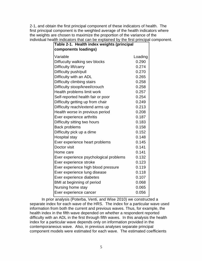
2-1, and obtain the first principal component of these indicators of health. The first principal component is the weighted average of the health indicators where the weights are chosen to maximize the proportion of the variance of the individual health indicators that can be explained by the first principal component.

Variable LoadingDiffuculty walking sev blocks 0.290Difficulty lift/carry 0.274Difficulty push/pull 0.270Difficulty with an ADL 0.265Difficulty climbing stairs 0.258Difficulty stoop/kneel/crouch 0.258Health problems limit work 0.257Self-reported health fair or poor 0.254Difficulty getting up from chair 0.249Difficulty reach/extend arms up 0.213Health worse in previous period 0.208Ever experience arthritis 0.187Difficulty sitting two hours 0.183Back problems 0.158Difficulty pick up a dime 0.152Hospital stay 0.148Ever experience heart problems 0.145Doctor visit 0.141Home care 0.141Ever experience psychological problems 0.132Ever experience stroke 0.123Ever experience high blood pressure 0.119Ever experience lung disease 0.118Ever experience diabetes 0.107BMI at beginning of period 0.068Nursing home stay 0.065Ever experience cancer 0.056

Table 2-1. Health index weights (principal components loadings)

In prior analysis (Poterba, Venti, and Wise 2010) we constructed a separate index for each wave of the HRS. The index for a particular wave used information from both the current and previous waves. Thus, for example, the health index in the fifth wave depended on whether a respondent reported difficulty with an ADL in the first through fifth waves. In this analysis the health index for a particular wave depends only on information provided in the contemporaneous wave. Also, in previous analyses separate principal component models were estimated for each wave. The estimated coefficients

6

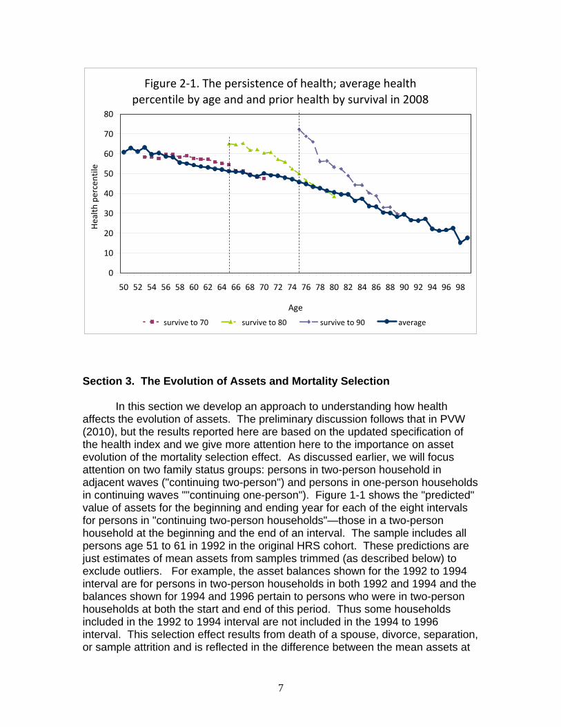
were very similar across waves, so in this analysis a single principal component equation is estimated from a sample that pools all of the waves. We use data from all of the HRS cohorts from 1992 through 2008 to estimate the single principal component model. The estimated coefficients are use to predict a "raw" health score for each respondent. For presentation purposes we convert these raw scores into a percentile scores for each respondent. We assign each person in a two-person household the minimum percentile score in the household because household health expenditures are likely to depend on the health of the partner in poorest health. This index, like the version used in our prior work, has several important properties for our purposes: 1) It is strongly related to the evolution of assets, as shown in Figure 3-3 through 3-6 below. 2) It is strongly related to mortality. 3) It is strongly predictive of future health events such as stroke and the onset of diabetes. 4) It is strongly related to economic outcomes prior to 1992, as well as to outcomes in 1992 and later. Some evidence in the ability of this index to predict subsequent mortality and to predict subsequent health events is provided in Poterba, Venti, and wise (2010). For the most part, the loadings on the HRS questions do not differ much between men and women or between married and single persons. The index can be used to show the very strong persistence of health. Figure 2-1 shows the average health percentile by age (the heavy blue line with round markers). This average health profile reflects two offsetting trends. Average health declines as people age, but this decline is offset by a selection effect: those in better health are more likely to survive from year to year. This selection effect is shown by the other curves in the figure. These show the average health in prior ages of those who survived until age 70, age 80 and age 90. It is clear that at each age those who survive longer are in better health. Those who survived until 80 had much better health at age 65 than the average of all of those who survived until 70, and that the health at age 75 of the persons who survive until 90 was much higher at age 75 than the health of all those who survived until 80.

7

Figure 2‐1. The persistence of health; average health percentile by age and and prior health by survival in 2008

0

10

20

30

40

50

60

70

80

50 52 54 56 58 60 62 64 66 68 70 72 74 76 78 80 82 84 86 88 90 92 94 96 98

Age

Health

percentile

survive to 70 survive to 80 survive to 90 average

Section 3. The Evolution of Assets and Mortality Selection

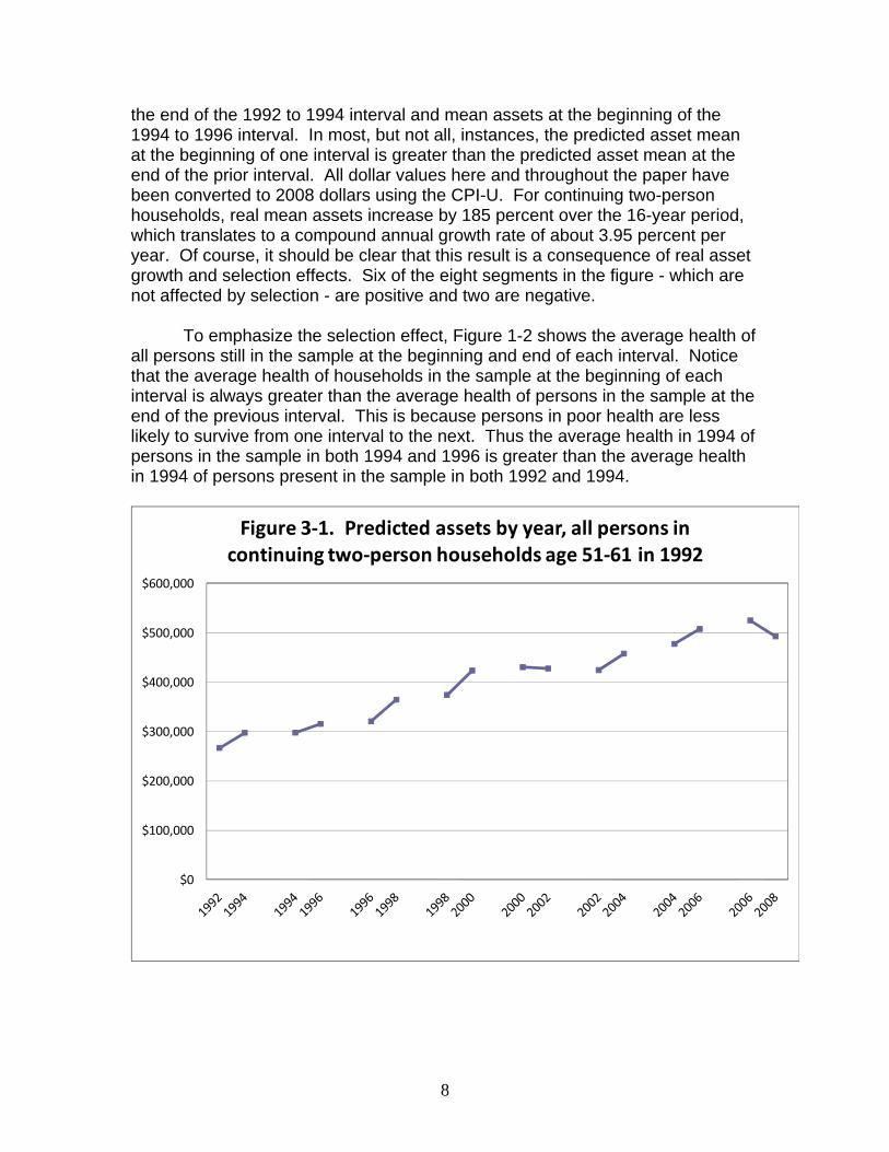
In this section we develop an approach to understanding how health affects the evolution of assets. The preliminary discussion follows that in PVW (2010), but the results reported here are based on the updated specification of the health index and we give more attention here to the importance on asset evolution of the mortality selection effect. As discussed earlier, we will focus attention on two family status groups: persons in two-person household in adjacent waves ("continuing two-person") and persons in one-person households in continuing waves ""continuing one-person"). Figure 1-1 shows the "predicted" value of assets for the beginning and ending year for each of the eight intervals for persons in "continuing two-person households"—those in a two-person household at the beginning and the end of an interval. The sample includes all persons age 51 to 61 in 1992 in the original HRS cohort. These predictions are just estimates of mean assets from samples trimmed (as described below) to exclude outliers. For example, the asset balances shown for the 1992 to 1994 interval are for persons in two-person households in both 1992 and 1994 and the balances shown for 1994 and 1996 pertain to persons who were in two-person households at both the start and end of this period. Thus some households included in the 1992 to 1994 interval are not included in the 1994 to 1996 interval. This selection effect results from death of a spouse, divorce, separation, or sample attrition and is reflected in the difference between the mean assets at

8

the end of the 1992 to 1994 interval and mean assets at the beginning of the 1994 to 1996 interval. In most, but not all, instances, the predicted asset mean at the beginning of one interval is greater than the predicted asset mean at the end of the prior interval. All dollar values here and throughout the paper have been converted to 2008 dollars using the CPI-U. For continuing two-person households, real mean assets increase by 185 percent over the 16-year period, which translates to a compound annual growth rate of about 3.95 percent per year. Of course, it should be clear that this result is a consequence of real asset growth and selection effects. Six of the eight segments in the figure - which are not affected by selection - are positive and two are negative.

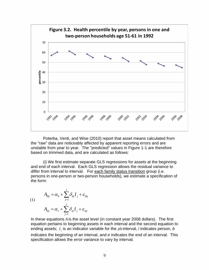
To emphasize the selection effect, Figure 1-2 shows the average health of

all persons still in the sample at the beginning and end of each interval. Notice that the average health of households in the sample at the beginning of each interval is always greater than the average health of persons in the sample at the end of the previous interval. This is because persons in poor health are less likely to survive from one interval to the next. Thus the average health in 1994 of persons in the sample in both 1994 and 1996 is greater than the average health in 1994 of persons present in the sample in both 1992 and 1994.

$0

$100,000

$200,000

$300,000

$400,000

$500,000

$600,000

Figure 3‐1. Predicted assets by year, all persons in continuing two‐person households age 51‐61 in 1992

9

0

10

20

30

40

50

60

70pe

rcen

tile

Figure 3.2. Health percentile by year, persons in one and two‐person households age 51‐61 in 1992

Poterba, Venti, and Wise (2010) report that asset means calculated from

the "raw" data are noticeably affected by apparent reporting errors and are unstable from year to year. The "predicted" values in Figure 1-1 are therefore based on trimmed data, and are calculated as follows:

(i) We first estimate separate GLS regressions for assets at the beginning

and end of each interval. Each GLS regression allows the residual variance to differ from interval to interval. For each family status transition group (i.e. persons in one-person or two-person households), we estimate a specification of the form:

1

1

J

ibj b bj j ibjj

J

iej e ej j iejj

A I

A I

α δ ε

α δ ε

=

=

= + +

= + +

∑

∑

In these equations A is the asset level (in constant year 2008 dollars). The first equation pertains to beginning assets in each interval and the second equation to ending assets; jI is an indicator variable for the jth interval, i indicates person, b indicates the beginning of an interval, and e indicates the end of an interval. This specification allows the error variance to vary by interval.

(1)

10

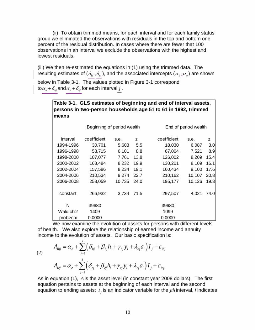
(ii) To obtain trimmed means, for each interval and for each family status group we eliminated the observations with residuals in the top and bottom one percent of the residual distribution. In cases where there are fewer that 100 observations in an interval we exclude the observations with the highest and lowest residuals. (iii) We then re-estimated the equations in (1) using the trimmed data. The resulting estimates of ( bjδ , ejδ ), and the associated intercepts ( bα , eα ) are shown

below in Table 3-1. The values plotted in Figure 3-1 correspond to b bjα δ+ and e ejα δ+ for each interval j .

interval coefficient s.e. z coefficient s.e. z1994-1996 30,701 5,603 5.5 18,030 6,087 3.01996-1998 53,715 6,101 8.8 67,004 7,521 8.91998-2000 107,077 7,761 13.8 126,002 8,209 15.42000-2002 163,484 8,232 19.9 130,201 8,109 16.12002-2004 157,586 8,234 19.1 160,434 9,100 17.62004-2006 210,534 9,274 22.7 210,162 10,107 20.82006-2008 258,059 10,735 24.0 195,177 10,126 19.3

constant 266,932 3,734 71.5 297,507 4,021 74.0

N 39680 39680Wald chi2 1409 1099prob>chi 0.0000 0.0000

Table 3-1. GLS estimates of beginning and end of interval assets, persons in two-person households age 51 to 61 in 1992, trimmed means

Beginning of period wealth End of period wealth

We now examine the evolution of assets for persons with different levels of health. We also explore the relationship of earned income and annuity income to the evolution of assets. Our basic specification is:

( )

( )1

1

J

ibj b bj bj i bj i bj i j ibjj

J

iej e ej ej i ej i ej i j iejj

A h y a I

A h y a I

α δ β γ λ ε

α δ β γ λ ε

=

=

= + + + + +

= + + + + +

∑

∑

As in equation (1), A is the asset level (in constant year 2008 dollars). The first equation pertains to assets at the beginning of each interval and the second equation to ending assets; jI is an indicator variable for the jth interval, i indicates

(2)

11

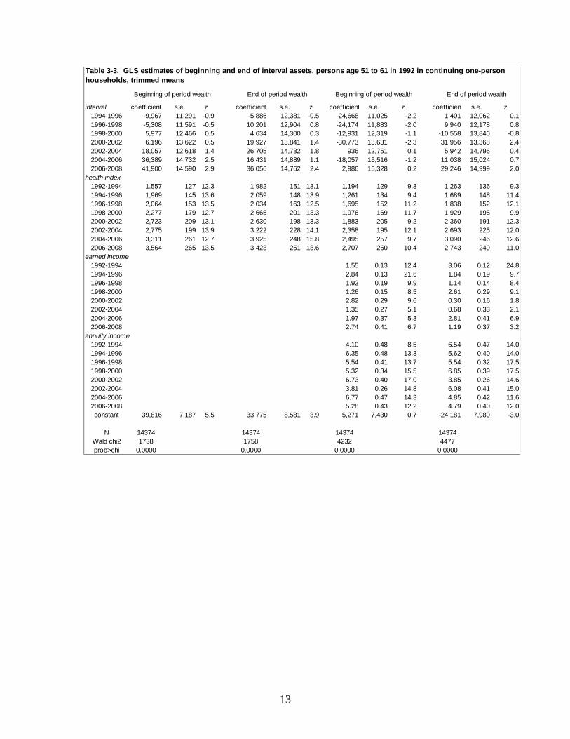
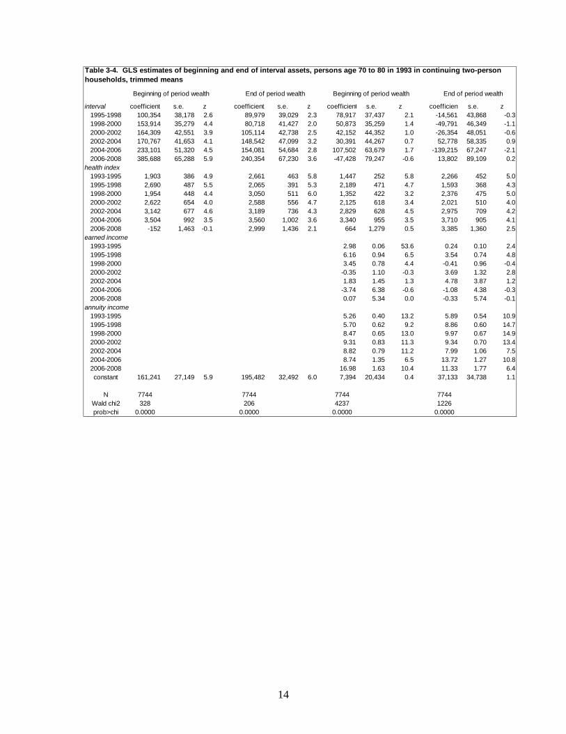
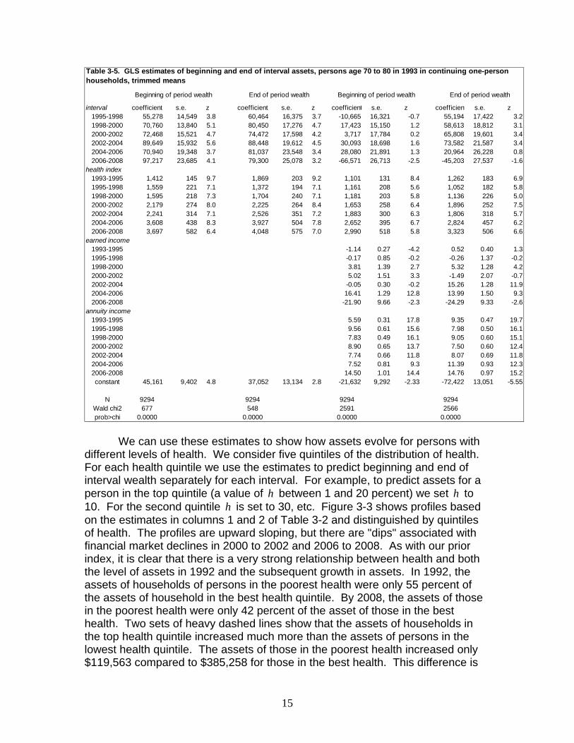
person, b indicates the beginning of an interval, and e indicates the end of an interval. In addition, h represents health, y represents earned income, and a represents annuity income. Health h is expressed as a percentile where the first percentile is the poorest health and the 100th percentile is the best health. Again the estimates are based on trimmed data, as described with respect to equation (1). Table 3-2 reports our estimation results, which differ from similar results in PVW (2010), because of the new health index used in this paper. The results in first two columns show estimates for health only, as well as indicator variables for each interval. The effect of health is very large and the estimates trend upward with year (age). For example, in the beginning year of an interval, an increase of one percentile in health is associated with an increase of assets of $1,849 in 1992 and $5,405 in 2006. For the ending year of an interval a one percentile increase in health translated to an asset increase of $2,288 in 1992 and by $5,170 in 2008. We have made similar estimates for HRS continuing one-person households, for AHEAD continuing two-person households, and for AHEAD continuing one-person households. The results are reported in Tables 3-3, 3-4, and 3-5 respectively.

12

interval coefficient s.e. z coefficient s.e. z coefficient s.e. z coefficient s.e. z1994-1996 -8,566 13,492 -0.6 -8,546 14,622 -0.6 27,500 12,770 2.2 -23,528 14,738 -1.61996-1998 8,824 14,066 0.6 16,522 17,283 1.0 19,107 13,977 1.4 -37,140 16,380 -2.31998-2000 14,366 17,631 0.8 38,343 18,632 2.1 -7,139 16,352 -0.4 -4,622 19,516 -0.22000-2002 54,069 18,487 2.9 39,960 18,169 2.2 52,515 19,473 2.7 10,014 19,330 0.52002-2004 54,718 17,989 3.0 57,337 19,840 2.9 45,401 19,012 2.4 16,725 18,886 0.92004-2006 78,962 19,599 4.0 76,726 21,282 3.6 16,279 21,207 0.8 21,916 22,532 1.02006-2008 108,185 22,693 4.8 80,837 21,448 3.8 92,636 24,028 3.9 27,232 22,855 1.2

health index1992-1994 1,849 140 13.2 2,288 150 15.3 901 123 7.3 1,496 141 10.61994-1996 2,359 153 15.4 2,562 167 15.3 1,462 144 10.2 1,999 162 12.41996-1998 2,576 170 15.2 3,108 225 13.8 1,990 163 12.2 2,289 195 11.81998-2000 3,525 245 14.4 3,885 258 15.1 2,693 210 12.8 3,275 251 13.02000-2002 3,939 268 14.7 4,042 255 15.8 3,459 263 13.2 3,401 251 13.62002-2004 4,043 271 14.9 4,540 302 15.0 3,259 264 12.4 3,517 277 12.72004-2006 4,849 316 15.3 5,406 345 15.7 3,808 303 12.6 4,424 334 13.32006-2008 5,405 391 13.8 5,170 359 14.4 4,507 381 11.8 4,196 349 12.0

earned income1992-1994 2.35 0.05 46.1 1.81 0.06 31.21994-1996 1.83 0.06 30.7 1.78 0.08 22.91996-1998 1.91 0.08 23.5 2.65 0.06 41.51998-2000 2.58 0.06 42.1 2.02 0.13 15.72000-2002 1.65 0.14 11.9 1.68 0.13 13.12002-2004 2.15 0.13 16.5 3.13 0.16 19.92004-2006 3.03 0.17 17.3 3.33 0.23 14.42006-2008 3.36 0.27 12.6 3.19 0.26 12.5

annuity income1992-1994 5.95 0.26 23.1 4.31 0.20 21.61994-1996 4.40 0.21 21.4 5.18 0.25 20.81996-1998 5.13 0.26 20.1 5.59 0.26 21.31998-2000 5.38 0.27 19.6 5.10 0.31 16.72000-2002 4.77 0.31 15.2 4.38 0.29 15.02002-2004 4.52 0.30 15.1 3.87 0.15 26.22004-2006 5.54 0.33 16.7 4.42 0.31 14.52006-2008 3.99 0.33 12.3 4.43 0.31 14.1constant 161,512 8,777 18.4 167,026 9,408 17.8 29,480 8,135 3.6 66,120 9,200 7.2

N 39680 39680 39680 39680Wald chi2 3186 2968 11337 9660prob>chi 0.0000 0.0000 0.0000 0.0000

Table 3-2. GLS estimates of beginning and end of interval assets, persons age 51 to 61 in 1992 in continuing two-person households, trimmed means

Beginning of period wealth End of period wealth Beginning of period wealth End of period wealth

13

interval coefficient s.e. z coefficient s.e. z coefficient s.e. z coefficient s.e. z1994-1996 -9,967 11,291 -0.9 -5,886 12,381 -0.5 -24,668 11,025 -2.2 1,401 12,062 0.11996-1998 -5,308 11,591 -0.5 10,201 12,904 0.8 -24,174 11,883 -2.0 9,940 12,178 0.81998-2000 5,977 12,466 0.5 4,634 14,300 0.3 -12,931 12,319 -1.1 -10,558 13,840 -0.82000-2002 6,196 13,622 0.5 19,927 13,841 1.4 -30,773 13,631 -2.3 31,956 13,368 2.42002-2004 18,057 12,618 1.4 26,705 14,732 1.8 936 12,751 0.1 5,942 14,796 0.42004-2006 36,389 14,732 2.5 16,431 14,889 1.1 -18,057 15,516 -1.2 11,038 15,024 0.72006-2008 41,900 14,590 2.9 36,056 14,762 2.4 2,986 15,328 0.2 29,246 14,999 2.0

health index1992-1994 1,557 127 12.3 1,982 151 13.1 1,194 129 9.3 1,263 136 9.31994-1996 1,969 145 13.6 2,059 148 13.9 1,261 134 9.4 1,689 148 11.41996-1998 2,064 153 13.5 2,034 163 12.5 1,695 152 11.2 1,838 152 12.11998-2000 2,277 179 12.7 2,665 201 13.3 1,976 169 11.7 1,929 195 9.92000-2002 2,723 209 13.1 2,630 198 13.3 1,883 205 9.2 2,360 191 12.32002-2004 2,775 199 13.9 3,222 228 14.1 2,358 195 12.1 2,693 225 12.02004-2006 3,311 261 12.7 3,925 248 15.8 2,495 257 9.7 3,090 246 12.62006-2008 3,564 265 13.5 3,423 251 13.6 2,707 260 10.4 2,743 249 11.0

earned income1992-1994 1.55 0.13 12.4 3.06 0.12 24.81994-1996 2.84 0.13 21.6 1.84 0.19 9.71996-1998 1.92 0.19 9.9 1.14 0.14 8.41998-2000 1.26 0.15 8.5 2.61 0.29 9.12000-2002 2.82 0.29 9.6 0.30 0.16 1.82002-2004 1.35 0.27 5.1 0.68 0.33 2.12004-2006 1.97 0.37 5.3 2.81 0.41 6.92006-2008 2.74 0.41 6.7 1.19 0.37 3.2

annuity income1992-1994 4.10 0.48 8.5 6.54 0.47 14.01994-1996 6.35 0.48 13.3 5.62 0.40 14.01996-1998 5.54 0.41 13.7 5.54 0.32 17.51998-2000 5.32 0.34 15.5 6.85 0.39 17.52000-2002 6.73 0.40 17.0 3.85 0.26 14.62002-2004 3.81 0.26 14.8 6.08 0.41 15.02004-2006 6.77 0.47 14.3 4.85 0.42 11.62006-2008 5.28 0.43 12.2 4.79 0.40 12.0constant 39,816 7,187 5.5 33,775 8,581 3.9 5,271 7,430 0.7 -24,181 7,980 -3.0


Table 3-3. GLS estimates of beginning and end of interval assets, persons age 51 to 61 in 1992 in continuing one-person households, trimmed means


14

interval coefficient s.e. z coefficient s.e. z coefficient s.e. z coefficient s.e. z1995-1998 100,354 38,178 2.6 89,979 39,029 2.3 78,917 37,437 2.1 -14,561 43,868 -0.31998-2000 153,914 35,279 4.4 80,718 41,427 2.0 50,873 35,259 1.4 -49,791 46,349 -1.12000-2002 164,309 42,551 3.9 105,114 42,738 2.5 42,152 44,352 1.0 -26,354 48,051 -0.62002-2004 170,767 41,653 4.1 148,542 47,099 3.2 30,391 44,267 0.7 52,778 58,335 0.92004-2006 233,101 51,320 4.5 154,081 54,684 2.8 107,502 63,679 1.7 -139,215 67,247 -2.12006-2008 385,688 65,288 5.9 240,354 67,230 3.6 -47,428 79,247 -0.6 13,802 89,109 0.2

health index1993-1995 1,903 386 4.9 2,661 463 5.8 1,447 252 5.8 2,266 452 5.01995-1998 2,690 487 5.5 2,065 391 5.3 2,189 471 4.7 1,593 368 4.31998-2000 1,954 448 4.4 3,050 511 6.0 1,352 422 3.2 2,376 475 5.02000-2002 2,622 654 4.0 2,588 556 4.7 2,125 618 3.4 2,021 510 4.02002-2004 3,142 677 4.6 3,189 736 4.3 2,829 628 4.5 2,975 709 4.22004-2006 3,504 992 3.5 3,560 1,002 3.6 3,340 955 3.5 3,710 905 4.12006-2008 -152 1,463 -0.1 2,999 1,436 2.1 664 1,279 0.5 3,385 1,360 2.5

earned income1993-1995 2.98 0.06 53.6 0.24 0.10 2.41995-1998 6.16 0.94 6.5 3.54 0.74 4.81998-2000 3.45 0.78 4.4 -0.41 0.96 -0.42000-2002 -0.35 1.10 -0.3 3.69 1.32 2.82002-2004 1.83 1.45 1.3 4.78 3.87 1.22004-2006 -3.74 6.38 -0.6 -1.08 4.38 -0.32006-2008 0.07 5.34 0.0 -0.33 5.74 -0.1

annuity income1993-1995 5.26 0.40 13.2 5.89 0.54 10.91995-1998 5.70 0.62 9.2 8.86 0.60 14.71998-2000 8.47 0.65 13.0 9.97 0.67 14.92000-2002 9.31 0.83 11.3 9.34 0.70 13.42002-2004 8.82 0.79 11.2 7.99 1.06 7.52004-2006 8.74 1.35 6.5 13.72 1.27 10.82006-2008 16.98 1.63 10.4 11.33 1.77 6.4constant 161,241 27,149 5.9 195,482 32,492 6.0 7,394 20,434 0.4 37,133 34,738 1.1


Table 3-4. GLS estimates of beginning and end of interval assets, persons age 70 to 80 in 1993 in continuing two-person households, trimmed means


15

interval coefficient s.e. z coefficient s.e. z coefficient s.e. z coefficient s.e. z1995-1998 55,278 14,549 3.8 60,464 16,375 3.7 -10,665 16,321 -0.7 55,194 17,422 3.21998-2000 70,760 13,840 5.1 80,450 17,276 4.7 17,423 15,150 1.2 58,613 18,812 3.12000-2002 72,468 15,521 4.7 74,472 17,598 4.2 3,717 17,784 0.2 65,808 19,601 3.42002-2004 89,649 15,932 5.6 88,448 19,612 4.5 30,093 18,698 1.6 73,582 21,587 3.42004-2006 70,940 19,348 3.7 81,037 23,548 3.4 28,080 21,891 1.3 20,964 26,228 0.82006-2008 97,217 23,685 4.1 79,300 25,078 3.2 -66,571 26,713 -2.5 -45,203 27,537 -1.6

health index1993-1995 1,412 145 9.7 1,869 203 9.2 1,101 131 8.4 1,262 183 6.91995-1998 1,559 221 7.1 1,372 194 7.1 1,161 208 5.6 1,052 182 5.81998-2000 1,595 218 7.3 1,704 240 7.1 1,181 203 5.8 1,136 226 5.02000-2002 2,179 274 8.0 2,225 264 8.4 1,653 258 6.4 1,896 252 7.52002-2004 2,241 314 7.1 2,526 351 7.2 1,883 300 6.3 1,806 318 5.72004-2006 3,608 438 8.3 3,927 504 7.8 2,652 395 6.7 2,824 457 6.22006-2008 3,697 582 6.4 4,048 575 7.0 2,990 518 5.8 3,323 506 6.6

earned income1993-1995 -1.14 0.27 -4.2 0.52 0.40 1.31995-1998 -0.17 0.85 -0.2 -0.26 1.37 -0.21998-2000 3.81 1.39 2.7 5.32 1.28 4.22000-2002 5.02 1.51 3.3 -1.49 2.07 -0.72002-2004 -0.05 0.30 -0.2 15.26 1.28 11.92004-2006 16.41 1.29 12.8 13.99 1.50 9.32006-2008 -21.90 9.66 -2.3 -24.29 9.33 -2.6

annuity income1993-1995 5.59 0.31 17.8 9.35 0.47 19.71995-1998 9.56 0.61 15.6 7.98 0.50 16.11998-2000 7.83 0.49 16.1 9.05 0.60 15.12000-2002 8.90 0.65 13.7 7.50 0.60 12.42002-2004 7.74 0.66 11.8 8.07 0.69 11.82004-2006 7.52 0.81 9.3 11.39 0.93 12.32006-2008 14.50 1.01 14.4 14.76 0.97 15.2constant 45,161 9,402 4.8 37,052 13,134 2.8 -21,632 9,292 -2.33 -72,422 13,051 -5.55


Table 3-5. GLS estimates of beginning and end of interval assets, persons age 70 to 80 in 1993 in continuing one-person households, trimmed means


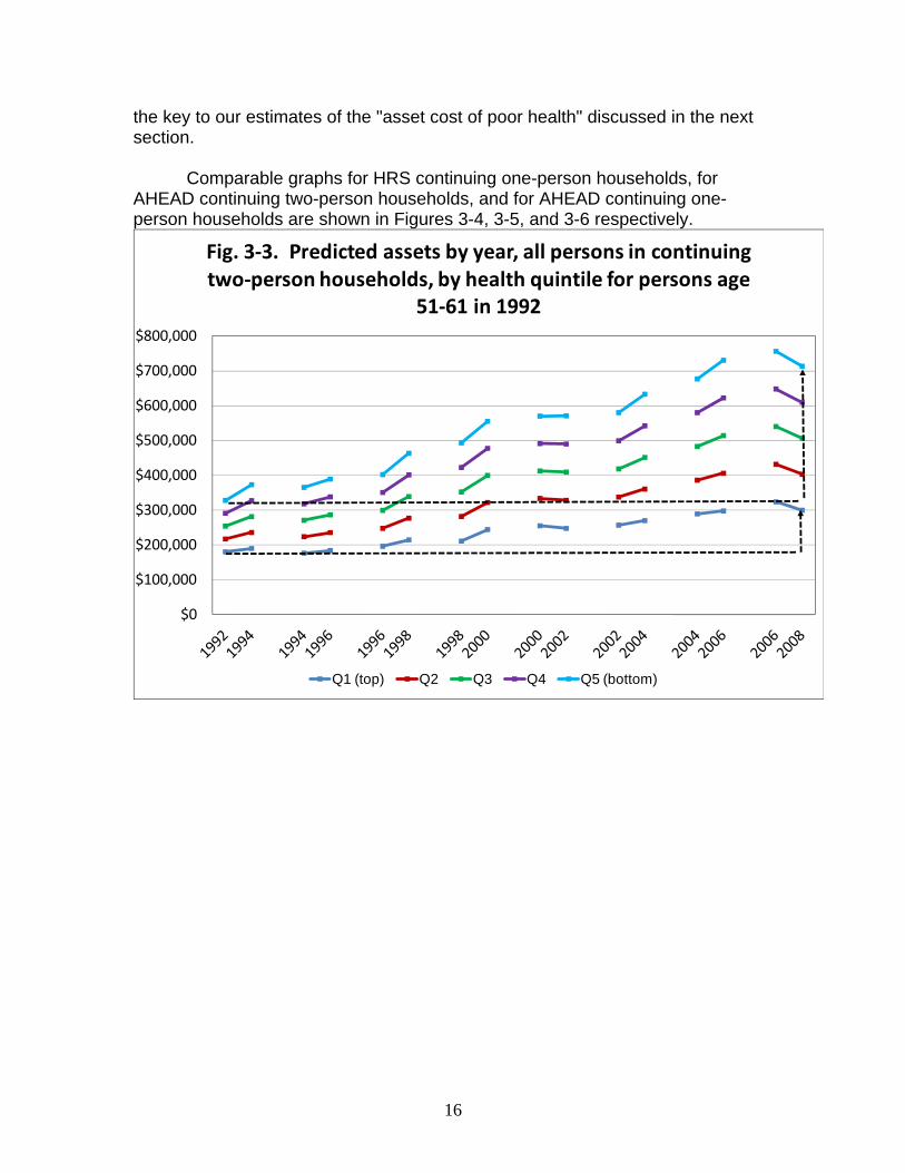
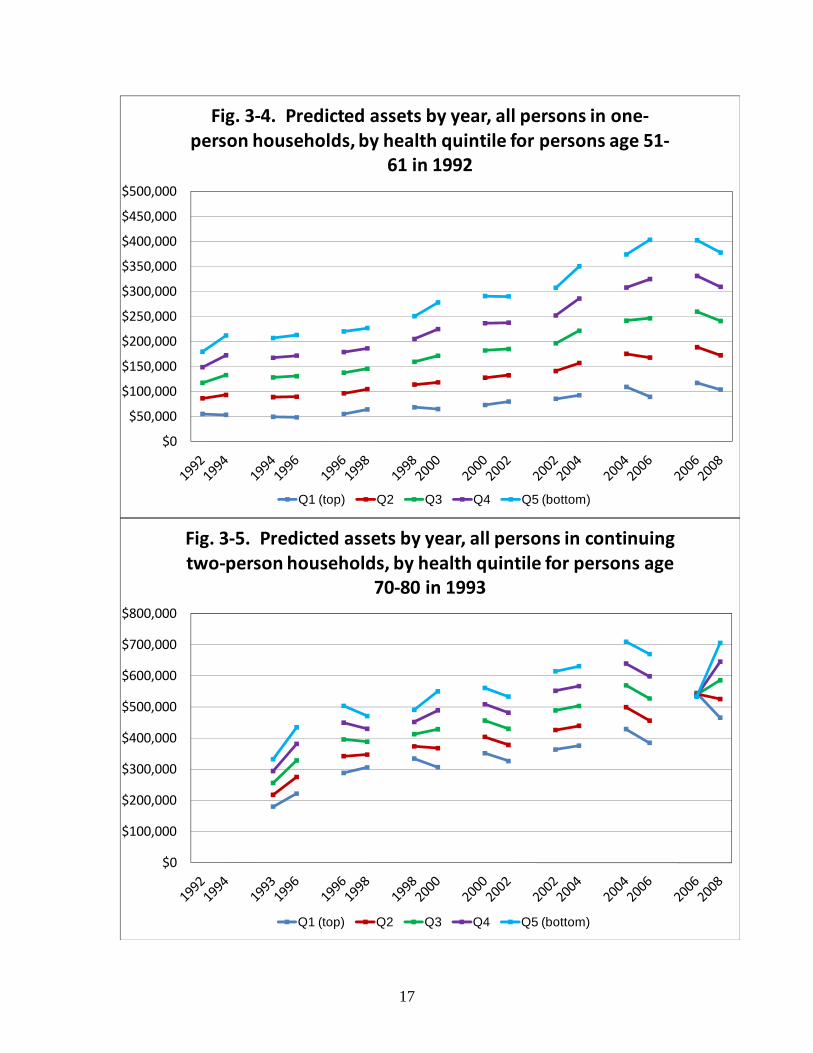
We can use these estimates to show how assets evolve for persons with different levels of health. We consider five quintiles of the distribution of health. For each health quintile we use the estimates to predict beginning and end of interval wealth separately for each interval. For example, to predict assets for a person in the top quintile (a value of h between 1 and 20 percent) we set h to 10. For the second quintile h is set to 30, etc. Figure 3-3 shows profiles based on the estimates in columns 1 and 2 of Table 3-2 and distinguished by quintiles of health. The profiles are upward sloping, but there are "dips" associated with financial market declines in 2000 to 2002 and 2006 to 2008. As with our prior index, it is clear that there is a very strong relationship between health and both the level of assets in 1992 and the subsequent growth in assets. In 1992, the assets of households of persons in the poorest health were only 55 percent of the assets of household in the best health quintile. By 2008, the assets of those in the poorest health were only 42 percent of the asset of those in the best health. Two sets of heavy dashed lines show that the assets of households in the top health quintile increased much more than the assets of persons in the lowest health quintile. The assets of those in the poorest health increased only $119,563 compared to $385,258 for those in the best health. This difference is

16

the key to our estimates of the "asset cost of poor health" discussed in the next section.

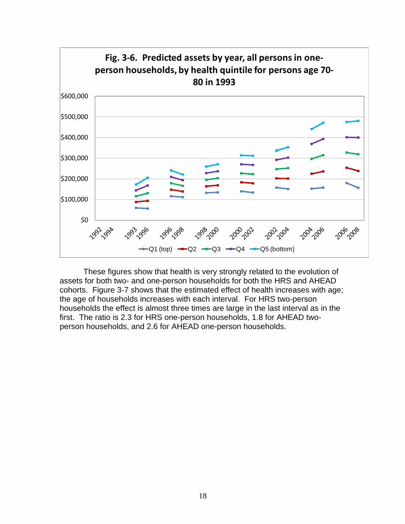
Comparable graphs for HRS continuing one-person households, for

AHEAD continuing two-person households, and for AHEAD continuing one-person households are shown in Figures 3-4, 3-5, and 3-6 respectively.

$0

$100,000

$200,000

$300,000

$400,000

$500,000

$600,000

$700,000

$800,000

Fig. 3‐3. Predicted assets by year, all persons in continuing two‐person households, by health quintile for persons age

51‐61 in 1992

Q1 (top) Q2 Q3 Q4 Q5 (bottom)

17

$0

$50,000

$100,000

$150,000

$200,000

$250,000

$300,000

$350,000

$400,000

$450,000

$500,000

Fig. 3‐4. Predicted assets by year, all persons in one‐person households, by health quintile for persons age 51‐

61 in 1992


$0

$100,000

$200,000

$300,000

$400,000

$500,000

$600,000

$700,000

$800,000

Fig. 3‐5. Predicted assets by year, all persons in continuing two‐person households, by health quintile for persons age

70‐80 in 1993


18

$0

$100,000

$200,000

$300,000

$400,000

$500,000

$600,000

Fig. 3‐6. Predicted assets by year, all persons in one‐person households, by health quintile for persons age 70‐

80 in 1993


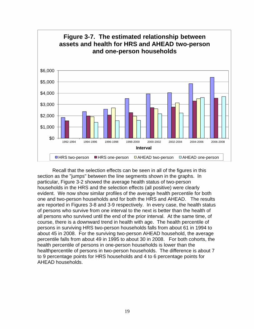
These figures show that health is very strongly related to the evolution of

assets for both two- and one-person households for both the HRS and AHEAD cohorts. Figure 3-7 shows that the estimated effect of health increases with age; the age of households increases with each interval. For HRS two-person households the effect is almost three times are large in the last interval as in the first. The ratio is 2.3 for HRS one-person households, 1.8 for AHEAD two- person households, and 2.6 for AHEAD one-person households.

19

$0

$1,000

$2,000

$3,000

$4,000

$5,000

$6,000

1992-1994 1994-1996 1996-1998 1998-2000 2000-2002 2002-2004 2004-2006 2006-2008

Interval

Figure 3-7. The estimated relationship between assets and health for HRS and AHEAD two-person

and one-person households

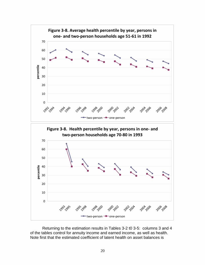
HRS two-person HRS one-person AHEAD two-person AHEAD one-person Recall that the selection effects can be seen in all of the figures in this

section as the "jumps" between the line segments shown in the graphs. In particular, Figure 3-2 showed the average health status of two-person households in the HRS and the selection effects (all positive) were clearly evident. We now show similar profiles of the average health percentile for both one and two-person households and for both the HRS and AHEAD. The results are reported in Figures 3-8 and 3-9 respectively. In every case, the health status of persons who survive from one interval to the next is better than the health of all persons who survived until the end of the prior interval. At the same time, of course, there is a downward trend in health with age. The health percentile of persons in surviving HRS two-person households falls from about 61 in 1994 to about 45 in 2008. For the surviving two-person AHEAD household, the average percentile falls from about 49 in 1995 to about 30 in 2008. For both cohorts, the health percentile of persons in one-person households is lower than the healthpercentile of persons in two-person households. The difference is about 7 to 9 percentage points for HRS households and 4 to 6 percentage points for AHEAD households.

20

Figure 3‐8. Average health percentile by year, persons in one‐ and two‐person households age 51‐61 in 1992

0

10

20

30

40

50

60

70

19921994

19941996

19961998

19982000

20002002

20022004

20042006

20062008

percen

tile

two‐person one‐person

Figure 3‐8. Health percentile by year, persons in one‐ and two‐person households age 70‐80 in 1993

0

10

20

30

40

50

60

70

19931995

19951998

19982000

20002002

20022004

20042006

20062008

percen

tile

two‐person one‐person

Returning to the estimation results in Tables 3-2 t0 3-5: columns 3 and 4

of the tables control for annuity income and earned income, as well as health. Note first that the estimated coefficient of latent health on asset balances is

21

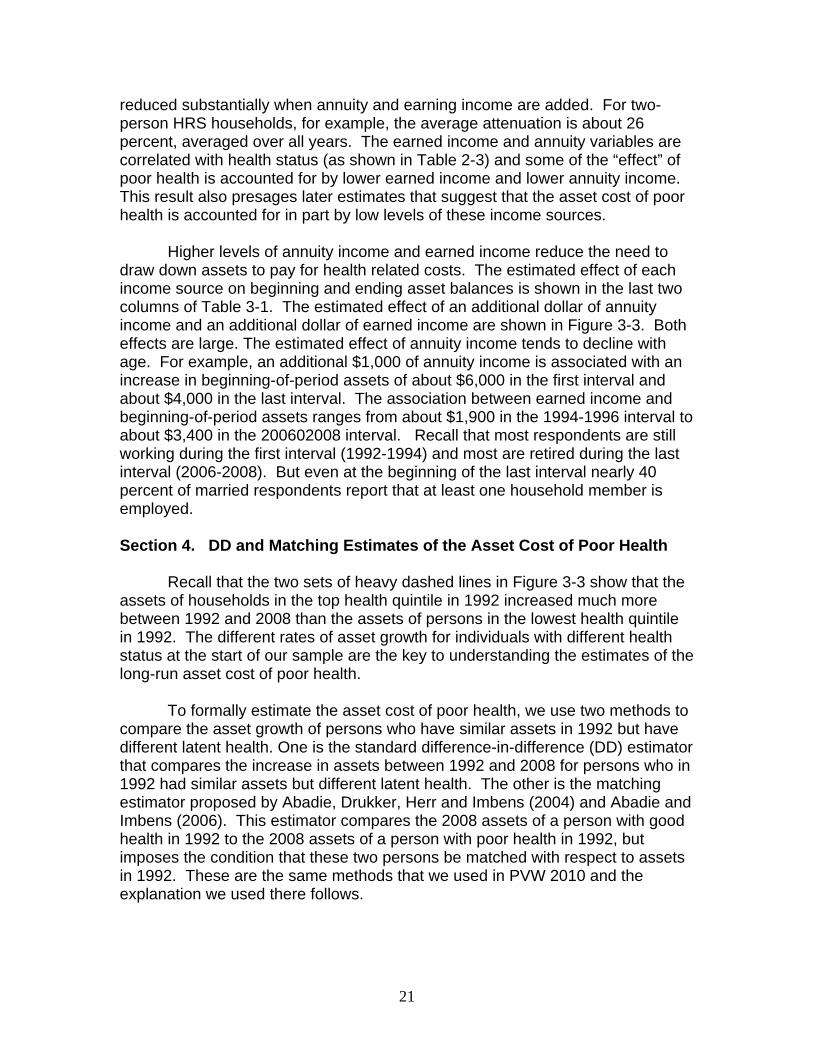
reduced substantially when annuity and earning income are added. For two-person HRS households, for example, the average attenuation is about 26 percent, averaged over all years. The earned income and annuity variables are correlated with health status (as shown in Table 2-3) and some of the “effect” of poor health is accounted for by lower earned income and lower annuity income. This result also presages later estimates that suggest that the asset cost of poor health is accounted for in part by low levels of these income sources.

Higher levels of annuity income and earned income reduce the need to

draw down assets to pay for health related costs. The estimated effect of each income source on beginning and ending asset balances is shown in the last two columns of Table 3-1. The estimated effect of an additional dollar of annuity income and an additional dollar of earned income are shown in Figure 3-3. Both effects are large. The estimated effect of annuity income tends to decline with age. For example, an additional $1,000 of annuity income is associated with an increase in beginning-of-period assets of about $6,000 in the first interval and about $4,000 in the last interval. The association between earned income and beginning-of-period assets ranges from about $1,900 in the 1994-1996 interval to about $3,400 in the 200602008 interval. Recall that most respondents are still working during the first interval (1992-1994) and most are retired during the last interval (2006-2008). But even at the beginning of the last interval nearly 40 percent of married respondents report that at least one household member is employed. Section 4. DD and Matching Estimates of the Asset Cost of Poor Health

Recall that the two sets of heavy dashed lines in Figure 3-3 show that the assets of households in the top health quintile in 1992 increased much more between 1992 and 2008 than the assets of persons in the lowest health quintile in 1992. The different rates of asset growth for individuals with different health status at the start of our sample are the key to understanding the estimates of the long-run asset cost of poor health.

To formally estimate the asset cost of poor health, we use two methods to

compare the asset growth of persons who have similar assets in 1992 but have different latent health. One is the standard difference-in-difference (DD) estimator that compares the increase in assets between 1992 and 2008 for persons who in 1992 had similar assets but different latent health. The other is the matching estimator proposed by Abadie, Drukker, Herr and Imbens (2004) and Abadie and Imbens (2006). This estimator compares the 2008 assets of a person with good health in 1992 to the 2008 assets of a person with poor health in 1992, but imposes the condition that these two persons be matched with respect to assets in 1992. These are the same methods that we used in PVW 2010 and the explanation we used there follows.

22

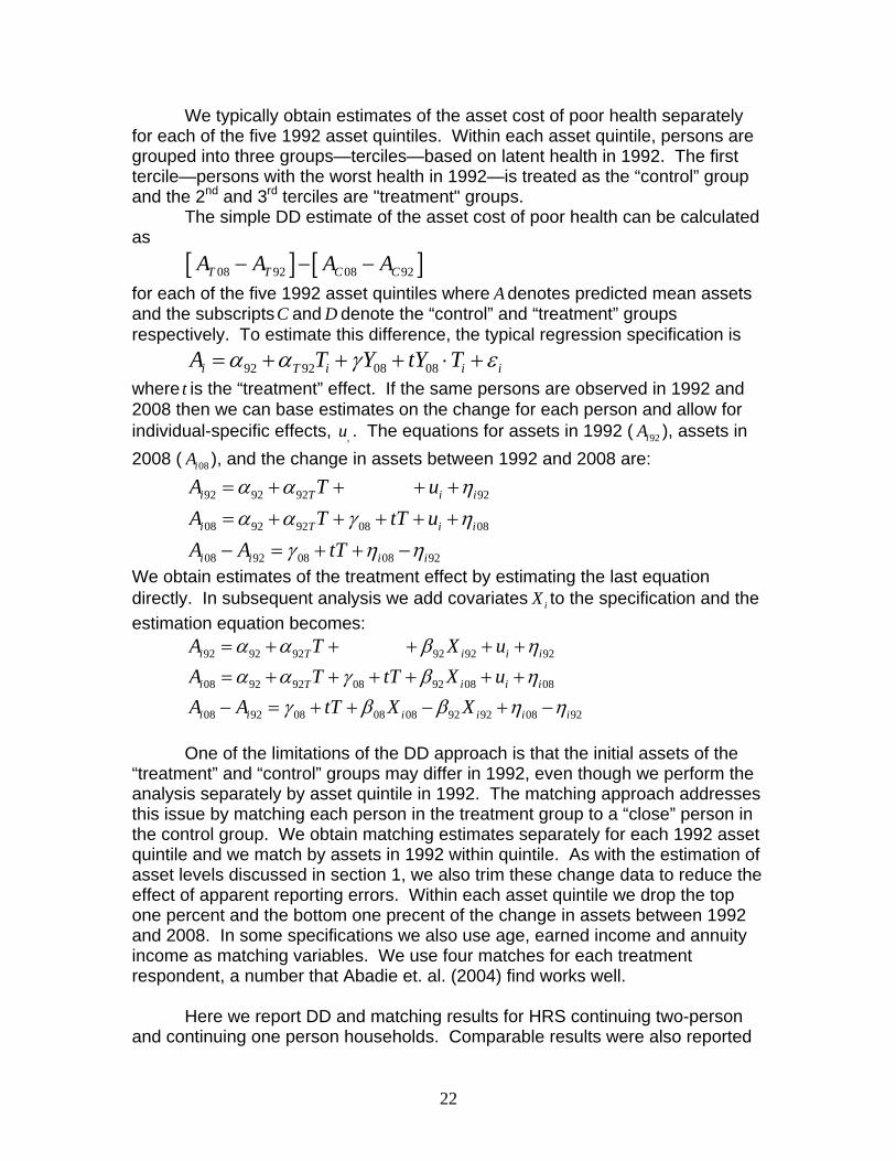
We typically obtain estimates of the asset cost of poor health separately for each of the five 1992 asset quintiles. Within each asset quintile, persons are grouped into three groups—terciles—based on latent health in 1992. The first tercile—persons with the worst health in 1992—is treated as the “control” group and the 2nd and 3rd terciles are "treatment" groups.

The simple DD estimate of the asset cost of poor health can be calculated as

[ ] [ ]08 92 08 92T T C CA A A A− − − for each of the five 1992 asset quintiles where A denotes predicted mean assets and the subscriptsC and D denote the “control” and “treatment” groups respectively. To estimate this difference, the typical regression specification is

92 92 08 08i T i i iA T Y tY Tα α γ ε= + + + ⋅ + where t is the “treatment” effect. If the same persons are observed in 1992 and 2008 then we can base estimates on the change for each person and allow for individual-specific effects, ,u . The equations for assets in 1992 ( 92iA ), assets in 2008 ( 08iA ), and the change in assets between 1992 and 2008 are:

92 92 92 92

08 92 92 08 08

08 92 08 08 92

i T i i

i T i i

i i i i

A T uA T tT uA A tT

α α ηα α γ η

γ η η

= + + + +

= + + + + +

− = + + −

We obtain estimates of the treatment effect by estimating the last equation directly. In subsequent analysis we add covariates iX to the specification and the estimation equation becomes:

92 92 92 92 92 92

08 92 92 08 92 08 08

08 92 08 08 08 92 92 08 92

i T i i i

i T i i i

i i i i i i

A T X uA T tT X uA A tT X X

α α β ηα α γ β η

γ β β η η

= + + + + +

= + + + + + +− = + + − + −

One of the limitations of the DD approach is that the initial assets of the

“treatment” and “control” groups may differ in 1992, even though we perform the analysis separately by asset quintile in 1992. The matching approach addresses this issue by matching each person in the treatment group to a “close” person in the control group. We obtain matching estimates separately for each 1992 asset quintile and we match by assets in 1992 within quintile. As with the estimation of asset levels discussed in section 1, we also trim these change data to reduce the effect of apparent reporting errors. Within each asset quintile we drop the top one percent and the bottom one precent of the change in assets between 1992 and 2008. In some specifications we also use age, earned income and annuity income as matching variables. We use four matches for each treatment respondent, a number that Abadie et. al. (2004) find works well. Here we report DD and matching results for HRS continuing two-person and continuing one person households. Comparable results were also reported

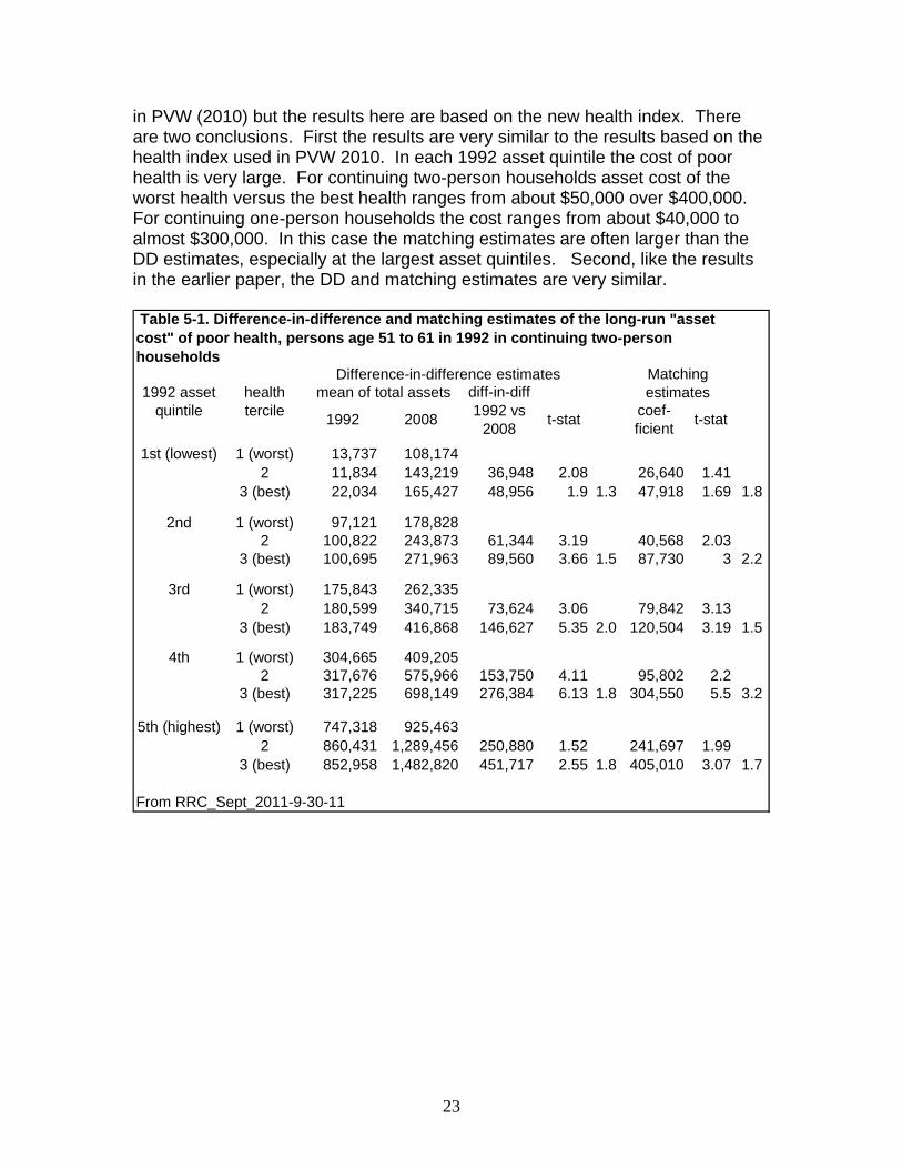
23

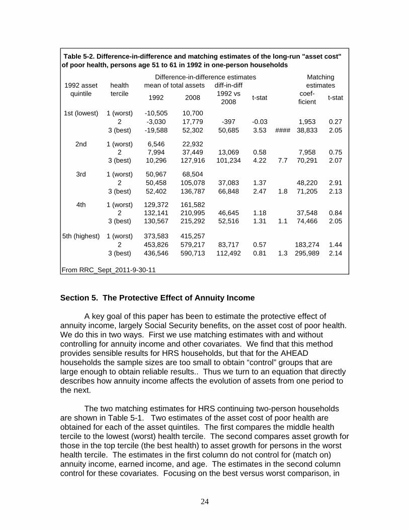
in PVW (2010) but the results here are based on the new health index. There are two conclusions. First the results are very similar to the results based on the health index used in PVW 2010. In each 1992 asset quintile the cost of poor health is very large. For continuing two-person households asset cost of the worst health versus the best health ranges from about $50,000 over $400,000. For continuing one-person households the cost ranges from about $40,000 to almost $300,000. In this case the matching estimates are often larger than the DD estimates, especially at the largest asset quintiles. Second, like the results in the earlier paper, the DD and matching estimates are very similar.

1st (lowest) 1 (worst) 13,737 108,1742 11,834 143,219 36,948 2.08 26,640 1.41

3 (best) 22,034 165,427 48,956 1.9 1.3 47,918 1.69 1.8

2nd 1 (worst) 97,121 178,8282 100,822 243,873 61,344 3.19 40,568 2.03

3 (best) 100,695 271,963 89,560 3.66 1.5 87,730 3 2.2

3rd 1 (worst) 175,843 262,3352 180,599 340,715 73,624 3.06 79,842 3.13

3 (best) 183,749 416,868 146,627 5.35 2.0 120,504 3.19 1.5

4th 1 (worst) 304,665 409,2052 317,676 575,966 153,750 4.11 95,802 2.2

3 (best) 317,225 698,149 276,384 6.13 1.8 304,550 5.5 3.2

5th (highest) 1 (worst) 747,318 925,4632 860,431 1,289,456 250,880 1.52 241,697 1.99

3 (best) 852,958 1,482,820 451,717 2.55 1.8 405,010 3.07 1.7

From RRC_Sept_2011-9-30-11

Table 5-1. Difference-in-difference and matching estimates of the long-run "asset cost" of poor health, persons age 51 to 61 in 1992 in continuing two-person households

1992 asset quintile

health tercile

Difference-in-difference estimates Matching estimatesmean of total assets

1992 2008 t-stat coef-ficient t-stat

diff-in-diff 1992 vs

2008

24

1st (lowest) 1 (worst) -10,505 10,7002 -3,030 17,779 -397 -0.03 1,953 0.27

3 (best) -19,588 52,302 50,685 3.53 #### 38,833 2.05

2nd 1 (worst) 6,546 22,9322 7,994 37,449 13,069 0.58 7,958 0.75

3 (best) 10,296 127,916 101,234 4.22 7.7 70,291 2.07

3rd 1 (worst) 50,967 68,5042 50,458 105,078 37,083 1.37 48,220 2.91

3 (best) 52,402 136,787 66,848 2.47 1.8 71,205 2.13

4th 1 (worst) 129,372 161,5822 132,141 210,995 46,645 1.18 37,548 0.84

3 (best) 130,567 215,292 52,516 1.31 1.1 74,466 2.05

5th (highest) 1 (worst) 373,583 415,2572 453,826 579,217 83,717 0.57 183,274 1.44

3 (best) 436,546 590,713 112,492 0.81 1.3 295,989 2.14

From RRC_Sept_2011-9-30-11

t-stat

mean of total assets diff-in-diff 1992 vs

20081992

Table 5-2. Difference-in-difference and matching estimates of the long-run "asset cost" of poor health, persons age 51 to 61 in 1992 in one-person households

1992 asset quintile

health tercile

Difference-in-difference estimates Matching estimates

2008 t-stat coef-ficient

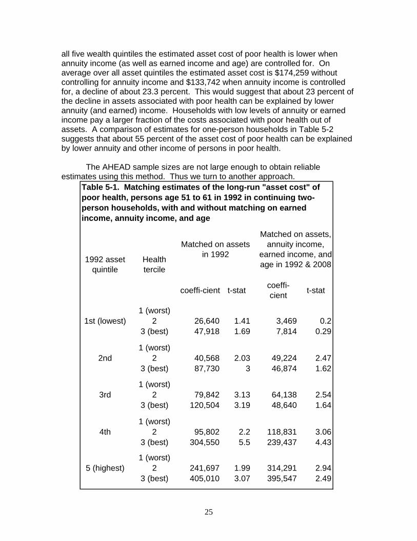
Section 5. The Protective Effect of Annuity Income A key goal of this paper has been to estimate the protective effect of annuity income, largely Social Security benefits, on the asset cost of poor health. We do this in two ways. First we use matching estimates with and without controlling for annuity income and other covariates. We find that this method provides sensible results for HRS households, but that for the AHEAD households the sample sizes are too small to obtain “control” groups that are large enough to obtain reliable results.. Thus we turn to an equation that directly describes how annuity income affects the evolution of assets from one period to the next. The two matching estimates for HRS continuing two-person households are shown in Table 5-1. Two estimates of the asset cost of poor health are obtained for each of the asset quintiles. The first compares the middle health tercile to the lowest (worst) health tercile. The second compares asset growth for those in the top tercile (the best health) to asset growth for persons in the worst health tercile. The estimates in the first column do not control for (match on) annuity income, earned income, and age. The estimates in the second column control for these covariates. Focusing on the best versus worst comparison, in

25

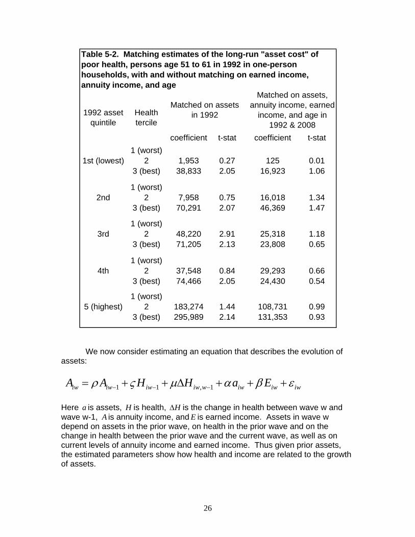
all five wealth quintiles the estimated asset cost of poor health is lower when annuity income (as well as earned income and age) are controlled for. On average over all asset quintiles the estimated asset cost is $174,259 without controlling for annuity income and $133,742 when annuity income is controlled for, a decline of about 23.3 percent. This would suggest that about 23 percent of the decline in assets associated with poor health can be explained by lower annuity (and earned) income. Households with low levels of annuity or earned income pay a larger fraction of the costs associated with poor health out of assets. A comparison of estimates for one-person households in Table 5-2 suggests that about 55 percent of the asset cost of poor health can be explained by lower annuity and other income of persons in poor health. The AHEAD sample sizes are not large enough to obtain reliable estimates using this method. Thus we turn to another approach.

coeffi-cient t-stat coeffi-cient t-stat

1 (worst)1st (lowest) 2 26,640 1.41 3,469 0.2

3 (best) 47,918 1.69 7,814 0.29

1 (worst)2nd 2 40,568 2.03 49,224 2.47

3 (best) 87,730 3 46,874 1.62

1 (worst)3rd 2 79,842 3.13 64,138 2.54

3 (best) 120,504 3.19 48,640 1.64

1 (worst)4th 2 95,802 2.2 118,831 3.06

3 (best) 304,550 5.5 239,437 4.43

1 (worst)5 (highest) 2 241,697 1.99 314,291 2.94

3 (best) 405,010 3.07 395,547 2.49

Table 5-1. Matching estimates of the long-run "asset cost" of poor health, persons age 51 to 61 in 1992 in continuing two-person households, with and without matching on earned income, annuity income, and age

1992 asset quintile

Health tercile

Matched on assets in 1992

Matched on assets, annuity income,

earned income, and age in 1992 & 2008

26

coefficient t-stat coefficient t-stat1 (worst)

1st (lowest) 2 1,953 0.27 125 0.013 (best) 38,833 2.05 16,923 1.06

1 (worst)2nd 2 7,958 0.75 16,018 1.34

3 (best) 70,291 2.07 46,369 1.47

1 (worst)3rd 2 48,220 2.91 25,318 1.18

3 (best) 71,205 2.13 23,808 0.65

1 (worst)4th 2 37,548 0.84 29,293 0.66

3 (best) 74,466 2.05 24,430 0.54

1 (worst)5 (highest) 2 183,274 1.44 108,731 0.99

3 (best) 295,989 2.14 131,353 0.93

Table 5-2. Matching estimates of the long-run "asset cost" of poor health, persons age 51 to 61 in 1992 in one-person households, with and without matching on earned income, annuity income, and age

1992 asset quintile

Health tercile

Matched on assets in 1992

Matched on assets, annuity income, earned

income, and age in 1992 & 2008

We now consider estimating an equation that describes the evolution of assets:

1 1 , 1iw iw iw iw w iw iw iwA A H H a Eρ ς μ α β ε− − −= + + Δ + + + Here a is assets, H is health, HΔ is the change in health between wave w and wave w-1, A is annuity income, and E is earned income. Assets in wave w depend on assets in the prior wave, on health in the prior wave and on the change in health between the prior wave and the current wave, as well as on current levels of annuity income and earned income. Thus given prior assets, the estimated parameters show how health and income are related to the growth of assets.

27

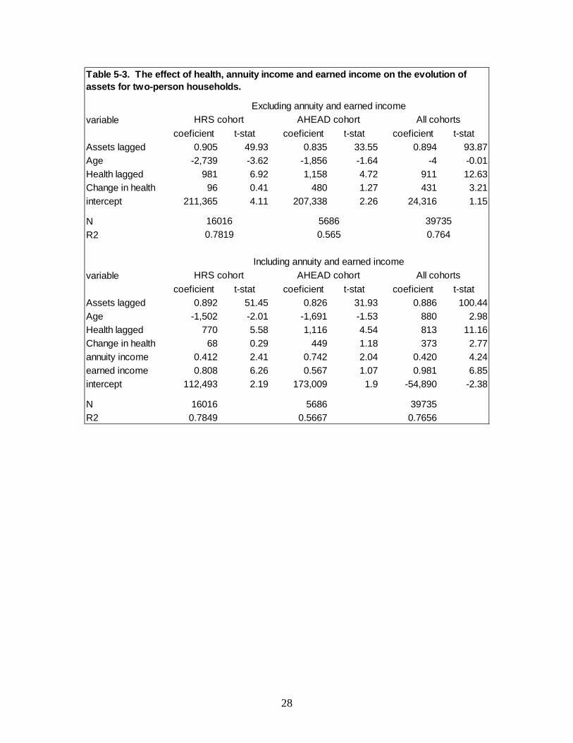
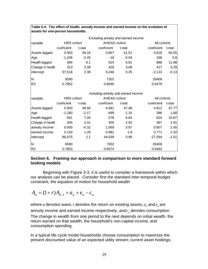
We use this equation to obtain three sets of estimates: a set for one and two-person households in the HRS, another set for one and two-person households in the AHEAD, and a third set that includes one and two-person households in all of the HRS cohorts (HRS, AHEAD, WB, CODA, and EBB). For all three sets of estimates we restrict the analysis to persons age 65 or older. As before, we trim the data to limit the influence of outliers. The top and bottom one-percent of asset values in each wave are deleted prior to estimation. The results are shown in Table 5-3 for two-person households and in Table 5-4 for one-person households. In each table the estimates in the top panel do not control for annuity and earned income. The estimates in the bottom panel control for these variables. First, when only lagged health and the change in health are included a 10 percentile increase in the health index is associated with a wave-to-wave increase of $10,000 in assets for two-person households and between $5,840 and $8,880 for one-person households. When annuity income and earned income are added the estimated coefficient on health falls for all three cohorts, but the decline is rather small: -21.5% for the HRS cohort, -3.6% for the AHEAD cohort and -10.8% for all the broader sample that includes all of the HRS cohorts. For one-person households the percent declines in the effect of health are -3.9%, -7.4%, and -7.2% for the three samples. The estimated effect of lagged health is statistically significant in each case for two-person households and for all groups but the AHEAD cohort for one-person households. The estimates for annuity income suggest that a $10,000 increase in Social Security benefits would increase the change in assets from one wave to the next by between $4,120 to $10,690. Thus the effect of annuity income on the evolution of assets is very substantial.

28

variablecoeficient t-stat coeficient t-stat coeficient t-stat

Assets lagged 0.905 49.93 0.835 33.55 0.894 93.87Age -2,739 -3.62 -1,856 -1.64 -4 -0.01Health lagged 981 6.92 1,158 4.72 911 12.63Change in health 96 0.41 480 1.27 431 3.21intercept 211,365 4.11 207,338 2.26 24,316 1.15

NR2


Assets lagged 0.892 51.45 0.826 31.93 0.886 100.44Age -1,502 -2.01 -1,691 -1.53 880 2.98Health lagged 770 5.58 1,116 4.54 813 11.16Change in health 68 0.29 449 1.18 373 2.77annuity income 0.412 2.41 0.742 2.04 0.420 4.24earned income 0.808 6.26 0.567 1.07 0.981 6.85intercept 112,493 2.19 173,009 1.9 -54,890 -2.38

N 16016 5686 39735R2 0.7849 0.5667 0.7656

0.565397350.764

Including annuity and earned incomeHRS cohort AHEAD cohort All cohorts

HRS cohort All cohortsAHEAD cohort

Table 5-3. The effect of health, annuity income and earned income on the evolution of assets for two-person households.

Excluding annuity and earned income

160160.7819

5686

29


Assets lagged 0.903 49.16 0.857 51.51 0.818 50.55Age -1,436 -2.45 -18 -0.04 168 0.8Health lagged 584 8.1 624 6.81 888 11.98Change in health 313 2.08 426 3.08 417 3.29intercept 97,518 2.38 9,246 0.25 -2,110 -0.13

N 6590 7302 26409R2 0.7852 0.6646 0.6479


Assets lagged 0.903 48.66 0.841 47.48 0.812 47.77Age -1,280 -2.17 -699 -1.16 386 1.68Health lagged 561 7.45 578 6.64 824 10.87Change in health 304 2.01 400 2.92 367 2.91annuity income 0.000 -0.32 1.069 3.87 0.607 2.45earned income 0.193 1.26 0.981 1.8 0.771 2.32intercept 86,675 2.1 44,639 0.99 -27,594 -1.51

N 6590 7302 26409R2 0.7853 0.6674 0.6493

Including annuity and earned incomeHRS cohort AHEAD cohort All cohorts

Table 5-4. The effect of health, annuity income and earned income on the evolution of assets for one-person households.

Excluding annuity and earned incomeHRS cohort AHEAD cohort All cohorts

Section 6. Framing our approach in comparison to more standard forward looking models

Beginning with Figure 3-3, it is useful to consider a framework within which our analysis can be placed. Consider first the standard inter-temporal budget constraint, the equation of motion for household wealth

1(1 )w w w w wA r A a e c−= + + + −

where w denotes wave, r denotes the return on existing assets, wa and we are annuity income and earned income respectively, and wc denotes consumption. The change in wealth from one period to the next depends on initial wealth, the return earned on that wealth, the household's non-capital income, and consumption spending. In a typical life cycle model households choose consumption to maximize the present discounted value of an expected utility stream; current asset holdings,

30

health expenditure risk, and perceived mortality risk are state variables that affect consumption choices. The typical life cycle model considers how savings behavior responds to the risk of future health costs. De Nardi, French and Jones (2010), for example, estimate a life-cycle model that includes future uncertain medical expenses and show that when the estimated risk of future OOP medical expenses is added to the model, the predicted depletion of assets is slower than predicted by a standard life-cycle model. Their estimates are based on one-person households in the AHEAD cohort. In contrast, our focus is on the effect of measured health per se on asset evolution. Instead of assuming a level of OOP medical expenditures and the distribution of these expenditures, we consider the measured health for each individual in the sample and then we consider how the evolution of assets of the person depends on the health of the person. We do not measure consumption and we do not explicitly parameterize a lifecycle model and derive an optimal consumption rule as a function of these variables. But suppose that consumption depends linearly on current assets, health status, mortality risk, and the components of current income, and we then substitute for consumption (which we do not observe) in the inter-temporal budget constraint above, the result is equation

1(1 )w w w w w wA r A a e H mMα β ς−= + + + + + . Here M is subjective life expectancy. One of the central objectives of our analysis is to estimate directly the wave to wave relationship between evolving health status and the realized evolution of assets. Notice that this equation is very much like this equation

1 1 , 1iw iw iw iw w iw iw iwA A H H a Eρ ς μ α β ε− − −= + + Δ + + + that we that we use to estimate the effect of health status and annuity income on the evolution of assets. In addition, our asset cost estimates can be thought of as coming from such an equation except that the interval spanned includes several waves, not just one. In future analysis we will estimate the effect of the subjective probability of mortality on asset evolution specified in this way. Section 6. Summary

We aim to estimate the full cost of poor health by considering how the evolution of assets near and after retirement is related to health. In Poterba, Venti, and Wise (2010) we obtained such estimates based on data in the HRS cohort of the Health and Retirement Study. Here we first obtain estimates based both on samples from the HRS cohort (age 51 to 61 in 1992) and the AHEAD

31

cohort (age 70 to 80 in 1993). We then turn to estimating how the relationship between health and asset accumulation is influenced by Social Security benefits, and other programs that may reduce the need to draw down assets to pay for medical costs.

One innovative feature of this analysis is the careful development of a summary index of health. Building on our earlier work, we construct an index that is the first principal component of 27 health-related questions in the HRS. In previous analyses we estimated separate principal component models were estimated for each wave. The estimated coefficients were very similar across waves, so in this analysis a single principal component equation is estimated from a sample that pools all of the waves. Unlike our previous implementation of this index, the current version estimates a single principal components model that also pools data from all of the HRS cohorts. We use this index to explore in some detail the progression of health with age and emphasize in particular the persistence of individual health status.

We use this index to consider the effect of health on the evolution of the post-retirement assets of persons in one- and two-person households in the HRS and the AHEAD cohorts. We show the relationship between health status and the evolution of assets for each of these groups. The results are very similar to the findings based on the health index that we used in prior work. We find that the negative association between health and assets is greater at older ages. For example, for two-person households in the HRS, a 10 percentile point increase in health is associated with nearly $20,000 more in assets in 1992. By 1996 effect is almost three times as large.

In presenting our estimates we give particular attention to the mortality selection. Persons who survive longer are in better health and have more assets than persons who do not survive. Thus health and asset profiles that do not explicitly take account of the selection effect will be misleading. The findings, of course, also show the overall decline in health with age.

We re-estimate difference-in-difference and matching estimates of the asset cost of poor health presented earlier in PVW 2010 but now based on our updated health index and find that the results differ little from the our earlier findings. We also re-estimate earlier models that suggested that annuity income reduced the asset cost of poor health.

The key aim of this paper is to better understand the "protective" effect of Social Security benefits on assets. It is likely that persons with greater Social Security benefits (as well as other income) are better able to cover expenses associated with poor health by withdrawing less from assets. We begin by estimating matching models (similar to difference in difference models) with and without matching on Social Security Benefits (and other income), the method that we also followed in PVW 2010. This method works well for HRS two- and one-

32

person households and suggest that as much as 25 percent to 50 percent of large asset drawdown of persons in poor health may be accounted for by the lower Social Security and other income of those in poor health compared to those in good health. We find, however, that the AHEAD sample sizes are not large enough to obtain reliable results base on this method.

Thus we turn to estimates based on effect of health, Social Security benefits, and other covariates on the evolution of assets from one wave to the next. Based on this method we find that a $10,000 increase in Social Security benefits would increase the change in assets from one wave to the next by between $4,120 to $10,690 but these are estimates on annuity income not Social Security benefits and we will obtain estimates based on Social Security benefits per se.

33

References Abadie, Alberto, and David Drukker, Jane Herr and Guido Imbens. “Implementing

Matching Estimators for Average Treatment Effects in Stata.” Stata Journal 4(3): 290-311, 2004.

Abadie, Alberto and Guido Imbens. “Large Sample Properties of Matching Estimators for Average Treatment Effects.” Econometrica 74(1): 235-267, 2006.

Coile, Courtney and Kevin Milligan. "How Household Portfolios Evolve after Retirement: The Effect of Aging and Health Shocks," Review of Income and Wealth, 55(2): 226-248, June 2009.

Deloitte Center for Health Solutions, "2009 Survey of Health Care Consumers." Washington D.C., 2009.

DeNardi, Mariacristina, Eric French, and John Jones, "Why do the Elderly Save? The Role of Medical Expenses," Journal of Political Economy 116: 39-75, 2010.

French, Eric and John Bailey Jones. 2004. "On the Distribution and Dynamics of Health Care Costs," Journal of Applied Econometrics. vol. 19. pp. 705-721.

Hurd, Michael and Susann Rohwedder. “The Level and Risk of Out-of-Pocket Health Care Spending." Michigan Retirement Research Center Working Paper No. 2009-218. 2009.

Marshall, Samuel, Kathleen McGarry and Jonathan Skinner. "The Risk of Out-of-Pocket Health Care Expenditure at the End of Life," NBER Working Paper No. 16170, 2010.

Northern Trust. "Wealth in America, 2008." Chicago, January 2008. Poterba, James, Steven F. Venti and David A. Wise. “Family Status Transitions,

Latent Health, and the Post-Retirement Evolution of Assets?” NBER Working Paper No. 15789, 2010a.

Poterba, James, Steven F. Venti and David A. Wise. “The Asset Cost of Poor Health” NBER Working Paper No. 16389, 2010b.

Rohwedder, Susann, Steven J. Haider, and Michael Hurd. “Increases in Wealth among the Elderly in the Early 1990s: How Much is Due to Survey Design?” Review of Income and Wealth, 52(4):509-524. 2006.

Smith, James P. “Healthy Bodies and Thick Wallets: The Dual Relation between Health and Economic Status,” Journal of Economic Perspectives, 13(2):145-166, 1999.

Smith, James P. “Unraveling the SES-Health Connection,” Population and Development Review Supplement: Aging, Health and Public Policy, 30:108-132, 2004.

Venti, Steven F. “Economic Measurement in the Health and Retirement Study,” Forum for Health Economics & Policy. 11:3, 2011.

Webb, Anthony and Natalia Zhivan. "What is the Distribution of Lifetime Health Care Costs?", Issue Brief 10-4. CRR, Boston College, March, 2010.

nb11-03 poterba, venti, wise final - the national … poterba, venti, wise final.pdf · 1 the role...

Documents