NBER TECHNICAL PAPER SERIES

SADDLEPOINT PROBLEMS IN CONTINUOUS TIMERATIONAL EXPECTATIONS MODELS: A GENERALMETHOD ARD SOME MACROECONOMIC EXANPLES

Willem H. Buiter

Technical Paper No. 20

NATIONAL BUREAU OF ECONOMIC RESEARCH1050 Massachusetts Avenue

Cambridge MA 02138

February 1982

The research reported here is part of the NBER's research programin International Studies. Any opinions expressed are those of theauthor and not those of the National Bureau of Economic Research.

NBER Technical Working Paper #20February 1982

SADDLEPOINT PROBLEMS IN CONTINUOUS TIMERATIONAL EXPECTATIONS MODELS:

A General Method and Some Macroeconomic Examples

ABSTRACT

The paper presents a general solution method for rational expectations

models that can be represented by systems of deterministic first order

linear differential equations with constant coefficients. It is the con-

tinuous time adaptation of the method of Blanchard and Kahn. To obtain

a unique solution there must be as many linearly independent boundary con-

ditions as there are linearly independent state variables. Three slightly

different versions of a well—known small open economy macroeconomic model

were used to illustrate three fairly general ways of specifying the required

boundary conditions. The first represents the standard case in which the

number of stable characteristic roots equals the number of predetermined

variables. The second represents the case where the number of stable

roots exceeds the number of predetermined variables but equals the number

of predetermined variables plus the number of "backward—looking" but non—predetermined variables whose discontinuities are linear functions of thediscontinuities in the forward—looking variables. The third representsthe case where the number of unstable roots is less than the number offorward—looking state variables. For the last case, boundary conditions

are suggested that involve linear restrictions on the values of the state

variables at a future date.

The method of this paper permits the numerical solution of models with

large numbers of state variables. Any combination of anticipated or un-

anticipated, current or future and permanent or transitory shocks can be

analysed.

Willem H. BuiterDepartment of EconomicsUniversity of BristolAlfred Marshall Building

40 Berkeley SquareBristol BS8 lilY

England

Tel. 0272—24161

SADDLEPOINT PROBLEMS IN CONTINUOUS TIME RATIONAL EXPECTATIONS MODELS:

A GENERAL METHOD AND SOME MACROECONOMIC EXAMPLES.

(1) INTRODUCTION

This paper studies the solution of a class of rational exeot-

ations models that can be represented by systems of deterministic

first order linear differential equations with constant coefficients.

This class includes virtually all deterministic continuous time

rational expectations models in the macroeconomic and open economy

macroeconomic literature such as Sargent and Wallace (1973) , Dornbusch

(1976) , Wilson (1979) , Krugman (1979) , Dornbusch and Fischer (1980)

and Buiter and Miller (l98la,b) . The method handles systems with

state vectors of any dimension, n. As long as the forcing variables

or exogenous variables do not "explode too fast", any combination of

anticipated or unanticipated, current or future and permanent or

transitory shocks can be analysed. Wilson's (1979) analysis of antici-

pated future shocks in systems where n2 and Dixit's (1980) method for

handling unanticipated current permanent shocks are special cases of

the general method developed in this paper.

When the number of predetermined or backward—looking variables

(n1) equals the number of stable roots of the characteristic equation

of the homogenous system and the number of non—predetermined, forward—

looking or "jump" variables (n-n1) equals the number of unstable roots,

there is a natural way of specifying the n linearly independent

boundary conditions that are required for a unique solution. This case

is considered in Section 2. n1 boundary conditions take the familiar

form of initial conditions for the predetermined variables. The

remaining n-n1 boundary conditions are obtained from the terminal or

2.

transversality condition that the system should be "convergent" More

precisely, if the particular solution of the system of equations

exists and remains bounded for all time then the general solution of

the system should remain bounded for all time. This transversality

condition constrains the initial values of the n—n1 non—predetermined

variables to lie on the stable manifold; the influence of then—n1

(1) (2)unstable characteristic roots is neutralized.

If the system has "too many" unstable roots, i.e. if there are

fewer stable roots than predetermined variables, no convergent

solution exist for arbitrary initial values of the predetermined

variables and the methods of this paper cannot be utilized. The case

when there are more stable roots than predetermined variables is con-

sidered in Section 3. The transversality condition that the solution

be convergent now no longer suffices to ensure a unique solution.

Two examples are given in which economically sensible additional

linear boundary conditions can be provided to guarantee uniqueness.

One involves "backwardlooking" variables that are nevertheless not

predetermined. The other involves forward—looking variables

"associated with" stable characteristic roots. Formally, all these

models can be viewed as linear two—point boundary value problems with

linear boundary conditions. The mathematical conditions for unique-

ness are straightforward. The problem lies in the economic motivation

of the boundary conditions. In ad—hoc macromodels this motivation can

never be fully satisfactory.

:3.

(2) A continuous time version of the method of Blanchath and Kahn

The method presented in this Section is a straightforward con-

tinuous time adaptation of the slutLon mothod for linear d!ffrcnce

models with rational expectations presented in Elanchard and Kahn

(1980) and Elanchard (1980)

Consider the discrete time model of equations (la) and 0±)

Cia) xi(t+h)_xi(t)=aiihx1(t)+12hx2(t)+,[E(x(t+h)I(t))_x(t)i

(lb)

+82hz(t)

x1(t) is the n1 vector of predetermined variables, x2(t) the n-n1

vector of non—predetermined variables (nn1) . z(t) is the k vector of

exogenous or forcing variables. E is the mathematical expectation

operator and 1(t) the information set at the beginning of period t,

conditioning the expectations formed in period t. ho is the length

of the unit period. The predetermined variables x1(t+h) are functions

only of variables known at time t, i.e. E(x(t+h) I(tflEx(t+h), regard-

less of the realization of the variables in I(t+h) (see Blanchard and

Kahn (1980, p1305). The non-predetermined variables x2(t+h) can be a

function of any variable in I(t+h). 1(t) includes all current and

past values of x1, x2 and z as well as the true structure of the model

4.

given in (la,b). It may include exogenous variables other than the

"market fundamentals" (Flood and Garber (1980)) and future values

of the exogenous variables; I(t+h) I(t).

The system (la,b) can be represented by the more compact but

equivalent system (la',b'), provided the relevant matrix inverses in

(2a—g) exist

(la')

(ib')

where

(2a)

(2b)

(2c) A21a21+u23A11

(2d)

(2e) E1=

(2f)

(2g) c

Dividing (la') and (lb') by h and taking the limit as ho yields:

(3a) dx(t)=Ax(t)--Ax(t)÷3z(t)

S.

and, since.

(Jb) D2(s,t) =A21x1(t)+A22x2(t)+32z(t)st

Where for any variable y we use the notation y(s,t)EE(y(s) 1(t)),

[y(t+h)—y(ti and B'(s,t) =iim [(t÷h,t)—c'(t,t)

[h

J Bs st ho [h>o h>o

To solve (3a,b) we return to Cia') and (lb'), take expectations con-

ditional on 1(t), divide by h and take the limit as h÷o. This gives

(4a)

(4b) 3x2(s,t) A21x1(s,t) +A222(s,t) 4-B2z(s,t)as s=t s=t s=t s=t

We make the following assumptions:

(Al) y(s,t)Ey(s) st

For s<t this means "perfect hindsight'. For st it is the assumption

of "weak consistency" made e.g. in Turnovsky and Burmeister (1977)

(A2) z(s,t) is a piecewise continuous function of s and t and z(s,t) is

of exponential order for all t and for all st, i.e. for all t and

for all st there exist constant matrices C and a, C>o such that

z(s,t) zCeat. This assun]ption rules out explosive growth of the

expectation of future values of z; held at time t.

Note that since for the predetermined variables

E[x1(.t+h) 1(t)] x1(t+h) ,we have in continuous time:

6

(5) dx1(t)Eim [x1(t+h)—x1(t) =iim E[x1(t÷h)—x1(t) 11(t)1E _;1,t)dt ho L hh-'o

h j3s st

h>o h>o

The actual and the anticicated instantaneous rates of change of the

predetermined variables coincide; equivalently:

Ejim [Ecx1(t+h) C:t+h —E(x1(t+h) I(t))1= 0s=th-*o

Lh Ih>o

This is not in general true for the non-predetermined variables.

Indeed we have

(6) dx.(t)5im [x(t+h)_x(t)1=Zim E[x(t+h)I(t+h))—E(X.(t)I(t))dt i-o

h>o L h>o

-î

iim E(x.(t+h)II(t))_E(x.(t)I(t))h-*o hh>o

[EH1t÷hIt+h)_E[xit+hIt)ih>o

3x (s,t) + 3x. (s,t)s=t 3t 1 s=t i=l,2.

For the instantaneous rate at which expectations are revised,

x2(s,t)will not be equal to zero at those instants at which

3t st,

"news' arrives. x2 will therefore not in general be a continuous

function of time: 3x2(s,t) may well be unbounded at those3t st

instants that new information becomes available. Assumption A2 is

convenient but perhaps too restrictive. Given A2, x1 will be a

7.

continuous function of time. There are, however, quite reasonable

models in which the instantaneous rate of change of x1 can become

unbounded because the value of z becomes unbounded at some point in

time. Examples are Buiter and Miller (l981a,b). One of the pre-

determined state variables in their models is the real stack of money

balances: Z(t)Em(t)—p(t). m(t) and p(t) are the natural logarithms

of the nominal money stock and the price level, respectively. In

these "Keynesian" models pR) is constrained to be a continuous

function of time. Therefore, discrete discontinuous changes in the

level of the nominal money stock at t=t (which would occur e.g. if

m(t) were a step function with a step at t=t) imply a discrete, dis-

continuous change in Z(t) at t=t; the instantaneous rates of change

of m(t) and 94t) are unbounded at tt0

We can summarize (4a,b) compactly as follows:

(7) 3x(s,t) =A (s,t) 4- B z(s,t)3s s=t s=t s=t

where

(8a) x=

x2

(Sb) A= A11 A121

A21 A22J

(Sc)

L2J

8.

We assume that A can be diagonalized by a similarity transform-

ation as in (9) . Necessary and sufficient for this is that A have n

linearly independent eigenvectors. A sufficient condition is that A

have n distinct characteristic roots.

(9) A=VAV1 or V1AV=A

V is the nxri matrix whose columns are the right-eigenvectcrs of A.

A is the diagonal matrix whose diagonal elements are the characteristic

roots of A. A central assumption of this section is

(A3) A has n1 characteristic roots with negative real parts (stable roots)

and n—n1 characteristic roots with positive real parts (unstable

roots)

We now partition V,V1 and A conformably, as follows;

(ba) V= 'V11 V12

V21 V22

(lob) V1= (V1)11 (V 1)1

(V)21 (yb)

(bc) A=A1 a

A

is the n1xn1 diagonal matrix whose diagonal elements are the

stable roots of A and A2 the (n—n1)x(n—n1) diagonal matrix whose

diagonal elements are the unstable roots of A. We also define

9.

(11) p=V1x or x=Vp.

Partitioning p cQnformably with V,V and x we get

Ep11 (V1)11 (V1)12 [X:

P2J (V)21 (V)22 [x2j

or

(12b) x1 rv11 p1

x2 V21 V2j P2

p1 is ann1 vector and p2 an n-n1 vector. Using (9) and (11), we

can transform (7) into

(13) (s,t) Ap(s,t) +V1B(s,t)3s st st st

or

(14a)ap1(s,t) =A1p1(s,t) 11B1+(V1)12B2Jz(st)st s=t

(14b) j2(s,t)A21(s,t)

The forward—looking solution for p2(s,t) as a function of s, holding

t constant is

A2(s—r) 1 -l 4)

p2(5,t)=e K2_Je [(v )21B1+(V )22B2j(Tit)dt

K2 is an n—n1 vector of arbitrary constants. For s=t this becomes

'

A2(t—r) 1 1(15) p2(t,t)—e

K2_Te [(v )2181+(V )22B2J(Tt)dT

10.

Given assumption A2, the integral on the r.h.s. of (15) exists. (15)

will only converge, however, if K=O. Imposing this transversality

condition, (15) becomes

A2(t—t) 1

(16) 2(tt)=-j'e [ )2131+(V

The weak consistency assumption (Al) implies that

From (l2a) we know that

Therefore, provided (V1)22 has an inverseCO

r —l r ,-l A (t—:) -(17) x2(t)- [(v) 22]

Ky1) 21x1(t)— (V1) 22 fe2

21B1

+(V

Equivalently, using (12b) we find that, provided V11 has an inverse,

x2=v21 [vi111x1+{v22_v21 [v111v12J2. Since

(provided the inverse exists), (17)

can also be written as

—1 A (t-T)(17')

x2(t)=V21[V11] (t) [(vh ] Je2

-

[(v1)21a1+w1)22s2

z(r,t)dt.°

The similarity between equation (17) or (17') and Blanchard and

Kahn's equation is immediately apparent. Here, as there, the

current value of the non—predetermined variables depends on the

11.•

cuzrent value of the predetermined variables and on current antici-

pations of all future values of the exogenous variables.

To find the solution for x. (t) we substitute (17) into (3a)i.

This yields

(18)

A (t—r)

—A12[(Vh 22]Je2

[(v) 2181+(V l) (x ,t)dT

From (9), (lOa,b,c) and (Sb) we find that

(l9a) A11W11A1 (Vh 11+V12A2 (V1) 21

and

(l9b)

Therefore

(V1) 21j1iA1 [v11]-1

Equation (18) therefore becomes

-.1_i A (t—r)

(20)dx1(t)=V11A1[V11J1x1(t)+B1Z(t)_Al2[(V)22

2

[(vt 21s1+(v) 22B21 z (t, t)dt

12.

We choose the backward—looking solution for the predetermined

variables x1(t). Therefore

Aitr - A, (t-s) - -1 r -l(21) x1(tV11e H/nj K1+V,e LV11 tB1z(s)—A12.[(V

(5)A (s—r)

2

[v'i2iBl+W)22B21(Ts)dT}ds

1(1 is an a1 vector of arbitrary constants. We solve for this by

using an initial condition for x1(t) at t=t, e.g.

(22) x (t )=x (t10 Ic

The solution for x1(t) is then found to be

A (t—t ) A (t—s)

(23) x1(t)=v11e1 0

v11]_11(t0)÷fv11e1

[v111 31z(s)ds

A (t—s) —l A (s—T)

[v]_1A[(v_l)] T

2

[(v)21B1÷(v)22B2]

z (T, s) drds

or, using (l9b)

A (t-t ) A (t-s)

(23') x1(t)=V11e1 0 []1(t+Jv 1

to

t Co

A (t—s) —l A (s—-c)1

{A(v_1)[(v_l)] +[v]_1VA}Je2

[(v) 2131÷(V ) 222] z (T ,s)dtds

13 -

The similarity between (23) or (23') and Blanchard and Kahn's final

form solution for x1(t) in their equation (4) is again immediately

apparent. The value of the predetermined variables in period t

depends on the initial condition x1(t) . The influence of the

initial conditions vanishes as t-* since A1 contains only the stable

roots of A. The solution depends also on the actual values of the

exogenous variables between time and t. Finally it depends on all

expectations, formed at any instant sbetween time to and t, of all

values of the exogenous variables beyond 5.

Dixit's formula

Consider the special case when the anticipated future values of

z are all constant, i.e. z(r,t)=, tat. Equation (17) then

simplifies to

x2 (t)=—[W) 22] (V) 21x1 (t) -[w_1 22J

-lA [_1 21B1+(Vh22B2J

Let and be the steady state values of x2, respectivelycorresponding to z. A little manipulation then shows that

(24) (t) x2-- [w_1) 22] (V1).21 (x1 (t) x1)

or, using (17')

(24')

These are the formulae obtained by Dixit (1980) for calculating the

effect on the non-predetermined variables of previously unanticipated,

immediate, permanent changes in the exogenous variables.

14.

An Example

An example of the kind of model that fits the formal structure

of this Seàtion is the following generalization of a model by

Dornbusch (1976) . (See Buiter and Miller (l98la, l98lb) and Wilson

(1979).

(23a) m - p = ky - kr k, .\ > 0

(25b) y = — y(r—j(s,t) )-4- ó(e—p) y, a > oas s=t

(25c) p = aw + (l—a)e o a 1

(25d) dw = y + IT > 0dt

(The) 3e(s,t) = r —

as s=t

(2Sf) ii=

dt

(25g) Z m — w

(25h) c E e Jj

in is the nominal money stock, p the domestic price level, y real out-

put, r the domestic nominal interest rate, e the exchange rate

(domestic currency price of foreign currency) w the money wage, ii the

underlying or "core" rate of inflation, r* the world interest rate.

All variables except, r, r and IT are in logs. Equation (25a) is the

LM curve, equation (25b) the IS curve. The price of domestic output

is a mark-up on unit labour costs and unit import costs

(equation (25c)) . The foreign currency price of

imports is assumed constant Through choice of units its logarithm

15.

equals zero. The augmented wage Phillips curve is given by equation

(25d) The international interest differential is assumed to equal

the expected rate of exchange depreciation (equation The) . The

underlying or core rate of inflation equals the right-hand side time

derivative of the money stock:

dm1(t)lim m(it) . The money wage rate is treated as predetermined

t>t

and is a continuous function of time, unlike the exchange rate. A

convenient choice of state variables is i E m — u which is a measure

of real liquidity and c E e — which is a measure of competitive-

ness. c is a forward—looking jump—variable because of e. Z is pre-

determined. Except at those instants that m makes a discrete jump,

it is a continuous function of time. We assume dm(t) to be constantdt

in what follows so that dm=dm=p.dt dt

The state—space representation of the model is given in (26)

(26) r4z(t) 1 Ray i(t)dt — 1—

cty(X—k)—XHc(s,t) 1 aó(X-k) + a - 1 c(t)j

s=tj

rctyx -ØÄ'ç (1-ct) 11+

ay(X-k) —

[ X A + y(k—PJJ Lr(t)

A necessary and sufficient condition for a stationary equili—

briuxn of (26) (corresponding to constant values of the exogenous

variables) to be a saddle-point (i.e. for the state matrix to have one

16.

stable and one unstable characteristic root) is ay(X—k) - A < o

The interpreation of this condition is that, at a given level of

competitiveness, an exogenous increase in aggregate demand raises oui—

put. The "saddlepath" for this model is upward-sloping in c—Q space.

We can apply the methods of this section to the model of

erruation (26) . Note that x1 = 9., x1 = c and z = [ç] The A and

matnces are given in (26) . An initial condition is given for Q(t)

at t = to. A graphical illustration of the effect of an unanticipated

increase in the world interrest rate r* is given •in Figure 1. The

economy is assumed to be in steady—state equilibrium at for t < to.The new steady—state equilibrium corresponding to the higher value of

r, which has a higher value of c and a lower value of 9. is at E2. At

I t a previously unanticipated increase in r* becomes part of the

private agents' information sets. If the increase in r' occurs

immediately (at t=t) the level of competitiveness jumps immediately

to E12. With 9. predetermined this jump places it on the unique con-

vergent trajectory S'S' through E2. After the initial "jump deprec-

iation", the real exchange rate gradually appreciates along S'S' to

5. An anticipated future increase in r* at t1 > to causes an

immediate jump depreciation to Ej2. This jump has to satisfy the

condition that it places the system on that unstable trajectory (UtJ

in Figure 1), drawn with reference to E1, which willtake it to the

unique convergent trajectory 8'S' trhough 5 at t = t1, that is at

the moment that the foreign interest rate assumes its new higher value.

C

17.

9.

U

St

£12

Figure 1

18.

(3) The case of "too many" stable roots

(3a) Tsackward_lookinghl but non—predetermined state variables

Consider the case where the matrix A has n1 stable roots and

n—n1 unstable roots, but where there are only n1t<n1 predetermined

variables. We first analyse the case where it is possible to identify,

on economic grounds, n1 state variables x1 for which we choose a

backward—looking solution as in (21) . Of these n1 backward-looking

variables, n1' are predetermined and will be denoted x1T. The remain-

ing n1—n1' are non—predetermined and are denoted x1'. Thus

(27)

[xl"

Assume that at tt the following set of linear restrictions applies:

(28) F x "(t H-F x 'ft )+F x (t )=f11 o 21 o 32 oF1 is an (n1—n1)x(n1--n1') matrix, F2 an (n1—n11)xn,' matrix, F3 an

(n—n11)x(n—n) matrix and f an n—n' vector.

Provided F1 is invertible (i.e. provided (28) represents

independent boundary conditions) a unqiue convergent solution exists

to the system (29a,b) with boundary conditions (30a,b)

(29a) Ia x 'Ct) 't)1=

A11+ A12x2(t)+B1z(t)

d x1"(t) x "Ct)dt 1

19.

(29b) 3x2(s,t) A21 x1'(t) + A22x2(t)+82z(t)stx1"(t)

(Boa) x 'ft )=x 'ft1 a 1 a

(30b) x "(t )=—F 1F x' (t )-F x (t )+F 1f.1 o 1 21 o 1 32 o 1

The solution is given by equations (30a,b) and

(17) x2 (t)— [(v) 221_I (V1) 21 [x1'(t) — [(v') 22] _l

A2 (t—T)

[V) 2l1

(V l) 222] z (it ,t)

(31) Ix '(t) A (t—t ) x 'ft ) A1(t—s)

x1" (t)]

=V11e

°[v11]

—l

[i oj + Jv11e Niil '31z (s) ds

A (t—s) A (s—it)1

[A1v 12 [(v) 22] [v11] v12A2] !e2

2ll

(V1) 22B2]z (t ,s)dtds

An example of a model that fits this format is found Buiter and Miller

(1981b) . It is obtained by making a fairly minor alteration to the

model of equations (25a—h) . The equation for the core rate of

inflation (25f) is replaced by

(2Sf') it(t) = n_Let555 q > o

This defines it as a backward—looking weighted average of current and

past inflation rates with exponentially declining weights. We continue

20.

to treat u and in (and therefore U as predetermined and continuous

functions of time. Differentiating (2Sffl yields the familiar

adaptive process

dIT = ri( d p—'i)at dt

From (2Sf') one can see that while it is backward-looking, it

will not be a continuous function of tithe if p can make discontinuous

jumps. From equation USc) one can see that p will jump discontinously

whenever e jumps discontinuously, if o < 1. it can indeed be described

as a "dependent' jump variable as it will jump if and only if p

jumps. From (25f') or (2Sf') we derive:

(32) it(t) = ir(C) + fl(p(t)-p(t))

where ir(t) = urn niT) and similarly for p(t)r14.t

The state-space representation of the model of equations

(25 a,b,c,d,e,f", g and h) is:

d I (t)

dt(33) d nit)

at

c(s,t)s=t

I A+uk a(X—y(l-))-

r1()n(l-a(1+fl)) nA(1+a(l+y)) n{a(y(l-a)x)_(i_a) (l-a(l-5k))J it(t)

1 X ad(fl-k)-(l_a)

j

—Ay(1—ci) i r—1 I0 n Lr*(t)

L° A+?(k—A)

21.

where A = -. A <0

For plausible values of the parameters of the model, the state

matrix A of (33) will have two stable (complex conjugate) roots and

one unstable root (see Butter and Miller (181)). Yet there is only

one predetermined variable, j. We do, however, have three linearly

independent boundary conditions which guarantee a unique solution for

the model. First note that (32) can be written as

(t) = (t) + nU—a) (c(t)-c(t )) +

Since w(t) is a continuous function of time the last term vanishes and

(34) (t) = m(t) + r(l—) (c(t)-c(t))

Using the notation of equations (27—31) , x11=9, x1t=ir and x2=c.

Thus, starting the system off at t=t one proceeds as follows.

Z(t) is given by past history at i(t) , say. Unless there is news

at t (i.e. unless I(t )$I(t )) , iT(t ) will be equal to the0 0 0 0

historically given value r(t ) If there is "news" at t , nit ) iso 0 0

determined using equations (30a) , (Job) and (17) evaluated at t=t.

Equation (34) is of the format of (28) or (Job). c(t) is found by

using (30a,b) evalued at tt -and (17) evaluated at t=t -. From t

o 0 0

onwards, we treat Tr(t)as predetermined until further "news"arrives

in which case (34) again becomes relevant. In the model of equation

(33), an unanticipated permanent reduction in leads to an immediate

"jump" appreciation of the real exchange rate, c, and a jump reduction

in core inflation, TI.

22.

(3h) Forward—looking state variables associated with stable characteristicroots

I

Another small modification to the model of equatidns (25a—h) per-

mits us to illustrate the class of models to be characterized and

analysed in this subsection. The equation for the core rate of

inflation (2Sf) is replaced by:

(2Sf"') r = Bp(s,t) I

as s=t

This can be interpreted as perfect foresight or rational expectations

in the lab?ur market. We no longer treat the money wage rate as a

continuous function of time. Both c and 2. now are "jump" variables.

The state-space representation of the model of equation (25a—h)

with (2Sf"') is

1 -l ____________________dt XX(l-(l+y))

£(t)

J J

1 A(l—cz(l+y$))+Ay÷ky(l-u) 1

+ (l—a(l+fl)) •

lw *o r (t)l—a(l+yt)

—

Note that the model has become recursive. The behaviour of c is

completely independent of the behaviour of 2. except for such inter-

dependence as may be introduced via the boundary conditions. The two

23

characteristic roots of the A matrix in (34) re A.1 and: _________l—a(l+-y)

The sign of the latter is the sign of—a-a(l÷yp)). To interpret this

condition we add a demand shock term d on the right-hand side of. the

IS equation (25b) . A little manipulation then yields

— — y(1—t) r* + c + (l—)d—

l-(l+T$) l—(l+yt) l-(1÷y)

For oa<l, l-cz(l+fl) must be positive for an exogenous increase in

demand to raise output at a given level of competitiveness. We.

assume this condition is satisfied. It implies that the character-

istic root governing c is negative. Thus even though we have initial

conditions for neither e nor uj (or neither c nor 9.) there is one

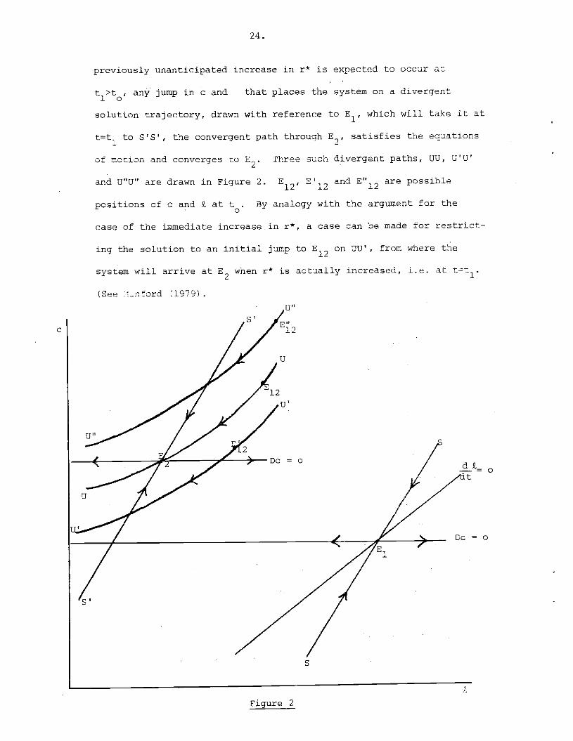
unstable and one stable root. Figure 2 depicts the response of c and

£ to an unanticipated permanent increase in r*. Thea =o locus coulddt

be downward—sloping, but nothing essential hinges on that. With both

c and £ free to jump in response to "news", the condition that c and 9.

remain bounded for bounded values of the exogenous variablesji and. r*

no longer suffices to select a unique solution trajectory. Consider

an immediate unanticipated increase in r* at ttt. The new long run

equilibrium is E2. The initial position at t is assumed to beE1.

Any jump in 2. and c which places the system anywhere on S'st at tt

satisfies the equations of motion and guarantees convergence to£2.

A plausible further restriction might be that the behaviour of this

system with its two "forward—looking" variables should not be depend-

ent on an "irrelevant" past. With the increase in r* occurring at

t, when it is first anticipated, this would mean that the system

jumps immediately to 2' the new long—run equilibrium. If a

C

24.

previously unanticipated increase in r* is expected to occur at

t1>t, any jump in c and that places the system on a divergent

solution trajectory, drawn with reference to E1, which will take it at

t=t1 to 5!5l the convergent path through E2, satisfies the equations

ci motion and converges no E2. Three such divergent paths, UtJ, GU'

and U"U" are drawn in Figure 2. E12, E'12 and E"12 are possible

positions of c and 9 at to. By analogy with the argument for the

case of the immediate increase.in r*, a case can be made for restrict-

ing the solution to an initial jump to E1.7 on UU', from where the

system will arrive at when r* is actually increased, i.e. at tt1.

(See :.nord (1979)

Figure 2

Ct

Dc

(3"

U'

U

Dc = 0

S

S

25.

The proposed boundary conditions therefore take the form:

-

_r(1—) (1-a(l+y)6k)+6tA(t1) A(1-cz(1+y)

(3 ) — —

c(t1) -

-i-a(i÷fl)

xrA(l—a(1+y$fl+Ay+ky(1-)

A(1—a(l+yt))

0— l—a(1+fl)

This class of boundary value problen can be solved using the method of

ad jointsThe method of adjoints

We consider the model of equations (3a,b) over a time interval

ttt1 during which the information set does not change, i.e.

I(t)=I. t tt1. Over this interval; therefore,3x2(s,t)

=0s=t

dx2(t) and equations (3a,b) or (7) can be written as:dt

(37) dx(t)Ax(t)-J.3z(t). t ttC

We now consider the two—point boundary value problem of equations (37)

and (38)

(38) Mx(t )+tx(t )=r0 1

Equation (38) gives n linear restrictions on the value of the state

vector at two distinct dates.

26.

Let M {p.} , N {v.,} and r = (p p

i,j=1, 2, ...,n.

We can therefore rewrite (36) as (33 l)

n n

(38') E .i.. xjt ) + E v., x.(t ) = p. j = 1, 2, ..., nJi 1 0 . J1 1 1 jt=l

x. now denotes the th elements of x , I = 1, 2, ..., n

Consider the adjoint system to (37)

(39) ds(t) = — AT s(t)

at

We integrate the adjoint equations backward from t = t1 , once for

each ,c,(t1) in (38 ') , using as the terminal boundary conditions

• (40) (J) (t1) = v,. I, j = 1, 2, ..., n

(ti)is the th component at t = t1 for the th backward integration

of the adjoint equation. Thus, if denotes the transpose of the

row of N in equation (38), we have the solution

_(t_t1)AT T(41) s(t) = e j = 1, 2

Setting t = to in (41) we obtain

The fundamental identity for the method of adjoints is (see Roberts and

Shipman 11972, pp. 17—221):

n . n . t n(42) £ (t ) x. (t ) - E s2x. (t = (t) b.z(t)dt

i=1' 1 ilt0=i

a. 1

j = 1, 2, . ., nb, is the

.throw of the matrix B

27.

Substituting for s (ti) from (40) into (42) and using (33') yields

n n t np. - E p.. x.(t) - I 5(t ) x(t ) I s(t)b.z(t)dt-, Ji 1 0 1 0 1 - 1 1i=1 1=! - t t=1

0

j = 1, 2, . . . , nor

tn in(43) I [p.. + st )] x.(t ) = p. -5 1 s9(t) .z(t)dt

i=l Ji 1. 0 1t i=i 3. 1

C= 1, 2 n

Equation (43). constitutes a set of n equations in the n unknowns

x(t) , i = 1, 2..., n. If they are linearly independent they will

yield a unique solution for x(t) . Given the value of the entire

state vector at t = to, equation (37) can be solved as a standard

initial value problem. Its solution would be

(43) x(t)=et_to)x(t)+feMt_5)Bz(s)ds, ttt1

However, in practical (i.e. numerical) applications, the true

value of x at t=t can only be approximated. Since A will in general

possess unstable characteristic roots, any error in the calculation

of x(t) will be compounded as time passes. If there are unstable

roots, it is therefore computationally superior, having calculated

x(t) using the method of adjoints, to use the solution method of

equations (17) or (17') and (23) or (23'). Note that z (T,s)z(r,t)

z(s) for tcst1 when we apply this method. If the information set

changes at t=t1, we resolve the two—point boundary value problem.

Equation (36) can be seen to be the special case of equation (38) with

M0.

2.8.

(4) CONCLUSiON

The paper presents a general solution method for rational expect-

ations models that can be represented by systems of deterministic

first order linear differential equations with constant coefficients.

It is the continuous time adaptation of the method of Blanchard and

Kahn; To obtain a unipie solution there must be as many linearly

independent boundary conditions as there are linearly independent

state variables. Three slightly different versions of a well—known

small open economy macroeconomic model were used to illustrate ttree

fairly general ways of specifying the required boundary conditions.

The first represents the standard case in which the number of stable

characteristic roots equals the number of predetermined variables.

The second represents the case where the number of stable roots

exceeds the number of predetermined variables but equals the number

of predetermined variables plus the number of "backward—looking" but

non—predetermined variables whose discontinuities are linear functions

of the discontinuities in the forward-looking variables The third

represents the case where the number of unstable roots is less than

the number of forward-looking state variables. For the last case,

boundary conditions are suggested that involve linear restrictions

on the values of the state variables at a future date.

The method of this paper permits the numerical solution of

models with large numbers of state variables. Any combination of

anticipated or unanticipated, current or future and permanent or

transitory shocks can be analysed.

29.

Acknowledgement footnote:

I would like to thank Marcus Miller, Stephen Turnovsky and

other members of the University of Warwick 1981 Summer Workshop for

helpful comments and suggestions. Financial support from the

Leverhultne Trust is gratefully acknowledged.

REFERENCES

Elanchard, 0. J. (1980) , "The Monetary Mechanism in the Light ofRational Expectations", in S. Fischer ed. Rational Expectationsand Economic Policy, University of Chicago Press, Chicago,pp. 75—116.

Blanchard, 0. J. and Kahn, C. M. (1980), "The Solution of Linear

Difference Models under RationalExpectations', Econometrica,

48, July, pp. 1305—1311.

Brock, William A. (1975) , "A Simple Perfect Foresight MonetaryModel", Journal of Monetary Economics 1, April, pp. 133-150.

Buiter, W. and Miller, Fl. (l9Sla), "Monetary Policy and International

Competitiveness: The Problems of Adjusaient", Oxford EconomicsPapers, pp. 143—175.

Buiter, W. H. and Miller, M, (198th), "Real Exchange Rate Overshooting

and the Output Cost of Bringing Down Inflation'. Forthcoming,European Economic Review.

Calvo, 0. A. (1977), "The Stability of Models of Money and PerfectForesight: A Comment", Econometrica, 45, October, pp. 1737—1939.

Dixit, A. (1980) , "A Solution Technique for Rational ExpectationsModels with Applications to Exchange Rate and Interest RateDetermination", Mimeo, University of Warwick, November,

30.

Dornbusch, a. (1976) , 'Expectations and Exchange Rate Dynamics",Journal of Political Economy, 84, December, pp. 1161-1176.

Dornbusch, R. and Fischer, S. (1980), "Exchange Rates and theCurrent Account', American Economic Review, 70, No. 5, December

Flood, a. and Garber, P. (1980) , "Market Fundamentals versus pricelevel bubbles: The first tests', Journal of Political Economy,

88, August, pp. 745—770.

Krugnan, p. (1979), "A Model of Balance of Payments Crises", Journalof Money, Credit and Banking, Il, August, pp. 311—325.

Minford, A. P. L. (1979) , "Terminal Conditions, Uniqueness and theSolution of Rational Expectations Models", Unpublished,

University of Liverpool.

Roberts, S. M. and Shipman, J. S. (1972) , Two-Point Boundary ValueProblems: Shooting Methods Elsevier, New York.

Sargent. T. and Wallace, N. (1973), "The Stability of Models cf Moneyand Growth with Perfect Foresight", Econometrica, 41,

Turnovsky, S. J. and Burmeister, E. (1977), "Perfect Foresight,

Expectational Consistency, and Macroeconomic Equilibrium",Journal of Political Economy, 85, April, pp. 379-393.

Wilson, C. (1979, "Anticipated Shocks and Exchange Rate Dynamics,"Journal of Political Economy, 87, June, pp. 636-647.

FOOTNOTES

(1) See Brock (1975) for a model in which these transversa24ty conditionsafe derived from explicit optimizing behaviour by an infinite—livedconsumer. The non—predetermined variables there have the intçtpret-ation of co-state variables in a dynamic optimization problem.

(2) The non-predetermined variables frequently are asset prices deter-mined in efficient asset markets. Implicit arbitrage conditionsrule out anticipated future jumps in these asset prices. Thus,except at those instants at which new information arrives, the non—predetermined variables are continuous functions of time. See Calvo(1977)

3]-.

(3) We do not howover, for reasons of space, consider solutions in which"extraneous' information plays•á role.

(4) The exponential matrix cC where C is an nxm matrix is defined by

C ke E I C When C is a diagonal matrixk—o k

_c. C1 1e 0

C c. C_1 thenez e0.• 0 . cU

c Cfl

(5) Using 11 l[ 11] =

(6) For any matrix S, denotes the (complex conjugate) transpose of s2.