An Alternative Interpretation of the ‘Resource Curse’: Theory and Policy ImplicationsRicardo Hausmann and Robert RigobonNBER Working Paper No. 9424December 2002JEL No. F0

ABSTRACT

The existence of a natural resource curse has been a longstanding theme in the economicliterature and in policy discussions. We propose an alternative mechanism and study its policyimplications. The mechanism is based on the interaction between two building blocks: specializationin non-tradables and financial market imperfections. We show that if a country has a sufficientlylarge non-resource tradable sector, relative prices can be stable, even when the resource sectorgenerates significant volatility in the demand for non-tradables. However, when the non-resourcetradable sector disappears, the economy becomes much more volatile, because shocks to the demandfor non-tradables - possibly associated with shocks to resource income - will not be accommodatedby movements in the allocation of labor but instead by expenditure-switching. This requires muchhigher relative price movements. The presence of bankruptcy costs makes interest rates dependenton relative price volatility. These two effects interact causing the economy to specialize inefficientlyaway from non-resource tradables: the less it produces of them, the greater the volatility of relativeprices, the higher the interest rate the sector faces, causing it to shrink even further until itdisappears. At that point, the economy will face an even higher interest rate and a lower level ofcapital and output in the non-tradable sector. An increase in resource income that leads tospecialization causes a large decline in welfare: thus the idea of the curse. Specialization isdetermined by the expected size and volatility in resource income. The paper justifies stabilizationand savings policies as well as policies to make financial markets more efficient. However, we alsofind some support for more interventionist second-best trade and financial

Ricardo Hausmann Roberto RigobonKennedy School of Government Sloan School of ManagementHarvard University MIT, E52-44779 JFK Street 50 Memorial DriveCambridge, MA 02138 Cambridge, MA 02142

and NBERrigobon@mit.edu

It is often said that most people when reading about a theory wonder if it works in

practice. Economists when they see things working in practice, wonder if they

work in theory. The natural resource curse is a case in point. Countries highly

dependent on oil or other natural resources performed very poorly since 1980.

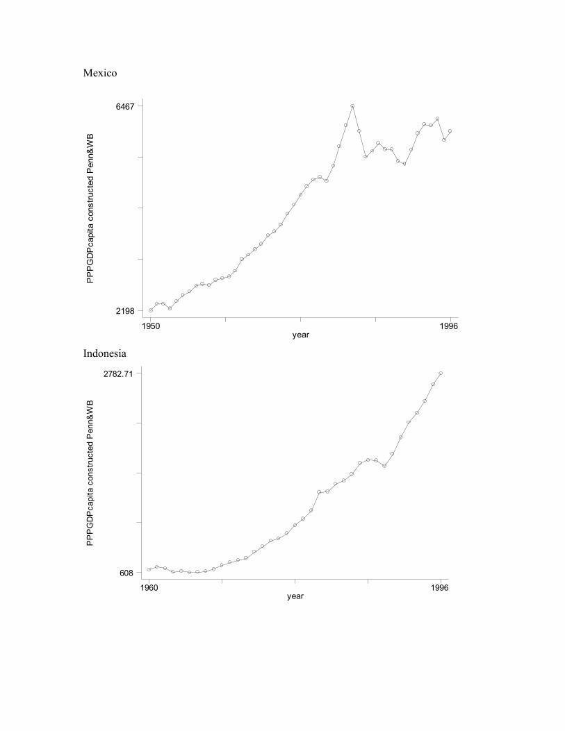
Figure 1 shows GDP per capita at purchasing power parity for highly resource-

intensive countries such as Saudi Arabia, Nigeria, Venezuela and Zaire, and for

less intensive countries such as Indonesia and Mexico. The pattern is clear, the

more dependent performed remarkably poorly. The less oil-dependent did better.

The concern that natural resource wealth may somehow be inmiserating is a

recurring theme in both policy discussions and in empirical analysis. The

empirical regularity seems to be in the data1 but understanding its causes has been

a much harder task2. Theorists have been hard at work to find a rationale. Is it a

consequence of the Dutch Disease? Is it caused by the volatility that characterizes

resource-based commodity prices? Is it due to political economy forces unleashed

by the presence of rents? And what are the policy implications of this problem?

1 For example, Sachs and Warner (1995) estimated that countries fully dependent on the export of

primary products grew about 2.5 percent per year more slowly in the 1970-1989 period. Gavin and

Hausmann (1998) and Higgins and Williamson (1999) find a strong relationship between resource

intensity and inequality.

2 For example, Manzano and Rigobon (2001) attribute the low growth to a debt overhang

associated with over borrowing during the boom of the 1970s.

1

Is there such a thing as having too much oil for the country’s own good? Should

oil income be saved in net terms? Or is the question mainly that of dealing with

the volatility in the flows? Are other policies called for?

In this paper we will propose an alternative rationale for the resource curse and

discuss some of its policy implications. The approach is based on the interaction

between two building blocks: specialization of the domestic economy in the

production of non-tradables and financial market imperfections. We show that as

an oil economy becomes more specialized in the production of non-tradables, the

real exchange rate becomes more volatile because shocks to the demand for non-

tradables –associated for example with the fiscal expenditure of shocks to

resource income – will not be accommodated by movements in the allocation of

capital and labor but instead by expenditure-switching. This requires much larger

relative price movements. Financial frictions such as risk aversion or costly

bankruptcy on corporate debt implies that the interest rate will be a function of the

volatility in the economy. In fact, the volatility of profits in the non-resource

tradable sector can be shown to be larger than in the non-tradable sector. As

volatility increases, sector-specific interest rates rise causing a decline in the

output that is larger for the non-resource tradable sector. A multiplier process is

set in motion where an initial rise in interest rates causes the tradable sector to

contract, further raising volatility and interest rates until the sector disappears. At

2

that point, the economy will face an even higher interest rate and a lower level of

capital and output in the non-tradable sector. An increase in resource income that

leads to specialization causes a large decline in welfare: thus the idea of the curse.

This form of specialization is inefficient and is characterized by high volatility

and interest rates, weak real exchange rates, low wages and investment.

Inefficient specialization is determined by the level and the volatility of resource

income and by the international interest rate. The paper discusses the role of fiscal

saving of oil revenues as well as stabilization of expenditures. In addition,

independent policies that reduce country risk and that improve the functioning of

financial markets are seen as being particularly important in this context. More

interventionist policies to subsidize investment in the non-resource tradable sector

may also have a role to play.

The paper is organized as follows. Section 1 summarizes and criticizes the

previous literature on the resource curse. It also presents the logic of our approach

in informal terms. Section 3 presents the formal model and analyzes its properties.

Section 4 discusses the policy implications..

I. Previous approaches to the resource curse

There have been several approaches in the literature to account for the resource

curse. The first is associated with the notion of the Dutch Disease. The second has

3

to do with the rent-seeking activities generated around the presence of the

associated tax revenue. The third approach has to do with the damaging effects of

volatility. In this section we will discuss each of these theories and their

limitations.

A. The Dutch Disease Approach

Increases in resource-based revenues, such as oil, generate a greater capacity to

import tradables, but typically prompt a greater demand for all goods including

non-tradables, which cannot be imported but must be produced locally. This

requires the economy to move resources out of the non-resource tradable sector –

call it manufacturing – in order to expand the production of non-tradables such as

construction and services. An oil boom would lead to a contraction in

manufacturing. A real appreciation is the mechanism that gets the job done

(Corden, 1982, Corden and Neary, 1984). This is the Dutch disease.

This logic is compelling, but by itself it does not imply any inefficiency or

welfare loss. It only states that booms in resource income would be associated

with contractions in manufacturing, not in overall growth. It cannot explain why a

country would grow more slowly, just because it has oil.

To get some mileage, one has to assume that non-resource tradables play a special

role in the growth process. This is the tradition started by Matsuyama (1992)

4

where he assumed that there are increasing returns to scale in manufacturing, but

not in the resource sector. Hence, an abundance of the natural resource makes the

economy specialize in the less dynamic sector3. Hence, this may explain the

curse.

One problem with this explanation is that one should expect that over the long run

oil-exporting countries would be doing poorly when oil is doing well and that

they would be improving when oil becomes less dynamic. However, over the 60

year period between the early 20s and the early 80s Venezuela was the country

with the highest growth in per capita income out of the 40 countries for which

Maddison (1992) has data. During the following 20 years, Venezuela is among

the worst performers in the world, a period which coincides with the decline of its

oil income (Hausmann, 2002). This is not just a coincidence. The same pattern

can be observed if we look at the growth rate of a wider group of countries over a

shorter period. As Table 1 shows, oil-exporting countries grew faster in the period

of rising oil prices and volumes between 1960 and 1980 relative to other

developing countries and collapsed when oil revenues declined after 1980. If the

Dutch Disease story was right, the post-1980 story should have been one of

greater growth. Hence, the story as such does not fit the facts.

3 Alternatively, it may want to diversify into resource-intensive industrialization, which has failed

in many countries, Auty (1990)

5

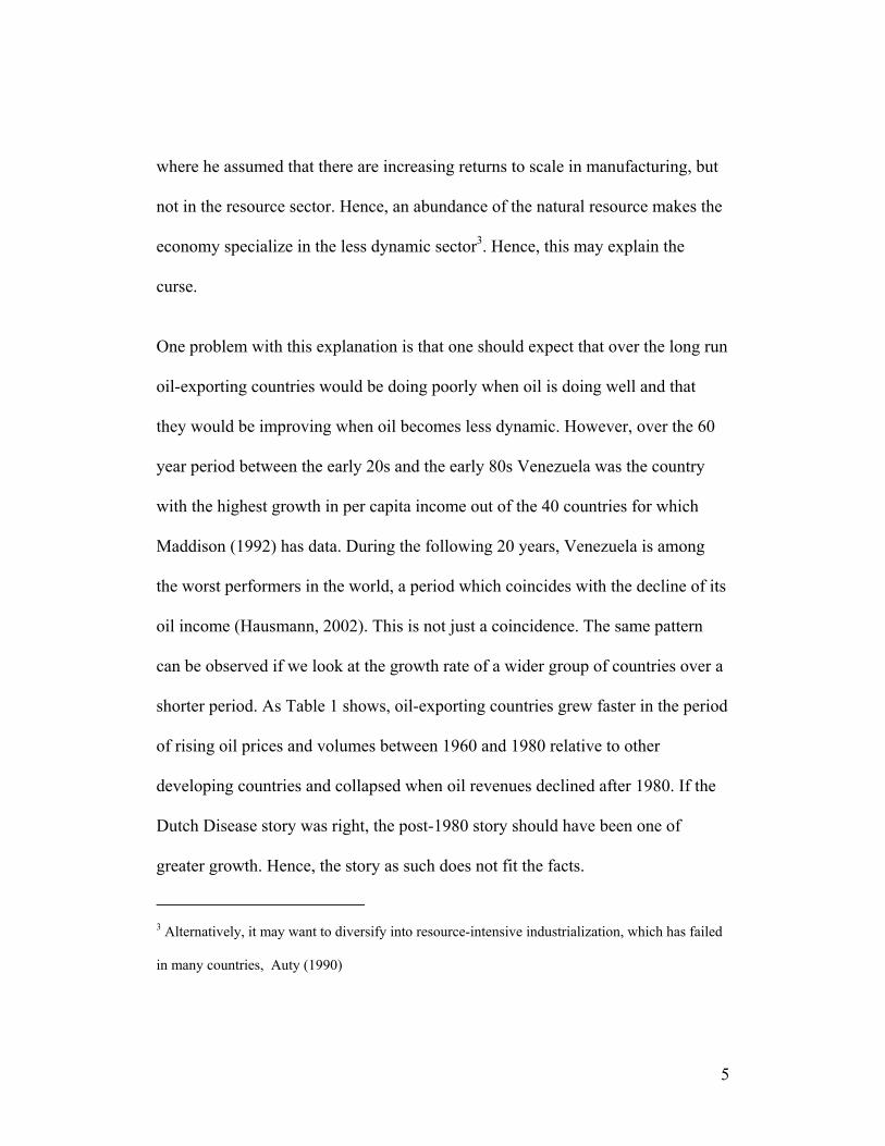
Table 1. Average annual growth in per capita GDP at purchasing power prices

Country group 1960-1998 1960-1980 1980-1998 Number of

countries

All developing 1.7 3 0.2 115

- oil exporters 1.1 5.2 -2.1 15

- others 1.8 2.7 0.5 100 Source: World Penn Tables, own calculations

Moreover, it is not obvious that learning by doing or technological development is

slower in resource based industries relative to others. As the World Bank (2001)

has shown in a recent report, several industrial countries such as Australia,

Canada and Finland became rich by developing the technology and capital goods

industries associated with their resource sectors. Moreover, whatever bad effects

specializing in natural resources might generate they have to be compared with

the benefits of owning large natural resources.

For example, natural resource income may raise national savings and hence

facilitate capital accumulation and growth. This is not a minor aspect as oil

exporting economies have averaged twice the savings rate of non-oil exporters

(Table 2). Moreover, they were able to save more and grow more in the period

when oil was growing fast (1960-1980) relative to the more recent episode (1980-

1998).

6

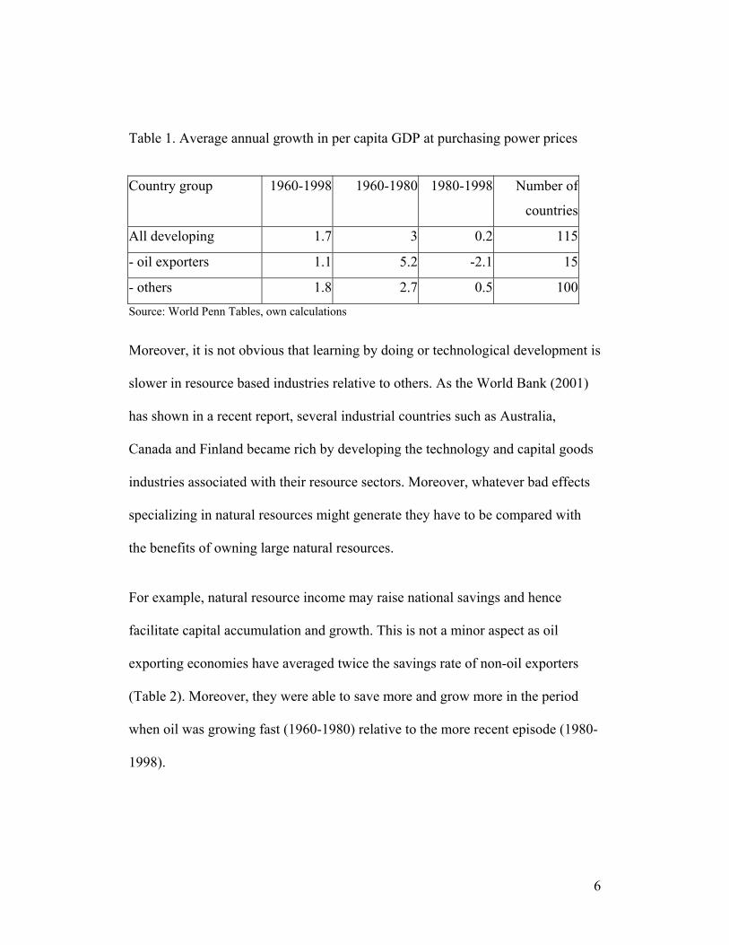
Table 2. Average domestic savings rate

Country

group

1960-1998 1960-1980 1980-1998 Number of

countries

All

developing

17.1 18.4 16.2 111

- oil

exporters

33.2 37.9 30.1 15

- others 14.6 15.3 14 96 Source: World Penn Tables, own calculations

B. The Rent-Seeking Story

An alternative story is that resource wealth such as oil somehow makes societies

less entrepreneurial. There is so much wealth floating around the government that

entrepreneurial persons find it much more profitable to engage in unproductive

rent-seeking activities to appropriate that wealth rather than in creating more

wealth. The presence of common-pool problems or uncertainty over property

rights over the resource income may generate low growth by inefficiently

focusing economies in fighting over existing resources.

The common-pool problem – caused by situations where costs are shared between

many agents but benefits are private (e.g. as in fiscal policy) – may lead to

overspending on average and to a distorted allocation of spending over time.

Overspending is associated with the idea that different constituencies do not

7

internalize the full cost of their spending requests, as they only pay a small

fraction of the additional tax burden. (Weingast, Shepsle and Johnsen, 1981, von

Hagen and Harden, 1994). This problem is not specific to resource rich

economies, but instead is present in all countries. However, in resource rich

economies, where non-resource taxes are typically low and resource rents are

large, it could be argued that this force could in theory be more powerful.

In a dynamic setting this logic may lead to overborrowing and to a voracity effect

(Hausmann, Powell and Rigobon , 1990, Velasco, 1995, Lane and Tornell , 1999).

Assume that it is best to save a temporary boom until some future time when

lower resource income is expected. An individual would choose to smooth

consumption. However, when there is a common-pool problem each constituency

will ask for a larger share of the pie in good times, fearing that if they don’t, other

constituencies might take it away.

This story again does not explain why oil economies did so well when incomes

were rising and why they have under performed so strongly in the last two

decades.

In yet a different setting, others have argued (Karl 1997) that oil economies, by

not developing the political compact that allows the State to tax its citizens are

8

poorly equipped to deal with collapses in oil revenues without leading to

macroeconomic crises.

This logic may be present, but other factors may well overwhelm it. We already

mentioned the fact that resource revenue may allow for higher savings. It may

also allow the country to reduce taxation over more mobile factors and hence

achieve a less distortionary overall taxation scheme, thus generating a more

propitious economic environment for growth. Moreover, the political skills

required to allocate rents among different groups may be useful in achieving the

necessary reallocations when income declines.

C. The volatility story

An alternative explanation to the curse puts the emphasis on volatility. Volatility

has been shown to be bad for growth, for investment, for income distribution, for

poverty and for educational attainment4. Natural resource rents tend to be very

volatile because the supply of natural resources exhibits low price-elasticities of

supply. For example, the standard deviation of oil price changes has been about

30 to 35 percent per year. For a country where oil represents about 20 percent of

4 See IDB (1995), Gavin and Hausmann (1996), Ramey and Ramey (1995), Aizenman and Marion

(1999), Caballero (2000). Flug et al (1996) and Duryea (1998) discuss the impact of volatility on

educational attainment.

9

GDP, a 1 standard deviation shock to the price of oil represents an income shock

equivalent to 6 percent of GDP. This is huge relative to total GDP volatilities in

industrial countries (about 2 percent) or even developing countries (between 3 and

4 percent).

But how does volatility in the terms of trade damage the economy? Assume that

resource revenues are distributed to the population as a whole, say through

government transfers. This means that the fact that the revenue is volatile makes it

less valuable to risk-averse consumers. Let us take a relatively severe example.

Assume that in a given economy oil is 30 percent of national income and that it

has a standard deviation of about 30 percent per year. Assume that utility can be

described with a constant relative risk aversion (CRRA) utility function with a

relatively high coefficient of risk aversion of 3. This implies that consumers

would be willing to sacrifice 4.05 percent of national income in order to make oil

revenues perfectly certain. They would be willing to spend that much money in

hedging their resource risk: certainly more than a simple nuisance, but nothing

that could reasonably be called a curse, when compared with the revenue it

generates. This could reasonably justify organizing a seminar to discuss how

governments should manage this risk, but is not an adequate explanation for the

massive collapse in growth exhibited in Figure 1.

10

So the welfare losses associated with the consumption risk of the flow itself are

not particularly large. To get bigger effects, the rest of the economy must

somehow be disrupted by the volatility in oil. Interestingly, in a neo-classical

setting, it is quite hard to make volatility matter. Imagine first a competitive

economy in which capital is perfectly mobile internationally and labor is

nationally fixed, but is perfectly mobile domestically across sectors. Assume that

there are three sectors: a resource sector – which we will call oil; a tradable sector

and a non-tradable sector. Oil is produced without either capital or labor: it is like

manna from heaven. One can also think of it as aid. The two other sectors are

produced with capital and labor and exhibit constant returns to scale. In this case,

so long as all goods are produced domestically, the volatility of the oil sector will

not affect the value of non-oil output or any non-oil relative price. The income of

workers and the rate of return to capital in the non-oil economy will be unaffected

by oil volatility!. Hence, the only problem will be the dislike for oil volatility

itself and this we have already found not to be too serious.

To understand this surprising result it is important to remember that there are five

prices in this economy. First, the price of oil is determined abroad. Second, the

rate of return to capital will be set by the world interest rate, given perfect capital

mobility. Third, the price of tradables will be set internationally through the law

of one price. Fourth, the internationally determined price of tradables and cost of

11

capital together with the zero-profit condition required by perfect competition will

set the wage that the tradable sector can pay, which will determine, through the

free movement of workers between sectors, the wage rate for the whole economy.

Fifth, this will determine non-tradable prices since wages and the cost of capital

are already set and profits must be zero. Shocks to the demand of non-tradables

(induced possibly by oil shocks) will be adjusted through movements of labor

between sectors and movements of capital in and out of the economy. The

production possibility frontier will be completely flat as shown in Figure 2.

We find this to be a very important benchmark not because it is an adequate

description of the world, but because it provides a point of departure to think of

the possible characteristics of the world – not included in the benchmark - that

may explain why oil and its volatility may become really problematic.

With full employment, and set wages and returns to capital, non-oil income will

be stable. The only source of volatility will be the direct impact of oil revenues in

household income. As we mentioned above, the welfare losses associated with

this uncertainty are not huge: a nuisance more than a curse. To get to explain a

curse the non-oil economy must be more seriously disturbed by oil volatility.

What features of the world does our benchmark not take into account? First,

capital takes time to build and once invested is usually irreversible. It cannot

12

move instantaneously between sectors. This is certainly a problem. It means that

the production function will be convex and that the volatility on government

spending will cause shifts in relative prices. However, the consequences of this

are not as serious as one might think. In a standard model, profits are a convex

function of relative prices (Caballero 1991). This means that the greater the

volatility in relative prices the larger will be the expected profits and average

investment! Moreover, if we assume full employment, the welfare of workers

may actually go up and not down with volatility, since they would be working on

average with more capital. Hence, irreversibility of investment cannot be the basis

for a serious curse.

Second, consider the presence of price and wage rigidities that prevent the labor

market from clearing. In this case, and assuming that capital is pre-determined

and irreversible5, volatility in oil income and government spending will translate

into changes in unemployment and output in the non-tradable sector. Notice,

however, that the tradable sector will remain unaffected: it will face constant

prices, wages and stock of capital. Therefore employment and output will be

constant. The non-tradable sector will have constant capital and wages but volatile

output. It will also have more capital invested in the non-tradable sector than in

5 In makes sense to assume that if prices cannot be readjusted, that capital should be even harder to

adjust.

13

our benchmark, given the convexity of the profit function. Welfare losses caused

by oil volatility are likely to be larger, because volatility is larger, but the

expected average levels of output and consumption should not be much affected.

D. Our approach

So where can the curse come from? We will argue that it will arise from an

interaction between specialization and financial market imperfections. In the

benchmark model we assumed that the economy was producing all goods. What

happens if the non-oil economy stops producing tradables and becomes

completely specialized in non-tradables? Central to the results of the benchmark

model is the requirement that there be a positive level of production of tradables:

the non-oil economy must not be fully specialized in non-tradables. This allows

labor movements between sectors to absorb the shocks to non-tradable demand. If

the economy were fully specialized in non-tradables, this result would disappear

(Figure 3). Labor would now be fixed and fully employed in non-tradables. The

only way to expand supply would be by increasing the amount of capital per

worker in the sector. But capital is required to get the international rate of return.

However, with labor fixed, the productivity of each additional unit of capital

would be falling. To avoid returns to capital to fall, the price of non-tradables

must go up. Hence, the supply of non-tradables will now be upward sloping. But

the demand for non-tradables must be downward sloping. An increase in the price

14

of non-tradables will cause expenditure-switching effects, as consumers will

substitute away from the now more expensive non-tradables and into tradables.

The relative price between these two goods, i.e. the real exchange rate will have

to move in order to clear the market for non-tradables.

So, in our benchmark model, a specialized economy with volatile resource

revenue will see a volatile real exchange rate, while a diversified economy will

have a constant real exchange rate. In this setting, irreversibility in capital will

make relative prices even more volatile, as now the supply of non-tradables would

be completely pre-determined, given that both labor and capital will be fixed.

Only expenditure-switching forces will be at play. This will make the real

exchange rate even more volatile.

We will show below that this still is not enough to generate a real curse. In this

paper we will propose a form of financial imperfection that will cause interest

rates to be sensitive to the volatility in the real exchange rate. In particular, we

will assume that only debt contracts are available and that bankruptcy is costly.

This will make interest rates go up as the volatility of the real exchange rate

increases. There is a vicious circle between greater volatility and interests rates on

the one hand and lower investment in tradables on the other. The interest by the

tradable sector increases until the sector disappears and the economy specializes

inefficiently in non-tradables. The specialized economy will exhibit higher

15

interest rates on nonn-tradables, lower capital and wages and a more depreciated

exchange rate.

II. Modeling the curse

In this section we offer a formal model of the inefficient specialization. The

ingredients of the model are the following: Assume there are three sectors in the

economy, tradables, non-tradables and oil. Oil is assumed to consume no inputs

and generates a stochastic stream of revenues denominated in tradables. We

assume it is exogenous and denoted by Lg~ .

The tradable and non-tradable sector are comprised of a finite number of firms,

each using one unit of capital and producing output according to

α−= 1NN ly

in the non-tradable sector, and

α−= 1TT ly

in the tradable sector.

We assume that capital is owned by foreigners. This simplifies the analysis as it

allows us to disregard the effect of changes in capital income. Furthermore, the

16

results are unaffected (qualitatively speaking) by assuming that domestic agents

own some capital. We will assume that capital is irreversible and that it has to be

decided one period before production and oil revenues are realized.

We assume that oil belongs to the government, which consumes it entirely in non-

tradable goods. If the government decides to save its oil revenue, it will do so in

foreign assets. We will assume that households derive no utility out of

government consumption. This means that the volatile government consumption

will not enter directly into the utility of risk-averse households who might want to

smooth it. This eliminates the standard justification for stabilization. As discussed

above, this cannot possibly be the source of the curse if there is one. We assume

that there are no taxes.

Finally, we assume that capital is fully depreciated in one period and that

consumers cannot save. Thus, in this regard, the model is equivalent to a single

period model. Consumers have a standard Cobb-Douglas utility function, with

equal weights on tradable and non-tradable goods, and the share of non-tradables

is β.

17

1. Production

We assume that firms are small (price takers). We assume there are firms in

the non-tradable sector. Each firm requires an investment of one unit of capital to

operate, and each production function is given by

NN

α−= 1NN ly

Optimal labor decisions conditional on the capital invested in the non-tradable

sector solves

NNN wllP −−α1max

where and are the price of non-tradable goods and wages in domestic

currency respectively. The solution implies that labor demand is

NP w

( ) αα

1

1

−=

wP

l NN

production is

( ) αα

α−

−=

1

1wP

y NN

18

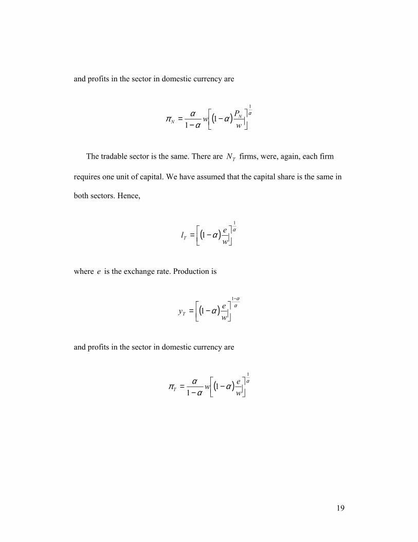
and profits in the sector in domestic currency are

( ) αα

ααπ

1

11

−

−=

wP

w NN

The tradable sector is the same. There are firms, were, again, each firm

requires one unit of capital. We have assumed that the capital share is the same in

both sectors. Hence,

TN

( ) αα

1

1

−=

welT

where e is the exchange rate. Production is

( ) αα

α−

−=

1

1weyT

and profits in the sector in domestic currency are

( ) αα

ααπ

1

11

−

−=

wewT

19

2. Government

We assume that oil exports are in dollars. Hence, the total government

consumption of non-tradable goods is

LgPe

N

~

In this simple setup we are assuming that the government does not face any

financial frictions. In other words, the cost of financing is the same as the benefits

of saving.

3. Demand

Households consume tradable and non-tradable goods, but not oil. There are no

taxes. We assume that consumers’ utility can be represented by the standard

Cobb-Douglas utility function. Furthermore, to simplify the number of parameters

under study, we assume that the weights are the same.

Assume the consumers solve

WCPeCstCC

NNT

NT

≤+

−

.max 1 ββ

20

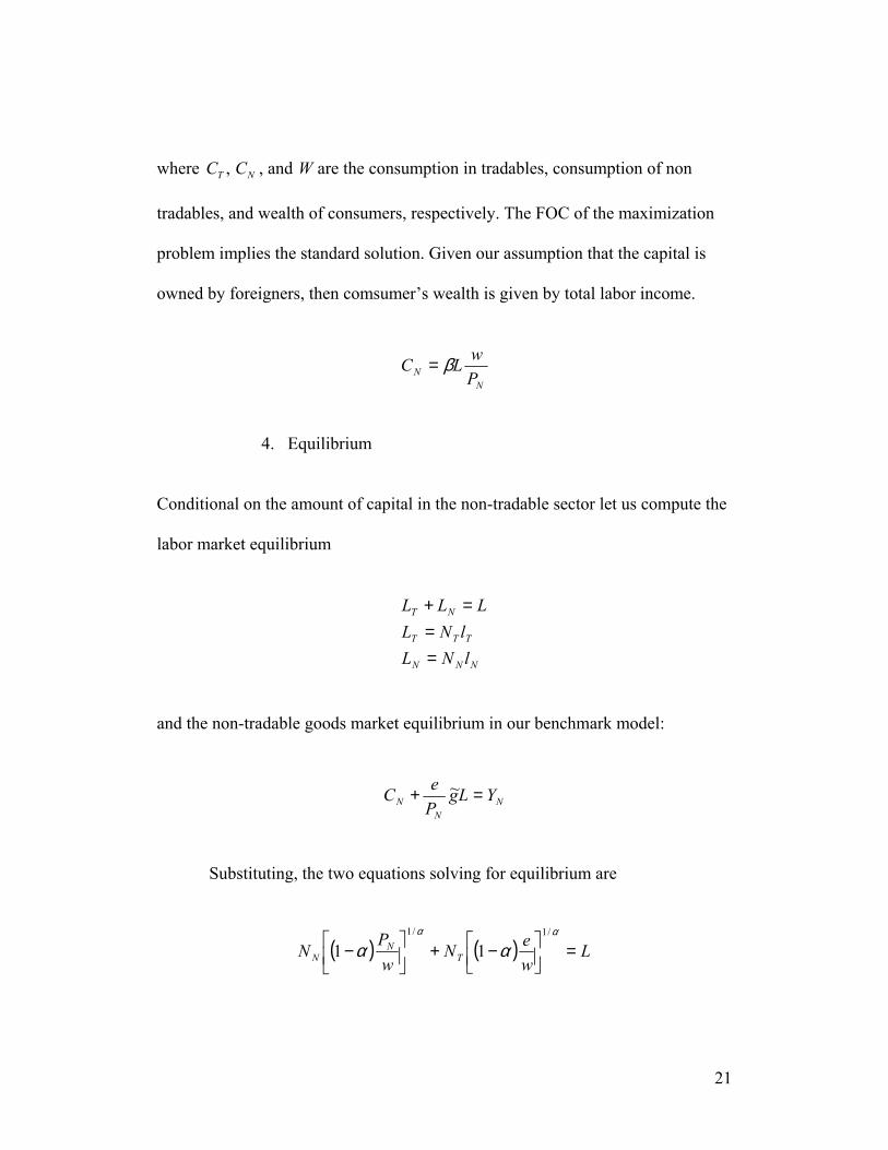
where C , and W are the consumption in tradables, consumption of non

tradables, and wealth of consumers, respectively. The FOC of the maximization

problem implies the standard solution. Given our assumption that the capital is

owned by foreigners, then comsumer’s wealth is given by total labor income.

NT C,

NN P

wLC β=

4. Equilibrium

Conditional on the amount of capital in the non-tradable sector let us compute the

labor market equilibrium

NNN

TTT

NT

lNLlNL

LLL

==

=+

and the non-tradable goods market equilibrium in our benchmark model:

NN

N YLgPeC =+ ~

Substituting, the two equations solving for equilibrium are

( ) ( ) LweN

wP

N TN

N =

−+

−

αα

αα/1/1

11

21

( ) αα

αβ−

−=+

1

1~wP

NLgPe

PwL N

NNN

Define,

N

N

PeQ

wP

q

=

=

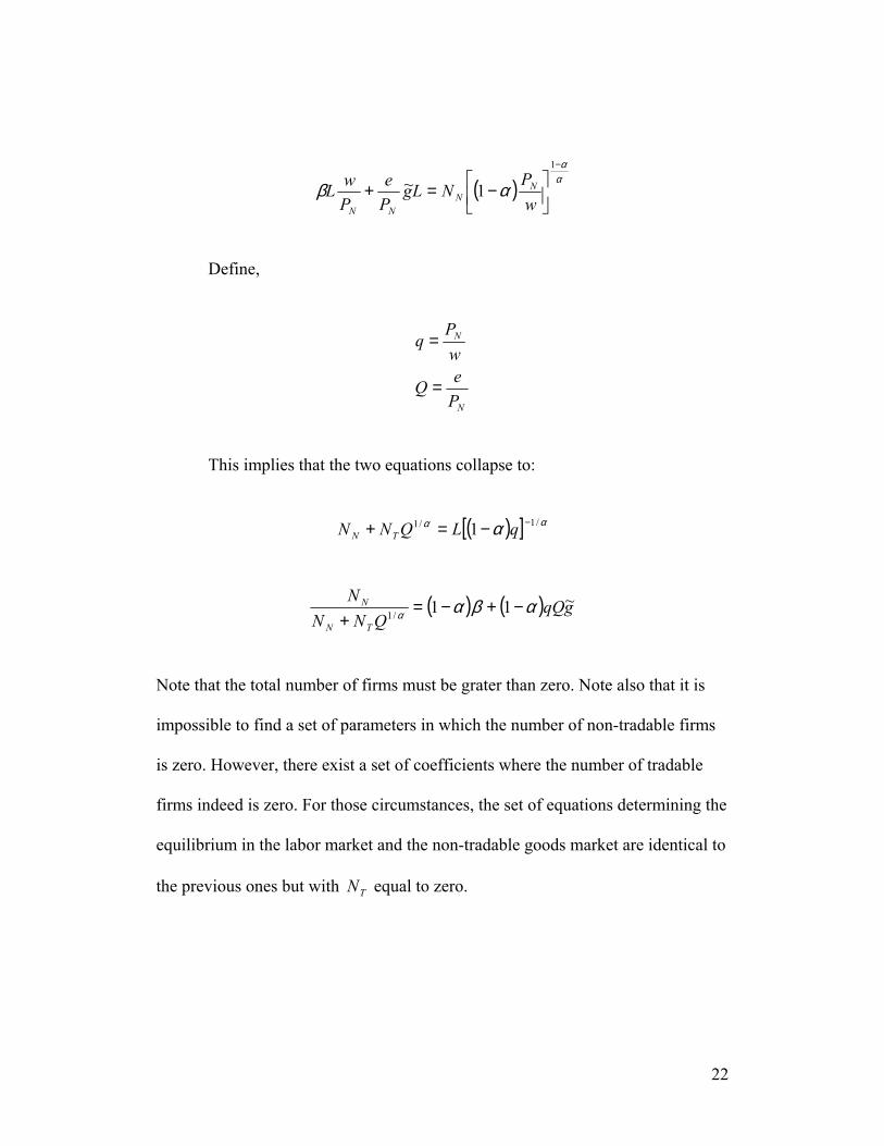
This implies that the two equations collapse to:

( )[ ] αα α /1/1 1 −−=+ qLQNN TN

( ) ( ) gqQQNN

N

TN

N ~11/1 αβαα −+−=+

Note that the total number of firms must be grater than zero. Note also that it is

impossible to find a set of parameters in which the number of non-tradable firms

is zero. However, there exist a set of coefficients where the number of tradable

firms indeed is zero. For those circumstances, the set of equations determining the

equilibrium in the labor market and the non-tradable goods market are identical to

the previous ones but with equal to zero. TN

22

After some algebra these two equations collapse to the following relationship

( )[ ]

α

αα

βα

/1

~11

QNNN

gL

N

TN

N

T

+=Ψ

Ψ=

Ψ−−−

Hence, assume the number of firms in the non-tradable sector is fixed, this

equation uniquely defines the solution for the number of tradable firms in

equilibrium. Lets study the equilibrium in Figure 4.

The downward slopping line corresponds to the LHS of the equation, and the

increasing concave schedule is the RHS. Notice that all the uncertainty of oil

expenditures appears on the RHS. Hence, we have depicted three schedules

reflecting the (supposedly) maximum, median and minimum of the shocks.

As can be seen, the two schedules determine (uniquely) the real exchange rate at

which both equilibrium conditions are satisfied. Note that for each realization of

the oil price there is a corresponding RER.

In the figure, we have depicted an increase in the number of tradable firms. This

makes the LHS line steeper. For a given level of uncertainty, this implies an

increase in the expected value of Ψ, and a reduction in its variance. Since Ψ is an

inverse function of the RER, we conclude that a larger tradable sector requires a

23

more depreciated exchange rate, but delivers a more stable RER for the same

degree of oil-related uncertainty.

This is an important characteristic of the model and it is useful to understand what

drives it. When the number of tradable firms is large (small), reductions in the

demand for non-tradables can be accommodated through an expansion in the

output of tradables with a relatively small (large) decline in the real wage, since

the high (low) stock of capital per potential worker invested in tradable

production implies that the marginal product of labor declines little (a lot) for

every additional worker. In the limit, if there is no capital invested in the tradable

sector, there will be no employment in the sector and the adjustment will take

place exclusively through the expenditure switching implications of real exchange

rate movements. This fact will become important below when we endogenize the

number of firms.

5. Irreversible Capital and Financial Frictions

The final ingredients of the model relate to the investment decision, which in this

setup is equivalent to the number of firms in each sector. As was mentioned

before, foreigners own the capital in both sectors. They have to decide the number

of firms that will operate in each sector before the government expenditure is

24

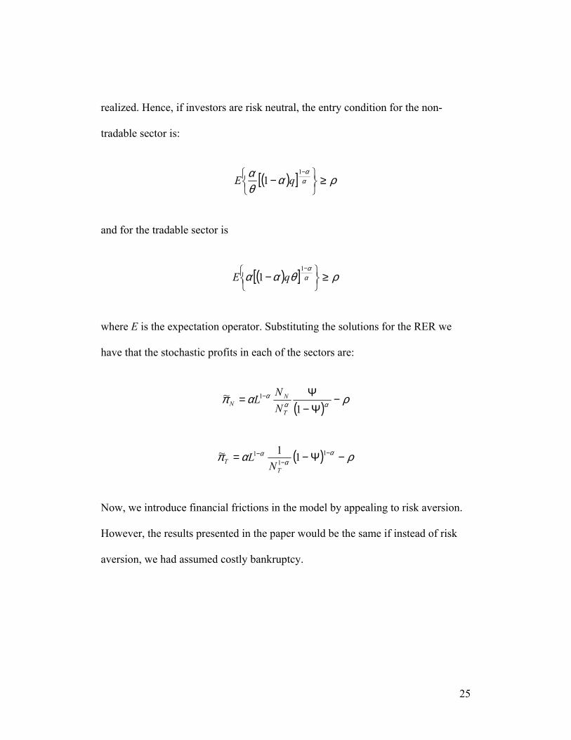
realized. Hence, if investors are risk neutral, the entry condition for the non-

tradable sector is:

( )[ ] ραθα

αα

≥

−

−11 qE

and for the tradable sector is

( )[ ] ρθαα αα

≥

−

−11 qE

where E is the expectation operator. Substituting the solutions for the RER we

have that the stochastic profits in each of the sectors are:

( )ραπ αα

α −Ψ−

Ψ= −

1~ 1

T

NN N

NL

( ) ραπ αα

α −Ψ−= −−

− 11

1 11~T

T NL

Now, we introduce financial frictions in the model by appealing to risk aversion.

However, the results presented in the paper would be the same if instead of risk

aversion, we had assumed costly bankruptcy.

25

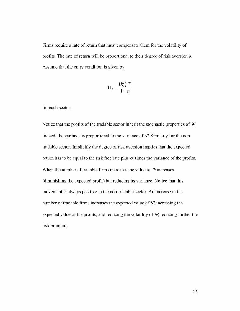
Firms require a rate of return that must compensate them for the volatility of

profits. The rate of return will be proportional to their degree of risk aversion σ.

Assume that the entry condition is given by

( )σ

π σ

−=Π

−

1

~ 1i

i

for each sector.

Notice that the profits of the tradable sector inherit the stochastic properties of Ψ.

Indeed, the variance is proportional to the variance of Ψ. Similarly for the non-

tradable sector. Implicitly the degree of risk aversion implies that the expected

return has to be equal to the risk free rate plus σ times the variance of the profits.

When the number of tradable firms increases the value of Ψ increases

(diminishing the expected profit) but reducing its variance. Notice that this

movement is always positive in the non-tradable sector. An increase in the

number of tradable firms increases the expected value of Ψ, increasing the

expected value of the profits, and reducing the volatility of Ψ, reducing further the

risk premium.

26

6. Simulation

In this section we simulate numerically the model in order to understand the

implications of changes in the size of the oil revenues, its volatility and degree of

risk aversion on the economy. In particular, we will study their effect on the

number of firms in each sector, the utility of households and the volatility of the

real exchange rate. The parameters chosen for the simulation are as follows. The

economy has a size of L=1. We assume that the rate of return required is equal to

5 percent. We set α equal to 0.25 and not the more common 0.3~0.4 because in

this model, capital is composed of tradable goods. In real life, capital also has

non-tradable components. However, assuming a demand for non-tradables for

investment purposes would have complicated the model unnecessarily.

We let the mean level of oil income move from 0.1 to 0.8. We assume that it is

uniformly distributed with a coefficient of variation of zero, 0.25, 0.75 and 0.875.

We present our results for two cases: a risk neutral case (σ=0, which we interpret

as no-financial frictions) and an alternative case with a relatively large degree of

risk aversion (σ=15).

In each figure the x-axis indicates the mean level of the oil income. Each figure

has four panels: the top panel is the number of non-tradable firms in equilibrium,

the second one is the number of tradable firms, the third is the utility of

27

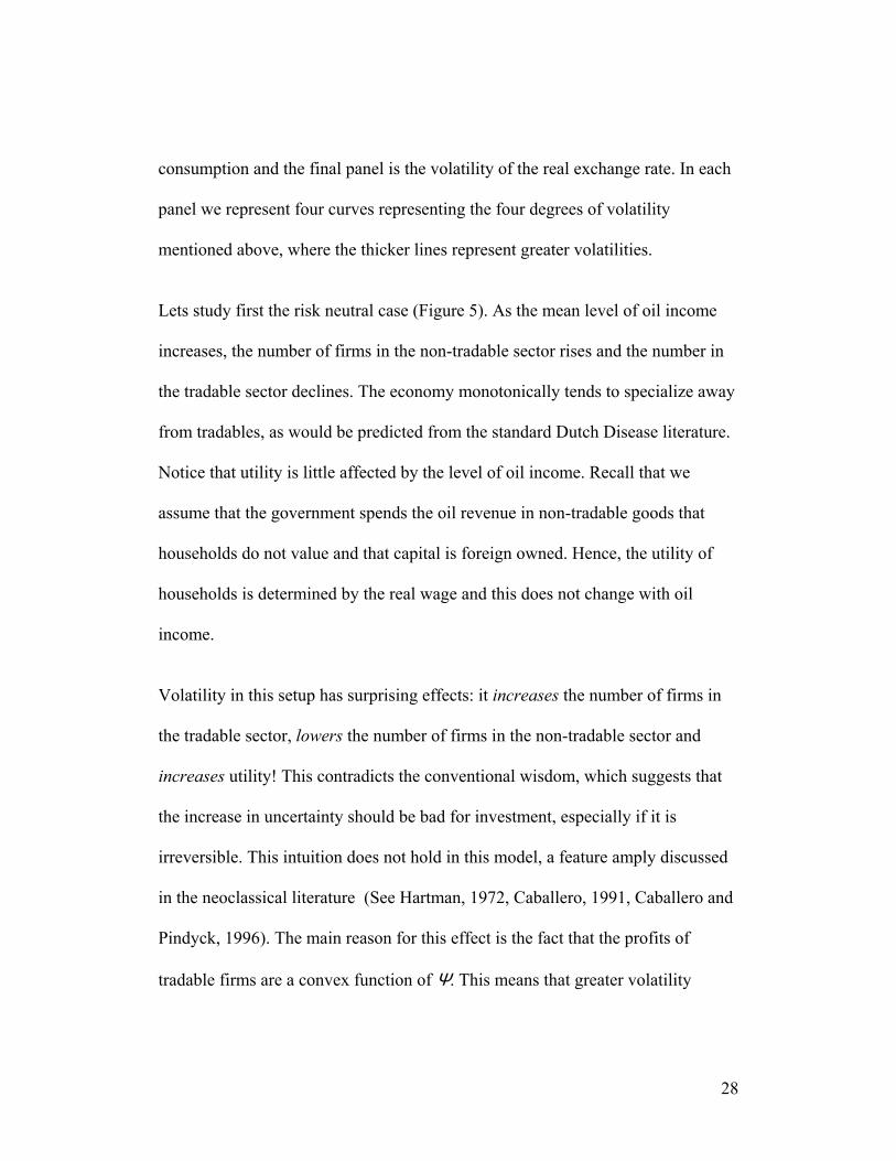
consumption and the final panel is the volatility of the real exchange rate. In each

panel we represent four curves representing the four degrees of volatility

mentioned above, where the thicker lines represent greater volatilities.

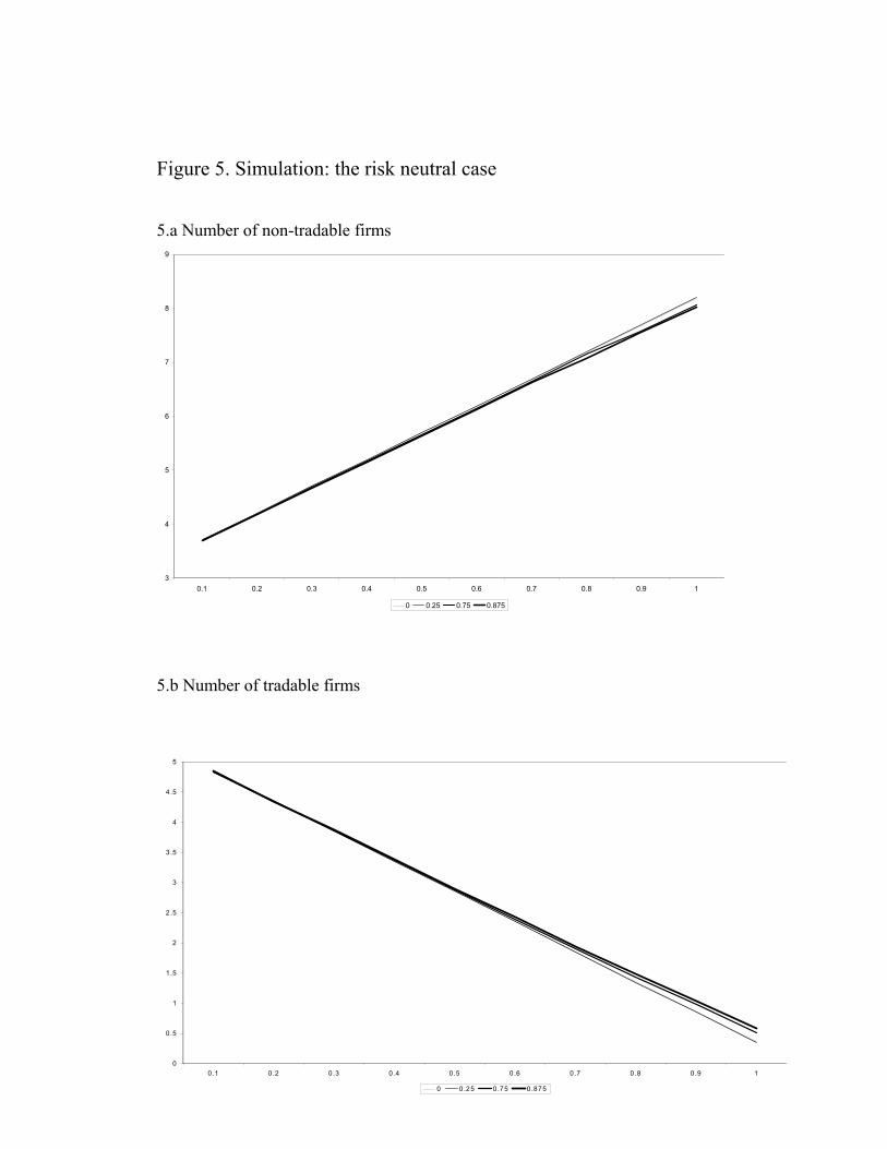
Lets study first the risk neutral case (Figure 5). As the mean level of oil income

increases, the number of firms in the non-tradable sector rises and the number in

the tradable sector declines. The economy monotonically tends to specialize away

from tradables, as would be predicted from the standard Dutch Disease literature.

Notice that utility is little affected by the level of oil income. Recall that we

assume that the government spends the oil revenue in non-tradable goods that

households do not value and that capital is foreign owned. Hence, the utility of

households is determined by the real wage and this does not change with oil

income.

Volatility in this setup has surprising effects: it increases the number of firms in

the tradable sector, lowers the number of firms in the non-tradable sector and

increases utility! This contradicts the conventional wisdom, which suggests that

the increase in uncertainty should be bad for investment, especially if it is

irreversible. This intuition does not hold in this model, a feature amply discussed

in the neoclassical literature (See Hartman, 1972, Caballero, 1991, Caballero and

Pindyck, 1996). The main reason for this effect is the fact that the profits of

tradable firms are a convex function of Ψ. This means that greater volatility

28

increases expected profits and investment in tradables. On the other hand, the

profits in the non-tradable sector can be concave or convex in Ψ and hence the

volatility will have less salutary effects. For the parameters in this model the

function is concave and the number of non-tradable firms falls with volatility6.

Utility increases because wages are also convex in Ψ. Interestingly, specialization

in this model is not associated with volatility but instead solely with the average

level of oil income. Hence, policies geared at stabilization are not welfare

improving.

We now turn to the case with risk aversion (Figure 6). We assume a level of risk

aversion of 15, which is high by conventional standards but significantly less than

the coefficient of 40 required to explain the equity premium in developed

countries. Remember that we take risk aversion to be a proxi for financial

frictions in the economy.

Here we observe a similar initial impact of increases in the mean level of oil

income on the number of firms in both sectors. However, notice that now

volatility lowers the number of firms in both sectors, as investors demand a higher

return to compensate for the greater variance in their returns, overwhelming the

6 In fact, for most reasonable set of parameters the schedule is concave. The relationship becomes

convex when the number of non-tradable firms approaches zero.

29

otherwise convex relationship of profits on Ψ. There is a point at which the

tradable sector completely shuts down. We refer to this phenomenon as inefficient

specialization. At that point, the number of firms in the non-tradable sector also

declines (and then rises very gradually), the volatility of the real exchange rate

increases by a factor of more than 10 and utility collapses.

The mechanism that brings this about is a vicious circle between specialization

and volatility. Remember that the volatility of the real exchange rate and Ψ is

inversely proportional to the number of firms in tradables. As the number declines

profits become more volatile, but risk aversion requires now a higher risk

premium, which lowers investment in tradables further and further increases

volatility. The sector disappears because the cost of capital makes expected firm

profits negative. This happens only in the tradable sector because its price is

exogenously set. In the non-tradable sector, the increase in risk premia lowers

investment, but this increases the price of non-tradables, preserving profitability.

The decline in utility is related to the magnitude of the inefficiency of the

specialization. A measure of this inefficiency is the difference between the

number of tradable firms in the zero volatility curve and the actual number of

firms. Notice that as the average level of oil income increases, the economy

would naturally specialize and hence the gap between the efficient number of

firms and the actual number declines. Hence, utility recovers, but does not reach

30

the no volatility level because the absence of the tradable sector makes the real

exchange rate more volatile and hence lowers the investment in non-tradables,

where the number of forms also falls relative to the optimal level.

This result might help explain why countries that were very specialized in oil

production such as Saudi Arabia, Nigeria and Venezuela fared so poorly when oil

income declined while countries such as Indonesia, Mexico and Norway were

much less affected. The first group was specialized in oil and when oil income

declined that specialization became much more inefficient, while the lack of a

tradable sector created a level of volatility and risk premia that did not allow for

investment. Diversified countries could adjust with much smaller costs.

In conclusion, (i) specialization in the production of non-tradables creates an

economy with more volatile relative prices. (ii) financial frictions interact with

this volatility further specializing the economy as the stock of capital will respond

to the greater macroeconomic volatility. (iii) this specialization may lead to the

complete and inefficient disappearance of tradable production. (iv) this

specialization reduces the investment in non-tradables - which will face a larger

cost of capital - and lowers welfare.

31

Clearly, in this context, a higher level of oil revenues can become a curse if it

leads the economy to inefficiently specialize. Moreover, stabilization policies can

have large welfare implications.

III. Policy implications

The curse of natural resources has so far been explained as being caused by either

rent-seeking or diversification away from sectors enjoying increasing returns.

Separately, expenditure stabilization policies have been advocated based on the

welfare benefits of consumption smoothing. In this paper we have proposed an

alternative mechanism for the curse that integrates it with the discussion of

stabilization.

We point out that an economy that is diversified, in terms of having a significant

non-oil tradable sector, will be much less affected by volatility in government

domestic spending than an economy that is already fully specialized in non-

tradables. This is so because in a diversified economy shocks to non-tradable

demand can be accommodated through changes in the structure of production

while specialized economies have to rely on expenditure switching. We note that

countries with more resource rents will naturally produce fewer tradables and

hence are more likely to be naturally specialized.

32

However, the presence of quite standard financial frictions, such as costly

bankruptcy, will make relative price volatility affect the cost of capital through

risk premia. This has three major consequences: first, it causes the economy to

specialize further by making it harder and in some cases impossible for the

tradable sector to access capital; second, it causes higher interest rate and less

capital in the non-tradable sector under specialization; third, it greatly increases

the welfare losses caused by volatility.

The policy implications of this model are relatively straightforward. They have to

do with avoiding inefficient specialization, and reducing the costs of volatility.

We separate our discussion in two parts. First we deal with first-best policies,

which are based on reducing the distortions in the economy. Then we move to

second-best policies, where we assume that the distortions are hard to remove and

look at interventions that can improve welfare, given that the distortions make the

market outcome inefficient. This is in general the spirit of the policies we are

discussing below.

A. Fiscal policy

To discuss fiscal policy it is important to separate between three types of

countries:

33

• Those that are naturally specialized, i.e. those that would specialize even

in the absence of volatility.

• Those that are inefficiently specialized

• Those that are not specialized and would like to stay that way

1. Naturally Specialized Countries

These countries have so much natural resource wealth that it does not make sense

for them to engage in the production of other tradables, even in a first-best world.

Some Gulf states might be in this category. However, in these countries,

specialization makes relative prices very sensitive to the volatility in government

spending. These countries would benefit from policies that stabilize government

expenditures in order not to transmit volatility to the domestic market.

2. Inefficiently Specialized Countries

These countries are suffering from major welfare losses associated with the

inability to develop the tradable sector, which makes the cost of capital high, even

for non-tradable sector. Countries such as Venezuela and Nigeria may be in this

category. Inefficient specialization is the product of a combination of factors: the

level of government spending, the volatility of that spending, the “commercial-

risk-free” interest rate to which firms in the economy have access and the

magnitude of financial inefficiencies.

34

These countries need to make a big effort to change the structure of the economy

sufficiently to get it over the specialization frontier. Incremental changes may not

be enough to improve matters significantly. There are three fiscal margins in

which these economies could work: the average level of government spending, its

volatility and the “commercial-risk-free” interest rate.

With respect to the first point, it is useful to be precise in what we call

“government spending” in the context of our model. We assumed that there was

no domestic taxation. In a world with taxes, the relevant policy variable is the

primary deficit excluding oil revenues and external spending by the government.

This variable must be credibly lowered and stabilized in order to cross the

specialization frontier. There is some trade-off between lowering the average and

lowering its volatility. The more credible the reduction in volatility, the less

important will be the required reduction in average spending. However, our

simulations suggest that, for the parameters we studied, feasible cuts in average

spending seem quantitatively more effective than feasible reductions in volatility,

although the latter bring greater improvements in welfare. Hence, an ideal policy

would rely on both. Hence, stabilization per se would not be enough: cuts in the

structural non-oil primary deficit would be called for.

Furthermore, fiscal policy and debt management policies have an important role

to play in affecting the interest rate. In our model we assumed a riskless

35

international interest rate to which we added the commercial risks faced by each

sector. In real life, on top of this commercial risk there may be country risk,

associated with fears about the sustainability of public debt and of the

government’s fiscal position. Factors that increase country risk will have the

effect of moving the specialization frontier in: the economy will specialize at

lower average levels of spending and at lower volatilities.

Country risk often rises because of concerns about willingness to pay, or because

the budget institutions are perceived as not capable of imposing an effective

budget constraint. Also, poor debt management can inefficiently expose a country

to roll over risks or other problems and thus increase country risk. These problems

should be avoided by any country. However, resource rich countries are at risk of

suffering heavily because the higher interest rate these problems cause may

inefficiently keep them specialized in a low income – high volatility environment.

It is important to stress that countries in this category become specialized, not

because wages in dollars are too high. In fact, if they are able to move to the

world of diversification, capital intensity will rise and workers wages will

increase. Moving to a diversified economy is welfare enhancing; it does not imply

real wage cuts.

36

3. Diversified Economies

Economies in this category are characterized by having large non-resource

tradable sectors. Examples in this category are countries such as Ecuador, Mexico

or Indonesia. In these countries, volatility in oil revenues will have smaller effects

on relative prices, provided that they have relatively flexible domestic markets7.

Hence, the benefits of stabilization ceteris paribus are likely to be smaller than in

the other two cases. However, these economies run the risk of becoming

specialized if they increase the average non-oil primary deficit, its volatility or

have high country risk. For example, Indonesia has seen a big increase in country

risk, while Ecuador is undergoing a big expansion in oil production in the context

of very high country risk. Here the role of fiscal policy is to keep the economy

diversified. It is mainly a preventive strategy that is called for.

B. First-Best Financial Policies

In our framework, the inefficient disappearance of the non-oil tradable sector is a

consequence of financial frictions. Policies that minimize these frictions will

allow the financial market to better manage the risks faced by the tradable sector

and hence to displace the specialization frontier and to offer financing at lower

7 After all, in our model we assumed sufficient labor mobility to clear the labor market.

37

cost, when the sector exists. We shall start with a list of first best policies. Later,

we will discuss some more interventionist policies.

Policies that complete financial markets by expanding the space for credible

contracts will have particularly powerful effects on countries that are inefficiently

specialized. These include:

• Policies that make contract enforcement less costly, through effective

judicial enforcement and extra-judicial conflict resolution

• Policies that contain willingness-to-pay problems in financial markets

such as facilitating the use and effectiveness of collateral

• Policies that efficiently reduce the cost of bankruptcy

In addition, the high volatility that characterizes resource rich economies are

bound to make equity particularly valuable, as it allows better risk sharing

between firms and investors. This agenda calls for:

• Policies that facilitate direct investment, especially in the non-resource

sector

• Policies to improve corporate governance so as to make equity claims

more credible

38

C. Second Best Policies

While first-best policies are good for all countries, they are particularly important

valuable for inefficiently specialized economies. However, this inefficiency might

also be addresses through second best policies, i.e. policies that assume that it is

hard to credibly avoid fiscal spending volatility or financial frictions. What

policies could improve welfare in such a context?

The central problem with the inefficiency we describe is that the tradable sector is

starved out of capital because it faces too high a real exchange rate volatility for

debt markets to manage. Second best policies involve in one way or the other the

need to stabilize the profits of the tradable sector. We discuss two main forms of

intervention: trade policies and financial policies.

1. Trade policies

If the tradable sector disappears because of unstable expected profits, what role

could trade policy play? Let us consider state-contingent protection composed of

export subsidies and import tariffs that would go up in times of real appreciation

and would be lowered in periods of real depreciation. The idea is that with a more

stable expected profit, the sector could attract more capital. In “good times” when

oil is high and the real exchange rate is appreciated, export subsidies and import

tariffs would kick in and keep profits from collapsing. In “bad times” when the

39

real exchange rate weakens this extra support could be taken away. The policy is

not unrelated to the “price bands” that protects sensitive agricultural products in

many countries.

This logic has a strong partial equilibrium flavor. Does it survive the general

equilibrium logic? After all, the changes in relative prices in this model are

equilibrium movements. In the logic of our model, these are the required prices

needed to clear both the market for non-tradables and the labor market. Interfering

with these relative price changes would likely cause even larger changes in

underlying prices in order to achieve the requisite reallocation.

However, the policy may survive the general equilibrium counter-forces provided

it can assure investors that ex post returns will be sufficiently stable. The

existence of more capital in the tradable sector does not prevent the sector from

shedding labor in “good times” while it is there to absorb it in “bad times”. So,

labor can still move between sectors, and since it will be working with more

capital, will therefore be more productive. Moreover, if the tradable sector is

substantial, its ability to absorb and shed labor will lower the volatility of the

economy, reduce interest rates and support even more capital in the economy.

Furthermore, while in our model movements in relative prices are caused by

fundamental forces, in real life they may reflect other shocks and distortions

40

which are less stabilizing. Protecting the tradable sector form their consequences

may also be welfare enhancing.

Thus, we find some rationale for state-contingent protection. Obviously, one

important drawback is that political economy forces may prevent the government

from lowering tariffs and export subsidies when the real exchange rate is weak or

may lead to excessive protectionism. However, it is not obvious that trade policy

is the most efficient instrument. Further analysis is surely called for.

2. Financial Support for Tradables

Trade policy operates by changing the relative prices for goods faced by the

whole economy. An alternative approach would be to offer some form of

financial assistance to the tradable sector, without getting involved directly in the

price setting process in the goods market. A financial intervention that increases

the stock of capital in the tradable sector can help push the economy out of

specialization. One instrument to consider is some form of financial guarantee.

This guarantee can be made contingent not on the idiosyncratic risks of a project

but instead on the real exchange rate, so as to limit moral hazard. Through this

mechanism, the probability of having to incur in a costly bankruptcies would be

reduced calling for lower interest rates. If this helps increase the size of the

tradable sector, overall volatility might be reduced. However, at least in the

41

transition to a more diversified economy, these guarantees might be exercised

with significant frequency, so the potential fiscal liabilities must be considered.

However, it is important to remember that, at least in the typical case, the real

exchange rate appreciates in good times, when oil revenues are high and the

government spends too much. Having this financial guarantee in place might

constitute a mechanism that “punishes the government” for overspending booms

and thus might have the right incentive properties from a political economy

perspective: it gives the tradable sector a contingent claim on future oil booms

that might otherwise lead to their demise.

Having said this, it is important to remember that in practice, money is fungible

and that the tradable sector is not precisely defined in real life. Moreover, any

initiative involving public monies will be subject to political economy distortions.

42

BIBLIOGRAPHY

Aizenman, Joshua and Nancy Marion (1999) “Volatility and Investment: Interpreting Evidence from Developing Countries,” Economica, 66, pp. 157 – 79.

Auty, R.M.(1990) “Resource-Based Industrialization: Sowing the Oil in Eight Developing Countries”. New York; Oxford University Press.

Caballero, Ricardo and R. Pindyck (1996) “Uncertainty, Investment, and Industry Evolution” International Economic Review 37(3), August 1996, 641-662.

Caballero, Ricardo J. (1991) “Irreversibility and non-robustness of the investment – uncertainty relationship”, American Economic Review, March.

Caballero, Ricardo (1991) “On the Sign of the Investment Uncertainty Relationship,” American Economic Review 81(1), March 1991, 279-288.

Caballero, Ricardo (2000) “Macroeconomic Volatility in Latin America: A View and Three Case Studies” Economia, September.

Corden, W.M. (1982), “Exchange Rate Policy and the Resources Boom,” Economic Record 58(160): 18-31, March.

Corden, W.M. and J.P. Neary (1984) “Booming sector and de-industrialisation in a small open economy,” Economic Journal, 92, 825-48; reprinted in W.M. Corden: Protection, Growth and Trade: Essays in International Economics, Oxford: Basil Blackwell, 1985; and in W.M. Corden: International Trade Theory and Policy: Selected Essays of W. Max Corden, Aldershot: Edward Elgar, 1992.

Duryea, Suzanne (1998) “Children’s Advancement Through School in Brazil: The Role of Transitory Shocks to Household Income”, Inter-American Development Bank WP-376, Jul 1998.

Flug, Karnit, Antonio Spilimbergo and Eric Wachtenheim (1999). “Investment in

Education: Do Economic Volatility and Credit Constraints Matter?,” Journal of

Development Economics, vol. 55, no. 2.

43

Gavin, Michael and Ricardo Hausmann, (1996) “Securing Stability and Growth in a Shock Prone Region: The Policy Challenge for Latin America” IDB, WP-315.

Gavin, Michael and Ricardo Hausmann, (1998) “Nature, Development, and Distribution in Latin America. Evidence on the Role of Geography, Climate, and Natural Resources,” WP-378.

Hartman, R. (1972) “The effects of price and cost uncertainty on investment,” Journal of Economic Theory. 1972; 5258-266.

Hausmann, Ricardo (August 2001) Working Paper, “Venezuela’s growth implosion: A neo-classical story?”

Hausmann, Ricardo, Andrew Powell, , and Roberto Rigobon, (1993) “An Optimal Spending Rule Facing Oil Income Uncertainty (Venezuela)’’, in Engel, Eduardo and Meller, Patricio, eds. External shocks and stabilization mechanisms. Washington, D.C.: Inter-American Development Bank; distributed by Johns Hopkins University Press, 1993, pp. 113-71.

Higgins, M. and J. G. Williamson, (1999) “Explaining Inequality the World Round: Cohort Size, Kuznets Curves, and Openness,” NBER Working Paper 7224, National Bureau of Economic Research, Cambridge, Mass.

IDB (1995) Economic and Social Progress in Latin America 1995 Report.

Johnsen, Cristopher, Kenneth A Shepsle, and Barry R. Weingast (1981) “The Political Economy of Benefits and Costs: A Neo-classical Approach to Distributive Politics” Journal of Political Economy, 89 (5).

Karl, Terry Lynn (1997) “The paradox of plenty: oil booms and petro-states.” Berkely: University of California Press.

Lane, Phillip R and Aaron Tornell (1999) “Voracity and Growth in Discrete Time”, Economic Letters, Vol. 62, no. 1(January 1999): 139-145.

Lane, Philip R. and Aaron Tornell(1999) “The Voracity Effect,’’ American Economic Review, 89, 22-46.

Maddison, Angus, Monitoring the world economy: 1820-1992, (1995) Development Centre Studies. Paris and Washington, D.C.: Organisation for Economic Cooperation and Development.

44

Manzano, Osmel and Roberto Rigobon, (2001) “Resource Curse or Debt Overhang?,” NBER Working Papers 8390, National Bureau of Economic Research, Inc.

Matsuyama, Kiminori (1992) “Agricultural Productivity, Comparative Advantage and Economic Growth”, Journal of Economic Theory, December.

Ramey, Garey and Valerie A. Ramey (1995) “Cross-Country Evidence on the Link Between Volatility and Growth” American Economic Review 85, 1138-1151.

Sachs, J. D. and A. M Warner. (1995) Economic reform and the process of global integration. Brookings Papers on Economic Activity, 1-118.

Sachs, Jeffrey and Andrew Warner (1997) “Natural resource abundance and economic growth”, mimeo, Center for international Development, Harvard University.

Von Hagen, Jürgen and Ian J. Harden (1994) “National Budget Processes and Fiscal Peformance”, The European Economy, 311-418.

45

Figure 1. GDP per capita at purchasing power parity for different countries Saudi Arabia

PP

PG

DP

capi

ta c

onst

ruct

ed P

enn&

WB

year1960 1990

3884

13766

Zaire

PP

PG

DP

capi

ta c

onst

ruct

ed P

enn&

WB

year1950 1990

332

693

Mexico

PP

PG

DP

capi

ta c

onst

ruct

ed P

enn&

WB

year1950 1996

2198

6467

Indonesia

PP

PG

DP

capi

ta c

onst

ruct

ed P

enn&

WB

year1960 1996

608

2782.71

Venezuela P

PP

GD

Pca

pita

con

stru

cted

Pen

n&W

B

year1950 1996

4799

8257

Nigeria

PP

PG

DP

capi

ta c

onst

ruct

ed P

enn&

WB

year1950 1996

456

1515

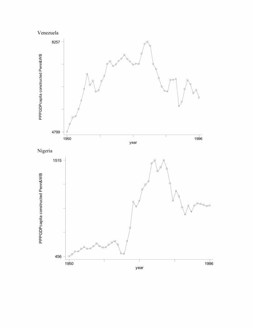
Figure 2

YN

YT

CTB

YTA

YTB

YNBYNA

THE BENCHMARK MODEL: THE DIVERSIFIED ECONOMY

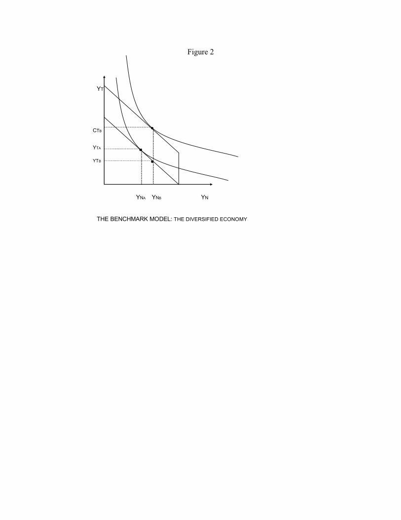
Figure 3

YT

CTB

= YNBYNA

CTA

=THE BENCHMARK MODEL: THE SPECIALIZEDIED ECONOMY

YT

CTB

= YNBYNA

CTA

=THE BENCHMARK MODEL: THE SPECIALIZEDIED ECONOMY

Figure 4.

Ψ

1−(1−α)β

NT

g(Ψ^α)

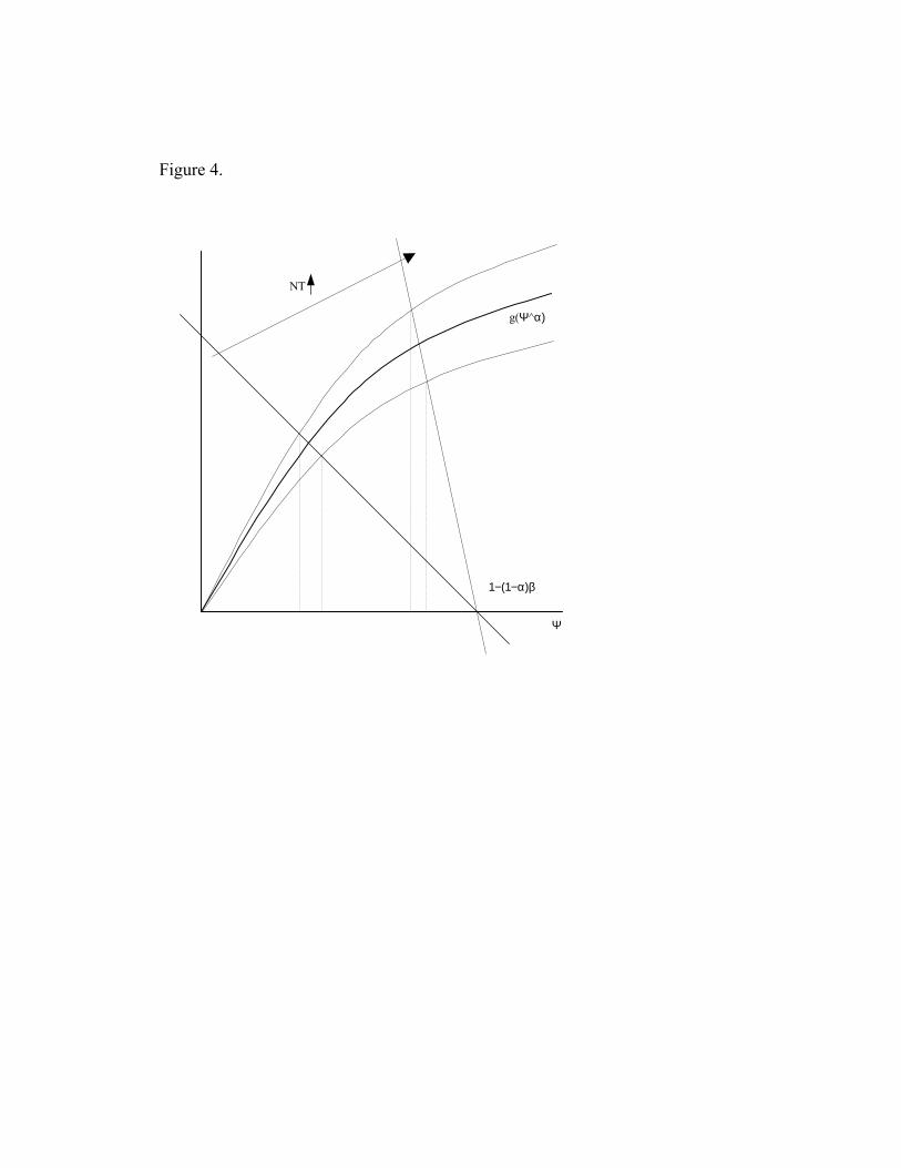
Figure 5. Simulation: the risk neutral case 5.a Number of non-tradable firms

3

4

5

6

7

8

9

0.1 0.2 0.3 0.4 0.5 0.6 0.7 0.8 0.9 1

0 0.25 0.75 0.875

5.b Number of tradable firms

0

0.5

1

1.5

2

2.5

3

3.5

4

4.5

5

0.1 0.2 0.3 0.4 0.5 0.6 0.7 0 .8 0.9 1

0 0.25 0.75 0.875

5.c Household utility

.d Real exchange rate volatility

0.8

0.85

0.9

0.95

1

1.05

0.1 0.2 0.3 0.4 0.5 0.6 0.7 0.8 0.9 1

0 0.25 0.75 0.875

5

0

0 .0 005

0 .001

0 .0 015

0 .002

0 .0 025

0 .1 0 .2 0 .3 0 .4 0 .5 0 .6 0 .7 0 .8 0 .9 1

0 0 .25 0 .75 0 .8 75

0 .003

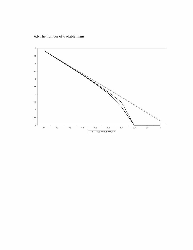
Figure 6. Silmulation: the risk-averse case 6.a The number of non-tradable firms

3

4

5

6

7

8

9

0.1 0.2 0.3 0.4 0.5 0.6 0.7 0.8 0.9 1

0 0.25 0.75 0.875

6.b The number of tradable firms

0

0.5

1

1.5

2

2.5

3

3.5

4

4.5

5

0.1 0.2 0.3 0.4 0.5 0.6 0.7 0.8 0.9 1

0 0.25 0.75 0.875

6.c Household utility

0.8

0.85

0.9

0.95

1

1.05

0.1 0.2 0.3 0.4 0.5 0.6 0.7 0.8 0.9 1

0 0.25 0.75 0.875

6.d Real exchange rate volatility

0

0.005

0.01

0.015

0.02

0.025

0.03

0.035

0.04

0.045

0.1 0.2 0.3 0.4 0.5 0.6 0.7 0.8 0.9 1

0 0.25 0.75 0.875