nber working paper series cross-country trends in
TRANSCRIPT

NBER WORKING PAPER SERIES
CROSS-COUNTRY TRENDS IN AFFECTIVE POLARIZATION
Levi BoxellMatthew Gentzkow
Jesse M. Shapiro
Working Paper 26669http://www.nber.org/papers/w26669
NATIONAL BUREAU OF ECONOMIC RESEARCH1050 Massachusetts Avenue
Cambridge, MA 02138January 2020, Revised November 2021
We thank James Adams, Klaus Desmet, John Duca, Ray Fair, Morris Fiorina, Greg Huber, Shanto Iyengar, Emir Kamenica, Rishi Kishore, Yphtach Lelkes, Matthew Levendusky, Neil Malhotra, Greg Martin, Eoin McGuirk, Pippa Norris, Carlo Schwarz, Sean Westwood, and seminar participants at the DC Political Economy Center Webinar, Stanford University, the Brown Data Science Initiative, the CREST Reading Group on Political Economy, and the American Economic Association for their comments and suggestions. We thank Lenka Drazanova and Philipp Rehm for sharing data, Dina Smeltz for sharing survey questionnaires, Rune Stubager for providing questionnaire translations, Will Horne for assistance with the CSES data, and Marc Swyngedouw for answering inquiries about the Belgium National Election Study. We also thank our many dedicated research assistants for their contributions to this project. We acknowledge funding from the Population Studies and Training Center, the Eastman Professorship, and the JP Morgan Chase Research Assistant Program at Brown University, the Stanford Institute for Economic Policy Research (SIEPR), the Institute for Humane Studies, the John S. and James L. Knight Foundation, and the Toulouse Network for Information Technology.This material is based upon work supported by the National Science Foundation Graduate Research Fellowship Program under Grant No. DGE-1656518. The research was also sponsored by the Army Research Office under Grant Number W911NF-20-1-0252. The U.S. Government is authorized to reproduce and distribute reprints for Government purposes notwithstanding any copyright notation herein. Any opinions, views, findings, and conclusions or recommendations expressed in this material are those of the authors and do not necessarily reflect the views or official policies of the National Science Foundation, the Army Research Office, the U.S. Government, National Bureau of Economic Research, the other funding sources, or the data sources. The appendix includes complete references for the data sources and therefore the references in the appendix should be considered as part of the references for this article.At least one co-author has disclosed additional relationships of potential relevance for this research. Further information is available online at http://www.nber.org/papers/w26669.ack
NBER working papers are circulated for discussion and comment purposes. They have not been peer-reviewed or been subject to the review by the NBER Board of Directors that accompanies official NBER publications.
© 2020 by Levi Boxell, Matthew Gentzkow, and Jesse M. Shapiro. All rights reserved. Short sections of text, not to exceed two paragraphs, may be quoted without explicit permission provided that full credit, including © notice, is given to the source.

Cross-Country Trends in Affective PolarizationLevi Boxell, Matthew Gentzkow, and Jesse M. Shapiro NBER Working Paper No. 26669January 2020, Revised November 2021JEL No. D72
ABSTRACT
We measure trends in affective polarization in twelve OECD countries over the past four decades.According to our baseline estimates, the US experienced the largest increase in polarization over thisperiod. Five countries experienced a smaller increase in polarization. Six countries experienced a decreasein polarization. We relate trends in polarization to trends in potential explanatory factors.
Levi BoxellStanford University, Department of Economics579 Jane Stanford WayStanford, CA [email protected]
Matthew GentzkowDepartment of EconomicsStanford University579 Jane Stanford WayStanford, CA 94305and [email protected]
Jesse M. ShapiroEconomics DepartmentBox BBrown UniversityProvidence, RI 02912and [email protected]

1 Introduction
Affective polarization refers to the extent to which citizens feel more negatively toward other po-
litical parties than toward their own (Iyengar et al. 2019). Affective polarization has risen substan-
tially in the US in recent decades (Iyengar et al. 2019). In 1978, according to our calculations, the
average partisan rated in-party members 27.4 points higher than out-party members on a “feeling
thermometer” ranging from 0 to 100. In 2020 the difference was 56.3, implying an increase of
1.08 standard deviations as measured in the 1978 distribution. Growing affective polarization may
have important consequences, including reducing the efficacy of government (Hetherington and
Rudolph 2015),1 increasing the homophily of social groups (Iyengar et al. 2012; Iyengar et al.
2019), and altering economic decisions (Gift and Gift 2015; Iyengar et al. 2019).
Partly due to the difficulty of constructing harmonized data series on partisan affect, there is
limited evidence on long-term trends in affective polarization in developed democracies other than
the US. Cross-country comparisons can help assess why affective polarization has risen in the
US. If affective polarization has risen in countries other than the US, then examining commonal-
ities may suggest promising explanations for the US experience. If affective polarization has not
risen elsewhere, then it may be fruitful to examine factors that help distinguish the US from other
developed democracies.
In this paper, we present the first cross-country evidence on trends in affective polarization
since the 1980s, focusing on twelve OECD countries. In our baseline analysis, we find that the
US exhibited the largest increase in affective polarization over this period. In five other coun-
tries—Switzerland, France, Denmark, Canada, and New Zealand—polarization also rose, but to
a lesser extent. In six other countries—Japan, Australia, Britain, Norway, Sweden, and (West)
Germany—polarization fell.
1See also Kimball et al. (2018). Commentators expressing related concerns include Obama (2010), Blankenhorn
(2015), and Drutman (2017). A 2018 survey shows that more than 70 percent of foreign policy opinion leaders con-
sider political polarization a “critical threat” facing the US, ranking it above issues such as foreign nuclear programs
(Smeltz et al. 2018).
2
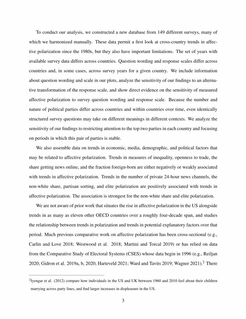
To conduct our analysis, we constructed a new database from 149 different surveys, many of
which we harmonized manually. These data permit a first look at cross-country trends in affec-
tive polarization since the 1980s, but they also have important limitations. The set of years with
available survey data differs across countries. Question wording and response scales differ across
countries and, in some cases, across survey years for a given country. We include information
about question wording and scale in our plots, analyze the sensitivity of our findings to an alterna-
tive transformation of the response scale, and show direct evidence on the sensitivity of measured
affective polarization to survey question wording and response scale. Because the number and
nature of political parties differ across countries and within countries over time, even identically
structured survey questions may take on different meanings in different contexts. We analyze the
sensitivity of our findings to restricting attention to the top two parties in each country and focusing
on periods in which this pair of parties is stable.
We also assemble data on trends in economic, media, demographic, and political factors that
may be related to affective polarization. Trends in measures of inequality, openness to trade, the
share getting news online, and the fraction foreign-born are either negatively or weakly associated
with trends in affective polarization. Trends in the number of private 24-hour news channels, the
non-white share, partisan sorting, and elite polarization are positively associated with trends in
affective polarization. The association is strongest for the non-white share and elite polarization.
We are not aware of prior work that situates the rise in affective polarization in the US alongside
trends in as many as eleven other OECD countries over a roughly four-decade span, and studies
the relationship between trends in polarization and trends in potential explanatory factors over that
period. Much previous comparative work on affective polarization has been cross-sectional (e.g.,
Carlin and Love 2018; Westwood et al. 2018; Martini and Torcal 2019) or has relied on data
from the Comparative Study of Electoral Systems (CSES) whose data begin in 1996 (e.g., Reiljan
2020; Gidron et al. 2019a, b, 2020; Harteveld 2021; Ward and Tavits 2019; Wagner 2021).2 There
2Iyengar et al. (2012) compare how individuals in the US and UK between 1960 and 2010 feel about their children
marrying across party lines, and find larger increases in displeasure in the US.
3

is also previous comparative work studying dimensions of mass polarization, such as ideological
polarization, that may have causes and consequences distinct from those of affective polarization
(Iyengar et al. 2019). For example, Draca and Schwarz (2021) analyze data from the World and
European Values Surveys from 1989 through 2010 and find that the US experienced the largest
increase in ideological polarization among the 17 countries considered.3
The remainder of the paper is organized as follows. Section 2 describes our data sources and
measure of affective polarization. Section 3 presents our findings on trends in affective polariza-
tion. Section 4 presents our findings on the relationship between trends in affective polarization
and trends in potential explanatory factors. Section 5 concludes.
2 Data and Measure of Affective Polarization
Among members of the OECD as of 1973, there are ten, including the US, for which we are aware
of an election study with a partisan affect question prior to 1985. Our sample includes these ten
countries, as well as Australia and New Zealand, which we believe make interesting comparisons
to the US. Appendix Figure 10 and Appendix Table 2 provide information on data availability for
all 1973 OECD members, including those we do not include in our sample. We extract a survey
weight associated with each respondent. Appendices A.5 and A.6 detail the survey variables and
data sources for each sample country and included survey year.
We extract each respondent’s party identification, excluding “leaners” who only choose a party
identification in response to a second prompt. We exclude “leaners” from our sample because not
all surveys include a second prompt.4 Appendix Figure 1 depicts trends in the share of respondents
identifying with a party and the share of affiliates who are affiliated with the top two parties,
3Some other studies examine long-term trends in mass polarization in individual countries outside the United States,
including Canada (Kevins and Soroka 2018), Germany (Munzert and Bauer 2013), Britain (Adams et al. 2012a, b),
and the Netherlands (Adams et al. 2011), but do not report trends in affective polarization.
4Keith et al. (1992) discuss the interpretation of “leaners.”
4

separately by country.
We extract a measure of each respondent’s affect toward the parties in the respondent’s country.
Questions about affect vary across surveys, commonly asking respondents how they feel toward
a given party, how much they like the party, or to what extent they sympathize with the party.5
Numerical response scales also differ across surveys. We apply an affine transformation to the
responses in each survey so that the minimum transformed response is 0 and the maximum trans-
formed response is 100. We refer to the transformed response as the respondent’s reported affect
toward the given party.
To define affective polarization, fix a given survey and let P denote the set of parties toward
which respondents are asked their affect. Let N denote the set of respondents with non-zero
weight who both provide a valid party identification in P and report a valid affect toward their
own party and at least one other party in P .6 For each respondent i ∈N , let p(i) ∈P denote the
party with which the respondent identifies and let Pi ⊆P denote the set of parties toward which
the respondent reports a valid affect. Let Api ∈ [0,100] denote the reported affect of respondent
i toward party p ∈Pi. Finally, let wi ≥ 0 denote the survey weight of respondent i ∈ N and
let W (P ′) = ∑{i∈N :p(i)∈P ′}wi denote the weighted number of respondents in any set of parties
P ′ ⊆P , with W (P) denoting the weighted number of respondents in N .
We define the partisan affect πi of respondent i as
πi = ∑p′∈Pi\p(i)
W (p′)W (Pi)−W (p(i))
(Ap(i)
i −Ap′i
).
Partisan affect πi reflects the extent to which respondent i expresses a more favorable attitude
toward her own party than toward other parties.
5Druckman and Levendusky (2019) study the interpretation of such questions.
6We iteratively define P and N after excluding parties with zero affiliates in N from P .
5

We define affective polarization Π as the weighted average of respondents’ partisan affect:
Π = ∑i∈N
wi
W (P)πi.
If there are two parties and all respondents state their affect toward both, then affective polarization
Π is the difference between weighted mean own-party affect and weighted mean other-party affect,
as in Iyengar et al. (2019).7 In the multi-party case, our definition is similar to ones adopted by
Gidron et al. (2019b, 2020, equations 1 and 2), Reiljan (2020, equation 3), and Harteveld (2021,
equation 1).8
We obtain data on various potential explanatory variables at the level of the country and year
from a range of sources that are detailed in Appendix A.7. We try to collect variables that can be
measured reasonably well across different countries and years, and that have been linked in the
literature to the rise in affective polarization. Though not exhaustive, we believe that the variables
we collect reflect many of the important factors that meet these criteria.
3 Comparison of Trends in Affective Polarization
Figure 1 shows the time path of affective polarization in each of the twelve countries that we study.
Plot markers indicate the response scaling in the original survey question. The depicted intervals
constitute a uniform 95 percent confidence band for affective polarization, computed following
Montiel Olea and Plagborg-Møller (2019).
Each plot depicts an estimated linear time trend and reports its slope. For no country does the
7In this case:
Π = ∑i∈N
wi
W (P)Ap(i)
i − ∑i∈N
wi
W (P)AP\p(i)
i .
8See also Wagner (2021, section 4.1).
6

uniform confidence band contain the linear fit, indicating that the linear fit should be taken only as
a convenient summary of the average change, not as a complete description of the dynamics of the
series.9 Each plot also reports the 95 percent confidence interval for the slope of the linear trend,
computed following Imbens and Kolesar (2016). Although these intervals and associated p−values
are designed for small-sample settings (using an adjustment from Bell and McCaffrey 2002), we
nevertheless suggest interpreting statements of statistical significance regarding the linear trends
with caution, especially for countries with relatively few survey years.
Consistent with the existing evidence (e.g., Iyengar et al. 2019), Figure 1 shows that affective
polarization grew rapidly in the US over the sample period. The estimated linear trend is 5.6 points
per decade (p−value < 0.001). For comparison, the standard deviation in partisan affect in the base
period of 1978 was 26.7.
Five other countries—Switzerland, France, Denmark, Canada, and New Zealand—exhibit a
smaller positive trend. The trend is statistically significant for Denmark. Switzerland’s is the
largest trend of the five, with a slope of 5.1 points per decade (p−value = 0.090). Panel A of Table
1 shows that we can reject the (pairwise) equality of linear trends between the US and each of the
five other countries with a positive trend, except Switzerland.
The remaining six countries—Japan, Australia, Britain, Norway, Sweden, and Germany—exhibit
a negative linear trend, which is statistically significant for Sweden and Germany. Germany ex-
hibits the largest negative trend, equal to 3.7 points per decade (p−value < 0.001), which can be
compared to a standard deviation in partisan affect in the base period of 1977 of 25.4. Panel A of
Table 1 shows that we can reject the (pairwise) equality of trends between the US and each of the
six countries with a negative linear trend.
Appendix Figure 2 breaks down the trends in affective polarization into affect toward the re-
spondent’s own party and affect toward other parties. Consistent with an existing literature on
9Some countries appear to exhibit cyclicality in affective polarization. In some of these countries (e.g., Britain),
the surveys we rely on coincide with elections, suggesting that election years themselves are not the source of the
apparent cyclicality.
7
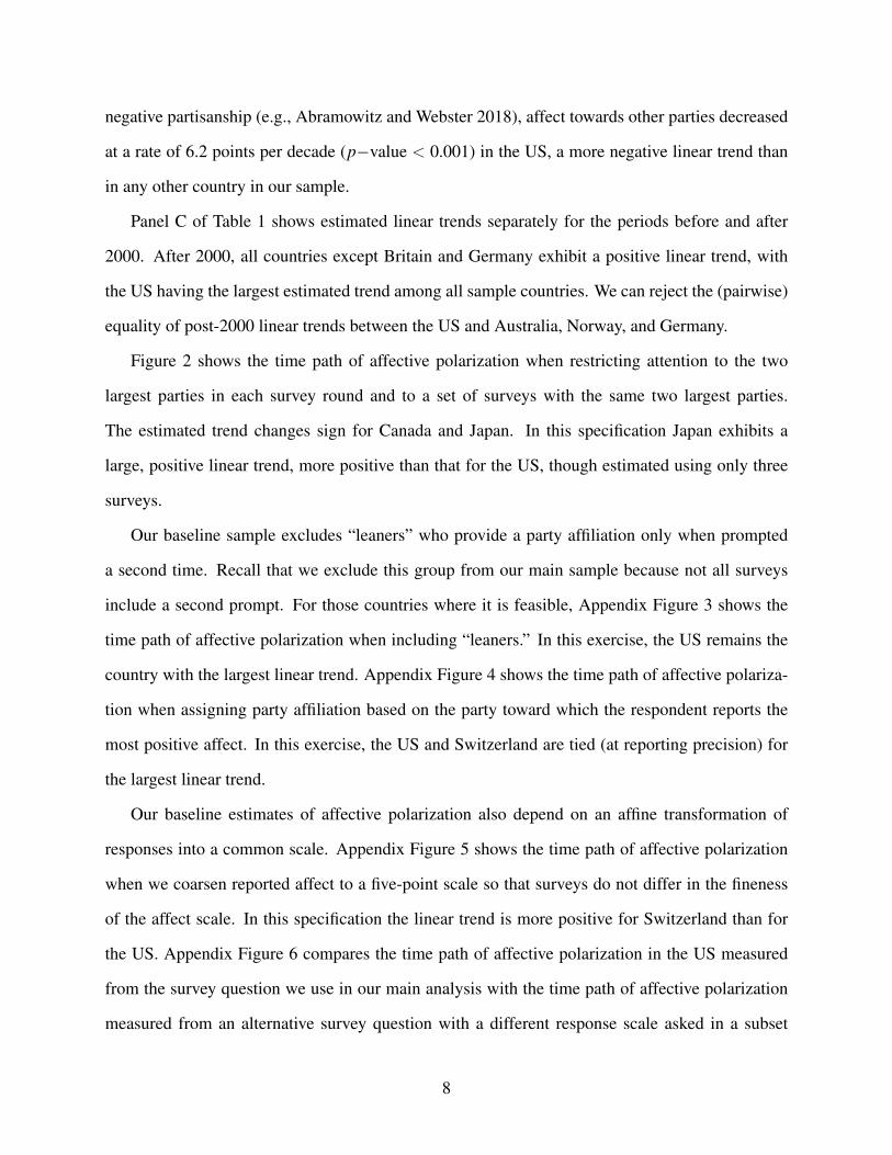
negative partisanship (e.g., Abramowitz and Webster 2018), affect towards other parties decreased
at a rate of 6.2 points per decade (p−value < 0.001) in the US, a more negative linear trend than
in any other country in our sample.
Panel C of Table 1 shows estimated linear trends separately for the periods before and after
2000. After 2000, all countries except Britain and Germany exhibit a positive linear trend, with
the US having the largest estimated trend among all sample countries. We can reject the (pairwise)
equality of post-2000 linear trends between the US and Australia, Norway, and Germany.
Figure 2 shows the time path of affective polarization when restricting attention to the two
largest parties in each survey round and to a set of surveys with the same two largest parties.
The estimated trend changes sign for Canada and Japan. In this specification Japan exhibits a
large, positive linear trend, more positive than that for the US, though estimated using only three
surveys.
Our baseline sample excludes “leaners” who provide a party affiliation only when prompted
a second time. Recall that we exclude this group from our main sample because not all surveys
include a second prompt. For those countries where it is feasible, Appendix Figure 3 shows the
time path of affective polarization when including “leaners.” In this exercise, the US remains the
country with the largest linear trend. Appendix Figure 4 shows the time path of affective polariza-
tion when assigning party affiliation based on the party toward which the respondent reports the
most positive affect. In this exercise, the US and Switzerland are tied (at reporting precision) for
the largest linear trend.
Our baseline estimates of affective polarization also depend on an affine transformation of
responses into a common scale. Appendix Figure 5 shows the time path of affective polarization
when we coarsen reported affect to a five-point scale so that surveys do not differ in the fineness
of the affect scale. In this specification the linear trend is more positive for Switzerland than for
the US. Appendix Figure 6 compares the time path of affective polarization in the US measured
from the survey question we use in our main analysis with the time path of affective polarization
measured from an alternative survey question with a different response scale asked in a subset
8

of survey years. The estimated trends differ by 1.2 points per decade (SE = 0.7), which can be
compared to a baseline trend of 6.4 points per decade. Appendix Figure 7 compares measured
affective polarization between our data sources and those in the CSES.
Panel B of Table 1 reports the estimated trends and confidence intervals for the sensitivity
analyses in Appendix Figures 3–5.
4 Comparison of Trends in Potential Explanatory Factors
Figure 3 presents evidence on trends in potential explanatory factors. Each panel corresponds to a
different group of variables. Each plot within a panel corresponds to a different variable. Each plot
is a scatterplot where the y-axis is the estimated linear trend in affective polarization, the x-axis
is the estimated linear trend in the explanatory variable, and an observation is a country. Each
plot also reports the Spearman rank correlation between the two trends and the p−value from a
permutation test of the statistical significance of the rank correlation. The line of best fit is also
plotted. Appendix Figure 8 plots the individual series for each of the explanatory variables that we
consider.
With only twelve countries in our sample, it is difficult to draw firm conclusions about the
association between trends in affective polarization and trends in explanatory factors, especially
because trends in explanatory variables are correlated across countries. Moreover, our analysis
necessarily includes only a subset of the potentially important factors. Appendix Table 1 reports
the pairwise Spearman rank correlation across the linear trends in the explanatory variables used
in Figure 3, and Appendix Figure 9 presents scatterplots for additional potential explanatory vari-
ables.
Panel A of Figure 3 considers economic and media-related variables. A number of authors
(e.g., Payne 2017; Pearlstein 2018) have linked polarization in the US to growing inequality and
other related economic changes. Similarly, a number of authors (e.g., Lelkes et al. 2017; Sunstein
2017; Settle 2018) have linked polarization in the US to the rise of digital media, and others (e.g.,
9

Duca and Saving 2017; Martin and Yurukoglu 2017) have linked the growth in polarization to the
rise of partisan cable news networks in the US.10 None of the plots in Panel A of Figure 3 exhibits
a statistically significant rank correlation between the linear trend in the explanatory variable and
the linear trend in affective polarization.
Panel B of Figure 3 considers demographic and political variables. Many authors (e.g., Mason
2016, 2018; Valentino and Zhirkov 2018; Abramowitz 2018; Mason and Wronski 2018; Westwood
and Peterson 2020) have suggested connections between affective polarization and racial and other
social divisions.11 The linear trend in the share foreign born has a negative and statistically in-
significant rank correlation with the linear trend in affective polarization. The linear trend in the
non-white share of the population has a positive rank correlation with the linear trend in affective
polarization, with an associated p−value of 0.052.
There is also evidence of growing partisan-ideological sorting in the US in recent decades (e.g.,
Fiorina and Abrams 2008; Levendusky 2009; Fiorina 2016, 2017), and this may have influenced
the growth in affective polarization (e.g., Webster and Abramowitz 2017; Lelkes 2018; Orr and
Huber 2020).12 The linear trend in partisan-ideological sorting has a positive and statistically
insignificant rank correlation with the linear trend in affective polarization.
Elite polarization increased in the US over the period we study (e.g., McCarty et al. 2006)
and changes in elite polarization may influence affective polarization (e.g., Banda and Cluverius
2018).13 The linear trend in elite polarization has a positive and statistically significant rank corre-
10But see also, e.g., Arceneaux and Johnson (2013).
11See also Craig et al. (2018), Bertrand and Kamenica (2018), and Desmet and Wacziarg (2021).
12See Fiorina (2017, chapter 8) for a discussion of cross-country differences in sorting, and see Kevins and Soroka
(2018) and Adams et al. (2012a) for studies on partisan sorting in Canada and Britain respectively.
13See also Rehm and Reilly (2010). Elite polarization may of course be influenced by affective polarization as well as
the reverse. Within the US, some aspects of the growth in elite polarization, such as the realignment of the parties
in the South following the civil rights era, seem to originate at least in part in the strategic choices of political elites
rather than the shifting views of voters themselves (Fiorina and Abrams 2008, p. 581; Levendusky 2009, 2010; Lupu
2015; Banda and Cluverius 2018). Regarding the Southern realignment, see Black and Black (2002), Valentino and
10

lation with the linear trend in affective polarization (p−value = 0.011)
5 Conclusion
The main contribution of our paper is to situate the rapid rise in affective polarization in the US
over the preceding four decades in an international context. According to our baseline estimates,
the US experienced the most rapid growth in affective polarization over this period among the
twelve OECD countries we consider, with five other countries experiencing smaller increases in
polarization, and six experiencing declines in polarization.
A secondary contribution of our paper is to examine the relationship between trends in affective
polarization and trends in a set of potential explanatory variables. In some cases (e.g., the non-
white share of the population and elite polarization), there is evidence of a positive association
between the trend in the explanatory variable and the trend in affective polarization; in other cases
(e.g., inequality, the trade share of GDP, and internet penetration), there is not.
Our analysis has important limitations. Differences in survey format, political systems, and
other factors make cross-country comparisons of affective polarization challenging. Well-known
limitations of cross-country data (e.g., Mankiw 1995) make it difficult to reach firm conclusions
about the causal role of different explanatory factors. Furthermore, though we have attempted to
measure variables that capture many of the most prominent explanations for the rise in affective
polarization in the US, we have not measured all of them. For example, an existing literature relates
mass polarization to the extent to which a person’s political party is aligned with other aspects of
the person’s identity, such as their race or religion (Mason, 2016, 2018; Mason and Wronski 2018).
Measuring this type of social sorting in a comparable way across countries, and relating trends in
social sorting to the long-term trends in affective polarization that we have documented here, seems
an interesting direction for future work.14
Sears (2005), and Kuziemko and Washington (2018).
14Harteveld (2021) studies the relationship between affective polarization and measures of social sorting in a panel of
11

References
Abramowitz, Alan I. 2018. The Great Alignment: Race, Party Transformation, and the Rise of
Donald Trump. New Haven, CT: Yale University Press.
Abramowitz, Alan I., and Steven W. Webster. 2018. “Negative Partisanship: Why Americans
Dislike Parties but Behave Like Rabid Partisans.” Advances in Political Psychology 39 (S1):
119–135.
Adams, James, Catherine E. De Vries, and Debra Leiter. 2011. “Subconstituency Reactions to
Elite Depolarization in the Netherlands: An Analysis of the Dutch Public’s Policy Beliefs and
Partisan Loyalties, 1986–98.” British Journal of Political Science 42 (1): 81–105.
Adams, James, Jane Green, and Caitlin Milazzo. 2012a. “Has the British Public Depolarized
Along With Political Elites? An American Perspective on British Public Opinion.” Compar-
ative Political Studies 45 (4): 507–530.
Adams, James, Jane Green, and Caitlin Milazzo. 2012b. “Who Moves? Elite and Mass-Level
Depolarization in Britain, 1987–2001.” Electoral Studies 31 (4): 643–655.
Arceneaux, Kevin, and Martin Johnson. 2013. Changing Minds or Changing Channels?: Partisan
News in an Age of Choice. Chicago, IL: University of Chicago Press.
Banda, Kevin K., and John Cluverius. 2018. “Elite Polarization, Party Extremity, and Affective
Polarization.” Electoral Studies 56: 90–101.
Bell, Robert M. and Daniel F. McCaffrey. 2002. “Bias Reduction in Standard Errors for Linear
Regression with Multi-Stage Samples.” Survey Methodology 28 (2): 169-181.
Bertrand, Marianne, and Emir Kamenica. 2018. “Coming Apart? Cultural Distances in the United
States over Time.” NBER Working Paper 24771. Accessed at http://www.nber.org/papers/w24771
on July 21, 2021.
Best, D. J., and D. E. Roberts. 1975. “Algorithm AS 89: The Upper Tail Probabilities of Spear-
man’s Rho.” Journal of the Royal Statistical Society, Series C (Applied Statistics) 24 (3):
377–379.
countries drawn from the CSES.
12

Black, Earl, and Merle Black. 2002. The Rise of Southern Republicans. Cambridge, MA: Harvard
University Press.
Blankenhorn, David. 2015. “Why Polarization Matters.” The American Interest, December 22,
2015. Accessed at https://www.the-american-interest.com/2015/12/22/why-polarization-matters/
on September 23, 2019.
Carlin, Ryan E., and Gregory J. Love. 2018. “Political Competition, Partisanship and Interpersonal
Trust in Electoral Democracies.” British Journal of Political Science 48 (1): 115–139.
Craig, Maureen A., Julian M. Rucker, and Jennifer A. Richeson. 2018. “Racial and Political Dy-
namics of an Approaching ‘Majority-Minority’ United States.” The ANNALS of the American
Academy of Political and Social Science 677 (1): 204–214.
Desmet, Klaus, and Romain Wacziarg. 2021. “The Cultural Divide.” The Economic Journal 131
(637): 2058–2088.
Draca, Mirko, and Carlo Schwarz. 2021. “How Polarized are Citizens? Measuring Ideology from
the Ground-Up.” Working Paper. Accessed at
https://papers.ssrn.com/sol3/papers.cfm?abstract id=3154431 on May 30, 2021.
Druckman, James N., and Matthew S. Levendusky. 2019. “What do We Measure When We
Measure Affective Polarization?” Public Opinion Quarterly 83 (1): 114–122.
Drutman, Lee. 2017. “We Need Political Parties. But Their Rabid Partisanship Could Destroy
American Democracy.” Vox, September 5, 2017. Accessed at https://www.vox.com/the-big-
idea/2017/9/5/16227700/ hyperpartisanship-identity-american-democracy-problems-solutions-
doom-loop on September 23, 2019.
Duca, John V., and Jason L. Saving. 2017. “Income Inequality, Media Fragmentation, and In-
creased Political Polarization.” Contemporary Economic Policy 35 (2): 392–413.
Fiorina, Morris P., and Samuel J. Abrams. 2008. “Political Polarization in the American Public.”
Annual Review of Political Science 11: 563–588.
Fiorina, Morris P. 2016. “The Political Parties Have Sorted.” Hoover Institution Essay on Contem-
porary American Politics (3).
13

Fiorina, Morris P. 2017. Unstable Majorities: Polarization, Party Sorting and Political Stalemate.
Stanford, CA: Hoover Institution Press.
Gidron, Noam, James Adams, and Will Horne. 2019a. “Toward a Comparative Research Agenda
on Affective Polarization in Mass Publics.” APSA Comparative Politics Newsletter 29 (1):
30–36.
Gidron, Noam, James Adams, and Will Horne. 2019b. “How Ideology, Economics and Insti-
tutions Shape Affective Polarization in Democratic Polities.” Working Paper. Accessed at
https://ces.fas.harvard.edu/uploads/files/events/
GAH-Affective-Polarization-in-Democratic-Polities.pdf on May 30, 2021.
Gidron, Noam, James Adams, and Will Horne. 2020. American Affective Polarization in Compar-
ative Perspective. Cambridge, UK: Cambridge University Press.
Gift, Karen, and Thomas Gift. 2015. “Does Politics Influence Hiring? Evidence from a Random-
ized Experiment.” Political Behavior 37 (3): 653–675.
Harteveld, Eelco. 2021. “Ticking All the Boxes? A Comparative Study of Social Sorting and
Affective Polarization.” Electoral Studies 72: 102337.
Hetherington, Marc J., and Thomas J. Rudolph. 2015. Why Washington Won’t Work: Polarization,
Trust, and the Governing Crisis. Chicago, IL: University of Chicago Press.
Imbens, Guido W., and Michal Kolesar. 2016. “Robust Standard Errors in Small Samples: Some
Practical Advice.” Review of Economics and Statistics 98 (4): 701–712.
Iyengar, Shanto, Gaurav Sood, and Yphtach Lelkes. 2012. “Affect, Not Ideology: A Social Identity
Perspective on Polarization.” Public Opinion Quarterly 76 (3): 405–431.
Iyengar, Shanto, Yphtach Lelkes, Matthew Levendusky, Neil Malhotra, and Sean J. Westwood.
2019. “The Origins and Consequences of Affective Polarization in the United States.” Annual
Review of Political Science 22: 129–146.
Keith, Bruce E., David B. Magleby, Candice J. Nelson, Elizabeth A. Orr, Mark C. Westlye, and
Raymond E. Wolfinger. 1992. The Myth of the Independent Voter. Berkeley, CA: University
of California Press.
14

Kevins, Anthony, and Stuart N. Soroka. 2018. “Growing Apart? Partisan Sorting in Canada,
1992–2015.” Canadian Journal of Political Science 51 (1): 103–133.
Kimball, David C., Joseph Anthony, and Tyler Chance. 2018. “Political Identity and Party Po-
larization in the American Electorate.” In The State of Parties 2018: The Changing Role of
Contemporary American Political Parties, edited by John C. Green, Daniel J. Coffey, and
David B. Cohen, 169-184. Lanham, MD: Rowman and Littlefield.
Kuziemko, Ilyana, and Ebonya Washington. 2018. “Why Did the Democrats Lose the South?
Bringing New Data to an Old Debate.” American Economic Review 108 (10): 2830–2867.
Lelkes, Yphtach. 2018. “Affective Polarization and Ideological Sorting: A Reciprocal, Albeit
Weak, Relationship.” The Forum 16 (1): 67–79.
Lelkes, Yphtach, Gaurav Sood, and Shanto Iyengar. 2017. “The Hostile Audience: The Effect of
Access to Broadband Internet on Partisan Affect.” American Journal of Political Science 61
(1): 5–20.
Levendusky, Matthew. 2009. The Partisan Sort: How Liberals became Democrats and Conserva-
tives became Republicans. Chicago, IL: University of Chicago Press.
Levendusky, Matthew S. 2010. “Clearer Cues, More Consistent Voters: A Benefit of Elite Polar-
ization.” Political Behavior 32 (1): 111–131.
Lupu, Noam. 2015. “Party Polarization and Mass Partisanship: A Comparative Perspective.”
Political Behavior 37 (2): 331–356.
Mankiw, N. Gregory. 1995. “The Growth of Nations.” Brookings Papers on Economic Activity
1995 (1): 275–326.
Martin, Gregory J., and Ali Yurukoglu. 2017. “Bias in Cable News: Persuasion and Polarization.”
American Economic Review 107 (9): 2565–2599.
Martini, Sergio, and Mariano Torcal. 2019. “Trust Across Political Conflicts: Evidence from a
Survey Experiment in Divided Societies.” Party Politics 25 (2): 126–139.
Mason, Lilliana. 2016. “A Cross-Cutting Calm: How Social Sorting Drives Affective Polariza-
tion.” Public Opinion Quarterly 80 (S1): 351–377.
15

Mason, Lilliana. 2018. Uncivil Agreement: How Politics Became Our Identity. Chicago, IL:
University of Chicago Press.
Mason, Lilliana, and Julie Wronski. 2018. “One Tribe to Bind Them All: How Our Social Group
Attachments Strengthen Partisanship.” Advances in Political Psychology 39 (S1): 257–277.
McCarty, Nolan, Keith T. Poole, and Howard Rosenthal. 2006. Polarized America: The Dance of
Ideology and Unequal Riches. Cambridge, MA: MIT Press.
Montiel Olea, Jose Luis, and Mikkel Plagborg-Møller. 2019. “Simultaneous Confidence Bands:
Theory, Implementation, and an Application to SVARs.” Journal of Applied Econometrics 34
(1): 1–17.
Munzert, Simon, and Paul C. Bauer. 2013. “Political Depolarization in German Public Opinion,
1980–2010.” Political Science Research and Methods 1 (1): 67–89.
Obama, Barack. 2010. “Remarks by the President at University of Michigan Spring Commence-
ment.” Speech, Ann Arbor, MI, May 1, 2010. The White House. Accessed at
https://obamawhitehouse.archives.gov/the-press-office/remarks-president-university-michigan-
spring-commencement on September 23, 2019.
Orr, Lilla V., and Gregory A. Huber. 2020. “The Policy Basis of Measured Partisan Animosity in
the United States.” American Journal of Political Science 64 (3): 569-586.
Payne, Keith. 2017. The Broken Ladder: How Inequality Affects the Way We Think, Live, and Die.
New York, NY: Penguin Books.
Pearlstein, Steven. 2018. Can American Capitalism Survive?: Why Greed Is Not Good, Opportu-
nity is Not Equal, and Fairness Won’t Make Us Poor. New York, NY: St. Martin’s Press.
Rehm, Philipp, and Timothy Reilly. 2010. “United We Stand: Constituency Homogeneity and
Comparative Party Polarization.” Electoral Studies 29 (1): 40–53.
Reiljan, Andres. 2020. “‘Fear and Loathing Across Party Lines’ (also) in Europe: Affective Polar-
isation in European Party Systems.” European Journal of Political Research 59 (2): 376–396.
Settle, Jaime E. 2018. Frenemies: How Social Media Polarizes America. New York, NY: Cam-
bridge University Press.
16

Smeltz, Dina, Joshua Busby, and Jordan Tama. 2018. “Political Polarization the Critical Threat to
US, Foreign Policy Experts Say.” The Hill, November 9, 2018. Accessed at https://thehill.com/
opinion/national-security/415881-political-polarization-is-the-critical-threat-to-us-foreign-policy
on September 23, 2019.
Sunstein, Cass R. 2017. #Republic: Divided Democracy in the Age of Social Media. Princeton,
NJ: Princeton University Press.
Valentino, Nicholas A., and David O. Sears. 2005. “Old Times There Are Not Forgotten: Race
and Partisan Realignment in the Contemporary South.” American Journal of Political Science
49 (3): 672–688.
Valentino, Nicholas A., and Kirill Zhirkov. 2018. “Blue is Black and Red is White? Affective Po-
larization and the Racialized Schemas of U.S. Party Coalitions.” Working Paper. Accessed at
https://economics.sites.stanford.edu/sites/g/files/sbiybj9386/f/pe 04 17 valentino.pdf on May
30, 2021.
Wagner, Markus. 2021. “Affective Polarization in Multiparty Systems.” Electoral Studies 69:
102199.
Ward, Dalston G., and Margit Tavits. 2019. “How Partisan Affect Shapes Citizens’ Perception of
the Political World.” Electoral Studies 60: 102045.
Webster, Steven W., and Alan I. Abramowitz. 2017. “The Ideological Foundations of Affective
Polarization in the U.S. Electorate.” American Politics Research 45 (4): 621–647.
Westwood, Sean J., Shanto Iyengar, Stefaan Walgrave, Rafael Leonisio, Luis Miller, and Oliver
Strijbis. 2018. “The Tie that Divides: Cross-National Evidence of the Primary of Partyism.”
European Journal of Political Research 57 (2): 333–354.
Westwood, Sean J., and Erik Peterson. 2020. “The Inseparability of Race and Partisanship in the
United States.” Political Behavior. Forthcoming.
17
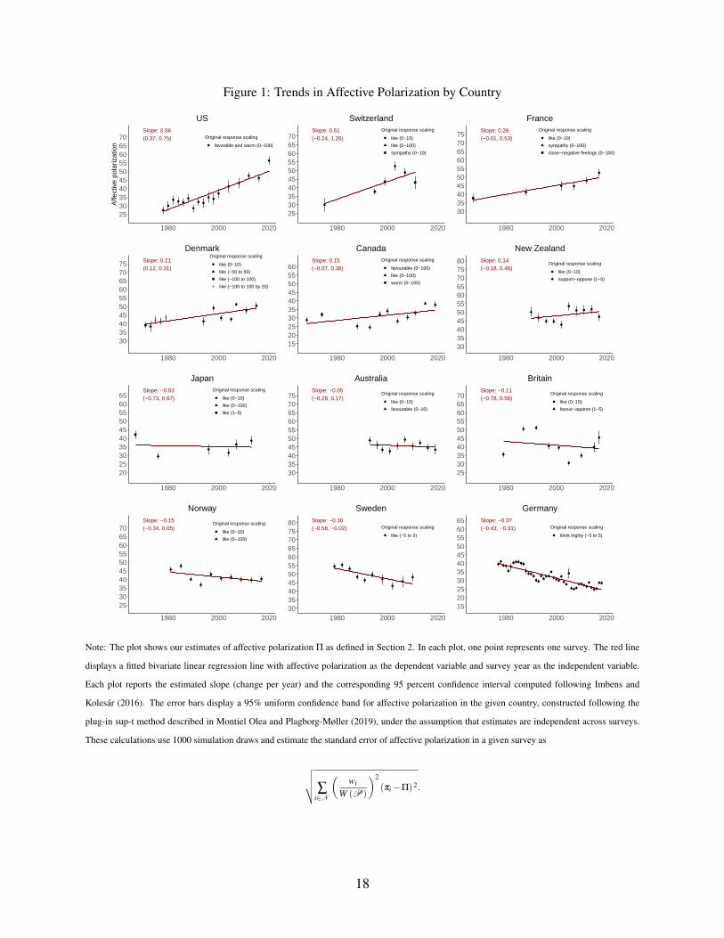
Figure 1: Trends in Affective Polarization by Country
Slope: 0.56(0.37, 0.75)
25303540455055606570
1980 2000 2020
Affe
ctiv
e po
lariz
atio
n
Original response scaling
favorable and warm (0−100)
USSlope: 0.51(−0.24, 1.26)
25303540455055606570
1980 2000 2020
Original response scaling
like (0−10)
like (0−100)
sympathy (0−10)
SwitzerlandSlope: 0.26(−0.01, 0.53)
30354045505560657075
1980 2000 2020
Original response scaling
like (0−10)
sympathy (0−100)
close−negative feelings (0−100)
France
Slope: 0.21(0.12, 0.31)
30354045505560657075
1980 2000 2020
Original response scaling
like (0−10)
like (−50 to 50)
like (−100 to 100)
like (−100 to 100 by 20)
DenmarkSlope: 0.15(−0.07, 0.38)
15202530354045505560
1980 2000 2020
Original response scaling
favourable (0−100)
like (0−100)
warm (0−100)
CanadaSlope: 0.14(−0.18, 0.46)
3035404550556065707580
1980 2000 2020
Original response scaling
like (0−10)
support−oppose (1−5)
New Zealand
Slope: −0.03(−0.73, 0.67)
20253035404550556065
1980 2000 2020
Original response scaling
like (0−10)
like (0−100)
like (1−5)
JapanSlope: −0.05(−0.28, 0.17)
30354045505560657075
1980 2000 2020
Original response scaling
like (0−10)
favourable (0−10)
AustraliaSlope: −0.11(−0.78, 0.56)
25303540455055606570
1980 2000 2020
Original response scaling
like (0−10)
favour−against (1−5)
Britain
Slope: −0.15(−0.34, 0.05)
25303540455055606570
1980 2000 2020
Original response scaling
like (0−10)
like (0−100)
NorwaySlope: −0.30(−0.58, −0.02)
3035404550556065707580
1980 2000 2020
Original response scaling
like (−5 to 5)
SwedenSlope: −0.37(−0.43, −0.31)
1520253035404550556065
1980 2000 2020
Original response scaling
think highly (−5 to 5)
Germany
Note: The plot shows our estimates of affective polarization Π as defined in Section 2. In each plot, one point represents one survey. The red line
displays a fitted bivariate linear regression line with affective polarization as the dependent variable and survey year as the independent variable.
Each plot reports the estimated slope (change per year) and the corresponding 95 percent confidence interval computed following Imbens and
Kolesar (2016). The error bars display a 95% uniform confidence band for affective polarization in the given country, constructed following the
plug-in sup-t method described in Montiel Olea and Plagborg-Møller (2019), under the assumption that estimates are independent across surveys.
These calculations use 1000 simulation draws and estimate the standard error of affective polarization in a given survey as
√√√√∑
i∈N
(wi
W (P)
)2
(πi−Π)2.
18

Figure 2: Trends in Affective Polarization by Country – Top Two Parties
Slope: 0.56(0.37, 0.75)
202530354045505560657075
1980 2000 2020
Affe
ctiv
e po
lariz
atio
n
Original response scaling
favorable and warm (0−100)
USSlope: 0.44(0.11, 0.78)
152025303540455055606570
1980 2000 2020
Original response scaling
like (0−100)
sympathy (0−10)
SwitzerlandSlope: 0.00(NaN, NaN)
253035404550556065707580
1980 2000 2020
Original response scaling
like (0−10)
sympathy (0−100)
France
Slope: 0.26(0.08, 0.43)
3035404550556065707580
1980 2000 2020
Original response scaling
like (0−10)
like (−50 to 50)
like (−100 to 100)
like (−100 to 100 by 20)
DenmarkSlope: −0.33(−0.72, 0.05)
51015202530354045505560
1980 2000 2020
Original response scaling
favourable (0−100)
like (0−100)
warm (0−100)
CanadaSlope: 0.24(−0.26, 0.74)
303540455055606570758085
1980 2000 2020
Original response scaling
like (0−10)
support−oppose (1−5)
New Zealand
Slope: 2.30(−1.02, 5.61)
152025303540455055606570
1980 2000 2020
Original response scaling
like (0−10)
JapanSlope: −0.08(−0.36, 0.20)
303540455055606570758085
1980 2000 2020
Original response scaling
like (0−10)
favourable (0−10)
AustraliaSlope: −0.24(−1.19, 0.72)
253035404550556065707580
1980 2000 2020
Original response scaling
like (0−10)
favour−against (1−5)
Britain
Slope: −0.32(−0.63, −0.02)
253035404550556065707580
1980 2000 2020
Original response scaling
like (0−10)
like (0−100)
NorwaySlope: −0.51(−0.93, −0.09)
4550556065707580859095
1980 2000 2020
Original response scaling
like (−5 to 5)
SwedenSlope: −0.52(−0.59, −0.46)
101520253035404550556065
1980 2000 2020
Original response scaling
think highly (−5 to 5)
Germany
Note: The plot shows our estimates of affective polarization Π as defined in Section 2. In each survey, we restrict the
universe of parties P to the two parties p with the largest weighted number of respondents W (p) identifying with that
party. We plot only those surveys in which the set of top two parties coincides with the modal set across all survey
years for the given country. In each plot, one point represents one survey. The red line displays a fitted bivariate linear
regression line with affective polarization as the dependent variable and survey year as the independent variable. Each
plot reports the estimated slope (change per year) and the corresponding 95 percent confidence interval computed
following Imbens and Kolesar (2016).
19

Figure 3: Trends in Potential Explanatory Variables
Panel A: Economic and Media-Relatedrank cor: −0.455
rank p−value: 0.140
CANDNK
FRA
NZL
CHEUSA
AUSGBR
DEU
JPN
NOR
SWE
0.0
0.5
−0.2 −0.1 0.0 0.1 0.2 0.3Inequality (Gini) trend
Affe
ctiv
e po
lariz
atio
n tr
end
rank cor: 0.014rank p−value: 0.974
CANDNK
FRA
NZL
CHEUSA
AUSGBR
DEU
JPN
NOR
SWE
0.0
0.5
0.0 0.4 0.8 1.2Trade share of GDP trend
Affe
ctiv
e po
lariz
atio
n tr
end
rank cor: −0.255rank p−value: 0.450
CANDNK
FRA
CHEUSA
AUSGBR
DEU
JPN
NOR
SWE
0.0
0.5
2.7 3.0 3.3Share getting news online trend
Affe
ctiv
e po
lariz
atio
n tr
end
rank cor: 0.380rank p−value: 0.251
CANDNK
FRA
CHEUSA
AUSGBR
DEU
JPN
NOR
SWE
0.0
0.5
0.03 0.04 0.05 0.06 0.07Priv. 24−hr TV news (count) trend
Affe
ctiv
e po
lariz
atio
n tr
end
Panel B: Demographic and Politicalrank cor: −0.105
rank p−value: 0.749
CANDNK
FRA
NZL
CHEUSA
AUSGBR
DEU
JPN
NOR
SWE
0.0
0.5
0.0 0.1 0.2 0.3 0.4Foreign−born share trend
Affe
ctiv
e po
lariz
atio
n tr
end
rank cor: 0.609rank p−value: 0.052
CANDNK
NZL
CHEUSA
AUSGBR
DEU
JPN
NOR
SWE
0.0
0.5
0.0 0.1 0.2 0.3Non−white share trend
Affe
ctiv
e po
lariz
atio
n tr
end
rank cor: 0.133rank p−value: 0.683
CANDNK
FRA
NZL
CHEUSA
AUSGBR
DEU
JPN
NOR
SWE
0.0
0.5
−0.5 0.0 0.5 1.0Partisan−ideological sorting trend
Affe
ctiv
e po
lariz
atio
n tr
end
rank cor: 0.782rank p−value: 0.011
CANDNK
FRA
NZL
USA
AUSGBR
DEU
NOR
SWE
0.0
0.5
−0.4 −0.2 0.0 0.2 0.4Elite polarization trend
Affe
ctiv
e po
lariz
atio
n tr
end
Note: Each plot is a scatterplot. The y-axis variable is the estimated linear trend in affective polarization reported in Figure 1. The x-axis variable is the estimated linear trend in the explanatory variable
reported in Appendix Figure 8, subject to the sample restrictions detailed there. The rank correlation is the Spearman rank correlation between the y-axis and x-axis variables. The rank p-value is for a test
of the hypothesis that the rank of the linear slope of affective polarization is independent of the rank of the linear slope of the explanatory variable. The test statistic is the Spearman rank correlation and the
p-value is computed via permutation, except in the case of exact ties in the ranks when we use the AS89 approximation (Best and Roberts 1975). The best fit line is the line of best least-squares fit to the
scatterplot and is plotted in black. See Appendix Figure 8 for plots of the available data for each country and explanatory variable and Appendix A.7 for additional details on data sources and construction.
20
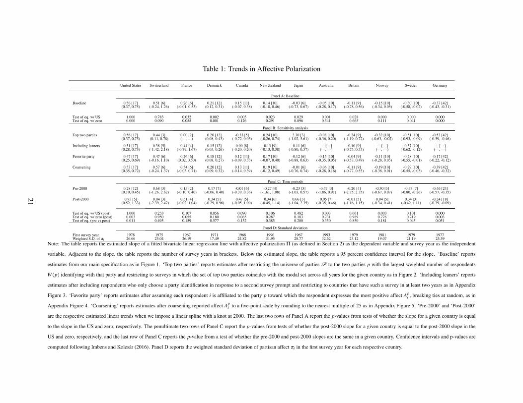
Table 1: Trends in Affective Polarization
United States Switzerland France Denmark Canada New Zealand Japan Australia Britain Norway Sweden Germany
Panel A: Baseline
Baseline 0.56 [17] 0.51 [6] 0.26 [6] 0.21 [12] 0.15 [11] 0.14 [10] -0.03 [6] -0.05 [10] -0.11 [9] -0.15 [10] -0.30 [10] -0.37 [42](0.37, 0.75) (-0.24, 1.26) (-0.01, 0.53) (0.12, 0.31) (-0.07, 0.38) (-0.18, 0.46) (-0.73, 0.67) (-0.28, 0.17) (-0.78, 0.56) (-0.34, 0.05) (-0.58, -0.02) (-0.43, -0.31)
Test of eq. w/ US 1.000 0.783 0.032 0.002 0.005 0.023 0.029 0.001 0.028 0.000 0.000 0.000Test of eq. w/ zero 0.000 0.090 0.055 0.001 0.126 0.291 0.896 0.541 0.665 0.111 0.041 0.000
Panel B: Sensitivity analysis
Top two parties 0.56 [17] 0.44 [3] 0.00 [2] 0.26 [12] -0.33 [5] 0.24 [10] 2.30 [3] -0.08 [10] -0.24 [9] -0.32 [10] -0.51 [10] -0.52 [42](0.37, 0.75) (0.11, 0.78) (---, ---) (0.08, 0.43) (-0.72, 0.05) (-0.26, 0.74) (-1.02, 5.61) (-0.36, 0.20) (-1.19, 0.72) (-0.63, -0.02) (-0.93, -0.09) (-0.59, -0.46)
Including leaners 0.51 [17] 0.38 [5] 0.44 [4] 0.15 [12] 0.00 [8] 0.13 [9] -0.11 [6] --- [---] -0.10 [9] --- [---] -0.37 [10] --- [---](0.28, 0.73) (-1.42, 2.18) (-0.79, 1.67) (0.05, 0.26) (-0.20, 0.20) (-0.13, 0.38) (-0.80, 0.57) (---, ---) (-0.75, 0.55) (---, ---) (-0.62, -0.12) (---, ---)
Favorite party 0.47 [17] 0.47 [6] 0.26 [6] 0.18 [12] 0.12 [11] 0.17 [10] -0.12 [6] -0.15 [10] -0.04 [9] -0.11 [10] -0.28 [10] -0.17 [42](0.25, 0.69) (-0.16, 1.10) (0.02, 0.50) (0.08, 0.27) (-0.09, 0.33) (-0.07, 0.40) (-0.88, 0.63) (-0.35, 0.05) (-0.57, 0.49) (-0.28, 0.05) (-0.55, -0.01) (-0.22, -0.12)
Coarsening 0.53 [17] 0.57 [6] 0.34 [6] 0.20 [12] 0.13 [11] 0.19 [10] -0.01 [6] -0.06 [10] -0.11 [9] -0.19 [10] -0.29 [10] -0.39 [42](0.35, 0.72) (-0.24, 1.37) (-0.03, 0.71) (0.09, 0.32) (-0.14, 0.39) (-0.12, 0.49) (-0.76, 0.74) (-0.28, 0.16) (-0.77, 0.55) (-0.38, 0.01) (-0.55, -0.03) (-0.46, -0.32)
Panel C: Time periods
Pre-2000 0.28 [12] 0.68 [3] 0.15 [2] 0.17 [7] -0.01 [6] -0.27 [4] -0.23 [3] -0.47 [3] -0.20 [4] -0.30 [5] -0.53 [7] -0.46 [24](0.10, 0.45) (-1.26, 2.62) (-0.10, 0.40) (-0.06, 0.40) (-0.39, 0.36) (-1.61, 1.08) (-1.03, 0.57) (-1.86, 0.91) (-2.75, 2.35) (-0.67, 0.07) (-0.80, -0.26) (-0.57, -0.35)
Post-2000 0.93 [5] 0.04 [3] 0.51 [4] 0.34 [5] 0.47 [5] 0.34 [6] 0.66 [3] 0.05 [7] -0.01 [5] 0.04 [5] 0.34 [3] -0.24 [18](0.52, 1.33) (-2.39, 2.47) (-0.02, 1.04) (-0.29, 0.96) (-0.05, 1.00) (-0.45, 1.14) (-1.04, 2.35) (-0.35, 0.46) (-1.16, 1.15) (-0.34, 0.41) (-0.42, 1.11) (-0.39, -0.09)
Test of eq. w/ US (post) 1.000 0.253 0.107 0.056 0.090 0.106 0.482 0.003 0.061 0.003 0.101 0.000Test of eq. w/ zero (post) 0.003 0.950 0.055 0.180 0.065 0.287 0.183 0.731 0.989 0.776 0.219 0.003Test of eq. (pre vs post) 0.011 0.495 0.159 0.577 0.132 0.385 0.200 0.350 0.850 0.181 0.045 0.051
Panel D: Standard deviation
First survey year 1978 1975 1967 1971 1968 1990 1967 1993 1979 1981 1979 1977Weighted S.D. of πi 26.66 23.04 26.19 17.49 24.82 31.95 28.77 32.62 23.12 19.07 21.19 25.39
Note: The table reports the estimated slope of a fitted bivariate linear regression line with affective polarization Π (as defined in Section 2) as the dependent variable and survey year as the independent
variable. Adjacent to the slope, the table reports the number of survey years in brackets. Below the estimated slope, the table reports a 95 percent confidence interval for the slope. ‘Baseline’ reports
estimates from our main specification as in Figure 1. ‘Top two parties’ reports estimates after restricting the universe of parties P to the two parties p with the largest weighted number of respondents
W (p) identifying with that party and restricting to surveys in which the set of top two parties coincides with the modal set across all years for the given country as in Figure 2. ‘Including leaners’ reports
estimates after including respondents who only choose a party identification in response to a second survey prompt and restricting to countries that have such a survey in at least two years as in Appendix
Figure 3. ‘Favorite party’ reports estimates after assuming each respondent i is affiliated to the party p toward which the respondent expresses the most positive affect Api , breaking ties at random, as in
Appendix Figure 4. ‘Coarsening’ reports estimates after coarsening reported affect Api to a five-point scale by rounding to the nearest multiple of 25 as in Appendix Figure 5. ‘Pre-2000’ and ‘Post-2000’
are the respective estimated linear trends when we impose a linear spline with a knot at 2000. The last two rows of Panel A report the p-values from tests of whether the slope for a given country is equal
to the slope in the US and zero, respectively. The penultimate two rows of Panel C report the p-values from tests of whether the post-2000 slope for a given country is equal to the post-2000 slope in the
US and zero, respectively, and the last row of Panel C reports the p-value from a test of whether the pre-2000 and post-2000 slopes are the same in a given country. Confidence intervals and p-values are
computed following Imbens and Kolesar (2016). Panel D reports the weighted standard deviation of partisan affect πi in the first survey year for each respective country.
21

A Appendix for Online Publication
A.1 Trends in Party Affiliation
Appendix Figure 1: Trends in Party Affiliation
Panel A: Share of Respondents Stating a Party Affiliation
0.00
0.25
0.50
0.75
1.00
1960 1980 2000 2020
Pro
port
ion
United States
0.00
0.25
0.50
0.75
1.00
1960 1980 2000 2020
Switzerland
0.00
0.25
0.50
0.75
1.00
1960 1980 2000 2020
France
0.00
0.25
0.50
0.75
1.00
1960 1980 2000 2020
Denmark
0.00
0.25
0.50
0.75
1.00
1960 1980 2000 2020
Canada
0.00
0.25
0.50
0.75
1.00
1960 1980 2000 2020
New Zealand
0.00
0.25
0.50
0.75
1.00
1960 1980 2000 2020
Japan
0.00
0.25
0.50
0.75
1.00
1960 1980 2000 2020
Australia
0.00
0.25
0.50
0.75
1.00
1960 1980 2000 2020
Britain
0.00
0.25
0.50
0.75
1.00
1960 1980 2000 2020
Norway
0.00
0.25
0.50
0.75
1.00
1960 1980 2000 2020
Sweden
0.00
0.25
0.50
0.75
1.00
1960 1980 2000 2020
Germany
Panel B: Share of Affiliates Affiliated with Top Two Parties
0.00
0.25
0.50
0.75
1.00
1960 1980 2000 2020
Pro
port
ion
United States
0.00
0.25
0.50
0.75
1.00
1960 1980 2000 2020
Switzerland
0.00
0.25
0.50
0.75
1.00
1960 1980 2000 2020
France
0.00
0.25
0.50
0.75
1.00
1960 1980 2000 2020
Denmark
0.00
0.25
0.50
0.75
1.00
1960 1980 2000 2020
Canada
0.00
0.25
0.50
0.75
1.00
1960 1980 2000 2020
New Zealand
0.00
0.25
0.50
0.75
1.00
1960 1980 2000 2020
Japan
0.00
0.25
0.50
0.75
1.00
1960 1980 2000 2020
Australia
0.00
0.25
0.50
0.75
1.00
1960 1980 2000 2020
Britain
0.00
0.25
0.50
0.75
1.00
1960 1980 2000 2020
Norway
0.00
0.25
0.50
0.75
1.00
1960 1980 2000 2020
Sweden
0.00
0.25
0.50
0.75
1.00
1960 1980 2000 2020
Germany
Note: Panel A shows the weighted number of affiliates expressed as a share of the weighted number of respondents.Panel B shows the weighted number of respondents affiliated with the top two parties, expressed as a share of theweighted number of affiliates. In both panels, the weighted number of affiliates is the weighted number of respondentswho state an affiliation to a party about which an affect question is asked in at least one survey for the given country.In Panel B, distinct shapes are used to indicate sets of survey years for which the top two parties are the same.
22

A.2 Sensitivity Analysis
Appendix Figure 2: Trends in Own-Party and Other-Party Affect by Country
Slope: −0.06(−0.16, 0.03)
Slope: −0.62(−0.79, −0.46)
102030405060708090
100110
1980 2000 2020
Affe
ct
Party
Own
Other
USSlope: 0.29(−0.23, 0.81)
Slope: −0.22(−0.50, 0.05)20
30405060708090
100110120
1980 2000 2020
Party
Own
Other
SwitzerlandSlope: 0.11(−0.02, 0.23)
Slope: −0.15(−0.38, 0.08)10
2030405060708090
100110
1980 2000 2020
Party
Own
Other
France
Slope: −0.15(−0.24, −0.06)
Slope: −0.36(−0.45, −0.28)
30405060708090
100110120
1980 2000 2020
Party
Own
Other
DenmarkSlope: −0.02(−0.26, 0.21)
Slope: −0.18(−0.24, −0.11)10
2030405060708090
100110
1980 2000 2020
Party
Own
Other
CanadaSlope: 0.26(0.02, 0.51)
Slope: 0.12(−0.16, 0.40)
2030405060708090
100110120
1980 2000 2020
Party
Own
Other
New Zealand
Slope: −0.07(−0.79, 0.64)
Slope: −0.05(−0.18, 0.08)
2030405060708090
100110120
1980 2000 2020
Party
Own
Other
JapanSlope: −0.14(−0.31, 0.02)
Slope: −0.09(−0.42, 0.25)
2030405060708090
100110
1980 2000 2020
Party
Own
Other
AustraliaSlope: −0.31(−0.46, −0.15)
Slope: −0.20(−0.75, 0.36)10
2030405060708090
100110
1980 2000 2020
Party
Own
Other
Britain
Slope: −0.06(−0.18, 0.06)
Slope: 0.08(−0.05, 0.21)20
30405060708090
100110120
1980 2000 2020
Party
Own
Other
NorwaySlope: −0.11(−0.26, 0.05)
Slope: 0.19(−0.02, 0.40)20
30405060708090
100110120
1980 2000 2020
Party
Own
Other
SwedenSlope: −0.17(−0.27, −0.08)
Slope: 0.20(0.12, 0.28)
30405060708090
100110120
1980 2000 2020
Party
Own
Other
Germany
Note: The plot decomposes affective polarization Π into own-party affect (black circles) and other-party affect (red triangles). Following thenotation in Section 2, own-party affect is defined as the weighted average of Ap(i)
i , whereas other-party affect is defined as the weighted average of
∑p′∈Pi\p(i)
W (p′)W (Pi)−W (p(i))
Ap′i .
Thus, affective polarization Π is equal to the difference between own-party affect and other-party affect. In each plot, one point represents onesurvey. The solid lines display fitted bivariate linear regression lines with affect as the dependent variable and survey year as the independentvariable. Each plot reports the estimated slopes (change per year) and the corresponding 95 percent confidence intervals computed followingImbens and Kolesar (2016).
23

Appendix Figure 3: Trends in Affective Polarization by Country – Including Leaners
Slope: 0.51(0.28, 0.73)
25
30
35
40
45
50
55
60
65
1980 2000 2020
Affe
ctiv
e po
lariz
atio
n
Original response scaling
favorable and warm (0−100)
USSlope: 0.38(−1.42, 2.18)
25
30
35
40
45
50
55
60
65
1980 2000 2020
Original response scaling
like (0−10)
like (0−100)
sympathy (0−10)
SwitzerlandSlope: 0.44(−0.79, 1.67)
30
35
40
45
50
55
60
65
70
1980 2000 2020
Original response scaling
like (0−10)
France
Slope: 0.15(0.05, 0.26)
25
30
35
40
45
50
55
60
65
1980 2000 2020
Original response scaling
like (0−10)
like (−50 to 50)
like (−100 to 100)
like (−100 to 100 by 20)
DenmarkSlope: 0.00(−0.20, 0.20)
15
20
25
30
35
40
45
50
55
1980 2000 2020
Original response scaling
favourable (0−100)
like (0−100)
warm (0−100)
CanadaSlope: 0.13(−0.13, 0.38)
30
35
40
45
50
55
60
65
70
1980 2000 2020
Original response scaling
like (0−10)
support−oppose (1−5)
New Zealand
Slope: −0.11(−0.80, 0.57)
20
25
30
35
40
45
50
55
60
1980 2000 2020
Original response scaling
like (0−10)
like (0−100)
like (1−5)
Japan
Only one survey with leaners question
AustraliaSlope: −0.10(−0.75, 0.55)
25
30
35
40
45
50
55
60
65
1980 2000 2020
Original response scaling
like (0−10)
favour−against (1−5)
Britain
No leaners question
NorwaySlope: −0.37(−0.62, −0.12)
30
35
40
45
50
55
60
65
70
1980 2000 2020
Original response scaling
like (−5 to 5)
Sweden
No leaners question
Germany
Note: The plot shows estimates of affective polarization Π as defined in Section 2. In contrast to our baselineestimates, we include leaners in the sample. Leaners are respondents who only choose a party identificationin response to a second survey prompt. We include only surveys that have a second prompt, and onlycountries that have such a survey in at least two years. In each plot, one point represents one survey. Thered line displays a fitted bivariate linear regression line with affective polarization as the dependent variableand survey year as the independent variable. Each plot reports the estimated slope (change per year) and thecorresponding 95 percent confidence interval following Imbens and Kolesar (2016).
24

Appendix Figure 4: Trends in Affective Polarization by Country – Favorite Party
Slope: 0.47(0.25, 0.69)
25
30
35
40
45
50
55
60
1980 2000 2020
Affe
ctiv
e po
lariz
atio
n
Original response scaling
favorable and warm (0−100)
USSlope: 0.47(−0.16, 1.10)
25
30
35
40
45
50
55
60
1980 2000 2020
Original response scaling
like (0−10)
like (0−100)
sympathy (0−10)
SwitzerlandSlope: 0.26(0.02, 0.50)
25
30
35
40
45
50
55
60
65
1980 2000 2020
Original response scaling
like (0−10)
sympathy (0−100)
close−negative feelings (0−100)
France
Slope: 0.18(0.08, 0.27)
30
35
40
45
50
55
60
65
1980 2000 2020
Original response scaling
like (0−10)
like (−50 to 50)
like (−100 to 100)
like (−100 to 100 by 20)
DenmarkSlope: 0.12(−0.09, 0.33)
20
25
30
35
40
45
50
55
60
1980 2000 2020
Original response scaling
favourable (0−100)
like (0−100)
warm (0−100)
CanadaSlope: 0.17(−0.07, 0.40)
30
35
40
45
50
55
60
65
70
1980 2000 2020
Original response scaling
like (0−10)
support−oppose (1−5)
New Zealand
Slope: −0.12(−0.88, 0.63)
20
25
30
35
40
45
50
55
60
1980 2000 2020
Original response scaling
like (0−10)
like (0−100)
like (1−5)
JapanSlope: −0.15(−0.35, 0.05)
30
35
40
45
50
55
60
65
70
1980 2000 2020
Original response scaling
like (0−10)
favourable (0−10)
AustraliaSlope: −0.04(−0.57, 0.49)
25
30
35
40
45
50
55
60
65
1980 2000 2020
Original response scaling
like (0−10)
favour−against (1−5)
Britain
Slope: −0.11(−0.28, 0.05)
25
30
35
40
45
50
55
60
65
1980 2000 2020
Original response scaling
like (0−10)
like (0−100)
NorwaySlope: −0.28(−0.55, −0.01)
30
35
40
45
50
55
60
65
1980 2000 2020
Original response scaling
like (−5 to 5)
SwedenSlope: −0.17(−0.22, −0.12)
20
25
30
35
40
45
50
55
60
1980 2000 2020
Original response scaling
think highly (−5 to 5)
Germany
Note: The plot shows estimates of affective polarization Π as defined in Section 2. In contrast to our baselineestimates, we assume that each respondent i is affiliated to the party p toward which the respondent expressesthe most positive affect Ap
i , breaking ties at random. In each plot, one point represents one survey. The redline displays a fitted bivariate linear regression line with affective polarization as the dependent variable andsurvey year as the independent variable. Each plot reports the estimated slope (change per year) and thecorresponding 95 percent confidence interval computed following Imbens and Kolesar (2016).
25

Appendix Figure 5: Trends in Affective Polarization by Country – Coarsening Reported Affect
Slope: 0.53(0.35, 0.72)
25
30
35
40
45
50
55
60
65
1980 2000 2020
Affe
ctiv
e po
lariz
atio
n
Original response scaling
favorable and warm (0−100)
USSlope: 0.57(−0.24, 1.37)
30
35
40
45
50
55
60
65
70
1980 2000 2020
Original response scaling
like (0−10)
like (0−100)
sympathy (0−10)
SwitzerlandSlope: 0.34(−0.03, 0.71)
30
35
40
45
50
55
60
65
70
1980 2000 2020
Original response scaling
like (0−10)
sympathy (0−100)
close−negative feelings (0−100)
France
Slope: 0.20(0.09, 0.32)
35
40
45
50
55
60
65
70
1980 2000 2020
Original response scaling
like (0−10)
like (−50 to 50)
like (−100 to 100)
like (−100 to 100 by 20)
DenmarkSlope: 0.13(−0.14, 0.39)
20
25
30
35
40
45
50
55
1980 2000 2020
Original response scaling
favourable (0−100)
like (0−100)
warm (0−100)
CanadaSlope: 0.19(−0.12, 0.49)
35
40
45
50
55
60
65
70
75
1980 2000 2020
Original response scaling
like (0−10)
support−oppose (1−5)
New Zealand
Slope: −0.01(−0.76, 0.74)
25
30
35
40
45
50
55
60
1980 2000 2020
Original response scaling
like (0−10)
like (0−100)
like (1−5)
JapanSlope: −0.06(−0.28, 0.16)
35
40
45
50
55
60
65
70
75
1980 2000 2020
Original response scaling
like (0−10)
favourable (0−10)
AustraliaSlope: −0.11(−0.77, 0.55)
30
35
40
45
50
55
60
65
1980 2000 2020
Original response scaling
like (0−10)
favour−against (1−5)
Britain
Slope: −0.19(−0.38, 0.01)
30
35
40
45
50
55
60
65
70
1980 2000 2020
Original response scaling
like (0−10)
like (0−100)
NorwaySlope: −0.29(−0.55, −0.03)
40
45
50
55
60
65
70
75
80
1980 2000 2020
Original response scaling
like (−5 to 5)
SwedenSlope: −0.39(−0.46, −0.32)
20
25
30
35
40
45
50
55
60
1980 2000 2020
Original response scaling
think highly (−5 to 5)
Germany
Note: The plot shows estimates of affective polarization Π as defined in Section 2. In contrast to our baselineestimates, we coarsen reported affect Ap
i to a five-point scale by rounding to the nearest multiple of 25. Ineach plot, one point represents one survey. The red line displays a fitted bivariate linear regression linewith affective polarization as the dependent variable and survey year as the independent variable. Each plotreports the estimated slope (change per year) and the corresponding 95 percent confidence interval computedfollowing Imbens and Kolesar (2016).
26
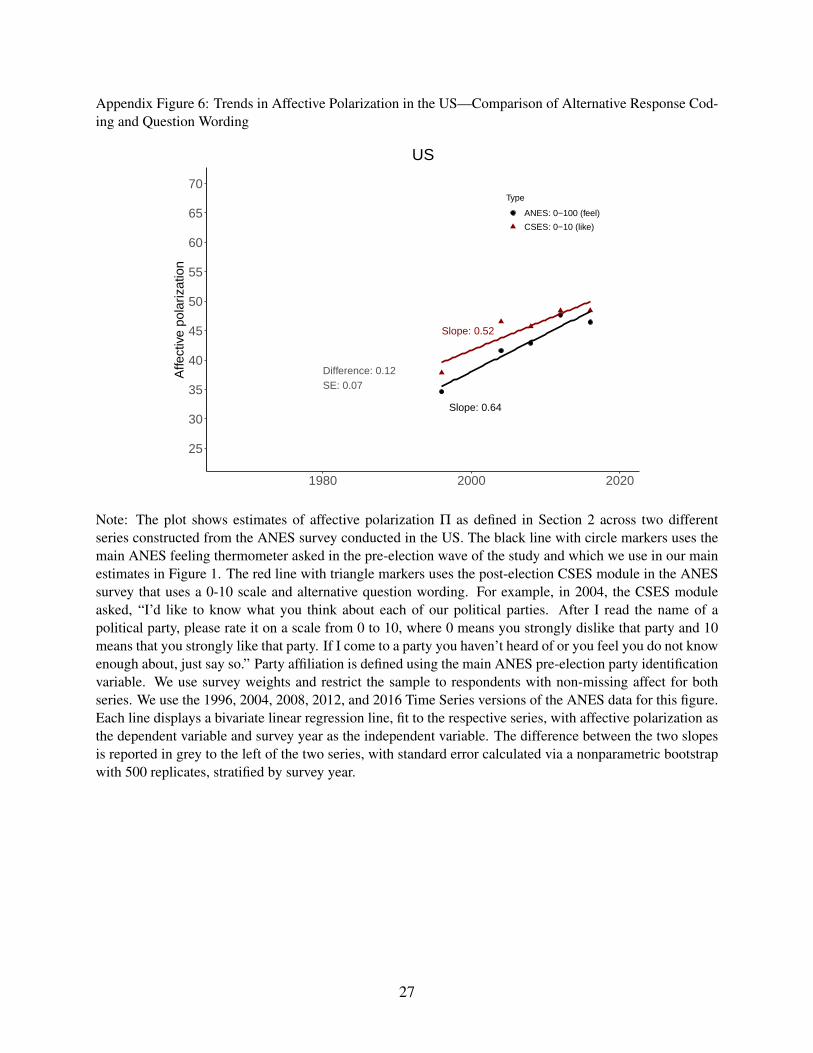
Appendix Figure 6: Trends in Affective Polarization in the US—Comparison of Alternative Response Cod-ing and Question Wording
Slope: 0.64
Slope: 0.52
Difference: 0.12SE: 0.07
25
30
35
40
45
50
55
60
65
70
1980 2000 2020
Affe
ctiv
e po
lariz
atio
nType
ANES: 0−100 (feel)
CSES: 0−10 (like)
US
Note: The plot shows estimates of affective polarization Π as defined in Section 2 across two differentseries constructed from the ANES survey conducted in the US. The black line with circle markers uses themain ANES feeling thermometer asked in the pre-election wave of the study and which we use in our mainestimates in Figure 1. The red line with triangle markers uses the post-election CSES module in the ANESsurvey that uses a 0-10 scale and alternative question wording. For example, in 2004, the CSES moduleasked, “I’d like to know what you think about each of our political parties. After I read the name of apolitical party, please rate it on a scale from 0 to 10, where 0 means you strongly dislike that party and 10means that you strongly like that party. If I come to a party you haven’t heard of or you feel you do not knowenough about, just say so.” Party affiliation is defined using the main ANES pre-election party identificationvariable. We use survey weights and restrict the sample to respondents with non-missing affect for bothseries. We use the 1996, 2004, 2008, 2012, and 2016 Time Series versions of the ANES data for this figure.Each line displays a bivariate linear regression line, fit to the respective series, with affective polarization asthe dependent variable and survey year as the independent variable. The difference between the two slopesis reported in grey to the left of the two series, with standard error calculated via a nonparametric bootstrapwith 500 replicates, stratified by survey year.
27

Appendix Figure 7: Comparing Measured Trends to CSES
25303540455055606570
1980 2000 2020
Affe
ctiv
e po
lariz
atio
n
Type
CSES
Our Main Series
United States
2530354045505560657075
1980 2000 2020
Type
CSES
Our Main Series
Switzerland
30354045505560657075
1980 2000 2020
Type
CSES
Our Main Series
France
2530354045505560657075
1980 2000 2020
Type
CSES
Our Main Series
Denmark
1015202530354045505560
1980 2000 2020
Type
CSES
Our Main Series
Canada
2530354045505560657075
1980 2000 2020
Type
CSES
Our Main Series
New Zealand
15202530354045505560
1980 2000 2020
Type
CSES
Our Main Series
Japan
25303540455055606570
1980 2000 2020
Type
CSES
Our Main Series
Australia
1520253035404550556065
1980 2000 2020
Type
CSES
Our Main Series
Britain
20253035404550556065
1980 2000 2020
Type
CSES
Our Main Series
Norway
25303540455055606570
1980 2000 2020
Type
CSES
Our Main Series
Sweden
10152025303540455055
1980 2000 2020
Type
CSES
Our Main Series
Germany
Note: The plot shows our estimates of affective polarization Π as defined in Section 2 for our main series as well as for data from the ComparativeStudy of Electoral Systems (CSES). In some cases, our main series uses the CSES data directly: Switzerland (2003), France (post-2000), and Japan(post-1990). In other cases, our main data provider and the CSES are often collaborators using the same sample of respondents. In each plot, onepoint represents one survey. We normalize the level of the CSES series so that the first CSES survey aligns with the level of the corresponding (orpreceeding) year in our main series. The CSES series is shifted left by 1/3 years for ease of visualization, and we restrict the CSES data to WestGermany for consistency with our main series.
28

A.3 Plots of Potential Explanatory Factors
Appendix Figure 8: Potential Explanatory Factors – Plots
Panel A: Affective Polarization
Slope: 0.56
(0.37, 0.75)
24
30
36
42
48
54
60
1980 2000 2020
Affe
ctiv
e po
lariz
atio
n
USSlope: 0.51
(−0.24, 1.26)
24
30
36
42
48
54
60
1980 2000 2020
SwitzerlandSlope: 0.26
(−0.01, 0.53)
30
36
42
48
54
60
66
72
1980 2000 2020
FranceSlope: 0.21
(0.12, 0.31)
36
42
48
54
60
66
72
1980 2000 2020
DenmarkSlope: 0.15
(−0.07, 0.38)
18
24
30
36
42
48
54
1980 2000 2020
CanadaSlope: 0.14
(−0.18, 0.46)
36
42
48
54
60
66
72
1980 2000 2020
New ZealandSlope: −0.03
(−0.73, 0.67)
24
30
36
42
48
54
60
1980 2000 2020
JapanSlope: −0.05
(−0.28, 0.17)
36
42
48
54
60
66
72
1980 2000 2020
AustraliaSlope: −0.11
(−0.78, 0.56)
24
30
36
42
48
54
60
1980 2000 2020
BritainSlope: −0.15
(−0.34, 0.05)
30
36
42
48
54
60
66
1980 2000 2020
NorwaySlope: −0.30
(−0.58, −0.02)
36
42
48
54
60
66
72
78
1980 2000 2020
SwedenSlope: −0.37
(−0.43, −0.31)
18
24
30
36
42
48
54
1980 2000 2020
Germany
Panel B: Trade Share of GDP
Slope: 0.35
(0.30, 0.39)
0
12
24
36
48
60
72
1980 2000 2020
Trad
e sh
are
of G
DP
USSlope: 0.85
(0.69, 1.01)
72
84
96
108
120
132
144
1980 2000 2020
SwitzerlandSlope: 0.63
(0.60, 0.67)
12
24
36
48
60
72
84
1980 2000 2020
FranceSlope: 1.01
(0.92, 1.11)
48
60
72
84
96
108
120
1980 2000 2020
DenmarkSlope: 0.63
(0.53, 0.73)
24
36
48
60
72
84
96
1980 2000 2020
CanadaSlope: 0.13
(0.03, 0.24)
36
48
60
72
84
96
108
1980 2000 2020
New ZealandSlope: 0.24
(0.15, 0.34)
12
24
36
48
60
72
84
1980 2000 2020
JapanSlope: 0.35
(0.32, 0.39)
12
24
36
48
60
72
84
1980 2000 2020
AustraliaSlope: 0.23
(0.13, 0.33)
36
48
60
72
84
96
108
1980 2000 2020
BritainSlope: −0.15
(−0.22, −0.08)
60
72
84
96
108
120
132
1980 2000 2020
NorwaySlope: 0.93
(0.87, 1.00)
24
36
48
60
72
84
96
108
1980 2000 2020
SwedenSlope: 1.25
(1.16, 1.35)
24
36
48
60
72
84
96
1980 2000 2020
Germany
Panel C: Inequality (Gini)
Slope: 0.09
(0.04, 0.14)
33
36
39
42
45
48
51
1980 2000 2020
Ineq
ualit
y (G
ini)
USSlope: −0.09
(−0.17, −0.00)
30
33
36
39
42
45
1980 2000 2020
SwitzerlandSlope: −0.19
(−0.24, −0.14)
27
30
33
36
39
42
1980 2000 2020
FranceSlope: 0.16
(0.00, 0.31)
21
24
27
30
33
36
1980 2000 2020
DenmarkSlope: 0.11
(0.08, 0.13)
27
30
33
36
39
42
1980 2000 2020
CanadaSlope: 0.22
(0.13, 0.30)
24
27
30
33
36
39
1980 2000 2020
New ZealandSlope: 0.05
(0.01, 0.09)
21
24
27
30
33
36
1980 2000 2020
JapanSlope: 0.15
(0.10, 0.20)
24
27
30
33
36
39
42
1980 2000 2020
AustraliaSlope: 0.25
(0.21, 0.28)
21
24
27
30
33
36
1980 2000 2020
BritainSlope: 0.15
(0.10, 0.20)
18
21
24
27
30
33
36
1980 2000 2020
NorwaySlope: 0.33
(0.28, 0.38)
18
21
24
27
30
33
36
1980 2000 2020
SwedenSlope: 0.07
(−0.03, 0.17)
21
24
27
30
33
36
1980 2000 2020
Germany
Panel D: Internet PenetrationSlope: 3.37
(2.98, 3.77)
−21
0
21
42
63
84
105
1980 2000 2020
Inte
rnet
pen
etra
tion
USSlope: 3.90
(3.37, 4.42)
−21
0
21
42
63
84
105
1980 2000 2020
SwitzerlandSlope: 3.75
(3.32, 4.18)
−21
0
21
42
63
84
105
1980 2000 2020
FranceSlope: 4.21
(3.66, 4.77)
−21
0
21
42
63
84
105
1980 2000 2020
DenmarkSlope: 4.04
(3.57, 4.50)
−21
0
21
42
63
84
105
1980 2000 2020
CanadaSlope: 3.90
(3.42, 4.38)
−21
0
21
42
63
84
105
1980 2000 2020
New ZealandSlope: 4.12
(3.71, 4.52)
−21
0
21
42
63
84
105
1980 2000 2020
JapanSlope: 3.80
(3.40, 4.20)
−21
0
21
42
63
84
105
1980 2000 2020
AustraliaSlope: 4.09
(3.60, 4.59)
−21
0
21
42
63
84
105
1980 2000 2020
BritainSlope: 4.03
(3.42, 4.65)
−21
0
21
42
63
84
105
1980 2000 2020
NorwaySlope: 4.05
(3.35, 4.74)
−21
0
21
42
63
84
105
1980 2000 2020
SwedenSlope: 3.87
(3.39, 4.36)
−21
0
21
42
63
84
105
1980 2000 2020
Germany
Note: Countries are sorted from left to right in descending order of the estimated linear time trend of affective polarization. Panel A plots the measure of affectivepolarization along with the estimated linear time trend for each country; Panel B plots the trade share of GDP in each country; Panel C plots the Gini coefficient foreach country; and Panel D plots the share of households with internet access in each country. See Appendix A.7 for additional details on data sources and construction.Each plot reports the estimated slope (change per year) and the corresponding 95 percent confidence interval computed following Imbens and Kolesar (2016). Plotswith an asterisk after the country name indicate the countries excluded from the computations in Figure 3 for each respective variable.
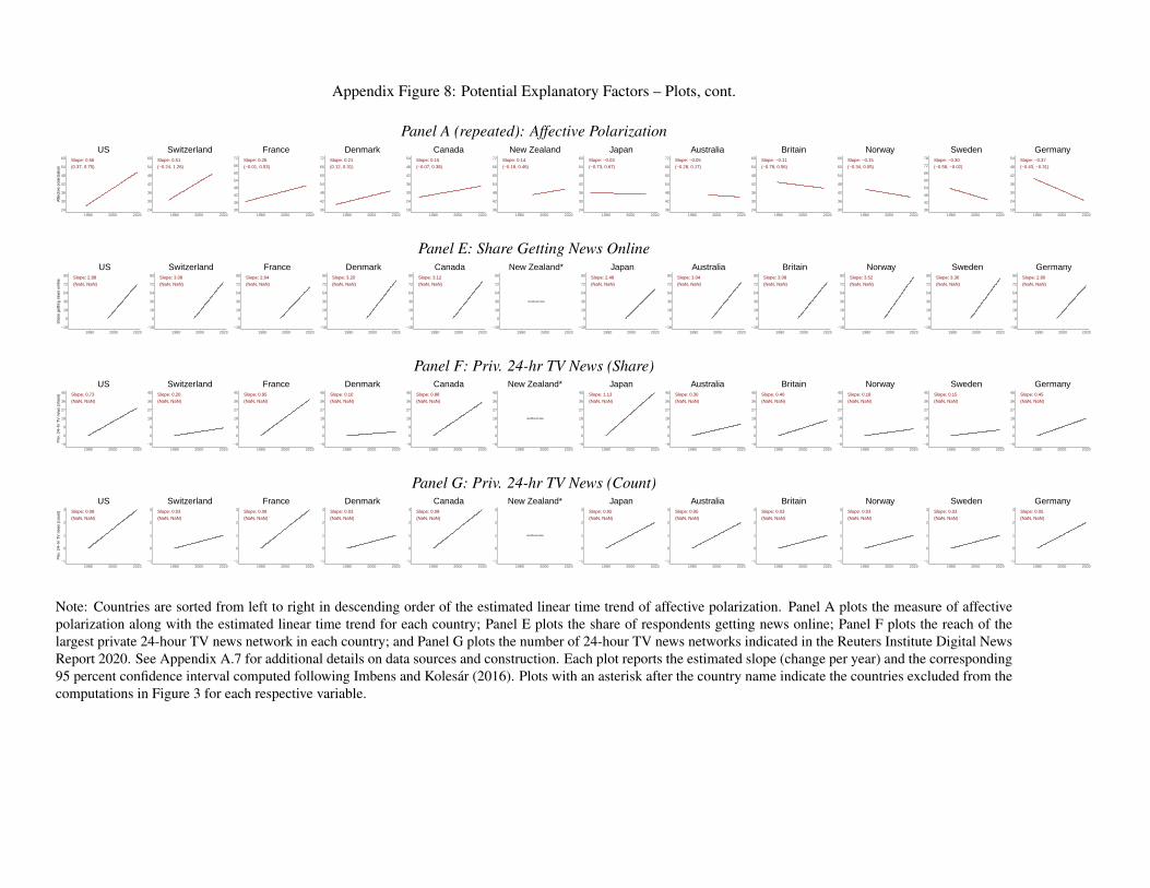
Appendix Figure 8: Potential Explanatory Factors – Plots, cont.
Panel A (repeated): Affective Polarization
Slope: 0.56
(0.37, 0.75)
24
30
36
42
48
54
60
1980 2000 2020
Affe
ctiv
e po
lariz
atio
n
USSlope: 0.51
(−0.24, 1.26)
24
30
36
42
48
54
60
1980 2000 2020
SwitzerlandSlope: 0.26
(−0.01, 0.53)
30
36
42
48
54
60
66
72
1980 2000 2020
FranceSlope: 0.21
(0.12, 0.31)
36
42
48
54
60
66
72
1980 2000 2020
DenmarkSlope: 0.15
(−0.07, 0.38)
18
24
30
36
42
48
54
1980 2000 2020
CanadaSlope: 0.14
(−0.18, 0.46)
36
42
48
54
60
66
72
1980 2000 2020
New ZealandSlope: −0.03
(−0.73, 0.67)
24
30
36
42
48
54
60
1980 2000 2020
JapanSlope: −0.05
(−0.28, 0.17)
36
42
48
54
60
66
72
1980 2000 2020
AustraliaSlope: −0.11
(−0.78, 0.56)
24
30
36
42
48
54
60
1980 2000 2020
BritainSlope: −0.15
(−0.34, 0.05)
30
36
42
48
54
60
66
1980 2000 2020
NorwaySlope: −0.30
(−0.58, −0.02)
36
42
48
54
60
66
72
78
1980 2000 2020
SwedenSlope: −0.37
(−0.43, −0.31)
18
24
30
36
42
48
54
1980 2000 2020
Germany
Panel E: Share Getting News Online
Slope: 2.88
(NaN, NaN)
−18
0
18
36
54
72
90
1980 2000 2020
Sha
re g
ettin
g ne
ws
onlin
e
USSlope: 3.08
(NaN, NaN)
−18
0
18
36
54
72
90
1980 2000 2020
SwitzerlandSlope: 2.64
(NaN, NaN)
−18
0
18
36
54
72
90
1980 2000 2020
FranceSlope: 3.20
(NaN, NaN)
−18
0
18
36
54
72
90
1980 2000 2020
DenmarkSlope: 3.12
(NaN, NaN)
−18
0
18
36
54
72
90
1980 2000 2020
Canada
Insufficient data
−18
0
18
36
54
72
90
1980 2000 2020
New Zealand*Slope: 2.48
(NaN, NaN)
−18
0
18
36
54
72
90
1980 2000 2020
JapanSlope: 3.04
(NaN, NaN)
−18
0
18
36
54
72
90
1980 2000 2020
AustraliaSlope: 3.08
(NaN, NaN)
−18
0
18
36
54
72
90
1980 2000 2020
BritainSlope: 3.52
(NaN, NaN)
−18
0
18
36
54
72
90
1980 2000 2020
NorwaySlope: 3.36
(NaN, NaN)
−18
0
18
36
54
72
90
1980 2000 2020
SwedenSlope: 2.80
(NaN, NaN)
−18
0
18
36
54
72
90
1980 2000 2020
Germany
Panel F: Priv. 24-hr TV News (Share)
Slope: 0.73
(NaN, NaN)
−9
0
9
18
27
36
45
1980 2000 2020
Priv
. 24−
hr T
V n
ews
(sha
re)
USSlope: 0.20
(NaN, NaN)
−9
0
9
18
27
36
45
1980 2000 2020
SwitzerlandSlope: 0.95
(NaN, NaN)
−9
0
9
18
27
36
45
1980 2000 2020
FranceSlope: 0.10
(NaN, NaN)
−9
0
9
18
27
36
45
1980 2000 2020
DenmarkSlope: 0.88
(NaN, NaN)
−9
0
9
18
27
36
45
1980 2000 2020
Canada
Insufficient data
−9
0
9
18
27
36
45
1980 2000 2020
New Zealand*Slope: 1.13
(NaN, NaN)
−9
0
9
18
27
36
45
1980 2000 2020
JapanSlope: 0.30
(NaN, NaN)
−9
0
9
18
27
36
45
1980 2000 2020
AustraliaSlope: 0.40
(NaN, NaN)
−9
0
9
18
27
36
45
1980 2000 2020
BritainSlope: 0.18
(NaN, NaN)
−9
0
9
18
27
36
45
1980 2000 2020
NorwaySlope: 0.15
(NaN, NaN)
−9
0
9
18
27
36
45
1980 2000 2020
SwedenSlope: 0.45
(NaN, NaN)
−9
0
9
18
27
36
45
1980 2000 2020
Germany
Panel G: Priv. 24-hr TV News (Count)
Slope: 0.08
(NaN, NaN)
−1
0
1
2
3
1980 2000 2020
Priv
. 24−
hr T
V n
ews
(cou
nt)
USSlope: 0.03
(NaN, NaN)
−1
0
1
2
3
1980 2000 2020
SwitzerlandSlope: 0.08
(NaN, NaN)
−1
0
1
2
3
1980 2000 2020
FranceSlope: 0.03
(NaN, NaN)
−1
0
1
2
3
1980 2000 2020
DenmarkSlope: 0.08
(NaN, NaN)
−1
0
1
2
3
1980 2000 2020
Canada
Insufficient data
−1
0
1
2
3
1980 2000 2020
New Zealand*Slope: 0.05
(NaN, NaN)
−1
0
1
2
3
1980 2000 2020
JapanSlope: 0.05
(NaN, NaN)
−1
0
1
2
3
1980 2000 2020
AustraliaSlope: 0.03
(NaN, NaN)
−1
0
1
2
3
1980 2000 2020
BritainSlope: 0.03
(NaN, NaN)
−1
0
1
2
3
1980 2000 2020
NorwaySlope: 0.03
(NaN, NaN)
−1
0
1
2
3
1980 2000 2020
SwedenSlope: 0.05
(NaN, NaN)
−1
0
1
2
3
1980 2000 2020
Germany
Note: Countries are sorted from left to right in descending order of the estimated linear time trend of affective polarization. Panel A plots the measure of affectivepolarization along with the estimated linear time trend for each country; Panel E plots the share of respondents getting news online; Panel F plots the reach of thelargest private 24-hour TV news network in each country; and Panel G plots the number of 24-hour TV news networks indicated in the Reuters Institute Digital NewsReport 2020. See Appendix A.7 for additional details on data sources and construction. Each plot reports the estimated slope (change per year) and the corresponding95 percent confidence interval computed following Imbens and Kolesar (2016). Plots with an asterisk after the country name indicate the countries excluded from thecomputations in Figure 3 for each respective variable.

Appendix Figure 8: Potential Explanatory Factors – Plots, cont.
Panel A (repeated): Affective Polarization
Slope: 0.56
(0.37, 0.75)
24
30
36
42
48
54
60
1980 2000 2020
Affe
ctiv
e po
lariz
atio
n
USSlope: 0.51
(−0.24, 1.26)
24
30
36
42
48
54
60
1980 2000 2020
SwitzerlandSlope: 0.26
(−0.01, 0.53)
30
36
42
48
54
60
66
72
1980 2000 2020
FranceSlope: 0.21
(0.12, 0.31)
36
42
48
54
60
66
72
1980 2000 2020
DenmarkSlope: 0.15
(−0.07, 0.38)
18
24
30
36
42
48
54
1980 2000 2020
CanadaSlope: 0.14
(−0.18, 0.46)
36
42
48
54
60
66
72
1980 2000 2020
New ZealandSlope: −0.03
(−0.73, 0.67)
24
30
36
42
48
54
60
1980 2000 2020
JapanSlope: −0.05
(−0.28, 0.17)
36
42
48
54
60
66
72
1980 2000 2020
AustraliaSlope: −0.11
(−0.78, 0.56)
24
30
36
42
48
54
60
1980 2000 2020
BritainSlope: −0.15
(−0.34, 0.05)
30
36
42
48
54
60
66
1980 2000 2020
NorwaySlope: −0.30
(−0.58, −0.02)
36
42
48
54
60
66
72
78
1980 2000 2020
SwedenSlope: −0.37
(−0.43, −0.31)
18
24
30
36
42
48
54
1980 2000 2020
Germany
Panel H: Foreign-born Share
Slope: 0.20
(0.18, 0.22)
6
9
12
15
18
21
1980 2000 2020
For
eign
−bo
rn s
hare
USSlope: 0.43
(0.39, 0.47)
18
21
24
27
30
33
36
1980 2000 2020
SwitzerlandSlope: 0.05
(0.03, 0.08)
3
6
9
12
15
18
21
1980 2000 2020
FranceSlope: 0.22
(0.21, 0.24)
0
3
6
9
12
15
18
1980 2000 2020
DenmarkSlope: 0.18
(0.13, 0.22)
12
15
18
21
24
27
30
1980 2000 2020
CanadaSlope: 0.18
(0.12, 0.24)
12
15
18
21
24
27
30
1980 2000 2020
New ZealandSlope: 0.02
(0.01, 0.03)
−3
0
3
6
9
12
15
1980 2000 2020
JapanSlope: 0.26
(0.22, 0.29)
18
21
24
27
30
33
36
1980 2000 2020
AustraliaSlope: 0.30
(0.27, 0.33)
3
6
9
12
15
18
21
1980 2000 2020
BritainSlope: 0.42
(0.37, 0.47)
0
3
6
9
12
15
18
1980 2000 2020
NorwaySlope: 0.34
(0.30, 0.38)
6
9
12
15
18
21
24
1980 2000 2020
SwedenSlope: 0.12
(0.07, 0.18)
9
12
15
18
21
24
27
1980 2000 2020
Germany
Panel I: Non-white ShareSlope: 0.31
(0.29, 0.33)
12
16
20
24
28
32
36
1980 2000 2020
Non
−w
hite
sha
re
USSlope: 0.18
(0.17, 0.18)
4
8
12
16
20
24
28
1980 2000 2020
Switzerland
Insufficient data
−4
0
4
8
12
16
20
24
1980 2000 2020
France*Slope: 0.12
(0.10, 0.14)
−4
0
4
8
12
16
20
24
1980 2000 2020
DenmarkSlope: 0.33
(0.32, 0.34)
8
12
16
20
24
28
32
36
1980 2000 2020
CanadaSlope: 0.32
(0.29, 0.34)
8
12
16
20
24
28
32
1980 2000 2020
New ZealandSlope: 0.00
(−0.00, 0.00)
96
100
104
108
112
116
120
124
1980 2000 2020
JapanSlope: 0.19
(0.17, 0.22)
−4
0
4
8
12
16
20
24
1980 2000 2020
AustraliaSlope: 0.10
(0.09, 0.10)
−4
0
4
8
12
16
20
24
1980 2000 2020
BritainSlope: 0.10
(0.09, 0.11)
−4
0
4
8
12
16
20
24
1980 2000 2020
NorwaySlope: 0.12
(0.12, 0.12)
0
4
8
12
16
20
24
1980 2000 2020
SwedenSlope: 0.07
(0.07, 0.07)
−4
0
4
8
12
16
20
24
1980 2000 2020
Germany
Panel J: Ethnic FractionalizationSlope: 0.45
(0.43, 0.47)
24
30
36
42
48
54
60
1980 2000 2020
Eth
nic
frac
tiona
lizat
ion
USSlope: 0.25
(0.25, 0.25)
18
24
30
36
42
48
54
1980 2000 2020
Switzerland
Insufficient data
−6
0
6
12
18
24
30
36
1980 2000 2020
France*Slope: 0.22
(0.19, 0.25)
−6
0
6
12
18
24
30
36
1980 2000 2020
DenmarkSlope: 0.09
(0.09, 0.09)
66
72
78
84
90
96
102
1980 2000 2020
CanadaSlope: 0.49
(0.46, 0.53)
12
18
24
30
36
42
48
54
1980 2000 2020
New ZealandSlope: 0.01
(0.01, 0.01)
−6
0
6
12
18
24
30
36
1980 2000 2020
JapanSlope: 0.35
(0.31, 0.39)
0
6
12
18
24
30
36
1980 2000 2020
AustraliaSlope: 0.12
(0.11, 0.14)
24
30
36
42
48
54
60
66
1980 2000 2020
BritainSlope: 0.19
(0.17, 0.21)
0
6
12
18
24
30
36
1980 2000 2020
NorwaySlope: 0.18
(0.18, 0.19)
6
12
18
24
30
36
42
1980 2000 2020
SwedenSlope: −0.26
(−0.65, 0.12)
6
12
18
24
30
36
42
1980 2000 2020
Germany
Note: Countries are sorted from left to right in descending order of the estimated linear time trend of affective polarization. Panel A plots the measure of affectivepolarization along with the estimated linear time trend for each country; Panel H plots the share of foreign born individuals in each country; Panel I plots the proportionof the population that is non-white in each country; and Panel J plots the degree of ethnic fractionalization in each country. See Appendix A.7 for additional detailson data sources and construction. Each plot reports the estimated slope (change per year) and the corresponding 95 percent confidence interval computed followingImbens and Kolesar (2016). Plots with an asterisk after the country name indicate the countries excluded from the computations in Figure 3 for each respectivevariable.
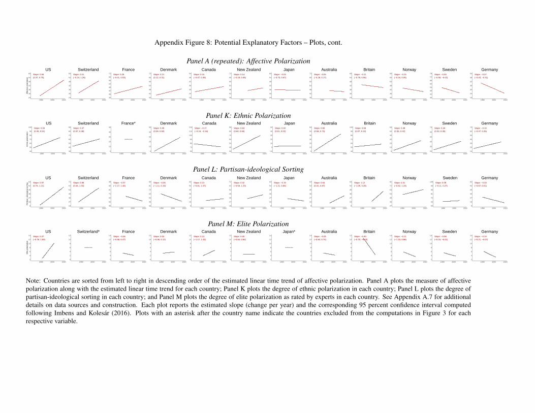
Appendix Figure 8: Potential Explanatory Factors – Plots, cont.
Panel A (repeated): Affective Polarization
Slope: 0.56
(0.37, 0.75)
24
30
36
42
48
54
60
1980 2000 2020
Affe
ctiv
e po
lariz
atio
n
USSlope: 0.51
(−0.24, 1.26)
24
30
36
42
48
54
60
1980 2000 2020
SwitzerlandSlope: 0.26
(−0.01, 0.53)
30
36
42
48
54
60
66
72
1980 2000 2020
FranceSlope: 0.21
(0.12, 0.31)
36
42
48
54
60
66
72
1980 2000 2020
DenmarkSlope: 0.15
(−0.07, 0.38)
18
24
30
36
42
48
54
1980 2000 2020
CanadaSlope: 0.14
(−0.18, 0.46)
36
42
48
54
60
66
72
1980 2000 2020
New ZealandSlope: −0.03
(−0.73, 0.67)
24
30
36
42
48
54
60
1980 2000 2020
JapanSlope: −0.05
(−0.28, 0.17)
36
42
48
54
60
66
72
1980 2000 2020
AustraliaSlope: −0.11
(−0.78, 0.56)
24
30
36
42
48
54
60
1980 2000 2020
BritainSlope: −0.15
(−0.34, 0.05)
30
36
42
48
54
60
66
1980 2000 2020
NorwaySlope: −0.30
(−0.58, −0.02)
36
42
48
54
60
66
72
78
1980 2000 2020
SwedenSlope: −0.37
(−0.43, −0.31)
18
24
30
36
42
48
54
1980 2000 2020
Germany
Panel K: Ethnic PolarizationSlope: 0.50
(0.49, 0.51)
40
50
60
70
80
90
100
1980 2000 2020
Eth
nic
pola
rizat
ion
USSlope: 0.37
(0.37, 0.38)
30
40
50
60
70
80
90
1980 2000 2020
Switzerland
Insufficient data
0
10
20
30
40
50
1980 2000 2020
France*Slope: 0.45
(0.39, 0.50)
0
10
20
30
40
50
1980 2000 2020
DenmarkSlope: −0.17
(−0.18, −0.16)
60
70
80
90
100
110
120
1980 2000 2020
CanadaSlope: 0.63
(0.60, 0.65)
30
40
50
60
70
80
90
1980 2000 2020
New ZealandSlope: 0.02
(0.01, 0.02)
−10
0
10
20
30
40
50
1980 2000 2020
JapanSlope: 0.65
(0.58, 0.73)
0
10
20
30
40
50
60
1980 2000 2020
AustraliaSlope: 0.08
(0.07, 0.10)
40
50
60
70
80
90
100
1980 2000 2020
BritainSlope: 0.38
(0.35, 0.42)
0
10
20
30
40
50
60
1980 2000 2020
NorwaySlope: 0.34
(0.33, 0.35)
20
30
40
50
60
70
1980 2000 2020
SwedenSlope: −0.10
(−0.47, 0.26)
10
20
30
40
50
60
70
1980 2000 2020
Germany
Panel L: Partisan-ideological Sorting
Slope: 0.97
(0.74, 1.21)
9
18
27
36
45
54
63
1980 2000 2020
Par
tisan
−id
eolo
gica
l sor
ting
USSlope: 0.88
(0.44, 1.33)
18
27
36
45
54
63
72
1980 2000 2020
SwitzerlandSlope: −0.37
(−2.17, 1.44)
45
54
63
72
81
90
99
1980 2000 2020
FranceSlope: −0.46
(−1.11, 0.19)
36
45
54
63
72
81
90
1980 2000 2020
DenmarkSlope: 0.13
(−0.81, 1.07)
9
18
27
36
45
54
63
1980 2000 2020
CanadaSlope: 0.32
(−0.59, 1.23)
18
27
36
45
54
63
72
1980 2000 2020
New ZealandSlope: −0.19
(−1.21, 0.84)
9
18
27
36
45
54
63
1980 2000 2020
JapanSlope: 0.64
(0.41, 0.87)
9
18
27
36
45
54
63
1980 2000 2020
AustraliaSlope: 1.12
(−1.05, 3.28)
9
18
27
36
45
54
63
1980 2000 2020
BritainSlope: 0.31
(−0.62, 1.24)
27
36
45
54
63
72
81
1980 2000 2020
NorwaySlope: 0.08
(−0.11, 0.27)
54
63
72
81
90
99
108
1980 2000 2020
SwedenSlope: −0.33
(−0.67, 0.01)
9
18
27
36
45
54
63
1980 2000 2020
Germany
Panel M: Elite PolarizationSlope: 0.37
(−0.76, 1.50)
2
4
6
8
10
12
14
1980 2000 2020
Elit
e po
lariz
atio
n
US
Insufficient data
0
2
4
6
8
10
12
1980 2000 2020
Switzerland*Slope: −0.06
(−0.58, 0.47)
2
4
6
8
10
12
14
1980 2000 2020
FranceSlope: 0.03
(−0.06, 0.12)
0
2
4
6
8
10
12
1980 2000 2020
DenmarkSlope: 0.13
(−1.17, 1.43)
0
2
4
6
8
10
12
1980 2000 2020
CanadaSlope: 0.00
(−0.84, 0.84)
0
2
4
6
8
10
12
1980 2000 2020
New Zealand
Insufficient data
2
4
6
8
10
12
14
1980 2000 2020
Japan*Slope: −0.05
(−0.84, 0.74)
2
4
6
8
10
12
14
1980 2000 2020
AustraliaSlope: −0.40
(−0.70, −0.10)
0
2
4
6
8
10
12
1980 2000 2020
BritainSlope: −0.11
(−1.10, 0.88)
2
4
6
8
10
12
14
1980 2000 2020
NorwaySlope: −0.08
(−0.15, −0.01)
2
4
6
8
10
12
14
1980 2000 2020
SwedenSlope: −0.14
(−0.21, −0.07)
2
4
6
8
10
12
14
1980 2000 2020
Germany
Note: Countries are sorted from left to right in descending order of the estimated linear time trend of affective polarization. Panel A plots the measure of affectivepolarization along with the estimated linear time trend for each country; Panel K plots the degree of ethnic polarization in each country; Panel L plots the degree ofpartisan-ideological sorting in each country; and Panel M plots the degree of elite polarization as rated by experts in each country. See Appendix A.7 for additionaldetails on data sources and construction. Each plot reports the estimated slope (change per year) and the corresponding 95 percent confidence interval computedfollowing Imbens and Kolesar (2016). Plots with an asterisk after the country name indicate the countries excluded from the computations in Figure 3 for eachrespective variable.

Appendix Figure 9: Trends in Additional Potential Explanatory Variables
rank cor: −0.294rank p−value: 0.355
CANDNK
FRA
NZL
CHEUSA
AUSGBR
DEU
JPN
NOR
SWE
0.0
0.5
3.50 3.75 4.00 4.25Internet penetration trend
Affe
ctiv
e po
lariz
atio
n tr
end
rank cor: 0.255rank p−value: 0.451
CANDNK
FRA
CHEUSA
AUSGBR
DEU
JPN
NOR
SWE
0.0
0.5
0.3 0.6 0.9Priv. 24−hr TV news (share) trend
Affe
ctiv
e po
lariz
atio
n tr
end
rank cor: 0.545rank p−value: 0.088
CANDNK
NZL
CHEUSA
AUSGBR
DEU
JPN
NOR
SWE
0.0
0.5
−0.25 0.00 0.25 0.50Ethnic fractionalization trend
Affe
ctiv
e po
lariz
atio
n tr
end
rank cor: 0.318rank p−value: 0.342
CANDNK
NZL
CHEUSA
AUSGBR
DEU
JPN
NOR
SWE
0.0
0.5
0.00 0.25 0.50Ethnic polarization trend
Affe
ctiv
e po
lariz
atio
n tr
end
Note: Each plot is a scatterplot. The y-axis variable is the estimated linear trend in affective polarization reported in Figure 1. The x-axis variable
is the estimated linear trend in the explanatory variable reported in Appendix Figure 8, subject to the sample restrictions detailed there. The rank
correlation is the Spearman rank correlation between the y-axis and x-axis variables. The rank p-value is for a test of the hypothesis that the rank of
the linear slope of affective polarization is independent of the rank of the linear slope of the explanatory variable. The test statistic is the Spearman
rank correlation and the p-value is computed via permutation, except in the case of exact ties in the ranks when we use the AS89 approximation
(Best and Roberts 1975). The best fit line is the line of best least-squares fit to the scatterplot and is plotted in black. See Appendix Figure 8 for
plots of the available data for each country and explanatory variable and Appendix A.7 for additional details on data sources and construction.
33

Appendix Table 1: Pairwise Correlations of Trends in Explanatory Variables
Economic and Media-Related Demographic and Political
Inequality (Gini) 1.00 -0.19 0.68 -0.53 0.43 0.12 0.22 -0.19Trade share of GDP -0.19 1.00 -0.01 -0.03 -0.08 -0.05 -0.55 0.01Share getting news online 0.68 -0.01 1.00 -0.62 0.75 0.24 0.14 -0.07Priv. 24-hr TV news (count) -0.53 -0.03 -0.62 1.00 -0.75 0.39 -0.12 0.58
Foreign-born share 0.43 -0.08 0.75 -0.75 1.00 0.05 0.52 -0.30Non-white share 0.12 -0.05 0.24 0.39 0.05 1.00 0.33 0.87Partisan-ideological sorting 0.22 -0.55 0.14 -0.12 0.52 0.33 1.00 -0.03Elite polarization -0.19 0.01 -0.07 0.58 -0.30 0.87 -0.03 1.00
Note: Table shows the pairwise Spearman rank correlations of the linear trends in the explanatory variables plotted in Figure 3. Pairwise complete observations areused to compute each correlation. The order of columns matches the order of rows.
34

A.4 List of Available Surveys for 1973 OECD Members
Appendix Figure 10: Surveys with Party Affect Questions
Turkey
Spain
Portugal
Netherlands
Luxembourg
Italy
Ireland
Iceland
Greece
Finland
Belgium
Austria
US
UK (Britain)
Switzerland
Sweden
Norway
New Zealand
Japan
Germany
France
Denmark
Canada
Australia
1970 1980 1990 2000 2010 2020Year
Cou
ntry
Note: For each member of the OECD as of 1973, the plot indicates election studies with party affect questions that weare aware of. The bolded names indicate the countries in our sample and the black dots indicate survey years in oursample. The non-bolded names indicate countries not in our sample and the gray dots indicate survey years not in oursample. The grey, dotted vertical line indicates 1985.
35

Appendix Table 2: Sources for Surveys with Party Affect Questions
Country In Sample Sources
Australia X https://australianelectionstudy.org/
Austria CSES
Belgium https://soc.kuleuven.be/ceso/ispo/projects/; https://easy.dans.knaw.nl/ui/home
Canada X https://www.queensu.ca/cora/our-data/data-holdings; ICPSR 7009; ICPSR 7379
Denmark X http://cssr.surveybank.aau.dk/webview/
Finland https://services.fsd.uta.fi/catalogue/index; CSES
France X ICPSR 7372; ICPSR 6583; CSES
(West) Germany X https://www.gesis.org/
Greece CSES; http://www.elnes.gr/studies; https://u.osu.edu/cnep/surveys/surveys-through-2012/
Iceland https://fel.hi.is
Ireland CSES; https://www.ucd.ie/issda/data/irishnationalelectionstudy/
Italy http://www.itanes.org/dati/
Japan X ICPSR 7294; ICPSR 4682; CSES; https://u.osu.edu/cnep/
Luxembourg
Netherlands ICPSR 28221; https://www.nkodata.nl/study units/view/11; CSES
New Zealand X http://www.nzes.org/
Norway X https://www.nsd.no/nsddata/serier/norske valgundersokelser eng.html
Portugal https://dados.rcaap.pt/handle/10400.20/2080
Spain CSES
Sweden X https://www.gu.se/valforskningsprogrammet
Switzerland X https://forscenter.ch/projects/selects/
Turkey CSES
UK (Britain) X https://www.britishelectionstudy.com/
US X https://electionstudies.org/
Note: For each member of the OECD as of 1973, the table lists sources for accessing the election studies studies described in Appendix Figure 10.
36
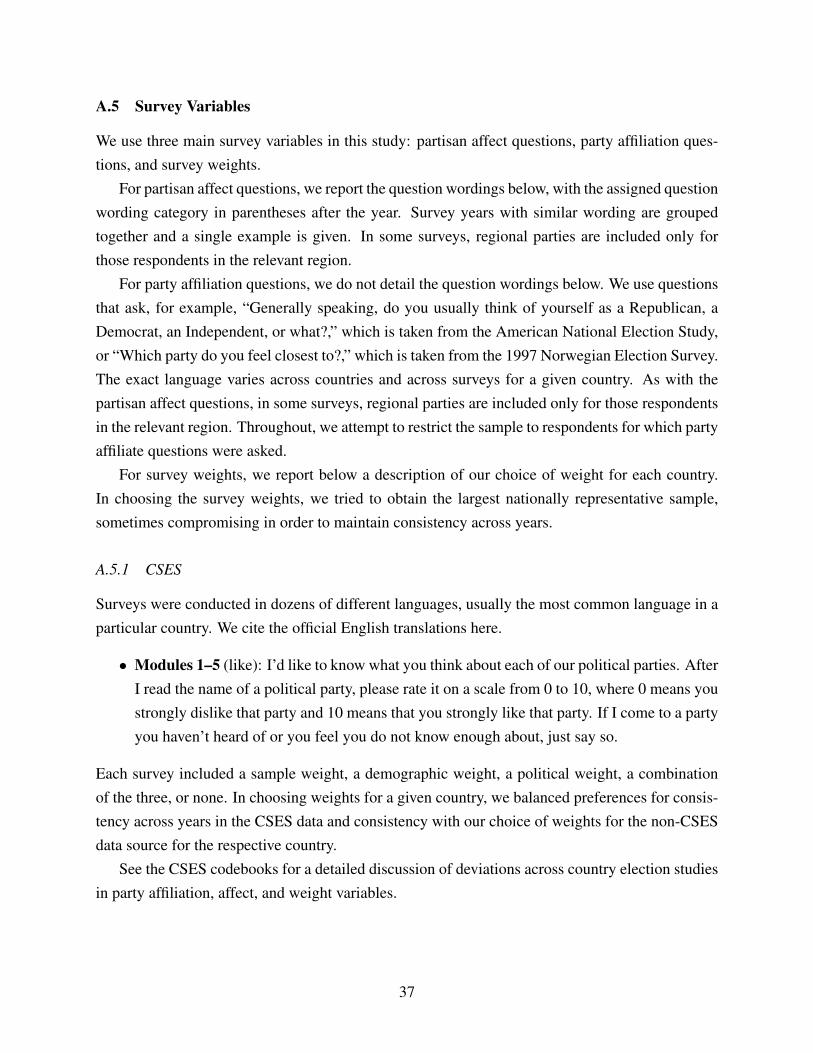
A.5 Survey Variables
We use three main survey variables in this study: partisan affect questions, party affiliation ques-tions, and survey weights.
For partisan affect questions, we report the question wordings below, with the assigned questionwording category in parentheses after the year. Survey years with similar wording are groupedtogether and a single example is given. In some surveys, regional parties are included only forthose respondents in the relevant region.
For party affiliation questions, we do not detail the question wordings below. We use questionsthat ask, for example, “Generally speaking, do you usually think of yourself as a Republican, aDemocrat, an Independent, or what?,” which is taken from the American National Election Study,or “Which party do you feel closest to?,” which is taken from the 1997 Norwegian Election Survey.The exact language varies across countries and across surveys for a given country. As with thepartisan affect questions, in some surveys, regional parties are included only for those respondentsin the relevant region. Throughout, we attempt to restrict the sample to respondents for which partyaffiliate questions were asked.
For survey weights, we report below a description of our choice of weight for each country.In choosing the survey weights, we tried to obtain the largest nationally representative sample,sometimes compromising in order to maintain consistency across years.
A.5.1 CSES
Surveys were conducted in dozens of different languages, usually the most common language in aparticular country. We cite the official English translations here.
• Modules 1–5 (like): I’d like to know what you think about each of our political parties. AfterI read the name of a political party, please rate it on a scale from 0 to 10, where 0 means youstrongly dislike that party and 10 means that you strongly like that party. If I come to a partyyou haven’t heard of or you feel you do not know enough about, just say so.
Each survey included a sample weight, a demographic weight, a political weight, a combinationof the three, or none. In choosing weights for a given country, we balanced preferences for consis-tency across years in the CSES data and consistency with our choice of weights for the non-CSESdata source for the respective country.
See the CSES codebooks for a detailed discussion of deviations across country election studiesin party affiliation, affect, and weight variables.
37

A.5.2 Australia
We exclude online survey respondents from 2001. Surveys were conducted in English. Partisanaffect questions are as follows.
• 1993 (favourable): Finally in this section, we would like to know your feelings about thepolitical parties. Please show how you feel about them by circling a number from 0 to 10.10 is the highest rating, if you feel very favourable about a party, and 0 is the lowest rating,for parties you feel very unfavourable about. If you are neutral about a particular party ordon’t know much about them, you should give them a rating of 5.
• 1996/1998/2001/2004/2007/2010/2013/2016/2019 (like): Finally in this section, we wouldlike to know what you think about each of our political parties. Please rate each party ona scale from 0 to 10, where 0 means you strongly dislike that party and 10 means that youstrongly like that party. If you are neutral about a particular party or don’t know much aboutthem, you should give them a rating of 5.
For the 1993, 2010, and 2013 surveys, there is a single choice of weight variable. For the 2016and the 2019 surveys, there are multiple weight options, and we choose the weight variables thataccount for data from all sampling approaches. All other surveys are self-weighting.
A.5.3 Britain
Surveys were conducted in English. Partisan affect questions are as follows.
• 1979 (like): Let’s say that you gave each of the parties a mark out of ten points—a markaccording to how much or how little you like it. You can give each party any mark from 0out of 10 for the least like, to 10 out of 10 for the most liked. What mark out of 10 wouldyou give the [Insert Party Name]?
• 1987/1992 (favour-against): Please choose a phrase from this card to say how you feel aboutthe Party? (Strongly in favor, In favor, Neither in favour/nor against, Against, Stronglyagainst, DK/Can’t say)
• 1997/2001/2005/2010/2015 (like): I’m now going to ask a few questions about politicalparties. On a scale that runs from 0 to 10, where 0 means strongly dislike and 10 meansstrongly like, how do you feel about the Party?
The 1979 survey is self-weighting. For 1987 and 1992, there is a single weight variable thatweights respondents by region. There are multiple weight variables for all other surveys, and weattempt to select a weight variable for each survey that is similar to the weight variables used inearlier surveys.
38
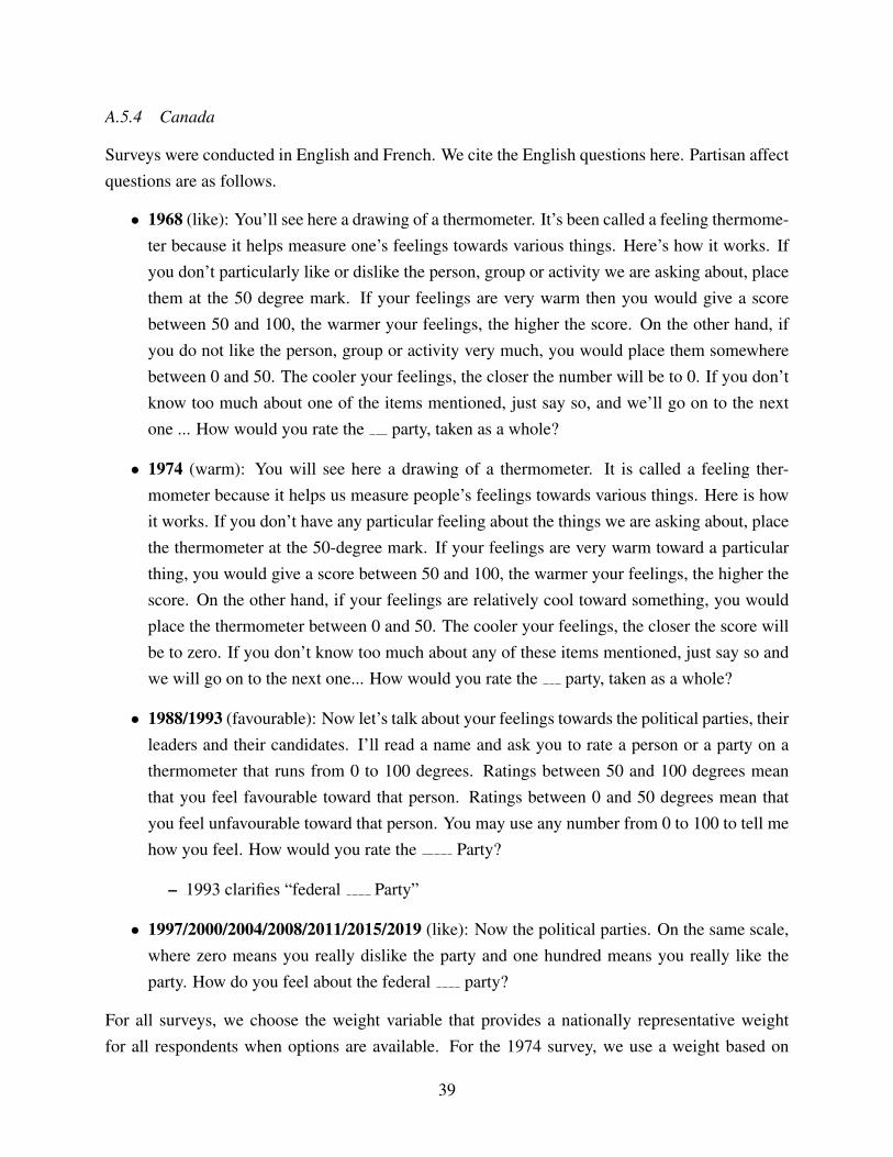
A.5.4 Canada
Surveys were conducted in English and French. We cite the English questions here. Partisan affectquestions are as follows.
• 1968 (like): You’ll see here a drawing of a thermometer. It’s been called a feeling thermome-ter because it helps measure one’s feelings towards various things. Here’s how it works. Ifyou don’t particularly like or dislike the person, group or activity we are asking about, placethem at the 50 degree mark. If your feelings are very warm then you would give a scorebetween 50 and 100, the warmer your feelings, the higher the score. On the other hand, ifyou do not like the person, group or activity very much, you would place them somewherebetween 0 and 50. The cooler your feelings, the closer the number will be to 0. If you don’tknow too much about one of the items mentioned, just say so, and we’ll go on to the nextone ... How would you rate the party, taken as a whole?
• 1974 (warm): You will see here a drawing of a thermometer. It is called a feeling ther-mometer because it helps us measure people’s feelings towards various things. Here is howit works. If you don’t have any particular feeling about the things we are asking about, placethe thermometer at the 50-degree mark. If your feelings are very warm toward a particularthing, you would give a score between 50 and 100, the warmer your feelings, the higher thescore. On the other hand, if your feelings are relatively cool toward something, you wouldplace the thermometer between 0 and 50. The cooler your feelings, the closer the score willbe to zero. If you don’t know too much about any of these items mentioned, just say so andwe will go on to the next one... How would you rate the party, taken as a whole?
• 1988/1993 (favourable): Now let’s talk about your feelings towards the political parties, theirleaders and their candidates. I’ll read a name and ask you to rate a person or a party on athermometer that runs from 0 to 100 degrees. Ratings between 50 and 100 degrees meanthat you feel favourable toward that person. Ratings between 0 and 50 degrees mean thatyou feel unfavourable toward that person. You may use any number from 0 to 100 to tell mehow you feel. How would you rate the Party?
– 1993 clarifies “federal Party”
• 1997/2000/2004/2008/2011/2015/2019 (like): Now the political parties. On the same scale,where zero means you really dislike the party and one hundred means you really like theparty. How do you feel about the federal party?
For all surveys, we choose the weight variable that provides a nationally representative weightfor all respondents when options are available. For the 1974 survey, we use a weight based on
39
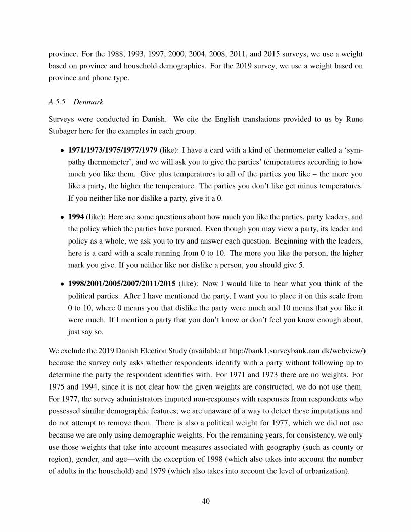
province. For the 1988, 1993, 1997, 2000, 2004, 2008, 2011, and 2015 surveys, we use a weightbased on province and household demographics. For the 2019 survey, we use a weight based onprovince and phone type.
A.5.5 Denmark
Surveys were conducted in Danish. We cite the English translations provided to us by RuneStubager here for the examples in each group.
• 1971/1973/1975/1977/1979 (like): I have a card with a kind of thermometer called a ‘sym-pathy thermometer’, and we will ask you to give the parties’ temperatures according to howmuch you like them. Give plus temperatures to all of the parties you like – the more youlike a party, the higher the temperature. The parties you don’t like get minus temperatures.If you neither like nor dislike a party, give it a 0.
• 1994 (like): Here are some questions about how much you like the parties, party leaders, andthe policy which the parties have pursued. Even though you may view a party, its leader andpolicy as a whole, we ask you to try and answer each question. Beginning with the leaders,here is a card with a scale running from 0 to 10. The more you like the person, the highermark you give. If you neither like nor dislike a person, you should give 5.
• 1998/2001/2005/2007/2011/2015 (like): Now I would like to hear what you think of thepolitical parties. After I have mentioned the party, I want you to place it on this scale from0 to 10, where 0 means you that dislike the party were much and 10 means that you like itwere much. If I mention a party that you don’t know or don’t feel you know enough about,just say so.
We exclude the 2019 Danish Election Study (available at http://bank1.surveybank.aau.dk/webview/)because the survey only asks whether respondents identify with a party without following up todetermine the party the respondent identifies with. For 1971 and 1973 there are no weights. For1975 and 1994, since it is not clear how the given weights are constructed, we do not use them.For 1977, the survey administrators imputed non-responses with responses from respondents whopossessed similar demographic features; we are unaware of a way to detect these imputations anddo not attempt to remove them. There is also a political weight for 1977, which we did not usebecause we are only using demographic weights. For the remaining years, for consistency, we onlyuse those weights that take into account measures associated with geography (such as county orregion), gender, and age—with the exception of 1998 (which also takes into account the numberof adults in the household) and 1979 (which also takes into account the level of urbanization).
40

A.5.6 France
Surveys were conducted in French. We cite the provided English translation for the 1967 survey,while we cite our own translation for the 1988 survey.
• 1967 (close-negative feelings): There are groups and individuals who influence governmentand public opinion. We would like to know your feelings in respect to them. Would you puta figure between 0 and 100 by these persons or groups according to the feelings which youhave for them. 100 = close feelings. 50 = neither for nor against. 0 = negative feelings.
– In the raw data provided, responses between 0 and 2 were coded as 2 and responses be-tween 97 and 100 were coded as 97. We recode these values to 0 and 100 respectively.
– We grouped the parties “UNR (nothing more precise)” and “UNR - leftist; Gaullists ofthe left; UDT”, which had 353 and 4 affiliates respectively, together.
• 1988 (sympathy): I would now like to know your personal feeling on political parties andthe main candidates for the private election. Using this scale, do you want to put a scorefrom 0 to 100 to the people or groups that I will name you in depending on your sympathyfor them. -100 means you have a lot of sympathy - 0 means you don’t like it at all - 50 meansyou have neither sympathy nor antipathy or that you don’t know much of them. What gradewould you give to:
• 2002, 2007, 2012, 2017: We use data from the CSES. See the CSES question wording.
There is a single choice of weight variable for 1967. No weight variables were provided for 1988.
A.5.7 (West) Germany
We drop observations in some months of 1982, 1987 and 1988 where multiple versions of thequestionnaire were used (see variable v79 in the data outlining these observations). We drop du-plicate respondents. We restrict attention to West Germany (see variable V4a), except for the years1996–1998 when the surveys were not separately conducted between the two regions. In Ap-pendix Figure 11 below, we compare trends in East versus West Germany, excluding 1996–1998when these regions are not distinguished.
41

Appendix Figure 11: Trends in Affective Polarization—East vs. West Germany
Slope: −0.22(−0.31,−0.12)
Slope: −0.37(−0.43,−0.31)
15
20
25
30
35
40
45
50
55
60
1980 2000 2020
Affe
ctiv
e po
lariz
atio
n
Type
East: −5 to 5 (think highly)
West: −5 to 5 (think highly)
Germany
Note: The plot shows estimates of affective polarization Π as defined in Section 2 across two different seriesconstructed from the Politbaroameter survey conducted in the Germany. One point represents one survey.The red line with triangle markers uses data from West Germany. The black line with the circle markers usesdata from East Germany. Each line is a fitted bivariate linear regression line with affective polarization asthe dependent variable and survey year as the independent variable. The estimated slopes (change per year)and the corresponding 95 percent confidence intervals, computed following Imbens and Kolesar (2016), arealso reported. We exclude data from 1996–1998 for both series because the surveys do not distinguish Eastand West Germany in these years.
Surveys were conducted in German. We translate the question ourselves. Partisan affect questionsare as follows.
• All years (think highly): Imagine a thermometer that goes from +5 to -5 with a 0 point inbetween. With this thermometer, tell me what you think of the individual parties. +5 meansthat you think highly of the party. -5 means you don’t think anything of it at all. With thevalues in between, you can give your opinion in stages.
There is a single choice of weight variable for all years.
A.5.8 Japan
Surveys were conducted in Japanese. We cite the official English translation here. Partisan affectquestions are as follows.
• 1967 (like): Now I am going to ask you whether you like or dislike political parties. Howmuch do you like ?
42

– Like = 1, Like a Little = 2, Depends = 3, Dislike a Little = 4, Dislike = 5
• 1976 (like): People have all kinds of feelings toward the people and groups which are influ-ential in politics. In answering the following questions, if you don’t like or dislike a personor group would you indicate this by giving them a rating of 50 degrees? If you like the per-son or group would you give them a rating between 50 and 100 degrees, and if you dislikethem a rating between 0 and 50 degrees?
• 1996, 2004, 2007, 2013: We use data from the CSES. See the CSES question wording.
There is either a single choice of weight or no weight in 1967 and 1976. For weight choices inlatter years, see CSES.
A.5.9 New Zealand
Surveys were conducted in English and Maori. We cite the English questions here. Partisan affectquestions are as follows.
• 1990/1993 (support-oppose): Regardless of what their chances were in winning your partic-ular electorate, or even winning any seats at all, how do you feel about these political parties?(Strongly Support = 1, Support = 2, Neutral = 3, Oppose = 4, Strongly Oppose = 5 )
• 1996/1999/2002/2005/2008/2011/2014/2017 (like): We would like to know what you thinkabout each of these political parties. Please rate each party on a scale from 0 to 10, where 0means you strongly dislike that party and 10 means that you strongly like that party. If youhaven’t heard about that party or don’t know enough about it, please circle ‘99’ under ‘don’tknow’. How do you feel about: [Insert Party Name]
For all surveys, we use weights associated with validated voters only for consistency across sur-veys. Weights for non-validated voters are not reported in the surveys between 2008 and 2017.
A.5.10 Norway
Surveys were conducted in Norwegian. We cite the official English translation here. Partisan affectquestions are as follows.
• 1981/1985/1989/1993 (like): We want to know how much or little you like the differentparties. On this card is a scale that we call “sympathy thermometer.” At 50-degrees-lineposition the parties that you neither like or dislike. A party that you like to have a locationfrom 50 to 100 degrees. The better you like the party, the higher position. However, if it is aparty you do not like, it should be placed between 0 and 50 degrees, with 0 as the expressionof at least sympathy.
43

• 1997/2001/2005/2009/2013/2017 (like): After I read the name of a political party, pleaserate it on a scale from 0 to 10, where 0 means you strongly dislike that party and 10 meansthat you strongly like that party.
All surveys except 2013 and 2017 are self-weighting. For the 2013 survey, we use the weightvariable that includes mail-in respondents. For the 2017 survey, we use the post-stratified weightvariable based on gender, education, and age.
A.5.11 Sweden
Surveys were conducted in Swedish. We cite the official English translation here. Partisan affectquestions are as follows.
• All Years (like): On this card there is a kind of scale. I would like you to use it in order tostate how much you like or dislike the parties. If you like a party, use the “plus” figures. Thebetter you like a party the higher the “plus” figure. For parties you dislike, use the “minus”figures. The more you dislike a party, the higher the “minus” figure. The zero point on thescale indicates that you neither like nor dislike a party. Where would you like to place the
? (Ranges from -5 to 5.)
All surveys are self-weighting.
A.5.12 Switzerland
Surveys were conducted in German, French and Italian. We translate the questions ourselves.Partisan affect questions are as follows.
• 1975 (like): Here is a scale we call a favorability thermometer. Please give a score between0 and 100 indicating how much you like the following groups and organizations. 100 meansthat you like them very much, 0 means that you do not like them at all. If you don’t partic-ularly like or dislike them... give a score of 50. What score would you give to [Insert PartyName]?
• 1995/1999 (sympathy): Now I would like to know what you think of our political parties.When I read the name of a political party to you, please indicate where you place it on a scalefrom 0 to 10, with 0 meaning “no sympathy at all”, and 10 meaning “a lot of sympathy”.
• 2003: We use data from the CSES. See the CSES question wording.
• 2007 (like): We would now like to know what you think of some of the political parties.Please place the on a scale from 0 to 10. 0 means that you do not like this party atall. 10 means you like this party very much.
44
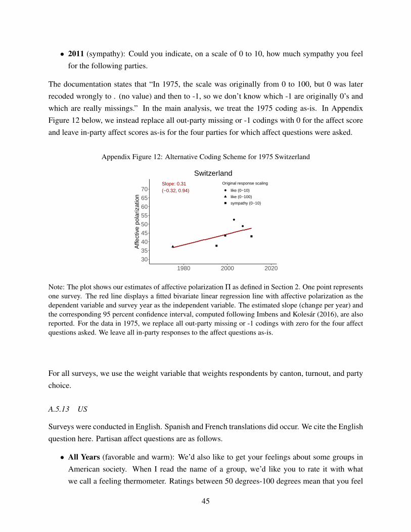
• 2011 (sympathy): Could you indicate, on a scale of 0 to 10, how much sympathy you feelfor the following parties.
The documentation states that “In 1975, the scale was originally from 0 to 100, but 0 was laterrecoded wrongly to . (no value) and then to -1, so we don’t know which -1 are originally 0’s andwhich are really missings.” In the main analysis, we treat the 1975 coding as-is. In AppendixFigure 12 below, we instead replace all out-party missing or -1 codings with 0 for the affect scoreand leave in-party affect scores as-is for the four parties for which affect questions were asked.
Appendix Figure 12: Alternative Coding Scheme for 1975 Switzerland
Slope: 0.31(−0.32, 0.94)
30
35
40
45
50
55
60
65
70
1980 2000 2020
Affe
ctiv
e po
lariz
atio
n
Original response scaling
like (0−10)
like (0−100)
sympathy (0−10)
Switzerland
Note: The plot shows our estimates of affective polarization Π as defined in Section 2. One point representsone survey. The red line displays a fitted bivariate linear regression line with affective polarization as thedependent variable and survey year as the independent variable. The estimated slope (change per year) andthe corresponding 95 percent confidence interval, computed following Imbens and Kolesar (2016), are alsoreported. For the data in 1975, we replace all out-party missing or -1 codings with zero for the four affectquestions asked. We leave all in-party responses to the affect questions as-is.
For all surveys, we use the weight variable that weights respondents by canton, turnout, and partychoice.
A.5.13 US
Surveys were conducted in English. Spanish and French translations did occur. We cite the Englishquestion here. Partisan affect questions are as follows.
• All Years (favorable and warm): We’d also like to get your feelings about some groups inAmerican society. When I read the name of a group, we’d like you to rate it with whatwe call a feeling thermometer. Ratings between 50 degrees-100 degrees mean that you feel
45
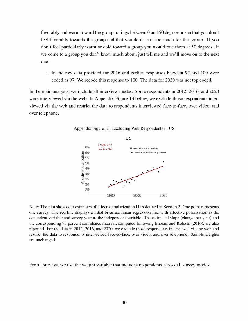
favorably and warm toward the group; ratings between 0 and 50 degrees mean that you don’tfeel favorably towards the group and that you don’t care too much for that group. If youdon’t feel particularly warm or cold toward a group you would rate them at 50 degrees. Ifwe come to a group you don’t know much about, just tell me and we’ll move on to the nextone.
– In the raw data provided for 2016 and earlier, responses between 97 and 100 werecoded as 97. We recode this response to 100. The data for 2020 was not top coded.
In the main analysis, we include all interview modes. Some respondents in 2012, 2016, and 2020were interviewed via the web. In Appendix Figure 13 below, we exclude those respondents inter-viewed via the web and restrict the data to respondents interviewed face-to-face, over video, andover telephone.
Appendix Figure 13: Excluding Web Respondents in US
Slope: 0.47(0.32, 0.62)
25
30
35
40
45
50
55
60
65
1980 2000 2020
Affe
ctiv
e po
lariz
atio
n
Original response scaling
favorable and warm (0−100)
US
Note: The plot shows our estimates of affective polarization Π as defined in Section 2. One point representsone survey. The red line displays a fitted bivariate linear regression line with affective polarization as thedependent variable and survey year as the independent variable. The estimated slope (change per year) andthe corresponding 95 percent confidence interval, computed following Imbens and Kolesar (2016), are alsoreported. For the data in 2012, 2016, and 2020, we exclude those respondents interviewed via the web andrestrict the data to respondents interviewed face-to-face, over video, and over telephone. Sample weightsare unchanged.
For all surveys, we use the weight variable that includes respondents across all survey modes.
46
A.6 Election Study References and Disclaimers
A.6.1 CSES
Data comes from the Comparative Study of Electoral Systems (CSES) (www.cses.org). These ma-terials are based on work supported by the American National Science Foundation (www.nsf.gov)under grant numbers SES-0817701, SES-1154687, SES-1420973, and SES-1760058, the GESIS- Leibniz Institute for the Social Sciences, the University of Michigan, in-kind support of partic-ipating election studies, the many organizations that sponsor planning meetings and conferences,and the numerous organizations that fund national election studies by CSES collaborators. Anyopinions, findings, and conclusions, or recommendations expressed in these materials are those ofthe author(s) and do not necessarily reflect the views of the funding organizations.
The Comparative Study of Electoral Systems (www.cses.org). CSES Integrated ModuleDataset Phase 3 Release [dataset and documentation]. December 8, 2020 version.doi:10.7804/cses.imd.2020-12-08.
The Comparative Study of Electoral Systems (www.cses.org). CSES Module 5 Sec-ond Advance Release [dataset and documentation]. May 14, 2020 version.doi:10.7804/cses.module5.2020-05-14.
A.6.2 Australia
Data comes from the Australian Election Study15 (https://australianelectionstudy.org/). Those whocarried out the original analysis and collection of the data bear no responsibility for the furtheranalysis or interpretation of it.
Jones, Roger; McAllister, Ian; Denemark, David; Gow, David, 2017, “Australian Election Study,1993”. doi:10.4225/87/ZZ3NOB, ADA Dataverse, V1, UNF:6:3C/DZ94Ci0V2mfL02PVpXw==
Jones, Roger; McAllister, Ian; Gow, David, 2017, “Australian Election Study, 1996” doi:10.4225/87/NSDHWM, ADA Dataverse, V1, UNF:6:V05mNiOGYLZnBaihME2SIA==
Bean, Clive; Gow, David; McAllister, Ian, 2017, “Australian Election Study, 1998” doi:10.4225/87/FFBWUU, ADA Dataverse, V2, UNF:6:pmAXB4lfnfvlseqWTWKOkg==
Bean, Clive; Gow, David; McAllister, Ian, 2017, “Australian Election Study, 2001” doi:10.4225/87/CALXMK, ADA Dataverse, V1, UNF:6:8dudxHV83HO/5+itv3DNjA==
Bean, Clive; McAllister, Ian; Gibson, Rachel; Gow, David, 2017, “Australian Election Study,2004” doi:10.4225/87/G9ITIO, ADA Dataverse, V1, UNF:6:Qer+KzJrJC+zlC3Gm6qDmw==
15Hosted at the Australian Data Archive (https://dataverse.ada.edu.au/).
47

Bean, Clive; McAllister, Ian; Gow, David, 2017, “Australian Election Study, 2007” doi:10.4225/87/ZBUOW0, ADA Dataverse, V1, UNF:6:D7a6fhN+szVMSQF9xIh5+A==
McAllister, Ian; Bean, Clive; Gibson, Rachel Kay; Pietsch, Juliet, 2017, “Australian ElectionStudy, 2010” doi:10.4225/87/CYJNSM, ADA Dataverse, V2, UNF:6:3iyzr2dBihOrVkbafFkRZA==
Bean, Clive; McAllister, Ian; Pietsch, Juliet; Gibson, Rachel Kay, 2017, “Australian ElectionStudy, 2013” doi:10.4225/87/WDBBAS, ADA Dataverse, V3, UNF:6:6gMySFLvbEH1ccG58om4Sg==
McAllister, Ian; Makkai, Toni; Bean, Clive; Gibson, Rachel Kay, 2017, “Australian Election Study,2016” doi:10.4225/87/7OZCZA, ADA Dataverse, V2, UNF:6:TNnUHDn0ZNSlIM94TQphWw==
McAllister, Ian; Bean, Clive; Gibson, Rachel; Makkai, Toni; Sheppard, Jill; Cameron, Sarah, 2019,“Australian Election Study, 2019” doi:10.26193/KMAMMW, ADA Dataverse, V2
A.6.3 Britain
Data comes from the British Election Study (https://www.britishelectionstudy.com/).16 We ac-knowledge that the BES and the relevant funding agencies bear no responsibility for use of thedata or for interpretations or inferences based upon such uses.
Crewe, I.M., Robertson, D.R. and Sarlvik, B., British Election Study, May 1979; Cross-SectionSurvey [computer file]. Colchester, Essex: UK Data Archive [distributor], 1981.17
Heath, A., Jowell, R. and Curtice, J.K., British General Election Study, 1983; Cross-Section Survey[computer file]. Colchester, Essex: UK Data Archive [distributor], 1983.18
Heath, A., Jowell, R. and Curtice, J.K., British General Election Study, 1987; Cross-Section Survey[computer file]. 2nd Edition. Colchester, Essex: UK Data Archive [distributor], April 1993.
Heath, A. et al., British General Election Study, 1992; Cross-Section Survey [computer file].Colchester, Essex: UK Data Archive [distributor], April 1993.19
Heath, A. et al., British General Election Study, 1997; Cross-Section Survey [computer file]. 2ndEdition. Colchester, Essex: UK Data Archive [distributor], May 1999.
Clarke, H. et al., British General Election Study, 2001; Cross-Section Survey [computer file].
16Some survey years are located at https://ukdataservice.ac.uk.
17As of November 16, 2021, the BES indicated this dataset was last updated on April 30, 2014.
18As of November 16, 2021, the BES indicated this dataset was last updated on May 5, 2014.
19As of November 11, 2021, the BES indicated this dataset was last updated on April 5, 2014.
48

Colchester, Essex: UK Data Archive [distributor], March 2003.20
Clarke, H. et al., British Election Study, 2005: Face-to-Face Survey [computer file]. Colchester,Essex: UK Data Archive [distributor], November 2006.21
Whiteley, P.F. and Sanders, D., British Election Study, 2010: Face-to-Face Survey [computer file].Colchester, Essex: UK Data Archive [distributor], August 2014.22
Fieldhouse, E., Green, J., Evans, G., Schmitt, H., van der Eijk, C., Mellon, J., Prosser, C. (2016).British Election Study, 2015: Face-to-Face Post-Election Survey. [data collection]. Version3.0. UK Data Service. SN: 7972, http://dx.doi.org/10.5255/UKDA-SN-7972-1
Fieldhouse, E., Green, J., Evans, G., Schmitt, H., van der Eijk, C., Mellon, J., Prosser, C. (2018).British Election Study, 2017: Face-to-Face Post-Election Survey [data collection]. Version1.0. http://doi .org/10.5255/UKDA-SN-8418-1
A.6.4 Canada
Data comes from the Canadian Election Study (https://www.queensu.ca/cora/our-data/data-holdings).Data from the 1968 Canadian National Election Study were made available by the Inter-
University Consortium for Political and Social Research. The data were originally collected byJohn Meisel of Queen’s University. Neither the original collector of the data nor the Consortiumbear any responsibility for the analyses or the interpretations presented here.
Data from the 1974 Canadian National Election Study were made available by the Inter-University Consortium for Political and Social Research. The data were originally collected byHarold Clarke, Jane Jenson, Lawrence Leduc and Jon Pammett. Neither the original collectors ofthe data nor the Consortium bear any responsibility for the analyses or the interpretations presentedhere.
1984 Canadian National Election Study, which was funded by the Social Sciences and Hu-manities Research Council of Canada, were made available by the (Study’s Principal Investigatorsor Archive). The data were collected by R.D. Lambert, S.D. Brown, J.E. Curtis, B.J. Kay and J.M.Wilson. The original collectors of the data and SSHRCC (and the Archive) bear no responsibilityfor the analyses and interpretations presented here.
Data from the 1988 Canadian National Election Study were funded by the Social Sciencesand Humanities Research Council of Canada (Grant #411-88-0030). The data were collected bythe Institute for Social Research, York University for Richard Johnston, Andre Blais, Henry E.
20As of November 11, 2021, the BES indicated this dataset was last updated on July 19, 2016.
21As of November 16, 2021, the BES indicated this dataset was last updated on January 14, 2015.
22As of November 11, 2021, the BES indicated this dataset was last updated on January 14, 2015.
49

Brady and Jean Crete. The investigators, SSHRC and the Institute for Social Research bear noresponsibility for the analyses and interpretations presented here.
Data from the 1993 Canadian Election Study were provided by the Institute for Social Re-search, York University. The survey was funded by the Social Sciences and Humanities ResearchCouncil of Canada (SSHRC), grant numbers 411-92-0019 and 421-92-0026, and was completedfor the 1992/93 Canadian Election Team of Richard Johnston (University of British Columbia),Andre Blais (Universite de Montreal), Henry Brady (University of California at Berkeley), Elisa-beth Gidengil (McGill University), and Neil Nevitte (University of Calgary). Neither the Institutefor Social Research, the SSHRC, nor the Canadian Election Team are responsible for the analysesand interpretations presented here.
Data from the 1997 Canadian Election Survey were provided by the Institute for Social Re-search, York University. The survey was funded by the Social Sciences and Humanities ResearchCouncil of Canada (SSHRC), grant number 412-96-0007 and was completed for the 1997 Cana-dian Election Team of Andre Blais (Universite de Montreal), Elisabeth Gidengil (McGill Univer-sity), Richard Nadeau (Universite de Montreal) and Neil Nevitte (University of Toronto). Neitherthe Institute for Social Research, the SSHRC, nor the Canadian Election Survey Team are respon-sible for the analyses and interpretations presented here.
Data from the 2000 Canadian Election Survey were provided by the Institute for Social Re-search, York University. The survey was funded by the Social Sciences and Humanities ResearchCouncil of Canada (SSHRC), and was completed for the 2000 Canadian Election Team of AndreBlais (Universite de Montreal), Elisabeth Gidengil (McGill University), Richard Nadeau (Uni-versite de Montreal) and Neil Nevitte (University of Toronto). Neither the Institute for SocialResearch, the SSHRC, nor the Canadian Election Survey Team are responsible for the analysesand interpretations presented here.
Data from the 2004 and the 2006 Canadian Election Surveys were provided by the Institutefor Social Research, York University. The surveys were funded by Elections Canada and the SocialSciences and Humanities Research Council of Canada (SSHRC), and was completed for the Cana-dian Election Team of Andre Blais (Universite de Montreal), Joanna Everitt, University of NewBrunswick, Patrick Fournier (Universite de Montreal), Elisabeth Gidengil (McGill University),and Neil Nevitte (University of Toronto). Neither the Institute for Social Research, the SSHRC,Elections Canada nor the Canadian Election Survey Team are responsible for the analyses andinterpretations presented here.
Data from the 2008 Canadian Election Surveys were provided by the Institute for SocialResearch, York University. The survey was funded by Elections Canada, and was completed forthe Canadian Election Team of Elisabeth Gidengil (McGill University), Joanna Everitt, Universityof New Brunswick, Patrick Fournier (Universite de Montreal), and Neil Nevitte (University of
50

Toronto). Neither the Institute for Social Research, Elections Canada, or the Canadian ElectionSurvey Team are responsible for the analyses and interpretations presented here.
Data from the 2011 Canadian Election Survey were provided by the Institute for Social Re-search, York University. The survey was funded by Elections Canada, and was completed for theCanadian Election Team of Patrick Fournier (Universite de Montreal), Fred Cutler (University ofBritish Columbia), Stuart Soroka (McGill University), and Dietlind Stolle (McGill University).Neither the Institute for Social Research, Elections Canada, or the Canadian Election Survey Teamare responsible for the analyses and interpretations presented here.
Data from the 2015 Canadian Election Study were provided by the Institute for Social Re-search, York University. The survey was funded by the Social Sciences and Humanities ResearchCouncil (SSHRC) and Elections Canada, and was completed for the Canadian Election StudyTeam of Patrick Fournier (Universite de Montreal), Fred Cutler (University of British Columbia),Stuart Soroka (University of Michigan), and Dietlind Stolle (McGill University). Neither the In-stitute for Social Research, SSHRC, Elections Canada, nor the Canadian Election Study Team areresponsible for the analyses and interpretations presented here.
Data from the Canadian Election Study, 2019, Phone Survey were produced and authoredby Laura B Stephenson (Western University), Allison Harell (Universite du Quebec a Montreal),Daniel Rubenson (Ryerson University), and Peter John Loewen (University of Toronto). The sur-vey was funded by Social Sciences and Humanities Research Council of Canada, and the data weredistributed by Canadian Opinion Research Archive, Queen’s University. Neither the Social Sci-ences and Humanities Research Council of Canada, the above-mentioned producers of the data, norCanadian Opinion Research Archive are responsible for the analyses and interpretations presentedhere.
Meisel, J. 1968. The 1968 Canadian Election Study [dataset]. Inter-University Consortium forPolitical and Social Research, University of Michigan, Ann Arbor MI [Producer and distrib-utor].
Clarke, H, Jenson, J, LeDuc, L and Pammett, J. 1975. The 1974 Canadian Election Study [dataset].Toronto, Ontario, Canada: Institute for Social Research [producer and distributor].
Lambert, R, Brown, S, Curtis, J, Kay, B, Wilson, J. 1986. The 1984 Canadian Election Study[dataset]. Toronto, Ontario, Canada: Institute for Social Research [producer and distributor].
Johnston, R, Blais, A, Brady, H. E. and Crete, J. 1989. The 1988 Canadian Election Study [dataset].Toronto, Ontario, Canada: Institute for Social Research [producer and distributor].
Blais, A, Brady, H, Gidengil, E, Johnston, R and Nevitte, N. 1994. The 1993 Canadian Elec-tion Study [dataset]. Toronto, Ontario, Canada: Institute for Social Research [producer anddistributor].
Blais, A, Gidengil, E, Nadeau, R and Nevitte, N. 1998. The 1997 Canadian Election Study
51

[dataset]. Toronto, Ontario, Canada: Institute for Social Research [producer and distributor].Blais, A, Gidengil, E, Nadeau, R and Nevitte, N. 2001. The 2000 Canadian Election Study
[dataset]. Toronto, Ontario, Canada: Institute for Social Research [producer and distributor].Blais, A, Everitt, J, Fournier, P, Gidengil, E and Nevitte, N. 2005. The 2004 Canadian Election
Study [dataset]. Toronto, Ontario, Canada: Institute for Social Research [producer and dis-tributor].
Gidengil, E, Everitt, J, Fournier, P and Nevitte, N. 2009. The 2008 Canadian Election Study[dataset]. Toronto, Ontario, Canada: Institute for Social Research [producer and distributor].
Fournier, P, Cutler, F, Soroka, S and Stolle, D. 2011. The 2011 Canadian Election Study [dataset].Toronto, Ontario, Canada: Institute for Social Research [producer and distributor].
Fournier, P, Cutler, F, Soroka, S and Stolle, D. 2016. Canadian Election Study, June 2015 [Canada].[Study Microdata]. Toronto, Ontario. Institute of Social Research [distributor]
Stephenson, Laura B., Allison Harell, Daniel Rubenson and Peter John Loewen. The 2019 Cana-dian Election Study – Phone Collection. [dataset]
A.6.5 Denmark
Data comes from the Danish Election Project made accessible by the Danish National Archive(https://www.sa.dk/da/forskning-rigsarkivet/benyt-surveydata/valgundersoegelsen/). We also sup-plemented codebooks from the National Archive with codebooks from Survey Bank (http://bank1.surveybank.aau.dk/webview/). Neither the Danish Election Project, the Danish National Archive,nor Survey Bank are responsible for the analysis/interpretation of the data presented here.
A.6.6 France
Data comes from the Inter-university Consortium for Political and Social Research (ICPSR)(https://www.icpsr.umich.edu/web/pages/index.html). The original collector of the data, ICPSR,and the relevant funding agency bear no responsibility for use of the data or for interpretations orinferences based upon such uses.
Converse, Philip E., Dupeux, Georges, and Pierce, Roy. French National Election Panel Study,1967-1969. Version V1. Ann Arbor, MI: Inter-university Consortium for Political and SocialResearch [distributor], 2006-03-30. https://doi.org/10.3886/ICPSR02978.v1
Pierce, Roy. French Presidential Election Survey, 1988. Version V1. Ann Arbor, MI: Inter-university Consortium for Political and Social Research [distributor], 1996-04-04.https://doi.org/10.3886/ICPSR06583.v1
52

A.6.7 (West) Germany
Data comes from the Politbarometers (https://www.gesis.org/en/elections-home/politbarometer/recent-time-series/). Neither the depositor (individual(s), institute(s) etc.) nor GESIS bear anyresponsibility for the analysis, the methods used for the analysis, or the interpretation with regardto contents of the data which is provided by GESIS.
Forschungsgruppe Wahlen, Mannheim (2020). Partial Cumulation of Politbarometers1977-2018. GESIS Data Archive, Cologne. ZA2391 Data file Version 11.0.0,https://doi.org/10.4232/1.13431.
A.6.8 Japan
Data comes from the Inter-university Consortium for Political and Social Research (ICPSR)(https://www.icpsr.umich.edu/web/pages/index.html). The original collector of the data, ICPSR,and the relevant funding agency bear no responsibility for uses of this collection or for interpreta-tions or inferences based upon such uses.
Ward, Robert E., and Kubota, Akira. Japanese National Election Study, 1967. Version V2. AnnArbor, MI: Inter-university Consortium for Political and Social Research [distributor], 2000-01-18. https://doi.org/10.3886/ICPSR07294.v2
Flanagan, Scott C., Kohei, Shinsaku, Miyake, Ichiro, Richardson, Bradley M., and Watanuki, Joji.JABISS: The Japanese Election Study, 1976. Version V1. Ann Arbor, MI: Inter-universityConsortium for Political and Social Research [distributor], 2008-02-27.https://doi.org/10.3886/ICPSR04682.v1
A.6.9 New Zealand
Data comes from the New Zealand Election Study (http://www.nzes.org/).
A.6.10 Norway
Data comes from the Norwegian Election Research Programme (https://nsd.no/nsddata/serier/norskevalgundersokelser eng.html).23
23Some of the data applied in the analysis in this publication are based on “Election Survey 1957 - 2017.” The data
are provided by Statistics Norway and Institute for Social Research, and prepared and made available by Norwegian
Centre for Research Data (NSD). Neither Statistics Norway, Institute for Social Research nor NSD are responsible
for the analysis/interpretation of the data presented here.
53
Norwegian Research Programme. The 1977 Norway Election Study. Second NSD Edition. Nor-wegian Centre for Research Data [distributer].
Norwegian Research Programme. The 1981 Norway Election Study. Third NSD Edition. Norwe-gian Centre for Research Data [distributer].
Norwegian Research Programme. The 1985 Norway Election Study. Second NSD Edition. Nor-wegian Centre for Research Data [distributer].
Norwegian Research Programme. The 1989 Norway Election Study. Second NSD Edition. Nor-wegian Centre for Research Data [distributer].
Norwegian Research Programme. The 1993 Norway Election Study. Third NSD Edition. Norwe-gian Centre for Research Data [distributer].
Norwegian Research Programme. The 1997 Norway Election Study. Fourth NSD Edition. Nor-wegian Centre for Research Data [distributer].
Norwegian Research Programme. The 2001 Norway Election Study. Third NSD Edition. Norwe-gian Centre for Research Data [distributer].
Norwegian Research Programme. The 2005 Norway Election Study. Third NSD Edition. Norwe-gian Centre for Research Data [distributer].
Norwegian Research Programme. The 2009 Norway Election Study. First NSD Edition. Norwe-gian Centre for Research Data [distributer].
Norwegian Research Programme. The 2013 Norway Election Study. First NSD Edition. Norwe-gian Centre for Research Data [distributer].
Norwegian Research Programme. The 2017 Norway Election Study. Second NSD Edition. Nor-wegian Centre for Research Data [distributer].
A.6.11 Sweden
Data comes from the Swedish National Election Studies (https://www.gu.se/en/swedish-national-election-studies). Neither SND nor the principal investigator take any responsibility for howthe data are used, nor for any interpretations of or conclusions based on it.
Soren Holmberg, Statistics Sweden. University of Gothenburg, Department of Political Science(1986). Swedish election study 1979. Swedish National Data Service. Version 1.0. https://doi.org/10.5878/002509
Soren Holmberg, Statistics Sweden. University of Gothenburg, Department of Political Science(1986). Swedish election study 1982. Swedish National Data Service. Version 1.0. https://doi.org/10.5878/002510
Soren Holmberg, Mikael Gilljam, Statistics Sweden. University of Gothenburg, Department of Po-litical Science (1991). Swedish election study 1985. Swedish National Data Service. Version
54

1.0. https://doi.org/10.5878/002511Soren Holmberg, Mikael Gilljam, Statistics Sweden. University of Gothenburg, Department of Po-
litical Science (1991). Swedish election study 1988. Swedish National Data Service. Version1.0. https://doi.org/10.5878/002512
Soren Holmberg, Mikael Gilljam, Statistics Sweden. University of Gothenburg, Department of Po-litical Science (1997). Swedish election study 1994. Swedish National Data Service. Version1.0. https://doi.org/10.5878/002514
Soren Holmberg, Statistics Sweden. University of Gothenburg, Department of Political Science(2002). Swedish election study 1998. Swedish National Data Service. Version 1.0. https://doi.org/10.5878/002515
Soren Holmberg, Henrik Ekengren Oscarsson, Statistics Sweden. University of Gothenburg, De-partment of Political Science (2006). Swedish election study 2002. Swedish National DataService. Version 1.0. https://doi.org/10.5878/002643
Soren Holmberg, Henrik Ekengren Oscarsson, Statistics Sweden. University of Gothenburg, De-partment of Political Science (2012). Swedish election study 2006. Swedish National DataService. Version 2.0. https://doi.org/10.5878/002526
Soren Holmberg, Henrik Ekengren Oscarsson. University of Gothenburg, Department of PoliticalScience (2017). Swedish election study 2010. Swedish National Data Service. Version 1.0.https://doi.org/10.5878/002905
A.6.12 Switzerland
Data comes from the Swiss Election Study (https://forscenter.ch/projects/selects/).
Selects: Swiss national election studies, cumulated file 1971-2015 [Dataset]. Version 1.0.0. Dis-tributed by FORS, Lausanne, 2017. https://doi.org/10.23662/FORS-DS-495-2.
A.6.13 US
Data comes from The American National Election Study (https://electionstudies.org/). In our mainanalysis, we use the 1948–2016 Time Series Cumulative Data File and the 2020 Time Series Study.We also use the 1996, 2004, 2008, 2012, and 2016 Time Series Studies for specific robustnesstests. The original collector of the data, ANES, and the relevant funding agency/agencies bear noresponsibility for use of the data or for interpretations or inferences based upon such uses.
The American National Election Study (https://electionstudies.org/). These materials are basedon work supported by the National Science Foundation under grant numbers SES 1444721,2014-2017, the University of Michigan, and Stanford University.
55

A.7 Data Sources for Potential Explanatory Variables
See Appendix Figure 8 for plots of the available data for each country and variable.
• Inequality (Gini): Gini coefficient from Roser and Ortiz-Ospina (2013) and Gini Index(World Bank estimate) from the World Bank (2020a). For each country, we use the dataseries that covers more years, and report in Appendix Table 3 the correlation between thetwo series for overlapping years.
• Trade Share of GDP: Trade (percent of GDP) from the World Bank (2020b). Defined tobe the the sum of exports and imports of goods and services measured as a share of grossdomestic product.
• Internet Penetration: Individuals using the internet (percent of population) from the WorldBank (2020c). Defined to be individuals (percent of population) who have used the Internet(from any location) in the last 3 months.
• Share Getting News Online: Share of respondents in the Reuters Institute Digital NewsReport 2020 survey (Newman et al. 2020) who reported getting news online (includingsocial media) in the last week. We assume the 1995 value for each country is 0.
• Priv. 24-hr TV News (Share): Share of respondents in the Reuters Institute Digital NewsReport 2020 survey (Newman et al. 2020) who reported watching the largest private 24-hour TV news network in the last week. We assume the value for each country was zero in1980, the launch year of CNN (the first 24-hr private news network).
• Priv. 24-hr TV News (Count): The number of private 24-hour TV news networks in theReuters Institute Digital News Report 2020 survey (Newman et al. 2020). We assume thevalue for each country was zero in 1980, the launch year of CNN (the first 24-hr private newsnetwork).
• Foreign-born Share: We impute the share of foreign-born population using stocks of foreign-born population from OECD (2020), total international migrant stock from the World Bank(2020d), and total population from the World Bank (2020e). To complement our primarysource, we obtain foreign-born population (percent of population) from OECD (2019). Foreach country, we rescale the data from OECD (2019) by adding a scalar constant such thatthe two series are equal on average for overlapping years. We use the non-OECD (2019)data for overlapping country-years.
56

• Non-white Share: Uses data from Drazanova (2020).24 In general, the classification ofrace/ethnicity/nationality varies across countries and can vary over time, including whichgroups are included in an “other” category. When shares do not sum to one (e.g., survey orcensus respondents may self-classify into multiple categories or rounding errors), we renor-malize the shares to sum to one by dividing by their unnormalized sum. We classify groupsas “white” if they are labeled as such or are of European heritage (including Turkish).
• Ethnic Fractionalization: Ethnic fractionalization (scaled by 100) computed using data fromDrazanova (2020) and following the equation for “FRAC” in Montalvo and Reynal-Querol(2005, p. 798).
• Ethnic Polarization: Ethnic polarization (scaled by 100) computed using data from Drazanova(2020) and following the equation for “RQ” in Montalvo and Reynal-Querol (2005, p. 798).
• Partisan-ideological Sorting: The R2 from a weighted regression of respondent’s self-reportedideology (numeric liberal-conservative scale) on party affiliation indicators using the data inour main series and the set of parties used in Panel A of Appendix Figure 1 (see Kevins andSoroka 2018). For Japan, we only use our CSES-derived series and supplement with datafrom the World Values Survey (Inglehart et al. 2014). The liberal-conservative scale variesacross and within countries.
• Elite Polarization: The measure of adjusted elite polarization, as rated by experts, reportedin Rehm and Reilly (2010), scaled by 100.
24Downloaded from https://github.com/lenkadrazanova/HIEF dataset and
https://uofi.app.box.com/s/ien7v6e2y7tzzy6t7nljkqb1ge2uww6n on June 3, 2021.
57

Appendix Table 3: Correlation in Gini Coefficient between Sources
Country Correlation SourceAustralia 0.904 Roser and Ortiz-Ospina (2013)Canada 0.857 Roser and Ortiz-Ospina (2013)Denmark - World BankFrance 0.796 Roser and Ortiz-Ospina (2013)Germany 0.885 Roser and Ortiz-Ospina (2013)Japan - Roser and Ortiz-Ospina (2013)New Zealand - Roser and Ortiz-Ospina (2013)Norway 0.831 Roser and Ortiz-Ospina (2013)Sweden 0.946 Roser and Ortiz-Ospina (2013)Switzerland 0.918 World BankUnited Kingdom 0.723 Roser and Ortiz-Ospina (2013)United States 0.962 Roser and Ortiz-Ospina (2013)
Note: The table reports the source of inequality (Gini) for each country and the correlation between the data series from Roser and Ortiz-Ospina(2013) and from World Bank (https://data.worldbank.org/indicator/SI.POV.GINI). Correlation is omitted for countries of which the two series havefewer than 2 overlapping years.
58
Additional Appendix References
Drazanova, Lenka. 2020. “Introducing the Historical Index of Ethnic Fractionalization (HIEF)Dataset: Accounting for Longitudinal Changes in Ethnic Diversity.” Journal of Open Hu-
manities Data. 6 (1): 6. DOI: http://doi.org/10.5334/johd.16.Inglehart, R., C. Haerpfer, A. Moreno, C. Welzel, K. Kizilova, J. Diez-Medrano,
M. Lagos, P. Norris, E. Ponarin and B. Puranen et al. (eds.). 2014.World Values Survey: All Rounds - Country-Pooled Datafile Version:https://www.worldvaluessurvey.org/WVSDocumentationWVL.jsp. Madrid: JD SystemsInstitute.
Montalvo, Jose G., and Marta Reynal-Querol. 2005. “Ethnic Polarization, Potential Conflict, andCivil Wars.” American Economic Review. 95 (3): 796–816.
Newman, Nic, Richard Fletcher, Anne Schulz, Simge Andı, and Rasmus Kleis Nielsen. 2020.Digital News Report 2020. Reuters Institute for the Study of Journalism. Accessed athttps://www.digitalnewsreport.org/ on June 7, 2021.
OECD. 2019. Foreign-born population (indicator). https://doi.org/10.1787/5a368e1b-en.OECD. 2020. International Migration Outlook 2020. OECD Publishing, Paris.
https://doi.org/10.1787/ec98f531-en.Roser, Max, and Esteban Ortiz-Ospina. 2013. “Income Inequality.” Our World in Data. Accessed
at https://ourworldindata.org/income-inequality on November 27, 2020.World Bank. 2020a. Gini index (World Bank estimate). Development Research Group. Accessed
at https://data.worldbank.org/indicator/SI.POV.GINI on November 27, 2020.World Bank. 2020b. Trade (% of GDP). World Bank national accounts data, and OECD National
Accounts data files. Accessed at https://data.worldbank.org/indicator/NE.TRD.GNFS.ZS onNovember 27, 2020.
World Bank. 2020c. Individuals using the Internet (% of population). International Telecom-munication Union ( ITU ) World Telecommunication/ICT Indicators Database. Accessed athttps://data.worldbank.org/indicator/IT.NET.USER.ZS on November 27, 2020.
World Bank. 2020d. International migrant stock, total. United Nations Popu-lation Division, Trends in Total Migrant Stock: 2012 Revision.. Accessed athttps://data.worldbank.org/indicator/SM.POP.TOTL on November 28, 2020.
World Bank. 2020e. Population, total. (1) United Nations Population Division. World PopulationProspects: 2019 Revision, (2) Census reports and other statistical publications from nationalstatistical offices, (3) Eurostat: Demographic Statistics, (4) United Nations Statistical Divi-sion Population and Vital Statistics Report (various years), (5) U.S. Census Bureau: Inter-national Database, and (6) Secretariat of the Pacific Community: Statistics and DemographyProgramme. Accessed at https://data.worldbank.org/indicator/SP.POP.TOTL on November
59

28, 2020.
60