NBER WORKING PAPER SERIES

EMPLOYEE STOCK OPTIONS, CORPORATE TAXES AND DEBT POLICY

John R. GrahamMark H. Lang

Douglas A. Shackelford

Working Paper 9289http://www.nber.org/papers/w9289

NATIONAL BUREAU OF ECONOMIC RESEARCH1050 Massachusetts Avenue

Cambridge, MA 02138October 2002

We appreciate excellent research assistance from Courtney Edwards, Allison Evans, and Julia Wu andinsightful comments from Alon Brav, John Core, Richard Frankel, John Hand, Mike Lemmon, Ed Maydew,Hamid Mehran, Vikas Mehrotra, Richard Sansing, Terry Shevlin, Jake Thomas and workshop participantsat Duke University, MIT, the University of North Carolina and Wharton. All data are publicly available. Langwas visiting the University of Queensland when the first draft of this paper was completed. Grahamacknowledges financial support from the Alfred P. Sloan Research Foundation. The views expressed hereinare those of the authors and not necessarily those of the National Bureau of Economic Research.

© 2002 by John R. Graham, Mark H. Lang, and Douglas A. Shackelford. All rights reserved. Short sectionsof text, not to exceed two paragraphs, may be quoted without explicit permission provided that full credit,including © notice, is given to the source.

Employee Stock Options, Corporate Taxes and Debt PolicyJohn R. Graham, Mark H. Lang, and Douglas A. ShackelfordNBER Working Paper No. 9289October 2002JEL No. H2

ABSTRACT

We find that employee stock option deductions lead to large aggregate tax savings forNasdaq 100 and S&P 100 firms and also affect corporate marginal tax rates. For Nasdaq firms, themedian marginal tax rate is 31 percent when option deductions are ignored but falls to 5 percentwhen one accounts for the deductions. For S&P firms, however, option deductions do not affectmarginal tax rates to a large degree. In the spirit of DeAngelo and Masulis (1980), option deductionsare important nondebt tax shields that can affect corporate policies. We find evidence consistent withoption deductions substituting for interest deductions in corporate capital structure decisions. Thisevidence explains in part why some firms appear to be underlevered.

Douglas A. ShackelfordCB 3490 McColl BuildingUniversity of North CarolinaChapel Hill, NC 27599-3490and NBERdoug_shack@unc.edu

Other contact info: langm@bschoolunc.edu, john.graham@duke.edu

This paper explores the corporate tax implications of compensating employees with

nonqualified stock options. Corporations deduct the difference between current market and strike

prices when an employee exercises a nonqualified stock option. For option-intensive companies

with rising stock prices, this deduction can be very large. The purpose of this paper is to assess

the impact of these deductions on marginal tax rates and corporate decisions, such as debt

policy.1

Understanding the tax implications of options is increasingly important because the

proportion of compensation paid in stock options has soared in recent years. Desai (2002) reports

that the top five officers of the largest 150 U.S. firms received options with grant values

exceeding $16 billion in 2000, a tenfold increase over the decade. He estimates that proceeds

from option exercises averaged 29 percent of operating cash flows in 2000, up from 10 percent

in 1996. Option compensation has spread beyond technology stocks. The National Center for

Employee Ownership estimates that the number of employees receiving stock options grew from

less than one million in 1990 to approximately 10 million in 1999, with only a third of these

workers in high-technology firms (http://www.nceo.org/library/option_myths.html).

The exercise of these stock options has created large corporate income tax deductions.

Sullivan (2002) estimates that the total corporate tax savings from the deduction of stock options

jumped from $12 billion in 1997 to $56 billion in 2000. Ciprianao, Collins and Hribar (2001)

report that the tax savings from employee stock option deductions for the S&P 100 and the

Nasdaq 100 averaged 32 percent of operating cash flows in 2000, up from 8 percent in 1997.

Sullivan (2002) adds that option tax deductions in 2000 exceeded net income for eight of the 40

largest U.S. companies (as determined by market capitalization): Microsoft, American Online,

1 Throughout the paper, we use the Scholes, et al. (2001) definition of the marginal tax rate: the present value of current and future tax liabilities generated by an additional dollar of current income.

2

Cisco Systems, Amgen, Dell Computer, Sun Microsystems, Qualcomm, and Lucent.

Furthermore, companies as diverse as General Electric, Pfizer, Citigroup, and IBM deducted

over $1 billion in stock option compensation in 2000.

We confirm that employee stock option deductions substantially reduce corporate tax

payments. We estimate that in 2000 stock options reduced corporate taxable income by

approximately $100 billion for our sample of S&P 100 and Nasdaq 100 firms. For the S&P 100

firms, aggregate stock option deductions equal approximately 10 percent of aggregate pretax

income. For the Nasdaq 100 companies (which are more option-intensive), aggregate deductions

exceed aggregate pretax income. Not surprisingly, with corporate tax savings of these

magnitudes, employee stock option deductions are attracting considerable political scrutiny,

including current legislation to limit the tax deductions to the amount expensed for book

purposes (e.g., Senate bill 1940, Ending the Double Standard for Stock Options Act, introduced

February 13, 2002).2

This study, however, focuses primarily on the effect of employee stock options on

marginal tax rates (MTRs) because MTRs often affect economic decision making. For our

sample, the median marginal tax rate falls from 34 percent when we ignore option deductions, to

26 percent when we include options in the analysis. For Nasdaq firms, the deductions comprise

such a large proportion of pre-option income that the median MTR tumbles from 31 percent to 5

percent when option deductions are included in the tax rate calculation. We isolate the effect of

three classes of options on the MTR : those already exercised, those granted but not yet

2 Enron’s recent failure has contributed to the growing attention on the magnitude of stock option deductions. For example, the New York Times (February 7, 2002) states, “Enron's collapse has also renewed lawmakers' interest in how companies that issue stock options do not have to deduct their costs under accounting rules. But these companies can and do take sizable tax deductions every year in which large blocks of options are exercised by executives. As a result, many of the nation's largest and most profitable companies have escaped paying income taxes in recent years. From 1996 to 2000, for example, Enron eliminated taxes of $625 million through aggressive stock option grants."

3

exercised, and those yet to be granted. Each class of options contributes to the overall reduction

in MTRs.

Such large reductions in marginal tax rates can have important implications for corporate

decisions that hinge on MTRs, such as debt policy. Previous research has investigated whether

taxes affect financing decisions, often with mixed results (see Graham (2002) for a review).

Some conclude that high-MTR firms appear to carry insufficient debt in their capital structure

(Graham (2000)). Hanlon and Shevlin (2002), however, point out that these previous studies

ignore tax deductions from stock option exercise. Employee stock options can influence debt

policy when they are large enough to affect marginal tax rates. For example, DeAngelo and

Masulis (1980) argue that companies substitute between debt and nondebt tax shields (such as

option deductions) when determining their optimal capital structure.

In our sample, debt ratios and MTRs are not pairwise correlated when we ignore option

deductions in the construction of marginal tax rates. In contrast, after adjusting for expected

option deductions, the relation between debt and taxes is positive and significant. This result

indicates that accounting for the tax deductions associated with stock options provides important

incremental power to explain debt policy, which is consistent with managers factoring in the tax

effects of options when they select capital structure. Furthermore, when we identify firms that

appear to be underlevered when option deductions are ignored, we find that these firms are the

ones that use the most options. Overall, our analysis is consistent with firms trading off debt and

nondebt tax shields when making capital structure decisions in the manner suggested by

DeAngelo and Masulis (1980). Our results also provide a partial answer to the puzzle of why

some firms currently appear to be underlevered (Graham (2000))—they are less underlevered

once option deductions are considered.

4

Three important conceptual issues should be addressed by any study that investigates the

interaction between stock option deductions and corporate MTRs. First, current-period MTRs

can be affected by already-exercised options (because they affect the level of taxable income and

possibly tax loss carryforwards), the overhang of already-granted, but not-yet-exercised, options

(because these options can create losses in the future that affect current-period MTRs via the

carryforward and carryback features of the tax code), and not-yet-granted options. All studies of

which we are aware only consider one of these types of options: already-exercised options. This

limitation is acceptable for research examining effective tax burdens such as Desai (2002),

Hanlon and Shevlin (2002), and Sullivan (2002). However, it is important to consider all three

classes of options when studying economic decisions based on marginal tax incentives.

A second important issue is related to using financial statement data to infer tax

implications for stock options. While firms are required to disclose the tax benefits attributable to

employee stock options in the financial statements, Hanlon and Shevlin (2002) stress that using

the reported “tax benefits from stock options” numbers is problematic. One difficulty arises

because firms that avoid recognizing stock option expense on the income statement are also

prohibited from allowing stock option deductions to reduce income tax expense in financial

statements. The underlying logic is that, since the original charge did not reduce pretax income,

the tax benefit at exercise should not decrease tax expense. As a result, a firm can consistently

report high tax expense (on financial statements) and never pay any taxes (on tax returns)

because the difference never reverses. Moreover, Hanlon and Shevlin report that only 63 of the

Nasdaq 100 report “tax benefits from options” on their income statement in 1999. Even when it

is reported, another difficulty arises in that the tax benefit number is not consistently reported

across firms; reporting differences are most acute when comparing profitable to unprofitable

5

firms. We avoid these issues by following Hanlon and Shevlin’s advice and using the detailed

information on grants and exercises found in the financial footnotes. This information is reported

consistently across firms.

The final conceptual issue is related to the uncertainty of if and when not-yet-exercised

options will lead to corporate tax deductions. Corporations have little control over employee

exercise behavior and therefore over the amount of option deductions in any given year. This

year’s nonqualified grants produce no deductions until the options are exercised in the future,

while this year’s exercises relate to grants from several years ago. Moreover, because share

prices are volatile and options have long lives (most often ten years), today’s grants can generate

huge deductions in the future or no deductions at all, depending on the stock price path.

In general, the stochastic nature of stock option deductions can substantially complicate

computations of estimated marginal tax rates and consequently any corporate decisions in which

taxes are relevant. The stock price path and employee exercise decisions are difficult to predict

and are largely outside of the control of the corporation. For efficient tax and financial planning,

a manager would need to factor in the probabilities and amounts of future option deductions. In

this spirit, we explicitly implement a simulation approach for considering stock option

deductions (described in detail in Section I). Specifically, using information on stock options,

stock return volatility, dividends, and expected returns, we modify the Graham (1996) simulation

technology. We combine expected deductions with simulated taxable income to arrive at

probability-weighted estimates of future taxable income and MTRs. The analysis is very similar

to the approach we envision a corporate manager would undertake to make decisions based on

expected marginal tax rates. To our knowledge, ours is the first study to take the ex ante

6

perspective of explicitly incorporating pre-exercise option information into marginal tax rate

estimates.

In sum, the first half of our paper investigates in detail whether and how option

deductions affect corporate marginal tax rates. The second half analyzes whether option

deductions affect corporate debt policy decisions, and more generally, the issue of why some

firms appear underlevered. The paper most similar to the second half of our paper is Kahle and

Shastri (2002), who investigate whether firms with large option deductions use less debt.

However, Kahle and Shastri do not consider several issues that we address. First, they do not

calculate marginal tax rates, or the effect of options on marginal tax rates. These omissions are a

shortcoming because option deductions should only affect capital structure decisions to the

extent that they affect MTRs. Second, they measure option deductions with the “tax benefits”

number, even though Hanlon and Shevlin (2002) report numerous problems with this approach.

Third, Kahle and Shastri do not consider two classes of options that we consider: already granted

but not-yet-exercised and not-yet-granted. Finally, Kahle and Shastri address neither the

uncertainty of option exercise timing, nor more generally how option deductions interact with the

dynamic aspects of the federal income tax code.

Besides effective tax rate and capital structure research, this paper is related to two other

branches of research. First, a series of papers investigates whether tax incentives play a role in

the form of compensation a firm chooses to use. The early research in this area was inconclusive

(e.g., Hall and Liebman (2000)); however, recent research by Core and Guay (2001) finds that

high tax rate firms issue fewer stock options to non-executive employees, presumably because

the firms would rather use traditional forms of compensation that lead to an immediate

compensation deduction. Our paper does not investigate whether taxes affect the choice between

7

various forms of compensation, but does indicate that firms consider the tax effects of

compensation when deciding on corporate capital structure. Second, our paper is related to the

literature that investigates how tax managers optimize corporate tax policy (e.g., Scholes et al

(2001)). We contribute to this body of literature by providing evidence consistent with tax

managers considering the interaction of various corporate policies when choosing tax positions.3

In the next section, we discuss our empirical approach in detail and describe the data.

Section II analyzes the effect of option deductions on corporate marginal tax rates. Section III

examines the interaction between option deductions and corporate debt policy. Section IV

presents closing remarks and points out that, as large as corporate deductions are, the net effect

of stock option compensation likely is a revenue gain for the U.S. Treasury because of the

income taxes that employees pay at exercise.

I. Empirical Approach

A. Sample

We study the firms that were in the Standard and Poor’s 100 and the Nasdaq 100 on July

17, 2001 (the day we began data collection). They comprise a substantial proportion of the

economy and pay substantial taxes.4 Analysis of S&P 100 firms provides insight about

traditional, stable industrial firms. The Nasdaq 100 firms are the most profitable and stable

among option-intensive, high technology firms. Seven firms are in both the Nasdaq and S&P, so

the initial sample includes 193 firms. We are unable to locate data for three firms, which reduces

3 Strictly speaking, our results are consistent with managers trading off interest and option deductions in 2000. It would be interesting for future research to investigate whether managers trade off non-option deductions with interest in eras where option deductions are less prominent. 4 In 1998, the most recent year for which IRS data are available, the firms in our sample paid more than one-third of the taxes for the entire corporate sector.

8

the sample to 190 companies.5 We limit the sample to these firms because (i) hand-collecting

stock option data in the financial statement footnotes is costly, and (ii) our simulation method

(described below) is less likely to produce reliable results for small, unstable firms.

We envision a scenario in which a manager assesses his firm’s marginal tax rate at the

end of the fiscal year. Our reference point is the most recent year for which data were available

at the inception of this project, which is fiscal year-end 2000 as defined by Compustat (year-ends

from June 2000 through May 2001) for the vast majority of sample firms.6

Stock prices at year-end 2000 were substantially below market highs, although still above

recent market levels, which raises the question of whether the findings in this study are period-

specific. Because the investigation period follows an extended bull market, managers likely did

not envision the magnitude of the eventual stock option deductions when they granted the

options years earlier. Nonetheless, regardless of previous expectations, managers likely found

themselves at year-end 2000 facing marginal tax rates similar to those estimated in this study. In

other words, even if they did not expect the options granted in the early and mid-1990s to shelter

as much taxable income as they did, this situation is the one they faced at year-end 2000. In

addition, the bull market of the 1990s means that the exercise of stock options for years to come

has the potential to trigger large tax deductions, even if stock returns are flat for the next several

years.7 Regardless, the approach that we develop in this study should be useful in any year for

incorporating stock option deductions in marginal tax rate calculations.

5 Of the three missing companies, two are foreign companies (Erickson and Checkpoint). The other (JPM) is not listed on Edgar for unspecified reasons. 6 In the sample, 124 firms have December 2000 year-ends, and 22 have year-ends between September and November 2000. Another 20 have year-ends in 2000 earlier than September, and in eight of these cases we use 1999 data because the year-end is in May (and 10-Ks for fiscal year 2000 were not available when we collected the data). Finally, the remaining 24 have year-ends between January and May 31, 2001. 7 To get a feel for the effects of the stock market run-up, we perform a robustness check in which we assume stock prices and returns, as well as grant and exercise prices, are only half what they actually were. Even with dampened

9

B. Overview of Simulation Procedure

The simulation procedure that we use to estimate 2000 marginal tax rates incorporates

dynamic features of the tax code including tax loss carrybacks and carryforwards (Shevlin

(1990) and Graham (1996)). The first step in the algorithm calculates the aggregate present value

tax liability from 1998 (to account for the two-year carryback period) to 2020 (to account for the

20-year carryforward period). In the second step, we add $1 to earnings in 2000 and recalculate

the present value tax liability from 1998 to 2020. The extra $1 added to 2000 can result in

additional taxes owed in 2000, in some year between 2001 and 2020, or not at all (if losses are

sufficient to offset all current and future profits). The MTR in 2000 is the incremental present

value of taxes owed from earning the extra dollar in 2000 (i.e., the tax liability calculated in step

two minus that from step one, discounted at Moody’s average corporate bond yield), even if

these taxes are not paid until some later year. For each firm, we repeat the steps just described 50

times to obtain 50 estimates of the current-period MTR. The expected MTR is the mean tax rate

among these 50 estimates.

Capturing these dynamic features of the tax code is important in our analysis because past

and future income and option exercises can affect our variable of interest, the current-period

corporate marginal tax rate. For example, assume that a firm with option deductions larger than

income during the past few years accumulates a tax loss that it can carry forward to entirely

offset income for the next four years and a portion of income five years hence. Adding a dollar to

current-period income reduces this carryforward by $1 and increases tax liabilities in year five by

$1(τC), where τC is the statutory corporate marginal income tax rate. The current period MTR

stock prices, the sheer number of options granted and exercised is such that the mean tax rate is only 60 basis points higher than the base case tax rate we report below.

10

therefore equals τC/(1+r)5, where r is the discount rate. As another example, consider a firm that

pays taxes in 2000 but anticipates enormous option deductions in 2001. To keep things simple,

assume that these future deductions lead to a tax loss in 2001 big enough that the firm receives a

refund for taxes paid in 2000 and also offsets all profits in the foreseeable future. In this

example, the firm’s MTR in 2000 is τC - τC/(1+r).

These examples demonstrate that to estimate the current-period MTR, we need to

forecast future taxable income (discussed in Section C), future grant and exercise behavior

(Section D), and future stock prices (Section E).

C. Estimating Historic and Future Income (Ignoring Option Deductions)

In this section we discuss the task of measuring income ignoring option deductions. In

the next section we discuss how we subtract historic and expected future option deductions to

derive taxable income.

We implement a variation of the algorithm used in Shevlin (1990) and Graham (1996) to

simulate taxable income before option deductions. Our procedure assumes that income next year

equals income this year plus an innovation. The innovation is drawn from a normal distribution

with growth and volatility calculated from firm-specific historic data. Because options do not

create a charge to accounting earnings, pretax earnings from Compustat, adjusted for deferred

taxes, measure taxable income before stock option deductions.8 Additionally, since our data are

from financial statements, this measure of taxable income faces the usual limitations when book

8 Stock option deductions can show up in our pre-option measure of taxable income if they affect deferred taxes. This result should only occur when option deductions contribute to tax loss carryforwards (Hanlon and Shevlin (2002)). Due to data limitations, we are unable to determine the extent that this occurs in our sample. Therefore, in our main analysis we assume that option deductions do not affect deferred taxes. We also perform an unreported robustness analysis in which we do not adjust income for deferred taxes, thereby guaranteeing that options do not affect our pre-option earnings figure. Relative to the base case results reported below, the mean tax rate is 65 basis points lower in this “no deferred taxes adjustment” run but the qualitative implications are unchanged.

11

numbers are used to approximate tax payments, including book-tax differences in consolidation

and recognition of foreign profits.9

We use Compustat data from the last 20 years to calculate firm-specific growth and

volatility. Some firms have extreme historical earnings information that seems implausible going

forward. Therefore, we bound each firm’s earnings growth and volatility to fall within their

respective 25th and 75th percentiles, among all firms in the same 2-digit SIC code.10 Using these

growth rate and volatility estimates, we forecast pre-option taxable income for the next 20 years.

D. Including Historic and Future Options Exercises

Since 1996, Statement of Financial Accounting Standards 123 has required firms to

include in their financial footnotes (a) a description of option terms, (b) the number of options,

weighted average strike price, and remaining contractual life for options outstanding at the end

of the period, (c) three years of exercise, grant and cancellation history (number of shares and

weighted average price), and (d) the Black-Scholes value of options granted during the period,

including the underlying assumptions for dividend yield, risk-free rate, annual return volatility,

and expected term before exercise. Firms have relatively little discretion in their Black-Scholes

assumptions, and the footnote format is generally consistent across firms. For those firms with

unusual disclosures, our results are robust to their exclusion.11 For illustrative purposes, the

9 See Plesko (1999) for a comparison of the actual marginal tax rate per the tax return (ignoring carryovers) with estimated tax rates based on financial statement data (incorporating carryovers), such as the simulation technique used in this paper. 10 This approach is consistent with the common procedure of using industry inputs when calculating a firm’s cost of capital. Note that our qualitative results do not change if we do not bound growth rates and volatility to lie within the respective industry interquartile ranges, nor if we set each firm’s growth and volatility equal to industry medians. 11 Most companies with multiple plans combine all plans into one aggregate disclosure. In the 12 cases in which firms separate information across plans, we aggregate shares and use weighted averages of variables, such as share price and expected term to exercise. Similarly, exercise decisions are disclosed separately for 13 sample firms (e.g., cancellations separated from forfeitures or reloads separated from new grants), and Black-Scholes assumptions are disclosed separately for 15 firms (e.g., different expected lives for executives relative to non-executive employees). Again, we aggregate the disclosures and use a weighted average of the variables, weighted by the number of options

12

appendix includes Microsoft’s stock option footnote for the year ended June 30, 2000. Hall and

Leibman (2000) find that 95 percent of all stock options are nonqualified, so we make the

simplifying assumption that all options reported in the footnote are nonqualified.12

The footnote contains historic exercise information for the preceding two and current

fiscal years (1998, 1999, and 2000 for most of our firms). For each firm, we calculate option

deductions as the number of options exercised in a given year times the difference between the

average strike price for those options and the share price at exercise. We measure the share price

at exercise for a given year using the average stock price for options granted in that same year.13

Incorporating historic option deductions into our analysis is straightforward: we subtract

the historic employee option deductions from the income figures derived in the previous section.

Note that historic option deductions can affect the MTR in 2000 by reducing taxable income in

2000 and also by creating a tax loss in 1998 or 1999 that is carried forward into 2000. We

experimented with also gathering historic options data for 1995, 1996, and 1997 for a random

sample of eight firms but the cost of hand-gathering the data was large and the benefit small

(these extra data barely affected our results).14

in the respective plan. Twenty-eight companies disclose a range for Black-Scholes assumptions, and five disclose a range of exercise prices rather a weighted average, perhaps reflecting the fact that they use different assumptions for different groups of employees. In these cases, we use the midpoint of the range because sufficient detail is not available to calculate a weighted average. Finally, eight firms disclose dividends per share rather than dividend yield. In these cases, we compute dividend yield based on year-end share price. In total, 73 firms report in one of these nonstandard formats. If we exclude these 73 firms, the mean tax rate increases by approximately 90 basis points, but the overall implications of our study do not change. 12 There is a rare situation where incentive stock options can provide a tax deduction. If an employee undertakes a “disqualifying disposition,” the tax treatment for an incentive stock option is identical to a nonqualified stock option. Matsunaga, Shevlin, and Shores (1992) discuss the unusual conditions following the Tax Reform Act of 1986 that led some firms to provide incentives for employees to disqualify. 13 For example, using the Microsoft footnote disclosure in the appendix for the year ended June 30, 2000, the estimated 2000 tax deduction for stock options is $13,925,340,000, which is the product of the 198 million options exercised and the difference in the weighted average grant price of $79.87 and the weighted average strike price of $9.54. 14 In our approach, we first forecast taxable income based on historic data (ignoring options, as described in Section C) and then subtract the effects of options in a second step (as described in Section D). An alternative approach would be to subtract the effect of options from all historic data (up to 20 years of data) and then forecast post-

13

The footnote also contains information on options already granted, but not yet exercised.

To incorporate these future deductions into our analysis, we make assumptions about option

exercise behavior. Huddart and Lang (1996) and Core and Guay (2000) report that early exercise

of employee stock options is common, with much of the exercise occurring about halfway

through the option’s life, and that exercise tends to be spread smoothly over time. Thus, we use

the disclosed expected option life as our estimate of when average exercise will occur and

assume exercise is spread smoothly over a period beginning two years before that year and

ending two years after that year.15

Some stock price paths imply that option exercise is not optimal because the market price

is close to or below strike price (our derivation of future stock price paths is described in the next

section). Therefore, we follow the convention in Huddart and Lang (1996) and assume no

exercise in years in which options are in-the-money by 15 percent or less (unless the option is at

expiration, in which case we assume all in-the-money options are exercised). In cases in which

options are out-of-the-money or barely in-the-money, we defer exercise until the first year in

which they are in-the-money by at least 15 percent (or until expiration).16

options income into the future. Unfortunately, because the stock option disclosures have only been required since 1996, we cannot adjust the estimates of taxable income in all prior years, so this alternative approach is infeasible. 15 We do not explicitly incorporate vesting schedules because the stock option footnotes are often vague and indicate a range of vesting periods. Further, our use of expected lives should incorporate the effects of vesting. To get a sense for the typical vesting schedule, we gathered the available information from the option footnotes. The average vesting period (using the midpoint when a range is indicated) is 3.5 years for our sample firms, and most firms indicate that vesting occurs ratably over time, typically beginning within the first year. As a result, our assumption that option exercise is spread over the period beginning two years prior to and ending two years following the expected life (4.8 years on average) seems consistent with the likely vesting schedules. Huddart and Lang (1996) suggest that exercise is common immediately following vesting dates. On another note, it is possible that in 2000 the expected option life that companies report in the footnotes is low by historic standards, due to the bull market of the 1990s, which may have encouraged early exercise and shorter option lives. To investigate how a longer expected life would affect our results, we perform a robustness check in which we add two years to the expected life of all options. The mean estimated tax rate in this analysis is only 10 basis points higher than what we report below, and overall qualitative results are unchanged. 16 For example, the Microsoft footnote disclosure in the appendix reports a weighted average expected life of 6.2 years, and an expiration of 10 years, for options granted in 2000. Thus, we assume the options granted in 2000 will be exercised evenly over the period from 2004 to 2008 if they are in-the-money by at least 15 percent during those years. If they are not in the money by 15 percent, exercise is deferred until the first year in which they are in-the-

14

Future option deductions can affect the current-period marginal tax rate in two ways.

First, if they are exercised in the next two years and are sufficiently large to generate a tax loss,

the tax loss can be carried back to offset taxes paid in 2000. This carryback treatment can result

in a refund in 2001 or 2002 for taxes paid on an extra dollar earned in 2000, thereby reducing the

2000 MTR. Second, for firms that do not pay taxes in 2000 but instead carry losses forward,

future option deductions potentially add to the amount carried forward. This carryforward

treatment can delay the date at which taxes are eventually paid on an extra dollar earned in 2000,

thereby reducing present value tax liabilities and the current-period MTR.

The last group of options we consider are those that are not yet granted. As just

described, these options potentially affect 2000 MTRs via carrybacks if they lead to deductions

in 2001 or 2002 (which only occurs for firms with average option life of four years or less) or,

for currently nontaxed firms, by creating large tax losses that will be carried forward. We assume

that firms grant future options in an amount equal to the average number granted (net of

cancellations) during the past three years, times a growth factor.17 The growth factor is based on

a given firm’s pre-option income growth (bounded between the 25th and 75th percentiles for

income growth rates of other firms in the same 2-digit SIC code).18 The strike price for a given

firm-year’s newly granted options is assumed to be the stock price for that firm-year. In the next

section we describe how the stock price is determined.19

money by 15 percent. In 2010 (the presumed date of expiration), all options are exercised if they are in-the-money by any amount. 17 For example, the Microsoft footnote disclosure in the appendix reports grants (cancellations) of 138 (25) million in fiscal year 1998, 78 (30) million in 1999, and 304 (40) in 2000. We assume that fiscal year 2001 grants are 141.7 million (i.e., 173.3 million (the mean of 1998, 1999, and 2000 grants) less 31.6 million (the mean of 1998, 1999, and 2000 cancellations)) times a growth factor. 18 In unreported analysis, we perform our calculations based on sales revenue growth, rather than income growth. Sales growth rates are typically much larger than income growth rates in our sample, so we use the latter so that our future options grant numbers are conservative. 19 In addition, if firms increasingly substitute options for compensation that is currently expensed (e.g., salary), then our estimates of future pre-option income will be understated. This understatement will occur if in the future firms were to rely more heavily on non-expensed options. The simulation, however, uses past accounting earnings (with

15

Finally, throughout the study we ignore repricing, i.e., reducing the strike price of already

granted options. To the extent firms are committed to a policy of repricing during downward

price movements, this assumption understates future option deductions.

E. Estimating Future Stock Prices

We forecast future stock prices so that we can project the magnitude of future stock

option deductions. We project a separate future stock price path for each of the 50 simulations of

the future described in Section A. This procedure allows the value of stock options to vary with

stock prices (and because we link stock prices to earnings, to vary with different earnings

simulations).

To project future stock prices, we compute an expected return for each firm, based on the

CAPM market model. This total return calculation requires a firm-specific beta (taken from

CRSP), the risk-free rate (from each-firm’s stock option footnote), and an equity risk premium of

3.0 percent (which is consistent with recent estimates of the risk premium in Fama and French

(2001)).20 We are interested in capital appreciation in stock price, so we subtract the firm-

specific dividend-yield from each firm’s total return.

Stock prices tend to vary with earnings. Easton and Harris (1991) show that changes in

annual earnings and annual returns are positively related (Pearson correlation of approximately

20 percent). Therefore, to incorporate this positive empirical association between stock returns

and earnings, we modify expected returns to link them to the earnings projections derived in

Section C. We assume that unexpectedly high earnings are accompanied by proportionally

its heavier reliance on expensed compensation) to forecast future pre-option earnings. The effect on taxable income of this underestimate of future accounting earnings will be balanced by the underestimate of future employee stock option deductions.

16

positive expected stock returns. For example, consider a case in which earnings were expected to

grow at 10 percent and stock price was expected to grow at 12 percent. Suppose in a given

simulation we end up on a path with earnings growing 15 percent in the first year (50 percent

higher growth rate than expected). To link the two series, we assign a mean stock price growth

on that path of 18 percent for that year (50 percent higher than expected). This adjustment

modifies the expected stock return in a way that implies a link between earnings and returns.

Robustness checks, however, indicate that the degree of assumed correlation is not

particularly important. When we replicate the study assuming independence between annual

earnings and annual returns, inferences are qualitatively unaltered (mean tax rates are 60 basis

points lower than those reported in the base case below). Moreover, our qualitative results do not

change if we assume that stock prices increase 12 percent annually for all firms.

Given an expected stock return, we project future stock prices by drawing returns from a

lognormal distribution. For each year, the mean of this distribution equals the expected return,

calculated as just described, and the variance is that reported in the stock option footnotes.21

In our approach, we use historic data to estimate income growth (as described in Section

C) and a modified CAPM expected return (as described in this section). In a robustness check,

we use Value Line projections for the 131 firms in our sample for which Value Line provides

estimates. For income growth, we annualize the Value Line “four year growth rate” estimate of

sales growth when it is available, or use the Value Line earnings growth rate when sales growth

is not available. For stock returns, we annualize the return implicit in the average of the high and

low “four year ahead target stock prices.” Using these alternative earnings and stock growth rates

20 In a robustness check, we use an estimated risk premium of 8.1% (the Ibbotson historic average). This premium leads to a mean tax rate that is 30 basis points lower than the base case mean reported below. All results are qualitatively similar whether we use an 8.1% or a 3% risk premium.

17

yields mean MTRs that are only 30 basis points higher than those we report below and no

difference in the overall qualitative results.

II. Empirical Analysis of the Effect of Option Deductions on Corporate MTRs

A. Descriptive Statistics

Table I presents descriptive statistics for the stock option disclosures of the S&P 100 and

the Nasdaq 100 samples. For both groups, the average expected option life is close to five years,

although it is slightly shorter for Nasdaq firms. This expectancy is consistent with the higher

volatility for Nasdaq firms, possibly coupled with risk aversion precipitating early exercise. Not

surprisingly, given GAAP reporting requirements, the risk-free rate is very similar for the two

samples, equaling approximately 6 percent. The small difference in the risk-free rate for the two

samples probably reflects differences in year-ends (because risk-free rates should be similar for

firms with common year-ends), with non-calendar year-ends more common for Nasdaq firms.

Dividend yield averages 1.5 percent for S&P 100 firms with most firms paying

dividends. Conversely, few Nasdaq 100 firms pay dividends. The mean dividend yield is 0.1

percent and the 75th percentile is zero. Annual stock return volatility is higher for Nasdaq 100

firms, with a mean volatility of 73 percent versus 36 percent for the S&P firms. The volatility of

returns is important because it affects the probability that stock price appreciates greatly, which

would lead to large option deductions in good scenarios.

Table II summarizes firm characteristics. Not surprisingly, the market capitalization of

the typical S&P 100 firm is roughly three times larger than that for Nasdaq 100 firms. However,

there is substantial overlap between the two distributions, with the 75th percentile of Nasdaq

21 Since the annual stock price is based on log returns, implied prices cannot be negative. Note also that if we assume that volatility is 25% for all firms (rather than using the volatility firms report in the footnotes), the mean tax

18

firms being much larger than the 25th percentile of S&P firms. The difference in size between the

two subsamples is more pronounced for total assets, reflecting the fact that Nasdaq valuation is

based more prominently on intangibles and growth options.

In terms of profitability, the median return on assets (ROA) is quite similar for the two

samples, and is actually a little higher for the Nasdaq firms (5.3 percent) than for the S&P firms

(4.7 percent). The 75th percentiles are about 11 percent for both subsamples. However, the

dispersion of profitability is higher for Nasdaq firms, with a much higher proportion reporting

losses. In fact, the 25th percentile ROA is –2.5 percent for the Nasdaq firms versus 1.5 percent

for the S&P firms. Nasdaq firms tend to use less debt in their capital structure, with a mean

(median) debt ratio of 6.4 percent (0.9 percent) versus 18.2 percent (14.4 percent) for the S&P

firms. Both samples have average betas of approximately one, although the S&P firms are

slightly below one while the Nasdaq firms have betas slightly above one.

Figure 1 summarizes the overall effect of option deductions on the corporate marginal tax

rate (i.e., the effect of all historic and future exercises). The histogram shows marginal tax rates

for all 190 firms in our sample, with and without the effects of options. Options cause a

significant shift in marginal tax rates. Before options, 24 percent of the sample face marginal tax

rates of less than 10 percent while after considering options, 35 percent face such rates.

Similarly, before options 65 percent of the sample firms face marginal tax rates above 30 percent

as compared with 46 percent after factoring in options.

In the next two sections, we analyze the effects of options separately for S&P and Nasdaq

firms, and break out the effects by historic versus future exercise activity. Note that seven firms

are in both the Nasdaq 100 and the S&P 100. For the remainder of the paper we classify these

firms as S&P firms, leaving us with 99 firms in the S&P sample and 91 in the Nasdaq sample.

rate is only 15 basis points different from that reported below in the base case.

19

B. Tax Effects for S&P 100 Companies

Table III presents evidence on the effects of option deductions on marginal tax rates,

segregated by sample. The first row contains estimated marginal tax rates for year-end 2000,

produced using standard tax deductions and deferred taxes to infer taxable income, but before

taking stock options into account. This computation is comparable to the one used in Graham

(1996), with the only difference being that we bound income growth and volatility to lie within

the 25th and 75th industry percentiles. The median marginal tax rate for the S&P 100 firms in

2000 is the top statutory rate of 35 percent while the mean is 29 percent, which is consistent with

prior studies that show clustering at the upper end of the statutory rates. The 25th percentile MTR

is 32 percent, reflecting the fact that most S&P 100 firms face relatively high tax rates. However,

the 5th percentile is zero, consistent with a few S&P 100 firms not expecting to pay any taxes

over a 23-year period (i.e., after carrying losses in 2000 back two years to 1998 and forward 20

years to 2020).

The next three rows of Table III illustrate the impact of stock option deductions on

marginal tax rates. Recall that there are several groups of stock option deductions: already

exercised (second row: “MTR w/ exercised options”), already granted but not yet exercised

(third row: MTR w/ current grants”), and not yet granted (fourth row: “MTR w/ future grants”).

For the S&P 100 sample, we find that incorporating stock options into the simulations has

relatively little effect on the marginal tax rates. In the fourth row of Table III, when all option

deductions are considered (including future grants and future exercises), the median marginal tax

rate is still 35 percent. For the 25th percentile, the estimated marginal tax rate drops to 26 percent

from 32 percent.

20

The fifth row of Table III summarizes the change in marginal tax rates brought about by

option deductions (“∆MTR w/ future grants”). Inferences are the same. Options materially

reduce marginal tax rates for only about one-fourth of S&P firms. When we consider all options,

the mean reduction is 1 percent. Among the one-fourth of firms with the largest drop in tax rates,

the 25th percentile MTR falls 1 percent and the 5th percentile MTR decreases 5 percent.

Even though employee stock option deductions do not substantially reduce the marginal

tax rate for many S&P 100 firms, the deductions have a noticeable effect on corporate tax

liabilities. The bottom two rows of Table III present gross deductions expressed in dollar terms

and as a percentage of earnings before tax. The mean S&P firm had $640 million of option tax

deductions in 2000. With 99 firms in the sample, this implies total deductions of roughly $64

billion, which is substantial even for large industrials. With aggregate pretax earnings of

approximately $349 billion for S&P 100 firms, stock option deductions represent nearly one-fifth

of aggregate pretax income. Option deductions are 4 percent of pretax income for the median

firm, 12 percent for the 75th percentile, and 111 percent for the 95th percentile.

To summarize, S&P 100 firms substantially reduce their tax liabilities through deductions

for nonqualified, employee stock options. However, while option deductions reduce tax rates for

some less profitable firms, the tax savings do not translate into significantly lower marginal tax

rates for the typical (highly profitable) S&P 100 firm. Although option deductions slash their tax

bills, only about one-fourth of S&P 100 firms have enough deductions to (i) fully offset the

current year’s pre-option income and also eliminate the past two years of taxable income, (ii)

generate losses in 2001 and 2002 that can be carried back to fully offset income in 2000, or (iii)

for firms that are nontaxable in 2000, delay when taxes are eventually paid on an extra dollar of

21

income earned in 2000. One or more of these conditions must be met for option deductions to

reduce marginal tax rates.

C. Tax Effects for Nasdaq 100 Companies

Options dramatically affect the marginal tax rates of Nasdaq 100 companies. The median

marginal tax rate before options is 31 percent and the mean is 20 percent (see the bottom panel in

Table III), suggesting that Nasdaq firms face relatively high marginal tax rates before the effects

of options, though not as high as the MTRs of S&P 100 firms. For the median firm, just

considering historic exercises reduces the MTR from 31 percent to 15 percent. Incrementally

considering options that are already granted but not yet exercised reduces the median MTR from

15 percent to 9 percent. Considering all forms of option deductions, including those from future

grants, reduces the median MTR all the way down to 5 percent. Considering all deductions, the

75th percentile drops from 35 percent to 26 percent, indicating that option deductions affect most

of the Nasdaq 100 firms.

The proportion of Nasdaq firms with a marginal tax rate less than 0.05 increases from 33

percent to 50 percent. This increase implies that half of the Nasdaq 100 firms anticipate paying

very little corporate taxes from 1998 (the beginning of the two-year carryback period for 2000

losses) to 2020 (the end of the carryforward period for 2000 losses). Overall, the mean (median)

decrease in marginal tax rates is 8 (3) percent. The size of the decline is limited by the fact that

marginal tax rates are bounded below by zero.

In 2000, the median Nasdaq 100 firm enjoyed option-related tax deductions of $173

million, with a mean of $388 million. Aggregating across the 91 firms, the resulting deductions

total about $35 billion. This figure is striking because it is larger than the $13 billion of aggregate

22

earnings before taxes and option deductions for the Nasdaq sample in 2000. Note that this

deductions figure does not eliminate all taxes for the Nasdaq 100 because some firms have pre-

option income that exceeds option deductions and others have deductions that expire unused;

however, it does indicate the enormous magnitude of the option deductions.

Figure 2 summarizes the effect of options on the MTRs of Nasdaq firms. Before options

are considered, 52 percent of Nasdaq firms face marginal tax rates exceeding 0.30; after

considering options, only 18 percent do. Almost 60 percent of the Nasdaq 100 face post-option

marginal tax rates below 10 percent and almost 30 percent face marginal tax rates of

approximately zero. If one were to ignore option deductions, these figures imply that most

Nasdaq companies would reap substantial tax advantages from tax shields, such as interest. After

considering option deductions, only a minority of Nasdaq firms find debt tax-advantageous.

III. Empirical Analysis of the Effect of Option Deductions on Debt Policy

The preceding section indicates that the effects of stock options on marginal tax rates can

be substantial, especially among option-intensive companies. These substantial effects imply that

option deductions might affect corporate policies for which the MTR is an important decision

variable. In this section we explore whether the effect of option deductions on MTRs is

important to corporate debt policy decisions. This investigation has the potential to help explain

why some firms appear to use too little debt (when the effects of option deductions are ignored).

A. Univariate Analysis of Debt Policy

Table IV presents Pearson and Spearman correlations between pre-interest marginal tax

rates and various measures of debt in the capital structure, specifically, debt-to-market value,

23

debt-to-assets, and interest-to-market value. We examine pre-interest MTRs because Graham,

Lemmon, and Schallheim (1998) show that corporate tax status is endogenously affected by debt

policy. That is, when a firm uses debt, the associated interest deduction reduces taxable income

and can also reduce the MTR, which induces a spurious negative correlation between debt ratios

and tax rates. This endogeneity can be avoided by using pre-interest MTRs (that is, tax rates

based on earnings before interest and tax) when examining the relation between debt ratios and

tax rates.

The first row (column) in Table IV displays the Pearson (Spearman) correlation between

the debt variables and conventional pre-interest marginal tax rates (MTR w/o options), i.e.,

before the effects of interest and options. For all three measures, for both Spearman and Pearson

correlations the coefficients vary in sign and are insignificant (except for the Pearson correlation

on interest/value, which has the wrong sign). These correlations provide no evidence that capital

structure is correlated with marginal tax rates for our sample (when we ignore options

deductions).

The second row and column show the relation when the computation of pre-interest

marginal tax rates is modified to include all employee stock option deductions (MTR w/ future

grants). The relation is positive for all three debt variables. For the Spearman correlations, the

correlations range from 0.25 to 0.34 and are always significant at the 0.01 level. These results are

consistent with managers making financing and compensation decisions jointly, considering the

effect of options on marginal tax rates.22

22 This interpretation is consistent with our conversations with tax managers at several high-technology companies. Although these firms appear profitable based on their income statements, the managers indicate that debt is not particularly attractive because the company pays little in taxes. Similarly, this result may explain why Microsoft and Dell’s derivatives trading is not as tax-inefficient as implied by the effective tax rates reported in their financial statements (McDonald (2002)).

24

The third row and column present the correlations between the change in pre-interest

marginal tax rates resulting from options (∆MTR w/ future grants) and the other variables. Two

points are worth noting. First, the correlation between the decrease in rates and the post-option

marginal tax rates is strongly positive, indicating that options have a significant effect on

marginal tax rates. Second, the decrease in rates is positively correlated with the amount of debt

in the capital structure. This correlation implies that firms that use options intensively enough to

reduce their MTR use relatively little debt, which is consistent with firms trading off options and

interest deductions.

B. Regression Analysis

To further assess the relation between option deductions, marginal tax rates and debt,

Table V presents tobit regressions with debt-to-value as the dependent variable. We use the tobit

method because the debt ratio equals zero (i.e., is left-censored) for 17 firms in our sample. Since

determining a debt ratio for a financial institution is problematic, we delete the 34 firms that have

a primary or secondary division that is financial (2-digit SIC code between 60 and 69). For

deletion, we require that the financial division contribute at least 10% to total firm revenue. This

process leaves 156 firms (down from the 190 included in Section II).

The first two columns of Table V are univariate and regress debt-to-value on MTR w/o

options and MTR w/ future grants, respectively. Like the correlation coefficients presented in

Table IV, the coefficient on the marginal tax rate variable, when all stock options are ignored, is

insignificant. The coefficient on the marginal tax rate variable, when stock options are

considered, is significantly and positively correlated with the debt ratio at the 0.01 level.

25

A number of nontax factors can affect debt policy, so it is important for us to control for

these potential influences in a multivariate analysis. Controlling for such influences helps us

isolate tax effects and minimize the possibility that our tax variable proxies for some other factor.

For example, financially weak firms face lower tax rates and also might face barriers to

borrowing and use options to save cash. It seems unlikely that this condition drives the

correlation between debt and tax rates because, if the issue is simply that less profitable firms are

less able to obtain debt financing, the relation between marginal tax rates before options and debt

should be significant, but it is not. However, to ensure that differences in financial health do not

drive our results, we include controls for financial strength in the regression: operating cash flow

divided by assets and the quick ratio.

We also control for three other factors that are commonly thought to drive debt policy

(see Rajan and Zingales (1995)): growth options, asset tangibility, and firm size. Firms with

extensive growth options might use less debt to avoid the underinvestment problem (Myers

(1977)). Shareholders of a firm with risky fixed claims in its capital structure will potentially

underinvest by forgoing positive NPV investments because project benefits might accrue to the

firm’s existing bondholders; this problem is likely to be more severe among growth firms.

Therefore, we expect firms with growth options, which we measure with research and

development expense divided by sales, to use less debt. In contrast, firms with more tangible

assets, as measured by property, plant and equipment divided by total assets, are less subject to

underinvestment and informational asymmetry problems, and also have more assets to

collateralize, and therefore can use more debt. Finally, larger firms are thought to have better

access to debt markets, which allows them to borrow more. We therefore expect a positive

relation between debt ratios and firms size, which we measure with sales revenue.

26

Note that data are missing for at least one of these explanatory variables for nine

observations, so the regressions that include control variables have 147 observations. Finally,

though not shown in the tables, every regression specification includes five dummy variables

based on 2-digit SIC codes. We choose these five industries by performing a regression that

includes a dummy for each 2-digit SIC code, and then retaining the five that are significant: SIC

codes 26 (paper and allied products), 40 (railroads), 48 (communications), 49 (utilities), and 78

(amusements).

The third through sixth columns of Table V report results for tobit regressions that

include tax rates and the control variables. To reduce any potential effect of endogeneity between

debt policy and the explanatory variables, we use the lagged values of the control variables. The

coefficients on the control variables have the correct signs and are generally significant. These

estimated coefficients indicate that firms with many tangible assets use more debt but firms with

substantial growth options (as measured by R&D) use less debt. Also, consistent with a pecking-

order view (Myers and Majluf (1984)), firms with more cash flow use less debt. Finally, large

firms use more debt than do small firms.

More importantly for this study, in the third column, the control variables increase the

significance of the pre-option tax rate, although it remains only marginally significant at

conventional levels (p-value of 0.07). In the fourth column, the coefficient on the tax rate that

includes the effects of historic option deductions (MTR w/ exercised options) is larger and more

significant than the no-options tax rate (p-value of 0.03). In the fifth and sixth columns,

coefficients on the tax rates that consider the effects of currently granted options (fifth column)

and also future option grants (sixth column) are both significant at the 0.01 level.23 The

23 The adjusted-R2 is 60 percent in an OLS version of the regression in the sixth column.

27

increasing significance of the tax variables highlights the influence of stock option deductions on

MTRs and debt policy.

The rightmost column of Table V presents a specification that includes the control

variables, the tax rate variable that ignores options, and the difference between the no-options tax

rate and the MTR w/ future grants. By using two tax variables, we are able to examine separately

the effects on debt policy of traditional tax effects, as well the incremental effect of options. In

this specification, the MTR w/o options tax variable is significant at the 0.01 level, and the

incremental effect of options is significant at the 0.05 level, and both coefficients have the

expected sign. Thus, we conclude that taxes affect capital structure decisions for reasons

unrelated to, as well as directly related to, deductions that result from employee stock options.

C. Robustness Checks

We perform a number of robustness checks that consist of adding additional control

variables or estimating the regressions on subsets of the data (see Table VI). First, we examine

the tax variable based on Value Line growth estimates, rather than using historical data to

estimate income growth and the CAPM to estimate stock returns. The leftmost column of Table

VI indicates that the Value Line tax variable coefficient is 0.21 (and significant at the 0.01 level),

which is nearly identical to the base case results in Table V.

Second, we include an S&P dummy variable (second column of Table VI). Suppose the

results are explained by differences between Nasdaq and S&P firms. Nasdaq firms may have low

debt because of a nontax effect (e.g., perhaps because they have substantial growth options) and

a low tax rate (possibly because growth firms often are currently or have recently been

unprofitable). S&P firms may have high debt ratios and high tax rates. If so, then including an

28

S&P dummy should cause the tax variable to be insignificant. In fact, the tax variable is less

significant when the S&P dummy is included – but it is still significant (p-value of 0.05).

The third column summarizes the results of including stock volatility as a right-side

variable. Firms with volatile returns might be considered risky and therefore have higher costs of

debt and borrow less. The sign of the volatility coefficient is negative and consistent with this

hypothesis but it is not significant. Importantly, the tax variable is still significant even when the

stock volatility variable is included as a control.

The fourth column shows the results when a control variable measuring the dollar value

of deductions, scaled by assets, is included. The purpose of this control is to rule out the

possibility that the debt ratio is reacting solely to the size of the options. The positive coefficient

on the tax variable (p-value of 0.07) provides some assurance that the effect of the options on the

marginal tax rates has incremental value beyond merely identifying option-intensive firms.

The fifth through ninth columns of Table VI show the results from performing the main

regression specification on different subsets of data. The intent of these five specifications is to

investigate whether the significant tax results might be driven primarily by the contrasting

behavior of two types of firms (unprofitable/low-tax/low-debt versus profitable/high-tax/high-

debt), or whether the tax effects also occur for subsets of somewhat homogeneous firms for

which theory predicts there should be tax effects.

The fifth column investigates the 130 firms that clearly have access to debt markets.

These firms all have at least some debt, and we test whether option-affected tax rates provide a

positive incentive to use debt for these firms. The tax coefficient in the fifth column (from an

OLS regression) indicates that high tax rate firms do indeed use more debt than low tax rate

firms.

29

In the sixth column, we examine tax effects for the 120 firms that were profitable in

2000, to make sure that our overall results are not driven strictly by profitable/high-tax firms

using more debt than loss/low-tax firms, perhaps for nontax reasons (like accessibility to debt

markets). The next two columns explore the accessibility of debt markets further by considering

firms that have an S&P bond rating (100 firms in column seven) or have an investment grade

bond rating (72 firms in column eight). For all three subsets of these firms we find a positive and

significant tax variable. Finally, in the rightmost column we examine the 101 firms that have

taxable income growth of at least 3.6% (the sample mean). Again, the tax variable is positive and

significant.

Overall, the results in Tables V and VI indicate that taxes exert a positive effect on the

use of debt and that options use exerts a negative effect. These results are robust to a number of

different specifications and sub-samples.

D. The Relation Between Stock Option Deductions and Debt Conservatism

The preceding sections link stock options and debt policy by documenting improved

statistical power in detecting tax effects when MTRs incorporate option deductions. In this

section we examine a direct measure of debt conservatism and test whether firms that appear to

have the most debt capacity (when option deductions are ignored) use option deductions to

reduce tax liabilities.

Graham (2000) develops a measure of debt conservatism that he refers to as “kink.”

Without going into details, kink measures the proportion by which a firm could increase interest

deductions without experiencing reduced marginal tax benefits for interest deductions. For

example, consider a firm with EBIT of $2 million or more in every state of nature. If this firm

30

has interest expense of $0.5 million, it has a kink of 4.0 because it could quadruple interest

deductions and still enjoy the full tax-reducing benefit of interest deductions in every state. (That

is, even if it quadruples interest, the firm will not experience a tax loss in any state, so all tax

benefits are enjoyed in the current year). Graham notes that many large profitable firms, which

presumably face small costs of debt financing, have large kinks and thus appear to be

underlevered. Graham’s analysis, however, does not incorporate option deductions.

We calculate kink for our sample firms based on pre-option income (for computational

reasons, we restrict the maximum kink to 8.0, as in Graham (2000)). The median (mean) kink is

8.0 (5.33) for our sample, which appears to indicate debt conservatism. However, we uncover

evidence consistent with conservative firms (i.e., those with large kinks) substituting option

deductions in place of interest. The Pearson correlation in Table IV between kink and reduction

in MTR is –0.24 (significant at 0.01 level), indicating that option deductions have the largest

effect on marginal tax rates for firms that appear to have the most unused debt capacity (when

option deductions are ignored). Similarly, the Pearson correlation between option

deductions/value and interest/value is –0.54, which is consistent with firms substituting between

option deductions and interest. Finally, when we recalculate kink based on EBT that subtracts

options deductions, the mean kink falls to 4.25 from 5.33 (though the median kink remains at

8.0). The fact that the mean kink falls by one-fifth indicates the importance of the economic

effect of stock option deductions on capital structure.

Overall, this evidence is consistent with firms that appear debt conservative (when

options are ignored) using option deductions heavily in place of interest. However, the large

mean kink of 4.33 indicates that employee stock option deductions offer only a partial

31

explanation of why some firms appear underlevered. Additional research is needed to more fully

understand the underleverage issue.

IV. Conclusions

The tax deduction for nonqualified employee stock options is unusual. The company has

little control over its timing or amount. Instead, the corporate deduction is delayed until

employees choose to exercise. The amount of the deduction is determined by the firm’s stock

price years after the options are granted. This paper develops an approach for evaluating the

complex, uncertain tax benefits associated with employee stock options, impounding the

corporate tax savings in marginal tax rates, and assessing the effects of the option deduction on

an important corporate decision, debt policy.

Incorporating option information from financial statement disclosures into Graham’s

(1996) marginal tax rate simulations, we compute marginal tax rates that take account of option

deductions. We then compare these firm-specific rates with companies’ debt levels in an attempt

to assess the relation between tax shields associated with leverage and tax shields associated with

option compensation.

We find that employee stock options substantially reduce corporate taxes for both the

industrial S&P 100 and the high-technology Nasdaq 100. For the more option-intensive Nasdaq

100, stock options dramatically reduce estimated marginal tax rates with the median rate

tumbling from 31 percent to 5 percent. Consistent with the concerns raised in Hanlon and

Shevlin (2002), our findings raise doubts about the usefulness of conventional marginal tax rates,

which ignore stock option deductions. Unfortunately, developing marginal tax rates that

impound option deductions from public sources is costly because the option data must be hand-

32

collected from financial statements. Because scholars, policymakers, practitioners, and analysts,

among others, need marginal tax rates for option-intensive companies, future research should

consider developing a low-cost method of estimating marginal tax rates that incorporates the

effects of stock option deductions.

We document a positive relation between leverage and post-option marginal tax rates.

Moreover, we find that firms that appear to use debt conservatively also use options extensively.

These results provide at least a partial explanation for the limited debt at highly profitable,

option-intensive firms, such as Microsoft and Dell. By presenting evidence that options provide

an important non-debt tax shield, this paper extends our understanding of the role of taxes in

financial decisions.

Finally, the fact that employee stock option deductions shelter corporate taxable income

does not necessarily imply a revenue loss for the U.S. Treasury. When employees exercise in-

the-money nonqualified options, they generate ordinary taxable income equal to the company’s

tax deduction, which is the standard tax treatment for compensation. Moreover, the individual

revenue increase likely exceeds the corporate revenue loss for at least two reasons. First, the

deduction sometimes expires unused by the corporation for lack of taxable income. Second, the

individual likely is taxed at a high ordinary income tax rate because the additional income often

pushes the taxpayer into a higher tax bracket. If option exercisers for our sample are in the

highest individual tax bracket (39.6 percent in 2000), we estimate a net revenue gain of $15

billion from our sample of firms for the U.S. Treasury. This gain is equivalent to increasing the

corporate tax rate by 7 percent.

33

References

Cipriano, M., D. Collins, and P. Hribar, 2001, An empirical analysis of the tax benefit from employee stock options, Working paper, University of Iowa.

Core, J., and W. Guay, 2001, Stock option plans for non-executive employees, Journal of

Financial Economics 61, 253-287. DeAngelo, H., and R. Masulis, 1980, Optimal capital structure under corporate and personal

taxation, Journal of Financial Economics 8, 3-29. Desai, M., 2002, The corporate profit base, tax sheltering activity, and the changing nature of

employee compensation, Working paper, Harvard University. Easton, P. and T. Harris, 1991, Earnings as an explanatory variable for returns, Journal of

Accounting Research 29, 19-36. Fama, E. and K. French, 2002, The equity premium, Journal of Finance 57, 637-659. Graham, J. R., 1996, Debt and the Marginal Tax Rate, Journal of Financial Economics 41, 41-

73. Graham, J. R., M. Lemmon and J. Schallheim, 1998, Debt, leases, taxes, and the endogeneity of

corporate tax status, Journal of Finance 53, 131-161. Graham, J. R., 2000, How big are the tax benefits of debt? Journal of Finance 55, 1901-1941. Graham, J. R., 2002, Taxes and corporate finance: A review, Working Paper, Duke University. Hall, B. and J. Liebman, 2000, "The taxation of executive compensation", in James Poterba (ed.),

Tax Policy and the Economy, 14, MIT Press, Cambridge, Massachusetts Hanlon, M. and T. Shevlin, 2002, Accounting for the tax benefits of employee stock options and

implications for research, Accounting Horizons 16, 1-16. Huddart, S., and M. Lang, 1996, Employee stock option exercises: An empirical analysis,

Journal of Accounting and Economics 21, 5-43. Kahle, K. and K. Shastri, 2002, Firm performance, capital structure, and the tax benefits of

employee stock options, Working Paper, University of Pittsburgh. Matsunaga, S., Shevlin, T., and D. Shores, 1992, Disqualifying dispositions of incentive stock

options: Tax benefits versus financial reporting costs, Journal of Accounting Research 30 (Supplement), 37-76.

34

McDonald, R., 2002, The tax (dis)advantage of a firm issuing options on its own stock, Working Paper, Northwestern University.

Murphy, K., 1999, Executive compensation, in O. Ashenfelter and D. Card, ed.: Handbook of

Labor Economics Volume III (North Holland, New York, NY). Myers, S., 1977, Determinants of corporate borrowing, Journal of Financial Economics 3,

799_819. Myers, Stewart, and Nicholas Majluf, 1984, Corporate financing and investment decisions when

firms have information that investors do not have, Journal of Financial Economics 13, 187-221.

Plesko, G., 1999, An evaluation of alternative measures of corporate tax rates, Working paper,

MIT. Rajan, R. G. and L. Zingales, 1995, "What do we know about capital structure choice? Some

evidence from international data," Journal of Finance 50, 1421-1460. Scholes, M., Wolfson, M., Erickson, M., Maydew, E., and T. Shevlin, 2002, Taxes and Business

Strategy: A Planning Approach (Prentice Hall, Upper Saddle River, N.J.). Shevlin, T., 1990, Estimating corporate marginal tax rates with asymmetric tax treatment of

gains and losses, Journal of the American Taxation Association 12, 51-67. Sullivan, M., 2002, Stock options take $50 billion bite out of corporate taxes, Tax Notes, March

18, 2002, 1396-1401.

35

APPENDIX

Microsoft’s Stock Option Plan Footnote for the year ended June 30, 2000 The Company has stock option plans for directors, officers, and employees, which provide for nonqualified and incentive stock options. Options granted prior to 1995 generally vest over four and one-half years and expire 10 years from the date of grant. Options granted during and after 1995 generally vest over four and one-half years and expire seven years from the date of grant, while certain options vest either over four and one-half years or over seven and one-half years and expire after 10 years. At June 30, 2000, options for 341 million shares were vested and 734 million shares were available for future grants under the plans. Stock options outstanding were as follows: Price per Share ------------------------------- Weighted Shares Range Average ------------------------------------------------------------------------- Balance, June 30, 1997 956 $ 0.56 - $ 29.80 $ 7.86 Granted 138 16.56 - 43.63 31.28 Exercised (176) 0.56 - 31.24 4.64 Canceled (25) 4.25 - 41.94 14.69 ---- Balance, June 30, 1998 893 0.56 - 43.63 11.94 Granted 78 45.59 - 83.28 54.62 Exercised (175) 0.56 - 53.63 6.29 Canceled (30) 4.25 - 74.28 21.06 ---- Balance, June 30, 1999 766 0.56 - 83.28 23.87 Granted 304 65.56 - 119.13 79.87 Exercised (198) 0.56 - 82.94 9.54 Canceled (40) 4.63 - 116.56 36.50 ---- Balance, June 30, 2000 832 0.56 - 119.13 41.23 =========================================================================

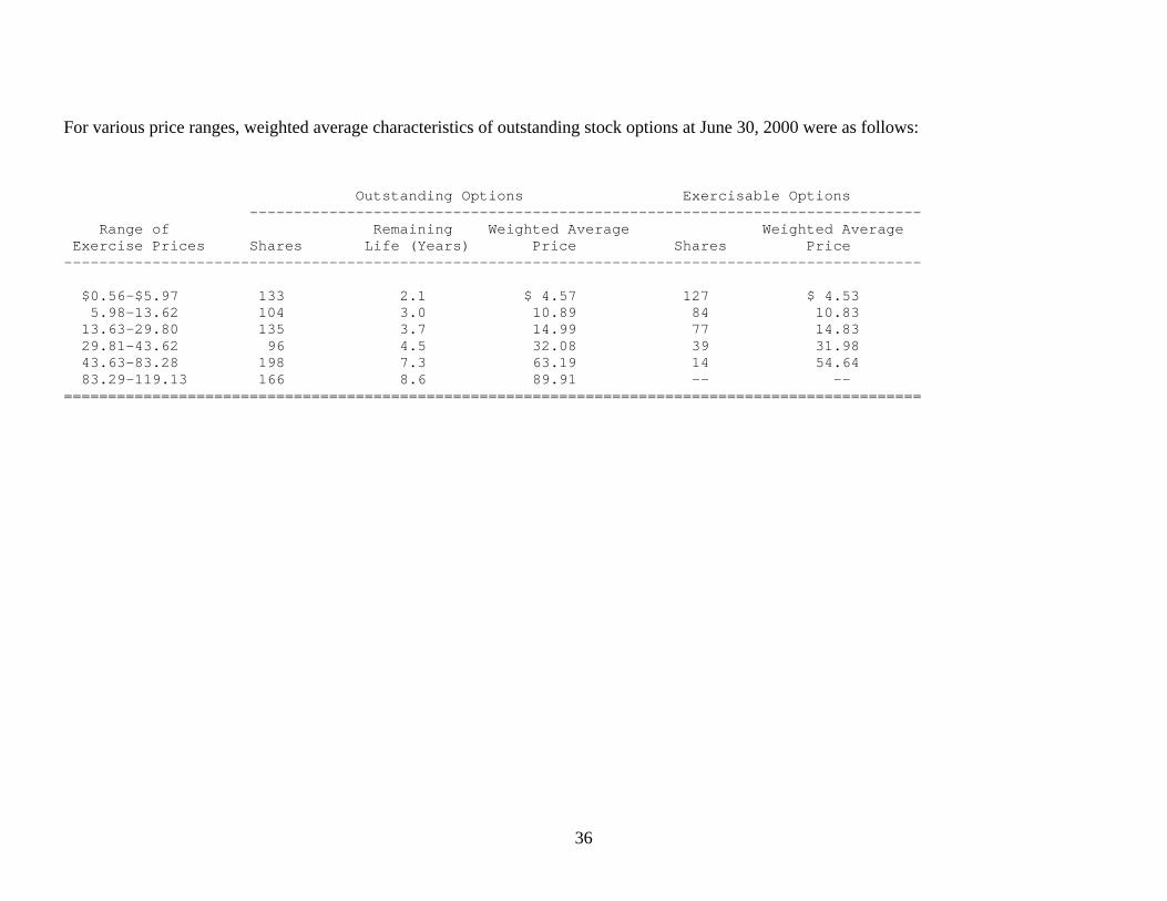
36

For various price ranges, weighted average characteristics of outstanding stock options at June 30, 2000 were as follows: Outstanding Options Exercisable Options ---------------------------------------------------------------------------- Range of Remaining Weighted Average Weighted Average Exercise Prices Shares Life (Years) Price Shares Price ------------------------------------------------------------------------------------------------- $0.56-$5.97 133 2.1 $ 4.57 127 $ 4.53 5.98-13.62 104 3.0 10.89 84 10.83 13.63-29.80 135 3.7 14.99 77 14.83 29.81-43.62 96 4.5 32.08 39 31.98 43.63-83.28 198 7.3 63.19 14 54.64 83.29-119.13 166 8.6 89.91 -- -- =================================================================================================

37

The Company follows Accounting Principles Board Opinion 25, Accounting for Stock Issued to Employees, to account for stock option and employee stock purchase plans. An alternative method of accounting for stock options is SFAS 123, Accounting for Stock-Based Compensation. Under SFAS 123, employee stock options are valued at grant date using the Black-Scholes valuation model, and this compensation cost is recognized ratably over the vesting period. Had compensation cost for the Company's stock option and employee stock purchase plans been determined as prescribed by SFAS 123, pro forma income statements for 1998, 1999, and 2000 would have been as follows: Year Ended June 30 1998 1999 2000 --------------------------------------------------------------------------------------------------------------------- Reported Pro Forma Reported Pro Forma Reported Pro Forma ------------------------------------------------------------------------------------ Revenue $15,262 $15,262 $19,747 $19,747 $22,956 $22,956 Operating expenses: Cost of revenue 2,460 2,603 2,814 3,013 3,002 3,277 Research and development 2,601 2,963 2,970 3,479 3,775 4,817 Acquired in-process technology 296 296 -- -- -- -- Sales and marketing 2,828 2,977 3,231 3,438 4,141 4,483 General and administrative 433 508 689 815 1,009 1,243 Other expenses 230 230 115 115 92 92 --------------------------------------------------------------------------------------------------------------------- Total operating expenses 8,848 9,577 9,819 10,860 12,019 13,912 --------------------------------------------------------------------------------------------------------------------- Operating income 6,414 5,685 9,928 8,887 10,937 9,044 Investment income 703 703 1,803 1,803 3,182 3,182 Gain on sales -- -- 160 160 156 156 --------------------------------------------------------------------------------------------------------------------- Income before income taxes 7,117 6,388 11,891 10,850 14,275 12,382 Provision for income taxes 2,627 2,369 4,106 3,741 4,854 4,210 --------------------------------------------------------------------------------------------------------------------- Net income $ 4,490 $ 4,019 $ 7,785 $ 7,109 $ 9,421 $ 8,172 ===================================================================================================================== Diluted earnings per share $ 0.84 $ 0.75 $ 1.42 $ 1.30 $ 1.70 $ 1.48 ===================================================================================================================== The weighted average Black-Scholes value of options granted under the stock option plans during 1998, 1999, and 2000 was $11.81, $20.90, and $36.67. Value was estimated using a weighted average expected life of 5.3 years in 1998, 5.0 years in 1999, and 6.2 years in 2000, no dividends, volatility of 0.32 in 1998 and 1999 and 0.33 in 2000, and risk-free interest rates of 5.7 percent, 4.9 percent, and 6.2 percent in 1998, 1999, and 2000.

38

TABLE I

Descriptive statistics on option characteristics All variables are from the Black-Scholes option valuation assumptions in the company financial statement footnotes. Expected life is years from grant until average exercise. The risk-free interest rate is the rate on zero-coupon U.S. government issues with remaining term equal to the expected life of the options. Dividend yield is dividends as a percentage of share price. Annual return volatility is the standard deviation of the continuously compounded rates of return on the stock (i.e., standard deviation of the difference in the natural logarithm of stock prices).

S&P 100 in 2000 Mean Median Std. Dev. 25th Perc. 75th Perc. Expected Life 5.22 5.00 1.64 4.15 6.43 Risk-Free Rate 6.10 6.20 0.50 5.88 6.46 Dividend Yield (%) 1.50 1.25 1.40 0.15 2.40 Annual Return Volatility 36.3 33.2 12.9 28.5 42.0

Nasdaq 100 in 2000 Mean Median Std. Dev. 25th Perc. 75th Perc. Expected Life 4.38 4.33 1.81 3.28 5.00 Risk-Free Rate 5.89 6.00 0.58 5.68 6.23 Dividend Yield (%) 0.09 0.00 0.48 0.00 0.00 Annual Return Volatility 73.2 72.0 25.7 55.0 91.5

39

TABLE II

Descriptive statistics on firm characteristics Asset is total assets. Market equity is the value of common equity at fiscal year-end. Return on assets is net income divided by assets. Debt/Value is total debt divided by the market value of the firm. Beta is the market-model beta as reported on CRSP.

S&P 100 in 2000

Mean Median Std. Dev. 25th Perc ddrc.75th Perc Perc.Asset ($M) 76,887 27,445 139,659 10,673 52,150 Market Equity ($M) 65,006 28,777 82,705 12,123 80,879 Return on Assets (%) 6.6 4.7 6.7 1.5 10.9 Debt/Value (%) 18.2 14.4 15.6 7.4 25.5 Beta 0.98 0.98 0.53 0.56 1.33

Nasdaq 100 in 2000 Mean Median Std. Dev. 25th Perc ddrc75th Perc Perc.Asset ($M) 7,074 2,457 13,087 1,432 6,803 Market Equity ($M) 22,435 8,885 44,045 5,351 18,133 Return on Assets (%) -0.2 5.3 38.3 -2.5 11.0 Debt/Value (%) 6.4 0.9 11.3 0.0 6.3 Beta 1.13 1.13 0.57 0.74 1.56

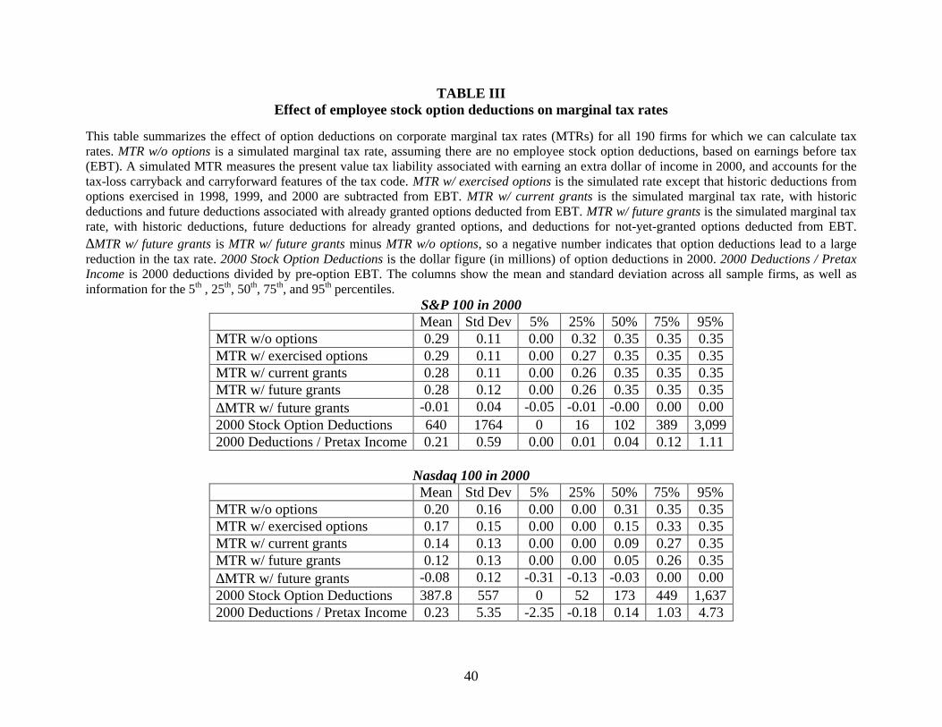
40

TABLE III Effect of employee stock option deductions on marginal tax rates

This table summarizes the effect of option deductions on corporate marginal tax rates (MTRs) for all 190 firms for which we can calculate tax rates. MTR w/o options is a simulated marginal tax rate, assuming there are no employee stock option deductions, based on earnings before tax (EBT). A simulated MTR measures the present value tax liability associated with earning an extra dollar of income in 2000, and accounts for the tax-loss carryback and carryforward features of the tax code. MTR w/ exercised options is the simulated rate except that historic deductions from options exercised in 1998, 1999, and 2000 are subtracted from EBT. MTR w/ current grants is the simulated marginal tax rate, with historic deductions and future deductions associated with already granted options deducted from EBT. MTR w/ future grants is the simulated marginal tax rate, with historic deductions, future deductions for already granted options, and deductions for not-yet-granted options deducted from EBT. ∆MTR w/ future grants is MTR w/ future grants minus MTR w/o options, so a negative number indicates that option deductions lead to a large reduction in the tax rate. 2000 Stock Option Deductions is the dollar figure (in millions) of option deductions in 2000. 2000 Deductions / Pretax Income is 2000 deductions divided by pre-option EBT. The columns show the mean and standard deviation across all sample firms, as well as information for the 5th , 25th, 50th, 75th, and 95th percentiles.

S&P 100 in 2000 Mean Std Dev 5% 25% 50% 75% 95% MTR w/o options 0.29 0.11 0.00 0.32 0.35 0.35 0.35 MTR w/ exercised options 0.29 0.11 0.00 0.27 0.35 0.35 0.35 MTR w/ current grants 0.28 0.11 0.00 0.26 0.35 0.35 0.35 MTR w/ future grants 0.28 0.12 0.00 0.26 0.35 0.35 0.35 ∆MTR w/ future grants -0.01 0.04 -0.05 -0.01 -0.00 0.00 0.00 2000 Stock Option Deductions 640 1764 0 16 102 389 3,099 2000 Deductions / Pretax Income 0.21 0.59 0.00 0.01 0.04 0.12 1.11

Nasdaq 100 in 2000

Mean Std Dev 5% 25% 50% 75% 95% MTR w/o options 0.20 0.16 0.00 0.00 0.31 0.35 0.35 MTR w/ exercised options 0.17 0.15 0.00 0.00 0.15 0.33 0.35 MTR w/ current grants 0.14 0.13 0.00 0.00 0.09 0.27 0.35 MTR w/ future grants 0.12 0.13 0.00 0.00 0.05 0.26 0.35 ∆MTR w/ future grants -0.08 0.12 -0.31 -0.13 -0.03 0.00 0.00 2000 Stock Option Deductions 387.8 557 0 52 173 449 1,637 2000 Deductions / Pretax Income 0.23 5.35 -2.35 -0.18 0.14 1.03 4.73

41

TABLE IV

Correlations between MTRs and leverage for combined sample of S&P 100 and Nasdaq 100 firms in 2000

Pearson (Spearman) correlations between corporate marginal tax rates and various measures of debt policy appear above (below) the main diagonal. MTR w/o options is a simulated marginal tax rate, assuming there are no employee stock option deductions, based on earnings before tax (EBT). MTR w/ future grants is the simulated marginal tax rate, with historic deductions, future deductions for already granted options, and deductions for not-yet-granted options deducted from EBT. ∆MTR w/ future grants is MTR w/ future grants minus MTR w/o options. Debt-to-value is total debt divided by the market value of the firm, where market value equals book assets minus book equity plus market equity. Debt-to-assets is total debt divided by total assets. Interest-to-value is debt interest divided by market value. Deductions-to-value is the dollar amount of option deductions in 2000 divided by market value. Kink in the proportion by which interest could be increased before the value of incremental interest deductions would begin to fall. Kink is calculated as in Graham (2000) using pre-option earnings. A high value for kink can be interpreted to mean that a firm has unused debt capacity (ignoring the effect of option deductions). These correlations are for the 156 firms included in the regression analysis. ***, **, * means statistically different from zero at the 0.01, 0.05, and 0.10 levels, respectively. Significance for the tax variables tests whether the correlation coefficient equals zero versus the alternative that the coefficient is greater than zero.

MTR w/o options

MTR w/ future grants

∆MTR w/ future grants

Debt-to-Value

Debt-to-Assets

Interest-to-Value

Deductions-to-Value

Kink

MTR w/o options

0.79***

-0.21***

0.04 0.03 -0.19*** -0.30*** 0.45***

MTR w/ future grants

0.74*** 0.44*** 0.23*** 0.12* 0.12* -0.56*** 0.26***

∆MTR w/ future grants

-0.01 0.48*** 0.30*** 0.15** 0.37*** -0.45*** -0.24***

Debt-to-Value 0.10 0.34*** 0.34*** 0.89*** 0.97*** -0.51*** -0.43*** Debt-to-Assets 0.09 0.26*** 0.22*** 0.89*** 0.81*** -0.39*** -0.24***

Interest-to-Value -0.08 0.25*** 0.50*** 0.97*** 0.81*** -0.54*** -0.59*** Deductions-to-

Value -0.25** -0.56*** -0.53*** -0.51*** -0.39*** -0.54*** 0.13*

Kink 0.43** 0.32** -0.16* -0.29*** -0.18** -0.49*** 0.08

42

TABLE V Tobit regressions of debt-to-value on marginal tax rates

and control variables

The dependent variable is Debt-to-value (total debt divided by book assets minus book equity plus market equity). MTR w/o options is a simulated marginal tax rate, assuming there are no employee stock option deductions, based on earnings before tax (EBT). MTR w/ exercised options is the simulated rate except that historic deductions from options exercised in 1998, 1999, and 2000 are subtracted from EBT. MTR w/ current grants is the simulated marginal tax rate, with historic deductions and future deductions associated with already granted options deducted from EBT. MTR w/ future grants is the simulated marginal tax rate, with historic deductions, future deductions for already granted options, and deductions for not-yet-granted options deducted from EBT. ∆MTR w/ future grants is MTR w/ future grants minus MTR w/o options. PP&E/Assets is property, plant, and equipment divided by total assets. Quick ratio is cash plus receivables, the sum divided by current liabilities. Cash Flow is operating cash flow divided by total assets. R&D is research and development expense divided by sales. Sales is sales revenue. Five significant 2-digit SIC code dummies are included in all specifications but are not shown in table. Regression coefficients and P-values (in parentheses) are shown. 1 2 3 4 5 6 7

Intercept 0.08 (0.01)

0.05 (0.01)

-0.00 (0.93)

0.01 (0.77)

0.03 (0.46)

0.04 (0.40)

0.04 (0.45)

MTR w/o options 0.07 (0.43)

0.13 (0.07)

0.22 (0.01)

MTR w/ exercised options

0.17 (0.03)

MTR w/ current grants

0.23 (0.01)

MTR w/ future grants 0.23 (0.01)

0.21 (0.01)

∆MTR w/ future grants

0.20 (0.05)

Lag PP&E / Assets 0.13 (0.01)

0.12 (0.03)

0.11 (0.05)

0.10 (0.06)

0.10 (0.06)

Lag Quick Ratio 0.01 (0.80)

0.01 (0.81)

0.00 (0.82)

0.01 (0.83)

0.01 (0.84)

Lag Cash Flow -0.49 (0.01)

-0.50 (0.01)

-0.49 (0.01)

-0.48 (0.01)

-0.49 (0.01)

Lag R&D -0.12 (0.04)

-0.13 (0.03)

-0.13 (0.03)

-0.13 (0.03)

-0.13 (0.03)

Lag Sales 0.01 (0.04)

0.01 (0.11)

0.01 (0.33)

0.01 (0.36)

0.01 (0.36)

n 156 156 147 147 147 147 147

43

TABLE VI More regressions of debt-to-value on marginal tax rates and control variables

The dependent variable is Debt-to-value (total debt divided by the market value of the firm, where market value equals book assets minus book equity plus market equity). MTR w/ future grants is the simulated marginal tax rate, with historic deductions, future deductions for already granted options, and deductions for not-yet-granted options deducted from EBT. MTR w/ future grants (Value Line) is the same simulated tax variable, based on stock price and growth projections from Value Line. S&P dummy is an indicator variable that takes on a value of one for S&P firms and 0 for Nasdaq firms. Stock Volatility is the volatility of stock returns. Option Deductions/Assets is the dollar value of tax deductions from employee stock options divided by total assets. Though not shown in the table, each regression includes PP&E/Assets, Quick ratio, Cash Flow, R&D, Sales, and five 2-digit SIC code dummies. Regression coefficients and P-values (in parentheses) are shown for the tax variable(s) and new control variables. The rightmost five columns summarize regressions that include, respectively, only firms that have nonzero debt, earnings greater than zero, an S&P bond rating, an investment grade bond rating, and growth larger than the mean growth in taxable income for the sample (3.6%). The four leftmost columns include all firms with nonmissing values for the explanatory variables. The regressions are all tobit specifications, except for the “Debt>0” column, which is OLS. ALL FIRMS FIRMS WITH Debt>0 Profits>0 Bond Rating Invest. Grade Growth>3.6%

MTR w/ future grants 0.16 (0.05)

0.19 (0.02)

0.15 (0.07)

0.21 (0.02)

0.22 (0.01)

0.27 (0.01)

0.35 (0.02)

0.20 (0.01)

MTR w/ future grants (Value Line)

0.21 (0.01)

S&P dummy 0.06 (0.01)

Stock Volatility -0.06 (0.24)

Option Deductions / Assets

-0.09 (0.10)

N

131

147

147

147

130

120

100

72

101

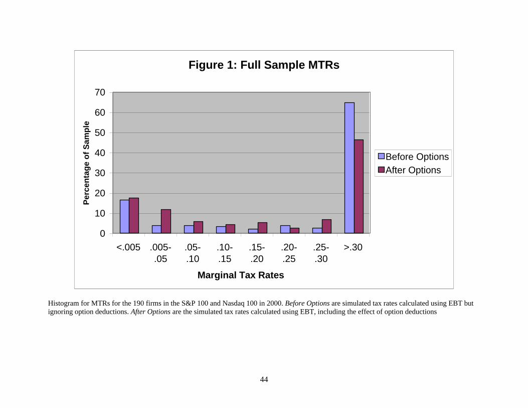
44

Figure 1: Full Sample MTRs

0

10

20

30

40

50

60

70

<.005 .005-.05

.05-.10

.10-.15

.15-.20

.20-.25

.25-.30

>.30

Marginal Tax Rates

Per

cen

tag

e o

f S

amp

le

Before OptionsAfter Options

Histogram for MTRs for the 190 firms in the S&P 100 and Nasdaq 100 in 2000. Before Options are simulated tax rates calculated using EBT but ignoring option deductions. After Options are the simulated tax rates calculated using EBT, including the effect of option deductions

45

Figure 2: NASDAQ 100 MTRs

0

10

20

30

40

50

60

<.005 .005-.05

.05-.10 .10-.15 .15-.20 .20-.25 .25-.30 >.30

Marginal Tax Rates

Per

cen

tag

e o

f S

amp

le

Before OptionsAfter Options

Histogram for MTRs for the firms in the Nasdaq 100 in 2000. Before Options are the simulated tax rates calculated using EBT but ignoring option deductions. After Options are the simulated tax rates calculated using EBT, including the effect of option deductions