NBER WORKING PAPER SERIES

TAXES AND FRINGE BENEFiTSOFFERED BY EMPLOYERS

William M. GentryEric Peress

Working Paper No. 4764

NATIONAL BUREAU OF ECONOMIC RESEARCH1050 Massachusetts Avenue

Cambridge, MA 02138June 1994

We are grateful to Michael Leber for helpful research assistance and Charlie Clotfelter, JonGruber, Gib Metcalf, Kip Viscusi and seminar participants at Duke University for usefulcomments. We thank Lee Hart of The Prudential for providing data on regional price factorsfor health insurance. This paper is part of NBER's research program in Public Economics.Any opinions expressed are those of the authors and not those of the National Bureau ofEconomic Research.

NBER Working Paper #4764June 1994

TAXES AND FRINGE BENEFITSOFFERED BY EMPLOYERS

ABSTRACT

Using cross-sectional data for blue and white collar workers for U.S. cities, we examine

how the tax treatment of fringe benefits affects whether employers offer benefits. Differences

in state-level income taxes cause variation across places in the tax incentives for fringe benefits.

We find that employers respond to tax incentives to offer fringe benefits, especially to blue collar

workers. The tax incentives affect both the probability of basic benefits, such as medical

coverage, and more "marginal" benefits, such as vision and dental coverage. Higher taxes also

reduce the amount of explicit cost sharing for some benefits between employers and employees.

William M. Gently Eric PeressDepartment of Economics Department of EconomicsBox 90097 Box 90097Duke University Duke UniversityDurham, NC 27708 Durham, NC 27708and NBER

Taxes and Fringe Benefits Offered by Employers

I. Introduction

In the current debate on reforming health care financing, both expanding and

curtailing tax-advantaged health insurance have been proposed.1 A key ingredient in

analyzing these proposals is the extent to which employer-provided benefits respond

to tax policy. U.S. tax law encourages firms to provide fringe benefits for which the

cost of the benefits are deductible to the employer but not taxable to the employee.

The tax incentives can work on two distinct margins. First, as hoped for by those

proposing more tax incentives, the tax treatment of fringe benefits encourages

employer-provided insurance plans. Therefore, increasing the tax incentives might

increase the number of insured Americans. Second, as feared by those wanting to

limit the tax-advantages for health insurance, once enrolled in an employer-provided

insurance plan, workers have an incentive to have generous insurance plans. This

extra insurance can come in several different forms: lower deductibles, lower

copayments, or coverage of more medical procedures. Overinsurance is one

explanation that has been given for the rapid increase in health care costs (see

Feldstein and Friedman, 1977).

To measure how fringe benefits respond to tax policy, we examine regional

variation in the percentage of workers offered different benefits (e.g., health insurance,

Editorials in The New York Times ("A Tax Cap for Health Reform, December 22, 1992)and The Washington Post (Who Pays for Health?," January 29, 1992) call for limiting the taxadvantage of fringe benefits. The Congressional Budget Office's (1994) report summarizessome of the possible changes in the tax system.

1

pensions, and dental insurance) from their employers. Since we have data on various

benefits, we can examine both the probability of basic health coverage and the

structure of additional benefits. The tax-advantage of fringe benefits varies within the

U.S. because state income tax rates vary across states. This regional variation in tax

rates helps to identity econometrically the relationship between taxes and fringe

benefits without some of the difficulties of using either time series data or data on

firms or individuals. We return to the econometric advantages of regional data below.

Our results suggest that tax incentives affect both the margin of how many

benefits or how much insurance firms offer rather as well as whether they offer basic

medical insurance. For example, for blue collar workers a one percentage point

increase in the tax rate increases the percentage of workers offered medical insurance

by 1 .8 percentage points and the percentage offered vision coverage by 1 .5

percentage points. However, since more than 90% of the workers in the sample are

offered basic medical coverage but only roughly one-third are offered vision coverage,

the effects of larger changes in tax incentives may be concentrated heavily on more

'marginal' benefits.

We also test whether the frequency of explicit cost sharing between employers

and employees depends on the tax rate. Since employee contributions do not always

receive the same tax advantage as employer contributions, higher tax rates encourage

firms to arrange compensation packages such that fringe benefits are entirely financed

by the firm. For blue collar workers, our results not only suggest that an increase in

personal tax rates increases the percentage of workers offered life insurance but also

2

induces a substitution of employer financing for employee contributions.

The paper is organized as follows. In section II, we discuss the incentive

effects of the tax treatment of fringe benefits and previous empirical studies relating

taxes and fringe benefits. In section III, we present our econometric model, discuss

the construction of our data, and consider the advantages of using regional-level data.

In section IV, we present our results. In section V, we conclude with a discussion of

the policy implications of our results.

II. The Taxation of Fringe Benefits and Previous Studies

A comprehensive income tax base would not distinguish between different

forms of compensation. In contrast, federal and state income tax systems exc'ude

some non-wage compensation from the individual income tax base. Excluded forms

of non-wage compensation include group medical insurance and life insurance. The

exclusion of these benefits from taxable income distorts workers' demand for different

types of compensation and, hence, different types of consumption. Furthermore, this

exclusion encourages the consumption of a particular good (fringe benefit) only if it is

financed in a particular fashion (through the employer-provided plan).

These benefits may be financed through employer contributions, employee

contributions (i.e., salary reductions) or a combination of the two. At the employer-

level, these benefits are taxed symmetrically to wages: employer contributions are

deductible from the firm's tax base. If the employer follows certain Internal Revenue

Service (IRS) rules, salary reductions allow employees to buy insurance without

3

paying income taxes on the cost of the insurance. For 1989, 25 percent of employees

who paid for part of their insurance were able to contribute pretax dollars (U.S. Bureau

of Labor Statistics, 1990). Even in plans with employee contributions, there are

substantial tax advantages since the employer pays the bulk of the premiums: for

irdividual coverage, Zedlewski (1992) estimates that 43 percent of employers pay the

entire premium and employers pay 85 percent of overall health insurance premiums.2

Combining these statistics suggests that employers who require some worker

contribution still pay 74 percent of total health insurance premiums.3 Thus, from the

employees perspective, both non-contributory (i.e., entirely employer-financed) plans

and contributory plans have significant tax advantages.

Since the employers contribution is deductible from the firm's taxable income,

the tax advantage for fringe benefits comes from the exclusion of employer

contributions and, in some cases, employee contributions from the employees taxable

income. The size of the tax advantage depends on the employee's marginal income

tax rate. For the portion of premiums that are excluded from taxable income,

employees face an effective price of insurance of one minus their marginal tax rate

times the price of the insurance. The tax adjustment, one minus the marginal tax rate,

2 One would expect that employer contributions to benefits would be offset by acompensating reduction in money wages. For a general survey on equalizing differences inwages, see Rosen (1986). Evidence on equalizing differences for employer-provided benefitsis mixed. In a recent example, Gruber (1992) finds a substantial wage offset using dataaround mandated changes in benefits.

That is, if workers in 43 percent of firms do not pay premiums, then workers in theremaining 57 percent of firms must pay 26 percent of their premiums for the averageemployer's share of premiums to equal 85 percent.

4

is commonly referred to as the "tax pnce" of the fringe benefit. With graduated

income tax rates, the tax advantage increases with the employee's income.

We focus on the employer's decision to offer a benefit in part because we

have data on benefits offered instead of the number of workers who actually take a

benefit. However, since the worker only gets the tax advantage if the employer oilers

the benefit, the decision whether to offer a benefit is an integral part of the tax effect.

The firm's decision to offer a benefit depends on the demands of its various workers.

The more workers who want a benefit, the more likely a firm is to offer the benefit.

Employee demand for a benefit depends on the marginal utility of receiving the

benefit. In turn, employee demand for employer-provided benefits, rather than buying

the benefit outside of the employer, depends on the size of the tax advantage and the

advantages of group policies. Since the tax advantage increases with the personal

tax rate, the pressure on a firm to offer a benefit should increase with the number of

workers with higher marginal tax rates. As the tax rate increases (either for all

workers of a firm or for a subset of workers), a firm would be more likely to offer a

benefit. Since employees at a firm face different tax rates and have different

preferences for insurance, a firm's decision to offer a benefit is a collective choice

problem (see Goldstein and Pauly, 1976). As discussed below, the collective choice

aspect of employer-provided benefits creates problems for measunng the tax

incentives facing a firm.

Previous empirical work on how the tax system affects fringe benefits

concentrates on three types of data: (1) time-series aggregate data; (2) cross-

5

sectional (or panel) data on firms; and (3) cross-sectional data on individuals. The

time-series studies (see, for example, Long and Scott, 1982, Vroman and Anderson,

1984, and Turner, 1 987b) typically find that the tax system encourages non-wage

compensation but the effect is relatively small. The major problem confronting time-

series analysis is controlling for non-tax factors that might affect the demand for fringe

benefits. For example, it is difficult to disentangle the variation in taxes from other

changes in supply and demand conditions for health insurance. Also, the time-series

approach is limited to a single tax rate for each year. Variation in this tax rate needs

to capture changing incentives at the firm-level for an employer to start offering a

fringe benefit. Since the firms decision depends on the demands of workers with

different incomes and tax rates, the amount of fringe benefits may depend on the

distribution of tax rates rather than just a measure of the average tax rate.

Relative to the time-series analyses, studies using cross-sectional data find that

taxes have economically significant effects on the choice between fringe benefits and

wages. The challenge for cross-sectional work is appropriately measuring variation in

tax incentives at either the firm or individual level. At the firm-level, the tax incentive

depends on the distribution of the employees' tax rates. Across firms, this tax

incentive varies because some firms have workers with higher tax rates than other

firms. Unfortunately, if one only considers federal taxes in a single year, employees'

tax rates across firms are determined by income levels of the employees. This

creates a standard problem for "tax price regressions": are the tax effects

econometrically identified with a single cross-section of data? Feenberg (1987)

6

discusses this problem for the case of charitable giving. Since tax rates are a non-

linear function of income, measured tax effects may really be non-linearities in how

income affects the demand for fringe benefits. Individual-level data suffer from the

same identification problem for tax effects and also ignores the public goods

dimension of fringe benefits: an employers decision to offer a benefit depends on the

tax rates of the individual and of the individual's co-workers.

Fortunately for studies of cross-sectional data, income tax rates vary by state.

This state-level variation is an important feature for econometrically identifying the tax

effects. Woodbury (1983), Adamche and Sloan (1985), Sloan and Adamche (1986),

Hirsch and Rufolo (1986), Turner (1987a) and Woodbury and Hamermesh (1992) all

use regional variation in tax rates to help identify their models.4 Each paper

incorporates state tax rates differently. For example, Turner imputes each family's

marginal total income tax rate (combining federal and state taxes) based on each

family's characteristics. In contrast, Woodbury and Hamermesh use the sum of the

marginal federal and state income and payroll tax rates for the median faculty member

at each college for which they have data. As discussed below, we use a similar

method for calculating the regional variation in marginal tax rates.

Turner (1987a) and Woodbury and Hamermesh (1992) are the closest

predecessors of our work. Following Turner, we go beyond examining the major

benefits (pensions, life and health insurance) to explore the margin of how many

' One alternative to regional variation in tax rates is changes over time in the Federal taxtreatment of health insurance premiums of the self-employed. Gruber and Poterba (1994)exploit this variation using a difterences-in-differences estimation strategy and find that thedemand for insurance is sensitive to tax-induced changes in the price of insurance.

7

benefits workers receive. Turner finds that taxes play a larger role in the number of

benefits rather than in the presence of the three major benefits. Like Turner, we

examine a variety of fringe benefits but we use aggregate data rather than a sample

of individuals which does not capture the effects of tax rates of each family's co-

workers. Aggregate data have the advantage of isolating the tax effect on the

employers decision rather than using tax rates of each family.

Woodbury and Hamermesh examine the employee benefits of academics

across the U. S. and find that the percentage of compensation received as fringe

benefits is responsive to the tax price of benefits. Like Woodbury and Hamermesh,

we explore the regional variation in fringe benefits and use differences in state tax

rates. Woodbury and Hamermesh use panel data which has the advantage of using

changes in federal tax rates to help identify tax effects. Relative to Woodbury and

Hamermesh, we use a broader sample of workers and focus on the percentage of

workers offered benefits rather than the percentage of compensation coming as fringe

benefits. More importantly, our data allow us to examine the composition of fringe

benefits rather than just the dollar value of benefits.

Ill. Empirical Model and Data

Most previous work with cross-sectional data tries to explain the variation in

either the dollar value or the share of non-wage compensation in total compensation.

We depart from this tradition in part because regional data on expenditures are not

available. Instead, we focus on the fraction of workers in a region who are offered

8

each benefit. The fraction of workers offered a benefit has at least one advantage

over expenditure data. Expenditures depend on the cost of the benefit which may

vary across places. However, workers who receive a benefit in a place where the

benefit is expensive may also place a higher dollar value on the benefit. This

endogeneity between the cost of the benefit and an individual's valuation of the benefit

may confound results based on cost measures of fringe benefits. For example, health

insurance prices may vary across regions because the cost of health care varies.

Employees in areas with high health care costs may value health insurance highly

because their potential medical care is expensive. The fraction of workers covered is

less susceptible to this endogeneity problem.

This study is unique in using regionally-aggregated data rather than national

aggregate, firm-level or individual data. By grouping employers within a labor market,

the variation in our data is from differences across labor markets rather than within a

labor market. Within a regional labor market, some employers may offer generous

benefits packages to attract workers who prefer non-wage compensation. Other firms

in the region may offer few benefits but compensate with higher wages. While tax

incentives would affect each firm's level of fringe benefits, benefits may vary within a

region as workers choose the firm with the wage and benefit package that best suits

their tastes. By using regional data, our approach captures how the tax system

affects the average level of benefits in the region.

The data on fringe benefits are from the U.S. Bureau of Labor Statistics' (BLS)

Occupational Compensation Surveys (formerly called Area Wage Surveys) for 1988-

9

1992. While the surveys come from different years, each region is surveyed once in

the five year penod. Most of the observations are city-level averages, though for less

populated states the unit of observation may be a region within the state or the whole

state. Unfortunately, earlier surveys do not include comparable information on fringe

benefits. The BLS surveys a sample of establishments with more than 50 worlers in

the region. The surveys include the percentage of blue and white collar workers

offered different fringe benefits. We use data on medical insurance, life insurance,

pensions, dental insurance, vision plans, coverage of hearing and drug or alcohol

rehabilitation. Some of these latter benefits can be provisions within the firm's medical

coverage. For the first three benefits, we also have information on whether the benefit

is financed entirely by the employer.5

We limit our analysis to a subset of the regions surveyed by the BLS for two

reasons. First, not all surveys include data on fringe benefits. Second, and more

importantly, we exclude regions that span more than one state or that might have a

substantial number of commuters from a different state (e.g., Washington D.C.).

Excluding these regions makes it easier to calculate the appropriate tax rate for each

region.

For each fringe benefit, we estimate separate least squares regressions for the

natural logarithm of the ratio of the odds of a worker being offered a benefit to the

As noted above, the tax rules for employee conthbuons to fringe benefits depend onwhether the firm's plans meet certain IRS rules. However, all workers covered by entirelyemployer-financed plans receive the tax advantage.

10

odds that a worker is not offered each benefit in the region.6 Using the "log-odds"

ratio, rather than the percent of workers offered a benefit, has the advantage that the

dependent variable is not truncated, so the error term does not violate assumptions of

the linear modeL The regression equation for each health-related fringe benefit is:

LN 100 = a + XkBk + PRICE1 + 3 PRlCE1TAX1 + (1)

where p1 is the percent of white or blue collar workers offered the benefit in the region,

Xi,, is a vector of k demographic variables, PRICE1 captures regional variation in the

cost of benefits, TAXi measures the tax advantage of fringe benefits, and is the error

term. Details on the explanatory vanables are below. The subscript i denotes regions

and the subscript k indexes the demographic variables. The coefficients to be

estimated are a, Bk (a vector), y, and 6, the effect of the tax incentive. The measure

of the tax incentive is interacted with the price variable since the after-tax cost of a

benefit is one minus the marginal tax rate times the price of the benefit. If taxes

encourage benefits, 6 would be positive.

Each observation in the regressions is weighted by:

e This iog-odds specification is the group data equivalent of a logit regression for data onindividual employees or firms. Of the 2352 region-benefit observations used in theregressions of equations (1) and (3), 14 observations had 100 percent of the workers coveredand 4 observations had 0 percent of workers covered. To prevent the logarithm of the oddsratio from being undefined, these observations are given values of 99.99 percent and 0.01percent.

11

POPweight = I

p(1 — pj

where POP is the 1990 population of the region. Weighting by population places

relatively more importance on more populated areas and corrects for

heteroscadasticity induced by each regions variables using different population sizes.

The weight includes p(l - p) to place less weight on observations that are near the

end of the possible range of probabilities. See Maddala (1983, p. 29) for details on

the econometric specification.

The main explanatory variable of interest is the tax incentive to compensate

workers with fnnge benefits instead of money. In constructing this variable, we want

to capture the regional variation in income tax rates. As discussed above, previous

papers emphasize the importance of state income taxes as a source of exogenous

variation in the tax incentives for employer-provided benefits. Since the tax incentive

for a given firm depends on the marginal tax rates of all of its employees, it is difficult

to create precise measures of the tax incentive.7 One advantage of using regional

data is that it is relatively easy to link regional data on fringe benefits with interstate

variation in income tax rates.

We use the total marginal tax rate at the state level for 1990. This tax rate is

One hypothesis is that firms respond to the demands of the workers as if the workerscould vote on whether the firm should otter a benefit. Under this framework, the tax rate ofthe decisive voter would be the critical tax rate for measuring the tax incentive facing the firm.The decisive voter may be the voter with median preferences (which with some addedrestrictions, would be the worker with the median income) or certain blocks of workers (e.g.,managers) may have more influence on the firm's decisions than other groups of workers.

12

the sum of the federal and state tax rates.8 We report results using tax rates

calculated for a representative household taken as a married couple with $40,000 of

state and Federal taxable income that itemizes its deductions. The tax rates capture

differences in state rates and state tax rules regarding the deductibility of Federal

income taxes from state taxable income. By assuming both Federal and state taxable

income of $40,000, our tax rates do not capture some subtle interstate differences in

the definition of taxable income. However, since these differences are unlikely to

change the marginal tax rate of the representative household,9 we believe our tax rate

estimates capture the regional variation in income taxes applying to wage income.

To measure the regional variation in the cost of health-related benefits, we

include area factors for calculating insurance premiums for small firms (fewer than fifty

employees) in each region.1° The area factors, denoted as PRICE1 in equation (1),

are adjustment factors for regional differences in the costs of buying a standard

See Bogart and Gentry (1992) for more details on the construction of state-level marginalincome tax rates (though their tax rates are specific to capital gains income). Unlike someprevious studies (Turner, 1987a and 1987b, and Woodbury and Hamermesh, 1992), we ignoreany incentives created from non-wage compensation being excluded from the payroll tax basefor Social Security for two reasons. First, it is unclear whether the payroll tax should beincluded because excluding fringe benefits from the payroll tax base also lowers future SocialSecurity benefits (see Sloan and Adamche, 1986). Second, since Social Security is a federalprogram, including the payroll tax would only change the level of the tax variable withoutaffecting the regional variation.

For example, for 1990, 30 of the 41 states with broad-based income taxes had topbrackets beginning at or below $30,000 (Advisory Commission on IntergovernmentalRelations, SiQnificant Features of Fiscal Federalism). Thus, fairly large changes in taxableincome would typically not change the representative household's marginal state tax rate.

° We are grateful to Lee Hart of The Prudential for providing this data. While larger firmsface similar variation in costs, they may negotiate individually with the insurance company orchoose to self-insure.

13

insurance policy. They control for region-specific differences in insurance company

loss ratios (ratio of claims to premiums) for health insurance after controlling for

differences iii industry, benefits included in the policy and demographics of the firm.

The firm pays a premium equal to the national premium times the area factor. The

area factors are for 1993 policies (historical data are not available). Area factors vary

by three-digit zip code. We include the area factors for the general delivery zip code

in the city or, when a general delivery zip code is not available, a centrally located zip

code in the region (or a large city within the region).

In addition to the tax variable, we control for various factors that might affect the

level of fringe benefits in a region. Since the age structure of the population may

affect demand for fringe benefits, we include the percent of the population between

the ages of 35 and 44 and the percent of the population between ages 55 and 64

from the 1990 Census. Under the hypothesis that a better educated workforce might

have a higher demand for fringe benefits, we include the percent of the population

over age 25 with more that twelve years of schooling in 1980 from the 1980 Census.

Since our dependent variable includes government workers, the fraction of the labor

force employed by the government might affect fringe benefits since government

workers are more likely to receive basic benefits packages than private sector workers

(see, for example, U.S. General Accounting Office, 1992). We include the state-level

fraction of manufacturing workers who belonged to a union in 1989 since unions have

typically bargained for more generous fringe benefits. Even though white collar

workers are less likely to unionize, we include this variable in the regressions for white

14

collar workers because of the collective choice nature of the decision to offer fringe

benefits.

Since the Occupational Compensation Surveys are staggered across years, we

include a set of dummy variables for the year of the survey to capture any national

level trends in fringe benefits. To avoid multicollinearity, we omit the year dummy for

1988. The staggered feature of the data also makes it difficult to measure consistently

the regional variation in the tax incentive for fringe benefits. Fortunately, there were

no major shifts in federal tax rates between 1988 and 1992. In order to get a

snapshot of the variation in state tax rates, we use tax rates for 1990. Two things

mitigate any adverse effects of using tax data from a single year. First, decisions

about fringe benefits are long-term decisions of employers. It is not practical for a firm

to change its benefits package every year. Thus, the fraction of workers offered a

benefit should respond to long-run tax incentives. Second, state tax systems rarely

change.

Since we do not have a price variable for life insurance and pensions, we

estimate the following equation without a price variable for these benefits:'1

p1LN =a+AkBk+öT/ucl÷c..100-p1

I

The hypothesis that higher tax rates increase employer-provided benefits suggests

that the coefficient on the tax variable should be positive.

Since all firms can invest pension contributions in the same capital markets, the price ofpension plans should not vary across regions. For life insurance, the cost could vary byregion or by firm depending on the age structure of the population. However, we do not haveestimates of regional variation in mortality.

15

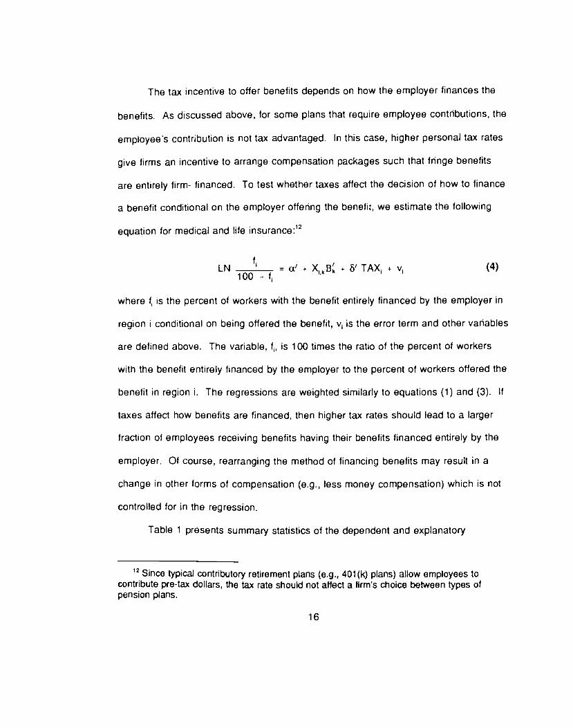
The tax incentive to offer benefits depends on how the employer finances the

benefits. As discussed above, for some plans that require employee contributions, the

employees contribution is not tax advantaged. In this case, higher personal tax rates

give firms an incentive to arrange compensation packages such that fringe benefits

are entirety firm- financed. To test whether taxes affect the decision of how to finance

a benefit conditional on the employer offering the benefit, we estimate the following

equation for medical and life insurance:12

LN a' + & TAX. + v (4)100-ft

where f, is the percent of workers with the benefit entirely financed by the employer in

region i conditional on being offered the benefit, v1 is the error term and other variables

are defined above. The variable, f, is 100 times the ratio of the percent of workers

with the benefit entirety financed by the employer to the percent of workers offered the

benefit in region i. The regressions are weighted similarly to equations (1) and (3). If

taxes affect how benefits are financed, then higher tax rates should lead to a larger

fraction of employees receiving benefits having their benefits financed entirely by the

employer. Of course, rearranging the method of financing benefits may result in a

change in other forms of compensation (e.g., less money compensation) which is not

controlled for in the regression.

Table 1 presents summary statistics of the dependent and explanatory

12 Since typical contributory retirement plans (e.g., 401(k) plans) allow employees tocontribute pre-tax dollars, the tax rate should not affect a firm's choice between types ofpension plans.

16

variables. Typically, a higher percentage of white collar workers receive a benefit than

blue collar workers, though anti-discrimination rules prevent the differences from being

too large. Across the two types of workers, the pattern of benefits offered is similar:

health insurance and life insurance are the most common benefits while vision and

hearing coverage are the least common.

IV. Results

Blue Collar Workers. In table 2, we present estimates of equation (1) for

health-related benefits and equation (3) for non-health-related benefits for blue collar

workers. For nine of the ten regressions (the exception is hearing coverage), the

coefficient on the tax variable is positive and statistically significant at the five percent

significance level (using a two-tailed test) in eight of the regressions indicating that the

income tax system encourages fringe benefits. In the log-odds specification, the effect

of changing an exogenous variable on the probability of benefit coverage depends on

the level of the probability.'3 We evaluate the effects of exogenous variables at the

mean probability of each benefit. Evaluated at the mean area factor (price) of 0.67, a

one percentage point reduction in the marginal tax rate would reduce the percentage

of workers offered medical insurance by 1.84 percentage points, dental insurance by

1.18 percentage points, vision coverage by 1.47 percentage points, and drug and

alcohol abuse treatment by 0.56 percentage points. Thus, taxes affect both basic

' A change in an exogenous variable changes the probability by approximately thecoefficient multiplied by the probability times one minus the probability. Thus, a unit change inan exogenous variable affects a low or high probability by less than a probability that is closeto 0.5.

17

benefits and the degree of generosity of the benefits pacKage.

In addition to the tax effects on health-related benefits, the results indicate that

the tax rate affects how many workers are offered life insurance and pension benefits.

A one percentage point increase in the tax rate increases the percentage of workers

offered life insurance by 0.83 percentage points and the percentage offered pension

plans by 0.89 percentage points. Taxes have a larger effect on the percentage of

workers offered life insurance and pensions entirely financed by the firm: a one

percentage point increase in the tax rate increases the percentage of workers with

employer-financed life insurance by 1.21 percentage points and employer-financed

pensions by 1.33 percentage points. We return to the differences between

contnbutory and non-contributory plans in the discussion of table 4.

Overall, the model explains a considerable portion of the regional variation in

employer-offered benefits. The adjusted R2's range from 0.26 to 0.79. The

coefficients on other variables in the regressions conform with their expected signs

and some are statistically significant. For example, The percent of workers offered

benefits typically increases with unionization at the state level. The coefficient on price

is negative except for the hearing benefits regression. For medical insurance, a one

standard deviation increase in the area factor, reduces the percent of blue collar

workers offered health insurance by 6.3 percentage points which suggests that firms'

decisions to offer benefits are sensitive to the cost of the benefits.'4

This change is evaluated at the mean percent offered medical benefits and the meantax rate.

18

White Collar Workers. Table 3 has results for equations (1) and (3) for white

collar workers. Relative to the results for blue collar workers, these results do not lend

strong support to the hypothesis that taxes are important determinants of whether

firms offer fringe benefits. While seven of the ten coefficients on the tax variables are

positive, the coefficients for white collar workers are typically not statistically significant

at the five percent level. All of the tax coefficients except one are smaller (in absolute

value) than their counterparts for blue collar workers. Furthermore, the regressions for

white collar workers have less explanatory power than the regressions for blue collar

workers, as evidenced by the lower adjusted R2s for most of the benefits.

Overall, the results suggest that taxes may be less important for white collar

workers than for blue collar workers and variables other than those included in the

regressions may be important for white collar workers. Since white collar workers are

more likely to have higher tax rates than blue collar workers, it is surprising that the

tax variable is more important for blue collar workers. However, varying the income

level (and hence tax rate) of the representative household does not reverse this

pattern. One possible explanation of the lower predictive power for white collar is that

white collar workers are a smaller, more diverse group of employees within each

region.

Sensitivity Analysis. These results are robust to wo types of alternative

specifications. To conserve space, we do not report these results in tables. First, to

explore the validity of our measure of the price of health benefits, we estimated

different specifications of equation (1). For health-related benefits, the qualitative

19

results are similar for regressions without the price variable (i.e., equation (3)) and for

regressions with separate price and tax variables but no interaction between the two

variables.

Second, to check whether the tax variable captures regional variation in income

taxes, we used two types of alternative tax variables: (1) we constructed marginal tax

rates for alternative representative households; and (2) state income tax collections

per $100 of state personal income for 1990 (from the Advisory Commission on

Intergovernmental Relations' Significant Features of Fiscal Federalism). Specifically,

we considered three different representative households: (1) a family of four with

adjusted gross income of $35,000 taking the standard deduction and exemptions; (2)

a single person with adjusted gross income of $28,000 taking the standard deduction;

and (3) a family with itemized deductions and taxable income of $100,000. The

second alternative tax variable is an average state income tax rate. Replacing the

marginal tax rate for families with $40,000 of taxable income in equations (1) and (3)

with these alternative tax variables yields qualitatively similar results to those in tables

2 and 3 although the coefficients are less statistically significant with the average tax

rate measures.15

Financing Major Fringe Benefits. Since in some plans employee

contributions are not tax-advantaged, higher personal income tax rates give employers

an incentive to use non-contributory plans to provide benefits. Therefore, conditional

IS Since the state average tax rate is not a total of Federal and state taxes, for theregressions with the average tax rate, we estimated a model with the separate price and taxvariables without an interaction.

20

on a firm offering benefits, higher tax rates should increase the chance that a firm

either meets the IRS rules for employee contributions to be tax-advantaged or to not

require employee contributions for benefits. Table 4 presents the regression results

from equation (4) for medical and life insurance.

For blue collar workers, the tax rate coefficient is statistically insignificant for

medical insurance but positive and statistically significant at the five percent

significance level for life insurance. These results indicate that an increase in income

tax rates induces a substitution from contributory plans to non-contnbutory plans for

life insurance. For example, a one percentage point increase in the tax rate increases

the percentage of workers whose life insurance is entirely financed by the employee

by 1 .6 percentage points. Recall from table 2 that an increase in the tax rate

increases the likelihood of coverage for both medical and life insurance for blue collar

workers. This substitution is in addition to the increased frequency of benefits. This

substitution suggests that higher taxes reduce the amount of explicit cost sharing

between employees and employers for benefits. The lack of cost sharing between

employees and employers may contribute to rapidly increasing health care costs. The

unionization variable has a statistically significant positive effect on the fraction of firms

that entirely finance benefits.

For white collar workers, the tax rate coefficient for neither medical nor life

insurance is statistically significant. The explanatory power of the regressions for

white collar workers is much lower than that of the regressions for blue collar workers.

As with the results in tables 2 and 3, taxes seem more important for blue collar

21

workers than white collar workers. Also consistent with the results in tables 2 and 3,

the results are robust to using alternative measures of the tax incentives.

V. Policy Implications and Conclusion

Using regionally-aggregated data on fringe benefits offered by employers and

interstate variation in tax rates, we offer new evidence on the effects of income taxes

on the level of fringe benefits offered by employers. Overall, our results are consistent

with previous cross-sectional studies of the effects of taxes on fringe benefits. Unlike

other studies (except Turner, 1987a), we identify both the margin of whether an

employer offers basic benefits and the margin of how many benefits the employer

offers. Taxes seem important on both margins. We also estimate whether taxes

affect how firms elect to finance fringe benefits and whether taxes affect the amount of

explicit cost sharing between employers and employees. Our main empirical findings

are:

Higher income taxes increase the utilization of fringe benefits. This increase isboth economically and statistically significant for blue collar workers. Theresults are less pronounced for white collar workers.

Taxes have a similar effect on "rnarginar' benefits such as vision coverage anddental insurance and whether workers are offered basic medical insurance.

Higher income taxes induce some substitution from contributory plans withexplicit cost sharing towards non-contributory (entirely employer-finance) planswith no explicit cost sharing. This substitution is consistent with firms financingfringe benefits in a way that minimizes their employees' taxes.

Our estimates suggest that tax rates affect the level and types of benefits

22

offered by employers as well as the choice of how these benefits are financed. Many

current proposals are geared at limiting or capping the tax advantages of fnnge

benefits. These proposals call for either a limited exclusion (or credit) of fringe

benefits at the level of the personal income tax or a cap on the amount that employers

àan deduct for fringe benefits per employee from firm level income. The advantage of

these proposals is that they maintain a tax subsidy for basic medical insurance without

subsidizing excessive fringe benefits. Since our results suggest that taxes affect both

basic benefits as well as more "marginal' benefits, these policies may curtail the

offering of more "marginal" fringe benefits without greatly influencing how many people

are offered basic coverage. While we cannot offer direct evidence on the levels of

copayments and deductibles, the results are consistent with these policies affecting

the amount of insurance individuals have, rather than whether individuals have any

insurance at all. However, our results are estimated using a relatively small amount of

variation in the tax rates, so it is difficult to extrapolate the effects of these proposals

since these policies may have substantial effects on the pre-tax price of insurance and

medical care. With this caveat in mind, the results suggest that these policies would

have their intended effect of reducing the number of people with overly generous

benefits packages: the alternative policy of eliminating the special tax treatment of all

fringe benefits might affect the how many people receive basic coverage.

23

References

Adamche, Killard, and Frank Sloan, 1985, "Fringe Benefits: To Tax or Not To Tax?,"National Tax Journal 36, 47-64,

Bogart, William 1. and William M. Gentry, 1992, 'Capital Gains Taxes andRealizations: Evidence From Interstate Comparisons," National Bureau ofEconomic Research Working Paper #4254, Cambridge, MA.

Congressional Budget Office, 1994, IjTreatmentof Emiloyment-Based HealthInsurance, Government Printing Office: Washington, D.C.

Feldstein, Martin S. and Bernard Friedman, 1977, "Tax Subsidies, the RationalDemand for Insurance, and the Health Care Crisis," Journal of PublicEconomics 7, 155-1 78.

Feenberg, Daniel, 1987, "Are Tax Price Models Really Identified: The Case ofCharitable Giving," National Tax Journal 40, 629-633.

Goldstein, Gerald S. and Mark V. Pauly, 1976, "Group Health Insurance as a LocalPublic Good," in Richard N. Rosett, ed., The Role of Health Insurance JniHealth Services Sector, New York: National Bureau of Economic Research, 73-110.

Gruber, Jonathan, 1992, "The Incidence of a Group-specific Mandated Benefit:Evidence from Health Insurance Benefits for Maternity," National Bureau ofEconomic Research Working Paper #41 57, Cambridge, MA.

Gruber, Jonathan, and James M. Poterba, 1994, "The Elasticity of Demand for HealthInsurance: Evidence from the Self-employed," Quarterly Journal of Economics,forthcoming.

Hirsch, Werner Z., and Anthony M. Rufolo, 1986, "Effects of State Income Taxes OnFringe Benefit Demand of Policemen and Firemen," National Tax Journal 39,211-220.

Long, James E., and Frank A. Scott, 1984, "The Impact of the 1981 Tax Act on FringeBenefits and Federal Revenues," National Tax Journal 37, 185-194.

Maddala, G. S., 1983, Limited-DeDendent and Qualitative Variables in Econometrics,New York: Cambridge University Press.

Rosen, Sherwin, 1986, "The Theory of Equalizing Differences," in Orley Ashenfelterand Richard Layard, eds., Handbook of Labor Economics, Amsterdam:

24

Elsevier Science Publishers.

Sloan, Frank, and Killard W. Adamche, 1986, 'Taxation and the Growth of Non-WageCompensation," Public Finance Quarterly 14, 115-137.

Turner, Robert W., 1987a, "Taxes and the Number of Fringe Benefits Received,"Journal of Public Economics 33, 41-57.

Turner, Robert W., 1987b, "Are Taxes Responsible for the Growth in Fringe Benefits?"National Tax Journal 40, 205-221.

U.S. Bureau of Labor Statistics, 1990, Employee Benefits in Medium and LargeFirms, 1989.

U.S. Bureau of Labor Statistics, Occupational Compensation Survey, Multiple issues1988-1992.

U.S. General Accounting Office, 1992, Tax Policy: Effects of Changing the TaxTreatment Fringe Benefits, Washington D.C.: Government Printing Office.

Vroman, Susan, and Gerard Anderson, 1984, "The Effect of Income Taxation on theDemand for Employer-Provided Health Insurance," Applied Economics 16, 33-43.

Woodbury, Stephen A., 1983, "Substitution Between Wage and Nonwage Benefits,"American Economic Review 73, 166-182.

Woadbury, Stephen A., and Daniel S. Hamermesh, 1992, "Taxes, Fringe Benefits, andFaculty," Review of Economics and Statistics 74, 287-296.

Zedlewski, Shelia A., 1992, "Expanding the Employer-Provided Health InsuranceSystem: Effects on Workers and Their Employers," in Health Benefits iti.Workforce, U.S. Department of Labor, 169-194.

25

</ref_section>

Table 1: Summary Statistics

Mean Stan. 0ev. Minimum Maximum

Fringe Benefits: Blue Collar

Health Insurance 89.4 8.4 61 100

Health Entirely Firm-Funded 48.5 15.4 14 84

Dental 67.2 15.4 16 93

Vision 33.6 18.9 1 75

Hearing 19.8 14.4 0 62

Drug/Alcohol 80.5 10.7 53 99

Life Insurance 89.6 6.4 67 99

Life Entirely Firm-Funded 73.1 11.5 40 94

Pension 67.4 13.5 40 93

Pension Entirely Firm-Funded 59.6 14.3 28 87

Fringe Benefits: White Collar

Health Insurance 95.9 5.7 72 100

Health Entirely Firm-Funded 46.0 14.2 20 85

Dental 76.6 157 22 98

Vision 34.6 19.6 0 79

Hearing 18.3 14.6 0 65

Drug/Alcohol 86.9 11.2 50 99

Life Insurance 96.0 4.8 61 100

Life Entirely Firm-Funded 81.9 10.0 42 98

Pension 78.7 12.3 35 98

Pension Entirely Firm-Funded 70.4 12.8 33 94

Explanatory Variables

Marginal Tax Rate 0.311 0.0193 0.28 0.345

Population Ages 35-44 15.2 1.3 11.3 18.7

Population Ages 55-64 8.1 1.2 4.5 11.0

Govl workers per 100 6.76 2.54 4.12 16.54

Unionization 19.9 12.7 2.4 51.6

High School Education 69.1 7.7 41.3 83.7

Area Factors for Health Ins. 0.67 0.28 0.37 2.12

26

Table 2: Fringe Benefits for Blue Collar Workers Dependent Vanable: Ln(p/(100 - pj) where p = percentage of woricers oflered each benefit

Medical Medical from firm

Dental Vision Heanng Drug & Alcohol

Life Life from tirm

Pension Pension from firm

Constant 10,03' (2.92)

-1.50 (0.77)

-2.36' (0.89)

-6.35' (1.14)

-19.35' (1.64)

-2.31

(1.20) -1.46 (1.67)

-2.79' (1.12)

-2.77' (1.11)

-2.99' (1.05)

Pop35 -0.035 (0.17)

0.15' (0.043)

0.076 (0.049)

0.13' (0.066)

0.70' (0.11)

0.10 (0.067)

0.062 (0.065)

0.070 (0.045)

0.037 (0.044)

0.053 (0.042)

Pop55 0.15 (0.18)

-0.029 (0.045)

-0.133' (0.053)

-0.093 (0.069)

0.37' (0.12)

0.036 (0.071)

0.24' (0.071)

0.090 (0.048)

0.12' (0.047)

0.11' (0.045)

Educatl2 -0.064' (0.029)

-0.0040 (0.008)

0.048' (0.009)

0.051' (0.012)

0.021

(0.021) 0.030'

(0.012) -0.019 (0.012)

0.0001 (0.008)

-0.0068 (0.008)

-0.0018 (0.008)

Govt workers

-0.098 (0.085)

-0.022 (0.023)

-0.077' (0.026)

-0.072' (0.035)

0.13' (0.066)

-0.051

(0.034) 0.042

(0.031) 0.0020

(0.022) 0.0082

(0.022) -0.0063 (0.021)

Union89 -0.018 (0.015)

0.028' (0.004)

0.020' (0.005)

0.027' (0.007)

0.041' (0.013)

0.018' (0.006)

0.0044 (0.006)

0.023' (0.004)

0.028' (0.004)

0.026' (0.004)

Price -11.38' (3.91)

-2.90' (0.96)

-2.30 (1.17)

-2.47 (1.56)

1.50 (2.82)

-2.23 (1.56)

Price • Tax 28.94 (12.24)

8.07' (3.04)

7.97' (3.64)

9.86 (4.90)

-2.15 (9.12)

5.29 (4.82)

Tax Rate 5.88' (3.84)

6.16' (2.62)

4.03' (2.60)

5.52' (2.48)

#otobs. 108 108 108 108 105 107 108 108 108 108

Adj. R2 0.28 0.57 0.53 0.52 0.79 0.26 0.35 0.40 0.47 0.49

Coefliaents are estimated using weighted least squares with the weights described in the text. denotes coefficients that differ from zero at the 5 percent significance level (two-tailed test). The regressions also include year dumnies for the year of the survey.

27

Table 3: FrInge Benefits for White Collar Workers Dependent Vanable: Ln(p/(100 - pt)) where p percentage of woricers ottered each benefit

Medical Medical from finn

Dental Vision Hearing Drug & Alcohol

Life Life from firm

Pension Pension from firm

Constant 9.45' -0.93 -359' -17.92' -24.17' -204 -1.16 -1.58 -2.25 -1.72 (3.95) (0.90) (1.33) (2.17) (2.26) (1.45) (4.18) (1.65) (1.35) (1.25)

Pop35 0.15 0.075 0.072 0.43' 0.59' 0.15 0.19 0.038 -0.0020 0.048 (0.22) (0.049) (0.072) (0.14) (0.14) (0.081) (0.15) (0.066) (0.053) (0.050)

Pop55 0.35 -0.054 -0.11 -0.16 0.10 -0.0028 0,38' 0.12 0.14' 0.13' (0.22) (0.052) (0.079) (0.15) (0.16) (0.081) (0.17) (0.070) (0.057) (0.053)

Educatl2 -0.086' -0.0015 0.064' 0.12 0.11* 0.029' -0.040 0.012 0.017 -0.0043 (0.039) (0.009) (0.013) (0.024) (0.027) (0.014) (0.029) (0.012) (0.010) (0.009)

Govt -0.063 0.059' -0.031 -0.0046 0.067 -0.070 -0.018 0.016 0.045 -0.0014 workers (0.11) (0.026) (0.038) (0.077) (0.091) (0.041) (0.074) (0.031) (0.025) (0.025) Union89 0.051 O.013 O.014 0.029' 0.073' 0.021' 0.043' 0.018' 0.027' 0.019'

(0.017) (0.005) (0.007) (0.014) (0.016) (0.008) (0.014) (0.006) (0.005) (0.005) Price -11.50' 0.80 0.16 2.27 10.53 -0.63

(5.46) (1.16) (1.70) (3.51) (3.97) (1.81) Pnce • Tax 23.29 -1.87 1.65 -4.18 -30.25' 1.63

(17.38) (3.65) (5.27) (11.01) (12.75) (5.55) Tax Rate 8.66

(9.43) 2.51

(3.82) 2.98

(3.18) 2.07

(2.95)

#ofobs. 108 108 108 108 105 107 108 108 108 108

Adj. A2 0.44 0.28 0.38 0.67 0.70 0.25 0.32 0.16 0.40 0.35

Coeffiaents are estimated using weighted least squares with weights described in the text. 'denotes coefficients that differ from zero at the 5 percent sigrvficance level (two-tailed test). The regressions also Include year dummies for the year of the survey.

28

Table 4: Form of Financing Fringe BenefitsDependent Variable: Ln(f/(100 - f)

where f, looPercentage of workers offered benefit entirely financed by firm divided bythe percentage of workers offered benefit

,

Blue Collar White Collar

Medical Life Medical Life

Constant -0.51

(0.90)2.26*(1.06)

-0.62(1.39)

1.15(1.83)

Pop35 0.12(0.046)

0.052(0.054)

0.11

(0.055)0.12

(0.072)

Pop55 -0.046(0.042)

-0.054(0.050)

-0.12(0.057)

-0.026(0.075)

Educatl2 -0.0039(0.0063)

-0.0010(0.0074)

-0.0089(0.0090)

-0.0087(0.012)

Govt workers -0.039(0.026)

-0.090(0.030)

0.025(0.030)

0.0015(0.039)

Unton89 0,028(0.0048)

0.035*(0.0056)

0.011

(0.0050)0.026

(0.0066)

Tax Rate -0.66(2.72)

1O.96

(3.20)1.92

(3.23)-2.56(4.25)

#ofobs. 108 108 108 108

Adj. A2 0.51 0.51 0.19 0.11

Coefficients are estimated using weighted least squares as described in the text. • denotes coefficientsthat differ from zero at the 5 percent significance level (two-tailed test). The regressions also includeyear dummies for the year of the survey.

29