NBER WORKING PAPER SERIES

EXPORT VERSUS FDI

Elhanan HelpmanMarc J. Melitz

Stephen R. Yeaple

Working Paper 9439http://www.nber.org/papers/w9439

NATIONAL BUREAU OF ECONOMIC RESEARCH1050 Massachusetts Avenue

Cambridge, MA 02138January 2003

The statistical analysis of firm level data on U.S. Multinational Corporations reported in this study wasconducted at the International Investment Division, U.S. Bureau of Economic Analysis, under arrangementthat maintained legal confidentiality requirements. Views expressed are those of the authors and do notnecessarily reflect those of the Bureau of Economic Analysis. Elhanan Helpman thanks the NSF for financialsupport. We also thank Daron Acemoglu, Roberto Rigobon,Yona Rubinstein and Dani Tsiddon for commentson an earlier draft, and Man-Keung Tang for excellent research assistance. The views expressed herein arethose of the authors and not necessarily those of the National Bureau of Economic Research.

©2003 by Elhanan Helpman, Marc J. Melitz, and Stephen R. Yeaple. All rights reserved. Short sections oftext not to exceed two paragraphs, may be quoted without explicit permission provided that full creditincluding . notice, is given to the source.

Export versus FDI Elhanan Helpman, Marc J. Melitz, and Stephen R. YeapleNBER Working Paper No. 9439January 2003JEL No. F12, F14, F23, L11

ABSTRACT

This paper builds a multi-country, multi-sector general equilibrium model that explains the decisionof heterogeneous firms to serve foreign markets either through exports or local subsidiary sales(FDI). These modes of market access involve different relative costs, some of which are sunk whileothers vary with sales volume (such as transport costs and tariffs). Relative to investment in asubsidiary, exporting involves lower sunk costs but higher per-unit costs. In equilibrium, only themore productive firms choose to serve the foreign markets and the most productive among thisgroup will further choose to serve the overseas market via FDI. The paper then explores severalimplications of the individual firms’ decisions for aggregate export and FDI sales relative to thedomestic and foreign market sizes. In particular, it is shown that firm level heterogeneity is animportant determinant of relative export and FDI flows.

We use the model to derive testable empirical predictions on the relative aggregate export and FDIsales in a given country for a given sector based both on relative costs and the extent of firm levelheterogeneity in that sector. These predictions are tested on data of US affiliate sales and USexports in 38 different countries and 52 sectors. The comparative statics based on relative costs arevery similar to those tested by Brainard (AER 1997) and are confirmed in our data: sector/countryspecific transport costs and tariffs have a strong negative effect on export sales relative to FDI.More importantly, our new predictions for the effects of firm-level heterogeneity on the relativeexport and FDI sales are also strongly supported by the data: more heterogeneity leads tosignificantly more FDI sales relative to export sales.

Elhanan HelpmanDepartment of EconomicsHarvard UniversityCambridge, MA 02138and NBERehelpman@harvard.edu

Marc J. MelitzDepartment of EconomicsHarvard UniversityCambridge, MA 02138and NBERmmelitz@harvard.edu

Stephen R. YeapleDepartment of EconomicsUniversity of Pennsylvania3718 Locust WalkPhiladelphia, PA 19104-6297snyeapl2@econ.upenn.edu

1 Introduction

Multinational sales have grown tremendously in the last two decades. Growth of these

sales has even outpaced the remarkable expansion of trade in manufactures. Conse-

quently, the trade literature has sought to incorporate the mode of foreign market

access into the “new” trade theory. This literature recognizes that firms can service

foreign buyers through a variety of channels: they can export their products to for-

eign customers, serve them through foreign subsidiaries by engaging in foreign direct

investment (FDI), and license or contract with foreign firms to produce and sell their

products.

Our work focuses on the firm’s choice between exports and “horizontal” FDI.1

Horizontal FDI refers to investments in production facilities abroad that are designed to

serve foreign customers. We therefore exclude “vertical” motives for FDI, that involve

fragmentation of production across countries.2 We follow the previous literature on

horizontal FDI in assuming that foreign affiliate production is intended for the host

country market.3 However, we show in an appendix how our model can be extended

to incorporate exports by foreign affiliates. This adds a new motive for FDI: the use of

affiliates as “export platforms.” In all these cases, however, firms invest abroad when

the gains from avoiding transport costs outweigh the costs of maintaining capacity in

multiple markets. This is known as the proximity—concentration tradeoff.

We extend the proximity—concentration tradeoff literature by introducing intra-

industry firm heterogeneity. We build a simple multicountry, multisector general equi-

librium model that explains the decisions of heterogeneous firms to serve foreign mar-

kets through exports or local subsidiary sales. These modes of market access have

different relative costs, some of which are sunk (such as entry costs) while others vary

1See Ethier (1986), Horstmann and Markusen (1987), and Ethier and Markusen (1996) for modelsthat incorporate the licensing alternative.

2An example of vertical FDI is when a parent firm invests in a production facility in anothercountry in order to produce inputs that will be shipped back to the parent for further processing. Orwhen a parent firm produces only inputs in the home country and it invests in an assembly facilityin another country to which it ships these inputs. See Helpman (1984), Helpman (1985), Markusen(2002, Ch. 9), and Hanson, Mataloni and Slaughter (2002) for treatments of this form of FDI.

3See, for example, Horstmann and Markusen (1992), Brainard (1993), and Markusen and Venables(2000).

1

with sales (such as transport costs and tariffs). Relative to FDI, exporting involves

lower sunk costs but higher per-unit costs.4

We show that firm heterogeneity in productivity plays an important role in explain-

ing the structure of international commerce. First, only the most productive firms

engage in foreign activities. This result mirrors other findings on firm heterogeneity

and trade, in particular, the results reported in Melitz (2002).5 Second, of those firms

that serve foreign markets, only the most productive engage in FDI.6 Third, the extent

of intra-industry firm heterogeneity plays a key role in determining the volume of FDI

sales relative to the volume of exports. Hence, we identify a new industry character-

istic – the dispersion of productivity levels across firms – as a determinant of the

composition of trade.

This allows us to derive new insights from the proximity—concentration tradeoff.

First, standard proximity—concentration variables determine the productivity levels

that a firm must achieve to make its international activities attractive. But these

productivity levels do not fully determine the composition of trade; they have to be

combined with information about the degree of dispersion of productivity levels across

firms within every industry in order to forecast trade flows.7 Second, our model avoids

the knife-edge conditions associated with existing general equilibrium models of FDI

that are based on representative firms. In a typical model from this family, exogenous

4Sunk costs associated with exporting allow the model to explain two important empirical patterns:the existence of substantial subsets of firms within every manufacturing sector that do not engage inany form of international commerce, and the existence of large numbers of foreign wholesale affiliateswhose main activity is to redistribute the output manufactured by the parent firm. Although suchfirms are technically multinationals, the foreign affiliates do not duplicate the production process. Inthe context of our model, we characterize such firms as exporters who incur fixed distribution costs inthe destination country. In our empirical work, we exclude the sales of these wholesale affiliates fromour measure of FDI sales.

5See also Bernard, Eaton, Jenson and Kortum (2000) for an alternative theoretical model andTybout (2002) for a survey of the empirical literature.

6This result is loosely connected to the documented empirical pattern that foreign-owned affiliatesare more productive than domestically-owned producers. See Doms and Jensen (1998) for the U.S.and Girma, Thompson and Wright (2002) for the U.K.

7Our model formalizes the old idea that multinational firms must have some form of ownershipadvantage conferred by access to firm-specific intangible assets (for a discussion of this literature,see Markusen (1995)). In our model this intangible asset takes the form of a superior productiontechnology. Our analysis takes this idea further, by allowing industry characteristics – such astransport costs – to govern the extent of an ownership advantage needed to induce a firm to becomemultinational and by positing a distribution of these assets within an industry.

2

industry characteristics mandate that either all firms invest abroad or that none does.8

In contrast, in our model firm heterogeneity plays a central role in pinning down the

number of firms that export and the number of firms that invest abroad. This provides

a more appealing and realistic explanation for the concomitant use of exports and FDI

sales. Finally, our model identifies a new “home market bias,” whereby the number

of firms that locate their headquarters in a particular country rises disproportionately

with the country’s size; while small markets are disproportionately served by affiliates

of multinational companies and by exporters from other countries.

We test the predictions of the model on U.S. exports and affiliate sales data that

cover 52 manufacturing industries and 38 countries. We show that the productivity

dispersion measures help to predict the composition of trade and investment in the

manner suggested by the model. Industries in which productivity levels vary highly

across firms are characterized by a larger volume of FDI sales relative to exports. We

show that these results are robust across several measures of productivity dispersion. In

addition, we confirm the predictions of the proximity—concentration tradeoff. We find

that firms tend to substitute FDI sales for exports when transport costs are relatively

high and when plant-level returns to scale are relatively weak. We conclude that intra-

industry firm heterogeneity plays an important role in determining the composition of

international trade.

The remainder of this paper is composed of three sections. In section 2 we elaborate

the model and characterize its equilibrium. We then map the theoretical results onto

an empirical strategy for testing our main hypotheses concerning the role played by

firm heterogeneity in the proximity—concentration tradeoff between exports and FDI

sales. In section 3 we describe the data. Finally, we report and interpret the empirical

results in section 4.8Only on the “knife-edge” can firms that export and firms that do FDI coexist.

3

2 Theoretical Framework

There are N countries that use labor to produce goods in H + 1 sectors. One sector

produces a homogeneous product while H sectors produce differentiated products. A

fraction βh of income is spent on differentiated products of sector h and a fraction

1−Ph βh on the homogeneous good, which is our numeraire.

Country i is endowed with Li units of labor. We takeP

h βh to be small enough

and differences in Li to be small enough so that the homogeneous product is produced

in every country and wages are equalized across countries.9 The homogeneous product

is produced with one unit of labor per unit output. As a result, the common wage rate

equals one.

Now consider a particular sector h that produces differentiated products. For the

time being we drop the index h, letting it be understood that all sectoral variables

refer to sector h.

To enter the industry in country i, a firm bears the fixed costs of entry fE, measured

in labor units. An entrant then draws a labor-per-unit-output coefficient a from a

distribution G (a). Upon observing this draw, a firm may decide to exit and not

produce. If it chooses to produce, however, it bears additional fixed overhead labor

costs fD. There are no other fixed costs when the firm sells only in the home country. If

the firm chooses to export, it bears additional fixed costs fX per foreign market. On the

other hand, if it chooses to serve a foreign market via foreign direct investment (FDI),

it bears additional fixed costs fI in every foreign market. We think about fX as the

costs of forming a distribution and servicing network in a foreign country (similar costs

for the home market are included in fD). The fixed costs fI include these distribution

and servicing network costs, as well as the costs of forming a subsidiary in a foreign

country and the duplicate overhead production costs embodied in fD. The difference

between fI and fX thus indexes plant-level returns to scale for the sector.10 Goods that

are exported from country i to country j are subjected to melting-iceberg transport

9We will show later the precise restrictions on the cross-country variation in Li that are needed forthis outcome. Our empirical work will not rely on this assumption.10Part of the cost difference fI − fX may also reflect some of the entry costs represented by fE ,

such as the initial cost of building another production facility.

4

costs τ ij > 1. Namely, τ ij units have to be shipped from country i to country j for one

unit to arrive. After entry, producers engage in monopolistic competition.

Preferences across varieties of product h have the standard CES form, with an

elasticity of substitution ε = 1/ (1− α) > 1.11 These preferences generate a demand

function Aip−ε in country i for every brand of the product, where the demand level Ai is

exogenous from the point of view of the individual supplier.12 In this case, the brand of

a monopolistic producer with labor coefficient a is offered for sale at the price p = a/α,

where 1/α represents the markup factor. As a result, the effective consumer price is

a/α for domestically produced goods – be they supplied by a domestic producer or a

foreign affiliate (with the labor coefficient a) – and is τ jia/α for imported products

from country j (from exporters with the labor coefficient a). Imported products are

thus more expensive than domestically produced goods due to transport costs.

A firm from country i that remains in the industry will always serve its domestic

market through domestic production. It may also serve any foreign market j. If so, it

also chooses a channel to access this foreign market: exports via domestic production

or local sales via affiliate production (FDI). This choice is driven by the proximity—

concentration tradeoff: relative to exports, FDI saves transport costs, but duplicates

production facilities and therefore requires higher fixed costs.13 In equilibrium, no firm

11The utility function is

u =

Ã1−

HXh=1

βh

!log z +

HXh=1

βhαhlog

µZv∈Vh

xh (v)αh dv

¶,

where z is consumption of the homogenous good, xh (v) is consumption of variety v from sector h,and Vh is the set of all potential varieties in sector h.12As is well known, our utility function implies that

Ai =βEiR ni

0pi (v)1−ε dv

,

where Ei is the aggregate level of spending in country i, ni is the number (measure) of varietiesavailable in country i and pi (v) is the consumer price of variety v.13We exclude the possibility of exports by foreign affiliates. See, however, the appendix for a

discussion of this possibility.

5

engages in both activities for the same foreign market.14 We assume

fI >¡τ ij¢ε−1

fX > fD. (1)

We shall clarify the role of these conditions in the following analysis.

Operating profits from serving the domestic market are

πiD = a1−εBi − fD

for a firm with a labor—output coefficient a, where Bi = (1− α)Ai/α1−ε.15 On the

other hand, the additional operating profits from exporting to country j are

πijX =¡τ ija

¢1−εBj − fX ,

and the additional operating profits from FDI in country j are

πjI = a1−εBj − fI .

These profit functions are depicted in figure 1 for the case in which the demand levels

are the same in countries i and j.16 In this figure, a1−ε is represented on the horizontal

axis. Since ε > 1, this variable increases monotonically with labor productivity 1/a,

and can be used as a productivity index. All three profit functions are increasing linear

functions of this index. More productive firms are therefore more profitable in all three

activities.14In a dynamic model with uncertainty, an individual firm may choose to serve a foreign market

through both exports and FDI. Rob and Vettas (2001) provide a rigorous treatment of this case.15Note that the demand function Aip−ε implies output Ai (a/α)

−ε when the price is a/α. Underthese circumstances costs are αAi (a/α)1−ε while revenue is Ai (a/α)1−ε. Therefore operating profitsare

πiD = (1− α)Ai (a/α)1−ε − fD.

16We thank Dani Tsiddon for proposing this figure. In the figure fX > fD, which is a sufficientcondition for the second inequality in (1). Evidently, this inequality can also be satisfied when fX <fD, and we need only the inequality in (1) in order to ensure that some firms serve only the domesticmarket.

6

The slope of πiD equals Bi while the slope of πjI equals B

j. These profit functions

are parallel to each other when the demand levels are the same in countries i and j.

Profits from FDI are lower, however, because the fixed costs of FDI, fI , are higher than

the fixed costs of domestic production, fD. The slope of πijX equals (τ

ij)1−ε

Bj, which is

smaller than the slope of πjI . Together with the first inequality in (1), these relationships

imply that exports are more profitable than FDI for low-productivity firms and less

profitable for high-productivity firms. Moreover, there exist productivity levels at

which exporters have positive operating profits that exceed the operating profits from

FDI, namely,¡aijI¢1−ε

>¡aijX¢1−ε

, which ensures that some firms export to country j.

In addition, the second inequality in (1) implies that¡aijX¢1−ε

> (aiD)1−ε, which ensures

that some firms serve only the domestic market.

The least productive firms expect negative operating profits and therefore exit the

industry. This fate befalls all firms with productivity levels below (aiD)1−ε, which

is the cutoff at which operating profits from domestic sales equal zero. Firms with

productivity levels between (aiD)1−ε and

¡aijX¢1−ε

have positive operating profits from

sales in the domestic market, but expect to lose money from exports and FDI. They

choose to serve the domestic market but not to serve the market in country j. The

cutoff¡aijX¢1−ε

is the productivity level at which exporters just break even. Higher

productivity firms can export profitably. But those with productivity above¡aijI¢1−ε

gain more from FDI. For this reason, firms with productivity levels between¡aijX¢1−ε

and¡aijI¢1−ε

export while those with higher productivity levels build subsidiaries in

country j, which they use as platforms for servicing country j’s market. It is evident

from the figure that the cutoff coefficients (aiD)1−ε,

¡aijX¢1−ε

and¡aijI¢1−ε

are determined

by ¡aiD¢1−ε

Bi = fD for all i, (2)¡τ ijaijX

¢1−εBj = fX for all j 6= i, (3)¡

1− τ 1−ε¢ ¡

aijI¢1−ε

Bj = fI − fX for all j 6= i. (4)

Free entry ensures equality between the expected operating profits of a potential

7

entrant and the entry costs fE. This condition can be expressed as17

V¡aiD¢Bi +

Xj 6=i

h1− ¡τ ij¢1−εiV ¡aijI ¢Bj +

Xj 6=i

¡τ ij¢1−ε

V¡aijX¢Bj

−"G¡aiD¢fD +

Xj 6=i

G¡aijI¢(fI − fX) +

Xj 6=i

G¡aijX¢fX

#= fE ∀i, (5)

where

V (a) =

Z a

0

y1−εdG (y) . (6)

Equations (2)-(5) provide implicit solutions for the cutoff coefficients aiD, aijX , a

ijI and

the demand levels Bi in every country. Evidently, these solutions do not depend on the

country size variables Li, as long as the variation in country size is not large enough

to induce some countries to specialize in differentiated products. Moreover, it is easy

to see that we can also allow cross-country variations in the fixed cost coefficients, as

long as these variations do not lead some countries to stop producing the outside good.

These generalizations are useful for our empirical application.

2.1 Solving the Full General Equilibrium Model: A Special Case

In order to build the intuition behind our model and its empirical predictions, we first

examine a special case that exploits some symmetry across countries. Assume, for

this purpose, that all fixed cost coefficients are the same in every country, that the

distribution function G (·) is the same in every country, and that transport costs perproduct are the same for every pair of countries. The latter assumption means that

τ ij = τ > 1 for every j 6= i. These restrictions are within every sector, so that there

17The expected operating profits of a potential entrant areZ aiD

0

¡a1−εBi − fD

¢dG (a) +

Xj 6=i

(Z aijX

aijI

h¡τ ija

¢1−εBj − fX

idG (a) +

Z aijI

0

¡a1−εBj − fI

¢dG (a)

).

Using this expression and the definition of the function V (a) in (6), we obtain the free entry condition(5). Note that the expected operating profits can be smaller than the entry costs in some sectors,in which case no domestic firm would enter that industry. This is possible in a trading/investmentequilibrium where consumers satisfy their consumption demand with foreign goods that are producedby either foreign exporters or by local subsidiaries of multinational corporations.

8

can be variations in these characteristics across sectors. Moreover, countries can differ

in size.

Under these circumstances, the equilibrium system (2)-(5) implies the same cutoffs

aiD = aD, aijX = aX , a

ijI = aI and the same Bi = B for every i, j. They are the solution

to

a1−εD B = fD , (7)

(τaX)1−εB = fX , (8)¡

1− τ 1−ε¢a1−εI B = fI − fX , (9)

V (aD)B + (N − 1)¡1− τ 1−ε

¢V (aI)B + τ 1−ε (N − 1)V (aX)B

− [G (aD) fD + (N − 1)G (aI) (fI − fX) + (N − 1)G (aX) fX ] = fE. (10)

Figure 2 describes the distribution of labor productivity that is induced by G (a).

It also describes the equilibrium cutoffs. The figure is the same for every country. The

fraction of surviving firms is given by the area below the curve to the right of 1/aD.

The area between 1/aD and 1/aX represents the fraction of entrants who serve only the

domestic market. The fractions of entrants who export or invest in foreign countries

are represented, respectively, by the area between 1/aX and 1/aI , and by the area

above 1/aI .

Having solved for the cutoffs and the demand level B, we can then determine the

number of entrants in every country as a function of country size. To characterize the

number of entrants in country i (in sector h), note that

B =1− α

α1−εA =

(1− α)βEi

α1−εR ni0

pi (v)1−ε dv, (11)

where Ei is the aggregate level of spending in country i, pi (v) is the consumer price of

variety v in country i, and ni is the number of brands available to consumers in country

i. Since there are no pure profits in equilibrium, spending equals labor income: Ei = Li.

It then follows from (11) that the numbers of entrants in country i, niE, i = 1, 2, ..., N ,

9

are the solution of the linear systemvD vIX · · · vIX

vIX vD. . .

......

. . . . . . vIX

vIX · · · vIX vD

n1E

n2E...

nNE

=(1− α)β

B

L1

L2

...

LN

,

where vD = V (aD) > vIX = V (aI)+τ1−ε [V (aX)− V (aI)].18 So long as the differences

in the Lis are not too large, the number of entrants that solve this system is positive

in every country; it is given by

niE =(1− α)β

B det(v)

([(N − 1)vIX + vD]L

i − vIXXj

Lj

), (12)

where det(v) is the determinant of the matrix v that has vD as the diagonal elements

and vIX as the off-diagonal elements. Since vD > vIX > 0, this determinant must be

positive. Evidently, niE is positive when all countries are of equal size. We assume that

the differences in size are small enough so that niE > 0 for every country.19

18Recall that all brands that are produced in country i, by domestic firms or by foreign subsidiaries,have a consumer price of a/α when the producer’s labor cost is a per unit output, and all importedbrands have a consumer price of τa/α when the exporter’s labor cost is a per unit output. Therefore,Z ni

0

pi (v)1−ε

dv = niE

Z aD

0

³ aα

´1−εdG(a) +

Xj 6=i

njE

·Z aI

0

³ aα

´1−εdG(a) +

Z aX

aI

³τaα

´1−εdG(a)

¸

=vDn

iE + vIX

Pj 6=i n

jE

α1−ε

19Namely, we assume thatLiPj L

j>

vIX(N − 1)vIX + vD

∀i.

Since vD > vIX , the right-hand side of this inequality is smaller than 1/N , and therefore the inequalityis satisfied when Li is the same in all countries.This assumption is not essential, however. Without it, the number of entrants is positive for the

largest countries and zero for the smaller countries. The arguments that follow then apply only to theset of countries with positive entry.

10

2.1.1 Home Market Effects

Equation (12) implies that more firms enter in larger countries and that ni/Li > nj/Lj

for Li > Lj; that is, in a cross-country comparison, the number of entrants rises more

than proportionately with country size. Since the cutoff coefficients al, l = D,X, I, and

the distribution function G (·) are the same in all countries, the number of firms thatexit, the number of firms that serve only the domestic market, the number of firms that

export, and the number of firms that invest in foreign countries are all proportional to

the number of entrants. In addition, the demand level coefficient B is also the same

in all countries. Therefore aggregate sales of country-i—based firms are proportional to

niE. Moreover, their sales in the domestic market are proportional to niE, their exports

are proportional to niE, and foreign sales of their multinational subsidiaries are also

proportional to niE. It follows that larger countries have proportionately larger sales in

each one of these categories.

Now define niO = G(aD)niE as the number of active firms based in country i and

niB = G(aX)P

j 6=i njE +G(aD)n

iE = G(aX)

PNj=1 n

jE +[G(aD)−G(aX)]n

iE as the num-

ber of firms doing business in country i. The ratio niO/niB is then higher in larger

countries. That is, the larger a country the larger the number of its active firms rel-

ative to the number of firms that operate in the country. Also note that niB is larger

in larger countries, which implies that consumers in larger countries enjoy a larger

product variety range and higher welfare.20

Next consider relative market shares. Let σiD be the market share of domestic firms

in country i, let σiX be the market share of foreign exporters in country i, and let σiI

be the market share of foreign multinationals in country i (these shares must sum to

20The country-level price index³R ni

opi(v)1−εdv

´1/(1−ε)is lower in bigger countries. This result is

driven by the effect of country size on variety range.

11

1). Then

σiD =BV (aD)

(1− α)β

niELi

,

σiX =Bτ 1−ε [V (aX)− V (aI)]

(1− α)β

Pj 6=i n

jE

Li,

σiI =BV (aI)

(1− α)β

Pj 6=i n

jE

Li.

It follows that the larger is country i, the larger the market share of its firms in the

domestic market, and the smaller the market share of foreign exporters and foreign

multinationals. Moreover, the market shares of foreign exporters and foreign multi-

nationals are equi-proportionately smaller, because σiX/σiI is independent of country

size.

2.1.2 Exports Versus FDI Sales

We now consider the relative magnitude of exports and local FDI sales for a pair of

countries i and j. Let sijX be the market share in country j of country i’s exporters and

let sijI be the market share in country j of affiliates of country i’s multinationals. The

relative size of these market shares is then

sijXsijI= τ 1−ε

·V (aX)

V (aI)− 1¸. (13)

Given our symmetry assumptions on technologies and international transaction costs,

this ratio is independent of i and j: every country has the same relative sales of

exporters and affiliates in every other country. This ratio rises with the exporting

cutoff coefficient aX and declines with the FDI cutoff coefficient aI . The cutoffs, in

turn, are determined by the system of equilibrium conditions (7)-(10). This system can

therefore be used to assess the consequences of changes in the costs of international

transactions fI , fX , and τ .

A rise in the export costs fX or τ , or a decrease in the FDI costs fI , all have

similar impacts on the aX and aI cutoffs: they induce an increase in aI and a decrease

12

in aX .21 The relative sales of exporters thus decline in all these cases. Recall that

fI encompasses both the country-level fixed costs embodied in fX and the duplicate

plant overhead costs represented by fD. It is therefore natural to consider the effects

of equivalent increases in fI and fX (representing higher country-level costs) and the

effects of equivalent decreases in fI and fD (representing lower overhead plant costs,

and hence smaller returns to scale). Again, system (7)-(10) can be used to show that

the aI and aX cutoffs move in the same directions as before, entailing a decrease in

relative export sales.

These are sensible comparative statics predicting the cross-sectoral variation in

relative exports sales. We expect the relative sales of exporters to be lower in sectors

with higher transport costs or higher fixed country-level costs (even when the latter

costs are also borne by multinational affiliates). We also expect them to be lower

in sectors where plant-level returns to scale are relatively weak. These results show

how the firm-level proximity—concentration tradeoff results can be extended to sectoral

levels. In a departure from the previous literature, however, these predictions are now

based on the aggregation across heterogeneous firms that select different modes of

foreign market access (FDI or exports).

We now shift the focus to the role of firm-level heterogeneity in explaining the cross-

sectoral variation in relative export sales. Note from (13) that the function V (·) directlyimpacts the relative sales (holding the cutoff levels fixed). Recall also that firm sales

and variable profits are proportional to a1−ε in every market. V (a) therefore captures

(up to a multiplicative constant) the distribution of sales and variable profits among

firms that make the same export or FDI decisions. It also captures the distribution

of domestic sales and variable profits among all surviving firms. We think of V (a) as

summarizing firm-level heterogeneity in a sector. It is exogenously determined by the

distribution of unit costs G(a) and the elasticity of substitution ε, which magnifies

21Given (7)-(9), it can be shown that shifts in the cutoffs al, l = D,X, I, have no first-order effecton equation (10). Therefore (10) can be used to directly calculate the shifts in B in response tochanges in any of the exogenous parameters. An increase in τ therefore induces an increase in B anda decrease in τ1−εB. The direction of the change in the cutoffs aX and aI is then immediate from (8)and (9). Similarly, an increase in fX will induce an increase in B and a decrease in B/fX ; a decreasein fI will induce a decrease in B and an increase in B/ (fI − fX). The effects of these changes on thecutoffs are then once more directly obtained from (8) and (9).

13

differences in firm-level outcomes that are induced by G(a).

In order to index differences in firm-level heterogeneity across sectors, we parame-

trize V (a) by parametrizing the distribution G(a). We use the Pareto distribution as

a benchmark. When labor productivity 1/a is drawn from a Pareto distribution with

the shape parameter k, the distribution of firm domestic sales, indexed by V (a), is also

Pareto, with the shape parameter k − (ε− 1).22 The shape parameter of the Paretodistribution offers a natural and convenient index of dispersion, which we will use to

characterize heterogeneity. Given our assumptions, the domestic sales of all firms with

sales above any given cutoff are distributed Pareto with the same shape parameter

k − (ε− 1). A higher dispersion of firm productivity-draws (lower k) or a higher elas-

ticity of substitution ε, raise the dispersion of firm domestic sales and variable profits.

We now investigate the impact of such changes in heterogeneity on the relative sales

of exporters.

The Pareto distribution implies that V (a1)/V (a2) equals (a1/a2)k−(ε−1) for every a1

and a2 in the support of the distribution of productivity-draws. Relative export sales

in (13) can then be written as23

sijXsijI

= τ 1−ε"µ

aXaI

¶k−(ε−1)− 1#

= τ 1−ε"µ

fI − fXfX

1

τ ε−1 − 1¶k−(ε−1)

ε−1− 1#. (14)

Comparative statics on (14) predict that relative export sales decrease with decreases

in k and increases in ε.24 Thus, we expect sectors with higher levels of dispersion in

22The cumulative distribution function of a Pareto random variable X with the shape parameter kis given by

F (x) = 1−µb

x

¶k, for x ≥ b > 0 ,

where b is a scale parameter that bounds the support [b,+∞) from below. log x is then distributedexponentially with a standard deviation equal to 1/k. Any truncation from below of X is also dis-tributed Pareto with the same shape parameter k. X has a finite variance if and only if k > 2. Wetherefore assume that k > ε+ 1, which ensures that both the distribution of productivity draws andthe distribution of firm sales have finite variances.23Equations (8) and (9) are used in this derivation.24Recall that (fI − fX) /fX

¡τε−1 − 1¢is greater than 1, by assumption; see (1).

14

firm domestic sales – generated either by higher dispersion levels of firm productivity

or by a higher elasticity of substitution – to have lower levels of relative export sales.

This is a major implication of our model. It highlights the importance of firm-level

heterogeneity, which we will test.

2.2 Testable Implications

We focus our empirical work on the model’s predictions concerning the determinants

of the cross-sector and cross-country variation in relative export sales. This empirical

analysis requires us to relax the symmetry assumptions imposed in the previous section

and to allow for cross-country variation in wages, transport costs, and technology.

Consider the decisions of U.S. firms in sector h to serve country j via export sales

versus affiliate sales. The equilibrium cutoff levels must satisfy:

³τUjh wUaUjhX

´1−εhBjh = wjf jX , (15)

·¡wj¢1−εh − ³wUτUjh

´1−εh¸³aUjhI

´1−εhBjh = wj

¡f jhI − f jX

¢, (16)

where wU and wj are the wage levels in the U.S. and country j, τUjh is the trade

cost (transport and tariff) from the U.S. to country j in sector h, εh is the elasticity

of substitution across varieties in sector h (common to all countries), Bjh indexes the

demand level for sector h in country j, and f jhI and fjX represent the fixed costs of doing

FDI in and exporting to country j. These conditions replace (8) and (9). Note that f jhI

is also indexed by sector h, since it includes plant setup and overhead production costs.

On the other hand, the fixed exporting costs are common across sectors; they index

particular characteristics of doing business in country j for U.S. firms. These costs

would also be incurred by U.S. firms setting up affiliates in country j, so the difference

f jhI − f jX represents the overhead and setup production costs. Let fhP ≡ f jhI − f jX

reference these costs. (15) and (16) then imply:

ÃaUjhXaUjhI

!εh−1

=fhP

f jX

·³ωjτUjh

´εh−1 − 1¸−1 , (17)

15

where ωj ≡ wU/wj indexes the U.S. wage relative to country j.

We further assume the following conditions on relative wages and trade costs:

• wUτUjh /wj <¡1 + fhP/f

jX

¢1/(εh−1)=¡f jhI/f

jX

¢1/(εh−1), which ensures that thereexist U.S. firms that prefer export to FDI in country j;

• wUτUjh /wj > 1, which ensures that there exist firms that choose to locate in

country j; and

• wjτ jUh /wU > 1, which ensures that there exist firms that choose to locate in the

U.S.25

We index the level of U.S. firm heterogeneity across sectors using the Pareto bench-

mark. We assume that the productivity-draws for U.S. firms in sector h are distributed

Pareto with shape kUh , and therefore that the distribution of U.S. domestic sales in-

dexed by V Uh (a) is also Pareto with shape k

Uh − (εh − 1). The sales of U.S. exporters

to country j relative to the U.S. affiliate sales in country j can then be written as

sUjXsUjI

=³ωjτUjh

´1−εh "V Uh (a

UjhX)

V Uh (a

UjhI )− 1#

=³ωjτUjh

´1−εhfhPf jX

1³ωjτUjh

´εh−1 − 1kUh −(εh−1)

− 1

. (18)

Comparing (14) and (18) confirms that all our previously derived comparative stat-

ics remain valid in a cross-section of both sectors and non-symmetric countries: the

proximity—concentration forces predict lower U.S. relative export sales for country-

sector pairs with high transport costs τUjh , countries with high fixed costs fjX , and

sectors with low plant-level returns to scale fhP . As was previously the case, the ex-

tent of firm-level heterogeneity remains an important determinant of relative export

25The relative wage wU/wj must be measured in effective units of labor (adjusted for productivityand human capital differences). In our sample of countries the differences in productivity adjustedrelative wages are small. In any case, our second and third conditions ensure that the relative wagesare bounded by transport costs.

16

sales. Sectors with higher productivity dispersion levels (lower kUh ) or higher elastic-

ities of substitution have lower relative export sales. We cannot separately measure

kUh and εh. However, we can measure their difference kUh − (εh − 1) under the Paretoassumption, because 1/

£kUh − (εh − 1)

¤then indexes the measurable dispersion of firm

size in sector h.

3 Data

To test our multisector, multicountry model, we require data that varies in both of these

dimensions. The data required fall into roughly three categories: data on the composi-

tion of international commerce across countries and sectors, measures for key variables

affecting the proximity—concentration tradeoff, and indices capturing differences in the

extent of firm-level heterogeneity across sectors. In this section, we describe our choice

of data in this order. Unless otherwise noted, all of the data described below are for

the single year 1994.

3.1 The Composition of International Commerce

The biggest constraint on any analysis that considers the tradeoff between exports and

FDI sales is the dearth of internationally comparable measures of the extent of FDI

across both industries and countries. Because the U.S. is one of only a handful of coun-

tries that collects multinational affiliate sales data disaggregated by both destination

and by industry, our study covers only the composition of U.S. international commerce.

In the United States, the organization that collects census-type data on FDI is the

Bureau of Economic Analysis (BEA). In its Benchmark surveys conducted every five

years, the BEA collects affiliate-level data on a wide range of enterprise-level variables

including total affiliate sales. Affiliates are classified by their main line of business and

assigned to one of 52 manufacturing classifications, which are shown in table 1. To

make this FDI data comparable to the data for exports, we aggregated the firm-level

multinational sales data to the industry level. Our export data are more familiar and

have been taken from Feenstra (1997). The data have been concorded from 4-digit

17

SITC industrial classifications into the BEA industry classifications shown in table 1.

Finally, we consider two separate samples of countries, which can roughly be char-

acterized as narrow and wide. The narrow sample consists of the 27 countries originally

considered by Brainard (1997) while the wide sample includes 11 additional countries,

which are smaller and typically less developed. The country coverage is shown in table

2. The benefit of the wider sample is that it includes a larger and more diverse set

of countries while the drawback is that these countries are more likely to have fewer

strictly positive levels of FDI, creating some concern about censoring.

3.2 proximity—concentration Variables

Our theoretical model predicts exports relative to FDI sales as a function of the costs

of each activity: unit costs of exporting, fixed costs of exporting, and fixed costs of

investment abroad. These costs are not easily quantified, however. We therefore need

to discuss our choice of proxies in some detail.

First consider unit costs of foreign trade. These costs can be either due to the costs

of moving goods across borders, such as transport and insurance, or due to barriers

created by destination-country governments, such as tariffs. We proxy for them with

the variables FREIGHT and TARIFF, respectively, where FREIGHT is an ad-valorem

measure of freight and insurance costs and TARIFF is an ad-valorem measure of trade

taxes. FREIGHT is computed as the ratio of CIF imports into the United States to

FOB imports, which is calculated from the data presented in Feenstra (1997). TARIFF

is calculated at the BEA industry/country-level from more finely disaggregated data.

It is the unweighted average of tariffs across sub-industries within the BEA industry.

Trade taxes are taken from Yeaple (2000), where the data are described in more detail.

While the unit costs of shipping goods are reasonably straightforward to measure,

the same cannot be said for the fixed costs associated with exporting and foreign direct

investment. In principle, these costs could vary by both industry and country, but

such measures do not exist in practice. To make progress, we begin by assuming that

there is a country-specific fixed cost associated with any form of commerce involving

that country. This country-specific fixed cost applies to both exports and FDI sales.

18

Having assumed that this measure is unobserved, country-specific, and yet common to

all industries, we subsume this measure into a country fixed effect.

We assume that any remaining cost associated with FDI stems from the cost of

maintaining additional capacity. The difficulty associated with choosing a proxy for

plant-level fixed costs is that there is no such thing as a representative firm in our

model. It is therefore important to find a measure of plant-level fixed costs that is

independent of any particular firm’s size or level of productivity. This means that

standard measures of these costs, such as the number of production workers at a plant

of median size, are not appropriate. Instead, we follow the model in choosing the

number of non-production workers per establishment as reported in the 1997 Census

of Manufacturing.26 We calculate the average number of non-production workers at

the NAICS level.27 Then we compute our measure of plant-level fixed cost, FP, for

every BEA sector as the average of these numbers within the BEA sector, weighted by

the NAICS-level sales in this sector.

3.3 Measures of Dispersion

The most novel feature of our model is the relationship between the degree of intra-

industry firm heterogeneity and the prevalence of subsidiary sales relative to export

sales. Everything else equal, international commerce should be skewed toward FDI sales

and away from exports, in industries with greater productivity heterogeneity across

firms. To test this hypothesis, we require data that quantifies the extent of productivity

dispersion by industry. These measures are difficult to construct, because we have no

data on the intra-industry distribution of productivity. We therefore rely on guidance

from the model to construct a suitable measure of within-industry heterogeneity.

According to the model, differences in firm size reflect differences in productivity,

because more productive firms sell more. This mapping – from the distribution of

productivity to the distribution of firm size – depends, however, on the elasticity of

26This measure does not strictly conform to our modeling assumptions, because the number ofnon-production workers is not independent of establishment size.27The new 6-digit North American Industrial Classification System replaces the 4-digit Standard

Industrial Classification, but provides roughly the same level of industry aggregation.

19

substitution among products within an industry. Fortunately, our analysis shows that

this coefficient can be recovered from data on the size distribution of firms, which are

available, and which we use in the following analysis.

To quantify the extent of dispersion within an industry, we assume that the sto-

chastic process that determines firm productivity levels is Pareto, with the shape of

the distribution varying across industries. This assumption is convenient, because it

suggests two conceptually equivalent ways to measure dispersion. The first is to regress

the logarithm of an individual firm’s rank within the distribution on the logarithm of

the firm’s size. It can be shown that the estimated coefficient of such a regression is

k−(ε− 1), which is exactly the measure of dispersion that appears in the reduced formof the model.28 The second method is to compute the standard deviation of the loga-

rithm of firm sales, which – given our distributional assumption – is computationally

equivalent to the slope of the conditional expectation of log rank on log size.29

While our distributional assumption yields a precise methodology for computing

dispersion, the choice of data is more problematic. We require disaggregated data on

the distribution of sales across firms. We have no access to these data for U.S. firms,

however. As a result, we rely on two alternative sources.

First, we use the publicly available data from the 1997 U.S. Census of Manufac-

turing. Unfortunately, these data report only the number of establishments that fall

into 10 different size-categories, which makes it impossible to estimate size disper-

sion measures by regressing log rank on log sales. Nevertheless, by making additional

assumptions one can compute the inverse of the standard deviation of log sales. In par-

ticular, assume that all establishments that fall within the same size-category have log

sales equal to the center of this category. Then one can treat each of the size-categories

in the many subindustries of the BEA industry classification as separate observations.

Adopting this method, we calculate the inverse of the standard deviation of log sales

using the number of firms in each size-category as weights.

28It is comforting that the distribution of firm size closely follows a Pareto distribution; see Axtell(2001).29While the two methods of calculation should be equivalent in practice, there are moderate to

small differences in the measures. We therefore calculate them both ways.

20

Second, Bureau van Dijck Electronic Publishing has recently made available a large

data set of European firms.30 This database, named Amadeus, includes information on

the consolidated sales, the national identity, and the main line of business by industry

of a large number of European firms.31 There are roughly 260,000 firms in this sample.

We compute each of our two measures of dispersion for every industry in two subsets

of these data: all Western European firms and French firms only. We compute our

firm dispersion measures using French firms only for two reasons. First, using data

for multiple countries raises the issue of industrial composition. Within every BEA

industry there are many subindustries for which countries might produce different

mixes. France’s industrial structure is very similar to the U.S., however, and so might

share most of the same distributional aspects of firm characteristics. Second, French

firms are highly overrepresented in the sample relative to all other Western European

countries.32 Our dispersion measures are based on a sample of 55,339 large Western

European firms, and a subset of 15,148 French firms.33

The regression-based measure of dispersion provides a natural way of evaluating the

cross-sectional variation in this variable relative to the measurement errors induced by

fitting the Pareto distribution. Figure 3, which has been constructed from the sample

of Western European firms, plots firm rank against firm sales in 4 sectors on the same

log-log scale. In every plot the dispersion measure is represented by the slope of the

regression line while its goodness of fit is represented by the deviation from linearity.

Figure 4 quantifies this comparison by showing the 95% confidence interval around the

coefficient of dispersion, estimated as the slope of the regression line in each one of

the sectors. Evidently, these slopes are precisely estimated in all the sectors, with the

30This data set has recently been used by Budd, Konings and Slaughter (2002), who investigateinternational rent-sharing within multinational firms. We thank Matthew Slaughter for bringing thisdata set to our attention.31Both Western and Eastern European firms are represented.32Due to national differences in reporting requirements, no information on U.K. firms is available,

and only an extremely limited number of German firms appear in the sample.33Because small firms are underrepresented throughout the Amadeus database, we first drop firms

with sales below a cutoff of U.S. $2.5 million per year. Note that, under the assumption of a Paretosize distribution, our measures of dispersion are invariant to the choice of lower bound cutoff. Wecomputed the dispersion measures using several different cutoffs. Any cutoff above U.S. $2.5 millionyields a size distribution that is closely approximated by a Pareto distribution, and a dispersionmeasure that varies very little with the cutoff.

21

exception of five outliers that we shall discuss below.34

There are 4 measures of dispersion calculated from the Amadeus data and one

measure calculated from the U.S. data.35 The correlations between these measures

are shown in table 3 (along with our measure of plant-level fixed costs, FP, and the

industries’ capital-labor ratio, KL, and R&D intensity, RD). The table shows that all 4

measures from Amadeus are highly correlated with one another, as one might expect.

The table also shows that the U.S.-based measure of dispersion is positively correlated

with the measures of dispersion calculated from the European data, except that this

correlation is not as high as the correlations among the 4 measures of dispersion that

were calculated from the European data. There are at least two reasons why this

might be so. First, the method of calculation is very different: the European measures

are computed from actual firm-level data while the American measure is calculated

from semi-aggregated establishment-level data. Given the differences in methods of

calculation, one might argue that the correlations are surprisingly high. Second, there

exists an aggregation problem. If the composition of output varies across countries

according to comparative advantage, then within each BEA industry the product mix

of goods produced in the U.S. may differ from the mix produced in Europe. For this

reason the European and American dispersion measures cannot be perfectly aligned.

4 Specifications and Results

Our aim is to estimate a linearized version of (18) that relates the logarithm of relative

sales to our measure of firm-size dispersion, the logarithm of our proxy for plant fixed

costs, the logarithms of transport and tariff costs, and a set of country dummies that

we use to control for the differences in fX and ω across countries. Of course, this

linearization precludes any structural interpretation of the estimated parameters. Our

goal is limited to testing whether the central tendencies in the data are consistent with

34As all 52 manufacturing sectors could not fit on one graph, only one of the seven food processingsectors (201 — meat products) is represented. The coefficients and confidence intervals for the othersix sectors are very similar to the one represented.35All the dispersion measures are reported in an appendix table.

22

the partial derivatives implied by (18) and to assessing the economic significance of the

magnitudes associated with the estimated coefficients.

We consider several variants of the basic specification in order to raise the level of

confidence in the results. Given the critical importance of the size distribution of firms,

we report results corresponding to each one of the five measures of dispersion in firm

size. We also report results for both samples of countries: narrow and wide. Finally,

we explore the sensitivity of the results to alternative assumptions that incorporate

other determinants of relative sales not captured by equation (18).

We begin the analysis by considering the raw specification in which we do not

attempt to control for any variables that might affect the tradeoff between exporting

and FDI sales. The results across specifications for our two samples and five measures

of dispersion are shown in table 4. The columns correspond to different measures of

dispersion, beginning with the U.S. standard deviation of log sales, proceeding to the

European and French-only standard deviation measures, and ending with the estimated

distribution parameters for the European and the French-only sample, respectively.

Country fixed effects are not reported.

First consider the narrow sample of relatively large countries, studied by Brainard

(1997). The coefficients on FREIGHT and TARIFF are negative and statistically sig-

nificant in each one of the five specifications. These results are consistent with Brainard

(1997). In addition, the coefficient of FP is positive and significant. We therefore con-

firm the predictions of the proximity—concentration tradeoff: firms substitute FDI sales

for exports when the costs of international trade are relatively high and the returns to

scale are relatively small.

Next consider the effects of dispersion. The estimated coefficients on the various

dispersion measures are all negative and statistically significant. Industries in which

firm size is highly dispersed are associated with relatively more FDI sales relative to

exports, precisely as the model predicts. None of these results changes significantly

when the set of countries is expanded to include the 11 smaller countries (the wide

country sample).36

36The magnitude of the coefficients on virtually all dispersion measures are lower in the wider sample.

23

Although all measures of dispersion yield coefficients that are statistically signif-

icant, the choice of dispersion measure has a noticeable impact on the results. The

measures that were derived by fitting a Pareto distribution to data on firm size yield

substantially lower coefficients and higher standard errors than the nonparametric dis-

persion measures, i.e., the standard deviations of log sales. This pattern is driven, in

large part, by five sectors that exhibit the largest differences between the measure-

ment of dispersion by means of the shape of a Pareto distribution and by means of

the standard deviation, for both Western European and French firms.37 These sectors

have the lowest number of firms in the data, and they yield – without exception –

the poorest fits to the Pareto distribution, as measured by R-squares. We believe that

in these cases the nonparametric measures (the standard deviations) better describe

the levels of dispersion within the sectors. Dropping these five outliers from the sam-

ple and reestimating the equations, we find that the two different ways of measuring

dispersion yield much more similar results. After dropping the outliers, all the disper-

sion measures yield negative coefficients that are significant beyond the 99% confidence

level.

To get a sense of the economic significance of the estimated coefficients on our dis-

persion measures, we have calculated standardized coefficients – also known as “beta”

coefficients – for all the independent variables. They are reported in table 5 for the

narrow sample, along with the sample means and standard deviations. A beta coeffi-

cient is defined as the product of the estimated coefficient and the standard deviation

of its corresponding independent variable, divided by the standard deviation of the de-

pendent variable. It converts the regression coefficients into units of sample standard

deviations.38 These beta coefficients suggest that each one of the five measures of dis-

persion has a comparable impact to each one of the standard proximity—concentration

One possible explanation is that attenuation bias has affected the magnitudes of the coefficients.Another explanation is that the process generating FDI in the smaller developing countries is somewhatdifferent from the process generating FDI in the larger developed countries.37The five outliers consist of the following sectors: 210 - tobacco, 369 - other electronics, 379 - other

transport equipment, 381 - scientific and measuring equipment, and 386 - optical and photographicequipment.38See Wooldridge (2003, Section 6.1) for a further description of this transformation.

24

variables.39 For instance, a one standard deviation increase in an industry’s freight

cost is generally associated with a third of a standard deviation increase in the loga-

rithm of the ratio of exports to FDI sales. A one standard deviation increase in the

dispersion measures induce similar (though, on average, slightly smaller) changes in

the dependent variable. The impact of tariffs and returns to scale are, in turn, similar,

although somewhat smaller than the impact of the dispersion measures. Taken as a

whole, these results suggest that firm-level heterogeneity adds an important dimension

to the observed tradeoff between exports and FDI sales.

These results strongly support the theoretical model’s predicted link between firm-

level heterogeneity and the ratio of exports relative to FDI sales. Nevertheless, these

results have to be interpreted with caution, because they may also reflect – at least

to some degree – variations in industry characteristics that are not captured by our

parsimonious model. Cross-industry variations in capital and R&D intensity may, for

example, contribute to the observed variations in relative export and FDI sales. Note

that both these variables represent characteristics of an industry’s technology that are

not captured by our model.40 Furthermore, as shown in table 3, these measures of

technology are correlated with all the different dispersion measures, although the cor-

relations with the U.S.-data—based dispersion measure is rather weak.41 We therefore

rerun our previous specification, controlling for both capital and R&D intensities.

Table 6 reports the results. Evidently, all the dispersion measures remain highly

significant. As was the case in the baseline specification, the measurement problems

associated with the regression-based dispersion measures affect the results for these

variables (the magnitude of the coefficients is significantly lower). When the five outlier

sectors are removed from the sample, however, the difference in the coefficients shrinks

considerably while all coefficients remain significant beyond the 99% confidence level.

39In the case of FREIGHT, TARIFF, and FP, the coefficients are averaged across the five specifi-cations.40We have restricted our choice of controls to the measurable characteristics of sectors that are

outside the scope of the model, and we have excluded attributes that are predicted to endogenouslyrespond to changes in the model’s exogenous variables.41Capital intensity is measured as the industry’s aggregate capital to labor ratio (from the NBER

productivity database) and R&D intensity is measured as the ratio of R&D expenditures to sales(from a 1978 FTC survey).

25

The results also suggest that R&D intensity is not a useful predictor of the extent of

exports versus FDI sales, while industries that are capital intensive are much more

likely to substitute FDI for export sales. These results are interesting, but we will not

discuss them further, because our theoretical model offers no guidance concerning their

interpretation.

Of course, differences in capital intensity may not be the only other source of

variation across sectors that affects exports relative to FDI sales. In order to address the

possibility that some other unmeasured characteristics of sectors fall into this category,

we estimated the previous specification (with the capital and R&D intensity controls)

adding random industry effects. A benefit of this estimation strategy is that it allows for

efficient estimation in the presence of common components in the residuals that might

be induced by unmeasured industry characteristics. To validate this specification, we

need to assume that these unmeasured industry characteristics are uncorrelated with

our right-hand-side variables. This is a strong assumption. We feel, however, that it

is most likely to hold for our dispersion measures, which are the focus of our empirical

analysis.42

The results are reported in table 7. As could be predicted, the standard errors

have increased. But so have the point estimates of the impact of dispersion on exports

relative to FDI sales. Importantly, however, the coefficients for all the dispersion mea-

sures remain highly significant. On the other hand, the magnitude of the coefficients

on FREIGHT and TARIFF are greatly reduced, and the coefficients on TARIFF are

no longer significant. These results support our earlier conclusion that the economic

significance of firm heterogeneity compares favorably with the effect of the standard

proximity—concentration variables in the export versus FDI sales tradeoff.

Another robustness check addresses the potential interdependence of the residuals

across countries, which may exist even after we control for country fixed effects. This

type of interdependence pattern could be created by the ability of affiliates to reexport

a portion of their production to a third country. In this case, a firm’s decision to

42The inclusion of industry fixed effects would eliminate the need for this assumption, but wouldalso preclude any identification of sector-level characteristics, such as our dispersion measures.

26

operate an affiliate in one country, say Belgium, would not be independent from its

decision to locate affiliates in other neighboring European countries. In the appendix,

we show that the predicted link between firm-level heterogeneity within sectors and

exports relative to FDI sales is theoretically consistent with an extended version of

the model that explicitly allows for reexports by affiliates. However, the pattern of

interdependence may be particularly strong among the overrepresented and highly

integrated economies of Western Europe.

To address this concern, we treat all the Western European countries as a single

aggregate unit and reestimate our specification with the industry controls (capital and

R&D intensity) and industry random effects. The results are reported in table 8. Once

again, all the dispersion measures remain highly significant. As could be predicted, the

point estimates on the dispersion measures are slightly lower, which reflects the fact

that the smaller developing countries now receive a greater weight in the sample.

Our final robustness check addresses sources of endogeneity bias in the dispersion

measures, including measurement error. To address these concerns, we instrument the

U.S. dispersion measure using all four of the European dispersion measures. We also use

a different method to control for the potential correlation of the residuals within sectors

by adjusting the standard errors for clustering (within sectors).43 These specifications

are reported in table 9 for all previously described country samples (narrow, wide, and

aggregated Europe). Instrumenting the U.S. dispersion measure significantly increases

the magnitude of both the estimated coefficient and its standard error. However, as

in all the previous specifications, the effect of dispersion on relative exports and FDI

sales remains statistically significant.

Finally, we briefly report a number of other robustness checks that we performed,

but have chosen not to report in detail (in order to save space). One potential compli-

cation arises from the fact that firms engage in intra-firm trade in intermediate inputs.

This trade does not appear in our model, but is of sufficient size in a number of in-

dustries to be of concern. We found that netting out the value of these imports from

43Under our assumptions on the source of this potential correlation in the residuals – unmeasuredsector characteristics – the previously reported random effects coefficients are the efficient estimators.

27

our FDI sales data had no appreciable impact on the dispersion coefficients, although

it had a small impact on the size of the FREIGHT and TARIFF coefficients. In other

specifications, we included the 4-firm concentration ratio as a control, in order to assess

whether our measures of firm heterogeneity offer information in excess of this crude

measure of concentration. We found that controlling for concentration reduces the

point estimates of the coefficients on the dispersion measures, but that this decline is

rather small.

5 Conclusion

We have developed in this paper a model of international trade in which firms can

choose to serve the domestic market, to export, or to engage in FDI in order to serve

foreign markets. Every industry is populated by heterogenous firms, which differ in

productivity levels. As a result, firms sort according to productivity into different

organizational forms. The least productive firms leave the industry, because they

cannot generate positive operating profits no matter how they organize. Other low-

productivity firms choose to serve only the domestic market. The remaining firms serve

the domestic market as well as foreign markets. Their mode of operation in foreign

markets differs, however. The most productive firms in the group choose to invest in

foreign markets while the less productive firms choose to export.

Our model embodies standard elements of the proximity—concentration tradeoff in

the theory of horizontal foreign direct investment. As a result, it predicts that foreign

markets are served more by exports relative to FDI sales when trade frictions are

lower or economies of scale are higher. To these factors our model adds a role for the

within-sectoral heterogeneity of the productivity levels of firms, which induces a size

distribution of firms that also affects exports versus FDI sales.

Using data on exports versus FDI sales of U.S. firms in 38 countries and 52 indus-

tries, we estimated the effects of trade frictions, economies of scale and within-industry

dispersion of firm size on exports versus FDI sales. The results support the theoretical

predictions. In particular, they show a robust cross-sectoral relationship between the

28

degree of dispersion in firm size and the tendency of firms to substitute FDI sales for

exports. The size of this effect is of the same order of magnitude as trade frictions.

We therefore conclude that we have identified a new element, namely, within-sectoral

heterogeneity, that plays an important role in the structure of foreign trade and invest-

ment.

29

References

Axtell, Robert L. 2001. “Zipf Distribution of U.S. Firm Sizes.” Science 293:1818—1820.

Bernard, Andrew B., Jonathan Eaton, J. Bradford Jenson and Samuel Kortum. 2000.“Plants and Productivity in International Trade.” NBERWorking Paper No. 7688.

Brainard, S. Lael. 1993. “A Simple Theory of Multinational Corporations and Tradewith a Trade-Off Between Proximity and Concentration.” NBER Working PaperNo. 4269.

Brainard, S. Lael. 1997. “An Empirical Assessment of the Proximity-ConcentrationTrade-off between Multinational Sales and Trade.” American Economic Review87:520—44.

Budd, John W., Jozef Konings and Matthew J. Slaughter. 2002. “International RentSharing in Multinational Firms.” NBER Working Paper No. 8809.

Doms, Mark E. and J. Bradford Jensen. 1998. “Comparing Wages, Skills, and Produc-tivity between Domestically and Foreign-Owned Manufacturing Establishments inthe United States”. In Geography and ownership as bases for economic account-ing, ed. Robert E. Baldwin, Robert E. Lipsey and J. David Richardson. NBERStudies in Income and Wealth, vol. 59, University of Chicago Press.

Ethier, Wilfred J. 1986. “The Multinational Firm.” The Quarterly Journal of Eco-nomics 101:805—33.

Ethier, Wilfred J. and James R. Markusen. 1996. “Multinational Firms, TechnologyDiffusion and Trade.” Journal of International Economics 41:1—28.

Feenstra, Robert C. 1997. “U.S. Exports, 1972-1994: With State Exports and OtherU.S. Data.” NBER Working Paper No. 5990.

Girma, Sourafel, Steve Thompson and Peter W. Wright. 2002. “Why are ProductivityandWages Higher in Foreign Firms?” The Economic and Social Review 33:93—100.

Hanson, Gordon H., Raymond J. Mataloni and Matthew J. Slaughter. 2002. “Verti-cal Specialization in Multinational Firms.” Mimeo, University of California, SanDiego.

Helpman, Elhanan. 1984. “A Simple Theory of International Trade with MultinationalCorporations.” Journal of Political Economy 92:451—71.

Helpman, Elhanan. 1985. “Multinational Corporations and Trade Structure.” TheReview of Economic Studies 52:443—57.

Horstmann, Ignatius and James R. Markusen. 1987. “Licensing versus Direct Invest-ment: A Model of Internalization by the Multinational Enterprise.” CanadianJournal of Economics 20:464—81.

30

Horstmann, Ignatius and James R. Markusen. 1992. “Endogenous Market Structuresin International Trade.” Journal of International Economics 32:109—29.

Markusen, James R. 1995. “The Boundaries of Multinational Enterprises and theTheory of International Trade.” Journal of Economic Perspectives 9:169—89.

Markusen, James R. 2002. Multinational Firms and the Theory of International Trade.MIT Press.

Markusen, James R. and Anthony J. Venables. 2000. “The Theory of Endowment,Intra-industry and Multi-national Trade.” Journal of International Economics52:209—34.

Melitz, Marc J. 2002. “The Impact of Trade on Aggregate Industry Productivity andIntra-Industry Reallocations.” NBER Working Paper No. 8881.

Rob, Rafael and Nikolaos Vettas. 2001. “Foreign Direct Investment and Exports withGrowing Demand.” CEPR Discussion Paper No. 2786.

Tybout, James R. 2002. “Plant and Firm-Level Evidence on New Trade Theories”.In Handbook of International Economics, ed. James Harrigan. Basil-Blackwell.Forthcoming.

Wooldridge, Jeffrey M. 2003. Introductory Econometrics. 2 ed. South-Western.

Yeaple, Stephen R. 2000. “The Determinants of U.S. Outward Foreign Direct In-vestment: Market Access versus Comparative Advantage.” Mimeo, University ofPennsylvania.

31

Appendix

In this appendix, we discuss the effects of firm heterogeneity on relative exports and FDI

sales when firms have an incentive to export from foreign affiliates to other countries.

Since our interest in this extension is motivated by our empirical work, we focus the

analysis on U.S. firms and their strategies to reach consumers in other countries. For

this purpose we do not need to construct a full general equilibrium model.

Consider an industry with nUE entrants from the U.S. A fraction G¡aUD¢of these

firms remain active and serve their U.S. domestic market, where aUD is the solution

to aiD from equation (2) for i = U . Firms with lower productivity levels exit. We

normalize the U.S. wage to 1.

Now suppose that every U.S. firm can also sell its products in M foreign markets;

call them European countries. All these countries are symmetrical, with the same

market demand level B. For expositional simplicity, we consider the case where the

European wage is equal to the U.S. wage, and hence also equal to 1.44 We assume

that transport costs from the U.S. to each one of the European countries is τU while

transport costs between every pair of European countries is τ , where τ < τU . This

last assumption provides the rationale for exports from European subsidiaries to other

countries in Europe. If transport costs across Europe were the same as between Europe

and the U.S., then American firms would not have any incentive to export from a

European subsidiary to another European country.

As in the main text, an American firm with labor coefficient a makes profits

Mh¡aτU

¢1−εB − fX

ifrom exporting to the European countries. It follows that exports are profitable for all

firms with a ≤ aUX , where aUX satisfies

¡aUXτ

U¢1−ε

B = fX . (A1)

44Relaxing this assumption would not qualitatively change any of the ensuing results.

32

There are now other strategies a firm can use to serve foreign markets: it can form

a subsidiary in each one of them, which is dedicated to serving the local market; or

it can form a subsidiary in a single country and use it as an export platform to the

remaining M − 1 countries. The former strategy yields profits

M¡a1−εB − fI

¢while the latter yields profits

¡a1−εB − fI

¢+(M − 1) £(aτ)1−εB − fx

¤= a1−εB

£1 + (M − 1) τ 1−ε¤−[fI + (M − 1) fX ] .

It follows from these functional forms that the profit function from U.S. exports is the

flattest among the three when presented in a figure such as figure 1 in the text, while

the profit function from dedicated FDI is the steepest. Therefore, there may now exist

three regions defined by the cutoffs aUX > aUIX > aUI . Firms with a above aUX do not

serve the European markets; firms with a between aUX and aUIX export from the U.S.

to Europe; and firms with a between aUIX and aUI invest in one European country and

export from that country to the other European countries; finally, firms with a < aUI

invest in dedicated facilities in every European country (similarly to the unique FDI

option in the main text). The cutoff coefficient aUIX and aUI satisfy

Mh¡aUIXτ

U¢1−ε

B − fXi=¡aUIX

¢1−εB£1 + (M − 1) τ 1−ε¤− [fI + (M − 1) fX ] , (A2)

¡aUIX

¢1−εB£1 + (M − 1) τ 1−ε¤− [fI + (M − 1) fX ] =M

h¡aUIX

¢1−εB − fI

i. (A3)

There are obvious restrictions which ensure that aUX > aUIX > aUI . We assume that they

are satisfied.

>From (A1) and (A2) we obtain

µaUXaUIX

¶ε−1=

µfI − fXfX

¶ ¡τU¢1−ε

1 + (M − 1) τ 1−ε −M (τU)1−ε(A4)

33

while from (A2) and (A3) we obtain

µaUXaUI

¶ε−1=

µfI − fXfX

¶ ¡τU¢1−ε

1− τ 1−ε. (A5)

The assumption of equal market demands across allM countries entails a symmetric

equilibrium outcome in which the distribution of affiliates in each of the M countries

is identical. This will be satisfied if the U.S. firms who only have one foreign affiliate

(with costs between aUI and aUIX) choose the location of this affiliate among the M

identical countries at random. Given this feature, the number of U.S. firms exporting

to any one of theM countries relative to the number of U.S. firm with affiliates located

in this country, isnUXnUI

=G(aUX)−G(aUIX)

1MG(aUIX) +

M−1M

G(aUI ).

Similarly, the market share of U.S. exporters to a European country i relative to the

local market share of affiliates of U.S. multinationals that are located in country i, is

sUXsUI=

¡τU¢1−ε £

V (aUX)− V (aUIX)¤

1MV (aUIX) +

M−1M

V (aUI ). (A6)

When G (·) is Pareto, nUX/nUI and sUX/sUI depend on the cutoffs only through the ratiosdescribed in (A4) and (A5). We can therefore substitute (A4) and (A5) into these

equations to obtain nUX/nUI and sUX/s

UI as functions of the model’s parameters, as we

did in the main text. It then follows that, more dispersion in firm productivity levels –

as measured by the shape parameter of the Pareto distribution – reduces in country i

the number and market share of firms that export from the U.S. to country i relative

to the number and market share of affiliates of U.S. multinationals that are located in

country i. (A4), (A5), and (A6) also imply that increases in trade costs τU – holding

either τ or τ/τU fixed – will also lead to a decrease in the relative number and market

share of U.S. exporters (versus FDI). Note that in the definition of the sales in country

i of affiliates of U.S. multinationals we do not include exports from affiliates located in

other European countries.

34

0ε−1a

ε−1)( iDa

ε−1)( ijXa

ε−1)( ijIa

jIπ

iDπ

ijXπ

If−

Xf−Df−

Figure 1: Profits from domestic sales, from exports and from FDI

a1Da1 Xa1 Ia10

a1 ofdensity y probabilit

Figure 2: Probability density of labor productivity

35

Firm Sales Rank (by SIC)

.Sales (M

illion US $)

275 -- Com

mercial Printing

1

10 50

250

1000

305 -- Rubber Products

371 -- Motor Vehicles

525

1001000

200001

10 50

250

1000

283 -- Drugs

525

1001000

20000

Figure 3: Empirical Distribution of Firm Sales

36

0 .5 1

1.5 2

Beta Estimate

95% C

onfidence Interval

201210 220230 240250 262265 271272 275281 283284 287289 305308 310321 329331 335341 342343 349351 352353 354355 356357 358359 363366 367369 371379 381384 386390

Figure 4: Regression Fit to the Pareto Distribution

37

Table 1: BEA 3-Digit Manufacturing Sectors

201 Meat Products 329 Stone, Minerals, and Ceramics202 Dairy Products 331 Ferrous metals203 Vegetables and Preserves 335 Non-Ferrous metals204 Grain Mill Products 341 Metal Cans, Fabricated Metal205 Bakery Products 342 Cutlery208 Beverages 343 Heating and Plumbing Equipment209 Other Food 349 Metal Services210 Tobacco 351 Engines and Turbines220 Textiles 352 Farm Machinery230 Apparel 353 Construction Machinery240 Wood and Lumber 354 Metalworking Machinery250 Furniture 355 Special Industrial Machinery262 Pulp and Paper 356 General Industrial Machinery265 Processed Paper 357 Computers271 Newsprint 358 Refrigeration Equipment272 Other publishing 359 Other Industrial Equipment275 Commercial Printing 363 Household Appliances281 Industrial Chemicals 366 Audio, Video, Communications Equipment283 Drugs 367 Electronic Components284 Soap and Cleansing Products 369 Other Electronics287 Agricultural Chemicals 371 Motor Vehicles289 Other Industrial Chemicals 379 Other Transport Equipment305 Rubber 381 Scientific and Measuring Equipment308 Miscellaneous Plastics 384 Medical Equipment310 Leather 386 Optical and Photographic Equipment321 Glass 390 Miscellaneous Manufacturers

38

Table 2: Countries (by continent)

Austria* Argentina*Belgium* Brazil*Denmark* Canada*France* Chile*Finland ColombiaGermany* Mexico*Greece PeruIreland* Venezuela*Italy*Netherlands* Australia*Norway* New Zealand*Portugal Hong Kong*Spain* IndonesiaSweden* Japan*Switzerland* MalaysiaTurkey Philippines*United Kingdom* Singapore*

South Korea*Israel Taiwan*South Africa Thailand

* Indicates Narrow Sample

Table 3: Correlation Between Alternative Measures of Dispersion

U.S. Europe France Europe FranceStd. Std. Std. Reg. Reg.Dev. Dev. Dev. Coef Coef FP RD KL

U.S. S.D. 1Europe S.D. 0.507 1France S.D. 0.567 0.895 1Europe Reg. 0.526 0.959 0.919 1France Reg. 0.541 0.973 0.905 0.984 1FP 0.455 0.621 0.508 0.652 0.624 1RD 0.134 0.445 0.354 0.438 0.475 0.498 1KL 0.129 0.585 0.500 0.507 0.523 0.515 0.365 1

39

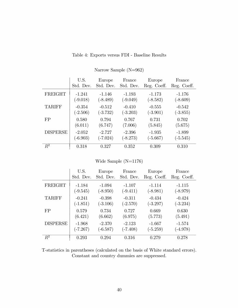
Table 4: Exports versus FDI - Baseline Results

Narrow Sample (N=962)

U.S. Europe France Europe FranceStd. Dev. Std. Dev. Std. Dev. Reg. Coeff. Reg. Coeff.

FREIGHT -1.241 -1.146 -1.193 -1.173 -1.176(-9.018) (-8.489) (-9.049) (-8.582) (-8.609)

TARIFF -0.354 -0.512 -0.410 -0.555 -0.542(-2.506) (-3.732) (-3.203) (-3.901) (-3.855)

FP 0.580 0.794 0.767 0.731 0.702(6.011) (6.747) (7.006) (5.845) (5.675)

DISPERSE -2.052 -2.727 -2.396 -1.935 -1.899(-6.903) (-7.024) (-8.273) (-5.667) (-5.545)

R2 0.318 0.327 0.352 0.309 0.310

Wide Sample (N=1176)

U.S. Europe France Europe FranceStd. Dev. Std. Dev. Std. Dev. Reg. Coeff. Reg. Coeff.

FREIGHT -1.184 -1.094 -1.107 -1.114 -1.115(-9.545) (-8.950) (-9.411) (-8.981) (-8.979)

TARIFF -0.241 -0.398 -0.311 -0.434 -0.424(-1.851) (-3.106) (-2.570) (-3.297) (-3.234)

FP 0.579 0.734 0.727 0.669 0.630(6.421) (6.662) (6.975) (5.773) (5.491)

DISPERSE -1.968 -2.370 -2.123 -1.667 -1.574(-7.267) (-6.587) (-7.408) (-5.259) (-4.978)

R2 0.293 0.294 0.316 0.279 0.278

T-statistics in parentheses (calculated on the basis of White standard errors).Constant and country dummies are suppressed.

40

Table 5: “Beta” Coefficients

Standard “Beta”Mean Deviation Coefficient

Dependent Var. -0.595 2.375

FREIGHT 1.863 0.653 -0.328

TARIFF 2.015 1.020 -0.204

FP 3.321 0.785 0.236

U.S. S.D. 1.749 0.316 -0.273Europe S.D. 1.198 0.276 -0.317France S.D. 1.224 0.375 -0.378Europe Reg. 1.260 0.333 -0.271France Reg. 1.257 0.336 -0.269

41

Table 6: Exports Versus FDI - Controls

Narrow Sample (N=961)

U.S. Europe France Europe FranceStd. Dev. Std. Dev. Std. Dev. Reg. Coeff. Reg. Coeff.

FREIGHT -1.040 -0.959 -1.019 -0.935 -0.944(-7.392) (-6.749) (-7.328) (-6.526) (-6.594)

TARIFF -0.365 -0.512 -0.421 -0.545 -0.539(-2.644) (-3.636) (-3.917) (-3.781) (-3.775)

FP 1.177 0.932 0.927 0.947 0.934(10.159) (7.827) (8.059) (7.453) (7.450)

DISPERSE -2.343 -2.153 -2.061 -1.503 -1.491(-8.374) (-5.250) (-6.664) (-4.535) (-4.470)

KL -0.868 -0.495 -0.456 -0.628 -0.626(-7.790) (-4.529) (-4.256) (-5.876) (-5.859)

RD -0.104 0.007 0.007 0.006 -0.002(-2.197) (0.150) (0.144) (0.125) (-0.047)

R2 0.373 0.340 0.364 0.332 0.334

Wide Sample (N=1175)

U.S. Europe France Europe FranceStd. Dev. Std. Dev. Std. Dev. Reg. Coeff. Reg. Coeff.

FREIGHT -1.011 -0.935 -0.960 -0.915 -0.919(-7.968) (-7.246) (-7.714) (-7.040) (-7.053)

TARIFF -0.241 -0.384 -0.306 -0.411 -0.407(-1.876) (-2.964) (-2.457) (-3.073) (-3.057)

FP 1.133 0.861 0.868 0.867 0.848(10.428) (7.719) (7.994) (7.318) (7.243)

DISPERSE -2.248 -1.866 -1.833 -1.284 -1.215(-8.611) (-4.919) (-5.982) (-4.132) (-3.924)

KL -0.793 -0.454 -0.412 -0.569 -0.576(-7.483) (-4.347) (-3.982) (-5.574) (-5.636)

RD -0.086 0.017 0.021 0.015 0.007(-1.914) (0.367) (0.446) (0.326) (0.153)

R2 0.338 0.305 0.325 0.298 0.298

T-statistics in parentheses (calculated on the basis of White standard errors).Constant and country dummies are suppressed.

42

Table 7: Exports versus FDI - Random Effects(With Controls)

Narrow Sample (N=961)

U.S. Europe France Europe FranceStd. Dev. Std. Dev. Std. Dev. Reg. Coeff. Reg. Coeff.

FREIGHT -0.430 -0.398 -0.428 -0.397 -0.397(-2.554) (-2.344) (-2.533) (-2.336) (-2.334)

TARIFF -0.113 -0.127 -0.105 -0.136 -0.133(-0.922) (-1.033) (-0.857) (-1.107) (-1.085)

FP 1.376 1.132 1.096 1.154 1.137(5.145) (4.128) (4.233) (4.107) (4.093)

DISPERSE -2.623 -2.763 -2.445 -2.031 -1.991(-4.897) (-3.459) (-4.761) (-3.098) (-3.180)

KL -1.106 -0.613 -0.570 -0.757 -0.758(-4.652) (-2.238) (-2.168) (-2.891) (-2.896)

RD -0.002 0.126 0.116 0.133 0.119(-0.020) (1.029) (0.970) (1.081) (0.972)

R2 0.352 0.316 0.342 0.307 0.308

Wide Sample (N=1175)

U.S. Europe France Europe FranceStd. Dev. Std. Dev. Std. Dev. Reg. Coeff. Reg. Coeff.

FREIGHT -0.331 -0.322 -0.328 -0.320 -0.320(-2.296) (-2.230) (-2.278) (-2.215) (-2.215)

TARIFF -0.004 -0.018 -0.004 -0.022 -0.021(-0.038) (-0.155) (-0.035) (-0.193) (-0.187)

FP 1.361 1.110 1.081 1.127 1.103(4.123) (3.455) (3.475) (3.377) (3.369)

DISPERSE -2.518 -2.559 -2.265 -1.864 -1.786(-3.824) (-2.733) (-3.706) (-2.398) (-2.424)

KL -1.069 -0.599 -0.561 -0.734 -0.739(-3.660) (-1.871) (-1.789) (-2.373) (-2.408)

RD 0.006 0.123 0.116 0.129 0.115(0.042) (0.862) (0.811) (0.894) (0.805)

R2 0.312 0.274 0.297 0.267 0.267

Z-statistics in parentheses. Constant and country dummies are suppressed.

43

Table 8: Exports versus FDI - Aggregated Europe(With Controls and Random Effects)

Wide Sample (N=680)

U.S. Europe France Europe FranceStd. Dev. Std. Dev. Std. Dev. Reg. Coeff. Reg. Coeff.

FREIGHT -0.493 -0.485 -0.487 -0.485 -0.483(-2.882) (-2.810) (-2.837) (-2.806) (-2.795)

TARIFF -0.005 -0.044 -0.032 -0.058 -0.052(-0.030) (-0.254) (-0.183) (-0.335) (-0.299)

FP 1.216 0.926 0.922 0.929 0.928(4.683) (3.713) (3.874) (3.620) (3.663)

DISPERSE -2.242 -1.845 -1.748 -1.301 -1.322(-4.351) (-2.595) (-3.765) (-2.217) (-2.371)

KL -0.989 -0.636 -0.588 -0.740 -0.737(-4.339) (-2.560) (-2.447) (-3.105) (-3.102)

RD -0.023 0.076 0.073 0.078 0.071(-0.208) (0.692) (0.671) (0.706) (0.648)

R2 0.314 0.273 0.289 0.268 0.270

Z-statistics in parentheses. Constant and country dummies are suppressed.

44

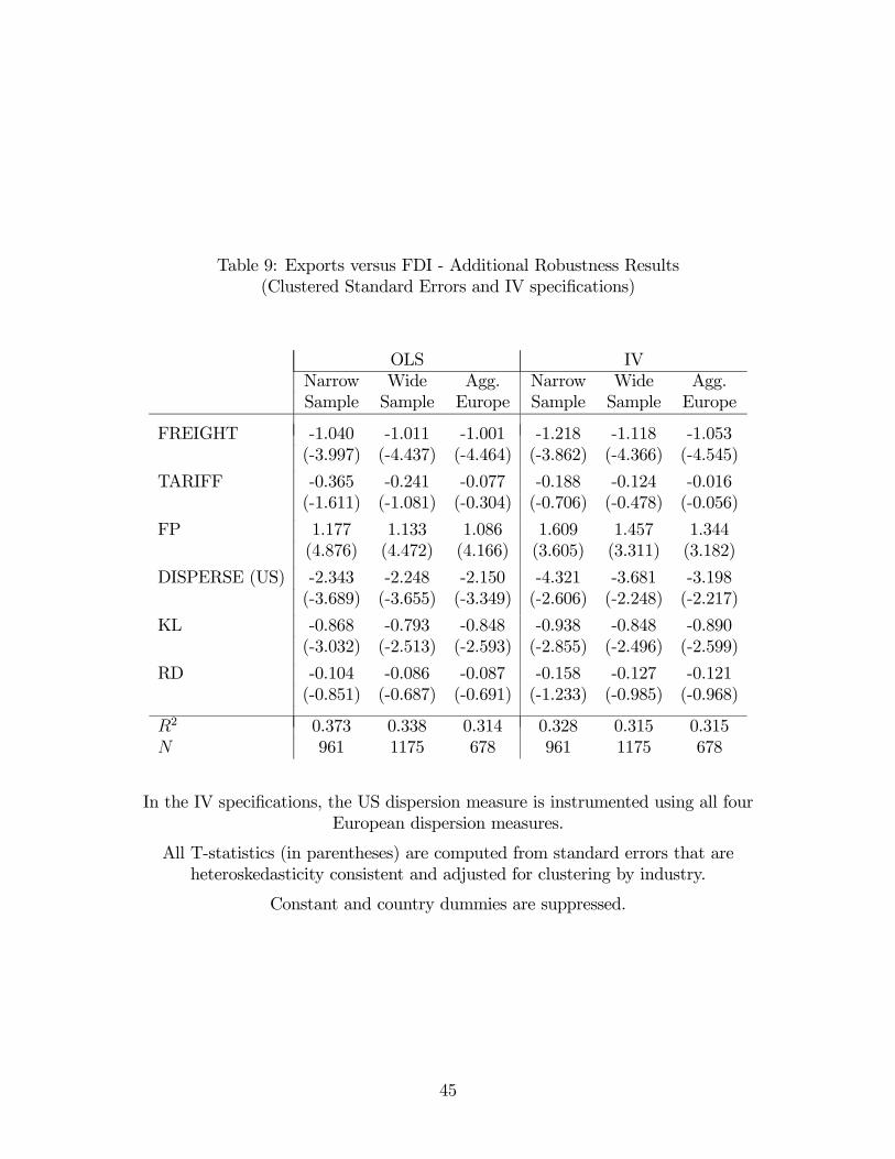
Table 9: Exports versus FDI - Additional Robustness Results(Clustered Standard Errors and IV specifications)

OLS IVNarrow Wide Agg. Narrow Wide Agg.Sample Sample Europe Sample Sample Europe

FREIGHT -1.040 -1.011 -1.001 -1.218 -1.118 -1.053(-3.997) (-4.437) (-4.464) (-3.862) (-4.366) (-4.545)

TARIFF -0.365 -0.241 -0.077 -0.188 -0.124 -0.016(-1.611) (-1.081) (-0.304) (-0.706) (-0.478) (-0.056)

FP 1.177 1.133 1.086 1.609 1.457 1.344(4.876) (4.472) (4.166) (3.605) (3.311) (3.182)

DISPERSE (US) -2.343 -2.248 -2.150 -4.321 -3.681 -3.198(-3.689) (-3.655) (-3.349) (-2.606) (-2.248) (-2.217)

KL -0.868 -0.793 -0.848 -0.938 -0.848 -0.890(-3.032) (-2.513) (-2.593) (-2.855) (-2.496) (-2.599)

RD -0.104 -0.086 -0.087 -0.158 -0.127 -0.121(-0.851) (-0.687) (-0.691) (-1.233) (-0.985) (-0.968)

R2 0.373 0.338 0.314 0.328 0.315 0.315N 961 1175 678 961 1175 678

In the IV specifications, the US dispersion measure is instrumented using all fourEuropean dispersion measures.

All T-statistics (in parentheses) are computed from standard errors that areheteroskedasticity consistent and adjusted for clustering by industry.

Constant and country dummies are suppressed.

45

Table A1: Dispersion Measures

Standard Deviation Reg. Coef. Standard Deviation Reg. Coef.Sector U.S. Eur. Fra. Eur. Fra. Sector U.S. Eur. Fra. Eur. Fra.201 2.15 1.16 1.13 1.18 1.19 329 1.48 0.90 0.89 0.94 0.95202 1.82 1.43 1.49 1.47 1.45 331 1.88 1.52 1.45 1.56 1.58203 2.03 1.12 1.17 1.14 1.12 335 1.49 1.34 1.20 1.40 1.38204 1.36 1.17 1.19 1.19 1.20 341 1.92 1.05 1.21 1.09 1.06205 1.96 1.11 1.06 1.15 1.18 342 1.71 0.86 0.81 0.88 0.90208 1.94 1.29 1.33 1.32 1.32 343 1.84 1.09 1.27 1.16 1.14209 1.69 1.16 1.12 1.19 1.21 349 1.62 1.03 0.92 1.05 1.03210 2.55 2.00 2.97 2.24 2.33 351 2.56 1.08 1.05 1.12 1.11220 1.84 0.96 0.99 0.97 0.96 352 1.81 1.20 1.07 1.28 1.30230 1.57 0.89 0.91 0.89 0.90 353 1.67 1.11 1.07 1.12 1.11240 1.53 0.90 0.81 0.91 0.92 354 1.40 1.11 1.04 1.13 1.14250 1.72 0.89 0.94 0.90 0.89 355 1.61 1.08 0.99 1.09 1.09262 1.25 1.19 1.07 1.27 1.27 356 1.66 1.05 1.15 1.06 1.08265 1.30 0.86 1.05 0.88 0.85 357 2.00 1.64 1.46 1.69 1.73271 1.66 1.22 1.26 1.28 1.28 358 1.85 1.04 0.99 1.05 1.05272 1.42 1.19 1.00 1.22 1.29 359 1.32 1.06 1.11 1.09 1.07275 1.34 0.55 0.52 0.55 0.54 363 2.45 1.55 1.55 1.62 1.65281 1.31 1.32 1.45 1.38 1.33 366 2.02 1.59 1.60 1.65 1.66283 2.11 1.62 1.55 1.68 1.77 367 1.91 1.18 1.27 1.22 1.20284 1.87 1.41 1.45 1.45 1.43 369 1.91 1.49 1.54 1.65 1.83287 1.64 1.59 1.58 1.66 1.65 371 2.16 1.71 1.78 1.74 1.76289 1.40 1.43 1.47 1.48 1.43 379 1.70 1.39 1.45 1.65 1.57305 1.62 0.73 0.71 0.75 0.75 381 2.33 1.50 1.88 2.16 2.00308 1.56 0.99 0.99 1.01 1.01 384 1.74 1.17 1.11 1.21 1.22310 1.73 0.84 0.88 0.84 0.85 386 1.79 1.34 1.75 1.66 1.37321 1.24 1.25 0.96 1.30 1.30 390 1.50 0.97 0.97 0.98 0.99

46