NBER WORKING PAPER SERIES

TWO FLAWS IN BUSINESS CYCLE ACCOUNTING

Lawrence J. ChristianoJoshua M. Davis

Working Paper 12647http://www.nber.org/papers/w12647

NATIONAL BUREAU OF ECONOMIC RESEARCH1050 Massachusetts Avenue

Cambridge, MA 02138October 2006

We are grateful for several key discussions with Mark Gertler, as well as for discussions with MartinEichenbaum. The views expressed herein are those of the author(s) and do not necessarily reflect theviews of the National Bureau of Economic Research.

© 2006 by Lawrence J. Christiano and Joshua M. Davis. All rights reserved. Short sections of text,not to exceed two paragraphs, may be quoted without explicit permission provided that full credit,including © notice, is given to the source.

Two Flaws In Business Cycle AccountingLawrence J. Christiano and Joshua M. DavisNBER Working Paper No. 12647October 2006JEL No. C01,C32,C52

ABSTRACT

Using 'business cycle accounting' (BCA), Chari, Kehoe and McGrattan (2006) (CKM) conclude thatmodels of financial frictions which create a wedge in the intertemporal Euler equation are not promisingavenues for modeling business cycle dynamics. There are two reasons that this conclusion is not warranted.First, small changes in the implementation of BCA overturn CKM's conclusions. Second, one waythat shocks to the intertemporal wedge impact on the economy is by their spillover effects onto otherwedges. This potentially important mechanism for the transmission of intertemporal wedge shocksis not identified under BCA. CKM potentially understate the importance of these shocks by adoptingthe extreme position that spillover effects are zero.

Lawrence J. ChristianoDepartment of EconomicsNorthwestern University2003 Sheridan RoadEvanston, IL 60208and NBERl-christiano@northwestern.edu

Joshua M. DavisDepartment of EconomicsNorthwestern UniversityEvanston, Illinois 60208j-davis7@northwestern.edu

1. Introduction

Chari, Kehoe and McGrattan (2005) (CKM) argue that a procedure they call Business CycleAccounting (BCA) is useful for identifying promising directions for model development.1 Thekey substantive finding of CKM is that financial frictions like those analyzed by Carlstromand Fuerst (1997) (CF) and Bernanke, Gertler and Gilchrist (1999) (BGG) are not promisingavenues for studying business cycles. Based on our analysis of business cycle data for theUS in the 1930s and for the US and 14 other OECD countries in the postwar period, we findthat the CKM conclusion is not warranted.The BCA strategy begins with the standard real business cycle (RBC) model, augmented

by introducing four shocks, or ‘wedges’. A vector autoregressive representation (VAR) forthe wedges is estimated using macroeconomic data on output, consumption, investmentand government consumption.2 The macroeconomic data are assumed to be observed with asmall measurement error whose variance is fixed a priori. The fitted wedges have the propertythat when they are fed simultaneously to the augmented RBC model, the model reproducesthe four macroeconomic data series up to the small measurement error. The importance ofa particular wedge is determined by feeding it to the model, holding all the other wedgesconstant, and comparing the resulting model predictions with the data. One of the wedges,the intertemporal wedge, is the shock that enters between the intertemporal marginal rate ofsubstitution in consumption and the rate of return on capital. CKM argue that this wedgecontributes very little to business cycle fluctuations, for the following two reasons: (i) thewedge accounts for only a small part of the movement in macroeconomic variables duringrecessions and (ii) the wedge drives consumption and investment in opposite directions,while these two variables display substantial positive comovement over the business cycle.CKM assert that their conclusions are robust to various model perturbations, including theintroduction of adjustment costs in investment.There are two reasons that BCA does not warrant being pessimistic about the useful-

ness of models of financial frictions such as those proposed in CF or BGG. First, CKM’sconclusions are not robust to small changes in the way they implement BCA. For example,when we redo CKM’s calculations for the 1982 recession, we reproduce their finding that theintertemporal wedge accounts for essentially no part of the decline in output below trendat the trough of the recession. When we introduce a modest amount of investment adjust-ment costs, the intertemporal wedge accounts for a substantial 34 percent of the drop inoutput at the trough of the recession.3 We then consider an alternative specification of theintertemporal wedge which is at least as plausible as the one CKM work with. CKM definethe intertemporal wedge as an ad valorem tax on the price of investment goods. We arguethat the CF and BGG models motivate considering an alternative formulation in which the

1This strategy is closely related to that advocated in Parkin (1988), Ingram, Kocherlakota and Savin(1994), Hall (1997), and Mulligan (2002).

2The last variable includes government consumption and net exports.3Our adjustment costs are ‘modest’ in two senses. First, they imply a steady state elasticity of the

investment-capital ratio to the price of capital equal to unity. This lies in the middle of the range ofempirical estimates reported in the literature. Second, the adjustment cost function has the property thatthe quantity of resources lost due to investment adjustment costs is small, even in the wake of the enormousdecline in investment in the early 1930s (see section 4 below for a detailed discussion).

2

wedge is modeled as a tax on the gross rate of return on capital. When we work with this al-ternative formulation, the intertemporal wedge accounts for 26 percent of the drop in outputat the trough of the 1982 recession. But, when we also drop CKM’s model of measurementerror, that quantity jumps to 52 percent. Notably, the CKM model of measurement error isoverwhelmingly rejected in the post war US data. So, BCA actually places a range of 0 to52 percent on the fraction of the drop in output accounted for by the intertemporal wedge inthe 1982 recession. This range is sufficiently wide to comfortably include most views aboutthe importance of the intertemporal wedge.We show that, at a qualitative level, economic theory predicts the lack of robustness in

BCA that we find. The intertemporal wedge associated with different perturbations of theRBC model represent different ways of bundling the fundamental economic shocks to theeconomy. As a result, the BCA experiment of feeding measured wedges to an RBC modelrepresents fundamentally different economic experiments under alternative specifications ofthe RBC model. Since the experiments are different, the outcomes are expected to bedifferent too. Our results show that these expected differences are quantitatively large enoughto overturn CKM’s conclusions.Second, CKM’s analysis ignores that the financial shocks which drive the intertemporal

wedge may have spillover effects onto other wedges.4 It is not possible to determine themagnitude of these effects with BCA, because BCA leaves the fundamental shocks to theeconomy unidentified. In fact, the VAR for the wedges estimated under BCA is consistentwith a wide range of possible spillover patterns. In terms of CKM’s conclusion (i) above,we show that the financial shocks which drive the intertemporal wedge could account foras much as 70-100 percent of reductions in output in US recessions, including the GreatDepression. We obtain the same finding for several other countries in the OECD. RegardingCKM’s conclusion (ii), we show that once spillover effects are taken into account, financialshocks which drive the intertemporal wedge can drive consumption and investment in thesame direction.CKM understand that the fundamental economic shocks are not identified under BCA.

However, the implications they draw from this observation are very different from the oneswe draw. They say, ‘Our method is not intended to identify the primitive sources of shocks.Rather, it is intended to help understand the mechanisms through which such shocks lead toeconomic fluctuations.’5 We find that, without the ability to identify the economic shocks,a potentially important part of the mechanism by which these shocks affect the economy -the spillover effects - is also not identified. In effect, BCA offers a menu of observationallyequivalent assessments about the importance of shocks to the intertemporal wedge. Byfocusing exclusively on the extreme case of zero spillovers, CKM select the element in themenu which minimizes the role of intertemporal shocks. We show that there are otherelements in that menu which assign a very large role to intertemporal shocks.

4Recent developments in economic modeling suggest a variety of mechanisms by which these spillovereffects can occur. For example, it is known that in models with Calvo-style wage-setting frictions (see,e.g., Erceg, Henderson and Levin (2000)), a shock outside the labor market can trigger what looks like apreference shock for labor, or a ‘labor wedge’. Similarly, variable capital utilization can have the effect thata non-technology shock triggers a move in measured TFP, or the ‘efficiency wedge’.

5The quote is taken from the CKM introduction. It summarizes CKM’s comments in section 3 of theirpaper.

3

Following is an outline of the paper. In the following section, we describe the model usedin the analysis. In section 3, we elaborate on the observational equivalence results discussedabove. In section 4, we discuss our model solution and estimation strategy. In section 5 wediscuss the lack of identification of spillover effects in BCA. In section 6 we discuss the wedgedecomposition under BCA and our modification to take into account spillovers. Section 7displays the results of implementing BCA on various data sets. Concluding remarks appearin section 8. Additional technical details appear in three Appendices.

2. The Model and the Wedges

This section describes the model used in the analysis. In addition, we discuss the wedgesand, in particular, our two specifications of the intertemporal wedge.According CKM’s version of the RBC model, households maximize:

E∞Xt=0

(β (1 + gn))t [log ct + ψ log (1− lt)] , 0 < β < 1,

where ct and lt denote per capita consumption and employment, respectively. Also, gn is thepopulation growth rate and ψ > 0 is a parameter. The household budget constraint is

ct + (1 + τx,t)xt ≤ rtkt + (1− τ l,t)wtlt + Tt,

where Tt denotes lump sum taxes, xt denotes investment and τ l,t denotes the labor wedge.Here, kt denotes the beginning-of-period t stock of capital divided by the period t population.The variable, τx,t, is CKM’s specification of the intertemporal wedge. The technology forcapital accumulation is given by:

(1 + gn) kt+1 = (1− δ) kt + xt − Φ

µxtkt

¶kt, (2.1)

where Φ (ζ) is symmetric about ζ = b, where b is the steady state investment-capital ratio. Inaddition, to ensure that Φ has no impact on steady state, we suppose that Φ (b) = Φ0 (b) = 0.The household maximizes utility by choice of {ct, kt+1, lt, xt} , subject to its budget con-

straint, the capital evolution equation, the laws of motion of the wedges and the usualinequality constraints and no-Ponzi scheme condition.The resource constraint is:

ct + gt + xt = y (kt, lt, Zt) = kαt (Ztlt)1−α , (2.2)

whereZt = Zt (1 + gz)

t ,

and Zt, the ‘efficiency’ wedge, is an exogenous stationary stochastic process. In the resourceconstraint, gt denotes government purchases of goods and services plus net exports, whichis assumed to have the following trend property:

gt = gt (1 + gz)t ,

4

where gt is a stationary, exogenous stochastic process and gz ≥ 0.Combining firm and household first order necessary conditions for optimization in the

case Φ = 0,

−ul,tuc,t

= (1− τ l,t) yl,t (2.3)

uc,t = βEtuc,t+1yk,t+1 + (1 + τx,t+1)Pk0,t+1

h1− δ − Φ

³xt+1kt+1

´+ Φ0

³xt+1kt+1

´xt+1kt+1

i(1 + τx,t)Pk0,t

(2.4)

where uc,t and −ul,t are the derivatives of period utility with respect to consumptionand leisure, respectively. In addition, yl,t and yk,t are the marginal products of labor andcapital, respectively. Also, the price of capital, Pk0,t, is

Pk0,t =1

1− Φ0³xt+1kt+1

´ . (2.5)

The equilibrium values of {ct, kt+1, lt, xt} are computed by solving (2.1), (2.2), (2.3), (2.4),subject to the transversality condition and the following law of motion for the exogenousshocks:

st = [I − P ]P0 + Pst−1 + ut, st =

⎛⎜⎜⎝log Zt

τ l,tτx,tlog gt

⎞⎟⎟⎠ , Eutu0t = QQ0 = V, (2.6)

where P0 is the 4× 1 vector of unconditional means for st and

P =

∙P 00 p44

¸, Q =

∙Q 00 q44

¸. (2.7)

Here, P is stationary and P is not otherwise restricted. The symmetric matrix, V, in (2.6)must satisfy the zero restrictions implicit in QQ0 = V, and the zeros in the lower diagonalpart of Q in (2.7). We follow CKM in implementing the zero restrictions in our analysisof the US Great Depression. We do this in our analysis of OECD countries as well. Inour analysis of postwar US data, we allow all elements of P and all elements in the lowertriangular part of Q to be non-zero. The parameters of (2.6) are P0, P, and V, possibly withthe indicated zero restrictions on V and the zero and stationarity restrictions on P.We consider an alternative specification of the intertemporal wedge. Our specification is

motivated by our analysis of the version of the CF model with adjustment costs and by ouranalysis of BGG. In Appendix A, we derive equilibrium conditions for a version of the CFmodel with Φ 6= 0. We establish a proposition displaying a set of wedges which, if addedto the RBC economy, ensure that the equilibrium allocations of the RBC economy coincidewith those of our version of the CF economy with investment adjustment costs. We showthat the intertemporal wedge has the following form:

uc,t = βEtuc,t+1¡1− τkt+1

¢Rkt+1, (2.8)

5

where,

Rkt =

yk,t + Pk0,t

h1− δ − Φ

³xtkt

´+ Φ0

³xtkt

´xtkt

iPk0,t−1

(2.9)

Note that in the alternative formulation, the wedge is a tax on the gross return to capital, incontrast to CKM’s value-added tax on investment purchases, τx,t. In Appendix A we showthat the CF model with adjustment costs implies τkt+1 is a function of uncertainty realizedat date t, but not at date t+ 1.6 We follow CKM in presuming that all wedges implied bythe CF financial frictions apart from the intertemporal wedge, 1 − τkt+1, are quantitativelysmall and can be ignored.In Appendix B we derive the intertemporal wedge associated with the BGG model. That

model also implies that the intertemporal wedge enters as 1−τkt+1 in (2.8). The only differenceis that under BGG, τkt+1 is a function of the period t+ 1 realization of uncertainty.7

In our alternative specification of the intertemporal wedge, we allow τkt to respond tocurrent and past information. This assumption encompasses both the CF and BGG financialfriction models, since the econometric estimation is free to produce a τkt whose response tocurrent information is very small.

3. General Observations on the Robustness of BCA to ModelingDetails

In later sections, we show that the conclusions of BCA for the importance of the intertem-poral wedge are not robust to alternative specifications of the intertemporal wedge, and toalternative specifications of investment adjustment costs. This finding may at first seem puz-zling in light of a type of observational equivalence result emphasized in CKM. An exampleof this type of result which occurs when BCA is done with a linearly approximated RBCmodel is the following. Consider an RBC economy with, say, no investment adjustment costs(i.e., Φ = 0) and a particular time series representation for the wedges. After introducingadjustment costs (i.e., Φ 6= 0), one can find a new representation of the intertemporal wedgewhich ensures that the equilibria of the economies with and without adjustment costs coin-cide.8 This is an observational equivalence result because it implies that the likelihood of a

6That appendix provides a careful derivation of our result, because our finding for the way the intertem-poral wedge enters (2.8) differs from CKM’s finding. CKM consider the case, Φ = 0, in deriving the wedgerepresentation of the CF model. The results for the Φ = 0 and Φ 6= 0 cases are qualitatively different.When Φ = 0 capital producers simply produce increments to the capital stock, which capital owners addto the existing undepreciated capital by themselves. When Φ 6= 0, old capital is a fundamental input inthe production of new capital. In this case, we assume that the capital producers must purchase the econ-omy’s entire stock of capital in order to produce new capital, so that their financing requirements and theassociated frictions are different. There are perhaps other ways of arranging the production of new installedcapital when Φ 6= 0. We find our way convenient because it results in an intertemporal wedge that virtuallycoincides with the one we derive for BGG

7CKM derive the intertemporal wedge for a version of the BGG model in which banks have access tocomplete state-contingent markets. Our wedge formula applies to the model analyzed in BGG, which doesnot permit complete markets.

8Here, we make use of our asumption that analysis is done using log-linear approximation. In this case,the only effect of the change in Φ is to change the rate of return on capital. For example, in the linear

6

set of allocations is invariant to the presence of adjustment costs. This case of adjustmentcosts is just example of the type of observational equivalence result we have in mind. Forexample, consider an RBC economy in which the intertemporal wedge is of the τx,t typeemphasized by CKM. Given a specification of the joint time series representation of τx,t andthe other wedges, the τx,t RBC model implies a set of equilibrium allocations. Now consideran alternative RBC economy in which the intertemporal wedge is of the τkt type. Thereexists a specification of the joint stochastic process for τkt and the other wedges having theproperty that the equilibrium allocations in the τkt RBCmodel coincide with those in the τx,tRBC model. Again, this stochastic process is identified from the requirement that the aftertax rates of return in the two economies coincide. In both of the above examples, it is clearthat the observational equivalence result depends on the assumption that the time seriesrepresentations used for the shocks are sufficiently flexible to accommodate any specificationfor the stochastic process of the wedges.9

We wish to stress here that the equilibrium observational equivalence result does notimply a ‘BCA robustness result’. In particular, the outcome of BCA (i.e., the outcome offeeding fitted wedges, one at a time, to a model) is not expected to be robust to the specifi-cation of investment adjustment costs, or to whether the intertemporal wedge is modeled asτx,t or τkt . There are two reasons for this lack of robustness. One is practical and reflects thatthe analyst must confine him/herself to a specific parametric time series representation ofthe wedges, thus potentially ruling out one of the conditions of the observational equivalenceresult. The other, deeper, reason is the one mentioned in the introduction. Even if theanalyst uses a completely flexible time series representation of the wedges, the intertemporalwedge represents a different bundle of fundamental shocks under alternative perturbationsof the model. Feeding the measured intertemporal wedge to an RBC model under alterna-tive model perturbations represents a different experiment and so is expected to produce adifferent outcome.To illustrate these observations, suppose the data are generated by an RBC model in

which intertemporal wedge is the τkt type, with a certain specification of the adjustment costfunction, Φ. The joint time series representation of the wedges is given by (2.6), in which Pand Q are diagonal. Thus, each wedge is uncorrelated with all other wedges, at all leads andlags. In this case, BCA has a clear interpretation: when the estimated intertemporal wedgeis fed to the baseline RBCmodel, the simulations display the model’s response to a particularhistory of past innovations to that wedge alone. Suppose the econometrician is provided withan infinite amount of data, but misspecifies the adjustment cost function, Φ. As in BCA,the econometrician only estimates the joint time series representation of the wedges, andholds the misspecified Φ and other nonstochastic parts of the economy fixed. We assumethat the econometrician’s time series representation for the wedges is sufficiently flexibleto encompass the quasi-true time series of the wedges that is implied by the observationalequivalence result. We obtain insight into BCA by deriving that time series representation.The requirement that the after tax rates of return in the econometrician’s model coincide

approximation the law of motion for the capital stock, (2.1), is always linear and invariant to a.9This is a special case of a well-known result that econometric identification often hinges on having

sufficient restrictions on the unobserved shocks.

7

with the true after tax rate of return implies, using (2.9):

1− τkt+1 =¡1− τkt+1

¢ yk,t + Pk0,t

h1− δ − Φ

³xtkt

´+ Φ0

³xtkt

´xtkt

iyk,t + Pk0,t

h1− δ − Φ

³xtkt

´+ Φ0

³xtkt

´xtkt

i . (3.1)

Here, a − over a variable indicates the value of the variable in the true model and absence ofa − indicates the value estimated by the econometrician who misspecifies Φ. The endogenousvariables on the right side of the equality in (3.1) are specific functions of the history of theinnovations driving the wedges in the actual economy. Then, according to (3.1), the adjustedtime series representation of τkt is the convolution of these functions with the function onthe right of the equality in (3.1). We derive this map from the fundamental innovations inthe economy to τkt using linearization.Consider the true specification of Φ and the true joint time series representation of the

wedges, st, given in (2.6). Let zt denote the list of endogenous variables in the model, i.e.,zt = (ct, xt, kt+1, lt, τ

kt ), where the quantity variables are measured in log deviations from

steady state and τkt is in deviation from steady state. The equilibrium conditions of zt maybe written in the form:

Et [α0zt+1 + α1zt + α2zt−1 + β0st+1 + β1st] = 0, with st = Pst−1 +Qεt.

Here, st =³log Zt, τ l,t, τ

kt , log gt

´0. The expectational difference equation is composed of

the intertemporal first order condition (2.8), the intratemporal first order condition (2.3),the law of motion for capital (2.1), the resource constraint, (2.2), and the mapping fromτkt to τkt , (3.1), all after suitable log-linearization. The solution to this system is writtenzt = Azt−1 +Bst, or, when expressed in moving average form10:

zt = [I −AL]−1B [I − PL]−1Qεt.

Let τ denote the 5-dimensional column vector with all zeros, except a 1 in the 5th location.Then, the time series representation for τkt is

τkt = τ [I −AL]−1B [I − PL]−1Qεt.

This is the convolution of (3.1) with the time series representation of the (linearized) vari-ables in (3.1). Let ν denote the 3 by 4 matrix constructed by deleting the third row ofthe 4-dimensional identity matrix and let St denote the 3 dimensional vector obtained bydeleting τkt from st. We conclude that the econometrician who misspecifies Φ will estimatethe following joint time series representation for the wedges in his misspecified model:µ

τktSt

¶=

∙τ [I −AL]−1B

ν

¸[I − PL]−1Qεt.

By inspection, it is clear that in general, the new joint series representation of¡τkt , St

¢has

a moving average component. To see this, it is useful to examine the iid case, P = 0 and

10For further discussion, see Christiano (2002).

8

Q = I. Note first that τ [I −A]−1B has the following form:

τ [I −A]−1B = τ

⎡⎢⎢⎢⎢⎢⎢⎣1 0 −a13L 0 0 00 1 −a23L 0 0 00 0 1− a33L 0 0 00 0 −a43L 1 0 00 0 −a53L 0 1 00 0 −a63L 0 0 1

⎤⎥⎥⎥⎥⎥⎥⎦

−1

B = τ

⎡⎢⎢⎢⎢⎢⎢⎢⎣

1 0 −L a13La33−1 0 0 0

0 1 −L a23La33−1 0 0 0

0 0 − 1La33−1 0 0 0

0 0 −L a43La33−1 1 0 0

0 0 −L a53La33−1 0 1 0

0 0 −L a63La33−1 0 0 1

⎤⎥⎥⎥⎥⎥⎥⎥⎦B

=£0 0 −a63L 0 0 1

¤B

=£B51 − a63B31L B52 − a63B32L B53 − a63B33L B54 − a63B34L

¤,

where Bij denotes the ijth element of B. We conclude that the new joint representation ofthe wedges is:µ

τktSt

¶=

∙ ¡B51 − a63B31L B52 − a63B32L B53 − a63B33L B54 − a63B34L

¢ν

¸εt.

Note that the intertemporal wedge has a pure, first order moving average representation,even though τkt in the correctly specified economy is iid and a function only of the thirdelement of εt. Evidently, the wedges in the misspecified economy do not obey the same firstorder VAR(1) representation that st does. Thus, the analyst who is restricted VAR(1) (or,VAR(q), q <∞) representations for the wedges misrepresents the reduced form of the data.Under these circumstances, it is not surprising that the conclusions of BCA will be different,across different specifications of Φ.Now, suppose that the analyst adopts a sufficiently flexible time series representation

of the wedges, so that the specification error described in the previous paragraph does notoccur. The intertemporal wedge, τkt , computed by the econometrician working with thecorrect specification of Φ is a function of just the current realization of the third element ofεt. In the alternative specification, τkt is a function of the entire history of all elements of εt.Clearly, feeding the estimated intertemporal wedge to the model is a different experimentacross the two different specifications of Φ. This is why we do not expect the results of BCAto be robust to perturbations in the RBC model.

4. Model Solution and Estimation

Here, we describe how we assigned values to the model parameters. A subset of the para-meters were not estimated. These were set as in CKM:

β = 1/1.03, α = 0.35, δ = 0.0464, ψ = 2.24, (4.1)

gn = 0.015, gz = 0.016.

Here, β, δ, gn, and gz are expressed at annual rates. These are suitably adjusted when weanalyze quarterly data. The first subsection below discusses the estimation of the parametersof the exogenous shocks, P0, P, and V, using data on output, consumption, investment and

9

government consumption plus net exports. Estimation is carried out conditional on a para-meterization of the adjustment cost function. The parameterization of the adjustment costfunction is discussed in the second subsection. The third subsection rebuts some criticismsof the investment adjustment cost function expressed in CKM. Their criticisms suggest thatinvestment adjustment costs are, in effect, a ‘nonstarter’. Since they are not empirically in-teresting, they therefore do not constitute a compelling basis for criticizing BCA. We explainwhy we disagree with this assessment.

4.1. Estimating the Parameters of the Time Series Representation of the Wedges

For the US Great Depression, we used annual data covering the period, 1901-1940.11 Quar-terly data covering the period 1959Q1-2004Q3 were used for the US and quarterly data overvarious periods were used on 14 other OECD countries.12 Following CKM, the elements ofthe matrices, P and V are estimated subject to the zero restrictions described in section 2,and to the restriction that the maximal eigenvalue of P not exceed 0.995.The first step of estimation is to set up the model’s solution in state space - observer

form:

Yt = H (ξt; γ) + υt (4.2)

ξt = F¡ξt−1; γ

¢+ ηut (4.3)

γ = (P, P0, V ) , η =

µ0I

¶, Eυtυ

0t = R, Eutu

0t = V,

where 0 is a 1× 4 vector of zeros and ξt is the state of the system:

ξt =

µlog ktst

¶, (4.4)

where kt = kt/ (1 + gz)t. Also, Yt is the observation vector:

Yt =

⎛⎜⎜⎝log ytlog xtlog ltlog gt

⎞⎟⎟⎠ , (4.5)

where xt = xt/ (1 + gz)t . Finally, υt is a 4× 1 vector of measurement errors, with

R = 0.0001× I4, (4.6)

where I4 is the four-dimensional identity matrix and CKM set the scale factor exogenously(see CKM (technical appendix, page 16)). We refer to this specification of R as the ‘CKM

11These data were taken from CKM, as supplied on Ellen McGrattan’s web site.12US data are the data associated with the CKM project, and were taken from Ellen McGrattan’s web

page. With two exceptions, data for other OECD countries were taken from Chari, Kehoe and McGrattan(2002), also on Ellen McGrattan’s web site. Data on hours worked were taken from the OECD productivitydatabase. These data are annual and were converted to quarterly by log-linear interpolation. Populationdata were taken from the OECD national databases and log-linearly intertpolated to quarterly.

10

measurement error assumption’. We repeat the analysis under CKM measurement error, aswell as with R = 0.As noted in the introduction, the CKM specification of measurement error has an impact

on the analysis. CKM do not explain why they include measurement error, nor do theydiscuss the a priori evidence which leads them to the specific values they choose for themeasurement error variance.13 We do have reason to believe the data are measured witherror. However, we know of no reason to take seriously the notion that CKM’s specificationeven approximately captures actual data measurement error.14

We implement BCA using first and second-order approximations to the model’s equilib-rium conditions. Consider the first order approximation. In this case, the representation ofthe policy rule is:

log kt+1 = (1− λ)λ0 + λ log kt + ψst, (4.7)

where λ0 and λ are scalars and ψ is a 1× 4 row vector. Then, (4.2)-(4.3) can be written:

ξt = F0 + F1ξt−1 + ηεt,

F0 =

∙(1− λ)λ0(I − P )P0

¸, F1 =

∙λ ψ0 P

¸,

where F0 is a 5× 1 column vector, and F1 is a 5× 5 matrix. Also,

Yt = H0 +H1ξt + υt, (4.8)

where H0 is a 4 × 1 column vector and H1 is a 4 × 4 matrix. The Gaussian likelihood isconstructed using F0, F1, H0, H1, V, R, and Y = (Y1, ..., YT ) (see Hamilton (1994)). Thesein turn can be constructed using γ, R. Thus, the likelihood can be expressed as L (Y |γ;R) .For the nonlinear case, we use the algorithm in Schmitt-Grohe and Uribe (2004) to obtain

second order approximations to the functions, F and H in (4.2) and (4.3). It is easy to seethat even if ut is Normally distributed, Yt will not be Normal in this nonlinear system.We nevertheless proceed to form the Gaussian density function using the unscented filterdescribed in Wan and van der Merwe (2001). It is known that under certain conditions,Gaussian maximum likelihood estimation has the usual desirable properties, even when thedata are not Gaussian.

4.2. Investment Adjustment Costs

To analyze the version of the model with adjustment costs, we must parameterize the in-vestment adjustment cost function, Φ. Our calibration is based on our interpretation of thevariable, Pk0,t. On this dimension, the CF and BGG models differ slightly (for details, seeAppendices A and B). Both agree that Pk0,t is the marginal cost, in units of consumption

13As already noted, other parameter values are also fixed in the analysis, such as production functionparameters. Dogmatic priors like this can perhaps be justified by appealing to analyses based on other data,such as observations on income shares. We are not aware of any such argument, however, that can be usedas a basis for adopting the dogmatic priors in (4.6).14Based on what we know about the way data are collected, there is strong a priori reason to question the

CKM model of measurement error. For a careful discussion, see Sargent (1989).

11

goods, of producing new capital when only (2.1) is considered.15 However, in the CF model,financial frictions introduce a wedge between the market price of capital and Pk0,t. Still, inpractice the discrepancy between Pk0,t and the market price of new capital in the CF modelwith adjustment costs may be quantitatively small. To see this, it is instructive to considerthe response of the variables in the CF model (where Pk0,t = 1 always) to a technology shock.According to CF (see Figure 2 in CF), the contemporaneous response of the market priceof capital is only one-tenth the contemporaneous response of investment. That simulationsuggests that the distinction between Pk0,t and the market price of capital may not be largein the CF model.In the BGG model, financial frictions arise inside the relationship between the managers

of capital and banks, and so the frictions do not open wedge between the marginal cost ofcapital and Pk0,t. As a consequence, Pk0,t corresponds to the market price of capital in theBGG model.Under the interpretation of Pk0,t as the market price of capital, we can calibrate Φ based

on empirical estimates of the elasticity of investment with respect to the price of capital (i.e.,Tobin’s q). From (2.5), this is

d log (xt/kt)

d logPk0,t=

1

Φ00 (b) b. (4.9)

According to estimates reported in Abel (1980) and Eberly (1997), Tobin’s q lies in a rangeof 0.6 to 1.4. Interestingly, if we just consider the period of largest fall in the Dow JonesIndustrial average during the Great Depression, 1929Q4 to 1932Q4, the ratio of the percentchange in investment to the percent change in the Dow is 0.68.16 This is an estimate ofTobin’s q under the assumption that the movement in the Dow reflects primarily the priceof capital, and not its quantity.17 This estimate lies in the middle of the Abel-Eberly rangeof estimates. A unit Tobin’s q elasticity implies Φ00 (b) = 1/b.Another factor impacting on our choice of Φ00 (b) is the model’s implication for the rate

of return on capital, Rk. Figure 1A shows the results corresponding to Tobin’s q elasticities1/2, 1, 3 and ∞ (the latter corresponds to Φ00 (b) = 0). For each elasticity, the modelwas estimated using the linearization strategy and using quarterly US data covering theperiod 1959QIV-2003QI. For these calculations, the only feature of Φ that is required is thevalue of Φ00 (b) . The model-based estimate of Rk

t , (2.9), was computed using the two-sidedKalman smoother.18 The US data on Rk

t were constructed using Robert Shiller’s data onreal dividends and real stock prices for the S&P composite index. In the case of both model-based and actual Rk

t , we report centered, equally weighted, 5 quarter moving averages. Notethat without adjustment costs, the model drastically understates the volatility in Rk

t . With

15It is easy to verify that Pk0,t in (2.1) corresponds to the price of investment goods (i.e., unity) dividedby the marginal product of investment goods in producing end of period capital.16This is the ratio of the log difference in investment to the log difference in the Dow, over the period

indicated. Both variables were in nominal terms.17By associating the model’s capital stock with what is priced in the Dow, we are implicitly taking the

position that capital in the model corresponds to both tangible and intangible capital.18See Hamilton (1994) for a discussion. The two-sided smoother is required because we do not use empirical

data on the capital stock, which is an input in (2.9). Presumably, the smoother estimates the capital stockby combining the investment data with the capital accumulation equation.

12

a Tobin’s q elasticity of 3 (i.e., Φ00 (b) = 1/(3b)) the model still substantially understatesthat volatility. With an elasticity around unity, the model begins to reproduce the volatilityof Rk, though it is still somewhat low. Only with an elasticity around 1/2 does the modelnearly replicate the volatility of Rk. These results reinforce our impression that the datasuggest a Tobin’s q elasticity of unity or less. To be conservative, we work with an elasticityof unity.

4.3. Responding to CKM’s Criticisms About Adjustment Costs

CKM criticize the use of adjustment costs with a unit Tobin’s q elasticity for two reasons.According to their first critique, adjustment costs with a unit Tobin’s q elasticity implythat an unreasonably large amount of resources are absorbed by adjustment costs duringcollapse of investment in the Great Depression. This conclusion is based on the arbitraryassumption that the adjustment cost function, Φ, is globally quadratic. But, we show thatother functional forms for Φ can be found with the property, Φ00 (b) = 1/b, whose globalproperties do not imply that an inordinate amount of resources were used up in investmentadjustment costs in the Great Depression. Second, CKM assert that an adjustment costformulation which implies a static relationship between the investment-capital ratio andTobin’s q is empirically implausible. But, we show that BCA lacks robustness even withthe specification of adjustment costs proposed in Christiano, Eichenbaum and Evans (2004),which does not imply a static relationship the investment-capital ratio and Tobin’s q. Thisadjustment cost function, in which adjustment costs are a function of the change in the flowof investment, also does not imply that an inordinate amount of resources were used up inadjustment costs during the collapse of investment in the 1930s.19

The globally quadratic adjustment cost formulation adopted by CKM is:

Φ

µxtkt

¶=

a

2

µxtkt− b

¶2,

so that Φ00 (b) = a. Imposing that Tobin’s q elasticity is unity, the resources lost to adjustmentcosts, as a fraction of output, is given by:

Φ

µxtkt

¶=1

2(λt − 1)2

x

yµt, (4.10)

according to (2.1). Here, x/y is the steady state investment to output ratio. In (4.10),we have used x = bk in the steady state. Here, λt is the time t investment-capital ratio,expressed as a ratio to its steady state value, b. Also, µt is the output-capital ratio, expressedas a ratio to its steady state value, y/k. Figure 6 indicates that output was 10 percent belowtrend in 1930, and then fell another 10 percent in each of 1931 and 1932. In 1933, the troughof the Depression, it fell yet another 5 percent, so that by 1933 output was a full 35 percent

19This adjustment cost function has the additional advantage that it receives empirical support from theanalysis of housing investment (see Rosen and Topel (1988)) and aggregate Tobin’s q data (see Matsuyama(1984)), in addition to the empirical evidence in Christiano, Eichenbaum and Evans (2006). Also, thisadjustment cost formulation has economically interesting microfoundations, as shown in Lucca (2006) andMatsuyama (1984).

13

below trend. The drop in investment was even more dramatic. In 1930, 1931, 1932 and1933 it was about 30, 50, 70 and 70 percent below trend, respectively. Using our capitalaccumulation equation, we infer that the stock of capital was 10 percent below trend in 1933.Since investment was 70 percent below its trend in 1933 and the capital stock was 10

percent its trend then, we infer that the investment to capital ratio is 60 percent below steadystate, i.e., λ1933 = 0.40. Output was 35 percent below steady state in 1933, and we infer thatthe output-capital ratio was 25 percent below trend, so that µ1933 = 0.75. Substituting theseinto (4.10),

Φ

µxtkt

¶=1

2(0.40− 1)2 (0.23) /0.75 = 0.055,

or 5.5 percent. Given that output was 35 percent below trend in 1933, the implication is that16 percent of the drop in output reflected resources lost to adjustment costs associated withthe low level of investment. To see how sensitive this conclusion is to the choice of functionalform for Φ, consider Figure 1B, which graphs (4.10) for 100λt ranging from 40 percent to160 percent, holding x/ (yµt) fixed at 0.31. Note how the quadratic curve hits the verticalaxis at 5.5 percent. The other curve in Figure 1B coincides with the quadratic functionfor λt roughly in its range for postwar business cycles. Outside this range, the alternativefunction is flatter than the quadratic, and it hits the vertical axis at 2.5 percent. Thealternative adjustment cost function has a much more modest implication for the amountof resources lost to adjustment costs as investment collapsed in the Great Depression. Yet,the implications of the model with the alternative adjustment cost function for postwarbusiness cycles coincides with the implications of the model with the quadratic adjustmentcost function.20

To address CKM’s second concern about adjustment costs, we also considered the fol-lowing formulation:

(1 + gn) kt+1 = (1− δ) kt +

"1− a

2

µxtxt−1

− 1¶2#

xt.

With this formulation of adjustment costs, investment responds differently to permanentand temporary changes in the price of capital. This addresses one of CKM’s concerns aboutinvestment adjustment costs. To address the other concern, we needed to assign a value toa. For this, we estimated the parameters of the joint time series representation of the wedgesfor various values of a, using postwar US data. We found that with a = 3.75 the model’simplications for the volatility of the rate of return on capital virtually coincides with theimplications of our baseline model with a unit Tobin’s q elasticity. We then used the Balkeand Gordon quarterly data on investment and output in the 1930s to compute the fractionof output lost due to adjustment as investment plunged at the start of the Great Depression.We found that the largest fraction of output lost due to adjustment costs in the period1929Q1-1933Q1 was 1.46 percent. According to the Balke and Gordon data, investment

20The alternative adjustment cost function is a 10th degree polynomial, and so it has a continuous derivativeof every order. It was constructed as follows. We constructed a ‘target’ function by splicing the quadraticfunction in the range, λ ∈ (0.85, 1.15) , with straight lines on either end. The straight lines have slope equalto that of the quadratic function at the point where they meet. The 10th degree polynomial was fit bystandard Chebyshev interpolation.

14

rose sharply starting in 1933Q2. Adjustment costs were larger then, but adjustment costs inexpansions are less of a concern to CKM.21 We conclude that with the alternative adjustmentcosts, neither of CKM’s two objections apply.Significantly, our finding that BCA is sensitive to the presence of adjustment costs is

also true when the adjustment costs are in terms of the change in investment. Ignoring thespillover effects between wedges, as CKM do, we calculated the percent of the fall in outputdue to the intertemporal wedge at the trough of five postwar US recessions. For the 1970,1974, 1980, 1990 and 2000 recessions, the percentages are 17, 30, 14, 26, and 43, respectively.All these are substantial amounts and certainly do not warrant the CKM conclusion thatfinancial frictions which manifest themselves primarily in the intertemporal wedge are notworth pursuing.

5. Identification, the Importance of Financial Frictions and BCA

In the introduction we discussed the sense in which the importance of financial frictions isnot identified under BCA. We explain this here. We describe a statistic which we use tocharacterize the importance of financial frictions. We show that a range of values for thisstatistic is consistent with the same value of the likelihood function.Until now, the basic shocks driving the system have been ut in (2.6). The interactions

among these shocks are left almost completely unrestricted under BCA. In part, this isbecause the ut’s are found to be highly correlated in practice. This correlation is assumed toreflect that the elements of ut are overlapping combinations of different fundamental economicshocks. Because fundamental economic shocks are assumed to be primitive and to haveseparate origins, they are often assumed to be uncorrelated. We make this uncorrelatednessassumption here. Denote the 5×1 vector of fundamental economic shocks by et.We normalizetheir variances to unity, so that Eete0t = I. We assume that the fundamental shocks arerelated to the ut’s by the following invertible relationship:

ut = Cet, Eete0t = I, CC 0 = V, (5.1)

where C has the structure of Q in (2.7).22 It is well known that even with a particularestimate of V in hand, there are many C’s that satisfy CC 0 = V . Alternative specificationsof C that preserve the property, CC 0 = V, are observationally equivalent with respect to aset of observations, Y = (Y1, ..., YT ). Because this property plays a key role in our analysis,it is useful to state it as a proposition:

21According to Balke and Gordon’s data, per capita real investment, including durable goods, (1929dollars), was 44, 65, 119, and 83 in the first to fourth quarters of 1933. Our estimate of the percent ofaggregate output lost to adjustment costs is 0.77, 3.09, 17.04, and 1.69 for each of the four quarters in 1933.The number for 1933Q3 is very large. However, we note that it is generated by a rise in investment, not afall. In addition, we are suspicious that investment rose 83 percent in 1933Q3 and then fell about 30 percentin 1933Q4. This sharp volatility is consistent with the possibility that measurement error overstated thelevel of invesment in 1933Q3.22We are assuming that the fundamental economic shocks can be recovered from the space of current and

past shocks. Lippi and Reichlin (1993) challenge this assumption and discuss some of the implications of itsfailure. See also Sims and Zha (1996) and Fernandez-Villaverde, Rubio-Ramirez and Sargent (2006).

15

Proposition 1. Consider a set of model parameter values, γ = (P, P0, V ), with likelihoodvalue, L (Y |γ;R) . Perturbations of C such that CC 0 = V have no impact on the likelihood,L.

Obviously, Proposition 1 applies for both the linear and the nonlinear strategies we use toapproximate the likelihood. Although BCA makes many detailed economic assumptions(e.g., details about utility and technology), it does not make the assumptions needed toidentify the fundamental economic disturbances, et, to the economy.We suppose, for the purpose of our discussion, that the third element in et corresponds

to the financial frictions shock which originates in the intertemporal wedge, which is thethird element of st.23 To discuss the difficulty of pinning down the importance of financialfrictions, it is useful to develop a constructive characterization of the family of C’s thatsatisfy (5.1).24 Write

C = CW, (5.2)

where W is any orthonormal matrix and C is the unique lower diagonal matrix with non-negative diagonal elements having the property that CC 0 = V . Although each C in (5.2) isobservationally equivalent by Proposition 1, each C implies a different et. To see this, notethat for any sequence of fitted disturbances, ut, one can recover a time series of et using

et = C−1ut =W 0C−1ut. (5.3)

To see how many et’s there are, for given V and sequence ut, let

W =1

2a

⎡⎢⎢⎣a b c d−b a e f−c −e a g−d −f −g a

⎤⎥⎥⎦ ,where g = (cf−de)/b. It is easy to verify thatW is orthonormal for each θ = (a, b, c, d, e, f) .For a fixed set of observed ut, t = 1, ..., T, there is a different sequence, et, t = 1, ..., T,associated with almost all θ ∈ R6. According to Proposition 1, the likelihood of the databased on the linear approximation is constant with respect to variations in θ.We are now in a position to describe our measure of the importance of financial frictions.

This measure combines the two mechanisms by which financial frictions can matter. The firstis that financial frictions represent a source of shocks (see Figure 2). For us, the stand-in forthese shocks is e3t.These operate on the economy by driving the intertemporal wedge, s3t, (see(i) in Figure 2) and through spillover effects onto other wedges ((iii) in Figure 2). The secondmechanism reflects that financial frictions modify the way non-financial friction shocks, e1t,e2t, e4t, affect the economy. They do so by inducing movements in the intertemporal wedge(see (ii) in Figure 2). Our measure of the importance of financial frictions is the ratio of whatthe variance of HP-filtered output would be if only the financial frictions were operative, to

23In an agency cost model, these shocks could be perturbations to the variance of idiosyncratic disturbancesaffecting entrepreneurs, or to the survival rate of entrepreneurs. See Christiano, Motto and Rostagno (2004,2006) for examples.24Here, we follow the strategy pursued in Uhlig (2002).

16

the total variance of HP-filtered output. We construct this formally as follows. The wedges,st, have the following moving average representation (here, we ignore constant terms):

st = [I − PL]−1Qεt = F (L)εt,

say. Definest = F (L) εt.

Here, F (L) denotes the version of F (L) in which all elements have been set to zero, exceptthose in the third column and the third row (i.e., F (L) is F (L) with the (i, j) elementsset to zero, for i, j = 1, 2, 4.) The dynamics of st reflect the mechanisms by which thefinancial frictions affect the wedges. The fact that the 3, 3 element of F (L) is kept in F (L)means that the financial friction shock is permitted to exert its effect on the intertemporalwedge, s3t. The fact that we keep the other elements of the third column of F (L) meansthat we include in F (L) the spillover effects from the financial friction shock to the otherwedges. Regarding the other elements of εt, F (L) only includes their spillover effects ontothe intertemporal wedge. This is our way of capturing the notion that financial frictionsmodify the transmission of non-financial shocks. Although st represents the component ofst corresponding to financial frictions, it is important to bear in mind that it is not anorthogonal decomposition of st.25 For example, it is possible for the variance of st to exceedthat of st.Write (4.7) in lag operator form:

log kt =γL

1− λLst,

and express the linearized observer equation, (4.8), as follows:

Yt = h0st + h1 log kt + υt

where h0 is a 4× 4 matrix and h1 is a 4× 1 column vector. Then,

Yt = H(L)F (L) εt + υt,

where

H(L) = h0 + h1γL

1− λL.

The representation of Yt that reflects only the financial frictions is denoted Yt, and is asfollows:

Yt = H(L)F (L) εt + υt. (5.4)

The spectral densities of Yt and Yt are, respectively,

SY (ω) = H(e−iω)F¡e−iω

¢F¡eiω¢0H¡eiω¢0+R

SY (ω) = H(e−iω)F¡e−iω

¢F¡eiω¢0H¡eiω¢0+R.

25That is, st and st − st are correlated. Since var (st) = var (st) + var (st − st) + 2cov (s, st − st) , it ispossible for var (st) > var (st) if the covariance term is sufficiently negative.

17

The variance of Yt, denoted C0, can be computed by solving the following expression forlarge N :

C0 =1

NSY (ω0) +

2

N

N2−1X

k=1

re (SY (ωk)) +1

NSY (ωN/2), ωj =

2πj

N.

The variance of Yt, C0, can be computed in an analogous way.Our measure of the importance of financial frictions, f, is the 1,1 element of C0, which

we denote C110 . Our measure of financial frictions scales this by the 1,1 element of C0 :

f =C110

C110

. (5.5)

Since it is a ratio of variances, f must be positive. However, because (5.5) is not based on anorthogonal decomposition, f may be larger than unity. The importance of financial frictionsis not identified, because almost all perturbations in θ imply different values of f, but thesame value of the likelihood, by Proposition 1.

6. Wedge Decompositions

We describe decompositions of the data during a recession which begins in period t = t1and ends in period t = t2. CKM’s strategy, which we call the ‘baseline decomposition’, is asfollows. CKM ask how the recession would have unfolded if only the wedge, s3t, evolved asit did and the other wedges remained constant at their values at the start of the recession.We find the sequence, εt, t = t1, ..., t2 which has the property that when this is input into(2.6), the third element of the simulated st, t = t1, ..., t2, coincides with its estimated valuesand the other elements of st are fixed at their value at t = t1.We investigate an alternative strategy for assessing the role of financial frictions, which

recognizes the roles played by these frictions discussed in the introduction and in section5. Such a strategy would choose a value for the rotation parameter, θ and use the impliedsequence of et’s to simulate (5.4). However, because F is an infinite-ordered moving averagerepresentation, we decided this strategy is impractical and we devised a closely related oneinstead. The strategy we implemented (‘rotation decomposition’) recognizes that financialshocks drive both the intertemporal wedge and have spillover effects on other wedges. But,it does not capture the spillover effects from other shocks onto the intertemporal wedge. Inthis sense our rotation decomposition understates the role of financial frictions. However,we mitigate the latter effect by working with the rotation, θ, which maximizes the role offinancial frictions, f.The rotation decomposition is constructed as follows. We compute ut, t = t1, ..., t2, and

the value, θ∗, of θ ∈ R6 which maximizes f in (5.5). Then, we fix W and compute theimplied sequence, et, for t = t1, ..., t2 using (5.3) and the value of C implied by (5.2). Next,set to zero all but the third element in et. After that, we compute the implied sequence ofdisturbances, uθ

∗t , t = t1, ..., t2 using (5.1). Here, the superscript θ

∗ highlights the dependenceon the rotation parameter, θ∗. For input into our state space - observer system, (4.3)-(4.2),we require εt. We compute a sequence, εθ

∗t , t = t1, ..., t2 using εθ

∗t = C−1uθ

∗t .

18

7. Empirical Results

This section documents two problems with BCA: conclusions are sensitive to modeling detailsand to the position one takes on spillover effects. In the first subsection we discuss the resultsfor US postwar recessions. We then consider postwar recessions in the remaining OECDcountries. Finally, we consider the US in the Great Depression.

7.1. US Postwar Recessions

7.1.1. Sensitivity of Baseline Decomposition to Modeling Details

In our analysis of the post-war US data, we examine five recessions. The 1982 recession,which is emphasized in CKM, is highlighted in the text. Details about the other post war USrecessions are provided in Appendix C. Consider Table 1, which presents summary results forthe 1982 US recession. The statistic reported in Table 1 is the fraction of the decline in outputat the recession trough which is accounted for by the intertemporal wedge. The trough of therecession is defined as the quarter when detrended output achieves its minimum value. Panel1a displays results based on the CKM specification of the intertemporal wedge (i.e., τxt) andPanel 1b displays results for the alternative specification (τkt ). In addition, results based onthe baseline and rotation decompositions and with and without investment adjustment costsare reported. Finally, the table shows the impact of including CKM measurement error atthe estimation stage of computing the wedges.Turning to the CKM version of the wedge in Panel 1a we see that, regardless of whether

measurement error is included in the analysis, adjustment costs make a substantial differ-ence. Without investment adjustment costs, the intertemporal wedge contributes essentiallynothing to the decline in output (or investment) in the 1982 recession. With adjustmentcosts, the intertemporal wedge accounts for roughly 30 percent of the decline in output atthe trough of that recession. Evidently, adjustment costs have a very large impact on in-ference. At the same time, the impact of measurement error is nil, when we work with theCKM version of the intertemporal wedge.Turning to the alternative specification of the intertemporal wedge, in Panel 1b we see

that measurement error now matters a great deal. For example, with no measurement errorand with adjustment costs, the intertemporal wedge accounts for over half the decline inoutput at the trough of the 1982 recession. With measurement error, that number falls toa much smaller (though still substantial!) 22 percent. The first column in the table showsthat the CKM measurement error specification is strongly rejected by a likelihood ratio testwhether or not adjustment costs are included in the analysis. So, the likelihood directs usto pay attention to the results without measurement error.The results in Panel 1b show how much the specification of the intertemporal wedge

matters. When CKM measurement error is used and there are no adjustment costs, thealternative formulation of the intertemporal wedge accounts for a substantial 24 percent ofthe drop in output at the trough of the 1982 recession. This stands in sharp contrast withthe nearly zero percent drop implied by the CKM measure of that wedge. Interestingly,with the alternative measure of the wedge and with CKM measurement error, adjustmentcosts matter very little. When we set measurement error to zero (inducing a very large jump

19

in the likelihood!) then adjustment costs matter a great deal, even with the alternativespecification of the intertemporal wedge.A more complete representation of our findings is reported in Figure 3, which displays

results for the baseline decomposition of US data in the 1982 recession. To save space,Figure 3 reports results only for the alternative specification of the intertemporal wedge.The alternative version of the wedge is of special interest because of its conformity with themodel in BBG.In Figure 3, the circles indicate the zero line. The line with diamonds indicates the

evolution of the data in response to all the wedges. By construction, the line with diamondscorresponds to the actual (detrended) data. The line marked with stars indicates the baselinedecomposition when we estimated the model with the CKM specification of measurementerror. The left column of graphs indicates results based on setting adjustment costs ininvestment to zero (i.e., Φ = 0). The right column of graphs indicates results based on settingadjustment costs in investment to a level which implies a Tobin’s q elasticity of unity. Notethat for results based on estimation using the CKM measurement error specification, theintertemporal wedge accounts for relatively little of the movement in output, investment,hours worked and consumption. This conclusion is not sensitive to the introduction ofadjustment costs in investment.The line in Figure 3 indicated by pluses displays results based on estimation with mea-

surement error set to zero. In the left column, we see that if the only wedge that had beenactive in the 1982 recession had been the intertemporal wedge, the US economy would haveexperienced a substantial boom (this can also be seen in Table 1). Investment would havebeen massively above trend, and consumption would have been massively below trend. Theseresults show how sensitive BCA can be to seemingly minor details. Measurement error isvery small under the CKM measurement error specification, yet it has a large impact on theoutcome of BCA.Measurement error also has a big impact on the assessment of the importance of adjust-

ment costs. Comparing results in the left and right columns of Figure 3, we see that whenmeasurement error is set to zero in estimation, then adjustment costs make a big difference tothe assessment of the importance of the intertemporal wedge. The boom in output producedby the intertemporal wedge in the absence of adjustment costs becomes a recession whenadjustment costs are turned on. As noted above, with adjustment costs the intertemporalwedge accounts for a very substantial 52 percent of the drop in output at the trough of the1982 recession.Results for four other US postwar recessions are presented in the appendix, and they

generally support our findings for the 1982 recession: BCA results sensitive to the positiontaken on measurement error, the specification of the intertemporal wedge and on adjustmentcosts in investment.

7.1.2. The Potential Importance of Spillovers

The evidence for the 1982 recession in Figure 3 and for the other recession episodes is thatthe intertemporal wedge, when it has any impact at all, drives consumption and investmentin opposite directions. At first, this may seem damaging to the proposition that shockswhich drive the intertemporal wedge are important in business cycles, because consumption

20

and investment are both procyclical in the data. This section shows that the opposite-signed response of consumption and investment is simply an artifact of ignoring spillovereffects. Once spillover effects are taken into account, the evidence from BCA is consistentwith consumption and investment responding with the same sign to an intertemporal wedgeshock.We quantify the potential importance of spillover effects by considering our rotation de-

composition, discussed in section 6. Table 1 indicates that the intertemporal wedge accountsfor almost the whole of the 1982 recession under the rotation decomposition, under almostall model perturbations. The one exception occurs in the case of no measurement error, noadjustment costs and τkt intertemporal wedge.We can see the results more completely for the alternative representation of the wedge,

in Figure 4 (from here on, only results for the alternative representation of the wedge arepresented). The left column of that figure reproduces the results of CKM’s baseline de-composition from Figure 3. The right column displays the results based on the rotationdecomposition. All results in Figure 4 are based on setting measurement error to zero.This is consistent with our remarks above, according to which CKM’s measurement errorspecification has no a priori appeal, and it is overwhelmingly rejected in the post war data.What we see in the right column of Figure 4 is that the estimated financial shock accounts

for nearly the whole of the 1982 recession. Also, the financial shock drives consumption andinvestment in the same directions. This reflects the operation of spillover effects. We stressthat the likelihood of the model on which the results in the left and right columns are basedis the same. BCA provides no way to select between the two.

7.2. OECD Postwar Recessions

The results for postwar recessions in OECD countries for which we have data are summarizedin Table 2, panel A (no adjustment costs) and Table 2, panel B (adjustment costs). For eachcountry the entry represents the average of a statistic over all the recessions for which wehave data. The statistic is the fraction of the decline in output in the trough of a recession,due to the intertemporal wedge. This is measured, as indicated in the table, according to thebaseline or rotation decomposition.26 In each panel, the bottom row is the weighted meanof the corresponding column entries. The weight for a given country is proportional to thenumber of recessions in that country’s data.27

Consider first the case where the BCA methodology is closest to CKM, i.e., the case withmeasurement error, no investment adjustment costs and the baseline wedge decomposition.28

26The numbers for the United States are different from what is reported in Table 1, because all resultsin Table 2 are based on P and Q matrices with the zero restrictions indicated in (2.7). In addition, thenumbers in Table 2 reflect an average over all recessions in the sample for each country, while Table 1 onlypertains to the 1982 recession.27For Belgium, we only have data for the 1990 recession; for Canada, the 1980 and 1990 recessions; for

Denmark, the 1990 recession; for Finland, the 1974 and 1990 recessions; for France, the 1980 and 1990recessions; for Germany, the 1990 recession; for Italy, the 1980 and 1990 recessions; for Japan, the 1990recession; for Mexico, the 1990 recession; for Holland, the 1980 and 1990 recessions; for Norway, the 1990recession; for Spain, the 1974 and 1990 recessions; for Switzerland, the 1990 recession; for the UK, the 1974,1980, and 1990 recessions.28However, recall that we now consider the alternative type of wedge, the τkt wedge motivated by the CF

21

Note that there are numerous countries with fractions that are well above zero. Some areeven above unity, which means that when the intertemporal wedge is fed to the RBC model,the model on average predicts bigger recessions than actually occurred. Overall, the averagecontribution of the intertemporal wedge to the fall in output in a trough is a substantial 22percent.As we found for the United States in the 1982 recession, when we then drop measurement

error we find that the intertemporal wedge on average predicts an output boom in the OECDrecessions for which we have data (Panel A, right portion). Although the measurement errorused in the analysis is quite small, the outcome of BCA is evidently very sensitive to it.Now consider what happens when we introduce adjustment costs, in Panel B. When we

include measurement error in the analysis, there are several countries in which the intertem-poral wedge plays a substantial role in recessions. However, there are several where theintertemporal wedge actually predicts a significant boom. As a result, the average contri-bution of the intertemporal wedge to business cycles across all countries is now about zero.When we now drop measurement error, the importance of the wedge jumps substantially forseveral countries. For example, it jumps from 15 percent to 46 percent in the United Statesand 33 percent to 75 percent in Canada. Some, however, such as Switzerland, go from 31percent to -14 percent when measurement error is dropped. As a result, the overall averageis a more modest jump of 16 percent.Turning to the rotation wedge, we see that under that decomposition, the intertemporal

wedge assumes a very large role in most countries. It is logically possible that the entireeffect of this substantial importance assigned to financial shocks is due to spillover effects.In this case, one might be tempted to conclude that these are not actually shocks to the in-tertemporal wedge itself, and are better thought of as shocks to other wedges. To investigatethis, we computed the ratio of the variance in HP filtered output due only to the spillovereffects of financial shocks, to the total variance in HP filtered output due to financial fric-tions. This ratio is reported in the column, ‘ratio’, in Table 2. Note that in the case of nomeasurement error and investment adjustment costs, the ratio is only 30 percent for the US.Evidently, in US business cycles, the great importance assigned to financial shocks is notcoming primarily from spillover effects. In other countries, the ratio is greater than unity,suggesting that spillovers are substantial (see Belgium, Germany and the UK). However,on average the ratio is only 60 percent, suggesting that the financial shocks identified inour rotation decomposition operate on the economy primarily by their direct impact on theintertemporal wedge.We conclude that our findings for the postwar US also hold up on average across the

other countries in the OECD.

7.3. US Great Depression

We now consider results for the US Great Depression. In this episode, the data exhibit sub-stantial fluctuations and so it is perhaps not surprising that there is evidence of inaccuracy inthe linear approximation of our model’s solution. To quantify the degree approximation errorwe first estimate the capital stock for each date in the sample, by a two-sided Kalman pro-

and BGG models.

22

jection using the state-space representation of our model.29 This, together with the realizedwedges for each date, provided us with an estimate of the model’s state for each date in thesample. Then, for each t we used the approximate policy rule to compute (ct, kt+1, lt, xt, yt)as a function of the date t state. We then computed the percent change in each of these5 variables required for the four equilibrium conditions, (2.1), (2.2), (2.3), (2.8), plus theproduction function to be satisfied as a strict equality at t. For each t these calculationswere done under the assumption that the period t+ 1 decisions are made using the approx-imate solution. Figure 5 shows that outside the 1930s, the approximation error associatedwith the linearized policy rule is for the most part fairly small. In the period of the 1930s,however, the approximation error becomes large, briefly reaching 65 percent for investment.We report the same measure of approximation error for the second order approximation tothe model solution. In this case, the approximation errors are considerably smaller. Becauseof this evidence that the first order approximation has substantial approximation error, andbecause the second order approximation appears to be noticeably more accurate, we onlydisplay results for the Great Depression based on the second order approximation.Consider the results in Figure 6. The left column displays the baseline decomposition

and shows that the intertemporal wedge accounts for a substantial 21 percent of the fall inoutput in the Great Depression. In addition, that wedge drives consumption and investmentin opposite directions. When we allow for spillovers using the rotation decomposition, wefind that financial shocks may account for as much as 92 percent of the fall in output atthe trough of the Great Depression.30 Moreover, shocks to the intertemporal wedge driveconsumption and investment in the same direction. We also did the calculations using theCKM measurement error and the results appear in Figure A9 in Appendix C. The resultsreported there are qualitatively similar to what emerges from Figure 6.We conclude that results for the Great Depression are consistent with the findings for the

postwar period. Taken as a whole, the evidence from BCA is consistent with the propositionthat shocks to the intertemporal wedge play a significant role in business fluctuations.

8. Conclusion

Chari, Kehoe and McGrattan (2006) advocate the use of business cycle accounting to identifydirections for improvement in equilibrium models. As a demonstration of the power of theapproach, they argue that BCA can be used to rule out a prominent class of financial frictionmodels. In particular, they conclude that models of financial frictions which create wedgesin the intertemporal Euler equation are not promising avenues for understanding businesscycle dynamics.We have described two flaws in BCA which undermine its usefulness. First, consistent

with economic theory, the results of BCA are not robust to small changes in the modelingenvironment. Second, BCA necessarily misses key mechanisms by which financial shockswhich drive the intertemporal wedge affect the economy. The empirical correlations among29Essentially, this involves using measured investment to compute the capital stock using the capital

accumulation equation.30Given the nonlinearity of the model, we could not compute the rotation decomposition as we did for

postwar data. Instead, we computed the rotation that minimized the sum of squared deviations between theactual data and the predicted data using the estimated wedges.

23

wedges are consistent with the possibility that the financial shocks which drive the intertem-poral wedge have important spillover effects on other wedges. These spillover effects arenot identified under BCA. However, spillover effects are potentially so important that theevidence is consistent with the proposition that financial shocks are the major driving forcein postwar recessions in the US and many OECD countries, as well as in the US GreatDepression.Fortunately, there are alternative ways to investigate whether given model features are

useful in business cycle analysis. An approach which does not involve so many of the detailedmodel assumptions used by BCA, but which does incorporate the sort of assumptions neededto identify spillover effects, uses vector autoregressions.31 An alternative approach works withfully specified, structural models. With the recent advances in computational technologyand in economic theory, exploration of alternative models is relatively costless. A full set ofreferences to the literature that explores the sort of financial frictions which are the objectof interest in CKM would be too lengthy to include here. See Carlstrom and Fuerst (1997),Bernanke, Gertler and Gilchrist (1999), Christiano, Motto and Rostagno (2004, 2006) andQueijo (2005), and the references they cite.Another approach uses a natural way to confront one of the identification problems with

BCA. Absent direct observations, it is difficult to identify the intertemporal wedge and therate of return of capital separately. However, as stressed in Cochrane and Hansen (1992),rates of return are the one type of economic variable on which we have excellent observations.For example, rates of return do not have the problems of interpretation associated withwages and they do not have the measurement error problems associated with observationson quantities like consumption and investment. The recent work of Primiceri, Schaumburgand Tambalotti (2005) carries out an analysis that is similar to business cycle accounting,except that they make use of direct measures of rates of return. They find that the estimatesof τkt (which they call ‘preference shocks’) assign that variable an important role in businesscycle fluctuations.32 A related approach is taken recently in Christiano, Motto and Rostagno(2006), who also include rates of return in the analysis. In addition, they integrate an explicitmodel of financial frictions and so are able to relate τkt directly to primitive, uncorrelatedfinancial shocks. When they feed the individual shocks to the model, holding other shocksfixed, they find that the financial shocks are an important driving force in business cycles.

31For a recent review, see Christiano, Eichenbaum and Vigfusson (2006).32This approach is related to that of Hansen and Singleton (1982, 1983).

24

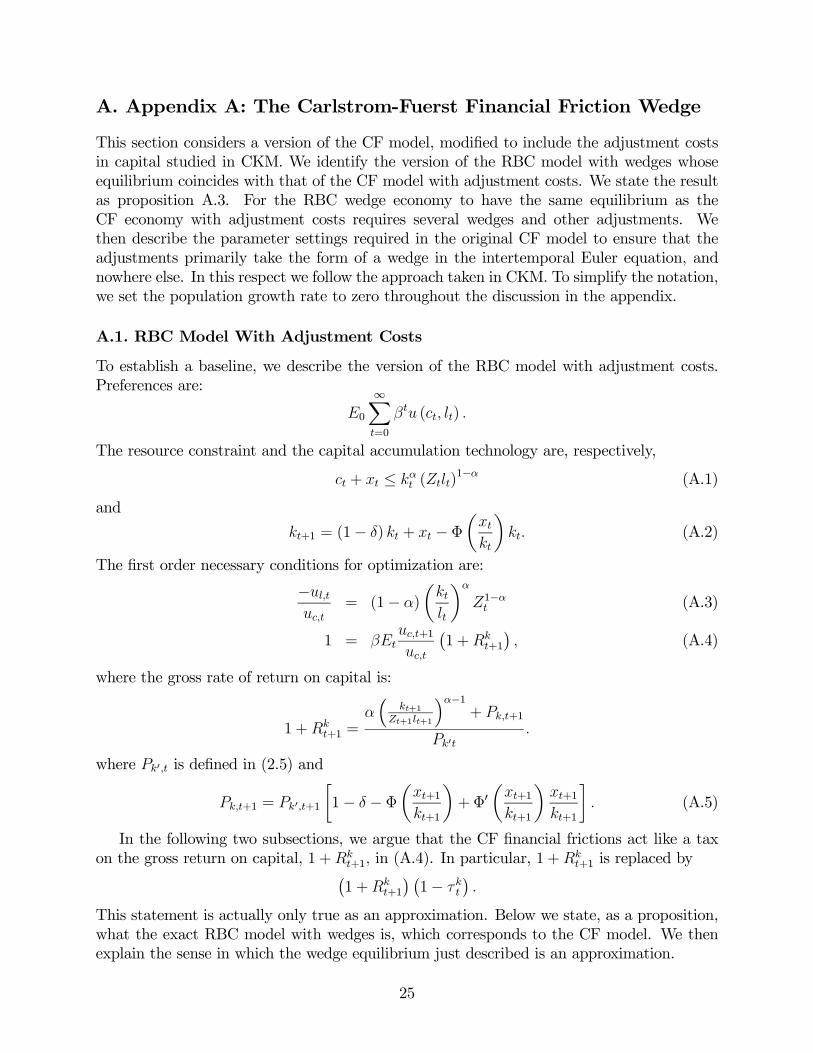
A. Appendix A: The Carlstrom-Fuerst Financial Friction Wedge

This section considers a version of the CF model, modified to include the adjustment costsin capital studied in CKM. We identify the version of the RBC model with wedges whoseequilibrium coincides with that of the CF model with adjustment costs. We state the resultas proposition A.3. For the RBC wedge economy to have the same equilibrium as theCF economy with adjustment costs requires several wedges and other adjustments. Wethen describe the parameter settings required in the original CF model to ensure that theadjustments primarily take the form of a wedge in the intertemporal Euler equation, andnowhere else. In this respect we follow the approach taken in CKM. To simplify the notation,we set the population growth rate to zero throughout the discussion in the appendix.

A.1. RBC Model With Adjustment Costs

To establish a baseline, we describe the version of the RBC model with adjustment costs.Preferences are:

E0

∞Xt=0

βtu (ct, lt) .

The resource constraint and the capital accumulation technology are, respectively,

ct + xt ≤ kαt (Ztlt)1−α (A.1)

and

kt+1 = (1− δ) kt + xt − Φ

µxtkt

¶kt. (A.2)

The first order necessary conditions for optimization are:

−ul,tuc,t

= (1− α)

µktlt

¶α

Z1−αt (A.3)

1 = βEtuc,t+1uc,t

¡1 +Rk

t+1

¢, (A.4)

where the gross rate of return on capital is:

1 +Rkt+1 =

α³

kt+1Zt+1lt+1

´α−1+ Pk,t+1

Pk0t.

where Pk0,t is defined in (2.5) and

Pk,t+1 = Pk0,t+1

∙1− δ − Φ

µxt+1kt+1

¶+ Φ0

µxt+1kt+1

¶xt+1kt+1

¸. (A.5)

In the following two subsections, we argue that the CF financial frictions act like a taxon the gross return on capital, 1 +Rk

t+1, in (A.4). In particular, 1 +Rkt+1 is replaced by¡

1 +Rkt+1

¢ ¡1− τkt

¢.

This statement is actually only true as an approximation. Below we state, as a proposition,what the exact RBC model with wedges is, which corresponds to the CF model. We thenexplain the sense in which the wedge equilibrium just described is an approximation.

25

A.2. The CF Model With Adjustment Costs

Here, we develop the version of the CF model in which there are adjustment costs in theproduction of new capital. The economy is composed of firms, an η mass of entrepreneurs anda mass, 1−η, of households. The sequence of events through the period proceeds as follows.First, the period t shocks are observed. Then, households and entrepreneurs supply labor andcapital to competitive factor markets. Because firm production functions are homogeneous,all output is distributed in the form of factor income. Households and entrepreneurs then selltheir used capital on a capital market. The total net worth of households and entrepreneurs atthis point consists of their earnings of factor incomes, plus the proceeds of the sale of capital.Households divide this net worth into a part allocated to current consumption, and a partthat is deposited in the bank. Entrepreneurs apply their entire net worth to a technologyfor producing new capital. They produce an amount of capital that requires more resourcesthan they can afford with only their own net worth. They borrow the rest from banks.At this point the entrepreneur experiences an idiosyncratic shock which is observed to him,while the bank can only see it by paying a monitoring cost. This creates a conflict betweenthe entrepreneur and the bank which is mitigated by the bank extending the entrepreneur astandard debt contract. After capital production occurs, entrepreneurs sell the new capital,and pay off their bank loan. Households receive a return on their deposits at the bank, anduse the proceeds to purchase new capital. Entrepreneurs use their income after paying offthe banks to buy consumption goods and new capital. All the newly produced capital ispurchased by households and entrepreneurs, and all the economy’s consumption goods areconsumed. The next period, everything starts all over.We now provide a formal description of the economy. The household problem is

max{cc,t,kct+1}∞t=0

∞Xt=0

βtu (ct, lt) ,

subject to:ct + qtkc,t+1 ≤ wc

t lt + [rt + Pk,t] kc,t (A.6)

where ct and kc,t denote household consumption and the household stock of capital, re-spectively. In addition, and lt denotes household employment, wc

t denotes the household’scompetitive wage rate, Pk,t denotes the price of used capital and qt denotes the price of capi-tal available for production in the next period (the reason for not denoting this price by Pk0,t

will be clear momentarily). After receiving their period t income, households allocate theirnet worth (the right side of (A.6)) to ct and the rest, wc

t lt+[rt + Pk,t] kc,t− ct, is deposited ina bank. These deposits earn a rate of return of zero. This is because markets are competitiveand the opportunity cost to the household of the output they lend to the bank is zero. Laterin the period, when the deposit matures, the households use the principal to purchase kc,t+1units of capital. The first order conditions of the household are (A.6) with the equality strictand:

1 = Etβuc,t+1uc,t

∙rt+1 + Pk,t+1

qt

¸(A.7)

−ul,tuc,t

= wet , (A.8)

26

where uc,t and −ul,t denote the time t marginal utilities of consumption and leisure, respec-tively.The η entrepreneurs’ present discounted value of utility is:

E0

∞Xt=0

(βγ)t cet.

After the period t shocks are realized, the net worth of entrepreneurs, at, is:

at = wet + [rt + Pk,t] ket,

where wet is the wage rate earned by the entrepreneur, who inelastically supplies his one

unit of labor. The entrepreneur uses the at consumption goods, together with a loan fromthe bank to purchase the inputs into the production of capital goods. Entrepreneurs haveaccess to the technology for producing capital, (2.1). The technology proceeds in two stages.In the first stage, the entrepreneur produces an intermediate input, it. In the second stage,that input results in ωit units of capital, which has a price, in consumption goods, qt. Therandom variable, ω, is independently distributed across entrepreneurs, has mean unity, andcumulative density function,

Ψ (z) ≡ prob [ω ≤ z] .

The entrepreneur who wishes to produce it units of the capital input faces the followingcost function:

C (it;Pk,t) = minϕk,t,ϕx,t

Pk,tϕk,t + ϕx,t + λt

∙it − (1− δ)ϕk,t − ϕx,t + Φ

µϕx,t

ϕk,t

¶ϕk,t

¸,

where the constraint is that the object in square brackets is no less than zero. In addition,ϕk,t and ϕx,t denote the quantity of old capital and investment goods, respectively, purchasedby the entrepreneur. The first order conditions for ϕk,t and ϕx,t are:

Pk,t = λt

∙1− δ − Φ

µϕx,t

ϕk,t

¶+ Φ0

µϕx,t

ϕk,t

¶ϕx,t

ϕk,t

¸(A.9)

1 = λt

∙1− Φ0

µϕx,t

ϕk,t

¶¸, (A.10)

respectively. The reason for denoting the time t price of old capital by Pk,t is now apparent.Substituting out for λ in (A.9) from (A.10), we see that the formula for Pk,t here coincideswith with the one implied by (A.5). The reason for not denoting the price of new capital byPk0,t is also apparent. Comparing (A.10) with (2.5) we see that the formula for λt coincideswith the formula for Pk0,t in the standard RBC model with adjustment costs. However, theequilibrium value of qt will not coincide with λt here. This is because λt does not capture allthe costs of producing new capital. It measures the marginal costs implied by the productiontechnology. However, as discussed in detail in CF, it is missing the marginal cost that arisesfrom the conflict between entrepreneurs and banks. This has the consequence that theproduction of capital necessarily involves some monitoring, and therefore also involves somedestruction of capital.

27

Solving (A.10) for xt/kt in terms of λt, and using the result to substitute out for ϕx,t/ϕk,t

in (A.9):

Pk,t = λt

⎡⎣(1− δ)− a

2

Ã1λt− 1a

!2+ a

Ã1λt− 1a

!Ã1λt− 1a

+ b

!⎤⎦Solving this for λt, provides the marginal cost function for producing it :

λt = λ (Pk,t) . (A.11)

Because all entrepreneurs face the same Pk,t, they will all choose the same ratio, ϕx,t/ϕk,t,regardless of the scale of production, it. Moreover, that ratio must be equal to the ratio ofaggregate investment to the aggregate stock of capital.The constant returns to scale feature of the production function implies that the total

cost of producing it is:

C (it;Pk,t) =

½λ (Pk,t) it a > 0

it a = 0

Consider an entrepreneur who has at units of goods and wishes to produce it ≥ at, so that theentrepreneur must borrow λ (Pk,t) it− at from the bank. Following CF, we suppose that theentrepreneur receives a standard debt contract. This specifies a loan amount and an interestrate, Ra

t , in consumption units. If the revenues of the entrepreneur turn out to be too low forhim to repay the loan, then the entrepreneur is ‘bankrupt’ and he simply provides everythinghe has to the bank. In this case, the bank pays a monitoring cost which is proportional tothe scale of the entprepeneur’s project, µiat . We now work out the equilibrium value of theparameters of the standard debt contract.The value of ω such that entrepreneurs with smaller values of ω are bankrupt, is ωa

t ,where

[λ (Pk,t) it − at]Rat = ωa

t itqt.

Using this we find that the average, across all entrepreneurs with asset level at, of revenuesis:

itqt

Z ∞

0

ωdF (ω)−Z ∞

ωat

Rat (λ (Pk,t) i

at − at) dF (ω)− itqt

Z ωat

0

ωdF (ω)

= itqtf (ωat ) ,

where

f (ωat ) =

Z ∞

ωat

ωdΦ (ω)− ωat (1− Φ (ωa

t )) .

The average receipts to banks, net of monitoring costs, across loans to all entprepreneurswith assets at is:

qtiat

∙Z ωat

0

ωdΦ (ω)− µΦ (ωat )

¸+ [λ (Pk,t) it − at]R

at [1− Φ (ωa

t )]

= qtiat g (ω

at ) ,

28

where

g (ωat ) =

Z ωat

0

ωdΦ (ω)− µΦ (ωat ) + ωa

t [1− Φ (ωat )] .

The contract with entrepreneurs with asset levels, at, that is assumed to occur in equi-librium is the one that maximizes the expected state of the entrepreneur at the end of thecontract, subject to the requirement that the bank be able to pay the household a grossrate of interest of unity. The interval during which the entrepreneur produces capital is onein which there is no alternative use for the output good. So, the condition that must besatisfied for the bank to participate in the loan contract is:

qtitg (ωat ) ≥ λ (Pk,t) it − at.

The contract solves the following Lagrangian problem:

maxωat ,it

itqtf (ωat ) + µ [qtitg (ω

at )− λ (Pk,t) it + at] .

The first order conditions for ωat and it are, after solving out for µ and rearranging:

qtf (ωat ) =

f 0 (ωat )

g0 (ωat )[qtg (ω

at )− λ (Pk,t)] (A.12)

it =at

λ (Pk,t)− qtg (ωat )

(A.13)

From (A.12), we see that ωat = ωt for all at, so that Ra

t = Rt for all at. It then follows from(A.13) that the loan amount is proportional to at. As in the no adjustment cost case in CF,these two properties imply that in studying aggregates, we can ignore the distribution ofassets across entrepreneurs.The expected net revenues of the entrepreneurs, expressed in terms of at, are, after making

use of (A.13):

itqtf (ωt) =qtf (ωt)

λ (Pk,t)− qtg (ωt)at. (A.14)

At the end of the period, after the debt contract with the bank is paid off, the entrepreneurswho do not go bankrupt in the process of producing capital have income that can be usedto buy consumption goods and new capital goods:

cet + qtket+1 ≤½

itqtω −Rt (λ (Pk,t) it − at) ω ≥ ωt

0 ω < ωt. (A.15)

An entrepreneur who is bankrupted in period t must set cet = 0 and ket+1 = 0. In periodt + 1, these entrepreneurs start with net worth at+1 = we

t+1. Entrepreneurs who are notbankrupted in period t can purchase positive amounts of cet and ke,t+1 (except in the non-generic case, ω = ωt). For these entrepreneurs, the marginal cost of purchasing ke,t+1 is qtunits of consumption. The time t expected marginal payoff from ke,t+1 at the beginning ofperiod t + 1 is Et [rt+1 + Pk,t+1] . In each aggregate state in period t + 1, the entrepreneurexpands his net worth by the value of [rt+1 + Pk,t+1] in that state. This extra net worthcan be leveraged into additional bank loans, which in turn permit an expansion in the

29

entrepreneur’s payoff by investing in the capital production technology. The expected valueof this additional payoff (relative to date t+1 idiosyncratic uncertainty) corresponds to thecoefficient on at in (A.14). So, the expected rate of return available to entrepreneurs whoare not bankrupt in period t is:

Et

∙rt+1 + Pk,t+1

qt× ζt+1

¸, (A.16)

which they equate to 1/(βγ). Here,

ζt+1 = max

∙qt+1f (ωt+1)

λ (Pk,t+1)− qt+1g (ωt+1), 1

¸.

The expression to the left of ‘×’ in (A.16) is the rate of return enjoyed by ordinary households.The reason that ζt+1 cannot be less than unity is that and entprepeneur can always obtainunity, simply by consuming his net worth in the following period and not producing anycapital. Averaging over all budget constraints in (A.15):

cet + qtket+1 =qtf (ωt)

λ (Pk,t)− qtg (ωt)at.

Here, cet and ke,t+1 refer to averages across all entrepreneurs.Output is produced by goods-producers using a linear homogeneous technology,

y (kt, lt, η, Zt) = kαt ((1− η)Ztlt)1−α−ζ ηζ , (A.17)

where kt is the sum of the capital owned by households and the average capital held byentrepreneurs:

kt = (1− η) kct + ηke,t.

The argument, η, in y is understood to apply to the second occurrence of η. The argumentsin the production function reflect our assumption that the entrepreneur supplies one unit oflabor, and households supply lt units of labor. Profit maximization implies:

yk,t = rt, yl,t = wct , y3,t = we

t . (A.18)

We now collect the equilibrium conditions for the economy. The production of new capitalgoods by the average entrepreneur is:

it

Z ∞

0

ωdF (ω)− µit

Z ωt

0

dF (ω)

= it [1− µF (ωt)] .

Since there are η entprepreneurs, the total new capital produced is kt+1 = ηit [1− µF (ωt)] ,so that

kt+1 =

∙(1− δ) kt + xt − Φ

µxtkt

¶kt

¸[1− µF (ωt)] . (A.19)

The resource constraint is:

(1− η) ct + ηcet + xt = kαt ((1− η)Ztlt)1−α−ζ ηζ . (A.20)

30

Substituting (A.18) into (A.7) and (A.8):

1 = βEtuc,t+1uc,t

yk,t+1 + Pk,t+1

qt(A.21)

−ul,tuc,t

= yl,t. (A.22)

The budget constraint of the entrepreneur is:

cet + qtket+1 = λ (Pk,t)kt+1

η [1− µF (ωt)]qtf (ωt) (A.23)

The efficiency conditions associated with the contract are:

qtf (ωt) =f 0 (ωt)

g0 (ωt)[qtg (ωt)− λ (Pk,t)] (A.24)

kt+1η [1− µF (ωt)]

=at

λ (Pk,t)− qtg (ωt)(A.25)

at = y3,t + yk,tket + Pk,tket (A.26)

The intertemporal efficiency condition for the entrepreneur is (assuming the condition, ζt+1 ≥1, is not binding):

Et

∙Fk,t+1 + Pk,t+1

qt× qt+1f (ωt+1)

λ (Pk,t+1)− qt+1g (ωt+1)

¸=1

γβ(A.27)

Taking the ratio of (A.9) to (A.10), we obtain:

Pk,t =1− δ − Φ

³xtkt

´+ Φ0

³xtkt

´xtkt

1− Φ0³xtkt

´ (A.28)

The 10 variables to be determined with the 10 equations, (A.19)-(A.28) are: ct, ce,t, xt, kt,ke,t, lt, Pk,t, qt, ωt, at.It is convenient to define a sequence of markets equilibrium formally. Let st denote a

history of realizations of shocks. Then,

Definition A.1. An equilibrium of the CF economy with adjustment costs is a sequence ofprices, {Pk (s

t) , q (st) , we (st) , wc (st) , r (st)} , quantities, {c (st) , ce (st) , x (st) , k (st) , ke (st) , l (st) , a (st)} ,and {ω (st)} such that:(i) Households optimize (see (A.21), (A.22))(ii) Entrepreneurs optimize (see (A.23), (A.26), (A.27), (A.28))(iii) Firms optimize (see (A.18))(iv) Conditions related to the standard debt contract are satisfied (see (A.24), (A.25))(v) The resource constraint and capital accumulations equations are satisfied (see (A.19),

(A.20))

31

A.3. The CF Model as an RBC Model with Wedges

We now construct a set of wedges for the RBC economy in section A.1, such that theequilibrium for the distorted version of that economy coincides with the equilibrium for theCF economy. We begin by constructing the following state-contingent sequences:

ψ¡st¢= 1− µF

¡eω ¡st¢¢ , (A.29)

τx¡st¢=

ψ (st) q (st)

λ³Pk,t (st)

´ − 1,θ¡st¢=

Pk (st) τx (s

t)

r (st),

G¡st¢= η

¡ce¡st¢− c

¡st¢¢

,

T¡st¢= G

¡st¢− τx

¡st¢x¡st¢− θ

¡st¢r¡st¢k¡st−1

¢,

D¡st¢= we

¡st¢η,

where q, ce, c, we, r, k, x, eω and Pk correspond to the objects without ‘ · ’ in a CF equilibrium.Also, λ is the function defined in (A.11). In this subsection, we treat D, ψ, θ, τx, G and Tas given exogenous stochastic processes, outside the control of agents. Here, D, G, and Trepresent exogenous sequences of profits, government spending and lump sum taxes. Also,θ and τx are tax rates on capital rental income and investment good purchases. Finally, ψis a technology shock in the production of physical capital.Consider the following budget constraint for the household:

c¡st¢+¡1 + τx

¡st¢¢

x¡st¢

(A.30)

≤¡1− θ

¡st¢¢

r¡st¢k¡st−1

¢+ w

¡st¢l¡st¢− T

¡st¢+D

¡st¢.

Here, r is the rental rate on capital, w is the wage rate, and l measures the work effort of thehousehold. Each of these variables is a function of st and is determined in an RBC wedgeeconomy. At time 0 the household takes prices, taxes and k (s−1) as given and chooses c, kand l to maximize utility:

∞Xt=0

Xst

βtπ¡st¢u¡c¡st¢, l¡st¢¢

subject to the budget constraint, no-Ponzi game and non-negativity constraints. Here, π (st)is the probability of history, st.Households operate the following backyard technology to produce new capital:

k¡st¢=

∙(1− δ) k

¡st¢+ x

¡st¢− Φ

µx (st)

k (st−1)

¶k¡st−1

¢¸ψ¡st¢. (A.31)

32

The first order necessary conditions for household optimization are:

ul¡st¢+ uc

¡st¢w¡st¢= 0, (A.32)

1 + τx (st)

ψ (st)Pk0¡st¢

(A.33)

=Xst+1|st

βπ¡st+1|st

¢ uc (st+1)uc (st)

£r¡st+1

¢ ¡1− θ

¡st+1

¢¢+¡1 + τx

¡st+1

¢¢Pk

¡st+1

¢¤,

where

Pk

¡st¢≡1− δ − Φ

µx(st)k(st)

¶+ Φ0

µx(st)k(st)

¶x(st)k(st)

1− Φ0³

x(st)k(st−1)

´ . (A.34)

Equation (A.32) is the first order condition associated with the optimal choice of l (st) .Equation (A.33) combines the first order order conditions associated with the optimal choiceof x (st) and k (st) . Also,

Pk0¡st¢≡ 1

1− Φ0³

x(st)k(st−1)

´ , (A.35)

is the pre-tax marginal cost of producing new capital, in units of the consumption good. Inaddition, π (st+1|st) ≡ π (st+1) /π (st) is the conditional probability of history st+1 given st.The technology for firms is taken from (A.17):

y (k, l, η, Z) = kα ((1− η)Zl)1−α−ζ ηζ ,

where, as before, the third argument in y refers only to the second occurrence of η. There arethree inputs: physical capital, household labor and another factor whose aggregate supplyis fixed at η. Profit maximization leads to:

r¡st¢= yk

¡st¢, w

¡st¢= yl

¡st¢, we

¡st¢= yη

¡st¢. (A.36)

The household is assumed to own the representative firm, and it receives the earnings ofη in the form of lump-sum profits, D (st) . We do allow allow trade in claims on firms, arestriction that is non-binding on allocations because the households are identical.We now state the equilibrium for the RBC wedge economy:

Definition A.2. AnRBCwedge equilibrium is a set of quantities, {c (st) , l (st) , k (st) , x (st)} ,and prices {Pk (s

t) , Pk0 (st) , r (st) , w (st)} , and a set of taxes, profits and government spend-

ing, {G (st) , τx (st) , θ (st) , T (st)} , technology shocks, {Z (st) , ψ (st)} , such that(i) The quantities solve the household problem given the prices, taxes, profits, government

spending and the shock to the backyard investment technology(ii) Firm optimization is satisfied(iii) Relations (A.29) is satisfied, for given state-contingent sequences, q, ce, c, we, r, k,

x, eω and Pk.

33

The variables to be determined in an RBC wedge equilibrium are c, l, k, x, Pk, Pk0 , r andw. The 8 equations that can be used to determine these are (A.30)-(A.36). It is easily verifiedthat c, l, k, x, Pk, r and w coincide with the corresponding objects in a CF equilibrium. Inaddition, Pk0 coincides with λ (Pk) in a CF equilibrium. To see this, one verifies that theequilibrium conditions in the RBC wedge economy coincide with the equilibrium conditionsin the CF economy. First, (A.31) coincides with (A.19). After using (A.36), we see that(A.32) coincides with (A.22). Consider the household budget equation evaluated at equality.Substituting out for lump sum transfers:

c¡st¢+¡1 + τx

¡st¢¢

x¡st¢

=¡1− θ

¡st¢¢

r¡st¢k¡st−1

¢+ w

¡st¢l¡st¢

τx¡st¢x¡st¢+ θ

¡st¢r¡st¢k¡st−1

¢+ we

¡st¢η +G

¡st¢,

or,

(1− η) c¡st¢+ x

¡st¢+ ηce

¡st¢

(A.37)

= r¡st¢k¡st−1

¢+ w

¡st¢l¡st¢+ we

¡st¢η

= y¡k¡st−1

¢, l¡st¢, η, Z

¡st¢¢

,

by linear homogeneity. Here, Z (st) = Z (st) , where st is the realization of period t uncertainty.Equation (A.37) coincides with (A.20). Substitute out for θ and τx from (A.29) into (A.33),and rearranging, we obtain:

1 = Etuc (s

t+1)

uc (st)

"r (st+1) + Pk (s

t+1)1+τx(st)ψ(st)

Pk0 (st)

#.

Note that by definition of 1 + τx (st) in (A.29),

1 + τx (st)

ψ (st)Pk0¡st¢=

Pk0 (st) q (st)

λ (Pk,t (st)).

Combining (A.11) and (A.10), we find that λ (Pk,t (st)) = Pk0 (s

t) , so that the household’sintertemporal Euler equation reduces to (A.21), or (after making use of (A.36)):

Etuc (s

t+1)

uc (st)

∙yk (s

t+1) + Pk (st+1)

Pk0 (st)

¡1− τk

¡st¢¢¸

= 1, (A.38)

where

1− τk¡st¢=

ψ (st)

1 + τx (st).

We conclude that conditions (A.19)-(A.22) in the CF economy are satisfied. The remainingequilibrium conditions are satisfied, given (A.29). We state this result as a proposition:

Proposition A.3. Consider a CF equilibrium, and a set of taxes, technology shocks andtransfers computed in (A.29). The objects, {c (st) , l (st) , k (st) , x (st)} , {Pk (s

t) , r (st) , w (st)}and Pk0 (s

t) = λ (Pk (st)) in the CF equilibrium correspond to an RBC wedge equilibrium.

For η and ζ close to zero and ψ close to unity, the RBC wedge equilibrium converges tothe equilibrium conditions of the RBC model with adjustment costs in section A.1 with awedge, 1− τk, in the intertemporal Euler equation, (A.4).

34

B. Appendix B: The Bernanke-Gertler-Gilchrist Financial FrictionWedge

In this section we briefly review the BGG model and derive the RBC wedge model to whichit corresponds. In the model there are households, capital producers, entrepreneurs andbanks. At the beginning of the period, households supply labor to factor markets, andentrepreneurs supply capital. Output is then produced and an equal amount of incomeis distributed among households and entrepreneurs. Households then make a deposit withbanks, who lend the funds on to entrepreneurs. Entrepreneurs have a special expertise inthe ownership and management of capital. They have their own net worth with which toacquire capital. However, it is profitable for them to leverage this net worth into loans frombanks, and acquire more capital than they can afford with their own resources. The source offriction is a particular conflict between the entrepreneur and the bank. In the managementof capital, idiosyncratic things happen, which either make the management process moreprofitable than expected, or less so. The problem is that the things that happen in thisprocess are observed only by the entrepreneur. The bank can observe what happens insidethe management of capital, but only at a cost. As a result, the entrepreneur has an incentiveto underreport the results to the bank, and thereby attempt to keep a greater share of theproceeds for himself. To mitigate this conflict, it is assumed that entrepreneurs receive astandard debt contract from the bank.The capital that entrepreneurs purchase at the end of the period is sold to them by

capital producers. The latter use the old capital used within the period, as well as investmentgoods, to produce the new capital that is sold to the entrepreneurs. Capital producers haveno external financing need. They finance the purchase of used capital and investment goodsusing the revenues earned from the sale of new capital.The budget constraint of households is:

ct +Bt+1 ≤ (1 +Rt)Bt + wtlt + Tt,

where Rt denotes the interest earned on deposits with the bank, bt denotes the beginning-of-period t stock of those deposits, wt denotes the wage rate, lt denotes employment and Ttdenotes lump sum transfers. Subject to this budget constraint and a no-Ponzi condition,households seek to maximize utility:

E0

∞Xt=0

βtu (ct, lt) .

Households’ first order conditions, in addition to the transversality condition, are:

uc,t = βEtuc,t (1 +Rt+1)−ul,tuc,t

= wt.

Firms have the following production function:

yt = kαt (Ztlt)1−α = y (kt, lt, Zt) .

35

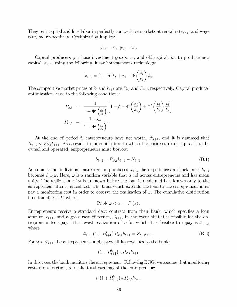
They rent capital and hire labor in perfectly competitive markets at rental rate, rt, and wagerate, wt, respectively. Optimization implies:

yk,t = rt, yl,t = wt.

Capital producers purchase investment goods, xt, and old capital, kt, to produce newcapital, kt+1, using the following linear homogeneous technology:

kt+1 = (1− δ) kt + xt − Φ

µxtkt

¶kt.

The competitive market prices of kt and kt+1 are Pk,t and Pk0,t, respectively. Capital produceroptimization leads to the following conditions:

Pk,t =1

1− Φ0³xtkt

´ ∙1− δ − Φ

µxtkt

¶+ Φ0

µxtkt

¶xtkt

¸

Pk0,t =1 + gn

1− Φ0³xtkt

´ .At the end of period t, entrepreneurs have net worth, Nt+1, and it is assumed that

Nt+1 < Pk0,tkt+1. As a result, in an equilibrium in which the entire stock of capital is to beowned and operated, entprepreneurs must borrow:

bt+1 = Pk0,tkt+1 −Nt+1. (B.1)

As soon as an individual entrepreneur purchases kt+1, he experiences a shock, and kt+1becomes kt+1ω. Here, ω is a random variable that is iid across entrepreneurs and has meanunity. The realization of ω is unknown before the loan is made and it is known only to theentrepreneur after it is realized. The bank which extends the loan to the entrepreneur mustpay a monitoring cost in order to observe the realization of ω. The cumulative distributionfunction of ω is F, where

Pr ob [ω < x] = F (x) .

Entrepreneurs receive a standard debt contract from their bank, which specifies a loanamount, bt+1, and a gross rate of return, Zt+1, in the event that it is feasible for the en-trepreneur to repay. The lowest realization of ω for which it is feasible to repay is ωt+1,where

ωt+1

¡1 +Rk

t+1

¢Pk0,tkt+1 = Zt+1bt+1. (B.2)

For ω < ωt+1 the entrepreneur simply pays all its revenues to the bank:¡1 +Rk

t+1

¢ωPk0,tkt+1.

In this case, the bank monitors the entrepreneur. Following BGG, we assume that monitoringcosts are a fraction, µ, of the total earnings of the entrepreneur:

µ¡1 +Rk

t+1

¢ωPk0,tkt+1.

36

At time t the bank borrows bt+1 from households. In each state of t + 1 the bank payshouseholds

(1 +Rt+1) bt+1 (B.3)

units of currency. The bank’s source of funds in each state of period t+1 is the earnings fromnon-bankrupt entrepreneurs plus the earnings of bankrupt entrepreneurs, net of monitoringcosts:

[1− F (ωt+1)]Zt+1bt+1 + (1− µ)

Z ωt+1

0

ωdF (ω)¡1 +Rk

t+1

¢Pk0,tkt+1. (B.4)

We follow BGG, who implicitly suppose that at date t there are no state-contingent marketsfor currency in date t+ 1. As a consequence, (B.3) must not exceed (B.4) in any date t+ 1state. This condition, together with competition among banks, leads to:

[1− F (ωt+1)]Zt+1bt+1 + (1− µ)

Z ωt+1

0

ωdF (ω)¡1 +Rk

t+1

¢Pk0,tkt+1 = (1 +Rt+1) bt+1.

Substituting from (B.2) for Zt+1bt+1 and dividing by¡1 +Rk

t+1

¢Pk0,tkt+1 :

[1− F (ωt+1)] ωt+1 + (1− µ)

Z ωt+1

0

ωdF (ω) =

µ1 +Rt+1

1 +Rkt+1

¶bt+1

Pk0,tkt+1.

We conclude that the gross return on capital can be expressed:

1 +Rt+1 =¡1− τkt+1

¢ ¡1 +Rk

t+1

¢,

where the ‘wedge’, 1− τkt+1, satisfies:

1− τkt+1 =Pk0,tkt+1

Pk0,tkt+1 −Nt+1

µ[1− F (ωt+1)] ωt+1 + (1− µ)

Z ωt+1

0

ωdF (ω)

¶.

The wedge, τkt , contains two additional endogenous variables, Nt+1 and ωt+1. These aredetermined in general equilibrium by the introduction of two additional equations: the con-dition associated with the fact that the standard debt contract maximizes the utility of theentrepreneur, as well as the law of motion for entrepreneurial net worth.The resource constraint for this economy is:

ct +Gt + xt = kαt (Ztlt)1−α ,

where Gt includes any consumption of entrepreneurs, as well as monitoring costs incurredby banks. As long as these latter can be ignored, then the BGG financial friction is to, ineffect, introduce a tax on the rate of return on capital in, 1 +Rk

t+1, in (A.4). In particular,1 +Rk

t+1 is replaced by ¡1 +Rk

t+1

¢ ¡1− τkt+1

¢.

Note there is a slight difference with CF financial frictions in that the latter imply the taxrate is not a function of period t + 1 uncertainty, while the BGG frictions imply that ingeneral it is a function of this uncertainty.

37

C. Appendix C: Other Empirical Results

Figures A1 - A9 display additional results for US recessions. Figures A1-A8 pertain to fourpostwar US recessions. Figures A1 - A4 are the analog of Figure 3 for the 1982 recession.Figures A5 - A8 are the analog of Figure 4. Figure A9 is the analog of Figure 6 for the USGreat Depression, except that it is based on BCA, when measurement error is set to zero inestimation.

38

References

[1] Abel, Andrew, 1980, “Empirical investment equations: An integrative framework,”Carnegie-Rochester Conference Series on Public Policy, vol. 12, pp. 39—91.

[2] Bernanke, Ben, Mark Gertler, and Simon Gilchrist, 1999, “The Financial Acceleratorin a Quantitative Business Cycle Framework,” Handbook of Macroeconomics, editedby John B. Taylor and Michael Woodford, pp. 1341-1393, Amsterdam, New York andOxford, Elsevier Science, North-Holland.

[3] Boldrin, Michele, Lawrence J. Christiano and Jonas Fisher, 2001, ‘Habit Persistence,Asset Returns and the Business Cycle’, American Economic Review, vol. 91, no. 1, pp.149-166. March.

[4] Carlstrom, Charles, and Timothy Fuerst, 1997, “Agency Costs, Net Worth, and Busi-ness Fluctuations: A Computable General Equilibrium Analysis,” American EconomicReview, 87, 893-910.

[5] Chari, V.V., Patrick Kehoe and Ellen McGrattan, 2006, “Business Cycle Accounting,”Federal Reserve Bank of Minneapolis Staff Report 328, revised February.

[6] Christiano, Lawrence J., 2002, ‘Solving Dynamic Equilibrium Models by a Method ofUndetermined Coefficients,’ Computational Economics, October, Volume 20, Issue 1-2.

[7] Christiano, Lawrence J., Martin Eichenbaum and Charles Evans, 2005, ‘Nominal Rigidi-ties and the Dynamic Effects of a Shock to Monetary Policy’, Journal of Political Econ-omy.

[8] Christiano, Lawrence J., Martin Eichenbaum and Robert Vigfusson, 2006, ‘AssessingStructural VARs,’ forthcoming, Macroeconomics Annual, edited by George-Marios An-geletos, Kenneth Rogoff, and Michael Woodford.

[9] Christiano, Lawrence J., Roberto Motto and Massimo Rostagno, 2004, ‘The US GreatDepression and the Friedman-Schwartz Hypothesis,’ Journal of Money, Credit andBanking.

[10] Christiano, Lawrence J., Roberto Motto and Massimo Rostagno, 2006, ‘Financial Fac-tors in Business Cycles,’ manuscript.

[11] Cochrane, John H., and Lars Peter Hansen, 1992, ‘Asset pricing explorations for macro-economics,’ NBER Macroeconomics Annual, pp. 115—165.

[12] Eberly, Janice C., 1997, ‘International Evidence on Investment and Fundamentals,’European Economic Review, vol. 41, no. 6, June, pp. 1055-78.

[13] Erceg, Christopher J., Henderson, Dale, W. and Andrew T. Levin, 2000, ‘Optimal Mone-tary Policy with Staggered Wage and Price Contracts,’ Journal of Monetary Economics,46(2), October, pages 281-313.

39

[14] Fernandez-Villaverde, Jesus, Juan F. Rubio-Ramirez and Thomas J. Sargent, 2006, ‘A,B, C ’s (and D)’s For Understanding VARs,’ manuscript.

[15] Gali, Jordi, Mark Gertler and J. David Lopez-Salido, 2003, ‘Markups, Gaps, and theWelfare Costs of Business Fluctuations,’ forthcoming, Review of Economics and Statis-tics.

[16] Hall, Robert, 1997, ‘Macroeconomic Fluctuations and the Allocation of Time,’ Journalof Labor Economics, 15 (part 2) , S223-S250.

[17] Hamilton, James B. (1994). Time Series Analysis. Princeton: Princeton UniversityPress.

[18] Ingram, Beth, Narayana Kocherlakota and N. Savin, 1994, “Explaining Business Cycles:A Multiple-Shock Approach,” Journal of Monetary Economics, 34, 415-428.

[19] Lippi, Marco, and Lucrezia Reichlin, 1993, ‘The Dynamic Effects of Aggregate Demandand Supply Disturbances: Comment,’ The American Economic Review, Vol. 83, No. 3(June), pp. 644-652.

[20] Lucca, David, 2006, ‘Resuscitating Time to Build,’ manuscript, Board of Governors ofthe Federal Reserve.

[21] Matsuyama, Kiminori, 1984, ‘A Learning Effect Model of Investment: An AlternativeInterpretation of Tobin’s Q’, unpublished manuscript, Northwestern University.

[22] Mulligan, Casey, 2002, ‘A Dual Method of Empirically Evaluating Dynamic CompetitiveModels with Market Distortions, Applied to the Great Depression and World War II,’National Bureau of Economic Research Working Paper 8775.

[23] Parkin, Michael, 1988, ‘A Method for Determining Whether Parameters in AggregativeModels are Structural,’ Carnegie-Rochester Conference Series on Public Policy, 29, 215-252.

[24] Queijo, Virginia, 2005, “How Important are Financial Frictions in the US and the EuroArea?”, Seminar paper no. 738, Institute for International Economic Studies, StockholmUniversity, August.

[25] Rosen, Sherwin and Robert Topel, 1988, ‘Housing Investment in the United States,’Journal of Political Economy, Vol. 96, No. 4 (Aug.), pp. 718-740

[26] Sargent, Thomas, 1989, ‘Two Models of Measurements and the Investment Accelerator,’Journal of Political Economy, vol. 97, issue 2, April, pp. 251-287.

[27] Schmitt-Grohe, Stephanie, and Martin Uribe, 2004, ‘Solving Dynamic General Equilib-rium Models Using a Second-Order Approximation to the Policy Function,’ Journal ofEconomic Dynamics and Control, 28.

[28] Sims, Christopher A. and Tao Zha, 1996, ‘Does Monetary Policy Generate Recessions?’,forthcoming as a ‘vintage paper’ in Macroeconomic Dynamics.

40

[29] Uhlig, Harald, 2002, ‘What Moves Real GNP?’, manuscript, Humboldt Unversity Berlin.

[30] Wan, E.A. and R. van der Merwe, 2001, "Kalman Filtering and Neural Networks",chap. Chapter 7 : The Unscented Kalman Filter, (50 pages), Wiley Publishing, Eds. S.Haykin.

41

Table 1: Summary of Results for the 1982 US RecessionPanel 1a: CKM Version of Intertemporal Wedge (τx,t)

CKM measurement error No measurement errorbaseline rotation baseline rotation

Tobin’s q elasticity = ∞

-0.03 0.92 0.047 0.96

Tobin’s q elasticity = 1

0.31 1.02 0.28 1.05

Panel 1b: Alternative Version of the Wedge (BGG, τkt )Likelihood ratio test of CKM measurement error No measurement errorCKM measurement error baseline rotation baseline rotation

Tobin’s q elasticity = ∞

481 0.24 1.32 -1.31 -0.01

Tobin’s q elasticity = 1

541 0.22 1.05 0.53 0.93

Notes: (1) Likelihood ratio statistic - twice difference between the log likelihoodunder estimation with CKM measurement error specification, and under estimationwith measurement error set to zero; (2) CKM measurement error: results basedon estimation with CKM specification of R in (3.6),(3) No measurement error: based on estimation subject to R = 0, (4) baselinedecomposition - see text, (5) rotation - rotation of shocks which maximizesimportance of financial frictions, as defined in text.

1

Table 2: Alternative Version of the Wedge (BGG, τkt )Panel A: Tobin’s q Elasticity = ∞

CKM Measurement Error No Measurement Error

Baseline Rotation Ratio Baseline Rotation RatioCountry

United States 0.24 0.90 0.49 -1.11 -0.15 1.29Belgium 0.61 0.83 0.28 -1.12 0.24 0.31Canada 0.20 1.11 0.69 -0.51 0.95 1.25Denmark 0.39 1.15 0.00 0.18 1.11 0.92Finland 1.18 1.58 0.13 0.24 1.31 0.44France 0.13 1.63 0.96 -3.10 1.59 0.41Germany 0.44 1.10 0.77 -1.87 -3.29 0.00Italy -4.83 1.85 0.00 -0.19 1.38 0.45Japan -0.00 1.02 1.01 0.27 1.67 1.41Mexico 0.00 1.06 1.00 -0.07 1.05 1.00Netherlands 2.50 3.02 0.04 -0.01 1.25 0.68Norway 1.27 -0.23 0.00 -0.56 0.79 0.90Spain 1.49 1.51 0.00 -0.00 1.66 0.97Switzerland -0.14 0.95 1.03 -0.24 0.89 1.01England 0.25 1.10 0.60 0.04 1.19 0.89Weighted Mean 0.22 1.30 0.44 -0.59 0.80 0.85

Panel B: Tobin’s q Elasticity = 1

CKM Measurement Error No Measurement Error

Baseline Rotation Ratio Baseline Rotation RatioCountry

United States 0.15 0.89 0.73 0.46 0.85 0.30Belgium -0.09 0.85 1.01 -0.69 1.25 1.39Canada 0.33 1.26 0.55 0.75 1.86 0.39Denmark 0.14 1.05 0.99 -0.17 0.95 1.12Finland -6.25 -5.72 0.02 -0.60 0.49 0.33France 1.45 1.43 0.02 1.13 0.99 0.02Germany 0.33 1.08 1.32 -0.08 0.90 1.22Italy 0.66 1.29 0.41 -0.51 3.72 0.11Japan 0.71 1.05 1.12 0.23 2.06 1.01Mexico -0.04 0.92 1.06 0.40 1.04 0.41Netherlands 0.76 1.25 0.43 0.04 1.51 0.65Norway -0.06 1.10 0.91 -0.29 1.53 0.78Spain 1.93 1.28 0.03 0.67 1.29 0.96Switzerland 0.31 1.11 0.67 -0.14 1.38 0.24England -0.01 1.07 0.91 -0.08 1.26 1.24Weighted Mean -0.01 0.61 0.61 0.16 1.37 0.60

1

1960 1970 1980 1990 2000

-5

0

5

10

1960 1970 1980 1990 2000

-6

-4

-2

0

2

4

6

8

10

12

1960 1970 1980 1990 2000

-6

-4

-2

0

2

4

6

8

10

12

Figure 1A: Actual and Model Rates of Return, Different Tobin's q Elasticities

1960 1970 1980 1990 2000

-6

-4

-2

0

2

4

6

8

10

12

Tobin's q elasticity = 1/2data

Tobin's q elasticity = 1data

Tobin's q elasticity = 3data

Tobin's q elasticity = infinitydata

40 60 80 100 120 140 1600

1

2

3

4

5

Investment-capital ratio, as a percent of steady state, 100 t

Adju

stm

ent costs

, as p

erc

ent of aggre

gate

outp

ut

Figure 1B: Implications of Quadratic and Alternative Adjustment Cost Functions, Each Having Unit Tobin's q Elasticity

Quadratic Adjustment CostsAlternative Adjustment Costs

Fundamental

Economic

Disturbances

Other disturbances

(tastes, government

spending, technology,

etc.)

Financial friction

disturbances

(monitoring costs,

entrepreneurial risk,

etc.)

Wedges,

or Shocks

Other wedges: shock in

intratemporal Euler

equation, shock in

resource constraint

Intertemporal wedge:

shock that enters

intertemporal Euler

equation

Propagation

(*)

(ii)

(iii)

(i)

(*) movements in other wedges due to other disturbances

(i) movements in the intertemporal wedge due to financial disturbances

(ii) movements in the intertemporal wedge due to spillover effects from standard

disturbances

(iii) movements in other wedges due to spillovers from financial disturbances

Figure 2: The propagation of economic disturbances through wedges

1980 1981 1982 1983 1984 1985

0.95

1

1.05

1.1

Outp

ut

Tobin's Q Elasticity =

1980 1981 1982 1983 1984 1985

1

1.5

2

Investm

ent

1980 1981 1982 1983 1984 1985

0.95

1

1.05

1.1

1.15

Hours

1980 1981 1982 1983 1984 1985

0.8

0.9

1

Consum

ption

1980 1981 1982 1983 1984 1985

0.92

0.94

0.96

0.98

1

Tobin's Q Elasticity = 1

1980 1981 1982 1983 1984 1985

0.8

0.9

1

1980 1981 1982 1983 1984 1985

0.94

0.96

0.98

1

1.02

Figure 3: Raw Data ('All Wedges') and Various Counterfactual Simulations

1980 1981 1982 1983 1984 1985

0.94

0.96

0.98

1

1.02

Intertemporal Wedge, ME = 0Intertemporal Wedge, ME = CKMAll WedgesBaseline

1980 1981 1982 1983 1984 1985

0.92

0.94

0.96

0.98

1Wedge=0.52742 R

2=0.86969 =2.0858

GD

P

1980 1981 1982 1983 1984 1985

0.8

0.9

1

Wedge=1.1727 R2=0.93033 =1.1072

INV

ES

TM

EN

T

1980 1981 1982 1983 1984 1985

0.94

0.96

0.98

1

1.02

Wedge=0.91634 R2=0.85922 =1.2317

HO

UR

S

1980 1981 1982 1983 1984 1985

0.94

0.96

0.98

1

1.02

Wedge=-0.32052 R2=0.44068 =-1.0051

CO

NS

UM

PT

ION

BASELINE DECOMPOSITION

1980 1981 1982 1983 1984 1985

0.92

0.94

0.96

0.98

1

1.02

Wedge=0.92998 R2=0.87408 =0.80766

1980 1981 1982 1983 1984 1985

0.8

0.9

1

Wedge=0.87435 R2=0.98008 =1.1342

1980 1981 1982 1983 1984 1985

0.95

1

1.05

Wedge=0.54225 R2=0.75622 =0.83027

Figure 4: Raw Data ('all wedges') and Two Counterfactual Wedges, Tobin's q = 1, No Measurement Error

1980 1981 1982 1983 1984 1985

0.94

0.96

0.98

1

Wedge=1.0783 R2=0.96272 =0.83927

ROTATION DECOMPOSITION

All WedgesIntertemporal WedgeBaseline

Note (1) wedge - fraction of fall in raw data at the trough for output accounted for by the intertemporal wedge; (2) R2 - R-square in regression of raw data on

wedge component throughout recession episode; (3) - slope coefficient in preceding regression

1900 1910 1920 1930 1940-70

-60

-50

-40

-30

-20

-10

0

10

20Figure 5D: Percent Euler Errors, Investment

perc

ent

year

1900 1910 1920 1930 1940-8

-6

-4

-2

0

2

4Figure 5A: Percent Euler Errors, Output

perc

ent

year

1900 1910 1920 1930 1940-6

-4

-2

0

2

4Figure 5B: Percent Euler Errors, Consumption

perc

ent

year

1900 1910 1920 1930 1940-12

-10

-8

-6

-4

-2

0

2

4

6Figure 5C: Percent Euler Errors, Hours

perc

ent

year

nonlinearlinear

nonlinearlinear

nonlinearlinear

nonlinearlinear

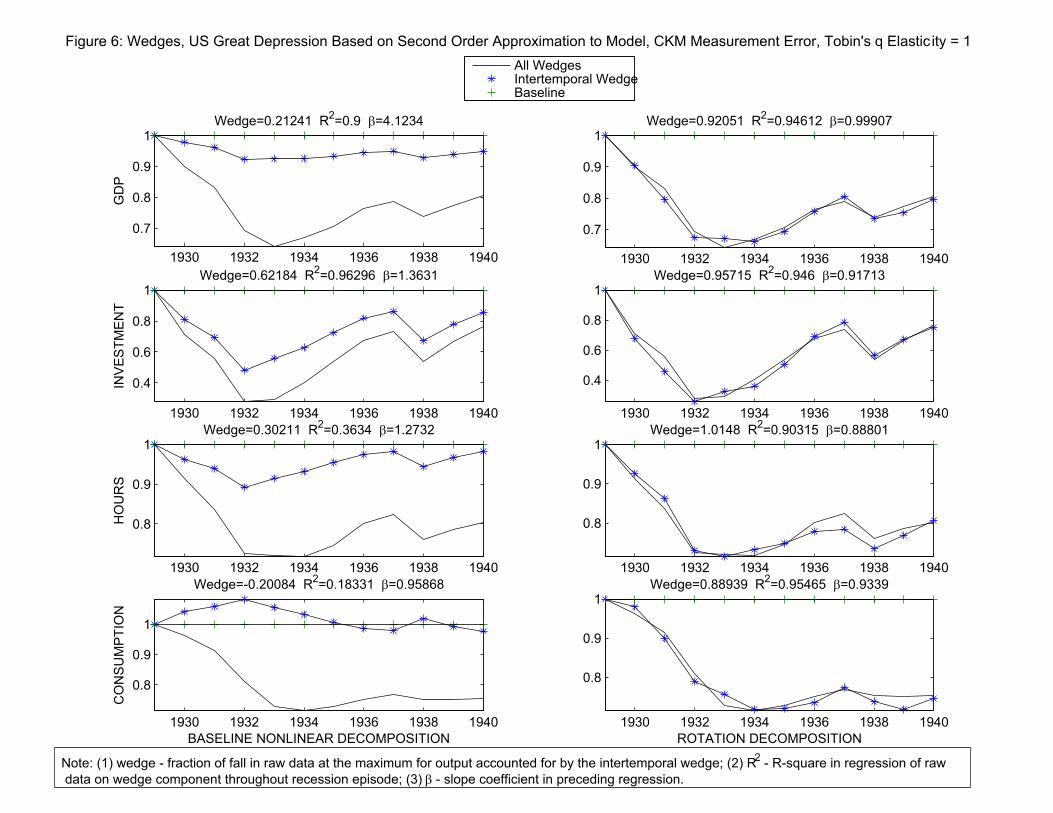
1930 1932 1934 1936 1938 1940

0.7

0.8

0.9

1Wedge=0.21241 R

2=0.9 =4.1234

GD

P

1930 1932 1934 1936 1938 1940

0.4

0.6

0.8

1Wedge=0.62184 R

2=0.96296 =1.3631

INV

ES

TM

EN

T

1930 1932 1934 1936 1938 1940

0.8

0.9

1Wedge=0.30211 R

2=0.3634 =1.2732

HO

UR

S

1930 1932 1934 1936 1938 1940

0.8

0.9

1

Wedge=-0.20084 R2=0.18331 =0.95868

CO

NS

UM

PT

ION

BASELINE NONLINEAR DECOMPOSITION

1930 1932 1934 1936 1938 1940

0.7

0.8

0.9

1Wedge=0.92051 R

2=0.94612 =0.99907

1930 1932 1934 1936 1938 1940

0.4

0.6

0.8

1Wedge=0.95715 R

2=0.946 =0.91713

1930 1932 1934 1936 1938 1940

0.8

0.9

1Wedge=1.0148 R

2=0.90315 =0.88801

Figure 6: Wedges, US Great Depression Based on Second Order Approximation to Model, CKM Measurement Error, Tobin's q Elastic ity = 1

1930 1932 1934 1936 1938 1940

0.8

0.9

1Wedge=0.88939 R

2=0.95465 =0.9339

ROTATION DECOMPOSITION

All WedgesIntertemporal WedgeBaseline

Note: (1) wedge - fraction of fall in raw data at the maximum for output accounted for by the intertemporal wedge; (2) R2 - R-square in regression of raw

data on wedge component throughout recession episode; (3) - slope coefficient in preceding regression.

1970 1970.5 1971 1971.5 1972 1972.5 1973 1973.5

0.96

0.98

1

1.02

Outp

ut

Tobin's Q Elasticity =

1970 1970.5 1971 1971.5 1972 1972.5 1973 1973.5

0.8

0.9

1

1.1

1.2

Investm

ent

1970 1970.5 1971 1971.5 1972 1972.5 1973 1973.5

0.94

0.96

0.98

1

1.02

1.04

Hours

1970 1970.5 1971 1971.5 1972 1972.5 1973 1973.50.96

0.98

1

1.02

1.04

Consum

ption

1970 1970.5 1971 1971.5 1972 1972.5 1973 1973.5

0.96

0.97

0.98

0.99

1

Tobin's Q Elasticity = 1

1970 1970.5 1971 1971.5 1972 1972.5 1973 1973.50.85

0.9

0.95

1

1.05

1970 1970.5 1971 1971.5 1972 1972.5 1973 1973.5

0.96

0.98

1

1970 1970.5 1971 1971.5 1972 1972.5 1973 1973.50.98

1

1.02

1.04

Figure A1: Raw Data ('all wedges') and Various Counterfactual Simulations

Notes: (1) ME = CKM - model estimation using CKM measurement error assumption, (2) ME = 0 - model estimation using no measurement error;

(3) Tobin's Q elasticity = - investment adjustment costs set to zero, =1 means investment adjustment costs implies a unit Tobin's Q elasticity

Intertemporal Wedge, ME = 0Intertemporal Wedge, ME = CKMAll WedgesBaseline

1974 1975 1976 1977 1978 1979

0.95

1

1.05

Outp

ut

Tobin's Q Elasticity =

1974 1975 1976 1977 1978 1979

0.8

1

1.2

1.4

1.6

Investm

ent

1974 1975 1976 1977 1978 1979

0.95

1

1.05

1.1

Hours

1974 1975 1976 1977 1978 1979

0.9

0.95

1

Consum

ption

1974 1975 1976 1977 1978 1979

0.94

0.96

0.98

1

Tobin's Q Elasticity = 1

1974 1975 1976 1977 1978 1979

0.8

0.9

1

1974 1975 1976 1977 1978 19790.94

0.96

0.98

1

1974 1975 1976 1977 1978 1979

0.96

0.98

1

1.02

Figure A2: Raw Data ('all wedges') and Various Counterfactual Simulations

Notes: (1) ME = CKM - model estimation using CKM measurement error assumption, (2) ME = 0 - model estimation using no measurement error;

(3) Tobin's Q elasticity = - investment adjustment costs set to zero, =1 means investment adjustment costs implies a unit Tobin's Q elasticity

Intertemporal Wedge, ME = 0Intertemporal Wedge, ME = CKMAll WedgesBaseline

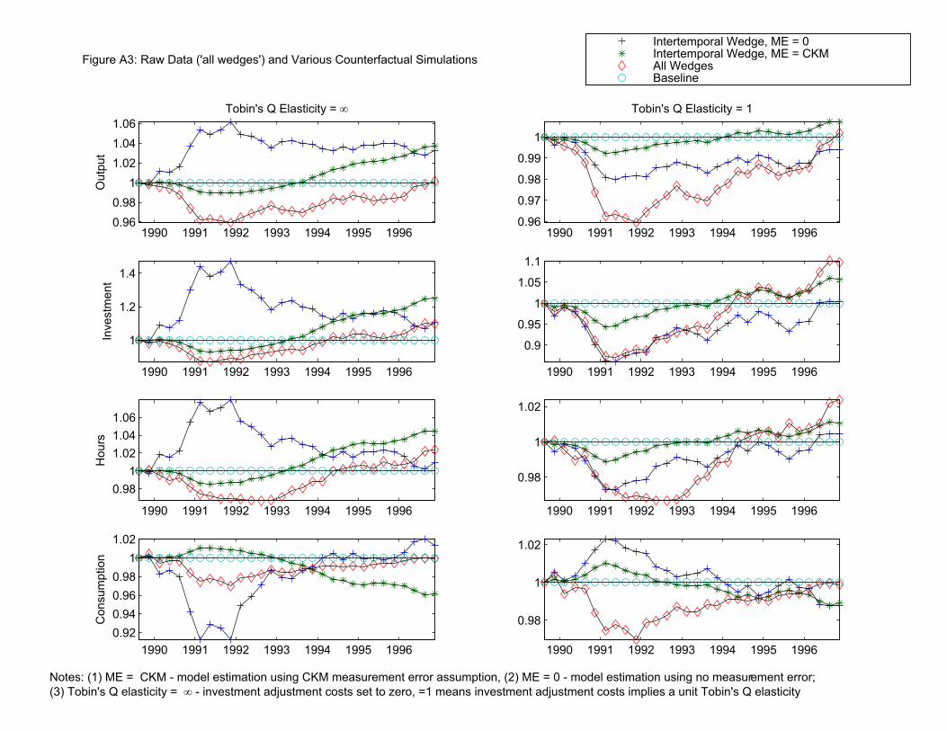
1990 1991 1992 1993 1994 1995 19960.96

0.98

1

1.02

1.04

1.06

Outp

ut

Tobin's Q Elasticity =

1990 1991 1992 1993 1994 1995 1996

1

1.2

1.4

Investm

ent

1990 1991 1992 1993 1994 1995 1996

0.98

1

1.02

1.04

1.06

Hours

1990 1991 1992 1993 1994 1995 1996

0.92

0.94

0.96

0.98

1

1.02

Consum

ption

1990 1991 1992 1993 1994 1995 19960.96

0.97

0.98

0.99

1

Tobin's Q Elasticity = 1

1990 1991 1992 1993 1994 1995 1996

0.9

0.95

1

1.05

1.1

1990 1991 1992 1993 1994 1995 1996

0.98

1

1.02

1990 1991 1992 1993 1994 1995 1996

0.98

1

1.02

Notes: (1) ME = CKM - model estimation using CKM measurement error assumption, (2) ME = 0 - model estimation using no measurement error;

(3) Tobin's Q elasticity = - investment adjustment costs set to zero, =1 means investment adjustment costs implies a unit Tobin's Q elasticity

Figure A3: Raw Data ('all wedges') and Various Counterfactual Simulations

Intertemporal Wedge, ME = 0Intertemporal Wedge, ME = CKMAll WedgesBaseline

2000 2001 2002 2003 20040.95

1

1.05

Outp

ut

Tobin's Q Elasticity =

2000 2001 2002 2003 2004

1

1.2

1.4

Investm

ent

2000 2001 2002 2003 2004

0.95

1

1.05

Hours

2000 2001 2002 2003 2004

0.9

0.95

1

Consum

ption

2000 2001 2002 2003 2004

0.96

0.98

1

Tobin's Q Elasticity = 1

2000 2001 2002 2003 2004

0.9

0.95

1

2000 2001 2002 2003 2004

0.94

0.96

0.98

1

2000 2001 2002 2003 2004

0.99

1

1.01

1.02

Figure A4: Raw Data ('all wedges') and Various Counterfactual Simulations

Notes: (1) ME = CKM - model estimation using CKM measurement error assumption, (2) ME = 0 - model estimation using no measurement error;

(3) Tobin's Q elasticity = - investment adjustment costs set to zero, =1 means investment adjustment costs implies a unit Tobin's Q elasticity

Intertemporal Wedge, ME = 0Intertemporal Wedge, ME = CKMAll WedgesBaseline

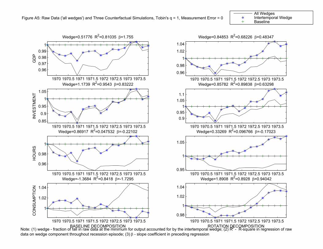
1970 1970.5 1971 1971.5 1972 1972.5 1973 1973.5

0.96

0.97

0.98

0.99

1

Wedge=0.51776 R2=0.81035 =1.755

GD

P

1970 1970.5 1971 1971.5 1972 1972.5 1973 1973.5

0.85

0.9

0.95

1

1.05

Wedge=1.1739 R2=0.9543 =0.83222

INV

ES

TM

EN

T

1970 1970.5 1971 1971.5 1972 1972.5 1973 1973.5

0.96

0.98

1

Wedge=0.86917 R2=0.047532 =-0.22102

HO

UR

S

1970 1970.5 1971 1971.5 1972 1972.5 1973 1973.5

1

1.02

1.04

Wedge=-1.3684 R2=0.8418 =-1.7295

CO

NS

UM

PT

ION

BASELINE DECOMPOSITION

1970 1970.5 1971 1971.5 1972 1972.5 1973 1973.5

0.96

0.98

1

1.02

1.04

Wedge=0.84853 R2=0.68226 =0.48347

1970 1970.5 1971 1971.5 1972 1972.5 1973 1973.5

0.9

0.95

1

1.05

1.1

Wedge=0.85782 R2=0.89838 =0.63298

1970 1970.5 1971 1971.5 1972 1972.5 1973 1973.50.95

1

1.05

Wedge=0.33269 R2=0.096766 =-0.17023

1970 1970.5 1971 1971.5 1972 1972.5 1973 1973.5

0.98

1

1.02

1.04

Wedge=1.8908 R2=0.8928 =0.94042

ROTATION DECOMPOSITION

Figure A5: Raw Data ('all wedges') and Three Counterfactual Simulations, Tobin's q = 1, Measurement Error = 0

Note: (1) wedge - fraction of fall in raw data at the minimum for output accounted for by the intertemporal wedge; (2) R2 - R-square in regression of raw

data on wedge component throughout recession episode; (3) - slope coefficient in preceding regression

All WedgesIntertemporal WedgeBaseline

1974 1975 1976 1977 1978 1979

0.94

0.96

0.98

1

Wedge=0.59855 R2=0.79206 =2.1862

GD

P

1974 1975 1976 1977 1978 1979

0.8

0.9

1

Wedge=1.0623 R2=0.94465 =1.1827

INV

ES

TM

EN

T

1974 1975 1976 1977 1978 19790.94

0.96

0.98

1

Wedge=1.0115 R2=0.71279 =1.2569

HO

UR

S

1974 1975 1976 1977 1978 1979

0.96

0.98

1

1.02

Wedge=-0.64169 R2=0.9046 =-1.4053

CO

NS

UM

PT

ION

BASELINE DECOMPOSITION

1974 1975 1976 1977 1978 1979

0.94

0.96

0.98

1

1.02

Wedge=1.1106 R2=0.87098 =0.65491

1974 1975 1976 1977 1978 1979

0.8

0.9

1

Wedge=0.84323 R2=0.96326 =1.0121

1974 1975 1976 1977 1978 1979

0.95

1

1.05

Wedge=0.62893 R2=0.66166 =0.62529

1974 1975 1976 1977 1978 1979

0.96

0.98

1

1.02

Wedge=1.2428 R2=0.97723 =0.7265

ROTATION DECOMPOSITION

Note: (1) wedge - fraction of fall in raw data at the minimum for output accounted for by the intertemporal wedge; (2) R2 - R-square in regression of raw

data on wedge component throughout recession episode; (3) - slope coefficient in preceding regression

Figure A6: Raw Data ('all wedges') and Three Counterfactual Simulations, Tobin's q = 1, Measurement Error = 0 All WedgesIntertemporal WedgeBaseline

1990 1991 1992 1993 1994 1995 19960.96

0.97

0.98

0.99

1

Wedge=0.5078 R2=0.77707 =1.9646

GD

P

1990 1991 1992 1993 1994 1995 1996

0.9

0.95

1

1.05

1.1Wedge=1.1321 R

2=0.74797 =1.4334

INV

ES

TM

EN

T

1990 1991 1992 1993 1994 1995 1996

0.98

1

1.02

Wedge=0.81405 R2=0.62805 =1.5112

HO

UR

S

1990 1991 1992 1993 1994 1995 1996

0.98

1

1.02

Wedge=-0.5154 R2=0.59606 =-0.72926

CO

NS

UM

PT

ION

BASELINE DECOMPOSITION

1990 1991 1992 1993 1994 1995 19960.96

0.98

1

1.02

1.04

Wedge=0.97262 R2=0.64538 =0.41595

1990 1991 1992 1993 1994 1995 1996

0.9

0.95

1

1.05

1.1Wedge=0.87084 R

2=0.96598 =1.1944

1990 1991 1992 1993 1994 1995 1996

0.98

1

1.02

1.04

1.06

Wedge=0.72304 R2=0.81966 =0.62709

1990 1991 1992 1993 1994 1995 1996

0.98

1

1.02

Wedge=0.97365 R2=0.60399 =0.34821

ROTATION DECOMPOSITION

Figure A7: Raw Data ('all wedges') and Three Counterfactual Simulations, Tobin's q = 1, Measurement Error = 0

Note: (1) wedge - fraction of fall in raw data at the minimum for output accounted for by the intertemporal wedge; (2) R2 - R-square in regression of raw

data on wedge component throughout recession episode; (3) - slope coefficient in preceding regression

All WedgesIntertemporal WedgeBaseline

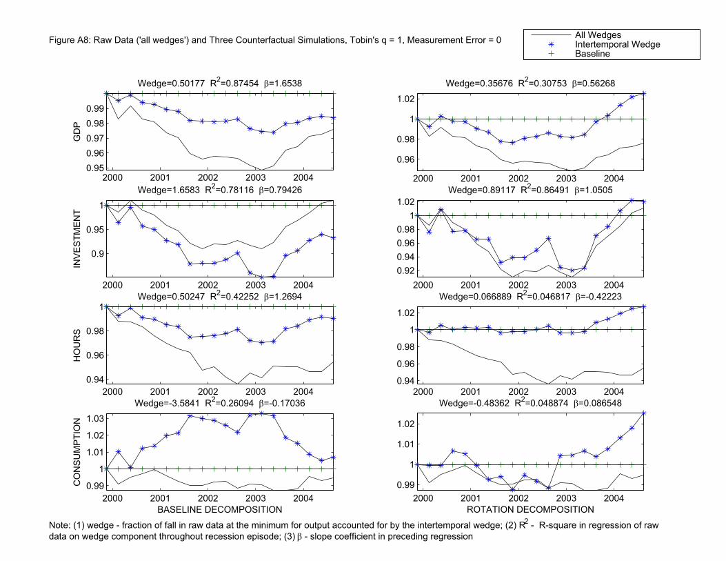
2000 2001 2002 2003 20040.95

0.96

0.97

0.98

0.99

Wedge=0.50177 R2=0.87454 =1.6538

GD

P

2000 2001 2002 2003 2004

0.9

0.95

1

Wedge=1.6583 R2=0.78116 =0.79426

INV

ES

TM

EN

T

2000 2001 2002 2003 2004

0.94

0.96

0.98

1Wedge=0.50247 R

2=0.42252 =1.2694

HO

UR

S

2000 2001 2002 2003 2004

0.99

1

1.01

1.02

1.03

Wedge=-3.5841 R2=0.26094 =-0.17036

CO

NS

UM

PT

ION

BASELINE DECOMPOSITION

2000 2001 2002 2003 2004

0.96

0.98

1

1.02

Wedge=0.35676 R2=0.30753 =0.56268

2000 2001 2002 2003 2004

0.92

0.94

0.96

0.98

1

1.02

Wedge=0.89117 R2=0.86491 =1.0505

2000 2001 2002 2003 2004

0.94

0.96

0.98

1

1.02

Wedge=0.066889 R2=0.046817 =-0.42223

2000 2001 2002 2003 2004

0.99

1

1.01

1.02

Wedge=-0.48362 R2=0.048874 =0.086548

ROTATION DECOMPOSITION

Note: (1) wedge - fraction of fall in raw data at the minimum for output accounted for by the intertemporal wedge; (2) R2 - R-square in regression of raw

data on wedge component throughout recession episode; (3) - slope coefficient in preceding regression

Figure A8: Raw Data ('all wedges') and Three Counterfactual Simulations, Tobin's q = 1, Measurement Error = 0 All WedgesIntertemporal WedgeBaseline

1930 1932 1934 1936 1938 1940

0.7

0.8

0.9

1

Wedge=0.00014874 R2=0.020206 =0.91685

GD

P

1930 1932 1934 1936 1938 1940

0.4

0.6

0.8

1

Wedge=0.00064992 R2=0.23846 =0.95332

INV

ES

TM

EN

T

1930 1932 1934 1936 1938 1940

0.8

0.9

1

Wedge=0.00029434 R2=0.034298 =0.68977

HO

UR

S

1930 1932 1934 1936 1938 1940

0.8

0.9

1

Wedge=-0.00033565 R2=0.10101 =1.3485

CO

NS

UM

PT

ION

BASELINE NONLINEAR DECOMPOSITION

1930 1932 1934 1936 1938 1940

0.7

0.8

0.9

1

Wedge=0.61871 R2=0.79552 =0.98869

1930 1932 1934 1936 1938 1940

0.4

0.6

0.8

1Wedge=0.72082 R

2=0.81247 =1.0121

1930 1932 1934 1936 1938 1940

0.8

0.9

1Wedge=0.75138 R

2=0.74424 =0.99076

Figure A9: Wedges, US Great Depression Based on Second Order Approximation to Model, no Measurement Error, Tobin's q Elasticity = 1

1930 1932 1934 1936 1938 1940

0.8

0.9

1

Wedge=0.54379 R2=0.90475 =1.0033

ROTATION DECOMPOSITION

All WedgesIntertemporal WedgeBaseline

Note: (1) wedge - fraction of fall in raw data at the maximum for output accounted for by the intertemporal wedge; (2) R2 - R-square in regression of raw

data on wedge component throughout recession episode; (3) - slope coefficient in preceding regression.