NBER WORKING PAPER SERIES

WHAT DO WAGE DIFFERENTIALS TELL USABOUT LABOR MARKET DISCRIMINATION?

June E. O’NeillDave M. O’Neill

Working Paper 11240http://www.nber.org/papers/w11240

NATIONAL BUREAU OF ECONOMIC RESEARCH1050 Massachusetts Avenue

Cambridge, MA 02138March 2005

Paper prepared for conference in memory of Tikva Darvish Lecker at Bar-Ilan University, June 27-28, 2004.The authors thank Mei Liao and Wenhui Li for excellent research assistance and participants at theconference for helpful comments. Research support was received from the Olin Foundation. The viewsexpressed herein are those of the author(s) and do not necessarily reflect the views of the National Bureauof Economic Research.

©2005 by June E. O’Neill and Dave M. O’Neill. All rights reserved. Short sections of text, not to exceedtwo paragraphs, may be quoted without explicit permission provided that full credit, including © notice, isgiven to the source.

What Do Wage Differentials Tell Us about Labor Market Discrimination?June E. O’Neill and Dave M. O’NeillNBER Working Paper No. 11240March 2005JEL No. J0

ABSTRACT

We examine the extent to which non-discriminatory factors can explain observed wage gaps between

racial and ethnic minorities and whites, and between women and men. In general we find that

differences in productivity-related factors account for most of the between group wage differences

in the year 2000. Determinants of wage gaps differ by group. Differences in schooling and in skills

developed in the home and in school, as measured by test scores, are of central importance in

explaining black/white and Hispanic/white wage gaps among both women and men. Immigrant

assimilation is an additional factor for Asians and workers from Central and South America. The

sources of the gender gap are quite different, however. Gender differences in schooling and cognitive

skills as measured by the AFQT are quite small and explain little of the pay gap. Instead the gender

gap largely stems from choices made by women and men concerning the amount of time and energy

devoted to a career, as reflected in years of work experience, utilization of part-time work, and other

workplace and job characteristics.

June E. O’NeillCenter for the Study of Business and GovernmentBaruch College, CUNY17 Lexington Avenue - Box C - 406New York, NY 10010and NBERjune_oneill@baruch.cuny.edu

Dave M. O’NeillCenter for the Study of Business and GovernmentBaruch College, CUNY17 Lexington Avenue - Box C - 406New York, NY 10010

1.Introduction With the signing of the Civil Rights Act of 1964, discrimination in employment with

respect to the hiring, promotion and pay of minorities and women became illegal in the

United States.1 Yet, forty years later, earnings differentials still persist between certain

minorities and white non-Hispanics and between women and men. For example, although

the ratio of black men’s earnings to those of white men and of black women’s to white

women’s have increased considerably over the past 50 years, the black-white ratio was

still only 78 percent in 2003 among men and 87 percent among women (Figure 1).

Hispanic-white wage differentials are larger than the black-white differential among both

men and women (Figures 2 and 3). And despite a significant narrowing in the gender gap,

the ratio of women’s earnings to men’s was about 76 percent in 2003 (Figure 4).2

Differentials such as these raise questions in the media and stir the ire of advocacy

groups. However, the existence or absence of a wage gap in itself is not evidence of the

presence of discrimination in the labor market. Groups differ in the extent to which they

have been subject historically to overt discrimination. But groups also differ significantly

in their work-related skills, which alone would create wage differentials. Indeed, some

minorities, such as Asians, earn as much or more than white workers, despite a history of

discrimination.

Our short answer to the question posed in the title of this paper is “not very much”.

We base that conclusion on a detailed empirical analysis of the extent to which

differences in skills and other productivity-related characteristics can explain observed

wage gaps between racial or ethnic minorities and whites and between women and men.

We find that differences in productivity-related factors account for most of the observed

(unadjusted) wage differentials. This is an important finding because the belief that

employment discrimination is the major source of wage differentials can divert attention

away from serious problems generating differentials, such as inadequate schooling.

1 During the 1940s many states outside the South implemented fair employment legislation. For a discussion of the effects see Landes, 1968 and Neumark and Stock, 2001. 2 Figures 1 and 4 depict long-term trends in earnings ratios based on published data from the March Current Population(CPS) reports on median annual earnings of full-time year-round workers. Figures 2 and 3 are based on estimates of mean hourly wage rates derived from the March CPS public use tapes by dividing annual earnings by the product of weeks worked during the year and hours worked per week.

2

In this paper we present the results of our analysis of the sources of racial, ethnic and

gender wage gaps. We start, however, with a brief discussion of economic concepts of

labor market discrimination and their implications for earnings differences between

groups.

2.Economic Concepts of Discrimination

In his seminal work on the economic theory of discrimination Gary Becker (1957)

analyses the effects of employer prejudice on the wages of minorities. An important

implication of Becker’s theory is that competitive markets impose a penalty on a firm in

the form of lower profits when the firm discriminates against workers on the basis of

anything other than productivity differences. Central to the theory is that a prejudiced

employer--in Becker’s terminology, an employer with a “taste” for discrimination --

would only be willing to hire a minority worker at a wage that is less than that of an

equally productive non-minority worker. At any given wage rate for minority workers,

non-discriminating firms will have lower real costs of production than discriminating

firms.

The “taste for discrimination” acts like a tax that firms practicing discrimination

must pay when they hire a minority worker. Non-discriminating firms do not pay this

“tax” and therefore employ larger numbers of minority workers. Although initially they

will be able to employ minorities at wages below the value of their productivity, they will

be willing to pay higher wages (up to the workers’ productivity level). In competitive

markets, the demand for minority workers by employers with no taste for discrimination

can mitigate and eventually even eliminate any earnings effects on minorities.

The extent to which minority wages are ultimately reduced by labor market

discrimination depends on the intensity and distribution of tastes for discrimination

among employers and the interaction of those taste factors with market structure and

production conditions. In situations where a large majority of employers are not

prejudiced, the minority worker population may be able to avoid discrimination.

Moreover, if non-discriminating firms were subject to production conditions that allow

constant or increasing returns to scale, their ability to expand would enable them to drive

out discriminating employers and hire more minority workers. But if non-prejudiced

3

employers (or potential employers) were a minor presence in the market relative to the

size of the minority population, their impact on discrimination in the overall market

would be minimal; and if non-discriminating firms faced decreasing returns to scale, their

potential impact on reducing the effect of discrimination would be further minimized.

Different minorities likely vary in the extent to which they are subject to the effects

of discrimination intensity and its interaction with market/production factors. At one

extreme, the black population at one time was surely exposed to widespread labor market

discrimination. In the pre Civil Rights era, the vast majority of blacks lived in the South

where discriminatory attitudes were prevalent and intense enough to be codified in Jim

Crow laws that restricted the access of the black population to a wide array of public

services, including education, as well as to jobs (Donohue and Heckman, 1991; U.S.

Commission on Civil rights, 1986). Other minorities (for example, Jews and Asians) may

have been able to substantially avoid the effects of labor market discrimination because

they belong to relatively small groups and a sufficient number of employers harbored no

discriminatory feelings towards them.

Becker’s model and those that have developed out of applications of his basic ideas all

focus on the effects of prejudice in the labor market (for example, Black, 1995; Kahn,

1991). However, another class of models of discriminatory outcomes are based on the

premise that employers lack information about the abilities of individual minority and

non-minority workers and assume that individuals will have the average characteristics of

the group to which they belong ( Arrow, 1973; Aigner & Cain, 1977; Lundberg & Startz,

1983; Cain, 1986).

Models of “statistical discrimination” suggest that individual minorities who are

more skilled or productive than the group average can be discriminated against even if

employers are not prejudiced against individual minority members. (Conversely, below-

average majority workers would gain if their group on average were viewed as highly

productive.) Thus a firm might find that the quit rate among its women employees, on

average, was greater than that of men hired for the same job. Faced with the choice

between hiring an individual woman or man of apparently equal qualifications (such as

the same education) it might choose the man based on the premise that the probability of

a woman quitting is higher than that of a man. However, statistical discrimination is

4

likely to diminish as firms find it in their interest to invest in obtaining more information

about the individual workers that they hire (e.g., checking references on prior

employment). Moreover, once workers accumulate a track record at a firm, employers

obtain direct information about individuals on which to base personnel decisions

concerning pay and promotion. Statistical discrimination, like discrimination derived

from prejudice, is prohibited by civil rights legislation. However, in practice it could be

difficult to distinguish between the two.

3. Measuring Discrimination

It is difficult to unravel the role that labor market discrimination plays in earnings

differentials. Direct measures of discrimination are unattainable for national samples of

the population. Individual charges of employer discrimination that are challenged in court

provide little information about the extent of employer discrimination. The vast majority

of such cases are not decided on the merits but on mutual agreement through a consent

decree, which allows the accused firm to avoid potentially large legal and other costs by

payment of a negotiated settlement. In such settlements the employer neither admits to

discrimination nor is found guilty of discrimination by the court.3 In those relatively few

cases that have been decided on the merits, either by a judge or a jury verdict, it is the

employer who has won most of the time (O’Neill and O’Neill, 2005). In any event,

individual instances of discrimination surely exist. But that fact cannot be used to

determine the extent of labor market discrimination or its effects on wages.4

In the absence of direct measures of discrimination researchers investigating the

effect of discrimination on race and gender differences in earnings typically have

addressed a question more amenable to measurement, namely: to what extent can

differences in productivity explain the observed differences? Our ability to determine the

3 Once accused, a firm must mount a costly legal defense and face the bad publicity and possible loss of shareholder and customer support that could result during a lengthy trial, in which the firm’s management is called before the court to confront accusations, baseless or not. A settlement is usually cheaper, especially for large and well known firms, which often are the high profile targets of discrimination suits brought to the Equal Employment Opportunity Commission and federal courts. See the detailed discussion of anti-discrimination cases in Dave M. O’Neill and June O’Neill, “The Federal Government and Job Discrimination” (forthcoming, American Enterprise Institute, 2005) 4 Several studies involving audit experiments

5

answer to this question therefore depends on our ability to measure productivity

differences, never an easy matter.

Because productivity seldom can be observed directly it is necessary to develop

measures of characteristics to serve as proxies for productivity. Survey data vary

considerably in the quality of information provided on the skills of workers, leaving open

the possibility that important aspects of productivity may be omitted from the analysis.

Some basic measures of human capital, such as years of school completed have become

routinely available. However, although differences in years of schooling are an important

source of wage differentials between some groups, it is frequently not the only or even

the main source of wage gaps, and in some cases –such as gender comparisons-- it is not

very important at all. It is difficult to obtain measures of other aspects of skill, such as

actual measures of cognitive development as revealed in test scores or of skills developed

through years of work experience. Among groups with a significant proportion of

immigrants, ability to speak English is important. Rough measures of English language

skill can be obtained from recent census surveys, but other aspects of acculturation are

more difficult to assess.

The measurement pf gender differences in productivity presents a particular

challenge. Labor market outcomes differ between women and men primarily because of

differences in their roles within the family that affect lifetime career paths. Consequently

an analysis of the gender gap in wages requires data on lifetime work experience, and

such data are not routinely included in the major U.S. surveys of work and earnings (for

example, the Current Population Survey or the decennial census). In addition, women’s

continuing family responsibilities can influence their preferences for family-friendly

work situations, leading them to choose jobs that allow for more flexibility and less

commitment of time and effort. Men and women therefore, may make different trade-offs

between pay and job amenities.

In this paper we first examine wage differentials among a large cross-section of

racial and ethnic groups, separately by sex, primarily using the 2000 decennial Census to

obtain large enough samples of small minority groups. We then turn to a series of

analyses based on the National Longitudinal Survey of Youth (NLSY79) which provides

measures of important aspects of work related skills such as test scores and lifetime work

6

experience that are unavailable in the Census data. We analyze the sources of earnings

differentials for the NLSY cohort in 2000 when they had reached ages 35-43 and first

present results for black/white and Hispanic/white differentials separately by sex and than

results for the male-female wage gap.

4. Racial and Ethnic Wage Differentials: Results from the 2000 Census

We start with an overview of the factors influencing the relative wages of various

racial and ethnic groups compared to those of whites using data from the 2000Census.

The analysis is confined to wage and salary workers ages 25-54. The racial/ethnic groups

identified are black non-Hispanics, American Indians, seven groups of Asians

(differentiated by national origin) and seven groups of Hispanics (differentiated by

national origin). Here and throughout the paper whites are always non-Hispanic whites.

Racial and Ethnic Wage Differentials Among Men

We use micro-data from the 2000 Census to conduct OLS log wage regressions

controlling for different sets of explanatory variables. Table 1 shows the log hourly wage

differential between each group and the reference group of white men (given by the

partial regression coefficients on the dummy variables indicating the race/national origin

of each group).

The unadjusted wage differentials (Model 1) vary considerably among the groups.

Japanese, Asian Indian, and Korean men earn about 15% to 25% more than white non-

Hispanic men. Filipino and Chinese men earn 4% to 10% more than white men, while the

group “other Asian” (including Thai, Hmong, Pakistani and Cambodian groups) earn

about 15% less than white men. All of the Hispanic groups earn less than white men and

less than the Asian groups as well.

Mexicans, Dominicans and other Central Americans have the lowest earnings of

any group shown—about half of those of white men. Cubans and Puerto Ricans have the

highest earnings among Hispanics, but still earn about 20% less than white men. Black

and American Indian men earn 25% less than white men. Adjusting for geographic

division and metropolitan/central city location and age (Model 2) reduces some of the

relative advantage of Asian groups because they live in high wage areas.

7

The wage differentials are substantially changed, however, when education

variables are added to the equation (Model 3). Asian groups have very high levels of

education. More than half of Asian men are college graduates or hold higher degrees.

Their earnings advantage is eliminated once education is taken into account. Hispanic

groups, on the other hand, have relatively low levels of schooling. (Almost half of

Hispanic men have not completed high school and only 9% are college graduates.)

Consequently their earnings converge significantly with those of white men when

education variables are added to the model. The Mexican differential is cut in half,

although the change for other Hispanic groups with stronger education backgrounds is

less dramatic. The black-white wage gap, and, even more so the American Indian-white

differential, are also reduced when account is taken of differences in years of schooling.

A relatively large proportion of Asians and Hispanics are migrants. In Model 4 we

add variables indicating years since migrating to the United States and a crude indicator

of English language proficiency (self-reported). The addition of these variables increases

the wages of Hispanics and Asians relative to whites. At this final step, the wages of the

Asian groups are mostly either slightly above or below those of white men, with some

variation. Chinese and the residual group of “other Asian” men earn about 10% less than

white men; Japanese and Vietnamese men earn about 7% more. The gap for Hispanic

men is sharply reduced for all groups but still averages about 10% below that of white

non-Hispanic men. But there is still considerable variation by national origin. The gap for

Dominican men is the highest (19%); the gap for Cuban men is eliminated.

Groups with a significant proportion of migrants present particular difficulties for

analysis because cultural differences among them that influence the speed of assimilation

are only partly captured by measures of schooling and crude self-reported measures of

English speaking ability. Different cohorts of migrants from the same country can differ

because of selection factors. The second generation and earlier generations of immigrants

are likely to be more assimilated. We present additional analysis of Hispanic and black

men below using the superior measures of skills available in the NLSY data.

Racial and Ethnic Wage Differentials Among Women

8

Table 2 replicates for women the analysis of Table 1 and compares the wages of

minority women with those of white non-Hispanic women. Although the patterns of

wage differentials among the different ethnic/racial groups of women are similar to those

of men, the level of the differentials are, for the most part, considerably smaller. Thus the

unadjusted log wage gap between black and white men is –0.273 and between black

women and white women it is -0.112. The wage differentials between white non-

Hispanic women and each group of Hispanic women are also much smaller than they are

for men. After adjusting for schooling, migration and English speaking skills the

differentials among women are further reduced and are mostly on the order of 5% for all

groups except Dominicans and other Central Americans.

The Asian-white differentials are similar for women and men. Asian women, like

Asian men, typically earn more than their white counterparts because of their relatively

high education levels and greater geographic concentration in high wage cities and

regions. Once we control for differences in region, schooling, immigration and language

proficiency, as in Model 4, these positive wage differentials are erased and Asian women

are found to earn about the same wage rate as white women.

6. Black-White and Hispanic-White Earnings Differentials: Results from the NLSY

We turn to the NLSY for a more intensive analysis of the black-white and Hispanic-

white wage gaps among male and among female workers and then in the next section, the

female-male wage gap. The NLSY cohort was first interviewed in 1979 (at ages 14-22)

and was again interviewed each year through 1994 and every other year since then.

Detailed information is provided on lifetime work experience, education and many other

individual characteristics and behaviors of relevance to labor market outcomes. One

unique variable of considerable value is the individual’s score on the Armed Forces

Qualifying Test (AFQT), administered to nearly all survey participants. The test reflects

differences in cognitive skills that are influenced by the quality as well as the quantity of

schooling and by the home environment from early childhood.5

5 Neal and Johnson (1996) find that racial differences in parental education, occupational status and other home background characteristics account for more than 40% of the racial gap in AFQT scores among men in the NLSY. Score differentials emerge at early stages in a child’s development. Hill and O’Neill (1994) in a study of the factors underlying differences in achievement among pre-school children found that more

9

Our NLSY sample is derived from the 2000 survey when the cohort was 35-43 years

of age. The sample includes 5600 wage and salary workers. Blacks and Hispanics were

over-sampled allowing adequate samples for analysis of these groups. Because the cohort

sample was drawn in 1979, the 2000 survey results do not include recent immigrants.

Analysis of the extent to which earnings differences between groups are explained

by differences in characteristics can be executed in several ways. The wage gaps shown

in Tables 1 and 2 are derived from log wage regressions in which a set of dummy (0,1)

variables are used to indicate the race/ethnicity of different groups. The partial regression

coefficients on the dummy variables are interpreted as reflecting the wage differential

between each group and the reference group of white men (or white women in the female

regressions). The underlying assumption is that the effect of relevant characteristics

(other than race/ethnicity) on wages can be approximated by the average effect for all

groups included in the sample.

One issue that arises, however, is the extent to which differences in the effects of

explanatory variables on earnings vary in important ways among groups. For example,

the effect on earnings of an additional year of schooling or of work experience may differ

between blacks and whites. If it is lower for blacks, the question arises whether that

difference reflects employer discrimination. To address that issue we conduct separate

regressions for both blacks and whites, and Hispanics and whites, and present the results

of decomposition analysis based on both sets of partial regression coefficients.

Results for Men

We first show the results of a series of multiple regressions (four models) using the

dummy variable approach to identify log wage differences between groups (Table 3).6

than 40% of the gap in achievement between young black and white children (70% between Hispanic and white children) could be accounted for by differences in measures of family background. Achievement was measured by scores on the Peabody Picture Vocabulary Test ( PPVT ). 6 We again restrict the sample to civilian wage and salary workers, thereby omitting self-employed workers. A comparable wage rate is difficult to estimate for self-employed workers because relevant data on net income, adjusting for capital investment and costs, are not available, and the timing of reported hours worked and of earnings received may not coincide. Moreover, labor market discrimination based on employer behavior is strictly applicable to wage and salary workers, although self-employment income could reflect customer discrimination. We estimate wage rates in the NLSY using the hourly wage as reported directly by those paid by the hour. For those who are paid on another basis—day, week, month, etc., we use usual weekly earnings divided by usual weekly hours. This measure is likely to be a more accurate estimate of the hourly wage than the Census measure which is based on annual earnings during the

10

Separate regressions were run for men of all education levels combined as well as for two

education groups: those with no more than a high school education; and those who are

college graduates or have post college schooling. The highlights are as follows.

Black/white differences: The unadjusted log hourly wage differential was –0.339

between black and white men in 2000 when the NLSY cohort was 35-43 years of age.

Within education group the gaps were smaller (-0.244 for the high school group and –

0.262 for college graduates). The gap is reduced when age and geographic location

variables are included in the regression (model 1). Geographic location makes a

difference because a much larger proportion of black than of white men live in the South

where wages on average are lower for both races. The addition of detailed level of

schooling to the model reduces the gap for all men to –0.186, now similar to that of the

two education groups (model 2).

As shown in Table 4, the mean percentile AFQT score for black men was 24

compared to 55 for white men, and as demonstrated below, AFQT has a large effect on

wages for both blacks and whites. After adding the AFQT percentile score (model 3), the

black–white log wage difference is dramatically reduced: to –0.062 for all men, to-0.075

for the high school group and to –0.05 for college graduates (no longer significant).

These findings (with respect to the explanatory power of the AFQT variable) are similar

to those of Neal and Johnson (1996) and O’Neill (1990) who analyzed the same NLSY

cohort when they were still in their twenties. Neal and Johnson, however, select the

younger portion of the cohort, do not include education and differ in their measurement

of AFQT scores.7

previous calendar year divided by an estimate of annual hours (weeks worked times usual hours per week during the year). Workers were omitted from the NLSY analysis if their reported hourly wage was below $3.50 or more than $125 (in 2000 dollars), a restriction that eliminated 77 men and 81 women (2% of men and 2% of women). Other restrictions included omission of those who did not take the AFQT or who were missing information on key variables or for whom a complete work experience record could not be compiled. Workers were also excluded if they had never been employed during the four-week period prior to the survey interview. We examine the effect of these exclusions below and in the Appendix. 7 The AFQT was administered to the NLSY sample just once—in 1980 when the cohort was 15-23 years of age. Test score results are affected by age and schooling at the time of the test, although the precise effect is difficult to assess because we do not have readings on the AFQT for the same individual at different stages in their lives. We hold constant age and completed education in 2000 in our analyses—an implicit adjustment. Neal and Johnson, 1996 adjust scores for age, but not for education at time of test. O’Neill 1990 holds constant both years of schooling completed at time of test and since the test. We show the

11

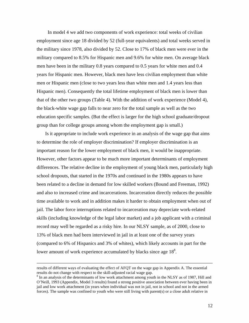
In model 4 we add two components of work experience: total weeks of civilian

employment since age 18 divided by 52 (full-year equivalents) and total weeks served in

the military since 1978, also divided by 52. Close to 17% of black men were ever in the

military compared to 8.5% for Hispanic men and 9.6% for white men. On average black

men have been in the military 0.8 years compared to 0.5 years for white men and 0.4

years for Hispanic men. However, black men have less civilian employment than white

men or Hispanic men (close to two years less than white men and 1.4 years less than

Hispanic men). Consequently the total lifetime employment of black men is lower than

that of the other two groups (Table 4). With the addition of work experience (Model 4),

the black-white wage gap falls to near zero for the total sample as well as the two

education specific samples. (But the effect is larger for the high school graduate/dropout

group than for college groups among whom the employment gap is small.)

Is it appropriate to include work experience in an analysis of the wage gap that aims

to determine the role of employer discrimination? If employer discrimination is an

important reason for the lower employment of black men, it would be inappropriate.

However, other factors appear to be much more important determinants of employment

differences. The relative decline in the employment of young black men, particularly high

school dropouts, that started in the 1970s and continued in the 1980s appears to have

been related to a decline in demand for low skilled workers (Bound and Freeman, 1992)

and also to increased crime and incarcerations. Incarceration directly reduces the possible

time available to work and in addition makes it harder to obtain employment when out of

jail. The labor force interruptions related to incarceration may depreciate work-related

skills (including knowledge of the legal labor market) and a job applicant with a criminal

record may well be regarded as a risky hire. In our NLSY sample, as of 2000, close to

13% of black men had been interviewed in jail in at least one of the survey years

(compared to 6% of Hispanics and 3% of whites), which likely accounts in part for the

lower amount of work experience accumulated by blacks since age 188.

results of different ways of evaluating the effect of AFQT on the wage gap in Appendix A. The essential results do not change with respect to the skill-adjusted racial wage gap. 8 In an analysis of the determinants of low work attachment among youth in the NLSY as of 1987, Hill and O’Neill, 1993 (Appendix, Model 3 results) found a strong positive association between ever having been in jail and low work attachment (in years when individual was not in jail, not in school and not in the armed forces). The sample was confined to youth who were still living with parent(s) or a close adult relative in

12

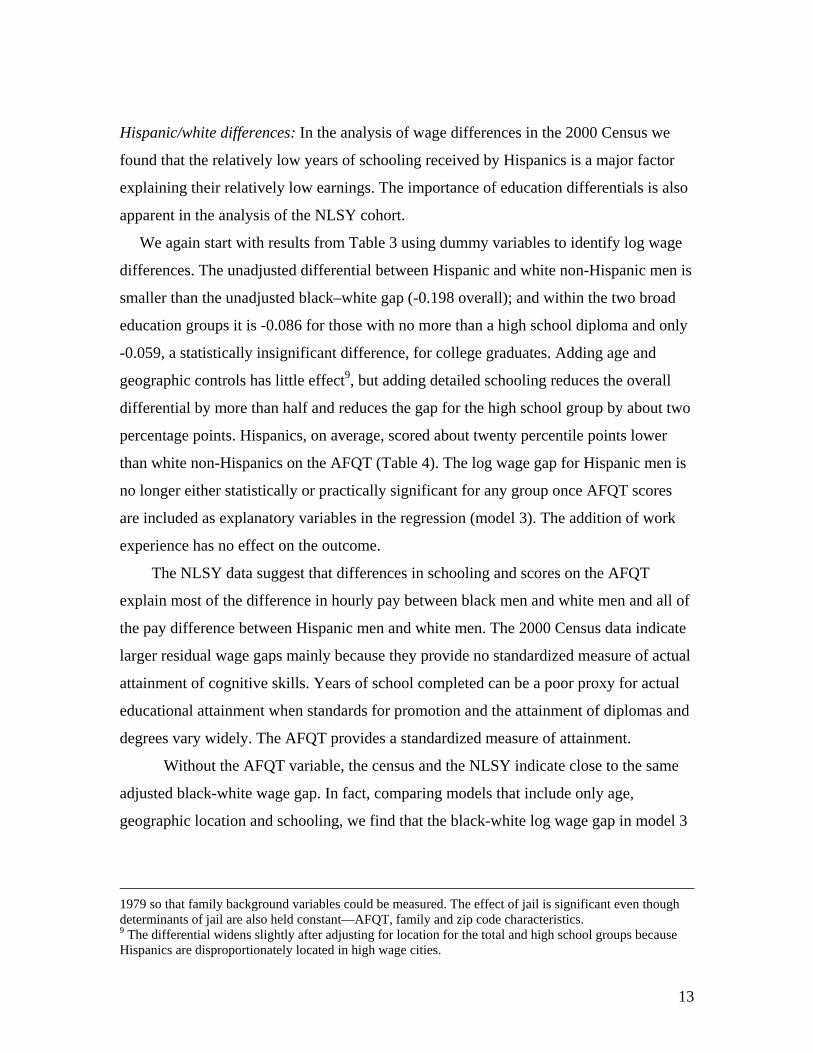
Hispanic/white differences: In the analysis of wage differences in the 2000 Census we

found that the relatively low years of schooling received by Hispanics is a major factor

explaining their relatively low earnings. The importance of education differentials is also

apparent in the analysis of the NLSY cohort.

We again start with results from Table 3 using dummy variables to identify log wage

differences. The unadjusted differential between Hispanic and white non-Hispanic men is

smaller than the unadjusted black–white gap (-0.198 overall); and within the two broad

education groups it is -0.086 for those with no more than a high school diploma and only

-0.059, a statistically insignificant difference, for college graduates. Adding age and

geographic controls has little effect9, but adding detailed schooling reduces the overall

differential by more than half and reduces the gap for the high school group by about two

percentage points. Hispanics, on average, scored about twenty percentile points lower

than white non-Hispanics on the AFQT (Table 4). The log wage gap for Hispanic men is

no longer either statistically or practically significant for any group once AFQT scores

are included as explanatory variables in the regression (model 3). The addition of work

experience has no effect on the outcome.

The NLSY data suggest that differences in schooling and scores on the AFQT

explain most of the difference in hourly pay between black men and white men and all of

the pay difference between Hispanic men and white men. The 2000 Census data indicate

larger residual wage gaps mainly because they provide no standardized measure of actual

attainment of cognitive skills. Years of school completed can be a poor proxy for actual

educational attainment when standards for promotion and the attainment of diplomas and

degrees vary widely. The AFQT provides a standardized measure of attainment.

Without the AFQT variable, the census and the NLSY indicate close to the same

adjusted black-white wage gap. In fact, comparing models that include only age,

geographic location and schooling, we find that the black-white log wage gap in model 3

1979 so that family background variables could be measured. The effect of jail is significant even though determinants of jail are also held constant—AFQT, family and zip code characteristics. 9 The differential widens slightly after adjusting for location for the total and high school groups because Hispanics are disproportionately located in high wage cities.

13

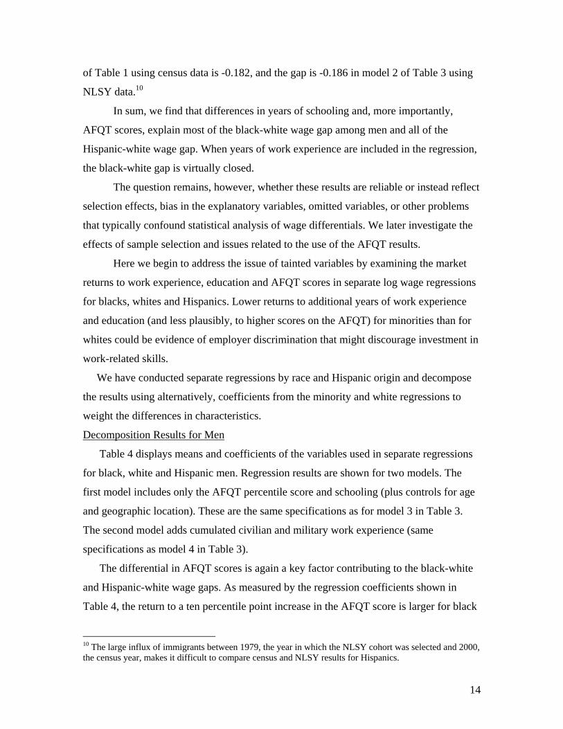
of Table 1 using census data is -0.182, and the gap is -0.186 in model 2 of Table 3 using

NLSY data.10

In sum, we find that differences in years of schooling and, more importantly,

AFQT scores, explain most of the black-white wage gap among men and all of the

Hispanic-white wage gap. When years of work experience are included in the regression,

the black-white gap is virtually closed.

The question remains, however, whether these results are reliable or instead reflect

selection effects, bias in the explanatory variables, omitted variables, or other problems

that typically confound statistical analysis of wage differentials. We later investigate the

effects of sample selection and issues related to the use of the AFQT results.

Here we begin to address the issue of tainted variables by examining the market

returns to work experience, education and AFQT scores in separate log wage regressions

for blacks, whites and Hispanics. Lower returns to additional years of work experience

and education (and less plausibly, to higher scores on the AFQT) for minorities than for

whites could be evidence of employer discrimination that might discourage investment in

work-related skills.

We have conducted separate regressions by race and Hispanic origin and decompose

the results using alternatively, coefficients from the minority and white regressions to

weight the differences in characteristics.

Decomposition Results for Men

Table 4 displays means and coefficients of the variables used in separate regressions

for black, white and Hispanic men. Regression results are shown for two models. The

first model includes only the AFQT percentile score and schooling (plus controls for age

and geographic location). These are the same specifications as for model 3 in Table 3.

The second model adds cumulated civilian and military work experience (same

specifications as model 4 in Table 3).

The differential in AFQT scores is again a key factor contributing to the black-white

and Hispanic-white wage gaps. As measured by the regression coefficients shown in

Table 4, the return to a ten percentile point increase in the AFQT score is larger for black

10 The large influx of immigrants between 1979, the year in which the NLSY cohort was selected and 2000, the census year, makes it difficult to compare census and NLSY results for Hispanics.

14

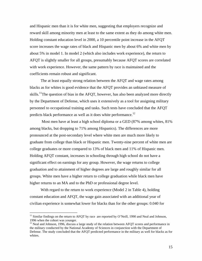
and Hispanic men than it is for white men, suggesting that employers recognize and

reward skill among minority men at least to the same extent as they do among white men.

Holding constant education level in 2000, a 10 percentile point increase in the AFQT

score increases the wage rates of black and Hispanic men by about 6% and white men by

about 5% in model 1. In model 2 (which also includes work experience), the return to

AFQT is slightly smaller for all groups, presumably because AFQT scores are correlated

with work experience. However, the same pattern by race is maintained and the

coefficients remain robust and significant.

The at least equally strong relation between the AFQT and wage rates among

blacks as for whites is good evidence that the AFQT provides an unbiased measure of

skills.11The question of bias in the AFQT, however, has also been analyzed more directly

by the Department of Defense, which uses it extensively as a tool for assigning military

personnel to occupational training and tasks. Such tests have concluded that the AFQT

predicts black performance as well as it does white performance.12

Most men have at least a high school diploma or a GED (87% among whites, 81%

among blacks, but dropping to 71% among Hispanics). The differences are more

pronounced at the post-secondary level where white men are much more likely to

graduate from college than black or Hispanic men. Twenty-nine percent of white men are

college graduates or more compared to 13% of black men and 11% of Hispanic men.

Holding AFQT constant, increases in schooling through high school do not have a

significant effect on earnings for any group. However, the wage returns to college

graduation and to attainment of higher degrees are large and roughly similar for all

groups. White men have a higher return to college graduation while black men have

higher returns to an MA and to the PhD or professional degree level.

With regard to the return to work experience (Model 2 in Table 4), holding

constant education and AFQT, the wage gain associated with an additional year of

civilian experience is somewhat lower for blacks than for the other groups: 0.040 for

11 Similar findings on the return to AFQT by race are reported by O’Neill, 1990 and Neal and Johnson, 1996 when the cohort was younger. 12 Neal and Johnson, 1996, discuss a large study of the relation between AFQT scores and performance in the military conducted by the National Academy of Sciences in conjunction with the Department of Defense. The study concluded that the AFQT predicted performance in the military as well for blacks as for whites.

15

black men, 0.047 for white men and 0.049 for Hispanic men. The return to a year of

military service is lower than the return to a year of civilian work experience for all three

groups.13 The small black-white differences in work experience coefficients may be due

to discontinuities in black male employment. When we add a variable indicating jail time,

the work experience coefficients grow closer (not shown).

The regression decomposition results detailed in Table 5 are based on the

characteristics and regression coefficients for black and white men displayed in Table 4.

Black-white differences in the mean value of each characteristic are weighted

alternatively by the black (or white) regression coefficients from model 1 and model 2

and the weighted differences are then summed to obtain the amount of the wage gap

explained by the particular model and characteristic differences. The same procedure is

followed for the Hispanic-white wage differential.

The results are similar to the results shown in Table 3, which uses the dummy

variable approach to identify the wage effect of race and Hispanic origin. Most or all of

both the black/white wage gap and the Hispanic/white gap are explained by differences in

the basic measures of skill included in Model 1 (AFQT and schooling, plus demographic

controls--age, region, MSA, central city). Moreover, a larger share of the gap is

explained when the minority coefficients are used as the weights. The basic variables

included in Model 1 explain 0.315 of the 0.339 white-black log wage gap when black

coefficients are used as weights, and 0.245 of the gap when white coefficients are used.

The white-Hispanic gap is over-explained with Model 1 specifications using Hispanic

coefficients and almost fully explained when white coefficients are substituted. The

inclusion of work experience in Model 2 raises the explained amount of the white-black

log wage gap and has no effect on the white-Hispanic gap.

Expressed as ratios of hourly wages (the exponentiated log wage gap), the

unadjusted black /white ratio is 71%. The adjusted ratio using black coefficients is 98%

under Model 1 specifications and 102% under Model 2. Using white coefficients, the

adjusted black/white wage ratio is 91% based on Model 1 and 96% under Model 2. The

13 The lower return to military service could reflect simply less relevance of military skills to civilian jobs, since we exclude the active military from our wage sample. However, the subject bears further investigation into the timing of exit from the military and other circumstances of military service. For example, those who recently separated may be experiencing transitional problems.

16

Hispanic/white unadjusted hourly wage ratio is 82%. Adjusted using Hispanic

coefficients it is 103% and using white coefficients it is 98% with no difference between

the models.

Results for Women

Using the NLSY, we conducted similar analyses of the black-white and Hispanic-

white wage gaps for women as for men and the results are displayed in Tables 6-8. Once

again we first ran log wage regressions for all women (and separately for women with

high school educations and women who are college graduates) and use the partial

regression coefficients of dummy variables indicating black race and Hispanic origin to

estimate log wage differentials between these groups and the reference group of white

women.

We present a series of models, each adding new groups of independent variables

(Table 6). In addition to the variables used in our analysis of racial and ethnic differences

among men we include variables that are relevant to women and may have differential

effects by race and Hispanic origin. Because the age of first birth is related to education

and career formation we include a variable indicating if the woman had a first birth

before age 30 and another indicating if she was at least 30 at time of first birth. (Never

had a birth is the omitted category.) We also add to the work experience variables a

measure of the proportion of lifetime weeks worked that were part-time and another that

indicates whether the person ever had a spell out of the labor force due to family

responsibilities.

Similar to the analysis of Census 2000 data, the initial unadjusted log wage gaps

shown in Table 6 are generally smaller for women than for men. The unadjusted log

wage gap for black women (compared to the white non-Hispanic reference group)

is -0.189. However, similar to the pattern for men, the gap falls by half when age,

geographic location and education are included (model 2). When AFQT is also included

(model 3) the gap is eliminated, actually reversing signs to 0.04. The inclusion of fertility

and work experience somewhat raises the positive wage gap (Models 4 and 5). The

pattern of the racial wage gap among women with no more than a high school education

resembles that for all women (second column in Table 6). The pattern for college

17

graduates is also similar through step 4. However, the addition of work experience

widens the gap slightly. But while it remains negative, it is not statistically significant

The unadjusted Hispanic-white log wage gap among women is -0.092. Adding

age, geographic location and schooling reduces the Hispanic-white wage gap for all

education groups combined by two-thirds (model 2 compared to the unadjusted gap). The

remaining differential is statistically insignificant and of insignificant magnitude as well.

The addition of AFQT scores (model 3) reverses the Hispanic–white wage gap for all

Hispanic education groups, including college graduates.

Decomposition Results for Women

Results of a regression decomposition analysis are shown in Table 8 and the

underlying variable means and coefficients from separate regressions for white, black and

Hispanic women are provided in Table 7. The differences in basic skill characteristics

among women by race and ethnicity are similar to those observed among men. Black

women are almost as likely as white women to have completed at least high school (90%

versus 86%) while that percentage for Hispanic women is only 78%. About 28% of white

women completed college, compared to 15% for black women and 14% for Hispanic

women. White women’s mean percentile score on the AFQT is 53% compared to 24%

for black women and 30% for Hispanic women. White women worked somewhat more

weeks since age 18 than black or Hispanic women but white women were much more

likely to have worked part-time. White women were more likely to delay their first birth

to age 30 or more, a decision that is compatible with acquiring additional education and

on-the-job training.

The decomposition results tell approximately the same story as the Table 6 results,

which are based on dummy variables indicating race/Hispanic origin from regressions

including all races. Decomposition results are given for two models, based on the

regression results displayed in Table 7. (Note that Model 1 includes the same variables as

model 3 in Table 6 and Model 2, the same variables as model 6 in Table 6.)

The unadjusted white-black log wage gap among women is 0.189. Model 1, in

addition to age and geographic location, includes only AFQT score and schooling. When

the coefficients from the model 1 regression for black women are used to weight the

mean differences in characteristics, the model implies a higher wage for black women (a

18

gap in favor of black women of 0.1266). The large racial difference in mean scores on the

AFQT test, weighted by the black return to increases in AFQT (which is considerably

larger than the white return) alone explains most of that result. When the white female

regression coefficients are used, the implied wage gap does not reverse, but is negligible:

0.0117. The inclusion of work experience variables in Model 2 barely changes the bottom

line. However, because of the correlation of AFQT and education with work experience,

the net contribution of AFQT and education declines when work experience is added.

Using the Model 2 variables, AFQT still explains more of the white-black wage gap than

any other variable, alone accounting for the whole gap when black coefficients are

employed and half of the gap with white coefficients.

In sum, expressed as hourly wage ratios, the unadjusted black/white ratio for women

is 82.8%. When we control only for differences in education and AFQT (as well as age,

region, MSA, central city) and weight the difference in characteristics with black

women’s coefficients the ratio rises to 113.5%. The ratio rises to about 99% when we

weight with white coefficients. These results are barely changed when we expand the

variables to include work experience and fertility variables (birth before or after age 30,

The unadjusted differential between Hispanic and white women is much smaller—

less than a 10% differential. The differentials in AFQT scores and education between the

two groups more than explain the wage gap, using either the white or Hispanic

coefficients. The unadjusted Hispanic/white hourly wage ratio is 91.2% and rises to

110.7% when we control for AFQT, education and age and location factors using

Hispanic coefficients (103.9% with white coefficients). The inclusion of work experience

and fertility differences has little effect on the adjusted wage ratios.

Overall, the results are quite similar to those for the white-black comparison:

Hispanic women with the same skills as white women would earn four to 10 percent

more than white women, depending on the model and whether Hispanic or white

coefficients are used to weight the differences.

7. The Gender Gap in Wages: Results from the NLSY

19

Measured as the female/male ratio of median annual earnings of all full-time year-

round workers, the gender gap in wages narrowed considerably from the late 1970s when

the ratio was just below 60%, to 2003, when it was 76% (Figure 4). Among the NLSY

cohort, the wage gap in 2000 was 79%, measured as the female /male ratio of hourly

wages (a log wage difference of –0.235, Table 9). Thus, a significant gap in pay remains.

Yet the women and men in the NLSY have similar scores on the AFQT test and about the

same level of schooling.14 Gender differences in wages arise for reasons other than

differences in productivity linked to differences in cognitive skills. Instead, the most

important source of the wage gap is the gender difference in market investments and job

choices that reflect the relative importance of home and market activities in the lives of

women and men.

The division of labor in the family is less delineated than it once was and a majority

of women with children now work in the market. Nonetheless, women on average still

assume greater responsibility for child rearing than men, and that responsibility is

associated with a lower extent and continuity of market work. In addition, the expectation

and assumption of home responsibilities influence choice of occupation and preferences

for working conditions that facilitate a dual career, combining work at home and work in

the market. A significant literature has investigated the effect of work in the home on

women’s lifetime patterns of labor force participation and the effect of labor force

discontinuities on wages.15 Women with children devote relatively more of their energy

to home responsibilities than women without children and as a result earn lower wages.16

On the other hand, married men earn higher wages than other men. Although that effect

may be partly endogenous—women may shun low earners as husbands—it is a plausible

consequence of the division of labor in the home, which leads men to take greater

14 Women have slightly lower scores than men on the AFQT. They are less likely to be high school dropouts, more likely to have 1-3 years of college and about as likely to have college degrees. Men are more likely to have Ph.D’s or professional degrees, but fewer than 2% have such degrees. (See Table 10 for details.) The level of schooling attained by women increased more than that of men over the past two decades and is one of the reasons for the narrowing of the unadjusted gender gap (O’Neill and Polachek, 1993). 15. See Mincer (1962), Mincer and Polachek (1974), and Mincer and Ofek(1982). Also, see Becker (1985) on the effect of home responsibilities on energy in the market. 16 See Walfogel (1995 on the “family gap” in pay. Also see Anderson, Binder and Krause (-) on the “motherhood wage penalty” and see the tables and discussion below.

20

responsibility for providing the family’s money income and consequently to work longer,

more continuously and possibly harder.17

Differences in lifetime work patterns have received considerable attention as a

source of the gender gap. However, another significant source of wage differentials of

particular relevance to the gender gap are the “inequalities arising from the nature of the

employments themselves”.18 As Adam Smith observed, the “agreeableness and

disagreeableness” of employments give rise to equalizing or compensating wage

differences. These non-pecuniary characteristics of employments are likely to be

evaluated differently by women and men. Occupations and individual firms differ in the

extent to which they offer flexible work schedules and a less stressful work environment,

characteristics that are likely to be more highly valued by women. These and other work

amenities are likely to come at a price –i.e., lower wages. Disamenities, such as exposure

to physical hazards, would likely require a premium, other things the same.19 In addition

men and women may differ in their attitudes towards work involving dirty or otherwise

unpleasant physical conditions. Physical differences are likely to affect aptitude for

certain work, for example for jobs requiring heavy lifting, although the proportion of jobs

requiring hard physical labor has declined over time.

It is difficult to estimate the determinants of the gender gap because differences in

standard variables such as years of schooling are not likely to be important sources of the

gap. The NLSY is superior to most other data sets in that it provides more detailed

information than is commonly available on lifetime patterns of work participation as well

as on marriage and family. We create additional proxy variables in an effort to

empirically capture gender differences in choice with respect to employment amenities.

These are described below.

Our analysis of the gender gap follows the same procedures used in our analysis of

racial and ethnic differences. As before, we start with the approach that pools

17 See Becker (1991) on the basic theory of the family. Also see Korenman and Neumark (1991) on the effect of marriage on men’s market productivity. 18 Quoted from Adam Smith , The Wealth of Nations, 1776, Chapter X, Book I. 19 DeLeire and Levy examine the tradeoff between wages and safety and find that married women are much more risk averse than men, requiring a larger compensating differential. They also find that differences in the risk of death at work can account for a significant share of occupational differences by gender.

21

observations of men and women in a single equation and follow with a decomposition

analysis based on separate equations for men and women.

Table 9 shows the effect on the gender gap of controlling for different sets of

explanatory variables from a series of log wage regressions. The wage gap is estimated as

the partial regression coefficient on a dummy variable indicating whether the worker is a

woman. Results are shown for the full sample of male and female workers as well as for

subsets of the sample disaggregated by education and by two polar family status

categories: never had a child and never married and currently married (with or without

own children).

The unadjusted log wage gap for the full sample of men and women is

-0.235. It is essentially unchanged after including education, AFQT and geographic

location. The addition of a vector of three work experience variables, however, reduces

the gender gap by almost half, to -.121 (model 2). The work experience variables include:

weeks worked in civilian jobs since age 18 (converted to years by dividing by 52); weeks

worked in the military divided by 52; and the proportion part-time of total weeks worked

(Table 10). On average, women have worked about two years less than men in military

and civilian jobs combined. Moreover, close to 14% of the weeks worked by women

were part-time compared to 5% for men. Weeks worked have a positive and significant

effect on the hourly wage for both men and women and part-time work has a significant

negative effect for both. However, the magnitude of the effect of part-time on wages is

considerably larger for men than for women (Table 10). The return to years worked,

however, is similar for men and women.

As a proxy for commitment to home responsibilities we add in model 3 a variable

indicating whether the worker had ever withdrawn from the labor force citing child-care

or family responsibilities as the reason. Such labor force withdrawal is associated with an

8% reduction in the wage rate for men as well as women (Table 10). However, 55% of

women and only 13% of men have ever withdrawn because of family responsibilities. As

shown in Table 9, the addition of this variable reduces the gender gap to -0.102.

In model 4 we add two variables indicating whether the person’s job was in

government employment or in the non-profit sector. Non-profit jobs offer more part-time

work and are more likely to allow for flexible schedules and a more relaxed ambience

22

than work in the for-profit sector. As shown in Table 10, women are twice as likely to

work in the non-profit sector than men and employment in the non-profit sector is

associated with lower pay. The effect is significant for women and men but here again the

magnitude of the effect is much larger for men than for women (twice as large).

Government work is also associated with lower pay. However, the effect is weaker and is

not statistically significant for either sex. The addition of the class of worker variables

reduces the gender gap a little-- to -.095.

The final set of variables measure particular characteristics of the 3-digit occupation

held by respondents that are expected to have an effect on wages because they are

associated with on-the-job investment or particular amenities or disamenities. The

occupational characteristics included in our analysis are listed in Table 10 along with the

mean values for men and women separately. Measures of Specific Vocational Preparation

(SVP) and other occupational characteristics were derived from the Dictionary of

Occupational Characteristics (DOT, 1991 version) and from special supplements to the

CPS pertaining to computer use on the job. A variable measuring the level of transition

out of the labor force and another measuring the risk of unemployment in the occupation

were estimated using data from the March CPS.20

The gender gap narrows to -.084 when the occupational characteristics enumerated

in Table 10 are added (model 5). In model 6 we add a variable that measures the percent

female in the respondent’s 3-digit occupation. That addition narrows the gap somewhat

more (to –0.079). Although measures of occupational dissimilarity between men and

women have declined since the 1970s, the occupational distributions of women and men

are still very different (Cavallo and O’Neill, 2004). As shown in Table 10, the women in

our NLSY sample, on average, worked in occupations in which the percent female was

63%; men worked in occupations in which the percent female was 27%. These

occupational differences are sometimes viewed as evidence of discrimination.21

However, the occupations that women choose are strongly predicted by characteristics

20 The data on occupational characteristics were obtained from Cavallo and O’Neill (2004). 21 One school of thought maintains that occupational segregation is the main mechanism through which discrimination is imposed. See the well known work on the crowding hypothesis by Barbara Bergmann (1974).

23

that are compatible with women’s dual careers.22 The percent female in an occupation has

only a limited effect on wages because it is highly correlated with the other occupational

and personal characteristics in the regression. In fact in the log wage regression

based only on the female sample, the percent female is not statistically significant and

bears a positive sign (Table 10). The variable is negative and significant only for the men.

Results in Table 9 are shown for specific sub-groups of the NLSY sample. The results

for the high school group (those with high school diplomas or GED’s or with less

schooling) are similar to those described above for all women and men. However, gender

differences in work experience are more important for the high school group than for all

women and men and account for two-thirds of the wage gap. (Compare the unadjusted

gap with model 2.)

The results for college graduates differ somewhat from those of the other groups.

The unadjusted wage gap is larger, in part because gender differences in skills among

college graduates are somewhat larger. Men are more likely to receive Ph.D’s and

professional degrees and men have higher AFQT scores than women (73rd versus 65th

percentile). Although the gender difference in years worked is slight at the college

graduate level, the difference in part-time work is as large as for the high school group.

Moreover women who are college graduates are less likely to work in the private sector

than other women, or men at any education level. (One-third of female college graduates

work in the non-profit sector and 17% work in government.) A college education appears

to give women access to jobs with working conditions that allow them to work part-time

or to work full-time but under conditions more complementary with care of family such

as the long vacations of teachers. Controlling for both gender differences in class of

worker and occupational characteristics reduces the log wage gap at the college level

from –0.155 (model 3 in Table 9) to -0.078 (model 5). Inclusion of the percent female in

the occupation (model 6) does not affect that result. The gender gap among those with no

more than a high school education is dramatically reduced when we control for work

22 Cavallo and O’Neill (2004) conduct an analysis of the determinants of the percent female in an occupation across three digit occupations and find that variables compatible with women’s constraints (such as the incidence of part-time work and of a long work week and the extent of specific training required) explain most of the variation.

24

experience and is reduced somewhat more when we also include labor force withdrawal

for family reasons, at which point the gap is –0.058 (model 3).

Table 9 (last column) further highlights the relative importance of family

responsibilities versus labor market discrimination by examining the gender gap among

men and women in apparently similar lifetime family situations—namely men and

women who were never married and never had a child. In this case, the unadjusted

gender gap is actually positive—women earn about 8% more than their male

counterparts. This observation is an important one because it suggests that the factors

underlying the gender gap in pay primarily reflect choices made by men and women

given their different societal roles, rather than labor market discrimination against women

due to their sex.

Never-married men and never-married women without children are similar in that

they are not responsible for the financial support of a family as are most married men.

Nor do they have the of responsibility of child care that is usually assumed by women

with children. However, never-married women have better credentials than never-married

men with respect to education, AFQT scores and even years of work experience (Table

11). But never-married men are not notably inferior to other men. In fact, compared to

other men a higher proportion of never-married men are college graduates and they have

about the same AFQT scores. When we control for these differences in characteristics,

the gender gap in favor of women is eliminated, but the negative coefficient is small and

is not statistically significant.

Decomposition Analysis

The comparison of male and female earnings and the interpretation of the gender

gap in pay is further complicated by gender differences in the effects of certain variables

on earnings. As shown in Table 10, in separate wage regressions for women and men the

returns to standard human capital variables such as schooling, years of work experience

and tenure are similar for women and men. However, coefficients differ considerably by

sex when the variable is one that is likely to have a different meaning for women and

men. For example, the variable measuring the proportion of weeks worked part-time

(over the years since the worker was age 22) is negatively associated with earnings for

25

both men and women; but the size of the effect is much larger for men. Also, work for

non-profit employers is negatively associated with earnings for both men and women and

the effect is much stronger for men. And the variable -- percent female in the individual’s

occupation -- is negatively related to earnings for both women and men but the effect for

women is weak and never statistically significant, while the effect for men is usually

larger than the effect for women and significant. (The exception is for male college

graduates for whom the effect of percent female in the occupation is essentially zero.)

How can these findings be explained? Women choose part-time work and non-profit

work because they offer more flexibility and in the case of non-profit firms, less stress.

However, it seems plausible that women working within the private for-profit sector are

more likely to seek job situations that also offer more flexibility although we have no

easy way to detect that with the available data. In that case the difference may be less

stark for women comparing work situations with and without part-time work or in non-

profit versus for-profit firms than would be the case for men. A smaller proportion of

men work part-time than women and those who do are more likely to report that their

part-time work is involuntary, due to inability to find a full time job. But in evaluating the

effect on the wage gap of the gender difference in part-time work or non-profit work

which coefficient should we choose? The effect for men may more nearly reflect the real

trade-off.

Decomposition results for the gender gap using both male and female coefficients are

presented in Table 11 and means and regression coefficients of key variables are given in

Table 10. Because of gender difference in coefficients, such as those noted above, the

results of the decomposition analyses differ depending on whether male or female

coefficients are used. In Table 11, the unadjusted gap, expressed as the ratio of women’s

to men’s hourly wage is 79%. Using male coefficients the ratio rises to 99% when all

variables are included; using female coefficients it rises to 92%.

Which are the more appropriate coefficients to use? The answer depends on

complicated issues related to the degree to which the data we use can accurately measure

differentials in personal and job characteristics. Without better data all we can conclude is

that labor market discrimination is unlikely to account for a differential of more than 8%

and may not be present at all.

26

8. Sample Selection and Other Methodological Issues

Any empirical analysis is subject to error and some researchers have emphasized

possible difficulties that could bias results in analysis of racial and ethnic differentials

(for example, Darity and Mason, 1998) as well as gender differences (Blau, 1998). We

take up the following: Problems in the use of AFQT scores; sample selection;

endogeneity in the human capital variables.

Problems in Using AFQT Scores.

Differentials in AFQT scores reflect both differences in ability and differences in

educational attainment. However, the scores provided in the NLSY data pose difficulties

because the AFQT test was administered only once—in 1980—when the respondents

were ages 15-23, at which time a majority had not completed their schooling. (AFQT

scores arrayed by age and education at the time of test and by education in 2000 are

displayed in Table A-1.) Additional schooling is likely to raise AFQT scores, particularly

for the younger groups. But we have no way of determining by how much it would affect

scores because the correlation of ability and education is not known; nor is the correlation

between ability and AFQT scores. How important a bias this would cause depends on the

strengths of the two correlations. If the ability /score correlation dominates, then our

estimates are not likely to be seriously biased.

The NLSY data allow us to roughly assess the degree of bias in our estimate of

discrimination by using a subset of the data restricted to those who had already completed

their schooling at the time they took the AFQT test. In Appendix Table A-2 (upper panel)

we show the results of a series of log wage regressions on age, location, AFQT, schooling

and work experience, roughly similar to those in Tables 3 and 6.23. We include dummy

variables indicating whether the respondent is black or Hispanic. The table also shows, in

the lower panel, results for the same analysis using all individuals in our NLSY data set,

whether or not they had completed their education at the time of the test. The results

show only a small difference in the coefficients, indicating that the dominant correlation

23 The one difference in the models is that here we use a continuous variable for schooling and in Tables 3 and 6 we use schooling dummies. We use the continuous variable to identify those who had not increased their schooling between 1980 and 2000. However, the non-linear treatment is preferred. The two ways of treating education do produce the small differences in results between Table 3 and Table A-2.

27

is between individual ability ((linked to family background and IQ) and AFQT scores

rather than between educational attainment and AFQT scores. 24

Sample Selection

Our analysis of wage differentials is based on those respondents who were employed

within the last month before the survey interview and reported a wage rate. In addition

we imposed certain restrictions on the sample to remove sources of potential

measurement error and persons missing crucial data. A legitimate question is whether

those omitted from the sample are sufficiently different from those selected to be in the

sample to bias the results. As shown in Appendix Tables A-3 and A-4, out of the entire

cohort of men, 74% of white men were included in our analysis of wage differentials

compared to 68% of black men and 73% of Hispanic men. A somewhat larger proportion

of women were excluded from the analysis. The proportion of women included in the

analysis was 66% for white women, 68% for black women and 63 % for Hispanic

women.

Tables A-3 and A-4 provide information on the characteristics of those included in

the analysis and those excluded. Those who were excluded are grouped into two

categories: those who reported no wage in the last two years, primarily because they were

out of the labor force; and those for whom a wage was reported in the last two years but

were excluded on other grounds. The other grounds for exclusion were : not employed in

the last month, self-employed (our analysis is restricted to wage and salary workers);

AFQT score was missing; wage was below $3.50 or above $125 per hour in 2000. Most

of the excluded men fall into the second category—that is, those for whom a wage was

available. However, among women, those excluded because they had no reported wage in

the last two years were almost as large a group as those who reported wages.

24 Appendix Table A-1 displays scores for men and women by race and Hispanic origin for the NLSY cohort at ages 15-18 and 19-23 at the time of the test and by years of school completed in 1980 and by schooling in 2000. From this table it is possible to get a rough idea of the effect of education, net of ability, for those who had at least some college by 2000, by comparing scores of the older and younger cohort at the same college and college graduate level in 2000. We know all of these people attained the same level of education by 2000. But all of the younger cohort took the test before attending college whereas a substantial portion of the older group had already completed some or more college by 1980. Therefore, the observed test score differential between these two groups provides a rough measure of the net effect of education. The table permits this comparison to be conducted for blacks, whites, and Hispanics, for men and women separately.

28

The data in Table A-3 show that among men the wage rates of those who were

excluded were 73% of those included in our analysis. Moreover, the ratio varies by race.

For whites it was 77%, for blacks 61%, and for Hispanics, 81%. Obviously, the

unadjusted wage gap would be larger if those who were excluded were included in our

analysis.

However, it does not follow that our estimates of the share of the wage gap

attributable to non-discriminatory factors are biased towards minimizing the role of

discrimination because of selection bias. Indeed, those who are excluded from the

analysis generally have productivity related characteristics that would cause them to have

lower earnings than the included group. Moreover, the skill gaps between the included

and excluded groups are greater for minorities than for whites. For example, as indicated

in table A-3, the differentials between those included and those excluded from the

analysis with respect to AFQT scores, years worked since age 18 and percent ever in jail,

are significantly greater among black and Hispanic men than among white men.

Therefore, it does not necessarily follow that the inclusion of these men in the analysis

would alter our findings about the share of the wage gap due to non-discriminatory

factors. (Table A-4 indicates similar comparisons between minority and white women

and points to the same conclusion.)

In order to get some idea of the potential effect of selection bias we have estimated

our basic regression model including all the excluded respondents for whom we had

wage data within the past two years. (We still exclude those with no AFQT reported

because of the key role of that variable in explaining the differential.) This analysis has

important limitations because the excluded group was excluded because their reported

wages are both less current and less reliable. The results are shown in Tables A-5 for men

and A-6 for women and can be compared with our basic analysis in Tables 3 and 6.

The only significant finding of the expanded analysis is that our estimate of the male

black/white wage gap possibly attributable to discrimination could be raised from

practically zero (the result in Table 3) to 5% (the result in Table A-5). The expanded

analysis does not significantly change our estimates of the Hispanic/white wage gap for

men or our estimates of the black/white or Hispanic/white wage gap among women.

29

One explanation for the larger gap for black men in the expanded analysis is that

black men who were excluded from our basic analysis have had much higher

incarceration rates over their lifetimes than either Hispanic or white males, and much

higher incarceration rates than black men included in our basic sample. As indicated in

Table A-3, 29% of black men who were excluded from our basic analysis but were

included in our expanded analysis were interviewed in jail or in prison in at least one of

the NLSY surveys, compared to 7% of white men and 18% of Hispanic men. Among

black men who reported no wage during the past two years, 44% had ever been in jail. As

discussed above, criminal activity is strongly associated with reduced employment, even

during periods when not in jail (Bound and Freeman, 1992; Hill and O’Neill, 1993). A

history of incarceration has been shown to contribute to earnings loss and decreased wage

growth over the life-cycle (Western, 2002; Holzer, Offner and Sorenson, 2004). We did

not incorporate the effects of incarceration into our analysis, although this would be a

good future project.25

Selection issues are often raised with respect to the gender gap because a larger

percentage of women than of men are out of the labor force. Among the NLSY cohort,

34% of women and 28% of men were excluded from our basic analysis. (Compare Tables

A-3 and A-4.) Of this group, 54% of women and 70% of men reported a wage within the

past two years. The female/male wage ratio for this excluded group is slightly lower than

it is for those in our basic analysis (77% versus 79%). The women excluded from the

basic analysis have characteristics linked to lower wage rates---in particular, almost three

years less work experience, a larger proportion reporting withdrawal from the labor force

due to family responsibilities, and more part-time work. Schooling and AFQT scores are

only slightly lower.

We have estimated the gender wage gap using the regression sequence shown in

Table 9, for an expanded sample including all those women and men who were excluded

from our basic analysis but reported a wage within the past two years. The results (Table

25 We have included a measure of lifetime work experience, which is clearly associated with incarceration. However, a full treatment would require detail on the timing and length of labor force interruptions and the effect of these interruptions on wage growth. The problem is a kin to that addressed by Mincer and Polachek in studying women’s labor force interruptions.

30

A-7) are highly similar to those of Table 9—a gender wage gap of –0.067 with the

expanded sample compared to -0.079 with the basic sample.

In sum, the unadjusted measure of the wage gap for the various groups we have

compared would be somewhat larger in each case if we could include those without an

observed wage. However, in each case, with the exception of the male black/white wage

gap, the wage gap adjusted for differentials in productivity does not change significantly

when we include a substantial proportion of those who were initially excluded. Thus

sample selection does not appear to be concealing evidence of discrimination. Although

we did not attempt to estimate the effect of including those who had no wage rate within

the past two years, an inspection of their characteristics suggests that their inclusion

would likely widen the unadjusted wage gap but also might not have any significant

effect on the adjusted gap.

Endogeneity Issues

In any analysis of cause and effect involving natural or uncontrolled experimental

situations, the question arises whether the explanatory variables in the model are

themselves affected by labor market discrimination. In particular, the question is often

raised whether educational attainment, test scores and other factors are themselves

affected by labor market discrimination against minorities and women.

The argument is sometimes made that the lower educational attainment and test

scores of blacks compared to whites can be attributed in part to their anticipation that

they will earn a lower return on their investment because of discrimination in the labor

market. Thus studies that regress earnings on educational attainment and test scores to

help explain the racial earnings gap will tend to underestimate the effects of labor market

discrimination on earnings because some of the lower attainment of blacks is itself due to

labor market discrimination. However, the evidence from our analysis and those of

others, suggests that when log wage regressions are run separately for blacks and whites

the partial regression coefficients of the test score and educational attainment variables do

not differ significantly, suggesting the same rate of return. It was once true that the

returns to education for blacks were lower than for whites (U.S. Commission on Civil

Rights, 1986). However, the return to college education has been higher for blacks than

for whites since the 1970s (Heckman, 1998). Moreover, the gap in educational attainment

31

between blacks and whites has converged sharply over the years, suggesting that blacks

have been reacting to increased incentives.

As we demonstrate above, the market return to higher AFQT scores is actually

somewhat higher for blacks than to whites. Moreover, as discussed above, the AFQT has

been tested extensively and found to be free of cultural bias.

Years of schooling and AFQT scores largely reflect characteristics and skills

developed outside the market and are not likely to be affected by current labor market

discrimination. In the early decades of the twentieth century most blacks lived in the

South, where Jim Crow laws and regulations limited employment opportunities, and

societal discrimination reinforced by state and local policies severely restricted their

access to education (U.S. Commission on Civil Rights, 1986; Smith, 1984, Welch, 1973).

Racial discrimination in publicly provided school resources was eventually eliminated

and there has been significant convergence in the black-white gap in years of schooling

completed. Nonetheless, the legacy of educational deprivation may have a lingering

effect on the early acquisition of skills through low parental education and income.26

However, differences in skills that stem from a disadvantaged family background are

quite distinct from employer discrimination.

Work experience obviously can be directly influenced by labor market

discrimination. But it is an empirical question whether that is in fact the case. We have

earlier discussed the issue in the context of the lower lifetime work experience of black

men and noted that the relative decline in the employment of less educated black men,

that began in the 1970s has been shown to be related to the decline in demand for low-

skilled workers and to their increased involvement in crime and resulting imprisonment.

There is no good evidence that we know of suggesting that labor market discrimination is

greater now than it was in the 1940s through the 1960s when the employment of black

men was relatively higher than it has become.27

In the analysis of the gender gap, issues of bias in the explanatory variables have been

raised with respect to both work experience and occupation. Women’s employment rates

have increased so rapidly over the past several decades that allegations that labor market

26 See footnote 5 above. 27 The US Commission on Civil Rights (1986) provides data showing the relatively sharp decline in black male employment after 1960 that occurred despite advances in education and earnings.

32

discrimination is reducing women’s labor force participation per se have little force.

However, the issue is still raised with respect to occupational differences. We believe that

gender differences in occupation and type of job reflect choice, not employer prejudices.

Our analysis indicates that women choose occupations and job settings that are

compatible with combining market and home work. It would be difficult to find an

explanation based on employer choice that could explain the observed patterns.

9. Concluding Comments

Differences in the quantity of education as measured by years of schooling, and the

amount and quality of skill developed in the home and in school, as measured by test

scores, are of central importance in explaining the black/white and Hispanic/white wage

gaps among women as well as among men in the labor force. Schooling and immigrant

status are particularly relevant in explaining wage differences between whites and groups

such as Asians (many of whom earn more than whites) and individuals from Central and

South America. Our analysis of the factors underlying the black/white wage gap leads us

to concur with the conclusion reached by James Heckman (1998) that “most of the

disparity in earnings between blacks and whites in the labor market of the 1990s is due to

the differences in the skills they bring to the market, and not to discrimination in the

market.” The same conclusion can be applied in 2000 to other racial and ethnic

comparisons.

The gender gap is more difficult to analyze because the reasons for the difference are

harder to measure. Gender differences in schooling and cognitive skills as measured by

the AFQT are quite small and explain little of the pay gap. Instead the gender gap is

attributable to choices made by women concerning the amount of time and energy to

devote to a career as reflected in years of work experience, utilization of part-time work,

and workplace and job characteristics. There is no gender gap in wages among men and

women with similar family roles. Comparing the wage gap between women and men

ages 35-43 who have never married and never had a child, we find a small observed gap

in favor of women, which becomes insignificant after accounting for differences in skills

and job and workplace characteristics. What the average woman sacrifices in earnings

from choosing jobs that allow for part-time work and flexible work conditions is

presumably offset by a gain in the utility of time spent with children and family.

33

REFERENCES Aigner, Dennis J. and Glen Cain, “Statistical Theories of Discrimination in Labor Economics”, Industrial Labor Relations Review 30 (Dec., 1986): 175-87. Anderson, D., M. Binder and K.Krause, “The Motherhood Wage Penalty Revisited: Experience, Heterogeneity, Work Effort, and Work Schedule Flexibility”, Industrial and Labor Relations Review, Vol. 56, No. 2, (2003). Arrow, Kenneth J., “The Theory of Discrimination”. In Discrimination in the Labor Market, edited by Orley Ashenfelter and Albert Rees. Princeton, NJ: Princeton University Press, 1973. Becker, Gary S., The Economics of Discrimination. Chicago : University of Chicago Press. (1957) Becker, Gary S. A Treatise on the Family. Cambridge, Mass: Harvard University Press, 1981. Becker, Gary S,. “Human Capital, Effort, and the Sexual Division of Labor”, Journal of Labor Economics, 3:1 Pt.2, pp s33-s58 (1988) Black, Dan A., ”Discrimination in an Equilibrium Search Model”, Journal of Labor Economics, Vol. 13, No. 2, (1995): 309-34 Blau, Francine D., “Trends in the Well-Being of American Women, 1970-1995,” Journal of Economic Literature 36 (March 1998): 112-165. Bound, John and Richard B. Freeman. "What Went Wrong? The Erosion of Relative Earnings and Employment among Young Black Men in the 1980s." Quarterly Journal of Economics 107 (February 1992): 201-23 Cain, Glen G., The Economic Analysis of Labor Market Discrimination: A Survey. Handbook of Labor Economics, Vol. 1, edited by Orley Ashenfelter and Richard Layard. Amsterdam: North Holland (1986) Cavallo, Alex and June O’Neill, “Determinants of the Gender Gap in Occupations and Earnings”, Paper presented at the meetings of the Society of Labor Economists, San Antonio, May 2004 Darity, William A. and Patrick L. Mason, “Evidence on Discrimination in Employment: Codes of Color, Codes of Gender”, Journal of Economic Perspectives, Vol.12, No.2 (Spring, 1998), 63-90. DeLeire, Thomas and Helen Levy, “Worker Sorting and the Risk of Death on the Job”

34

Journal of Labor Economics, 2004 Donahue, John and James Heckman, “Continuous vs. Episodic Change: The Impact of Affirmative Action and Civil Rights Policy on the Economic Status of Blacks,” Journal of Economic Literature, December 1991, 29:4, 1603-43. Heckman James, “Detecting Discrimination” Journal of Economic Perspectives, 12:2 pp 101-16, (1998) Hill, M. Anne and June O’Neill, “Intercohort Change in Women’s Labor Market Status”, Research in Labor Economics,vol 13, edited by R.G. Ehrenberg, Greenwich, Conn: JAI, (1992) Hill, M. Anne and June O’Neill. “Family Endowments and the Achievement of Young Children with Special Reference to the Underclass.” Journal of Human Resources 29, no.4 (Fall 1994): 1064-1101. Hill, M. Anne and June O’Neill, Underclass Behaviors in the United States: Measurement and Analysis of Determinants, Center for the Study of Business and Government, Baruch College, CUNY (Revised August, 1993) Holzer, Harry, Paul Offner, and Elaine Sorenson. Declining employment among black less-educated men: The role of incarceration and child support. Unpublished paper, The Urban Institute, Washington, DC (2004) Kahn, Lawrence M., “Customer Discrimination and Affirmative Action”, Economic Inquiry 29 (July, 1991): 555-71. Korenman, Sanders and David Neumark, “ Does Marriage Really Make men more Productive?”, Journal of Human Resources, 1991, 26:2, 282-307. Landes, William, “The Economics of Fair Employment Laws”, Journal of Political Economy, vol 76, pp 507-52, (1968) Lundberg, Shelly J. & Startz, R., Private Discrimination and Social Intervention in Competitive Labor Markets, American Economic Review 73 (June, 1983): 340-47. Mincer, Jacob, “Labor Force Participation of Married Women: A Study of Labor Supply”, in Aspects of Labor Economics, edited by C. Christ, Princeton, N.J., Princeton University Press, (1962) Mincer, and Polachek, “Family Investments in Human Capital: Earnings of Women”, Journal of Political Economy, 82, pp S76-S108, (1974) Mincer and Ofek, “Interrupted Work Careers: Depreciation and Restoration of Human Capital”, Journal of Human Resources, 17, No 1, pp 3-24, (1982)

35

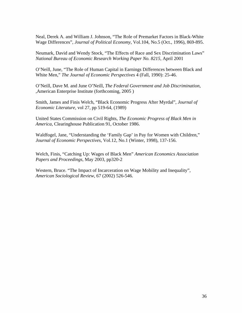
Neal, Derek A. and William J. Johnson, “The Role of Premarket Factors in Black-White Wage Differences”, Journal of Political Economy, Vol.104, No.5 (Oct., 1996), 869-895. Neumark, David and Wendy Stock, “The Effects of Race and Sex Discrimination Laws” National Bureau of Economic Research Working Paper No. 8215, April 2001 O’Neill, June, “The Role of Human Capital in Earnings Differences between Black and White Men,” The Journal of Economic Perspectives 4 (Fall, 1990): 25-46. O’Neill, Dave M. and June O’Neill, The Federal Government and Job Discrimination, ,American Enterprise Institute (forthcoming, 2005 ) Smith, James and Finis Welch, “Black Economic Progress After Myrdal”, Journal of Economic Literature, vol 27, pp 519-64, (1989) United States Commission on Civil Rights, The Economic Progress of Black Men in America, Clearinghouse Publication 91, October 1986. Waldfogel, Jane, “Understanding the ‘Family Gap’ in Pay for Women with Children,” Journal of Economic Perspectives, Vol.12, No.1 (Winter, 1998), 137-156.

Welch, Finis, “Catching Up: Wages of Black Men” American Economics Association Papers and Proceedings, May 2003, pp320-2 Western, Bruce. “The Impact of Incarceration on Wage Mobility and Inequality”, American Sociological Review, 67 (2002) 526-546.

36

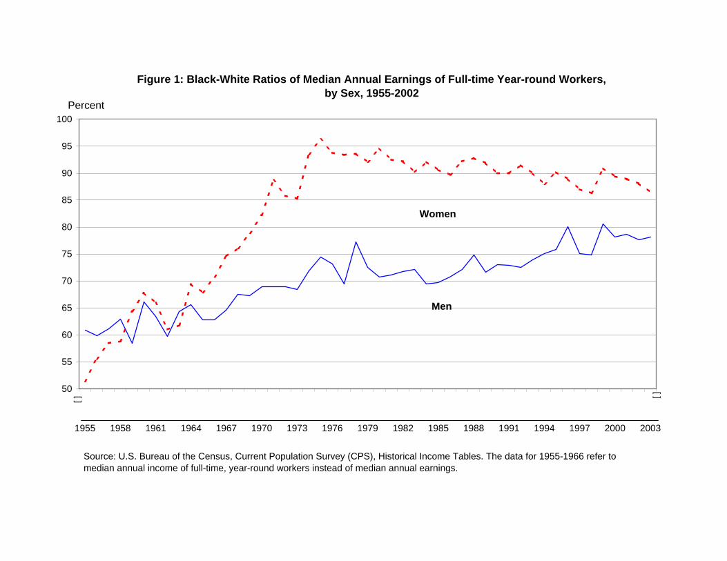
Figure 1: Black-White Ratios of Median Annual Earnings of Full-time Year-round Workers, by Sex, 1955-2002

50

55

60

65

70

75

80

85

90

95

100

1955 1958 1961 1964 1967 1970 1973 1976 1979 1982 1985 1988 1991 1994 1997 2000 2003

Percent

[ ] [ ]

Source: U.S. Bureau of the Census, Current Population Survey (CPS), Historical Income Tables. The data for 1955-1966 refer to median annual income of full-time, year-round workers instead of median annual earnings.

Women

Men

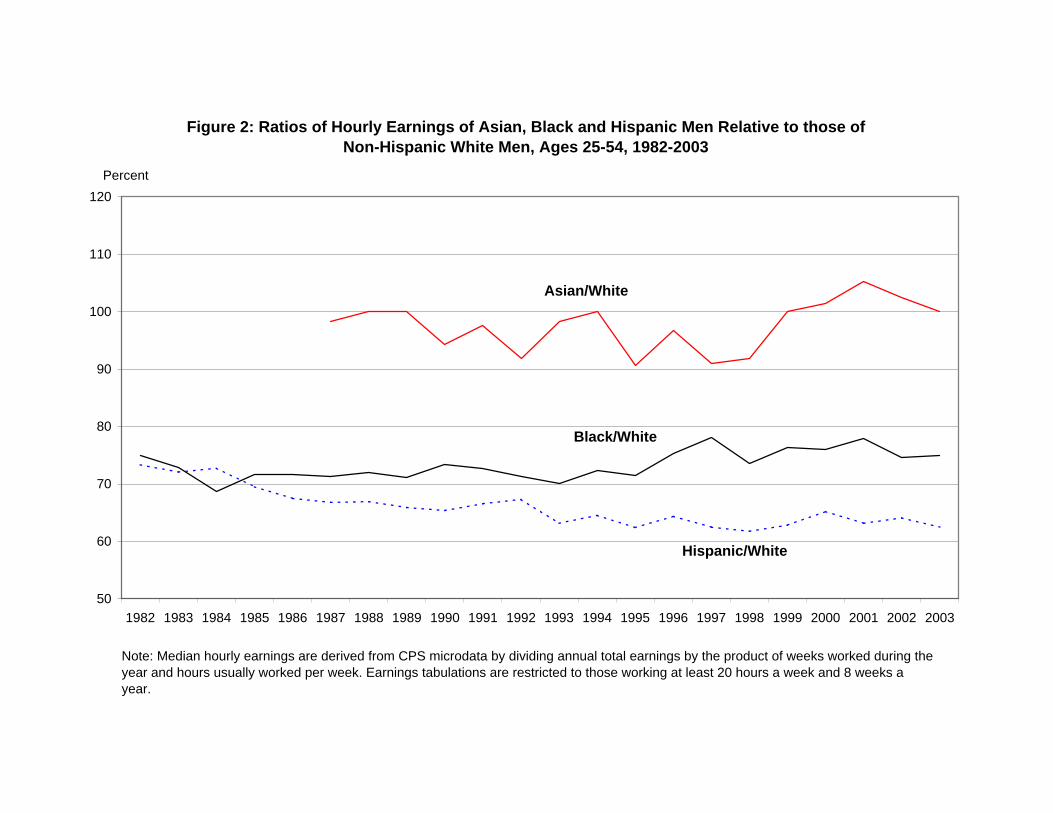
Figure 2: Ratios of Hourly Earnings of Asian, Black and Hispanic Men Relative to those of Non-Hispanic White Men, Ages 25-54, 1982-2003

50

60

70

80

90

100

110

120

1982 1983 1984 1985 1986 1987 1988 1989 1990 1991 1992 1993 1994 1995 1996 1997 1998 1999 2000 2001 2002 2003

Note: Median hourly earnings are derived from CPS microdata by dividing annual total earnings by the product of weeks worked during the year and hours usually worked per week. Earnings tabulations are restricted to those working at least 20 hours a week and 8 weeks a year.

Asian/White

Black/White

Hispanic/White

Percent

Figure 3: Ratios of Hourly Earnings of Asian, Black and Hispanic Relative to those of Non-Hispanic White Women, Ages 25-54, 1982-2003

50

60

70

80

90

100

110

120

1982 1983 1984 1985 1986 1987 1988 1989 1990 1991 1992 1993 1994 1995 1996 1997 1998 1999 2000 2001 2002 2003

Percent

Note: Median hourly earnings are derived from CPS microdata by dividing annual total earnings by the product of weeks worked during the year and hours usually worked per week. Earnings tabulations are restricted to those working at least 20 hours a week and 8 weeks a year.

Asian/White

Black/White

Hispanic/White

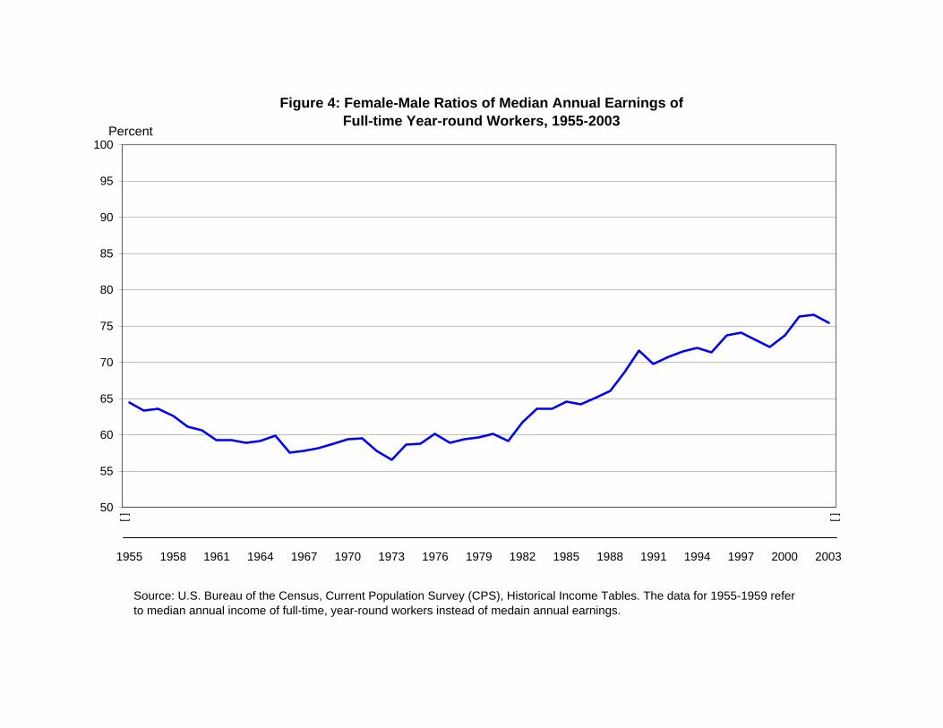
Figure 4: Female-Male Ratios of Median Annual Earnings of Full-time Year-round Workers, 1955-2003

50

55

60

65

70

75

80

85

90

95

100

1955 1958 1961 1964 1967 1970 1973 1976 1979 1982 1985 1988 1991 1994 1997 2000 2003

Percent[ ] [ ]

Source: U.S. Bureau of the Census, Current Population Survey (CPS), Historical Income Tables. The data for 1955-1959 refer to median annual income of full-time, year-round workers instead of medain annual earnings.

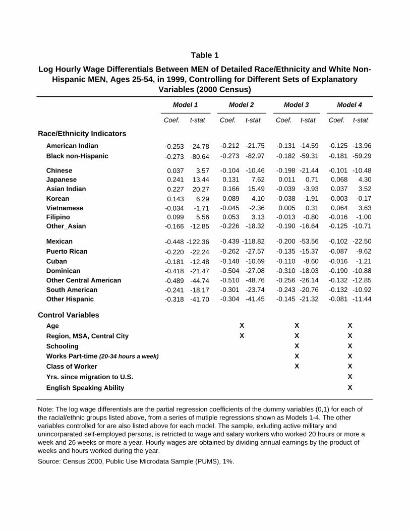
Table 1

Log Hourly Wage Differentials Between MEN of Detailed Race/Ethnicity and White Non-Hispanic MEN, Ages 25-54, in 1999, Controlling for Different Sets of Explanatory

Variables (2000 Census)

Model 1 Model 2 Model 3 Model 4

Coef. t-stat Coef. t-stat Coef. t-stat Coef. t-stat

Race/Ethnicity IndicatorsAmerican Indian -0.253 -24.78 -0.212 -21.75 -0.131 -14.59 -0.125 -13.96Black non-Hispanic -0.273 -80.64 -0.273 -82.97 -0.182 -59.31 -0.181 -59.29

Chinese 0.037 3.57 -0.104 -10.46 -0.198 -21.44 -0.101 -10.48Japanese 0.241 13.44 0.131 7.62 0.011 0.71 0.068 4.30Asian Indian 0.227 20.27 0.166 15.49 -0.039 -3.93 0.037 3.52Korean 0.143 6.29 0.089 4.10 -0.038 -1.91 -0.003 -0.17Vietnamese -0.034 -1.71 -0.045 -2.36 0.005 0.31 0.064 3.63Filipino 0.099 5.56 0.053 3.13 -0.013 -0.80 -0.016 -1.00Other_Asian -0.166 -12.85 -0.226 -18.32 -0.190 -16.64 -0.125 -10.71

Mexican -0.448 -122.36 -0.439 -118.82 -0.200 -53.56 -0.102 -22.50Puerto Rican -0.220 -22.24 -0.262 -27.57 -0.135 -15.37 -0.087 -9.62Cuban -0.181 -12.48 -0.148 -10.69 -0.110 -8.60 -0.016 -1.21Dominican -0.418 -21.47 -0.504 -27.08 -0.310 -18.03 -0.190 -10.88Other Central American -0.489 -44.74 -0.510 -48.76 -0.256 -26.14 -0.132 -12.85South American -0.241 -18.17 -0.301 -23.74 -0.243 -20.76 -0.132 -10.92Other Hispanic -0.318 -41.70 -0.304 -41.45 -0.145 -21.32 -0.081 -11.44

Control VariablesAge X X XRegion, MSA, Central City X X XSchooling X XWorks Part-time (20-34 hours a week) X XClass of Worker X XYrs. since migration to U.S. XEnglish Speaking Ability X

Note: The log wage differentials are the partial regression coefficients of the dummy variables (0,1) for each of the racial/ethnic groups listed above, from a series of mutiple regressions shown as Models 1-4. The other variables controlled for are also listed above for each model. The sample, exluding active military and unincorparated self-employed persons, is retricted to wage and salary workers who worked 20 hours or more a week and 26 weeks or more a year. Hourly wages are obtained by dividing annual earnings by the product of weeks and hours worked during the year. Source: Census 2000, Public Use Microdata Sample (PUMS), 1%.

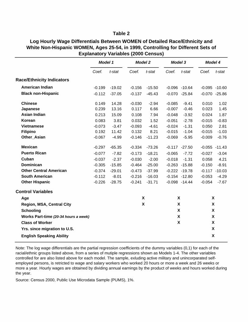
Table 2Log Hourly Wage Differentials Between WOMEN of Detailed Race/Ethnicity and

White Non-Hispanic WOMEN, Ages 25-54, in 1999, Controlling for Different Sets of Explanatory Variables (2000 Census)

Model 1 Model 2 Model 3 Model 4

Coef. t-stat Coef. t-stat Coef. t-stat Coef. t-stat

Race/Ethnicity IndicatorsAmerican Indian -0.199 -19.02 -0.156 -15.50 -0.096 -10.64 -0.095 -10.60Black non-Hispanic -0.112 -37.05 -0.137 -45.43 -0.070 -25.84 -0.070 -25.86

Chinese 0.149 14.28 -0.030 -2.94 -0.085 -9.41 0.010 1.02Japanese 0.239 13.16 0.117 6.66 -0.007 -0.46 0.023 1.45Asian Indian 0.213 15.09 0.108 7.94 -0.048 -3.92 0.024 1.87Korean 0.083 3.81 0.032 1.52 -0.051 -2.78 -0.015 -0.83Vietnamese -0.073 -3.47 -0.093 -4.61 -0.024 -1.31 0.050 2.81Filipino 0.192 11.42 0.132 8.21 -0.015 -1.04 -0.015 -1.03Other_Asian -0.067 -4.99 -0.146 -11.23 -0.069 -5.95 -0.009 -0.76

Mexican -0.297 -65.35 -0.334 -73.26 -0.117 -27.50 -0.055 -11.43Puerto Rican -0.077 -7.82 -0.173 -18.21 -0.065 -7.72 -0.027 -3.04Cuban -0.037 -2.37 -0.030 -2.00 -0.018 -1.31 0.058 4.21Dominican -0.305 -15.85 -0.464 -25.00 -0.263 -15.88 -0.150 -8.91Other Central American -0.374 -29.01 -0.473 -37.99 -0.222 -19.78 -0.117 -10.03South American -0.112 -8.01 -0.216 -16.03 -0.154 -12.80 -0.053 -4.29Other Hispanic -0.226 -28.75 -0.241 -31.71 -0.098 -14.44 -0.054 -7.67

Control VariablesAge X X XRegion, MSA, Central City X X XSchooling X XWorks Part-time (20-34 hours a week) X XClass of Worker X XYrs. since migration to U.S. X

English Speaking Ability X

Note: The log wage differentials are the partial regression coefficients of the dummy variables (0,1) for each of the racial/ethnic groups listed above, from a series of mutiple regressions shown as Models 1-4. The other variables controlled for are also listed above for each model. The sample, exluding active military and unincorparated self-employed persons, is retricted to wage and salary workers who worked 20 hours or more a week and 26 weeks or more a year. Hourly wages are obtained by dividing annual earnings by the product of weeks and hours worked during the year.

Source: Census 2000, Public Use Microdata Sample (PUMS), 1%.

*

*

*

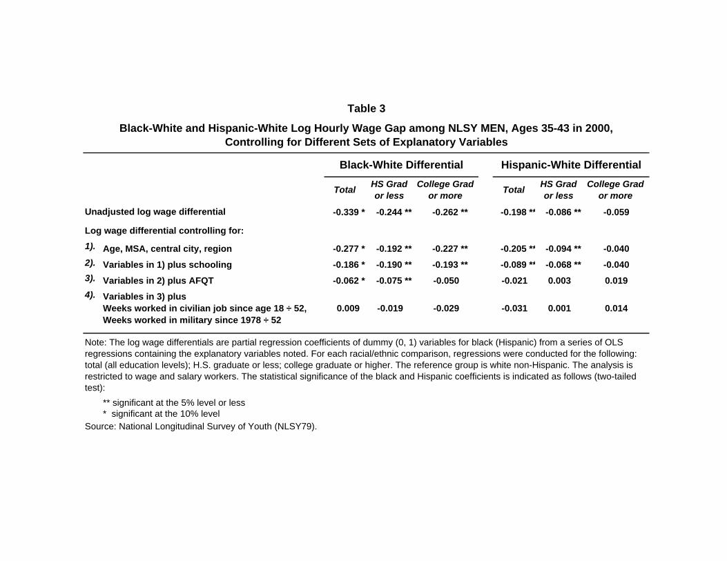
Table 3

Black-White and Hispanic-White Log Hourly Wage Gap among NLSY MEN, Ages 35-43 in 2000, Controlling for Different Sets of Explanatory Variables

Black-White Differential Hispanic-White Differential

Total HS Grad or less

College Grad or more Total HS Grad

or lessCollege Grad

or more

Unadjusted log wage differential -0.339 ** -0.244 ** -0.262 ** -0.198 * -0.086 ** -0.059

Log wage differential controlling for:1). Age, MSA, central city, region -0.277 ** -0.192 ** -0.227 ** -0.205 * -0.094 ** -0.0402). Variables in 1) plus schooling -0.186 ** -0.190 ** -0.193 ** -0.089 * -0.068 ** -0.0403). Variables in 2) plus AFQT -0.062 ** -0.075 ** -0.050 -0.021 0.003 0.0194). Variables in 3) plus

Weeks worked in civilian job since age 18 ÷ 52, Weeks worked in military since 1978 ÷ 52

0.009 -0.019 -0.029 -0.031 0.001 0.014

Note: The log wage differentials are partial regression coefficients of dummy (0, 1) variables for black (Hispanic) from a series of OLS regressions containing the explanatory variables noted. For each racial/ethnic comparison, regressions were conducted for the following: total (all education levels); H.S. graduate or less; college graduate or higher. The reference group is white non-Hispanic. The analysis is restricted to wage and salary workers. The statistical significance of the black and Hispanic coefficients is indicated as follows (two-tailed test):

** significant at the 5% level or less* significant at the 10% level

Source: National Longitudinal Survey of Youth (NLSY79).

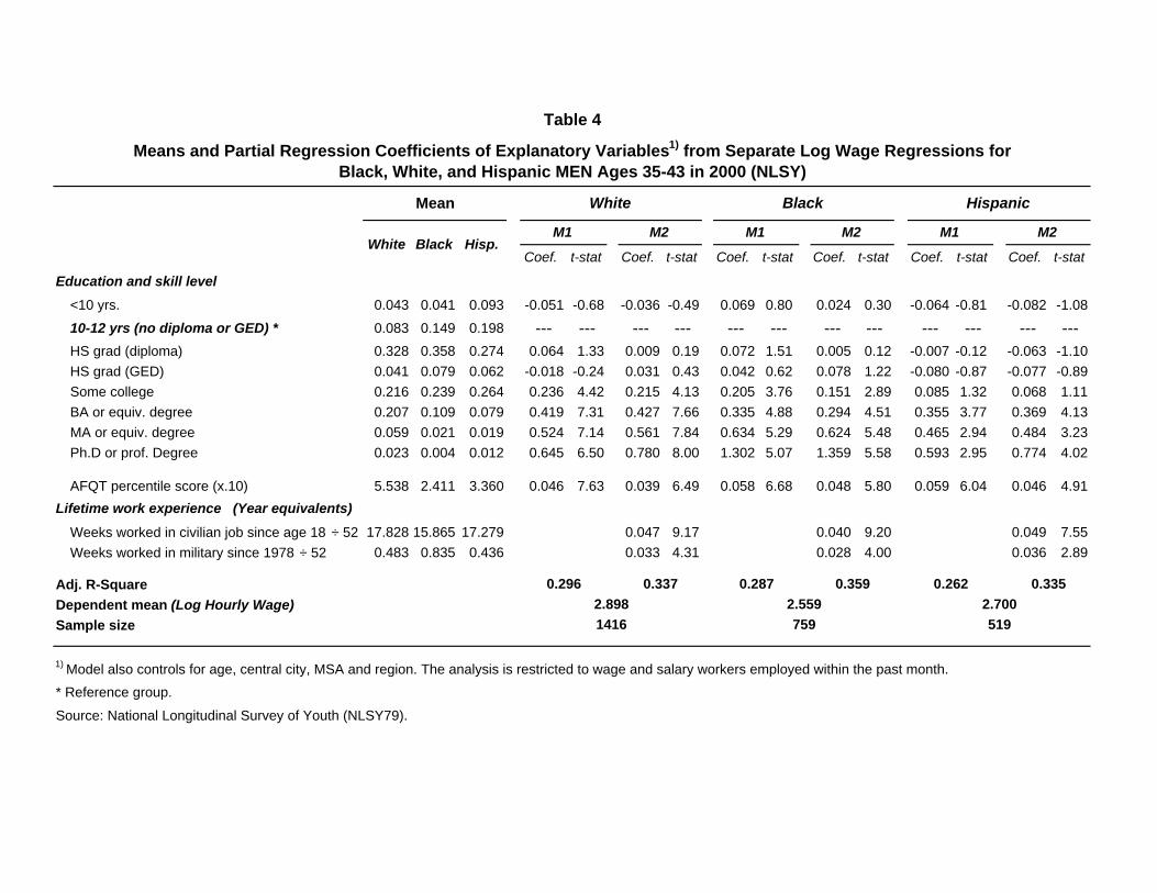
Table 4

Means and Partial Regression Coefficients of Explanatory Variables1) from Separate Log Wage Regressions for Black, White, and Hispanic MEN Ages 35-43 in 2000 (NLSY)

Mean White Black Hispanic

White Black Hisp.M1 M2 M1 M2 M1 M2

Coef. t-stat Coef. t-stat Coef. t-stat Coef. t-stat Coef. t-stat Coef. t-stat

Education and skill level<10 yrs. 0.043 0.041 0.093 -0.051 -0.68 -0.036 -0.49 0.069 0.80 0.024 0.30 -0.064 -0.81 -0.082 -1.08

10-12 yrs (no diploma or GED) * 0.083 0.149 0.198 --- --- --- --- --- --- --- --- --- --- --- ---HS grad (diploma) 0.328 0.358 0.274 0.064 1.33 0.009 0.19 0.072 1.51 0.005 0.12 -0.007 -0.12 -0.063 -1.10HS grad (GED) 0.041 0.079 0.062 -0.018 -0.24 0.031 0.43 0.042 0.62 0.078 1.22 -0.080 -0.87 -0.077 -0.89Some college 0.216 0.239 0.264 0.236 4.42 0.215 4.13 0.205 3.76 0.151 2.89 0.085 1.32 0.068 1.11BA or equiv. degree 0.207 0.109 0.079 0.419 7.31 0.427 7.66 0.335 4.88 0.294 4.51 0.355 3.77 0.369 4.13MA or equiv. degree 0.059 0.021 0.019 0.524 7.14 0.561 7.84 0.634 5.29 0.624 5.48 0.465 2.94 0.484 3.23Ph.D or prof. Degree 0.023 0.004 0.012 0.645 6.50 0.780 8.00 1.302 5.07 1.359 5.58 0.593 2.95 0.774 4.02

AFQT percentile score (x.10) 5.538 2.411 3.360 0.046 7.63 0.039 6.49 0.058 6.68 0.048 5.80 0.059 6.04 0.046 4.91Lifetime work experience (Year equivalents)

Weeks worked in civilian job since age 18 ÷ 52 17.828 15.865 17.279 0.047 9.17 0.040 9.20 0.049 7.55Weeks worked in military since 1978 ÷ 52 0.483 0.835 0.436 0.033 4.31 0.028 4.00 0.036 2.89

Adj. R-Square 0.296 0.337 0.287 0.359 0.262 0.335Dependent mean (Log Hourly Wage) 2.898 2.559 2.700Sample size 1416 759 519

1) Model also controls for age, central city, MSA and region. The analysis is restricted to wage and salary workers employed within the past month. * Reference group.

Source: National Longitudinal Survey of Youth (NLSY79).

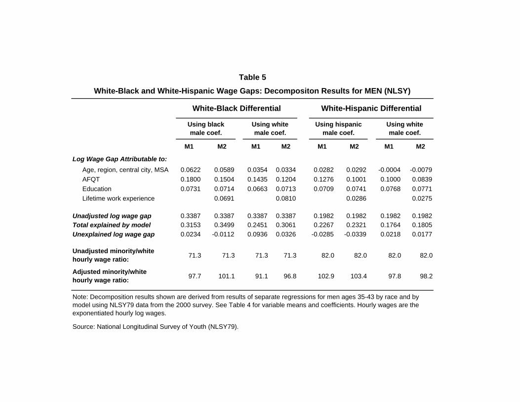
Table 5White-Black and White-Hispanic Wage Gaps: Decompositon Results for MEN (NLSY)

White-Black Differential White-Hispanic Differential

Using black male coef.

Using white male coef.

Using hispanic male coef.

Using white male coef.

M1 M2 M1 M2 M1 M2 M1 M2

Log Wage Gap Attributable to:Age, region, central city, MSA 0.0622 0.0589 0.0354 0.0334 0.0282 0.0292 -0.0004 -0.0079AFQT 0.1800 0.1504 0.1435 0.1204 0.1276 0.1001 0.1000 0.0839Education 0.0731 0.0714 0.0663 0.0713 0.0709 0.0741 0.0768 0.0771Lifetime work experience 0.0691 0.0810 0.0286 0.0275

Unadjusted log wage gap 0.3387 0.3387 0.3387 0.3387 0.1982 0.1982 0.1982 0.1982Total explained by model 0.3153 0.3499 0.2451 0.3061 0.2267 0.2321 0.1764 0.1805Unexplained log wage gap 0.0234 -0.0112 0.0936 0.0326 -0.0285 -0.0339 0.0218 0.0177

Unadjusted minority/white hourly wage ratio: 71.3 71.3 71.3 71.3 82.0 82.0 82.0 82.0

Adjusted minority/white hourly wage ratio: 97.7 101.1 91.1 96.8 102.9 103.4 97.8 98.2

Note: Decomposition results shown are derived from results of separate regressions for men ages 35-43 by race and by model using NLSY79 data from the 2000 survey. See Table 4 for variable means and coefficients. Hourly wages are the exponentiated hourly log wages.

Source: National Longitudinal Survey of Youth (NLSY79).

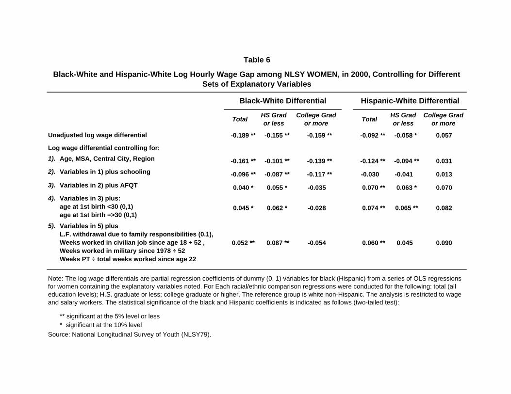
Table 6

Black-White and Hispanic-White Log Hourly Wage Gap among NLSY WOMEN, in 2000, Controlling for Different Sets of Explanatory Variables

Black-White Differential Hispanic-White Differential

Total HS Grad or less

College Grad or more Total HS Grad

or lessCollege Grad

or more

Unadjusted log wage differential -0.189 ** -0.155 ** -0.159 ** -0.092 ** -0.058 * 0.057

Log wage differential controlling for:1). Age, MSA, Central City, Region -0.161 ** -0.101 ** -0.139 ** -0.124 ** -0.094 ** 0.0312). Variables in 1) plus schooling -0.096 ** -0.087 ** -0.117 ** -0.030 -0.041 0.0133). Variables in 2) plus AFQT 0.040 * 0.055 * -0.035 0.070 ** 0.063 * 0.0704). Variables in 3) plus:

age at 1st birth <30 (0,1) age at 1st birth =>30 (0,1)

0.045 * 0.062 * -0.028 0.074 ** 0.065 ** 0.082

5). Variables in 5) plus L.F. withdrawal due to family responsibilities (0.1), Weeks worked in civilian job since age 18 ÷ 52 , Weeks worked in military since 1978 ÷ 52 Weeks PT ÷ total weeks worked since age 22

0.052 ** 0.087 ** -0.054 0.060 ** 0.045 0.090

Note: The log wage differentials are partial regression coefficients of dummy (0, 1) variables for black (Hispanic) from a series of OLS regressions for women containing the explanatory variables noted. For Each racial/ethnic comparison regressions were conducted for the following: total (all education levels); H.S. graduate or less; college graduate or higher. The reference group is white non-Hispanic. The analysis is restricted to wage and salary workers. The statistical significance of the black and Hispanic coefficients is indicated as follows (two-tailed test):

** significant at the 5% level or less* significant at the 10% level

Source: National Longitudinal Survey of Youth (NLSY79).

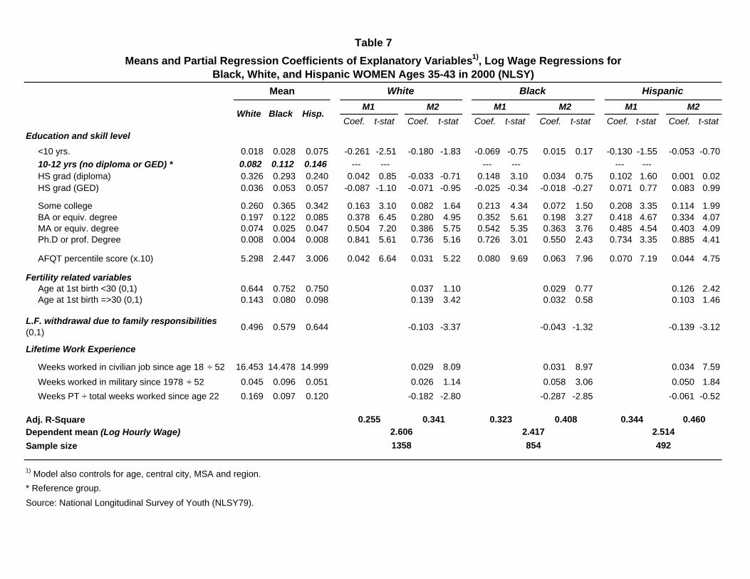
Table 7Means and Partial Regression Coefficients of Explanatory Variables1), Log Wage Regressions for

Black, White, and Hispanic WOMEN Ages 35-43 in 2000 (NLSY)

Mean White Black Hispanic

White Black Hisp.M1 M2 M1 M2 M1 M2

Coef. t-stat Coef. t-stat Coef. t-stat Coef. t-stat Coef. t-stat Coef. t-statEducation and skill level

<10 yrs. 0.018 0.028 0.075 -0.261 -2.51 -0.180 -1.83 -0.069 -0.75 0.015 0.17 -0.130 -1.55 -0.053 -0.7010-12 yrs (no diploma or GED) * 0.082 0.112 0.146 --- --- --- --- --- ---HS grad (diploma) 0.326 0.293 0.240 0.042 0.85 -0.033 -0.71 0.148 3.10 0.034 0.75 0.102 1.60 0.001 0.02HS grad (GED) 0.036 0.053 0.057 -0.087 -1.10 -0.071 -0.95 -0.025 -0.34 -0.018 -0.27 0.071 0.77 0.083 0.99

Some college 0.260 0.365 0.342 0.163 3.10 0.082 1.64 0.213 4.34 0.072 1.50 0.208 3.35 0.114 1.99BA or equiv. degree 0.197 0.122 0.085 0.378 6.45 0.280 4.95 0.352 5.61 0.198 3.27 0.418 4.67 0.334 4.07MA or equiv. degree 0.074 0.025 0.047 0.504 7.20 0.386 5.75 0.542 5.35 0.363 3.76 0.485 4.54 0.403 4.09Ph.D or prof. Degree 0.008 0.004 0.008 0.841 5.61 0.736 5.16 0.726 3.01 0.550 2.43 0.734 3.35 0.885 4.41

AFQT percentile score (x.10) 5.298 2.447 3.006 0.042 6.64 0.031 5.22 0.080 9.69 0.063 7.96 0.070 7.19 0.044 4.75

Fertility related variablesAge at 1st birth <30 (0,1) 0.644 0.752 0.750 0.037 1.10 0.029 0.77 0.126 2.42Age at 1st birth =>30 (0,1) 0.143 0.080 0.098 0.139 3.42 0.032 0.58 0.103 1.46

L.F. withdrawal due to family responsibilities (0,1) 0.496 0.579 0.644 -0.103 -3.37 -0.043 -1.32 -0.139 -3.12

Lifetime Work Experience

Weeks worked in civilian job since age 18 ÷ 52 16.453 14.478 14.999 0.029 8.09 0.031 8.97 0.034 7.59

Weeks worked in military since 1978 ÷ 52 0.045 0.096 0.051 0.026 1.14 0.058 3.06 0.050 1.84Weeks PT ÷ total weeks worked since age 22 0.169 0.097 0.120 -0.182 -2.80 -0.287 -2.85 -0.061 -0.52

Adj. R-Square 0.255 0.341 0.323 0.408 0.344 0.460Dependent mean (Log Hourly Wage) 2.606 2.417 2.514Sample size 1358 854 492

1) Model also controls for age, central city, MSA and region. * Reference group.Source: National Longitudinal Survey of Youth (NLSY79).

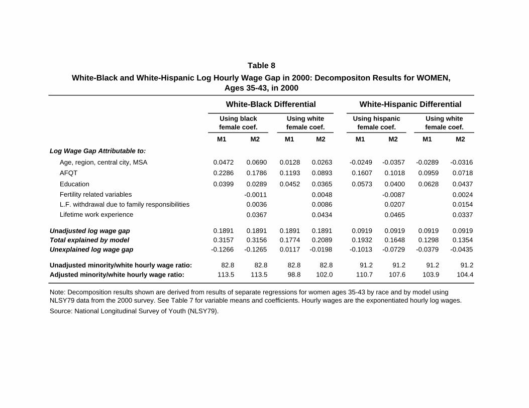
Table 8White-Black and White-Hispanic Log Hourly Wage Gap in 2000: Decompositon Results for WOMEN,

Ages 35-43, in 2000

White-Black Differential White-Hispanic DifferentialUsing black female coef.

Using white female coef.

Using hispanic female coef.

Using white female coef.

M1 M2 M1 M2 M1 M2 M1 M2

Log Wage Gap Attributable to:Age, region, central city, MSA 0.0472 0.0690 0.0128 0.0263 -0.0249 -0.0357 -0.0289 -0.0316AFQT 0.2286 0.1786 0.1193 0.0893 0.1607 0.1018 0.0959 0.0718

Education 0.0399 0.0289 0.0452 0.0365 0.0573 0.0400 0.0628 0.0437Fertility related variables -0.0011 0.0048 -0.0087 0.0024L.F. withdrawal due to family responsibilities 0.0036 0.0086 0.0207 0.0154Lifetime work experience 0.0367 0.0434 0.0465 0.0337

Unadjusted log wage gap 0.1891 0.1891 0.1891 0.1891 0.0919 0.0919 0.0919 0.0919Total explained by model 0.3157 0.3156 0.1774 0.2089 0.1932 0.1648 0.1298 0.1354Unexplained log wage gap -0.1266 -0.1265 0.0117 -0.0198 -0.1013 -0.0729 -0.0379 -0.0435

Unadjusted minority/white hourly wage ratio: 82.8 82.8 82.8 82.8 91.2 91.2 91.2 91.2Adjusted minority/white hourly wage ratio: 113.5 113.5 98.8 102.0 110.7 107.6 103.9 104.4

Note: Decomposition results shown are derived from results of separate regressions for women ages 35-43 by race and by model using NLSY79 data from the 2000 survey. See Table 7 for variable means and coefficients. Hourly wages are the exponentiated hourly log wages. Source: National Longitudinal Survey of Youth (NLSY79).

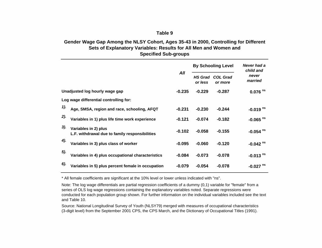
Table 9

Gender Wage Gap Among the NLSY Cohort, Ages 35-43 in 2000, Controlling for Different Sets of Explanatory Variables: Results for All Men and Women and

Specified Sub-groups

AllBy Schooling Level Never had a

child and never

marriedHS Grad or less

COL Grad or more

Unadjusted log hourly wage gap -0.235 -0.229 -0.287 0.076 ns

Log wage differential controlling for:

1). Age, SMSA, region and race, schooling, AFQT -0.231 -0.230 -0.244 -0.019 ns

2). Variables in 1) plus life time work experience -0.121 -0.074 -0.182 -0.065 ns

3). Variables in 2) plus L.F. withdrawal due to family responsibilities -0.102 -0.058 -0.155 -0.054 ns

4).Variables in 3) plus class of worker -0.095 -0.060 -0.120 -0.042 ns

5).Variables in 4) plus occupational characteristics -0.084 -0.073 -0.078 -0.013 ns

6). Variables in 5) plus percent female in occupation -0.079 -0.054 -0.078 -0.027 ns

* All female coefficients are significant at the 10% level or lower unless indicated with "ns".

Note: The log wage differentials are partial regression coefficients of a dummy (0,1) variable for "female" from a series of OLS log wage regressions containing the explanatory variables noted. Separate regressions were conducted for each population group shown. For further information on the individual variables included see the text and Table 10.Source: National Longitudinal Survey of Youth (NLSY79) merged with measures of occupational characteristics (3-digit level) from the September 2001 CPS, the CPS March, and the Dictionary of Occupational Titles (1991).

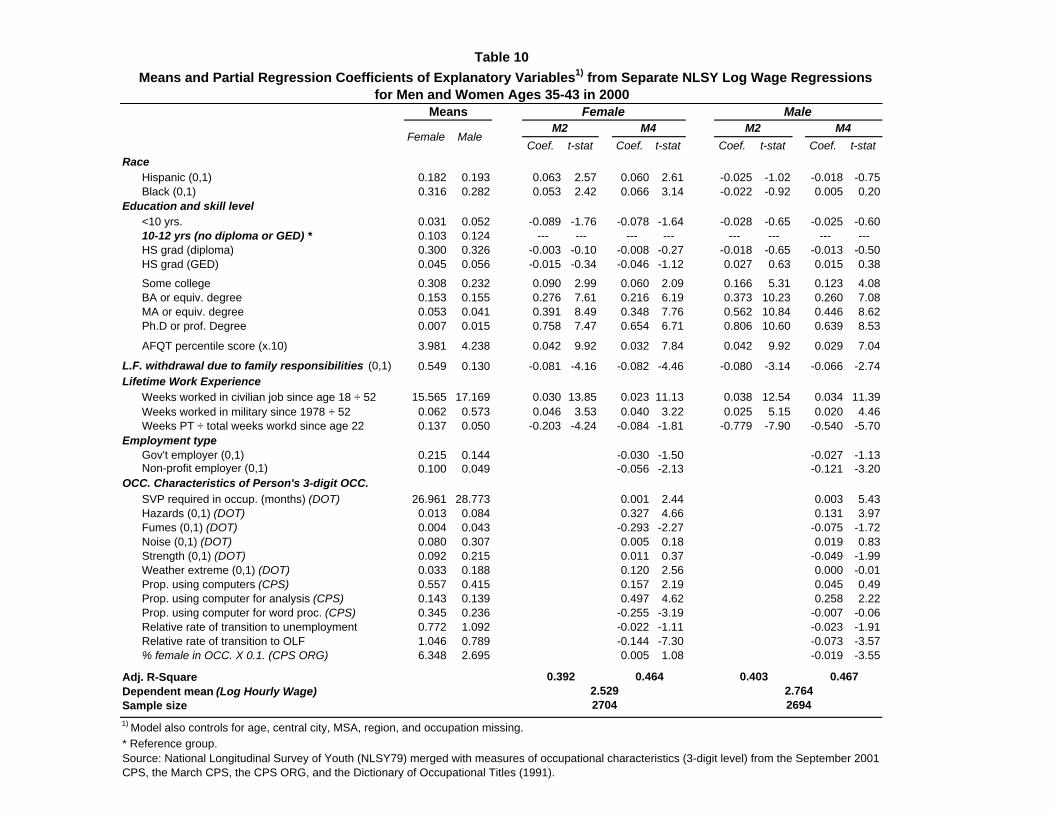
Table 10 Means and Partial Regression Coefficients of Explanatory Variables1) from Separate NLSY Log Wage Regressions

for Men and Women Ages 35-43 in 2000Means Female Male

Female MaleM2 M4 M2 M4

Coef. t-stat Coef. t-stat Coef. t-stat Coef. t-statRace

Hispanic (0,1) 0.182 0.193 0.063 2.57 0.060 2.61 -0.025 -1.02 -0.018 -0.75Black (0,1) 0.316 0.282 0.053 2.42 0.066 3.14 -0.022 -0.92 0.005 0.20

Education and skill level<10 yrs. 0.031 0.052 -0.089 -1.76 -0.078 -1.64 -0.028 -0.65 -0.025 -0.6010-12 yrs (no diploma or GED) * 0.103 0.124 --- --- --- --- --- --- --- ---HS grad (diploma) 0.300 0.326 -0.003 -0.10 -0.008 -0.27 -0.018 -0.65 -0.013 -0.50HS grad (GED) 0.045 0.056 -0.015 -0.34 -0.046 -1.12 0.027 0.63 0.015 0.38

Some college 0.308 0.232 0.090 2.99 0.060 2.09 0.166 5.31 0.123 4.08BA or equiv. degree 0.153 0.155 0.276 7.61 0.216 6.19 0.373 10.23 0.260 7.08MA or equiv. degree 0.053 0.041 0.391 8.49 0.348 7.76 0.562 10.84 0.446 8.62Ph.D or prof. Degree 0.007 0.015 0.758 7.47 0.654 6.71 0.806 10.60 0.639 8.53

AFQT percentile score (x.10) 3.981 4.238 0.042 9.92 0.032 7.84 0.042 9.92 0.029 7.04

L.F. withdrawal due to family responsibilities (0,1) 0.549 0.130 -0.081 -4.16 -0.082 -4.46 -0.080 -3.14 -0.066 -2.74Lifetime Work Experience

Weeks worked in civilian job since age 18 ÷ 52 15.565 17.169 0.030 13.85 0.023 11.13 0.038 12.54 0.034 11.39Weeks worked in military since 1978 ÷ 52 0.062 0.573 0.046 3.53 0.040 3.22 0.025 5.15 0.020 4.46Weeks PT ÷ total weeks workd since age 22 0.137 0.050 -0.203 -4.24 -0.084 -1.81 -0.779 -7.90 -0.540 -5.70

Employment typeGov't employer (0,1) 0.215 0.144 -0.030 -1.50 -0.027 -1.13Non-profit employer (0,1) 0.100 0.049 -0.056 -2.13 -0.121 -3.20

OCC. Characteristics of Person's 3-digit OCC.SVP required in occup. (months) (DOT) 26.961 28.773 0.001 2.44 0.003 5.43Hazards (0,1) (DOT) 0.013 0.084 0.327 4.66 0.131 3.97Fumes (0,1) (DOT) 0.004 0.043 -0.293 -2.27 -0.075 -1.72Noise (0,1) (DOT) 0.080 0.307 0.005 0.18 0.019 0.83Strength (0,1) (DOT) 0.092 0.215 0.011 0.37 -0.049 -1.99Weather extreme (0,1) (DOT) 0.033 0.188 0.120 2.56 0.000 -0.01Prop. using computers (CPS) 0.557 0.415 0.157 2.19 0.045 0.49Prop. using computer for analysis (CPS) 0.143 0.139 0.497 4.62 0.258 2.22Prop. using computer for word proc. (CPS) 0.345 0.236 -0.255 -3.19 -0.007 -0.06Relative rate of transition to unemployment 0.772 1.092 -0.022 -1.11 -0.023 -1.91Relative rate of transition to OLF 1.046 0.789 -0.144 -7.30 -0.073 -3.57% female in OCC. X 0.1. (CPS ORG) 6.348 2.695 0.005 1.08 -0.019 -3.55

Adj. R-Square 0.392 0.464 0.403 0.467Dependent mean (Log Hourly Wage) 2.529 2.764Sample size 2704 26941) Model also controls for age, central city, MSA, region, and occupation missing.* Reference group.Source: National Longitudinal Survey of Youth (NLSY79) merged with measures of occupational characteristics (3-digit level) from the September 2001 CPS, the March CPS, the CPS ORG, and the Dictionary of Occupational Titles (1991).

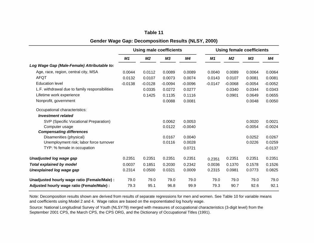
Table 11

Gender Wage Gap: Decomposition Results (NLSY, 2000)

Using male coefficients Using female coefficients

M1 M2 M3 M4 M1 M2 M3 M4

Log Wage Gap (Male-Female) Attributable to:Age, race, region, central city, MSA 0.0044 0.0112 0.0089 0.0089 0.0040 0.0089 0.0064 0.0064AFQT 0.0132 0.0107 0.0073 0.0074 0.0143 0.0107 0.0081 0.0081Education level -0.0138 -0.0128 -0.0094 -0.0096 -0.0147 -0.0068 -0.0054 -0.0052L.F. withdrawal due to family responsibilities 0.0335 0.0272 0.0277 0.0340 0.0344 0.0343Lifetime work experience 0.1425 0.1135 0.1116 0.0901 0.0649 0.0655Nonprofit, government 0.0088 0.0081 0.0048 0.0050

Occupational characteristics: Investment related

SVP (Specific Vocational Preparation) 0.0062 0.0053 0.0020 0.0021Computer usage 0.0122 -0.0040 -0.0054 -0.0024

Compensating differencesDisamenities (physical) 0.0167 0.0040 0.0252 0.0267Unemployment risk; labor force turnover 0.0116 0.0028 0.0226 0.0259

TYP: % female in occupation 0.0721 -0.0137

Unadjusted log wage gap 0.2351 0.2351 0.2351 0.2351 0.2351 0.2351 0.2351 0.2351Total explained by model 0.0037 0.1851 0.2030 0.2342 0.0036 0.1370 0.1578 0.1526Unexplained log wage gap 0.2314 0.0500 0.0321 0.0009 0.2315 0.0981 0.0773 0.0825

Unadjusted hourly wage ratio (Female/Male) : 79.0 79.0 79.0 79.0 79.0 79.0 79.0 79.0Adjusted hourly wage ratio (Female/Male) : 79.3 95.1 96.8 99.9 79.3 90.7 92.6 92.1

Note: Decomposition results shown are derived from results of separate regressions for men and women. See Table 10 for variable means and coefficients using Model 2 and 4. Wage ratios are based on the exponentiated log hourly wage.Source: National Longitudinal Survey of Youth (NLSY79) merged with measures of occupational characteristics (3-digit level) from the September 2001 CPS, the March CPS, the CPS ORG, and the Dictionary of Occupational Titles (1991).

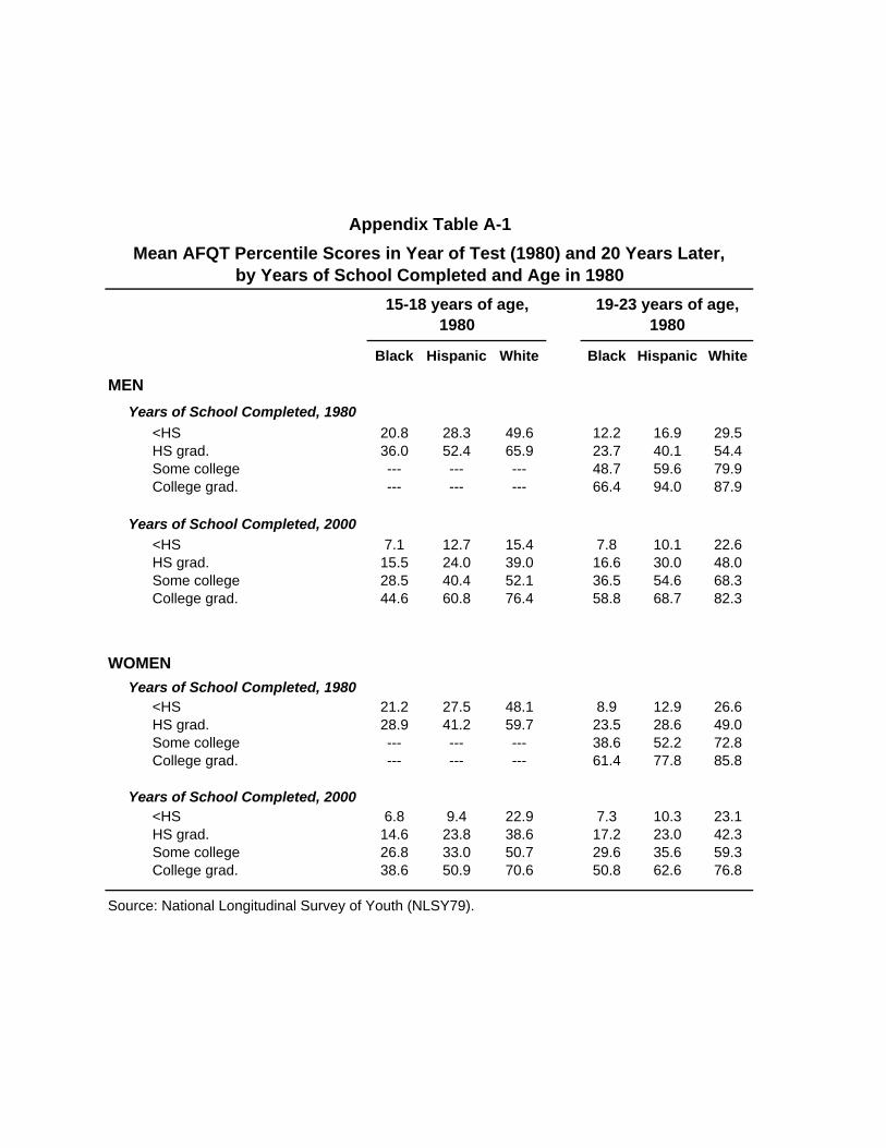
Appendix Table A-1Mean AFQT Percentile Scores in Year of Test (1980) and 20 Years Later,

by Years of School Completed and Age in 198015-18 years of age,

198019-23 years of age,

1980

Black Hispanic White Black Hispanic White

MEN Years of School Completed, 1980

<HS 20.8 28.3 49.6 12.2 16.9 29.5HS grad. 36.0 52.4 65.9 23.7 40.1 54.4Some college --- --- --- 48.7 59.6 79.9College grad. --- --- --- 66.4 94.0 87.9

Years of School Completed, 2000<HS 7.1 12.7 15.4 7.8 10.1 22.6HS grad. 15.5 24.0 39.0 16.6 30.0 48.0Some college 28.5 40.4 52.1 36.5 54.6 68.3College grad. 44.6 60.8 76.4 58.8 68.7 82.3

WOMEN Years of School Completed, 1980

<HS 21.2 27.5 48.1 8.9 12.9 26.6HS grad. 28.9 41.2 59.7 23.5 28.6 49.0Some college --- --- --- 38.6 52.2 72.8College grad. --- --- --- 61.4 77.8 85.8

Years of School Completed, 2000<HS 6.8 9.4 22.9 7.3 10.3 23.1HS grad. 14.6 23.8 38.6 17.2 23.0 42.3Some college 26.8 33.0 50.7 29.6 35.6 59.3College grad. 38.6 50.9 70.6 50.8 62.6 76.8

Source: National Longitudinal Survey of Youth (NLSY79).

,

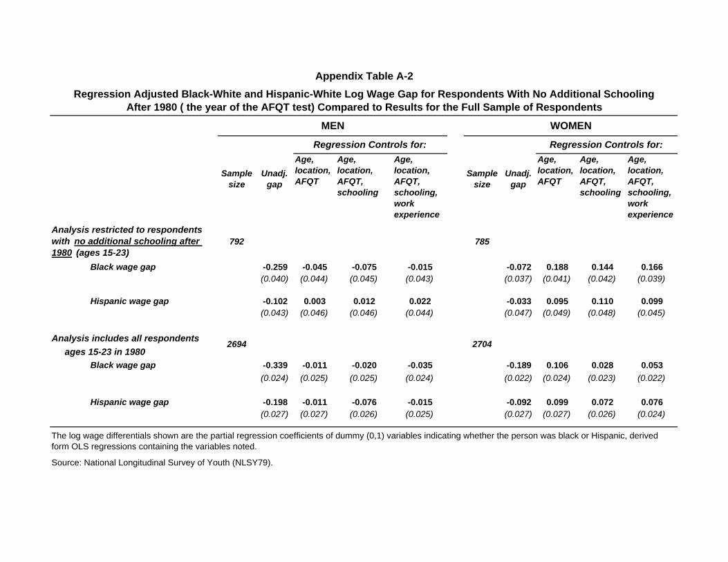
Appendix Table A-2Regression Adjusted Black-White and Hispanic-White Log Wage Gap for Respondents With No Additional Schooling

After 1980 ( the year of the AFQT test) Compared to Results for the Full Sample of Respondents

MEN WOMEN

Sample size

Unadj. gap

Regression Controls for:

Sample size

Unadj. gap

Regression Controls for:Age, location, AFQT

Age, location, AFQT, schooling

Age, location, AFQT, schooling, work experience

Age, location, AFQT

Age, location, AFQT schooling

Age, location, AFQT, schooling, work experience

Analysis restricted to respondents with no additional schooling after 1980 (ages 15-23)

792 785

Black wage gap -0.259 -0.045 -0.075 -0.015 -0.072 0.188 0.144 0.166(0.040) (0.044) (0.045) (0.043) (0.037) (0.041) (0.042) (0.039)

Hispanic wage gap -0.102 0.003 0.012 0.022 -0.033 0.095 0.110 0.099(0.043) (0.046) (0.046) (0.044) (0.047) (0.049) (0.048) (0.045)

Analysis includes all respondents 2694 2704ages 15-23 in 1980

Black wage gap -0.339 -0.011 -0.020 -0.035 -0.189 0.106 0.028 0.053(0.024) (0.025) (0.025) (0.024) (0.022) (0.024) (0.023) (0.022)

Hispanic wage gap -0.198 -0.011 -0.076 -0.015 -0.092 0.099 0.072 0.076(0.027) (0.027) (0.026) (0.025) (0.027) (0.027) (0.026) (0.024)

The log wage differentials shown are the partial regression coefficients of dummy (0,1) variables indicating whether the person was black or Hispanic, derived form OLS regressions containing the variables noted.

Source: National Longitudinal Survey of Youth (NLSY79).

)

)

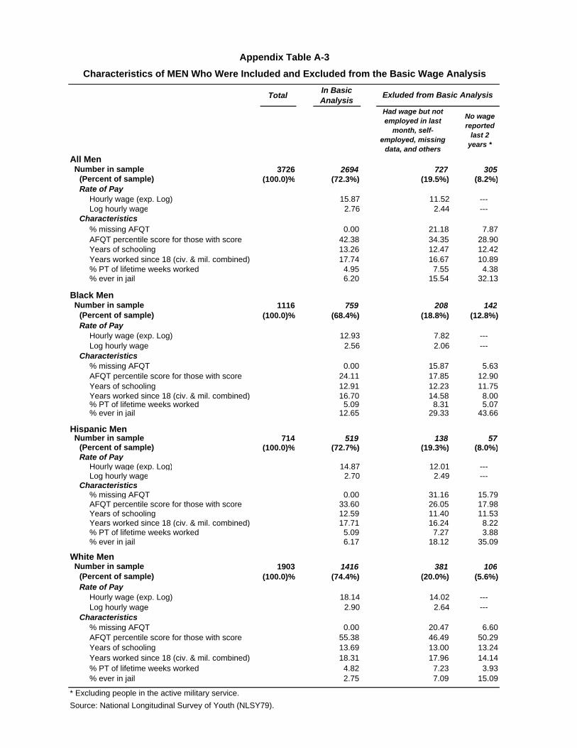
Appendix Table A-3Characteristics of MEN Who Were Included and Excluded from the Basic Wage Analysis

Total In Basic

Analysis Exluded from Basic Analysis

Had wage but not employed in last

month, self-employed, missing

data, and others

No wage reported

last 2 years *

All Men Number in sample 3726 2694 727 305

(Percent of sample) (100.0)% (72.3%) (19.5% (8.2%)Rate of Pay

Hourly wage (exp. Log) 15.87 11.52 ---Log hourly wage 2.76 2.44 ---

Characteristics% missing AFQT 0.00 21.18 7.87AFQT percentile score for those with score 42.38 34.35 28.90Years of schooling 13.26 12.47 12.42Years worked since 18 (civ. & mil. combined) 17.74 16.67 10.89

% PT of lifetime weeks worked 4.95 7.55 4.38% ever in jail 6.20 15.54 32.13

Black Men Number in sample 1116 759 208 142

(Percent of sample) (100.0)% (68.4%) (18.8%) (12.8%)Rate of Pay

Hourly wage (exp. Log) 12.93 7.82 ---Log hourly wage 2.56 2.06 ---

Characteristics% missing AFQT 0.00 15.87 5.63AFQT percentile score for those with score 24.11 17.85 12.90Years of schooling 12.91 12.23 11.75Years worked since 18 (civ. & mil. combined) 16.70 14.58 8.00

% PT of lifetime weeks worked 5.09 8.31 5.07 % ever in jail 12.65 29.33 43.66

Hispanic Men Number in sample 714 519 138 57

(Percent of sample) (100.0)% (72.7%) (19.3% (8.0%)Rate of Pay

Hourly wage (exp. Log) 14.87 12.01 ---Log hourly wage 2.70 2.49 ---

Characteristics% missing AFQT 0.00 31.16 15.79AFQT percentile score for those with score 33.60 26.05 17.98Years of schooling 12.59 11.40 11.53Years worked since 18 (civ. & mil. combined) 17.71 16.24 8.22

% PT of lifetime weeks worked 5.09 7.27 3.88 % ever in jail 6.17 18.12 35.09

White Men Number in sample 1903 1416 381 106

(Percent of sample) (100.0)% (74.4%) (20.0%) (5.6%)Rate of Pay

Hourly wage (exp. Log) 18.14 14.02 ---Log hourly wage 2.90 2.64 ---

Characteristics% missing AFQT 0.00 20.47 6.60AFQT percentile score for those with score 55.38 46.49 50.29Years of schooling 13.69 13.00 13.24Years worked since 18 (civ. & mil. combined) 18.31 17.96 14.14

% PT of lifetime weeks worked 4.82 7.23 3.93 % ever in jail 2.75 7.09 15.09

* Excluding people in the active military service.Source: National Longitudinal Survey of Youth (NLSY79).

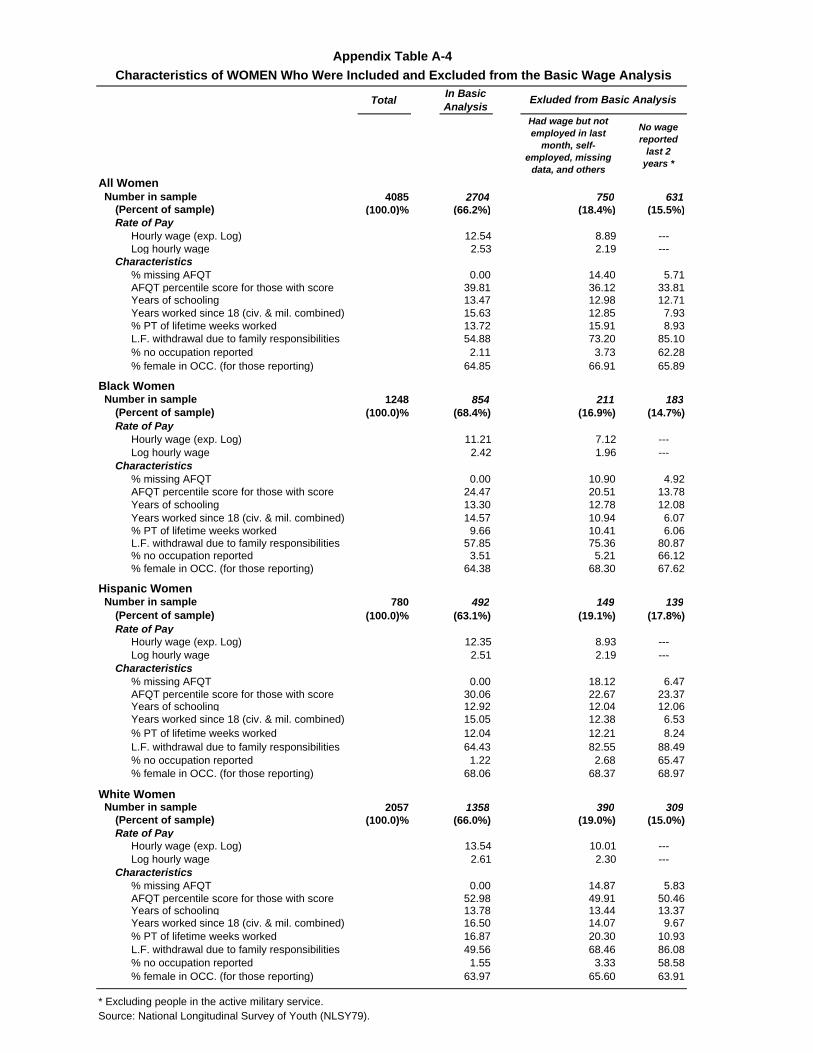
Appendix Table A-4Characteristics of WOMEN Who Were Included and Excluded from the Basic Wage Analysis

Total In Basic

Analysis Exluded from Basic Analysis

Had wage but not employed in last

month, self-employed, missing

data, and others

No wage reported

last 2 years *

All Women Number in sample 4085 2704 750 631

(Percent of sample) (100.0)% (66.2%) (18.4%) (15.5%)Rate of Pay

Hourly wage (exp. Log) 12.54 8.89 ---Log hourly wage 2.53 2.19 ---

Characteristics% missing AFQT 0.00 14.40 5.71AFQT percentile score for those with score 39.81 36.12 33.81Years of schooling 13.47 12.98 12.71Years worked since 18 (civ. & mil. combined) 15.63 12.85 7.93

% PT of lifetime weeks worked 13.72 15.91 8.93 L.F. withdrawal due to family responsibilities 54.88 73.20 85.10

% no occupation reported 2.11 3.73 62.28% female in OCC. (for those reporting) 64.85 66.91 65.89

Black Women Number in sample 1248 854 211 183

(Percent of sample) (100.0)% (68.4%) (16.9%) (14.7%)Rate of Pay

Hourly wage (exp. Log) 11.21 7.12 ---Log hourly wage 2.42 1.96 ---

Characteristics% missing AFQT 0.00 10.90 4.92AFQT percentile score for those with score 24.47 20.51 13.78Years of schooling 13.30 12.78 12.08Years worked since 18 (civ. & mil. combined) 14.57 10.94 6.07

% PT of lifetime weeks worked 9.66 10.41 6.06 L.F. withdrawal due to family responsibilities 57.85 75.36 80.87

% no occupation reported 3.51 5.21 66.12% female in OCC. (for those reporting) 64.38 68.30 67.62

Hispanic Women Number in sample 780 492 149 139

(Percent of sample) (100.0)% (63.1%) (19.1%) (17.8%)Rate of Pay

Hourly wage (exp. Log) 12.35 8.93 ---Log hourly wage 2.51 2.19 ---

Characteristics% missing AFQT 0.00 18.12 6.47AFQT percentile score for those with score 30.06 22.67 23.37Years of schooling 12.92 12.04 12.06Years worked since 18 (civ. & mil. combined) 15.05 12.38 6.53

% PT of lifetime weeks worked 12.04 12.21 8.24 L.F. withdrawal due to family responsibilities 64.43 82.55 88.49

% no occupation reported 1.22 2.68 65.47% female in OCC. (for those reporting) 68.06 68.37 68.97

White Women Number in sample 2057 1358 390 309

(Percent of sample) (100.0)% (66.0%) (19.0%) (15.0%)Rate of Pay

Hourly wage (exp. Log) 13.54 10.01 ---Log hourly wage 2.61 2.30 ---

Characteristics% missing AFQT 0.00 14.87 5.83AFQT percentile score for those with score 52.98 49.91 50.46Years of schooling 13.78 13.44 13.37Years worked since 18 (civ. & mil. combined) 16.50 14.07 9.67

% PT of lifetime weeks worked 16.87 20.30 10.93 L.F. withdrawal due to family responsibilities 49.56 68.46 86.08

% no occupation reported 1.55 3.33 58.58% female in OCC. (for those reporting) 63.97 65.60 63.91

* Excluding people in the active military service.Source: National Longitudinal Survey of Youth (NLSY79).

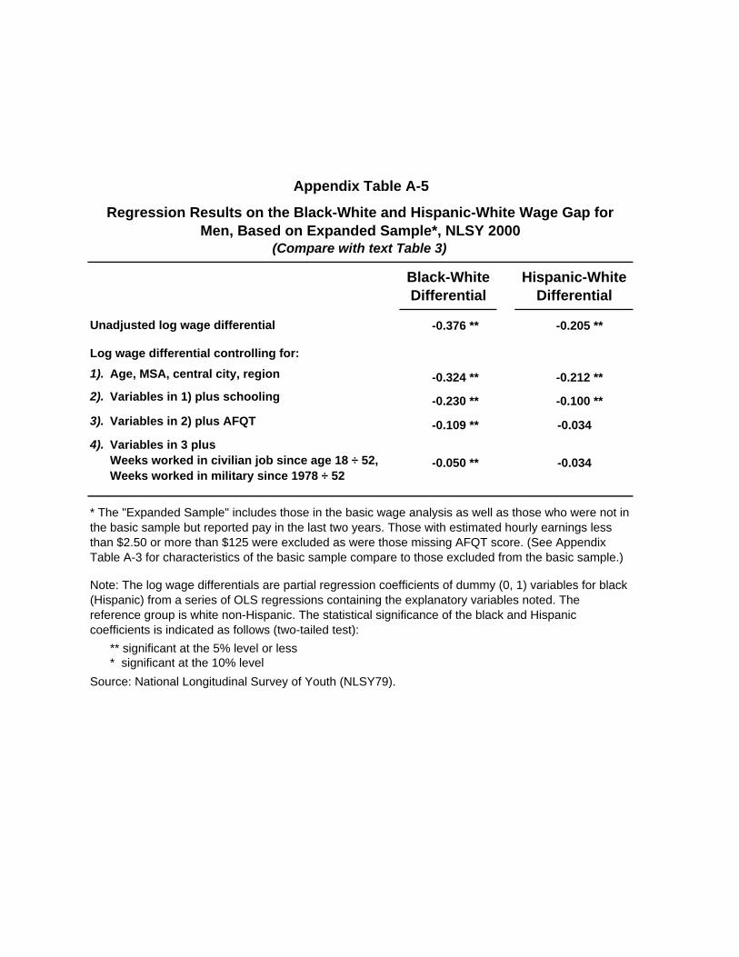
Appendix Table A-5

Regression Results on the Black-White and Hispanic-White Wage Gap for Men, Based on Expanded Sample*, NLSY 2000

(Compare with text Table 3)

Black-White Differential

Hispanic-White Differential

Unadjusted log wage differential -0.376 ** -0.205 **

Log wage differential controlling for:1). Age, MSA, central city, region -0.324 ** -0.212 **2). Variables in 1) plus schooling -0.230 ** -0.100 **3). Variables in 2) plus AFQT -0.109 ** -0.0344). Variables in 3 plus

Weeks worked in civilian job since age 18 ÷ 52, Weeks worked in military since 1978 ÷ 52

-0.050 ** -0.034

* The "Expanded Sample" includes those in the basic wage analysis as well as those who were not in the basic sample but reported pay in the last two years. Those with estimated hourly earnings less than $2.50 or more than $125 were excluded as were those missing AFQT score. (See Appendix Table A-3 for characteristics of the basic sample compare to those excluded from the basic sample.)

Note: The log wage differentials are partial regression coefficients of dummy (0, 1) variables for black (Hispanic) from a series of OLS regressions containing the explanatory variables noted. The reference group is white non-Hispanic. The statistical significance of the black and Hispanic coefficients is indicated as follows (two-tailed test):

** significant at the 5% level or less* significant at the 10% level

Source: National Longitudinal Survey of Youth (NLSY79).

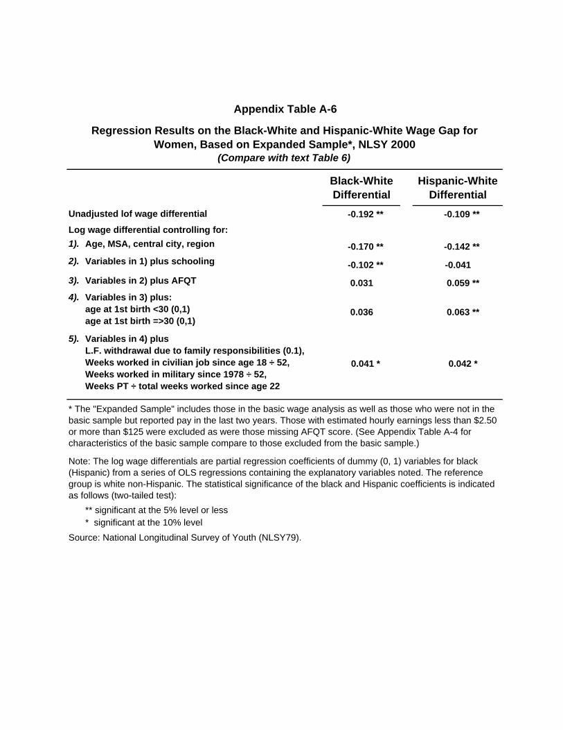
Appendix Table A-6

Regression Results on the Black-White and Hispanic-White Wage Gap for Women, Based on Expanded Sample*, NLSY 2000

(Compare with text Table 6)

Black-White Differential

Hispanic-White Differential

Unadjusted lof wage differential -0.192 ** -0.109 **Log wage differential controlling for:1). Age, MSA, central city, region -0.170 ** -0.142 **2). Variables in 1) plus schooling -0.102 ** -0.0413). Variables in 2) plus AFQT 0.031 0.059 **4). Variables in 3) plus:

age at 1st birth <30 (0,1) age at 1st birth =>30 (0,1)

0.036 0.063 **

5). Variables in 4) plus L.F. withdrawal due to family responsibilities (0.1), Weeks worked in civilian job since age 18 ÷ 52, Weeks worked in military since 1978 ÷ 52, Weeks PT ÷ total weeks worked since age 22

0.041 * 0.042 *

* The "Expanded Sample" includes those in the basic wage analysis as well as those who were not in the basic sample but reported pay in the last two years. Those with estimated hourly earnings less than $2.50 or more than $125 were excluded as were those missing AFQT score. (See Appendix Table A-4 for characteristics of the basic sample compare to those excluded from the basic sample.)

Note: The log wage differentials are partial regression coefficients of dummy (0, 1) variables for black (Hispanic) from a series of OLS regressions containing the explanatory variables noted. The reference group is white non-Hispanic. The statistical significance of the black and Hispanic coefficients is indicated as follows (two-tailed test):

** significant at the 5% level or less* significant at the 10% level

Source: National Longitudinal Survey of Youth (NLSY79).

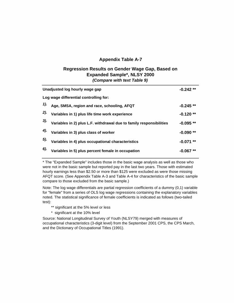
Appendix Table A-7

Regression Results on Gender Wage Gap, Based on Expanded Sample*, NLSY 2000

(Compare with text Table 9)

Unadjusted log hourly wage gap -0.242 **

Log wage differential controlling for:

1). Age, SMSA, region and race, schooling, AFQT -0.245 **2). Variables in 1) plus life time work experience -0.120 ** 3). Variables in 2) plus L.F. withdrawal due to family responsibilities -0.095 **4). Variables in 3) plus class of worker -0.090 **5). Variables in 4) plus occupational characteristics -0.071 **6). Variables in 5) plus percent female in occupation -0.067 **

* The "Expanded Sample" includes those in the basic wage analysis as well as those who were not in the basic sample but reported pay in the last two years. Those with estimated hourly earnings less than $2.50 or more than $125 were excluded as were those missing AFQT score. (See Appendix Table A-3 and Table A-4 for characteristics of the basic sample compare to those excluded from the basic sample.)

Note: The log wage differentials are partial regression coefficients of a dummy (0,1) variable for "female" from a series of OLS log wage regressions containing the explanatory variables noted. The statistical significance of female coefficients is indicated as follows (two-tailed test):

** significant at the 5% level or less* significant at the 10% level

Source: National Longitudinal Survey of Youth (NLSY79) merged with measures of occupational characteristics (3-digit level) from the September 2001 CPS, the CPS March, and the Dictionary of Occupational Titles (1991).