NBER WORKING PAPER SERIES

WOMEN, WAR AND WAGES:

THE EFFECT OF FEMALE LABOR SUPPLY ON

THE WAGE STRUCTURE AT MID-CENTURY

Daron Acemoglu

David H. Autor

David Lyle

Working Paper 9013

http://www.nber.org/papers/w9013

NATIONAL BUREAU OF ECONOMIC RESEARCH

1050 Massachusetts Avenue

Cambridge, MA 02138

June 2002

We thank Joshua Angrist, John Bound, David Card, Olivier Deschênes, Alan Krueger, Lawrence Katz, Peter

Kuhn, Casey Mulligan, Bas ter Weel, Linda Wong, and seminar participants at UC Berkeley, Università

Bocconi, the European University Institute, the University of Michigan, MIT, UC Santa Barbara, UC Santa

Cruz, Stanford University, UCLA, University of British Columbia and Wharton for valuable suggestions,

and the National Science Foundation and the Russell Sage Foundation for financial support. The views

expressed herein are those of the authors and not necessarily those of the National Bureau of Economic

Research.

© 2002 by Daron Acemoglu, David H. Autor and David Lyle. All rights reserved. Short sections of text,

not to exceed two paragraphs, may be quoted without explicit permission provided that full credit, including

© notice, is given to the source.

Women, War and Wages: The Effect of Female Labor Supply

on the Wage Structure at Mid-Century

Daron Acemoglu, David H. Autor and David Lyle

NBER Working Paper No. 9013

June 2002

JEL No. J21, J22, J31, J16, N32, H56

ABSTRACT

This paper investigates the effects of female labor supply on the wage structure. To identify

variation in female labor supply, we exploit the military mobilization for World War II, which drew many

women into the workforce as males exited civilian employment. The extent of mobilization was not

uniform across states, however, with the fraction of eligible males serving ranging from 41 to 54 percent.

We find that in states with greater mobilization of men, women worked substantially more after the War

and in 1950, though not in 1940. We interpret these differentials as labor supply shifts induced by the

War. We find that increases in female labor supply lower female wages, lower male wages, and increase

the college premium and male wage inequality generally. Our findings indicate that at mid-century,

women were closer substitutes to high school graduate and relatively low-skill males, but not to those

with the lowest skills.

Daron Acemoglu David H. Autor David Lyle

Department of Economics Department of Economics Department of Economics

MIT, E52-380B MIT, E52-371 MIT

50 Memorial Drive 50 Memorial Drive 50 Memorial Drive

Cambridge, MA 02142-1347 Cambridge, MA 02142-1347 Cambridge, MA 02142-1347

and NBER and NBER dlyle@mit.edu

daron@mit.edu dautor@mit.edu

“In May, 1947, 31.5 per cent of all women 14 years of age and over were workers as

compared to 27.6 per cent in 1940. This proportion has been increasing for many

decades. However, both the number and the proportion of women working in 1947

are believed to be greater than would have been expected in this year had there not

been a war.” Constance Williams, Chief of the Research Division of the Women’s

Bureau of the United States Department of Labor, 1949.

1 Introduction

In 1900, 82 percent of U.S. workers were male, and only 18 percent of women over the age of

15 participated in the labor force. As is visible in Figure 1, this picture changed radically over

the course of the past century. In 2001, 47 percent of U.S. workers were women, and 61 percent

of women over the age of 15 were in the labor force. Despite these epochal changes in women’s

labor force participation, economists currently know relatively little about how female labor

force participation affects the labor market.

• Does it increase or decrease male wages?

• Does it adversely affect female wages?

• Does it impact male wage inequality?

The relative scarcity of convincing studies on this topic reflects the complexity of the phe-

nomenon: increased labor participation of women is driven both by supply and demand factors.

Women participate in the labor force more today than 100 years ago for a myriad of supply-

side reasons including changes in tastes, gender roles and technology of household production.

But women also participate more because there is greater demand for their labor services. To

advance our understanding of how rising female labor force participation impacts the labor

market, we require a source of “exogenous” variation in female labor supply.

In this paper, we study female labor force participation before and after World War II

(WWII) as a source of plausibly exogenous variation in female labor supply. As evocatively

captured by the image of Rosie the Riveter, the War drew many women into the labor force as

16 million men mobilized to serve in the armed forces, with over 73 percent leaving for overseas.

As is depicted in Figure 2, only 28 percent of U.S. women over the age of 15 participated in

1

the labor force in 1940. By 1945 this figure exceeded 34 percent.1 Although, as documented by

Goldin (1991), more than half of the women drawn into the labor force by the War left again

by the end of the decade, a substantial number also remained (see also Clark and Summers,

1982). In fact, the decade of the 1940s saw the largest proportional rise in female labor force

participation during the 20th century.

Although this aggregate increase in female labor force participation is evident from Figures

1 and 2, it is not particularly useful for our purposes; the end of the War and other aggregate

factors make the early 1950s difficult to compare to other decades. But, central to our research

strategy, the extent of mobilization for the War was not uniform across U.S. states. While

in some states, for example Massachusetts, Oregon, and Utah, almost 55 percent of males

between the ages of 18 and 44 left the labor market to serve in the War, in other states, such

as Georgia, the Dakotas and the Carolinas, this number was between 40 and 45 percent. These

differences in mobilization rates reflect a variety of factors, including exemptions for farmers,

differences in age, ethnic and occupational structures, as well as idiosyncratic differences in the

behavior of local draft boards. We exploit differences in state WWII mobilization rates, as

well as components of these mobilization rate differences that are plausibly exogenous to other

labor market outcomes, to study women’s labor supply.

Panels A and B of Figure 3 show that women worked substantially more in 1950–but not

in 1940–in states with greater mobilization of men during the War (see below for the exact

definition of the mobilization variable). Our baseline estimates suggest that women worked

on average about 1 week more in a state that had a 10 percentage point higher mobilization

rate during WWII, corresponding to a 9 percentage point increase in female labor supply. This

difference is not accounted for by differences in age structure, racial structure, education or

the importance of farming across these states, nor is it explained by differences in occupational

structure, regional trends in labor supply, or contrasts between Southern and non-Southern

states. We interpret these cross-state changes in female employment as caused by the greater

participation of women during the War years, some of whom stayed in the labor market after

the War ended. Notably, we find in Panel C of Figure 3 that the sizable association between

WWII mobilization rates and growth in female labor supply over the 1940s did not recur in

the 1950s, lending support to the hypothesis that these shifts were caused by the War, and not1For convenience, we refer to Census years as 1940, 1950, etc. In reality, Census data provides labor supply

information for the prior calendar year.

2

by differential long-run trends in female employment.

Panel A of Figure 4 shows an equally strong relationship between female wage growth over

the 1940s and WWII mobilization rates: in states with greater mobilization for war, female

wages grew much less. Panel B shows a negative relationship for male wages as well, but the

slope of the relationship is considerably less steep.

We interpret the relationships shown in Figure 4 as the causal effect of the WWII-induced

increase in female labor supply on female and male wages. As Figure 2 shows, the aggregate

demand shock that drew many women into the labor force during the mobilization years had

reversed itself by 1947. But women continued to work in greater numbers after 1947, presumably

because employment during the War changed their preferences, opportunities and information

about available work.

Our interpretation of the relationship between mobilization, female labor supply, and wage

growth faces two major challenges:

1. High- and low-mobilization states may be different in other unobserved dimensions. In

that case, Figure 3 and 4 may be capturing the effect of these unobserved characteristics

on labor market outcomes, and our identification strategy may be assigning the effects of

these unobserved state characteristics on labor market outcomes to female labor supply.

2. Mobilization of men for war may have had a direct effect on the labor market, distinct from

its impact through female labor supply. For example, men who served in the War may

have had difficulty reintegrating into the workforce, or may have entered school instead

due to the opportunities offered by the GI Bills (Bound and Turner, 1999; Stanley, 1999).

If this were the case, our first-stage finding of a relationship between mobilization and

female labor supply would remain valid, but our two-stage least square (2SLS) estimates

would be biased: greater female labor force participation in high-mobilization states could

reflect greater demand for female labor input rather than shifts in female labor supply.

Although we cannot dismiss these two interpretations entirely, we provide evidence to sug-

gest that they are not the primary source of our findings. Our results are typically robust to

including a variety of aggregate characteristics of states, including fraction of farmers before

the War, racial, education, and occupational structures. We also obtain similar results when we

focus on the component of mobilization rate generated by cross-state differences in aggregate

3

age and ethnic structure, which were important determinants of state mobilization rates, but

should plausibly have no direct effect on female labor supply growth once we condition on indi-

vidual age and ethnicity. These findings weigh against an interpretation along the lines of the

first objection above. Moreover, female labor force participation did not vary systematically

between high- and low-mobilization states prior to the War, suggesting that these states were

initially broadly comparable along this dimension. Finally, as Panel C of Figure 3 documents,

high-mobilization states did not experience faster growth in female employment between 1950

and 1960. Hence, there do not appear to be differential state employment trends correlated

with WWII mobilization rates.

If, on the other hand, the second concern were important–that is, if returning veterans

had trouble reintegrating into the labor market–there should be lower labor force participa-

tion among men in 1950 in high-mobilization states. We find that this is generally not the

case. Men who were not mobilized appear to participate slightly more after the War in high-

mobilization states. And post-war labor supply of WWII veterans in 1950 is, for the most part,

comparable across high and low-mobilization states, though some specifications do show nega-

tive but insignificant effects. Furthermore, if greater female participation in 1950 were driven

by demand rather than supply factors, we would expect relatively greater wage growth for both

women and men in high-mobilization states. Instead, consistent with our interpretation, Figure

4 shows that both men and women earned relatively less in high-mobilization states in 1950

than in 1940. Nor are our results driven by cross-state wage convergence between agricultural

and industrialized states during the 1940s (e.g., Wright, 1986); in specifications that control

for lagged state wage measures, we continue to find a significant impact of mobilization on the

structure of male and female earnings. Finally, Figure 5 shows no relationship between state

WWII mobilization rates and wage growth between 1950 and 1960. Hence, the cross-state

correlations that we exploit between WWII mobilization and female labor supply or relative

wage changes by gender appear unique to the WWII decade.

Exploiting the differential growth in female employment between 1940 and 1950 related to

cross-state differences in WWII mobilization, we estimate the impact of female employment on

a range of labor market outcomes. Our main findings are:

1. Greater female labor supply reduces female wages. A ten percent increase in relative

female labor supply (that is, relative to males) lowers female wages by 6 to 7 percent,

4

implying a labor demand elasticity of -1.4 to -1.7.

2. Greater female labor supply also reduces male wages. A 10 percent increase in the (log)

ratio of female to male labor supply typically lowers male earnings by 3 to 5 percent.

3. The finding that female labor supply lowers women’s wages by more than men’s indicates

that male and female labor inputs are imperfect substitutes. We estimate that a 10 percent

increase in relative supply reduces relative female/male earnings by about 3 percentage

points. This implies a substitution elasticity of approximately 3, which is large but far

from perfect substitutability.

4. The impact of female labor supply on male earnings is not uniform throughout the male

earnings distribution. A 10 percent increase in female relative labor supply raises earnings

inequality between college and high school graduate males by about 1.5 percentage points

and lowers earnings inequality between high school graduate and eight-grade males by

about 2 percentage points. These findings indicate that the women drawn into the labor

market by the War were closer substitutes to males at the middle of the skill distribution

than those with either the lowest or highest education.

5. Although female labor supply has countervailing effects on educational differentials, its

net impact on overall and residual earnings inequality among males is positive. A 10

percent increase in female labor supply is estimated to increase the male 90-10 weekly

earnings differential by 5.5 log points, which is a very sizable effect.

It is important to note that these estimates conceptually correspond to short-run elasticities

since we are looking at equilibria in state labor markets shortly after the War, that is, shortly

after the changes in female labor supply. Migration, changes in interstate trade patterns and

changes in technologies could make the long-run relationship between labor market outcomes

and female labor supply quite different from the short-run relationship. Results exploiting

changes between 1940 and 1960 suggest that long-run elasticities are indeed larger than short-

run elasticities.

The economics literatures on the effect of WWII on female participation and the effect of

female labor supply on the structure of wages contains a small number of well-known contribu-

tions. Goldin (1991) is most closely related to our work. She investigates the effects of WWII

5

on women’s labor force participation and finds that a little over half of the women who entered

the labor market during the War years exited by 1950. Our labor supply estimates appear

consistent with these findings, though differences in the sample frame make it difficult to make

exact comparisons. Mulligan (1998) investigates the causes of the increase in labor supply

during the War, and concludes that non-pecuniary factors rather than market incentives drove

this growth. Neither Goldin nor Mulligan nor, to the best of our knowledge, any other author

investigates the relationship between cross-state mobilization rates and female labor supply,

nor the causal effect of the induced change in female labor supply on labor market outcomes of

men.2

Blau and Kahn (1999), Juhn and Kim (1999), Topel (1994 and 1997) and the short papers

by Fortin and Lemieux (2000) andWelch (2000) also investigate the effect of female employment

growth on male wage inequality.3 Using Current Population Survey data from 1968-1990, Topel

(1994) finds a strong positive correlation between regional changes in female labor supply and

growth in male earnings inequality. By contrast, Juhn and Kim (1999) do not find a sizable

effect of female labor supply on male wage inequality in a cross-state Census panel. Fortin

and Lemieux hypothesize that the increase in male wage inequality during the past several

decades may reflect the process of women substituting for males in the earnings distribution,

and provide time-series evidence on the correlations between percentiles of the male and female

wage distribution that are consistent with this hypothesis. Finally, Welch (2000) links both

the decline in the wages of low-skill men and the narrowing of the male-female wage gap over

the past three decades to the overall increase in the demand for skills. While each of these

analyses reaches provocative, albeit divergent, conclusions, the identification strategies used do

not provide a means to separate supply- and demand-induced changes in female employment.

What distinguishes our analysis is the use of plausibly exogenous variation in female labor

market participation induced by World War II mobilization.

In the next section, we briefly discuss the predictions of a simple competitive model regarding

the effect of increased female labor force participation on male labor market outcomes. Section2An unpublished dissertation by Dresser (1994) studies the relationship between federal war contracts and

labor market participation of women across metropolitan areas and finds that MSAs that had a relatively largenumber of war contracts during the war experienced differential increases in female labor force participationbetween 1940 and 1950.

3Goldin and Margo (1992) provide the seminal work on changes in the overall structure of earnings duringthe decade of the War. For excellent syntheses of the state of knowledge of the role of women in the laborforce, see Goldin (1990 and 1994), Blau, Ferber and Winkler (2002), Blau and Kahn (1994, 1997 and 2000),and O’Neill and Polachek (1993).

6

3 describes our microdata and documents the correlation between female employment and a

range of female and male labor market outcomes. In Section 4, we provide a brief overview of

the draft and enlistment process for World War II, and explain the causes of the substantial

differences in mobilization rates across states. Section 5 documents the relationship between

WWII mobilization rates and female labor supply in 1950, and argues that mobilization rates

generate a plausible source of exogenous variation in female labor supply. Sections 6 and 7

contain our main results. They exploit cross-state differences in female labor supply induced

by mobilization rates to estimate the impact of increased female labor supply on female wages

and male wages, educational inequality, and overall earnings inequality among males. Section

8 concludes.

2 Some Simple Theoretical Ideas

To frame the key questions of this investigation, it is useful to briefly discuss the theoreti-

cal implications of increased female labor force participation. Consider a competitive labor

market consisting of four factors: high-skill males, Ht, low-skill males, Lt, females, Ft, and

capital, Kt, which stands for all nonlabor inputs.4 Imagine that all these factors are imper-

fectly substitutable in the production of a single final good. In particular, to fix ideas, consider

the following nested CES (constant elasticity of substitution) aggregate production function,

where, to simplify notation, we ignore the share parameters:

Yt = AtK1−αt

h¡BLt Lt

¢η+¡¡BFt Ft

¢ρ+¡BHt Ht

¢ρ¢η/ρiα/η,

where At is a neutral productivity term, and the Bt’s are factor-augmenting productivity terms,

which are for now taken as exogenous. In particular, BFt is an index of female productivity,

which may reflect observed or unobserved components of female human capital as well as

technical change favoring women relative to men. This specification assumes that the elasticity

of substitution between the labor aggregate and nonlabor inputs is equal to 1, the elasticity

of substitution between female labor and high-skill male labor is 1/ (1− ρ), and the elasticity

of substitution between low-skill male labor and the aggregate between female and high-skill

male labor is 1/ (1− η). When η > ρ, female labor competes more with low-skill male labor4We do not distinguish between high- and low-skill females both to reduce the number of factors and because,

in the empirical work, we will only have a source of exogneous variation in the total number (or total efficiencyunits) of females in the labor force.

7

than high-skill male labor, whereas when η < ρ, it competes more with high-skill male labor.

This nested CES is similar to the one used by Krusell et al. (2000) with high-skill and low-skill

labor, and equipment capital.

In this model, the wage ratio of high-skill to low-skill male wages, corresponding to the skill

or education premium, is a natural index of male wage inequality. Since in competitive labor

markets, wages are equal to marginal products, this ratio will be

ωt ≡ wht

wllt=BHtBLt

¡BHt Ht

¢ρ−1 ¡¡BFt Ft

¢ρ+¡BHt Ht

¢ρ¢(η−ρ)/ρ(BLt Lt)

η−1

It is then straightforward to show that

Sign¿

∂ωt∂BFt Ft

À= Sign hη − ρi ,

that is, an increase in effective female labor supply increases male wage inequality when women

compete more with low-skill males than with high-skill males, i.e., when η > ρ. If female

labor has traditionally been a closer substitute to low-skill male labor than high-skill male

labor as argued by Grant and Hamermesh (1981) and Topel (1994 and 1997) among others, we

may expect increased female labor force participation to act as a force towards greater wage

inequality among men. The empirical magnitude of this effect is unclear, however.

The effect of increased female labor force participation on average wages of men, or on the

level of high-skill and low-skill wages, depends upon the elasticity of supply of nonlabor inputs.

It is straightforward to verify that if these nonlabor inputs are supplied elastically (or if α = 1),

increased female labor supply will always raise average male wages. If, on the other hand,

the supply of nonlabor inputs to the economy is upward sloping, the effect is ambiguous, and

depends on the elasticity of substitution between male and female labor and on the response

of the rental price of these nonlabor inputs to the increase in female labor supply.

More explicitly, low-skill male wages are

wlt = αAtK1−αt

h¡BLt Lt

¢η+¡¡BFt Ft

¢ρ+¡BHt Ht

¢ρ¢η/ρi(α−η)/η ¡BLt Lt

¢η−1.

Holding the supply of nonlabor inputs fixed, we have that

Sign¿

∂wlt∂BFt Ft

À= Sign hα− ηi . (1)

8

In other words, when the elasticity of substitution parameter, η, is sufficiently high relative

to the share of labor in production, α, an increase in female labor supply will reduce the

(conditional) demand for and the earnings of low-skill males. In what follows, we will loosely

refer to female and (a particular type of) male labor as “close substitutes” when greater female

employment reduces the wages of that type of male labor, since a greater level of η (i.e., a

greater elasticity of substitution) makes such negative wage effects more likely.

The same trade-offs determine whether average male wages increase or decline in response

to increased female labor force participation. Substitution of female labor for male labor, by

reducing the ratio of nonlabor inputs to effective labor, acts to depress earnings, while the

complementarity between female and male labor raises the earnings of men. The overall effect

will be determined by which of these two forces is stronger.

Can we use this framework to interpret the relationship between female labor supply and

wages at the state level in the aftermath of WWII? There are at least three caveats that apply:

1. This interpretation requires U.S. states to approximate separate labor markets. This

may be problematic if either migration makes the entire U.S. a single labor market,

or if local labor markets are at the city or MSA level. Both problems would cause

attenuation, which does not bias instrumental-variables estimates, but makes them less

precise. For example, in the extreme case where migration is free and rapid, there would be

no systematic relative employment and factor price differences across state labor markets.

Many studies, however, find migration to be less than perfect in the short run (e.g.,

Blanchard and Katz, 1992, Bound and Holzer, 2000, Card and DiNardo, 2000), while

others document significant wage differences across state or city labor markets (e.g., Topel,

1994, Acemoglu and Angrist, 2000, Moretti, 2000, Bernard, Jensen and Schott, 2001,

Hanson and Slaughter, 2002, forthcoming).Our results also show substantial differences

in relative employment and wages across states related to WWII mobilization.

2. The single-good setup is an important simplification. When there are multiple goods

with different factor proportions, trade between different labor markets can also serve

to equalize factor prices (Samuelson, 1948). It is reasonable to presume that changes in

interstate trade patterns required to achieve factor price equalization do not take place

9

in the short run.5

3. Short-run and long-run elasticities may also vary significantly, either because there are

factors, such as capital or entrepreneurial skills, that adjust only slowly (cf, the LeChater-

lier principle in Samuelson, 1947), or because technology (organization of production) is

endogenous and responds to the availability of factors (Acemoglu, 1998, 2002).

In light of all these caveats, the elasticities we estimate in this paper should be interpreted as

short-run elasticities (except when we look at the two-decade change between 1940 and 1960).

The majority of the estimates exploit the differential increase in female labor supply at the end

of the War on labor market outcomes shortly after the War. Migration, changes in interstate

trade patterns and changes in technologies are likely to make the long-run relationship between

female labor supply and labor market outcomes quite different from the short-run relationship.

3 Data Sources and OLS Estimates

3.1 Data

Our basic data come from the one-percent Integrated Public Use Microsamples (IPUMS) of the

decennial Censuses. Samples include males and females ages 14-64 in the year for which earnings

are reported who are not residing in institutional groups quarters (such as prisons or barracks),

are not employed in farming, and who reside in the continental United States. Throughout the

paper, we exclude Alaska, Hawaii, Washington D.C. and Nevada from the analysis. Alaska and

Hawaii were not states until the 1950s, while Nevada underwent substantial population changes

during the critical period of our analysis.6 The 1950 sample is further limited to the sample-line

subsample because educational attainment is not reported in the full sample. Sampling weights

are employed in all calculations. Earnings samples include all full-time, full-year workers in paid

non-farm employment excluding self-employed who earned the equivalent of $0.50 to $250 an

hour in 1990 dollars during the previous year (deflated by CPI All Urban Consumers series

CUUR0000SA0). Weekly earnings are computed as total wage and salary income earned in the

previous year divided by weeks worked in the previous year, and hourly earnings are computed

as wage/salary income divided by weeks worked in the previous year and hours worked in the5This is especially true at midcentury, since construction of the U.S. Interstate Highway System did not

begin until 1956 with the authorization of the Federal Aid-Highway Act.6Nevada had an extremely high mobilization rate, yet despite this, lies directly along the regression line for

most of our analyses. Inclusion of Nevada affects none of our results

10

previous week.7 Top coded earnings values are imputed as 1.5 times the censored value. We

define full-time, full-year employment as working at least 35 hours in the survey week and 40

weeks in the previous year. Because weeks worked in 1940 are reported as full-time equivalent

weeks, we do not impose the hours restriction for the full-time 1940 sample and when making

hourly wage calculations, we count full-time equivalent weeks as 35 hours of labor input.

Table 1 provides descriptive statistics for the 1940, 1950 and 1960 Censuses, which are our

main samples. Statistics are given for all the 47 states in our sample, and also separately for

states with high, medium and low-mobilization rates, corresponding to below 45.4, between

45.4 and 49.0, and above 49.0 percent mobilization. This distinction will be useful below since

differences in mobilization rates will be our instrument for female labor supply. Details on the

construction of mobilization rates are given in Section 4.

As is visible in Table 1, high-mobilization states have higher average education, higher wage

levels, and slightly older populations than low-mobilization states in 1940. Farm employment

and nonwhite population shares are considerably lower in these states. However, female labor

supply, measured by average weeks worked per woman, does not differ among high-, medium-

and low-mobilization states in 1940.

3.2 Female Employment and the Level and Distribution of Earnings

In this section, we document the cross-state correlations between female labor supply and their

range of labor market outcomes over the five decades between 1940-1990. Table 2 presents the

relationship between female employment and a variety of aggregate state labor market outcomes

including female and male wages, male earnings inequality, and the male college/high school

earnings differential. In all these models, our measure of female labor supply is average weeks

worked by female state residents aged 14 to 64 (with other sample restrictions as above).

In Panels A and B, we measure wages as log weekly earnings of full-time, full-year workers,

and control for year main effects, state of residence and state or country of birth dummies, a full

set of education dummies, a quartic in (potential) experience, and dummies for nonwhite and

marital status. As in all wage models we report in this paper, all covariates other than the state

dummies are interacted with time to allow returns to education, experience and demographics7The 1940 Census does not distinguish between wage/salary and self-employment income and hence both

sources are implicitly used in earnings calculations. Restricting the sample to non-farm employed likely sub-stantially reduces the importance of self-employment income in the 1940 sample.

11

to differ by decade.8 The results show no consistent relationship between female employment

on the one hand and female earnings and male earnings on the other. For example, column 1,

which uses data from 1940 and 1990, indicates that greater female employment is associated

with an increase in female wages, and a slight decline in male wages. Other columns report

results for different subsamples.

Panel C reports the relationship between female labor supply and the male college/high

school wage premium. To perform this calculation, we regressed log weekly full-time earnings

of males with exactly a college and those exactly a high school degree on year main effects, state

of birth and state of residence dummies, and the same set of covariates and their interactions

with time, and the measure of average weeks worked by females in their state of residence. Each

variable (and the constant) is interacted with a college-graduate dummy and the coefficient

reported is the interaction between the female labor supply measure and the college graduate

dummy. This coefficient measures the relationship between female labor supply and the earnings

of college graduates relative to high school graduates (see equation (7) below). Panel C shows

a weak negative relationship between female labor supply and the male college/high school

wage differential: in the full sample and in 1970-90, a 1 week increase in female employment is

associated with a 1 percent decline in the college/high school differential.

Finally, Panel D reports results from regressions of within-state changes in overall male

earnings inequality on changes in female weeks worked. The measure of inequality used here

is the log difference between the 90th and 10th percentiles of the male earnings distribution.

The results show no relationship between overall male wage inequality and female labor supply

between 1940 and 1990 or between 1970 and 1990, but during earlier decades, there is a positive

association between female employment and male wage inequality, and this relationship is

significant in the 1940s.

If the results in Table 2 corresponded to the causal effect of female employment on female

and male wages, we would conclude the demand for female labor was highly elastic (effectively

flat), and that male and female workers were not particularly close substitutes.

These conclusions would be premature, however, since variations in female employment

reflect both supply and demand forces.9 To the extent that female labor supply responds8Results without such interactions are similar, and are available upon request.9An additional problem is composition bias: women who participated at the margin may have been different

(say less productive) than the average woman, creating a spurious negative relationship between female em-

12

elastically to labor demand, the OLS estimate of the effect of female employment on female

wages will be biased upward by simultaneity; that is, female labor supply will be positively

correlated with the level of labor demand and hence positively correlated with wages. Similarly,

to the extent that demand for male and female labor move together, the OLS estimate of the

effect of female employment on male wages will also be biased upward. On the other hand,

the OLS estimates of the effect of female labor supply on male wage inequality may be biased

upward or downward depending on whether greater labor demand increases wages more at the

top or the bottom of the residual earnings distribution.

To obtain unbiased estimates of the effect of female employment on these labor market

outcomes, we require a source of variation in female labor supply that is uncorrelated with

demand for female labor. In the next section, we explore whether variation in state mobilization

rates for WWII may serve as such a source of variation.

4 Mobilization for World War II

Following the outbreak of the War, the Selective Service Act, also known as the Burke-

Wadsworth Bill, was introduced in the Senate in June 1940 to correct flawed conscription

policies from the World War I era. The Burke-Wadsworth Bill initiated a mandatory national

registration in October 1940 for a draft lottery for all males ages of 21-35 to gather relevant

data on potential draftees. By the time the draft ended in 1947, there had been a total of six

separate registrations with the age range expanded to include 18-64 year olds. Only 18-44 year

olds were liable for military service, however, and many of these either enlisted or were drafted

for the War. Men aged 45-64 were registered as part of a civilian workforce management effort

by the Selective Service.

Following each of the registrations, there were a series of lotteries determining the order

that a registrant would be called to active duty. Local draft boards then classified all of the

registrants into qualification categories. The Selective Service’s guidance for deferred exemp-

tion was based on marital status, fatherhood, essential skills for civilian war production, and

temporary medical disabilities, but left considerable discretion to the local boards.

ployment and female wages. Our instrumental-variables estimates will also be subject to a variant of this bias:IV estimates will identify the market effects of the labor supply of women whose behavior is affected by ourinstrument; these women may differ from the “average” female labor force participant (see Angrist and Imbens,1995, for an interpretation of IV estimates along these lines).

13

Due to the need to maintain an adequate food supply to support the War effort, one of

the main considerations for deferment was farm status. We show below that states with a

higher percentage of farmers had substantially lower mobilization rates, and this explains a

considerable share of the variation in state mobilization rates. Also, most military units were

still segregated in the 1940s and there were relatively few black units. Consequently, blacks

were separated from whites for classification purposes. This resulted in proportionally fewer

blacks serving in the military than whites and hence states with higher percentages of blacks

also had lower shares of draftees. In addition, individuals of German, Italian and Asian origin

may have been less likely to be drafted due to concerns about sending them to battle against

their countries of origin.

Our measure of the mobilization rate is the fraction of registered males between the ages

of 18 and 44 who were drafted or enlisted for war. It is calculated from the published tables

of the Selective Service System (1956). Since effectively all men in the relevant age range were

registered, our mobilization rate variable is the fraction of men in this age range who have

served. We use this variable as a proxy for the decline in the domestic supply of male labor

induced by the War. Volunteers were not accepted into the military after 1942 and hence the

great majority of those who served, 67 percent, were drafted.10 Therefore, the main source of

variation in mobilization rates is cross-state differences in draft rates.

Table 3 shows the cross-state relationship between the mobilization rate and a variety of

potential determinants. These right-hand side variables, calculated from the 1940 Census,

measure the percent of males ages 13-44 in each state who were farmers, nonwhite, married,

fathers, German-born or born in other Axis nations (Italy or Japan), or fell in the age brackets

of 13-24 and 24-34. We also calculate average years of completed schooling among males in

this age bracket since, as Table 1 shows, this variable differs significantly among high- and

low-mobilization states. We focus on the age bracket 13-44 because men aged 13 in 1940 would

be 18 in 1945, and thus part of the target (“at-risk”) group.11 Finally, we calculate the number

of draft registration boards per 1,000 males ages 13-44 using Selective Service (1956) paired to10According to data from Selective Service System (1956), 4,987,144 men were enlisted and 10,022,367 men

were drafted during theWar years. 458,297 males were already serving in the military in 1940 prior to declarationof hostilities. Since it is probably misleading to count these peacetime enlistees as wartime volunteers, a moreprecise estimate of the share of draftees is 70 percent.

11The fathers variable refers to the fraction of women aged 13-44 who had children. Though ideally we wouldhave this fraction for men, this information is not directly available from Census and hence we use the percentof women with children, which is presumably highly correlated with the desired variable.

14

Census population counts. Draft board prevalence might affect the mobilization rate if states

with greater mobilization infrastructure were able to conduct the draft more rapidly.

Column 1 of Table 3, which includes all of these variables in a regression model simultane-

ously, shows that the farm, schooling and German-born variables are significant, while the other

variables are not. The significant negative coefficient on the farm variable implies that a state

with 10 percentage points higher farm penetration is predicted to have a 1.7 percentage point

lower mobilization rate. The coefficient on the German-born variable implies that 1 percentage

point higher fraction of population born in Germany translates into over 3 percentage points

lower mobilization. This is a very large effect, though not entirely implausible if our measure

of foreign-born Germans also captures the presence of larger ethnic German enclaves (also note

that the point estimate is significantly smaller in later columns). Interestingly, the percent

Italian/Japanese variable has the wrong sign in this regression, but this seems to be because

it is correlated with percent German-born, and when entered individually, it is insignificant.

Column 2 displays a specification that includes only the farm and nonwhite variables, while

column 3 shows a specification only with the farm and education variables. Column 4 com-

bines the farm, nonwhite and schooling variables. Due to collinearity, neither the nonwhite nor

schooling variable is individually significant.

To explore robustness, column 5 drops the 15 Southern states from the analysis. Their omis-

sion has little impact on the farm or schooling variables, though it does cause the coefficient and

standard error of the nonwhite population share measure to rise substantially. The subsequent

columns add the age structure, ethnic mix, married, father and local draft board variables one

by one to the model in column 4. The only variables that have additional explanatory power

are the age structure and percent German-born variables.

Finally, columns 12 and 13 show specifications that control for the farm, nonwhite, schooling,

age composition and the German-born variables simultaneously. These specifications explain

a significant part of the variation in state mobilization rates (the R2’s of these two regressions

are, respectively, 0.62 and 0.70). We think of the farm, nonwhite and schooling variables as

capturing potentially “economic” determinants of mobilization rates, and the age composition

and the German-born variables as capturing systematic “non-economic” components, while

the residual 30 percent corresponds to idiosyncratic or non-systematic variation. Below we

present estimates of the effect of mobilization on female labor supply growth that exploit

15

various combinations of these sources of variation.

5 WWII Mobilization and Female Labor Supply

5.1 Cross-State Relationships

Figure 2 in the Introduction showed male and female labor force participation and the fraction

of males ages 14-65 who were in active military duty in each year during the years 1940-

1952.12 The rise of women’s labor force participation between 1940 and 1945 closely tracks the

mobilization of males. During these five years, male labor force participation declined by 16.5

percentage points while female labor force participation rose by 6.0 percentage points. Hence,

the rapid increase in female employment during 1940-1945 appears to be a response to the labor

demand shock caused by WWII mobilization.

By 1949, the size of the military was at peacetime levels, male labor force participation

slightly exceeded pre-War levels, and the demand shock that had induced the increase in female

employment had arguably subsided. Despite the resumption of peacetime conditions, however,

female labor force participation was 5.1 percentage points higher in 1950 than in 1940 (though

0.9 percentage points lower than at the War’s peak).13 If female employment was higher in

1950 than it would have been absent WWII mobilization, this can be thought as the result

of a change in female labor supply behavior induced by the War. Women who worked during

wartime may have potentially increased their earnings capacity or their information about

available jobs, thereby inducing additional labor supply.14 Alternatively, the preferences of

women who worked—or even those who did not—may have been altered by widespread female

labor force participation during the War. Our empirical strategy is to exploit these changes in

female labor supply.12Numerators for labor force participation and military active duty numbers in Figure 2 are from the Sta-

tistical Abstract of the United States (1944/45, 1951, and 1954), which relies on estimates from Census ofPopulations data for years 1940-1942 and Current Population Reports, Series P-50 and P-57, for years 1943-1952. Denominators are population estimates of U.S. residents ages 14-65 by gender from 1940 and 1950 Censusof Populations. Population estimates are interpolated for years 1940-1948 and 1950-52 assuming a constant ex-ponential growth rate over 1939-1952. Due to use of the detailed annual labor force series for 1939-1952 inFigure 2 (which are not available for earlier years), our female labor force participation numbers in this figurediffer slightly from the series provided by Goldin (1994) and Blau, Ferber and Winkler (2002) displayed inFigure 1.

13As noted earlier, our data sources do not agree on the exact magnitude of the aggregate rise in female laborforce participation during the decade. The Figure 1 data place the rise at 6.0 percentage points rather than 5.1as in Figure 2.

14In this case, the actual increase in efficiency units supplied by female labor may be understated by ourlabor supply calculations (which are normally expressed in weeks worked), leading to an underestimate of thenegative effect of female labor supply on female wages.

16

Mobilization for WWII was not uniform across states. In low-mobilization states, less than

44 percent of men between the ages of 18-44 served in the War, in contrast to 51.5 percent

of males in high-mobilization states (with a range of 9.2 percentage points between the 10th

and 90th percentile states). Figure 3 showed that female employment did not systematically

vary between high- and low-mobilization states in 1940 (see also Table 1). By 1950, however,

women worked significantly more in high-mobilization states. In fact, as shown in the second

panel of the figure, there is a striking positive relationship between state mobilization rates

and the change in average weeks worked by women from 1940 to 1950. Our hypothesis is that

this change in the cross-state pattern of female employment between 1940 and 1950 reflects

the effects of WWII mobilization on female labor supply. Notably, this positive relationship

is unique to the decade of the War. The bottom panel of Figure 3 indicates that there is no

additional relative growth in female labor supply during 1950-1960 in high-mobilization states

(in fact, there is a slight mean reversion).

To investigate the hypothesis more formally, Table 4 reports results from regressions of

female labor supply, measured in weeks worked, on state mobilization rates. These models,

which pool data from 1940 and 1950, have the following structure:

yist = δs + γ1950 +X0ist · βt + α · γ1950 ·ms + εist. (2)

Here the left-hand side variable, yist, is weeks worked by woman i residing in state s, in year

t (1940 or 1950). δs denotes a full set of state of residence dummies, and γ1950 is a dummy

for 1950. Xist denotes other covariates including state of birth or country of birth, age, race,

and share of farmers and nonwhites and average schooling in the state in 1940 interacted with

the 1950 dummy, which are included in some of the specifications. The time subscript on β

indicates that the effects of the X 0s on labor supply may differ by decade. The coefficient

of interest is α, which corresponds to the interaction term between the 1950 dummy and the

mobilization rate, ms. To save on terminology, we refer to this interaction term simply as the

“mobilization rate”. This variable measures whether states with higher rates of mobilization

for WWII experienced a greater increase in female employment from 1940 to 1950. Since our

key right-hand side variable, the mobilization rate, varies only by state and year, all standard

errors reported in this paper are corrected for clustering at the state times year level (using

STATA robust standard errors).

17

Column 1 is our most parsimonious specification, including only state dummies, year main

effects, and the mobilization rate measure. This model indicates that there was a large and

highly significant increase in female employment between 1940 and 1950 in high-mobilization

states. The point estimate of 13.9 (standard error 1.8) implies that a 10 percentage point

higher mobilization translated into a 1.4 week increase in female employment between the start

and end of the decade. While suggestive, this specification is not entirely appropriate since it

does not control for any individual or state characteristics that might explain the rise in female

labor supply in high-mobilization states. Subsequent columns add a variety of covariates to

this specification.

The addition of a full set of age and marital status dummies interacted with year dummies in

column 2 reduces the mobilization rate coefficient by about one-third to 9.6. The difference in

the point estimate between the first two columns indicates that age groups with greater increases

in labor force participation were more populous in high-mobilization states. Column 3 adds

state of birth dummies as a control for cross-state migration (and country of birth dummies

for immigrants). These dummies have little impact. As an additional method of controlling

for the possible endogeneity of women’s location decisions, Appendix Table 1 displays a set of

specifications comparable to Table 4 (columns 3 and 5) in which WWII mobilization rates are

assigned to women by their state of birth rather than current state of residence as in our main

models. The point estimates and standard errors are very similar to the models in Table 4.

As a final check for migration, Panel B of Appendix Table 1 reports results from specifications

that use (log) total supply of women, measured in aggregate weeks or aggregate efficiency units,

as the dependent variable (see below for definition of aggregate efficiency units). Consistent

with the finding that women worked more on average in 1950 in high-mobilization states, total

female labor supply also grew more in these states.

5.2 Correlation or Mobilization?

The correlations documented above between state mobilization rates and measures of agri-

cultural employment, nonwhite population, and educational attainment raise a concern as to

whether we are simply capturing differential trends in female employment in non-agricultural,

better-educated, and low-minority states. In that case, the estimated effect of the mobilization

rate on female labor supply growth will reflect, at least in part, this correlation. To state

18

the concern more concretely, we can think of the variation in cross-state mobilization rates as

arising from three components:

ms = mes +m

nes + es. (3)

The first of these, mes, is the component of state mobilization rates that is correlated with

observable economic factors such as agricultural and educational distributions. The second

component, mnes , is correlated with non-economic factors that we can potentially measure such

as age and ethnicity. Finally, es is a source of other idiosyncratic variation that we cannot proxy

with our existing data. Our estimates so far exploit all three sources of variation in ms. Among

these, mes is the most problematic since economic factors that cause differences in mobilization

rate could also potentially impact female labor supply and earnings growth directly between

1940 and 1950.

Our first strategy to purge the mobilization measure of potentially problematic variation

is to control directly for several measures of mes in estimating (2), thus only exploiting the

variation in mobilization rates coming from mnes and es. To implement this approach, columns

4 and 5 of Table 4 add controls for the interaction between the 1950 dummy and the fractions

of men who were farmers and who were nonwhite and average schooling among men in 1940.15

The nonwhite and farm interaction terms are typically only marginally significant while the

schooling variable is positively related to growth in female labor force participation. But these

variables have little impact on the coefficient on the mobilization rate, which remains between 8

and 10 week and is highly significant. Overall, these estimates also imply that a 10 percentage

point higher mobilization rate is associated with an approximately 1 week increase in female

employment.

As an alternative check on the influence of racial composition on male employment growth,

Panel B of Table 4 limits the sample to white females (recall that we have already limited the

sample to non-farmers). The results in this subsample are comparable to those reported in

Panel A. The baseline estimate is again approximately 9 to 10 weeks, and is similarly robust

in magnitude and significance to the inclusion of various covariates.16

Another concern is that there may be significant cross-state differences in the importance of15Although the component of mobilization rate correlated with fraction nonwhite may be thought to be “non-

economic,” given the changes in the economic status of blacks over this time period, we are more comfortableclassifying this as an “economic” complement.

16We also estimated models with interactions between individual education dummies and year dummies. Theresults are very similar to those in Table 4. Tables of these results are available from the authors.

19

occupations or industries with a greater demand for women, explaining the differential growth

in female employment between 1940 and 1950. Table 5 allows for female labor supply growth

to differ by states’ initial occupational and industrial structure. In particular, we control (in

separate regressions) for the interaction between the 1950 dummy and the fraction of males in

1940 in each of 10 one-digit occupations as well as the fraction of men in defense-related in-

dustries.17 These estimates provide little evidence of differential female labor supply growth by

occupational and industrial structure. The occupation and industry variables are insignificant

in all but one specification, and their inclusion affects neither the magnitude nor the significance

of the relationship between WWII mobilization and female labor supply growth.

In terms of the notation of equation (3), the estimates in Tables 4 and 5 exploit two sources

of variation in state mobilization rates: the “non-economic” component, mnes , and the “idio-

syncratic” component, es. An alternative strategy to explore whether these results may be

interpreted as a causal effect of WWII mobilization on female labor supply growth is to at-

tempt to isolate the non-economic component of the mobilization rate, mnes . To implement this

approach, we focus on the variation in mobilization rates accounted for by differences in the

age structure and German heritage of the population of males at risk for mobilization by state

(recall that the fraction of those who were Italian and Japanese did not have a significant effect

on mobilization rates in Table 3). Conditioning on individual characteristics, in particular, age

and ethnicity (country of birth), it is plausible that these variables should have no direct effect

on female labor supply growth.

Motivated by this reasoning, we report results from 2SLS estimation of equation (2) in Panel

A of Table 6, using the 1940 age or ethnic structure (or both) as instruments for the mobilization

rate (in these models we also control for percent farmer and male’s average education in 1940).

Though not as precisely estimated, the results of these 2SLS models are similar to the previous

estimates using all components of the variation in mobilization rates and to those that control

for the economic component of the mobilization rate, mes, directly. Therefore, it appears that all

sources of variation in mobilization rates exert a similar effect on female labor supply during the

decade of the War. It is also encouraging to note that the 2SLS models for male labor supply

in Panel B of Table 6 find insignificant and inconsistently signed effects of mobilization on male17We define defense-related industries as those contributing to War Stock material directly related to combat

missions. Examples of defense industries are: aircraft and ship building, motor vehicles and electronic machinery,metal industries, steel and iron industries, and blast furnaces and rolling mills. A complete list is available fromthe authors.

20

labor supply during this decade (see Table 8 for a more detailed analysis of the relationship

between male labor supply growth and WWII mobilization).18

We provide a number of further robustness checks on our main estimates in Table 7. Specif-

ically, we present results for a second outcome measure (positive weeks worked), explore the

importance of regional variation to the main findings, and compare the 1940-1950 results to

estimates for the subsequent decade when there was no mobilization for war. We focus on

specifications 3 and 5 from Table 4, which are our richest models; the latter includes all state

‘economic’ controls (i.e., farm, nonwhite, and average years of completed schooling, all inter-

acted with the 1950 dummy).

The first row of the table indicates that our results are not primarily driven by regional

trends in female labor supply. Adding region dummies (interacted with the 1950 dummy)

corresponding to the 4 Census regions increases the estimated relationship between the mobi-

lization rate and female employment growth, but does not change the overall pattern. Dropping

Southern states, on the other hand, reduces the size of the coefficient. In all cases, the rela-

tionship remains economically and statistically significant.

The second row of Table 7 presents identical models where the dependent variable is an

indicator variable equal to 1 if a woman worked positive weeks in the previous year (and zero

otherwise). In all but the first specification, these models indicate a sizable impact of the

mobilization rate on the share of women participating in the labor force. A ten percent higher

mobilization rate is associated with 1 to 3 percentage points additional growth in female labor

force participation over this decade.19

Panel B of Table 7 presents comparable estimates for the years 1950 to 1960, in this case

interacting the mobilization fraction with a 1960 dummy. These results provide a useful specifi-

cation test since a large increase in female employment in high-mobilization states between 1950

and 1960 would indicate that our mobilization rate variable is likely capturing other secular18We have also performed a “falsification” exercise for this IV approach in which we regress the change in

female (or male) labor supply during 1950-1960 on lagged state age and ethnic variables from the 1950 decadeinteracted with a 1960 dummy. F-tests of these “false instruments” are never significant in models that usethe state ethnic structure as the instrument. In models that include the age structure age alone or the ageand ethnic structures together, p-values range from 0.01 to 0.03, though age variables have the opposite sign tothose in Table 6.

19We do not investigate the effect of the mobilization rate on the Census variable that is coded as in-the-labor-force, since in the 1940 census this is equivalent to having an occupation, and women who worked duringthe War may still have an occupation even if they are not currently in the labor force. Closely related, however,we show in Appendix Table 1 that there is a strong positive relationship between WWII mobilization and thelogarithm of total female labor supply to a state.

21

cross-state trends in female employment. In no case do we find a significant positive relationship

between the mobilization variable and the growth of female labor supply measured as average

weeks worked or any weeks worked over the 1950-60 decade. The cross-state growth in women’s

labor force participation was significantly correlated with WWII mobilization rates only during

the decade of the War.

To supplement these aggregate patterns, Appendix Tables 2 and 3 present evidence on the

impact of the mobilization rate on female weeks worked by age, education and birth cohort.

We generally find that WWII mobilization had the greatest impact on the labor supply of high

school graduate women, women between the ages of 14-44 and the cohorts that were 15-24 or

35-44 in 1940. Point estimates for the impact of mobilization on the labor supply of women

above 54 and those for the cohorts that were 25-34 or 45-54 in 1940 (Appendix Table 3) are

sensitive to the inclusion of the aggregate state variables.20

Finally, it would be useful to complement these results with evidence on whether women

worked relatively more in high-mobilization states during the War years (as well as afterwards).

Unfortunately, we are not aware of a data source with information on state labor force partici-

pation rates by gender during the intra-Census years. Nevertheless, we can partially complete

the picture given by the Census data by investigating whether women worked more in the im-

mediate aftermath of the War (between 1947 and 1950) in high-mobilization states. To do so,

we use the CPS Social Security Earnings Records Exact Match file which reports information

from Social Security earnings records on quarters worked in covered employment (i.e., private

sector, non-self-employed) for adults interviewed for the CPS in March 1978. These data are

naturally only available for those who survived to 1978 and report valid Social Security num-

bers. Because the quarterly employment data do not start until 1947 and contain only the sum

of quarters worked for the first three years of the sample (1947 to 1950), we cannot investi-

gate whether women worked more in high-mobilization states during the War.21 These data20In 1940, the educational distribution of non-elderly, non-farm females was: less than 8th grade, 27 percent;

exactly 8th grade, 23 percent; 9-11 years, 22 percent; exactly 12 years, 19 percent; 1 or more additional yearsbeyond high school, 9 percent (3 percentage points of which was accounted for by college graduates). In 1950,the corresponding numbers were 22, 17, 23, 26, 12 and 5.21Because we do not have information on respondents’ state of birth, we use state of residence as an imperfect

proxy. Social Security Numbers (SSNs) are essentially only available for women with positive work history andhence we treat missing SSNs as indicating no work history (except in cases where respondents refused to providea SSN or where the SSN failed to match Social Security data). To attempt to isolate farm workers (who aretypically not in covered employment), we variously dropped women in farming occupations, women with farmincome, and women residing on farms (and all three). These exclusions had little impact on the results. Notethat although the CPS Exact Match file reports annual quarters worked for 1937-1946, these data are imputed

22

nonetheless provide a rare glimpse at women’s employment in the immediate post-war years.

Figure 6 depicts the (standardized) relationship between state mobilization rates and female

employment during 1947 and 1950, and separately in each of the years from 1951 to 1977. For

women who were ages 16-55 in 1945, we run a regression of total quarters of work in a given

period divided by mean quarters of work by women in that period on individual characteristics

(age, education, marital status, and a dummy for nonwhite) and the state mobilization rate.

The figure plots the coefficients on the mobilization rate measure and the 90 percent confidence

interval for each estimate (using STATA robust standard errors clustered by state). The re-

sults confirm the patterns detected in the Census data: there is a strong relationship between

mobilization rates and female labor employment in 1951, and a weaker but still substantial

relationship in 1959 and 1960. Reassuringly, there appears to have been an even more positive

relationship between the mobilization rate and female labor supply in the years immediately

following the war (1947-1950). Consistent with Goldin’s (1991) findings, the impact of the

War on female labor supply fades substantially with time, but greater female labor supply in

high-mobilization states appears to persist for at least 15 years after the War’s end.

5.3 Supply Shifts or Demand Shifts?

We have so far interpreted the robust cross-state correlation between mobilization rates and

growth in female employment between 1940 and 1950 as indicative of a shift in female labor

supply. As Figure 2 shows, the aggregate demand shock, the mobilization for war, that had

drawn women into the labor market had almost entirely reversed itself by 1947. There may

still have been post-war differences in the demand for female labor across states correlated with

WWII mobilization rates, however. For example, men who served in the War may have had

difficulty reintegrating into the workforce, or may have taken advantage of the WWII GI Bill

by attaining further education rather than working. If this were the case, greater female labor

force participation in high-mobilization states could reflect demand for female labor rather than

differences in female labor supply.

To explore these possibilities, Table 8 and Appendix Table 1 also provide estimates of labor

supply specifications for males comparable to those estimated for women in Table 4. These

models find no significant correlation between WWII mobilization rates and the growth of male

from aggregate income data for these years and hence are not useful for our analysis.

23

labor supply between 1940 and 1950. Depending on covariates, estimates for male labor supply

range from weakly positive to weakly negative and are never significant. As noted above, Panel

B of Table 6 also shows no relationship between male labor supply growth and the component

of WWII mobilization correlated with non-economic factors (age structure and ethnic mix).

Hence, it appears that the net growth in male labor supply between 1940 - 1950 was not

systematically lower in high-mobilization states.22

To probe the relationship between mobilization and men’s employment in 1950 further, the

final four columns of Table 8 provide separate labor supply estimates for males who did and

did not serve in the War.23 These models detect a weak positive relationship between state

mobilization and the growth in male labor supply for non-veterans during this decade, but

this relationship is insignificant and is only visible in specifications that exclude the interaction

between the 1950 dummy and state aggregate measures (farm share, nonwhite population, and

educational attainment). For models limited toWWII veterans, there is an insignificant positive

effect of mobilization rates on labor supply when we do not control for the state aggregate

measures, and an insignificant negative relationship when the state aggregate measures are

included. In net, these models do not provide reason to believe that by the 1950s, male labor

supply was systematically affected by state mobilization rates.

As a final piece of evidence, note that Table 9 (discussed below) documents that relative

earnings fell for both genders in high- relative to low-mobilization states. If, contrary to our

presumption, state-level labor demand shifts induced by WWII mobilization persisted to 1950,

we would expect female wages to have risen in high-mobilization states. Similarly, if cross-state

variation in female employment were driven by differences in the overall demand for labor in

1950, we would expect both male and female wages to have been higher in high-mobilization

states. These wage results therefore suggest that as of 1950, the enduring effects of WWII

mobilization were realized primarily through additional female labor supply rather than greater

labor demand for either gender (though this last piece of evidence does not imply that there

were no demand-side differences across states).22See Stanley (1999) and Bound and Turner (1999) on the effects of GI Bills. As noted by Goldin and Margo

(1992, footnote 24), college attendance under the WWII GI Bill peaked in 1947 and declined sharply after 1949.23In these specifciations, the 1940 subsample contains all males from the previous columns, while the 1950

subsample is limited to males who report themselves as WWII veterans (columns 6 and 7) and non-veterans(columns 8 and 9).

24

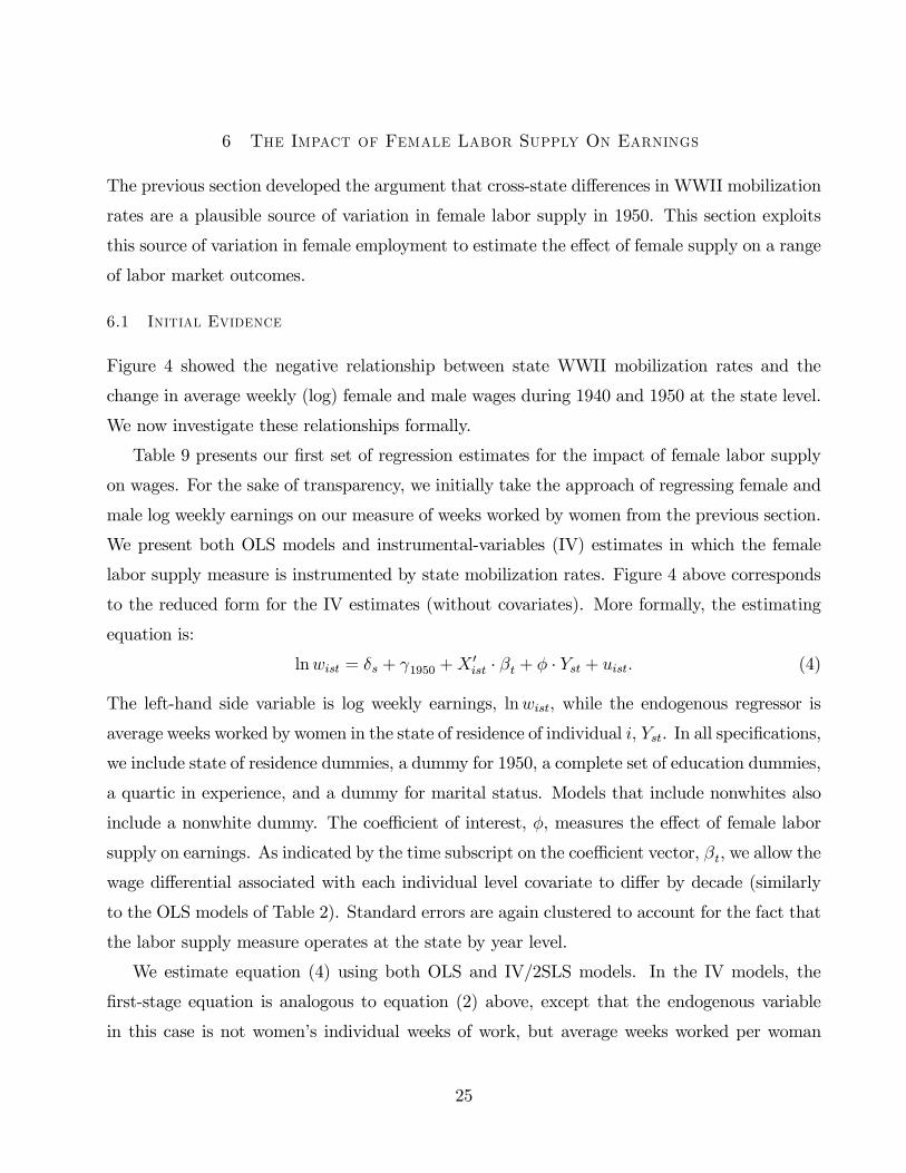
6 The Impact of Female Labor Supply On Earnings

The previous section developed the argument that cross-state differences in WWII mobilization

rates are a plausible source of variation in female labor supply in 1950. This section exploits

this source of variation in female employment to estimate the effect of female supply on a range

of labor market outcomes.

6.1 Initial Evidence

Figure 4 showed the negative relationship between state WWII mobilization rates and the

change in average weekly (log) female and male wages during 1940 and 1950 at the state level.

We now investigate these relationships formally.

Table 9 presents our first set of regression estimates for the impact of female labor supply

on wages. For the sake of transparency, we initially take the approach of regressing female and

male log weekly earnings on our measure of weeks worked by women from the previous section.

We present both OLS models and instrumental-variables (IV) estimates in which the female

labor supply measure is instrumented by state mobilization rates. Figure 4 above corresponds

to the reduced form for the IV estimates (without covariates). More formally, the estimating

equation is:

lnwist = δs + γ1950 +X0ist · βt + φ · Yst + uist. (4)

The left-hand side variable is log weekly earnings, lnwist, while the endogenous regressor is

average weeks worked by women in the state of residence of individual i, Yst. In all specifications,

we include state of residence dummies, a dummy for 1950, a complete set of education dummies,

a quartic in experience, and a dummy for marital status. Models that include nonwhites also

include a nonwhite dummy. The coefficient of interest, φ, measures the effect of female labor

supply on earnings. As indicated by the time subscript on the coefficient vector, βt, we allow the

wage differential associated with each individual level covariate to differ by decade (similarly

to the OLS models of Table 2). Standard errors are again clustered to account for the fact that

the labor supply measure operates at the state by year level.

We estimate equation (4) using both OLS and IV/2SLS models. In the IV models, the

first-stage equation is analogous to equation (2) above, except that the endogenous variable

in this case is not women’s individual weeks of work, but average weeks worked per woman

25

in each state. This first-stage relationship is tabulated directly below the point estimate in

each column. The excluded instrument is the interaction between the 1950 dummy and the

mobilization rate. The exclusion restriction implied by this instrumental-variables strategy is

that differential mobilization rates affect women’s wages across states only through their impact

on female labor supply. Based upon the evidence presented in the previous section, we believe

that this exclusion restriction is plausible.

It is important to bear in mind that estimates of φ do not have a direct structural inter-

pretation in terms of our model in Section 2. As the theory underscores, the impact of female

labor supply on total male and female earnings should depend upon the (log) ratio of female

to male labor supply (as well as the supply of other nonlabor factors). Hence, unless female

labor supply (in OLS or instrumented form) is uncorrelated with male labor supply, we cannot

directly recover the relevant demand and substitution elasticities from estimates of (4). We

therefore view these results as descriptive and adopt a more structural approach in subsequent

tables.

In column 1, we begin with a parsimonious specification which indicates that a 1 week

increase in female labor supply is associated with a 10.7 percent decline in female weekly earn-

ings. Given that women’s labor supply averaged 10.7 weeks in 1940 (Table 1), and assuming

no correlation between (instrumented) female labor supply and male labor supply, this point

estimate would correspond to a female labor demand elasticity of -1.14. In the next column,

we add aggregate measures of female age structure by state to the regression model. These

measures control for the correlation between state mobilization rates and female age struc-

ture.24 Inclusion of age controls reduces the estimated wage impact of female labor supply by

approximately 25 percent to -7.0 percentage points for a 1-week increase, which remains highly

significant. Column 4 adds the interaction between the 1950 dummy and the 1940 aggregate

state measures—share farm, share nonwhite, and average education—thus allowing differential

wage growth in farming, high-minority and low-education states. These interactions reduce

the magnitude of the estimate by one-third and increase the standard error. The lower panel

repeats the results for the white sample with similar results but slightly greater precision. The

negative estimated impact of female labor supply on mean female earnings is in all cases signif-

icant (in the final specifications, at the 10 percent level) and, as suggested by theory, indicates24Female age structure variables measure the share of female state residents ages 14-64 in each of the following

age categories (with one omitted): 14-17, 18-24, 25-34, 45-54, 55-64.

26

that the demand curve for female labor is downward sloping (at least in the short run).

Comparing these IV estimates to the corresponding OLS estimates in the table, which are

typically weakly negative and never significant, suggests that the OLS estimates are likely

biased upward (i.e., towards zero). It appears, not surprisingly, that cross-state variation in

female labor supply during this decade was jointly determined by a combination of demand and

supply shifts. By isolating the component of female employment that is plausibly orthogonal

to demand, our IV estimates show a substantially larger effect of female labor supply on female

earnings.

The subsequent columns of Table 9 present corresponding estimates for male earnings, both

for the full sample and for the white subsample. Contrary to the case of female earnings,

theory does not make strong predictions for male earnings: they should decline if male and

female labor inputs are close substitutes and nonlabor inputs are supplied inelastically to state

labor markets in the short run. In the data, we detect negative effects of female labor supply on

male earnings. All point estimates are highly significant except those in the final specifications

where we control for the interaction between the 1950 dummy and several state aggregate

measures. Interestingly, the estimated effects of female labor supply on male earnings are

consistently 30 to 40 percent smaller in absolute magnitude than the corresponding estimates

for female earnings. This result suggests that female labor supply is an imperfect substitute

for male labor supply, a point which we explore in greater detail below. Once again, the IV

estimates are more negative than the corresponding OLS estimates, consistent with the view

that OLS estimates are biased towards zero due to simultaneity, and that demand for male and

female labor are positively correlated.25

The final columns of Table 9 present wage results estimated separately for male WWII

veterans and non-veterans. These columns provide an important specification test. If aggregate

wage effects for males were driven exclusively by lower wages for veterans, we would be worried

about having primarily detected the adverse effects of war reintegration on veterans’ earnings.26

25Also notice that the negative effects on female wages are unlikely to be accounted by the labor forceparticipation of women with lower earnings capacity (cf. Smith and Ward, 1984). First, as Appendix Table2 shows, marginal labor market participants were relatively highly educated, so there is no compelling reasonto expect that they will be adversely selected on unobserved skills. Second, to rationalize the wage effect weestimate, i.e., over 10 percent decline in wages in response to a 10 percent increase in employment, with theparticipation of less skilled women, we would need the marginal participants to earn negative wages!26Angrist and Krueger (1994) present evidence that WWII veterans were positively selected, and Angrist

(1990) presents evidence that Vietnam Era veterans experienced earnings losses due to foregone civilian expe-rience.

27

The estimates in Table 9 indicate significant negative wage effects of female labor supply for

both non-veterans and veterans. Interestingly, the point estimates for veterans are somewhat

more negative than those of non-veterans. This pattern is consistent with Richard Freeman’s

“Active Labor Market” hypothesis: veterans, as recent labor market (re-)entrants, may have

borne a greater brunt of the wage effects of rising female labor supply.

Appendix Tables 4 estimates models similar to those in Table 9, while controlling for inter-

actions between the 4 Census regions and year, or dropping all Southern state. These results

are quite similar to our baseline estimates, indicating that the negative relationship between

the mobilization-induced changes in female labor supply and changes in earnings is not driven

primarily by Southern states or regional trends.

Given the substantial convergence in regional wage levels that took place among U.S. states

during the 1940s (Wright, 1986), we were also concerned that wage patterns detected in Table

9 might reflect a process of “catching up” whereby agricultural states, which generally had

low-mobilization rates, gained ground on the rest of the nation during this decade. To check

this possibility, we augmented the Table 9 models to control for the 1940 level of wages for

the relevant demographic group (interacted with a 1950 dummy). Appendix Table 5 reports

the results of this exercise. This lagged wage variable is negative and generally significant

indicating that states with initially higher wage levels experienced smaller wage gains during

the decade. The important finding however is that the inclusion of the lagged measure does not

affect our general conclusions. In models without state aggregate measures, point estimates of

the effect of mobilization on wages are lower than the models without lagged wages, but they

are higher when the state aggregate measures are included. In all specifications, the effect of

mobilization-induced changes in female employment on female wages is statistically significant,

and the effect on male wages is always negative, and is significant in all specifications except for

those that control for the interactions between the 1950 dummy and aggregate state measures.27

27The results are also unlikely to be driven by institutional changes taking place in the U.S. labor marketduring this time period. The two major institutional changes of this era are increases in unionization and theimposition, and then removal, of the National War Labor Board (NWLB), which was responsible for approving,and limiting, wage increases.The NWLB and other price controls are unlikely to be responsible for our results. The NWLB, which was

established in January 1942, was dissolved in December 1945, and effectively all wartime price controls werelifted in November 1946 (see Rockoff, 1984), three years before our post-war observations.We have also estimated the key labor supply and wage models in Tables 4 and 9 while controlling for differential

trends in unionization across states during these years (using data from Troy and Sheflin, 1985). Controllingfor unionization has little impact on the findings, and a supplemental table of estimates is available on request.

28

6.2 Using Mobilization Rates to Estimate Elasticities of Demand and Substitution

The wage estimates in Table 9 employ average female weeks as the endogenous regressor.

This approach will lead to correct estimates of the elasticity of demand or substitution only

if (instrumented) female labor supply is uncorrelated with male labor supply. Although this

condition may be satisfied, it would be preferable to exploit exogenous variation in male and

female labor supply simultaneously. Using a single instrument, we cannot separately identify

both sources of variation. We can, however, use the mobilization rate to instrument the (log)

ratio of female to male labor supply in a state. This approach surmounts the problem of treating

male labor supply as exogenous and thereby brings us closer to the specification suggested by

the theoretical model. The equation that we estimate is:

lnwist = δs + γ1950 + fi +X0ist · βgt + χ · ln

µFstMst

¶+ η · fi · ln

µFstMst

¶+ uist, (5)

where the sample now includes all individuals (male and female), fi is a dummy for female,

Fst is total labor supplied by women and Mst is total labor supplied by men in the state of

residence of individual i. As indicated by the super- and subscripts on βgt , each of the individual

and state aggregate control measures included in the model (contained in Xist) is permitted to

impact male and female earnings differentially by gender and decade.

In this equation, there are two coefficients of interest, χ and η. The coefficient χ measures

the direct impact of increases in (relative) female labor supply on male and female earnings,

and η measures the differential effect of female labor supply on female wages. Hence, η is

an estimate of the inverse elasticity of substitution between male and female labor, and the

quantity χ+ η is an estimate of the inverse elasticity of demand for female labor.

In the first four columns of Table 10, we present estimates of equation (5) where the labor

supply measure is constructed as the log ratio of total female to male weeks supplied in each

state and the control variables correspond to those used in the four specifications in Table 9.

First-stage estimates, tabulated in each column, indicate that WWII mobilization substantially

affected relative gender labor supplies. A 10 percent higher mobilization rate is estimated to

have induced a 10 to 20 percent increase in the log ratio of female to male labor supply, an

impact which is always precisely estimated and highly significant.28

28This is a sensible magnitude. For example, an increase in the female to male ratio of labor input from 0.30to 0.35 percent correponds to a 15 log point increase in the this ratio.

29

We next turn to elasticity estimates. The point estimates in the first two rows of Table

10, corresponding to χ and η in equation (5), are consistently negative, economically sizable,

and with few exceptions, highly significant. This set of results confirms the findings above that

the demand curve for female labor is downward sloping and that women are relatively close

substitutes for men.

Summing χ and η to obtain an estimate of the (inverse) elasticity of demand for female labor,

σF , we find that a 10 percent increase in relative female labor supply reduced female wages by

6 to 7 percentage points. These wage effects correspond to an own-labor demand elasticity of

between -1.4 and -1.7 and are therefore slightly larger in magnitude than the “naive” estimates

above. The lower panel of the table presents analogous wage estimates for the subsample of

white female wage earners, for whom we find comparable demand elasticities.

The impact of female labor supply on wages is not uniform between the two genders, how-

ever. As is visible in the second row of Table 10 (and as was suggested by Table 9), the wage

effects of (relative) increases in female labor supply are uniformly more negative for women

than they are for men. A 10 percent increase in female labor supply lowers female wages

relative to male wages by about 3 percentage points. By implication, female and male labor

inputs are highly, but not perfectly, substitutable. In particular, the point estimates for η,

corresponding to the inverse elasticity of substitution σMF , imply a substitution elasticity in

the range of -3, with slightly smaller implied elasticities in the models that include aggregate

state controls. Again, elasticities are similar in Panel B, where estimates are limited to white

males and females.

6.3 Measuring labor supply in efficiency units

As a check on the above results, we also estimate models that replace the aggregate weeks of

labor supply measure with a measure of labor supply calculated in efficiency units following

the approach of Welch (1969). Conceptually, efficiency unit calculations aggregate various

demographic subgroups according to their estimated relative productivities to obtain total labor

supply by gender. To implement this approach, we use the 1940 Census sample to calculate

average weekly earnings for full-time, full-year workers in the following education by race by

gender categories within each state: 5 age categories (13-23, 24-33, 34-43, 44-53, and 54-63); 5

education categories for whites (<8 years, exactly 8 year, between 8 and 12 years, exactly 12

30

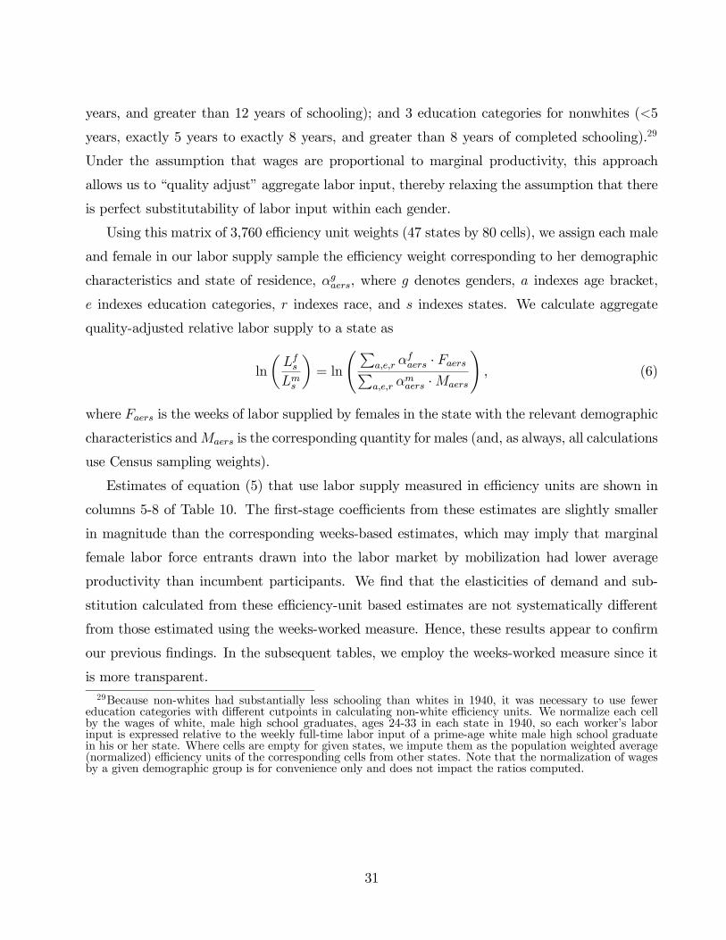
years, and greater than 12 years of schooling); and 3 education categories for nonwhites (<5

years, exactly 5 years to exactly 8 years, and greater than 8 years of completed schooling).29

Under the assumption that wages are proportional to marginal productivity, this approach

allows us to “quality adjust” aggregate labor input, thereby relaxing the assumption that there

is perfect substitutability of labor input within each gender.

Using this matrix of 3,760 efficiency unit weights (47 states by 80 cells), we assign each male

and female in our labor supply sample the efficiency weight corresponding to her demographic

characteristics and state of residence, αgaers, where g denotes genders, a indexes age bracket,

e indexes education categories, r indexes race, and s indexes states. We calculate aggregate

quality-adjusted relative labor supply to a state as

ln

µLfsLms

¶= ln

ÃPa,e,r α

faers · FaersP

a,e,r αmaers ·Maers

!, (6)

where Faers is the weeks of labor supplied by females in the state with the relevant demographic

characteristics andMaers is the corresponding quantity for males (and, as always, all calculations

use Census sampling weights).

Estimates of equation (5) that use labor supply measured in efficiency units are shown in

columns 5-8 of Table 10. The first-stage coefficients from these estimates are slightly smaller

in magnitude than the corresponding weeks-based estimates, which may imply that marginal

female labor force entrants drawn into the labor market by mobilization had lower average

productivity than incumbent participants. We find that the elasticities of demand and sub-

stitution calculated from these efficiency-unit based estimates are not systematically different

from those estimated using the weeks-worked measure. Hence, these results appear to confirm

our previous findings. In the subsequent tables, we employ the weeks-worked measure since it

is more transparent.29Because non-whites had substantially less schooling than whites in 1940, it was necessary to use fewer

education categories with different cutpoints in calculating non-white efficiency units. We normalize each cellby the wages of white, male high school graduates, ages 24-33 in each state in 1940, so each worker’s laborinput is expressed relative to the weekly full-time labor input of a prime-age white male high school graduatein his or her state. Where cells are empty for given states, we impute them as the population weighted average(normalized) efficiency units of the corresponding cells from other states. Note that the normalization of wagesby a given demographic group is for convenience only and does not impact the ratios computed.

31

6.4 Differences between Short-Run and Long-Run Elasticities

As noted in the Introduction and Section 2, the estimates reported in this paper are likely to

correspond to short-run elasticities. In general, it is of great interest to know whether short-

and long-run elasticities differ substantially. Since, as shown in Figure 3, there was only a small

amount of mean reversion in female employment during the 1950s, states with greater WWII

mobilization also had greater female employment in 1960. By exploiting the 20-year changes

between 1940 and 1960, we can investigate whether the short-run impact of increased female

employment is different from its long-run impact. We perform this exercise in Appendix Table

6, by estimating models identical to those in Table 10 except that the two decades we now

cover are 1940 and 1960.

Comparing the first-stage coefficients on the mobilization rate interaction between Table 10

and Appendix Table 7, we see that mobilization had a large effect on the growth of relative

female labor supply not only between 1940 and 1950, but also between 1940 and 1960. For

example, in column 1 of Appendix Table 6, the first-stage coefficient is 2.1, compared to 2.05

in Table 10. However, the standard error is much larger. Thus, not surprisingly, some of the

2SLS estimates will be less precise. Moreover, in models that control for interactions between

the 1960 dummy and share of farmers, nonwhites, and average education in 1940, there is no

first-stage relationship between mobilization and female employment growth between 1940 and

1960.

The models in Appendix Table 6 that do not control for the state aggregates show that the

effect of relative female employment on male wages is broadly comparable between 1940-50 and

1940-60 (columns 1-3 and 5-7). However, the effect of relative female labor supply on male-

female differentials is much weaker for the 20-year state level changes. In fact, the estimates are

essentially zero and the standard error bands easily exclude the short-run elasticity estimate

from Table 10 (though the main effect, which captures the impact on the level of male and

female earnings, is sometimes as large as those in Table 10). This is consistent with the notion

that the long-run relative demand curve for women’s labor is considerably more elastic than

the short-run relative demand curve, or even perhaps perfectly elastic. This could be due to

adjustment of nonlabor inputs that are fixed in the short-run (LeChatelier principle), changes

in technology or in the organization of production favoring women in areas with greater female

employment (Acemoglu, 1998, 2002), or changes in trade patterns that require sufficient time

32

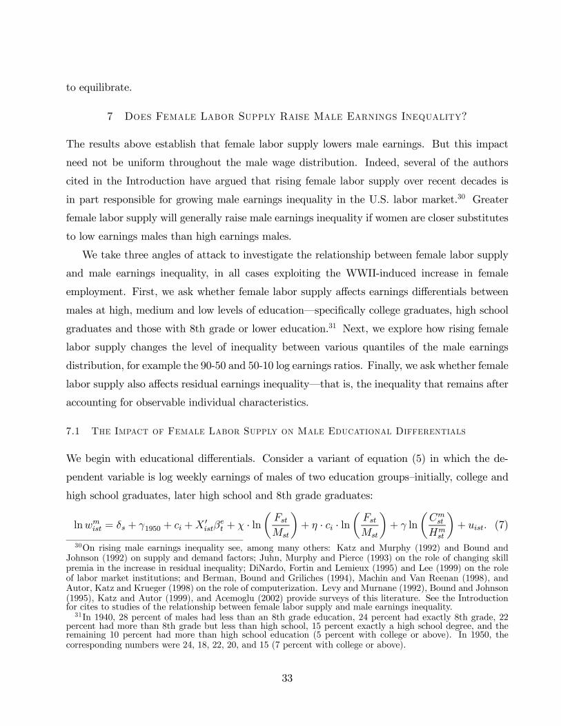
to equilibrate.

7 Does Female Labor Supply Raise Male Earnings Inequality?

The results above establish that female labor supply lowers male earnings. But this impact

need not be uniform throughout the male wage distribution. Indeed, several of the authors

cited in the Introduction have argued that rising female labor supply over recent decades is

in part responsible for growing male earnings inequality in the U.S. labor market.30 Greater

female labor supply will generally raise male earnings inequality if women are closer substitutes

to low earnings males than high earnings males.

We take three angles of attack to investigate the relationship between female labor supply

and male earnings inequality, in all cases exploiting the WWII-induced increase in female

employment. First, we ask whether female labor supply affects earnings differentials between

males at high, medium and low levels of education–specifically college graduates, high school

graduates and those with 8th grade or lower education.31 Next, we explore how rising female

labor supply changes the level of inequality between various quantiles of the male earnings

distribution, for example the 90-50 and 50-10 log earnings ratios. Finally, we ask whether female

labor supply also affects residual earnings inequality–that is, the inequality that remains after

accounting for observable individual characteristics.

7.1 The Impact of Female Labor Supply on Male Educational Differentials

We begin with educational differentials. Consider a variant of equation (5) in which the de-

pendent variable is log weekly earnings of males of two education groups—initially, college and

high school graduates, later high school and 8th grade graduates:

lnwmist = δs + γ1950 + ci +X0istβ

et + χ · ln

µFstMst

¶+ η · ci · ln

µFstMst

¶+ γ ln

µCmstHmst

¶+ uist. (7)

30On rising male earnings inequality see, among many others: Katz and Murphy (1992) and Bound andJohnson (1992) on supply and demand factors; Juhn, Murphy and Pierce (1993) on the role of changing skillpremia in the increase in residual inequality; DiNardo, Fortin and Lemieux (1995) and Lee (1999) on the roleof labor market institutions; and Berman, Bound and Griliches (1994), Machin and Van Reenan (1998), andAutor, Katz and Krueger (1998) on the role of computerization. Levy and Murnane (1992), Bound and Johnson(1995), Katz and Autor (1999), and Acemoglu (2002) provide surveys of this literature. See the Introductionfor cites to studies of the relationship between female labor supply and male earnings inequality.31In 1940, 28 percent of males had less than an 8th grade education, 24 percent had exactly 8th grade, 22

percent had more than 8th grade but less than high school, 15 percent exactly a high school degree, and theremaining 10 percent had more than high school education (5 percent with college or above). In 1950, thecorresponding numbers were 24, 18, 22, 20, and 15 (7 percent with college or above).

33

In this equation, ci is a dummy for whether individual i is a college graduate (the omitted group

being high school graduates), Fst/Mst is relative female labor supply measured in aggregate

weeks worked as above, and Cmst /Hmst is the relative supply of college versus high school male

labor input.32 All covariates are allowed to have different effects on earnings of college and

non-college males and to differ by decade.

The coefficients of interest in this equation are χ and η. The coefficient χ measures the

impact of female labor supply on the earnings of high school graduates, and η gives the effect

of female labor supply on the relative wages of college versus high school graduates. Therefore,

keeping the employment levels of college and high school graduate males constant, we can think

of σfh = 1/χ as the cross-elasticity of demand between female labor and high school gradu-

ates and σfc = 1/ (χ + η) as the cross-elasticity of demand between female labor and college

graduates. The ratio of cross-elasticities of females for high school versus college graduates,

σfhc ≡ σfh/σfc, is therefore (χ+ η) /χ . If σfhc is less than 1, this implies that female labor has

a more (negative) wage impact on high school graduates, so females are closer substitutes to

high school than to college males, and vice versa if σfhc > 1.

Consistent with our previous results, we anticipate that the main effect of female labor

supply on both college and high school wages, χ, is negative. Since relative supplies of male

college versus high school graduates, Cmst /Hmst , should also directly impact the male college/high

school premium, we must either control for this measure or assume that instrumented female

labor supply measure is uncorrelated with it. We implement both approaches below and find

that the choice is not consequential for our results.

While the college/high school wage differential is of great contemporary interest, the vast

majority of males in our 1950 sample (85 percent) had high school or less education, with

the two modes of the distribution found at exactly high school completers (20.3 percent) and

exactly 8th grade completers (18.2 percent). Therefore, it is of interest to ask whether female

labor supply raised or lowered earnings inequality between these groups of males as well. After

estimating equation (7) for the college/high school differential, we perform analogous estimates32In models that use the male college/high school relative supply, college labor supply is the sum of total

weeks worked supplied by college-plus graduates plus half of those supplied by those with some college; highschool labor supply is the sum of weeks worked supplied by high school graduates or less plus half of thosesupplied by those with some college. In models that use the male high school/8th grade relative supply, highschool labor input is the sum of weeks worked supplied by those with high school or more plus half of thatsupplied by those with more than 8th grade and less than high school education; 8th grade is the sum of weeksworked supplied by those those with 8th grade or less, plus half of that supplied by those with more than 8thgrade and less than high school.

34

for the high school/8th grade differential.

Estimates of equation (7) for college and high school graduates, shown in panel A of Table

11, reveal that growth in female labor supply exerts a small positive effect on male college/high

school earnings inequality. A 10 percent increase in female labor supply is predicted to lower

male high school wages by 2.5 to 4 log points while reducing college wages by only 1 to 2.5

percentage points. These point estimates imply a relative cross-elasticity of demand σfhc of 0.4

to 0.6, but this elasticity is imprecisely estimated. This evidence is consistent with the view

that females drawn into the labor force by WWII mobilization were more substitutable for

high school than college educated men (consistent with the characteristics of female labor force

entrants documented in Appendix Table 2). But we cannot reject the hypothesis that women’s

labor supply reduced college and high school wages by equivalent amounts.

This ambiguity does not carry over to the corresponding results for the impact of female

labor supply on the male 8th grade/high school differential. These estimates, found in Panel

B of Table 11, have the opposite sign to and are somewhat larger than those for the male

college/high school wage premium. They are also more precisely estimated. A 10 percent

increase in female labor supply is estimated to reduce male high school relative to 8th grade

earnings by 1.5 to 2.5 percentage points. This relative wage impact is highly significant in

specifications that do not control for state aggregate measures. In models that include these

aggregates, the estimate is of similar magnitude but is less precise. Interestingly, we cannot

reject the hypothesis that female labor supply had no impact on the wages of 8th grade males.

In net, the primary impact of increased female labor supply on male educational inequality

during the 1940s was to lower the wages of male high school graduates relative to more-educated

males, and particularly relative to less-educated males. This suggests that during the WWII

era, females were closer substitutes to males at the middle of the skill distribution than to

males in either of the tails. Given that low-educated males in 1950 were reasonably likely to be

employed in manual occupations, it is plausible that women would indeed be worse substitutes

for them than for their high school graduate brethren. This result stands in some contrast

to Grant and Hamermesh’s (1981) and Topel’s (1994) OLS findings that high-skill women are

strong substitutes for low-skill males. Of course, our findings are from another era and these

substitution parameters need not be fixed over long intervals.

35

7.2 The Impact of Female Labor Supply on the Distribution of Male Earnings

Because women’s labor force entry during the 1940s appears to have raised earnings inequality

between college and high school males while lowering it for high school versus 8th grade educated

males, the net impact on male inequality is–at this point–ambiguous. Educational inequality

is however only one component of earnings differentials, and the total impact of female labor

supply on male inequality could in principle be quite different than its impact on educational

inequality.

To provide a more complete picture of these potential effects, we adopt a less structural

approach. Using observed male earnings distributions and estimated residual male earnings

distributions by state, we define state level inequality metrics as the log difference between

various quantiles of the earnings or residual earnings distribution, such as the 90-50 or 50-10

differential. We then explore whether WWII-induced increases in female labor supply raised

or lowered these inequality measures. To implement this approach, we first estimate standard

wage regressions of the form:

lnwist = δs + γ1950 +X0ist · βt + vist, (8)

where wit is weekly earnings for male i residing in state s in year t. In the “overall inequality”

specification, we include only state dummies and a year main effect. In the “residual inequality”

model, the vectorXist includes a full set of education dummies, a quartic in potential experience,

nonwhite, state of residence, state or country of birth, veteran status, and marital status

dummies, as well as controls for state female age structure by year. A third set of models add

state-level macro controls (share farmer and nonwhite, and average education in 1940). The

fact that βt is indexed by t indicates that returns to these observed characteristics are allowed

to vary by decade. We also briefly look at measures of wage inequality that combine workers

from both genders.

The measures of overall or residual inequality are calculated separately in each state and

year as the difference between the 90th and the 10th (or 50th and 10th, etc.) percentile values

of the corresponding residual distribution, vist, and are denoted by v90−10st etc. Observe that

the residual distribution in the “overall” inequality model is simply the demeaned log earnings

distribution in each state.

We then use these inequality measures as the left-hand side variable in Table 12. The typical

36

regression takes the form:

v90−10st = δs + γ1950 + φ · lnµFstMst

¶+ uist,

where v90−10st is the 90-10 differential, the endogenous regressor, Fst/Mst is again relative female

labor supply (in weeks), and the instrument is the state mobilization rate, ms, interacted with

the 1950 dummy. To move from micro- to macro-data (i.e., from individual Census observations

to state level aggregates) without losing the information provided by the micro-level controls,

we orthogonalize both the instrumental variable and the endogenous regressor with respect

to all of the covariates in Xist to form the state level measures used in the second stage of

estimation.

The first column in Table 12 labeled Mean ∆ provides estimates of mean state-level change

in earnings inequality from 1940 to 1950. The sizable decline in earnings inequality visible in

the table reflects the well-known “Great Compression” studied by Goldin and Margo (1992).

Over the decade of the War, male 90-50 and 50-10 differentials each declined by close to 17 log

points.

The first set of regression estimates in specification 1 examines the state-level relationship

between growth in the log relative supply of female labor input (instrumented with the mobi-

lization rate) and the contemporaneous change in overall state level earnings inequality. The

net impact of female labor supply on male earnings inequality is positive and sizable. A 10

percent increase in female labor input is estimated to widen the 90-10 earnings differential by

5.5 log points, which is highly significant. It is noteworthy that this entire impact occurs in

the upper half of the male earnings distribution. Consistent with our findings for the impact

of female labor supply on the wage gap between middle- and low-education males, increases in

female labor supply appear to cause some compression below the median of the distribution,

though this impact is not significant. An interesting implication of these estimates is that with-

out the WWII-induced increase in female labor force participation the “Great Compression”

would have been even “greater” in the sense that wage inequality among males would have

declined even further between 1940 and 1950.33

33Interestingly and consistent with our findings, Goldin and Margo (1992, p. 27) notice a similar pattern ofwidening inequality in industries with high female employment: “Industries that were female-intensive (cigars,men’s neckwear, woolen and worsted mills) comprise an obvious exception [to the trend of wage compression]...Rather than experiencing a narrowing of the wage structure from the prewar to the wartime or postwar periods,their distributions actually widened.”

37

When we look at the impact of female labor force participation on wage inequality among all

workers (male and female) in Panel C, we find much larger effects. Now a 10 percent increase

in female labor supply widens the 90-10 earnings differential by 1.4 log points. This much

larger effect is not surprising; greater female participation both increases male wage inequality

directly, as we have already established, and also adds more women to the distribution who, at

this time, were paid considerably less than men.

Panel B of the table presents comparable estimates for the white subsample. In this case

the impact of female labor supply on inequality above the median is somewhat less positive

while the impact on inequality below the median is somewhat more negative. This estimate

suggests that female labor supply primarily reduces male earnings at a lower point in the white

male earnings distribution than in the overall earnings distribution, which appears plausible

given the substantial racial disparities in education and earnings in this period.

The subsequent two columns of Panels A and B present estimates of the impact of female

labor supply on residual male inequality. The impact of female labor supply on residual in-

equality is about half as large as the impact on overall inequality, but still sizable. A 10 percent

increase in female labor supply is estimated to raise the male 90-10 earnings differential by

1.5 to 2 log points. The columns numbered (2) present residual estimates in which state level

macro controls (share nonwhite and farm, and average education) are included in the first stage

models. The point estimates are typically less precise than previous estimates.

Overall, the results reported in this section show a substantial effect of female employment

growth on overall and residual inequality among men at midcentury. These results therefore

provide some support to the hypotheses advanced in Fortin and Lemieux (2000) and Topel (1994

and 1997), linking female labor supply to rising male inequality–though distinct from the hy-

potheses of these authors, female labor appears to increase male inequality not by competing

with low-skill males, but by increasing dispersion at the top of the male wage distribution.

Interestingly, the effects we find are large enough to “explain” a large fraction of the recent

increase in male wage inequality as resulting from the concurrent sizable rise in female employ-

ment. This conclusion may be premature, however, for two reasons: first, the education levels

and characteristics of women who increased their labor supply during the decade differ substan-

tially from those of the marginal female labor market participants of today. The structure of

production has also changed substantially since midcentury. Accordingly, substitution elastici-

38

ties we estimate from midcentury may not be directly comparable to the elasticities today. And

second, as noted before, our estimates correspond to short-run elasticities, which may be quite

different from long-run elasticities as the results in Appendix Table 6 suggest.34 To understand

the effect of female employment on the increase in male wage inequality over the past three

decades, the relevant elasticities are long-run elasticities. Work exploiting additional sources of

variation in recent female employment growth is necessary to make progress on uncovering the

links between rising female labor supply and recent changes in the structure of earnings.

8 Conclusion

The epochal rise in female labor force participation is one of the most profound labor market

transformations of the past century. And yet, the economics profession knows relatively little

about the labor market consequences of increased female labor force participation. An empirical

investigation of this issue requires a source of variation in female employment that is orthogonal

to demand for female (and also male) labor.

In this paper, we developed the argument that the differential extent of mobilization for

WWII across U.S. states provides a useful source of variation to identify the effects of women’s

labor force participation on a range of labor market outcomes. We documented that in 1950

women participated more in states where a larger fraction of working-age males served in the

military during the mid-1940s. This differential female labor supply behavior does not seem to

be accounted for by other cross-state differences or possible demand factors, and is not present

in the 1940 data. We interpret this as a shift in female labor supply induced by the mobilization

for the War.

Using this source of variation, we estimate the effect of greater female participation on

female and male wages, returns to education, and wage inequality among men. Our results

indicate more downward sloping demand curves for female labor, and a closer degree of sub-

stitutability between males and females than suggested by OLS estimates, presumably because

OLS regressions are biased towards-zero by simultaneous demand-induced variation in female

employment. We also find that, contrary to a common hypothesis in the literature, women are

not the closest substitutes to the lowest education males, but to high school graduate males (at34In addition, as noted by, among others, Blau and Kahn (1994, 1997), the gender wage gap closed substan-

tially during the 1980s as female employment was rising, suggesting that demand shifts favoring women maybe an important component of the rise in female labor supply.

39

least at midcentury). Nevertheless, because greater female participation increases inequality

in the top half of the male wage distribution, our estimates suggest sizable effects of female

labor force participation on male wage inequality. This finding indicates that a more detailed

investigation of the relationship between the increase in female labor supply and the recent

widening inequality among males would be fruitful.

9 References

Acemoglu, Daron (1998)„ “Why Do New Technologies Complement Skills? Directed Technical

Change and Wage Inequality” Quarterly Journal of Economics, 113(4), November, 1055-1090.

Acemoglu, Daron. (2002), “Technical Change, Inequality and the Labor Market.” Journal

of Economic Literature, 40, March, 7 — 72.

Acemoglu, Daron and Joshua D. Angrist (2000) “How Large Are Human Capital External-

ities? Evidence from Compulsory Schooling Laws” NBER Macro Annual 2000, pp. 9-71.

Angrist, Joshua D. (1990), “Lifetime Earnings and the Vietnam Era Draft Lottery: Evidence

from Social Security Earnings Records.” American Economic Review, 80(3), June, 313 — 336.

Angrist, Joshua D. and Guido W. Imbens. (1995), “Two-Stage Least Squares Estimation of

Average Causal Effects in Models with Variable Treatment Intensity.” Journal of the American

Statistical Association, 90(430), June, 431 — 442.

Angrist, Joshua D. and Alan B. Krueger (1994), “Why Do World War II Veterans Earn

More than non-Veterans?” Journal of Labor Economics, 12(1), January, 74 — 97.

Autor, David H., Lawrence F. Katz and Alan B. Krueger (1998), “Computing Inequal-

ity: Have Computers Changed the Labor Market?” Quarterly Journal of Economics, 113(4),

November, 1169 — 1214.

Autor, David H., Frank Levy and Richard J. Murnane (2001), “The Skill Content of Recent

Technological Change: An Empirical Exploration.” NBER Working Paper No. 8337, June.

Berman, Eli, John Bound and Zvi Griliches (1994), “Changes in the Demand for Skilled La-

bor within U.S. Manufacturing: Evidence from the Annual Survey of Manufacturers” Quarterly

Journal of Economics, 109(2), May, 367-397.

Bernard, Andew B., J. Bradford Jensen and Peter Schott (2001), “Factor Price Equality

and The Economies of the United States.” NBER Working Paper # 8068.

Blanchard, Olivier Jean and Lawrence F. Katz (1992), “Regional Evolutions” Brookings

40

Papers on Economic Activity, 1, 1 - 75.

Blau, Francine and Lawrence Kahn (1994), “Rising Wage Inequality and the U.S. Gender

Gap.” American Economic Review, v84, n2, 23-28.

Blau, Francine and Lawrence Kahn (1997), “Swimming Upstream: Trends in the Gender

Wage Differential in 1980s.” Journal of Labor Economics, v15, n1, 1-42.

Blau, Francine and Lawrence Kahn (2000), “Gender Differences in Pay.” Journal of Eco-

nomic Perspectives, v14, n4, 75-99.

Blau, Francine, Marianne Ferber and Anne Winkler (2002), The Economics of Women,

Men and Work. Upper Saddle River, New Jersey: Prentice Hall.

Bound, John and Harry Holzer (2000, “Demand Shifts, Population Adjustments, and Labor

Market Outcomes during the 1980s.” Journal of Labor Economics, 18(1), 20 - 54.

Bound, John and George Johnson (1992), “Changes in the Structure of Wages in the 1980’s:

An Evaluation of Alternative Explanations.” American Economic Review, v82, n3, 371-92.

Bound, John and George Johnson (1995), “What Are the Causes of Rising Wage Inequality

in the United States?” Federal Reserve Bank of New York Economic Policy Review, v1, n1,

9-17.

Bound, John and Sarah E. Turner (1999), “Going to War and Going to College: Did World

War II and the G.I. Bill Increase Educational Attainment for Returning Veterans?” NBER

Working Paper #7452, December.

Card, David and John DiNardo (2000, “Do Immigrant Inflows Lead to Native Outflows?”

American Economic Review Papers and Proceedings, 90(2), 360 - 367.

Clark, Kim B. and Lawrence H. Summers, (1982) “Labour Force Participation: Timing and

Persistence” Review of Economic Studies, 49(5), 825-844.

DiNardo, John, Nicole Fortin and Thomas Lemieux (1996), “Labor Market Institutions and

the Distribution of Wages, 1973-1992: A Semiparametric Approach.” Econometrica, v64, n5,

1001-44.

Dresser, Laura (1994), “Changing Labor Market Opportunities of White and African-

American Women in the 1940s and the 1980s.” unpublished dissertation, University of Michi-

gan.

Goldin, Claudia (1990), Understanding the Gender Gap: An Economic History of American

Women. Oxford: Oxford University Press.

41

Goldin, Claudia (1991), “The Role of WorldWar II in the Rise of Women’sWork.” American

Economic Review, 81(4), September, 741 — 756.

Goldin, Claudia (1994), “Labor Markets in the Twentieth Century.” NBER Working Paper,

Series on Historical Factors in Long Term Growth #58, June.

Goldin, Claudia and Robert A. Margo (1992), “The Great Compression: The Wage Struc-

ture in the United States at Mid-Century.” Quarterly Journal of Economics, 112, 1-34.

Grant, James H. and Daniel S. Hamermesh (1981), “Labor Market Competition among

Youths, White Women and Others” Review of Economics and Statistics, 63, pp. 354-360.

Hanson, Gordon and Matthew Slaughter, (2002 forthcoming) “Labor Market Adjustment

in Open Economies: Evidence From U.S. States.” Journal of International Economics.

Jaeger, David A. (1997), “Reconciling the Old and New Census Bureau Education Ques-

tions: Recommendations for Researchers.” Journal of Business and Economic Statistics, 15(3),

July, 300-309.

Juhn, Chinhui and Dae Il Kim (1999), “The Effects of Rising Female Labor Supply on Male

Wages.” Journal of Labor Economics, v17, n1, 23-48.

Juhn, Chinhui, Kevin Murphy and Brooks Pierce (1993), “Wage Inequality and the Rise in

Returns to Skill.” Journal of Political Economy, v101, 410-42.

Katz, Lawrence and David Autor (1999), “Changes in the Wage Structure and Earnings

Inequality.” in Orley Ashenfelter and David Card, eds., Handbook of Labor Economics, Volume

3A, Amsterdam: Elsevier-North Holland, 1463-1555.

Katz, Lawrence and Kevin Murphy (1992), “Changes in Relative Wages, 1963-1987: Supply

and Demand Factors.” Quarterly Journal of Economics,107 (1), 35-78.

Krusell, Per, Lee E. Ohanian, José Víctor Ríos-Rull, Gionvanni L. Violante (2000), “Capital-

skill Complimentarity and Inequality: A Macroeconomic Analysis.” Econometrica, 68(5), 1029

— 1053.

Levy, Frank and Richard Murnane (1992), “U.S. Earnings Levels and Earnings Inequality:

A Review of Recent Trends and Proposed Explanations.” Journal of Economic Literature, v30,

n3, 1333-81.

Machin, Stephen and John Van Reenen (1998), “Technology and Changes in Skill Structure:

Evidence from Seven OECD Countries.” Quarterly Journal of Economics, 113 (4), November,

1215 — 1244.

42

Moretti, Enrico (2000), “Estimating the Social Return to Education: Evidence From Lon-

gitudinal and Cross-Sectional Data,” Center for Labor Economics, University of California,

Berkeley, Working Paper No. 22.

O’Neill, June and Solomon Polachek (1993), “Why the Gender Gap in Wages Narrowed in

the 1980s.” Journal of Labor Economics, v11, n1, 205-28.

Samuelson, Paul (1947) The Foundations of Economic Analysis, Cambridge, MA, Harvard

University Press.

Samuelson, Paul (1948) “International Trade and Equalization of Factor Prices” Economics

Journal, 58, 163-84.

Selective Service System (1956), “Special Monographs #1-18.” Washington D.C.: U.S.

Government Printing Office.

James P. Smith and Michael P. Ward (1984), “Women’s Wages and Work in the Twentieth

Century.” Rand, R-3119-NICHD, October.

Stanley, Marcus (1999), “The Mid-Century GI Bills and Higher Education,” Working Paper,

Case Western Reserve University.

Topel, Robert H. (1994), “Wage Inequality and Regional Labour Market Peformance in the

U.S.” in Toshiaki Tachibanaki, ed., Labour Market and Economic Performance: Europe, Japan

and the USA, New York : St. Martin’s Press, 93 — 127.

Topel, Robert H. (1997), “Factor Proportions and Relative Wages: The Supply-Side Deter-

minants of Wage Inequality.” Journal of Economic Perspectives, 11(2), Spring, 55 — 74.

Troy, Leo and Neil Sheflin (1985), U.S. Union Sourcebook: Membership, Finances, Struc-

ture, Directory, New Jersey: IRDIS, Industrial Relations and Information Services.

U.S. Bureau of the Census (1975), “Historical Statistics of the United States.” Washington,

D.C.: U.S. Government Printing Office.

Welch, Finis (1969), “Linear Synthesis of Skill Definition.” Journal of Human Resources,

4(3), 311 — 327.

Welch, Finis (2000), “Growth in Women’s Relative Wages and in Inequality among Men:

One Phenomenon or Two?” American Economic Review, v90, n2, 444-49.

Williams, Constance (1949) “The Status of Women Workers,” in Colston E. Warne et al.,

eds. Labor in Postwar America (New York: Remsen Press, 1949).

Wright, Gavin (1986) Old South, New South (New York: Basic Books).

43

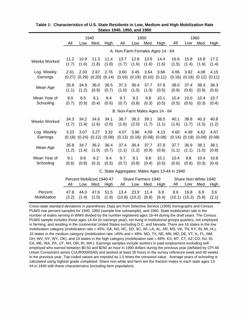
All Low Med. High All Low Med. High All Low Med. High

11.2 10.9 11.3 11.4 13.7 12.8 13.9 14.4 16.6 15.8 16.8 17.2(1.7) (1.6) (1.8) (1.8) (1.7) (1.6) (1.6) (1.6) (1.5) (1.4) (1.6) (1.4)

2.61 2.33 2.67 2.76 3.60 3.45 3.64 3.66 4.06 3.92 4.08 4.15(0.27) (0.29) (0.20) (0.14) (0.16) (0.19) (0.10) (0.11) (0.16) (0.18) (0.12) (0.11)

35.8 34.9 36.0 36.5 37.3 36.4 37.7 37.8 38.0 37.4 38.3 38.3(1.1) (1.2) (0.9) (0.7) (1.0) (1.0) (1.0) (0.5) (0.8) (0.6) (0.9) (0.6)

9.0 8.5 9.1 9.4 9.7 9.2 9.8 10.1 10.4 10.0 10.4 10.7(0.7) (0.9) (0.4) (0.6) (0.7) (0.8) (0.3) (0.5) (0.5) (0.6) (0.3) (0.4)

34.3 34.2 34.6 34.1 38.7 38.3 39.1 38.5 40.1 38.8 40.3 40.8(1.7) (1.4) (1.6) (2.0) (1.6) (2.0) (1.7) (1.1) (1.6) (1.7) (1.5) (1.2)

3.23 3.07 3.27 3.32 4.07 3.96 4.09 4.13 4.60 4.49 4.62 4.67(0.18) (0.24) (0.12) (0.08) (0.13) (0.18) (0.08) (0.08) (0.14) (0.19) (0.09) (0.08)

35.8 34.7 36.2 36.4 37.4 36.4 37.7 37.8 37.7 36.8 38.1 38.1(1.2) (1.4) (1.0) (0.7) (1.1) (1.2) (0.9) (0.6) (1.1) (1.1) (1.0) (0.8)

9.1 8.6 9.2 9.4 9.7 9.1 9.8 10.1 10.4 9.8 10.4 10.8(0.6) (0.8) (0.3) (0.5) (0.7) (0.8) (0.4) (0.5) (0.6) (0.6) (0.3) (0.4)

All Low Med. High All Low Med. High All Low Med. High

47.8 44.0 47.6 51.5 13.4 23.9 11.4 6.9 8.6 16.8 6.9 3.6(3.2) (1.4) (1.0) (1.9) (10.8) (10.2) (8.8) (6.4) (10.1) (15.2) (5.8) (2.1)

Percent Mobilized 1940-47 Share Farmers 1940 Share Non-White 1940

C. State Aggregates: Males Ages 13-44 in 1940

A. Non-Farm Females Ages 14 - 64

Mean Age

Mean Year of Schooling

Mean Year of Schooling

Log Weekly Earnings

Mean Age

B. Non-Farm Males Ages 14 - 64

Percent Mobilization

Weeks Worked

Weeks Worked

Log Weekly Earnings

Table 1: Characteristics of U.S. State Residents in Low, Medium and High Mobilization Rate States 1940, 1950, and 1960

1940 1950 1960

Cross-state standard deviations in parenthesis. Data are from Selective Service (1956) monographs and Census PUMS one percent samples for 1940, 1950 (sample line subsample), and 1960. State mobilization rate is the number of males serving in WWII divided by the number registered ages 18-44 during the draft years. The Census PUMS sample includes those ages 14-64 (in earnings year), not living in institutional groups quarters, not employed in farming, and residing in the continental United States excluding D.C. and Nevada. There are 16 states in the low mobilization category (mobilization rate < 45%: GA, ND, NC, SD, SC, WI, LA, AL, AR, MS, VA, TN, KY, IN, MI, IA,), 15 states in the medium category (mobilization rate ≥45% and < 49%: MO, TX, NE, MN, MD, DE, VT, IL, FL, NM, OH, WV, NY, WY, OK), and 16 states in the high category (mobilization rate ≥ 49%: KS, MT, CT, AZ, CO, NJ, ID, CA, ME, WA, PA, UT, NH, OR, RI, MA.) Earnings samples include workers in paid employment excluding self-employed who earned between $0.50 and $250 an hour in 1990 dollars during the previous year (deflated by CPI All Urban Consumers series CUUR0000SA0) and worked at least 35 hours in the survey reference week and 40 weeks in the previous year. Top coded values are imputed as 1.5 times the censored value. Average years of schooling is calculated using highest grade completed. Share non-white and farm are the fraction males in each state ages 13-44 in 1940 with these characteristics (including farm population).

1940 - 90 1970 - 90 1940 - 60 1940 - 50 1940 - 90 1970 - 90 1940 - 60 1940 - 50(1) (2) (3) (4) (1) (2) (3) (4)

0.008 -0.004 0.016 -0.006 -0.008 -0.011 -0.001 -0.008(0.005) (0.004) (0.008) (0.011) (0.003) (0.003) (0.006) (0.006)

R2 0.88 0.70 0.74 0.64 0.89 0.67 0.74 0.58

n 338,322 417,019 152,428 78,094 545,483 694,219 413,793 213,966

1940 - 90 1970 - 90 1940 - 60 1940 - 50 1940 - 90 1970 - 90 1940 - 60 1940 - 50(1) (2) (3) (4) (1) (2) (3) (4)

-0.010 -0.010 -0.004 -0.003 0.016 -0.017 0.033 0.037(0.004) (0.004) (0.006) (0.006) (0.016) (0.013) (0.048) (0.012)

R2 0.83 0.65 0.71 0.55 0.64 0.92 0.63 0.98

n 274,238 376,878 143,031 60,445 94 94 94 94

Weeks Worked per Woman

A. Female Weekly Earnings B. Male Weekly Earnings

Weeks Worked per Woman

C. Male College/High School Differential D. Male 90-10 Differential

Table 2. OLS Estimates of Impact of Female Labor Supply on Earnings1940 - 1990 at Various Time Intervals

Dependent Variable: Log Weekly Earnings of Full-Time Workers

Sample: All Full Time Workers

Standard errors in parentheses account for clustering on state and year of observation. Each coefficient in Panels A - C is from a pooled microdata regression of the independent variable of interest from the two relevant decades regressed on average female weeks worked by state. Additional controls include a quartic in potential experience, a year main effect, a constant, and dummies for: non-white, age, marital status, state/country of birth, state of residence, and years of completed education. All individual demographic variables, aside from state of residence/birth, are also interacted with a year dummy. Birthplace dummies correspond to state of birth (if U.S. born) or German, Italian, Japanese, Other European, Other Asian, African, Latin American, and Other. Models in Panel C are analogous to those in Panels A and B, but are limited to those with exactly a college or high school degree and all individual level covariates are additionally interacted with a college graduate dummy. In these specifications, female weeks worked is both entered directly and interacted with a college graduate dummy, with the coefficient on the interaction reported above. Panel D tabulates separate regressions of estimated state level log 90-10 earnings ratio of male full-time weekly earners on weeks worked per female state resident, state dummies, a year dummy, and a constant. All education values for years 1940-1970 are coded as highest grade completed. Following the recommendations of Jaeger (1997), we define high school graduates in 1990 as those with twelve years of completed schooling, a GED, or a high school diploma and we define high school graduates in 1970 as those with exactly 12 years of completed schooling and no additional uncompleted schooling. Data are drawn from Census PUMS one percent samples (1950 sample line subsample) for years 1940-1970 and 1990. 1980 data is drawn from Census 5 percent sample using a randomly drawn 20 percent subsample. Samples include those ages 14 - 64 in earnings year, not living in institutional group quarters, residing in mainland U.S. state excluding Nevada and the District of Columbia with non-farm paid employment in survey reference week (excluding self-employed) and positive earnings in previous calendar year who earned between $0.50 and $250 an hour in 1990 dollars during the previous year (deflated by CPI All Urban Consumers series CUUR0000SA0) and worked at least 35 hours in the survey week and 40 weeks in the previous year. Top coded earnings values are imputed as 1.5 times the censored value.

Mean(sd) (1) (2) (3) (4) (5) (6) (7) (8) (9) (10) (11) (12) (13)

0.15 -0.17 -0.16 -0.17 -0.17 -0.23 -0.26 -0.22 -0.17 -0.16 -0.17 -0.20 -0.23 -0.25(0.11) (0.05) (0.04) (0.03) (0.04) (0.06) (0.04) (0.04) (0.05) (0.04) (0.05) (0.04) (0.04) (0.04)

0.10 0.00 -0.07 -0.03 -0.38 0.04 -0.03 -0.03 0.02 -0.03 -0.01 0.02(0.11) (0.05) (0.04) (0.06) (0.27) (0.05) (0.05) (0.06) (0.06) (0.06) (0.06) (0.05)

8.89 0.02 0.01 0.01 0.01 0.03 0.01 0.01 0.01 0.01 0.01 0.02(0.71) (0.01) (0.01) (0.01) (0.01) (0.01) (0.01) (0.01) (0.01) (0.01) (0.01) (0.01)

0.42 0.22 0.73 -0.36 0.38(0.03) (0.34) (0.24) (0.24) (0.33)

0.31 0.09 0.38 -0.84 -0.03(0.01) (0.49) (0.48) (0.53) (0.54)

0.007 -3.15 -1.88 -2.19 -1.16(0.006) (0.90) (0.55) (0.74) (0.76)

0.010 1.67 0.00(0.012) (0.52) (0.42)

0.50 -0.09 -0.22(0.03) (0.18) (0.13)

0.47 0.07 0.00(0.03) (0.13) (0.12)

0.19 0.06 0.13(0.05) (0.07) (0.09)

0.20 0.51 0.40 0.42 0.46 -0.19 0.42 0.42 0.49 0.42 0.42 0.94 0.15(0.34) (0.01) (0.05) (0.08) (0.12) (0.27) (0.07) (0.08) (0.08) (0.09) (0.07) (0.25) (0.34)

R2 0.78 0.57 0.58 0.58 0.39 0.68 0.67 0.58 0.61 0.58 0.60 0.62 0.70

Yes Yes Yes Yes No Yes Yes Yes Yes Yes Yes Yes Yes

Share Ages 25-34

Share German

Southern States

Intercept

Table 3. Determinant of State Level WWII Mobilization RatesDependent Variable: Mobilization Rate

Share Italian or Japanese

Draft Boards/ Pop (1000/s)

Share Fathers

Avg Completed

Share Farm

Share Non-white

Share Married

Share Ages 13-24

Standard errors are in parenthesis for regression models. Standard deviations are in parentheses for column of means. Columns 1 - 13 contain regression estimates of state WWII mobilization rates (mean 0.475, standard deviation 0.032) on listed variables. Sample includes observations for 47 U.S. states excluding Hawaii, Alaska, Nevada, and the District of Columbia. Regressions are weighted by male population ages 13 - 44 in each state from the 1940 Census PUMS. State mobilization rate is the number of males who served in WWII divided by the number registered males ages 18-44 during 1940 to 1945 from Selective Service (1956) monographs. The Percent Farm, Non-white, Married, and Average Education variables are state averages for these variables for males ages 13 - 44 calculated from the 1940 Census PUMS. Percent German, Italian, and Japanese are the fraction of male state residents ages 13-44 born in these countries. Percent Fathers is the fraction of women ages 14 - 44 with any children in 1940 (a proxy for paternity). Draft Boards per Population is the number of state local draft boards divided by the number of men registered in each state (in thousands) ages 18 - 44 during 1940 to 1945. Southern states excluded from column 5 include VA, AL, AR, FL, GA, LA, MS, NC, SC, TX,KY, MD, OK, TN, WV.

(1) (2) (3) (4) (5) (1) (2) (3) (4) (5)

Mobilization Rate x 1950 13.89 9.59 9.06 10.22 8.28 11.17 10.42 9.85 10.64 8.51(1.78) (2.38) (2.35) (2.61) (2.39) (1.89) (2.02) (2.05) (2.65) (2.37)

2.04 1.45 1.74 1.04(1.13) (1.13) (1.08) (1.05)

-2.04 0.70 -1.96 -0.72(1.24) (1.86) (1.15) (1.37)

0.51 0.52(0.18) (0.16)

R2 0.01 0.17 0.17 0.17 0.17 0.01 0.18 0.18 0.18 0.18n

Age & Marital Status No Yes Yes Yes Yes No Yes Yes Yes Yes

State of Birth No No Yes Yes Yes No No Yes Yes Yes

B. White Females

Table 4. Impact of World War II Mobilization Rates on Female Labor Supply 1940 - 1950Dependent Variable: Annual Weeks Worked

A. All Females

1940 Male Average Years of Education x 1950

530,026

1940 Male Fraction Farmers x 1950

1940 Male Fraction Non-white x 1950

585,745

Standard errors in parenthesis account for clustering on state of residence and year of observation. Each column is from a separate pooled 1940 and 1950 microdata regression of weeks worked by female state of residence on WWII state mobilization rate interacted with a 1950 dummy, state of residence dummies, a non-white dummy (where relevant), a year main effect, and a constant. Specifications in columns 2 - 5 also include dummies for marital status and years of age. Specifications in columns 3 - 5 contain state/country of birth dummies. All individual demographic variables, aside from state of residence/birth, are also interacted with a 1950 dummy for columns 2-5. As indicated, models also control for state fraction farmers, non-white, and average years of completed schooling among males ages 13 - 44 in 1940 in women's state of residence (each interacted with a 1950 dummy). Data are from Census PUMS one percent samples for 1940 and 1950 (sample line sub-sample) and include females ages 14 - 64, not living in institutional group quarters, not in farm employment, and residing in mainland U.S. states excluding Nevada and District of Columbia. State mobilization rate is assigned by female state of residence.

(1) (2) (3) (4) (5) (6) (7) (8) (9) (10)

8.44 8.24 10.90 9.90 8.77 10.61 7.88 10.87 9.06 8.86(2.35) (2.12) (2.31) (2.43) (2.50) (2.52) (2.41) (2.46) (2.33) (2.29)

2.86 5.82 -5.57 -3.56 0.60 -2.45 -51.81 -12.66 -5.27 0.45(7.23) (6.92) (3.86) (6.42) (3.89) (2.09) (61.05) (5.71) (4.12) (1.24)

R2 0.17 0.17 0.17 0.17 0.17 0.17 0.17 0.17 0.17 0.17

8.11 7.79 5.97 7.78 8.48 8.45 8.30 7.11 8.42 10.56(2.44) (2.59) (2.47) (2.32) (2.63) (2.30) (2.35) (2.46) (2.62) (2.48)

-2.87 -7.25 -10.26 -15.74 1.14 3.88 -19.08 -13.84 -0.57 2.29(8.68) (8.49) (5.20) (6.80) (8.02) (2.60) (73.70) (7.52) (3.69) (1.19)

R2 0.17 0.17 0.17 0.17 0.17 0.17 0.17 0.17 0.17 0.17

n

Table 5. Impact of World War II Mobilization Rates on Female Labor Supply 1940 - 1950Controlling for the Fraction Males in Occupations in 1940

Dependent Variable: Female Annual Weeks Worked by State

Mobilization Rate x 1950

1940 Occupation Share Controlled

Prof/ Tech

Mngrs Clerks SvcsLabor-

ers

585,745

B. Controlling for 1940 Share Farm and Non-White, and Average Years of Education

A. Main specification

Mobilization Rate x 1950

1940 Male Occ. Share x 1950

1940 Male Occ. Share x 1950

Defense Indust.

Sales CraftOper-atives

Svcs/ Private

Standard errors in parenthesis account for clustering on state of residence and year of observation. Each column is from a separate pooled 1940 and 1950 microdata regression of weeks worked by female state of residence on WWII state mobilization rate interacted with a 1950 dummy, the fraction of males in the listed occupational (industry) category in 1940 interacted with a 1950 dummy, a year main effect, a constant, and dummies for: non-white (where relevant), age, marital status, state of residence, and state/country of birth. All individual demographic variables, aside from state of residence/birth, are also interacted with a 1950 dummy. Models in panel B also control for state fraction farmers, non-white, and average years of completed schooling among males ages 13 - 44 in 1940 in women's state of residence (each interacted with a 1950 dummy.) Data are from Census PUMS one percent samples for 1940 and 1950 (sample line sub-sample) and include females ages 14 - 64 not living in institutional group quarters, not in farm employment, and residing in mainland U.S. states excluding Nevada and District of Columbia. State mobilization rate is assigned by female state of residence. Occupation and Industry codes correspond to major (1-digit) occupational and industry categories. The defense industries correspond to IPUMS 1950 industry codes 326 - 388.

(1) (2) (3) (4) (5) (6) (1) (2) (3) (4) (5) (6)16.65 13.73 11.38 15.78 13.19 11.42 14.60 -17.47 1.48 10.93 -17.00 -0.04(6.15) (6.11) (4.42) (5.38) (5.49) (3.97) (13.17) (15.03) (12.82) (12.23) (13.98) (11.94)

3.11 2.61 2.20 2.65 2.19 1.87 3.27 -2.50 0.91 2.66 -2.45 0.65(1.39) (1.21) (1.07) (1.30) (1.11) (1.01) (1.82) (2.53) (1.66) (1.75) (2.45) (1.65)

0.34 0.38 0.40 0.36 0.39 0.41 0.66 1.01 0.80 0.65 0.96 0.77(0.14) (0.17) (0.14) (0.14) (0.15) (0.13) (0.38) (0.37) (0.37) (0.37) (0.36) (0.36)

0.49 0.21 0.56 0.27 0.69 0.41 0.73 0.44(0.14) (0.15) (0.14) (0.15) (0.15) (0.15) (0.14) (0.15)

-0.04 -0.30 0.04 -0.22 -0.04 -0.23 -0.01 -0.20(0.23) (0.25) (0.22) (0.25) (0.21) (0.22) (0.21) (0.21)

-1.73 -1.36 -1.83 -1.33 -1.96 -1.30 -2.03 -1.30(0.39) (0.46) (0.39) (0.46) (0.38) (0.41) (0.38) (0.41)

P-value: 1st Stage 0.00 0.00 0.00 0.00 0.00 0.00 0.00 0.00 0.00 0.00 0.00 0.00

n

Dependent Variable: Annual Weeks Worked

A. Females B. Males

Table 6: Instrumental Variables Estimates of the Impact of World War II Mobilization Rateson Female Labor Supply 1940 - 1950

1940 Male Fraction German x 1950

All

479,867 441,343

1940 Male Fraction Farmers x 1950

1940 Male Avg. Education x 1950

1st Stage Results 1st Stage Results

585,745 530,026

White

1940 Male Fraction 13-24 x 1950

1940 Male Fraction 25-34 x 1950

All

Mobilization Rate x 1950

White

Standard errors in parenthesis account for clustering on state of residence and year of observation. Each column is from a separate pooled 1940 and 1950 microdata 2SLS regression of weeks worked by female state of residence on instrumented WWII state mobilization rate interacted with a 1950 dummy, a year main effect, a constant, and dummies for: non-white (where relevant), age, marital status, state of residence, and state/country of birth. All individual demographic variables, aside from state of residence/birth, are also interacted with a 1950 dummy. Instruments used in the first stage of these models are the fraction of males ages 13-44 in 1940 who are of German birth or who are in the listed age categories (each interacted with a 1950 dummy). Models also control for state fraction farmers and average years of completed schooling among males ages 13 - 44 in 1940 in women's state of residence (interacted with a 1950 dummy). Data are from Census PUMS one percent samples for 1940 and 1950 (sample line sub-sample) and include those ages 14 - 64, not living in institutional group quarters, not in farm employment, and residing in mainland U.S. states excluding Nevada and District of Columbia. State mobilization rate is assigned by state of residence.

(1) (2) (3) (4) (5) (6) (7) (8)

9.06 8.28 12.21 6.54 9.85 8.51 11.28 6.34(2.35) (2.39) (2.98) (2.31) (2.05) (2.37) (2.97) (2.40)

R2 0.17 0.17 0.17 0.19 0.18 0.18 0.18 0.20

0.019 0.184 0.282 0.148 0.063 0.174 0.253 0.130(0.076) (0.072) (0.079) (0.080) (0.069) (0.071) (0.080) (0.081)

R2 0.17 0.17 0.17 0.19 0.18 0.18 0.18 0.20

n 585,745 585,745 585,745 410,794 530,026 530,026 530,026 393,820

(1) (2) (3) (4) (5) (6) (7) (8)

-3.85 2.70 0.09 3.66 -7.25 2.15 0.39 3.56(1.95) (2.15) (2.43) (2.11) (1.81) (1.95) (2.23) (1.86)

R2 0.14 0.14 0.14 0.16 0.15 0.15 0.15 0.17

0.044 -0.009 -0.017 0.032 -0.057 -0.006 0.002 0.035(0.054) (0.069) (0.071) (0.073) (0.049) (0.067) (0.064) (0.069)

R2 0.13 0.13 0.13 0.14 0.14 0.14 0.14 0.15

n 683,976 683,976 683,976 480,545 615,590 615,590 615,590 449,275

Region x 1950 No No Yes No No No Yes No

Excluding South No No No Yes No No No Yes

Yes Yes

All White

Weeks Worked

Any Weeks Worked

YesYesNo Yes NoYesFraction Farm / Non-white/ Avg Ed

A. 1940 - 1950

Weeks Worked

Any Weeks Worked

B. 1950 - 1960

All White

Coefficient on Mobilization Rate Variable x 1960

Coefficient on Mobilization Rate Variable x 1950

Table 7. Impact of World War II Mobilization Rates on Female Labor Supply1940 - 1950 and 1950 - 1960

Dependent Variable: Female Weeks Worked

Standard errors in parenthesis account for clustering on state of residence and year of observation. Each column is from a separate pooled 1940 - 1950 or 1950 - 1960 microdata regression of individual weeks worked on WWII state mobilization rate interacted with a 1950 or 1960 dummy (in Panels A and B respectively), a year main effect, a constant, and dummies for: non-white (where relevant), marital status, age, state of residence, and state/country of birth. All individual demographic variables, aside from state of residence/birth, are also interacted with a 1950 or 1960 dummy. As indicated, models also control for state fraction farmers, non-white, and average education among males ages 13 - 44 in 1940 in women's state of residence (each interacted with a 1950 dummy.) State mobilization rate is assigned by female state of residence. Data are from Census PUMS one percent samples for 1940, 1950 (sample line sub-sample) and 1960, and include females ages 14 - 64, not living in institutional group quarters, not in farm employment, and residing in mainland U.S. state excluding Nevada and District of Columbia. Weeks worked for 1960 is calculated using the midpoint of the intervalled weeks worked. Any weeks worked is defined as weeks worked greater than zero. Region x 1950 dummies refer to 4 main Census geographic regions. Southern states excluded from columns 4 and 8 are VA, AL, AR, FL, MS, NC, SC, TX, KY, MD, OK, TN, and WV.

(1) (2) (3) (4) (5) (6) (7) (8) (9)

Mobilization Rate x 1950 4.09 5.33 5.09 -5.50 -5.41 7.79 -2.82 0.53 -10.63(5.96) (5.63) (5.69) (7.56) (8.01) (6.51) (9.27) (5.40) (7.35)

2.30 2.33 2.50 2.40(1.34) (1.47) (1.88) (1.35)

-9.15 -9.32 -10.59 -7.52(1.24) (2.66) (3.51) (1.40)

-0.03 -0.21 0.29(0.47) (0.59) (0.27)

R2 0.02 0.35 0.35 0.35 0.36 0.36 0.36 0.34 0.34n

(1) (2) (3) (4) (5) (6) (7) (8) (9)

Mobilization Rate x 1950 0.46 4.09 3.60 -6.56 -6.56 7.37 -4.15 -4.03 -10.84(5.98) (5.34) (5.43) (7.12) (7.59) (6.46) (9.02) (4.71) (6.64)

1.97 1.97 1.97 2.74(1.27) (1.41) (1.86) (1.39)

-9.11 -9.11 -10.56 -6.50(1.21) (1.46) (2.04) (0.85)

0.00 -0.19 0.36(0.44) (0.57) (0.23)

R2 0.02 0.36 0.36 0.36 0.36 0.37 0.37 0.35 0.35n

Age & Marital Status No Yes Yes Yes Yes Yes Yes Yes Yes

State of Birth No No Yes Yes Yes No Yes No Yes

1940 Male Fraction Farmers x 1950

366,737441,343

442,606

1940 Male Fraction Non-white x 1950

All

406,591

1940 Male Avg Years of Schooling x 1950

479,867

Table 8. Impact of World War II Mobilization Rates on Male Labor Supply 1940 - 1950Dependent Variable: Annual Weeks Worked

A. All MalesNon-Vets VetsAll

1940 Male Fraction Non-white x 1950

Non-Vets Vets

1940 Male Fraction Farmers x 1950

397,338

1940 Male Avg Years of Schooling x 1950

B. White Males

Standard errors in parenthesis account for clustering on state of residence and year of observation. Each column is from a separate pooled 1940 - 1950 microdata regression of individual weeks worked on WWII state mobilization rate interacted with a 1950 dummy, a year main effect, a constant, and dummies for non-white (where relevant) and state of residence. Specifications in columns 2 - 5 add dummies for married and age. Specifications in columns 3 - 5 add state/country of birth dummies. Columns 6 - 9 include all 1940 males and only WWII Veterans or Non-Veterans in 1950 as noted. All individual demographic variables, aside from state of residence/birth, are also interacted with a 1950 dummy for columns 2-9. As indicated, models also control for state fraction farmers, non-white, and average education among males ages 13 - 44 in 1940 in male's state of residence (each interacted with a 1950 dummy). State mobilization rate is assigned by male state of residence.

(1) (2) (3) (4) (5) (6) (7) (8) (9) (10) (11) (12)

IV - Weeks Worked per Woman -0.107 -0.103 -0.103 -0.068 -0.062 -0.060 -0.061 -0.023 -0.046 -0.025 -0.087 -0.014(0.024) (0.024) (0.023) (0.041) (0.012) (0.013) (0.014) (0.019) (0.011) (0.018) (0.020) (0.022)

13.21 13.03 13.02 9.35 13.36 13.11 13.10 9.76 13.08 9.72 13.45 10.16(1.61) (2.39) (2.39) (2.70) (1.80) (2.37) (2.37) (2.67) (2.36) (2.65) (2.52) (2.81)

OLS -Weeks Worked per Woman -0.006 -0.006 -0.007 0.007 -0.009 -0.008 -0.008 0.004 -0.004 0.004 -0.015 0.005(0.011) (0.010) (0.010) (0.006) (0.006) (0.006) (0.006) (0.003) (0.005) (0.003) (0.008) (0.006)

n

(1) (2) (3) (4) (5) (6) (7) (8) (9) (10) (11) (12)

IV - Weeks Worked per Woman -0.124 -0.108 -0.108 -0.072 -0.080 -0.070 -0.071 -0.021 -0.052 -0.024 -0.102 -0.014(0.029) (0.025) (0.025) (0.038) (0.018) (0.015) (0.015) (0.017) (0.012) (0.016) (0.024) (0.020)

10.22 11.70 11.68 11.20 10.23 11.66 11.65 11.44 11.70 11.42 11.82 11.74(1.81) (2.15) (2.14) (2.72) (1.90) (2.17) (2.16) (2.73) (2.17) (2.72) (2.26) (2.82)

OLS -Weeks Worked per Woman -0.004 -0.012 -0.012 -0.001 -0.006 -0.009 -0.009 0.000 -0.005 0.000 -0.016 0.001(0.011) (0.010) (0.010) (0.007) (0.006) (0.006) (0.006) (0.003) (0.005) (0.003) (0.009) (0.005)

nFemale Age Structure No Yes Yes Yes No Yes Yes Yes Yes Yes Yes Yes

State of Birth No No Yes Yes No No Yes Yes Yes Yes Yes Yes

Fraction Farm/Non-white/Avg Ed No No No Yes No No No Yes No Yes No Yes

162,484

1st Stage Coefficient(Mobilization Rate x 1950)

69,335 198,385 178,163

174,494

B. Full-Time Weekly Earnings: WhitesFemales Males Male Non-Vets Male Veterans

1st Stage Coefficient(Mobilization Rate x 1950)

78,094 213,966 192,256

Table 9. IV Specifications: Impact of Female Labor Supply on Female and Male Earnings 1940 - 1950Dependent Variable: Log Weekly Earnings

A. Full-Time Weekly Earnings: AllFemales Males Male Non-Vets Male Veterans

Standard errors in parentheses account for clustering on state and year of observation. Each column is from a separate pooled 1940 - 1950 microdata regression of log weekly earnings on weeks worked per female by state of residence. All regressions control for state of residence, a year main effect, education, a quartic in potential experience, a constant, and dummies for non-white (where relevant), marital status, and WWII Veteran (for males). All individual demographic variables, aside from state of residence/birth, are interacted with a 1950 dummy. All columns except 1 and 5 control for female age structure (the first two age categories in five year increments, the remaining four in ten year increments over age range 14 - 64). As indicated, models control for state/country of birth and fraction farmers, non-whites, and average education of males ages 13 - 44 in 1940 by state of residence (each interacted with a 1950 dummy). Columns 9 - 12 contain all males in 1940 and only WWII Veterans or WWII non-Veterans in 1950 as noted. Weeks worked per woman is calculated for all non-farm female state residents ages 14 - 64. In OLS regressions, this variable is treated as exogenous. In IV regressions, it is instrumented by state WWII mobilization rate interacted with a 1950 dummy variable. All individual and aggregate controls are included in first stage models. The first stage coefficient and standard error on the mobilization rate variable are given below the regression. Data are from Census PUMS one percent samples (1950 limited to sample line observations) and include those ages 14 - 64, in paid non-farm employment in survey reference week (excluding self-employed), with positive earnings in previous calendar year, who earned between $0.50 and $250 an hour in 1990 dollars (deflated by CPI All Urban Consumers series CUUR0000SA0), who worked at least 35 hours in the survey week and 40 weeks in the previous year, did not live in institutional group quarters, and resided in mainland U.S. states excluding Nevada and the District of Columbia.

(1) (2) (3) (4) (5) (6) (7) (8)

ln(LSFemale/LSMale) -0.390 -0.386 -0.391 -0.226 -0.471 -0.440 -0.446 -0.197(0.075) (0.074) (0.076) (0.190) (0.098) (0.092) (0.095) (0.165)

-0.328 -0.278 -0.272 -0.354 -0.432 -0.332 -0.324 -0.309(0.115) (0.105) (0.099) (0.182) (0.157) (0.126) (0.119) (0.161)

2.05 2.03 2.03 1.09 1.67 1.77 1.77 1.24(0.19) (0.25) (0.25) (0.25) (0.19) (0.24) (0.24) (0.29)

Implied Female Demand σF -1.39 -1.51 -1.51 -1.73 -1.11 -1.30 -1.30 -1.98

Implied M/F Substition σM/F -3.05 -3.60 -3.68 -2.83 -2.32 -3.02 -3.08 -3.24

p-value of H0: (σF)-1 = 0 0.00 0.00 0.00 0.08 0.00 0.00 0.00 0.08

n

(1) (2) (3) (4) (5) (6) (7) (8)

ln(LSFemale/LSMale) -0.513 -0.463 -0.469 -0.254 -0.527 -0.473 -0.480 -0.237(0.107) (0.089) (0.092) (0.200) (0.113) (0.096) (0.099) (0.185)

-0.315 -0.264 -0.254 -0.421 -0.331 -0.277 -0.266 -0.380

(0.126) (0.117) (0.116) (0.191) (0.139) (0.124) (0.122) (0.170)

1.56 1.75 1.75 1.14 1.51 1.70 1.70 1.22(0.19) (0.22) (0.22) (0.30) (0.20) (0.24) (0.24) (0.34)

Implied Female Demand σF -1.21 -1.38 -1.38 -1.48 -1.17 -1.33 -1.34 -1.62

Implied M/F Substition σM/F -3.18 -3.78 -3.94 -2.37 -3.02 -3.61 -3.76 -2.63

p-value of H0: (σF)-1 = 0 0.00 0.00 0.00 0.06 0.00 0.00 0.00 0.06

n

Female Age Structure No Yes Yes Yes No Yes Yes Yes

State of Birth No No Yes Yes No No Yes Yes

Farm/Non-white/Avg Ed No No No Yes No No No Yes

Table 10. Impact of Female Labor Supply on Female/Male Earnings Differential 1940 - 1950Dependent Variable: Log Weekly Earnings

A. Full-Time Weekly Earnings: AllLabor Supply Measured

in WeeksLabor Supply Measured

in Efficiency Units

ln(LSFemale/LSMale)x Female

292,060

B. Full-Time Weekly Earnings: White

1st Stage Coefficient(Mobilization Rate x 1950)

Labor Supply Measuredin Weeks

Labor Supply Measuredin Efficiency Units

267,720

ln(LSFemale/LSMale)x Female

1st Stage Coefficient(Mobilization Rate x 1950)

Standard errors in parentheses account for clustering on state and year of observation. Each column is from a separate pooled 1940 - 1950 microdata regression of log weekly male and female earnings on the log ratio of female to male non-farm labor supply measured in weeks (columns 1-4) or efficiency units (columns 5 - 8). All models include controls for veteran status, nonwhite, marital status, education, a quartic in potential experience, (each interacted with a female dummy and a 1950 dummy), state of residence, and a year main effect. As indicated, models control for state female age structure and state/country of birth, and state fraction farmers, non-whites, and average education among males ages 13 - 44 in 1940 (each interacted with a 1950 dummy.) All variables are interacted with a female dummy. Log of (female/male) labor supply measure is calculated for all non-farm state residents ages 14 - 64. This measure and its interaction with a female dummy are instrumented by state WWII mobilization rate and its interaction with a female dummy. The first stage coefficient on the mobilization rate main effect is tabulated below each regression. All individual and aggregate controls are included in first stage models. See text for details of the efficiency unit measure used in columns 5 - 8.

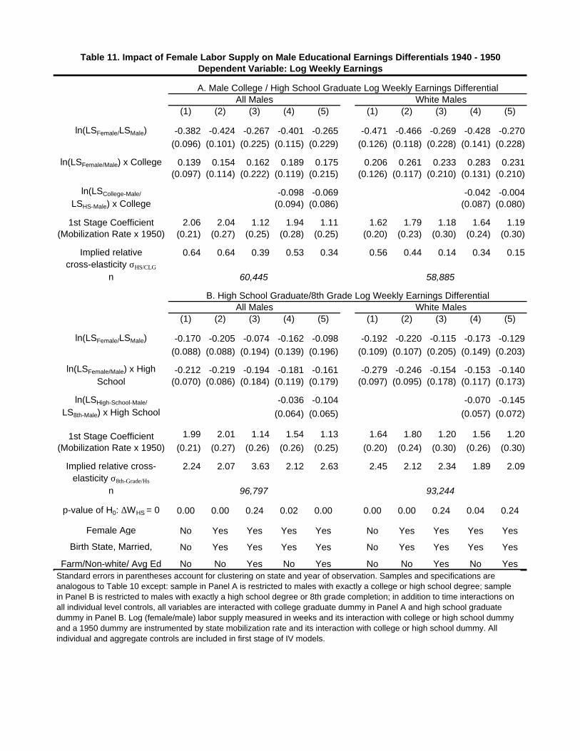
(1) (2) (3) (4) (5) (1) (2) (3) (4) (5)

ln(LSFemale/LSMale) -0.382 -0.424 -0.267 -0.401 -0.265 -0.471 -0.466 -0.269 -0.428 -0.270(0.096) (0.101) (0.225) (0.115) (0.229) (0.126) (0.118) (0.228) (0.141) (0.228)

ln(LSFemale/Male) x College 0.139 0.154 0.162 0.189 0.175 0.206 0.261 0.233 0.283 0.231(0.097) (0.114) (0.222) (0.119) (0.215) (0.126) (0.117) (0.210) (0.131) (0.210)

-0.098 -0.069 -0.042 -0.004(0.094) (0.086) (0.087) (0.080)

2.06 2.04 1.12 1.94 1.11 1.62 1.79 1.18 1.64 1.19(0.21) (0.27) (0.25) (0.28) (0.25) (0.20) (0.23) (0.30) (0.24) (0.30)

0.64 0.64 0.39 0.53 0.34 0.56 0.44 0.14 0.34 0.15

n

(1) (2) (3) (4) (5) (1) (2) (3) (4) (5)

ln(LSFemale/LSMale) -0.170 -0.205 -0.074 -0.162 -0.098 -0.192 -0.220 -0.115 -0.173 -0.129(0.088) (0.088) (0.194) (0.139) (0.196) (0.109) (0.107) (0.205) (0.149) (0.203)

-0.212 -0.219 -0.194 -0.181 -0.161 -0.279 -0.246 -0.154 -0.153 -0.140(0.070) (0.086) (0.184) (0.119) (0.179) (0.097) (0.095) (0.178) (0.117) (0.173)

-0.036 -0.104 -0.070 -0.145(0.064) (0.065) (0.057) (0.072)

1.99 2.01 1.14 1.54 1.13 1.64 1.80 1.20 1.56 1.20(0.21) (0.27) (0.26) (0.26) (0.25) (0.20) (0.24) (0.30) (0.26) (0.30)

2.24 2.07 3.63 2.12 2.63 2.45 2.12 2.34 1.89 2.09

n

p-value of H0: ∆WHS = 0 0.00 0.00 0.24 0.02 0.00 0.00 0.00 0.24 0.04 0.24

Female Age No Yes Yes Yes Yes No Yes Yes Yes Yes

Birth State, Married, No Yes Yes Yes Yes No Yes Yes Yes Yes

Farm/Non-white/ Avg Ed No No Yes No Yes No No Yes No Yes

60,445 58,885

B. High School Graduate/8th Grade Log Weekly Earnings DifferentialAll Males

Table 11. Impact of Female Labor Supply on Male Educational Earnings Differentials 1940 - 1950Dependent Variable: Log Weekly Earnings

A. Male College / High School Graduate Log Weekly Earnings DifferentialAll Males White Males

ln(LSCollege-Male/

LSHS-Male) x College

1st Stage Coefficient(Mobilization Rate x 1950)

Implied relativecross-elasticity σHS/CLG

White Males

93,244

ln(LSHigh-School-Male/

LS8th-Male) x High School

1st Stage Coefficient(Mobilization Rate x 1950)

Implied relative cross-elasticity σ8th-Grade/Hs

96,797

ln(LSFemale/Male) x High School

Standard errors in parentheses account for clustering on state and year of observation. Samples and specifications are analogous to Table 10 except: sample in Panel A is restricted to males with exactly a college or high school degree; sample in Panel B is restricted to males with exactly a high school degree or 8th grade completion; in addition to time interactions on all individual level controls, all variables are interacted with college graduate dummy in Panel A and high school graduate dummy in Panel B. Log (female/male) labor supply measured in weeks and its interaction with college or high school dummy and a 1950 dummy are instrumented by state mobilization rate and its interaction with college or high school dummy. All individual and aggregate controls are included in first stage of IV models.

Mean ∆ (1) Mean ∆ (1) (1) (2) (1) (2) Mean ∆ (1) Mean ∆ (1)

∆ 90-10 -0.336 0.548 -0.316 0.359 0.311 0.502 0.456 0.470 -0.399 1.398 -0.335 0.456(0.011) (0.156) (0.008) (0.171) (0.103) (0.278) (0.123) (0.282) (0.020) (0.225) (0.011) (0.234)

∆ 90-50 -0.170 0.596 -0.156 0.455 0.230 0.259 0.346 0.205 -0.188 0.489 -0.182 0.251(0.010) (0.122) (0.007) (0.147) (0.081) (0.220) (0.098) (0.220) (0.010) (0.112) (0.008) (0.155)

∆ 50-10 -0.166 -0.048 -0.160 -0.096 0.081 0.243 0.109 0.265 -0.210 0.910 -0.152 0.205(0.009) (0.129) (0.008) (0.178) (0.086) (0.211) (0.096) (0.204) (0.015) (0.202) (0.013) (0.274)

∆ 80-20 -0.222 0.447 -0.216 0.550 0.250 0.295 0.378 0.210 -0.262 0.648 -0.227 0.180(0.010) (0.123) (0.008) (0.147) (0.071) (0.194) (0.094) (0.219) (0.012) (0.141) (0.007) (0.130)

∆ 80-50 -0.117 0.425 -0.106 0.340 0.171 0.125 0.256 0.054 -0.137 0.195 -0.134 0.114(0.009) (0.104) (0.007) (0.138) (0.057) (0.158) (0.075) (0.174) (0.008) (0.104) (0.007) (0.148)

∆ 50-20 -0.105 0.022 -0.110 0.210 0.079 0.170 0.122 0.156 -0.125 0.454 -0.093 0.066(0.008) (0.120) (0.006) (0.115) (0.055) (0.132) (0.070) (0.147) (0.009) (0.119) (0.008) (0.167)

n/a No n/a No No Yes No Yes n/a No n/a No

Table 12. IV Estimates: Impact of Female Labor Supply on Overall and Residual Earnings Inequality 1940 - 1950Dependent Variable: Change in State Level Estimated Log Earnings Differentials

Coefficient on ln(LSFemale/LSMale)

A. Overall Inequality: Males B. Residual Inequality: Males C. Overall Inequality: Males & Females

All Whites

Fraction Farm/ Non-

white/ Avg Ed

All Whites All Whites

n = 94 in each model: 47 states x two years. Standard errors in parentheses. Each coefficient is from a separate 2SLS regression of the state level 1940 - 1950 change in the log ratio of overall or residual male weekly full time earnings at the specified percentiles on contemporaneous state level change in log(female/male) labor supply measured in weeks instrumented by the state mobilization rate (interacted with a 1950 dummy). All models include state of residence dummies, a 1950 dummy, and a constant. Overall inequality in column 1 is calculated using samples in Table 9 from a regression of male log weekly full-time earnings on year and state of residence dummies. Regression used to calculate residuals for column 2 additionally controls fo: a quartic in potential experience, education, non-white, state of residence, state/country of birth, veteran status, marital status, and state female age structure by year. All individual level controls in residualizing regressions, except for state of birth/residence, are interacted with a 1950 dummy. The regression for column 2 of Panel B adds fraction farmers, non-white, and average years of completed schooling for male state residents 13 - 44 in 1940 (each interacted with a 1950 dummy.) Both the endogenous and instrumental variables in the above regressions are orthogonalized with respect to the microdata variables.

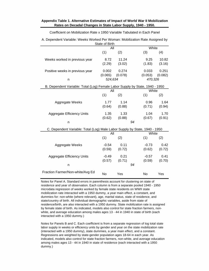
(1) (2) (3) (4)

8.72 11.24 9.25 10.82(2.29) (3.02) (1.83) (3.16)

0.002 0.274 0.033 0.251(0.065) (0.078) (0.053) (0.082)

n

(1) (2) (1) (2)

1.77 1.14 0.96 1.64(0.64) (0.88) (0.71) (0.94)

1.35 1.33 1.04 1.70(0.62) (0.88) (0.67) (0.91)

n

(1) (2) (1) (2)

-0.54 0.11 -0.73 0.42(0.59) (0.72) (0.62) (0.72)

-0.49 0.21 -0.57 0.41(0.57) (0.71) (0.59) (0.70)

n

Appendix Table 1. Alternative Estimates of Impact of World War II Mobilization Rates on Decadal Changes in State Labor Supply, 1940 - 1950.

Coefficient on Mobilization Rate x 1950 Variable Tabulated in Each Panel

Yes

Weeks worked in previous year

Positive weeks in previous year

524,634 470,326

Fraction Farmer/Non-white/Avg Ed No Yes No

94

A. Dependent Variable: Weeks Worked Per Woman: Mobilization Rate Assigned by State of Birth

B. Dependent Variable: Total (Log) Female Labor Supply by State, 1940 - 1950

Aggregate Weeks

Aggregate Efficiency Units

All White

All White

C. Dependent Variable: Total (Log) Male Labor Supply by State, 1940 - 1950

Aggregate Weeks

Aggregate Efficiency Units

94

All White

Notes for Panel A. Standard errors in parenthesis account for clustering on state of residence and year of observation. Each column is from a separate pooled 1940 - 1950 microdata regression of weeks worked by female state residents on WWII state mobilization rate interacted with a 1950 dummy, a year main effect, a constant, and dummies for: non-white (where relevant), age, marital status, state of residence, and state/country of birth. All individual demographic variables, aside from state of residence/birth, are also interacted with a 1950 dummy. State mobilization rate is assigned by female state of birth. As indicated, models also control for state fraction farmers, non-white, and average education among males ages 13 - 44 in 1940 in state of birth (each interacted with a 1950 dummy.)

Notes for Panels B and C. Each coefficient is from a separate regression of log total state labor supply in weeks or efficiency units by gender and year on the state mobilization rate (interacted with a 1950 dummy), state dummies, a year main effect, and a constant. Regressions are weighted by state-gender population ages 18-64 in each year. As indicated, models also control for state fraction farmers, non-white, and average education among males ages 13 - 44 in 1940 in state of residence (each interacted with a 1950 dummy.)

(1) (2) (3) (4)

All 14 - 64 9.06 8.28 9.85 8.73(2.35) (2.39) (2.05) (2.39)

Ages 14 - 17 1.38 1.20 1.41 0.88(0.35) (0.42) (0.32) (0.39)

Ages 18 - 24 2.35 4.85 2.24 5.06(0.94) (1.19) (0.99) (1.32)

Ages 25 - 34 1.26 2.16 0.57 2.00(0.95) (1.55) (0.88) (1.58)

Ages 35 - 44 1.89 2.32 2.41 2.31(0.72) (0.93) (0.73) (0.93)

Ages 45 - 54 1.54 -2.10 2.23 -1.44(1.10) (1.56) (1.05) (1.55)

Ages 55 - 64 0.65 -0.15 1.00 -0.08(0.99) (1.08) (0.96) (1.05)

8th Grade and Below -2.27 -0.79 -1.05 -0.82(1.97) (1.78) (1.47) (1.76)

-2.44 1.93 -2.75 1.75(1.53) (1.56) (1.51) (1.49)

12th Grade and Above 13.78 7.13 13.65 7.81(1.77) (1.79) (1.85) (2.02)

n 585,745 530,026

9th Grade to 11th Grade

YesFraction Farm, Non-white, Avg Ed

No Yes No

A. Weeks Worked by Age Group

B. Weeks Worked by Education Group

Appendix Table 2. Impact of World War II Mobilization Rates on Female Labor Supply by Age and Education: 1940 - 1950.

Dependent Variable: Annual Weeks Worked

Coefficient on Mobilization Rate Variable x 1950

All Females White Females

Standard errors in parenthesis account for clustering on state of residence and year of observation. Each entry is from a separate pooled microdata regression for the relevant demographic subgroup of female weeks worked by state of residence on state mobilization rate interacted with a 1950 dummy, a year main effect, a constant, and dummies for non-white (where relevant), age, marital status, state of residence, and state/country of birth. All individual demographic variables, aside from state of residence/birth, are also interacted with a 1950 dummy. As indicated, models also control for state fraction farmers, non-white, and average education among males ages 13 - 44 in 1940 in women's state of residence (each interacted with a 1950 dummy). Education categories reflect the highest grade completed.

Cohorts

Ages 14 - 24 (1940) 6.11 19.02 4.16 18.14Ages 24 - 34 (1950) (5.24) (5.48) (5.25) (5.71)

n

Ages 25 - 34 (1940) -3.52 16.84 -2.33 16.21Ages 35 - 44 (1950) (4.04) (6.14) (3.55) (6.53)

n

Ages 35 - 44 (1940) 21.16 15.19 23.42 17.76Ages 45 - 54 (1950) (5.39) (7.38) (5.40) (7.23)

n

Ages 45 - 54 (1940) 11.56 -8.19 13.91 -6.45Ages 55 - 64 (1950) (5.82) (5.22) (5.46) (4.75)

n

155,272 138,870

Appendix Table 3. Impact of World War II Mobilization Rates on Female Labor Supply by Cohort: 1940 - 1950.Dependent Variable: Annual Weeks Worked

Coefficient on Mobilization Rate Variable x 1950All White

100,125 92,550

135,893 122,083

115,025 103,918

YesFraction Farm, Non-white, Avg Ed

No Yes No

Standard errors in parenthesis account for clustering on state of residence and year of observation. Each entry is from a separate pooled 1940 - 1950 microdata regression of individual weeks worked by females from the listed cohort on state mobilization rate interacted with a 1950 dummy, a year main effect, a constant, and dummies for: non-white (where relevant), age, marital status, state of residence, and state/country of birth. All individual demographic variables, aside from state of residence/birth, are also interacted with a 1950 dummy. As indicated, models also control for state fraction farmers, non-white, and average education among males ages 13 - 44 in 1940 in female's state of residence (each interacted with a 1950 dummy). Mobilization rate is assigned by female state of residence.

(1) (2) (3) (4) (5) (6) (7) (8) (9) (10) (11) (12)

IV - Weeks Worked per Woman -0.103 -0.068 -0.041 0.018 -0.158 -0.145 -0.061 -0.023 -0.030 0.012 -0.064 -0.032(0.023) (0.041) (0.021) (0.022) (0.035) (0.075) (0.014) (0.019) (0.015) (0.013) (0.020) (0.023)

13.02 9.35 14.70 14.05 11.22 7.21 13.10 9.76 15.34 14.07 11.19 7.65(2.39) (2.70) (4.15) (3.76) (1.96) (3.00) (2.37) (2.67) (4.01) (3.97) (1.93) (2.80)

OLS -Weeks Worked per Woman -0.007 0.007 0.000 0.010 -0.035 0.005 -0.008 0.004 -0.005 0.004 -0.014 0.006(0.010) (0.006) (0.007) (0.006) (0.015) (0.008) (0.006) (0.003) (0.004) (0.003) (0.008) (0.007)

n

(1) (2) (3) (4) (5) (6) (7) (8) (9) (10) (11) (12)

IV - Weeks Worked per Woman -0.108 -0.072 -0.018 0.001 -0.155 -0.135 -0.071 -0.021 -0.024 0.014 -0.063 -0.031(0.025) (0.038) (0.028) (0.022) (0.033) (0.071) (0.015) (0.017) (0.017) (0.013) (0.018) (0.022)

11.68 11.20 11.84 15.05 11.64 8.04 11.65 11.44 11.76 14.46 11.41 8.28(2.14) (2.72) (3.80) (4.03) (1.99) (3.08) (2.16) (2.73) (3.81) (4.08) (1.99) (2.86)

OLS -Weeks Worked per Woman -0.012 -0.001 0.008 0.008 -0.033 0.002 -0.009 0.000 0.001 0.003 -0.016 0.002(0.010) (0.007) (0.008) (0.006) (0.016) (0.007) (0.006) (0.003) (0.005) (0.003) (0.008) (0.006)

n

Fraction Farm/Non-white/Avg Ed No Yes No Yes No Yes No Yes No Yes No Yes

Region x 1950 Dummies No No Yes Yes No No No No Yes Yes No No

Excluding South No No No No Yes Yes No No No No Yes Yes

155,74355,847

78,094 213,966

198,38569,335

Females Males

1st Stage Coefficient(Mobilization Rate x 1950)

1st Stage Coefficient(Mobilization Rate x 1950)

B. Full-Time Weekly Earnings: Whites

58,727 161,683

Appendix Table 4. IV Specifications: Impact of Female Labor Supply on Female and Male Earnings 1940 - 1950:Dropping the South and Adding 4 Region x 1950 Dummies

Dependent Variable: Log Weekly Earnings

A. Full-Time Weekly Earnings: AllFemales Males

Standard errors in parentheses account for clustering on state and year of observation. Samples and specifications are identical to Table 9 columns 3 and 4 (females) and columns 7 and 8 (males) except as noted for addition of 4 Census main geographic dummies (interacted with a 1950 dummy) and dropping of the Southern region in columns 5, 6, 11 and 12 (VA, AL, AR, FL, MS, NC, SC, TX, KY, MD, OK, TN, and WV).

(1) (2) (3) (4) (5) (6) (7) (8)

IV - Weeks Worked per Woman -0.095 -0.078 -0.078 -0.131 -0.068 -0.051 -0.052 -0.029(0.038) (0.030) (0.030) (0.049) (0.022) (0.017) (0.018) (0.018)

Lagged Dependent Variable -0.033 -0.085 -0.084 -0.402 0.025 -0.048 -0.046 -0.062(1940 State Mean Log Wage x 1950) (0.084) (0.063) (0.062) (0.153) (0.073) (0.059) (0.060) (0.071)

9.40 10.24 10.23 8.87 7.82 9.38 9.37 11.85(2.07) (2.59) (2.59) (2.74) (2.08) (2.29) (2.29) (3.19)

n

(1) (2) (3) (4) (5) (6) (7) (8)

IV - Weeks Worked per Woman -0.070 -0.057 -0.057 -0.097 -0.060 -0.047 -0.049 -0.029(0.028) (0.023) (0.024) (0.034) (0.018) (0.015) (0.016) (0.017)

Lagged Dependent Variable -0.284 -0.275 -0.277 -0.360 -0.102 -0.148 -0.143 -0.093(1940 State Mean Log Wage x 1950) (0.074) (0.052) (0.053) (0.113) (0.063) (0.048) (0.051) (0.077)

10.22 11.73 11.71 11.10 8.90 10.78 10.77 12.88(1.64) (2.49) (2.49) (2.60) (1.84) (2.21) (2.21) (3.22)

nFemale Age Structure No Yes Yes Yes No Yes Yes Yes

State of Birth No No Yes Yes No No Yes Yes

Fraction Farm/Non-white/Avg Ed No No No Yes No No No Yes

Appendix Table 5. Lagged Dependent Variable IV Specifications: Impact of Female Labor Supply on Female and Male Earnings 1940 - 1950

Dependent Variable: Log Weekly Earnings

A. Full-Time Weekly Earnings: AllFemales Males

Standard errors in parentheses account for clustering on state and year of observation. Each column is from a separate pooled 1940 - 1950 microdata regression of log weekly earnings on weeks worked per female by state of residence instrumented by state mobilization rate (interacted with 1950 dummy). The lagged dependent variable is equal to the 1940 state mean log weekly full-time wage for the relevant gender/race group interacted with a 1950 dummy. Specifications and control variables are otherwise identical to Table 9.

1st Stage Coefficient(Mobilization Rate x 1950)

78,094 213,966

B. Full-Time Weekly Earnings: WhitesFemales Males

1st Stage Coefficient(Mobilization Rate x 1950)

69,335 198,385

(1) (2) (3) (4) (1) (2) (3) (4)

ln(LSFemale/LSMale) -0.385 -0.579 -0.583 20.1 -0.707 -0.837 -0.845 -1.410(0.089) (0.168) (0.171) (311.8) (0.194) (0.259) (0.267) (1.265)

-0.039 -0.028 -0.014 13.0 0.094 0.138 0.156 -1.733(0.105) (0.122) (0.114) (291.5) (0.171) (0.200) (0.191) (4.184)

2.10 1.77 1.77 -0.03 1.17 1.06 1.06 0.24(0.39) (0.47) (0.47) (0.42) (0.32) (0.35) (0.35) (0.40)

Implied Female Demand σF -2.36 -1.65 -1.68 0.03 -1.63 -1.43 -1.45 -0.32

Implied M/F Substition σM/F -25.48 -36.36 -69.99 n/a n/a n/a n/a -0.58

p-value of H0: (σF)-1 = 0 0.02 0.03 0.03 0.96 0.07 0.10 0.10 0.55

n

Female Age Structure No Yes Yes Yes No Yes Yes Yes

State of Birth No No Yes Yes No No Yes Yes

Farm/Non-white/Avg Ed No No No Yes No No No Yes

Appendix Table 6. IV Estimated Impact of Female Labor Supply on Female/Male Earnings Differential 1940 - 1960

Dependent Variable: Full-Time Log Weekly Earnings

A. All B. Whites

566,221 517,458

ln(LSFemale/LSMale)x Female

1st Stage Coefficient(Mobilization Rate x 1960)

Standard errors in parentheses account for clustering on state and year of observation. Each column is from a separate pooled 1940 and 1960 microdata regression of log weekly male and female earnings on the log ratio of female to male non-farm labor supply in weeks instrumented by the state mobilization rate interacted with a 1960 dummy. Sample definition and specifications are identical to Table 10 columns 1 - 4 except that 1960 Census data is used in place of 1950 Census data.

Figure 1. Labor Force Participation by Gender of U.S. Residents Ages 16 - 65, 1890 - 1990. Source: Blau, Ferber and Winkler (2000), Table 4.1

85.7 85.2 84.682.1 82.5

86.483.3

79.977.4

20.0 21.4 22.7 23.6

33.937.7

43.3

51.5

76.4

84.3

57.5

18.2

27.9

10

20

30

40

50

60

70

80

90

100

1890 1900 1910 1920 1930 1940 1950 1960 1970 1980 1990

Per

cent

Males Females

Figure 2. Male and Female Labor Force Participationand Military Active Service Personnel, 1940 - 1952.

81.5

67.7

84.3 84.684.2

29.0

33.8

30.132.9

8.3

25.4

3.3 2.9

27.8

1.0

0

10

20

30

40

50

60

70

80

90

100

1940 1942 1944 1946 1948 1950 1952

Per

cent

age

poin

ts

0

10

20

30

40

50

60

Per

cent

age

Poi

nts

Male LF/Pop ages 14-64 (left axis) Female LF/Pop ages 14-64 (right axis)

Males % Active Duty ages 14-64 (right axis)

Figure 3. State WWII Mobilization Rates and Female Labor Supply, 1940 - 1960

Coef = 5.23 se = 7.65 t = 0.68

Mobilization Rate and Mean Female Weeks Worked in 1940.4 .45 .5 .55

0

2

4

6

8

10

12

14

16

18

CT

ME

MANHRI

VT

DE NJNY

PA

IL

INMI OHWIIA

KS

MNMO

NE

NDSDVAAL

AR

FLGA

LA

MS

NC SC

TXKY

MD

OK

TN

WV

AZCO

ID

MT

NMUT

WY

CA

ORWA

Coef = 15.41 se = 3.34 t = 4.62

Mobilization Rate and Change in Female W eeks Worked 1940-50.4 .45 .5 .55

-1

0

1

2

3

4

5

6

CT

ME

MA

NH

RI

VT

DE

NJ

NY

PAILINMI

OHWI

IA

KS

MN

MO

NE

ND

SD

VA

AL

AR

FL

GALA

MS

NC

SC

TX

KY

MD

OK

TN

WVAZ

CO

ID

MT

NM

UTWY

CA

ORWA

Coef = -4.75 se = 2.42 t = -1.97

Mobilization Rate and Change in Female W eeks Worked 1950-60.4 .45 .5 .55

-1

0

1

2

3

4

5

6

CTME

MA

NH

RI

VTDE NJ

NYPA

IL

IN

MIOH

WIIA

KS

MN

MO

NE

ND

SD

VA

AL

AR

FLGA

LA

MS

NCSC

TXKYMD

OK

TN

WV

AZ

CO

ID

MT

NMUT

WY

CA

ORWA

A. 1940 Cross section

B. 1940 - 1950 Change

C. 1950 - 1960 Change

Figure 4. State WWII Mobilization Rates and Changes in Male and Female Mean Log Weekly Wages, 1940 - 1950

Mobilization Rate and Log Female W age Change 1940-50

Delta log weekly wages Fitted values

.4 .45 .5 .55

.25

.5

.75

1

1.25

1.5

CTME

MA

NH

RI

VT

DE

NJNYPA

ILINMI

OHWI

IAKS

MNMO NENDSDVA

ALAR

FLGA

LAMS

NC

SC

TX

KY MDOKTN

WV

AZ

CO

ID

MTNM

UTWY

CA

ORWA

A. Females

Mobilization Rate and Log Male Wage Change 1940-50

Delta log weekly wages Fitted values

.4 .45 .5 .55

.25

.5

.75

1

1.25

1.5

CTME

MANH

RI

VTDENJNY

PAILINMI OHWI

IAKS

MN

MO NEND

SD VAALAR FLGA LAMSNC

SC

TXKYMD

OKTN

WV

AZCOID

MT

NM

UTWY

CA

ORWA

B. Males

Figure 5. State WWII Mobilization Rates and Changes in Male and Female Mean Log Weekly Wages, 1940 - 1950

Mobilization Rate and Log Female W age Change 1950-60

Delta log weekly wages Fitted values

.4 .45 .5 .55

.25

.5

.75

1

1.25

1.5

CTME MA

NHRI

VT

DE

NJNY PAIL

INMI

OHWIIA KSMNMO

NENDSD

VAALAR

FL

GALA

MSNC

SC TXKY MD

OKTN

WV

AZCO

IDMT

NM

UTWY CA ORWA

Mobilization Rate and Log Male Wage Change 1950-60

Delta log weekly wages Fitted values

.4 .45 .5 .55

.25

.5

.75

1

1.25

1.5

CT

MEMA

NH RIVTDE NJ

NY PAILINMI OHWIIA KS

MNMO NEND

SD

VAAL

AR

FLGA

LAMS

NC SCTXKY

MD

OKTN WV

AZCO

IDMT

NM UTWY

CA

ORWA

A. Females

B. Males

Figure 6. Estimated Impact of State WWII Mobilization Rate on Standardized Quarters Worked Annually by Women Who Were Ages 16 - 55 in 1945: 1947 - 1977.

-3

-2

-1

0

1

2

3

4

5

1947 1951 1955 1959 1963 1967 1971 1975

Coefficient on Mobilization Measure 90 Percent Confidence Interval