NBER WORKING PAPER SERIES

THE IMPACT OF EARLY OCCUPATIONAL CHOICE ON HEALTH BEHAVIORS

Inas Rashad KellyDhaval M. DaveJody L. SindelarWilliam T. Gallo

Working Paper 16803http://www.nber.org/papers/w16803

NATIONAL BUREAU OF ECONOMIC RESEARCH1050 Massachusetts Avenue

Cambridge, MA 02138February 2011

The authors gratefully acknowledge funding from the National Institute of Aging (R01 AG027045). Maureen Canavan provided excellent research assistance. The views expressed herein are those ofthe authors and do not necessarily reflect the views of the National Bureau of Economic Research.

NBER working papers are circulated for discussion and comment purposes. They have not been peer-reviewed or been subject to the review by the NBER Board of Directors that accompanies officialNBER publications.

© 2011 by Inas Rashad Kelly, Dhaval M. Dave, Jody L. Sindelar, and William T. Gallo. All rightsreserved. Short sections of text, not to exceed two paragraphs, may be quoted without explicit permissionprovided that full credit, including © notice, is given to the source.

The Impact of Early Occupational Choice On Health BehaviorsInas Rashad Kelly, Dhaval M. Dave, Jody L. Sindelar, and William T. GalloNBER Working Paper No. 16803February 2011JEL No. I0

ABSTRACT

Occupational choice is a significant input into individuals’ health investments, operating in a mannerthat can be either health-promoting or health-depreciating. Recent studies have highlighted the potentialimportance of initial occupational choice on subsequent outcomes pertaining to morbidity. This studyis the first to assess the existence and strength of a causal relationship between initial occupationalchoice at labor entry and subsequent health behaviors and habits. We utilize the Panel Study of IncomeDynamics to analyze the effect of first occupation, as identified by industry category and blue collarwork, on subsequent health outcomes relating to body mass index, obesity, alcohol consumption, andphysical activity in 1999-2005. Our findings suggest that initial occupations described as craft, operative,and service are related to higher body mass index and obesity later in life, while labor occupationsare related to higher probabilities of smoking later in life. Blue collar work early in life is associatedwith increased probabilities of obesity and smoking, and decreased physical activity later in life, althougheffects may be masked by unobserved heterogeneity. Few effects are found for the effect of initialoccupation on alcohol consumption. The weight of the evidence bearing from various methodologies,which account for non-random unobserved selection, indicates that at least part of this effect is consistentwith a causal interpretation. These estimates also underscore the potential durable impact of earlylabor market experiences on later health.

Inas Rashad KellyQueens College / CUNYEconomics Department300 Powdermaker Hall65-30 Kissena BoulevardFlushing, NY 11367and NBERInas.Kelly@qc.cuny.edu

Dhaval M. DaveBentley UniversityDepartment of Economics175 Forest Street, AAC 195Waltham, MA 02452-4705and NBERddave@bentley.edu

Jody L. SindelarYale School of Public HealthYale University School of Medicine60 College Street, P.O. Box 208034New Haven, CT 06520-8034and NBERjody.sindelar@yale.edu

William T. GalloCUNY School of Public HealthHunter College / CUNY425 E. 25th Street, Rm. 817 WNew York, NY 10010william.gallo@hunter.cuny.edu

2

I. INTRODUCTION

Working is an activity that occupies much of many individuals’ lives. According to the

2005 American Time Use Survey, employed individuals spend an average of 7.5 hours a day

working. A sizeable economics literature has established that early labor market history,

including occupational choice, influences job mobility and income trajectories (Oreopoulos and

von Wachter 2006; Light 2005). Economic resources have, in turn, been shown to affect health

outcomes (Smith 1999). The presence of a compensating wage differential, wherein individuals

routinely trade off job safety and higher wages, and the presence of substantial heterogeneity in

health care access across occupation and industry classes, further implicate occupational choice

as a significant input into health investments.1

This interplay of various reinforcing and competing mechanisms suggests that work-life

can be both health-promoting and also health-depreciating. Moreover, it may impact health

investments and health outcomes directly, for instance through occupational hazards or job

strain, as well as indirectly, through health care coverage, income, and peer influences. Given

these numerous plausible pathways, a number of studies have examined the association between

job conditions and health (Case and Deaton 2005; Theorell 2000), though most have been

limited by potential selection bias and are unable to draw stronger conclusions regarding

causality. Using the Health and Retirement Survey, Gueorguieva et al. (2009) conduct a more

careful analysis and uncover significant gaps in baseline health by occupation that persist over

time.

Most of the extant literature has also focused on contemporaneous effects rather than the

cumulative durable impact of early labor market choices. This is surprising given that the

1 See Viscusi and Aldy (2003) for a review of the literature on the value of a statistical life derived from the tradeoff between wages and job safety.

3

economic paradigm, which views health as a capital stock determined by lifetime investments,

choices, and constraints (Grossman 1972), imparts a significant role to early investments and

resources. Furthermore, the impact of economic resources and other choices may be most acute

during childhood or early adulthood, when health levels and pathways are being established.

The importance of a lifetime budget constraint implies that additional economic resources may

not have a quantitatively large impact on the current health capital stock, especially as the

individual gets older (Smith 1999). Even if health behaviors or health utilization respond to

current changes in circumstances, effects on health capital may not be realized until later in the

working life-course, suggesting that the cumulative or durable impact of labor market choices

may be more salient than contemporaneous effects.

A budding literature and, in particular, three seminal studies (Fletcher and Sindelar 2009;

Fletcher et al. 2009; Sindelar et al. 2007) have recently pointed to potentially important effects of

initial occupational choice on subsequent health status, with substantial heterogeneity across

socio-demographic groups. These analyses, however, have been limited to self-rated health and

the incidence of heart attacks. The reduced-form approach in these studies also obfuscates

potential pathways and interim effects on health inputs. We attempt to address these gaps, and in

the process make significant contributions to the emerging focus on the importance of early

occupational choice for subsequent health, and to the broader economics literature on the lasting

effects of early circumstances on health and labor outcomes.

This study is the first to assess the existence and strength of a causal relationship between

initial occupational choice at labor entry and subsequent health behaviors and habits, such as

smoking, drinking, physical activity, and body mass index, all of which are important proximate

inputs into later health status. Health habits are often established relatively early in life (Fletcher

4

and Sindelar 2009) and therefore more likely to respond to early labor market choices. The

focus on health behaviors also underscores potential pathways through which initial labor market

choices may eventually have lasting effects on health; the identified impact of initial occupation

on later health outcomes (for instance, heart attacks, as studied in Sindelar et al. 2007) is more

plausibly indicative of a causal link if effects on intermediate health behaviors and inputs are

also evident. We also undertake an exploratory analysis of potential mediators and pathways,

including income trajectories, health insurance, work hours, and other factors, through which

early occupational choice may have durable effects on subsequent health habits. Identifying

these pathways can be important in targeting public policy interventions that may moderate

potentially adverse effects on health behaviors and overall health status.

The empirical analysis is based on the Panel Study of Income Dynamics (PSID), a

nationally-representative longitudinal data set that contains information on over 65,000

individuals spanning as much as 36 years of their lives. The PSID contains extensive

information on pre-labor market conditions and family characteristics, as well as typically-

unobserved measures such as individuals’ risk tolerance, which allows us to account for potential

selection bias. We further employ a series of methodologies to disentangle causal effects,

including a standard instrumental variables-based strategy; an innovative approach proposed by

Altonji et al. (2005) that permits causal inference without the need for exclusion restrictions or

other strong restrictive assumptions; and a novel approach proposed by Lewbel (2007) that

generates internal instrumental variables in the presence of heteroscedastity. This direct focus on

accounting for selection bias and sorting out causality is another contribution that we make over

much of the literature. Understanding the interplay over the life-course among early labor

5

market choices and health investments is important to the development of effective policies and

programs to improve health at older ages.

The remainder of the paper proceeds as follows. Section II discusses potential

mechanisms through which initial occupational choice may influence health behaviors, and also

places our study within the context of the extant literature. Section III describes our empirical

strategies for accounting for potential selection bias, followed by a description of the data

sources in Section IV. Section V presents and discusses the estimates from our multivariate

analyses. Section VI concludes with some implications for public policy.

II. ANALYTICAL FRAMEWORK

The objective of this study is to assess the extent to which first occupation impacts

subsequent health behaviors among older adults. This question can be framed within the human

capital model for the demand for health (Grossman 1972). Grossman combines the household

production model of consumer behavior with the theory of human capital investment to analyze

an individual’s demand for health capital. Individuals invest in health up to the point where the

marginal benefit equates the supply price of health capital at each age. The basic insight of this

paradigm is that health is a capital stock and health behaviors and other inputs are investments in

that stock. For a rational utility maximizing agent with a lifetime horizon, today’s health stock

will be a function of the entire history of health investments including current and past health

behaviors, incomes, and health endowments.

Occupational choice, in general, is expected to be an input into health production and

affect health outcomes and behaviors through a variety of channels. Aspects of work can have

both direct and indirect effects on health, which may be health-promoting or health-depreciating.

Direct effects include occupational exposure to health and safety hazards, job strain and stress

6

related to working conditions, and injury risks. Often a compensating wage differential is

present wherein the individual is trading off job safety for higher wages, particularly in unskilled

jobs. Thus, occupational choice is also a form of direct investment in health.2 The Occupational

Safety and Health Administration (OSHA) reports 4.1 non-fatal workplace injuries and illnesses

among 100 equivalent full-time workers in 2008.3 This national all-industry average masks

considerable heterogeneity; the rate is much higher among larger firms and among state and local

government employers. Certain private industries such as crop and animal production,

food/beverage and tobacco manufacturing, wood and primary metal manufacturing, hospitals,

and nursing and residential care facilities also exhibit far higher rates of occupational illness and

injury.

Job strain associated with working conditions may also have direct adverse effects on

mental and physical health. In a comprehensive review of the literature on job stress, Michie and

Williams (2003) find that long hours worked, work overload and pressure, and the effects of

these conditions on personal lives are key factors associated with psychological ill health and

sickness absence. Depression and mental illness, in turn, have been found to causally impact

participation in unhealthy behaviors such as smoking, drinking, and illicit drug use (Saffer and

Dave 2005).

Indirect effects of occupational choice on health can occur via shifts in income and

wealth constraints, health insurance coverage, shifts in time constraints, and influences through

workplace peers. For instance, initial occupational choices affect occupational mobility, tenure

and experience, and income trajectories over one’s lifetime (Light 2005); these shifts in

2 See Cropper (1977) for a formal introduction of occupational choice in Grossman’s human capital framework for the demand for health capital. 3 Industry-specific non-fatal workplace injury and illness rates are available at: http://www.bls.gov/iif/oshsum.htm.

7

economic resources would in turn be expected to impact health. While the direction of causality

is not well-established, a sizeable literature documents a strong association between income or

wealth and a variety of health outcomes including mortality and morbidity (Smith 1999). Ettner

(1996), in an attempt to disentangle causality, applies an instrumental variables-based

methodology to three large-scale nationally representative data sets. She estimates the structural

impact of income on health and concludes that increases in income significantly improve mental

and physical health, but also increase the prevalence of alcohol consumption.

The prevalence of uninsured individuals also varies substantially across occupation and

industry classes, which in turn may mediate the impact of occupational choice on health. For

instance, among non-professional and non-managerial occupations, almost half of all non-elderly

workers in agriculture are uninsured, 40% of such workers in construction are uninsured, and

25% of workers in the wholesale and retail trade lack insurance.4 Summarizing the results from

the Rand Health Insurance Experiment, Newhouse (2004) concluded that higher coinsurance

rates and lack of access to care reduced health care utilization, and while for “most people

enrolled in the RAND experiment, who were typical of Americans covered by employment-

based insurance, the variation in use across the plans appeared to have minimal to no effects on

health status … for those who were both poor and sick – people who might be found among

those covered by Medicaid or lacking insurance – the reduction in use was harmful, on average.”

McWilliams et al. (2007) similarly find that compared with previously insured adults, previously

uninsured adults reported significantly improved health trends after becoming eligible for

Medicare at age 65. Numerous studies have also shown that physician advice and interventions

are successful in influencing patient behaviors such as smoking, drinking, exercise, and diet

4 See Health Insurance Coverage in America, 2008, accessed at The Kaiser Family Foundation website: http://facts.kff.org/chartbook.aspx?cb=57.

8

(Dave and Kaestner 2009; U.S. Preventive Services Task Force 2004, 2003). Subsequently, lack

of access to primary care due to interruptions in health insurance may lead to unhealthy

lifestyles. Hadley (2003), in a review of the literature, likewise concludes that, while all studies

have methodological issues, research over the past 25 years makes a compelling case that having

health insurance and greater health care utilization would improve the health of the uninsured.

Data from the American Time Use Surveys (ATUS) indicate that work-related physical

activity (measured in equivalent metabolic units) varies substantially across occupations, being

expectedly largest in mining, agriculture, construction, and manufacturing jobs, and lowest

among management and administrative jobs. Leisure-time physical activity also varies across

occupations, often in inverse relation to work-related activity, suggesting some substitution

between the two types driven by time constraints. This heterogeneity in physical activity across

jobs, combined with differential effects of work-related versus leisure-time physical activity,

would be expected to impact body mass index and subsequent health status, ceteris paribus.

As much of life is spent working, social influences through workplace peers may also

impact individuals’ health behaviors. Moon and Kim (2001), for instance, estimate prevalence

of cigarette smoking by occupation and industry in the U.S., using data from the National Health

and Nutrition Examination Survey. They document considerable differences across occupations

and industries. Smoking prevalence is highest among material movers, construction laborers,

and vehicle mechanics and repairers, and lowest among teachers. Among industry groups, the

construction industry had the highest prevalence of cigarette smoking. Powell et al. (2005)

conclude that peer effects have a significant impact on youth smoking behavior and that there is

a strong potential for social multiplier effects. Thus, with respect to initial occupation, health

9

behaviors of young adults and youth may be especially susceptible to peer influences at the

workplace.

Prior Studies

Given these plausible mechanisms, numerous social scientists have studied the empirical

relationship between work status, job characteristics, and health.5 For instance, the longitudinal

Whitehall studies examine the health of civil servants in London, focusing on how occupation

affects health (Marmot and Smith 1997; Marmot and Bobak 2000; Marmot 2001). In general,

these studies find that occupational status, job insecurity, and stress, among other factors, impact

various dimensions of health, including coronary heart disease, self-reported health status,

various morbidities, and health behaviors.

This literature, however, has largely ignored any potential durable impact of occupational

choice. Three recent studies address this gap and acknowledge the importance of early

occupational choice; these studies are the first to empirically investigate how initial occupation

and job characteristics may have a cumulative impact on subsequent health status. Fletcher et al.

(2009) match job characteristics from the Dictionary of Occupational Titles to individual records

from the Panel Study of Income Dynamics (PSID) to investigate the cumulative impact of job

characteristics on self-rated health status. They construct five-year cumulative measures of job

characteristics, and find that individuals working in jobs with high physical demands or harsh

conditions experience declines in their health, with stronger adverse effects for females and older

workers. This is consistent with Fletcher and Sindelar (2009) who also find that a blue-collar

occupation at labor force entry is associated with subsequent decrements in self-reported health

status. Sindelar et al. (2007) aggregate three-digit occupational codes into ten broad categories

and consider the effects of early occupation choice on self-rated health status and ever having a 5 See Theorell (2000) for a review of this literature.

10

heart attack. They also confirm that first-occupation has a durable impact on later health, though

the impact varies by health measure and the degree of control for other observables.

Contributions

Our study adds to this emerging literature on the importance of early occupational choice

on subsequent health and fits within the broader economics literature on lasting effects of early

circumstances on health and labor outcomes. The studies noted above make a seminal

contribution to this literature, though the focus thus far has been on self-rated health status and

on the incidence of heart attacks. This study investigates the impact of first occupation on a host

of subsequent health behaviors including smoking, drinking, physical activity, and body mass

index, all of which are important proximate inputs into health. The focus on health behaviors is

warranted for at least two reasons. First, durable effects on health behaviors (that is, investments

in health) may be relatively more apparent and easier to identify statistically in a consistent

manner than effects on indicators of the health stock. Second, the focus on health behaviors also

underscores potential pathways through which initial labor market choices may eventually have

lasting effects on health. We also undertake a first step in directly investigating channels of

effect, including shifts in income, hours worked, and other potential mediators through which

initial occupational choice may influence health behaviors. Earlier studies have generally

implemented a reduced-form approach, which does not inform the “black box” that links early

occupation to subsequent health. Uncovering evidence of plausible mechanisms also adds to the

weight of the evidence bearing on whether the link represents a causal effect.

Furthermore, since occupational choice may be sticky over one’s lifetime, the durable

effect of first occupation is often confounded with the contemporaneous effect of current

occupation in the prior studies. We are careful to distinguish between these two effects. We also

11

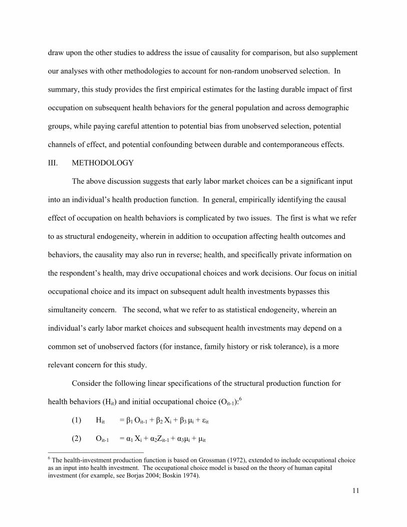
draw upon the other studies to address the issue of causality for comparison, but also supplement

our analyses with other methodologies to account for non-random unobserved selection. In

summary, this study provides the first empirical estimates for the lasting durable impact of first

occupation on subsequent health behaviors for the general population and across demographic

groups, while paying careful attention to potential bias from unobserved selection, potential

channels of effect, and potential confounding between durable and contemporaneous effects.

III. METHODOLOGY

The above discussion suggests that early labor market choices can be a significant input

into an individual’s health production function. In general, empirically identifying the causal

effect of occupation on health behaviors is complicated by two issues. The first is what we refer

to as structural endogeneity, wherein in addition to occupation affecting health outcomes and

behaviors, the causality may also run in reverse; health, and specifically private information on

the respondent’s health, may drive occupational choices and work decisions. Our focus on initial

occupational choice and its impact on subsequent adult health investments bypasses this

simultaneity concern. The second, what we refer to as statistical endogeneity, wherein an

individual’s early labor market choices and subsequent health investments may depend on a

common set of unobserved factors (for instance, family history or risk tolerance), is a more

relevant concern for this study.

Consider the following linear specifications of the structural production function for

health behaviors (Hit) and initial occupational choice (Oit-1):6

(1) Hit = β1 Oit-1 + β2 Xi + β3 μi + εit

(2) Oit-1 = α1 Xi + α2Zit-1 + α3μi + μit

6 The health-investment production function is based on Grossman (1972), extended to include occupational choice as an input into health investment. The occupational choice model is based on the theory of human capital investment (for example, see Borjas 2004; Boskin 1974).

12

Equation (1) is a production function for health behaviors (Hit) at adulthood, which is a function

of occupational choice at labor market entry (Oit-1), observable characteristics such as age,

gender, race, and education (Xi), and unobservable characteristics pertaining to the individual,

such as family background, tolerance towards risk, and the rate of time preference (μi). Equation

(2) postulates the determinants of occupational choice at labor market entry. The vector Zit-1

represents observed and unobserved variables specific to the occupation decision, such as

parental occupation, initial labor market conditions, or private information regarding expected

costs and benefits associated with the occupational choice, which may not directly impact the

individual’s subsequent health status (conditional on own and parental income or wealth, and

other investments). The vector μi denotes common unobserved determinants of occupational

choice that may also influence health. The subscripts refer to the ith individual in time period t,

and t-1 denotes initial labor market entry or earlier periods.

Our objective is to estimate β1 in order to assess the existence and strength of a possible

causal relationship between first occupation and health behaviors. However, single equation

methods applied to equation (1) may not yield causal information due to the presence of non-

random selection into different occupations and investments in health – that is, correlation

between μi and Oit-1 (α3 ≠ 0). Our estimation strategy proceeds in a stepwise fashion. Initially,

we ignore the statistical endogeneity and estimate equation (1) using a standard regression

model. We begin with a parsimonious set of covariates, and then estimate models with an

expanded set of covariates including state fixed effects, family history, risk tolerance, and

employment information, some of which are typically unobserved in other data sets. Estimating

both the basic and the extended models allows us to evaluate how much of the association

between early occupational choice and later health behaviors appears to be driven by omitted

13

individual heterogeneity. If the magnitude of the marginal effect of first occupation is highly

sensitive to the inclusion of the additional covariates and typically-unobserved factors, then it is

likely that factors that remain unobserved also play some role in this relationship.7 This

assumption is reasonable if one is using a multi-purpose, secondary data set, where the

information collected on respondents may not include all information relevant to the outcome

under study (Altonji et al. 2005). In cross-sectional data, which generally would not contain

information on pre-labor entry characteristics and family history, unobserved factors are likely to

be rather influential, whereas this may not be the case in a rich longitudinal data set such as the

PSID, which includes measures of parental investments and family history as well as measures

of the respondent’s tolerance towards risk.

We refer to this problem as selection on observables and selection on unobservables

(Altonji et al. 2005). We use these terms to acknowledge that respondents are not randomly

sorted into occupations and health. Selection on observables refers to observed factors (such as

age, gender, and race) that are correlated with both initial occupation and subsequent health

behaviors. Selection on unobservables refers to possible factors that are not available in our data

set, and will therefore influence the marginal effect of initial occupation.

The degree of selection on the observables can be gauged by comparing the estimated

coefficients on first occupation from the parsimonious and extended models. The degree of

selection on the unobserved characteristics cannot be measured directly with non-experimental

data. However, we can bound this latter effect, allowing us to draw inferences regarding the

unbiased relationship between first occupation and later health behaviors.

7 The direction and magnitude, however, is unknown, depending on the nature of the joint distribution of the observed and unobserved characteristics.

14

Thus, the next step in our empirical strategy relies on an innovative approach proposed

by Altonji et al. (2005), comprising two parts. The first step involves obtaining estimates of the

effect of first occupation on health behaviors from a bivariate probit regression model in which

the correlation between unobserved variables is fixed at various levels. This part of the analysis

allows us to assess how sensitive estimates of the effect of first occupation are to the potential

problem of correlated unobservables. The second step computes the amount of sorting into first

occupation and adult health behaviors on observed variables, and obtains estimates of the effect

of first occupation under the assumption that the degree of sorting on unobserved variables is

equal to the degree of sorting on observed variables.

Specifically, alternately defining healthy behaviors and first occupation as dichotomous

indicators (described below), application of the bivariate probit model assumes that εi and μi are

distributed bivariate normally with a correlation of ρ and unit variances.8 First, we estimate a

bivariate probit model without any identifying assumptions but with a constrained correlation

coefficient, ρ. We constrain ρ to be 0.10 initially and then examine the effects of increasing ρ in

increments of 0.10 to 0.20, 0.30, 0.40 and 0.50. Since it is also plausible that unobserved factors

common to both blue collar work and health behaviors are negatively correlated, we then

constrain ρ to be -0.10, increasing incrementally (in absolute value) to -0.20, then -0.30, -0.40,

and -0.50. In this way, we impose on the model increasingly greater amounts of correlation

between unobservables, and examine whether or not the effect of first occupation on health

behaviors is robust to such changes. This analysis allows one to determine the threshold of

selection on unobservables, if any, at which first occupation no longer has a statistically

significant effect on health behaviors.

8 The model is estimated using maximum likelihood (Evans and Schwab 1995; Goldman et al. 2001).

15

Altonji et al. (2005) argue that if the observable determinants of an outcome are truly just

a random subset of the complete set of determinants, selection on observable characteristics must

be equal to selection on unobservable characteristics. This assertion of equal selection is unlikely

to be true, and in fact, given our specialized longitudinal data set, we would expect selection on

observable factors to be greater than selection on unobservable factors. Thus, estimates obtained

under the assumption of equal selection are likely biased downwards, and represent a lower-

bound estimate. The upper bound effect is the estimate from the naïve single equation extended

model that assumes no additional selection on unobservable variables.

The advantage of the Altonji et al. (2005) procedure is that it allows researchers to assess

the possible existence and strength of a causal relationship without requiring the use of

identifying assumptions that are often not credible – for example, the existence of valid

instruments in an instrumental variables context or other ad hoc exclusion restrictions. As a

result, without any other identifying assumptions, researchers can estimate the degree of sorting

on unobservable factors using the observed data, and identify a lower bound on the causal

parameter estimate.

We also supplement our analyses with additional robustness checks in order to add to the

weight of the evidence on the issue of causality. While instrumental variables-based

methodologies are difficult to implement in practice, owing to the challenges in identifying

plausible exclusion restrictions, we follow Fletcher and Sindelar (2009) in using parental

occupation (conditional on parental income and education) and early state labor market

conditions as instrumental variables (IV) for first occupational choice. Diagnostic tests are

consistent with the identifying assumption that these measures have no direct impact on future

health behaviors (outside of their impact through occupational choice), and that these measures

16

are significant predictors of first occupation. These estimates should, nevertheless, be interpreted

with caution. This part of the analysis does, however, allow us to place our findings on health

behaviors within the context of the sparse, but important, prior studies that have considered

health outcomes. If these prior estimates on health outcomes are plausibly causal, then we should

also see commensurate effects on health behaviors, which are proximate inputs into later health.

This analysis further allows us to compare our lower and upper bound estimates derived under

minimal identifying restrictions with those derived under a more standard IV approach.

Lewbel (2007) presents an IV technique that is useful when valid external instruments are

weak or not available. This procedure relies on the presence of heteroscedasticity in the error

term of the first-stage equation, which is tested using a Breusch-Pagan (1979) test. The Lewbel

IV procedure uses as the identifying instruments, where X is a vector of

independent variables that may include all independent variables or a subset of them, and is

the predicted residual from the first-stage (occupational choice) regression. Therefore, we also

implement an instrumental variables analysis where we exploit the heteroscedastic nature of the

residuals to generate internal instruments. As validation for this technique, we consistently find

evidence of heteroscedasticity in our samples.

As a final step, we implement an exploratory analysis of potential mediators to inform the

strength of the specific mechanisms underlying the impact of first occupation on later health

behaviors. The estimated specifications thus far only include exogenous socioeconomic and

predetermined factors so as not to “over-control” for factors that may be potential pathways. In

alternate analyses, we re-estimate specification (1) by incorporating household income, hours

worked, and current occupational status to gauge the extent to which the estimated effect (if any)

of first occupation on subsequent health behaviors can be explained by these mediators.

17

IV. DATA

The Panel Study of Income Dynamics was begun in 1968 and covers a representative

sample of U.S. individuals (men, women, and children) and the family units in which they reside.

By the end of the 2003 survey, the PSID had collected information from over 65,000 individuals

spanning as much as 36 years of their lives. Starting in 1997, the surveys were conducted

biennially. Between 1968 and 1972, data collection took place through in-person interviews

using paper and pencil questionnaires. Thereafter, most interviews were telephone interviews or,

starting in 1993, computer assisted telephone interviews.9 Comprehensive information on health

behaviors, labor market characteristics, and demographic characteristics are readily available in

the PSID. In our analysis, we use years 1999-2005, yet we exploit the longitudinal nature of the

data set by thoroughly utilizing information from prior years, particularly regarding labor market

characteristics. Information on the head of the household and spouse are used due to the sparse

information on health behaviors for other family members.

Health Outcomes

Body Mass Index: Self-reported weight and height are available in the PSID in the 1986, and

1999-2005 waves, for the head of the household and the wife. The body mass index, or BMI, is

calculated as weight in kilograms divided by height in squared meters. Other measures of

adiposity have been shown to be superior to BMI (Burkhauser and Cawley 2008; Wada and

Tekin 2010). However, they tend to be costly and are not routinely measured in physical

examinations. BMI is a nationally representative figure that provides a reliable approximation of

weight changes over time. Results are not sensitive to applying an adjustment procedure to

correct for potential under-reporting of BMI based on observable characteristics, as employed in

Chou, Grossman and Saffer (2004). 9 Source: http://psidonline.isr.umich.edu/Guide/Overview.html.

18

Obesity: Obesity is defined by the National Institutes of Health as having a BMI of 30 kg/m2 or

greater. According to data from the National Institutes of Health, the percentage of individuals

18 years of age or older classified as obese has risen in the United States from 12.7% in the

1960s to 31.7% in 2004. Obesity carries many risks for a host of disorders, including heart

disease, hypertension, stroke, cancer, and depression (Must et al. 1999; Mokdad et al. 2003). A

variety of economic causes have been explored, including reductions in job strenuousness

(Philipson 2001; Lakdawalla and Philipson 2009), technological innovation in food processing

and preparation (Cutler, Glaeser, and Shapiro 2003), the growing availability of restaurants and

the increased labor force participation of females (Chou, Grossman, and Saffer 2004; Rashad,

Grossman, and Chou 2006), urban sprawl (Ewing et al. 2003), and time preference for the

present (Komlos, Smith, and Bogin 2004; Smith, Bogin, and Bishai 2005; Zhang and Rashad

2008).

Alcohol Consumption: For 1999-2005, the PSID asks the head of the household and their spouse

(if any) to report on the average number of drinks consumed per day. The responses are

categorical (less than one a day; 1-2 drinks; 2-4 drinks; or 5 or more drinks a day), which we

convert to the midpoints of each category (Powers and Xie 2008); we convert the “less than one

a day” category into 0.5 drinks and the “five or more a day” category to 5.5 drinks. Alcohol

consumption – and particularly abuse – can have adverse effects on labor market productivity,

morbidity, mortality, and economic growth (Cesur 2009). Yet some studies have shown that

moderate drinking has a positive effect on wages, largely operating through social networking

channels (Berger and Leigh 1988; French and Zarkin 1995; Hamilton and Hamilton 1997;

McDonald and Shields 2001; Tekin 2004; Bray 2005). Other studies conclude that the positive

19

relationship between moderate drinking and earnings mostly represents unobserved selection

bias (Saffer and Dave 2005; Dave and Kaestner 2002).

Smoking: The PSID asks questions on smoking by the head of the household and the spouse in

1986, and again in the years 1999-2005. We construct a dichotomous indicator for current

smoking as the outcome measure. According to the Centers for Disease Control and Prevention,

tobacco use, which can lead to lung, larynx, esophageal, and oral cancers, is the nation's most

preventable cause of disease, disability, and death.10

Physical Activity: In 1999-2005, the PSID asks heads of households and their spouses to report

on the frequency of light and heavy physical activity. The questions are: “How often do you

participate in light physical activity – such as walking, dancing, gardening, golfing, bowling,

etc.?” and “How often do you participate in vigorous physical activity or sports – such as heavy

housework, aerobics, running, swimming, or bicycling?” Individuals report on their frequency

of participation and a reference time unit, which we standardize to an average weekly frequency.

Physical activity has been shown to be an important factor in keeping morbidity and mortality at

bay, and most Americans do not engage in sufficient amounts of physical activity (USDHHS

1996; Pratt et al. 1999).

First-Occupation Variables

In order to accurately capture information on first occupation, we defined two alternative

measures pertaining to first occupation. The first is based on recall and is asked in 1997-2005:

“Thinking of your first full-time regular job, what kind of work did you do?” Three-digit

occupation codes from the 1970 Census of Population are provided. From these we derived 16

occupational categories: Craft, Operative, Transport, Labor, Farmer, Manager, Sales, Clerical,

Craft, Operative, Transport, Labor, Farmer, Service, Private, and Professional. A dichotomous 10 See http://www.cdc.gov/tobacco/ for more information.

20

variable is further defined as equal to 1 if the category is one of Craft, Operative, Transport,

Labor, or Farmer, and 0 otherwise, denoted as “blue-collar” occupation. We use the most recent

recall (1997) prior to 1999, as well as recalls from the 2003 and 2005 surveys, which use

occupational codes based on the 2000 Census.

The second measure is based on the first occupation reported by the individual in the

PSID, starting from 1968. This measure, by using reported information at the time of first

occupation, minimizes potential recall bias. Since only one-digit occupation codes were initially

coded, we created the following 8 occupational categories based on these one-digit codes: Craft,

Operative, Labor, Farmer, Manager, Self-Business, Clerical, and Professional. A dichotomous

indicator representing blue-collar work is further defined to reflect the following occupations:

Craft, Operative, Labor, or Farmer. Models also control for years since first occupation, defined

as the difference between the current survey year and the year of first-reported occupation, to

capture the effect of time duration since initial labor-market entry.

Individual Characteristics

All models control for individual characteristics pertaining to gender, race/ethnicity,

education, age, marital status, and employment status.11 Alternate models also control for

parental characteristics including the educational status of the mother and father and whether the

family was poor.12

A module probing the individual’s tolerance towards risk is administered to a subset of

individuals in 1996. Measures of risk aversion are obtained from a series of questions involving

11 In our initial specifications, we do not control for mediating factors such as household income and hours worked, which may represent mechanisms through which initial occupation affects health behaviors. Models reported in Table 11 assess the importance of these mediators. 12 Parental education is categorical: (1) grades 0-5, (2) grades 6-8, (3) grades 9-11, (4) grade 12, (5) 12 grades + non-academic training; R.N., (6) some college, no degree; associate’s degree, (7) college baccalaureate degree and no advanced degree mentioned; normal school; RN with 3 years of college, and (8) college, advanced or professional degree; some graduate work.

21

the willingness to choose different levels of lifetime income with varying probabilities. The

module has undergone considerable testing in order to minimize misunderstandings and

additional complications in interpretation, and to ensure consistency with the economist’s

concept of risk preference. Barsky et al. (1997) provide a detailed analysis of the survey

instrument. Answers to the questionnaire separate the individuals into four distinct categories of

risk preference, ranging from the most risk tolerant to the most risk averse.13 Almost half

(48.6%) of the respondents can be classified in the most risk-averse category, with 31.8 percent

divided equally among the second and third most risk-averse groups , and 19.6 percent

comprising the least risk-averse categories. Barsky et al. (1997) validate such a module of risk

tolerance from the Health and Retirement study, and show that it is related to behaviors

(insurance, portfolio allocation, migration, risky health behaviors, self-employment) that would

be expected to vary with an individual’s propensity to take risks. Since the PSID respondents

only partake in the risk module once, the measure of risk tolerance is time-invariant. This is not,

however, a concern, since studies have shown that personality traits associated with risk

tolerance are generally stable, have a biogenic basis, and have some constancy across various

situations (Howard et al., 1997; Menza et al., 1991). Individuals’ propensity for risk-taking is

typically unobserved in other datasets, and represents an important source of non-random

selection into outcomes, since it may affect both occupational choice as well as participation in

other risky and unhealthy behaviors. We include measures of risk-tolerance in supplemental

analyses and extended models to address this potential selection bias.

Instrumental Variables

13 The categories can be ranked in order, without any functional form restrictions on the preference parameters or the utility function.

22

In the instrumental variables (IV) models based on external instruments, we use

information on the county unemployment rate in 1968 (the earliest year county unemployment is

reported) when the average respondent is 18 years of age, and whether the respondent’s father

worked in a blue-collar occupation. Similar instruments (early labor market conditions and

parental occupation) were also utilized by Fletcher and Sindelar (2009). We confirm that these

measures are significant predictors of whether the respondent’s first occupation was blue-collar

in the expected direction. Higher county unemployment rates in the initial wave raise the

probability of blue-collar work; similarly, a respondent is also more likely to work in a blue-

collar occupation if their father did so as well. Conditional on parental education and family

resources, these variables do not have any direct effects on health behaviors as evidenced by the

test of overidentification restrictions. Alternately, these instrumental variables are also

insignificant with close-to-zero magnitudes when included in the extended specifications, again

suggesting that they do not directly impact health behaviors. However, the instruments lack

statistical power and the estimates should therefore be interpreted with caution. This underscores

the difficulties of implementing a conventional IV-based strategy, particularly when analyzing

the effects of early circumstances, since first occupation (at least 30 years prior to current adult

outcomes) is difficult to predict with strong statistical power and in a way that is uncorrelated

with subsequent inputs into health. Thus, alternate approaches with a series of checks add to the

weight of the evidence bearing upon the research question.

Out of approximately 11,000 individuals who were either head of household or spouse in

years 1999-2005, sample sizes after deleting missing information on the aforementioned

variables are: 6971 (year 1999) and 6303 (year 2005). Summary statistics are provided in Table

1.

23

V. RESULTS

Baseline Estimates

Table 1 indicates that the largest fraction of workers first commence their labor market

experience in the Clerical occupational category (approximately 22%), followed by Professional

occupations (~17%). Approximately 36% of respondents were initially blue collar workers

based on recall in 1999 or 2005, and approximately 38% were initially blue collar workers based

on their first reported occupation in the earliest PSID wave. There are significant differences in

health behaviors between individuals whose initial labor market entry was in blue-collar

occupations relative to non-blue collar occupations. In general, initial blue-collar workers tend

to engage in more unhealthy behaviors; they have a higher BMI and are more likely to be obese,

have higher daily alcohol consumption, and are more likely to be current smokers. However,

initial blue-collar workers are also more physically active. These differences are persistent in

both 1999 and 2005.

While these differences in health behaviors are suggestive, individuals are not randomly

selected into initial blue-collar occupations. There are also significant differences with respect to

other observable characteristics between blue-collar and non-blue collar workers. For instance,

initial blue-collar workers are more likely to be male, low-educated, slightly older, married, and

have low-educated and poor parents. Thus, the association between first occupation and

subsequent unhealthy behaviors also reflects confounding due to such non-random selection on

observables and potential selection on unobservables. The multivariate analyses address these

concerns.

Tables 2a and 2b present estimates of the impact of first occupation on BMI in 1999 and

2005, respectively. Estimates are generally robust across the alternate measures of first

24

occupation, whether based on recall in 1999/2005 or generated based on the respondent’s first

reported occupation in the earliest wave. In the limited specification (model 1), when broken

down by occupational category, the Craft, Operative, Transport, Labor, Farmer, Sales, Clerical,

Service, and Private occupations are significantly and positively associated with BMI (0.5 – 1.9

points higher), relative to initial Professional occupation. Aggregating occupations in

specifications 3 and 6 suggests that initial blue-collar work is associated with a 0.4 to 0.7 point

increase in BMI.14 The extended specifications control for state indicators, which capture all

time-invariant state-specific factors, maternal and paternal education, parental poverty status, and

indicators of risk tolerance – measures which are typically unobserved in other datasets.15 The

magnitude of the impact of initial blue-collar occupation is fairly robust to these additional

controls, suggesting a 0.1 – 0.6 point increase in BMI in 1999; the precision of these estimates is

reduced in the extended models due to reduced sample size. This compares to a 1.4 point

increase in BMI, among blue-collar workers, based on the unadjusted means reported in Table 1.

About 50 to 60% of this unadjusted difference is driven by observable factors such as age, race,

education, marital status, and gender. The robustness in the magnitude of the effect between the

limited and extended models suggests that once the basic observables are taken into account,

additional section on other factors may not be significant.

Models 5 and 8 control for prior BMI, as measured from the 1986 PSID wave. Prior

BMI is a strong determinant of current BMI, consistent with the substantial persistence in BMI

over time. The effect of initial blue-collar occupation on 1999 BMI decreases in magnitude and

14 The effects of the other covariates are consistent with the literature on obesity; BMI is higher among individuals who are black (relative to all other races), low-educated, and never-married, and individuals whose parents are low-educated. The BMI-age profile is concave, generally increasing up to ages 50-55 and then declining due to a loss in muscle mass. 15 The coefficients on the indicators of risk tolerance (least risk-averse being the reference category) suggest that more risk-averse individuals have lower BMI.

25

becomes insignificant. This is consistent with initial occupation having a lasting, but

diminishing, effect on health behaviors over time.

The effects of first occupation on BMI in 2005, approximately 26 years on average after

initial labor market entry, are generally consistent with the effects in 1999 noted above. Initial

blue-collar occupation is associated with between a 0.3 to 1.0 point increase in BMI in 2005.

Effect magnitudes are robust across the limited and extended specifications, and diminished

when models control for prior BMI.

Tables 3a and 3b present models for obesity. Consistent with the estimates for BMI,

initial blue-collar occupation is associated with a 3.4 to 6.7 percentage points increase in the

probability of being obese in 1999. The unadjusted difference in means between blue-collar and

non-blue collar workers was about 6 percentage points, again suggesting that as much as 50% of

the observed difference is due to confounding. However, additional control for parental history,

risk tolerance, and state fixed effects do not further diminish the impact of first-occupation.

Results for 2005 show similar patterns with somewhat higher effect magnitudes; initial blue-

collar work is associated with a 4.8 to 9.4 percentage points increase in obesity prevalence.

Note, however, that obesity prevalence was in general higher in 2005 (24%) relative to 1999

(19%), as shown in Table 1. Thus, relative to these means, the effect magnitudes are consistent

between both waves.

Tables 4a and 4b present models for daily alcohol consumption. There are generally no

consistent or significant effects of initial occupation on drinking in 1999 or 2005. Other

covariates affect alcohol consumption as expected and noted in the literature (Dave and Saffer

2008). Notably, a higher degree of risk aversion is associated with lower levels of drinking.

26

Table 5a and 5b present estimates of the impact of first-occupation on the propensity of

being a current smoker. There is limited evidence in 1999 that initial blue-collar work is

associated with a higher probability of being a current smoker (by between 1.5 to 3.6 percentage

points), though the estimates based on recalled first-occupation are imprecise. Note that these

estimates mask considerable heterogeneity across disaggregated occupational categories. For

instance, initial work in Labor is associated with a 5.5 to 7.3 percentage points increase in

smoking prevalence, relative to Professional workers. Based on the simple means, smoking

prevalence among initial blue-collar workers is about 9 percentage points higher relative to non-

blue-collar workers. Selection on observables therefore accounts for about 60-80% of the

unadjusted difference, though as with BMI and obesity additional controls do not lead to

substantial diminution of the effect magnitudes. For 2005, we do not find any significant or

substantial associations between initial blue-collar work and current smoking status. This may

reflect increased smoking cessation (decrease in current smoking prevalence) among all groups.

Table 1 shows that current smoking prevalence declined from 24.9% in 1999 to 20.7% in 2005

among individuals whose initial occupation was blue-collar; this is a larger increase than that

experienced by individuals whose initial occupation was not blue-collar. Thus, there is some

convergence in smoking rates between these two groups over time, which may explain why no

significant effects are found in 2005.

Tables 6a and 6b present models for physical activity. In 1999, initial blue-collar

workers have a higher frequency of weekly physical activity by about 1-1.5 times, relative to

those whose first-occupation was not blue-collar. This is about 50% of the unadjusted difference

based on the reported means in Table 1. The effect is eroded in 2005; this is again consistent

with the age trajectory in physical activity between initial blue-collar workers and non-blue

27

collar workers. While initial blue-collar workers are more physically active than the others, the

difference tends to diminish over time.

To summarize, single-equation estimates suggest three points. First, there is some

evidence that initial blue-collar work has some lasting effects on health behaviors; specifically, it

is associated with higher BMI and obesity and with a higher prevalence of being a current

smoker. It is also associated with a higher frequency of physical activity. Second, while there

may be lasting effects of initial occupational choice, these effects tend to diminish over the life

cycle as might be expected. Third, selection on observed factors account for about 50-80% of

the unadjusted difference in health behaviors between the groups of workers; however, the effect

magnitudes are not sensitive to additional controls for risk-tolerance, parental income and

education, and state indicators. Thus, it is likely that additional selection on unobservables in the

same direction may also not lead to substantial diminution of the effect magnitudes. The

constrained bivariate probit models presented next gauge the sensitivity of the estimates to

additional selection on unobservables.

Constrained Selection Models

Table 7a presents estimates of the impact of initial blue-collar occupation on obesity,

based on constrained bivariate probit models. Model 1, which constrains the correlation between

the error terms (ρ) in the obesity and first-occupation equations to 0, corresponds to single-

equation probit estimates. Consistent with the earlier models, initial blue-collar work raises the

probability of being obese in 1999 and 2005. Models 2-6 impose increasing amounts of positive

selection on unobservables, based on increments to ρ of 0.1. Even small amounts of positive

selection (for instance, ρ=0.1) are enough to wipe out any significant positive effects of initial

blue-collar work on the probability of being obese. Models 7-11 impose increasing amounts of

28

negative selection on unobservables. These estimates answer the following question: What is the

impact of initial blue-collar work on obesity if unobservable factors affecting initial blue-collar

work and obesity are negatively correlated – that is, if there are unobservables which increase the

likelihood of blue-collar work but reduce the likelihood of being obese? Even the smallest

amounts of negative selection lead to large positive and significant effects of blue-collar entry on

obesity.

Selection effects theoretically can be either negative or positive. For instance, individuals

with a high rate of time preference (more present oriented) may be more likely to enter blue-

collar occupations and also less likely to invest in their health leading to higher obesity; this

would lead to positive selection bias. On the other hand, individuals with a taste for physical

activity and manual labor may also be more likely to enter blue-collar occupations but would be

less likely to be obese; this would lead to negative selection bias. Altonji et al. (2005) note that

selection on observable factors can be helpful in assessing selection on unobservable factors.

Model 12 presents estimates based on the assumption that selection on unobservables is equal to

the selection on observables; this assumption is appropriate in general datasets where the factors

that we observe are a random subset of all determinants of the outcome. For the PSID, which is

a specialized longitudinal dataset with extensive information on labor market history and other

individual and family characteristics, the equal selection rule is likely to overestimate the amount

of selection on unobservable factors. This is consistent with our earlier estimates, which showed

that adding richer covariates to the specification do not lead to substantial changes in effect

magnitudes. Estimates from model 12 suggest that there is positive selection on observables

(ρ>0 in all models), and if there is an equal additional amount of selection on unobservables,

then initial blue-collar occupation has a negative impact on obesity. Thus, if the estimates from

29

the single-equation extended models represent upper bound estimates, then the estimates from

the models based on the equal selection constraint represent lower bound estimates.

Table 7b presents similar estimates for current smoking status. As before, single-

equation probit estimates (ρ=0) suggest that initial blue-collar occupation generally raises the

probability of being a current smoker. Similar to the models for obesity, these estimates are

sensitive to even small amounts of additional selection on unobservable factors. The estimates

from the equal selection constraint (model 12) suggest that selection may be positive or negative

depending on the time period.

To summarize, constrained selection models allow us to assess the sensitivity of the

estimates to additional amounts of selection on unobservable factors. For both obesity and

smoking, we find that even small amounts of additional selection on unobserved factors can wipe

out the positive effects of initial blue-collar work on obesity and smoking. Note that these

models suggest that if there is additional selection then the estimates are wiped out. However, it

is not clear whether there is substantial additional selection on unobservables. The earlier

models do no point to additional selection on unobservables. Thus, we also estimate

instrumental variables models to further bear on this issue.

Instrumental Variables

Table 8 presents estimates from IV models, utilizing early labor market conditions

(county unemployment rate in the first PSID wave) and paternal blue-collar occupation as

instruments for own first blue-collar occupation. The tests of overidentification restrictions

confirm that these instruments can be plausibly excluded from the structural model of health

behaviors. In addition, the instruments do predict own first blue-collar occupation in the

expected direction; however, they do so weakly and therefore these results should be interpreted

30

with caution. Low statistical power is reflected in the larger standard errors and wide confidence

intervals. The point estimates suggest that initial first-occupation is associated with higher BMI,

obesity, and smoking, while effects on physical activity depend on the time horizon.

In order to bypass the issues with weak external instruments, Table 9 presents estimates

based on internal instruments as proposed in Lewbel (2007). These IVs have stronger predictive

power and are also plausibly excludable based on the tests of overidentification restrictions.

Indeed, Lewbel (2007) recommends this methodology precisely to overcome issues with

questionable and low-powered external instruments. These results indicate that initial blue-collar

occupation leads to increased BMI (1-2 points), higher probability of being obese (1.3 – 6.4

percentage points, based on recalled first-occupation), higher probability of being a current

smoker (2.7 – 3.5 percentage points, based on recalled first-occupation), and a higher frequency

of physical activity in 2005 (5-7 times per week). Some of these estimates are imprecise due to

limited sample sizes in the extended models and, while the internal IVs are stronger, the

statistical power of these IVs may still not be adequate. Nevertheless, it is validating that these

estimates are generally consistent with the estimates from the extended specifications from

Tables 2-6.

Heterogeneous Effects

The estimates thus far represent an average population effect, which may mask

considerable heterogeneity in responses across demographic groups. Tables 10a and 10b present

estimates based on models stratified across socio-demographic characteristics. These models

suggest that initial blue-collar work has larger positive effects on alcohol consumption and

smoking among males, relative to females. Similarly, initial blue-collar work raises BMI and the

probability of being obese more for Whites relative to other races; however, the increase in

31

drinking and smoking is larger among non-Whites. Initial blue-collar work is also associated

with larger increases in physical activity among females (relative to males) and among non-

Whites (relative to whites); this is consistent with smaller increases in obesity among these

groups. These patterns in effects on health behaviors across gender and race groups are also

generally consistent with reported effects on health across these groups in Fletcher and Sindelar

(2009). Some of these estimates are imprecise due to reduced cell sizes.

Exploratory Analysis of Potential Mediators

Potential mechanisms through which initial occupational choice may impact health

behaviors include shifts in income, hours worked, and current occupation. Estimates in Table 11

assess the importance of these potential mediators by alternately adding these measures to the

baseline model and gauging the effect magnitudes. Comparing baseline estimates to those that

include household income and hours worked, we find that the effect magnitudes are virtually

unchanged.16 This suggests that the effects of first occupation on health behaviors are complex

and may not solely operate through income effects or work intensity. When models control for

current occupation codes (model 4), positive effects of initial blue-collar work on obesity,

alcohol consumption, and frequency of physical activity become somewhat stronger. This is

expected, and validating, since the correlation between initial blue-collar work and current blue-

collar work is not perfect. When current occupation is not accounted, initial occupation

confounds two groups of individuals, those who shift from blue-collar to non-blue collar over

tine and those who do not. If the adverse effect of initial blue-collar work on healthy behaviors

is attenuated when individuals are no longer currently working in blue-collar jobs (which is to be

16 Household income is a computed variable, equal to the sum of: Taxable Income of Head and Wife, Transfer Income of Head and Wife, Taxable Income of Other Family Unit Members (OFUMs), Transfer Income of OFUMs, and Social Security Income.

32

expected), then controlling for current occupation should make the estimated effects larger in

magnitude. This latter effect is evidence of a dose-response relation; the impact of initial blue-

collar occupational choice on health behaviors appears to be somewhat more pronounced if the

individual continues in that occupation over their life.

VI. DISCUSSION

This study is the first to assess the existence and strength of a potential causal

relationship between initial occupational choice at labor entry and subsequent health behaviors

and habits. While unadjusted differences and single-equation models do confirm that starting

work in blue-collar occupations is subsequently associated with unhealthy behaviors (with the

exception of physical activity) during later adulthood, one of the aims of this study was to

examine how much of this association is consistent with a causal mechanism and how much of it

is being driven by non-random selection.

We utilize several methods to address this confounding: (1) controlling for a rich set of

individual characteristics and state fixed effects; (2) estimating constrained selection models; and

(3) estimating instrumental variables models using external and internally-generated instruments.

We also estimate effects for outcomes in 1999 and 2005 to establish robustness as well as assess

the durability of these effects over time.

Estimates suggest that a substantial part of the observed difference (50-80%) is due to

non-random selection on observable factors. Estimates also suggest that the effect magnitudes

are sensitive (in terms of diminution) to additional positive selection on unobservable factors; if

the additional selection is negative, then the estimated effect magnitudes become stronger.

However, drawing upon the weight of the evidence from all of our various methodologies, a

residual effect of first occupation on subsequent health behaviors remains, which is consistent

33

with a causal behavioral framework. Using years 1999 through 2005 from the Panel Study of

Income Dynamics, our results suggest that initial blue-collar work is associated with a higher

body mass index and obesity later in life as well as higher probabilities of smoking later in life.

Few effects are found for the effect of initial occupation on alcohol consumption, which is to be

expected given that prior studies have generally found inconsistent effects between moderate

alcohol consumption and labor market outcomes and health.

Specifically, results from the extended and IV specifications indicate that initial labor

entry in blue collar work raises obesity by 4 percentage points (20% relative to the baseline

mean) and smoking prevalence by about 3 percentage points (18%). The impact on obesity may

explain the higher incidence of heart attacks found in Sindelar et al. (2007). We also find

suggestive increase in the frequency of physical activity by between 1-5 times weekly (10 –

40%), which may be related to work-based physical activity. Studies have found some evidence

of a substitution effect wherein individuals who have more physically-demanding jobs are less

likely to be physically active outside of work (Saffer et al. forthcoming). Even if total physical

activity is higher among manual workers, the specific composition of physical activity has

implications for health; specifically, leisure-based physical activity is found to be health

promoting whereas work-based physical activity, especially repetitive or factory tasks, tend to

have little positive health effects (Saffer et al. forthcoming).

That initial work in blue collar occupations raises the likelihood of unhealthy behaviors

later into adulthood does not necessarily suggest that these individuals are irrational or that they

have not considered the full costs and benefits of their occupational choice, including shifts in

material resources, occupational hazards, and other incentives. Indeed, the behavioral

framework underlying the economic paradigm of investments in health capital presupposes some

34

rationality. However, if initial occupational choices are constrained based on other external

factors (for instance, poor labor market conditions or limited choices based on educational

attainment), then there may be room for altering these market constraints so as to improve health

into adulthood, ceteris paribus.

Greater public support during periods of recession and high unemployment or during

retrenchment of specific industries may give individuals greater flexibility in their occupational

choice. In addition, expanding access to health care, especially among blue collar occupations,

may also mediate the adverse effects of such occupational choice on healthy behaviors and

health status. Thus, future work should focus on uncovering the channels through which initial

labor market experiences are affecting subsequent health investments. On a broader context, the

results from this study confirm previous findings that early labor market experiences may have

lasting effects. While prior studies had focused on subsequent job mobility and income

trajectories, our study underscores the durable effects of early work-related circumstances on

later health behaviors.

REFERENCES

Altonji J.G., Elder T.E., Taber C. 2005. Selection on observable and unobservable variables: assessing the effectiveness of Catholic schools, Journal of Political Economy, 113 (1):151–184.

Bang, K.M. and Kim, J.H. 2001. Prevalence of Cigarette Smoking by Occupation and Industry in the United States, American Journal of Industrial Medicine, 40: 233–239.

Barsky R., Juster T., Kimball M. and Shapiro, M. 1997. Preference Parameters and Behavioral Heterogeneity: An Experimental Approach in the Health and Retirement Study, The Quarterly Journal of Economics, 112(2): 537-579

Berger M.C., Leigh J.P. 1988. The effect of alcohol use on wages. Applied Economics 20(10): 1343-1351.

Borjas G.J. 2004. Labor economics. New York, NY: McGraw-Hill.

Boskin M.J. 1974. A Conditional Logit Model of Occupational Choice, Journal of Political Economy, 82(2): 389-398.

Bound, J., D. A. Jaeger, and R. M. Baker. 1995. Problems With Instrumental Variables Estimation When the Correlation between the Instruments and the Endogeneous Explanatory Variable is Weak. Journal of the American Statistical Association 90(430):443–450.

Bray J.W. 2005. Alcohol use, human capital, and wages. Journal of Labor Economics 23(2): 279-312.

Burkhauser, R., and J. Cawley. 2008. Beyond BMI: The Value of More Accurate Measures of Fatness and Obesity in Social Science Research. Journal of Health Economics 27(2):519–529.

Case A. and Deaton A. 2005. Broken Down by Work and Sex: How our Health Declines. Analyses in the Economics of Aging, ed: David Wise, The University of Chicago Press, Chicago.

Cesur, Resul. 2009. Essays on the Aggregate Burden of Alcohol Abuse. Ph.D. Dissertation, Georgia State University.

Chou, S., M. Grossman, and H. Saffer. 2004. An Economic Analysis of Adult Obesity: Results from the Behavioral Risk Factor Surveillance System. Journal of Health Economics 23(3): 565–587.

Cropper M. L. 1977. Health Investment in Health, and Occupational Choice, Journal of Political Economy, 85(6): 1273-1294.

36

Cutler, D., E. Glaeser, and J. Shapiro. 2003. Why Have Americans Become More Obese? Journal of Economic Perspectives 17(3):93–118.

Dave D. and Kaestner R. 2009. Health Insurance and Ex Ante Moral Hazard: Evidence from Medicare, International Journal of Health Care Finance and Economics, 9(4): 367-390.

Dave D. and Kaestner R. 2002. Alcohol Taxes and Labor Market Outcomes, Journal of Health Economics, 21(3): 357-371.

Dave D. and Saffer H. 2008. Alcohol Demand and Risk Preference, Journal of Economic Psychology, 29(6): 810-831.

Ettner S. 1996. New Evidence on the Relationship between Income and Health, Journal of Health Economics, 15(1):67-85.

Evans W.N. and Schwab R.M. 1995. Finishing high school and starting college: do catholic schools make a difference?, Quarterly Journal of Economics, 110: 941–974.

Ewing, R., T. Schmid, R. Killingsworth, A. Zlot, and S. Raudenbush. 2003. Relationship between Urban Sprawl and Physical Activity, Obesity, and Morbidity. American Journal of Health Promotion 18(1):47–57.

Fletcher J.M. and Sindelar J.L. 2009. Estimating Causal Effects of Early Occupational Choice on Later Health: Evidence Using the PSID, National Bureau of Economic Research Working Paper 15256.

Fletcher J.M., Sindelar J.L. and Yamaguchi S. 2009. Cumulative Effects of Job Characteristics on Health, National Bureau of Economic Research Working Paper 15121.

French MT, Zarkin GA. 1995. Is moderate alcohol use related to wages? Evidence from four worksites. Journal of Health Economics 14(3): 319-344.

Goldman D.P., Bhattacharya J., McCaffrey D.F., Duan N., Leibowitz A.A., Joyce G.F. and Morton S.C. 2001. Effect of insurance on mortality in an HIV-positive population in care, Journal of the American Statistical Association, 96: 883-894.

Grossman M. 1972. On the concept of health capital and the demand for health, Journal of Political Economy, 80:223-55.

Gueorguieva, R., Sindelar, J.L., Falba, T.A., Fletcher, J.M., Keenan, P., Wu, R., Gallo W.T. 2009. The impact of occupation on self-rated health: Cross-sectional and longitudinal evidence from the health and retirement survey. Journal of Gerontology: Social Sciences, 10.1093/geronb/gbn006.

Hadley J. 2003. Sicker and Poorer--The Consequences of Being Uninsured: A Review of the Research on the Relationship between Health Insurance, Medical Care Use, Health, Work, and Income, Medical Care Research Review, 60(2 Suppl):3S-75S.

37

Hamilton V, Hamilton B. 1997. Alcohol and earnings: Does drinking yield a wage premium? Canadian Journal of Economics 30(1): 135-151.

Howard MO, Kivlahan D, and Walker RD. 1997. Cloninger’s Tridimensional Theory of Personality and Psychopathology: Applications to Substance Use Disorders, Journal of Studies on Alcohol, 58: 48-66.

Komlos, J., P. Smith, and B. Bogin. 2004. Obesity and the Rate of Time Preference: Is There A Connection? Journal of Biosocial Science 36(2):209–219.

Lakdawalla, D., and T. Philipson. 2009. The Growth of Obesity and Technological Change. Economics and Human Biology, Volume 7, Issue 3, Pages 283-293.

Lewbel, A. 2007. Using Heteroskedasticity to Identify and Estimate Mismeasured and Endogenous Regressor Models. Boston College Working Paper.

Light A. 2005. Job Mobility and Wage Growth: Evidence from the NLSY79, Monthly Labor Review, 128(2): 33-39.

Marmot M. 2001. Income Inequality, Social Environment, and Inequalities in Health, Journal of Policy Analysis and Management, 20(1): 156-59.

Marmot M. and Bobak N. 2000. Psychosocial and Biological Mechanisms behind the Recent Mortality Crisis in Central and Eastern Europe, The mortality crisis in transitional economies. G. A. Cornia and R. Paniccia. UNU/WIDER Studies in Development Economics. Oxford and New York, Oxford University Press: 127-48.

Marmot M.G. and Smith G.D. 1997. Socio-Economic Differentials in Health: The Contribution of the Whitehall Studies, Journal of Health Psychology, 2(3): 283-296.

McWilliams J.M., Meara E., Zaslavsky A.M., and Ayanian J.Z. 2007. Health of Previously Uninsured Adults after Acquiring Medicare Coverage. Journal of the American Medical Association, 298(24): 2886-2894.

Menza M., Golbe L., Cody R. and Forman N. 1993. Dopamine-related Personality Traits, Neurology, 43: 505-598.

Michie S. and Williams S. 2003. Reducing Work-Related Psychological Ill Health and Sickness Absence: A Systematic Literature Review, Occupational and Environmental Medicine, 60:3-9.

Mokdad, A.H., E.S. Ford, B.A. Bowman, W.H. Dietz, F. Vinicor, V.S. Bales, and J.S. Marks. 2003. Prevalence of Obesity, Diabetes, and Obesity-Related Health Risk Factors, 2001. Journal of the American Medical Association 289(1):76–79.

Must, A., J. Spadano, E.H. Coakley, A.E. Field, G. Colditz, and W.H. Dietz. 1999. The Disease Burden Associated With Overweight and Obesity. Journal of the American Medical Association 282(16):1523–1529.

38

Newhouse J.P. 2004. Consumer-directed health plans and the RAND Health Insurance Experiment, Health Affairs, 23(6): 107-13.

Oreopoulos P., von Wachter T. 2006. Short- and Long-Term Career Effects of Graduating in a Recession: Hysteresis and Heterogeneity in the Market for College Graduates. National Bureau of Economic Research Working Paper 12159.

Philipson, T. 2001. The World-Wide Growth in Obesity: An Economic Research Agenda. Health Economics 10(1):1–7.

Powers D.A., Xie Y. 2008. Statistical Methods for Categorical Data Analysis. UK: Emerald Group Publishing Ltd.

Pratt M., Macera C.A., Blanton C. Levels of physical activity and inactivity in children and adults in the United States: current evidence and research issues. Med Sci Sports Exerc. 1999;31(S11):S526–S533.

Rashad, I., M. Grossman, S. Chou. 2006. The Super Size of America: An Economic Estimation of Body Mass Index and Obesity in Adults. Eastern Economic Journal 32(1):133– 148.

Saffer H., Dave D. 2005. Mental Illness and the Demand for Alcohol, Cocaine, and Cigarettes, Economic Inquiry, 43(2):229:246.

Saffer H., Dave D. 2005. The Effect of Alcohol Consumption on the Earnings of Older Workers, Advances in Health Economics and Health Services Research, eds: Bjorn Lindgren and Michael Grossman, 16: 61-90.

Sindelar J.L., Fletcher J., Falba T., Keenan P., Gallo W.T. 2007. Impact of First-Occupation on

Health at Older Ages, National Bureau of Economic Research Working Paper 13715.

Smith, J. 1999. Healthy Bodies and Thick Wallets: The Dual Relation Between Health and SES, Journal of Economic Perspectives, 13(2):145-66.

Smith, P. K., B. Bogin, D. Bishai. 2005. Are Time Preference and Body Mass Index Associated? Evidence from the National Longitudinal Survey of Youth. Economics and Human Biology 3(2):259–270.

Tekin E. 2004. Employment, wages, and alcohol consumption in Russia. Southern Economic Journal 71(2): 397-417.

Theorell T. 2000. Working conditions and health, Social Epidemiology. L. Berkman and I. Kawachi. New York, NY, Oxford University Press, Inc.

US Department of Health and Human Services. Physical Activity and Health: A Report of the Surgeon General. Atlanta, Ga: Centers for Disease Control and Prevention; 1996.

US Preventive Services Task Forces. 2003. Counseling for a Healthy Diet. Report of the US Preventive Services Task Force, US Department of Health and Human Services.

39

US Preventive Services Task Forces. 2004. Screening and Behavioral Counseling Interventions in Primary Care to Reduce Alcohol Misuse. Report of the US Preventive Services Task Force, US Department of Health and Human Services.

Viscusi W.K., Aldy J.E. 2003. The Value of a Statistical Life: A Critical Review of Market Estimates Throughout the World, Journal of Risk and Uncertainty, 27(1): 5-76.

von Wachter T., Bender S. 2006. In the Right Place at the Wrong Time: The Role of Firms in Young Workers’ Career, American Economic Review, 96(5): 1679-1705.

Wada, R., E. Tekin. 2010. Body Composition and Wages. Economics and Human Biology, Volume 8, Issue 2, Pages 242-254.

Zhang, L., I. Rashad. 2008. Time Preference and Obesity: The Health Consequences of Discounting the Future. Journal of Biosocial Science 40(1):97–113.

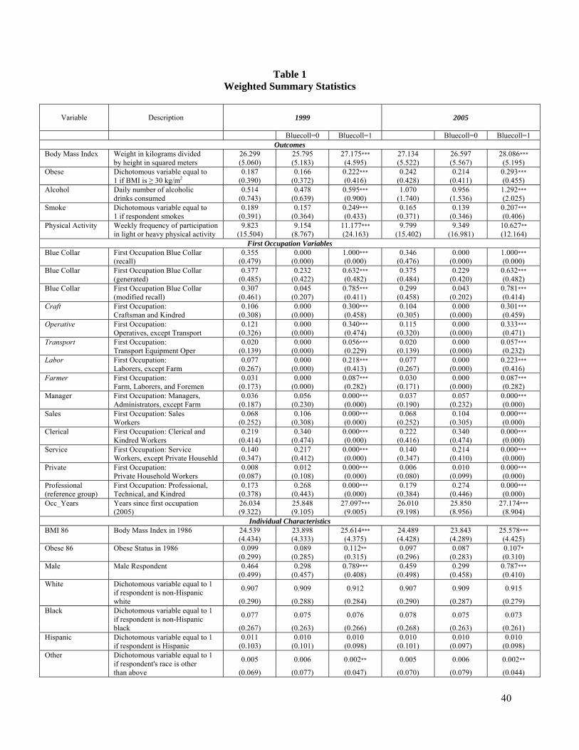
40

Table 1 Weighted Summary Statistics

Variable Description

1999

2005

Bluecoll=0 Bluecoll=1 Bluecoll=0 Bluecoll=1 Outcomes

Body Mass Index Weight in kilograms divided 26.299 25.795 27.175*** 27.134 26.597 28.086*** by height in squared meters (5.060) (5.183) (4.595) (5.522) (5.567) (5.195) Obese Dichotomous variable equal to 0.187 0.166 0.222*** 0.242 0.214 0.293*** 1 if BMI is ≥ 30 kg/m2 (0.390) (0.372) (0.416) (0.428) (0.411) (0.455) Alcohol Daily number of alcoholic 0.514 0.478 0.595*** 1.070 0.956 1.292*** drinks consumed (0.743) (0.639) (0.900) (1.740) (1.536) (2.025) Smoke Dichotomous variable equal to 0.189 0.157 0.249*** 0.165 0.139 0.207*** 1 if respondent smokes (0.391) (0.364) (0.433) (0.371) (0.346) (0.406) Physical Activity Weekly frequency of participation 9.823 9.154 11.177*** 9.799 9.349 10.627** in light or heavy physical activity (15.504) (8.767) (24.163) (15.402) (16.981) (12.164)

First Occupation VariablesBlue Collar First Occupation Blue Collar 0.355 0.000 1.000*** 0.346 0.000 1.000*** (recall) (0.479) (0.000) (0.000) (0.476) (0.000) (0.000) Blue Collar First Occupation Blue Collar 0.377 0.232 0.632*** 0.375 0.229 0.632*** (generated) (0.485) (0.422) (0.482) (0.484) (0.420) (0.482) Blue Collar First Occupation Blue Collar 0.307 0.045 0.785*** 0.299 0.043 0.781*** (modified recall) (0.461) (0.207) (0.411) (0.458) (0.202) (0.414) Craft First Occupation: 0.106 0.000 0.300*** 0.104 0.000 0.301*** Craftsman and Kindred (0.308) (0.000) (0.458) (0.305) (0.000) (0.459) Operative First Occupation: 0.121 0.000 0.340*** 0.115 0.000 0.333*** Operatives, except Transport (0.326) (0.000) (0.474) (0.320) (0.000) (0.471) Transport First Occupation: 0.020 0.000 0.056*** 0.020 0.000 0.057*** Transport Equipment Oper (0.139) (0.000) (0.229) (0.139) (0.000) (0.232) Labor First Occupation: 0.077 0.000 0.218*** 0.077 0.000 0.223*** Laborers, except Farm (0.267) (0.000) (0.413) (0.267) (0.000) (0.416) Farmer First Occupation: 0.031 0.000 0.087*** 0.030 0.000 0.087*** Farm, Laborers, and Foremen (0.173) (0.000) (0.282) (0.171) (0.000) (0.282) Manager First Occupation: Managers, 0.036 0.056 0.000*** 0.037 0.057 0.000*** Administrators, except Farm (0.187) (0.230) (0.000) (0.190) (0.232) (0.000) Sales First Occupation: Sales 0.068 0.106 0.000*** 0.068 0.104 0.000*** Workers (0.252) (0.308) (0.000) (0.252) (0.305) (0.000) Clerical First Occupation: Clerical and 0.219 0.340 0.000*** 0.222 0.340 0.000*** Kindred Workers (0.414) (0.474) (0.000) (0.416) (0.474) (0.000) Service First Occupation: Service 0.140 0.217 0.000*** 0.140 0.214 0.000*** Workers, except Private Househld (0.347) (0.412) (0.000) (0.347) (0.410) (0.000) Private First Occupation: 0.008 0.012 0.000*** 0.006 0.010 0.000*** Private Household Workers (0.087) (0.108) (0.000) (0.080) (0.099) (0.000) Professional First Occupation: Professional, 0.173 0.268 0.000*** 0.179 0.274 0.000*** (reference group) Technical, and Kindred (0.378) (0.443) (0.000) (0.384) (0.446) (0.000) Occ_Years Years since first occupation 26.034 25.848 27.097*** 26.010 25.850 27.174*** (2005) (9.322) (9.105) (9.005) (9.198) (8.956) (8.904)

Individual CharacteristicsBMI 86 Body Mass Index in 1986 24.539 23.898 25.614*** 24.489 23.843 25.578*** (4.434) (4.333) (4.375) (4.428) (4.289) (4.425) Obese 86 Obese Status in 1986 0.099 0.089 0.112** 0.097 0.087 0.107* (0.299) (0.285) (0.315) (0.296) (0.283) (0.310) Male Male Respondent 0.464 0.298 0.789*** 0.459 0.299 0.787*** (0.499) (0.457) (0.408) (0.498) (0.458) (0.410) White Dichotomous variable equal to 1

if respondent is non-Hispanic 0.907 0.909 0.912 0.907 0.909 0.915

white (0.290) (0.288) (0.284) (0.290) (0.287) (0.279) Black Dichotomous variable equal to 1

if respondent is non-Hispanic 0.077 0.075 0.076 0.078 0.075 0.073

black (0.267) (0.263) (0.266) (0.268) (0.263) (0.261) Hispanic Dichotomous variable equal to 1 0.011 0.010 0.010 0.010 0.010 0.010 if respondent is Hispanic (0.103) (0.101) (0.098) (0.101) (0.097) (0.098) Other Dichotomous variable equal to 1

if respondent's race is other 0.005 0.006 0.002** 0.005 0.006 0.002**

than above (0.069) (0.077) (0.047) (0.070) (0.079) (0.044)

41

Elementary Dichotomous variable equal to 0.034 0.015 0.063*** 0.029 0.011 0.055*** 1 if elementary school educ (0.182) (0.120) (0.242) (0.167) (0.105) (0.227) Some High Dichotomous variable equal to 0.105 0.068 0.162*** 0.101 0.062 0.156*** 1 if some high school educ (0.307) (0.251) (0.369) (0.302) (0.242) (0.363) High Dichotomous variable equal to 0.370 0.336 0.426*** 0.364 0.331 0.420*** 1 if high school education (0.483) (0.473) (0.495) (0.481) (0.471) (0.494) Some College Dichotomous variable equal to 0.224 0.232 0.218 0.228 0.235 0.230 1 if some college education (0.417) (0.422) (0.413) (0.420) (0.424) (0.421) College Dichotomous variable equal to 0.267 0.349 0.131*** 0.277 0.361 0.139*** 1 if college education (0.442) (0.477) (0.338) (0.448) (0.480) (0.346) Age Age of respondent (in years) 48.997 48.274 49.907*** 54.266 53.669 55.291*** (14.493) (14.207) (14.435) (13.751) (13.390) (13.920) Single Dichotomous variable equal to 0.055 0.064 0.039*** 0.048 0.055 0.031*** 1 if respondent is single (0.228) (0.245) (0.193) (0.213) (0.227) (0.174) Married Dichotomous variable equal to 0.765 0.754 0.790*** 0.752 0.747 0.776** 1 if respondent is married (0.424) (0.431) (0.407) (0.432) (0.435) (0.417) Widowed Dichotomous variable equal to 0.062 0.065 0.048*** 0.077 0.079 0.063** 1 if respondent is widowed (0.241) (0.246) (0.213) (0.266) (0.270) (0.244) Divorced Dichotomous variable equal to 0.119 0.117 0.123 0.124 0.119 0.130 1 if respondent is divorced or

separated (0.323) (0.321) (0.329) (0.329) (0.324) (0.336)

Employed Dichotomous variable equal to 0.694 0.696 0.713 0.674 0.683 0.680 1 if respondent is employed (0.461) (0.460) (0.452) (0.469) (0.465) (0.467) Household Income Household Income 74196.290 81946.790 62402.600*** 89938.880 97321.200 78835.200*** (in thousands of dollars) (85220.890) (96964.200) (59907.770) (145408.400) (126957.800) (179404.400) Mother’s Educ. Mother’s Education (Category) 3.989 4.219 3.619*** 4.026 4.261 3.634*** (1=grades 0-5, .., 8=college) (1.645) (1.650) (1.544) (1.637) (1.639) (1.533) Father’s Educ Father’s Education (Category) 3.966 4.272 3.437*** 4.009 4.315 3.461*** (1=grades 0-5, .., 8=college) (1.948) (1.985) (1.747) (1.953) (1.982) (1.760) Parents Poor Dichotomous variable equal to 0.266 0.232 0.323*** 0.259 0.225 0.318*** 1 if respondent answered that

growing up, parents were poor (0.442) (0.422) (0.468) (0.438) (0.418) (0.466)

Instrumental VariablesCounty Unemp. County Unemployment Rate in 4.046 3.944 4.204*** 4.049 3.949 4.207*** (1968) 1968 (2.350) (2.146) (2.613) (2.335) (2.118) (2.630) Father Blue Coll Dichotomous indicator for

whether father’s main occupation was blue-collar

0.460 (0.498)

0.413 (0.493)

0.555*** (0.497)

0.462 (0.499)

0.418 (0.493)

0.551*** (0.497)

Notes: Standard deviations are reported in parentheses. Sample sizes are 6971 (year 1999) and 6303 (year 2005). Italicized occupational variables are classified as blue collar occupations. Asterisks denote that the difference in means by “blue collar” (based on recall) is statistically significant at the following levels: *** p-value≤ 0.01; ** 0.01<p-value≤ 0.05; * 0.05<p-value≤ 0.1.

42

Table 2a Impact of First Occupation on Body Mass Index, 1999

(1) (2) (3) (4) (5) (6) (7) (8) (9)

First Occupation Based on Recall

Generated First Occupation

Modified

Recall

Limited Extended Limited Extended Extended

+ ’86 BMI Limited Extended Extended

+ ’86 BMI Extended

Blue Collar 0.3514* 0.3320 0.2184 0.7330** 0.1031 -0.2509 0.5871* (2.21) (1.47) (1.24) (4.82) (0.45) (1.42) (2.56)

Craft 1.0970** 1.1286** (4.08) (2.98) Operative 1.3761** 0.6962 (5.05) (1.62) Transport 1.0650* 1.4230 (2.14) (1.63) Labor 0.8677** 0.5713 (2.95) (1.41) Farmer 1.1160** 1.0974 (2.82) (1.85) Manager 0.4618 0.7798 (1.27) (1.53) Sales 0.7111* 0.5044 (2.31) (1.13) Clerical 0.5038* 0.4421 (2.08) (1.17) Service 1.5094** 0.8029* (5.62) (2.03) Private 1.9115* 1.0171 (2.39) (0.92) Male 1.2255** 0.8098** 1.2209** 0.8756** -0.7834** 1.2171** 0.9801** -0.6346** 0.8216** (7.86) (3.40) (8.31) (3.81) (4.01) (9.40) (4.68) (3.53) (3.74) Black 2.0560** 2.0078** 2.1860** 2.0485** 1.0349** 2.1057** 2.0492** 0.9821** 2.0529** (11.75) (6.65) (12.72) (6.84) (4.31) (12.48) (6.98) (4.17) (6.88) Hispanic 1.1845 0.9038 1.2065 0.9100 -0.0186 0.8530 0.9296 -0.0461 0.9291 (1.74) (0.79) (1.77) (0.80) (0.02) (1.33) (0.82) (0.04) (0.82) Other -1.2469 -2.6125** -1.3731 -2.7808** -1.1715 -1.6280 -2.8751** -1.4073* -2.7762** (1.49) (2.88) (1.60) (3.02) (1.86) (1.92) (3.13) (2.22) (2.91) Some High -1.1232* -1.1970 -1.1393* -1.1529 -0.9552 -1.0264* -1.1554 -0.9726 -1.0876 (2.49) (1.29) (2.53) (1.22) (1.15) (2.38) (1.23) (1.18) (1.14) High -1.2713** -1.0417 -1.4080** -1.0098 -0.6497 -1.2614** -1.0508 -0.7646 -0.9478 (3.01) (1.16) (3.37) (1.11) (0.80) (3.14) (1.16) (0.95) (1.04) Some College -1.3027** -0.4548 -1.5285** -0.4347 -0.4869 -1.2338** -0.4689 -0.6766 -0.3568 (2.95) (0.50) (3.51) (0.47) (0.59) (2.92) (0.51) (0.83) (0.38) College -1.7614** -0.7098 -2.2942** -0.8868 -0.3108 -1.9182** -0.9988 -0.5740 -0.8118 (3.94) (0.76) (5.27) (0.95) (0.37) (4.53) (1.07) (0.69) (0.86) Occ_Years 0.0265* 0.0062 0.0245* 0.0068 0.0347 0.0202 0.0023 0.0361 0.0129 (2.40) (0.24) (2.20) (0.26) (1.46) (1.51) (0.09) (1.55) (0.50) Age 0.2345** 0.2060** 0.2387** 0.2008* -0.0651 0.2385** 0.2058** -0.0641 0.1921* (6.41) (2.61) (6.48) (2.54) (0.69) (6.30) (2.63) (0.68) (2.45) Age Squared -0.0024** -0.0020** -0.0024** -0.0020** -0.0001 -0.0024** -0.0020** -0.0001 -0.0020** (7.41) (2.80) (7.50) (2.73) (0.10) (7.27) (2.81) (0.14) (2.69) Married -1.1859** -1.1686** -1.2164** -1.1403** -1.0877** -1.0838** -0.9713* -1.0154* -1.0527** (3.90) (2.96) (4.00) (2.90) (2.71) (3.64) (2.50) (2.54) (2.70) Widowed 0.0813 -0.0237 0.1633 0.0935 -1.2111* 0.3237 0.3937 -0.9875 0.1840 (0.18) (0.03) (0.36) (0.11) (2.13) (0.73) (0.49) (1.75) (0.22) Divorced -0.7302* -1.3838** -0.7032* -1.3298** -1.6264** -0.6001 -1.2121** -1.5014** -1.2865** (2.09) (3.12) (2.02) (3.01) (3.73) (1.75) (2.79) (3.46) (2.94) Employed -0.5186** 0.2477 -0.5269** 0.2362 -0.3484 -0.5082** 0.1742 -0.3169 0.1882 (2.65) (0.71) (2.68) (0.68) (1.24) (2.65) (0.51) (1.13) (0.55) Mother Educ -0.0560 -0.0562 -0.0440 -0.0474 -0.0546 -0.0430 (0.69) (0.69) (0.70) (0.59) (0.87) (0.53) Father Educ -0.3183** -0.3313** -0.0471 -0.3438** -0.0524 -0.3297** (4.68) (4.92) (0.88) (5.14) (0.99) (4.92) Parents Poor 0.1567 0.1405 -0.1675 0.1365 -0.1117 0.1059

43

(0.64) (0.57) (0.88) (0.56) (0.59) (0.44) Risk Averse 2

-0.5094 (1.58)

-0.5556 (1.73)

0.2046 (0.80)

-0.5655 (1.77)

0.2166 (0.85)

-0.5894 (1.83)

Risk Averse 3

-0.4530 -0.4913 -0.2036 -0.5718 -0.2473 -0.5201 (1.39) (1.51) (0.76) (1.78) (0.94) (1.60)

Risk Averse 4 -0.5077 -0.5170* -0.0374 -0.5648* -0.0604 -0.5122 (1.92) (1.96) (0.17) (2.17) (0.28) (1.96)

BMI 86 0.8754** 0.8731** (28.87) (29.14) Constant 21.5310** 25.4000** 22.4511** 26.0759** 9.8278** 21.9274** 25.9824** 10.0515** 25.8283** (22.94) (12.52) (24.22) (12.82) (4.19) (23.59) (12.87) (4.31) (12.79) Observations 6315 2711 6315 2711 2013 6583 2767 2050 2730 R-squared 0.09 0.11 0.08 0.11 0.59 0.08 0.11 0.59 0.11 Firstocc p-value

0.00000 0.31501 0.02718 0.14094 0.21554 0.00000 0.65067 0.15596 0.01054

Notes: Coefficients from OLS models are reported, with robust t-statistics in parentheses. Asterisks denote statistical significance as follows: *** p-value≤ 0.01; ** 0.01<p-value≤ 0.05; * 0.05<p-value≤ 0.1. Column 9 uses a definition of blue collar that includes responses on first occupation from 2003 and 2005 surveys, which use the 2000 Census of Population; blue collar categories used are: cleaning/maintenance; farming/fishing/forestry; construction; extraction; install/maintenance/repair; production; and transportation. Risk Averse Category 4 represents individuals who are classified as the most risk-averse; the reference group includes individuals who are least risk-averse or most risk-tolerant.

44

Table 2b Impact of First Occupation on Body Mass Index, 2005

(1) (2) (3) (4) (5) (6) (7) (8) (9)

First Occupation Based on Recall

Generated First Occupation

Modified

Recall

Limited Extended Limited Extended Extended +

’86 BMI Limited Extended Extended

+ ’86 BMI Extended

Blue Collar 0.7518** 0.7201** 0.5927* 0.7436** 0.3084 -0.2974 1.0300** (4.02) (2.70) (2.44) (4.21) (1.17) (1.36) (3.80)

Craft 1.3503** 1.7603** (4.31) (4.07) Operative 1.8395** 1.3532** (5.73) (2.76) Transport 1.6847** 2.1138* (2.84) (2.02) Labor 1.4058** 1.2537** (4.21) (2.78) Farmer 1.1129* 1.4688* (2.50) (2.38) Manager 0.5226 1.0497 (1.20) (1.60) Sales 1.0528** 0.7377 (2.97) (1.54) Clerical 0.6910* 1.0512** (2.52) (2.62) Service 1.2698** 0.9291* (4.13) (2.15) Private 1.5847 1.0983 (1.36) (0.65) Male 0.6385** 0.1503 0.5990** 0.1386 -1.5486** 0.7572** 0.3157 -1.2790** 0.0699 (3.59) (0.53) (3.54) (0.52) (5.98) (5.03) (1.28) (5.72) (0.27) Black 1.9646** 1.9268** 2.0652** 1.9645** 1.0552** 2.0458** 2.0120** 1.0417** 1.9199** (9.23) (5.49) (9.92) (5.64) (3.37) (10.16) (5.85) (3.39) (5.56) Hispanic 0.9854 0.5707 1.0212 0.5988 0.3337 0.9210 0.6753 0.2840 0.6183 (1.39) (0.58) (1.46) (0.62) (0.29) (1.38) (0.69) (0.25) (0.64) Other -1.2674 -2.5916** -1.4392 -2.8774** -1.0951 -1.5498 -2.9873** -1.4236* -2.9063** (1.07) (3.00) (1.20) (3.33) (1.81) (1.37) (3.49) (2.32) (3.16) Some High -0.8287 -1.1292 -0.8025 -1.1150 0.6571 -0.7233 -1.0956 0.6646 -1.0489 (1.45) (0.91) (1.41) (0.89) (0.48) (1.36) (0.88) (0.48) (0.83) High -1.1874* -1.0653 -1.2333* -1.0149 0.7616 -1.1136* -1.0343 0.5858 -0.8726 (2.20) (0.89) (2.32) (0.85) (0.57) (2.21) (0.86) (0.44) (0.72) Some College -1.1804* -0.0471 -1.2989* -0.0194 1.1233 -1.0629* -0.0191 0.8167 0.1550 (2.11) (0.04) (2.35) (0.02) (0.83) (2.02) (0.02) (0.61) (0.13) College -1.8052** -0.5906 -2.2181** -0.8688 1.0472 -2.0177** -1.0141 0.5955 -0.7119 (3.17) (0.48) (4.00) (0.71) (0.77) (3.81) (0.83) (0.44) (0.58) Occ_Years 0.0267* 0.0226 0.0257* 0.0234 0.0333 0.0281 0.0184 0.0378 0.0278 (2.06) (0.77) (1.97) (0.81) (1.04) (1.80) (0.64) (1.19) (0.97) Age 0.2157** 0.1258 0.2197** 0.1203 -0.1940 0.2269** 0.1274 -0.1924 0.1176 (4.16) (1.26) (4.22) (1.20) (1.46) (4.32) (1.29) (1.46) (1.18) Age Squared -0.0023** -0.0016 -0.0024** -0.0015 0.0008 -0.0024** -0.0015 0.0007 -0.0015 (5.49) (1.87) (5.60) (1.82) (0.73) (5.72) (1.87) (0.69) (1.83) Married -1.2365** -1.0868* -1.2659** -1.0302* -0.6370 -0.9297* -0.8003 -0.4810 -0.9368 (3.15) (2.11) (3.23) (2.00) (1.26) (2.44) (1.57) (0.96) (1.83) Widowed -0.2816 -0.0672 -0.2477 0.0277 -0.7658 0.0631 0.2644 -0.6082 0.0294 (0.55) (0.08) (0.49) (0.03) (0.99) (0.13) (0.30) (0.79) (0.03) Divorced -0.8901* -1.2490* -0.8512* -1.1465* -1.0243 -0.5370 -0.9541 -0.8199 -1.0460 (2.06) (2.22) (1.98) (2.05) (1.91) (1.30) (1.73) (1.54) (1.89) Employed -0.3634 -0.0280 -0.3912 -0.0376 0.0096 -0.3483 -0.0020 0.0517 -0.0098 (1.63) (0.08) (1.76) (0.11) (0.03) (1.61) (0.01) (0.18) (0.03) Mother Educ -0.0712 -0.0672 -0.0508 -0.0490 -0.0639 -0.0512 (0.75) (0.70) (0.64) (0.51) (0.81) (0.54) Father Educ -0.3207** -0.3393** -0.0632 -0.3722** -0.0757 -0.3439** (4.14) (4.39) (1.00) (4.77) (1.20) (4.46) Parents Poor 0.0797 0.0478 -0.2086 0.0067 -0.1830 0.0011

45

(0.27) (0.16) (0.87) (0.02) (0.77) (0.00) Risk Averse 2 -0.3724

(0.95) -0.4206

(1.07) 0.3085 (0.94)

-0.4643 (1.18)

0.2986 (0.92)

-0.4735 (1.20)

Risk Averse 3 -0.5118 (1.36)

-0.5324 (1.42)

-0.0717 (0.22)

-0.6828 (1.82)

-0.1262 (0.39)

-0.6099 (1.62)

Risk Averse 4 -0.5206 (1.68)

-0.5222 (1.68)

0.0571 (0.20)

-0.5855 (1.90)

0.0135 (0.05)

-0.4981 (1.61)

BMI 86 0.8484** 0.8502** (20.43) (20.96) Constant 23.1582** 28.3747** 24.0258** 29.3696** 14.5504** 23.0936** 28.9447** 14.6891** 28.6530** (15.81) (9.97) (16.53) (10.35) (4.14) (16.05) (10.26) (4.20) (10.17) Observations 5635 2531 5635 2531 1885 5963 2590 1921 2554 R-squared 0.08 0.10 0.07 0.10 0.51 0.07 0.10 0.50 0.10 Firstocc p-value

0.00001 0.02735 0.00006 0.00707 0.01473 0.00003 0.24380 0.17341 0.00015

Notes: Coefficients from OLS models are reported, with robust t-statistics in parentheses. Asterisks denote statistical significance as follows: *** p-value≤ 0.01; ** 0.01<p-value≤ 0.05; * 0.05<p-value≤ 0.1. Column 9 uses a definition of blue collar that includes responses on first occupation from 2003 and 2005 surveys, which use the 2000 Census of Population; blue collar categories used are: cleaning/maintenance; farming/fishing/forestry; construction; extraction; install/maintenance/repair; production; and transportation. Risk Averse Category 4 represents individuals who are classified as the most risk-averse; the reference group includes individuals who are least risk-averse or most risk-tolerant.

46

Table 3a Impact of First Occupation on Obesity, 1999

(1) (2) (3) (4) (5) (6) (7) (8) (9)

First Occupation Based on Recall

Generated First Occupation

Modified

Recall

Limited Extended Limited Extended Extended + ’86 Obese

Limited Extended Extended + ’86 Obese

Extended

Blue Collar 0.0341** 0.0434* 0.0611* 0.0372** -0.0005 -0.0326 0.0668** (2.64) (2.13) (2.49) (3.14) (0.03) (1.38) (3.35)

Craft 0.0735** 0.1096** (2.69) (2.64) Operative 0.1104** 0.0998* (4.35) (2.47) Transport 0.1117** 0.1567* (2.58) (2.01) Labor 0.0706* 0.0876 (2.45) (1.96) Farmer 0.1013** 0.0394 (2.69) (0.61) Manager 0.0118 0.0458 (0.32) (0.83) Sales 0.0369 0.0474 (1.29) (1.13) Clerical 0.0433 0.0429 (1.94) (1.23) Service 0.0933** 0.0804* (3.96) (2.19) Private 0.1498** 0.1472 (2.60) (1.53) Male 0.0195 0.0029 0.0147 0.0044 -0.0180 0.0204 0.0184 0.0063 -0.0021 (1.51) (0.14) (1.21) (0.22) (0.74) (1.88) (1.00) (0.29) (0.11) Black 0.1262** 0.1284** 0.1352** 0.1343** 0.1014** 0.1335** 0.1339** 0.1023** 0.1323** (9.53) (5.26) (10.27) (5.52) (3.36) (10.31) (5.58) (3.43) (5.43) Hispanic 0.1751* 0.1324 0.1762* 0.1297 0.0266 0.1368* 0.1272 0.0093 0.1286 (2.48) (1.17) (2.49) (1.17) (0.21) (2.08) (1.15) (0.08) (1.16) Other -0.0910 -0.0944 -0.1049 (0.98) (1.02) (1.17) Some High -0.0612* -0.0646 -0.0628* -0.0600 -0.0219 -0.0629* -0.0604 -0.0190 -0.0566 (2.39) (1.06) (2.47) (0.99) (0.29) (2.53) (1.00) (0.25) (0.92) High -0.0738** -0.0628 -0.0820** -0.0606 -0.0362 -0.0815** -0.0684 -0.0550 -0.0541 (2.93) (1.03) (3.32) (1.01) (0.50) (3.34) (1.13) (0.77) (0.89) Some College -0.0530* 0.0021 -0.0664** 0.0030 0.0349 -0.0585* -0.0073 0.0021 0.0117 (2.01) (0.03) (2.59) (0.05) (0.46) (2.27) (0.12) (0.03) (0.18) College -0.0910** -0.0279 -0.1188** -0.0439 0.0427 -0.1135** -0.0636 -0.0043 -0.0351 (3.36) (0.43) (4.71) (0.70) (0.55) (4.45) (1.02) (0.06) (0.55) Occ_Years 0.0021* -0.0019 0.0020* -0.0019 0.0005 0.0014 -0.0024 0.0001 -0.0015 (2.38) (0.88) (2.25) (0.88) (0.17) (1.35) (1.15) (0.05) (0.72) Age 0.0096** 0.0090 0.0099** 0.0089 -0.0083 0.0104** 0.0092 -0.0072 0.0080 (3.07) (1.37) (3.16) (1.36) (0.81) (3.28) (1.42) (0.71) (1.22) Age Squared -0.0001** -0.0001 -0.0001** -0.0001 0.0001 -0.0001** -0.0001 0.0001 -0.0001 (3.85) (1.03) (3.93) (1.05) (0.77) (3.98) (1.09) (0.67) (0.95) Married -0.0889** -0.0876** -0.0907** -0.0868** -0.0917* -0.0774** -0.0720** -0.0768* -0.0768** (4.34) (3.18) (4.43) (3.16) (2.36) (3.84) (2.65) (1.98) (2.81) Widowed -0.0265 -0.0410 -0.0225 -0.0301 -0.1156* -0.0078 0.0002 -0.0948 -0.0200 (0.90) (0.79) (0.76) (0.57) (2.24) (0.26) (0.00) (1.77) (0.38) Divorced -0.0486* -0.0799** -0.0469* -0.0766** -0.1129** -0.0392 -0.0690* -0.1035** -0.0714* (2.31) (2.84) (2.22) (2.73) (3.06) (1.86) (2.46) (2.77) (2.53) Employed -0.0361* 0.0171 -0.0360* 0.0149 0.0100 -0.0367** 0.0104 0.0128 0.0102 (2.55) (0.63) (2.54) (0.55) (0.29) (2.63) (0.38) (0.38) (0.38) Mother Educ -0.0092 -0.0098 -0.0154 -0.0087 -0.0160 -0.0080 (1.28) (1.35) (1.79) (1.22) (1.87) (1.11) Father Educ -0.0161** -0.0170** -0.0118 -0.0188** -0.0143* -0.0178** (2.63) (2.78) (1.64) (3.09) (1.99) (2.91)

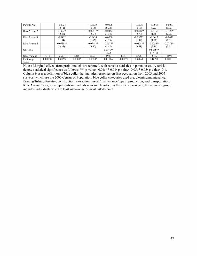
47

Parents Poor -0.0024 -0.0029 -0.0076 -0.0025 -0.0055 -0.0063 (0.12) (0.15) (0.32) (0.13) (0.23) (0.32) Risk Averse 2 -0.0656*

(2.47) -0.0684**

(2.58) -0.0442 (1.33)

-0.0708** (2.70)

-0.0455 (1.38)

-0.0728** (2.76)

Risk Averse 3 -0.0412 (1.54)

-0.0433 (1.63)

-0.0500 (1.53)

-0.0522* (1.99)

-0.0612 (1.90)

-0.0479 (1.81)

Risk Averse 4 -0.0738** (3.35)

-0.0748** (3.40)

-0.0675* (2.47)

-0.0804** (3.68)

-0.0756** (2.80)

-0.0771** (3.51)

Obese 86 0.6646** 0.6635** (16.98) (17.19) Observations 6315 2673 6315 2673 1980 6583 2728 2016 2691 Firstocc p-value

0.00090 0.30195 0.00833 0.03283 0.01286 0.00171 0.97861 0.16701 0.00081

Notes: Marginal effects from probit models are reported, with robust t-statistics in parentheses. Asterisks denote statistical significance as follows: *** p-value≤ 0.01; ** 0.01<p-value≤ 0.05; * 0.05<p-value≤ 0.1. Column 9 uses a definition of blue collar that includes responses on first occupation from 2003 and 2005 surveys, which use the 2000 Census of Population; blue collar categories used are: cleaning/maintenance; farming/fishing/forestry; construction; extraction; install/maintenance/repair; production; and transportation. Risk Averse Category 4 represents individuals who are classified as the most risk-averse; the reference group includes individuals who are least risk-averse or most risk-tolerant.

48

Table 3b Impact of First Occupation on Obesity, 2005

(1) (2) (3) (4) (5) (6) (7) (8) (9)

First Occupation Based on Recall

Generated First Occupation

Modified

Recall

Limited Extended Limited Extended Extended + ’86 Obese

Limited Extended Extended + ’86 Obese

Extended

Blue Collar 0.0682** 0.0671** 0.0913** 0.0477** 0.0133 0.0017 0.0939** (4.57) (2.91) (3.15) (3.52) (0.62) (0.06) (4.13)

Craft 0.1111** 0.1673** (3.55) (3.62) Operative 0.1633** 0.1471** (5.64) (3.24) Transport 0.1686** 0.2244** (3.28) (2.63) Labor 0.1334** 0.1330** (4.01) (2.62) Farmer 0.1199** 0.1570* (2.73) (2.09) Manager 0.0094 0.0402 (0.23) (0.65) Sales 0.0786* 0.0832 (2.41) (1.72) Clerical 0.0719** 0.1136** (2.89) (2.87) Service 0.0949** 0.1019* (3.55) (2.47) Private 0.1309 0.0525 (1.89) (0.51) Male -0.0075 -0.0292 -0.0152 -0.0334 -0.0925** 0.0034 -0.0127 -0.0582* -0.0384 (0.52) (1.23) (1.11) (1.49) (3.27) (0.28) (0.62) (2.30) (1.79) Black 0.1250** 0.1194** 0.1322** 0.1238** 0.1040** 0.1308** 0.1279** 0.1101** 0.1210** (8.05) (4.35) (8.59) (4.53) (3.05) (8.81) (4.75) (3.26) (4.44) Hispanic 0.1163 0.0459 0.1186 0.0468 -0.0105 0.1056 0.0567 -0.0152 0.0455 (1.61) (0.38) (1.65) (0.38) (0.08) (1.57) (0.46) (0.11) (0.37) Other -0.1478 -0.1525 -0.1642 (1.48) (1.54) (1.70) Some High -0.0353 -0.0196 -0.0335 -0.0119 0.0256 -0.0321 -0.0179 0.0170 -0.0041 (1.01) (0.24) (0.96) (0.15) (0.23) (0.96) (0.22) (0.16) (0.05) High -0.0606 -0.0377 -0.0628 -0.0269 0.0077 -0.0598 -0.0325 -0.0060 -0.0133 (1.80) (0.48) (1.88) (0.34) (0.07) (1.85) (0.41) (0.06) (0.17) Some College -0.0459 0.0342 -0.0531 0.0434 0.0740 -0.0460 0.0294 0.0462 0.0606 (1.31) (0.42) (1.54) (0.53) (0.68) (1.36) (0.36) (0.43) (0.73) College -0.0952** -0.0161 -0.1225** -0.0361 0.0680 -0.1184** -0.0575 0.0290 -0.0187 (2.66) (0.20) (3.58) (0.45) (0.62) (3.50) (0.71) (0.27) (0.23) Occ_Years 0.0018 -0.0010 0.0018 -0.0008 -0.0003 0.0012 -0.0006 0.0006 -0.0005 (1.66) (0.40) (1.62) (0.33) (0.10) (0.96) (0.25) (0.16) (0.19) Age 0.0110* 0.0078 0.0113** 0.0071 -0.0012 0.0121** 0.0074 -0.0026 0.0068 (2.56) (0.90) (2.63) (0.82) (0.08) (2.83) (0.87) (0.18) (0.80) Age Squared -0.0001** -0.0001 -0.0001** -0.0001 -0.0000 -0.0001** -0.0001 -0.0000 -0.0001 (3.80) (1.18) (3.89) (1.12) (0.31) (3.95) (1.17) (0.25) (1.12) Married -0.0472 -0.0141 -0.0498* -0.0124 0.0070 -0.0314 0.0009 0.0255 -0.0051 (1.89) (0.42) (2.00) (0.37) (0.14) (1.29) (0.03) (0.53) (0.15) Widowed 0.0223 0.0298 0.0237 0.0362 0.0302 0.0370 0.0501 0.0431 0.0366 (0.62) (0.50) (0.66) (0.60) (0.42) (1.04) (0.83) (0.58) (0.61) Divorced -0.0245 -0.0169 -0.0226 -0.0114 -0.0103 -0.0031 0.0029 0.0166 -0.0022 (0.92) (0.46) (0.85) (0.31) (0.20) (0.12) (0.08) (0.32) (0.06) Employed -0.0373* -0.0288 -0.0387* -0.0276 -0.0386 -0.0304* -0.0255 -0.0335 -0.0279 (2.33) (1.05) (2.43) (1.02) (1.18) (1.98) (0.95) (1.03) (1.03) Mother Educ -0.0037 -0.0037 -0.0142 -0.0018 -0.0135 -0.0020 (0.45) (0.46) (1.45) (0.22) (1.38) (0.25) Father Educ -0.0184** -0.0202** -0.0142 -0.0230** -0.0167* -0.0212** (2.64) (2.91) (1.71) (3.35) (2.02) (3.06) Parents Poor 0.0129 0.0113 -0.0096 0.0093 -0.0082 0.0063

49

(0.55) (0.48) (0.34) (0.40) (0.30) (0.27) Risk Averse 2 -0.0403

(1.25) -0.0426

(1.33) -0.0137 (0.34)

-0.0466 (1.48)

-0.0202 (0.51)

-0.0471 (1.47)

Risk Averse 3 -0.0595 (1.88)

-0.0588 (1.86)

-0.0662 (1.66)

-0.0685* (2.21)

-0.0770* (1.97)

-0.0646* (2.06)

Risk Averse 4 -0.0333 (1.29)

-0.0321 (1.25)

-0.0098 (0.30)

-0.0389 (1.53)

-0.0171 (0.54)

-0.0332 (1.30)

Obese 86 0.6017** 0.5915** (14.41) (14.44) Observations 5635 2491 5635 2491 1848 5963 2550 1884 2514 Firstocc p-value

0.00001 0.04190 0.00000 0.00366 0.00165 0.00043 0.53615 0.94948 0.00004

Notes: Marginal effects from probit models are reported, with robust t-statistics in parentheses. Asterisks denote statistical significance as follows: *** p-value≤ 0.01; ** 0.01<p-value≤ 0.05; * 0.05<p-value≤ 0.1. Column 9 uses a definition of blue collar that includes responses on first occupation from 2003 and 2005 surveys, which use the 2000 Census of Population; blue collar categories used are: cleaning/maintenance; farming/fishing/forestry; construction; extraction; install/maintenance/repair; production; and transportation. Risk Averse Category 4 represents individuals who are classified as the most risk-averse; the reference group includes individuals who are least risk-averse or most risk-tolerant.

50

Table 4a Impact of First Occupation on Alcohol Consumption (Drinks Per Day), 1999

(1) (2) (3) (4) (5) (6) (7)

First Occupation Based on Recall

Generated First Occupation

Modified

Recall

Limited Extended Limited Extended Limited Extended Extended Blue Collar -0.0045 0.0757* -0.0462* 0.0238 0.0710

(0.18) (2.03) (2.03) (0.70) (1.89) Craft 0.0387 0.0367 (0.89) (0.61) Operative -0.0003 0.0413 (0.01) (0.68) Transport 0.0683 0.0368 (0.78) (0.33) Labor 0.0887 0.1509 (1.71) (1.83) Farmer 0.0008 0.0230 (0.01) (0.18) Manager 0.0104 -0.0253 (0.20) (0.37) Sales 0.0655 0.0021 (1.57) (0.03) Clerical 0.0040 -0.0526 (0.14) (1.23) Service 0.0710 -0.0029 (1.95) (0.05) Private -0.0003 0.1124 (0.00) (0.61) Male 0.3106** 0.2792** 0.3281** 0.2909** 0.3330** 0.3117** 0.2978** (13.20) (7.51) (14.57) (8.39) (16.50) (9.46) (8.71) Black -0.0808** -0.0102 -0.0769** -0.0074 -0.0808** -0.0023 -0.0085 (3.15) (0.23) (3.01) (0.17) (3.25) (0.05) (0.20) Hispanic -0.0705 -0.0742 -0.0683 -0.0727 -0.0723 -0.0768 -0.0780 (0.79) (0.46) (0.78) (0.46) (0.88) (0.48) (0.49) Other -0.0123 -0.0637 -0.0214 -0.0586 -0.0251 -0.0726 -0.0718 (0.12) (0.31) (0.21) (0.29) (0.25) (0.36) (0.35) Some High 0.1532** 0.0579 0.1598** 0.0508 0.1550** 0.0394 0.0484 (2.94) (0.37) (3.12) (0.33) (3.17) (0.26) (0.32) High 0.1505** 0.0298 0.1517** 0.0149 0.1245** -0.0051 0.0153 (3.33) (0.20) (3.47) (0.10) (2.91) (0.04) (0.11) Some College 0.1497** 0.0172 0.1489** 0.0026 0.1217** -0.0188 0.0020 (3.08) (0.12) (3.14) (0.02) (2.59) (0.13) (0.01) College 0.2093** 0.0114 0.1951** 0.0032 0.1531** -0.0198 0.0017 (4.12) (0.08) (4.08) (0.02) (3.19) (0.14) (0.01) Occ_Years -0.0004 0.0061 -0.0005 0.0058 -0.0010 0.0064 0.0060 (0.30) (1.47) (0.34) (1.37) (0.53) (1.56) (1.43) Age 0.0094 -0.0127 0.0095 -0.0122 0.0128* -0.0110 -0.0118 (1.84) (1.05) (1.87) (1.01) (2.35) (0.93) (0.99) Age Squared -0.0001* 0.0001 -0.0001* 0.0001 -0.0001** 0.0001 0.0001 (2.13) (0.92) (2.21) (0.89) (2.81) (0.75) (0.85) Married -0.1465** -0.1419** -0.1497** -0.1446** -0.1630** -0.1252* -0.1380* (3.56) (2.60) (3.65) (2.64) (4.05) (2.33) (2.54) Widowed -0.0551 -0.1377 -0.0541 -0.1338 -0.0597 -0.1350 -0.1291 (0.91) (1.44) (0.90) (1.42) (0.98) (1.48) (1.39) Divorced -0.0370 -0.0763 -0.0387 -0.0798 -0.0540 -0.0666 -0.0742 (0.78) (1.28) (0.82) (1.34) (1.16) (1.14) (1.26) Employed 0.0392 -0.0301 0.0367 -0.0320 0.0279 -0.0262 -0.0311 (1.54) (0.62) (1.45) (0.66) (1.12) (0.54) (0.64) Mother Educ 0.0025 0.0029 0.0012 0.0015 (0.20) (0.23) (0.10) (0.12) Father Educ 0.0139 0.0146 0.0144 0.0153 (1.16) (1.23) (1.26) (1.30) Parents Poor -0.0238 -0.0207 -0.0197 -0.0214 (0.65) (0.57) (0.55) (0.60)

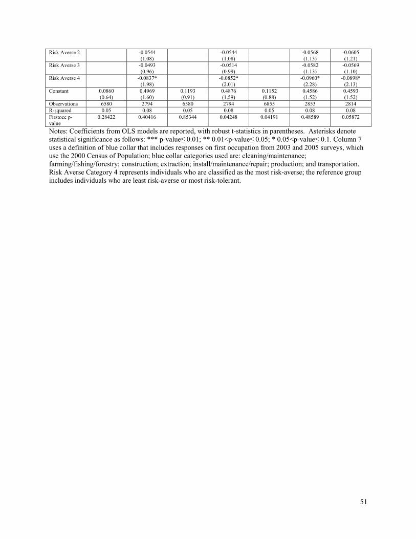
51

Risk Averse 2 -0.0544 -0.0544 -0.0568 -0.0605 (1.08) (1.08) (1.13) (1.21) Risk Averse 3 -0.0493 -0.0514 -0.0582 -0.0569 (0.96) (0.99) (1.13) (1.10) Risk Averse 4 -0.0837* -0.0852* -0.0960* -0.0898* (1.98) (2.01) (2.28) (2.13) Constant 0.0860 0.4969 0.1193 0.4876 0.1152 0.4586 0.4593 (0.64) (1.60) (0.91) (1.59) (0.88) (1.52) (1.52) Observations 6580 2794 6580 2794 6855 2853 2814 R-squared 0.05 0.08 0.05 0.08 0.05 0.08 0.08 Firstocc p-value

0.28422 0.40416 0.85344 0.04248 0.04191 0.48589 0.05872

Notes: Coefficients from OLS models are reported, with robust t-statistics in parentheses. Asterisks denote statistical significance as follows: *** p-value≤ 0.01; ** 0.01<p-value≤ 0.05; * 0.05<p-value≤ 0.1. Column 7 uses a definition of blue collar that includes responses on first occupation from 2003 and 2005 surveys, which use the 2000 Census of Population; blue collar categories used are: cleaning/maintenance; farming/fishing/forestry; construction; extraction; install/maintenance/repair; production; and transportation. Risk Averse Category 4 represents individuals who are classified as the most risk-averse; the reference group includes individuals who are least risk-averse or most risk-tolerant.

52

Table 4b Impact of First Occupation on Alcohol Consumption (Drinks Per Day), 2005

(1) (2) (3) (4) (5) (6) (7)

First Occupation Based on Recall

Generated First Occupation

Modified

Recall

Limited Extended Limited Extended Limited Extended Extended Blue Collar 0.0273 0.0048 -0.0376 -0.0076 -0.0240 (0.50) (0.06) (0.74) (0.09) (0.26) Craft 0.0836 0.0208 (0.88) (0.15) Operative 0.0205 -0.0720 (0.24) (0.54) Transport -0.1653 0.1557 (1.09) (0.53) Labor 0.3918** 0.3462 (3.15) (1.88) Farmer -0.0077 -0.1098 (0.05) (0.34) Manager 0.0510 -0.0589 (0.37) (0.26) Sales 0.2118* 0.2067 (2.15) (1.40) Clerical 0.0430 -0.0225 (0.65) (0.20) Service 0.1010 0.1205 (1.30) (0.95) Private -0.2072 -0.5951** (1.76) (3.49) Male 0.6889** 0.7390** 0.7242** 0.7952** 0.7485** 0.8094** 0.8081** (13.51) (8.50) (14.41) (9.31) (16.40) (10.14) (9.45) Black -0.3990** -0.3211** -0.4022** -0.3154** -0.3840** -0.2809** -0.3227** (6.95) (3.20) (7.09) (3.11) (6.89) (2.77) (3.20) Hispanic 0.1881 0.2263 0.1961 0.2175 0.4095 0.2086 0.2014 (0.68) (0.50) (0.71) (0.49) (1.38) (0.47) (0.46) Other -0.1663 -0.6074 -0.1873 -0.6261 -0.2043 -0.6217 -0.6260 (0.57) (1.17) (0.64) (1.19) (0.73) (1.17) (1.20) Some High 0.1173 0.0947 0.1420 0.1863 0.1841 0.1715 0.1690 (0.90) (0.37) (1.10) (0.73) (1.49) (0.68) (0.66) High 0.1116 0.0252 0.1397 0.1117 0.1484 0.0999 0.1054 (0.90) (0.11) (1.15) (0.47) (1.25) (0.42) (0.44) Some College -0.0022 -0.2593 0.0256 -0.1669 0.0013 -0.1897 -0.1842 (0.02) (1.08) (0.20) (0.71) (0.01) (0.80) (0.78) College -0.0433 -0.2959 -0.0403 -0.2361 -0.0799 -0.2589 -0.2628 (0.33) (1.21) (0.32) (0.99) (0.62) (1.05) (1.08) Occ_Years -0.0012 -0.0103 -0.0014 -0.0112 -0.0035 -0.0093 -0.0123 (0.40) (1.04) (0.48) (1.11) (0.88) (0.96) (1.24) Age -0.0425** -0.0142 -0.0429** -0.0162 -0.0376* -0.0180 -0.0144 (2.95) (0.40) (2.97) (0.46) (2.53) (0.52) (0.42) Age Squared 0.0001 -0.0001 0.0001 -0.0000 0.0001 -0.0000 -0.0000 (1.25) (0.19) (1.23) (0.11) (0.94) (0.08) (0.15) Married -0.3806** -0.3705* -0.3912** -0.3762* -0.4392** -0.3798* -0.4003** (3.49) (2.49) (3.58) (2.52) (3.93) (2.54) (2.65) Widowed -0.0434 -0.0939 -0.0468 -0.0934 -0.0981 -0.1013 -0.1136 (0.33) (0.46) (0.36) (0.46) (0.74) (0.49) (0.55) Divorced 0.0496 0.0326 0.0450 0.0263 -0.0094 0.0145 0.0012 (0.41) (0.20) (0.37) (0.16) (0.08) (0.09) (0.01) Employed 0.0346 -0.1161 0.0387 -0.0960 0.0640 -0.0661 -0.0877 (0.54) (1.07) (0.61) (0.90) (1.04) (0.62) (0.83) Mother Educ -0.0414 -0.0394 -0.0349 -0.0410 (1.52) (1.44) (1.29) (1.52) Father Educ 0.0276 0.0285 0.0295 0.0296 (1.11) (1.15) (1.22) (1.21) Parents Poor -0.1732* -0.1684* -0.1757* -0.1698* (2.14) (2.10) (2.23) (2.13)

53

Risk Averse 2 -0.0648 -0.0684 -0.0786 -0.0694 (0.51) (0.54) (0.63) (0.55) Risk Averse 3 -0.2275 -0.2246 -0.2397 -0.2235 (1.82) (1.79) (1.95) (1.80) Risk Averse 4 -0.1913 -0.1906 -0.1889 -0.1795 (1.79) (1.78) (1.79) (1.69) Constant 2.8164** 2.4499* 2.8863** 2.4291** 2.8076** 2.3986* 2.4239** (6.30) (2.57) (6.51) (2.58) (6.37) (2.57) (2.61) Observations 5872 2598 5872 2598 6212 2658 2621 R-squared 0.10 0.12 0.09 0.11 0.09 0.11 0.11 Firstocc p-value

0.00691 0.00250 0.61369 0.95520 0.45946 0.92893 0.79336

Notes: Coefficients from OLS models are reported, with robust t-statistics in parentheses. Asterisks denote statistical significance as follows: *** p-value≤ 0.01; ** 0.01<p-value≤ 0.05; * 0.05<p-value≤ 0.1. Column 7 uses a definition of blue collar that includes responses on first occupation from 2003 and 2005 surveys, which use the 2000 Census of Population; blue collar categories used are: cleaning/maintenance; farming/fishing/forestry; construction; extraction; install/maintenance/repair; production; and transportation. Risk Averse Category 4 represents individuals who are classified as the most risk-averse; the reference group includes individuals who are least risk-averse or most risk-tolerant.

54

Table 5a Impact of First Occupation on Smoking, 1999

(1) (2) (3) (4) (5) (6) (7)

First Occupation Based on Recall

Generated First Occupation

Modified

Recall

Limited Extended Limited Extended Limited Extended Extended

Blue Collar 0.0150 0.0251 0.0317** 0.0357* 0.0052 (1.28) (1.33) (2.88) (2.00) (0.29) Craft 0.0383 0.0601 (1.57) (1.59) Operative 0.0421 0.0572 (1.81) (1.51) Transport 0.0524 0.1022 (1.38) (1.53) Labor 0.0552* 0.0730 (2.11) (1.75) Farmer 0.0185 0.0860 (0.55) (1.35) Manager -0.0245 -0.0403 (0.72) (0.79) Sales 0.0338 0.0342 (1.23) (0.80) Clerical 0.0338 0.0620 (1.53) (1.79) Service 0.0379 0.0462 (1.69) (1.30) Private -0.0022 0.0459 (0.04) (0.51) Male 0.0765** 0.0647** 0.0749** 0.0601** 0.0728** 0.0656** 0.0692** (6.40) (3.18) (6.69) (3.15) (7.36) (3.77) (3.83) Black -0.0152 -0.0354 -0.0134 -0.0336 -0.0192 -0.0265 -0.0341 (1.24) (1.60) (1.10) (1.52) (1.61) (1.21) (1.54) Hispanic -0.0744 -0.0550 -0.0735 -0.0558 -0.0692 -0.0574 -0.0580 (1.58) (0.56) (1.56) (0.57) (1.48) (0.60) (0.60) Other -0.1533* -0.1538* -0.1581* (2.01) (2.02) (2.13) Some High 0.0408 0.0800 0.0461 0.0835 0.0313 0.0763 0.0792 (1.42) (1.23) (1.60) (1.28) (1.14) (1.19) (1.23) High -0.0812** -0.0916 -0.0771** -0.0874 -0.0867** -0.0845 -0.0921 (3.15) (1.66) (3.01) (1.58) (3.49) (1.53) (1.67) Some College -0.1185** -0.1218* -0.1165** -0.1199* -0.1228** -0.1189* -0.1252* (4.79) (2.32) (4.74) (2.28) (5.12) (2.27) (2.41) College -0.1869** -0.2077** -0.1919** -0.2168** -0.1934** -0.2103** -0.2208** (7.71) (4.11) (8.20) (4.37) (8.36) (4.23) (4.49) Occ_Years -0.0003 -0.0010 -0.0003 -0.0010 -0.0009 -0.0005 -0.0010 (0.32) (0.50) (0.32) (0.48) (0.92) (0.28) (0.53) Age 0.0196** 0.0195** 0.0197** 0.0192** 0.0198** 0.0187** 0.0194** (5.56) (2.89) (5.60) (2.85) (5.71) (2.80) (2.90) Age Squared -0.0002** -0.0002** -0.0002** -0.0002** -0.0002** -0.0002** -0.0002** (7.01) (3.57) (7.07) (3.52) (7.19) (3.46) (3.57) Married -0.1045** -0.0851** -0.1063** -0.0861** -0.1150** -0.0889** -0.0861** (5.29) (3.12) (5.38) (3.17) (5.94) (3.33) (3.19) Widowed -0.0216 -0.0164 -0.0232 -0.0171 -0.0382 -0.0378 -0.0186 (0.71) (0.30) (0.77) (0.31) (1.30) (0.72) (0.34) Divorced 0.0231 0.0414 0.0226 0.0418 0.0149 0.0382 0.0462 (1.09) (1.40) (1.08) (1.42) (0.73) (1.32) (1.57) Employed -0.0378** -0.0666* -0.0381** -0.0655* -0.0354** -0.0614* -0.0640* (2.82) (2.33) (2.84) (2.29) (2.66) (2.16) (2.24) Mother Educ -0.0048 -0.0049 -0.0037 -0.0056 (0.70) (0.72) (0.55) (0.83) Father Educ 0.0010 -0.0001 0.0007 -0.0008 (0.17) (0.02) (0.12) (0.14)

55

Parents Poor -0.0168 -0.0173 -0.0139 -0.0160 (0.87) (0.90) (0.73) (0.84) Risk Averse 2 0.0229 0.0229 0.0217 0.0247 (0.83) (0.83) (0.79) (0.89) Risk Averse 3 0.0161 0.0182 0.0135 0.0163 (0.57) (0.65) (0.49) (0.59) Risk Averse 4 0.0416 0.0428* 0.0372 0.0409 (1.92) (1.97) (1.73) (1.89) Observations 6573 2762 6573 2762 6847 2824 2785 Firstocc p-value

0.52375 0.61747 0.19934 0.18416 0.00400 0.04531 0.77501

Notes: Marginal effects from probit models are reported, with robust t-statistics in parentheses. Asterisks denote statistical significance as follows: *** p-value≤ 0.01; ** 0.01<p-value≤ 0.05; * 0.05<p-value≤ 0.1. Column 7 uses a definition of blue collar that includes responses on first occupation from 2003 and 2005 surveys, which use the 2000 Census of Population; blue collar categories used are: cleaning/maintenance; farming/fishing/forestry; construction; extraction; install/maintenance/repair; production; and transportation. Risk Averse Category 4 represents individuals who are classified as the most risk-averse; the reference group includes individuals who are least risk-averse or most risk-tolerant.

56

Table 5b Impact of First Occupation on Smoking, 2005

(1) (2) (3) (4) (5) (6) (7)

First Occupation Based on Recall

Generated First Occupation

Modified

Recall

Limited Extended Limited Extended Limited Extended Extended Blue Collar 0.0062 -0.0024 0.0193 0.0084 -0.0262 (0.53) (0.13) (1.77) (0.48) (1.51) Craft 0.0068 0.0021 (0.29) (0.06) Operative 0.0083 -0.0161 (0.37) (0.47) Transport 0.0233 0.1020 (0.62) (1.55) Labor 0.0298 0.0220 (1.17) (0.58) Farmer 0.0080 0.0927 (0.24) (1.48) Manager 0.0032 -0.0124 (0.10) (0.25) Sales -0.0015 -0.0090 (0.06) (0.24) Clerical 0.0019 0.0154 (0.09) (0.48) Service 0.0175 0.0191 (0.81) (0.58) Private -0.0362 0.0229 (0.75) (0.29) Male 0.0620** 0.0475* 0.0650** 0.0529** 0.0693** 0.0521** 0.0607** (5.26) (2.46) (5.82) (2.90) (7.00) (3.09) (3.48) Black -0.0155 -0.0442* -0.0148 -0.0432* -0.0184 -0.0442* -0.0466* (1.27) (2.06) (1.23) (2.02) (1.56) (2.12) (2.19) Hispanic -0.0746 -0.0835 -0.0734 -0.0799 -0.0857* -0.0825 -0.0805 (1.74) (1.09) (1.70) (0.98) (2.03) (1.01) (0.99) Some High 0.0189 0.0238 0.0213 0.0319 0.0231 0.0301 0.0270 (0.65) (0.37) (0.74) (0.49) (0.83) (0.47) (0.42) High -0.0797** -0.0977 -0.0789** -0.0922 -0.0737** -0.0922 -0.0986 (3.01) (1.70) (3.02) (1.61) (2.88) (1.61) (1.72) Some College -0.1123** -0.1228* -0.1122** -0.1183* -0.1099** -0.1192* -0.1272* (4.45) (2.30) (4.51) (2.21) (4.47) (2.22) (2.40) College -0.1686** -0.1862** -0.1704** -0.1877** -0.1684** -0.1860** -0.1985** (6.80) (3.57) (7.10) (3.64) (7.10) (3.60) (3.89) Occ_Years -0.0004 -0.0002 -0.0004 -0.0002 -0.0007 0.0002 -0.0004 (0.49) (0.10) (0.47) (0.09) (0.75) (0.10) (0.21) Age 0.0182** 0.0167* 0.0181** 0.0160* 0.0181** 0.0149* 0.0166* (4.66) (2.31) (4.64) (2.23) (4.76) (2.09) (2.32) Age Squared -0.0002** -0.0002** -0.0002** -0.0002** -0.0002** -0.0002** -0.0002** (6.18) (3.22) (6.18) (3.13) (6.34) (3.03) (3.21) Married -0.1053** -0.0904** -0.1072** -0.0909** -0.1211** -0.0891** -0.0925** (5.15) (3.15) (5.24) (3.18) (6.08) (3.14) (3.24) Widowed 0.0063 -0.0129 0.0052 -0.0133 -0.0115 -0.0120 -0.0123 (0.22) (0.28) (0.18) (0.29) (0.41) (0.26) (0.26) Divorced 0.0049 0.0277 0.0042 0.0282 -0.0039 0.0283 0.0268 (0.24) (0.94) (0.20) (0.96) (0.20) (0.97) (0.92) Employed -0.0278* -0.0523* -0.0274* -0.0511* -0.0301* -0.0448* -0.0487* (2.15) (2.29) (2.12) (2.24) (2.39) (1.99) (2.15) Mother Educ -0.0183** -0.0178** -0.0175** -0.0186** (2.76) (2.69) (2.68) (2.80) Father Educ 0.0057 0.0049 0.0060 0.0047 (0.99) (0.86) (1.06) (0.83) Parents Poor -0.0050 -0.0061 -0.0027 -0.0049 (0.26) (0.32) (0.14) (0.26) Risk Averse 2 0.0288 0.0270 0.0243 0.0250 (1.09) (1.02) (0.93) (0.95)

57

Risk Averse 3 0.0126 0.0117 0.0090 0.0101 (0.48) (0.45) (0.35) (0.39) Risk Averse 4 0.0189 0.0207 0.0183 0.0198 (0.93) (1.01) (0.91) (0.98) Observations 5841 2567 5841 2567 6180 2627 2590 Firstocc p-value

0.95340 0.67305 0.59429 0.89280 0.07692 0.62849 0.13173

Notes: Marginal effects from probit models are reported, with robust t-statistics in parentheses. Asterisks denote statistical significance as follows: *** p-value≤ 0.01; ** 0.01<p-value≤ 0.05; * 0.05<p-value≤ 0.1. Column 7 uses a definition of blue collar that includes responses on first occupation from 2003 and 2005 surveys, which use the 2000 Census of Population; blue collar categories used are: cleaning/maintenance; farming/fishing/forestry; construction; extraction; install/maintenance/repair; production; and transportation. Risk Averse Category 4 represents individuals who are classified as the most risk-averse; the reference group includes individuals who are least risk-averse or most risk-tolerant.

58

Table 6a Impact of First Occupation on Physical Activity (frequency of light/vigorous), 1999

(1) (2) (3) (4) (5) (6) (7)

First Occupation Based on Recall

Generated First Occupation

Modified

Recall

Limited Extended Limited Extended Limited Extended Extended Blue Collar 1.2917* 0.8384 1.4910* 1.1768* 1.0556 (2.17) (1.48) (2.30) (2.29) (1.80) Craft 2.4834 0.2361 (1.32) (0.29) Operative 0.3401 0.2129 (0.42) (0.20) Transport 0.8045 2.5454 (0.70) (1.20) Labor 1.4411 1.4544 (1.83) (1.30) Farmer 2.9176* 3.5134 (2.13) (1.93) Manager 1.1764 0.5871 (1.31) (0.51) Sales -0.1623 -0.2539 (0.22) (0.27) Clerical -0.3694 -0.4761 (0.72) (0.65) Service 0.3053 0.0208 (0.55) (0.03) Private 2.7320 3.0636 (1.05) (0.87) Male 0.5349 -0.0155 0.8696 0.1603 0.9705 0.1676 0.0670 (1.09) (0.03) (1.46) (0.29) (1.66) (0.32) (0.13) Black -0.5006 0.3504 -0.5288 0.4144 -0.4496 0.5726 0.6573 (1.03) (0.50) (1.00) (0.57) (0.78) (0.78) (0.87) Hispanic -0.6962 -1.6022 -0.8711 -1.3432 -0.7093 -1.3993 -1.2688 (0.66) (1.18) (0.74) (0.92) (0.58) (0.94) (0.88) Other -2.2045** 0.4750 -2.3461** 0.5463 -1.9621* 0.6584 0.5252 (2.61) (0.32) (2.75) (0.36) (2.11) (0.45) (0.34) Some High 0.3384 -1.0817 0.0549 -1.3233 0.5669 -1.5496 -1.1867 (0.18) (0.38) (0.03) (0.47) (0.31) (0.56) (0.43) High 0.2105 -2.1947 -0.1051 -2.5771 0.5842 -2.4142 -2.4102 (0.11) (0.81) (0.05) (0.99) (0.30) (0.92) (0.93) Some College -1.5023 -3.5603 -1.7760 -3.9078 -0.8549 -3.3128 -3.4283 (0.82) (1.30) (0.91) (1.48) (0.46) (1.25) (1.30) College -1.5493 -3.5877 -1.8273 -3.8969 -0.9929 -3.4258 -3.5460 (0.84) (1.29) (0.93) (1.47) (0.54) (1.29) (1.34) Occ_Years -0.0580 -0.0866 -0.0583 -0.0863 -0.1014 -0.0936 -0.0850 (0.94) (1.04) (0.89) (1.04) (1.24) (1.16) (1.04) Age 0.2044 0.2168 0.2007 0.2044 0.2405 0.2263 0.2206 (0.96) (0.93) (0.93) (0.88) (1.06) (1.00) (0.97) Age Squared -0.0014 -0.0016 -0.0013 -0.0015 -0.0013 -0.0016 -0.0017 (0.79) (0.77) (0.76) (0.71) (0.77) (0.79) (0.80) Married -1.7438* -1.2417 -1.6795* -1.2210 -1.2515 -1.0720 -1.0829 (2.53) (1.54) (2.46) (1.52) (1.90) (1.32) (1.33) Widowed -3.1753* -1.2097 -2.9498 -1.0067 -2.9253* -1.2892 -0.8762 (2.06) (0.60) (1.94) (0.49) (1.97) (0.64) (0.42) Divorced -1.2200 -0.7503 -1.1458 -0.7589 -0.8949 -0.6690 -0.7364 (1.49) (0.80) (1.43) (0.81) (1.19) (0.73) (0.80) Employed -2.5994* -1.7767* -2.6040* -1.7944* -2.2774 -1.7340* -1.7635* (2.03) (2.22) (2.01) (2.21) (1.86) (2.18) (2.18) Mother Educ 0.1909 0.1998 0.1791 0.1552 (0.83) (0.88) (0.80) (0.69) Father Educ -0.0459 -0.0441 -0.0542 -0.0418 (0.28) (0.27) (0.34) (0.26) Parents Poor 0.0317 0.0214 -0.0308 -0.1173 (0.05) (0.03) (0.05) (0.18)

59

Riskdummy2 -1.7384* -1.7434* -1.7277** -1.7895** (2.54) (2.57) (2.60) (2.67) Riskdummy3 -0.6711 -0.7323 -0.8567 -0.8000 (1.00) (1.10) (1.31) (1.20) Riskdummy4 -0.1189 -0.0843 -0.0512 -0.0535 (0.20) (0.14) (0.09) (0.09) Constant 8.7729 9.4987 9.0475 9.9578 6.8060 9.0206 9.2728 (1.94) (1.68) (1.90) (1.79) (1.37) (1.62) (1.67) Observations 3543 1722 3543 1722 3705 1761 1738 R-squared 0.01 0.06 0.01 0.05 0.01 0.05 0.05 Firstocc p-value

0.05674 0.42823 0.03020 0.13889 0.02175 0.02187 0.07149

Notes: Coefficients from OLS models are reported, with robust t-statistics in parentheses. Asterisks denote statistical significance as follows: *** p-value≤ 0.01; ** 0.01<p-value≤ 0.05; * 0.05<p-value≤ 0.1. Column 7 uses a definition of blue collar that includes responses on first occupation from 2003 and 2005 surveys, which use the 2000 Census of Population; blue collar categories used are: cleaning/maintenance; farming/fishing/forestry; construction; extraction; install/maintenance/repair; production; and transportation. Risk Averse Category 4 represents individuals who are classified as the most risk-averse; the reference group includes individuals who are least risk-averse or most risk-tolerant.

60

Table 6b Impact of First Occupation on Physical Activity (frequency of light/vigorous), 2005

(1) (2) (3) (4) (5) (6) (7)

First Occupation Based on Recall

Generated First Occupation

Modified

Recall

Limited Extended Limited Extended Limited Extended Extended Blue Collar -0.1763 0.8241 -0.0945 0.2732 0.5822 (0.17) (0.55) (0.12) (0.29) (0.72) Craft -1.5988 -1.7635 (1.35) (0.99) Operative -1.7221 -0.6476 (1.69) (0.44) Transport -2.9583* -3.9303 (2.14) (1.21) Labor 1.5054 4.0395 (0.91) (1.48) Farmer 2.9019 4.5617 (1.34) (1.58) Manager -0.8926 -0.1305 (1.00) (0.11) Sales 1.3768 4.1563 (0.42) (0.78) Clerical -1.1202 -1.3791 (1.48) (1.32) Service -1.0078 -2.0316 (1.20) (1.61) Private 0.4916 -0.3619 (0.25) (0.13) Male 1.7845 1.6432 2.1015* 2.0418 1.9096** 2.2257* 2.2056 (1.80) (1.03) (2.04) (1.25) (2.72) (2.00) (1.85) Black 1.2904 4.9821 1.1650 5.0157 1.0269 4.7855 4.8595 (0.79) (1.08) (0.72) (1.05) (0.69) (1.03) (1.03) Hispanic -1.5870 -2.7300 -1.3344 -2.1715 -1.1631 -2.2820 -2.3505 (1.57) (1.15) (1.33) (0.97) (1.25) (0.99) (1.02) Other -1.9440* -1.3767 -1.9584* -1.8497 -1.9980** -1.9952 -1.9377 (2.15) (0.50) (2.39) (0.62) (2.61) (0.72) (0.70) Some High 2.7443 -0.2167 2.2127 0.3209 1.8867 0.1931 0.1940 (1.80) (0.09) (1.49) (0.14) (1.23) (0.08) (0.08) High 2.0602 0.8221 1.4919 1.1891 1.0581 1.1222 1.0766 (1.63) (0.35) (1.17) (0.50) (0.82) (0.48) (0.45) Some College 2.2569 0.4206 1.7541 0.7840 1.2483 0.6134 0.6716 (1.26) (0.18) (0.95) (0.31) (0.66) (0.24) (0.26) College 0.9755 -2.0557 0.8097 -1.1213 0.5174 -1.3236 -1.3147 (0.79) (0.69) (0.65) (0.41) (0.40) (0.51) (0.51) Occ_Years 0.0719 0.0086 0.0812 0.0289 0.0967* -0.0074 -0.0123 (1.54) (0.11) (1.67) (0.39) (2.08) (0.09) (0.15) Age -0.3872 -1.2499 -0.4095 -1.2967 -0.4914 -1.1808 -1.1704 (1.31) (1.26) (1.35) (1.25) (1.55) (1.14) (1.15) Age Squared 0.0039 0.0140 0.0040 0.0143 0.0046 0.0135 0.0134 (1.32) (1.25) (1.34) (1.24) (1.48) (1.16) (1.17) Married 0.7440 1.7746 0.6379 1.5607 0.6419 1.6629 1.5325 (0.84) (1.10) (0.75) (1.05) (0.86) (1.17) (1.08) Widowed -1.0020 -4.3037 -1.0367 -4.5251 -0.9502 -4.4429 -4.4810 (0.68) (1.14) (0.70) (1.17) (0.61) (1.15) (1.13) Divorced 0.8730 0.1252 0.7078 -0.3022 0.6556 -0.1637 -0.2478 (0.92) (0.14) (0.75) (0.35) (0.77) (0.19) (0.28) Employed -1.8045 -2.6625 -1.8327 -2.7912 -1.7027 -2.7766 -2.7760 (1.84) (1.28) (1.80) (1.27) (1.80) (1.29) (1.24) Mother Educ -0.6121 -0.5267 -0.4982 -0.4927 (1.51) (1.34) (1.26) (1.24) Father Educ 1.0089 1.0388 1.0484 1.0624 (1.03) (1.01) (1.02) (1.03) Parents Poor -1.2951 -1.3461 -1.0909 -1.1376 (1.01) (1.05) (0.84) (0.88)

61

Riskdummy2 -0.9244 -0.7181 -0.6119 -0.6742 (0.94) (0.72) (0.63) (0.68) Riskdummy3 -0.3776 -0.4922 -0.4664 -0.4643 (0.39) (0.56) (0.52) (0.52) Riskdummy4 1.2233 1.2726 1.3631 1.3869 (1.06) (1.06) (1.17) (1.18) Constant 15.3545** 32.6283 15.8567** 32.1561 18.4081** 29.5804 29.1670 (2.83) (1.81) (2.79) (1.71) (3.04) (1.61) (1.61) Observations 3040 1513 3040 1513 3184 1548 1528 R-squared 0.02 0.09 0.01 0.08 0.01 0.08 0.08 Firstocc p-value

0.05747 0.28242 0.86724 0.58499 0.90089 0.77142 0.47300

Notes: Coefficients from OLS models are reported, with robust t-statistics in parentheses. Asterisks denote statistical significance as follows: *** p-value≤ 0.01; ** 0.01<p-value≤ 0.05; * 0.05<p-value≤ 0.1. Column 7 uses a definition of blue collar that includes responses on first occupation from 2003 and 2005 surveys, which use the 2000 Census of Population; blue collar categories used are: cleaning/maintenance; farming/fishing/forestry; construction; extraction; install/maintenance/repair; production; and transportation. Risk Averse Category 4 represents individuals who are classified as the most risk-averse; the reference group includes individuals who are least risk-averse or most risk-tolerant.

Table 7a Constrained Bivariate Probit Estimates

Effect of Blue Collar First Occupation on Obesity

Sample

1999

2005

Model Constraint

First Occupation

Recalled

First Occupation Generated

First Occupation

Recalled

First Occupation Generated

1 Probit (ρ=0) 0.0339* 0.0147 0.0590** 0.0384* (2.17) (0.97) (3.27) (2.21) 2 ρ=0.1 -0.012837 -0.0304* 0.5970 -0.0149

(0.84) (2.02) (0.22) (0.86) 3 ρ=0.2 -0.0585** -0.0756** -0.0501** -0.0681** (3.89) (5.08) (2.87) (3.99) 4 ρ=0.3 -0.1036** -0.1213** -0.1033** -0.1213** (7.06) (8.24) (6.09) (7.23) 5 ρ=0.4 -0.1486 -0.1680** -0.1557** -0.1748** (10.41) (11.59) (9.48) (10.66) 6 ρ=0.5 -0.1940 -0.2162** -0.2076** -0.2285** (14.03) (15.20) (13.16) (14.35) 7 ρ=-0.1 0.0821*** 0.0603*** 0.1150*** 0.0919*** (5.17) (3.95) (6.31) (5.28) 8 ρ=-0.2 0.1321*** 0.1067*** 0.1720*** 0.1457*** (8.22) (6.98) (9.40) (8.39) 9 ρ=-0.3 0.1842*** 0.1545*** 0.2297*** 0.1999*** (11.37) (10.10) (12.61) (11.62)

10 ρ=-0.4 0.2385*** 0.2039*** 0.2881*** 0.2546*** (14.71) (13.37) (16.00) (15.01)

11 ρ=-0.5 0.2953*** 0.2555*** 0.3468*** 0.3096*** (18.31) (16.87) (19.67) (18.66)

12 Sel on obs= -0.0403*** -0.3101*** -0.0071 -0.0671***

Sel on unobs (3.16)

[ρ=0.15] (26.46)

[ρ=0.72] (0.48)

[ρ=0.10] (4.62)

[ρ=0.26] Observations 4596 4454 4137 4052

Notes: Marginal effects are reported. Robust t statistics are reported in parentheses. Asterisks denote statistical significance as follows: *** p-value<0.01; ** 0.01<p-value≤ 0.05; * 0.05<p-value≤ 0.1.

63

Table 7b Constrained Bivariate Probit Estimates

Effect of Blue Collar First Occupation on Smoking

Sample

1999

2005

Model Constraint

First Occupation

Recalled

First Occupation Generated

First Occupation

Recalled

First Occupation Generated

1 Probit (ρ=0) 0.0119 0.0293* 0.0088 0.0226* (1.04) (2.52) (0.77) (1.98) 2 ρ=0.1 -0.0324** -0.0152 -0.0304** -0.0174

(2.90) (1.32) (2.80) (1.58) 3 ρ=0.2 -0.0754** -0.0597** -0.0680** -0.0567** (6.91) (5.22) (6.44) (5.21) 4 ρ=0.3 -0.1175** -0.1046** -0.1050** -0.0966** (11.08) (9.27) (10.21) (8.97) 5 ρ=0.4 -0.1591** -0.1503** -0.1419** -0.1378** (15.49) (13.56) (14.19) (12.94) 6 ρ=0.5 -0.2008** -0.1973** -0.1794** -0.1807** (20.24) (18.20) (18.48) (17.24) 7 ρ=-0.1 0.0581*** 0.0744*** 0.0495*** 0.0621*** (4.97) (6.34) (4.33) (5.54) 8 ρ=-0.2 0.1065*** 0.1203*** 0.0930*** 0.1034*** (8.95) (10.23) (7.94) (9.16) 9 ρ=-0.3 0.1573*** 0.1675*** 0.1396*** 0.1465*** (13.06) (14.23) (11.66) (12.89)

10 ρ=-0.4 0.2106*** 0.2161*** 0.1896*** 0.1919*** (17.37) (18.43) (15.57) (16.82)

11 ρ=-0.5 0.2666*** 0.2664*** 0.2432*** 0.2399*** (22.01) (22.92) (19.77) (21.04)

12 Sel on obs= -0.1655*** [ρ>1]

0.3847*** [ρ>1]

Sel on unobs (14.73)

[ρ=0.52] (36.40)

[ρ=-0.62] Observations 6602 6448 5897 5848

Notes: Marginal effects are reported. Robust t statistics are reported in parentheses. Asterisks denote statistical significance as follows: *** p-value<0.01; ** 0.01<p-value≤ 0.05; * 0.05<p-value≤ 0.1.

Table 8 Instrumental Variables Estimates based on External Instruments

1999

2005

First

Occupation Recalled

First Occupation Generated

First Occupation

Recalled

First Occupation Generated

BMI

Blue Collar 4.690 3.624 3.507 7.730

(4.329) (4.834) (4.000) (7.403) Observations 2507 2554 2399 2452

Overidentification p-value

0.1155 0.0572 0.1024 0.1195

F statistic 3.86 2.63 5.07 1.75

OBESE

Blue Collar 0.308 0.211 0.386 0.722 (0.348) (0.391) (0.345) (0.646)

Observations 2507 2554 2399 2452 Overidentification

p-value 0.2789 0.1442 0.3439 0.3848

F statistic 3.86 2.63 5.07 1.75

ALCOHOL

Blue Collar -1.471** -2.053* -2.422* -3.547 (0.712) (1.135) (1.368) (2.646)

Observations 2586 2636 2463 2517 Overidentification

p-value 0.1579 0.4118 0.6211 0.6354

F statistic 3.95 2.37 4.93 1.78

SMOKING

Blue Collar 0.058 -0.036 0.360 0.631 (0.334) (0.416) (0.321) (0.552)

Observations 2585 2635 2461 2515 Overidentification

p-value 0.2991 0.1882 0.7588 0.9025

F statistic 3.94 2.36 4.99 1.80

PHYSICAL ACTIVITY

Blue Collar -9.216 -11.993 13.275 20.116 (6.031) (9.805) (46.597) (54.880)

Observations 1596 1628 1449 1480 Overidentification

p-value 0.9763 0.6909 0.2321 0.2564

F statistic 5.90 2.84 0.29 0.22

Notes: Extended models are employed. Robust standard errors are reported in parentheses. Asterisks denote statistical significance as follows: *** p-value<0.01; ** 0.01<p-value≤ 0.05; * 0.05<p-value≤ 0.1. Excluded instruments pertain to county unemployment (1968) and father’s blue collar occupation.

65

Table 9 Instrumental Variables Estimates based on Internal Instruments

1999

2005

First

Occupation Recalled

First Occupation Generated

First Occupation

Recalled

First Occupation Generated

BMI

Blue Collar 0.156 1.481** 1.247* 1.851** (0.679) (0.749) (0.753) (0.876) Observations 2720 2777 2536 2596 Overidentification p-value

0.6858 0.9457 0.9843 0.9400

F statistic 16.33 12.13 16.78 11.10

OBESE

Blue Collar 0.013 0.087 0.064 0.113 (0.057) (0.063) (0.061) (0.071) Observations 2720 2777 2536 2596 Overidentification p-value

0.7824 0.5592 0.8717 0.8180

F statistic 16.33 12.13 16.78 11.10

ALCOHOL

Blue Collar 0.219** 0.128 0.207 -0.495* (0.109) (0.108) (0.249) (0.268) Observations 2803 2863 2603 2664 Overidentification p-value

0.5351 0.2723 0.0773 0.2518

F statistic 14.61 13.45 15.46 11.84

SMOKING

Blue Collar 0.035 -0.034 0.027 -0.042 (0.057) (0.057) (0.054) (0.058) Observations 2801 2861 2600 2661 Overidentification p-value

0.6697 0.4607 0.3944 0.1538

F statistic 14.97 13.65 15.38 11.80

PHYSICAL ACTIVITY

Blue Collar 0.589 0.542 5.149* 6.768** (1.326) (0.867) (3.010) (3.217) Observations 1728 1767 1517 1553 Overidentification p-value

0.5047 0.7278 0.0289 0.9244

F statistic 16.12 49.75 16.88 13.02

Notes: Extended models are employed. Robust standard errors are reported in parentheses. Asterisks denote statistical significance as follows: *** p-value<0.01; ** 0.01<p-value≤ 0.05; * 0.05<p-value≤ 0.1.

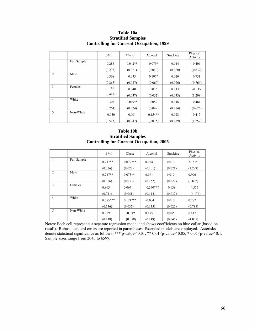
66

Table 10a Stratified Samples

Controlling for Current Occupation, 1999

BMI Obese Alcohol Smoking

Physical Activity

1 Full Sample 0.283

(0.235)

0.042**

(0.021)

0.079*

(0.040)

0.014

(0.020)

0.406

(0.639)

2 Male 0.368

(0.263)

0.033

(0.027)

0.107*

(0.060)

0.020

(0.026)

0.731

(0.764)

3 Females 0.143

(0.482)

0.040

(0.037)

0.016

(0.052)

0.013

(0.033)

-0.315

(1.208)

4 White 0.303

(0.261)

0.049**

(0.024)

0.059

(0.049)

0.016

(0.024)

0.484

(0.626)

5 Non-White -0.050

(0.515)

0.001

(0.047)

0.154**

(0.075)

0.028

(0.039)

0.417

(1.757)

Table 10b

Stratified Samples Controlling for Current Occupation, 2005

BMI Obese Alcohol Smoking Physical Activity

1 Full Sample 0.717**

(0.326)

0.079***

(0.028)

0.024

(0.101)

0.010

(0.021)

2.151*

(1.299)

2 Male 0.717**

(0.326)

0.075**

(0.033)

0.161

(0.152)

0.019

(0.027)

0.996

(0.802)

3 Females 0.803

(0.711)

0.067

(0.051)

-0.340***

(0.114)

-0.039

(0.032)

4.575

(4.174)

4 White 0.885***

(0.336)

0.124***

(0.032)

-0.004

(0.135)

0.010

(0.025)

0.787

(0.788)

5 Non-White 0.209

(0.818)

-0.039

(0.058)

0.175

(0.149)

0.045

(0.045)

6.417

(4.005)

Notes: Each cell represents a separate regression model and shows coefficients on blue collar (based on recall). Robust standard errors are reported in parentheses. Extended models are employed. Asterisks denote statistical significance as follows: *** p-value≤ 0.01; ** 0.01<p-value≤ 0.05; * 0.05<p-value≤ 0.1. Sample sizes range from 2043 to 6599.

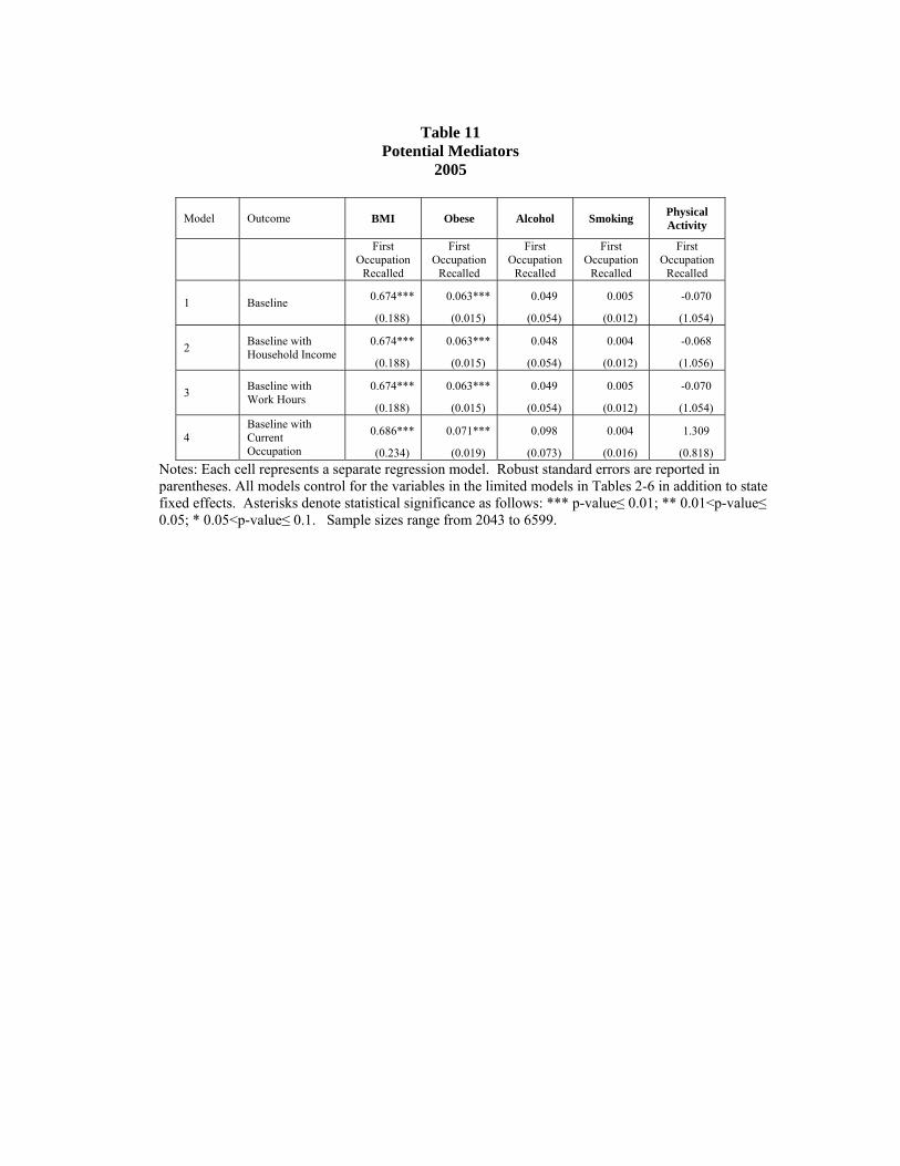
Table 11

Potential Mediators 2005

Model Outcome

BMI

Obese Alcohol Smoking Physical Activity

First

Occupation Recalled

First Occupation

Recalled

First Occupation

Recalled

First Occupation

Recalled

First Occupation

Recalled

1 Baseline 0.674***

(0.188)

0.063***

(0.015)

0.049

(0.054)

0.005

(0.012)

-0.070

(1.054)

2 Baseline with Household Income

0.674***

(0.188)

0.063***

(0.015)

0.048

(0.054)

0.004

(0.012)

-0.068

(1.056)

3 Baseline with Work Hours

0.674***

(0.188)

0.063***

(0.015)

0.049

(0.054)

0.005

(0.012)

-0.070

(1.054)

4 Baseline with Current Occupation

0.686***

(0.234)

0.071***

(0.019)

0.098

(0.073)

0.004

(0.016)

1.309

(0.818)

Notes: Each cell represents a separate regression model. Robust standard errors are reported in parentheses. All models control for the variables in the limited models in Tables 2-6 in addition to state fixed effects. Asterisks denote statistical significance as follows: *** p-value≤ 0.01; ** 0.01<p-value≤ 0.05; * 0.05<p-value≤ 0.1. Sample sizes range from 2043 to 6599.