NBER WORKING PAPERS SERIES

IS THE FISHER EFFECT FOR REAL?A REEXAMINATION OF THE RELATIONSHIP BEThEEN

INFLATION AND INTEREST RATES

Frederic S. Mishkin

Working Paper No. 3632

NATIONAL BUREAU OF ECONOMIC RESEARCH1050 MassachusettS Avenue

Cambridge, MA 02138February 1991

Research support has been provided by the Faculty Research Fund

of the Graduate School of Business, Columbia University. I thank

Ben Bernanke, Ron Gallant, Bruce Greenwald, Jordi Galli, AlastairHall, Kevin Hassett, Ben McCallurn, Pierre Perrofl, Mark Watson andparticipants in seminars at Columbia University, CUNY GraduateCenter, North Carolina State University, Princeton University,Rice University, University of Maryland, and the University OfPennsylvania for helpful comments. The data in this paper will

be made available free of charge to any researcher who sends me astandard formatted 5 1/4w 360KB diskette with a stamped, self -

addressed mailer. This paper is part of NBER's research programin Financial Markets and Monetary Economics. Any opinionsexpressed are those of the author and not those of the National

Bureau of Economic Research.

NBER Working Paper #3632February 1991

IS THE FISHER EFFECT FOR REAL?A REEXAMINATION OF THE RELATIONSHIP BEThEEN

INFLATION AND INTEREST RATES

ABSTRACT

The basic puzzle about the so-called Fisher effect, in which

movements in short-term interest rates primarily reflect

fluctuations in expected inflation, is why a strong Fisher effect

occurs only for certain periods but not for others. This paper

resolves this puzzle by reexamining the relationship between

inflation and interest rates with modern time-series techniques.

Recognition that the level of inflation and interest rates may

contain stochastic trends suggests that the apparent ability of

short-term interest rates to forecast inflation in the postwar

United States is spurious. Additional evidence does not support

the presence of a short-run Fisher effect but does support the

existence of a long-run Fisher effect in which inflation and

interest rates trend together in the long run when they exhibit

trends.

The evidence here can explain why the Fisher effect appears

to be strong only for particular sample periods, but not for

others. The conclusion that there is a long-run Fisher effect

implies that when inflation and interest rates exhibit trends,

these two series will trend together and thus there will be a

strong correlation between inflation and interest rates. On the

other hand, the nonexistence of a short-run Fisher effect implies

that when either inflation and interest rates do not display

trends, there is no long-run Fisher effect to produce a strong

correlation between interest rates and inflation. The analysis

in this paper resolves an important puzzle about when the Fisher

effect appears in the data.

Frederic S. MishkinDepartment of EconomicsFisher HallPrinceton UniversityPrinceton, New Jersey 08544

I. Introduction

The relationship between the level of interest rates and inflation is one

of the most studied topics in economics. A standard view, which is commonly

referred to as the Fisher effect, is that movements in short-term interest rates

primarily reflect fluctuations in expected inflation, so that they havepredictive ability for future inflation. Although the Fisher effect is widely

accepted for the period after the Fed-Treasury Accord in 1951 until October

1979 in the United States,t this relationship between the level of short-term

interest rates and future inflation is not at all robust. The level of short-term

interest rates has no ability to predict future inflation in the United States

prior to World War 112 or in the October 1979 to October 1982 period.3 In

addition, the Fisher effect is not found to be strong for many other countries

even in the postwar period.4

The Fisher effect's lack of robustness raises two issues. First, it leaves

us with the puzzle of why a strong Fisher effect occurs only for certain periods

but not for others. Second, the Fisher effects lack of robustness should make

us somewhat suspicious about its validity.

Recent developments in the time-series econometrics literature help

resolve these two issues and explain why the Fisher effect is not robust. A

large body of current work has focused on testing for stochastic trends in time-

series and has studied the implications of stochastic trends on statistical

'For example, Fama(1975), Nelson and Schwcrt (1977), Mishkin (1981,1988), Fama andGibbons (1982).

1Sce, for example, Barsky (1987), Mishkin (1981) and Summers (1983).

3Sec Fluizinga and Mishkin (1986a).

'Mishkin (1984).

inference. Research beginning with Nelson and Plosser (1982) indicates that

many macroeconomic time series such as interest rates and inflation may he

characterized as having stochastic trends. We are also by now familiar with

the potential for misleading inference when variables have stochastic trends

from the work on the spurious regression phenomenon by Granger andNewbold (1974) and Phillips (1986). Both these lines of research suggest that

the evidence for the Fisher effect in the postwar United States needs to be

reexamined.

This paper conducts such a reexamination and finds that the evidence

does not support a short-run relationship between interest rates and future

inflation. However, the nonexistence of a short-run Fisher effect does not rule

out the possibility that there is a long-run Fisher effect in which inflation and

interest rates share a common trend when they exhibit trends. This paper also

conducts tests for cointegration along the lines of Engle and Granger (1987)

to test for a common trend in interest rates and inflation, and it does find

evidence for a long-run Fisher effect in the postwar U. S. data.

The above evidence resolves the puzzle of why the Fisher effect appears

to be strong in some periods but not in others. The existence of a long-run

Fisher effect implies that when inflation and interest rates exhibit trends,

these two series will trend together and thus there will be a strong correlation

between inflation and interest rates. Just as this analysis predicts, the Fisher

effect appears to be strong in the periods when interest rates and inflationexhibit trends. On the other hand, when these variables do not exhibit trends,

a strong correlation between interest rates and inflation will not appear if

there is noshort-run Fisher effect. Thus the presence of a long-run but not a

short-run Fisher effect predicts that a Fisher effect will not he detectable

SSCC Stock and Watson (1988) for an excellent review of this topic.

during periods when interest rates and inflation do not have trends. It isexactly in these periods that we are unable to detect any evidence for a Fisher

effect.

The next section describes the data used in the empirical analysis,which

is followed by an empirical reexamination of the ability of interest rates to

forecast future inflation. The section following then describes tests for long-

run and short-run Fisher effects, and the paper ends with a set of conclusions.

II. The Data

The empirical analysis makes use of monthly data on inflation rates and

one to twelve-month U.S. Treasury bills for the period February 1964 toDecember 1986.6 The sample starts with February 1964 because this is the

first date that data on all the Treasury bills became available (twelve-monthTreasury bills were not issued until late 1963). End of month T-bill data were

obtained from the Center for Research in Security Prices (CRSP) at theUniversity of Chicago. The one-month bill was defined to have a maturity of

30.4 days, the three-month bill 91.25 days, on up to the twelve month bill with

a maturity of 365 days. For each defined maturity the interest rate wasinterpolated from the two bills that were closest to the defined maturity. In

effect, this means that the slope of the term structure is assumed to beconstant between these two hills.7 The interest rates are expressed on a con-

NoLe that the need for up to twelve-month inflation rates in the empirical analysis requiresCPI data through the end ol 1987.

'Fama (1984) instcad chooscs a bill that has a maturity closest to six months and (hen keeps ontaking the interest ratc from this same bill every month as its maturity shortens in order to getinterest rates on one to six-month hills, in cffcct, Fama is assuming that the slope of the termstructure is flat around the chosen bill. The procedure for data construction in this paper, which

4

tinuously compounded basis at an annual rate in percent as are the inflation

rates. The inflation data are calculated from a CPIseries which appropriately

treats housing costs on a rental-equivalence basis throughout the sample

period. For more details on this series see Huizinga and Mishkin (1984, 1986).

The timing of the variables is as follows. A January interest rate

observation uses the end of December bill rate data. A January observation

for a one-month inflation rate is calculated from the December and January

CPI data; a three-month inflation rate from the December and March CPI

data; and so on.8

III. A Reexamination of theMethodology for Testing the Fisher Effect

In previous work, examination of the Fisher effect has involved testing

for a significant correlation of the level of interest rates and the future

inflation: i.e., testing for the significance of in following regression

equation (which can also be thought of as a forecasting equation).

(1) itT = a,,, + ,,iT

assumes that the slope around the desired maturity is constant rather than zero, makes a lessrestrictive assumption than Fama's procedure. The differences between these two procedures,however, are very slight and make no appreciable difference to the results.

The appropriate dating for the CPI is a particular month is not clear since price quotations onthe component items of the index are collected at different times during the month. As a result,there is some misalignment of the inflation data and the interest rate data which is collected atthe end of the month. In order to see if this misalignment could have an appreciable affect on theresults, I also estimated the regressions in this paper lagging the interest rate data one period(i.e., for the January observation I used the end of November bill rate). The results with thelagged intercst rate data are very similar to those found in the text and none of the conclusionsof the paper changes.

where,= the rn-period future inflation rate from time Ito + m.

iT = the ni-period interest rate known at time .

One way of interpreting this regression is to assume that expectations are

rational as iii Fama (1975). Then it is easy to show that a test of the correla-

tion of interest rates with future inflation is also a test for the correlation of

interest rates and expected inflation.9 Alternatively, we can view thecorrelation of interest rates and future inflation as interesting in its own right.

In this sectionwe will reexamine this methodology for testing the Fisher

effect and show that it does not provide reliable evidence on the existence of

the Fisher effect. The problem with this methodology is that it is subject to

the spurious regression phenomenon described by Granger and Newbold(1974) and Phillips (1986) because both the right and left-hand-side variables

in the regression equation above can he characterized as having unit roots.

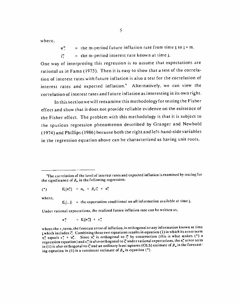
Thc correlation of the level o1 interest rates and expected inflation is examined by testing forthe significance of ,, in the following regression:

() E,[X'J = a,, + iT + u"

where,= the expectation conditional on all information available at timej.

Under rational expectations, the realized future inflation rate can be written as,

= E,(irTI +

where the ,term, the forecast error of inflation, is orthogonal to any information known at time

which includes i'. Combining these two equations results in equation (1) in which its error term

i equals + u. Since u' is orthogonal to i' by construction (this is what makes () aregression equation) and ' is also orthogonal to i" under rational expectations,the v error termin (1) is also orthogonal to iT and an ordinary least squares (OLS) estimate of in the forecast-ing equation in (I) is a consistent estimate of _ in equation ().

()

Table! containstheestimatesoftlieinflationforecastingequationsforhorizons of one, three, six, nine and twelve months.1° Panel A contains the

results for the full sample period, February 1964 to December 1986, while

Panels B, C and D contain the results for three sub-periods, February 1964 to

October 1979, November 1979 to October 1982, and November 1982 to

December 1986. The sample has been split into these three sub-periods

because results in Clarida and Friedman (1984), Huizinga and Mishkin

(1986a) and Roley (1986) suggest that the relationship of nominal interest

rates and inflation shifted with the monetary regime changes of October 1979

and October 1982.

Note that because of serial correlation induced by the use of overlap-

ping data, in which the horizon of the interest rate and the inflation rate is

longer than the one month observation interval, standard errors of the OLS

parameter estimates in equation (1) are generated in the analysis here using

the method outlined by Hansen and Hodrick (1980), with a modification due

to White (1980) and Hansen (1982) that allows for heteroscedasticity'1 and a

modification by Newey and West (1987) that insures the variance-covariance

matrix is positive definite by imposing linearly declining weights on autoco-

°All regression estimates and Monte Carlo results in this paper have been generated with theGAUSS programming language.

"The Hansen (1982) modification is the same numerically as that proposed by White (1980).The Hansen modification applies when there is conditional heteroscedasticity while White'sresults are obtained with unconditional heteroscedasticity rather than conditional hctcrosccdas-ticity, but additional assumptions arc required. The correction [Or hcteroscedasticity is used herebecause Lagrange-multiplier tests outlined by Engle (1982) reject conditional homoscedasticityfor the error term of the forecasting equation. The results were very similar to those reportedin the text when a heteroscedasticity correction was not used in calculating the standard errorsof thc coefficient estimates.

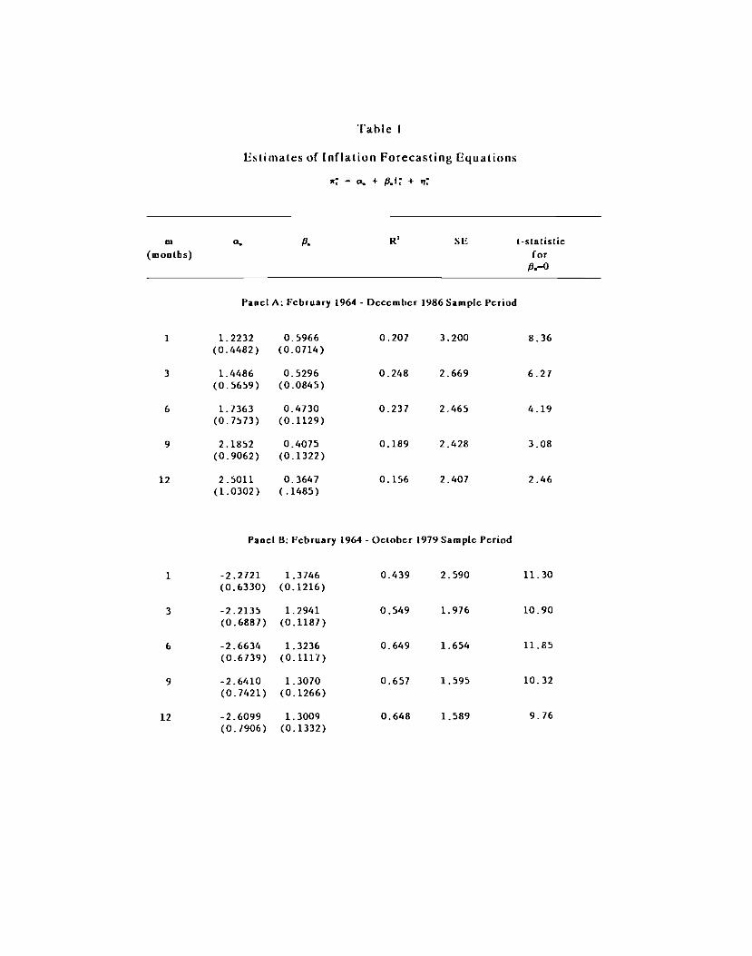
Table I

Estimates of Inflation Forecasting Equations

— a + fl.i +

m a. fl SE t-statistic(mouths) (or

fl.—o

Pancl A: Fcbruary 1964 - Dcccmbcr 1986 Sarnplc Period

1 1.2232 0.5966 0.207 3.200 8.36(0.4482) (0.0714)

3 1.4486 0.5296 0.248 2.669 6.27(0.5659) (0.0845)

6 1.1363 0.4730 0.237 2.465 4.19(0.7573) (0.1129)

9 2.1852 0.4075 0.189 2.428 3.08(0.9062) (0.1322)

12 2.5011 0.3647 0.156 2.407 2.46(1.0302) (.1485)

Panel 14: February 1964 - October 1979 Samplc Pcriod

1 -2.2721 1.3746 0.439 2.590 11.30(0.6330) (0.1216)

3 -2.2135 1.2941 0.549 1.976 10.90(0.6887) (0.1187)

6 -2.6634 1.3236 0.649 1.654 11.85(0.6139) (0.1117)

9 -2.6410 1.3070 0.651 1.595 10.32(0.7421) (0.1266)

12 -2.6099 1.3009 0.648 1.589 9.76(0.1906) (0.1332)

lable I Continued

m a. /L SL t-slatistic(months) for

/3.-.0

Panci C: Novcmbcr 1979- October 1982 Samptc Period

1 1.1035 0.0890 0.005 3498 0.57

(1.8326) (01552)

3 5.0256 0.2353 0.036 2.937 0.93

(3.4120) (0.2526)

6 7.0521 0.0356 0.001 2.674 0.12

(4.1291) (0.2881)

9 10.7631 -0.2785 0.055 2.382 -1.31

(3.3672) (0.2129)

12 10.6754 -0.2918 0.066 2.239 -1.86

(2.7065) (0.1567)

Panci D: Novcmbcr 1982- Dcccmbcr 1986 Sample Period

1 -1.7349 0.6341 0.112 2.474 2.68

(1.9260) (0.2362)

3 -0.1532 0.4054 0.099 L806 2.12(1.6798) (0.1910)

6 1.2817 0.2351 0.077 1.301 1.26

(1.1622) (0.1861)

9 1.8158 0.1706 0.061 1.109 0.95

(1.7911) (0.1803)

12 2.4821 0.092/ 0.024 1.011 0.61(1.5415) (0.1518)

Notcsfor Table 1:

Standard errors of coefficients in parentheses.SE standard crror of the regression.

7

variance matrices.2

The t-statistics for ,. in the last column of Table 1 appear to indicate

that one to twelve month Treasury bill rates contain a highly significant

amount of predictive power for inflation. This finding is especially strong for

the pre-October 1979 sample period (Panel B) where the t-statistics on the ,

coefficient range from 9.76 to 11.85. However, after October 1979. the one

to twelve month interest rates contain much less information about future

inflation. In the October 1979 to October 1982 period of the Fed's nonbor-

rowed reserves target operating procedure. none of the t-statistics exceed

2.0 and in two cases are even negative. Although there is a positive relation-ship between inflation and nominal interest rates at all time horizons in the

post-October 1982 period, the m t-statistics are greater than 2.0 only at time

horizons of one and three months.The results in Table 1 are consistent with earlier findings in the

literature which have examined the relationship between future inflation and

short-term interest rates for a more limited range of time horizons (one to six

months). Using standard critical values of the test statistics, the ability of

short-term interest rates to predict inflation is highly significant. However,

the conclusion that the fi,,, coefficients are statistically significant rests on the

appropriateness of using the t-distribution to conduct statistical inference

with the test statistics found in Table 1. Yet, it is well known that if the

2Notc that in constructing the corrected standard errors, is assumed to have a MA processof order m-1 This is standard practice in the literature, as in Fama (1975), Fama and Bliss

(1987), Huizinga and Mishkin (1984), and Mishkin (1989). However,examination of the residualautocorrelations in the regression estimates here suggest that r' has significant correlationwithits values lagged more than -1 periods. To see if this additional serial correlation has anyeffecton the results, I have calculated the standard errorsfor all the forecasting equationsallowing fornon-zero autocorrelations going back three years (36 periods) andhave conducted Monte Carloexperiments for all the resulting test statistics along the lines described in the text. Allowing

to have a MA process of order 36, does not alter any of the conclusions reached in the text.

variables in a regression contain stochastic trends because their time series

processes have unit roots, then inference with t-distrihutions can he highly

misleading. as has been forcefully demonstrated by Granger and Newbold

(1974) and Phillips (1986).To determine if the levels of inflation and interest rates contain

stochastic trends. Table 2 presents several types of unit root tests for the four

sample periods and time horizons studied in Table 1. The t-test statistic is the

Dickey-Fuller (1979,1981) t-statistic, ( - 1)/s(), from the following

regression:

(2) Y, = k + pY,, + u,

where s() is the OLS standard error of and Y, is the variable being tested

for unit roots. The Z, statistic is a modification of the Dickey-Fuller t-statistic

suggested by Phillips (1987)which allows for autocorrelation and conditional

heteroscedasticity in the error term of the Dickey-Fuller regression. The Z

statistic, also suggested by Phillips (1987), is a similar modification of the test

statistic T(p - 1), where T is the number of observations.'3

As the Monte Carlo simulations in Schwert (1987) point out, the critical

values calculated by Dickey and Fuller for the test statistics in Table 2 can be

very misleading if the time-series models of the variables tested forunit roots

are not pure autoregressive processes but rather include important moving

average terms. This is exactly what is found for the inflation rates examined

here, and therefore it is necessary to obtain the correct small sampledistributions for these test statistics from Monte Carlo simulations which

'The Z and Z, Lest statistics are calculated allowing for 12 non-7cro autocovariances in theerror term of regression (2).

Table 2Unit Root Tests for 7T'' and IT

ifi tTest S(ptistis for 7r TcsI Statistic

t z,

s for i

4 4 4(months)

Panci A: Fcbruary 1964 - Dcccmbcr 1986 Sample Period

1 -7.73 -9.14 -146.96 -2.67 -2.46 -11.22(0.405) (0.348) (0.336) (0.233) (0.351) (0.338)

3 -3.53 -3.21 -18.07 -2.18 -2.13 -8.31

(0.384) (0.353) (0.389) (0.663) (0.738) (0.110)

6 -2.12 -2.28 -8.96 -2.17 -2.10 -8.00

(0.374) (0.310) (0.369) (0.494) (0.544) (0.564)

9 -1.17 -2.18 -7.90 -2.13 -2.07 -7.74(0.295) (0.260) (0303) (0.359) (0.379) (0.358)

12 -1.60 -2.10 -7.30 -2.13 -2.06 -1.65

(0.230) (0.261) (0.292) (0.432) (0.423) (0.420)

Panel B: February 1964 - October 1979 Sample

1 -6.92 -8.43 -124.25 -1.34 -1.41 -6.12

(0.259) (0.273) (0.277) (0.637) (0.537) (0.307)

3 -2.82 -2.56 -11.43 -1.17 -1.36 -5.69(0.193) (0.216) (0.214) (0.594) (0.499) (0.269)

6 -0.99 -1.15 -3.56 -1.20 -1.30 -5.17

(0.606) (0.597) (0.431) (0.624) (0.568) (0.359)

9 -0.66 -1.20 -3.38 -1.09 -1.24 -4.75(0.554) (0.486) (0.371) (0.652) (0.552) (0.330)

12 -0.42 -1.16 -3.11 -1.20 -1.25 -4.16

(0.595) (0.501) (0.357) (0.639) (0.597) (0.392)

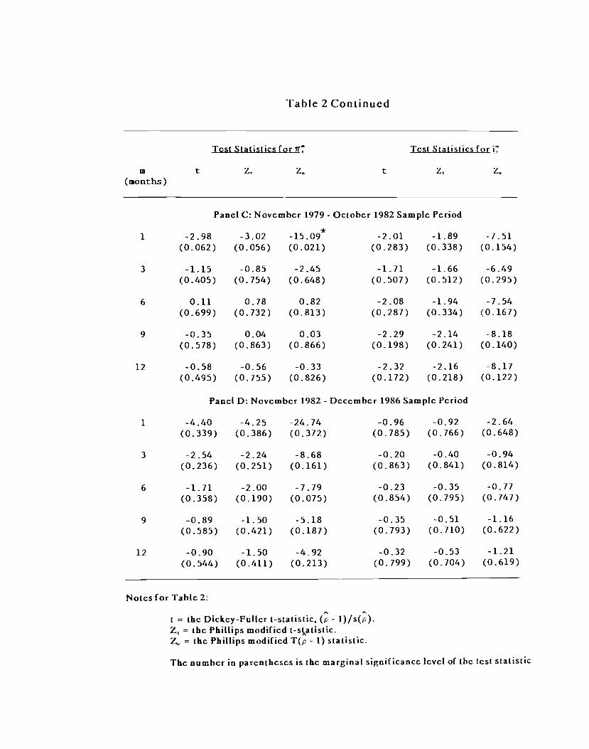
Table 2 Continued

m

Tcst Statistics for

t Z

ir7

Z..

Test Statistics for

t Z

iZ.

(months)

Panci C: Novembcr 1979- October 1982 Sample Period

1 -2.98 -3.02 15.09* -2.01 -1.89 -7.51(0.062) (0.056) (0.021) (0.283) (0.338) (0.154)

3 -1.15 -0.85 -2.45 -1.71 -1.66 -6.49(0.405) (0.754) (0.648) (0.501) (0.512) (0.295)

6 0.11 0.78 0.82 -2.08 -1.94 -7.54(0.699) (0.132) (0.813) (0.287) (0.334) (0.167)

9 -0.35 0.04 0.03 -2.29 -2.14 -8.18

(0.578) (0.863) (0.866) (0.198) (0.241) (0.140)

12 -0.58 -0.56 -0.33 -2.32 -2.16 -8.17

(0.495) (0.755) (0.826) (0.172) (0.218) (0.122)

Panel D: November 1982 - December 1986 Samplc Period

1 -4.40 -4.25 -24.74 -0.96 -0.92 -2.64

(0.339) (0.386) (0.372) (0.785) (0.766) (0.648)

3 -2.54 -2.24 -8.68 -0.20 -0.40 -0.94

(0.236) (0.251) (0.161) (0.863) (0.841) (0.814)

6 -1.71 -2.00 -7.79 -0.23 -0.35 -0.77

(0.358) (0.190) (0.075) (0.854) (0.795) (0.747)

9 -0.89 -1.50 -5.18 -0.35 -0.51 -1.16

(0.585) (0.421) (0.187) (0.793) (0.710) (0.622)

12 -0.90 -1.50 -4.92 -0.32 -0.53 -1.21

(0.544) (0.411) (0.213) (0.799) (0.704) (0.619)

Notes for Table 2:

t = the Dickey-Fuller [-statistic, (p - l)/s(p).= the Phillips modified t.skatistic.

Z. = the Phillips modified T(p - 1) statistic.

The number in parenthcses is thc marginal significance lcvel of the test statistic

calculatcd from Montc Carlo simulations undcr the null hypothesis of a unit root.The number directly under this describes the power of the test statistic: i.e., it is theprobability of rejecting the null of a unit root given the alternative of no unit rootusing thc size corrected 5% critical value for the test statistic.

:.= significant at thc 5% lcvcl.= significant at the 1% lcvcl.

9

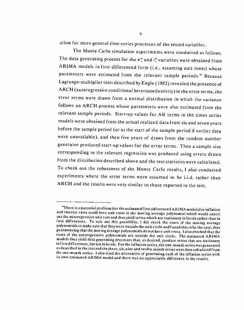
allow for more general time-series processes of the tested variables.The Monte Carlo simulation experiments were conducted as follows.

The data generating process for the itT and iT variables were obtained fromARIMA models in first differenced form (i.e., assuming unit roots) whoseparameters were estimated from the relevant sample periods.t4 Because

Lagrange-multiplier tests described by Engle (1982) revealed the presence ofARCH (autoregressive conditional heteroscedasticity) in the error terms, theerror terms were drawn from a normal distribution in which the variancefollows an ARCH process whose parameters were also estimated from therelevant sample periods. Start-up values for AR terms in the times seriesmodels were obtained from the actual realized data from six and seven years

before the sample period (or at the start of the sample period if earlier datawere unavailable), and then five years of draws from the random number

generator produced start-up values for the error terms. Then a sample size

corresponding to the relevant regression was produced using errors drawn

from the distribution described above and the test statistics were calculated.To check out the robustness of the Monte Carlo results, I also conductedexperiments where the error terms were assumed to be i.i.d. rather thanARCH and the results were very similar to those reported in the text.

There is a potential problem that the estimated first differenced ARIMA modeisfor inflationand interest rates could have unit roots in the movingaverage polynomial which would cancelout the autoregressive Unit root and thus yield series which are stationary in levels rather than infirst differences. To rule out this possibility, I did check the roots of the moving averagepolynomials to make sure that they were outside the unit circle and found this to be thecase, thusguaranteeing that the moving average polynomials do not have unit roots. I also checked that theroots of the autoregressive polynomials arc outside the unit circle. The estimated ARIMAmodels thus yield data generating processes that, as desired, produce series that are stationaryin first differences, but not in levels. For the inflation series, the one-month serieswas generatedas described in the text and the three, six, nine and twelve month scrieswere then calculated fromthe one-month series. 1 also tried the alternative of generating each of the inflation series withits own estimated ARIMA model and there was no appreciable difference in the results.

10

In Table 2 the value in parentheses under the test statistic is the

marginal significance level of the test statistic using the Monte Carlosimulation results described above. The marginal significance levels are the

probability of getting that high a value of the test statistic or higher under the

null hypothesis that the variable has a unit root: i.e., a marginal significance

level less than 0.05 indicates a rejection at the 5% level. As we can see from

the results in Table 2, there is some support for the view that both the levels

of inflation and interest rates contain stochastic trends.'5 In only 1 teststatistic out of 120 in Table 2 do we find a rejection of the null hypothesis of

a unit root. (Interestingly, this rejection occurs during the October 1979 to

September 1982 sample period.)

I have also conducted unit root tests using Augmented Dickey-Fuller

(ADF) tests described by Said and Dickey (1984) in which lags of Y are

included in equation (2) and performed the same Monte Carlo simulation

experiments to obtain the marginal significance levels of these test statistics.

Four different lag lengths were chosen for these ADF tests: two tests used a

procedure similar to that in Perron (1990) in which the lag length was chosen

to be that which produced a t-statistic on the last lagged value of Y that was

significant either at the 10% or the 5% level; one ADF statistic had a fixed lag

length of twelve and the other chose the lag the length with the criterion used

in Schwert (1987) in which the lag length grows with sample size. The results

using these ADF statistics support the findings of Table 2. Just as in Table 2,

only in the October 1979 to September 1982 sample period when in = 1 is

'5This conclusion contrasts with that found in Rose (1988). His rejection of a unit root ininflation arises because he uses the Dickey-Fuller critical values to make his inferences.Howcvcr, as the Monte Carlo results in Schwert (1987) and in Table 2 indicate, using the correctsmall sample distribution to conduct inference does not lead to rejection of a Unit root ininflation.

11

there a rejection of a unit root for inflation, and in no other cases could thenull hypothesis of a unit root in inflation or interest rates be rejected.

The conclusion from Table 2 and the additional Augmented Dickey-Fuller tests is that we cannot reject the null hypothesis that the levels ofinflation and interest rates contain stochastic trends.'6 Thus it is entirelypossible that the inference using the t-distrihution which tells us that interestrates have significant forecasting ability for inflation could be highlymisleading.

To explore this possibility, we again run Monte Carlo simulationexperiments using the procedures described above in which the datagenerating process for the iTT and iT variables was obtained from ARIMAmodels in firstdifferenced form (i.e.,assuming unit roots) using the proceduredescribed earlier. In addition, the error terms from the irT and iT ARIMAmodels are allowed to be contemporaneously correlated as in Mankiw and

Shapiro [1986] and Stambaugh [1986] because this correlation is often found

'The view that interest rates and inflation have stochastic trends in particular sample periodsdoes not imply that there is no tendency to mean reversion in the policy process that generatesmoney growth and inflation rates. In accommodating monetary regimes-- the pre-October 1979period might be characterized as a good example--the conduct of monetary policy could certainlylead to non-stationary behavior of money growth and inflation. However, the high inflation thatsuch a regime creates is likely to lead to a change in regime that would bring inflation back downagain, thus producing a tendency for mean reversion in the long run. Note, however, that thistendency to mean reversion in the long run is consistent with nonstationary behavior within aregime period. Another way to see this point is to recognize that a hyperinflation involves amonetary regime in which money growth and inflation are clearly nonstationary. Yet, at somepoint the problems created by such a high inflation regime will result in a change in monetaryregime which brings the inflation rate back to low levels and leads to mean reversion of inflationin the long run.

12

to he statistically significant.7 The correlation of the error terms is also

estimated using the relevant sample periods. Then a sample size corres-

ponding to the relevant regression was produced using errors drawn from the

distribution described above and the test statistics using the Hansen-Hodrick-

Newey-West-White method allowing for heteroscedasticity described earlier

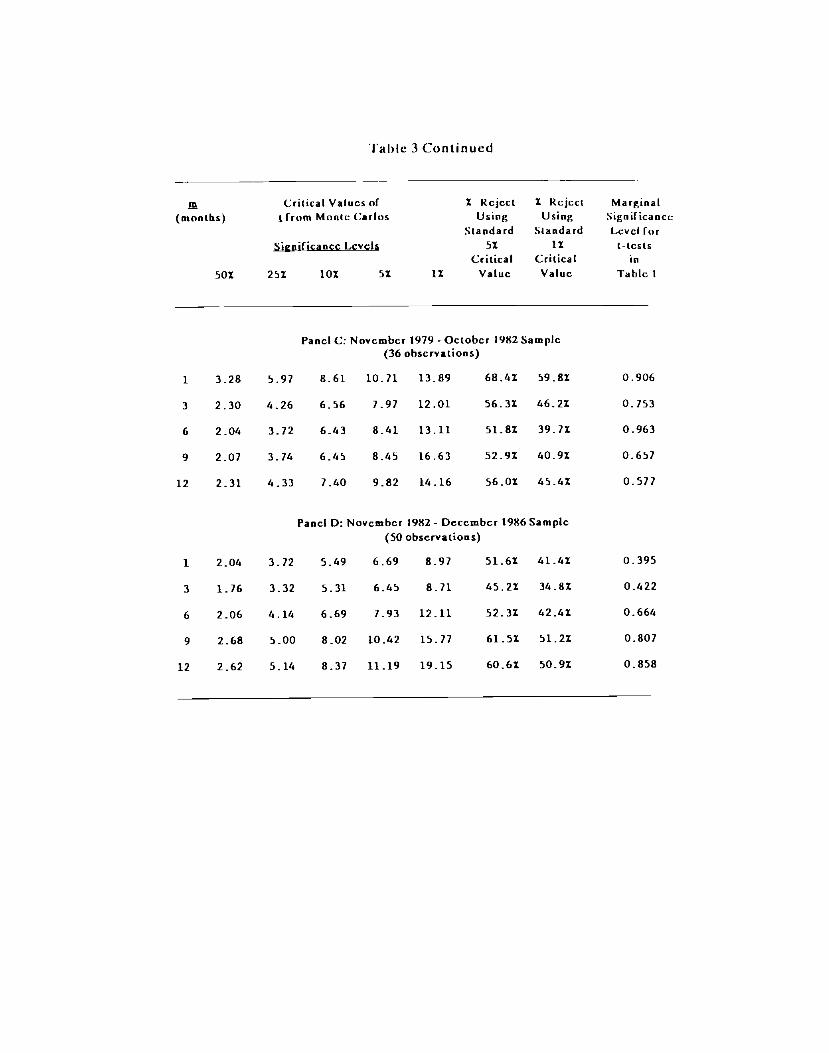
were calculated. Table 3 reports the results of Monte Carlo simulations of one

thousand replications of the t-tests for all the horizons and sample periods in

Table l.The difference between the small sample distribution of these statistics

and that under the t-distrihution is striking. Aswe can see from the results in

columns 7 and 8, the probability of rejecting the null when it is true using

either the t-distribution's 5% or 1% critical value is typically greater than

5Q%1Q Furthermore, as we see from a comparison of Panel A and B with the

shorter sample period results in Panel C and D, the bias does not diminish

"The dating convention for interest rates in this paper is off by one period from theconventional dating used in Mankiw and Shapiro (1986) and Stambaugh (1986). Hence myallowing for contemporaneous correlation of the error terms from the ir and iT ARIMA modelsmeans that I allow for a correlation between the i"-cquation error term and one tag of the yr"-equation error term.

1 also conducted Monte Carlo experiments which 1) added lags of past to the i' ARIMAmodels, 2) assume no correlation of thc error terms from the w" and i' ARIMA models, 3) do notcorrect the test Statistics for hetcroscedasticity, or 4) assume that the error terms are i.i.d. Theseexperiments yield identical conclusions to the Monte Carlo results reported in the text.

'Note that in Table 3 the probability of rejecting the null using the standard critical valuesoften declines as m increases. This reflects the fact that i'has significant autocorrelations forlags greater than ni - 1 although the Hansen-Hodrick-Newey-Wcst-Whitc standard errorcorrection used here, which is standard in the literature, does not allow for non-zero autocorrela-lions for lags greater than rn - 1. When ihc standard error correction allows for non-zeroautocorrelations for up to 36 lags, the Monte Carlo experiments no longer show that theprobability of rejecting the null using the standard critical values declines as increases.

m

(months)

Table 3

Monte Carlo Simulation Resultsfor (-test of 8, = 0

Assuming Unit Roots for 71T and i

50% 25%

Critical Values of 1 Rcjcct 1 Reject MarginalI from Monte Carlos Using

StandardUsing

StandardSignificanccLevel for

Significance Levels 5%

Critical1%

Criticalt-tcsts

in10% 5% 1% Value Value Tabic I

Panci A: February 1964 - December 1986 Sample(275 observations)

1 5.16 9.25 13.66 17.26 24.36 19.21 12.61 0.298

3 3.36 6.03 9.11 1L36 15.76 61.5% 57.81 0.239

6 3.04 5.44 8.31 9.65 13.55 64.41 55.61 0.361

9 2.76 5.09 L90 10.24 15.01 64.51 53.3% 0.443

12 2.76 4.95 7.50 9.55 12.18 61.2% 52.5% 0.542

Panel B: February 1964 - October 1979 Sample(189 observations)

1 8.94 15.48 21.97 25.95 34.84 87.7% 84.3% 0.398

3 6.15 11.58 16.33 19.32 26.08 81.6% 76.0% 0.285

6 5.11 9.23 13.70 16.72 21.99 79.0% 72.4% 0.148

9 5.42 8.96 13.19 15.98 23.50 82.3% 16.0% 0.191

12 4.52 7.76 11.20 13.14 17.24 75.4% 68.6% 0.147

IaI,c 3 Continued

Critical Values of 1 Rcjcct 1 Reject Marginal(months) I Irom Montc Carlos Using Using Signilicancc

Standard Standard Level forSignificancc Lcvcls 51 IX t-tCsts

Ctitical Critical in501 251 lOX 51 IX Value Value Tablc I

Panel C: November 1979- October 1982 Sample(36 observations)

1 3.28 5.91 8.61 10.11 13.89 68.41 59.81 0.906

3 2.30 4.26 6.56 7.97 12.01 56.31 46.21 0./53

6 2.04 3.72 6.43 8.41 13.11 51.81 39.71 0.963

9 2.07 3.16 6.45 8.45 16.63 52.91 40.91 0.657

12 2.31 4.33 7.40 9.82 14.16 56.01 45.41 0.577

Panel 0: Novcmbcr 1982- Dcccmbcr 1986 Sample(SO observations)

1 2.06 3.72 5.49 6.69 8.97 51.61 41.41 0.395

3 1.76 3.32 5.31 6.45 8.11 45.21 34.81 0422

6 2.06 6.14 6.69 7.93 12.11 52.31 42.41 0.664

9 2.68 5.00 8.02 10.42 15.77 61.51 51.21 0.807

12 2.62 5.14 8.37 11.19 19.1S 60.61 50.91 0.858

1 3

appreciably with an increased sample size.7' We also see from the Monte

Carlo 5% critical values of the t-statistics in column 5, that t-statisticsneed to

he greater than 9.5 to indicate a statistically significant ,. coefficient for the

full sample. while they need to exceed 13.0 for the pre-Octoher 1979 sample.

The potential for a spurious regression result between the level of interest

rates and future inflation is thus very high.

The last c&umn of Table 3 indicates that the test results in Table I do

not provide evidence for the forecasting ability of short-term interest rates for

future inflation. This column contains the marginal significance levels for the

t-tests of , = 0 in Table 1 calculated from the Monte Carlo simulations

assuming that the levels of inflation and interest rates have unit roots. These

marginal significance levels are indeed quite high, and for no horizon or

sample period do they indicate that a a,,. coefficient is statistically sig-nificant.21 The results in Table 3, along with the finding that unit roots ininflation and interest rates cannot be rejected, thus indicates that the usual

methodology of regressing the level of inflation on the level of an interest rate

is not able to provide evidence that the level of short-term interest rates has

29ndeed, as Phillips (1986) points out, the bias is likely to increase as the sample size grows.We do see this tendency in the table; the longer Panel A and B samples have greater bias thanthe shorter Panel C and D samples.

2'Using data for one and three month Treasury bills (which arc available before 1959) alongwith the inflation data, 1 also conducted all the tests and Monte Carlo simulations reported inTables ito 4 for the January 1953 to July i71 sample period used in Fama (1975), as well as forthe January 1953 to October 1979 sample period and the January 1953 to December 1986 sampleperiod. The results were very similar to those for the sample periods used in the text. In no casewas the null of a unit root rejected for the interest rate or inflation rate in any of these sampleperiods. Under the assumption of unit root, none of the /3,, coefficients was found to bestatistically significant in any of these sample periods when is assumed to have a MA processor order rn - 1. When t is allowed to have a MA process of order 36, however, a /3 coefficientis Found to be statistically significant in only one case in these sample periods: in the January1953 to July 1971 period when rn = 1, the marginal significance level of the t-statistic on /3,,,calculated from the Monte Carlo simulations assuming unit root is 0.028.

14

any ability to forecast future infIation. Thus we need to look at other

methodologies to examine the relationship between interest rates arid

inflation.

IV. Testing For Long-Run and Short-Run Fisher Effects

The forecasting regression equation in (1) does not make a distinction

between short-run and long-run forecasting ability and hence between short-

run and long-run Fisher effects. An absence of short-run forecasting ability

for interest rates might lead to an inability to reject = 0 in equation (1)

even though higher levels of interest rates are associated with higher levels

of inflation in the long-run. Thus the finding that the regression relationship

between short-term interest rates and future inflation may be spurious if they

have unit roots does not rule out the existence of a long-run Fisher effect in

which inflation and interest rates have a common trend when they exhibit

trends.

Engle and Granger (1987) have demonstrated the linkage between the

presence of common stochastic trends and the conceptof cointegration. If ,r"

and iT are both integrated of order I [denoted by saying that they are 1(1)] then

Note that as Dejong. Nankcrvis, Savin and Whitcrnan (1988) point out, the failure to rejectunit roots may be the result of low power for unit root tests. This conjectureis confirmed for theunit root tests of Table 2 by conducting Monte Carlo simulations. The resulting powercalculations found in the first appendix indeed indicate that the power of the unit root tests isextremely low, rarely getting above one-half. Thus the possibility that the levels of inflation andinterest rates are stationary time series Cannot he ruled out. Monte Carlo simulations for the 1-tests of Table I which assume stationarity rather than unit roots in these series doyield significantrejections of ,. = 0 in thc full sample and the pre-October 1979 sample periods, but not in the

post October 1979 sample periods. Priors that interest ratesand inflation rates arc stationarystochastic variables would then lead to a view that the results in Table I do provide evidenceforthe ability of the level of interest rates toforecast the future level of inflation. However, thisview

would be based on a prior rather than evidence in the data.

15

they are said to he cointegrated of order 1,1 fdenoted by C1(1,1)j if a linear

combination of them is integrated of order zero. In other words n' and i' are

Cl( 1,1). if they are both 1(1) and if is 1(0) in the following so-called

cointegrating regression:

(3) ir'' = + i'' +

Note that this cointegrating regression is identical to the forecastingregressions in (1). Engle and Granger then show that a test for cointegration

involves estimating the cointegrating regression above using ordinary leastsquares (unless,8 is assumed to be known) and then conducting unit root tests

for the regression residual '. In other words, the cointegration of ir'' and i",

which is what we mean by a long-run Fisher effect, implies that a linear

combination of these variables is stationary.

Table 4 presents the results of two sets of cointegration tests using the

Dickey-Fuller t-statistic and the Phillips Z, and Z statistics. The first set

which are found in columns two through four in Table 4 test for a unit root in- i.e., the cointegration tests using the estimated cointegrating

regressions already presented in Table 1. The second set, in columns five

through seven, conduct unit root tests for ir -i' and assume that = 1 in the

cointegrating regression. These latter tests can be characterized [Galli

(1988)1 as testing for a full Fisher effect in which inflation and interest rates

move one-for-one in the long run.

Another way of looking at the second set of tests is to recognize that

they are tests for unit roots in the ex-ante real interest rate under theassumption of rational expectations. This can he demonstrated as follows.

The ex-ante real interest rate for an rn-period bond (rr'") is defined to be:

Table 4

Cointegration Tests

Tcst Statistics for Tcst Statistics for

In t

Unit Root in 7T - i7 Unit Root in ir - i

z z. t z z(months)

Panel A: February 1964 - December 1986 Sample Period

1 -9.16 -ILOS -208.62 -8.75 _10.59* _194.06*(0.270) (0.167) (0.136) (0.068) (0.038) (0.031)

3 -4.08 -3.15 -25.79 -3.98 -3.66 -24.96

(0.338) (0.309) (0.319) (0.222) (0.251) (0.257)

6 -2.47 -2.42 -11.00 -2.70 -2.51 -12.26

(0.452) (0.494) (0.518) (0.286) (0.352) (0.332)

9 -1.97 -2.21 -9.01 -2.36 -2.29 -10.36

(0.433) (0.485) (0.518) (0.239) (0.309) (0.269)

12 -1.64 -2.10 -7.93 -2.06 -2.11 -8.81

(0.456) (0.490) (0.555) (0.386) (0.428) (0.382)

Panel B: February 1964 - October 1979 Sample

1 _10.60* -11.43 -187.94 _9.96* -11.35 -199.71

(0.049) (0.124) (0.227) (0.036) (0.056) (0.094)

* * * *3 -4.68 -4.25 -32.18 -4.44 -4.09 -28.65

(0.033) (0.068) (0.070) (0.019) (0.028) (0.030)

6 379* 343* _21.23* _3.15* -2.19 -14.25

(0.012) (0.036) (0.037) (0.033) (0.102) (0.089)

9 _3.19* -3.02 -16.92 -2.65 -2.49 -11.15(0.042) (0.092) (0.086) (0.062) (0.125) (0.098)

12 -2.90 -2.82 -14.85 -2.35 -2.31 -9.67

(0.083) (0.139) (0.121) (0.108) (0.186) (0.162)

Table 4 Continued

Tcst Statistics for Tcst Statistics for

in

Unit Root in 7r7 - Unit Root in -

t 4 4 t 4 4(months)

Panel C: November 1979- October 1982 Sample Period

1 -2.98 -3.22 17.42* -3.14 3.36* 18.47*(0.162) (0.097) (0.037) (0.055) (0.041) (0.014)

3 -1.43 -1.05 -2.67 -2.01 -1.92 -6.25(0.548) (0.855) (0.861) (0.150) (0.190) (0.106)

6 -0.04 0.57 0.60 -2.02 -1.94 -4.39(0.872) (0.918) (0.948) (0.157) (0201) (0.338)

9 0.15 1.10 0.78 -1.96 -1.87 -4.47(0.805) (0.772) (0.909) (0.191) (0.247) (0.322)

12 -0.27 0.20 0.17 -1.91 -1.85 -4.03

(0.783) (0.934) (0.945) (0.203) (0.235) (0.366)

Panel D: November 1982 - December 1986 Sample Period

1 -4.63 -4.36 -15.10 -4.75 -4.52 -16.81(0.405) (0.455) (0.860) (0.180) (0.253) (0.742)

3 -2.65 -2.16 -7.98 -2.23 -1.76 -6.99(0.312) (0.429) (0.352) (0.348) (0.536) (0.317)

6 -1.56 -1.78 -7.06 -0.98 -1.32 -5.18(0.725) (0.536) (0.292) (0.703) (0.583) (0.298)

9 -0.66 -1.39 -5.13 0.00 -0.54 -1.76(0.815) (0.774) (0.589) (0.858) (0.755) (0.611)

12 -0.74 -1.42 -4.83 -0.05 -0.50 -1.47(0.847) (0.768) (0.676) (0.843) (0.757) (0.646)

Notes for Table 4:

t = the Dickey-Fuller t-statistic, (p - l)/s(p).Z = the Phillips modified t-st,atistic.

= thc Phillips modified T(p - 1) statistic.

The number in parentheses is the marginal significance level of the test statisticcalculated from Monte Carlo simulations under the null hypothesis of a unit root.The number directly under this describes the power of the test statistic: i.e., it is theprobability of rejecting the null of a unit root given thc alternative of no unit rootusing thc size corrected 5% critical value for the test statistic.

:.= significant at the 5% level.= significant at the 1% level.

II 6

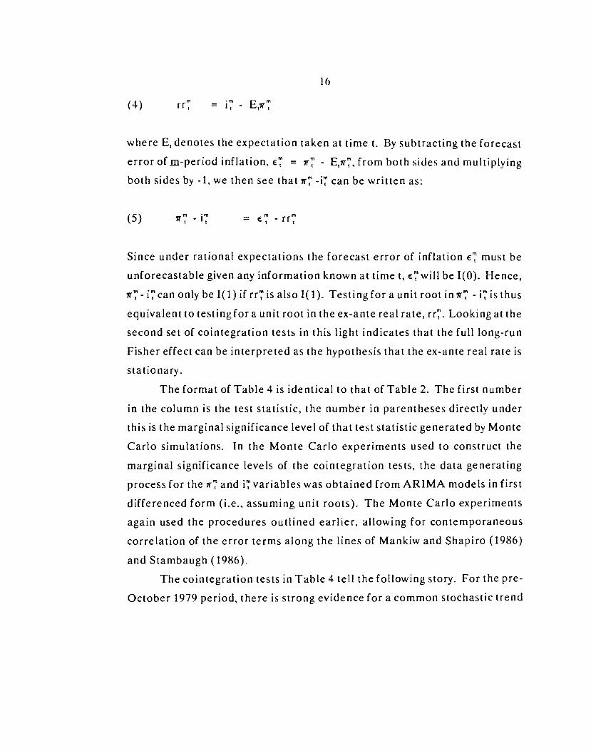
(4) rr" = i" -

where E, denotes the expectation taken at time t. By subtracting the forecast

error of rn-period inflation, €T = ir" - E,irT, from both sides and multiplying

both sides by -1, we then see that ir -iT can be written as:

(5) ir" -i' = €" -rr''

Since under rational expectations the forecast error of inflation ' must he

unforecastable given any information known at time t, 'will be 1(0). Hence,- i' can only be 1(1) if rrT is also 1(1). Testing for a unit root in rT - iT is thus

equivalent to testing for a unit root in the ex-ante real rate, rr". Looking at the

second set of cointegration tests in this light indicates that the full long-run

Fisher effect can be interpreted as the hypothesis that the ex-ante real rate is

Stationary.The format of Table 4 is identical to that of Table 2. The first number

in the column is the test statistic, the number in parentheses directly under

this is the marginal significance level of that test statistic generated by Monte

Carlo simulations. In the Monte Carlo experiments used to construct the

marginal significance levels of the cointegration tests, the data generating

process for the irT and iT variables was obtained from ARIMA models in first

differenced form (i.e., assuming unit roots). The Monte Carlo experimentsagain used the procedures outlined earlier, allowing for contemporaneouscorrelation of the error terms along the lines of Mankiw and Shapiro (1986)

and Stambaugh (1986).

The cointegration tests in Table 4 tell the following story. For the pre-

October 1979 period, there is strong evidence for a common stochastic trend

17

in inflation and interest rates. The null of no cointegration is rejected at the

five percent level using the unit root tests for irT - iT in all the horizons

except twelve months. Similarly unit root tests of ,r' - i' also find support for

cointegration for horizons of one to six months.

There is also evidence for cointegration in the other sample periods of

Table 4, but it is not as strong as for the pre-Octoher 1979 sample period. In

Panel A, C and D we find rejections of unit roots when the horizon is one

month, but notforlonger horizons. However, as Dejong, Nankervis, Savin and

Whiternan (1988) point out the power of these unit root tests may be quitelow and power calculations provided in the first appendix confirms the low

power of the tests in Table 4. Hence the inability to reject unit roots in these

periods should not be viewed as evidence against the existence of a long-run

Fisher effect. Furthermore, using data on one and three month Treasury bills

for the January 1953 to October 1979 and January 1953 to December 1986

sample periods provides strong support for the cointegration of inflation andinterest rates: the null hypothesis of a unit root in irT - i' is always rejected at

the 1% level. Overall, then, the evidence is quite supportive of the existenceof a long-run Fisher effect.23 Indeed, any reasonable model would almost

surely suggest that real interest rates have mean-reverting tendencies, and this

is consistent with the evidence here which supports the existence of a long-

run Fisher effect.The long-run Fisher effect we have found evidence for above tells us

that when the interest rate is higher for a long period of time, then theexpected inflation rate will also tend to be high. A short-run Fisher effect, on

the other hand, indicates that a change in the interest rate is associated with

an immediate change in the expected inflation rate. In other words, we should

'Galli (1988) also comcs to this conclusion.

18

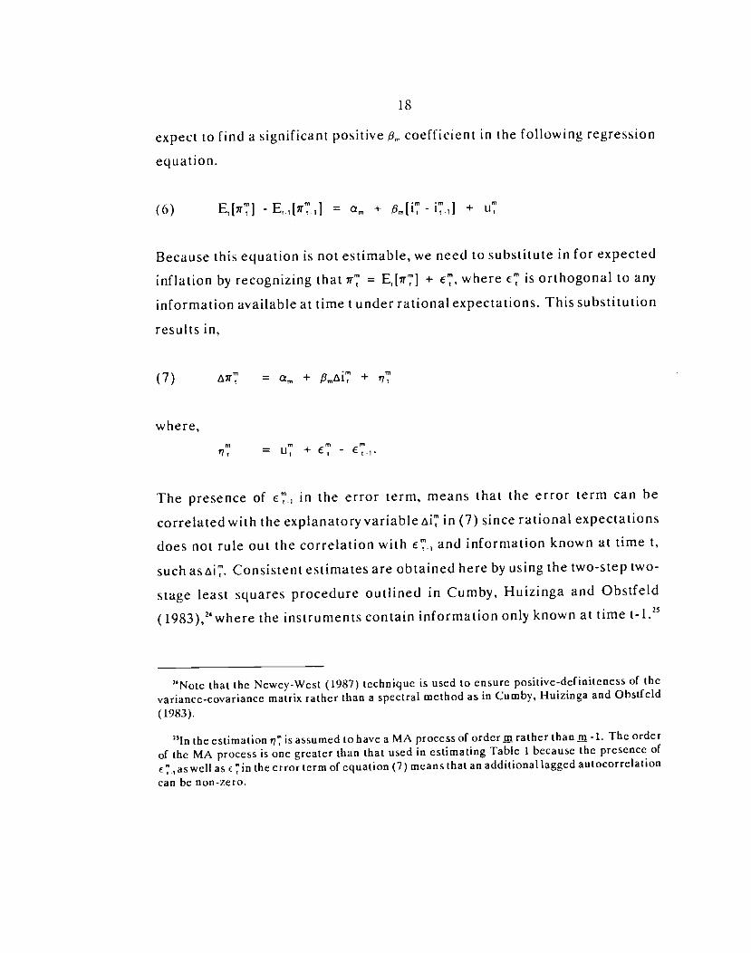
expect to find a significant positive coefficient in the following regression

equation.

(6) E[7r'] - E,.1[ir"1] = + [i7 - i1] + u

Because this equation is not estimable, we need to substitute in for expected

inflation by recognizing that = E[7r'1 + e', where is orthogonal to any

information available at time t under rational expectations. This substitution

results in,

(7) ir' = + +

where,

t7 = u"

The presence of c in the error term, means that the error term can becorrelated with the explanatory variable iT in (7) since rational expectationsdoes not rule Out the correlation with c and information known at time t,

such asiT. Consistent estimates are obtained here by using the two-step two-

stage least squares procedure outlined in Cumby, Huizinga and Obstfeld

(1983),24where the instruments contain information only known at time t-1.25

'Notc that the Newey-West (1987) technique is used to ensure positive-definiteness of thevariance-covariance matrix rather than a spectral method as in Cumby, Huizinga and Ohstfeld(1983).

"In the estimation i is assumed to have a MA process of orderm rather than j -1. The orderof the MA process is one greater than that used in estimating Table 1 because the presence of€7 ,as well as c 7in the error termof equation (7) means that an additional lagged autocorrelationcan he non-zero.

19

Because of the evidence for cointegration, one natural way to choose these

instruments is by estimating error correction models of the type described by

Engle and Granger (1987) in which the variables do not contain information

known after time t-1, and then choose the significant variables from these

models as instruments.

The results from estimating the regression equation above for the

different rn-horizons and sample periods (starting with the January 1965 date

because the need for lagged instruments rules out starting earlier) are found

in Table 5•26 In assessing the statistical significance of the t-statistics on a,,,, we

again conduct Monte Carlo simulations to provide the marginal significance

level of the t-statistic reported in the last column of Table 5. Given the

evidence for cointegration, the data generating process is specified to be one

in which the ir'' and AiT variables are generated from error correction models

in which the current and past values ofiT do not appear in the AT'' equation,

since under the null i' has no forecasting ability for

'Note that the R's from an instrumental variables procedure are not as meaningful as in anOLS regression and arc not guaranteed to be positive. This is why we sometimes see negativeR2s in Table 5.

27Note that these error-correction models differ from the ones used to choose the instrumentsbecause there is no longer the restriction that the explanatory variables in these models must onlycontain information available at time t-1. Also, since the power of the cointegration andunit root

tests is low, we often cannot rule out that r' and i' arc stationary inlevels or have unit roots butwith no cointegration. Since these are also reasonable choices for specificationof the datagenerating process ohr'and i, Monte Carlo simulations have beenconductedfor these twocasesas well using the same procedures described earlier which allow for the contemporaneouscorrelation of error terms. Because ir and do not display much serial correlation in theregression equation (7) above, these Monte Carlo simulations produce similar results. They bothindicate that the t-statistic when m = I in the Panel C sample period is significant at the 5% levelbut not at the 1% level, as is found in TableS. The experiments in which ,r' and i haveunit rootsbut arc not cointegrated indicate that no other t-statistics are statistically significant, just asin

Table S. while the experiments in which ,r' and i' are stationary in levels indicate that only oneother t-statistic is significant at the 5% but not the 1% level (when = 6 in the Panel C sample

period).

Table 5

Tests for Short-Run Fisher Effects

— + fl1 +

m a. 9. SE (-statistic Marginal(months) for Significancc

Lcvcl for(-statistic

Paaci A: January 1965- December 1986 Samplc Pcriod

1 -0.0623 -0.3354 0.001 3.058 -0.65 0.605(0.14-48) (0.5151)

3 0.0075 0.6347 0.016 1.217 2.12 0.066(0.0186) (0.3000)

6 0.0172 0.3265 0.022 0.611 2.07 0.489(0.0433) (0.1574)

9 0.0111 0.0909 0.003 0.407 0.66 0.578(0.0321) (0.1383)

12 0.0263 0.0085 -0002 0.309 0.09 0.951(0.0301) (0.1005)

Panel 8: January 1965- October 1979 Sample Pcriod

1 0.0996 -1.4691 0.003 3.143 -0.71 0.609(0.1971) (1.9069)

3 0.0594 -0.5256 0.002 1.129 -0.63 0.571

(0.0949) (0.8334)

6 0.0339 0.1300 0.000 0.591 0.46 0.853

(0.0478) (0.2835)

9 0.0484 -0.1792 0.005 0.387 -1.01 0.410(0.0310) (0.1610)

12 0.0498 0.06/1 0.001 0.291 0.46 0.688

(0.0380) (0.1461)

Fable S Continued

m a. SE (-statistic Marginal(months) for Signilicancc

Lcvcl br(-Statistic

Panel C: November 1979- Octohcr 1982 Sample Period

1 -0.1849 -0.8378 0.100 2.993 -3.41k 0.025(0.5524) (0.2459)

3 -0.1058 0.1/63 0.022 1.578 1.20 0.503

(0.2304) (0.1465)

6 -0.2211 0.2063 0.063 0.646 2.81 0.014

(0.1066) (0.0735)

9 -0.1960 -0.0099 0.000 0.478 -0.08 0.974

(0.0453) (0.1185)

12 -0.1835 0.0968 0.014 0.285 0.7/ 0.368(0.0441) (0.1255)

Panel D: Novcmber 1982- December 1986 Sample Period

1 -0.1096 0.7023 -0.006 2.779 0.59 0.641(0.3415) (1.1819)

3 0.0179 0.7432 0.007 1.298 0.73 0.545

(0.2104) (1.0140)

6 0.0444 -0.1159 0.001 0.648 -0.15 0.820

(0.1432) (0.7822)

9 0.0273 0.0216 0.000 0.393 0.05 0.956

(0.0852) (0.4803)

12 -0.1158 -1.4405 0.004 0.320 -0.18 0.180

(0.6588) (7.8807)

Notes for Table 5:

Standard errors of coefficients in parentheses.standard error of the regression.

= significant at the 5% level.= significant at the 1% lcvcl.

20

The most striking feature of the Table 5 results is that the ,. coeffi-

cients are as likely to be negative, and thus have the wrong sign for a short-

run Fisher effect, as they are to he positive. Furthermore, only onecoefficient is found to he significantly different from zero (when .rn = 1 in

Panel C) and in this case the coefficient is negative.28 Therefore, there is

absolutely no evidence for the presence of a short-run Fisher effect in theregression results of Table 5. In addition, regression results usingdata on one

and three month Treasury bills for the January 1953 to October 1979 and

January 1953 to December 1986 sample periods also do not reveal any

significant coefficients, and so suggest that there is no short-run Fisher

effect.

V. Interpreting Inflation Forecasting Equations

The conclusion from the preceding empirical analysis is that there isevidence for a long-run Fisher effect but not for a short-run Fisher effect.

This characterization of the inflation and interest rate data along with the

assumption of rational expectations can be used to provide a straightforward

interpretation of when we will be likely to see estimated coefficients

substantially above zero in the inflation forecasting equations. As in Mishkin

(1990). we can derive an expression for the coefficient in the inflation

forecasting equation (1) by writing down the standard formula for theprojection coefficient,, while recognizing that the covariance of the inflation

"Similar rcsultsarcfoundwhcn equation (7) isestimated by OLS rather than by two-step, two-stage least squares. With OLS there arc two significant , coefficients, but again they arcnegative. The fact that OLS yiclds similar conclusions to those n Table 5 suggests that theinability to find a short-run Fisher effect does nor stem from the procedure used here forchoosing instruments.

21

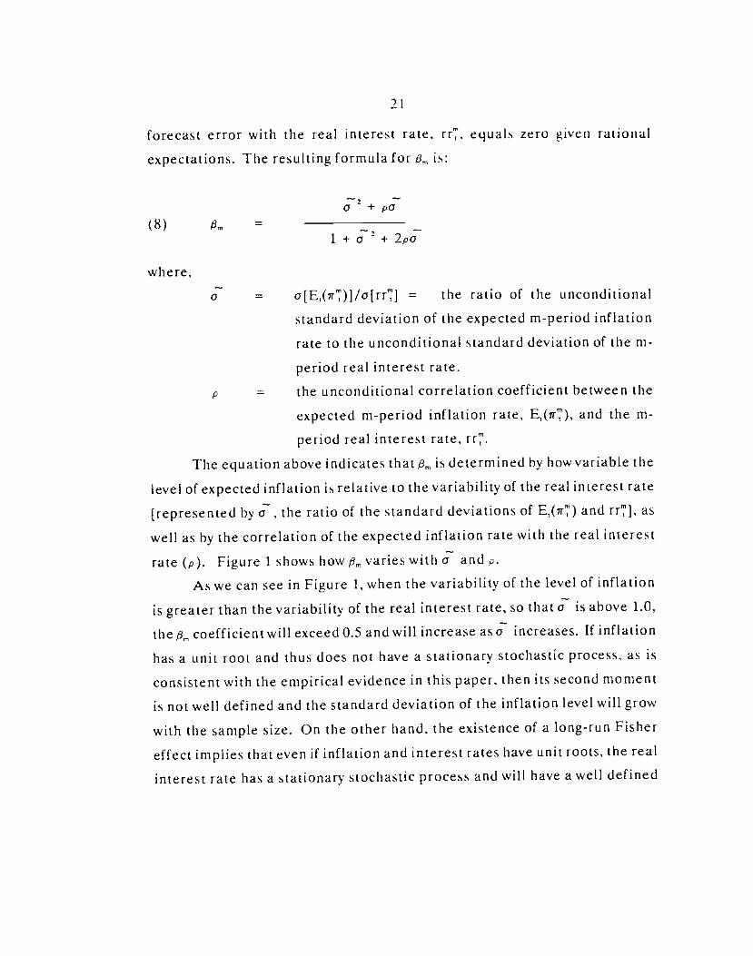
forecast error with the real interest rate. rr'. equals zero given rational

expectations. The resulting formula for is:

(8)1 + a 2 + 2pu

where,

a = o[E,(r')]/a[rr''] = the ratio of the unconditional

standard deviation of the expected rn-period inflation

rate to the unconditional standard deviation of the m-

period real interest rate.

p = the unconditional correlation coefficient between the

expected rn-period inflation rate, E(irT), and the m-

period real interest rate, rr'.

The equation above indicates that 8, is determined by how variable the

level of expected inflation is relative to the variability of the real interest rate

[represented by a, the ratio of the standard deviations of E(ir') and rrT}, as

well as by the correlation of the expected inflation rate with the real interest

rate (p). Figure 1 shows how varies with a and p.

As we can see in Figure 1, when the variability of the level of inflation

is greater than the variability of the real interest rate, so that a is above 1.0.

the coefficient will exceed 0.5 and will increase as a increases. If inflation

has a unit root and thus does not have a stationary stochastic process, as isconsistent with the empirical evidence in this paper. then its second moment

is not well defined and the standard deviation of the inflation level will grow

with the sample size. On the other hand, the existence of a long-run Fisher

effect implies that even if inflation and interest rates have unit roots, the real

interest rate has a stationary stochastic process and will have a well defined

FIG

UR

E

1

U

1.5

1.0

0.5

0.0

—0.

5 1

2 3

standard deviation that does not grow with the sample size. Hence when we

are in sample period in which inflation and interest rates have unit roots, the

existence of a long-run Fisher effect means that o must necessarily exceed

one and produce a value of substantially above zero, as long as the sample

size is large enough.

It is important to note that the reasoning above applies equally well if

inflation and interest rates have a deterministic trend rather than a stochastic

trend. A deterministic trend also implies that the standard deviation of the

inflation level will grow with the sample size. On the other hand, the long-

run Fisher effect of a common deterministic trend for inflation and interest

rates leads to stationary behavior for the real rate so that it has a well defined

standard deviation that does not grow with the sample size. Then thereasoning follows as above.

We now see that a long-run Fisher effect in which inflation and interest

rates have a common trend will produce a,,, substantially above zero in long

samples even when there is substantial variation in the real interest rate.

However, if there is substantial variation in the real rate when we are in a

sample in which inflation is a stationary stochastic variable, the standard

deviation of the real rate might wellexceed the standard deviation in expected

inflation, which is now well defined and does not grow with the sample size.

The result would be a c less than one. Thus in a period when inflation and

interest rates do not have trends, we might expect to find estimated values of

$m that are close to zero.

The above interpretation does help explain the results we have found

in Table 1. We can calculate estimated values of a and p using the procedure

outlined in Mishkin (1981), in which estimates of the real rate. rr'. are

obtained from fitted values of regressions of the ex-post real rate on past

inflation changes and past interest rates.2 Then the estimated expected

inflation is calculated from the following definitional relationship,

(9) E(irT) = i" - rr'

Finally estimates of atE(iT')], o[rrTl, and p are calculated from the estimated

E(rT) and rr'.3°Consistent with the view that inflation has a unit root, which we were

unable to reject except in one instance in the November 1979 - October 1982

sample period, we find that the estimated standard deviation of expected

inflation is much larger for the longer full sample and pre-October 1979sample periods than it is for either of the shorter post-October 1979 sampleperiods. On the other hand, our rejection of a unit root in the real rate,

implies that the standard deviation of the real rate should not necessarily be

larger in the longer sample periods. Again this is exactly what we find: the

post-October 1982 and pre-Octoher 1979 sample periods have standarddeviations of the real rate that are similar in magnitude. However, as isdocumented in Huizinga and Mishkin (1986), the standard deviation of the

real rate is extremely high during the November 1979 - October 1982 sample

period, which also raises the standard deviation of the real rate in the full

sample period. The outcome is that the a's for the longer sample periods

The estimates dcscrihcd in the text were generated from OLS regressions in which the ex-post real rate. eprr'. was rcgrcssed on i. and on c'.,, and I also experimented with otherchoices of lags and the estimated values of o and p were robust to different specifications of the

regression equations.

'Thc estimates of p are around -t).8 in the pie-October 1979 and November 1979 - October1982 sample periods, arc around -0.25 in the full sample period and range from -0.5 to +0.8 inthe post-October 1982 sample period. These values arc not crucial to the interpretation outlinedin the text, hut they do indicate that the curves drawn in Figure 1 arc the relevant ones louse ininterpretation of the estimated

24

generally exceed 1.0, especially in the pre-Octoher 1979 sample period when

they are above 2.0. and they thus generate ,'s which are greater than 0.5. On

the other hand, for the two shorter post-October 1979 sample periods, the a 's

are always below 1.0, except for in = I in the post-October 1982 period and

this explains why the ,'s are so low. The fact that the estimated ,'s are

substantially above zero in the longer postwar sample periods is then well

explained by inflation and interest rates having a common trend!'

VI. Conclusions

This paper has reexamined the widely accepted view that there is a

strong Fisher effect in postwar U. S. data. Recognition that the level of

inflation and interest rates may contain stochastic trends suggests that the

apparent ability of short-term interest rates to forecast inflation in the

postwar United States is spurious. This finding explains why a finding ofinflation forecasting ability for short-term interest rates has so little

robustness. The evidence presented here thus calls for a major rethinking

about the strength of the Fisher effect.

The finding that the forecasting relationship between inflation and

short-term interest rates might be spurious suggests that there might be no

short-run Fisher effect. Direct tests confirm that this is the case. However,

'So far we have been interpreting when we are likely to see a strong correlation between thelevel of interest rates and inflation using the assumption of rational expectations. An alternativeinterpretation would be that expectations arc not rationaland that expectations of inflation adjustslowly. Then when there are no trends in inflation and interest rates, their correlation would below even if the correlation of expected inflation and interest rates arc high. On the other hand,if inflation and interest rates have strong trends, then a strong correlation of expected inflationand interest rates would necessarily yield a strong correlation of realized inflation and interestrates.

25

the absence of a short-run Fisher effect does not rule out the possible

existence of along-run Fishereffect inwhich inflation and interest rates trend

together in the long run when they exhibit trends. Cointegration tests for a

common trend in interest rates and inflation provides support for theexistence of a long-run Fisher effect. Indeed, the findings here are more

consistent with the views expressed in Fisher (1930) than with the standard

characterization of the so called Fisher effect in the last fifteen years. Fisher

did not state that there should be a strong short-run relationship between

expected inflation and interest rates. Rather he viewed the positive relation-

ship between inflation and interest rates as a long-run phenomenon. The

evidence in this paper thus supports a return to Irving Fisher's original charac-

terization of the inflation-interest rate relationship.

In addition, the evidence here can explain why the Fisher effect appears

to be strong only for particular sample periods, but not for others. Theconclusion that there is a long-run Fisher effect implies that when inflation

and interest rates exhibit trends, these two series will trend together and thus

there will be a strong correlation between inflation and interest rates. The

postwar period before October 1979 is exactly when we find the strongest

evidence for stochastic trends in the inflation and interest rates. Not

surprisingly, then, this should be the period where the Fisher effect is most

apparent in the data, and this is exactly what we find. On the other hand, the

nonexistence of a short-run Fisher effect implies that when either inflation

and interest rates do not display trends, there is no long-run Fisher effect to

produce a strong correlation between interest rates and inflation. Thus, it is

again not surprising during periods when there is some evidence that inflation

does not exhibit a stochastic trend, as in the October 1979 to September 1982

period or pre World War II, that we can not detect a Fisher effect in U.S. data.

26

The analysis in this paper resolves an important puzzle about the presence ofthe Fisher effect.

27

Appendix IPower Calculations for Tables 2 and 4

The power calculations found in Tables Al and A2 are obtained from

Monte Carlo simulations using the same procedure that was used for Tables

2 and 4, hut where the data generating process is estimated from ARIMA

models estimated in levels rather than first differences!2 The powercalculation for each test statistic in the tables are the probability obtained

from this Monte Carlo simulation of rejecting the null of a unit root given the

alternative of no unit root using the size-corrected 5% critical value for the

test statistic.

9 have checked the roots of thc autoregressive polynomial from thc estimated ARMA modelsto make sure that the roots were outside the unit circle, thus guaranteeing that the datagenerating process for the inflation and interest rate variables arc stationary.

table Al

Power Calculations for Unit Root Tests in Table 2

III

Test Statistics

tfr ir T.j Statistic

t Z

s br i

Z.z.(aonths)

Panel A: February 1964 - Dccembcr 1986 Samplc Period

1 0.150 0.125 0.091 0.171 0.171 0.2253 0.078 0.096 0.113 0.054 0.054 0.0606 0.097 0.268 0.420 0.118 0.122 0.1349 0.070 0.302 0.471 0.158 0.192 0.258

12 0.017 0.116 0.365 0.081 0.119 0.129

Panel B: Fcbruary 1964 - October 1979 Sample

1 0.059 0.061 0.059 0.080 0.106 0.1203 0.045 0.064 0.072 0.163 0.158 0.2366 0.034 0.229 0.503 0.100 0.116 0.1729 0.018 0.248 0.707 0.098 0.101 0.148

12 0.011 0.202 0.553 0.145 0.136 0.183

Panel C: Novcmhcr 1979 - October 1982 Sample Pcriod

1 0.263 0.206 0.309 0.190 0.091 0.2713 0.024 0.037 0.097 0.158 0.130 0.1556 0.009 0.017 0.050 0.255 0.178 0.3389 0.009 0.023 0.051 0.284 0.228 0.318

12 0.009 0.024 0.073 0.385 0.267 0.348

Panel 0: November 1982- December 1986 Sample Pcriod

1 0.253 0.267 0.187 0.025 0.023 0.0243 0.112 0.087 0.139 0.061 0.057 0.1216 0.033 0.028 0.094 0.078 0.071 0.0859 0.028 0.023 0.178 0.091 0.085 0.120

12 0.013 0.022 0.140 0.082 0.016 0.132

Notes for Tablcs Al and AZ

Thc power calculation for each test statistic is hc probability of rejecting the null ofa unit root given the alternative of no unit root using (hcsize corrected 5% criticalvalue for thc tcst statisik.

Table A2Power Calculation for Cointegration Tests in Table 4

icst Statistics for Tcst Statistics for

In

Unit

t

1(004 in It - Øi Unit Root in -

t Z.Z Z.(months)

Panel A: February 1964 - Dcccmbcr 1986 Sample Pcriod

1 0.394 0.199 0.115 0.757 0.596 0.5053 0.515 0.652 0.669 0.386 0.491 0.5096 0.375 0.423 O.ls6l 0.352 0.394 0.4119 0.212 0.287 0.384 0.252 0.341 0.416

12 0.092 0.157 0.223 0.101 0.185 0.311

Panel B: February 1964- October 1979 Samplc

1 0.654 0.220 0.027 0.655 0.213 0.0313 0.897 0.834 0.194 0.951 0.920 0.9366 0.984 0.958 0.973 0.876 0.776 0.8149 0.816 0.777 0.840 0.146 0.671 0.811

12 0.674 0.643 0.767 0.457 0.395 0.496

Pancl C: November 1979- October 1982 Sample Period

1 0.315 0.335 0.249 0.315 0.216 0.3693 0.251 0.182 0.211 0.485 0.468 0.7166 0.066 0.066 0.094 0.249 0.201 0.3849 0.056 0.078 0.079 0.194 0.130 0.417

12 0.082 0.115 0.114 0.192 0.121 0399

Panel D: November 1982- Dcccmbcr 1986 Sample Period

1 0.087 0.096 0.013 0.220 0.199 0.0073 0.154 0.089 0.050 0.290 0.161 0.3576 0.069 0.051 0.080 0.083 0.056 0.1519 0.050 0.038 0.061 0.051 0.038 0.098

12 0.024 0.034 0.032 0.045 0.045 0.066

2Appendix LI

The Implications of Nonstationarity of Regressorsand Cointegration for Tests on Real Rate Behavior

The evidence in this paper is consistent with the view that interest ratesand inflation are nonstationary, but are cointegrated of order Cl[l.,1].However, the standard regression tests on real interest rate behaviorappearing in the literature which uses interest rates and inflation as regressors

are based on asymptotic distribution theory which assumes the stationarity of

the regressors. Thus the inferences in the literature about real rate behavior

are somewhat suspect. This appendix reexamines the regression evidence on

real interest rates using Monte Carlo experiments which follow along lines

similar to those in the text.

TableA3 reports regression results inwhich the ex-post real rate (eprr''= i' - ir'') is regressed on the nominal interest rate, i. The standard errors are

calculated with the Hansen-Hodrick-Newey-West-White procedure allowingfor heteroscedasticity which is described in the text. As is pointed out in

Mishkin (1981, 1989). regressions with the ex-post real rate as the dependent

variable allow us to make inferences about the relationship of the ex ante real

rate with the regressors under the assumption of rational expectations. In

addition, the tests of = 0 in Table A3 are identical to Fama's (1975) test for

constancy of the real rate in which he tests for a unit coefficient on thenominal interest rate in a regression of inflation on the interest rate.

The quite large t-statistics for ,, in Table A3 appear to strongly rejectthe constancy of the real interest rate. The are positive for the full sample

period and the post-October 1979 sample periods, indicating a positivecorrelation of real and nominal interest rates in those periods, while the pre-

October 1979 sample period displays negative . and hence a negative

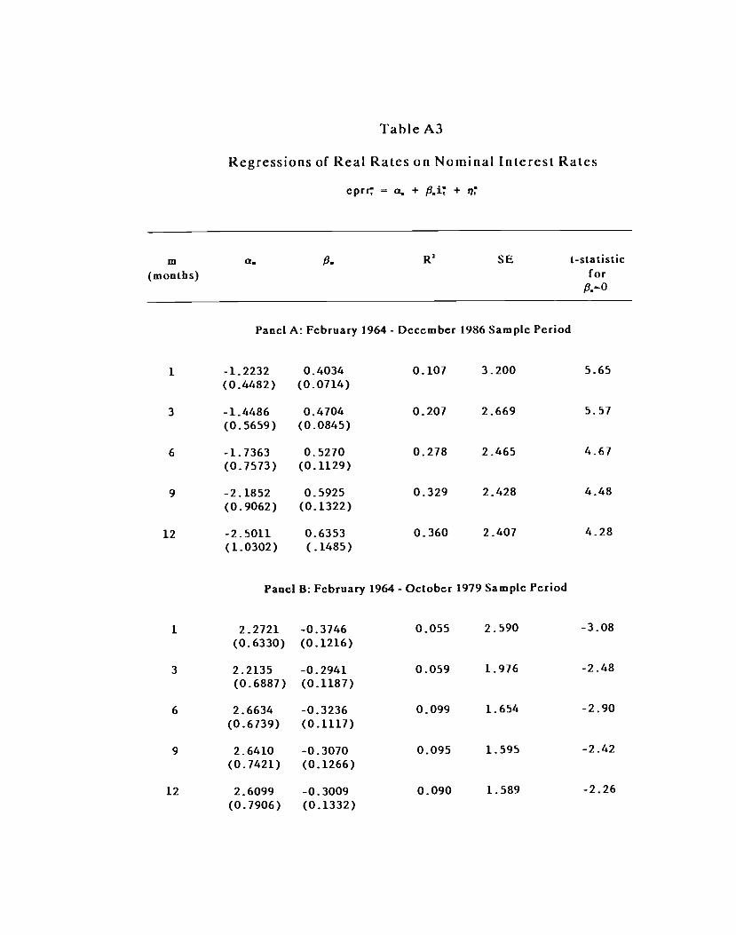
Table A3

Regressions of Real Rates on Nominal Interest Rates

cprr a + + i

m R SE t-statistic(months) for

Panel A: February 1964- December 1986 Sample Period

1 -1.2232 0.4034 0.107 3.200 5.65

(0.4482) (0.0714)

3 -1.4486 0.4704 0.207 2.669 5.51

(0.5659) (0.0845)

6 -1.7363 0.5270 0.278 2.465 4.61

(0.7573) (0.1129)

9 -2.1852 0.5925 0.329 2.428 4.48

(0.9062) (0.1322)

12 -2.5011 0.6353 0.360 2.407 4.28

(1.0302) (.1485)

Panel B: February 1964 - October 1979 Sample Period

1 2.2721 -0.3746 0.055 2.590 -3.08(0.6330) (0.1216)

3 2.2135 -0.2941 0.059 1.976 -2.48

(0.6887) (0.1181)

6 2.6634 -0.3236 0.099 1.654 -2.90

(0.6139) (0.1117)

9 2.6410 -0.3010 0.095 1.595 -2.42(0.7421) (0.1266)

12 2.6099 -0.3009 0.090 1.589 -2.26

(0.7906) (0.1332)

Table A3 Continued

m SE 1-statistic

(months) forfl.=°

Panel C: November 1979- October 1982 Sample I'criod

1 -7.1035 0.9110 0.331 3.498 587(1.8326) (0.1552)

3 -5.0256 0.7647 0.282 2.937 3.03

(3.4120) (0.2526)

6 -7.0521 0.9644 0.384 2.614 3.34

(4.1291) (0.2887)

9 -10.7631 1.2785 0.552 2.382 6.00

(3.3612) (0.2129)

12 -10.6754 1.2918 0.573 2.239 8.25

(2.7065) (0.1567)

Panel D: November 1982 - December 1986 Sample Period

1 1.7349 0.3659 0.040 2.474 1.55

(1.9260) (0.2362)

3 0.1532 0.5946 0.191 1.806 3.11

(1.6798) (0.1910)

6 -1.2817 0.7649 0.470 L301 4.10(1.7622) (0.1867)

9 -1.8158 0.8294 0.605 1.109 4.60

(1.7917) (0.1803)

12 -2.4821 0.9073 0.701 1.017 5.98

(1.5415) (0.1518)

Notcs for Table Al:

Standard errors of coefficients in parentheses.SE = standard error of the regression.

29

correlation of real and noniinal interest rates. These results are consistent

with those found eahier in the literature."

TahIeA4 reportssimilar ex-post real rate regressions. hutwith expected

inflation, E1[irTj, as the explanatory variable. Here the regressions areestimated with the two-step two-stage least squares procedure outlined in

Cumby, Huizinga and Ohstfeld (1983), generating expected inflation using asinstruments the nominal interest rate and two lags of inflation following along

the lines of Huizinga and Mishkin (1986a).34 These results also appear to

strongly reject the constancy of the real rate with large t-statistics on 6m,with

the exception of the post-October 1982 sample period. Furthermore, the a,,,

coefficients are almost always negative suggesting a negative correlationbetween real rates and expected inflation. This negative association of realrates and expected inflation has also been repeatedly found in the literature

for many sample periods."Table A5 and A6 examine whether the high t-statistics inTablesA3 and

A4 really do produce statistically significant rejections of the constancy of the

real rate. The Monte Carlo simulation experiments were conducted asfollows. The data generating process is specified to be one in which the Mr'

and AiT variables are generated from error correction models in which the

parameters were estimated from the relevant sample periods. The ex-postreal rates were generated assuming that the ex-post real rates were serially

uncorrelated, which must he the case under the null hypothesis of constant

"For example, in Mishkin (1981) and Huizinga and Mishkin (1984, 1986).

More specifically, the instruments arc the constant term i", w7.,and The Newey-West(1987) technique is used to ensure positive-definiteness of the variance-covariance matrix ratherthan a spectral method as in Cumby, Huizinga and Obstfeld (1983).

"See for example, Fama and Gibbons (1982), Summers (1983) and Huizinga and Mishkin(1986a).

Table A4

Regressions of Real Rates on Expected Inflation

cprr a + fl.E,[ir + t

m a, SE (-statistic(months) for

fl..O

Panel A: Fcbruary 1964 - Dccember 1986 Sample Period

1 2.1188 -0.3475 0.008 3.372 -4.58(0.3742) (0.0759)

3 3.0886 -0.3609 -0.061 3.087 -3.40

(0.5260) (0.1061)

6 3.4533 -0.4120 -0.073 3.004 -3.19

(0.6746) (01291)

9 3.5984 -0.4375 -0.049 3.037 -2.95

(0.8256) (0.1483)

12 3.4696 -0.4086 -0.052 3.086 -2.29

(1.0225) (0.1788)

Panel B: February 1964 - October 1979 Sample Period

1 2.4463 -0.4301 0.131 2.483 -9.76(0.2226) (0.0441)

3 2.4303 -0.3644 0.131 1.899 -7.24

(0.2781) (0.0503)

6 2.3530 -0.3094 0.185 1.573 -6.44

(0.2821) (0.0481)

9 2.3576 -0.3252 0.117 1.521 -6.35

(0.3122) (0.0512)

12 2.2295 -0.3131 0.127 1.556 -5.57

(0.3517) (0.0562)

Table A4 Continued

m a. . SE 1-statistic(months) for

3.-0

Panel C: November 1979 - October 1982 Sample Period

1 11.5490 -0.9466 0.188 3.873 -5.04

(1.6122) (0.1878)

3 7.7477 -0.3556 0.055 3.370 -1.37

(1.9238) (0.2600)

6 11.4869 -0.8022 0.382 2.679 -3.45

(1.1311) (0.2324)

9 14.4616 -1.2095 0.576 2.318 -8.47

(1.2887) (0.1429)

12 14.0540 -1.1829 0.656 2.009 -1.88

(1.3162) (0.1502)

Panel D: November 1982 - December 1986 Sample Period

1 5.8701 -0.4038 0.068 2.439 -2.06(0.6834) (0.1964)

3 4.8182 0.0155 0.005 2.003 0.12

(2.1181) (0.6249)

6 -1.4169 1.9549 0.289 1.506 0.70

(9.6605) (2.7823)

9 6.6598 -0.3669 -0.056 1.813 -0.51

(2.6150) (0.7203)

12 6.4606 -0.3361 0.016 1.844 -1.91

(0.5918) (0.1760)

Notes for Table A2:

Standard errors of coefficients in parentheses.SE = standard error of the regression.

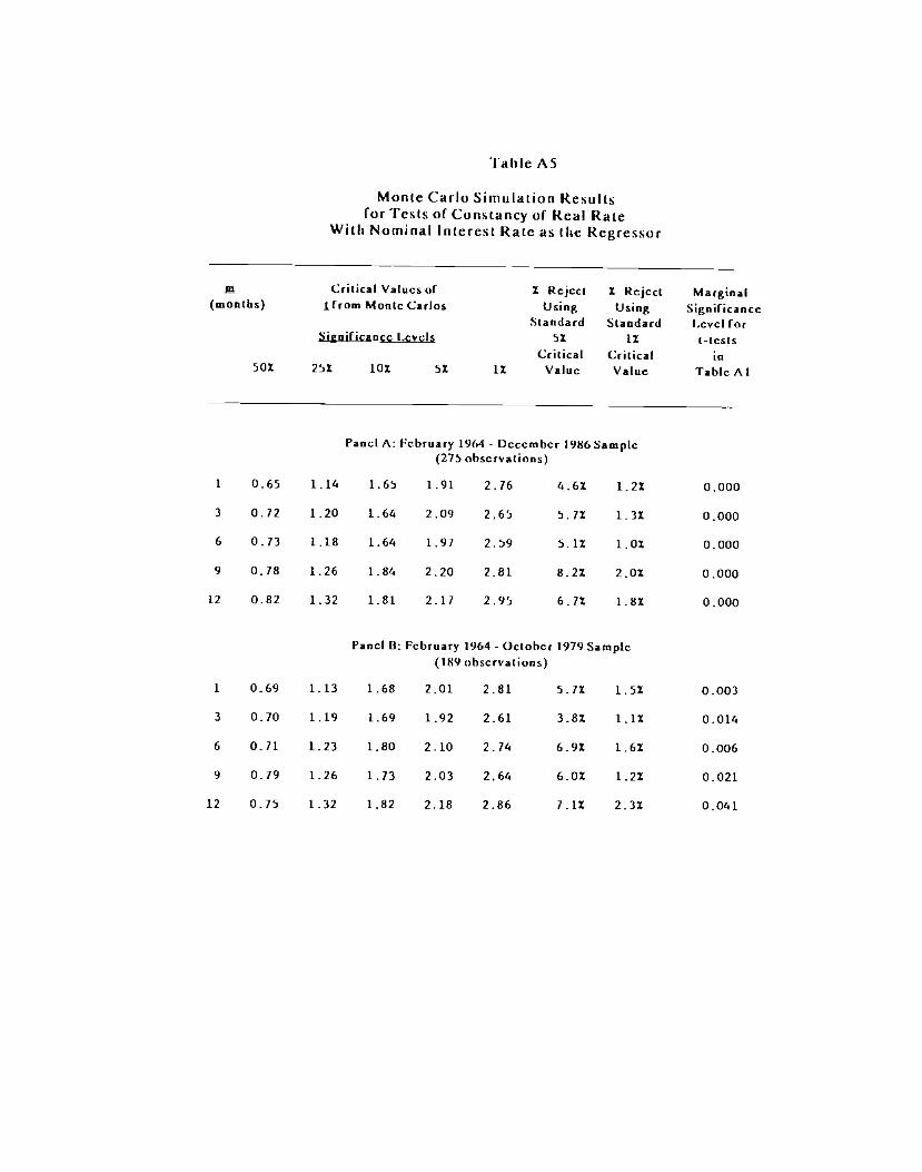
Table AS

Monte Carlo Simulation Resultsfor Tests of Constancy of Real Rate

With Nominal Interest Rate as the Regressor

Critical Values of 1 Reject 1 Rejcc( Marginal(months) Ifrom Monte Carlos Using Using Significancc

Standard Standard Lcvcl forSignificance LcvIt 51 Il (-(cats

Critical Critical in501 251 lox 51 IX Value Value Table Al

Panel A: February 1964- December 1986 Sample(275 observations)

1 0.65 1.14 1.65 1.91 2.76 4.61 1.21 0.000

3 0.72 1.20 1.64 2.09 2.65 5.11 1.31 0.000

6 0.73 1.18 1.64 1.91 2.59 5.11 1.01 0.000

9 0.78 1.26 1.86 2.20 2.81 8.21 2.01 0.000

12 0.82 1.32 1.81 2.1/ 2.95 6.71 1.81 0.000

Panel II: February 964 - October 1979 Sample(189 observations)

1 0.69 1.13 1.68 2.01 2.81 5.11 1.52 0.003

3 0.70 1.19 1.69 1.92 2.61 3.82 1.11 0.014

6 0.71 1.23 1.80 2.10 2./4 6.91 1.62 0.006

9 0./9 1.26 1.73 2.03 2.64 6.02 1.22 0.021

12 0.75 1.32 1.82 2.18 2.86 1.12 2.31 0.041

•I'able A5 Continued

m Critical Values of 2 kcjcct 2 Rcjcct Marginal(months) . from Montc Carlos Using Using Significance

Standard Standard Lcvcl forSini1icancc Lcvcls 52 11 t-csls

Critical Critical in501 251 lOX 52 IX Valuc Value Tabic Al

Panci C: Novcmbcr 1979 -Octobcr 1982 Samplc(36 ohscrvations)

1 0.70 1.23 1.86 2.21 3.01 1.91 2.81 0.000

3 0.81 1.35 1.88 2.27 3.05 8.61 3.11 0.012

6 0.93 1.59 2.23 2.73 3.60 14.21 6.41 0.014

9 0.99 1.60 2.21 2.76 4.17 15.01 6.01 0.002

12 1.10 193 2.87 3.61 5.07 246X 13.91 0.000

Panci D: Novcmbcr 1982- Dcccmbcr 1986 Samplc(50 observations)

1 0.66 1.19 1./8 2.10 2.97 6.82 1.92 0.145

3 0.81 1.25 1.82 2.20 3.19 8.02 2.32 0.011

6 0.80 1.36 1.96 2.24 3.50 10.12 3.31 0.003

9 0.93 1.45 2.09 2.60 3.87 12.02 5.12 0.006

12 1.08 1.69 2.46 3.03 4.10 18.72 8.82 0.002

Table Aô

Monte Carlo Simulation Resultsfor Tests of Constancy of Real Rate

With Eapected Inflation as the Regressor

Critical Values of 1 Rcjcc 1 Rcjcc Marginal(months) Ifrom Monte Carlos Using Using Significance

Standard Standard Lcvcl forSigni(kdnc Jcvcls 52 IX 1-tests

Critical Critical in502 252 lox 12 Value Value Table A2

Panel A: February 1964 - Dcccmbcr 1986 Sampic(275 obscrvations)

1 0.70 1.18 1.65 1.96 2.68 5.02 1.11 0.000

3 0.72 1.21 1.72 2.03 2.55 5.81 0.91 0.000

6 0.69 1.11 1.10 2.00 2.80 5.21 1.41 0.005

9 0.15 1.24 1.79 2.12 2.13 6.61 1.62 0.003

12 0.78 1.33 1.88 2.21 3.0/ 8./2 2.12 0.041

Panel B: February 1964 - October 1979 Sample(189 observations)

1 0./0 1.18 1.61 2.03 2.69 5.72 1.22 0.000

3 0.66 1.14 1.64 1.94 2.60 4.72 1.02 0.000

6 0./2 1.27 1.80 2.18 2.68 7.21 1.52 0.000

9 0.80 1.28 1.19 2.13 2.95 73X 2.32 0.000

12 0.81 1.39 1.91 2.30 2.92 9.21 2.52 0.000

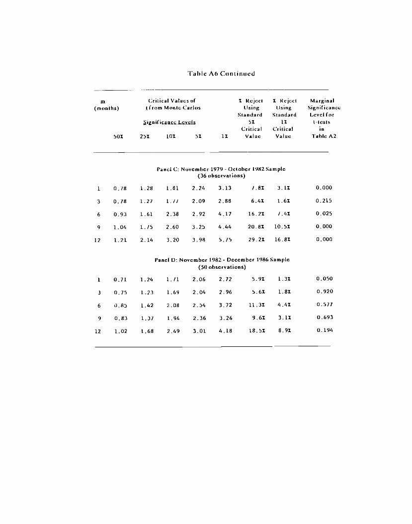
lahic A6 Continued

(2riical Values ol 2 kcjccl 2 Reject Marginal(months) I horn Monic Carlos Using Using Significance

Standard Standard Lcvct forjgni(icancc Levels 52 12 (-(cats

Critical Critical in502 252 102 52 12 Value Value laMe A2

Panci C: November 1979- Octobcr 1982 Samplc(36 ohscrvations)

1 0.78 1.28 1.81 2.24 3.13 7.82 3.12 0.000

3 0.78 1.27 1.11 2.09 2.88 6.42 1.62 0.215

6 0.93 1.61 2.38 2.92 4.17 16.22 L42 0.025

9 1.04 1.75 2.60 3.25 4.44 20.82 10.52 0.000

12 1.21 2.14 3.20 3.98 5./5 29.22 16.82 0.000

Passcl I): Novcmbcr 1982- Dcccmbcr 1986 Samplc(50 observations)

1 0.11 1.24 1.11 2.06 2.72 5.92 1.32 0.050

3 0.75 1.23 1.69 2.04 2.96 5.62 1.82 0.920

6 0.85 1.42 2.08 2.54 3./2 11.32 4.42 0.577

9 0.83 1.37 1.94 2.36 3.26 9.62 3.12 0.693

12 1.02 1.68 2.49 3.01 4.18 18.52 8.92 0.194

30

real rates and rational expectations. The error terms were drawn from anormal distribution in which the variance follows an ARCI-1 process whoseparameters were also estimated from the relevant sample periods. Start up

values were generated with the procedure described earlier in the paper.The results in Table A5 indicate that the nonstationarity of the

regressors has little impact on inference. For the longer sample periods inPanels A and B, the critical values and the percentage rejections using the

usual critical values are very close to those from the standard asymptotic

distributions. With the shortening of the sample period in Panels C and D, the

percentage rejections are higher than that indicated by the asymptoticdistribution and grow with the degree of overlap in the data (i.e., a higher.rn).

However, this phenomenon does not appear to be the result of nonstationarity

of the regressors, hut is rather a small sample problem which appears in other

contexts.36 The last column in Table AS gives the marginal significance levels

for the tests of real rate constancy from the Monte Carlo experiments, and not

surprisingly given the large t-statistics in Table A3, in all but one case the

constancy of real rates is rejected, and usually the rejection is at the 1% level.

Table A6 tells a fairly similar story to Table A5. The constancy of the

real rates is strongly rejected in all but the post-October 1982 sample period -- but even in this period there is one rejection at the 5% significance level (for

in I in Panel D).

The final two tables report on tests of correlation of the real rate with

both nominal rates and expected inflation. Here the constancy of the real rate

is no longer assumed. The interest rate and ex post real rate variables aregenerated with the same procedures as used in Tables AS and A6, except that

ex-post real rates are now allowed to have serial correlation, so that they are

For cxamptc, sec the Monft Carlo simulation rcsults in Mishkin (1990).

31

generated from ARIMA models. In other words, the null now assumes that

inflation and interest rates are contegrated. hut that the real rate is not

constant.

The results in Tables A7 and A8 indicate that allowing real rates to be

serially correlated does have a major impact on the Monte Carlo results. Now

the percentage rejections are much greater than that indicated by the standard

asymptotic distribution. Using a 5% critical value, we sometimes see that the

test statistics reject over fifty percent of the time in Table A7 if the null is true.

The last column in Tables A7 and A8 tell us the statistical significance of the

correlation of real rates with nominal rates and expected inflation, not

assuming constancy of the real rates. The Table A7 marginal significance

levels from the Monte Carlo experiments indicate that there is some evidence

for a positive correlation between nominal and real interest rates in the full

Panel A sample period: we can reject the null of no correlation at the 5% level

in two cases, whenni = 9 and 12 and at the 10% level form = 1 and 3. On the

other hand, the Panel B results cast doubt on the view that real and nominal

rates were significantly negatively correlated in the pre-October 1979 period

because, except for in = 1 when the marginal significance level is 0.069, the

marginal significance levels are quite high despite the apparently large t-statistics in Table A3. The Panel C results, however, do suggest a significant

positive correlation between real and nominal interest rates in the October

1979 to September 1982 period when the Fed altered its operating procedures.

The null of no correlation can he rejected at the five percent level for in = 1

and 12 and the marginal significance levels are fairly low for the other

horizons. The post-October 1982 sample period provides some weak evidence

for a positive correlation of real and nominal rates, because all the marginal

significance levels are near the 10% level although there are no rejections at

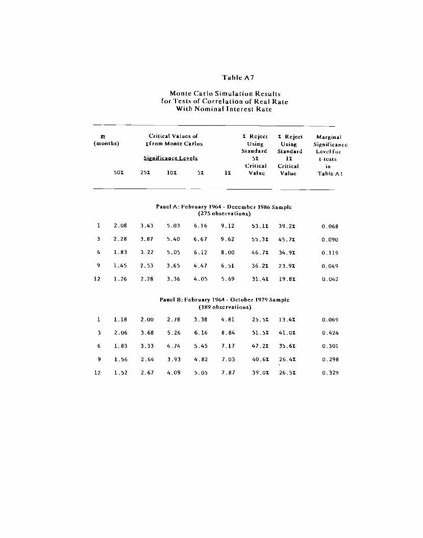
'Fable A7

Monte Carlo Simulation Resultsfor Tests of Correlation of Real Rate

With Nominal Interest Rate

Critical Values of 1 Reject 1 Rcjcct Marginal(months) [from Montc Cartos Using Using Significance

Standard Standard Lcvcl (orSignificancc Lcvcls 51 11 t-tcsls

Critical Critical in501 251 101 51 11 Value Value Table Al

Panel A: February 1964 - Dcccmhcr 1986 Sample(275 obscrvalions)

1 2.08 3.43 5.03 6.16 9.12 53.11 39.21 0.068

3 2.28 3.81 5.40 6.67 9.62 55.31 45.71 0.090

6 1.83 3.22 5.05 6.12 8.00 46.11 34.91 0.119

9 1.45 2.53 3.65 4.41 6.51 36.21 23.91 0.049

12 1.26 2.28 3.36 4.05 5.69 31.41 19.81 0.062

Panel B: February 1964 - October 1979 Samplc(189 observations)

1 1.18 2.00 2.18 3.38 4.81 25.51 13.41 0.069

3 2.06 3.68 5.26 6.16 8.84 51.51 41.01 0.424

6 1.83 3.33 4.14 5.45 1.17 47.21 35.61 0.301

9 1.56 2.64 3.93 4.82 7.03 40.61 26.41 0.298

12 1.52 2.67 4.09 5.05 7.87 39.01 26.51 0.329

lable A7 Continued

Critical Values of 1 Reject I Rcjcc( Marginal(months) I From Monte Carlos Using Using Signilicancc

Standard Standard Level rorigni(icapc LvI 51 Il t-lcsts

Critical Critical in501 251 lOX 51 11 Value Valuc Tabic Al

Panel C: November 1979 - October 1982 Sample(36 obscrvations)

1 1.68 2.94 4.32 5.10 6.71 43.61 31.11 0.028

3 1.12 2.15 3.40 4.17 6.49 28.41 18.01 0.133

6 1.44 2.52 4.01 5.04 8.04 36.61 23.81 0.156

9 1.55 2.95 4.59 6.08 9.24 40.41 29.11 0.054

12 1.75 3.14 5.31 6.45 9.94 44.41 32.51 0.025

Panel 1): November 1982- Dcccmbcr 1986 Sample(SO observations)

1 0.65 1.14 1.61 2.12 2.80 6.71 2.01 0.134

3 1.09 2.02 2.96 3.56 5.48 26.41 14.11 0.085

6 1.46 2.67 4.30 5.37 7.79 39.62 21.01 0.115

9 1.64 3.00 4.49 5.89 9.34 43.11 30.81 0.093

12 1.67 3.30 5.18 6.62 10.67 44.42 34.51 0.061

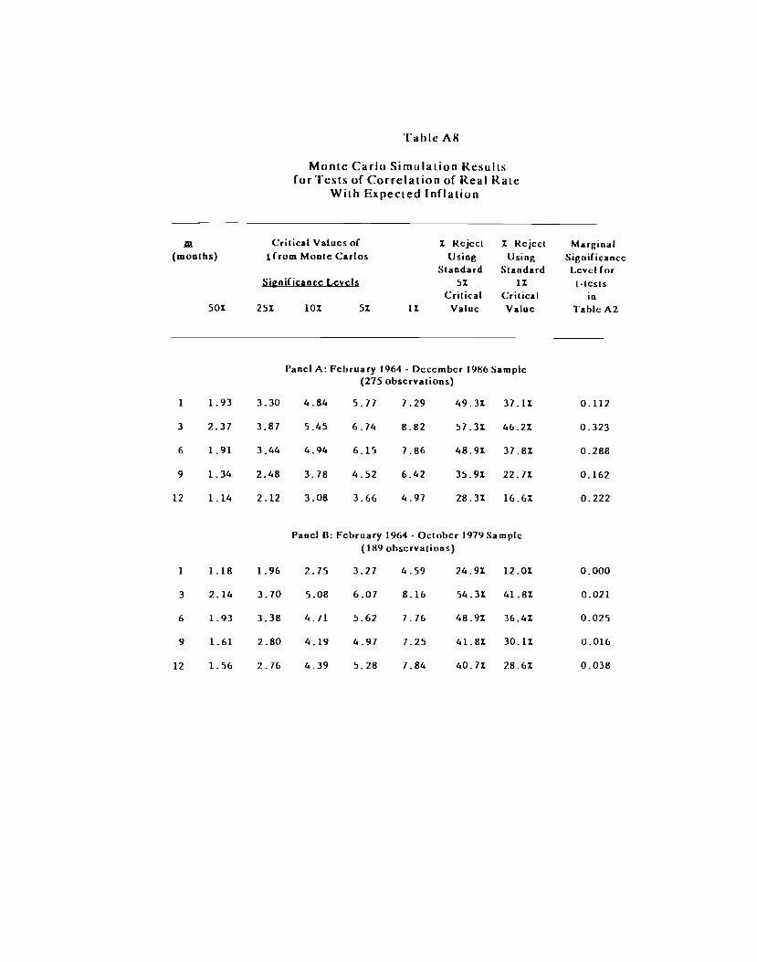
'l'ablc A

Monte Carlo Simulation Resultsfor Tests of Correlation of Real Rate

With Expected Inflation

Critical Values of 2 Reject I Reject Marginal(montks) I from Monte Carlos Using Using Significance

Standard Standard Lcvcl forSigniFicancc Lcycls 52 Ii I-tests

Critical Critical in502 252 102 5% 12 Valuc Valuc Tablc A2

Panel A: February 1964 - Dcccmbcr 1986 Sample(275 observations)

1 1.93 3.30 4.84 5.71 7.29 49.3% 37.12 0.112

3 2.3/ 3.8/ 5.45 6.74 8.82 57.3% 46.22 0.323

6 1.91 3.44 4.94 6.15 7.86 48.92 37.82 0.288

9 1.34 2.48 3.78 4.52 6.42 35.9% 22.72 0.162

12 1.14 2.12 3.08 3.66 4.91 28.32 16.62 0.222

l'aacl B: February 1964 - Octobcr 1979 Samptc(189 observations)

1 1.18 1.96 2./5 3.27 4.59 24.9% 12.0% 0.000

3 2.14 3.70 5.08 6.01 8.16 54.3% 41.82 0.021

6 1.93 3.38 4/1 5.62 7.16 48.9% 36.4% 0.025

9 1.61 2.80 4.19 4.97 7.25 41.82 30.12 0.016

12 1.56 2.76 6.39 5.28 7.84 40.7% 28.6% 0.038

'I'ablc AH (;on(inucd

Critical Values of I Rcjccl 1 Reject Marginal(months) Ifrom Montc Cartos Using Using Signilicancc

Standard Standard Lcvcl forSignificanec Levels SI ii (-tests

Critical Critical in501 251 101 51 1.1 Valuc Valuc Table A2

Panel C: Novcmbcr 1979- Octobcr 1982 Samplc(36 obscrvauons)

1 1.50 2.60 3.61 4.21 5.36 36.41 25.31 0.018

3 1.46 2.55 3.82 6.86 1.79 36.41 24.81 0.531

6 1.91 3.38 5.21 6.51 10.73 48.71 36.41 0.243

9 2.00 3./9 6.36 8.49 13.28 50.11 39./1 0.050

12 2.31 4.02 7.17 9.11 14.13 56z 46.11 0.078

Panel D: Novcmbcr 1982- Dcccmber 1986 Sample

(50 observations)

1 0.80 1.32 1.82 2.23 2.97 8.41 2.41 0.065

3 1.03 1.12 2.43 2.97 4.19 18.71 8.11 0.941

6 1.73 3.08 4.83 6.10 9.29 43.81 32:31 0.769

9 1.43 2.61 4.11 4.98 8.47 38.21 25.11 0.816

12 1.85 3.19 4.90 5.88 9.35 41.81 34.61 0.486

32

the 5% level.

The Table A8 marginal significance levels suggest that the evidence for

a negative association or real interest rates with expected inflation is weaker

than we would expect from the large t-statistics found in the regressions. Only

in the Panel B, pre-October 1979 sample period do we always find rejection of

the null of no correlation between real rates and expected inflation at the five

percent level. We also find two significant rejections of the null of nocorrelation between real rates and expected inflation in the Panel C,

November 1979 to October 1982 sample period. However, we do not find that

the rejections of the null in either the Panel A, full sample period, or in the

Panel D, November 1982 to December 1986 sample period. Overall, Table 2

and 6 indicate that there is evidence for a negative association of real rates

and expected inflation, but that it is not always strong in all the sample

periods.Analyzing the importance of nonstationarity of the regressors to

inference about real interest rate behavior indicates that our views on the

strong rejections of constancy of realm interest rates does hold up to the

scrutiny here. However, we may have to weaken somewhat our views of how

strong the support is for the correlation of real rates with nominal rates and

expected inflation."

'Monte Carlo simulations which examine thc strength of conclusions about whether there wasa shift in the stochastic process of real interest rates in October 1979 and October 1982 have notbeen studied here because this has already been done in Huizinga and Mishkin (1986b). The setup of the experiments there is consistent with the conclusions reached in this paper, becausenominal rates and inflation arc assumed to he non-stationary hut cointegrated of order C1[1,1).The results there provide strong support for the position that shifts in the stochastic process ofreal interest rates did take place with the change of Federal Reserve operating procedures inOctober 1979 and October 1982.

33

References

Barsky. Robert B The Fisher Hypothesis and the Forecastability and Persistence of inflation,'Journal ot' Monetary Economics, (1987).

Camphcll, John Y.. and Mankiw, N. Gregory. "Permanent Income, Current income, andConsumption. Princeton University and Harvard University, mimco. (January 1989).

Clarida, Richard H., and Friedman, Benjamin M., "The Behavior of U.S. Short-Term InterestRates Since October 1979," Journal of Finance 39(1984): 671-682.

Cumby, Robert J., Huizinga, John and Obstfeld, Maurice, "Two-Step, Two-Stage Least SquaresEstimation in Model with Rational Expectations," Journal of Econpmetrics,21: 333-55.

Dickey, David A. and Wayne A. Fuller, "Distribution of the Estimators for Autoregressive TimeScrieswith a Unit Root," Journal of the American Statistical Association 74 (June 1979):427-31

,"Likelihood Ratio Statistics forAutoregressive Time Series witha Unit Root." Econometrica 49 (July 1981): 1057-72

DcJong, David N., John C. Nankervis, N.E. Savin, and Charles H. Whiteman, "Integration VersusTrend-Stationarity in Macroeconomic Time Series," Department of Economics,University of Iowa, Working Paper # 88-27a (December 1988)

Engle, Robert F., 'Autoregressive Conditional Heteroscedasticitywith Estimates of the Varianceof the United Kingdom inflation," Econometrica 50 (July 1982): 987-1007.

, and Clive W. Granger, 'Co-Integration and Error Correction: Representation,Estimation and Testing," Econometrica 55 (1987): 251-76.

Fama, Eugene F., 'Short Term Interest Rates as Predictors of Inflation," American EconomicReview 65 (1975): 269-82.

,"The Information in the Term Structure," Journal of Financial Economics 13(1984):509-528.

,and Gibbons. Michael R., "Inflation, Real Returnsand Capital mavestment,"Jpurnalof Monetary Economics 9 (1982): 297-324.

Fisher, Irving, The Theory of Interest (New York: Macmillan 1930).

Galli, Jordi, "Cointegration and the Fisher Effect: A Note," mimeo., M.I.T. (November 1988)

Grangcr, Clive W., and Paul Newbold, "Spurious Regression in Econometrics," Journal ofEconometrics 2 (1974): 111-120.

Hansen, Lars P., "Large Sample Properties of Generalized Method of Moments Estimators,"

34

Econometrieg 50: 1029-54

, Lars, and Hodrick, Robert, 'Forward Exchange Ratcs as Optimal Predictors ofFuture Spot Rates,' Journal p1 Political Economy 88 (1980): 829-53.

Huizinga, John and Mishkin, Frederic S., 'Inflation and Real Interest Rates on Assets withDifferent Risk Characteristics,' Journal of Finance 39(1984): 699-712.

,'Monetary Policy Regime Shifts and the Unusual Behavior ofReal Interest Rates,' Carnegie-Rochester Conference Series on Public Policy, 24 (Spring1986a): 231-74.

,'HowRobustArc.theRcsults? ARcply,'Carnegie-RochesterConference Series on Public Poticv, 24 (Spring 1986b): 289-302.

Mankiw, N. Gregory and Matthew D. Shapiro, 'Do We Reject Too Often? Small SampleProperties of Tests of Rational Expectations Models,' Economics Letters 20(1986): 139-45.

Mishkin, Frederic S., 'The Real Rate of Interest: An Empirical Investigation,' The Cost andConsequences of Inflation, Carnegie-Rochester Conference Series on Public Policy, 15(1981): 151-200.

,'TheReallnterestRate:AMulti-CountryEmpiricalStudy,'CanadianJournalof Economics 17 (May 1984): 283-311

, 'Understanding Real Interest Rates' American Journal of AgriculturalEconomics 70 (December 1988): 1064.72.

, 'What Does the Term Structure of Interest Rates Tell Us About FutureInflation?' Journal of Monetary Economics (January 1990) forthcoming.

Nelson, Charles R., and Schwert, G. William, 'Short-Term interest Rates as Predictors ofInflation: On Testing the Hypothesis that the Real Rate of Interest is Constant,'American Economic Review, 67 (1977): 478-86.

, and Charles I. Plosser, 'Trends and Random Walks in Macroeconomic TimeSeries,' Journal of Monetary Economics (1982): 129-62.

, and Richard Startz, 'The Distribution of the Instrumental Variables Estimatorand its (-Ratio When the Instrument is a Poor One,' Discussion Paper #88-07, Universityof Washington, (May 1988).

Newey, W. and West Kenneth, 'A Simple, Positive Definite, Heteroskedasdicity and Autocor-relation Consistent Covariance Matrix,' Econometrica 53(1987): 703-708.

Pcrron. Pierre, 'Testing for a Unite Root in a Time Series with a Changing Mean,' Journal ofBusiness and Economic Statistics, 8 (April 1990): 153-162.

35

Phillips. Peter C. B.. 'Understanding Spurious Regressions in Econometrics." Journal 01Economctrics. 33 (December 1986): 311-40.

, Time Series Regression with a Unit Root.' Econometrica 55 (March 1987):277-301.

Rolcy. V. Vance. The Response of Interest Rates to Money Announcements Under AlternativeOperating Procedures and Reserve Retirement Systems,' NBER Working Paper # 1812,1986.

Rose. Andrew K Is the Real Interest Rate Stable?" Journal of Finance 43 (December 1988):1095-1112.

Schwert, G. William, "Effects of Model Specification on Testsfor Unit Roots in MacroeconomicData," Journal of Monetary Economics 20(1987): 73-1-3.

Said. S.E. and Dickcy, D.A., "Testing for Unit Roots in Autoregressive-Moving Average Modelsof Unknown Order," Biometrikg, 71(1984): 599-608.

Stambaugh, Robert F., Bias in Regressionswith Lagged Stochastic Regressors," Graduate Schoolof Business, University of Chicago, January 1986.

Stock, James H. and Mark W. Watson. Variable Trends in Economic Time Series," Journal ofEconomic Perspectives 3 (Summer 1988): 147-174

Summers, Lawrence H .,"The Non-Adjustment of Nominal Interest Rates: A Study of the FisherEffect," in James Tobin (cd.) A Symposium i0 Honor of Arthur Okun (Washington, D.C.:Brookings Institution)

White, Halbert, "A Heteroskedasticity-Consistent Covariance Matrix Estimator and Direct testsfor Hctcroskcdasticity," Econometrica 48(1980): 817-38.