Near-optimal Observation Selection

using Submodular Functions

Andreas Krause

joint work with Carlos Guestrin (CMU)

River monitoring

Want to monitor ecological condition of rivers and lakes Which locations should we observe?

Mixing zone of San Joaquin and Merced rivers7.4

7.67.8

8

Position along transect (m)pH

valu

e

NIMS(B. Kaiser,

UCLA)

Water distribution networks

Pathogens in water can affect thousands (or millions) of people

Currently: Add chlorine to the source and hope for the best

Sensors in pipes could detect pathogens quickly

1 Sensor: $5,000 (just for chlorine) + deployment, mainten. Must be smart about where to place sensors

Battle of the Water Sensor Networks challenge Get model of a metropolitan area water network Simulator of water flow provided by the EPA Competition for best placements

Collaboration with VanBriesen et al (CMU Civil Engineering)

Fundamental question:Observation Selection

Where should we observe to monitor complex phenomena?

Salt concentration / algae biomass Pathogen distribution Temperature and light field California highway traffic Weblog information cascades …

Spatial prediction

Gaussian processes Model many spatial phenomena well [Cressie ’91] Allow to estimate uncertainty in prediction

Want to select observations minimizing uncertainty How do we quantify informativeness / uncertainty?

Horizontal position

pH

valu

e

Observations A µ V

Unobserved Process (one pH value per

location s 2 V)

Prediction at unobservedlocations V\A

Mutual information [Caselton & Zidek ‘84]

Finite set V of possible locations Find A* µ V maximizing mutual information:

A* = argmax MI(A)

Often, observations A are expensive constraints on which sets A we can pick

Entropy ofuninstrumented

locationsafter sensing

Entropy ofuninstrumented

locationsbefore sensing

Constraints for observation selection

maxA MI(A) subject to some constraints on A What kind of constraints do we consider?

Want to place at most k sensors: |A| · k or: more complex constraints:

All these problems NP hard. Can only hope for approximation guarantees!

Sensors need to communicate (form a tree)Multiple robots(collection of

paths)

Want to find: A* = argmax|A|=k MI(A) Greedy algorithm:

Start with A = ; For i = 1 to k

s* := argmaxs MI(A [ {s}) A := A [ {s*}

Problem is NP hard! How well can this simple heuristic do?

The greedy algorithm

Performance of greedy

Greedy empirically close to optimal. Why?

Greedy

Optimal

SERVER

LAB

KITCHEN

COPYELEC

PHONEQUIET

STORAGE

CONFERENCE

OFFICEOFFICE50

51

52 53

54

46

48

49

47

43

45

44

42 41

3739

38 36

33

3

6

10

11

12

13 14

1516

17

19

2021

22

242526283032

31

2729

23

18

9

5

8

7

4

34

1

2

3540

Temperature datafrom sensor network

S1S2

S3

S4S5

Placement B = {S1,…, S5}

Key observation: Diminishing returns

S1S2

Placement A = {S1, S2}

Theorem [UAI 2005, M. Narasimhan, J. Bilmes]

Mutual information is submodular:For A µ B, MI(A [ {S’}) – MI(A) ¸ MI(B [ {S’})- MI(B)

Adding S’ will help a lot! Adding S’ doesn’t help much

S‘

New sensor S’

Cardinality constraintsTheorem [ICML 2005, with Carlos Guestrin, Ajit Singh]

Greedy MI algorithm provides constant factor approximation: placing k sensors, 8 >0:

Optimalsolution

Result ofgreedy algorithm

Constant factor,~63%

Proof invokes fundamental result by Nemhauser et al ’78 on greedy algorithm for submodular functions

Myopic vs. Nonmyopic Approaches to observation selection

Myopic: Only plan ahead on the next observation Nonmyopic: Look for best set of observations

For finding best k observations, myopic greedy algorithm gives near-optimal nonmyopic results!

What about more complex constraints? Communication constraints Path constraints …

Communication constraints:Wireless sensor placements should

… be very informative (high mutual information) Low uncertainty at unobserved locations

… have low communication cost Minimize the energy spent for communication

SERVER

LAB

KITCHEN

COPYELEC

PHONEQUIET

STORAGE

CONFERENCE

OFFICEOFFICE50

51

52 53

54

46

48

49

47

43

45

44

42 41

3739

38 36

33

3

6

10

11

12

13 14

1516

17

19

2021

22

242526283032

31

2729

23

18

9

5

8

7

4

34

1

2

3540

1.2

1.4

2.11.6

1.9

Communication cost= expected number

of transmissions

SERVER

LAB

KITCHEN

COPYELEC

PHONEQUIET

STORAGE

CONFERENCE

OFFICEOFFICE50

51

52 53

54

46

48

49

47

43

45

44

42 41

3739

38 36

33

3

6

10

11

12

13 14

1516

17

19

2021

22

242526283032

31

2729

23

18

9

5

8

7

4

34

1

2

3540

SERVER

LAB

KITCHEN

COPYELEC

PHONEQUIET

STORAGE

CONFERENCE

OFFICEOFFICE50

51

52 53

54

46

48

49

47

43

45

44

42 41

3739

38 36

33

3

6

10

11

12

13 14

1516

17

19

2021

22

242526283032

31

2729

23

18

9

5

8

7

4

34

1

2

3540

Naive, myopic approach: Greedy-connect

Simple heuristic: Greedily optimize information Then connect nodes to minimize

communication cost

Greedy-Connect can select sensors far apart…Want to find optimal tradeoffbetween information and communication cost

relay node

relay node

Secondmost informative

No communicationpossible!

SERVER

LAB

KITCHEN

COPYELEC

PHONEQUIET

STORAGE

CONFERENCE

OFFICEOFFICE50

51

52 53

54

46

48

49

47

43

45

44

42 41

3739

38 36

33

3

6

10

11

12

13 14

1516

17

19

2021

22

242526283032

31

2729

23

18

9

5

8

7

4

34

1

2

3540

Most informative

efficientcommunication!

Not veryinformative

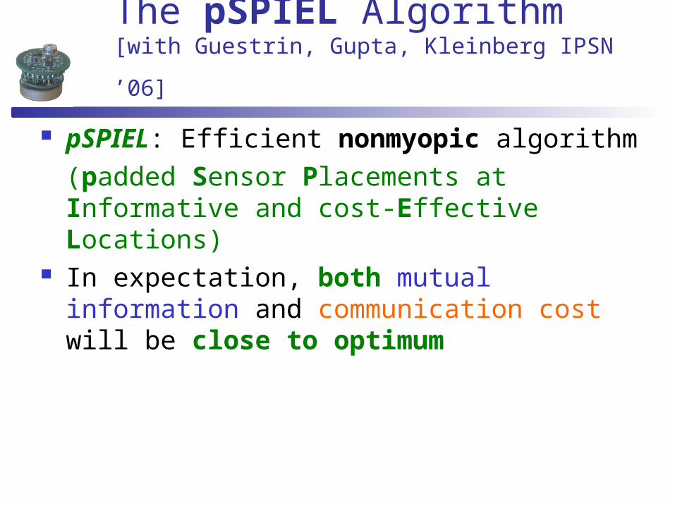
The pSPIEL Algorithm [with Guestrin, Gupta, Kleinberg IPSN ’06]

pSPIEL: Efficient nonmyopic algorithm(padded Sensor Placements at Informative and cost-Effective Locations)

In expectation, both mutual information and communication cost will be close to optimum

Our approach: pSPIEL Decompose sensing region into small, well-

separated clusters Solve cardinality constrained problem per

cluster Combine solutions using k-MST algorithm

C1 C2

C3C41

13

2

1

3 2

21 2

Theorem: pSPIEL finds a tree T with

mutual information MI(T) ¸ () OPTMI,

communication cost C(T) · O(log |V|) OPTcost

[IPSN’06, with Carlos Guestrin, Anupam Gupta, Jon Kleinberg]

Guarantees for pSPIEL

Prototype implementation

Implemented on Tmote Sky motes from MoteIV

Collect measurement and link information and send to base station

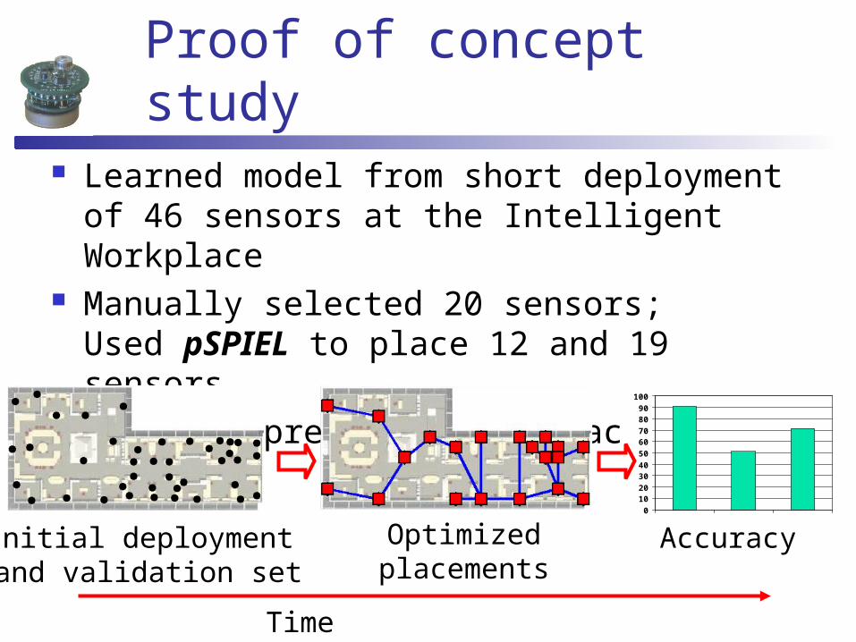
Proof of concept study Learned model from short deployment of

46 sensors at the Intelligent Workplace Manually selected 20 sensors;

Used pSPIEL to place 12 and 19 sensors Compared prediction accuracy

Initial deployment and validation set

Optimizedplacements

0102030405060708090

100

Accuracy

Time

0102030405060708090

100

M20 pS19 pS12

Root mean squares error (Lux)

Proof of concept study

Manual (M20) pSPIEL (pS19) pSPIEL (pS12)

0102030405060708090

100

M20 pS19 pS12

Root mean squares error (Lux)

0102030405060708090

100

M20 pS19 pS12

Root mean squares error (Lux)

0

5

10

15

20

25

30

M20 pS19 pS12

0

5

10

15

20

25

30

M20 pS19 pS12

0

5

10

15

20

25

30

M20 pS19 pS12

Communication cost (ETX)

bett

er

bett

er

Path constraints

Want to plan informative paths Find collection of paths P1,…,Pk s.t.

MI(P1 [ … [ Pk) is maximized Length(Pi) · B

Path ofRobot-1

Path ofRobot-2Path of

Robot-3

Start 1

Start 3

Start 2

Outline ofLake Fulmor

Naïve, myopic algorithm

Go to most informative reachable observations Again, the naïve myopic approach can fail badly!

Looking at benefit cost-ratio doesn’t help either Can get nonmyopic approximation algorithm

[with Amarjeet Singh, Carlos Guestrin, William Kaiser, IJCAI 07]

Start 1Most informativeobservation

Waste (almost)all fuel!Have to go back

without furtherobservations

Comparison with heuristic

Approximation algorithm outperforms state-of-the-art heuristic for orienteering

4

6

8

10

12

14

200 250 300 350 400 450Cost of output path (meters)

Submodularpath planning

Known heuristic [Chao et. al’ 96]

More

info

rmati

ve

Submodular observation selection

Many other submodular objectives (other than MI) Variance reduction: F(A) = Var(Y) – Var(Y | A) (Geometric) coverage: F(A) = |area covered| Influence in social networks (viral marketing) Size of information cascades in blog networks …

Key underlying problem:Constrained maximization of submodular functions

Our algorithms work for any submodular function!

Water Networks 12,527 junctions 3.6 million contamination

events

Place 20 sensors to Maximize detection likelihood Minimize detection time Minimize population affected

Theorem:All these objectives are submodular!

0 5 10 15 200

0.2

0.4

0.6

0.8

1

1.2

1.4

Number of sensors

Pop

ulat

ion

affe

cted

Greedysolution

0 5 10 15 200

0.2

0.4

0.6

0.8

1

1.2

1.4

Number of sensors

Pop

ulat

ion

affe

cted

Greedysolution

offline bound

Bounds on optimal solution

Submodularity gives online bounds on the performance of any algorithm

0 5 10 15 200

0.2

0.4

0.6

0.8

1

1.2

1.4

Number of sensors

Pop

ulat

ion

affe

cted

Greedysolution

online bound

offline bound

Pen

alt

y r

ed

uct

ion

Hig

her

is b

ett

er

Results of BWSN [Ostfeld et al]

Author #non-dom.(out of 30)

Krause et. al. 26

Berry et. al. 21

Dorini et. al. 20

Wu and Walski 19

Ostfeld and Salomons 14

Propato and Piller 12

Eliades and Polycarpou

11

Huang et. al. 7

Guan et. al. 4

Ghimire and Barkdoll 3

Trachtman 2

Gueli 2

Preis and Ostfeld 1

Multi-criterion optimization

[Ostfeld et al ‘07]: count number of non-dominated solutions

Conclusions Observation selection is an important AI

problem Key algorithmic problem: Constrained

maximization of submodular functions For budgeted placements, greedy is near-

optimal! For more complex constraints (paths, etc.):

Myopic (greedy) algorithms fail presented near-optimal nonmyopic algorithms

Algorithms perform well on several real-world

observation selection problemsSERVER

LAB

KITCHEN

COPYELEC

PHONEQUIET

STORAGE

CONFERENCE

OFFICEOFFICE50

51

52 53

54

46

48

49

47

43

45

44

42 41

3739

38 36

33

3

6

10

11

12

13 14

1516

17

19

2021

22

242526283032

31

2729

23

18

9

5

8

7

4

34

1

2

3540