near-rational wage and price setting and the long-run

Near-Rational Wage and Price Setting and the Long-Run Phillips Curve

OVER THIRTY YEARS ago, in his presidential address to the American Eco-nomic Association, Milton Friedman asserted that in the long run thePhillips curve was vertical at a natural rate of unemployment that couldbe identified by the behavior of inflation.1 Unemployment below thenatural rate would generate accelerating inflation, and unemploymentabove it, accelerating deflation. Five years later the New Classical econo-mists posed a further challenge to the stabilization orthodoxy of the day. Intheir models with rational expectations, not only was monetary policyunable to alter the long-term level of unemployment, it could not even con-tribute to stabilization around the natural rate.2 The New Keynesianeconomics has shown that, even with rational expectations, small amountsof wage and price stickiness permit a stabilizing monetary policy.3 But

1

G E O R G E A . A K E R L O FUniversity of California, Berkeley

W I L L I A M T. D I C K E N SBrookings Institution

G E O R G E L . P E R R YBrookings Institution

The authors would like to thank Peter Kimball, Kathleen Withers, Marc-Andreas Muendler,and Megan Monroe for invaluable research assistance. We also thank Zarina Durrani for herpatient instruction in how compensation professionals make decisions and how they takeinflation into account. The authors wish to thank Robert Akerlof, Pierre Fortin, David Levine,Maurice Obstfeld, David Romer, Robert Solow, and participants in seminars at Williams Col-lege, Georgetown University, the University of California at Berkeley, the Levy Institute, andthe Bank of Canada for valuable comments. George Akerlof is grateful to the Canadian Insti-tute for Advanced Research, the MacArthur Foundation, and the Brookings Institution forfinancial support. William Dickens and George Akerlof also wish to thank the National ScienceFoundation for financial support under research grant number SBR 97-09250.

1. Friedman (1968); see also Phelps (1968) for an analysis very similar to that of Friedman.2. See, for example, Lucas (1972); Sargent (1973).3. See Akerlof and Yellen (1985); Mankiw (1985).

9573—02 BPEA Akerlo/Dickens/Per 7/21/00 10:18

the idea of a natural unemployment rate that is invariant to inflation stillcharacterizes macroeconomic modeling and informs policymaking.

The familiar empirical counterpart to the theoretical natural rate is thenonaccelerating-inflation rate of unemployment, or NAIRU. Phillipscurves embodying a NAIRU are estimated using lagged inflation as aproxy for inflationary expectations. NAIRU models appear in most text-books, and estimates of the NAIRU—which is assumed to be relativelyconstant—are widely used by economic forecasters, policy analysts, andpolicymakers. However, the inadequacy of such models has been demon-strated forcefully in recent years, as low and stable rates of inflation havecoexisted with a wide range of unemployment rates. If there were a single,relatively constant natural rate, we should have seen inflation slowingsignificantly when unemployment was above that rate, and rising when itwas below. Instead, the inflation rate has remained fairly steady, withannual inflation as measured by the urban consumer price index (CPI-U)ranging from 1.6 to 3.0 percent since 1992, while the unemployment ratehas ranged from 6.8 to 3.9 percent. In this paper we present a model thatcan accommodate relatively constant inflation over a wide range of unem-ployment rates.

Another motivation is a recent finding by William Brainard and GeorgePerry.4 Estimating a Phillips curve in which all the parameters are allowedto vary over time, they find that the coefficient on the proxy for expectedinflation in the Phillips curve has changed considerably, while otherparameters of that model have been relatively constant. In particular,Brainard and Perry found that the coefficient on expected inflation wasinitially low in the 1950s and 1960s, grew in the 1970s, and has fallensince then. The model we present can explain both why the coefficient onexpected inflation might be expected to change over time and, to someextent, the time pattern of changes observed by Brainard and Perry.

Our paper also allows an interpretation of the findings of Robert Kingand Mark Watson and of Ray Fair.5 Both find a long-run trade-off betweeninflation and unemployment. In addition, King and Watson find that theamount of inflation that must be tolerated to obtain a given reduction ofunemployment rose considerably after 1970. Our model allows a trade-off,but only at low rates of inflation such as those that prevailed in the 1950s,

2 Brookings Papers on Economic Activity, 1:2000

4. Brainard and Perry (2000).5. King and Watson (1994); Fair (2000).


1960s, and 1990s. At higher rates of inflation, the trade-off is reduced, andat high enough rates of inflation, it disappears.

Much of the empirical controversy surrounding the relationshipbetween inflation and unemployment has focused on how people formexpectations. This may be neither the most important theoretical nor themost important empirical issue. Instead, this paper suggests that it is nothow people form expectations but how they use them—and even whetherthey use them at all—that is the issue. Economists typically assume thateconomic agents make the best possible use of the information available tothem. But psychologists who study how people make decisions have adifferent view. They see individuals as acting like intuitive scientists, whobase their decisions on simplified, abstract models.6 However, these simpleintuitive models can be misleading; indeed, sometimes they are incorrect.Psychologists have studied the use of these simplified abstractions, oftencalled mental frames or decision heuristics, and the mistakes that resultfrom them. Economists should not assume absence of cognitive error ineconomic decisions, nor should they assume that their own models andthose of the public exactly coincide.

We propose that there are three important ways in which the treatmentof inflation by real-world economic agents diverges from the treatmentassumed in economic models. First, when inflation is low, a significantnumber of people may ignore inflation when setting wages and prices.Second, even when they take inflation into account, they may not treat it aseconomists assume. In particular, we hypothesize that the informal use ofinflationary expectations in wage and price decisions leads to less thancomplete projection of anticipated inflation, with consequences for theaggregate relation between inflation and unemployment. Finally, webelieve that workers have a different view of inflation from that of trainedeconomists. Workers see inflation as increasing prices and reducing theirreal earnings; they do not fully, if at all, appreciate that inflation increasesthe nominal demand for their services. Thus they tend to view the nomi-nal wage increases they receive at low rates of inflation as a sign that theirwork is appreciated, and to be happier in their jobs as a result. They mayalso be unaware of the extent to which inflation is increasing the pay avail-able to them in alternative jobs. Even fully rational employers, who mustsolve the typical efficiency wage problem, can exploit workers’ misper-

George A. Akerlof, William T. Dickens, and George L. Perry 3

6. See Nisbett and Ross (1980).


ceptions by paying wages that are less than what would be required ifworkers fully incorporated inflation into their mental frames.

If any of these three departures from the fully rational use of informa-tion about inflation are important, then at low rates of inflation, prices andwages will be set consistently lower relative to nominal aggregate demandthan they would be at zero inflation. As a result, operating the macroecon-omy with a low but positive rate of inflation will permit a higher level ofemployment to be sustained. We will show that at low rates of inflation thebehaviors that we posit, which depart from the fully rational decisions oftypical economic models, impose very small costs on those who practicethem. Because there may be subjective or objective costs associated withfully rational behavior, or because implementing fully rational behaviormay require overcoming some perception threshold or behavioral inertia, itis plausible that the costs of nonrational behavior may be too small to inducerational behavior from all economic agents. However, if inflation increases,the costs of being less than perfectly rational about it will also rise, and peo-ple will switch their behavior to take inflation into full account. Thus,although increasing inflation modestly above zero will permit lower unem-ployment, there is a rate of inflation above which the sustainable unem-ployment rate rises as more and more people adopt fully rational behavior.This rate of inflation thus minimizes the sustainable rate of unemployment.

The remainder of the paper proceeds in three steps. First, we describedepartures from perfect rationality at low rates of inflation and presentsome evidence that supports our view. Second, we formally derive ourmodel of near-rational wage and price setting, show that the costs of nearrationality are small, derive short- and long-run Phillips curves from themodel, and present a calibration exercise that shows that, even when onlya fraction of wages and prices are influenced by near-rational behavior,there can still be substantial long-run gains in employment from moderate,rather than very low or zero, inflation. Finally, we estimate the theoreticalmodel using postwar quarterly U.S. data. The results support the theoreti-cal model and are surprisingly robust.

Near-Rational Behavior Toward Inflation

As noted above, psychologists who study decisionmaking approach itdifferently from the way economists do. Psychologists have identified



many ways in which real-world decisionmaking departs from economicrationality. Here we describe three ways in which we suspect that behaviortoward inflation departs from the economist’s rational model.

First, psychologists suggest that decisionmakers, far from making thebest use of available information, readily ignore potentially relevantconsiderations and discard potentially relevant information in order tosimplify their decision problems. Daniel Kahneman and Amos Tverskyhave dubbed this behavior editing.7 When people “edit” decision problems,they rule out less important considerations in order to concentrate on thefew factors that matter most. In this regard, real-world decisionmakers areno different from academic economists when they construct models: unim-portant factors are ignored in order to concentrate on important factors. Arelated literature in the psychology of perception suggests that items mustreach a threshold of salience before they are even perceived.8 Thus, wheninflation is low, it may be at most a marginal factor in wage and price deci-sions, and decisionmakers may ignore it entirely.9

We know of no strong evidence either for or against the view that somewage and price setters ignore inflation,10 but several before us have sug-gested the occurrence of such behavior. For example, Otto Eckstein and


7. Kahneman and Tversky (1979). Kunreuther (1978) has used the phenomenon of edit-ing to explain why many people do not buy disaster insurance: very low probability eventsare ignored in decisionmaking. His book (pp. 165–86) presents the results of experimentsthat demonstrate the phenomenon of editing.

8. See Gleitman (1996).9. The behavior of cost-of-living-adjustment (COLA) clauses is consistent with increas-

ing attention being paid to inflation at higher levels of inflation. As inflation rose in the1970s and 1980s, coverage of union workers by COLAs in the United States increased. Inthe late 1960s about one-quarter of workers involved in collective bargaining were coveredby COLA clauses, compared with about 60 percent for the inflationary decade from 1975to 1985 (Hendricks and Kahn, 1985, pp. 36–37). As inflation fell in the late 1980s, thefraction covered fell to 40 percent in 1990 (Holland, 1995, p. 176). Such inflation sensitiv-ity of COLAs is consistent with our basic idea that wage and price setters tend to ignoreinflation in their wage and price setting when inflation is low, but tend to take it into accountas inflation rises. But this evidence has at least two other possible explanations. It is wellknown (see Ball, Mankiw, and Romer, 1988, p. 56) that the variance of inflation increaseswith its level. COLAs may increase at higher levels of inflation as insurance against thisvariance. Furthermore, if at higher rates of inflation a greater fraction of inflation is due tomonetary rather than to real shocks, more contracts will be indexed at higher than at lowerrates of inflation (see Gray, 1978).

10. Direct attempts to assess the effects of forecast inflation on wage setting have ignoredthe indirect effects of inflation through other information that will be correlated with infla-tion. Such information includes the wages and prices of competitive and complementary


Roger Brinner based their model of a shifting Phillips curve on the assump-tion that inflationary expectations mattered more in determining inflation inthe 1970s than in the 1960s.11 One major macroeconomics textbookdescribes the postwar U.S. Phillips curve in terms of an early period oflow inflation, which was ignored by wage and price setters, and a laterperiod of high inflation, when the coefficient on the last period’s inflationwas close to one.12 Two of the officials who over the past five years havebeen most responsible for achieving the Federal Reserve’s goal of price sta-bility have also suggested the possibility of inflation editing. Former FedVice Chairman Alan Blinder, in company with coauthors, has theorized:

A businessman who cannot keep infinite amounts of information in his headmay worry about a few important things and ignore the rest. And when nation-wide inflation is low, it may be a good candidate for being ignored. Indeed, oneprominent definition of “price stability” is inflation so low that it ceases to be afactor in influencing decisions.13

Senate testimony of Federal Reserve Chairman Alan Greenspan seemsalso to suggest the view that, at low rates of inflation, economic agentsmay simply ignore it:


goods and factors. Thus the findings that wage and price setters seem to put little weighton inflation (Blinder and others, 1998; Levine, 1993) are inconclusive. For this reason wemade our own attempt to solicit such information. We sent an e-mail questionnaire to ran-domly selected members of the American Compensation Association asking them to rec-ommend wage and salary increases in hypothetical situations varying by respondent in anumber of different dimensions. The respondents were given the type of information thatpersonnel executives typically use to make recommendations for wage and salary changes.This information included the wage and salary increases of other firms in their labor mar-ket over the past year, the desired relative wage and salary position of their firm, expectedwage and salary increases of other firms in their labor market for the next year, the increasein the CPI, the difficulty of hiring and retention, and their firm’s expected net revenue growthrelative to that of its industry and relative to that of the economy as a whole. The mean ofexpected wage increases by other firms in the sample was increased one-for-one with therate of inflation. The total effect of changes in inflation on wage and salary increases by indi-vidual firms can be seen by regressing the recommended wage and salary increases on theexpected wage and salary increases of others and the CPI. The point estimate of the changecaused by a one-point change in the CPI in the wages of an individual firm, given that thatfirm’s changes are representative of other firms facing the same increase in the CPI, is 0.738.This estimate is obtained by dividing the coefficient on the CPI by one minus the coefficienton the expected wage increases of other firms. Unfortunately, this estimate has a very highstandard error, and we cannot rule out the possibility that the impact of an increase inexpected CPI inflation on wage inflation would be one for one, but the point estimate is sug-gestive of our view.

11. Eckstein and Brinner (1972).12. Blanchard (1999, pp. 153–54).13. Blinder and others (1998, p. 98).


By price stability I mean a situation in which households and businesses in mak-ing their savings and investment decisions can safely ignore the possibility ofsustained, generalized price increases or decreases.14

Second, even when people do pay attention to inflation, they may notuse expectations in the way economists typically assume. If economicagents used a formal procedure to make wage and price decisions, theywould first use available information to determine a desired real wage orprice change. They would then add in the amount of inflation they expectbetween the time they are making the decision and some future timeduring the period over which they expect the price or wage to be in effect.But if they make the decisions intuitively, subjectively considering a num-ber of factors simultaneously, including inflation, there is no reason toexpect that the decision will give the appropriate weight to inflation. Onedecision heuristic, suggested to us by interviews with compensationprofessionals, is that information on inflation may simply be averagedalong with other factors to arrive at a nominal wage or price increase.This would mean that an increase in inflation would lead to the setting ofa higher wage or price, but the effect would be less than one for one. Thus,less than complete weighting of inflation is the second departure fromfull rationality that may influence the relationship between inflation andunemployment.

In fact, textbooks for compensation professionals warn against usingthe formal procedure that economists would imagine to be standard. Forexample, George Milkovich and Jerry Newman discourage their readersfrom granting automatic wage and salary increases, including increases forthe cost of living.15 Such automatic grants, these authors say, reduce thefunds available to reward employees for performance. Similar thoughts areexpressed in the handbook of the influential Hay Group of compensationconsultants, in which managers are advised to “avoid linking salary move-ment to changes in the cost of living, because this creates entitlement andreduces the amount of money available to differentiate for performance.”16

The third important departure from the hyperrational model comes fromthe way workers perceive inflation. Robert Shiller has documented verylarge differences between the intuitive models of inflation used by the laypublic, most of whom are wage and salary recipients, and the mental


14. Greenspan (1988, p. 611).15. Milkovich and Newman (1984).16. Rock and Berger (1991, p. 556).


accounting of economists who study the effects of inflation scientifically.17

Wage and salary earners systematically underestimate the effects of infla-tion on the wages that their employers will want to pay them, even in ques-tionnaires where the effects of inflation are quite explicit, so that it ishighly unlikely that inflation is ignored. As a consequence, and especiallyat moderate rates of inflation when real wages are not perceptibly eroded,workers’ job satisfaction may be enhanced by nominal wage increaseseven if they fail to fully reflect inflation.

There is considerable evidence for this sort of reaction on the part ofworkers. Economists see inflation as induced by changes in the moneysupply and thus as having a uniform effect on nominal wages and otherprices, so that inflation causes no change in real income. In his question-naire study, Shiller has shown that, in contrast, the public has no suchexpectations. For example, when asked “to imagine how things would bedifferent if the United States had experienced higher inflation over thelast five years,”18 only 31 percent of his noneconomist subjects believedthat their own nominal income would have been higher than in the absenceof inflation. When asked “to evaluate [a variety] of theories about [how]the effects of general inflation on wages and salary relates to your ownexperience and your own job,” 60 percent of economists, but only 11 per-cent of the general public, elected that “competition among employers willcause my pay to be bid up. I could get outside offers from other employers,and so, to keep me my employer will have to raise my pay too.” A popu-lar answer for the general public (26 percent), in contrast to economists(4 percent), was the following: “the price increase will create extra profitsfor my employer who can now sell output for more; there will be no effecton my pay.”19

These responses suggest that the public fails to understand inflation asa general-equilibrium phenomenon. They believe that inflation will makethem poorer because it bids up the prices of the goods they consume, butthey fail to appreciate fully, if at all, that inflation will also bid up the pricesof other competing factors and other competing workers, thereby resultingin a rise in their own wages and salaries. Thus, according to Shiller, the“biggest gripe about inflation,” expressed by 77 percent of the general


17. Shiller (1997).18. Shiller (1997, p. 21).19. Shiller (1997, pp. 31–32).


public (but only 12 percent of economists), was that inflation “hurts myreal buying power. It makes me poorer.”20

Economists should not be surprised that laypeople underestimate theeffect of inflation on the demand for their own services. One of the mostsignificant differences between trained economists and the lay public iseconomists’ greater appreciation of general equilibrium. The cognitivedifficulty of general equilibrium has been indicated by the fact, noted bythe Commission on Graduate Education, that even economics graduatestudents do not give the correct explanation for why barbers’ wages, inthe technically stagnant hair-cutting industry, have risen over the pastcentury.21 If economics graduate students fail to appreciate the effects onbarbers’ opportunity costs from wage increases due to productivity changeoutside the hair-cutting industry, it would be a stretch to expect the laypublic to see that, as inflation rises, the demand for their services (in nom-inal dollars) will similarly rise with it.

Findings by Eldar Shafir, Peter Diamond, and Tversky are consistentwith those of Shiller. In one vignette, which they related to respondents,these authors draw a contrast between Ann, who receives a 2 percent nom-inal salary increase at zero inflation, and Barbara, who gets a 5 percentnominal salary increase at 4 percent inflation. Most respondents correctlyanswered that Ann would be better off economically,22 but they also saidthat Barbara would be happier and less likely to leave her job. This reac-tion to the vignette suggests that respondents have not ignored the infla-tion, as they would with editing—otherwise Ann would not be judgedbetter off economically. But the other answer, favoring Barbara, suggeststhat they may also underestimate the effect that inflation will have on Bar-bara’s other alternatives, thus leading them to conclude that she will behappier and less likely to quit her job.

Unfortunately, these authors did not probe the reasons why their respon-dents believed Barbara should be happier than Ann, but they are respond-ing as if the inflation has not increased Barbara’s alternatives by an equalamount. If the wages that she could get on the outside, as well as all ofthe prices that she would be paying, have increased by 4 percent, Barbarashould be less happy than Ann and more likely to leave her job. Our modelof inflation, however, suggests a good reason why Barbara should feel hap-


20. Shiller (1997, p. 29).21. Krueger and others (1991, p. 1044).22. Shafir, Diamond, and Tversky (1997).


pier than Ann does and be less likely to quit her job: she does not feelthat her alternatives improve at the rate of inflation. Another question byShiller suggests that the responses obtained to this vignette reflect thetrue opinion of the American public. He finds that about half of the U.S.general public—but only 8 percent of economists—think that they wouldfeel more job satisfaction “if their pay went up . . . even if prices went upas much.”23

Neither the vignette by Shafir and others nor Shiller’s question dealswith the possibility, perhaps on the mind of the public, that the inflationis caused by a supply shock that decreases the real demand for workersrather than a money-neutral demand shock that leaves all demandsunchanged in real terms. Of course, if that is really what is on the mind ofthe public, even when there is a persistent demand-induced increase inthe rate of inflation, workers will still have greater job satisfaction withsome small amount of inflation than with no inflation. This, then, is thethird way in which we think that near rationality may impact the relationbetween inflation and unemployment. If higher job satisfaction at low ratesof inflation leads to higher morale, less shirking, higher productivity, andless turnover, then firms face a different efficiency wage constraint at lowrates of inflation than they face at either zero inflation or at high rates ofinflation, when workers’ attitudes toward inflation may become morerational.

A Simple Model of Near-Rational Wage and Price Setting

We now present a simple formal model of the economy that incorpo-rates the behavioral insights just described. In the model, some firms’ wageand price setters may ignore inflation, or firms may be aware of inflationbut use it as only one of several factors in setting wages and prices, thusunderweighting it relative to the behavior assumed in hyperrationalmodels. And workers themselves may ignore or underweight inflationwhen considering their satisfaction at their current job, which in turnwould affect their productivity. The net effect on unit labor costs of thisbehavior by workers may or may not be fully factored into firms’ wage set-ting. The implications of our model for the behavior of the macroeconomy


23. Shiller (1997, p. 37).


are not affected by this aspect of firms’ behavior. However, we formallyconsider the case where firms do not correctly anticipate the effects onworker satisfaction and productivity, because this case permits a simplederivation of the profit shortfall a firm experiences from less than fullyrational behavior.

The easiest place to begin the model is with its macroeconomic behav-ior. Income is determined by the quantity theory equation

(1)

where Y is real income, p� is the average price level in the economy, and Mis the money supply. The usual constant of such quantity theory equa-tions has been normalized to one by the choice of units.

The microeconomics of this economy begins with the boilerplate formodels with monopolistically competitive firms. There are n firms in thiseconomy. They divide up total aggregate demand, M/p�, according to therelative prices for their respective goods, so that the demand for the out-put of an individual firm is of the form

(2)

where p is the price charged by a firm for its own product. This takes us to the first innovation of the model, which occurs in the

formulation of productivity and its effect on wages. All of these firms willpay an efficiency wage, which minimizes the unit labor cost of production.Productivity (as well as turnover costs) in each firm depends upon themorale of its workers. That morale, in turn, depends upon workers’ con-ception of their outside opportunities, which has two major determinants.The first is the rate of unemployment, which determines how easy it wouldbe for an individual worker to obtain another job. The higher the unem-ployment rate, the lower will be the opportunity cost of workers, and there-fore the higher the morale inside the firm. The second determinant ofmorale is the workers’ perception of the gap between their wage at theirown firm and the wage outside the firm. That perception depends uponthe wage being paid by the worker’s current firm and his or her referencewage, which gives that worker’s perception of the wages of other work-ers. Thus the productivity of the firm will depend also upon both the wage

,1

n

M

p

p

p

−β

,pY M=



it pays and the level of unemployment. For convenience we give produc-tivity the following functional form:

(3)

where P denotes labor productivity, w is the wage paid by the firm, wR isthe reference wage of its workers, and u is the aggregate unemploymentrate. � is chosen in the range 0 < � < 1.

Firms set both prices and wages one period ahead. In so doing they pro-ject the effects of inflation on the reference wages of their workers. Thesereference wages, of course, determine the level of wages that a firm shouldbe paying. Totally rational firms will incorporate all of their expected infla-tion into the reference wage wR. In contrast, near-rational firms—and simi-larly, fully rational firms whose workers underweight inflation in wR—willincorporate only a fraction of inflation, a, into their projections of inflation.When a is zero, inflation is totally ignored. In the intermediate range, 0 < a < 1, it is merely underestimated. Thus the reference wage for fullyrational workers for the joint wage and price decisions of fully rationalfirms is

(4)

where w� –1 is the average wage paid to all workers in the previous period,and πe is the expected rate of price inflation. The reference wage for thewage- and price-setting decision by near-rational firms, which are engag-ing in cognitive error, will analogously be

(5)

Equation 5 also describes the reference wage for the near-rationalemployees.

The profit-maximizing choice of the price for both the rational and thenear-rational firms will take the following form. In both cases the priceswill be a markup over expected unit labor costs,

(6)

where j refers to both rational and near-rational firms, and Pej is the firms’

expected productivity. The markup factor m will be �/(� – 1). The rationaland the near-rational firms have the same expectations about productivity.

p mw

Pj

j

je

= ,

.11w w anrR e= +( )− π

,11w wrR e= +( )− π

,P A Bw

wCu

R= − +

+

α



These maximizing firms will, in turn, establish their wages as a multi-ple of their respective reference wages, which will differ for rational andfor near-rational firms. The efficiency wage paid by each firm type willminimize its respective unit labor costs, wj /Pj. Accordingly, each type offirm will choose, respectively,

(7)

Near-rational firms set wages that are different from those of fully ratio-nal firms, but the difference does not cumulate. The wages of near-rationalfirms are reset relative to their reference wage in each and every period.The reference wages for rational and near-rational firms are both multiplesof the last period’s average wage, and therefore both rise with steadyinflation and always stand in the ratio (1 + aπe)/(1 + πe). As a result, thedifference between wages at the two types of firms will be small at low andmoderate levels of inflation.

The profits of each type of firm will be revenues net of labor costs.Given the demand function for firms’ product in equation 2 and their laborproductivity in equation 3, the profits for the two types of firms will be

(8)

So far the model has described the case where the firm ignores or under-weights inflation, and the case where the firm is rational but workers’ ref-erence wages are underindexed. Both situations will give us similarPhillips curves. In one case, near-rational firms will be switching to truerationality as their costs from near rationality mount with high inflation,whereas in the other case workers will eventually curb their mispercep-tions as inflation rises. But the two hypotheses are slightly different, and atthis point we shall take the alternative route that analyzes the model wherethe near-rational firms fail to fully take account of inflation in formingwR, but workers are always fully cognizant of inflation in determining their reference wage. This route permits an evaluation of the worst possi-ble losses by near-rational firms from their failure to correctly perceive theeffects of inflation.

.1

n

M

pp

p

p

p

p

w

Pj

j j j

j

−

− −β β

.1

1

wA Cu

Bwj j

R= −−( )

α

α



Each of the terms pj, wj, and Pj is known relative to the value of the aver-age wage w� –1 from equations 3 through 7, so it is possible to evaluate therelative profits of rational and near-rational firms. Using the profit functionin equation 8, along with the assumption that both rational and near-rational firms have correct expectations about inflation, yields a formulafor the relative profits of the two types of firms.24 The relative increase inprofits that a near-rational firm could make by becoming a rational firm isgiven by the following loss function,

(9)

where rr and rnr are, respectively, the profits of rational and near-rationalfirms and z is the ratio (1 + aπ)/(1 + π). Equation 9 has three implicationsfor this paper, which we shall explore in turn.

The first implication is that those who fail to maximize profits eitherby ignoring inflation (a = 0) or by taking it into account only partially (0 < a < 1) are near rational. When π is zero, the losses of such producersare zero, as can be seen by the fact that when π is zero, z is one. Thus,according to equation 9, the losses from being near rational when z iszero will also be zero. These losses will also continue to be small at lev-els of inflation near zero, since the derivative of equation 9 with respectto π is also zero when π is zero.

Second, equation 9 serves as the springboard for the completion of themodel we will estimate below, which is based explicitly on the losses thatare entailed from near-rational behavior. To complete the model, it isassumed that firm wage and price setters are willing to tolerate losses rel-ative to their profits only up to a given threshold, ε, before they will switchto fully rational behavior. We assume that these thresholds are normallydistributed with mean �ε and standard deviation �ε. The fraction of near-rational price setters, accordingly, will be

(10) 11 1

11

–– – ( – )

––

,

–

Φz

zβ

α ε

ε

β β αα

µ

σ+

Lr r

rz

zr nr

r

= =+

–– – ( – )

–,–1 1

11 β

αβ β α

α


24. A slightly more complicated formula will give the relative profits when π is differ-ent from πe.


where � is the standard cumulative normal distribution, and �ε and �ε

are, respectively, the mean and the standard deviation of the distribution ofthe thresholds ε.

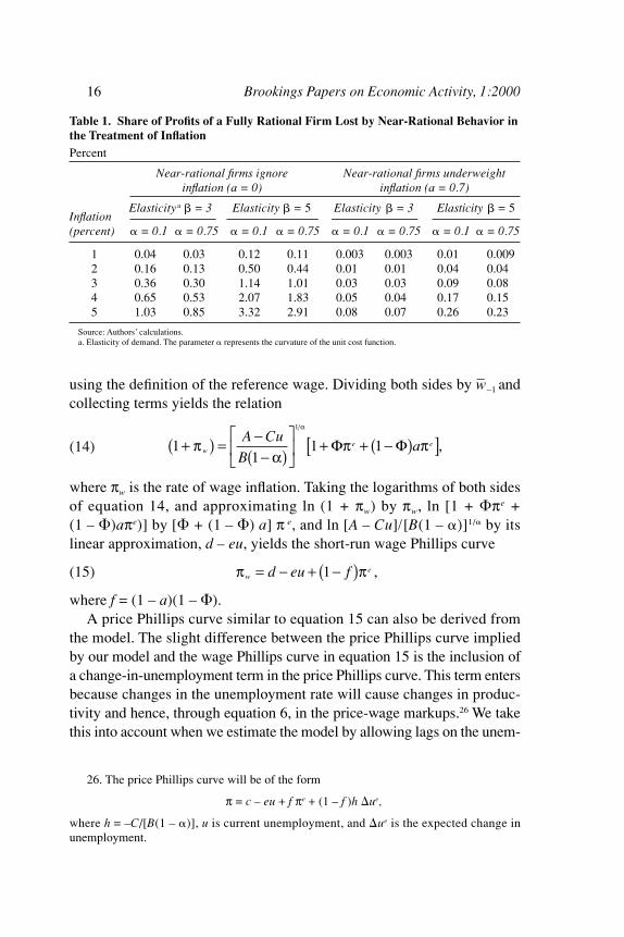
Finally, equation 9 also yields benchmark estimates of the losses dueto near-rational behavior. Table 1 shows the fraction of the profits of thefully rational firm sacrificed by the near-rational firm at different rates ofinflation for two different values of a and two different values of both �and �.

To put the values in table 1 in perspective, consider the findings ofJonathan Leonard and of Steven Davis, John Haltiwanger, and Scott Schuhthat the typical firm annually experiences shocks to demand that cause it to adjust its size up or down by roughly 10 percent.25 Failing to adjust capac-ity to accommodate such a shock would cost a firm 10 percent of its profits.Thus it does not seem hard to believe that, for the typical firm, the issue ofhow to treat inflation in setting prices is far down the list of items demand-ing managerial attention, at least as long as inflation is under 5 percent.

Implications for the Long-Run and the Short-Run Phillips Curve

The model also allows easy derivation of both a short-run Phillips curvewith given expectations of price inflation, and a long-run Phillips curvewhere actual and expected inflation must coincide. The short-run wagePhillips curve is obtained from wage-setting behavior and the equationfor the average wage. The average wage in this economy will be

(11)

Using the wage-setting behavior of the rational and near-rational firms,

(12)

which can be rewritten as

(13) – ,1

1 11

1

1

1

1

1wA Cu

Bw

A Cu

Bw ae e= −

−( )

+( ) + ( ) −

−( )

+( )− −Φ Φ

απ

απ

α α

,1

11

1 1

wA Cu

Bw

A Cu

Bwr

RnrR= −

−( )

+ −( ) −

−( )

Φ Φ

α α

α α

– .1w w wr nr= + ( )Φ Φ


25. Leonard (1987); Davis, Haltiwanger, and Schuh (1996).


using the definition of the reference wage. Dividing both sides by w� –1 andcollecting terms yields the relation

(14)

where πw is the rate of wage inflation. Taking the logarithms of both sidesof equation 14, and approximating ln (1 + πw) by πw, ln [1 + �πe + (1 – �)aπe)] by [� + (1 – �) a] π e, and ln [A – Cu]/[B(1 – �)]1/� by itslinear approximation, d – eu, yields the short-run wage Phillips curve

(15)

where f = (1 – a)(1 – �).A price Phillips curve similar to equation 15 can also be derived from

the model. The slight difference between the price Phillips curve impliedby our model and the wage Phillips curve in equation 15 is the inclusion ofa change-in-unemployment term in the price Phillips curve. This term entersbecause changes in the unemployment rate will cause changes in produc-tivity and hence, through equation 6, in the price-wage markups.26 We takethis into account when we estimate the model by allowing lags on the unem-

,1π πwed eu f= − + −( )

,11

1 1

1

+( ) = −−( )

+ + −( )[ ]π

απ π

α

we e

A Cu

BaΦ Φ


26. The price Phillips curve will be of the form

π = c – eu + f πe + (1 – f )h �ue,

where h = –C/[B(1 – �)], u is current unemployment, and �ue is the expected change inunemployment.

Table 1. Share of Profits of a Fully Rational Firm Lost by Near-Rational Behavior inthe Treatment of InflationPercent

Near-rational firms ignore Near-rational firms underweightinflation (a = 0) inflation (a = 0.7)

InflationElasticity a � = 3 Elasticity � = 5 Elasticity � = 3 Elasticity � = 5

(percent) � = 0.1 � = 0.75 � = 0.1 � = 0.75 � = 0.1 � = 0.75 � = 0.1 � = 0.75

1 0.04 0.03 0.12 0.11 0.003 0.003 0.01 0.0092 0.16 0.13 0.50 0.44 0.01 0.01 0.04 0.043 0.36 0.30 1.14 1.01 0.03 0.03 0.09 0.084 0.65 0.53 2.07 1.83 0.05 0.04 0.17 0.155 1.03 0.85 3.32 2.91 0.08 0.07 0.26 0.23

Source: Authors’ calculations.a. Elasticity of demand. The parameter � represents the curvature of the unit cost function.


ployment rate. The steady-state Phillips curves with constant unemploymentwill be unaffected by varying markups caused by varying unemployment.

The short-run Phillips curve in equation 15 should come as no sur-prise. If all inflation had been included in the mental frames of the firms,which are the wage and price setters in this model, the coefficient f wouldbe equal to zero. The near-rational firms, which constitute a fraction (1 – �) of all firms, ignore a fraction (1 – a) of inflation. As a consequence,the Phillips curve in equation 15 mimics the usual inflation-augmentedPhillips curve, but with a fraction (1 – a)(1 – �) of the expected inflationignored. Thus the Phillips curve in equation 15 is not just an artifact ofour illustrative model of price and wage setting. As long as a fraction ofinflation is ignored or underweighted in near-rational wage and pricesetting, that fraction of inflation should fail to enter the inflation augmen-tation term. A whole spectrum of other models in which various combi-nations of firms and workers ignore or underweight inflation in theirmental frames will yield similar results.

Using equation 15, the long-run Phillips curve, where actual andexpected inflation are equal, will be

(16)

where un is the natural rate of unemployment if all firms are rational. Itsvalue in this model is d/e.

The long-run Phillips curve in equation 16 will be bowed inward andthen forward bending. At zero inflation, π is zero, and therefore unem-ployment is at the natural rate. At very high inflation all firms will havegiven up being near rational. The losses from near-rational behavior willbe sufficiently large that, by equation 10, � will be close to one—so thatf, which is (1 – �)(1 – a), will be close to zero. Thus, at both very high andvery low inflation, unemployment will be close to the natural rate, whichis the level of unemployment that would occur if all firms were totallyrational. At inflation above zero, unemployment will always be below thenatural rate, since f will always be positive; however, at high rates of infla-tion the natural rate is an asymptote.

Figure 1 portrays the rate of unemployment that corresponds to differ-ent levels of inflation in the long run with benchmark parameters. We haveassumed that near-rational firms completely ignore inflation (a = 0). Wechose the parameters describing the distribution of � so that at least half of

.1

u ue

fn − = π



all firms are always fully rational (thus �ε is zero), and 95 percent of allfirms are rational by the time inflation is at 5 percent a year. We also chose� at 0.75 and an elasticity of demand (�) of 3 (which implies a value for�ε of 0.005, or 0.15 percent of normal profits), although, as we will discussbelow, these assumptions hardly matter for the shape of figure 1.

The level of inflation that maximizes the product of f and π accordingto equation 16 will minimize unemployment. For the parameter values cho-sen to create figure 1, that inflation rate is 2.6 percent. At that rate of infla-tion the long-run equilibrium rate of unemployment is 1.7 percentage pointslower than at either a rate of inflation of zero or a rate above 6 percent.27


27. Interestingly, our choices of the values of the elasticity of demand (�) and the cur-vature of the productivity function (�) hardly matter for the shape of the curve in figure 1or for the lowest sustainable rate of unemployment and its accompanying rate of inflation.Once we set the fraction of firms that are near rational at two points, we have described thecurve for a given value of a. This result reflects a finding that will surface again later whenwe estimate the model, which is discussed in more detail in the next section. That is thatthe loss function is very nearly approximated by a constant times the square of inflation, sothat the argument of the cumulative normal in our model can be very well approximatedwith two parameters.

8

6

4

2

4 5 6

Inflation (percent per year)

Unemployment (percent)

Source: Authors' calculations from calibration of the theoretical model.

Figure 1. A Hypothetical Long-Run Phillips Curve


Why does employment rise with inflation at low rates of inflation? Inour model, inflation is not underestimated, but instead it is underweightedin the reference wage used for wage setting. This has the same con-sequences as underestimation. Near-rational firms either ignore or fail to fully project inflation, so they set lower wages, and therefore also setlower prices, relative to nominal demand, than they would if they werefully rational. Since the wages of fully rational firms are affected by thewages paid by near-rational firms, both types of firms pay lower wagesthan they would if all firms were fully rational. At these lower wages,employment will be higher. These higher levels would also occur in theslightly different version of the model in which workers underestimatethe impact of inflation.28

Empirical Evidence for Near-Rational Wage and Price Setting

In this section we discuss three related types of evidence for the impor-tance of the type of behavior we describe. We begin by recounting the find-ings of Brainard and Perry’s recent analysis of a Phillips curve modelwith time-varying parameters. We then do a simple exercise estimatingPhillips curves on a split sample to see how the estimated coefficient ofinflation differs between periods of high and low inflation. Finally, we esti-mate the model described in the previous section and present estimates ofthe unemployment-minimizing rate of inflation and the employment gainsfrom being there rather than at the natural rate.

Time-Varying Parameters

In the Brainard and Perry paper that we described at the outset,29 theauthors were addressing how uncertainty affects policymaking. Theirempirical work demonstrating one key source of uncertainty revealsprecisely the departures from conventional NAIRU models that our modelpredicts. Previous work examining how the NAIRU varied over timeassumed the NAIRU framework and allowed time variation only in the


28. We have resisted the temptation to call the unemployment-minimizing rate ofinflation the optimal rate. In this model productivity also varies with the rate of inflation.Therefore, at the minimum unemployment rate, output is not at its maximum.

29. Brainard and Perry (2000).


intercept of the equation.30 Brainard and Perry applied a general Kalman fil-ter estimation that permits all the key Phillips curve parameters to vary—lagged inflation and unemployment as well as the intercept—and lets thedata choose the allocation of time variation among them. Figure 2 summa-rizes their results with CPI inflation as the dependent variable. The figureshows substantial time variation in the coefficient of the lagged inflationterm, and virtual stability in the intercept and the coefficient of the inverseunemployment rate, which they measure by the unemployment rate of 25-to 54-year-old men to account for demographic changes over time. Thecoefficient on lagged inflation is low during periods of low inflation andapproaches one only in the inflationary middle years of the sample period.

The virtual stability over time in the unemployment coefficient and theintercept in the Brainard-Perry time-varying estimates is also worthnoting. Rather than attributing the episodes of sustained low unemploy-


30. For typical applications see Stock and Watson (1998) and Gordon (1998).

3210

–1–2–3

1964 1972 1980 1988 1996

Time-varying

Recursive

Coefficient valueIntercept

0.80.70.60.50.40.30.20.1

1964 1972 1980 1988 1996

Time-varying

Recursive

Coefficient valueLagged inflation

8

7

6

5

4

1964 1972 1980 1988 1996

Time-varying

Recursive

Coefficient valueInverse unemployment

0.5

0.0

–0.5

–1.0

1964 1972 1980 1988 1996

Time-varying

Recursive

Coefficient valueProductivity

Source: Brainard and Perry (2000).

Figure 2. Recursive Least-Squares Estimates and Time-Varying Kalman Filter Estimates of Price Phillips Curve Parameters, 1960–98


ment to declines in a NAIRU that is invariant to inflation, these resultssuggest a change in price- and wage-setting behavior that accompaniedperiods of low inflation. The model described above predicts coefficientson lagged inflation that change with the inflation regime while coefficientselsewhere are constant.

Brainard and Perry compare their Kalman filter estimates with recursiveleast-squares estimates, which are also shown in figure 2. These compar-isons suggest why conventional estimation has seemed to support theNAIRU model since Franco Modigliani and Lucas Papademos introducedit in the inflationary mid-1970s.31 Before that time, lagged inflation inPhillips curves had been consistently estimated to have a coefficient wellbelow one. But the large increase in inflation in the mid-1970s corre-sponded to a period of large variance in inflation, and fixed-coefficient esti-mation has been dominated by that episode ever since. If the coefficients infact have varied over time, any procedure that assumes that they are fixedwill yield misleading results. This includes the recursive estimates, whichtreat them as fixed in each interval over which they are estimated.

Periods of Low and High Inflation

The postwar U.S. economy has experienced extended episodes of bothlow and moderately high inflation that permit direct comparison of theNAIRU model with our own. Conventional NAIRU models use a modifiedPhillips curve in which lagged inflation is taken as a measure of adaptiveinflationary expectations, and the coefficients on lagged inflation sum toone. By contrast, our model allows the possibility that the coefficient onexpected inflation will be lower in extended periods of low inflation thanin extended periods of high inflation. Absent estimation biases, we wouldexpect the coefficient to approach one in a sufficiently inflationary envi-ronment. We first look at the empirical evidence using the conventionaladaptive expectations framework. We then provide evidence using directmeasures of inflationary expectations that address Sargent’s criticism ofthe assumption that the coefficient on lagged inflation must equal one in anaccelerationist model.32 Sargent argued that a coefficient of less than oneon lagged inflation may reflect not incomplete projection of inflation, butrather forecasters’ views that the process generating inflation does not have


31. Modigliani and Papademos (1975).32. Sargent (1971).


a unit root. By using direct measures of inflationary expectations, we canrule out the possibility that our results reflect differences in how peopleform expectations rather than in how they use them.33

In order to separately estimate wage and price Phillips curves forperiods of low and high inflation, we sorted the quarters since the KoreanWar according to the average CPI inflation rate in the five-year periodending each quarter. We first classified quarters with average annualizedinflation rates below 3 percent as low-inflation quarters, and those withaverage inflation rates above 4 percent as high-inflation quarters.34 Bythis sorting, the low-inflation quarters run from 1954:1 through 1969:1 andfrom 1995:3 through 1999:4, the end of our sample period. The high-inflation quarters run from 1970:2 through 1986:1 and from 1990:4through 1993:2. As it happens, there are seventy-seven quarters both in thehigh-inflation sample and in the low-inflation sample. The mean CPI infla-tion rates in the two samples are 6.3 percent and 2.0 percent, respectively.This separation was used in half of the wage and price inflation regres-sions. In the other half we limited the low-inflation sample to quarters withinflation rates below 2.5 percent, which brought the sample size down tosixty-two quarters and reduced the mean CPI inflation rate in the low-inflation sample to 1.9 percent.

Estimates with Adaptive Expectations

The quarterly Phillips curve equations we estimated were intended tospan the specifications that analysts have used in conventional estimationof NAIRU models, except for the fact that we did not constrain the coeffi-cients on lagged inflation. To this end, we tried a large number of datacombinations and specifications on both wage and price Phillips curves,and ran each separately for the low- and high-inflation samples justdescribed. In all cases the dependent variable was an annualized inflationrate in either wages or prices, and the explanatory variables were currentor lagged values of unemployment, price inflation, and, for the wage equa-tions, trend productivity growth. For price inflation we used the CPI, theGDP deflator, and the personal consumption expenditure (PCE) deflator


33. We are grateful to a seminar participant at the Bank of Canada for suggesting thisapproach.

34. By sorting our sample on the basis of long lags of the endogenous variable, we con-siderably reduce concern about sample selection on the basis of an endogenous variable.


and estimated price Phillips curves with each. Twelve values of laggedinflation were used as explanatory variables. For wage inflation we usedthe best series available for any time period, linking private wages andsalaries as measured by the employment cost index (ECI) for 1980–99 tothe adjusted hourly earnings index for the nonfarm economy for 1961–80and to adjusted hourly earnings in manufacturing for 1954–61. Twelvelagged values of CPI inflation were used as explanatory variables. Forunemployment we used the rate for all workers (the total rate), the ratefor 25- to 54-year-old males, and Robert Shimer’s demographicallyadjusted series.35 We used the current and three lagged values of unem-ployment and, alternatively, the current and eleven lagged values. For thewage Phillips curves we used two estimates of trend productivity growth,one being a series based on work by Robert Gordon and the other theseries we constructed for our 1996 paper.36 We ran regressions with theproductivity coefficient either freely estimated or constrained to be one(for the wage inflation equations), and with just the current trend or withthe current plus seven lagged values of the trend.37

The key results are summarized in figure 3 for equations explainingwages and in figure 4 for equations explaining prices. The figures presentthe results of 144 and 72 specifications, respectively. Each point repre-sents the sum of the coefficients on lagged inflation estimated for the low-and the high-inflation samples for one specification. If the sums of the coef-ficients were similar for the two samples, the points would cluster along the 45-degree line. If they were similar and near one, the points would clusternear the upper right corner. In fact, for both wages and prices, and over thewide range of specifications and data we used, the points cluster near oneon the high-inflation axis, but on the low-inflation axis they range fromaround zero to around 0.5 for the wage equations. This is consistent withthe predictions of our model. The range on the price equations is broaderand less conclusive. The third of the observations at the highest end of therange are from equations using the PCE deflator. The mean values of thecoefficients on the high- and low-inflation axes, respectively, are 0.25 and0.82 for the wage equations and 0.60 and 0.95 for the price equations.


35. Shimer (1998).36. Gordon (1998); Akerlof, Dickens, and Perry (1996).37. All the equations also used the customary dummy variables for the guidepost period

of the 1960s and the price controls period of the 1970s, and used the difference betweeninflation with and without oil prices in 1979–80 as an additional variable.


Direct Measures of Inflationary Expectations

As in Brainard and Perry’s paper, the results just described cast doubt onconventional estimates with the NAIRU model. However, both analyses treatexpectations as adaptive and so cannot refute Sargent’s criticism that ratio-nal expectations are formed differently and that the coefficient on properlymeasured expectations might be one. We now address this issue by usingdirect measures of expected inflation as explanatory variables in place of dis-tributed lags of actual inflation rates, while maintaining our division of thesample into periods of high and low inflation. The other explanatory vari-ables are the same as those used in the regressions behind figures 3 and 4.We used the two direct measures of expected rates of inflation that are avail-able over our sample period: that from the University of Michigan’s Surveyof Consumers and that from the Federal Reserve’s Livingston Surveys.


1.25

1.00

0.75

0.50

0.25

–0.25 0 0.25 0.50 0.75 1.00 1.25

Means:Low-inflation samples 0.04High-inflation samples 0.82

Low-inflation samples

Figure 3. Wage Equations: Sum of Coefficients on Lagged Inflation in Low- and High-Inflation Samples, 1954–99

Source: Coefficient estimates from 144 regression specifications as described in the text.

High-inflation samples


Figures 5 and 6 plot the estimated coefficients on expected inflation for thevariously specified wage and price regressions, respectively. As with theresults using adaptive expectations, the coefficients on expected inflation aresubstantially different in the low- and high-inflation periods. For 288 wageequations the low- and high-period means are 0.29 and 0.85, respectively.For 144 price equations the means are 0.25 and 1.00, respectively.

These results support our general hypothesis even more convincinglythan do the results with adaptive expectations. Not only do they addressthe point that the relevant coefficient for natural rate theory is not neces-sarily the coefficient estimated with adaptive expectations, but the resultsare as clear about price inflation as they are about wage inflation.

One possible objection to the results presented here and in the next sec-tion is that the lower coefficients on inflationary expectations during peri-


1.25

1.00

0.75

0.50

0.25

–0.25 0 0.25 0.50 0.75 1.00 1.25

Means:Total CPI GDP deflator PCE deflator

Low 0.60 0.63 0.40 0.76High 0.94 0.92 0.97 0.94


Figure 4. Price Equations: Sum of Coefficients on Lagged Inflation in Low- and High-Inflation Samples, 1954–99




ods of low inflation are an artifact of measurement error. For example, if thevariance of measurement error is constant whereas the variance of trueinflationary expectations is higher in times of high inflation, then thecoefficient on expectations could be biased toward zero more in times of low inflation than in times of high inflation. We investigated this possibility. Although it is true that the variance of expectations is higher in periods of high inflation, it is also true that the sampling error in both the Survey of Consumers and the Livingston Survey is higher.In fact, the sampling error is so much higher that the computed bias ishigher in the low-inflation periods, imparting a bias against our finding thatthe coefficient on expectations is lower in periods of low inflation.

Sampling error may not be the only source of error in the survey expec-tations. Neither survey may be asking the right people with the rightweights. In an attempt to approximate how much error this problem might


1.25

1.00

0.75

0.50

0.25

–0.25 0 0.25 0.50 0.75 1.00 1.25

Means:Low-inflation samples 0.29High-inflation samples 0.85


Figure 5. Wage Equations: Coefficients on Price Expectations Variables in Low- and High-Inflation Samples, 1954–99




introduce, we computed the bias that would be caused if the measure-ment error variance in expectations were equal to the variance of the resid-ual of a regression of one of our survey expectations on the other. Againwe found that the measurement error variance grew faster than the condi-tional variance of the expectations, so that the bias caused thereby wouldwork against our finding that the coefficient on expectations was lowerwhen inflation was low.

Estimating the Model

Previously we showed how a Phillips curve–type relation can bederived from our theoretical model (equation 15). In this section wepresent estimates of the model and of the rate of inflation that permits the


1.25

1.00

0.75

0.50

0.25

–0.25 0 0.25 0.50 0.75 1.00 1.25

Means:Total CPI GDP deflator PCE deflator

Low 0.25 0.56 0.00 0.20High 1.00 1.16 0.94 0.91


Figure 6. Price Equations: Coefficients on Price Expectations Variables in Low- and High-Inflation Samples, 1954–99




lowest sustainable level of unemployment. We also show the gain inemployment compared with operating at the natural rate. This sectionwill first discuss the specification of the model we estimate, then ourbenchmark results, and finally, an analysis of their robustness.

Specifications

In theory, with a large enough sample, it would be possible to estimatethe full model presented above. The elasticity of demand (�), the parame-ter for the curvature of the unit cost function (�), and the parameters of thedistribution of rationality thresholds (� and �) all have different effectson the objective function. However, in practice it was impossible to esti-mate more than the mean of the distribution of rationality thresholds andone of the other parameters. The reason is that all three of them—the elas-ticity of demand, the curvature of the productivity function, and the stan-dard deviation of the distribution of rationality thresholds—act in muchthe same way to determine the impact of past rates of inflation on thecumulative normal term (see equation 15).

This lack of identification in practice can be understood if we considera Taylor series approximation to the argument of the cumulative normal inequation 15, expanded around a value of zero inflation. There is no reasonto expect that the argument will be exactly zero at zero inflation, so the con-stant term will likely be present. As noted, the first derivative of the firm’sloss function with respect to inflation is zero at zero inflation and very smallat most rates of inflation less than 10 percent. Thus the first-order term ofthe Taylor series expansion of the argument of the cumulative normal willalso be zero. Second- and higher-order terms will be present, but our analy-sis of the loss function suggests that, with inflation between zero and 10percent, and with reasonable values for the elasticity of demand, thecurvature of the unit cost function, and the standard deviation of the distri-bution of rationality thresholds, the third-order and higher terms are unim-portant. An approximation of the loss function of the form Eπ2, where theconstant E was chosen so that the approximation was exactly equal to theloss at 5 percent inflation, was never off by more than 3 percent of the loss.One parameter is all that is necessary to capture the effects of all three para-meters from the model (�, �, and �) on the derivative of the argument of thecumulative normal with respect to inflation.

We thus estimate a Phillips curve of the form



(17)

where π is the rate of inflation, � is the cumulative standard normal den-sity function, πe is inflationary expectations, u is a term capturing theeffects of current and lagged unemployment on inflation, X is a vector ofdummy variables for oil shocks and price controls, is the error term,and d, D, E, e, and g are parameters to be estimated.38

The term πL represents the effects of past inflation on the likelihood thatpeople will act rationally toward inflation. Our theory tells us nothing aboutthe way in which inflation should matter other than the sign of E, so we proxyπL with several different, parsimonious specifications. The first is a geomet-rically declining, weighted moving average of past values of inflation:

(18)

where is a parameter to be estimated. Alternatively we estimate πL as

(19)

where the parameter � is estimated. Our final two specifications for πL treatit as a four-year moving average of past inflation with equal weights, orwith the relative weights of quarters from each year estimated (three addi-tional parameters).

It is standard practice in Phillips curve estimation to proxy inflationaryexpectations with lagged values of inflation. In many specifications dis-cussed below we follow that tradition. When we do, we use either atwelve-quarter unrestricted lag or one of the methods used to construct πL

to construct πe. However, we also want to rule out the possibility that

,

1

1

11

24

11

24π

λ π

λλ

λ

L

iii

ii

i

i=

−( )

−( )

−=

<

=<

∑

∑

– ,1 1 1π δ π δπL L L= ( ) +− −

.2π π πt Lt te

t t td D E eu gX= + +( ) − + +Φ


38. This specification ignores the parameter a from the theoretical model. In theory thatparameter could be estimated, but we do not take the theoretical model that literally. Insteadwe imagine that there is a continuum of reactions to increasing inflation, with people puttingmore and more weight on it until their behavior resembles that of the rational economicactor in the standard model. The model we estimate here can be thought of as a model wherea fraction (1 – �) of people are ignoring inflation. Or the � function can be thought of asapproximating a more general function that reflects how much weight the average personis putting on inflation in making economic decisions.


changes in the coefficient on πe might reflect changes in the process bywhich expectations are formed rather than how they are used. Thus we alsouse direct survey measures of inflationary expectations for πe in somespecifications.

Our different specifications include several different measures of unem-ployment and different numbers of lags. The unemployment term, u, isconstructed using one of three data series. The first is the aggregate U.S.unemployment rate from the Current Population Survey of the Bureau ofLabor Statistics. Because this variable may be influenced by changingdemographics, we have also considered two alternative measures: theunemployment rate for prime-age males and Shimer’s demographicallycorrected series.39 We also vary the number of unemployment lags fromzero to eleven quarters.

For the dependent variable we variously use four different measures ofinflation: the annualized percentage change in the urban consumer priceindex, the GDP deflator, the PCE deflator, and the index of wage and salarycompensation constructed by Brainard and Perry.40 When we use the per-centage change in the compensation index as the dependent variable, wesubtract off a measure of trend productivity growth. The three specifica-tions of this trend are a measure based on Gordon, the measure we con-structed for our 1996 paper, and a sixteen-quarter moving average.41

The form of the Phillips curve here is similar in some respects to theone in our 1996 paper that modeled the implications of downward nominalwage rigidity. Therefore we also examine whether we can successfullyestimate a Phillips curve that embodies the insights from that model aswell as the current one. Below we estimate a number of specificationsthat augment equation 17 with the term for nominal rigidity from thatprevious paper.42 When we nest that model, we must also estimate its keyparameter—the standard deviation of desired wage changes—along withthe other parameters from the current model.43


39. Shimer (1998).40. Brainard and Perry (2000).41. Gordon (1998); Akerlof, Dickens, and Perry (1996).42. The inclusion of the term for nominal rigidity could be motivated if we included firm

profitability or firm-specific labor market considerations in the productivity function. Thatwould produce heterogeneity in desired wage setting, with firms constrained by the floor of nonominal wage decrease forced to pay a higher wage as in the model in our previous paper.

43. See Akerlof, Dickens, and Perry (1996, appendix A) for its specification. We leaveout the term for the change in profits, which could not be robustly estimated.


The model was estimated with quarterly U.S. data from the first quar-ter of 1954 through the last quarter of 1999, although we vary the enddate in some specifications to check the extent to which our results dependon the experience of the 1990s. Data sources and the specification of thedummy variables for price controls and oil shocks can be found in table A1in the appendix.44 All the parameters of the model were estimated simul-taneously by nonlinear least squares.

Results

Table 2 presents results for four different estimates with five types ofvariation: in the dependent variable, in the method of constructing πe andπL, in the unemployment measure and its lags, in the sample period, andin the inclusion of the term for nominal rigidity.

Our first focus of attention is the estimated value of the cumulativenormal multiplying inflationary expectations when inflation is zero. Inthe theoretical model this corresponds to the fraction of firms behaving ina fully rational fashion at zero inflation. The model predicts that this frac-tion will be less than unity, and that as inflation increases above zero, thefraction of rational firms will rise. Both of these predictions yield tests ofthe model.

The NAIRU specification for the Phillips curve is nested in our modeland can be obtained if the value of D is sufficiently high. For example, if Dwere 2 or higher, the coefficient on inflationary expectations would neverfall below 0.97, and there would be little room for changing experiencewith inflation to affect the coefficient on inflationary expectations. All ofthe four estimated values of D imply coefficients on expected inflation of0.5 or less at zero inflation. The lowest implies a coefficient of 0.19. In allfour cases a value of D that would imply a coefficient of 0.9 or greater(1.28) can be rejected at conventional levels of significance.

The instantaneous effect of increasing inflation above zero can be com-puted as one minus the cumulative normal evaluated at D, divided by thesum of the coefficients on unemployment and its lags. Those values areabout –1.2 or larger (in absolute value) in the specifications presented here.Thus, to a first-order approximation, raising inflation from zero to 1 percentwill cause a reduction in unemployment of 1.2 percentage points or more.


44. We use dummy variables rather than an import price or energy price measure becausewe believe that these were atypical events that had atypical effects on the economy.


Tab

le 2

. E

stim

ated

Par

amet

ers

for

the

Nea

r-R

atio

nal P

hilli

ps C

urve

a

Dep

ende

nt v

aria

ble

Com

pens

atio

nIn

depe

nden

t var

iabl

ein

dex

min

usan

d ch

arac

teri

stic

sC

PI

GD

P d

eflat

orP

CE

defl

ator

prod

ucti

vity

gro

wth

Con

stan

t0.

038

0.02

80.

024

0.01

8(0

.008

)(0

.008

)(0

.012

)(0

.003

)U

nem

ploy

men

t–0

.51

–0.4

5–0

.43

–0.4

2(0

.12)

(0.1

2)(0

.18)

(0.0

7)D

(con

stan

t in

coef

fici

ent o

n ex

pect

atio

ns)

–0.4

7–0

.88

0.02

–0.3

3(0

.36)

(0.4

5)(0

.60)

(0.2

3)E

(coe

ffici

ent o

f π L

2in

coe

ffici

ent o

n48

82,

824

1,17

21,

309

expe

ctat

ions

)(1

52)

(1,1

20)

(708

)(3

68)

Sta

ndar

d de

viat

ion

of d

esir

ed w

age

chan

geTe

rm n

ot in

clud

edTe

rm n

ot in

clud

ed0.

022

Term

not

incl

uded

from

term

for

nom

inal

rig

idit

y(0

.014

)M

etho

d fo

r co

nstr

ucti

ng π

LG

eom

etri

c16

-qua

rter

mov

ing

Geo

met

ric

Lin

ear

aver

age

(equ

al w

eigh

ts)

Met

hod

for

cons

truc

ting

πe

Sur

veys

of

cons

umer

s12

unr

estr

icte

d la

gsG

eom

etri

cL

ivin

gsto

nU

nem

ploy

men

t mea

sure

and

num

ber

Tota

l; 0

lags

Tota

l; 1

1 la

gsS

him

er; 7

lags

Mal

e; 3

lags

of la

gs

Sam

ple

peri

od19

54:1

–198

9:4

1954

:1–1

999:

419

54:1

–199

9:4

1954

:1–1

999:

4N

atur

al r

ate

of u

nem

ploy

men

t (pe

rcen

t)7.

56.

45.

64.

4In

flat

ion

at lo

wes

t sus

tain

able

unem

ploy

men

t rat

e (p

erce

nt)

3.4

1.6

2.4

2.0

Low

est s

usta

inab

le u

nem

ploy

men

t rat

e(p

erce

nt)

4.5

4.4

4.7

2.3

Dur

bin-

Wat

son

stat

isti

c1.

42.

01.

91.

1R

20.

824

0.69

80.

717

0.72

9

Sou

rce:

Aut

hors

’cal

cula

tion

s.a.

Sta

ndar

d er

rors

are

in p

aren

thes

es.


The term that most distinguishes our model from that of the textbooksis the coefficient of the square of lagged inflation in the cumulative normalmultiplying inflationary expectations (E). If E is zero, the coefficient onexpectations will not vary with past rates of inflation. Our theory says itshould, and that is what we find in each of the specifications we have esti-mated. In all four specifications presented above, E is large, and more than1.65 times its estimated standard error. Going from zero to 5 percent infla-tion would increase the argument of the cumulative normal by 1.2 to 7.0,depending on the specification. Except in specifications with CPI inflationas the dependent variable, the coefficient on inflationary expectations isabove 0.95 by the time inflation has reached 4 percent. For the CPI speci-fication the coefficient is 0.6 at 4 percent inflation and rises above 0.95 atabout 6.5 percent.

Besides allowing us to estimate the effect of inflation on the use ofinflationary expectations, estimating our model also allows us to calculatethe lowest sustainable rate of unemployment and the accompanying rateof inflation. We have computed these rates of inflation for each of the fourmodels in table 2 from the estimated parameters numerically. We havealso computed the natural rate in each model and the lowest sustainablerate of unemployment. Inflation at that unemployment rate ranges from1.6 to 3.4 percent. The difference between the natural rate and the lowestsustainable rate of unemployment ranges from 1.5 to 3.1 percentagepoints. Figure 7 shows the long-run relationship between inflation andunemployment implied by each of the four specifications estimated intable 2.

The values of the coefficient of inflationary expectations implied byour parameter estimates are plotted in figure 8 for each of our four spec-ifications. In all cases the coefficient values vary considerably over thesample. In all four specifications the coefficient on inflation reaches amaximum value of one for at least a year at some point during the sam-ple period in the early to mid-1970s. The four specifications differ in theexact timing of the increase in the 1970s, in how the 1950s and the 1990sare treated, and in the date of the end of the period of a coefficient ofone on inflation.

These figures can be compared with the time path Brainard and Perryestimated for the coefficient on inflation.45 Our estimates imply consider-


45. Brainard and Perry (2000).


10 8 6 4 2 0

12

34

56

78

9

Tot

al u

nem

ploy

men

t (pe

rcen

t)

Fig

ure

7. L

ong-

Run

Inf

lati

on-U

nem

ploy

men

t R

elat

ion

Est

imat

ed w

ith

Var

ious

Pri

ce I

ndex

es

Cha

nge

in C

PI (

perc

ent p

er y

ear)

10 8 6 4 2 0

12

34

56

78

9

Tot

al u

nem

ploy

men

t (pe

rcen

t)

Cha

nge

in G

DP

defl

ator

(pe

rcen

t per

yea

r)

10 8 6 4 2 0

12

34

56

78

9

Shim

er u

nem

ploy

men

ta (

perc

ent)

Cha

nge

in P

CE

def

lato

r (p

erce

nt p

er y

ear)

10 8 6 4 2 0

12

34

56

78

9

Prim

e-ag

e m

ale

unem

ploy

men

t (pe

rcen

t)

Cha

nge

in E

CI

min

us p

rodu

ctiv

ity tr

end

(per

cent

per

yea

r)

Sour

ce: A

utho

rs’

calc

ulat

ions

fro

m th

e es

timat

ed p

aram

eter

s re

port

ed in

tabl

e 2.

a. S

him

er’s

(19

98)

dem

ogra

phic

ally

adj

uste

d un

empl

oym

ent r

ate.


1.0

0.8

0.6

0.4

0.2

1955

1960

1965

1970

1975

1980

1985

1990

1995

Fig

ure

8. C

oeff

icie

nt o

n In

flat

ion

in M

odel

s w

ith

Var

ious

Pri

ce I

ndex

es, 1

954–

99

Coe

ffic

ient

val

ue

Sour

ce: A

utho

rs' c

alcu

latio

ns f

rom

the

estim

ated

par

amet

ers

repo

rted

in ta

ble

2.

CP

I

1.0

0.8

0.6

0.4

0.2

1955

1960

1965

1970

1975

1980

1985

1990

1995

Coe

ffic

ient

val

ueG

DP

def

lato

r

1.0

0.8

0.6

0.4

0.2

1955

1960

1965

1970

1975

1980

1985

1990

1995

Coe

ffic

ient

val

ueP

CE

def

lato

r

1.0

0.8

0.6

0.4

0.2

1955

1960

1965

1970

1975

1980

1985

1990

1995

Coe

ffic

ient

val

ueE

CI

min

us p

rodu

ctiv

ity

tren

d


ably more abrupt changes and more persistence. They also imply morevariation. However, it must be remembered that the method Brainard andPerry used to estimate their values for the coefficient on inflation imposessmoothness on the changes. When we smooth our estimates (results notshown), they begin to resemble the time path that Brainard and Perryfound, with one major difference. The Brainard-Perry estimates peakearlier and fall off more abruptly than our smoothed estimates.

We have varied the specifications presented above to anticipate possibleobjections to our results. The specification with the CPI as the dependentvariable, which is estimated using only data through 1989:4, shows thatour results do not depend on the experience of the 1990s, which may beatypical. Since nonlinear estimation is difficult when many parametersare being estimated, we have generally used very parsimonious specifica-tions for the lags on past price inflation when constructing inflationaryexpectations. One might object that this parsimony forces the coefficienton inflation to do the work that a richer lag structure would do. The spec-ification where the GDP deflator is the dependent variable answers thisby matching the richest possible lag structure for price expectations(twelve-quarter unrestricted) with the most parsimonious specification ofthe term in the coefficient of expectations (a sixteen-quarter equallyweighted moving average with no free parameters). Likewise, in mostspecifications, the inclusion of lagged unemployment, or our term fornominal rigidity, or both does not change our fundamental results.

Our Durbin-Watson statistics for the two specifications using surveyexpectations show considerable serial correlation. We have not attemptedto correct for this problem because we lack a credible instrument for priceexpectations, which are endogenous with respect to the error in the Phillipscurve. We are unhappy with this drawback of the analysis, but estimates ofour model that we have tried using simulated data suggest that the bias fromignoring the serial correlation in the parameters we care about is minor.

Robustness of the Results

As noted above, there are many aspects of the specification that are notdictated by the theory. Our approach to this problem has been to estimatea wide array of different specifications to determine whether our primaryresults are sensitive to changes in the specification.

Because both the estimation of the model and the numerical analysisof the results currently require human intervention, we have not been able



to mechanize the process of sensitivity testing. Thus we have not been ableto do an exhaustive specification search. Instead we estimated 218 differ-ent specifications, many of which were run to test specific concerns.However, most were chosen randomly.46 Our survey of the results of thesespecifications yields the following generalizations.

The most important is that nearly all the point estimates imply that sig-nificant gains in employment are possible by increasing inflation from zeroto a rate above 1.5 percent. This can be seen in figure 9, which plots foreach specification the rate of inflation at the lowest sustainable unem-ployment rate and the reduction in unemployment that one obtains fromincreasing inflation from zero to that rate. In only twelve specificationswas the estimated gain less than 1 percentage point, and in only one wasit negligible. This specification was a wage Phillips curve with a rich lagstructure for price expectations in which the inflation term in the coeffi-cient on expectations was constrained to be an equally weighted, sixteen-quarter moving average of past inflation. Allowing a richer specificationfor the impact of inflation on the use of expectations eliminates this result.Of the other eleven specifications where the estimated impact is less than1 percent, all are at least a half a percentage point. Most of the specifica-tions are wage equations, and none use the PCE deflator as the dependentvariable. Only one uses survey expectations. In no case are the parame-ters of the inflation coefficient very precisely estimated, so that valuesmore typical of other specifications cannot be ruled out.

A second generalization is that it is not possible to robustly distinguishthe relative importance of the effects of nominal rigidity and those of nearrationality. The majority of specifications that included our term for theeffects of nominal rigidity give results like those for the PCE in table 2.These do suggest a role for both nominal rigidity and near rationality.However, in many specifications that include both effects, the effect of pastinflation on the coefficient of expectations is not measured precisely, beingabout the same size as its estimated standard error.47 In other cases, the


46. We set a goal of 200 specifications, met that goal, and then estimated a few more tocheck specific concerns that arose in the process of evaluating the original 200 specifica-tions. In randomly choosing specifications we allowed all options with equal probability,except that we found that the twelve-quarter unrestricted lag on inflation for the price expec-tations term was always computationally burdensome, so we did not include those specifi-cations in those that were randomly chosen.

47. In contrast, when the term for nominal rigidity was not included, the coefficient onthe square of past inflation was nearly always at least 1.7 times its estimated standard erroror more.


optimization routine was trying to drive estimates of the standard deviationof desired wage changes to zero. In six specifications not represented infigure 9, we obtained converged estimates for the parameters, but theestimated values for � were sufficiently large that there was no single rateof inflation at which the unemployment rate was minimized. It simplyfell to the natural rate asymptotically as in the models estimated for our1996 paper.48

We encountered few problems with applying nonlinear estimation. Wedid look for and find a few cases where there were multiple local mini-mums, but these reflected minor differences in the lag structures that werenot substantive. Of the 218 specifications we estimated, we were unable toobtain converged values for about 30. This might be a serious concernbecause, under the hypothesis of fully rational behavior, the model’sparameters are not identified. It might be that the nonlinear estimation pro-gram is trying to drive the constant term in the coefficient on inflationaryexpectations to infinity in order to drive the coefficient on expectations to


48. Akerlof, Dickens, and Perry (1996).

8

6

4

2

2 4 6 8

Rate of inflation at the lowest sustainable unemployment rate (percent per year)

Unemployment rate at zero inflation minus the minimum unemployment rate (percentage points)

Total or Shimer unemploymentPrime-age male unemployment

Figure 9. Robustness Analysis for the Nonlinear Model



one.49 However, this is not what was happening in any of the cases ofconvergence problems that we encountered.50

Overall, the results from estimating our model support the theory we have laid out. They suggest that macroeconomic policy should aim for a rate of inflation in the range of 1.5 to 4 percent. Either higher orlower rates seem likely to result in lower output and employment.

Conclusion

This paper offers an alternative to natural rate models of unemploy-ment. Natural rate models provide a wonderful economics “just-so” story,based on the idea that firms and workers take full account of expectedinflation in setting current wages and prices. This behavior produces aunique long-run unemployment rate, the natural rate, that is consistentwith any steady rate of inflation, and a short-run Phillips curve in whichunemployment above or below the natural rate causes inflation to decel-erate or accelerate.

Our model of the macroeconomy rests on different behavioral under-pinnings, which are supported by a range of related evidence, includingthe psychological literature on decisionmaking and perception, direct sur-vey evidence on how people react to inflation, and the advice of compen-sation professionals. We propose that when inflation is low it is notespecially salient, and wage and price setting will respond less than pro-portionally to expected inflation. At sufficiently high rates of inflation, bycontrast, anticipating inflation becomes important, and wage and pricesetting responds fully to expected inflation. This behavioral differencebetween our model and the natural rate model has significant implicationsboth for estimating the relation between inflation and real activity in themacroeconomy and for informing the conduct of macroeconomic policy.


49. When we generated simulated data with a standard Phillips curve model andattempted to estimate our model on it, this is what happened.

50. Instead we had one of three other problems. Either the program was trying to drive� to zero. Or the program was driving the constant term in the coefficient of expectationsto negative infinity, and the coefficient on the square of past inflation to infinity, to eliminatecoefficient values between one and the lower floor. Or, in some very rich specifications, thefirst derivatives of a group of unrelated parameters became so close to collinear that it wasimpossible to invert the approximation to the Hessian used in the maximization routine.


Our model is supported by the evidence. In a conventional Phillipscurve, estimates of coefficients on expected inflation, whether measured bylagged inflation or by direct surveys of expectations, are greater wheninflation is high than when it is low. Estimates of our model provide furthersupport. Rather than a natural rate of unemployment that is invariant to therate of inflation, our model traces out a range of equilibrium unemploy-ment rates associated with different ongoing inflation rates. The lowestsustainable unemployment rate is the minimum of this range. The naturalunemployment rate is a special case: it is the equilibrium unemploymentrate at high inflation rates (and, ignoring downward wage rigidity, at zeroinflation). The natural rate is noticeably higher than the lowest sustain-able unemployment rate. The rate of inflation that accompanies the low-est sustainable unemployment rate is low, perhaps not far from currentvalues, but not zero. Operating with inflation either higher or lower leadsto a higher rate of unemployment in the long run.

The distinctive feature of our model is especially important for estima-tion. In recent years, as low inflation rates have come to be the norm,NAIRUs estimated from the empirical counterpart of the natural ratemodel have proved to be misleading guides to policymakers and economicanalysts. In the mid-1990s these models typically projected 6 percent asthe lowest sustainable unemployment rate, yet real output has grown at a4 percent annual rate since then, and the unemployment rate has fallen aslow as 3.9 percent. The NAIRUs estimated for the early 1960s, the previ-ous period of moderate inflation, also appear unrealistic. When adapted forestimation, the model we have developed should provide more useful esti-mates of the attainable levels of employment to serve as a guide for stabi-lization policy and as an anchor to longer-run projections.

Not only does our model fit the data better than NAIRU models, it isalso more cogent theoretically. NAIRU models serve well as what IrvingFisher might call “the first approximation.” They are derived from theassumption that all people behave according to what economists call eco-nomic rationality, or else their deviations from that behavior are totallyrandom. This paper relies, as a first approximation, on exactly such eco-nomic thinking. But Fisher also made “a Second [and even a Third]Approximation.”51 With aggregate Phillips curves, such further approxi-mations involve departures from perfectly rational decisionmaking. The


51. Fisher (1930).


evidence available on the subject suggests that, in setting wages and prices,the lay public do not use the same model of the economy as economists.Given the complexity of their decisions and, for the most part, their lack oftraining as economists, it would, indeed, be surprising if they did. It is thushighly unlikely that the welter of interdependent, intuitively based deci-sions of a real economy will produce a coefficient of inflationary expecta-tions on wage and price inflation that is always exactly one. This paper hasoffered a theory for such a departure as price and wage setters under-adjust for inflation when it is not very salient and when the cost of suchbehavior is low. This theory yields a lowest sustainable rate of unemploy-ment and an accompanying rate of inflation. It also fits the facts.



A P P E N D I X A

Table A1. Data Sources and Variable Construction

Data series Source and description

Consumer price index Bureau of Labor Statistics (BLS) official data on the season-(CPI) ally adjusted average of the CPI-U, 1982–84 = 100. An exper-

imental CPI calculated using geometric means, CPI-U-XG,was used for the period 1990:1 to 1998:4. The CPI-U-XG wasseasonally adjusted using quarterly dummies. Data wereextracted from the BLS website’s Selective Access page,www.bls.gov/sahome.html. We used quarterly averages of thechange in the logarithms of monthly data. (The CPI-U-XGdata were not used for some of the specifications in the robust-ness check.)

Gross domestic product Bureau of Economic Analysis (BEA) official data reflecting(GDP) deflator the October 1999 benchmark revision for data back to 1959:2.

We used unrevised data before 1959:2 by necessity. Data wereextracted from the BEA website, www.bea.doc.gov. We usedquarterly averages of the change in the logarithms of monthlydata.

Personal consumption BEA official data reflecting the October 1999 benchmark expenditure (PCE) revision for data back to 1959:2. We used unrevised data deflator before 1959:2 by necessity. Data were extracted from the BEA

website. We used quarterly averages of the change in the loga-rithms of monthly data.

Wage inflation This series comprises the best available BLS series for eachtime period: employment cost index (ECI) wages and salariesfor 1980:2 through 1999:4, the adjusted hourly earnings indexfor the nonfarm economy for 1964:2 through 1980:1, andadjusted hourly earnings in manufacturing for 1954:1 through1964:1. We use the change in the logarithm of quarterly data.

ECI wages and salaries BLS official data on seasonally adjusted, private industrywages and salaries of all workers, extracted from the BLSwebsite’s Selective Access page.

Adjusted hourly earnings BLS official data on seasonally adjusted, current dollar index average hourly earnings (1977 weights) in the nonfarm econ-

omy. Data were extracted from the BLS website’s SelectiveAccess page.

Adjusted hourly earnings BLS official data on seasonally adjusted, current dollar in manufacturing average hourly earnings (1977 weights) in the manufacturing

sector. Data were extracted from an unpublished BLS series.

(continued)



Table A1. (continued)


(continued)

Gordon productivity trend We constructed this variable using estimates of trend produc-tivity over several time periods provided by Robert Gordon,Northwestern University. We smoothed the transitions so thatthe variable is equal to 0.0263 from the start of the samplethrough 1971:2, after which it changes over nine quarters to avalue of 0.0124, which is maintained through 1986:2, afterwhich it drops to 0.0094 over eight quarters. From 1988:2through 1994:4 it is constant and then rises over seven quar-ters to 0.0153, where it remains until the end of our sample.The exact series is available from the authors by request.

Akerlof-Dickens-Perry This variable is equal to 0.0230 from the beginning of ourproductivity trend sample through 1973:4, then declines over nine quarters to a

value of 0.0100, where it remains through the rest of the sam-ple. The values for the quarters 1974:1 through 1975:4 are0.0216, 0.0201, 0.0187, 0.0172, 0.0158, 0.0144, 0.0129, and0.0115.

Surveys of Consumers The University of Michigan’s Survey Research Center, whichInflation Expectations conducts the Surveys of Consumers, asks its respondents howseries much they expect prices to go up or down on average during

the next twelve months. We use the median response to thesurvey in the last month of the previous quarter as a measureof inflationary expectations. Studies of this series suggest thatit provides the most accurate forecast of inflation one quarterahead. A complete survey description can be found athttp://athena.sca.isr.umich.edu/scripts/contents.asp.

Livingston Survey of This survey was originally conducted by Joseph Livingston, aInflation Expectations journalist with the Philadelphia Inquirer, and has been contin-

ued by the Philadelphia Federal Reserve Bank since his deathin 1990. The survey is conducted every January and June andasks respondents, who are professional economists, their fore-cast for the level of the CPI six months hence. We use theforecast of the inflation rate made in January for the secondand third quarters and the forecast made in June for the fourthand following first quarters. See http://www.phil.frb.org/files/liv/document.html for a complete description of thesurvey.

Unemployment rate BLS official data on the total unemployment rate among thenation’s labor force. Data were extracted from the BLS web-site’s Selective Access page at http://www.bls.gov/webapps/legacy/cpsatab9.htm.



Table A1. (continued)


Unemployment rate BLS official data of the unemployment rate among men agedfor males aged 25–54 25–54 in the labor force. Data were extracted from the BLS

website’s Selective Access page at http://www.bls.gov/webapps/legacy/cpsatab9.htm.

Shimer demographically Robert Shimer’s demographically adjusted unemploymentadjusted unemployment rate. For full details see Shimer (1998). Values for 1998:3rate through 1999:4 are too recent to be in his series, so we took

the arithmetic average of the difference between the Shimerseries and the total unemployment rate from 1954 to 1998 andadded that to the total unemployment rate to arrive at valuesfor the Shimer series.

Guidepost dummy A dummy variable set equal to one from 1964:1 through1966:2. This was used only in the split-sample regressions.

Wage and price controls A dummy variable set equal to one from 1971:3 throughPhase One dummy 1972:4.

Wage and price controls A dummy variable set equal to one from 1973:1 throughPhase Two and 1973 1974:1.supply shocks dummy

Wage and price controls A dummy variable set equal to one from 1974:2 throughremoval dummy 1975:1.

1979 oil price shock A dummy variable set equal to one from 1979:1 to 1980:1 anddummy for 1981:1.

Price wedge The change in the total CPI-U minus the change in the CPI-Uless food and energy. Used as an alternative to the above dum-mies in some of the split-sample regressions to account forfluctuations in food and energy prices. Data for both serieswere extracted from the BLS website’s Selective Access page.This variable was used only in the split-sample regressions.



Comments andDiscussion

Truman F. Bewley: I would like to interpret what this paper says in termsof my own experience interviewing employers about wage and employ-ment policies. The paper’s main assertion is that the perceived external rateof wage inflation has less impact on a firm’s wage policy when the rate ofinflation is low than when it is high. I will suggest that there may be anexplanation of this phenomenon different from that given by the authors.The phenomenon itself is, no doubt, real, given their persuasive empiricalresults. However, the weak feedback of inflation on wages at low rates ofwage inflation may have an explanation involving the mechanics of wagesetting and may have little to do with near-rational behavior.

In order to present my explanation, I have to describe some things Iobserved. The authors make the Keynesian assumption that moraledepends on the relationship between a firm’s wages and a reference wage,which is roughly the average of wages of other firms competing in thesame labor market. I do not think this assumption is correct. Most employ-ers that I have talked to say they think their workers have only a very vagueidea about pay rates outside their own firm. External pay rates thereforehave little impact on morale. This is especially true in nonunion com-panies. Instead workers focus almost entirely on internal comparisons:the wages they use as references are their own past pay and the pay of co-workers at the same workplace. Enough employees know each other’s pay that comparisons internal to a firm are an important compen-sation issue, at least for workers who have long-term, full-time jobs. If payrates are internally inequitable, employees complain and morale fallsapart, causing management major problems. Past pay is an obvious refer-ence, since everybody remembers his or her own compensation history.

45


The importance of this reference wage makes it difficult to cut nomi-nal pay.

Because of the significance of internal pay equity, firms normally havea strict internal pay structure that relates pay to tenure on the job, to skill,and to many other things, such as experience and job level. Internal struc-tures vary in form from firm to firm. They are part of a firm’s culture andmust be followed rigorously if a firm is to remain healthy. The structuremay be described explicitly in a booklet, especially if the firm is large. Thisdocument gives instructions to the managers who actually determine thepay of individual workers.

The relationship between the pay of different firms is the result of labormarket pressures. That is, the overall level of the pay structure is determinedby the ability to recruit and retain workers. Firms usually adjust the wholelevel of their structure, moving pay rates at different levels in concert.

It is very risky for a firm to cut the nominal pay of individual workers,unless the firm is in danger of closing and its work force clearly under-stands this danger. It may be possible, however, to reduce the nominal levelof the pay structure without cutting the pay of any worker. There is animportant distinction between the level of a pay structure and the level ofindividual workers’ pay, a matter to which I will return. It may also berisky to allow the purchasing power of workers’ pay to fall, althoughreductions in the real value of pay have less serious consequences than donominal pay cuts.

The choice of pay structure level is a strategic business decision dis-cussed at high levels of management. In making this selection, businessleaders make use of labor market surveys and look at their own experi-ence in recruiting and retaining workers. They also take account of the factthat, if they raise the level of pay today, it will remain high in the future.

I hear a lot about this last point now. I am currently surveying pricingpractices, and so I talk to businesspeople almost every day. Some say thatthey are not now increasing pay to ease labor shortages, because they knowthey will not be able to reverse the increases during the next economicdownturn.

It is important that, in setting pay levels, businesspeople look at wagesurveys. They buy surveys, make their own surveys, try to project rates ofwage inflation, and look at inflation as measured by the consumer priceindex as an indicator of what other firms will do with regard to pay. Theyalso talk to competitors in the labor market and in the product market.



They discuss what they themselves are doing with their pay structures,without giving away information that would help other firms compete withthem in product markets. Employers need this information to be sure theywill pay enough to recruit and retain labor.

Because employers discuss wage setting among themselves, there maynot be a direct and mechanical feedback from projected wage increasesto wage policy, as the paper assumes. Through mutual consultation,businesspeople can, I believe, coordinate a slowdown of wage increases.I do not mean conscious coordination and am not implying collusion, butthey may create an atmosphere that decreases the size of the pay increasesperceived as needed. Such an ambience would be beyond the control ofany one firm, but would nevertheless be achieved. It is not clear how muchcoordination occurs in this way, but businesses do keep each otherinformed as to what they are doing with pay levels.

I now turn to the distinction between the pay of individual workers andthe level of a pay structure. The former tends to increase over time,because workers rise through the internal pay structure as they acquireseniority, gain skills and experience, and become more valuable to thecompany. Workers in unskilled jobs may hit a pay ceiling after two or threeyears. But there are many skilled workers in the U.S. economy, and inmany firms these well-paid workers account for a large share of laborcosts. These workers may continue to rise in the pay structure throughouttheir career.

Because most people are rising in the pay structure, they receive payincreases every year even if the structure stays constant. If there is only alittle inflation in the cost of living, these increases might exceed that rateof inflation. A company can even decrease its pay structure while givingeverybody real and nominal increases.

A firm’s average cost of labor and its average and marginal cost of out-put are determined by the level of the pay structure. Hence, if a firm givesan average wage increase of 5 percent, it does not follow that its averagecost of labor rises by 5 percent. It may even decrease. The impact on theaverage cost of labor depends on the steepness of the company’s internalpay structure, on how fast employees rise within it, and on labor turnover.The increase in the average cost of labor tends to be less than the payincrease of an average worker because of what are called turnover savings.These savings result from the fact that the average pay of workers enter-ing a firm is less than the average pay of those leaving.



Department stores and supermarkets depend on turnover savings to con-trol labor costs. Stores offer a schedule of pay increases to floor staff toprovide work incentives, and these increases are paid for, to some extent,by turnover savings. One of the disadvantages of economic downturns isthat they cause turnover to decrease, making existing staff steadily moreexpensive.

Firms have considerable latitude in choosing the level of their pay struc-ture, for that choice is not a clear-cut decision but rather a judgment call. Afirm can allow its pay structure to lag behind that of other firms. It maychoose to do so if it is in trouble financially, if it considers that it can tol-erate higher labor turnover or lower-quality employees, or if it believesthat its labor recruiters should work harder to find new workers. Socialmood may also affect the level of the pay structure, and I feel that thismood has changed now from what it was during the recession of the early1990s. Employers are talking tougher about pay now than they were then.Whereas in the 1990s they talked about keeping up with other firms, nowthey talk about avoiding excessive labor costs. This mood shift may helpexplain why we have recently had such low inflation.

Imagine that a firm is holding its pay structure constant. A lot of thefirms whose managers I interviewed were doing just that. There may bereasons for holding it constant despite recessionary conditions. A paystructure’s level is ultimately tied to starting pay rates, and a firm that hasa reputation as a premier employer may think that potential employeesare aware of changes in starting rates. Such companies imagine thatdeclines in these rates would look bad. Other firms do not care. For exam-ple, fast-food restaurants, supermarkets, and department stores allow start-ing pay and hence the pay structure for floor staff to float up and downfreely with labor market conditions.

Assuming that the pay structure remains constant, let us think about thefeedback from price inflation to the wage—not the feedback from wageinflation, which is the subject of the paper. I am changing the topic some-what. If price inflation is small, the firm may not be under any pressure toraise wages to offset it, because most employees automatically receiveraises large enough to compensate for it.

It might be imagined that, on the contrary, wage increases should equalnormal increases plus the rate of price inflation, no matter how small thatrate is, because inflation reduces the value of the normal increases andhence reduces their impact on incentives. The incentive effects are, after



all, an important reason for having the raises that are incorporated in theinternal structure. The reduction in the real value of the increases doesnot seem, however, to have much impact on motivation, as long as thereal value of the increases remains positive. Employees think about theirincreases relative to those of co-workers, so that the main impact on incen-tives is achieved simply by rising within the internal pay structure.

In summary, it could be that companies do not have to react at all to lowprice inflation by increasing wages, because people are, in any case,receiving annual increases that offset the inflation. Employees may react ifinflation is so high that living standards decline. But if living standardsdo not decline, people do not suffer from the inflation and believe that thenormal increases reward their efforts adequately.

Another reason for increasing the pay structure would be competitionfor labor, and a firm may decide not to compete. I have talked to a num-ber of managers lately about this topic in the context of the effects ofcapacity constraints on prices. When I ask about capacity, a typicalresponse is, “Our capacity limitation is labor. We can’t operate a thirdshift, because we can’t get the workers.”

“So why don’t you raise wages to attract more labor?”“Well, sure, we could raise wages, but it wouldn’t do much good. There

is not enough labor out there.” That is one argument. Another is, “We don’t want to get stuck with high

pay.”This is the kind of strategic thinking that goes into determining the level

of a pay structure. Although in today’s low-inflation environment the pri-mary consideration is not the general rate of price inflation, the situationwould probably change if price inflation were high enough to exceed therate of pay increase that most people enjoy as a result of rising throughthe pay structure. In that case, people’s living standards would decline, andwhen living standards fall, people cannot afford the things they havegrown used to, and they become angry with their company. Business exec-utives take such reactions seriously. When wages are increased to com-pensate for price inflation, the pay structure rises, and with it the firm’smarginal costs of output.

Thus, labor turnover and the internal pay hierarchy create a distinctionbetween the increase in the average cost of labor to a firm and the increasein the average pay of individual workers. And the choice of the level of afirm’s pay structure is dominated by competition for labor, except when



the rate of price inflation is so high that firms have to increase their struc-tures just to protect employee living standards. Living standards tend notto be an important factor at low rates of inflation, because the living stan-dards of many or most workers are protected by the raises that they wouldreceive even if there were no inflation. These points give another possibleexplanation for the paper’s observation that the sensitivity of wages toinflation increases with the rate of inflation.

Alan S. Blinder: This is a throwback paper. I say that without disparage-ment, however. After all, the Phillips curve was published in the year of mybar mitzvah. George Akerlof, William Dickens, and George Perry (hence-forth ADP) offer us a fascinating and skillfully executed paper, and the factthat it is decidedly old-fashioned does not mean that it is wrong. Theauthors’ objective is to bring money illusion back to the Phillips curve,from whence it was banished decades ago. To put their latest effort intohistorical perspective, I ask you to remember The Lone Ranger and “returnwith me now to those thrilling days of yesteryear.” Money illusion ridesagain.

The shape of the Phillips curve. The original Phillips curve, as pre-sented by A. W. Phillips and Richard Lipsey,1 took the form w• = f(U) + aπ.If we give the inflation term on the right-hand side an expectational inter-pretation and append a fixed markup, this gives rise to the usual price-pricePhillips curve, which is sloping in both the short and the long run.

Subsequently, Milton Friedman and Edmund Phelps pointed out that suchequations embody money illusion if a < 1: each 1 percent increase in infla-tion raises w• by only a percent and hence reduces real wage gains.2 This,they pointed out, is fundamentally illogical. The parameter a must be exactly1.0, which makes the long-run Phillips curve vertical at the natural rate.

In their paper, ADP embody money illusion in the Phillips curve wheninflation is low, but not when it is high; this leads to the curve shown intheir figure 1. Its odd shape comes from the following reasoning.

First, remember that we are looking at a long-run Phillips curve here, sowe are tracing out alternative steady states. Start at zero inflation. Sincethere can be no money illusion when inflation is zero, unemployment isat the natural rate. At modest inflation rates, money illusion kicks in, mak-


1. Phillips (1958); Lipsey (1960).2. Friedman (1968); Phelps (1967).


ing labor in the near-rational sector cheaper and thereby (as Keynes mighthave put it) raising the money supply in wage units. In the negativelysloped portion of the curve, higher inflation leads to more money illusionand therefore to lower unemployment, just as in an old-fashioned Phillipscurve. But at even higher inflation rates, more and more workers and firmsshake off their money illusion, and the economy relinquishes theseemployment gains. At high enough inflation rates (roughly above 6 percentin the authors’ illustrative figure), all money illusion is gone and thePhillips curve is vertical for the usual reasons.

Now compare this Phillips curve with the one the authors offered intheir earlier Brookings Paper (henceforth ADP-I).3 The two carry quite dif-ferent empirical and policy implications at low inflation rates. ADP-Iwarned us that low inflation could be catastrophic because of the zero flooron nominal wage increases. Their Phillips curve veered sharply to theright, toward extremely high unemployment rates, as inflation fell to lowlevels. ADP-II argues, in stark contrast, that some low, positive inflationrate will lead to minimal unemployment—that is, unemployment belowthe natural rate and, indeed, stunningly below it in some specifications.

At least superficially, U.S. data since 1996 seem far more consistentwith ADP-II than with ADP-I, which, I suppose, is why ADP-II was writ-ten. The authors are entirely correct to point out that the mechanisms of thetwo papers—nominal wage floors in ADP-I and money illusion in ADP-II—are not inconsistent. In fact, they are first cousins: one can meldthem into a single model. But the contrast between the Phillips curves in ADP-I and ADP-II raises an important practical question for the FederalReserve: should it welcome, or shun, inflation in the range of, say, 2 percent?

To pursue this question, I will concentrate on an important property ofthe Phillips curve that ADP emphasize in this paper. The leftmost point intheir figure 1 represents the lowest rate of unemployment that is sustain-able and the inflation rate that accompanies it. I would like to raise twoquestions about this point: Is it optimal? And is it sustainable?

The answer to the first question is, obviously not. The ADP modelallows for no explicit costs of inflation. Were any such costs of inflationadded to the model, the optimal point would be one with lower inflationand higher unemployment than the leftmost point in figure 1.


3. Akerlof, Dickens, and Perry (1996).


And there is a second point. Since we have no hard-core “Chicagoschool” critic on the Brookings Panel, let me assume that role for amoment. We Chicago types hasten to remind the authors that money illu-sion is an error: reacting to nominal magnitudes as if they were realmagnitudes is a mistake that leads to bad decisions. ADP do not offer anyutility analysis of labor supply. But if they did, it would presumably showthat utility declines because people work too much given the low level ofreal wages. (In fairness, this utility loss will be small.)

Who’s got the money illusion? What about sustainability? Here, onceagain, I find it useful to go back to “those thrilling days of yesteryear”and remember some old-time Keynesian economics.

We old-timers used to tell our young charges that the distinguishingtheoretical feature of Keynesian economics was nominal wage rigidity.That assumption, in turn, combined two distinct notions: first, that thelabor market is characterized by downward wage rigidity rather than mar-ket clearing, and second, that nominal, not real, wages are rigid (becauseof money illusion). I used to pose the following question to my students:Which assumption produces the characteristic Keynesian policy result thatraising aggregate demand will boost employment? The answer is, thesecond. If it is real wages that are rigid, the model generates classicalunemployment that cannot be cured by expanding demand. On the otherhand, if the labor market clears, but with money illusion in the laborsupply function, higher aggregate demand raises the price level, shifts thelabor supply curve outward, and boosts employment. This conclusion is soold that it may seem new to young economists, many of whom have neverbeen exposed to such archaic musings.

Why did Keynes assume that workers suffered from money illusion?Although he never lived to read Kahneman and Tversky, Keynes’s “evi-dence” was not so different from ADP’s. He wrote:

Now ordinary experience tells us, beyond doubt, that a situation where labourstipulates (within limits) for a money-wage rather than a real wage, so far frombeing a mere possibility, is the normal case. . . . It is sometimes said that it wouldbe illogical for labour to resist a reduction on money-wages but not to resist areduction of real wages. . . . But, whether logical or illogical, experience showsthat this is in fact how labour behaves.4


4. Keynes (1936, p. 9).


I have tortured you through this historical detour for two reasons. Thefirst is to raise a question: Who has the money illusion? ADP tell theirreaders it does not matter: as long as one side of the wage bargain hasmoney illusion, it all comes out the same. They write, “A whole spectrumof other models in which various combinations of firms and workersignore or underweight inflation in their mental frames will yield similarresults.” Their specific model takes up the case in which firms, not work-ers, are “near rational.” But if labor demand is a decreasing function ofthe real wage, it seems to me that firms plagued by money illusion wouldunderdeflate the money wage, and hence behave as if the real wage werehigher than it actually is. If the labor demand schedule is downward slop-ing,5 such firms will hire less labor than in the neoclassical equilibrium,not more.6

Second, we old-fashioned Keynesians used to argue that money illu-sion, being a clear departure from rationality, should disappear over time.Thus the money illusion that characterizes the short run should not persistinto the long run. In Phillips curve terms, this leads to a familiar conclu-sion: the Phillips curve is negatively sloped in the short run, but verticalin the long run. ADP, by contrast, offer figure 1 as their long-run Phillipscurve.

These two views carry quite different policy implications. In the ADPview, money illusion will last forever as long as inflation is modest. Thusthe leftmost point in their figure 1, with its super-low unemployment rate,can persist indefinitely. In the post-Friedman-Phelps Keynesian view, how-ever, money illusion will not last forever.

ADP use a variety of psychological evidence (including a quote fromme—dirty pool!) to argue instead that higher inflation, not the passageof time, dissipates money illusion. I have not the slightest objection totheir psychologically based notion that higher inflation rates are moresalient, are less likely to be edited out of the worry lists of harried deci-sionmakers, and so forth. But doesn’t time matter, too? As long as theeconomy remains in the range where money illusion is operational, realwages in the near-rational sector remain lower than in the rational sector.


5. The ADP model contains no condition analogous to the neoclassical equilibrium:real wage = marginal product of labor.

6. An exception arises if labor supply is totally inelastic. In that case, employment isunaffected.


Eventually, workers should catch on to the fact that their neighbors areearning more, even if only a little more.

The evidence for money illusion. Of course, my pretending to be aChicago economist was just playacting. In fact, I am persuadable—indeed,pretty much persuaded—that money illusion is a fact of life. But I dowant to enter a couple of objections to the evidence that ADP offer in itsdefense.

They suggest a “decision heuristic” whereby inflation is “averagedalong with other factors to arrive at a nominal wage or price increase.”Maybe I am trapped inside a rationality box, but this does not make senseto me. What “other factors” are in this average? Productivity improve-ments? Demand pressures? As determinants of nominal wage increments,shouldn’t these factors be added, not averaged? It seems to me that infla-tion is a factor unlike any other. Because it is fundamentally about adjust-ing units of measurement, it is something one adds on to the basic deter-minants of real wages. Besides, if we are averaging factors that contributeto higher wages, shouldn’t the other factors, like productivity, also beattenuated?

Second, the authors observe that compensation professionals cautionfirms not to grant automatic cost-of-living adjustments. That may be true,but it is not evidence for money illusion. Suppose the firm raises its salarypool by inflation plus a small increment for productivity gains. That wouldbe an illusion-free outcome. Still, the firm would not want to give everyworker the same percentage raise, because that would destroy its abilityto reward superior performance—that is, to adjust relative wages.

Finally, let me suggest a potential cognitive error that cuts in the otherdirection. The Bureau of Labor Statistics adjusts various prices for qual-ity improvements, and for good reasons. But ordinary consumers, beingless sophisticated than Jack Triplett or Robert Gordon, may see higherprices as higher prices. So, for example, most people think automobileprices have soared over the last two decades. But the BLS disagrees: afteraccounting for large quality adjustments, new car prices have risen muchslower than the overall rate of inflation. And everyone knows that com-puters have fallen in price. But how many people think they now cost only6 percent of what they did in 1981? Yet that is what Dale Jorgenson andKevin Stiroh imply in their paper in this issue. As a final example, is thereanyone who doesn’t believe that medical care prices have skyrocketed,even though some excellent recent research suggests that many quality-



adjusted prices have actually fallen? Mere mortals who have this kind ofmoney illusion will overweight inflation, not underweight it.

The last word. I hasten to add that I find much to admire in this paper,especially the authors’ thorough and creative empirical work, whichincludes myriad robustness checks. I was especially pleased to find theSargent critique addressed by the use of directly observed expectationaldata. Such an approach is no panacea, but it is certainly a step in the rightdirection.

Finally, even if one harbors doubts about the details of the ADP model,as I do, the theory calls attention to an interesting hypothesis that is wellworth exploring in its own right, namely, that the coefficient on expectedinflation in the Phillips curve depends on past inflation. The authors couldhave skipped all the theory, appealed to the psychological evidence, andjumped directly to that testable hypothesis. To test it, however, one needsa way to constrain the coefficient to range between zero and one. Using aprobability distribution function is a clever way to accomplish that. And sofar, the tests look pretty favorable. Now that, kemo sabe, is something theFed really should know.

General discussion: Benjamin Friedman expanded on Alan Blinder’scomment about whether the point that maximized the sustainable employ-ment rate should be considered the optimal point at which to operate theeconomy. He pointed out that, even if one accepts the standard macroeco-nomic argument that zero inflation minimizes various distortion costs andthat the losses from these costs are quadratic, then given the higheremployment that a positive inflation rate makes possible in the authors’model, the optimal inflation rate is above zero even after accounting for theassociated distortions. Friedman also noted that other recent empiricalwork had cast doubt on the idea of a vertical long-run Phillips curve, andhe saw the paper as both confirming those results and providing a theo-retical underpinning for them. He observed that the paper is consistentwith the recent literature that finds, for the United States and other OECDcountries, that many aspects of the real economy are not invariant to theinflation rate.

Edmund Phelps interpreted the paper as showing that declining inflationaccounted for the decline in U.S. unemployment. He noted that he and



his coauthors, in their study in this volume, had found that real variables,such as real interest rates and changing productivity trends, were importantin explaining the divergence in unemployment rates across OECD coun-tries in the 1990s. Once these factors were accounted for, inflation was notimportant. He wondered whether the model of this paper would hold upif real variables were given a chance to explain the data. William Dickensresponded that the Brainard-Perry results suggest that it is the change inthe coefficient on inflation that is driving changes in the sustainable rate ofunemployment, not changes in the intercept, as would be the case if thefactors Phelps cited were responsible for the improvement.

Robert Gordon recalled James Stock’s observation that the real puzzlein today’s economy might be low unemployment rather than low inflation.This perspective draws attention to the fact that some alternative mea-sures of resource utilization, such as capacity utilization in manufacturing,are not tight. It also draws attention to a number of structural factors relat-ing to the labor market, such as those examined by Lawrence Katz andAlan Krueger in the Spring 1999 issue of Brookings Papers, which thepresent authors did not consider. Responding to Phelps’s and Gordon’sobservations that real variables and labor market changes had not beentaken into account, George Perry noted that productivity was in the equa-tions and that demographic changes were allowed for by using alternativeunemployment measures.

William Nordhaus suggested that the issue of the costs of inflation wentbeyond tax distortions and shoe leather costs, and involved how people mis-perceive inflation. He recalled a point made by Henry Wallich at a timewhen the division of labor in most households fell along then-traditionallines. Wallich had observed that inflation was sexist: the husband liked itbecause his wages were rising rapidly, but the wife disliked it because theprices she had to pay at the grocery store were rising rapidly. The persis-tent irrationality in the conflicting views of economic agents as producersand the same economic agents as consumers belongs in any analysis of thecost of inflation. Nordhaus also suggested that the authors test whetherinflationary expectations in fact have responded to experienced inflation inthe nonlinear way suggested by the paper. Such a response would implythat the elasticity of inflationary expectations to inflation was low at lowinflation rates, then rose above one as inflation rose, and settled at one atsufficiently high inflation rates. While recognizing that the model under-pinning this paper had the response to expectations, rather than the expec-



tations themselves, varying with inflation, he reasoned that the alternativemodel was worth examining.

Olivier Blanchard observed that both the changing prevalence of cost-of-living clauses in wage contracts and the characteristics of such clausessupported the authors’ model of how inflation entered into decisions. Suchclauses typically kick in only above a certain threshold, with no adjustmentmade at low inflation rates, and the fraction of contracts that are indexedvaries directly with the inflation rate. During the high-inflation period, twoexplanations were offered for this changing fraction. One was that certainfixed costs associated with understanding the point of indexation had to beovercome, and the other was that incentives for indexation are high onlywhen inflation is high. The fact that that the proportion of indexed con-tracts declined after inflation fell supports the second explanation, whichis consistent with the model.

Despite being skeptical of the econometrics, Christopher Sims foundthe model and its implications plausible. His own work led him to believethat agents react in nonlinear fashion to shocks, with small shocks elicitingweak reactions and large shocks eliciting strong ones. He had modeledthe idea that the reactions of individuals to stochastic signals, like prices orwages, involve a finite rate of information flow, using this as a constrainton dynamic optimizing behavior. This implies that individuals react slug-gishly to market signals, with their reactions delayed and smoothed, ormade at discrete intervals, introducing idiosyncratic error. The extent ofsuch processing depends on how important the signal is.

Sims suggested that this work provides a further theoretical justificationfor the kind of results the authors obtain, but in addition provides a ratio-nale for a broader pattern of results that emerges in the literature on vec-tor autoregressive analyses. Its findings contradict the notion that somevariables are inherently costly to move. Shocks typically affect own vari-ables quickly, whereas cross-variable relationships show slow, smoothreactions. In closing, Sims suggested that this work implies a modificationof the Lucas critique: perhaps what matters is not whether a policy actionis predictable, but how important it is. This would make it possible tohave apparently permanent sluggish responses when policy is stable andshocks are small.



References

Akerlof, George A., William T. Dickens, and George L. Perry. 1996. “The Macro-economics of Low Inflation.” BPEA, 1:1996, 1–76.

Akerlof, George A., and Janet L. Yellen. 1985. “A Near-Rational Model of theBusiness Cycle, with Wage and Price Inertia.” Quarterly Journal of Econom-ics 100 (Supplement): 823–38.

Ball, Laurence, N. Gregory Mankiw, and David Romer. 1988. “The New Keyne-sian Economics and the Output-Inflation Tradeoff.” BPEA, 1:1988, 1–82.

Blanchard, Olivier J. 1999. Macroeconomics: Second Edition. Upper SaddleRiver, N.J.: Prentice Hall.

Blinder, Alan S., and others. 1998. Asking About Prices: A New Approach toUnderstanding Price Stickiness. New York: Russell Sage Foundation.

Brainard, William C., and George L. Perry. 2000. “Making Policy in a ChangingWorld.” In Economic Events, Ideas, and Policies: The 1960s and After, editedby James Tobin and George Perry. Brookings (forthcoming).

Davis, Steven J., John C. Haltiwanger, and Scott Schuh. 1996. Job Creation andDestruction. MIT Press.

Eckstein, Otto, and Roger Brinner. 1972. “The Inflation Process in the UnitedStates.” Joint Economic Committee of the Congress of the United States. Gov-ernment Printing Office.

Fair, Ray C. 2000. “Testing the NAIRU Model for the United States.” Review ofEconomics and Statistics 82(1): 64–71.

Fisher, Irving. 1930. The Theory of Interest. New York: Macmillan.Friedman, Milton. 1968. “The Role of Monetary Policy.” American Economic

Review 58(1): 1–17.Gleitman, Henry. 1996. Basic Psychology. Norton.Gordon, Robert J. 1998. “Foundations of the Goldilocks Economy: Supply Shocks

and the Time-Varying NAIRU.” BPEA, 2:1998, 297–346.Gray, Jo Anna. 1978. “On Indexation and Contract Length.” Journal of Political

Economy 86(1): 1–18.Greenspan, Alan. 1988. Statement before the Committee on Banking, Housing and

Urban Affairs of the U.S. Senate, July 13. Federal Reserve Bulletin (Septem-ber): 607–13.

Hendricks, Wallace E., and Lawrence M. Kahn. 1985. Wage Indexation in theUnited States: Cola or Uncola®? Ballinger.

Holland, A. Steven. 1995. “Inflation and Wage Indexation in the Postwar UnitedStates.” Review of Economics and Statistics 77(1): 172–76.

Kahneman, Daniel, and Amos Tversky. 1979. “Prospect Theory: An Analysis ofDecision under Risk.” Econometrica 47(2): 263–92.

Keynes, John Maynard. 1936. The General Theory of Employment, Interest, andMoney. Harcourt, Brace.



King, Robert G., and Mark W. Watson. 1994. “The Post-War U.S. Phillips Curve:A Revisionist Econometric History.” Carnegie-Rochester Conference Series onPublic Policy 41: 157–219.

Krueger, Anne O., and others. 1991. “Report of the Commission on Graduate Edu-cation in Economics.” Journal of Economic Literature 29(3): 1035–53.

Kunreuther, Howard. 1978. Disaster Insurance Protection: Public Policy Lessons.Wiley.

Leonard, Jonathan S. 1987. “In the Wrong Place at the Wrong Time: The Extent ofFrictional Unemployment.” In Unemployment and the Structure of LaborMarkets, edited by Kevin J. Lang and Jonathan S. Leonard. New York: BasilBlackwell.

Levine, David I. 1993. “Fairness, Markets, and Ability to Pay: Evidence fromCompensation Executives.” American Economic Review 83(5): 1241–59.

Lipsey, Richard. 1960. “The Relation Between Unemployment and the Rate ofChange of Money Wage Rates in the United Kingdom, 1862–1957: A FurtherAnalysis.” Economica 27(February): 1–31.

Lucas, Robert E., Jr. 1972. “Expectations and the Neutrality of Money.” Journal ofEconomic Theory 4(April): 103–24.

Mankiw, N. Gregory. 1985. “Small Menu Costs and Large Business Cycles: AMacroeconomic Model of Monopoly.” Quarterly Journal of Economics 100(2):529–37.

Milkovich, George T., and Jerry M. Newman. 1984. Compensation. Plano, Tex.:Business Publications.

Modigliani, Franco, and Lucas Papademos. 1975. “Targets for Monetary Policyin the Coming Year.” BPEA, 1:1975, 141–65.

Nisbett, Richard, and Lee Ross. 1980. Human Inference: Strategies and Short-comings of Social Judgment. Prentice-Hall.

Phelps, Edmund. 1967. “Phillips Curves, Expectations of Inflation and OptimalUnemployment Over Time.” Economica 34(August): 254–81.

______. 1968. “Money-Wage Dynamics and Labor-Market Equilibrium.” Jour-nal of Political Economy 76(4, Part 2): 678–711.

Phillips, A. W. 1958. “The Relation Between Unemployment and the Rate ofChange of Money Wage Rates in the United Kingdom, 1861–1957.” Econom-ica 25(November): 283–99.

Rock, Milton L., and Lance A. Berger. 1991. The Compensation Handbook: AState-of-the-Art Guide to Compensation Strategy and Design, 3rd ed. McGraw-Hill.

Sargent, Thomas J. 1971. “A Note on the ‘Accelerationist’ Controversy.” Journalof Money, Credit, and Banking 3(3): 721–25.

______. 1973. “Rational Expectations, the Real Rate of Interest, and the NaturalRate of Unemployment.” BPEA, 2:1973, 429–72.

Shafir, Eldar, Peter Diamond, and Amos Tversky. 1997. “Money Illusion.” Quar-terly Journal of Economics 112(2): 341–74.



Shiller, Robert J. 1997. “Why Do People Dislike Inflation?” In Reducing Inflation:Motivation and Strategy, edited by Christina D. Romer and David H. Romer.University of Chicago Press.

Shimer, Robert J. 1998. “Why Is the U.S. Unemployment Rate So Much Lower?”In NBER Macroeconomics Annual, edited by Ben S. Bernanke and JulioRotemberg. Cambridge, Mass.: National Bureau of Economic Research.

Stock, James H., and Mark W. Watson. 1998. “Median Unbiased Estimation ofCoefficient Variance in a Time-Varying Parameter Model.” Journal of theAmerican Statistical Association 93(March): 349–58.



near-rational wage and price setting and the long-run

Documents