Ann. Geophys., 35, 263–277, 2017www.ann-geophys.net/35/263/2017/doi:10.5194/angeo-35-263-2017© Author(s) 2017. CC Attribution 3.0 License.

Near real-time estimation of ionosphere vertical total electroncontent from GNSS satellites using B-splines in a Kalman filterEren Erdogan1, Michael Schmidt1, Florian Seitz1, and Murat Durmaz2

1Deutsches Geodätisches Forschungsinstitut der Technischen Universität München (DGFI-TUM), Arcisstraße 21,80333 München, Germany2Geomatics Engineering Division, Civil Engineering Department, Middle East Technical University (METU),06800 Ankara, Turkey

Correspondence to: Eren Erdogan (eren.erdogan@tum.de)

Received: 3 November 2016 – Revised: 14 January 2017 – Accepted: 19 January 2017 – Published: 27 February 2017

Abstract. Although the number of terrestrial global navi-gation satellite system (GNSS) receivers supported by theInternational GNSS Service (IGS) is rapidly growing, theworldwide rather inhomogeneously distributed observationsites do not allow the generation of high-resolution globalionosphere products. Conversely, with the regionally enor-mous increase in highly precise GNSS data, the demands on(near) real-time ionosphere products, necessary in many ap-plications such as navigation, are growing very fast. Conse-quently, many analysis centers accepted the responsibility ofgenerating such products. In this regard, the primary objec-tive of our work is to develop a near real-time processingframework for the estimation of the vertical total electroncontent (VTEC) of the ionosphere using proper models thatare capable of a global representation adapted to the real datadistribution.

The global VTEC representation developed in this work isbased on a series expansion in terms of compactly supportedB-spline functions, which allow for an appropriate handlingof the heterogeneous data distribution, including data gaps.The corresponding series coefficients and additional param-eters such as differential code biases of the GNSS satel-lites and receivers constitute the set of unknown parameters.The Kalman filter (KF), as a popular recursive estimator, al-lows processing of the data immediately after acquisition andpaves the way of sequential (near) real-time estimation of theunknown parameters. To exploit the advantages of the cho-sen data representation and the estimation procedure, the B-spline model is incorporated into the KF under the consid-eration of necessary constraints. Based on a preprocessingstrategy, the developed approach utilizes hourly batches of

GPS and GLONASS observations provided by the IGS datacenters with a latency of 1 h in its current realization.

Two methods for validation of the results are performed,namely the self consistency analysis and a comparison withJason-2 altimetry data. The highly promising validation re-sults allow the conclusion that under the investigated condi-tions our derived near real-time product is of the same ac-curacy level as the so-called final post-processed productsprovided by the IGS with a latency of several days or evenweeks.

Keywords. Ionosphere (ionospheric disturbances; modelingand forecasting; instruments and techniques)

1 Introduction

The ionosphere constitutes the upper part of the atmo-sphere, extending from approximately 60 to 1500 km abovethe Earth’s surface, enriched with free electrons and ions(Schaer, 1999). The knowledge of the structure and dynamicsof the ionospheric plasma has great importance for variousscientific applications and services, such as telecommunica-tion through radio signals, point positioning based on globalnavigation satellite systems (GNSSs) (Gao et al., 2006; Leet al., 2009), the monitoring of space weather events suchas solar flares and coronal mass ejections (Monte-Morenoand Hernández-Pajares, 2014; Wang et al., 2016), the inves-tigations of ionospheric anomalies preceding or following anatural hazard such as earthquakes (Liu, 2004), and investi-gation of the ionospheric effects on thermospheric mass den-sity, wind, and temperature (Jee et al., 2008; Lee et al., 2012).

Published by Copernicus Publications on behalf of the European Geosciences Union.

264 E. Erdogan et al.: Near real-time estimation of ionosphere VTEC

The ionospheric plasma density varies with time and lo-cation and exhibits a coupled system with its environment:the Sun, the Earth’s lower atmosphere, the thermosphere andthe magnetosphere (Heelis, 2014). Interactions between thethermospheric neutral winds and ionized plasma drive theionospheric charged particles in motion and lead to sepa-ration of charges, resulting in the creation of a polarizedelectrical field E. During daytime, the combination of thiseastward-oriented electrical field E with the Earth’s hori-zontally northward-oriented magnetic field B causes an up-ward E×B drift of the ionized plasma. Following the up-ward drift, the plasma diffuses through the magnetic fieldlines and creates two crests with high ionization at both sidesof the magnetic equator, which is also known as fountaineffect (Schunk and Nagy, 2009). In addition, at high lati-tudes, the interaction of the Earth’s magnetosphere with theinterplanetary magnetic field attached to the solar winds aswell as to the space weather events increases the complexityof the system. Today, the advances in space-geodetic tech-niques, such as terrestrial GNSS, spaceborne radio occulta-tions to low-Earth-orbiting (LEO) satellites as well as satel-lite altimetry, facilitates the monitoring of the structure ofthe ionosphere with an improved spatial and temporal reso-lution. Particularly, GNSS offers an attractive alternative totraditional methods, such as ionosondes, for monitoring theelectron content within the ionosphere in terms of volumeand global data distribution.

The International GNSS Service (IGS) delivers largevolumes of GNSS data with different latencies (e.g., realtime, hourly) acquired from continuously operating terres-trial GNSS receivers distributed worldwide. The four IGSIonosphere Associate Analysis Centers (IAACs), namely theJet Propulsion Laboratory (JPL), the Center for Orbit De-termination in Europe (CODE), the European Space Oper-ations Center of the European Space Agency (ESOC) andthe Universitat Politècnica de Catalunya (UPC), monitor theionosphere and evaluate relevant parameters using dual fre-quency GNSS receivers. Several modeling approaches forionospheric parameters have been proposed. A common ap-proach, generally denoted as single-layer model (SLM), isbased on the assumption that the electrons in the iono-sphere are concentrated within a thin shell at a fixed alti-tude above the Earth (Mannucci et al., 1998; Komjathy andLangley, 1996). The spatial variations of electron content inthis single layer are represented by a proper mathematicalmodel such as spherical harmonics (Schaer, 1999), B-splines(Schmidt, 2007; Schmidt et al., 2008), spatially defined to-tal electron content (TEC) grids (Skone, 1999), polynomials(Komjathy and Langley, 1996; Komjathy, 1997), wavelets(Schmidt, 2007), or the MARS (Durmaz et al., 2010) andBMARS approaches (Durmaz and Karslioglu, 2015). Fur-thermore, three-dimensional models that consider the vari-ation with altitude were also studied (Hernández-Pajareset al., 1999; Mitchell and Spencer, 2003; Liu, 2004; Zeil-hofer et al., 2009; Limberger et al., 2013). The IGS delivers

post-processed global VTEC products by combining VTECmaps from the different analysis centers mentioned before(Hernández-Pajares et al., 2011). The combination of theseproducts computed with independent algorithms performedby the analysis centers contributes to the accuracy, the in-tegrity and the availability of the global VTEC.

In this context, one of the main goals of this study isto develop an alternative approach that contributes to thesemodeling efforts by generating near real-time products. Tobe more specific, series expansions in terms of tensor prod-ucts of compactly supported B-spline functions are used torepresent the spatial variation of the global VTEC; introduc-tory studies on this topic were published by Schumaker andTraas (1991), Schmidt (2007), Schmidt et al. (2008) and Zeil-hofer (2008). The advantages of B-spline representations forVTEC modeling in comparison to spherical harmonics werealso revealed by Schmidt et al. (2011). The results of thisstudy show that the B-spline series approach features in con-siderable improvements if the input data is distributed het-erogeneously.

Considering the increasing demands on high-precision(near) real-time global ionosphere products, including globalVTEC maps, an estimation strategy becomes obviously im-portant to appropriately handle the large amount of iono-sphere data as well as processing the data once it is avail-able. The Kalman filter (KF) is a popular filtering techniqueand does not require storing measurements of the past sinceit is in the batch filtering for estimating the current state ofa system and data can be processed immediately after ac-quisition (Gelb, 1974; Grewal and Andrews, 2008). The KFhas been successfully applied in (near) real-time ionospheremodeling by many authors; see Komjathy (1997), Liu (2004)and Anghel et al. (2009). Here, apart from the other studies,we focus on the implementation of a B-spline representationinto the KF for ionospheric parameter estimation.

In summary, the goal of the present study is to develop anear real-time processing framework to globally monitor thespatial and temporal variations within the ionosphere by ex-ploiting the advantages of the B-spline series expansion andthe recursive filtering using GPS and GLONASS measure-ments. Finally, it shall be discussed how the quality of thisnear real-time product is in comparison to the so-called final,i.e., the post-processed high-quality VTEC products of theIGS and its IAACs provided with a latency of days or evenweeks.

The paper is outlined as follows. Section 2 explains thetheoretical foundations for obtaining ionosphere observa-tions from raw hourly GNSS data. In Sect. 3 the B-splinerepresentation for global VTEC modeling is explained. Sec-tion 4 gives the background for the sequential estimation al-gorithm using the KF. The section comprises subparts, in-troducing the measurement model of the filter, the definitionof model constraints, the prediction model of the filter, thefoundation of the Kalman filtering, and the handling of themodel constraints in the filter and data editing concepts. Sec-

Ann. Geophys., 35, 263–277, 2017 www.ann-geophys.net/35/263/2017/

E. Erdogan et al.: Near real-time estimation of ionosphere VTEC 265

tion 5 summarizes the entire near real-time estimation proce-dure from an application point of view. Note that the exem-plified generation of VTEC maps in this paper is based juston GNSS data. Validation concepts – partly based on satellitealtimetry data – and the results are given in Sect. 6. Finally,Sect. 7 provides the conclusion and future work.

2 Ionosphere TEC measurements from GNSS

The free electrons within the ionosphere affect the propaga-tion of electromagnetic waves, i.e., they cause a frequency-dependent delay in the transmitted radio signals. Althoughthe ionospheric effect on GNSS signals is not desirable inpositioning and navigation, it provides valuable informationfor the investigation of the electron content of the ionosphere.The magnitude of the delay depends on the electron densityNe along the ray path between the satellite s and the receiver rand is proportional to the slant total electron content (STEC)defined as

STEC=

s∫r

Ne dl . (1)

Ne is measured in electrons per cubic meter. FollowingEq. (1), the vertical total electron content (VTEC) is definedas the integration of the electron density along the vertical,i.e., in height direction.

In order to extract ionospheric information from dual-frequency GNSS measurements, the geometry-free linearcombination can be used (Ciraolo et al., 2007). Firstly, theequations leading to the ionospheric observables P s

r,I and Lsr,I

derived from combinations of the pseudo-range (code) andcarrier-phase measurements, respectively, are defined as

P sr,I = P

sr,f2−P s

r,f1= α ·STEC+ br+ b

s+ εP (2)

Lsr,I =8

sr,f1−8s

r,f2= α ·STEC+Br+B

s

+Csarc,r+ εL, (3)

where P sr,fi and 8s

r,fi with i ∈ {1,2} stand for the pseudo-range and the carrier-phase measurements observed simul-taneously by the receiver r from satellite s. The subscripts1 and 2 denote the two carrier frequencies f1 and f2 withthe corresponding wavelengths λ1 and λ2. Br and Bs are thereceiver and satellite inter-frequency biases (IFBs) for thecarrier phase observations; similarly, br and bs stand for thedifferential code biases (DCBs) of the receiver and the satel-lite. α is a frequency-dependent constant factor. Furthermore,Cs

arc,r is the ambiguity bias of the carrier-phase, and εP andεL account for the measurement errors.

The pseudo-range measurements are rather noisy but un-ambiguous, while the carrier-phase data are significantlymore precise but biased. To exploit the precision of the phasemeasurements, an offset CPBs

r , including the terms IFB,DCB and Cs

arc,r, is computed by averaging the differences

between Lsr,I and P s

r,I for every continuous arc that shares acommon phase bias (Ciraolo et al., 2007; Mannucci et al.,1998) according to

CPBsr ≈

1N

N∑j=1

(Ls

r,I−Psr,I)j, (4)

where N is the number of observations continuously mea-sured along the arc. An elevation-dependent threshold is es-tablished to select the more precise observations with higherelevation angle for the computation of CPBs

r . Then, a lev-eled geometry-free phase observation L̃s

r,4 for a continuousarc becomes

L̃sr,4 = L

sr,I−CPBs

r

= α ·STEC+ br+ bs+ εL4 . (5)

The leveling technique is applied to the hourly data sets ofGPS and GLONASS observations obtained from the IGSdata servers.

3 Global VTEC representation with B-splines

As already mentioned in the introduction, appropriate ap-proaches for representing VTEC are two-dimensional seriesexpansions in terms of spherical harmonics or B-spline func-tions. In the latter case the basis functions can be set up bytensor products of polynomial and trigonometric B-splines.To be more specific, the B-spline representation of the globalVTEC reads

VTEC(ϕ,λ)=KJ1−1∑k1=0

KJ2−1∑k2=0

dJ1,J2k1,k2

N2J1,k1

(ϕ) T 2J2,k2

(λ) (6)

(Schmidt et al., 2011), where the quantities dJ1,J2k1,k2

mean theunknown series coefficients, N2

J1,k1(ϕ) are the end-point in-

terpolating polynomial B-spline functions of order three de-pending on the latitude ϕ, and T 2

J2,k2(λ) are the trigonometric

B-splines of order three depending on the longitude λ. Thevalues J1 and J2 are called levels, the numbers k1 and k2 de-fine the geometrical positions of the two-dimensional basisfunctions N2

J1,k1(ϕ) · T 2

J2,k2(λ) on the sphere. The value KJ1

stands for the number of polynomial B-spline functions ac-cording to the associated level J1; its numerical value is givenby KJ1 = 2J1 + 2. Similarly, the number of trigonometric B-spline functions KJ2 for the level J2 is defined by KJ2 =

3 ·2J2 +2. The polynomial B-spline functions N2J1,k1

(ϕ) andthe trigonometric B-spline functions T 2

J2,k2(λ) are compactly

supported, which means the functions are different from zeroonly within a small subinterval (see Schumaker and Traas,1991; Schmidt et al., 2011, 2015, and the references therein).

The selection of appropriate resolution levels J1 and J2 re-quires the consideration of different criteria, namely the dis-tribution of the input data, the computational burden and the

www.ann-geophys.net/35/263/2017/ Ann. Geophys., 35, 263–277, 2017

266 E. Erdogan et al.: Near real-time estimation of ionosphere VTEC

Figure 1. Global VTEC representation in a solar geomagnetic coordinate system using different resolution levels; (a) J1 = 3,J2 = 1;(b) J1 = 4,J2 = 2; (c) J1 = 4,J2 = 3; (d) J1 = 5,J2 = 3. The circles and triangles represent the data locations for GLONASS and GPS,respectively, and the colors indicate the corresponding VTEC magnitudes related to the ionospheric pierce points (IPP) obtained froma reference map. In all the four panels at the bottom and on the left side the KJ2 trigonometric B-spline functions T 2

J2,k2(λ) with

k2 = 0,1, . . .,KJ2 − 1 and the KJ1 polynomial B-spline functions N2J1,k1

(ϕ) with k1 = 0,1, . . .,KJ1 − 1 are visualized. The straight blacklines on the maps show the corresponding knot point locations. The red line shows the prime meridian at Greenwich.

desired level of smoothness. Figure 1 clearly shows that thehigher the level chosen, the larger the number of B-splinebasis functions, i.e., the higher the resolution of the VTECrepresentation. Appropriate levels of the B-splines can beobtained from the distribution of the input data (Schmidtet al., 2011, 2015). This procedure has already been appliedsuccessfully for ionosphere modeling from GPS occultationdata (Limberger, 2015). In case of near real-time applica-tions, the level values may have to fulfill computation timeconstraints. A trade-off between the resolution level and thecomputational burden becomes another necessary issue sincethe higher the resolution, the larger the number of unknowncoefficients and the higher the time consumption the parame-ter estimation procedure based on Kalman filtering requires.The GNSS data distribution is generally rather inhomoge-neous, with large data gaps, especially over the oceans. B-spline representations with high level values can result in ba-

sis functions without any data support. For instance, all thebasis functions in Fig. 1a are supported by GNSS observa-tions. However, this is not the case for the different levelsof representations shown in the other three panels of Fig. 1.Conversely, a representation with level values chosen too lowmay not describe the spatial VTEC variations sufficiently andmay cause an undesired smoothing, i.e., a loss of informa-tion. For example, a reference VTEC map used as input ob-servation is illustrated in Fig. 2a. Figure 2b depicts the recon-structed map using the B-spline levels J1 = 3 and J2 = 1: itsmooths the details too much. An increase in the level val-ues to J1 = 4 and J2 = 3 results in a better reconstruction ofthe reference map, as is shown in Fig. 2c. Consequently, inorder to achieve a representation quality comparable to IGSproducts while considering the aforementioned criteria, theB-spline levels are set to J1 = 4 and J2 = 3 in this study.

Ann. Geophys., 35, 263–277, 2017 www.ann-geophys.net/35/263/2017/

E. Erdogan et al.: Near real-time estimation of ionosphere VTEC 267

Figure 2. Reconstructed VTEC maps: (a) a reference VTEC mapobtained from IGS; (b) reconstruction following Eq. (6) with B-spline levels J1 = 3 and J2 = 1; (c) same as (b) but with B-splinelevels J1 = 4 and J2 = 3.

4 Sequential estimation of global VTEC

The KF (Kalman, 1960) was used in this work as a sequentialestimator to compute the ionospheric parameters in near realtime. Since the KF is of recursive nature, measurements fromthe past do not need to be stored (Gelb, 1974). The currentstate is updated as soon as new observations are available.This means a crucial advantage for (near) real-time applica-tions because this way the filter allows assimilation of obser-vations as soon as possible without waiting for another groupof observations.

Here, for the estimation of the ionospheric target parame-ters, the system equations, including the measurement modeland the prediction model, are linear and the observations areassumed to have a Gaussian distribution. Then the KF pro-vides an optimal recursive estimator in terms of minimumvariance estimation (see Grewal and Andrews, 2008; Simon,

2006; Gelb, 1974). The linear system of equations in a dis-crete form is defined as

βk = Fk βk−1+wk−1 (7)yk = Xk βk + ek, (8)

where k is the time stamp, Fk is the transition matrix, βk isthe vector of the unknown parameters, yk is the vector of themeasurements and Xk is the corresponding design matrix.The measurement error vector ek and the vector wk of theprocess noise are assumed to be white noise vectors with theexpectation values E(ek)= 0 and E(wk)= 0; furthermore,the covariance matrices 6y and 6w, respectively, fulfill theassumptions

E[wkwTl ] = 6w δk,l and E[ek e

Tl ] = 6y δk,l (9)

and

E[wk eTl ] = 0 , (10)

where δk,l is the delta symbol with δk,l = 1 if k = l and δk,l =0 for k 6= l. Equation (10) means that the vectors wk and elare assumed to be mutually independent.

4.1 Measurement model

For the sake of clarity, the GNSS STEC measurement L̃sr,4

from Eq. (5) is redefined to express both GPS and GLONASSmeasurement models separately as

yGPS+ eGPS = αGPS ·m(z) ·VTEC+ br,GPS+ bsGPS

yGLO+ eGLO = αGLO ·m(z) ·VTEC+ br,GLO+ bsGLO, (11)

i.e., L̃sr,4 ∈ {yGPS,yGLO}. The DCB values br,GPS and br,GLO

stand for the GPS and GLONASS receiver biases. Further-more, bs

GPS and bsGLO represent the unknown DCB values of

the respective satellites. The mapping functionm(z) depend-ing on the zenith angle z projects STEC into the vertical by

VTEC=1

m(z)STEC . (12)

A widely accepted mapping function, namely the modi-fied single-layer mapping (MSLM) function is defined as(Schaer, 1999)

m(z)=1

cosz′=

1√1− sinz′2

=

(1−

(Re

Re+Hsinαmz

)2)−1/2

, (13)

with αm = 0.9782, the single-layer heightH = 506.7 km andthe mean Earth radius Re = 6371 km, which are taken fromDach et al. (2007). The intersection of a signal path connect-ing satellite and receiver (approximated as the line of sight)

www.ann-geophys.net/35/263/2017/ Ann. Geophys., 35, 263–277, 2017

268 E. Erdogan et al.: Near real-time estimation of ionosphere VTEC

with the single layer is denoted as the ionospheric piercepoint (IPP). The angles z and z′ are the zenith angles of thesatellite at the receiver position and the IPP.

The two observation vectors yGPS and yGLO for the GPSand the GLONASS measurements, respectively, build themeasurement vector y as given in Eq. (8). The state vectorβ consists of the sub-vector d = (dJ1,J2

k1,k2) of the unknown B-

spline coefficients dJ1,J2k1,k2

as defined in Eq. (6), and the sub-vectors br,GPS, br,GLO, bs

GPS and bsGLO of the receiver and

satellite DCBs. Consequently, the vectors β and y read

β =

d

br,GPSbs

GPSbr,GLObs

GLO

, y =[yGPSyGLO

]. (14)

Although the satellite systems GPS and GLONASS re-fer to the same space geodetic technique, they are operatedby different agencies with a different design, constellationand signal structure, which can lead to different sensitivi-ties within the parameter estimation. To account for this fact,instead of assigning one variance factor, an individual vari-ance factor for each observation group is introduced. Fur-thermore, it is assumed that the vectors yGPS and yGLO areuncorrelated. Therefore, the measurement covariance matrix6y reads

6y =

[σ 2

GPSP−1GPS 0

0 σ 2GLOP−1

GLO

]; (15)

herein σ 2GPS and σ 2

GLO are the two unknown variance factorsmentioned before, PGPS and PGLO are given positive defi-nite weight matrices. Since the precision of the GNSS mea-surement depends on the elevation angle, a common strat-egy is to adapt an elevation-dependent weighting scheme foreach individual observation. Therefore, a diagonal elementpii of the weight matrix P= (pij ) is defined by (adaptedfrom Wang et al., 2015)

pii = 1/(1+ sin2(zi)), (16)

where zi is the zenith angle of the ith measurement at a givenGNSS receiver location. The non-diagonal elements pij withi 6= j are usually set to zero.

4.2 Model constraints

The modeling approach includes constraints defined for thedifferent groups of unknown parameters. One group of con-straints preserves the spherical geometry (Schumaker andTraas, 1991) since the two-dimensional B-spline model as in-troduced in Eq. (6) is applied to the representation of a func-tion defined on a sphere. The constraints to be applied can besummarized as pole constraints, pole continuity constraints

and longitude periodicity constraints. The first group of con-straints forces the VTEC values to be the same at the poles.The second group ensures the equality of tangent planes ofVTEC values at the poles, and the last group is to preservecontinuity of the VTEC values at the longitudinal bound-aries. Considering these requirements the constraint equationreads

Hd d = 0, (17)

with the matrix Hd of given coefficients (Schumaker andTraas, 1991). To handle the rank deficiency problem relatedto the satellite and receiver DCBs, a zero mean condition isusually applied by the IAACs within the adjustment proce-dure. In the following, we also rely on this assumption andintroduce the constraint equations

HGPSbGPS= 0

HGLObGLO= 0 (18)

(Schaer, 1999). Herein HGPS and HGLO are matrices of givencoefficients, respectively.

4.3 Prediction model

Many time-varying models for representing the ionosphericdynamics are based on a KF approach, for instance, thephysics-based model developed by Scherliess et al. (2006)for electron density modeling. The dynamic system within aKF is often realized by empirical models such as the randomwalk (Komjathy and Langley, 1996) or the Gauss–Markovprocess (Liu et al., 2004; Schunk et al., 2004).

The selection of a proper coordinate system is probablyone of the most important issues in monitoring the temporalvariations of the ionosphere. The KF problem can be solvedboth in a Sun-fixed (Komjathy and Langley, 1996) or inan Earth-fixed coordinate system (Dettmering et al., 2011).Since the effect of the Earth’s diurnal motion is mitigated,the ionosphere varies much slower in a Sun-fixed system andcould be assumed as static for a certain time interval. Thus,we follow this argumentation and handle the global VTECrepresentation according to Eq. (6) in a Sun-fixed coordinatesystem spanned by the solar geomagnetic longitude, the geo-magnetic latitude and the radial distance from the origin, i.e.,the geocenter. In this coordinate system not only VTEC itselfbut also the B-spline coefficients vary rather slowly. Hence,a random walk approach (Gelb, 1974) could be performedfor the prediction of the coefficients from one measurementepoch to the next. Moreover, the satellite and receiver DCBsare quite stable over a long period, even over a few days(Schaer, 1999). Consequently, they can also be modeled witha random walk approach. In summary, all parameters of theionospheric state vector are treated as random walk processesin the time domain, which leads to a transition matrix Fk asintroduced in Eq. (7) equal to the identity matrix I.

Ann. Geophys., 35, 263–277, 2017 www.ann-geophys.net/35/263/2017/

E. Erdogan et al.: Near real-time estimation of ionosphere VTEC 269

The covariance matrix 6w of the process noise standsfor uncertainties introduced by deficiencies in the model.Here, 6w is defined as a diagonal matrix with a variable butunknown precision factor for each component of the iono-spheric state vector such that

6w =

σ 2d In 0 0 0 00 σ 2

br,GPSIm 0 0 0

0 0 σ 2bs

GPSIk 0 0

0 0 0 σ 2br,GLO

Il 00 0 0 0 σ 2

bsGLO

Ih

,(19)

where In,Im,Ik,Il and Ih are identity matrices of differentsizes. The quantities σ 2

d , σ 2br,GPS

, σ 2br,GLO

, σ 2bs

GPSand σ 2

bsGLO

arethe unknown variance factors of the process noise covari-ance matrix referring to the corresponding B-spline coeffi-cients as well as to the receiver and satellite DCBs for GPSand GLONASS, respectively. If model uncertainties cannotbe described precisely, a common practice is manually con-ducting tests via multiple runs of the filter (Maybeck, 1979).However, alternatively, adaptive methods can be applied tocompute the process noise covariance matrix as well as themeasurement covariance matrix in Eq. (15) during the run-ning time (see Yang, 2010). In this research, the process noisecovariance matrix was constructed from an extensive dataanalysis.

4.4 Kalman filtering

The solution of the estimation problem as defined in Eqs. (7)and (8) by using a KF consists generally of the sequentialapplication of a prediction step – also known as time update– and a correction step – known as the measurement update.In the prediction step, the current ionospheric state vectorβ̂k−1 and its covariance matrix 6̂β,k−1 are propagated fromthe time epoch k− 1 to the next time epoch k using a properprediction model in order to obtain a predicted state vectorβ−k and the related predicted covariance matrix 6−β,k of thenext step k as

β−k = Fk β̂k−1 , (20)

6−β,k = Fk 6̂β,k−1 FTk +6w, (21)

where the symbol “−” indicates predicted values. In our ap-plication, the sampling interval, i.e., the step size from oneepoch k− 1 to the next epoch k is set to 5 min.

Once the prediction step is performed, the corrected statevector and its covariance matrix are computed by incorporat-ing the new allocated ionospheric measurements as

β̂k = β−

k +Kk (yk −Xk β−k ) (22)

6̂β,k = (I−Kk Xk)6−β,k , (23)

where β̂k and 6̂β,k are the updated (or corrected) state vectorand the covariance matrix. The so-called gain matrix behaves

like a weighting factor between the new measurements andthe predicted state and is defined as

Kk =6−

β,k,XTk (Xk6

−

β,k XTk +6y)

−1. (24)

The covariance matrix computed by Eq. (23) does notguarantee symmetry and positive definiteness due to com-puter rounding errors or an ill-posed character of the prob-lem (Grewal and Andrews, 2008). In order to preserve thesymmetry and the positive definiteness, an alternative formof Eq. (23) can be obtained as

6̂β,k = (I−Kk Xk)6−β,k (I−Kk Xk)T+Kk6y KTk , (25)

where both terms are symmetric; the first term in Eq. (25) isadditionally positive definite, and the second one is positivesemi-definitive.

4.5 Kalman filtering with constraints

Two types of equality constraints were defined by Eqs. (17)and (18). In order to simplify the notation we define the moregeneral equation

Hβ = q (26)

of constraints – matrix H and vector q are given – whichhas to be incorporated into the KF. To solve such a prob-lem, numerous approaches have been proposed, for instance,a model reduction or the Kalman gain restriction method (seeSimon, 2010, and references therein). In our study, the so-called estimate projection method is applied and realized asan additional step following the measurement update of theKF. The idea behind this method is to project the estimatedstate vector β̂k onto the constraint surface. In other words, itessentially solves the constrained minimization problem

minβ̃

(β̃k − β̂k)T Pk (β̃k − β̂k) such that H β̃k = q (27)

(Simon, 2002), where Pk is a symmetric positive definitiveweighting matrix and β̃k means the projected state vector.The former can be selected as Pk =6−1

β,k or Pk = I. The so-lution of the minimization problem (Eq. 27) is given as

β̃k = β̂k +Kc,k (q −H β̂k) (28)

6̃β,k = (I−Kc,k H)P−1k , (29)

wherein the gain matrix reads

Kc,k = P−1k HT (HP−1

k HT)−1 . (30)

4.6 Data editing: pre and post-processing of the filter

The composition of the ionospheric state vector β as definedin Eq. (14) can change in time. For example, the current ob-servation vector y at epoch k can include observations from anew GNSS receiver not included in the previous time epoch

www.ann-geophys.net/35/263/2017/ Ann. Geophys., 35, 263–277, 2017

270 E. Erdogan et al.: Near real-time estimation of ionosphere VTEC

Figure 3. Overall scheme for the global VTEC estimation and theproduct generation.

k− 1. Thus, an additional unknown DCB has to be consid-ered in the state vector βk , and an additional preprocessingstep prior to the measurement update step has to be carriedout for diagnosing the state vector. To be more specific, thecomposition of the state vector has to be checked at every cy-cle of the filter to detect a new allocation or a loss of a GNSSreceiver as well as the status of the GNSS satellites. If a DCBof the predicted state vector has to be deleted since a receiveris lost, the corresponding row and column also have to be re-moved from the predicted covariance matrix. Conversely, if anew DCB has to be added, the predicted state vector and thecovariance matrix are extended and filled up with predefinedvalues.

The filter post-processing step refers to secondary tasksthat are not directly related to the filter but to the generationof products. For instance, the estimated ionospheric param-eters and their covariance matrix in combination with otherrelevant data that would be informative for diagnosing andmonitoring the filter results are stored in a database.

5 Near real-time estimation and product generation

Although the presented filter is capable of running in realtime, measurements can only be assimilated with a time de-lay due to the latency arising from the availability of hourlyGNSS observations that have been provided by the IGS dataservers with at least a 1 h delay. Furthermore, downloadingand processing of the raw GNSS data as well as filtering in-troduce additional delays. Therefore, the presented approach

is called near real time and is capable of generating globalVTEC products usually with less than a 1.5 h delay.

Figure 3 shows the overall steps of the presented approach:the hourly data processing, the filtering of the hourly dataand the product generation. The routines for downloadingraw GNSS data, the computation of the ionospheric observ-able from the raw data and storing of the relevant data into adatabase are accomplished within the hourly data processingstep. A data preprocessing module, including the followingsteps, runs sequentially at the beginning of every hour withinthe implemented software. After the acquisition of the obser-vations, a cutoff elevation angle of 10◦ is applied to elimi-nate the very noisy measurements. Data arcs containing cy-cle slips are detected and then split into parts. The arcs witha number of observations less then a given threshold are re-jected since the leveling accuracy depends on the arc length(Mannucci et al., 1998). Furthermore, an algorithm to detectand remove degraded observations is performed using a so-called “3σ” outlier test, which is carried out by screening thedifferences of the leveled carrier phase and the pseudo-rangemeasurements for each arc separately, i.e., ds

r = Psr,I−L

sr,4.

Thus, the observations exceeding the threshold of 3σ are re-jected from the data set.

The next step, the filtering of hourly data, includes theparameter estimation procedures driven by the implementedKF. Finally, the estimated ionospheric parameters are storedand utilized to generate the ionospheric products, for in-stance, IONEX-formatted files including global VTEC maps.

6 Results and validation

To asses the quality of the VTEC products generated by themodeling approach described before, two different evalua-tion methods are considered. The first validation method,called self-consistency analysis, performs a very precise sen-sitivity analysis using the differences in STEC observa-tions to locally detect temporal and spatial variations arounda given GNSS receiver. The second validation procedureshows the estimation quality of the VTEC maps on water sur-faces; the results are compared with altimeter data acquiredfrom the Jason-2 mission (Fu and Cazenave, 2001).

For the validation of our results we use the final, i.e., thepost-processed, products of the IGS and its IAACs becausethey are widely accepted as well-established standards. Notethat these final products are available with a latency of daysor even weeks, whereas our results are evaluated using pre-processing strategies in near real time. We use statistical met-rics, namely the RMS value, the error mean value and thestandard deviation, to evaluate variations of the VTEC prod-ucts with respect to reference values derived from the self-consistency analysis and the Jason-2 altimetry.

In this analysis, the VTEC products are labeled by the fol-lowing standard convention for the IONEX files, includingVTEC maps, as “igsg”, “codg”, “jplg”, “esag” and “upcg”,

Ann. Geophys., 35, 263–277, 2017 www.ann-geophys.net/35/263/2017/

E. Erdogan et al.: Near real-time estimation of ionosphere VTEC 271

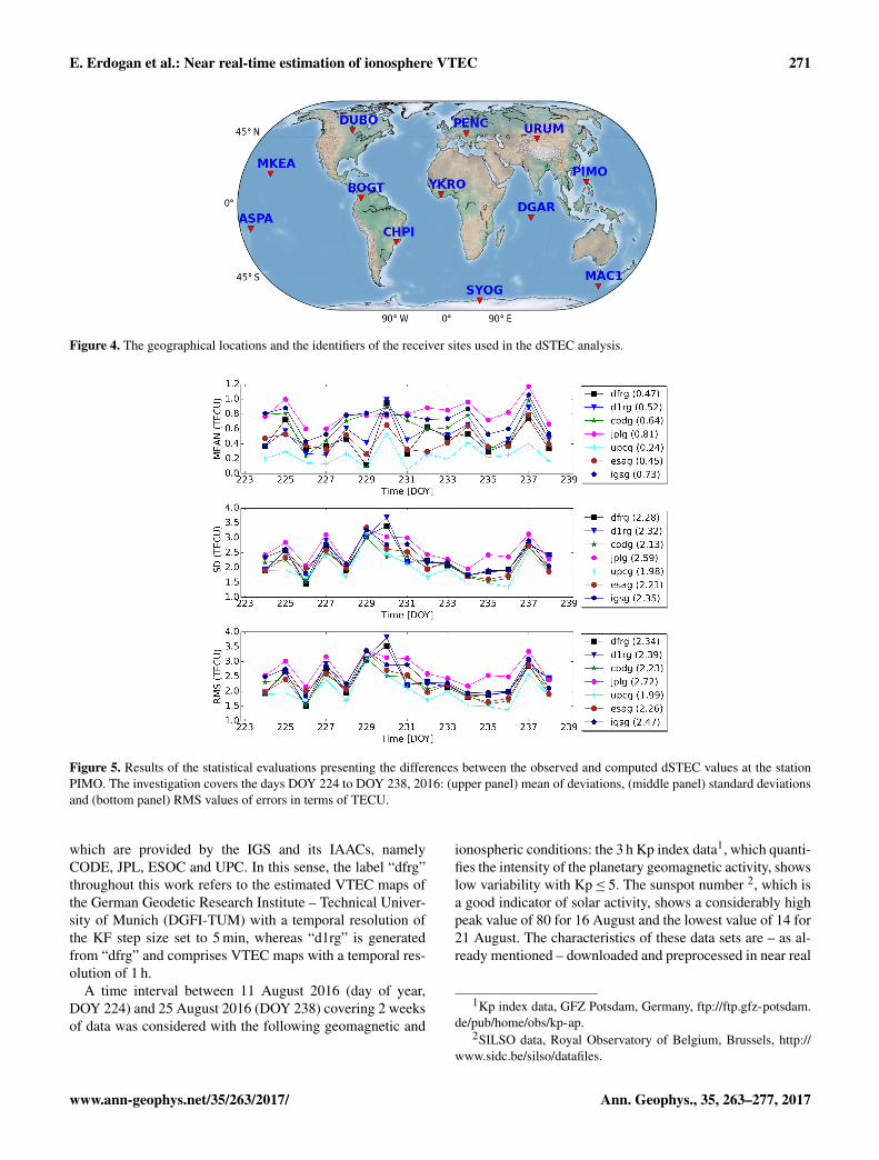
Figure 4. The geographical locations and the identifiers of the receiver sites used in the dSTEC analysis.

Figure 5. Results of the statistical evaluations presenting the differences between the observed and computed dSTEC values at the stationPIMO. The investigation covers the days DOY 224 to DOY 238, 2016: (upper panel) mean of deviations, (middle panel) standard deviationsand (bottom panel) RMS values of errors in terms of TECU.

which are provided by the IGS and its IAACs, namelyCODE, JPL, ESOC and UPC. In this sense, the label “dfrg”throughout this work refers to the estimated VTEC maps ofthe German Geodetic Research Institute – Technical Univer-sity of Munich (DGFI-TUM) with a temporal resolution ofthe KF step size set to 5 min, whereas “d1rg” is generatedfrom “dfrg” and comprises VTEC maps with a temporal res-olution of 1 h.

A time interval between 11 August 2016 (day of year,DOY 224) and 25 August 2016 (DOY 238) covering 2 weeksof data was considered with the following geomagnetic and

ionospheric conditions: the 3 h Kp index data1, which quanti-fies the intensity of the planetary geomagnetic activity, showslow variability with Kp≤ 5. The sunspot number 2, which isa good indicator of solar activity, shows a considerably highpeak value of 80 for 16 August and the lowest value of 14 for21 August. The characteristics of these data sets are – as al-ready mentioned – downloaded and preprocessed in near real

1Kp index data, GFZ Potsdam, Germany, ftp://ftp.gfz-potsdam.de/pub/home/obs/kp-ap.

2SILSO data, Royal Observatory of Belgium, Brussels, http://www.sidc.be/silso/datafiles.

www.ann-geophys.net/35/263/2017/ Ann. Geophys., 35, 263–277, 2017

272 E. Erdogan et al.: Near real-time estimation of ionosphere VTEC

time. The following subsections are dedicated to the resultsof these assessments.

6.1 Self-consistency analysis

The derivation of very accurate absolute STEC values fromGNSS measurements may be a challenging procedure sincethe observations include the DCBs of the receivers and thetransmitting satellites. Several research groups have providedGNSS-based solutions regarding the TEC modeling with ap-propriate approaches for quality assessment; for example,see Rovira-Garcia et al. (2015), Li et al. (2015), Bruniniet al. (2011) and Orus et al. (2007). In the context of qual-ity assessment, through a GPS phase-continuous arc, differ-ential STEC, i.e., dSTEC values, can be obtained with anaccuracy of less than 0.1 TECU (Feltens et al., 2011). Notethat 1 TECU is equivalent to 1016 electrons m−2. A test valuedSTECk for assessing the quality of the products at an epochk can be obtained by

dSTECk = dSTECobs,k − dSTECmap,k (31)

(Orus et al., 2007), where dSTECobs,k is the difference of theGPS geometry-free linear combination at the epoch k withanother linear combination computed on the same continu-ous arc at a reference epoch characterized by the highest el-evation angle. The computed dSTEC values from the VTECmaps denoted as dSTECmap,k at the same epoch k and thereference epoch are obtained by multiplying the VTEC val-ues with the elevation-dependent mapping function (Eq. 13).The geographical locations and the names of the receiverstations selected for the dSTEC evaluation are depicted inFig. 4. The test receivers are chosen globally and located atlow and high latitudes, which can reveal the VTEC modelaccuracy at the regions characterized by varying VTEC ac-tivity. The receivers at the sites MKEA, ASPA, BOGT, CHPI,YKRO, DGAR and PIMO are located at middle and low lat-itudes, whereas DUBO, PENC, URUM, SYOG and MAC1are established at higher latitudes. As an exemplified analy-sis, the mean, the standard deviation and the RMS values ofdaily dSTEC variations are computed using the data from theobservation site PIMO as presented in Fig. 5. The numberswithin the parentheses shown on the legends give the averagevalues of the corresponding statistical measures for the entiretest period, which are also summarized in Fig. 6. The biasesof the VTEC maps at the PIMO station show day-to-day vari-ations from 0.1 to 1.2 TECU. The average RMS errors of thedfrg and the d1rg solutions are 2.34 and 2.39 TECU, respec-tively, which are in close agreement with the RMS values ofthe analysis centers ranging from 1.99 to 2.72 TECU. Tak-ing into account the daily RMS variations plotted in Fig. 5,the VTEC solutions dfrg and d1rg show larger values only atDOY 230 but smaller deviations for the rest of the test period.

In Fig. 6, as a summary of statistical measures, the aver-age mean values and standard deviations as well as the av-erage RMS errors for the entire test period are visualized

for each of the 12 receiver sites and the seven VTEC mod-els. As is expected, the dSTEC error for the sites at low lat-itudes (ASPA, BOGT, YKRO, DGAR, PIMO) are generalhigher than those obtained at high latitudes. Especially, theASPA site has rather high errors for each of the VTEC mapsin terms of RMS error. The site is very close to the geo-magnetic equator, and it can suffer from poor nearby datacoverage due to its geographic location on an oceanic is-land. The result of our solution dfrg has an average bias of0.04 TECU. The biases with respect to the other maps varybetween −0.02 and 0.36 TECU. The average standard devi-ation for dfrg is 1.78 TECU, which shows a moderate accu-racy compared to those of the other maps, which range from1.66 to 1.96 TECU. The RMS error of dfrg has 1.81 TECU,whereas the RMS errors of the other VTEC solutions varybetween 1.70 and 2.00 TECU. A closer look into the aver-age RMS errors for each of the sites reveals that although thepresented approach shows a slightly higher deviation onlyfor the ASPA station, the accuracy at the remaining sitesis compatible with that of the analysis centers. Moreover,concerning the temporal resolution, the RMS error of dfrgamounts to 1.81 TECU and is thus slightly better than d1rgwith 1.85 TECU. However, during high solar activity, a con-siderable difference might be expected.

6.2 Validation by the Jason-2 altimetry

The dual-frequency altimeter onboard the Jason-2 satellitecan directly measure in the nadir direction using two differentfrequencies, which allow the extraction of VTEC data withless effort and without applying any mapping between STECand VTEC (Dettmering et al., 2011) according to Eq. (12).The VTECs provided by Jason-2 are taken into account asreference since they allow the evaluation of the errors of theglobal VTEC maps over the oceans as well as over regionsthat exhibit poor estimation quality due to the availability ofonly a few GNSS measurements. It should be noted that al-though the Jason-2 satellite provides accurate, direct and in-dependent VTEC data, several studies reported that the mea-surements are contaminated by an offset of around 3 TECUcompared to the GNSS-derived VTEC products (Tseng et al.,2010; Chen et al., 2016).

Before using the altimeter data for the comparisons, a me-dian filter with a window size of 20 s was applied to smooththe data. It is worth mentioning that Jason-2 radar altimetryprovides data with a higher spatial and temporal resolutioncompared to the VTEC maps. Therefore, a linear interpola-tion in the spatial and time domains was applied to obtainVTEC values for the corresponding time and location of thealtimetry observations. The interpolation is performed in theSun-fixed coordinate system between consecutive epochs.Figure 7 shows exemplified ground tracks of Jason-2 with theassociated VTEC values for the entire day of 16 August 2016(DOY 229). High VTEC variations around the equatorial re-

Ann. Geophys., 35, 263–277, 2017 www.ann-geophys.net/35/263/2017/

E. Erdogan et al.: Near real-time estimation of ionosphere VTEC 273

Figure 6. Results of the statistical evaluations presenting the differences between the observed and computed dSTEC values, which coverthe days between DOY 224 and DOY 238, 2016: (upper panel) mean of deviations, (middle panel) standard deviations and (bottom panel)RMS values of deviation in terms of TECU.

Figure 7. Ground tracks of the Jason-2 altimetry mission for 16 Au-gust 2016 (DOY 229). The colors show the magnitude of VTEC asacquired from the satellite measurement system.

Figure 8. Ground track of the Jason-2 altimetry satellite between00:00 and 01:00 UTC on DOY 229, 2016. The colors show the mag-nitude of VTEC in TECU acquired from the satellite.

Figure 9. VTEC values from the six analysis centers and Jason-2between 00:00 and 01:00 UTC on DOY 229, 2016 in TECU.

gions can be clearly seen. This day has the highest sun spotnumber during the test period.

For the sake of clarity, a selected data set between 00:00and 01:00 UTC from Fig. 7 is depicted in Fig. 8. The equa-torial ionization anomaly (EIA), which is characterized bytwo crests at both sides of the geomagnetic equator and atrough around the equator (Appleton, 1946), can be seen inFigs. 7 and 8 by carefully interpreting the colors along theground tracks. The VTEC values obtained from Jason-2 andthe seven VTEC maps, using the aforementioned interpo-lation method, are visualized in Fig. 9 for the ground trackdisplayed in Fig. 8. The camelback-shaped EIA in terms ofVTEC is illustrated by two regions, including the peak VTECvalues between 0.0 and 0.3 h of day (hod). The morphologyof the EIA defined by the Jason-2 VTEC is clearly repre-sented by the VTEC maps. The DGFI-TUM solutions arein good agreement with all the other VTEC values. For the

www.ann-geophys.net/35/263/2017/ Ann. Geophys., 35, 263–277, 2017

274 E. Erdogan et al.: Near real-time estimation of ionosphere VTEC

Figure 10. Comparison of VTEC values acquired from the analysis centers and the DGFI-TUM solutions with Jason-2 altimetry VTEC databetween DOY 224 and DOY 238, 2016; (upper panel) mean deviations, (middle panel) standard deviations and (bottom panel) RMS valuesof deviations in terms of TECU.

whole day, a mean bias of −1.23 TECU and a standard de-viation of 3.43 TECU is computed for the dfrg VTEC solu-tion. The results are compatible with the solution of the otherVTEC maps showing mean biases ranging from −1.77 to1.23 TECU and standard deviations from 2.06 to 4.74 TECU.

For the entire test period, the results of the comparisons interms of daily mean, standard deviation and RMS values aswell as their overall averaged values for the entire test periodare illustrated in Fig. 10. The average relative biases of theVTEC maps show variations between 0.5 and −2.0 TECU;our two solutions labeled as dfrg and d1rg both have an av-erage relative bias of −1.6 TECU. The daily standard devia-tions vary between 3.2 and 5.0 TECU; their averages deviatearound 4.0 TECU and are also in accordance with those de-rived from a recent comparison study by Hernández-Pajareset al. (2016) stating that the daily deviations for the resultsof the IAACs can vary from a few TECU to 10 TECU. Oursolutions have an average RMS error of 4.7 TECU, whichdoes not exceed that computed from the other analysis cen-ters ranging between 4.0 and 4.7 TECU. A detailed look intothe daily RMS values indicates that the estimated VTEC val-ues of our solutions are generally in good agreement with theresults of the analysis centers.

7 Conclusions and future improvements

A near real-time processing framework that is capable of au-tomated data downloading, data preprocessing, Kalman fil-

tering and formatted product generation is presented to pro-vide VTEC maps as well as satellite and receiver DCBs ofGPS and GLONASS in near real time. The B-spline repre-sentation of global VTEC is incorporated into the Kalmanfilter procedure. The filter was also extended to integrate theequality constraint equations comprising the spherical andDCB-related restrictions. Coefficients of the B-spline modeland the DCBs, which constitute the unknown parameters, arerecursively estimated by exploiting hourly GNSS observa-tions acquired from the IGS data centers with 1 h latency.The ionosphere observable is derived from raw GNSS codeand phase measurements using the geometry-free linear com-binations.

The validation of the proposed approach is carried outusing GNSS data downloaded in near real time coveringa time span of 2 weeks. To summarize, according to theself-consistency analysis, an RMS value of 1.81 TECU wasfound. The four IAACs, CODE, JPL, ESOC and UPC, aswell as the IGS combination product exhibit comparableRMS errors between 1.70 and 2.00 TECU. Moreover, theJason-2 validation shows that the RMS error achieved bythe proposed method fits well with the results of the IAACs.Considering the comparisons, specific to the test period itmight be concluded that the estimated VTEC products usingthe presented near real-time strategy shows promising initialresults in terms of accuracy and overall agreement with thepost-processed final products of IGS and its analysis centers,which are publicly available with several days of latency.

Ann. Geophys., 35, 263–277, 2017 www.ann-geophys.net/35/263/2017/

E. Erdogan et al.: Near real-time estimation of ionosphere VTEC 275

Furthermore, the results encourage further research to im-prove the presented model as mentioned below.

One drawback associated with the KF is the requirementof the complete knowledge of the prior information, i.e., theprocess noise covariance matrix 6w, and the covariance ma-trix 6y of the measurement errors have to be given. Thecommon practice of selecting these matrices manually is con-ducted by doing tests through multiple runs of the filter fordifferent values of these parameters (Maybeck, 1979). How-ever, the test data may not be adequate for properly defin-ing these matrices beforehand or they can vary unpredictablythroughout the time period (Brown and Hwang, 2012). If theprior information is not appropriate, the filter is no longeroptimal and can result in an estimation of poor quality, oreven worse, the filter may diverge. To cope with such sit-uations in ionosphere modeling, the implemented approachwill be extended by adaptive methods to estimate the covari-ance matrices in run time as a further improvement. More-over, the evaluations presented here show that the developedapproach exhibits promising results during a period of quietsolar activity, but further tests have to be conducted usingGNSS data sets covering a long time span and downloadedin near real time during time periods of high solar activityand solar events, e.g., solar flares and coronal mass ejections.

8 Data availability

The global VTEC maps in IONEX format used in the com-parisons were acquired from the Crustal Dynamics Data In-formation System (CDDIS) data center by the followingFTP server: ftp://cddis.gsfc.nasa.gov/gnss/products/ionex/.The data of the Jason-2 altimetry mission are available via theFTP server: ftp://data.nodc.noaa.gov/pub/data.nodc/jason2/ogdr/ogdr/. The hourly available GNSS data from IGS siteswere operationally downloaded in real time through mir-roring to the different IGS data centers, i.e., the CDDIS(ftp://cddis.gsfc.nasa.gov/pub/gps/data/hourly/), the Bunde-samt für Kartographie und Geodäsie (BKG) (ftp://igs.bkg.bund.de/IGS/nrt/), the Institut Geographique National (IGN)(ftp://igs.ensg.ign.fr/pub/igs/data/hourly) and the Korean As-tronomy and Space Science Institute (KASI) (ftp://nfs.kasi.re.kr/). Furthermore, ultrarapid orbits of GPS and GLONASSsatellites utilized in the data preprocessing step can be ac-cessed through FTP servers, namely for GPS via ftp://cddis.gsfc.nasa.gov/pub/gps/products and for GLONASS via ftp://ftp.glonass-iac.ru/MCC/PRODUCTS/.

Competing interests. The authors declare that they have no conflictof interest.

Acknowledgements. The authors would like to thank the follow-ing services and institutions for providing the input data: IGS andits data centers, the Center for Orbit Determination in Europe(CODE, University of Berne, Switzerland), the Jet Propulsion Lab-oratory (JPL, Pasadena,California, USA), the European Space Op-erations Centre of European Space Agency (ESOC, Darmstadt, Ger-many) and the Universitat Politècnica de Catalunya/IonSAT (UPC,Barcelona, Spain).

This work was supported by the German Research Foundation(DFG) and the Technical University of Munich (TUM) in the frame-work of the Open Access Publishing Program. Moreover, the pre-sented models were developed in the frame of the project “Devel-opment of a novel adaptive model to represent global ionosphereinformation from combining space geodetic measurement systems”(ADAPIO) (German title: “Entwicklung eines neuartigen adaptivenModells zur Darstellung von globalen Ionosphäreninformationenaus der Kombination geodätischer Raumverfahren”), which wasfunded by the German Federal Ministry for Economic Affairs andEnergy via the German Aerospace Center (DLR, Bonn, Germany).

The topical editor, K. Hosokawa, thanks the two anonymousreferees for help in evaluating this paper.

References

Anghel, A., Carrano, C., Komjathy, A., Astilean, A., and Letia, T.:Kalman filter-based algorithms for monitoring the ionosphereand plasmasphere with GPS in near-real time, J. Atmos. Sol.-Terr. Phys., 71, 158–174, doi:10.1016/j.jastp.2008.10.006, 2009.

Appleton, E. V.: Two Anomalies in the Ionosphere, Nature, 157,691–691, doi:10.1038/157691a0, 1946.

Brown, R. G. and Hwang, P. Y. C.: Introduction to Random Signalsand Applied Kalman Filtering: with MATLAB exercises, JohnWiley & Sons, Inc., USA, 4th Edn., 2012.

Brunini, C., Camilion, E., and Azpilicueta, F.: Simulationstudy of the influence of the ionospheric layer height inthe thin layer ionospheric model, J. Geodesy, 85, 637–645,doi:10.1007/s00190-011-0470-2, 2011.

Chen, P., Yao, Y., and Yao, W.: Global ionosphere maps based onGNSS, satellite altimetry, radio occultation and DORIS, GPS So-lutions, 1–12, doi:10.1007/s10291-016-0554-9, 2016.

Ciraolo, L., Azpilicueta, F., Brunini, C., Meza, A., and Radicella,S. M.: Calibration errors on experimental slant total electroncontent (TEC) determined with GPS, J. Geodesy, 81, 111–120,doi:10.1007/s00190-006-0093-1, 2007.

Dach, R., Hugentobler, U., Fridez, P., and Meindl, M.: BerneseGPS Software Version 5.0, Astronomical Institute, Universityof Bern, Staempfli Publications AG, available at: http://www.bernese.unibe.ch/docs50/DOCU50.pdf (last access: 18 Febru-ary 2017), 2007.

Dettmering, D., Schmidt, M., Heinkelmann, R., and Seitz,M.: Combination of different space-geodetic observationsfor regional ionosphere modeling, J. Geodesy, 85, 989–998,doi:10.1007/s00190-010-0423-1, 2011.

www.ann-geophys.net/35/263/2017/ Ann. Geophys., 35, 263–277, 2017

276 E. Erdogan et al.: Near real-time estimation of ionosphere VTEC

Durmaz, M. and Karslioglu, M. O.: Regional vertical total electroncontent (VTEC) modeling together with satellite and receiver dif-ferential code biases (DCBs) using semi-parametric multivari-ate adaptive regression B-splines (SP-BMARS), J. Geodesy, 89,347–360, doi:10.1007/s00190-014-0779-8, 2015.

Durmaz, M., Karslioglu, M. O., and Nohutcu, M.: Regional VTECmodeling with multivariate adaptive regression splines, Adv.Space Res., 46, RS0D12, doi:10.1016/j.asr.2010.02.030, 2010.

Feltens, J., Angling, M., Jackson-Booth, N., Jakowski, N., Hoque,M., Hernández-Pajares, M., Aragón-Àngel, A., Orús, R., andZandbergen, R.: Comparative testing of four ionospheric mod-els driven with GPS measurements, Radio Sci., 46, RS0D12,doi:10.1029/2010RS004584, 2011.

Fu, L.-L. and Cazenave, A. (Eds.): Satellite Altimetry and Earth Sci-ences A Handbook of Techniques and Applications, AcademicPress Inc., San Diego, California, 2001.

Gao, Y., Zhang, Y., and Chen, K.: Development of a realtime single-frequency Precise Point Positioning system and test results, in:Proceedings of the 19th International Technical Meeting of theSatellite Division of The Institute of Navigation (ION GNSS2006), 2297–2303, Fort Worth, TX, 2006.

Gelb, A. (Ed.): Applied Optimal Estimation, The MIT Press, Cam-bridge, 1974.

Grewal, M. S. and Andrews, A. P.: Kalman Filtering: Theory andPractice Using MATLAB, John Wiley & Sons, Inc., 3rd Edn.,Hoboken, New Jersey, 2008.

Heelis, R. A.: Aspects of Coupling Processes in the Ionosphere andThermosphere, in: Modeling the Ionosphere-Thermosphere Sys-tem, 161–169, doi:10.1002/9781118704417.ch14, John Wiley &Sons, Ltd, 2014.

Hernández-Pajares, M., Juan, J., and Sanz, J.: New approaches inglobal ionospheric determination using ground GPS data, J. At-mos. Sol.-Terr. Phys., 61, 1237–1247, 1999.

Hernández-Pajares, M., Juan, J. M., Sanz, J., Aragón-Àngel, À.,García-Rigo, A., Salazar, D., and Escudero, M.: The ionosphere:Effects, GPS modeling and the benefits for space geodetic tech-niques, J. Geodesy, 85, 887–907, doi:10.1007/s00190-011-0508-5, 2011.

Hernández-Pajares, M., Roma-Dollase, D., Krankowski, A.,Ghoddousi-Fard, R., Yuan, Y., Li, Z., Zhang, H., Shi, C., Fel-tens, J., Komjathy, A., Vergados, P., Schaer, S., Garcia-Rigo, A.,and Gómez-Cama, J. M.: Comparing performances of seven dif-ferent global VTEC ionospheric models in the IGS context, in:International GNSS Service Workshop 2016, Sydney, Australia,2016.

Jee, G., Burns, A. G., Wang, W., Solomon, S. C., Schunk, R. W.,Scherliess, L., Thompson, D. C., Sojka, J. J., Zhu, L., and Scher-liess, L.: Driving the TING Model with GAIM Electron Densi-ties: Ionospheric Effects on the Thermosphere, J. Geophys. Res.-Space, 113, A03305, doi:10.1029/2007JA012580, 2008.

Kalman, R.: A new approach to linear filtering and prediction prob-lems, Journal of Basic Engineering, 82, 35–45, 1960.

Komjathy, A.: Global ionospheric total electron content mappingusing the Global Positioning System, PhD thesis, Universityof New Brunswick, available at: http://www2.unb.ca/gge/Pubs/TR188.pdf (last access: 12 February 2017), 1997.

Komjathy, A. and Langley, R.: An assessment of predicted and mea-sured ionospheric total electron content using a regional GPS net-

work, in: Proceedings of the 1996 National Technical Meeting ofThe Institute of Navigation, 615–624, Santa Monica, CA, 1996.

Le, A., Tiberius, C., van der Marel, H., and Jakowski, N.: Useof Global and Regional Ionosphere Maps for Single-FrequencyPrecise Point Positioning, in: Observing our Changing Earth,edited by: Sideris, M. G., 759–769, doi:10.1007/978-3-540-85426-5_87, Springer Berlin Heidelberg, 2009.

Lee, I. T., Matsuo, T., Richmond, A. D., Liu, J. Y., Wang, W.,Lin, C. H., Anderson, J. L., and Chen, M. Q.: Assimilation ofFORMOSAT-3/COSMIC electron density profiles into a coupledthermosphere/ionosphere model using ensemble Kalman filter-ing, J. Geophys. Res., 117, A10318, doi:10.1029/2012JA017700,2012.

Li, Z., Yuan, Y., Wang, N., Hernandez-Pajares, M., and Huo, X.:SHPTS: towards a new method for generating precise globalionospheric TEC map based on spherical harmonic and gener-alized trigonometric series functions, J. Geodesy, 89, 331–345,doi:10.1007/s00190-014-0778-9, 2015.

Limberger, M.: Ionosphere modeling from GPS radio occultationsand complementary data based on B-splines, PhD thesis,Technischen Universität München, http://nbn-resolving.de/urn/resolver.pl?urn:nbn:de:bvb:91-diss-20151006-1254715-1-1(last access: 12 February 2017), 2015.

Limberger, M., Liang, W., Schmidt, M., Dettmering, D., andHugentobler, U.: Regional representation of F2 Chapman pa-rameters based on electron density profiles, Ann. Geophys., 31,2215–2227, doi:10.5194/angeo-31-2215-2013, 2013.

Liu, J. Y., Chuo, Y. J., Shan, S. J., Tsai, Y. B., Chen, Y. I., Pulinets,S. A., and Yu, S. B.: Pre-earthquake ionospheric anomalies reg-istered by continuous GPS TEC measurements, Ann. Geophys.,22, 1585–1593, doi:10.5194/angeo-22-1585-2004, 2004.

Liu, Z.: Ionosphere Tomographic Modeling and Applications Us-ing Global Positioning System (GPS) Measurements, PhD the-sis, University of Calgary, available at: http://www.ucalgary.ca/engo_webdocs/YG/04.20198.Zhizhao_Liu.pdf (last access:12 February 2017), 2004.

Mannucci, A. J., Wilson, B. D., Yuan, D. N., Ho, C. H., Lindqwister,U. J., and Runge, T. F.: A global mapping technique for GPS-derived ionospheric total electron content measurements, RadioSci., 33, 565–582, doi:10.1029/97RS02707, 1998.

Maybeck, P. S.: Stochastic Models, Estimation and Control VolumeI, Academic Press, New York, NY, 1979.

Mitchell, C. N. and Spencer, P. S. J.: A three-dimensional time-dependent algorithm for ionospheric imaging using GPS, Annalsof Geophysics, 46, 687–696, doi:10.4401/ag-4373, 2003.

Monte-Moreno, E. and Hernández-Pajares, M.: Occurrence of solarflares viewed with GPS: Statistics and fractal nature, J. Geophys.Res.-Space, 119, 9216–9227, doi:10.1002/2014JA020206, 2014.

Orus, R., Cander, L. R., and Hernandez-Pajares, M.: Testing re-gional vertical total electron content maps over Europe duringthe 17–21 January 2005 sudden space weather event, Radio Sci.,42, RS3004, doi:10.1029/2006RS003515, 2007.

Rovira-Garcia, A., Juan, J. M., Sanz, J., and Gonzalez-Casado,G.: A Worldwide Ionospheric Model for Fast Precise PointPositioning, IEEE T. Geosci. Remote Sens., 53, 4596–4604,doi:10.1109/TGRS.2015.2402598, 2015.

Schaer, S.: Mapping and Predicting the Earth’s Ionosphere Usingthe Global Positioning System, PhD thesis, University of Bern,Bern, 1999.

Ann. Geophys., 35, 263–277, 2017 www.ann-geophys.net/35/263/2017/

E. Erdogan et al.: Near real-time estimation of ionosphere VTEC 277

Scherliess, L., Schunk, R. W., Sojka, J. J., Thompson, D. C., andZhu, L.: Utah State University Global Assimilation of Iono-spheric Measurements Gauss-Markov Kalman filter model of theionosphere: Model description and validation, J. Geophys. Res.,111, A11315, doi:10.1029/2006JA011712, 2006.

Schmidt, M.: Wavelet modelling in support of IRI, Adv. Space Res.,39, 932–940, doi:10.1016/j.asr.2006.09.030, 2007.

Schmidt, M., Bilitza, D., Shum, C., and Zeilhofer, C.: Regional 4-Dmodeling of the ionospheric electron density, Adv. Space Res.,42, 782–790, doi:10.1016/j.asr.2007.02.050, 2008.

Schmidt, M., Dettmering, D., Mößmer, M., Wang, Y., and Zhang,J.: Comparison of spherical harmonic and B spline models forthe vertical total electron content, Radio Sci., 46, RS0D11,doi:10.1029/2010RS004609, 2011.

Schmidt, M., Dettmering, D., and Seitz, F.: Using B-Spline Expan-sions for Ionosphere Modeling, in: Handbook of Geomathemat-ics, edited by: Freeden, W., Nashed, M. Z., and Sonar, T., 939–983, doi:10.1007/978-3-642-54551-1_80, Springer Berlin Hei-delberg, Berlin, Heidelberg, 2015.

Schumaker, L. L. and Traas, C.: Fitting scattered data on spherelikesurfaces using tensor products of trigonometric and polynomialsplines, Numer. Math., 60, 133–144, doi:10.1007/BF01385718,1991.

Schunk, R. W. and Nagy, A. F.: Ionosphere: Physics, PlasmaPhysics, and Chemistry, Cambridge University Press, New York,2nd Edn., 2009.

Schunk, R. W., Scherliess, L., Sojka, J. J., Thompson, D. C., An-derson, D. N., Codrescu, M., Minter, C., Fuller-Rowell, T. J.,Heelis, R. A., Hairston, M., and Howe, B. M.: Global Assim-ilation of Ionospheric Measurements (GAIM), Radio Sci., 39,RS1S02, doi:10.1029/2002RS002794, 2004.

Simon, D.: Kalman filtering with state equality constraints, IEEE T.Aero. Elec. Sys., 38, 128–136, doi:10.1109/7.993234, 2002.

Simon, D.: Optimal State Estimation, doi:10.1088/1741-2560/2/3/S07, John Wiley & Sons, Inc., Hoboken, NewJersey, 2006.

Simon, D.: Kalman filtering with state constraints: a survey of linearand nonlinear algorithms, IET Control Theory & Applications, 4,1303–1318, doi:10.1049/iet-cta.2009.0032, 2010.

Skone, S.: Wide area ionosphere grid modelling in the auro-ral region, PhD thesis, University of Calgary, available at:http://sirsi1.lib.ucalgary.ca/uhtbin/cgisirsi/0/0/0/5?library=UCALGARY-S&searchdata1=%5EC2619212 (last access:12 February 2017), 1999.

Tseng, K.-H., Shum, C. K., Yi, Y., Dai, C., Lee, H., Bilitza, D.,Komjathy, A., Kuo, C. Y., Ping, J., and Schmidt, M.: RegionalValidation of Jason-2 Dual-Frequency Ionosphere Delays, Mar.Geodesy, 33, 272–284, doi:10.1080/01490419.2010.487801,2010.

Wang, C., Rosen, I. G., Tsurutani, B. T., Verkhoglyadova, O. P.,Meng, X., and Mannucci, A. J.: Statistical characterization ofionosphere anomalies and their relationship to space weatherevents, Journal of Space Weather and Space Climate, 6, A5,doi:10.1051/swsc/2015046, 2016.

Wang, N., Yuan, Y., Li, Z., Montenbruck, O., and Tan, B.: Determi-nation of differential code biases with multi-GNSS observations,J. Geodesy, 90, 209–228, doi:10.1007/s00190-015-0867-4, 2015.

Yang, Y.: Adaptively Robust Kalman Filters with Applications inNavigation, in: Sciences of Geodesy – I, edited by: Xu, G., 49–82, doi:10.1007/978-3-642-11741-1_2, Springer Berlin Heidel-berg, Berlin, Heidelberg, 2010.

Zeilhofer, C.: Multi-dimensional B-spline Modeling of Spatio-temporal Ionospheric Signals, Tech. Rep. 123, DeutscheGeodätische Kommission, München, 2008.

Zeilhofer, C., Schmidt, M., Bilitza, D., and Shum, C.: Re-gional 4-D modeling of the ionospheric electron density fromsatellite data and IRI, Adv. Space Res., 43, 1669–1675,doi:10.1016/j.asr.2008.09.033, 2009.

www.ann-geophys.net/35/263/2017/ Ann. Geophys., 35, 263–277, 2017