1

REGIONAL FDI SPILLOVERS AND PRODUCTIVITY OF LOCAL FIRMS

IN NEW EU MEMBER STATES

Nebojša Stojčić1 and Edvard Orlić2

1University of Dubrovnik, Department of Economics and Business Economics, Lapadska Obala 7, 2000 Dubrovnik, Croatia (e-mail: nstojcic@unidu.hr) – corresponding author 2Edvard Orlić, Staffordshire University Business School, Leek Rd, ST4 2DF, Stoke-On-Trent, United Kingdom. (e-mail: Edvard.Orlić@staffs.ac.uk) Abstract. This research investigates how FDI affects the TFP of local firms in 59 NUTS3 regions of five new EU member states in 2004-2009 period. Although a lot of empirical work has been undertaken on the impact of FDI on indigenous firms’ performance the regional channels through which MNCs affect TFP of local firms have been investigated to a much lesser extent. The results from spatial Durbin model and several other analytical methods reveal existence of inter-regional TFP spillovers as well as intra-regional and horizontal inter-regional FDI spillovers. The inter-regional impact of independent variables on the TFP of local firms amounts to about half of the impact on the region itself. Keywords: FDI, TFP, regions, spatial analysis, new EU member states JEL: F23, R12

2

1. Introduction

The achievement of harmonious and balanced development of economic activities and

convergence of economic performance are among founding principles of European Union.

Yet, recent Report on economic and social cohesion in European Union (European

Commission, 2013) reveals widening of development gap between EU regions. This is

particularly true for regions in new EU member states whose GDP per capita falls below

EU27 average with ten least advanced EU regions coming from these countries. Many

theoretical models and empirical studies nowadays suggest that the persistence and widening

of regional development disparities can be attributed to differences in productivity caused by

variations in factor rewards, knowledge and technology intensity as well as spatial clustering

of industries (Esteban, 2000; Boldrin and Canova, 2001; Benito and Ezcurra, 2005). Same

line of reasoning indicates that one of the most important mechanisms behind regional

economic convergence is the diffusion of technology and knowledge.

A lot of attention in recent years has been devoted to the impact of foreign direct investment

(FDI) spillovers on the reduction of inter-regional income differences as well as the

convergence in the inter-sectoral and inter-regional reallocation of productive factors (De la

Fuente, 2002). The benefits of multinational corporations (MNCs) for local firms encompass

increased local demand for upstream industries and local supply within same industries as

well as forward linkages such as increased variety and quantity served at lower price

(Markusen and Venables, 1999; Lin and Saggi, 2007). Transition literature has so far

associated the entry of MNCs with enterprise restructuring (Djankov and Murrell, 2002),

export competitiveness (Rugraff, 2006) and productivity growth (Schadler et al., 2006).

Moreover, FDI spillovers influence regional output levels through technological spillovers

and vertical linkages (Altomonte and Guagliano, 2004). Yet, there is no evident role in

reducing the disparities across regions.

3

The high per capita FDI inflow in these countries makes it of crucial importance to analyse

whether incentives given to MNCs so far are warranted and should countries continue to

pursue policies aimed at attracting MNCs. To this end, the research posits two questions.

First, whether and up to what extent the regional disparities in these countries are emphasized

and second, whether MNCs contributed to regional convergence or divergence? In order to

answer these questions the influence of FDI spillovers on the regional productivity of

domestic firms in five new EU member states (Czech Republic, Estonia, Hungary, Slovak

Republic and Slovenia) in 2004-2009 period is examined.

The empirical analysis of paper consists of two building blocks. The decomposition of

regional income dynamics following Altomonte and Colantone (2008) is undertaken in order

to assess the role of productivity dynamics in reduction of regional economic imbalances.

Furthermore, a spatial Durbin model is applied to the data taken from Amadeus database in

order to investigate the role of FDI spillovers and number of other regional characteristics for

total factor productivity of domestic firms within regions defined at NUTS3 level. The

novelty of our approach lies in distinction between the impact of inter-regional productivity

spillovers among domestic firms, intra-regional and inter-regional FDI spillovers using spatial

econometric techniques. To the best of our knowledge, there has been no attempt to analyse

the role of FDI spillovers in regional productivity dynamics in such framework.

The rest of paper is structured as follows. Section two discusses different theoretical

perspectives on sources and the nature of regional variations in productivity. The patterns of

FDI spillovers are analysed in section three while section four assesses existing literature on

FDI and productivity. Regional differences in productivity are examined in section five. The

model of investigation relating productivity and FDI spillovers is discussed in section six. The

dataset is presented in section seven while results of econometric analysis of the relationship

4

between FDI spillovers and productivity of domestic firms are presented in section eight.

Finally, section nine concludes.

2. Theoretical foundations of regional productivity differences

Regional variations in productivity have been investigated within variety of economic schools

such as new classical, endogenous growth and more recently new economic geography

(NEG). The search for causes of regional economic disparities has pointed to number of

factors that could be behind divergent economic performance of regions ranging from

institutional factors, regional and industry characteristics to the behaviour of firms. While

diverging on opinions about origins and persistence of regional economic imbalances all

theories agree that important role in the process of convergence belongs to the diffusion of

technology and knowledge through spillover mechanisms.

New classical models consider regional variations in productivity as a temporary consequence

of differences in capital-labour ratios and technological progress (Barro and Sala-I-Martin,

1991; Gardiner et al., 2004; Altomonte and Colantone, 2008). In the world of perfect

competition, constant returns to scale, complete information and full divisibility of factors, the

diffusion of technology across market takes place freely and instantaneously irrespective of

regional or national administrative borders and paves the way for regional productivity

convergence. Findings from empirical studies, however, point to the persistence national and

regional income and productivity disparities more in line with predictions of endogenous

growth literature or new economic geography (Quah, 1996; De la Fuente, 2002; Altomonte

and Colantone, 2008).

Endogenous growth models suggest that the diffusion of technology across market does not

take place instantaneously and inter-regional productivity differences may persist and even

widen over time. This literature associates regional variations in productivity with

5

components of regional innovation potential such as knowledge base, technological intensity

of industries and proportion of workforce in knowledge intensive activities (Romer, 1986;

1990; Aghion and Howitt, 1998). The leadership of some regions in innovativeness provides

their firms and industries with competitive advantage on goods and services market (Gardiner

et al., 2004) and attracts inflow of knowledge and highly skilled workers from other regions

(Aumayr, 2007). This is the reason why the knowledge and technology diffusion potential

decreases with distance and above-average returns and knowledge externalities tend to be

geographically concentrated.

New economic geography models (NEG) associate localised increasing returns with spatial

concentration of economic activity and related externalities such as accumulation of skilled

labour, local knowledge spillovers, specialised suppliers and services, cooperation between

firms and scientific institutions as well as professional agencies (Krugman, 1991; Fujita et al.,

1999; Fujita and Thisse, 2003; Baldwin et al., 2005; Hafner, 2013; Stojcic, et al., 2013). The

emergence of agglomerations on particular locations is viewed as an outcome of socio-

cultural, political and institutional structures. These factors explain why regions with initially

similar underlying structures endogenously differentiate into rich “core” regions and less

wealthy “peripheral” regions (Ottaviano and Puga, 1998; Altomonte and Colantone, 2008).

Same factors can be accountable for the persistent inter-regional productivity differences.

3. FDI spillovers and productivity dynamics

Positive externalities of FDI in host country range from job creation, provision of necessary

capital, tax revenues to the productivity growth. The productivity spillovers are often labelled

as the most important benefits of FDI. According to Narula and Marin (2005), entry and

presence of MNCs generate efficiency gains for host country’s local firms and opens up the

possibility for them to access foreign markets via the marketing and business networks of

foreign companies with which they interact. This process, however, is not automatic but it

6

depends on the ability of local environment to absorb the benefits of MNCs presence.

Common classification of spillovers in the literature is the one on horizontal or intra-industry

spillovers and vertical or inter-industry spillovers which can be further divided on backward

and forward linkages indicating knowledge spillovers in supply chain.

Several theoretical models have been put forward explaining the mechanism of horizontal

spillovers. In one set of models the emphasis is on acquisition of information about the costs

and benefits of new methods, management practices and marketing strategies through

demonstration or imitation of MNCs activities (Wang and Blomstrom, 1992). Models of

competition spillovers generally assume that entry of MNCs motivates local firms to enforce

stricter or more cost conscious management and stimulate faster adoption of new technologies

and management practices (Blomstrom and Kokko, 1998). While on overall increased

competition provides incentives for domestic firms to improve their performance, in the short

run it may reduce market share of less productive firms and lead to their exit (Aitken and

Harrison, 1999). Finally, models of worker mobility postulate that MNCs provide host

country workforce with a higher degree of training, education and valuable working

experience which gets diffused to local firms through movement of trained workers (Smeets,

2008; Markusen and Trofimenko, 2009).

MNCs also have the incentive to improve the productivity of their suppliers (backward

linkages) through provision of training, organization and management, setting up a production

facility, technical support for the improvement of the quality of goods and inventory

management (Lall, 1980; Javorcik, 2004). Furthermore, forward linkages promote the forward

transfer of knowledge from MNCs in upstream sectors to downstream indigenous firms. By

purchasing high-quality intermediate products from MNCs domestic firms can improve their

efficiency and as in case with backward linkages domestic firm has to improve its product,

train its employees to use these more advanced technologies.

7

In one set of vertical spillovers models the entry of MNC increases demand for intermediate

inputs which establishes the backward linkage (Rodriguez-Clare, 1996). According to

Markusen and Venables (1999) entry of MNC produces competitive effect in the final goods

sector, leading to exit of domestic firms. At the same time, establishment of backward

linkages leads to lower average costs and increase in profits resulting in increased entry in

upstream sector. This entry causes third effect as the reduction in prices of inputs benefits

firms in downstream sector because of improved and cheaper intermediate products supplied

by domestic firms. Finally, Pack and Saggi (2001) show how technology transfer to firms in

upstream sector induces entry of other suppliers thus reducing concentration and lowering

prices.

The necessary condition for transformation of knowledge spillovers potential into actual

knowledge spillovers is the existence of absorptive capacity. On the one hand, it is suggested

that the potential for technological imitation and adoption is larger when the technology gap

between countries is wider (Findlay, 1978). However, Glass and Saggi (1998) suggest that it

is less likely for domestic firms to have the human capital, organisational capabilities and

sources of finance, physical infrastructure and distribution networks to benefit from spillovers

when the technological gap is large. Cohen and Levinthal (1990) relate firm’s absorptive

capacity with its existing level of technological competence at the time of foreign entry as

well as the learning and investment efforts it makes afterwards in order to benefit from

foreign knowledge.

The possibilities for indigenous firms to benefit from knowledge spillovers of MNCs located

nearby are also affected by geographical distance. As knowledge is mainly tacit, geographical

distance inhibits its transmission and absorption. Therefore, spatial proximity facilitates the

process of knowledge diffusion influencing the existence and magnitude of spillovers for both

domestic firms and MNCs with asset seeking motives. According to Girma (2005)

8

demonstration effects will be local as the benefits are likely to be spread to neighbouring

firms while the low mobility of labour can be a strong obstacle for technology spillovers.

Finally, MNCs may prefer local linkage industries in order to minimize transaction costs and

facilitate communication with the domestic supplier or distributor.

4. Review of literature

Early research on FDI spillovers has related measures of labour productivity with the share of

foreign presence using aggregated data limited to a very short time span (Caves, 1974;

Globerman, 1979; Blomstrom and Persson, 1983; Blomstrom, 1986). Second generation of

empirical studies used firm level panel data and included many factors not considered earlier

such as industry and regional characteristics and firm-level specificities. It also addressed

methodological problems of the previous literature such as bias of total factor productivity

arising from the fact that a firm may observe part of its productivity before the choice of

inputs is made (Olley and Pakes, 1996; Levinsohn and Petrin, 2003). Existing studies have

generally reported ambiguous results on the impact of FDI horizontal spillovers while

theoretical predictions about positive impact of vertical spillovers have largely been

confirmed (Javorcik, 2004; Tytell and Yudayeva, 2005; Gorodnichenko et al., 2007; Blalock

and Gertler, 2008; Lefilleur and Maurel, 2010; Havranek and Irsova, 2011).

Over recent years sizeable body of empirical literature has addressed the spatial dimension of

FDI knowledge spillovers. Liu and Wei (2006) found evidence of strong regional intra

industry and inter industry spillovers from FDI and R&D on productivity in China while

inter-regional spillovers are mostly negative due to barriers to the movement of factors of

production and output across regions. Lin and Kwan (2013) show that FDI generates negative

intra-regional spillovers to domestic firms. However, local firms are found to benefit from

inter-regional FDI spillovers. Same study reports that in the long run the positive inter-

9

regional spillovers outweigh the negative intra-regional spillovers thus creating overall

positive effect.

Findings from European countries are somewhat opposite. Using UK data, Driffield (2004)

showed that there are positive productivity spillovers from FDI in the same region while FDI

outside the region has a negative impact on productivity. Girma and Wakelin (2007) assess

whether the benefits from FDI are particularly high or low in relatively underdeveloped

regions. Their results indicate that the productivity within and across sectors is positively

affected by FDI within but not outside the region. Furthermore, they report evidence that

domestic plants located in regions where MNCs receive government assistance gain less from

FDI. Smaller plants are found to benefit more from FDI, especially those with a relatively

high proportion of skilled employees accentuating the role of absorptive capacity.

Regional aspect of FDI might be particularly important in new EU member states. In these

countries FDI was mainly attracted to capital cities and western regions (Torlak, 2004), thus

the absence or negative effects of FDI spillovers on national level in transition economies

may be offset by positive effects on regional level which so far have received less attention.

Empirical analysis of regional patterns of spillovers in transition economies has been

conducted by several authors. Nicolini et al. (2007) used spatial error model taking into

account both spatial dependence and spatial heterogeneity on the sample of manufacturing

firms operating in Bulgaria, Poland and Romania between 1998 and 2003. Their findings

reveal positive and significant intra and inter industry spillovers at regional level. Negative

spillovers are found outside the region though limited to specific groups of regions, such as

the capital regions and regions bordering with former EU-15 countries. Large firms in regions

with high absorptive capacity enjoy higher total factor productivity growth rates.

Evidence from Altomonte and Colantone (2008) for Romania suggests that in case of regional

disparities MNEs act as magnifiers of these disparities instead of being factor of convergence.

10

The entry of MNEs in selected regions leads to compositional effect associated with the better

performance of these firms with respect to domestic ones and tends to magnify disparities.

Moreover, the restructuring efforts of MNEs demonstrate great deal of heterogeneity leading

to variations in output dynamics across regions and further divergence. Positive spillover

effects of MNEs on domestic firms are found in best performing areas while in laggard

regions MNEs crowd out domestic firms.

There are also studies that failed to confirm the importance of regional spillovers. Halpern and

Murakozy (2007) examined productivity spillovers in Hungary for the period 1996-2003 and

weighed measures of horizontal and vertical spillovers by distance expecting that the farther

the foreign firm, the smaller the spillover. They found that both types of spillovers within or

across regions were not different from each other. Using an unbalanced panel of firms in five

transition countries (Hungary, Poland, Romania, Bulgaria and Czech Republic) Torlak (2004)

found evidence for productivity spillovers for the Czech Republic and Poland. Yet, when

controlling for location-specific variations in productivity due to agglomeration economies or

other region-specific effects positive result only remains in the case of Czech Republic whilst

a negative effect is detected in the Bulgarian case.

5. Micro-foundations of regional productivity dynamics

Several authors over recent years have suggested that the sources of variations in aggregate

productivity should be looked for within plant changes in productivity related to technology

diffusion as well as in between plant changes in the allocation of inputs and in the effect of

entry and exit of firms. (Bartelsmann et al., 2004; Altomonte and Colantone, 2008; Resmini

and Nicolini, 2011). The starting point in such analysis is the firm-level estimation of TFP

within a Cobb-Douglas aggregate production technology where for firm i from industry j in

period t the total factor productivity can be measured as the residual obtained by subtracting

the predicted log output 𝑦𝑖𝑗𝑡 from the actual log output 𝑦𝑖𝑗𝑡 of a given firm in form:

11

𝜔𝑖𝑗𝑡 = 𝑦𝑖𝑗𝑡 − 𝑦𝑖𝑗𝑡 = 𝑦𝑖𝑗𝑡 − 𝛽′𝑥𝑖𝑗𝑡 (1)

where 𝛽′𝑥𝑖𝑗𝑡 stands for the contribution of inputs in the production function.

The equation (1) is estimated with Wooldridge (2009) one-step estimator. The advantage of

this estimator over traditional two-step semi parametric estimation techniques (Olley and

Pakes, 1996; Levinsohn and Petrin, 2003) is the ability to provide efficient standard errors

robust to both heteroscedasticity and autocorrelation. It also allows the inclusion of cross

equation restrictions and testing of the validity of the specifications using the Sargan-Hansen

test of overidentifying restrictions and it is robust to Ackerberg, Caves and Frazer (2006)

critique that labour may be unidentified in the first stage of Levinsohn-Petrin estimator. The

estimation is undertaken on unbalanced panel of data which implicitly takes into account

firms entry and exit in order to tackle selectivity bias. The estimation of firm-level TFP from

Cobb-Douglas production function with capital and labour is being undertaken separately for

each industry in order to capture the heterogeneity arising from different production

technologies, quality and intensity of inputs used in the production.1

Ever since the work of Levinsohn and Petrin (2003) several authors have formulated

aggregated firm-specific TFP measures starting from equation:

𝑌𝑗𝑡 = ∑ 𝑧𝑖𝑗𝑡𝑇𝐹𝑃𝑖𝑗𝑡𝑁𝑖=1 (2)

where Yjt is the aggregate output (in levels) of industry j, 𝑇𝐹𝑃𝑖𝑗𝑡 = 𝑒𝜔𝑖𝑗𝑡is the exponentiated

measure of TFP and 𝑧𝑖𝑗𝑡 = 𝑒𝛽′𝑥𝑖𝑗𝑡 defined as an input index (Levinsohn and Petrin, 2003;

Altomonte and Colantone, 2008). Further development of expression in equation (2) enables

the decomposition of changes in the output of the industry j while taking into account the

entry and exit of firms. Decomposing ∆𝑌𝑗𝑡 = ∑ 𝑧𝑖𝑗𝑡𝑇𝐹𝑃𝑖𝑗𝑡 − ∑ 𝑧𝑖𝑗𝑡−1𝑇𝐹𝑃𝑖𝑗𝑡−1𝑁𝑖=1

𝑁𝑖=1

Altomonte and Colantone (2008) obtain following equation: 1 Although TFP has also a regional dimension, due to insufficient number of observation for each industry/region pair, the beta coefficients are industry specific.

12

∆𝑌𝑗𝑡 = ∑ 𝑧𝑖𝑗𝑡−1∆𝑇𝐹𝑃𝑖𝑗𝑡 + ∆𝑧𝑖𝑗𝑡𝑇𝐹𝑃𝑖𝑗𝑡−1 + ∆𝑧𝑖𝑗𝑡∆𝑇𝐹𝑃𝑖𝑗𝑡𝑖𝜖𝐶 + ∑ 𝑧𝑖𝑗𝑡𝑇𝐹𝑃𝑖𝑗𝑡𝑖𝜖𝐸 −

∑ 𝑧𝑖𝑗𝑡−1𝑇𝐹𝑃𝑖𝑗𝑡−1𝑖𝜖𝑋 (3)

In equation (3) the total number of firms N has been decomposed in three sets as continuing

(C), entering (E) and exiting (X) firms. The first term in square brackets measures the changes

to aggregate output induced by changes in productivity holding the inputs constant, the

second term captures the extent of restructuring, i.e. the variation in the use of inputs, keeping

productivity constant while the third term is the covariance between productivity growth and

input changes. Last two parts of equation (3) measure the effect of net entry on aggregate

output growth. Finally, the changes in regional aggregate output ∆𝑌𝑡𝑟 for region r consisting

of M industries can be calculated as:

∆𝑌𝑡𝑟 = ∑ ∆𝑌𝑗𝑡𝑟𝑀𝑗=1 (4)

The expressions in equations (2)-(4) establish link between firm-level TFP dynamics and

changes in regional output. Moreover, they provide deeper insight into sources of variations in

regional output including changes in productivity, changes from restructuring in the use of

inputs as well as the effects of entry and exit.

In order to assess drivers of regional disparities a previously described decomposition has

been applied to the data from large pan-European firm level database Amadeus provided by

Bureau van Dyke on five new EU member states (Czech Republic, Estonia, Hungary, Slovak

Republic and Slovenia) in period 2004-2009, years immediately following their accession to

the European Union. Regions and industries are observed at NUTS3 level and NACE2 2-digit

industry level respectively. The definitions of firm level output, inputs and proxy variables

follow the standard practice in the literature. All financial variables used in the estimation of

production function are deflated using industry price deflators obtained from EU Klems,

Eurostat and OECD Stan database. Output is measured as value added and constructed as

difference between real gross output and real intermediate inputs. The latter are measured as

13

costs of materials. Capital is measured as total fixed tangible assets by book value, recorded

annually while labour is measured as a number of employees.

The analysis covers all major sectors of economic activity where firms are considered as

active if at least one observation of revenues is available over observed time period.

Following Altomonte and Colantone (2008) firm’s entry is defined as a year in which the first

observation of revenues is recorded while exit is assumed to take place in the year after which

no new information is available in the dataset. Previous studies on sources of regional

disparities have assessed among sources of output variations differences in productivity

between domestic firms and affiliates of MNCs. However, weakness of our dataset is

insufficiently high number of observations on MNCs’ affiliates in number of industries for

estimation of TFP to be possible. Hence, the analysis in this part of paper is limited to

domestic firms only.

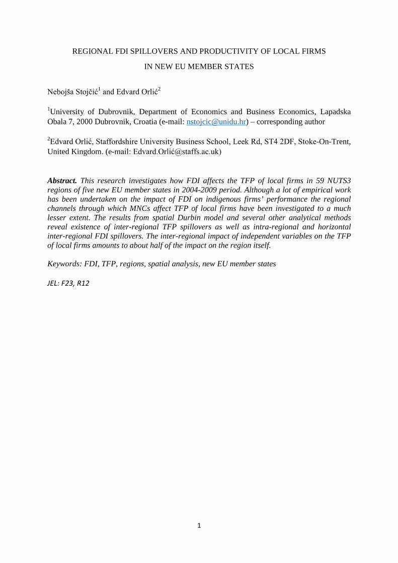
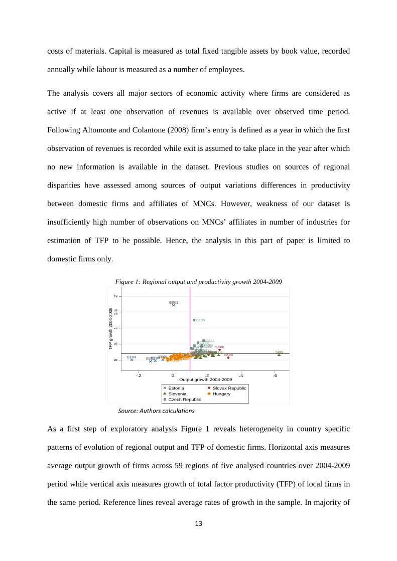
Figure 1: Regional output and productivity growth 2004-2009

Source: Authors calculations

As a first step of exploratory analysis Figure 1 reveals heterogeneity in country specific

patterns of evolution of regional output and TFP of domestic firms. Horizontal axis measures

average output growth of firms across 59 regions of five analysed countries over 2004-2009

period while vertical axis measures growth of total factor productivity (TFP) of local firms in

the same period. Reference lines reveal average rates of growth in the sample. In majority of

EE01

EE02EE03EE04 EE05

SK06SK01

SK08SK04SK07SK03

SK02SK05SI10SI11SI07SI03SI08SI12SI09SI02SI01 SI04

SI06SI05

HU18HU09HU19HU12HU01HU20HU03

HU06HU15

HU13HU16HU04

HU14HU02HU10HU17

HU11 HU07HU05

HU08

CZ03

CZ11

CZ05

CZ10CZ08

CZ07CZ14

CZ12

CZ09

CZ04

CZ01CZ02

CZ13

CZ06

0.5

11.

52

TFP

grow

th 2

004-

2009

-.2 0 .2 .4 .6Output growth 2004-2009

Estonia Slovak RepublicSlovenia HungaryCzech Republic

14

Estonian and Hungarian regions both growth of productivity of local firms as well as of

output was below sample average. In Slovenian regions the growth of output was above

sample average but the growth of GDP was below average. Finally, in majority of Slovak and

Czech regions both growth of output and of productivity were above sample average. In order

to shed further light on these findings, a previously defined method for decomposition of

output of domestic firms is applied (Table 1).

Table 1: The decomposition of changes in regional output in percentage terms (2004-2009) ΔYt Productivity Restructuring Covariance Net Entry

Czech Republic 1.08e+08 6.60 21.28 -26.46 -0.42 Estonia 5.42e+07 -0.12 0.15 -0.17 1.14 Hungary 1.65e+08 1.24 -0.58 -0.72 1.06 Slovak Republic 1.04e+07 1.11 1.22 -1.25 -0.08 Slovenia 9882708 0.96 0.01 -0.33 0.36 Source: Author’s calculations

Information in Table 1 refers to average output changes while table with detailed annual

decomposition can be found in Appendix. It enables the assessment of various channels

through which domestic firms contribute to the evolution of regional output. It appears that in

all countries except Estonia productivity changes positively contribute to the output. Another

channel of positive influence on regional output changes is restructuring suggesting that

increase in aggregate output is the result of reallocation of inputs to most productive firms

which is in line with Olley and Pakes (1996) and Foster et al (2001). The exception from this

finding is Hungary where reallocation of inputs contributes negatively to output change

suggesting that firms experiencing an increase in productivity are also loosing market shares

due to ongoing restructuring process.

Across all five countries a negative impact of covariance element can be observed. Altomonte

and Colantone (2008) interpret negative sign on this component as evidence of the ongoing

restructuring process where negative changes in variations of inputs have positive impact on

productivity. From there, the finding in our paper can be interpreted as further evidence of

rationalizing in use of inputs where firm experiencing an increase in productivity were losing

15

market shares due to restructuring and downsizing, rather than expansion (Bartelsman et al,

2004). The positive reallocation effects and negative covariance term may indicate divergence

in TFP, i.e. high productivity incumbent firms further increased their productivity and

allocative efficiency, while low productivity incumbents witnessed slow growth in TFP and

lost their market shares.

In the case of Slovenia, Hungary and Estonia a positive contribution of the net entry to the

dynamics of output is recorded. Such finding is in line with several earlier studies for new EU

member states that reported a positive contribution in terms of job creation and growth from

the net entry of new firms (De Loecker and Konings, 2005; Altomonte and Colantone, 2008).

This suggests the importance of creative destruction process where more productive firms

replace less productive ones. Hence, promoting policies which encourage competitive

behaviour should be important for productivity growth and regional output.

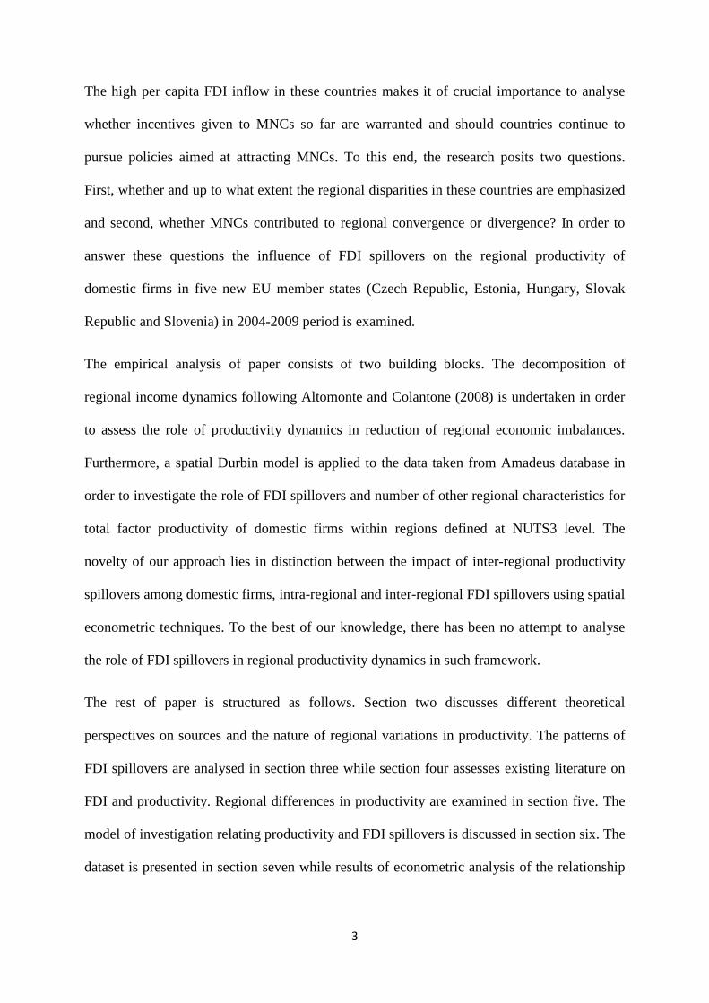
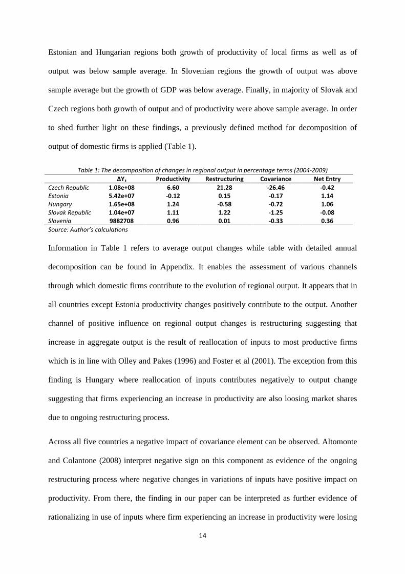
Figure 2: Moran I scatterplot of TFP growth rates over the 2004-2009 period

Source: Authors’ calculation

A question that arises in light of these findings is whether changes in productivity are spatially

correlated. As noted earlier, important channel for productivity improvements are spatial

technology and knowledge spillovers. The spatial autocorrelation can be defined as the

occurrence of value similarities in locational similarity (Anselin, 2001; Resmini and Nicolini,

2011). Spatial clustering of high or low values of variable in space is interpreted as positive

CZ03CZ11CZ05

CZ10

CZ08

CZ07

CZ14

CZ12

CZ09CZ04

CZ01

CZ02

CZ13

CZ06

SK06

SK01

SK08SK04SK07

SK03SK02SK05

HU18HU09HU19HU12

HU01

HU20HU03

HU06HU15

HU13HU16HU04HU14

HU02HU10

HU17

HU11

HU07HU05HU08SI10

SI11

SI07SI03SI08SI12

SI09SI02SI01

SI04

SI06

SI05

EE01

EE02

EE03

EE04EE05

-50

510

15w

TFP

gro

wth

(200

4-20

09)

-2 0 2 4 6TFP growth (2004-2009)

16

spatial autocorrelation while the opposite holds when high values of variable are surrounded

with low values (and vice versa).

In order to examine the existence of spatial autocorrelation a Moran scatterplot is used

(Anselin, 1996) where the spatial lag Wx of the variable x is plotted against variable itself. For

the purpose of this analysis, both levels and growth rates of TFP are plotted against their

spatial lags. Figure 2 plots TFP growth rates against their spatial lags indicating that growth

rates in our sample are spatially correlated.

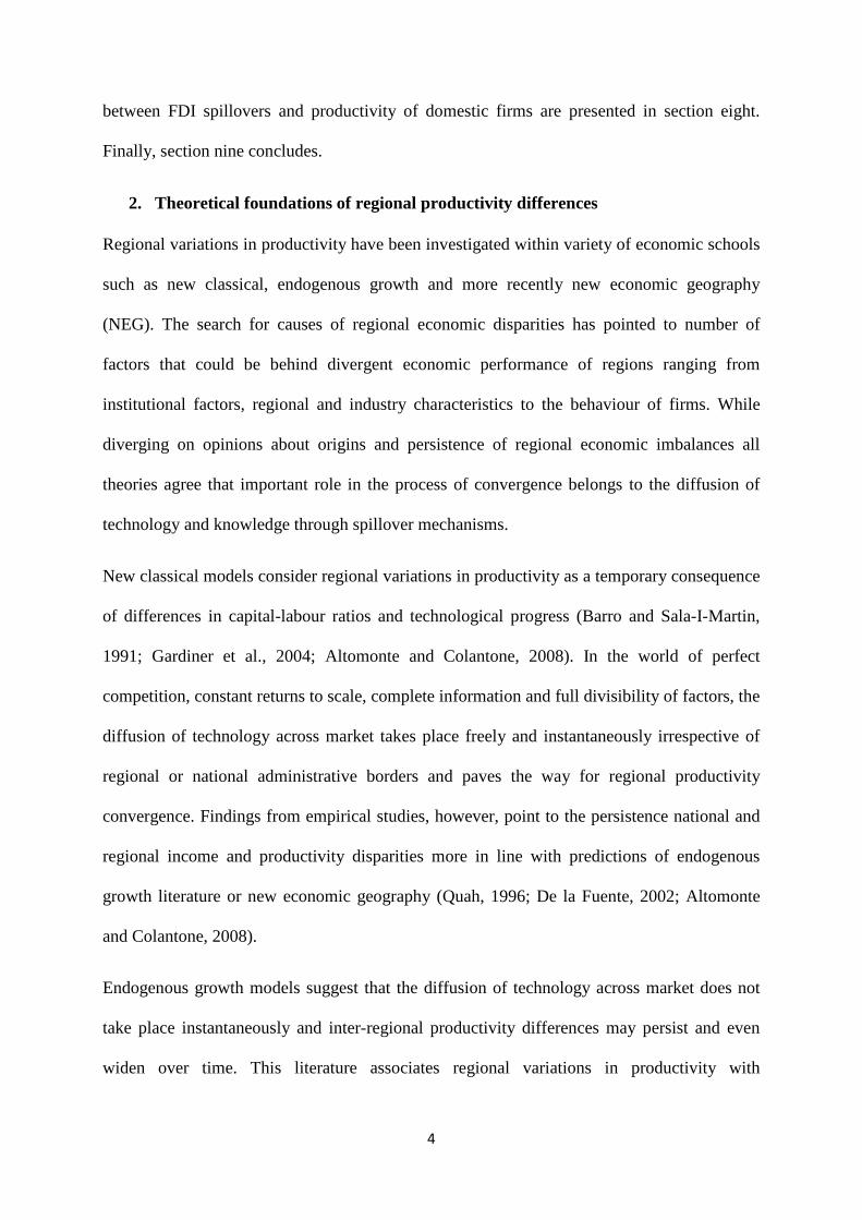
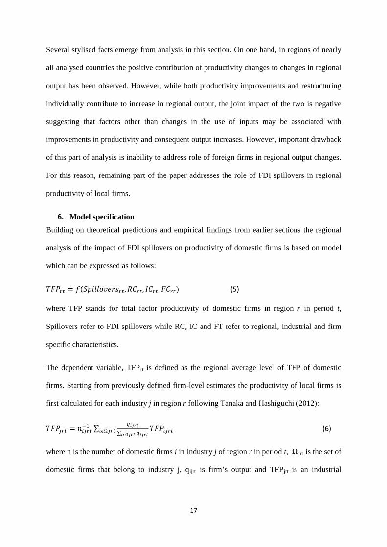
Figure 3: Moran I scatterplot of TFP levels (2004 and 2009)

Source: Authors’ calculations

Further evidence in favour of the thesis that our data follow systematic spatial pattern can be

found in Figure 3 which plots TFP levels in 2004 and 2009 against their spatial lags. In both

cases, similar to findings on growth rates (Figure 2), a positive pattern of spatial correlation

can be observed. For this reason, Moran’s test on spatial autocorrelation for both TFP growth

and levels is undertaken (Table 2). Under null hypothesis of this test there is zero spatial

autocorrelation. The results in Table 2 reveal existence of positive spatial autocorrelation and

consistent with findings from earlier literature on new EU member states suggest that the

spatial correlation is stronger in levels than in growth form (Resmini and Nicolini, 2011).

Table 2: Moran’s two-tail test for spatial autocorrelation of TFP levels and growth Variable I E(I) sd(I) Z p-value TFP growth 0.016 -0.017 0.022 1.514 0.065 2004 level 0.014 -0.017 0.018 1.696 0.045 2009 level 0.040 -0.017 0.022 2.576 0.010

Source: Authors’ calculations

CZ03CZ11CZ05CZ10CZ08CZ07

CZ14CZ12CZ09CZ04

CZ01CZ02

CZ13

CZ06EE01

EE02

EE03EE04EE05

HU18

HU09

HU19

HU12

HU01

HU20

HU03

HU06

HU15

HU13

HU16

HU04

HU14HU02

HU10

HU17

HU11HU07

HU05

HU08

SI10SI11SI07SI03SI08SI12SI09

SI02SI01

SI04SI06SI05

SK06

SK01

SK08

SK04

SK07

SK03SK02

SK05

-.20

.2.4

Spat

ial l

ag T

FP le

vel i

n 20

04

0 2 4 6TFP level in 2004

CZ03CZ11

CZ05CZ10CZ08CZ07

CZ14CZ12CZ09CZ04

CZ01CZ02

CZ13

CZ06SI10SI11SI07SI03SI08SI12SI09

SI02SI01

SI04SI06SI05

SK06

SK01

SK08

SK04SK07

SK03SK02

SK05

HU18HU09

HU19

HU12

HU01

HU20

HU03

HU06

HU15 HU13

HU16

HU04

HU14

HU02

HU10

HU17

HU11

HU07

HU05

HU08

EE01EE02EE03EE04EE05

-.20

.2.4

.6.8

Spa

tial l

ag T

FP le

vel i

n 20

09

0 1 2 3 4 5TFP level in 2009

17

Several stylised facts emerge from analysis in this section. On one hand, in regions of nearly

all analysed countries the positive contribution of productivity changes to changes in regional

output has been observed. However, while both productivity improvements and restructuring

individually contribute to increase in regional output, the joint impact of the two is negative

suggesting that factors other than changes in the use of inputs may be associated with

improvements in productivity and consequent output increases. However, important drawback

of this part of analysis is inability to address role of foreign firms in regional output changes.

For this reason, remaining part of the paper addresses the role of FDI spillovers in regional

productivity of local firms.

6. Model specification

Building on theoretical predictions and empirical findings from earlier sections the regional

analysis of the impact of FDI spillovers on productivity of domestic firms is based on model

which can be expressed as follows:

𝑇𝐹𝑃𝑟𝑡 = 𝑓(𝑆𝑝𝑖𝑙𝑙𝑜𝑣𝑒𝑟𝑠𝑟𝑡,𝑅𝐶𝑟𝑡, 𝐼𝐶𝑟𝑡,𝐹𝐶𝑟𝑡) (5)

where TFP stands for total factor productivity of domestic firms in region r in period t,

Spillovers refer to FDI spillovers while RC, IC and FT refer to regional, industrial and firm

specific characteristics.

The dependent variable, TFPrt is defined as the regional average level of TFP of domestic

firms. Starting from previously defined firm-level estimates the productivity of local firms is

first calculated for each industry j in region r following Tanaka and Hashiguchi (2012):

𝑇𝐹𝑃𝑗𝑟𝑡 = 𝑛𝑖𝑗𝑟𝑡−1 ∑ 𝑞𝑖𝑗𝑟𝑡∑ 𝑞𝑖𝑗𝑟𝑡𝑖𝜖Ω𝑗𝑟𝑡

𝑖𝜖Ω𝑗𝑟𝑡 𝑇𝐹𝑃𝑖𝑗𝑟𝑡 (6)

where n is the number of domestic firms i in industry j of region r in period t, Ωjrt is the set of

domestic firms that belong to industry j, qijrt is firm’s output and TFPjrt is an industrial

18

average of firm productivity in a given industry and region. From there, the regional average

of firm productivity can be calculated as:

𝑇𝐹𝑃𝑟𝑡 = 𝑚𝑟𝑡−1 ∑ 𝑇𝐹𝑃𝑗𝑟𝑡𝑗𝜖𝑟𝑡 (7)

where m is the number of industries in given region. Hence, in construction of regional

average of firm productivity TFP of each firm is weighted by its output share in industry.

Several authors have warned that input shares of each firm might be better weights as output

is dependent on productivity (Foster et al., 2001; Altomonte and Colantone, 2008). In order to

check for robustness of results alternative measure of TFP is also constructed using input

shares as weights.

The modelling of spillovers begins with standard approach in the literature (Javorcik, 2004),

and makes distinction between horizontal, vertical backward and vertical forward spillovers.

The regional average of intra-industry or horizontal spillovers is calculated as follows:

𝐻𝑜𝑟𝑖𝑧𝑜𝑛𝑡𝑎𝑙𝑟𝑡 = 𝑚𝑟𝑡−1 ∑ 𝑞𝑗𝑟𝑡

∑ 𝑞𝑗𝑟𝑡𝑗𝜖Ω𝑟𝑡∗∑ 𝐹𝑜𝑟𝑒𝑖𝑔𝑛𝑖𝑗𝑟𝑡∗𝑞𝑖𝑗𝑟𝑡𝑖𝜖Ω𝑗𝑟𝑡

∑ 𝑞𝑖𝑗𝑟𝑡𝑖𝜖Ω𝑗𝑟𝑡𝑗𝜖Ω𝑟𝑡 (8)

where qijrt is the output produced by firm i in industry j and region r in year t , m is number of

industries in region r and Foreignit is a dummy variable indicating foreign participation in

firm i in year t2 while qjrt is the output of industry j in region r and year t. Hence, in order to

capture regional differences in industry composition, spillovers for each industry are weighted

with share of given industry in regional output prior to calculation of regional average.

The computation of technical coefficients for vertical linkages departs from standard approach

in the literature and includes inputs supplied within the same industry. The reason for this lies

in the fact that it is unrealistic to assume no intra-industry linkages in highly aggregated

2 Firm is considered foreign if the sum of shares of foreign investors exceeds 10% of its equity. Ownership information is available for each year and for each firm. In the calculation of horizontal measure the total number of firms available in the database was used regardless whether these firms had data on all production variables for TFP estimation.

19

industries. Therefore, exclusion of inputs supplied within the same industry might affect

empirical results (Leanerts and Merlevede, 2013). The backward vertical linkages can be

calculated as follows:

𝐵𝑎𝑐𝑘𝑤𝑎𝑟𝑑𝑟𝑡 = 𝑚𝑟𝑡−1 ∑ 𝑞𝑗𝑟𝑡

∑ 𝑞𝑗𝑟𝑡𝑗𝜖Ω𝑟𝑡∗ ∑ 𝛼𝑗𝑘𝑟𝑡𝐻𝑜𝑟𝑖𝑧𝑜𝑛𝑡𝑎𝑙𝑘𝑟𝑡𝑘

𝑗=1𝑗𝜖Ω𝑟𝑡 (9)

where industrial horizontal spillovers are multiplied with the technical coefficient from input-

output tables and previously defined industry weights. In this case, technical coefficient 𝛼𝑗𝑘𝑟𝑡

is the proportion of industry j’s output supplied to industry k in period t. Hence, the backward

linkage captures spillovers between MNCs and local suppliers. The technical coefficients

𝛼𝑗𝑘𝑟𝑡are calculated for domestic intermediate consumption excluding final uses, export and

imports. This way, the common assumption that MNCs employ domestic inputs in the same

proportion as imported inputs is relaxed. While both types of inputs can increase TFP of

domestic firms, MNCs may source different inputs in host country (Barrios et al., 2011).

Analogously, forward linkages can be calculated as:

𝐹𝑜𝑟𝑤𝑎𝑟𝑑𝑟𝑡 = 𝑚𝑟𝑡−1 ∑ 𝑞𝑗𝑟𝑡

∑ 𝑞𝑗𝑟𝑡𝑗𝜖Ω𝑟𝑡∗ ∑ 𝛾𝑘𝑗𝑟𝑡𝐻𝑜𝑟𝑖𝑧𝑜𝑛𝑡𝑎𝑙𝑘𝑟𝑡𝑘

𝑗=1𝑗𝜖Ω𝑟𝑡 (10)

In this case technical coefficient 𝛾𝑘𝑗𝑡 the proportion of industry j’s inputs purchased from

industries k at time t. The forward linkage is a proxy for spillovers between MNCs and their

local clients. The larger the presence of MNCs in upstream sectors k and the larger the output

sold to local firms the higher is the value of the variable.

Model of investigation also includes several control variables. Regional characteristics

include measures of net migration share, human capital and agglomeration economies. The

net migration share in total population is defined as the absolute share of the difference

between count of new residents in the region and the residents leaving region divided by total

regional population. Migration is associated with the brain circulation” paradigm according to

20

which immigrants create benefits for destination countries and regions in terms of creativity

and innovations (Saxenian, 1999; Florida, 2002). Hence, it is expected that higher migration

has beneficial effect on TFP of local firms. Regional human capital is proxied with the share

of workers employed in high technology intensive industries and it is expected to have

positive sign. Finally, two variables are included reflecting agglomeration economies, defined

as urbanisation and localisation economies. As noted in section 2 of paper, NEG literature

points to the beneficial impact of geographical proximity of firms with their counterparts,

professional and scientific institutions (Krugman, 1991; Venables, 1996; Hafner, 2013).

The urbanisation economies aim to capture between-industry spillovers from inter-sectoral

diversity such as sharing of basic assets, information, resources and institutions while

localisation economies control for within industry factors such as learning, contact with early

adapters or information about market conditions (Stojcic et al., 2013). The urbanisation

economies is measured as the ratio between the number of all firms in region and the total

number of firms in country while regional average of localisation economies is measured as

the regional average of a ratio between the number of firms belonging to same industry and

all firms within a given region. A positive sign could be expected for these variables.

Among industry specific characteristics the regional average of industrial concentration is

included. The measure of horizontal spillovers may also capture competition effects for which

reason it is necessary to isolate these two effects. Foreign entry may increase the intensity of

competition thus forcing local firms to become more efficient and productive. The failure to

control for the intensity of competition could attribute increases in TFP of local firms to

spillovers. For this reason, Herfindahl-Hirschman concentration index is employed as a

measure of competition intensity. The sign of this variable is expected to be negative.

We also include average firm size in region. On the one hand, firm size, measured as number

of employees, is expected to control for absorption of spillovers and productivity enhancing

21

processes. As noted by Farole and Winkler (2012) larger firms usually have large number of

trained and skilled people, more competent management, pay higher wages and are also more

visible, thus are more likely to be selected as suppliers and become clients of MNCs. Yet,

smaller firms may be more responsive to changing business environment. Therefore for this

variable there are no expectations regarding its sign. Finally, several variables are included

measuring the quality of institutional environment on national level. These include business

freedom, intellectual property rights quality and investment freedom. The latter factors are

important for both domestic and foreign firms as reliable institutional environment reduces

the risk and uncertainties related to imperfect information (North, 1990), creates incentives

and business practices that facilitate knowledge acquisition process (Meyer and Sinani, 2009)

and act as a determinant of both quantity and quality of FDI which may influence the

potential and magnitude of spillovers.

7. Data and methodology

As noted previously, primary source of data in this analysis is the firm-level database

Amadeus produced by Bureau van Dyke. The data from this database have been used to

construct variables of regional TFP of local firms, FDI spillovers, concentration index,

urbanisation and localisation economies, average regional firm size and the proportion of

workers in high-tech industries. In order to estimate previously defined model this database

has been combined with several other sources.

The calculation of vertical FDI spillovers would not have been possible without the use of

input-output tables. These were taken from World Input Output Database used previously by

Timmer (2012). Being published only recently, this database provides yearly input output

tables aggregated over 35 sectors at 2-digit level. The advantage of annual data is possibility

of estimation of time varying input output coefficients which is a significant improvement

over previous studies which used IO tables from early/mid 2000s, thus reflecting the changing

22

economic structure of countries over years. The data on migration are taken from OECD

regional statistics database. Finally, in order to measure the quality of institutional

environment the data on business freedom, investment freedom and IPR are taken from

Heritage Foundation. As previously, data in this part of analysis cover period between 2004

and 2009 in 59 NUTS3 regions of five new EU member states.

Findings from section 5 and longitudinal nature of our dataset suggest that suitable estimator

should be looked for within family of spatial panel estimators. Broadly speaking, spatial

dependence among observations can be investigated with four main types of estimators

known as spatial autoregression model (SAR), spatial error model (SEM), Durbin spatial

autoregression model (DSAR) and general spatial error model (GSAR). In simplest form SAR

model can be defined as:

𝑦𝑖𝑡 = 𝜌∑ 𝑤𝑖𝑗𝑦𝑗𝑡 + 𝛽𝑋𝑖𝑡 +𝑛𝑗=1 𝜀𝑖𝑡 (11)

Equation (11) establishes a direct relationship between the dependent variable yit for cross

sectional unit i in period t and the dependent variables yjt of other cross-sectional units. The

expression ∑ 𝑤𝑖𝑗𝑦𝑗𝑡𝑛𝑗=1 is the interaction effect of the dependent variable yit with the

dependent variables of other units (yjt) while wij is the i,j-th element of a prespecified

nonnegative NxN spatial weights matrix W and (𝜌) is spatial dependence parameter. Finally,

X and β stand for the regional independent variables and their respective coefficients while 𝜀

is idiosyncratic error term. This specification reveals whether the TFP of local firms in given

region and time period is affected with TFP of local firms in other regions.

The spatial error model (SEM) imposes specific structure to the unobserved factors

influencing dependent variable which would otherwise be captured by the error term

(Blonigen et al., 2007; Kayam et al., 2013). The model is specified as follows:

𝑦𝑖𝑡 = 𝛽𝑋𝑖𝑡 + 𝜀𝑖𝑡, 𝜀𝑖𝑡 = 𝜌∑ 𝑤𝑖𝑗𝜀𝑗𝑡𝑛𝑗=1 + 𝑢𝑖𝑡 (12)

23

where 𝜌 is the spatial autocorrelation coefficient. The use of SEM model allows to investigate

the impact of shocks in dependent variable of other cross-sectional units (regions) to the

dependent variable of region i.

DSAR and GSEM models can be considered as extensions of the two previously discussed

(Le Sage and Pace, 2009; Elhorst, 2013). Durbin spatial autoregression model (DSAR) can be

defined as:

𝑦𝑖𝑡 = 𝜌∑ 𝑤𝑖𝑗𝑦𝑗𝑡 + 𝛽𝑋𝑖𝑡 +𝑛𝑗=1 𝜃 ∑ 𝑤𝑖𝑗𝑥𝑗𝑡𝑛

𝑗=1 + 𝜀𝑖𝑡 (13)

In equation (13) the dependent variable of particular unit depends on independent explanatory

variables of the dependent variables of other units. One can observe how FDI spillovers to

other regions influence the TFP of local firms in a given region. Finally, the general spatial

error model (GSEM) adds the spatially weighted dependent variables matrix to the right hand

side of the error term (Baltagi et al., 2007). It takes form of:

𝑦𝑖𝑡 = 𝛽1𝑋𝑖𝑡 + 𝛽2𝑤𝑖𝑗𝑋𝑗𝑡 + 𝜀𝑖𝑡, 𝜀𝑖𝑡 = 𝜌∑ 𝑤𝑖𝑗𝜀𝑗𝑡𝑛𝑗=1 + 𝑢𝑖𝑡 (14)

The selection of appropriate spatial estimator involves choice between conventional and

spatial econometric techniques on the basis of Lagrange Multiplier (LM) tests for a spatially

lagged dependent variable and for spatial error autocorrelation as well as the testing for the

existence of one type of spatial dependence conditional on the other using robust LM,

Likelihood Ratio (LR) or Wald tests (Elhorst, 2013). Burridge (1981) notes that spatial

Durbin model should be given preference when hypotheses of H0: 𝜃=0 and H0: 𝜃 + 𝜌𝛽=0 are

both rejected. Conversely if one of these hypotheses cannot be rejected spatial lag or spatial

error models should be used.

Findings from spatial dependence analyses are sensitive on the specification of the weighting

matrix (W), a symmetric NxN matrix, where N is the number of units that defines position of

cross-sectional units in space with respect to each other (Anselin, 1999; Le Sage, 1998; 1999).

24

In order to examine robustness of our results, two alternative specifications of W are

employed, “neighbourhood” matrix where wij takes value of 1 if regions i and j are

neighbours and 0 otherwise and another one where the wij is defined as inverse distance

between regional centres (Baltagi et al., 2007). Furthermore, following standard procedure

each weight matrix is row standardized with elements wij of each row having sum of 1

(Olejnik, 2008).

Findings from spatial regressions are usually interpreted on the basis of point estimates. Le

Sage and Pace (2009) suggest that a partial derivative interpretation of the impact from

changes to the variables of different model specifications is a far better approach. Following

this approach a distinction can be made between the effect of a change of a particular

explanatory variable in a particular spatial unit on the dependent variable of all other units in

the short run and in the long run. Furthermore, it has been suggested by several authors that

spatial non-stationarity may lead to spurious regression (Fingleton, 1999; Olejnik, 2008;

Elhorst, 2013). As noted by Le Sage and Pace (2009) for this reason the condition 𝜌 ∈

(1 𝑟𝑚𝑖𝑛⁄ , 1) is imposed where rmin equals the most negative purely real characteristic root of

W after this matrix has been row-normalized. In that case, the dependent variable can be said

to follow spatially integrated process of SI(0).

Two prevalent methods of estimation have been applied to the above models, maximum

likelihood method (ML) and generalised method of moments (GMM). Some authors note that

GMM estimator can be severely biased due to endogeneity in spatially lagged dependent

variable WYt (Elhorst, 2010; Lee and Yu, 2014). Bearing everything above said in mind the

model is estimated using maximum likelihood estimator and standard procedure for selection

of appropriate model is applied. Furthermore, in addition to point estimates the analysis also

makes distinction between indirect and direct effect of spillovers. Finally, robust standard

errors are employed in order to control for potential heteroscedasticity.

25

8. Discussion of findings

Building on theoretical arguments and research methodology discussed above the model in

following form is being estimated:

𝑙𝑛𝑇𝐹𝑃𝑖𝑡 = 𝑐0 + 𝜌∑ 𝑤𝑖𝑗𝑙𝑛𝑇𝐹𝑃𝑗𝑡𝑛𝑗=1 + 𝛽1ℎ𝑜𝑟𝑖𝑧𝑜𝑛𝑡𝑎𝑙𝑖𝑡 + 𝛽2𝑓𝑜𝑟𝑤𝑎𝑟𝑑𝑖𝑡 + 𝛽3𝑏𝑎𝑐𝑘𝑤𝑎𝑟𝑑𝑖𝑡 +

𝜃1 ∑ 𝑤𝑖𝑗ℎ𝑜𝑟𝑖𝑧𝑜𝑛𝑡𝑎𝑙𝑗𝑡𝑛𝑗=1 + 𝜃2 ∑ 𝑤𝑖𝑗𝑓𝑜𝑟𝑤𝑎𝑟𝑑𝑗𝑡𝑛

𝑗=1 + 𝜃3 ∑ 𝑤𝑖𝑗𝑏𝑎𝑐𝑘𝑤𝑎𝑟𝑑𝑗𝑡𝑛𝑗=1 + 𝛽4𝑙𝑛𝑚𝑖𝑔𝑟𝑎𝑡𝑖𝑜𝑛 𝑖𝑡 +

𝛽5𝑙𝑛𝑐𝑜𝑛𝑐𝑒𝑛𝑡𝑟𝑎𝑡𝑖𝑜𝑛𝑖𝑡 + 𝛽6𝑙𝑛𝑢𝑟𝑏𝑎𝑛𝑖𝑠𝑎𝑡𝑖𝑜𝑛𝑖𝑡 + 𝛽7𝑙𝑛𝑙𝑜𝑐𝑎𝑙𝑖𝑠𝑎𝑡𝑖𝑜𝑛𝑖𝑡 + 𝛽8ℎ𝑐𝑎𝑝𝑖𝑡𝑎𝑙𝑖𝑡 +

𝛽9𝑙𝑛𝑒𝑚𝑝𝑙𝑜𝑦𝑒𝑒𝑠𝑖𝑡 + 𝛽10𝑙𝑛𝑏𝑢𝑠𝑠𝑐𝑡 + 𝛽11𝑙𝑛𝑖𝑛𝑣𝑐𝑡 + 𝛽12𝑙𝑛𝑖𝑝𝑟𝑐𝑡 + 𝜆∑ 𝜀𝑗𝑡𝑛𝑗=1 + 𝑢𝑖𝑡

(15)

Equation 15 is known as the spatial Durbin model discussed in previous section. The model is

specified in semi-logarithmic form with all variables taking positive values entering model in

logarithm form while variables containing zeros and negative values enter model in levels

form. It is estimated with maximum likelihood method robust to presence of non-normality

and heteroscedasticity. As our main interest lies in the relationship between productivity of

local firms and FDI spillovers the analysis of spatial effects is limited to these variables.

However, prior to discussion of results the procedure for model selection and relevant model

diagnostics are addressed.

8.1. Model diagnostics

Relevant model diagnostics are presented in Table 3. In models (1) and (2) inverse distance

spatial weight matrix is used while neighbourhood matrix is used in models (3) and (4).

Furthermore, the dependent variable of models (1) and (3) has input shares as weights while

output shares are used in models (2) and (4). In all four models the null hypothesis of Wald

test that variables jointly have no explanatory power is rejected with very high probability.

The value of coefficient 𝜌 falls within its acceptable range which suggests that the dependent

variable follows spatially integrated process SI(0) (Le Sage and Pace, 2009). Finally, LR tests

in Table 3 demonstrate that null hypotheses of spatially lagged dependent variable and spatial

26

lags of regressors being equal to zero are rejected with very high probability in all four

models. This suggests that spatial estimation techniques should be preferred over

conventional econometric analysis (Elhorts, 2013; Shehata and Mickaiel, 2014).

Table 3: Model diagnostics

Model (1) (2) (3) (4) Number of observations 354 354 354 354 Number of units (regions) 59 59 59 59 Log likelihood function -770.57 -773.62 -772.19 -776.08 Wald test 259.6*** 269.8*** 331.30*** 354.46*** LR TEST SDM vs. OLS 𝐻0: (𝜌 = 0) 31.26*** 36.41*** 9.38*** 10.89*** LR TEST 𝐻0: (𝑤𝑋′𝑠 = 0) 11.83*** 11.62*** 19.72*** 19.22*** 𝜌 0.61 0.63 0.21 0.22 Acceptable range for 𝜌 -2.8< 𝜌<1 -2.8< 𝜌<1 -1.6< 𝜌<1 -1.6< 𝜌<1 Spatial Error Autocorrelation Tests H0: (no spatial error autocorrelation)

Global Moran MI 0.19*** 0.22*** 0.11*** 0.13*** Global Geary GC 0.82*** 0.80*** 0.88*** 0.86*** Global Getis-Ords GO -0.19*** -0.22**** -0.11*** 0.13*** Moran MI Error Test 17.19*** 19.06*** 3.44*** 3.84*** LM Error (Burridge) 115.26*** 143.50*** 5.27** 6.79** LM Error (Robust) 106.77** 136.31*** 0.02 0.01 Spatial Lagged Dependent Variable Tests H0: (no spatial autocorrelation)

LM Lag (Anselin) 46.69*** 56.34*** 6.67** 8.55** Lm Lag (Robust) 38.20*** 49.15*** 1.41 1.77 General Spatial Autocorrelation Tests H0: (no general spatial autocorrelation)

LM SAC (LMErr+LMLag_R) 153.47*** 192.65*** 6.69** 8.56** LM SAC (LMLag+LMErr_R) 153.47*** 192.65*** 6.69** 8.56**

Note: ***,** and * denote statistical significance at 1%, 5% and 10% level of significance respectively

Further testing procedure involves conventional and robust LM tests in order to determine the

proper spatial estimator (Burridge, 1980; Anselin, 1988). Common procedure suggests that

spatial lag model should be given preference if its LM test is more significant than LM test for

spatial error and robust LM test for spatial error is not significant while in opposite case

spatial error model should be preffered (Shehata and Mickaiel, 2014). Also, when LM tests

for both spatial lag and spatial error are significant or the conventional LR tests and robust

LM tests point to different models preference should be given to spatial Durbin model

(Elhorst, 2011). Following above described procedure it is evident that in all four

specifications model diagnostics suggest that spatial Durbin model should be preferred over

other spatial estimators. Overall, these diagnostics indicate robustness of selected models and

allow us to proceed with interpretation of results.

27

8.2. Interpretation of results

Results of estimation are presented in Table 3 where as previously models (1) and (2) are

estimated using inverse distance spatial weight matrix while neighbourhood matrix is used in

models (3) and (4). The dependent variable of models (1) and (3) has input shares as weights

while output shares are used in models (2) and (4). First striking finding is robustness of

results with respect to sign and significance across all four specifications. Moreover, with

exception of spatially lagged dependent variable all coefficients are of similar magnitude

providing further support to the robustness of our model. Across all four models, a positive

spatial spillovers of TFP among local firms can be observed. The magnitude of coefficient

ranges from 0.22 in models with neighbourhood matrix to the 0.63 in models with inverse

distance matrix. These findings are in line with evidence from earlier literature suggesting

increase of coefficient on spatially lagged dependent variable when full inverse distance

matrix is used (e.g. Seldadyo et al., 2010).

Table 4: Results of estimation Model (1) (2) (3) (4) Variable Spatial lag of dependent variable ln (wTFP) 0.61*** 0.63*** 0.21*** 0.22*** FDI SPILLOVERS Backward FDI spillovers (backward) -0.003* -0.003* -0.003* -0.003* Forward FDI spillovers (forward) 0.01** 0.01* 0.01** 0.01** Horizontal FDI spillovers (horizontal) -0.17*** -0.17*** -0.18*** -0.18*** Backward FDI spillovers – spatial lag (wbackward) 0.003 0.003 -0.003 -0.002 Forward FDI spillovers – spatial lag (wforward) 0.02 0.02 0.01 0.01 Horizontal FDI spillovers – spatial lag (whorizontal) -0.76*** -0.76*** -0.40*** -0.40*** REGIONAL CHARACTERISTICS Net migration share in population ln(migration) 0.15 0.130 0.21* 0.19* Average industry concentration ln (hhi) -1.18*** -1.27*** -1.08*** -1.17*** Urbanisation externalities ln (urbanisation) 0.79 *** 0.82*** 0.87*** 0.90*** Localisation externalities ln (localisation) -0.37 -0.34 -0.60 -0.57 Human capital (hcapital) 0.34 0.28 0.57 0.51 Average firm size ln (emp) 0.95*** 0.96*** 0.91*** 0.92*** INSTITUTIONAL ENVIRONMENT Business freedom ln (buss) 2.34 2.48 2.27 2.40 Investment freedom ln (inv) -0.19 -0.17 0.46 0.56 Protection of intellectual property rights ln (ipr) 2.43*** 2.43*** 2.92*** 2.94*** Constant term (cons) -17.65 -18.61* -18.30 -19.41

Source: Authors’ calculations Note: p-values in brackets where ***,** and * denote statistical significance at 1%, 5% and 10% level of significance respectively

28

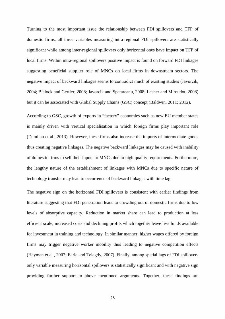
Turning to the most important issue the relationship between FDI spillovers and TFP of

domestic firms, all three variables measuring intra-regional FDI spillovers are statistically

significant while among inter-regional spillovers only horizontal ones have impact on TFP of

local firms. Within intra-regional spillovers positive impact is found on forward FDI linkages

suggesting beneficial supplier role of MNCs on local firms in downstream sectors. The

negative impact of backward linkages seems to contradict much of existing studies (Javorcik,

2004; Blalock and Gertler, 2008; Javorcik and Spatareanu, 2008; Lesher and Miroudot, 2008)

but it can be associated with Global Supply Chains (GSC) concept (Baldwin, 2011; 2012).

According to GSC, growth of exports in “factory” economies such as new EU member states

is mainly driven with vertical specialisation in which foreign firms play important role

(Damijan et al., 2013). However, these firms also increase the imports of intermediate goods

thus creating negative linkages. The negative backward linkages may be caused with inability

of domestic firms to sell their inputs to MNCs due to high quality requirements. Furthermore,

the lengthy nature of the establishment of linkages with MNCs due to specific nature of

technology transfer may lead to occurrence of backward linkages with time lag.

The negative sign on the horizontal FDI spillovers is consistent with earlier findings from

literature suggesting that FDI penetration leads to crowding out of domestic firms due to low

levels of absorptive capacity. Reduction in market share can lead to production at less

efficient scale, increased costs and declining profits which together leave less funds available

for investment in training and technology. In similar manner, higher wages offered by foreign

firms may trigger negative worker mobility thus leading to negative competition effects

(Heyman et al., 2007; Earle and Telegdy, 2007). Finally, among spatial lags of FDI spillovers

only variable measuring horizontal spillovers is statistically significant and with negative sign

providing further support to above mentioned arguments. Together, these findings are

29

consistent with evidence reviewed in section 4 on the existence of intra-regional FDI

spillovers and no or negative inter-regional impact on TFP of local firms.

The negative sign on industrial concentration suggests that the concentration of market share

among smaller number of firms likely comes at the expense of domestic firms which leaves

them with less funds for investment in improvements in efficiency. Positive impact of

urbanisation economies further supports such reasoning. Moreover, large firms seem to be

more productive which as noted earlier can be associated with higher pool of trained and

skilled employees, better management and visibility to MNCs (Farole and Winkler, 2012).

The positive impact of net migration is also observed in models (3) and (4) suggesting that

transfer of ideas and creativity contribute positively to TFP of local firms. Finally, among

institutional variables protection of intellectual property rights is significant with positive

sign. This finding may signal that the ability of firms to protect their intellectual property acts

as incentive to innovate which in turn has beneficial effect on their total factor productivity.

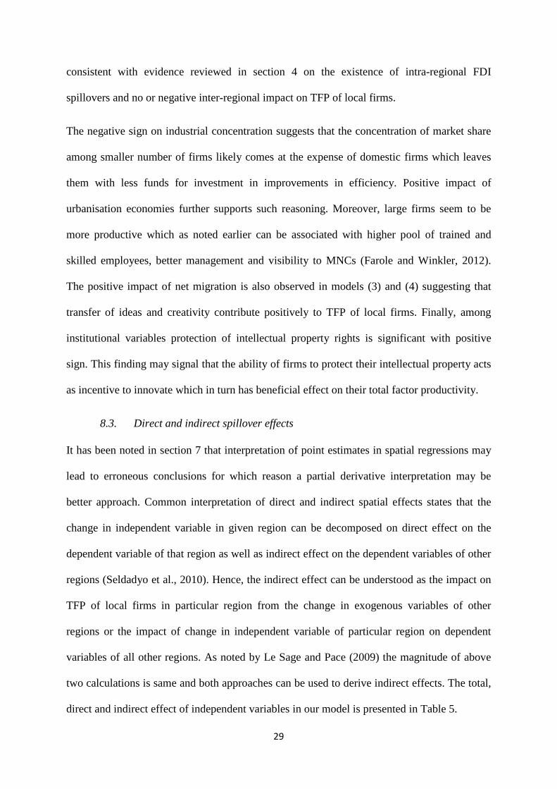
8.3. Direct and indirect spillover effects

It has been noted in section 7 that interpretation of point estimates in spatial regressions may

lead to erroneous conclusions for which reason a partial derivative interpretation may be

better approach. Common interpretation of direct and indirect spatial effects states that the

change in independent variable in given region can be decomposed on direct effect on the

dependent variable of that region as well as indirect effect on the dependent variables of other

regions (Seldadyo et al., 2010). Hence, the indirect effect can be understood as the impact on

TFP of local firms in particular region from the change in exogenous variables of other

regions or the impact of change in independent variable of particular region on dependent

variables of all other regions. As noted by Le Sage and Pace (2009) the magnitude of above

two calculations is same and both approaches can be used to derive indirect effects. The total,

direct and indirect effect of independent variables in our model is presented in Table 5.

30

Table 5:Direct and indirect marginal effects Model (1) (2) (3) 4 Variable Direct

effect Indirect effect

Direct effect

Indirect effect

Direct effect

Indirect effect

Direct effect

Indirect effect

FDI SPILLOVERS Backward -0.001 -0.002 -0.001 -0.002 -0.003 -0.001 -0.002 -0.001 Forward 0.003 0.004 0.002 0.004 0.006 0.002 0.005 0.002 Horizontal -0.065 -0.098 -0.062 -0.103 -0.139 -0.035 -0.139 -0.037 Wbackward 0.001 0.002 0.001 0.002 -0.002 -0.001 -0.002 -0.0004 Wforward 0.008 0.012 0.008 0.013 0.007 0.002 0.006 0.002 Whorizontal -0.296 -0.449 -0.279 -0.459 -0.319 -0.080 -0.311 -0.084 REGIONAL CHARACTERISTICS ln(migration) 0.057 0.086 0.048 0.079 0.165 0.041 0.149 0.040 ln (hhi) -0.458 -0.696 -0.468 -0.770 -0.858 -0.214 -0.909 -0.245 ln (urbanisation) 0.306 0.465 0.300 0.494 0.686 0.171 0.697 0.188 ln (localisation) -0.144 -0.218 -0.124 -0.204 -0.473 -0.118 -0.447 -0.120 (hcapital) 0.133 0.203 0.104 0.171 0.448 0.112 0.396 0.107 ln (emp) 0.368 0.558 0.354 0.583 0.722 0.180 0.718 0.194 INSTITUTIONAL ENVIRONMENT ln (buss) 0.905 1.374 0.911 1.501 1.799 0.449 1.865 0.503 ln (inv) -0.075 -0.114 -0.061 -0.101 0.367 0.092 0.432 0.117 ln (ipr) 0.941 1.429 0.894 1.472 2.310 0.576 2.286 0.616

Source: Author’s calculations

Findings from Table 5 reveal two interesting features. First, it is evident that the direct effects

are different from the estimates of parameters which can be explained with feedback effect.

Seldadyo et al. (2010) note that the impact of particular explanatory variables is partly

realised through neighbouring regions and back to original region. Second, while there

appears to be no sensitivity on the construction of dependent variable, results are sensitive on

the specification of spatial weight matrix. The direct effects are almost twice as large when

first-neighbour matrix is used than with full inverse distance matrix while opposite holds for

indirect effects.

Bearing in mind findings from previous section about the sensitivity of spatially lagged

dependent variable coefficient magnitude on the choice of matrix W together with findings of

this section, a logical question arises which of above specifications best describes analysed

data. Some of earlier studies advocate comparison of log-likelihood function values where the

model with highest values should be preferred (Seldadyo et al., 2010). Model diagnostics in

Table 3 suggest that specification (4) using nearest neighbour matrix and output shares as TFP

weights has highest log-likelihood value. In view of these findings one can conclude that the

31

TFP of local firms in one region is related to TFP of local firms in surrounding regions with

the magnitude of impact of about 0.22%. Furthermore, there is evidence of intra-regional and

horizontal inter-regional FDI spillover impact on TFP of local firms. Finally, the impact of

change in independent variable of individual regions on the TFP of local firms in other

regions amounts to about 50% of the impact on the region itself.

9. Conclusion

Over past decades significant efforts have been invested by policy makers in new EU member

states to attract FDI. The underlying reasoning behind these activities has been theoretical

prediction and empirical evidence about the beneficial impact of FDI on host economy,

particularly on the ability of its firms to compete on both domestic and international markets

through horizontal, backward and forward spillovers. Nevertheless recent figures point that

majority of regions in CEECs are still lagging behind EU27 average in terms of GDP per

capita. Bearing in mind high inflow of FDI in these countries over past decades the objective

of this research was to investigate whether incentives given to MNCs so far should be

warranted. As main driving force of regional output is productivity, the emphasis of analysis

was on the evolution of the latter.

Results of investigation reveal that in regions of several countries productivity and

restructuring exert positive impact on output but it seems that the restructuring efforts do not

translate to higher productivity as joint impact of the two is negative. In other countries the

net entry turnover of firms is important driver of changes in regional output. Our analysis also

reveals existence of spatial productivity effects among local firms. In both growth and level

forms the evidence have been found of positive spatial effects suggesting that high

productivity of firms in particular region has beneficial effect on local firms in neighbouring

regions as well.

32

The above findings have been further confirmed with spatial econometric analysis. The

evidence from this part of investigation reveals of positive spatial productivity effects among

local firms. However, the findings with respect to FDI spillovers do not offer clear picture.

The only positive effect has been found in case of intra-regional forward FDI spillovers. The

impact of intra-regional horizontal and backward spillovers as well as that of inter-regional

horizontal spillovers is negative. These latter findings suggest that local firms lack absorptive

capacity or do not meet standards required by MNCs to act as their suppliers which ultimately

leads to crowding out of domestic firms from market. It appears that far more important

channel for improvements in local firms’ productivity are urbanisation externalities and in

case of large firms own resources. Finally, there is some evidence of the beneficial impact of

institutional quality and migration on the productivity of firms.

Further conclusions about behaviour of domestic firms can be reached from the analysis of

direct and indirect effects of explanatory variables. From there it is evident that indirect

effects of improvements in explanatory variables are several times lower than direct ones.

Together with earlier findings this suggests that impact of FDI on local firms is primarily

intra-regional while inter-regional diffusion of technology and knowledge takes place through

interactions between local firms. These findings question the validity of schemes offered to

attract MNCs in new EU member states. It is evident on the one hand that downstream firms

benefit from FDI presence while the opposite holds for firms in upstream sectors and those

competing with MNCs. Hence, in addition to measures for attraction of FDI, actions should

be undertaken in order to increase absorptive capacity of domestic firms and their ability to

benefit from FDI spillovers.

While our research offered many interesting insights there are several limitations that could

not be addressed. On the one hand, lack of data prevented us from estimation of TFP for

foreign firms and thus from analysis of their contribution to changes in regional output.

33

Another fact is lack of additional data at regional level. Moreover, small number of regions

analysed prevented use of more complex estimation methods that could include also dynamics

of TFP and distinguish between short and long run impact of FDI. These limitations can be

understood as directions for further research.

Acknowledgments: This research was supported by a grant from the CERGE-EI foundation

under a program of the Global Development Network. All opinions are those of the authors

and have not been endorsed by CERGE-EI or the GDN.

References

Ackerberg, D.A., Caves, K. and Frazer, G. (2006). Structural identification of production functions. Unpublished manuscript. Aghion, P. and Howitt, P., (1998). Endogenous Growth Theory. Cambridge, MA. MIT Press. Aitken, B. J. and Harrison, A. E. (1999). Do Domestic Firms Benefit from Direct Foreign Investment? Evidence from Venezuela. American Economic Review, Vol. 89, No.3, pp. 605-618. Altomonte, C. and Colantone, I. (2008). Firm Heterogeneity and Endogenous Regional Disparities. Journal of Economic Geography, Vol.8, No.6, pp. 779-810. Altomonte, C. and Guagliano, C. (2004). FDI and Convergence in the New European Regions. EURECO Project (The Impact of European Integration and Enlargement on Regional Structural Change and Cohesion), Workpackage No.4 Anselin, L. (1988). Spatial Econometrics: Methods and Models. The Netherlands: Kluwer Academic Publishers. Anselin, L. (1996). The Moran Scatterplot as an ESDA Tool to Assess Local Instability in Spatial Association. in M. Fischer, H. Scholten and D. Unwin, eds. Spatial Analytical Perspectives on GIS. London: Taylor and Francis, pp. 111-125 Anselin, L. (1999). The Future of Spatial Analysis in the Social Sciences.’Geographic Information Sciences, Vol. 5, No.2, pp. 67-76. Anselin, L.. (2001). Spatial Econometrics. In B. Baltagi, ed. A Companion to Theoretical Econometrics. Oxford: Blackwell, pp. 310-330. Aumayr, C. (2007). European Region Types in EU-25. European Journal of Comparative Economics, Vol. 4, No.2, pp. 109-147 Baldwin, R. (2011). Trade and Industrialisation after Globalisation’s 2nd Unbundling: How Building and Joining a Supply Chain are Different and Why It Matters. NBER Working Paper No. 17716. National Bureau of Economic Research, Cambridge, MA. Baldwin, R. (2012). Global Supply Chains: Why they emerged, why they matter, and where they are going. CTEI Working Papers CTEI-2012-13. The Graduate Institute Geneva, Centre for Trade and Economic Integration. Baldwin, R., Forslid, R., Martin, P., Ottaviano, G. and Robert-Nicoud, F. (2005). Economic Geography and Public Policy. Princeton University Press. Baltagi, B.H., Egger, P. and Pfaffermayr, M. (2007). Estimating Models of Complex FDI: Are There Third Country Effects? Journal of Econometrics. Vol. 140, No.1, pp. 260-281.

34

Barrios, S., Görg, H. and Strobl, E. (2011). Spillovers through backward linkages from multinationals: Measurement matters! European Economic Review, Vol. 55, No.6, pp. 862-875. Barro, R. and Sala-i-Martin, X. (1991). Convergence across States and Regions. Brooking Papers on Economic Activity, Vol. 22, No.1, pp.107-182. Bartelsman, E., Haltiwanger, J. and Scarpetta, S. (2004).Microeconomic Evidence of Creative Destruction in Industrial and Developing Countries. IZA Discussion Paper Series, No. 1374 Benito, J.M. and Ezcurra R. (2005). Spatial Disparities in Productivity and Industry Mix The Case of the European Regions. European Urban and Regional Studies, Vol.12, No.2, pp. 177-194 Blalock, G. And Gertler, P. J. (2008). Welfare gains from Foreign Direct Investment through technology transfer to local suppliers. Journal of International Economics, Vol. 74, No.2, pp. 402–421. Blomström, M. (1986). Foreign Investment and Productive Efficiency: the Case of Mexico. Journal of Industrial Economics, Vol.35, No.1, pp. 97-110. Blomström, M. and Kokko, A. (1998). Multinational Corporations and Spillovers. Journal of Economic Surveys, Vol. 12, No.3, pp. 247-277. Blomström, M. and Persson (1983). Foreign Investment and Spillover Efficiency in an Underdeveloped Economy: Evidence from the Mexican Manufacturing Industry. World Development, Vol. 11, No.6, pp. 493-501. Blonigen, B. A., Davies, R. B., Waddell, G.R. and Naughton, H.T. (2007). FDI in Space: Spatial Autoregressive Relationships in Foreign Direct Investment. European Economic Review, Vol. 51, No.5, pp. 1303-25. Boldrin, M. and F. Canova (2001). Inequality and convergence in Europe's regions: reconsidering European regional policies. Economic Policy, Vol. 32, pp. 205-253. Burridge, P. (1980). On the Cliff-Ord Test for Spatial Autocorrelation. Journal of the Royal Statistical Society B. Vol. 42, pp. 107-108. Burridge, P. (1981). Testing for a Common Factor in a Spatial Autoregression Model. Environment and Planning, Vol. 13, No. 7, pp. 795-800. Caves, R.E. (1974). Multinational Firms, Competition and Productivity in Host-Country Markets. Economica, Vol. 41, No.162, pp. 176-193. Cohen, W., Levinthal, D. (1990). Absorptive Capability: a New Perspective on Learning and Innovation. Administrative Science Quarterly, Vol. 35, No.1, pp. 128-152. Damijan, J., Kostevc, C and Rojec, M. (2013). Global Supply Chains at Work in Central and Eastern European Countries: Impact of FDI on export restructuring and productivity growth. VIVES Discussion paper No.37 De la Fuente, A. (2002). On the sources of convergence: A close look at the Spanish regions. European Economic Review, Vol. 46, No.3, pp. 569-599. De Loecker, J. and Konings, J. (2005). Job Reallocation and Productivity Growth in an Emerging Economy. Evidence from the Slovenian Manufacturing. European Journal of Political Economy, Vol.22, pp. 388-408. Djankov, S. and Murrell, P. (2002). Enterprise Restructuring in Transition: A Quantitative Survey. Journal of Economic Literature, Vol. 40, No.3, pp. 739-792. Driffield, N. (2004). Regional policy and spillovers from FDI in the UK. The Annals of Regional Science, Vol. 38, No.4, pp. 579-594. Earle, J.S. and Telegdy, A. (2007). Ownership and wages: estimating public-private and foreign-domestic differentials using LEED from Hungary, 1986-2003. NBER Working Paper No. 12997. Elhorst, J.P. (2013). Spatial Panel Models. in Fischer, M.M. and Nijkamp, P. (eds.) Handbook of Regional Science, Berlin: Springer-Verlag. Pp.1637-1652.

35

Elhorst, J.P. (2010). Spatial Panel Data Models. in Fischer, M.M. and Getis, A. (eds.) Handbook of Applied Spatial Analysis. Berlin: Springer, pp. 377-407. Esteban, J. (2000). Regional convergence in Europe and the industry mix: a shift share analysis. Regional Science and Urban Economics, Vol. 30, pp. 353-364. European Commission (2013). Eight Periodic Report on the Econonic and Social Cohesion in the European Union. Brussels. Farole, T. and Winkler, D. (2012). Foreign firm characteristics, absorptive capacity and the institutional framework : the role of mediating factors for FDI spillovers in low- and middle-income countries. Policy Research Working Paper Series No. 6265, The World Bank. Findlay, R. (1978). Relative Backwardness, Direct Foreign Investment, and the Transfer of Technology: A Simple Dynamic Model. The Quarterly Journal of Economics, Vol. 92, No.1, pp. 1-16. Fingleton, B. (1999). Spurious Spatial Regression: Some Monte Carlo Results With Spatial Unit Root and Spatial Cointegration. Journal of Regional Science, Vol. 39. No. 1. pp. 1-19. Florida, R. (2002). The Rise of the Creative Class and how it is Transforming Work, Leisure, Community and Everyday Life. New York: Basic Books. Foster, L., Haltiwanger, J.C., and Krizan, C.J. (2001). Aggregate Productivity Growth: Lessons from Microeconomic Evidence. In New Developments in Productivity Analysis. University of Chicago Press. Fujita, M. and Thisse, J. (2002). Does Geographical Agglomeration Foster Economic Growth? And Who Gains and Looses from it? Japanese Economic Review, Vol.54, No.2, pp. 121-145. Fujita, M., Krugman, P. and Venables, A.J. (1999). The Spatial Economy, MIT Press. Gardiner, B., Martin, R. and Tyler, P. (2004). Competitiveness, productivity and economic growth across the European regions. Regional Studies, Vol. 38, No.9, pp. 1045-1067 Girma, S. (2005). Absorptive capacity and productivity spillovers from FDI: a threshold regression analysis. Oxford Bulletin of Economics and Statistics, Vol. 67, No.3, pp. 281-306. Girma, S. Wakelin, K. (2007). Local productivity spillovers from foreign direct investment in the U.K. electronics industry. Regional Science and Urban Economics, Vol. 37, No.3,pp. 399-412. Glass, A. and Saggi, K. (1998). International technology transfer and the technology gap. Journal of Development Economics, Vol.55, No2, pp. 369-398. Globerman, S. (1979). Foreign Direct Investment and “Spillover” Efficiency Benefits in Canadian Manufacturing Industries. The Canadian Journal of Economics, Vol. 12, No.1, pp. 42-56. Gorodnichenko, Y., Svejnar, J. and Terrell, K. (2007). When Does FDI Have Positive Spillovers? Evidence from 17 Emerging Market Economies. IZA Discussion Papers, No. 3079. Hafner, K. (2013).The pattern of international patenting and technology diffusion. Applied Economics, Vol. 45, No. 20, pp. 2938-2953. Halpern, L. and Murakozy, B. (2007). Does distance matter in spillover? Economics of Transition, Vol. 15, No. 4., pp. 781-805. Havranek, T. and Irsova, Z. (2011). Estimating vertical spillovers from FDI: Why results vary and what the true effect is. Journal of International Economics, Vol. 85, No.2, pp. 234-244. Heyman, F., Sjoholm, F. and Tingvall,P.G. (2007). Is There Really a Foreign Ownership Wage Premium? Evidence from Matched Employer-employee Data. Journal of International Economics, Vol. 73, No.2, pp. 355-376. Javorcik, B. (2004). Does Foreign Direct Investment Increase the Productivity of Domestic Firms? In Search of Spillovers through Backward Linkages. American Economic Review, Vol. 94, No.3, pp. 605-627.

36

Javorcik, B. and Spatareanu, M. (2008). To share or not to share: does local participation matter for spillovers from foreign direct investment? Journal of Development Economics, Vol. 85, No.(1-2), pp. 194-217. Kayam, S., Hisarciklilar, M. and Yabrukov, A. (2013). What Causes the Regional Disparity of FDI in Russia? A Spatial Analysis. Transition Studies Review, Vol. 20, No. 1. pp. 63-78. Krugman, P. (1991). Increasing returns and economic geography. Journal of Political Economy, Vol 99, No.3, pp. 483-499. Lall, S. (1980). Vertical interfirm linkages in LDCs: An empirical study. Oxford Bulletin of Economics and Statistics, Vol. 42, No.3, pp. 203-226. Leanerts, K. and Merlevede, B. (2013). Horizontal or Backward? FDI Spillovers and Industry Aggregation. Ghent University Working paper. Lee, L.F. and Yu, J. (2014). Efficient GMM Estimation of a Spatial Dynamic Panel Data Models with Fixed Effects. Journal of Econometrics, Vol. 180, No. 2, pp. 174-197. Lefilleur, J., Maurel, M. (2010). Inter- and Intra-Industry Linkages as a Determinant of FDI in Central and Eastern Europe. Economic Systems, Vol. 34, No.3, pp. 309-330. LeSage, J.P. (1998). Spatial Econometrics. Working Paper, University of Toledo, Department of Economics. LeSage, J.P. (1999). The Theory and Practice of Spatial Econometrics. Working Paper, University of Toledo, Department of Economics. LeSage, J.P. and Pace, R.K. (2009). Introduction to Spatial Econometrics. London and New York: CRC Press. Lesher, M. and Miroudot, S. (2008). FDI Spillovers and their Interrelationships with Trade. OECD Trade Policy Papers No.80, OECD Publishing. Levinsohn, J. and A. Petrin (2003). Estimating production functions using inputs to control for unobservables. Review of Economic Studies, Vol. 70, pp. 317-342. Lin, K., and Kwan, J.K. (2013). FDI Technology Spillovers and Spatial Diffusion in the People’s Republic of China. ADB Working Paper Series on Regional Economic Integration, No.120. Lin, P. and Saggi, K. (2007). Multinational firms, exclusivity and backward linkages. Journal of International Economics. Vol. 71, No.8, pp. 206-220. Liu, X., Wei, Y. (2006). Productivity spillovers from R&D, exports and FDI in China’s manufacturing sector. Journal of International Business Studies, Vol. 37, pp. 544-557. Markusen, J. R., Trofimenko, N. (2009). Teaching locals new tricks: Foreign experts as a channel of knowledge transfers. Journal of Development Economics, Vol. 88, No.1, pp. 120-131. Markusen, J.R. and Venables, A.J. (1999). Foreign Direct Investment as a catalyst for industrial development. European Economic Review, Vol. 43, No2., pp. 335-356. Narula R. and Marin A. (2005). Exploring the Relationship between Direct and Indirect Spillovers from FDI in Argentina. MERIT Research Memoranda 2005-024, Maastricht Economic Research Institute on Innovation and Technology. Nicolini, M. and Resmini, R. (2011). Productivity Spillovers, Regional Spillovers, and the Role of Multinational Enterprises in the New EU Member States. In K. Kourtit et al., eds. Drivers of Innovation, Entrepreneurship, and Regional Dynamics: Advances in Spatial Science, Part 2. Olejnik, A. (2008). Using the Spatial Autoregressively Distributed Lag Model in Assessing the Regional Convergence of Per-Capita Income in the EU25. Papers in Regional Science, Vol. 87, No. 3. pp. 371-384. Olley, G. S., and Pakes, A. (1996). The dynamics of productivity in the telecommunications equipment industry. Econometrica, Vol. 64, No.6, pp. 1263-1297.

37

Ottaviano, G. and Puga, D. (1998). Agglomeration in the Global Economy: A Survey of the „New Economic Geography“. The World Economy, Vol. 21, No. 6, pp. 707-731. Pack, H. and Saggi, K. (2001). Vertical technology transfer via international outsourcing. Journal of Development Economics, Vol. 65, No.2, pp. 389-415. Quah, D. (1996). Regional convergence clusters across Europe. European Economic Review, Vol.40, No. 3-5, pp. 951-958. Resmini, L. and Nicolini, M. (2007). Productivity Spillovers and Multinational Enterprises: in Search of a Spatial Dimension. DYNREG Working Paper No. 10. Rodríguez-Clare, A. (1996). Multinationals, linkages and economic development. The American Economic Review, Vol. 86, No.4, pp. 852-873. Romer, Paul M. (1986). Increasing Returns and Long Run Growth. Journal of Political Economy, Vol. 94, No.5, pp. 1002-37. Romer, Paul M. (1990). Endogenous Technological Change. Journal of Political Economy, Vol. 98, No.5-Part 2, pp. 71-102 Rugraff, E. (2006). Export-oriented multinationals and the quality of international specialisation in Central European countries. The European Journal of Development Research, Vol. 18, No.4, pp. 642-660. Saxenian, A. (1999). Sillicon Valley's New Immigrant Entrepreneurs. Public Policy Institute of California. San Francisco. Schadler, S., Ashoka, M., Abiad, A., and Leigh, D. (2006). Growth in Central and Eastern European countries of the European Union. International Monetary Fund, Washington, DC. Seldadyo, H., Elhorst, P. and De Haan, J. (2010). Geography and Governance: Does Space Matter?. Papers in Regional Science, Vol. 89, No. 3, pp. 625-640 Shehata, E.A.E. and Mickaiel, S.K.A. (2014). SPREGSDMXT: Stata Module to Estimate Maximum Likelihood Estimation Spatial Panel Durbin Regression, Statistical Software Components S457771, Boston College Department of Economics Smeets, R. (2008). Collecting the Pieces of the FDI Knowledge Spillovers Puzzle. World Bank Research Observer, Vol. 23, No.2, pp. 107-138. Stojcic, N., Hashi, I. and Telhaj, S. (2013). Restructuring and Competitiveness: Empirical Evidence on Firm Behaviour in New EU Member States and Candidate Countries. Eastern European Economics 51(4), pp.84-107. Tanaka, K. and Hashiguchi, Y. (2012). Spatial Spillovers from FDI Agglomeration: Evidence from Yangtze River Delta in China. IDE Discussion paper, No.354. Timmer, M. (2012). The World Input-Output Database (WIOD): Contents, Sources and Methods. WIOD Working Paper No. 10. Torlak, E. (2004). Foreign direct investment, technology transfer, and productivity growth in transition countries – empirical evidence from panel data. CeGe Discussion paper, No. 26. Tytell, I. and Yudaeva, K. (2005). The Role of FDI in Eastern Europe and New Independent States: New Channels for the Spillover Effect. Working Paper No. 60. Center for Economic and Financial research (CEFIR), Moscow. Venables, A. J. (1996). Equilibrium locations of vertically linked industries. International Economic Review, Vol. 37, pp. 341-359. Wang, J-Y. And Blomström, M. (1992). Foreign Investment and Technology Transfer: A Simple Model. European Economic Review, Vol. 36, No.1, pp. 137-155. Wooldridge, J.M. (2009) On estimating firm-level production functions using proxy variables to control for unobservables. Economics Letters, Vol.104, No.3, pp.112-114.

38

Appendix

Table A1: Decomposition of regional output (annual results 2004-2009) Czech Republic

ΔYt Productivity Restructuring Covariance Net Entry 2004/05 4.82e+08 2.33 2.49 -4.39 0.57 2005/06 2.77e+08 6.60 -0.84 -5.00 0.24 2006/07 2.20e+08 3.18 -0.48 -1.14 -0.56 2007/08 -3.89e+08 0.15 0.14 -0.16 -1.13 2008/09 -4.93e+07 -2.88 214.30 -212.44 0.02 Entire period 1.08e+08 6.60 21.28 -26.46 -0.42

Estonia ΔYt Productivity Restructuring Covariance Net Entry

2004/05 1.12e+07 0.28 0.05 -0.15 0.82 2005/06 1.16e+07 0.30 0.26 -0.14 0.58 2006/07 3.33e+07 0.09 0.09 -0.05 0.87 2007/08 -7804839 -0.09 0.10 -0.41 -0.60 2008/09 2.23e+08 -0.19 0.15 -0.17 1.21 Entire period 5.42e+07 -0.12 0.15 -0.17 1.14

Hungary ΔYt Productivity Restructuring Covariance Net Entry

2004/05 3.48e+07 0.07 -0.07 -0.04 1.04 2005/06 6.75e+07 0.05 0.02 -0.01 0.94 2006/07 5.43e+08 0.32 -0.09 -0.32 1.09 2007/08 3.18e+08 2.56 -0.87 -1.26 0.57 2008/09 -1.37e+08 0.22 -1.11 -0.15 0.04 Entire period 1.65e+08 1.24 -0.58 -0.72 1.06

Slovak Republic ΔYt Productivity Restructuring Covariance Net Entry

2004/05 8.54e+07 0.13 -0.01 -0.11 0.99 2005/06 3.61e+07 0.85 0.53 -0.13 -0.25 2006/07 -3.05e+07 0.70 0.18 -0.40 -1.48 2007/08 -3.03e+07 -0.03 0.43 -0.29 -1.11 2008/09 -8909005 -0.58 2.98 -3.40 0.002 Entire period 1.04e+07 1.11 1.22 -1.25 -0.08

Slovenia ΔYt Productivity Restructuring Covariance Net Entry

2004/05 1.21e+07 0.38 0.11 -0.38 0.89 2005/06 2.82e+07 0.27 0.24 -0.06 0.55 2006/07 7574222 3.83 -1.20 -1.08 -0.55 2007/08 5541291 1.14 0.93 -0.07 -1.00 2008/09 -4003512 -0.07 -0.91 -0.30 0.28 Entire period 9882708 0.96 0.01 -0.33 0.36 Source: Authors' calculations

39

Table A2: NUTS3 Regions

Cze

ch R

epub

lic

Praha CZ01

Hun

gary

Budapest HU01

Slov

ak R

epub

lic Bratislavský SK01

Středočeský CZ02 Pest HU02 Trnavský SK02 Jihočeský CZ03 Fejér HU03 Trenčiansky SK03 Plzeňský CZ04 Komárom-Esztergom HU04 Nitriansky SK04 Karlovarský CZ05 Veszprém HU05 Žilinský SK05 Ústecký CZ06 Győr-Moson-Sopron HU06 Banskobystrický SK06 Liberecký CZ07 Vas HU07 Prešovský SK07 Královéhradecký CZ08 Zala HU08 Košický SK08 Pardubický CZ09 Baranya HU09

Slov

enia

Pomurska SI01 Kraj Vysočina CZ10 Somogy HU10 Podravska SI02 Jihomoravský CZ11 Tolna HU11 Koroška SI03 Olomoucký CZ12 Borsod-Abaúj-Zemplén HU12 Savinjska SI04 Zlínský CZ13 Heves HU13 Zasavska SI05 Moravskoslezský CZ14 Nógrád HU14 Spodnjeposavska SI06

Est

onia

Põhja-Eesti EE01 Hajdú-Bihar HU15 Jugovzhodna SI07 Lääne-Eesti EE02 Jász-Nagykun-Szolnok HU16 Notranjsko-kraška SI08 Kesk-Eesti EE03 Szabolcs-Szatmár-Bereg HU17 Osrednjeslovenska SI09 Kirde-Eesti EE04 Bács-Kiskun HU18 Gorenjska SI10 Lõuna-Eesti EE05 Békés HU19 Goriška SI11 Csongrád HU20 Obalno-kraška SI12

Table A3: Number of firms

Year Czech Republic Estonia Hungary Slovak

Republic Slovenia

2004 6992 679 165 1046 1219 2005 7743 782 572 1984 1480 2006 9063 921 854 2582 1968 2007 9457 1073 2968 2618 1976 2008 7735 1168 3488 2127 1909 2009 6793 8825 3349 1607 1670

40

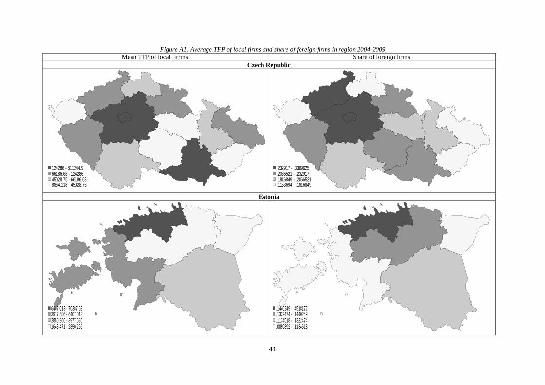
41

Figure A1: Average TFP of local firms and share of foreign firms in region 2004-2009 Mean TFP of local firrms Share of foreign firms

Czech Republic

Estonia

124286 - 811244.966186.68 - 12428645028.75 - 66186.688864.118 - 45028.75

.232917 - .3369625

.2066521 - .232917

.1816849 - .2066521

.1153694 - .1816849

6407.013 - 76387.683977.686 - 6407.0132850.266 - 3977.6861648.471 - 2850.266

.1440249 - .4518172

.1322474 - .1440249

.1134518 - .1322474

.0850892 - .1134518

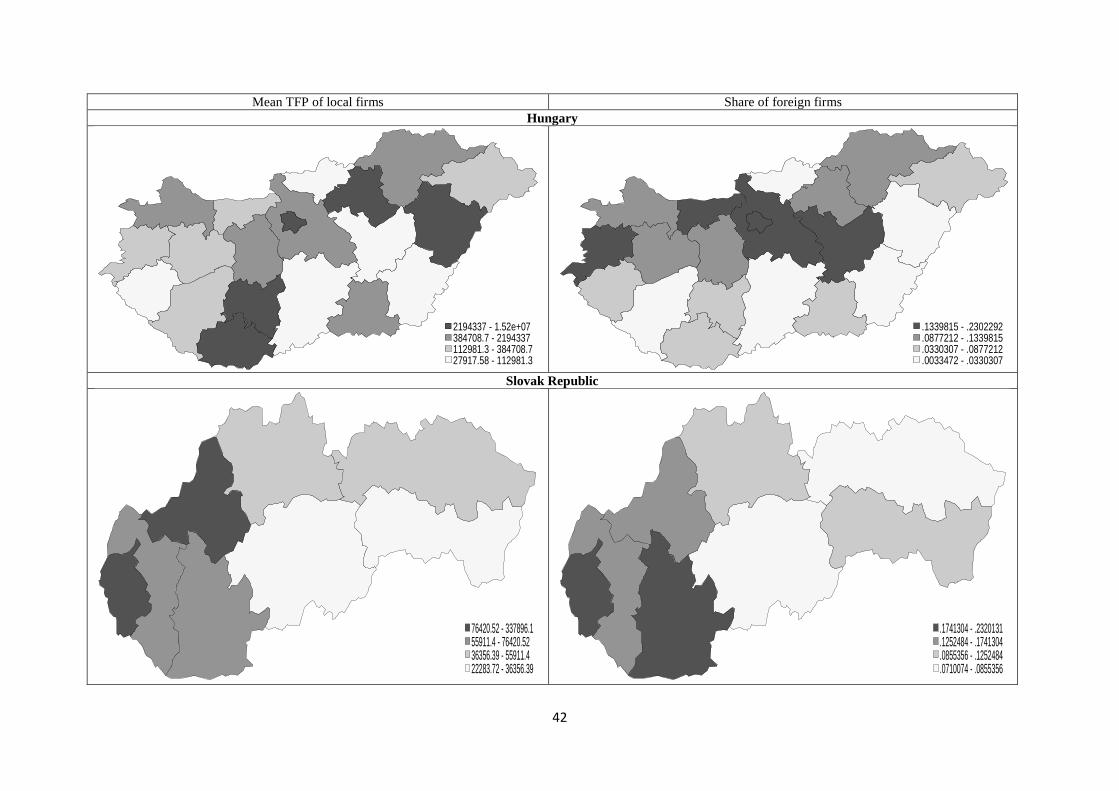
42

Mean TFP of local firms Share of foreign firms Hungary

Slovak Republic

2194337 - 1.52e+07384708.7 - 2194337112981.3 - 384708.727917.58 - 112981.3

.1339815 - .2302292

.0877212 - .1339815

.0330307 - .0877212

.0033472 - .0330307

76420.52 - 337896.155911.4 - 76420.5236356.39 - 55911.422283.72 - 36356.39

.1741304 - .2320131

.1252484 - .1741304

.0855356 - .1252484

.0710074 - .0855356

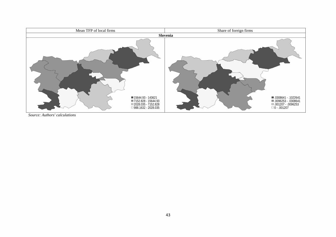
43

Mean TFP of local firms Share of foreign firms Slovenia

Source: Authors' calculations

15644.93 - 1436217152.828 - 15644.932028.035 - 7152.828988.1632 - 2028.035

.0308641 - .1022641

.0096253 - .0308641

.001207 - .00962530 - .001207

44