needs and means for a better workhorse trade model
DESCRIPTION
Needs and Means for a Better Workhorse Trade Model. Alan V. Deardorff University of Michigan Princeton Graham Lecture April 19, 2006. Introduction. The “workhorse models” of trade Partial equilibrium (for trade policies) Ricardian (for comparative advantage) - PowerPoint PPT PresentationTRANSCRIPT

Needs and Means for a Better Workhorse Trade Model
Alan V. Deardorff
University of Michigan
Princeton Graham Lecture
April 19, 2006

Graham Lecture 2
Introduction
• The “workhorse models” of trade– Partial equilibrium (for trade policies)– Ricardian (for comparative advantage)– Heckscher-Ohlin(-Samuelson) (HO) (for general
equilibrium effects of trade)– Krugman/Helpman-Krugman (HK) (for intra-industry
trade)
• Of these, the HO model has pride of place– Elegant but simple– Seemingly general, allowing extensions (e.g., HK) to
improve realism when needed

Graham Lecture 3
Introduction
• Uses of the HO model– As the core model for teaching general-
equilibrium trade• See Krugman-Obstfeld text, etc.
– As the main tool for understanding certain issues
• Trade of, and with, developing countries• “Trade and wages”
Graham Lecture 4
Introduction
• My reservations about the HO Model: some of its implications are– Extreme– Implausible– Inconvenient to take to data
• My hope for the HO Model: That it can be adapted, simply, to avoid these implications
Graham Lecture 5
Outline
• Some Uncomfortable Features of the H-O Model (The “Needs”)
• Assorted Potential Fixes (the “Means”)
• Elaboration of One of the Them: Increasing Trade Costs– How it meets the “needs”– Is it a good assumption?

Graham Lecture 6
Features of the HO Model
• What IS the HO Model?– Homogeneous goods and factors (any numbers > 1)– Perfectly competitive markets – Production functions
• Constant returns to scale• Non-joint
– Factors • Perfectly mobile across industries• Perfectly immobile across countries
– Countries differ in factor endowments– Industries differ in factor intensities– Trade costs, if present, are constant (perhaps
“iceberg”)
Graham Lecture 7
The “Needs”: Uncomfortable Features of the HO Model
• Factor Price Equalization• Too much trade, in both goods and factors• Indeterminacy of production and trade
(with more goods than factors, if prices align)
• Tendency to specialize (with more goods than factors, if prices don’t align)
• Hypersensitivity to prices and trade costs• Few equilibrium trade flows
Graham Lecture 8
The “Needs”: Uncomfortable Features of the HO Model
• Factor Price Equalization– This says: Under free and frictionless trade,
countries with sufficiently similar factor endowments will have exactly the same factor prices
– Implications:Insensitivity to own factor endowmentsOne-to-one sensitivity to foreign factor pricesNontraded goods prices determined entirely by
world prices of traded goods and not at all by nontraded good supplies or demands

Graham Lecture 9
The “Needs”: Uncomfortable Features of the HO Model
• Too much trade, in both goods and factor content– Trefler’s (1995) “Missing Trade”
Graham Lecture 10
The “Needs”: Uncomfortable Features of the HO Model
• Indeterminacy of production and trade (with more goods than factors, if prices align)

Graham Lecture 11
3-Good Lerner Diagram:Production Indeterminacy
L
K
Y=1/PY0
X=
1/P
X0
E0
X2
1/wK0
1/wL0
Z=1/PZ0
Y2X1
Z1

Graham Lecture 12
The “Needs”: Uncomfortable Features of the HO Model
• Tendency to specialize (with more goods than factors, if prices don’t align)– Countries have unequal factor prices and
therefore produce and trade at most 1 (or F−1) goods in common

Graham Lecture 13
3-Good Lerner Diagram:Two-Cone Model
L
K
Y=1/PY0
X=1/
P X0
1/wK2
1/wL2
Z=1/PZ0
1/wL1
1/wK1
Cone 1: Production of X and Y
Cone 2: Production of Y and Z

Graham Lecture 14
The “Needs”: Uncomfortable Features of the HO Model
• Implications of these more-goods-than-factors properties:Hypersensitivity to prices and trade costs of
production and (what countries) tradeHypersensitivity to tariff changes

Graham Lecture 15
Three-Good Lerner Diagram:Hypersensitivity
L
KX
Y
Z
E0
Small country facing FPE in rest of world with trade costs initially permitting import of 2 goods, Y and Z
Slight change in trade cost of any good can force output of either Y or Z to zero
Examples:
Rise in tZ forces import of Z to zero
Fall in tZ forces import of Y to zero

Graham Lecture 16
The “Needs”: Uncomfortable Features of the HO Model
• Hypersensitivity to prices and trade costs of (with whom countries) tradeHypersensitivity to preferential trading
arrangements

Graham Lecture 17
Geographic Hypersensitivity to Trade Costs
• Example:– 3 Countries, 2 goods– Country A is small
compared to both B and C
– B and C have zero trade costs between them
– A has trade costs with both B and C,
– but these may be different
B C
A

Graham Lecture 18
Geographic Hypersensitivity to Trade Costs
• Assume: • B and C identical, thus same autarky prices• A is capital abundant compared to B and C, so A has
comparative advantage in X
• Then:– A will trade based on 2×2 HO model, exporting X
and importing Y– With whom A trades depends on trade costs
• Let – TIJK be net export of good I from country J to country
K, and – tIJK be iceberg transport cost for that trade flow
Graham Lecture 19
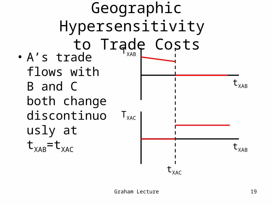
Geographic Hypersensitivity to Trade Costs
TXAC
tXAB
TXAB
tXAB
tXAC
• A’s trade flows with B and C both change discontinuously at tXAB=tXAC

Graham Lecture 20
The “Needs”: Uncomfortable Features of the HO Model
• Few equilibrium trade flowsNo intra-industry trade
Graham Lecture 21
Specialization
• With multiple countries, HO Model with trade costs predicts relatively few bilateral trade flows
• This cannot be seen in the 2×2×2 model, where so few are possible
• As number of countries C grows, number of possible bilateral trade flows grows with square of C. Maximum number of equilibrium trade flows in HO model (except with zero probability) grows only with C.
Graham Lecture 22
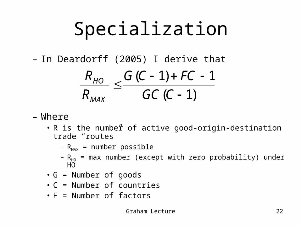
Specialization
– In Deardorff (2005) I derive that
– Where• R is the number of active good-origin-destination trade
“routes” – RMAX = number possible– RHO = max number (except with zero probability) under HO
• G = Number of goods• C = Number of countries• F = Number of factors
)1(
1)1(
CGC
FCCG
R
R
MAX
HO
Graham Lecture 23
Specialization
• Reason:– Each country will import each good only from
the lowest-cost source• One country, or• Group of countries whose prices and trade costs
align exactly for the importer. • If trade costs are random, on average the size of
such a group is limited by the number of factors.

Graham Lecture 24
The “Means”
• Ways to Make HO Behave?– Specific factors– Armington Preferences– Lumpy Countries– Monopolistic Competition– Heterogeneous Firms– Aggregation– Increasing Trade Costs

Graham Lecture 25
The “Means”
• Not a new question• CGE modelers have had to deal with it
– Models based too closely on HO don’t fit the data
– Most obviously (for me, via Bob Stern): Estimates of price elasticities of imports are much smaller than they would be in HO models taken literally
• due to “hypersensitivity”
– We’ve used several of the fixes mentioned here
Graham Lecture 26
Specific Factors
• Also called the Ricardo-Viner Model, this was how Samuelson (1971) and Jones (1971) got the HO Model to behave
• Each sector has its own “specific factor” = Factor that is either
• useless in, or • immobile to and from,
all other sectors

Graham Lecture 27
Specific Factors
• Implications– Supplies likely remain positive at all prices– Supplies increase smoothly with price– There is no indeterminacy– Trade does not equalize factor prices (Hence,
“Ohlin was right”)
Graham Lecture 28
Specific Factors
• Problems– Makes perfect sense for short run, but not for
long run– Doesn’t solve problem of hypersensitivity of
bilateral trade to trade costs– With specific factor in each industry, model no
longer “explains” trade, except tautologically: countries export products of their abundant specific factors

Graham Lecture 29
Armington Preferences
• Due to Armington (1969), who used it in a macroeconomic, not HO, context
• Products are differentiated by country of origin
• Examples?– French wine– Italian shoes– Swiss watches

Graham Lecture 30
Armington Preferences
• Implications– Trade need not equalize prices of same
“good” from different countries– Trade elasticities are much reduced
• hence all hypersensitivity is eliminated

Graham Lecture 31
Armington Preferences
• Problems– Trade now depends on preference
parameters as well as factor endowments• France exports wine because people like French
wine, etc.• (This is fine in CGE models, which don’t seek to
explain trade, but use trade data to inform trade policy)
– Preferences give every country market power in trade

Graham Lecture 32
Lumpy Countries
• Due to Courant and Deardorff (1992)
• Countries have multiple regions, across which there is not FPE

Graham Lecture 33
Lumpy Countries
• Implications– May alter pattern of trade from HO prediction– Internal regions may specialize– Regional limits on trade? Hence lower
elasticities?– Specialization at regional level without
specialization nationally? Hence less specialization?
– Continuum of regions?
Graham Lecture 34
Lumpy Countries
• Problems?– Don’t know yet– Hardly any of this has been worked out
Graham Lecture 35
Monopolistic Competition
• Helpman and Krugman (1985) put this in HO trade models, building on Spence-Dixit-Stiglitz preferences. Romalis (2004) generalized for empirical work
• Goods are differentiated by firm, while firm-level increasing returns limit product variety

Graham Lecture 36
Monopolistic Competition
• Implications– Most obviously, model explains intra-industry
trade– Implications for specialization and factor
prices are the same as the standard HO Model, so it does not help much with some of that
– Product-differentiated bilateral exports remain positive from any country that produces, avoiding hypersensitivity to trade costs

Graham Lecture 37
Monopolistic Competition
• Problems– Plausible for (some) manufactures and
services, but not for agricultural products, minerals, or some other inputs
– Doesn't change extremes of specialization

Graham Lecture 38
Heterogeneous Firms
• Melitz (2003) put this into trade theory, following Hopenhayn (1992). Bernard, Redding, and Schott (2005) put it in the HO model
• Individual firms each have a randomly chosen productivity parameter, as well as differentiated products

Graham Lecture 39
Heterogeneous Firms
• Implications– Industry gets small, but doesn’t disappear,
when factor prices move against it, since most productive firms survive
– Thus avoids extremes of specialization– Supply responds to prices through entry or
survival of less productive firms

Graham Lecture 40
Heterogeneous Firms
• Problems– Requires firm-level product differentiation as
well– Thus most appropriate only for manufactures– Not (yet?) particularly easy to use

Graham Lecture 41
Aggregation
• Davis and Weinstein (2001) suggest this in motivating part of their empirical work
• Observed industries are actually aggregates of unobservable industries with heterogeneous factor intensities

Graham Lecture 42
Aggregation
• Implications– Observed industries represent different mixes in
different countries, leading to cross-country correlation between factor endowments and factor intensities, even with FPE (Davis and Weinstein)
– In a multi-cone model, even though countries specialize in actual industries, observed industries operate at positive output due to products that unobservably belong to another cone
– In response to price changes, instead of a whole observed industry responding hypersensitively, only unobserved components do and observed industry responds gradually.
Graham Lecture 43
Aggregation
• Problems– This has not been worked out as a formal
model (I think)

Graham Lecture 44
Increasing Trade Costs
• I suggested in Deardorff (1984) that HO would be better behaved if trade costs varied appropriately
• Assume that trade costs for a particular good along a particular route (pair of countries) rise with the volume of trade
Graham Lecture 45
Increasing Trade Costs
• Implications– This makes bilateral export supply curves
upward sloping even when supplies of goods are infinitely elastic
– Indeterminacy of trade is eliminated– Volume of trade may then vary smoothly with
size of autarky price differences
Graham Lecture 46
Increasing Trade Costs
• Problems– Hard to imagine that this assumption could be
valid• If anything, transport seems more likely to have
decreasing costs, not increasing
• For now, I’ll ignore this problem and– Explore further the implications– Come back at the end to possible reasons for
rising trade costs

Graham Lecture 47
Increasing Trade Costs
• Assume:– HO model with rising, iceberg, trade costs– That is
• A fraction t of goods that are exported is used up in transit
• t increases with quantity exported, X: e.g.,
M = X(1-t) = X(1-cX)• (Could also include another component that is
positive for X=0, perhaps rising in distance.)

Graham Lecture 48
Implications of Increasing Trade Costs
• Small Country– Suppose it faces a single set of given prices,
pW, for goods delivered or purchased abroad• (Not now plausible in a world of many countries.
Prices will be different.)
– Compare to autarky prices, pA. • Trade pattern: as in HO, following factor-based
comparative advantage• Domestic prices, pD, move toward pW but do not
reach them, as t rises to offset |pW-pD|

Graham Lecture 49
Implications of Increasing Trade Costs
• Small Country Results– Trade pattern same as HO– But quantity of trade is less than HO– Goods prices drawn toward world prices, but
not to equality– Factor prices drawn toward world factor
prices, but also not to equality

Graham Lecture 50
Implications of Increasing Trade Costs
• Small Country Results– Factor price insensitivity
• No longer completely insensitive: Change in factor endowment changes both production/trade and factor price.
• Corollary of one-to-one sensitivity to foreign factor prices also dampened

Graham Lecture 51
Do Increasing Trade Costs (ITC)Meet the HO “Needs”?
• HO Need– Factor Price Equalization
• ITC– No FPE, only a tendency toward it

Graham Lecture 52
Do Increasing Trade Costs (ITC)Meet the HO “Needs”?
• HO Need– Factor Price Insensitivity to own factor
endowments
• ITC– Factor prices do respond to changing factor
endowments
Graham Lecture 53
Do Increasing Trade Costs (ITC)Meet the HO “Needs”?
• HO Need– One-to-one sensitivity to foreign factor prices
• ITC– Dependence on foreign factor prices is
reduced

Graham Lecture 54
Do Increasing Trade Costs (ITC)Meet the HO “Needs”?
• HO Need– Nontraded goods prices determined entirely
by world prices of traded goods and not at all by nontraded good supplies or demands
• ITC– Nontraded good supplies/demands affect
factor prices and thus nontraded good prices

Graham Lecture 55
Do Increasing Trade Costs (ITC)Meet the HO “Needs”?
• HO Need– Too much trade, in both goods and factors
• ITC– Trade is reduced, arbitrarily close to zero

Graham Lecture 56
Do Increasing Trade Costs (ITC)Meet the HO “Needs”?
• HO Need– Indeterminacy of production and trade (with
more goods than factors, if prices align)
• ITC– Indeterminacy eliminated, since production
and trade can’t change without changing prices
Graham Lecture 57
Do Increasing Trade Costs (ITC)Meet the HO “Needs”?
• HO Need– Tendency to specialize (with more goods than
factors, if prices don’t align)
• ITC– Specialization is unlikely, as it implies high
trade and thus high trade costs – (two countries with different factor prices can
produce many goods in common and trade, since variable trade costs makes up the difference in costs)

Graham Lecture 58
Do Increasing Trade Costs (ITC)Meet the HO “Needs”?
• HO Need– Hypersensitivity to prices and trade costs of
production and (what countries) trade
• ITC– Changes in prices and/or trade costs are
dampened by trade cost adjustment

Graham Lecture 59
Do Increasing Trade Costs (ITC)Meet the HO “Needs”?
• HO Need– Hypersensitivity to tariff changes
• ITC– Tariff cut expands imports which expands
trade cost to offset the tariff cut

Graham Lecture 60
Do Increasing Trade Costs (ITC)Meet the HO “Needs”?
• HO Need– Hypersensitivity to prices and trade costs of
(with whom countries) trade
• ITC– Hypersensitivity of trade partners reduced if
each has trade cost dependent on bilateral trade flow
Graham Lecture 61
Do Increasing Trade Costs (ITC)Meet the HO “Needs”?
• HO Need– Hypersensitivity to preferential trading
arrangements
• ITC– Preferential tariffs induce offsetting changes
in trade costs, dampening the response of trade

Graham Lecture 62
Do Increasing Trade Costs (ITC)Meet the HO “Needs”?
• HO Need– Few equilibrium trade flows
• ITC– More trade flows are likely, since countries
can import from and export to multiple partners, as trade costs offset price differences.
Graham Lecture 63
Do Increasing Trade Costs (ITC)Meet the HO “Needs”?
• HO Need– No intra-industry trade
• ITC– Does not yield intra-industry trade (unless
perhaps trade cost is negative for low trade!).

Graham Lecture 64
Do Increasing Trade Costs (ITC)Meet the HO “Needs”?
• Do Increasing Trade Costs provide a model that is simple enough to be a “workhorse”?– Perhaps not, in general– I suggest, therefore, an extreme version:
• Let trade costs rise for such small amounts of trade that effects on factor prices are negligible.
• Call it The Negligible Trade Model
Graham Lecture 65
Features of the Negligible Trade Model
• Factor Prices are approximately those of autarky• Trade depends, via variable trade costs, on
relative autarky prices• Small effects of trade on factor prices and other
variables can be obtained by differentiation from initial autarky equilibrium
• Trade flows depend fairly simply on factor endowments

Graham Lecture 66
Implication of Increasing Trade Costs
• Implies that even a small country faces diminishing terms of trade.
• Thus even small country’s optimal tariff > 0!
• Reason: rising trade cost is an externality. X
Y
O
B
B′
A
Trade Cost

Graham Lecture 67
Possible Reasons for Increasing Trade Costs
• Congestion
• Trade-specific factors and/or capacity constraints (Coleman 2005)
• Cost of market penetration (geographic or other)

Graham Lecture 68
Conclusion
• Increasing trade costs are worth looking into– Use trade flow equation to estimate
relationship of trade costs to trade– If successful, explore more fully the various
reasons for increasing trade costs

Graham Lecture 69
Acknowledgements
• Thanks, for their input, to– Gene Grossman– Juan Carlos Hallak– Bob Stern– Jim Tybout

Graham Lecture 70
References• Armington, Paul S. 1969 "A Theory of Demand for Products Distinguished by Place of Production," IMF
Staff Papers 16, (March), pp. 159-178.• Bernard, Andrew B., Stephen Redding, and Peter Schott 2004 “Comparative Advantage and
Heterogeneous Firms,” Institute for Fiscal Studies, IFS Working Paper: W04/24.• Coleman, Andrew 2005 “Have We Misunderstood the Law of One Price? A Reinterpretation based on a
Trade Model with Transport Capacity Constraints,” August 23, University of Michigan.• Courant, Paul N. and Alan V. Deardorff 1992 "International Trade with Lumpy Countries," Journal of
Political Economy 100, (February), pp. 198-210.• Davis, Donald R. and David E. Weinstein 2001 “An Account of Global Factor Trade,” American
Economic Review 91(5), (December), pp. 1423-1453.• Deardorff, Alan V. 1984 "Testing Trade Theories and Predicting Trade Flows," in Ronald Jones and Peter
Kenen, eds., Handbook of International Economics Volume 1, New York: North Holland, Chapter 10.• Deardorff, Alan V. 2005 “The Heckscher-Ohlin Model: Features, Flaws, and Fixes,” Nottingham
Lectures, October 17-18, 2005• Helpman, Elhanan and Paul R. Krugman 1985 Market Structure and Foreign Trade: Increasing Returns,
Imperfect Competition, and the International Economy, Cambridge, MA: MIT Press.• Jones, Ronald W. 1971 "A Three Factor Model in Theory, Trade, and History," in J.N. Bhagwati, R.W.
Jones, R.A. Mundell, and J. Vanek, eds., Trade, Balance of Payments, and Growth: Essays in Honor of Charles P. Kindleberger, Amsterdam: North Holland.
• Melitz, Marc 2003 “The Impact of Trade on Intra-industry Reallocations and Aggregate Industry Productivity,” Econometrica 71(6), (November), pp. 1695-1725.
• Romalis, John 2004 “Factor Proportions and the Structure of Commodity Trade,” American Economic Review 94(1), (March), pp. 67-97.
• Samuelson, Paul A. 1971 "Ohlin Was Right," Swedish Journal of Economics 73, pp. 365 384.• Trefler, Daniel 1995 "The Case of the Missing Trade and Other Mysteries," American Economic Review
85, (December), pp. 1029-1046.