neighborhood effects and trial on the internet: evidence from online grocery retailing ·...
TRANSCRIPT
Quant Market Econ (2007) 5:361–400DOI 10.1007/s11129-007-9025-5
Neighborhood effects and trial on the Internet:Evidence from online grocery retailing
David R. Bell · Sangyoung Song
Received: 21 March 2006 / Accepted: 8 March 2007 /Published online: 23 August 2007© Springer Science + Business Media, LLC 2007
Abstract For traditional retailers the customer pool is largely bounded inspace, whereas an Internet retailer can obtain customers from a wide geo-graphical area. We examine customer trials at Netgrocer.com, and drawingon studies in marketing and economics conjecture that exposure spatially toproximate others (through direct social interaction or observation), can influ-ence decisions of those who have yet to try. Trials arise from utility-maximizingbehavior and the model is estimated as a discrete time hazard. The data span:(1) 29,701 residential zip codes, (2) 45 months of transactions since inception,and (3) zip code contiguity relationships. The estimated neighborhood effectis significantly positive and economically meaningful.
Keywords Discrete time hazard · Neighborhood effect · Random utility ·Retailing
JEL Classification C25 · M30
D. R. Bell (B)The Wharton School, University of Pennsylvania,700 Huntsman Hall, 3730 Walnut Street, Philadelphia, PA 19104, USAe-mail: [email protected]
S. SongThe Zicklin School of Business, Baruch College,1 Bernard Baruch Way, New York, NY 10010, USAe-mail: [email protected]
362 D. R. Bell, S. Song
“. . . The choice of a store location has a profound effect on the entirebusiness life of a retail operation. A bad choice may all but guaranteefailure, a good choice, success.”
“Store Location: Little Things Mean A Lot” CBSC, Government ofCanada.
For retailers “location, location, location” is a familiar mantra and a vast lit-erature substantiates its importance. While pricing and assortment are criticalas well location accounts for the most variation in outlet choice in many retailsettings.1 For an e-tailer, physical location of the store relative to potentialcustomers is no consequence. Indeed, the trading area of the e-retailer isconstrained only by the availability of shipment infrastructure for distributingorders. The location of existing customers relative to potential customers andtheir interactions, may however be critical.
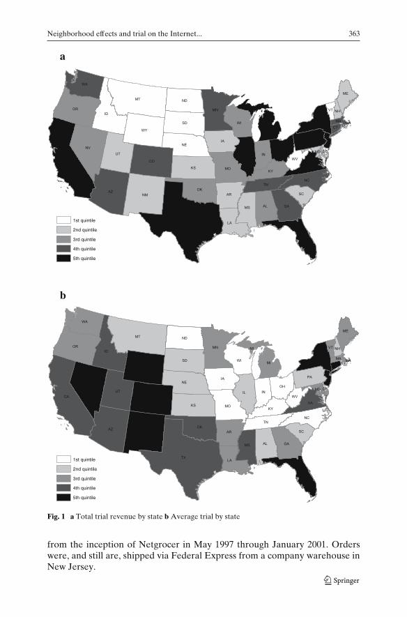
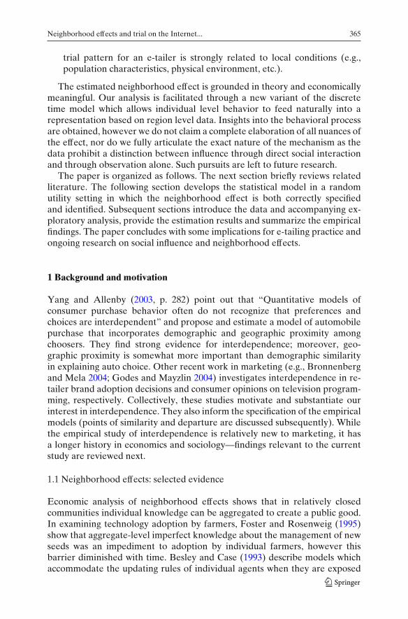
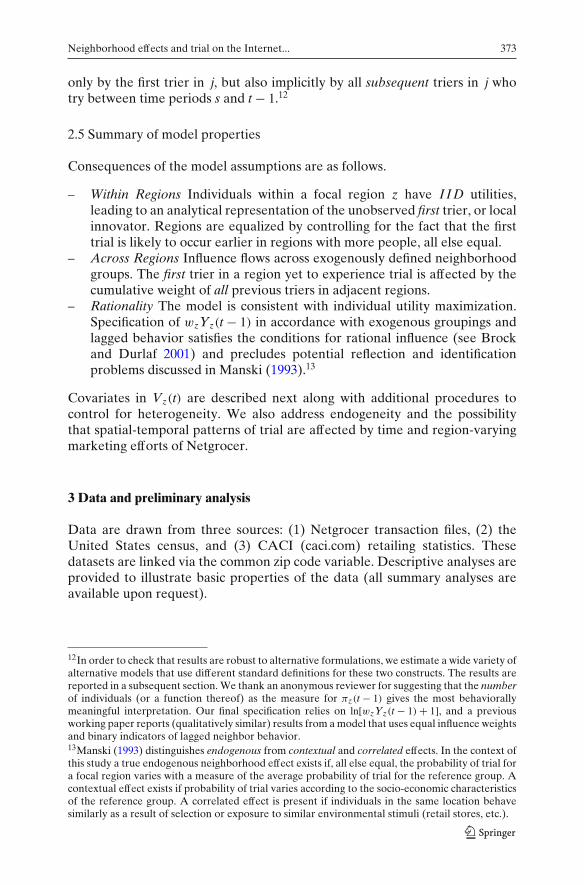
An e-tailer’s unique market context—geographically dispersed customersand competitors—raises important (and thus far unstudied) questions aboutthe evolution of the customer base. The role of existing customers in recruitingor influencing new potential customers is especially fundamental. Emulation indecision making has been studied in theoretical and empirical research in eco-nomics and sociology (e.g., Burt 1980; Goolsbee and Klenow 2002; Tolnay et al.1996; Van den Bulte and Lilien 2001) and is the focus of our research. We areuniquely positioned to address this issue in an e-tail setting through the space-time evolution of trials from the inception of a new Internet grocery retailer.A descriptive characterization of the data motivates the modeling frameworkand underlying theory. Figure 1 summarizes trial orders for Netgrocer withtotal revenue earned and average order value by state shown in panels (a) and(b), respectively.
The empirical distribution of these two variables is broken into quintiles.2
California, Texas, Florida and New York generate the greatest amount ofrevenue, while the average order values are higher in the interior westernstates of Nevada, Wyoming, Colorado and New Mexico. Population size isa likely explanation for the first observation, while the second may resultfrom greater travel distances to retail services. The important fact is that thecustomer base spans the entire United States. The data in Fig. 1 are cumulative
1For example, Progressive Grocer (April 1995) reports that location explains up to 70% of thevariance in consumer choice of supermarket retailers. Moreover, the attractiveness of an outlet toa shopper declines exponentially the further the individual is from the store (e.g., Fotheringham1988; Huff 1964).2For reasons of confidentiality we have excluded the dollar values from panel (a), however all 48contiguous states generate revenue.
Neighborhood effects and trial on the Internet... 363
b
a
TX
CA
MT
AZ
ID
NV
NM
CO
IL
OR
UT
KS
WY
IA
SD
NE
MN
FL
ND
OK
WI
MO
AL
WA
GA
LA
AR
MI
IN
NC
NY
PA
MS
TN
KY
VA
OH
SC
ME
WV
MI VT NH
MD
NJ
MA
CT
DE
RIMA
RI
1st quintile
2nd quintile
3rd quintile
4th quintile
5th quintile
TX
CA
MT
AZ
ID
NV
NM
CO
IL
OR
UT
KS
WY
IA
SD
NE
MN
FL
ND
OK
WI
MO
AL
WA
GA
LA
AR
MI
IN
NC
NY
PA
MS
TN
KY
VA
OH
SC
ME
WV
MI VT NH
MD
NJ
MA
CT
DE
RIMA
RI
1st quintile
2nd quintile
3rd quintile
4th quintile
5th quintile
Fig. 1 a Total trial revenue by state b Average trial by state
from the inception of Netgrocer in May 1997 through January 2001. Orderswere, and still are, shipped via Federal Express from a company warehouse inNew Jersey.
364 D. R. Bell, S. Song
For the remainder of the paper we focus on the spread of initial orders overtime and space, with special emphasis on social influence or “neighborhoodeffects” in speeding up or inhibiting the process.3 Studies in economics andsociology (e.g., Bikhchandani et al. 1998; Case 1991; Case et al. 1989; Singerand Spilerman 1983) motivate our representation of neighborhood effects,however marketing researchers are also beginning to analyze spatial aspectsof diffusion processes (see for example, Bronnenberg and Mela 2004; Garberet al. 2004). We propose and estimate a model in which trial decisions resultfrom utility-maximizing behavior. Trial is observed when an individual-specificthreshold for action is exceeded. The advantage of this conceptualization isthat a time-dependent process can be examined through a sequence of binaryactions.4
Contribution and caveats
We demonstrate empirically the importance of neighborhood effects in gen-erating trial at an Internet grocery retailer. The substantive message is in linewith Goolsbee and Klenow (2002) who find that individuals are more likelyto buy home computers in areas where greater numbers of other individualsalready own computers. We find similar neighborhood effects, given simplerepresentations of influence derived from physical proximity. The estimatedeffect is economically and statistically important and is robust to controls forregion and time-specific fixed effects, region covariates, unobserved hetero-geneity in the baseline hazard, and alternative specifications for access to theInternet. We contribute the following:
– First, we develop a framework for empirical analysis of a new phenomenonin retailing, namely the evolution of customer trials for an e-tailer. Inso doing, we provide insight into the consequences of spatially dispersedcustomers and competitors.
– Second, we offer an analytical derivation to estimate parameters of aninherently individual-level decision process using region-level data. Therelationship between random utility maximization and a discrete timehazard model coupled with knowledge of the number of individuals ineach region accomplishes this. Our approach avoids individual-level co-variates, unrealistic assumptions about right censoring, and problems inexogenously defining neighbor relationships.
– Third, we find that neighborhood effects influence the “private behavior”of e-tailer trial, and are economically important. Moreover, the space-time
3The former term is preferred by sociologists and the latter by economists, but have complemen-tary interpretations: Neighborhood effects emanate from the influence of well-defined exogenousgroups on a focal group, whereas social influence refers to the broader behavioral process.We focus on an empirically grounded neighborhood effect without speculation as to the exactmechanism.4Specifically, a discrete time hazard model estimated on time-dependent trial data is consistentwith random utility maximization over binary outcomes.
Neighborhood effects and trial on the Internet... 365
trial pattern for an e-tailer is strongly related to local conditions (e.g.,population characteristics, physical environment, etc.).
The estimated neighborhood effect is grounded in theory and economicallymeaningful. Our analysis is facilitated through a new variant of the discretetime model which allows individual level behavior to feed naturally into arepresentation based on region level data. Insights into the behavioral processare obtained, however we do not claim a complete elaboration of all nuances ofthe effect, nor do we fully articulate the exact nature of the mechanism as thedata prohibit a distinction between influence through direct social interactionand through observation alone. Such pursuits are left to future research.
The paper is organized as follows. The next section briefly reviews relatedliterature. The following section develops the statistical model in a randomutility setting in which the neighborhood effect is both correctly specifiedand identified. Subsequent sections introduce the data and accompanying ex-ploratory analysis, provide the estimation results and summarize the empiricalfindings. The paper concludes with some implications for e-tailing practice andongoing research on social influence and neighborhood effects.
1 Background and motivation
Yang and Allenby (2003, p. 282) point out that “Quantitative models ofconsumer purchase behavior often do not recognize that preferences andchoices are interdependent” and propose and estimate a model of automobilepurchase that incorporates demographic and geographic proximity amongchoosers. They find strong evidence for interdependence; moreover, geo-graphic proximity is somewhat more important than demographic similarityin explaining auto choice. Other recent work in marketing (e.g., Bronnenbergand Mela 2004; Godes and Mayzlin 2004) investigates interdependence in re-tailer brand adoption decisions and consumer opinions on television program-ming, respectively. Collectively, these studies motivate and substantiate ourinterest in interdependence. They also inform the specification of the empiricalmodels (points of similarity and departure are discussed subsequently). Whilethe empirical study of interdependence is relatively new to marketing, it hasa longer history in economics and sociology—findings relevant to the currentstudy are reviewed next.
1.1 Neighborhood effects: selected evidence
Economic analysis of neighborhood effects shows that in relatively closedcommunities individual knowledge can be aggregated to create a public good.In examining technology adoption by farmers, Foster and Rosenweig (1995)show that aggregate-level imperfect knowledge about the management of newseeds was an impediment to adoption by individual farmers, however thisbarrier diminished with time. Besley and Case (1993) describe models whichaccommodate the updating rules of individual agents when they are exposed

366 D. R. Bell, S. Song
to knowledge transmission by others. Case et al. (1993) find that publicspending in a particular region is strongly influenced by levels of expenditure inneighboring jurisdictions (for every one dollar spent by a contiguous neighboran additional seventy cents is spent by the focal region). Moreover, failureto account for this in estimation leads to an upwards bias in other modelparameters.
Sociologists have also contributed a number of insights. Many studies focuson social connectedness and the extent of information transfer among andbetween groups of individuals (see Burt 1980 for a comprehensive treatment;also Greve et al. 1995; Strang and Tuma 1993). While social contagion can begrounded primarily in geographical contiguity, sociologists have also examinedthe structure of interpersonal affiliation. Burt (1980) discusses social cohesionand related studies describe how an affiliation matrix can be constructed tocapture the nature, strength and timing of interaction within groups. Chaves(1996) for example, shows that the diffusion of gender equality in churchesis influenced by cultural boundaries and affiliations within the denominationsstudied.
The power of social contact in information dissemination is demonstratedin a clever study by Oyen and De Fleur (1953). In a field experiment leafletswere distributed by plane over four areas of Washington state. Knowledge ofthe message content by individual discovery was found to decline dramaticallywith increased distance from the drop areas, while knowledge via social contact(i.e., learning the content from others) tended to increase within the circum-scribed distance. Finally, it is important to keep in mind that observationallearning can induce both negative and positive dispositions with respect to theinnovation. Tolnay et al. (1996) study state-tolerated racist violence in the USat the turn of the century and report that the number of lynchings occurring ina particular county decreased with the number of prior lynchings in contiguousneighbors. That is, contagion effects can be negative (i.e., slow the spread ofthe phenomenon) as well as positive.
1.2 Neighborhood effects: conceptualization and measurement
A longstanding tradition in marketing posits a generic consumer decisionmaking process in which an individual passes through discrete stages in anapproximately linear fashion. Lilien et al. (1993, p. 26) describe a five stageprocess: need arousal, information search, evaluation, purchase and postpurchase. Each stage differs with respect to sources and use of information,time taken, and decision rules invoked and applied.5
Our model focuses exclusively on a single stage (trial) and incorporatesimportant elements suggested by prior literature. Trials arise because unob-served utility thresholds have been crossed, and new information is potentiallyrevealed to current non-triers as a consequence of trial by proximate others. Toproperly investigate how the trial behavior of spatially proximate neighbors
5This conceptualization can be traced back to early work by Howard and Sheth (1969).

Neighborhood effects and trial on the Internet... 367
affects current non-triers we require exogenous definitions of groups andneighborhood relationships.6 In our application neighborhood relationshipsare known at the level of the region (zip code) but not at the level of theindividual. We know the exact spatial proximity of different zip codes, butnothing about relative locations of individuals residing in the same zip code.Moreover, no individual-level covariate information is available for eithertriers or non-triers. Thus, the pattern of social influence, or neighborhoodeffect, will be specified empirically as a region-to-region phenomenon. We donot however ignore the potential for influence that occurs among individualswho share a specific region, rather we separate out the within and across regionpossibilities for transmission of information and emulation of triers by non-triers. The motivation for this conceptualization stems from the institutionalsetting, the data, and from the studies referenced above. The next sectionpresents a model based on random utility maximization that incorporates allthese elements in an integrated way.
In summary, theories in economics and sociology motivate why new triersof an Internet service could be influenced by existing users who are spatiallyproximate. In addition, recent empirical work in marketing highlights thepresence of neighborhood effects in a variety of contexts (brand adoptionby retailers, auto purchases by consumers, television viewership). Our studyextends the set of contexts to include the Internet. Moreover, we exploit therelationship between random utility models and discrete time hazard models tooffer a method that allows examination of neighborhood effects in the absenceof strictly individual level data. Neighborhood effects are modeled as a directcovariate (Bronnenberg and Mela 2004; Goolsbee and Klenow 2002), ratherthan through an auto-regressive error structure (Yang and Allenby 2003).
2 Empirical model
We motivate the statistical model by highlighting the link between individualutility maximization for time-dependent binary choices and a discrete timehazard model. Moreover, we show our discrete time formulation estimatesthe parameters of an underlying continuous time proportional hazards model.The hazard model imposes three important requirements on the data: (1)exact knowledge of the risk set (those observational units yet to experiencetrial) at each time period, (2) covariate information for all risk set members,and (3) exact knowledge of neighbor relationships in order to identify theneighborhood effect. A full individual level model would therefore requirevery detailed covariate data on 300 million individuals and information onwhere they live in relation to each other. This requirement is clearly impossibleto meet. We therefore derive a model based on region level data which satisfies(1)–(3) above, yet is consistent with individual-level decision making.
6For a complete treatment of this issue see Anselin (1988) and Manski (1993).
368 D. R. Bell, S. Song
2.1 Individual utility for trial
Consider trial decisions for individuals located in regions z = 1, . . . , Z and letTiz denote the uncensored time of occurrence of trial for individual i. To allowa behavioral underpinning (utility maximization) for individual trial decisions,we work with the discrete time hazard
Piz(t) = P(Tiz = t|Tiz ≥ t, Xiz(t)). (1)
Xiz(t) are covariates that potentially influence the uncensored time of trial.Equation 1 is the conditional probability that an event occurs at t, giventhat it has yet to occur, and can result from a model of random utilitymaximization over binary choices. Furthermore, it is important to note thata discrete time model need not result in a loss of information nor be subject toaggregation bias. Specifically, discrete time parameter estimates derived fromthe complementary log-log link function are also the estimates of an underlyingcontinuous time proportional hazards model (Prentice and Gloeckler 1978).7
In addition to the substantive advantage of a utility interpretation offered bythe discrete time approach, methodological benefits are simplicity of estima-tion and the ability to incorporate time-varying covariates. Allow individual iin region z the potential for in trial in any period t, beginning at period 1 (whenthe innovation first becomes available). The observed variable yiz(t) ∈ {0, 1}indicates that the individual experienced trial (yiz(t) = 1) or not (yiz(t) = 0).The complete decision history is described by the time-indexed sequence{yiz(t)}, t = 1, . . . , Tiz ≤ T where Tiz is the time period in which trial takesplace for individual i. If trial never occurs, {yiz(t)} is a sequence of zeros oflength T (the end of the observation period).
To see the link to random utility maximization, assume individual i atlocation z has a latent utility for trial at time t
Uiz(t) = Viz(t) − εiz(t), (2)
where Viz(t) is a linear in parameters polynomial sum and εiz(t) a stochasticdisturbance. In general, Viz(t) potentially depends on individual, region andtime-dependent characteristics; the probability distribution of εiz(t) governsthe relationship between Viz(t) and yiz(t).
2.2 An individual model with region level data
With complete individual-level covariate information one could estimate theparameters of Eq. 2. As noted previously, the data requirements would be
7Please see Appendix. Parameters of discrete time models are usually not invariant to the lengthof time intervals chosen (Heckman and Singer 1984a; Ryu 1995); the discrete time model withcomplementary log-log link function is the exception (see also Allison (2001 p. 216-219.). TerHofstede and Wedel (1999) document aggregation biases in discrete time models. Ryu (1995)shows that even for a standard discrete time model a time interval to average event time ratio of1/16 is generally sufficient to mitigate bias.

Neighborhood effects and trial on the Internet... 369
enormous. It is therefore impossible to specify Viz(t) in Eq. 2 at the individuallevel of aggregation directly. We now derive a region level model which allowsidentification of the risk set, and covariates for set members. The region levelmodel also enables us to specify neighborhood relationships exogenously.Finally, right censoring is less problematic as it is reasonable to assume thatgiven enough time, each zip code will see at least one trial.8
At the individual level trial occurs when the utility threshold is crossed.Namely, yiz(t) = 1 when Uiz(t) > τ where τ can be normalized to zero withoutloss of generality. Let εiz(t) be independently and identically distributed overindividuals and time within region
f (ε) = 1
μexp
[ε − η
μ
]exp
{−e
ε−η
μ
}. (3)
The probability that individual i in region z experiences trial at time t isobtained as
P(yiz(t) = 1) = P(εiz(t) ≤ Viz(t)) = Fε(Viz(t))
= 1 − exp
{− exp
{Viz(t) − η
μ
}}. (4)
For reasons given above, we do not model this probability but instead modelthe probability of the first trial in a region. The probability that trial occurs inregion z at time t, given that trial has yet to occur there is equivalent to theprobability that the utility of the maximal individual exceeds the threshold.Note that while this maximal individual cannot be described in terms ofindividual-level characteristics, s/he can be represented by a combinationof region-specific characteristics and the implied individual-level stochasticcomponent of utility. That is
P(yz(t) = 1) = P( maxi
{ Uiz(t) i = 1, . . . , nz } ≥ 0)
= P( maxi
{ Viz(t) − εiz(t) } ≥ 0)
= P( Vz(t) − mini
{ εiz(t) } ≥ 0)
since we have Viz(t) = Vz(t) ∀i
= P( mini
{ εiz(t) } ≤ Vz(t)). (5)
Equation 5 reframes the event—trial in region z at time t—with respect tothe distribution of the minimum of i = 1, . . . , nz random variables. In words,the probability that the unobserved maximal individual’s utility exceeds zero
8It is much less reasonable to assume that given enough time each individual will eventually tryNetgrocer.

370 D. R. Bell, S. Song
is equivalent to the probability that the observed deterministic utility Vz(t) forthe representative individual from the region exceeds the minimum value ofall εiz(t). It is worthwhile to reflect on the statistical and behavioral appeal andconsequences of this I I D assumption. The I I D assumption implies that thereis no within region contagion for the first trial which is not unreasonable.9
The Gumbel distribution in Eq. 3 with location parameter η and scaleparameter μ has the useful property that the distribution of the minimum ofnz independent random variables is also Gumbel
εiz(t) ∼ G(η, μ)
εminz (t) = min
i{ εiz, i = 1, . . . , nz}
∼ G(η − μln(nz), μ). (6)
Setting η = 0 and μ = 1 as standard normalizations, the probability that trialoccurs in region z given that it has not yet occurred is
P(yz(t) = 1) = Fminε (Vz(t))
= 1 − exp
{− exp
{Vz(t) − (η − μ ln(nz))
μ
}}
= 1 − exp {− exp {Vz(t) + ln(nz)}} . (7)
Intuitively, the more individuals there are in a region, the greater the chancethat at least one will experience trial by a particular date. When combiningdata across regions, it is vital to take this into account. ln(nz) is thereforean “offset” factor controlling for the fact trial is more likely to be observedearlier in regions containing more individuals. In practical empirical termsnz is simply the region population and easily obtained from the census. Theinclusion of ln(nz) in the probability expression is not arbitrary but arises froma specific model of individual behavior. As shown in the Appendix, Eq. 7 is alsoa complementary log-log link function and therefore estimates an underlyingcontinuous time proportional hazards model.
Equation 7 does not yet include a neighborhood effect covariate, whichwill be specified subsequently. Arrival at a region level specification whereneighbor relations are exogenously known makes it possible to investigateneighborhood effects (or region-to-region influence) in trial. At the same time,
9Conceptually, this says that first individual to try in a region was a “local innovator” and notinfluenced by others in the region. This is behaviorally plausible because none of the other same-region individuals had in fact tried. At the same time, the model will however allow for the firsttrier in region z to be influenced by prior triers in region j, if region j is a neighbor of z. Detailsfollow shortly.
Neighborhood effects and trial on the Internet... 371
the model will allow the first trier in region z to be influenced by prior triers inregion j, if region j is a contiguous neighbor of region z.
2.3 Accounting for region level heterogeneity
The derivation above preserves an individual-level behavioral interpretationeven though the model will be estimated using region level data. It also servesa statistical purpose because it implies region-level variation in the baselinehazard. To see this, assume that the region-level utility Vz(t) (not including theoffset) is equal to αz + β Xz(t), where Xz(t) contains region and time-varyingcovariates to be specified shortly. We have
Vz(t) = αz + β Xz(t) + ln(nz) (8)
= α0 + β Xz(t) + ln(nz) + (αz − α0)︸ ︷︷ ︸= α0 + β Xz(t) + φ ln(nz)
where φ = ln(nz) + (αz − α0)
ln(nz)(9)
Hence, when pooling data across regions imposing the theoretical constraintφ = 1 in Eq. 7 is equivalent to assuming that αz = α0 (in the absence of anadditional random term in Eq. 8). This is unlikely to be true empirically so weallow a free parameter for the offset term and model the intercept as a randomeffect (see also Appendix for details)
Vz(t) = αz + β Xz(t) + φ ln(nz), αz = α0 + νz νz ∼ N(0, σ 2). (10)
The model exhibits the appealing property that the control for heterogeneityfalls naturally out of the derivation, which in turn follows directly from anunderlying behavioral model.10
2.4 Neighborhood effects
Imagine that in a region where no individual has yet tried, there is potential foreither direct communication with, or passive observation of, individuals froman adjacent region where trial has occurred.11 As an illustration, consider twoadjacent regions, z1 and z2 and imagine trial occurs in region z1 at t − 1. Ifindividuals in z2 gain knowledge of the event {yz1(t − 1) = 1}, this may lead toa change in the conditional probability of trial in z2 where the conditioning is
10We also estimate Vz(t) = αz + β Xz(t) + ln(nz), αz = α0 + ηz ηz ∼ N(0, σ 2). Results are dis-cussed in the next section.11As noted earlier, we do not distinguish between the two. Passive observation is facilitated byindividuals observing deliveries (each box is clearly marked with “netgrocer.com”). Unfortunately,we cannot address Internet-based communication directly as we have no way to track it.
372 D. R. Bell, S. Song
now on the prior event in z1 such that P(yz2(t) = 1|yz1(t − 1) = 1) �= P(yz2(t) =1|yz1(t − 1) = 0). This notion is reflected in the deterministic utility
V ′z(t) = Vz(t) + θ [wzYz(t − 1)], (11)
where wz is a row vector whose elements capture the relationship betweenregion z and its neighbors. It has dimension 1 × Nz where Nz equals thenumber of neighbors in the neighborhood set, including z itself. Yz(t − 1) isan Nz × 1 column vector of the lagged trial behavior of individuals who residein zip codes contained in the neighborhood set.
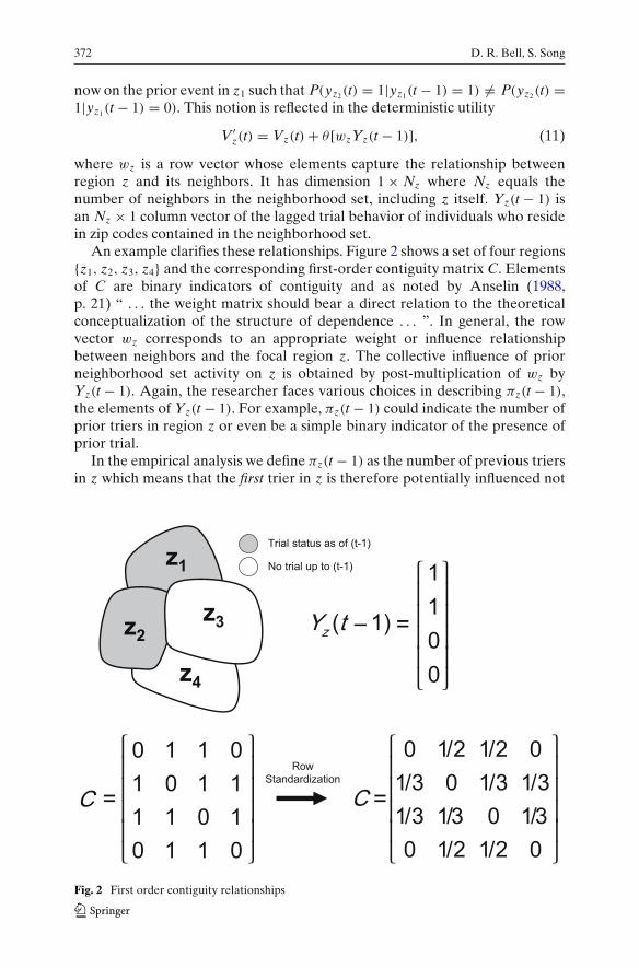
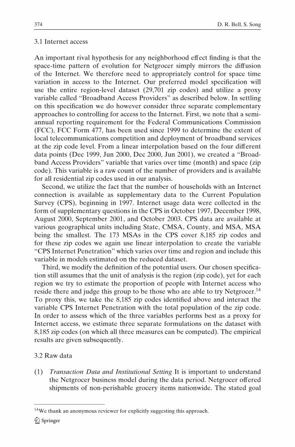
An example clarifies these relationships. Figure 2 shows a set of four regions{z1, z2, z3, z4} and the corresponding first-order contiguity matrix C. Elementsof C are binary indicators of contiguity and as noted by Anselin (1988,p. 21) “ . . . the weight matrix should bear a direct relation to the theoreticalconceptualization of the structure of dependence . . . ”. In general, the rowvector wz corresponds to an appropriate weight or influence relationshipbetween neighbors and the focal region z. The collective influence of priorneighborhood set activity on z is obtained by post-multiplication of wz byYz(t − 1). Again, the researcher faces various choices in describing πz(t − 1),the elements of Yz(t − 1). For example, πz(t − 1) could indicate the number ofprior triers in region z or even be a simple binary indicator of the presence ofprior trial.
In the empirical analysis we define πz(t − 1) as the number of previous triersin z which means that the first trier in z is therefore potentially influenced not
z1
z2
z3
z4
Row
Standardization
0 1 1 0
1 0 1 1
1 1 0 1
0 1 1 0
C
0 1/2 1/2 0
1/3 0 1/3 1/3
1/3 1/3 0 1/3
0 1/2 1/2 0
C
Trial status as of (t-1)
No trial up to (t-1) 1
1( 1)
0
0
zY t –
⎫
⎭⎪⎪⎪⎪
⎧
⎩⎪⎪⎪⎪
⎫
⎭⎪⎪⎪⎪
⎧
⎩⎪⎪⎪⎪
⎫
⎭⎪⎪⎪⎪
⎧
⎩⎪⎪⎪⎪
= =
=
Fig. 2 First order contiguity relationships
Neighborhood effects and trial on the Internet... 373
only by the first trier in j, but also implicitly by all subsequent triers in j whotry between time periods s and t − 1.12
2.5 Summary of model properties
Consequences of the model assumptions are as follows.
– Within Regions Individuals within a focal region z have I I D utilities,leading to an analytical representation of the unobserved first trier, or localinnovator. Regions are equalized by controlling for the fact that the firsttrial is likely to occur earlier in regions with more people, all else equal.
– Across Regions Influence flows across exogenously defined neighborhoodgroups. The first trier in a region yet to experience trial is affected by thecumulative weight of all previous triers in adjacent regions.
– Rationality The model is consistent with individual utility maximization.Specification of wzYz(t − 1) in accordance with exogenous groupings andlagged behavior satisfies the conditions for rational influence (see Brockand Durlaf 2001) and precludes potential reflection and identificationproblems discussed in Manski (1993).13
Covariates in Vz(t) are described next along with additional procedures tocontrol for heterogeneity. We also address endogeneity and the possibilitythat spatial-temporal patterns of trial are affected by time and region-varyingmarketing efforts of Netgrocer.
3 Data and preliminary analysis
Data are drawn from three sources: (1) Netgrocer transaction files, (2) theUnited States census, and (3) CACI (caci.com) retailing statistics. Thesedatasets are linked via the common zip code variable. Descriptive analyses areprovided to illustrate basic properties of the data (all summary analyses areavailable upon request).
12In order to check that results are robust to alternative formulations, we estimate a wide variety ofalternative models that use different standard definitions for these two constructs. The results arereported in a subsequent section. We thank an anonymous reviewer for suggesting that the numberof individuals (or a function thereof) as the measure for πz(t − 1) gives the most behaviorallymeaningful interpretation. Our final specification relies on ln[wzYz(t − 1) + 1], and a previousworking paper reports (qualitatively similar) results from a model that uses equal influence weightsand binary indicators of lagged neighbor behavior.13Manski (1993) distinguishes endogenous from contextual and correlated effects. In the context ofthis study a true endogenous neighborhood effect exists if, all else equal, the probability of trial fora focal region varies with a measure of the average probability of trial for the reference group. Acontextual effect exists if probability of trial varies according to the socio-economic characteristicsof the reference group. A correlated effect is present if individuals in the same location behavesimilarly as a result of selection or exposure to similar environmental stimuli (retail stores, etc.).
374 D. R. Bell, S. Song
3.1 Internet access
An important rival hypothesis for any neighborhood effect finding is that thespace-time pattern of evolution for Netgrocer simply mirrors the diffusionof the Internet. We therefore need to appropriately control for space timevariation in access to the Internet. Our preferred model specification willuse the entire region-level dataset (29,701 zip codes) and utilize a proxyvariable called “Broadband Access Providers” as described below. In settlingon this specification we do however consider three separate complementaryapproaches to controlling for access to the Internet. First, we note that a semi-annual reporting requirement for the Federal Communications Commission(FCC), FCC Form 477, has been used since 1999 to determine the extent oflocal telecommunications competition and deployment of broadband servicesat the zip code level. From a linear interpolation based on the four differentdata points (Dec 1999, Jun 2000, Dec 2000, Jun 2001), we created a “Broad-band Access Providers” variable that varies over time (month) and space (zipcode). This variable is a raw count of the number of providers and is availablefor all residential zip codes used in our analysis.
Second, we utilize the fact that the number of households with an Internetconnection is available as supplementary data to the Current PopulationSurvey (CPS), beginning in 1997. Internet usage data were collected in theform of supplementary questions in the CPS in October 1997, December 1998,August 2000, September 2001, and October 2003. CPS data are available atvarious geographical units including State, CMSA, County, and MSA, MSAbeing the smallest. The 173 MSAs in the CPS cover 8,185 zip codes andfor these zip codes we again use linear interpolation to create the variable“CPS Internet Penetration” which varies over time and region and include thisvariable in models estimated on the reduced dataset.
Third, we modify the definition of the potential users. Our chosen specifica-tion still assumes that the unit of analysis is the region (zip code), yet for eachregion we try to estimate the proportion of people with Internet access whoreside there and judge this group to be those who are able to try Netgrocer.14
To proxy this, we take the 8,185 zip codes identified above and interact thevariable CPS Internet Penetration with the total population of the zip code.In order to assess which of the three variables performs best as a proxy forInternet access, we estimate three separate formulations on the dataset with8,185 zip codes (on which all three measures can be computed). The empiricalresults are given subsequently.
3.2 Raw data
(1) Transaction Data and Institutional Setting It is important to understandthe Netgrocer business model during the data period. Netgrocer offeredshipments of non-perishable grocery items nationwide. The stated goal
14We thank an anonymous reviewer for explicitly suggesting this approach.
Neighborhood effects and trial on the Internet... 375
was to provide a service supplementary to that of traditional supermar-kets. Customers could shop at local stores for perishable products and fillpart or all of their non-perishable requirements at Netgrocer. Shippingwas provided by Federal Express at a standard rate of $6.99 per order.15
Netgrocer.com launched on May 7, 1997 and by January 31, 2001 hadaccumulated 382,478 transactions (Netgrocer is a going concern but wedo not examine data after January 2001). The 382,478 orders were placedby 162,618 different customers and shipped to 19,418 unique zip codes.The process is observed from inception so there is no left-censoring. Theaverage order value of $57.53 (std. dev. $50.99) is larger than that attraditional grocery stores $26.26 (std. dev. $29.18).16
Each transaction is described by: (1) date, (2) customer identificationnumber, (3) total dollar value, and (4) zip code where the order wasshipped. Some pruning is needed before these data are merged with otherinformation. The census data and records provided by ESRI (esri.com)show 29,701 residential zip codes for the United States and we focus onthese.17 By January 2001 17,910 of these zip codes had seen at least oneorder, while the remaining 11,791 had not: Netgrocer had achieved trialin sixty percent of the residential zip codes.
(2) Census Data From the 2000 census we created three categories of co-variates. While this process is necessarily a matter of judgment, it wasperformed with reference to prior literature on the compilation of socio-demographic information (e.g., Dhar and Hoch 1997). Zip code profilesare summarized by
a. Household Characteristics: Ethnicity, Gender, Family Size.b. Household Economics: Age, Education, Employment Status, Income.c. Local Environment: Home Value, Land Area, Population,
Urbanization.
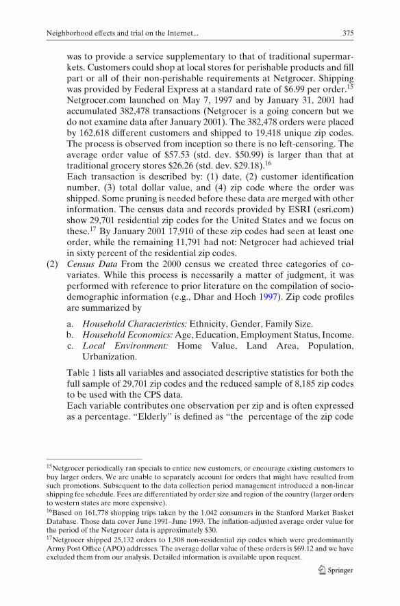
Table 1 lists all variables and associated descriptive statistics for both thefull sample of 29,701 zip codes and the reduced sample of 8,185 zip codesto be used with the CPS data.Each variable contributes one observation per zip and is often expressedas a percentage. “Elderly” is defined as “the percentage of the zip code
15Netgrocer periodically ran specials to entice new customers, or encourage existing customers tobuy larger orders. We are unable to separately account for orders that might have resulted fromsuch promotions. Subsequent to the data collection period management introduced a non-linearshipping fee schedule. Fees are differentiated by order size and region of the country (larger ordersto western states are more expensive).16Based on 161,778 shopping trips taken by the 1,042 consumers in the Stanford Market BasketDatabase. Those data cover June 1991–June 1993. The inflation-adjusted average order value forthe period of the Netgrocer data is approximately $30.17Netgrocer shipped 25,132 orders to 1,508 non-residential zip codes which were predominantlyArmy Post Office (APO) addresses. The average dollar value of these orders is $69.12 and we haveexcluded them from our analysis. Detailed information is available upon request.
376 D. R. Bell, S. Song
Tab
le1
Reg
ion
(zip
code
)ch
arac
teri
stic
san
dac
cess
tore
tail
serv
ices
Var
iabl
eD
escr
ipti
onF
ulld
ata
(n=
29,7
01)
CP
Ssu
bset
(n=
8,18
5)
Mea
nSt
dde
vM
ean
Std
dev
(1)
Hou
seho
ldch
arac
teri
stic
sB
lack
s%
ofB
lack
s0.
0725
0.15
630.
0880
0.16
65F
oreg
n%
offo
reig
nbo
rnin
divi
dual
s(a
ged
18+
)0.
0434
0.07
900.
0411
0.06
61H
ispa
nics
%of
His
pani
cs0.
0459
0.11
410.
0514
0.12
94L
arge
fam
ily%
offa
mili
esw
ith
five
orm
ore
mem
bers
0.15
150.
0607
0.14
730.
0589
Solo
fem
ale
%of
sing
lefe
mal
eho
useh
olds
0.04
770.
0245
0.04
810.
0277
Solo
mal
e%
ofsi
ngle
mal
eho
useh
olds
0.03
560.
0202
0.03
460.
0204
(2)
Hou
seho
ldec
onom
ics
Col
lege
%w
ith
bach
elor
san
d/or
grad
/pro
fdeg
ree
0.09
840.
0785
0.10
690.
0776
Eld
erly
%ag
ed65
and
abov
e0.
1371
0.05
860.
1268
0.06
16F
ullt
ime
fem
ale
%of
hous
ehol
dsw
ith
f-tf
emal
ew
orke
r0.
2545
0.08
390.
2799
0.07
80F
ullt
ime
mal
e%
ofho
useh
olds
wit
hf-
tmal
ew
orke
r0.
4850
0.11
970.
5033
0.11
20G
ener
atio
nX
%of
indi
vidu
als
25-3
4,in
com
es>
$50k
0.01
020.
0116
0.01
180.
0101
Wea
lthy
%of
hous
ehol
dsea
rnin
g$7
5k+
0.06
600.
0833
0.06
920.
0681

Neighborhood effects and trial on the Internet... 377
(3)
Loc
alen
viro
nmen
tD
ensi
tyP
opul
atio
nde
nsit
y1,
108.
0700
4,27
0.62
0099
9.73
801,
773.
7715
Hom
eva
lue
%of
hom
esva
lued
at$2
50k
orm
ore
0.02
320.
0782
0.01
540.
0477
Hou
seho
lds
Num
ber
ofho
useh
olds
3,09
5.40
004,
415.
5400
4,31
3.33
814,
526.
0870
Lan
dar
eaA
rea
insq
uare
mile
s11
0.21
2238
7.15
6760
.175
718
5.32
36L
arge
hous
e%
ofho
mes
wit
hfiv
ebe
droo
ms
orm
ore
0.03
390.
0324
0.02
790.
0264
Pop
ulat
ion
Tot
alpo
pula
tion
8,37
2.61
0011
,867
.600
011
,519
.016
011
,916
.306
0U
rban
hous
ing
%of
urba
nho
usin
gun
its
0.10
980.
1393
0.16
140.
1426
(4)
Acc
ess
tore
tail
serv
ices
Dis
tanc
eto
conv
enie
nce
Exp
ecte
dm
ax.d
ista
nce
toa
conv
enie
nce
stor
e6.
3172
8.02
023.
8641
4.82
40D
ista
nce
todr
ugE
xpec
ted
max
.dis
tanc
eto
adr
ugst
ore
7.82
078.
7894
5.33
705.
7469
Dis
tanc
eto
gene
ral
Exp
ecte
dm
ax.d
ista
nce
toa
gene
rals
tore
7.88
938.
4296
5.56
295.
6300
Dis
tanc
eto
supe
rmar
ket
Exp
ecte
dm
ax.d
ista
nce
toa
supe
rmar
ket
4.30
866.
0105
2.47
363.
2666
Dis
tanc
eto
war
ehou
seE
xpec
ted
max
.dis
tanc
eto
aw
areh
ouse
stor
e11
.066
59.
7632
8.76
856.
4391
(5)
Acc
ess
toin
tern
etB
road
band
acce
sspr
ovid
ers
No.
ofhi
gh-s
peed
ISP
s0.
3776
0.65
850.
5446
0.74
73C
PS
Inte
rnet
pene
trat
ion
MSA
mea
sure
from
CP
S0.
2474
0.14
22
378 D. R. Bell, S. Song
0
2000
4000
6000
8000
10000
12000
14000
16000
18000
20000
1 3 5 7 9 11 13 15 17 19 21 23 25 27 29 31 33 35 37 39 41 43 45
trial cumulative trial
0.000
0.010
0.020
0.030
0.040
0.050
0.060
0.070
1 3 5 7 9 11 13 15 17 19 21 23 25 27 29 31 33 35 37 39 41 43 45
hazard
a
b
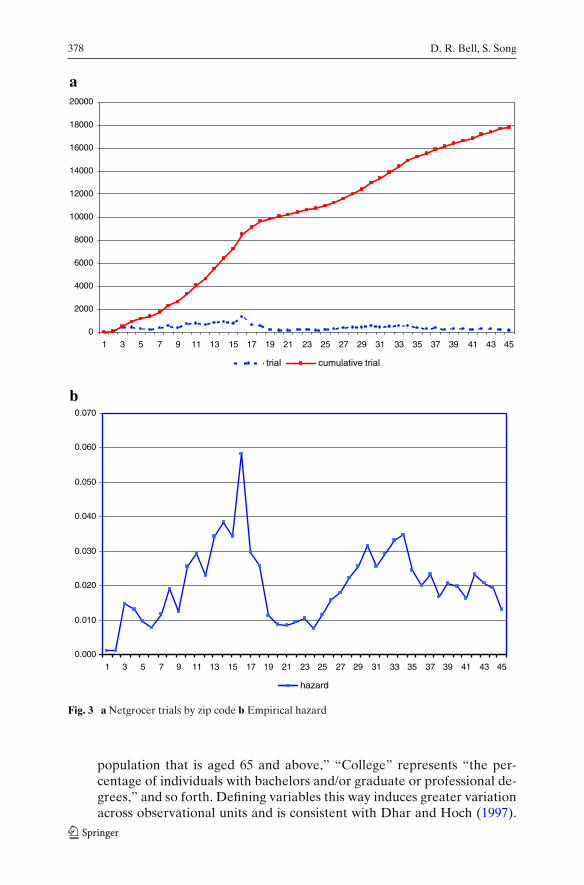
Fig. 3 a Netgrocer trials by zip code b Empirical hazard
population that is aged 65 and above,” “College” represents “the per-centage of individuals with bachelors and/or graduate or professional de-grees,” and so forth. Defining variables this way induces greater variationacross observational units and is consistent with Dhar and Hoch (1997).

Neighborhood effects and trial on the Internet... 379
a Trial as of December 1997
b Trial as of December 1998
c Trial as of December 1999
d Trial as of December 2000
Fig. 4 Space–time evolution of trial
This more “extreme” representation of the zip code characteristics (asopposed to using say average income, etc.) fits nicely with the idea thatthe first individual to try is a local innovator.
(3) Retail Competition Data. Nationwide distribution gives Netgrocer accessto a vast potential customer base and also exposes them to thousands ofcompetitors. As individuals in each zip code can still shop at local storesit is important to include information on the availability of this outsideor status quo option. CACI report the number of outlets and averagesales volume by zip code for five classes of retailer: convenience stores,drug stores, general merchandisers, supermarkets and warehouse clubs.We compute a measure of the maximum expected distance an individualwithin the zip code must travel to reach each type of store. Using zip
380 D. R. Bell, S. Song
Newark
New York
Brooklyn
No trial as of July 1997
Trial in May 1997
Trial in June 1997
Trial in July 1997
0 2.5 5 7.5 10
Miles
Newark
New York
Brooklyn
No trial as of Sep 1997
Trial before Aug 1997
Trial in Aug 1997
Trial in Sep 1997
0 2.5 5 7.5 10
Miles
Newark
New York
Brooklyn
No trial as of Nov 1997
Trial before Oct 1997
Trial in Oct 1997
Trial in Nov 1997
0 2.5 5 7.5 10
Miles
OaklandSan Francisco
No trial as of July 1997
Trial in May 1997
Trial in June 1997
Trial in July 1997
0 5 10 15 20
Miles
OaklandSan Francisco
No trial as of Sep 1997
Trial before Aug 1997
Trial in Aug 1997
Trial in Sep 1997
0 5 10 15 20
Miles
OaklandSan Francisco
No trial as of Nov 1997
Trial before Oct 1997
Trial in Oct 1997
Trial in Nov 1997
0 5 10 15 20
Miles
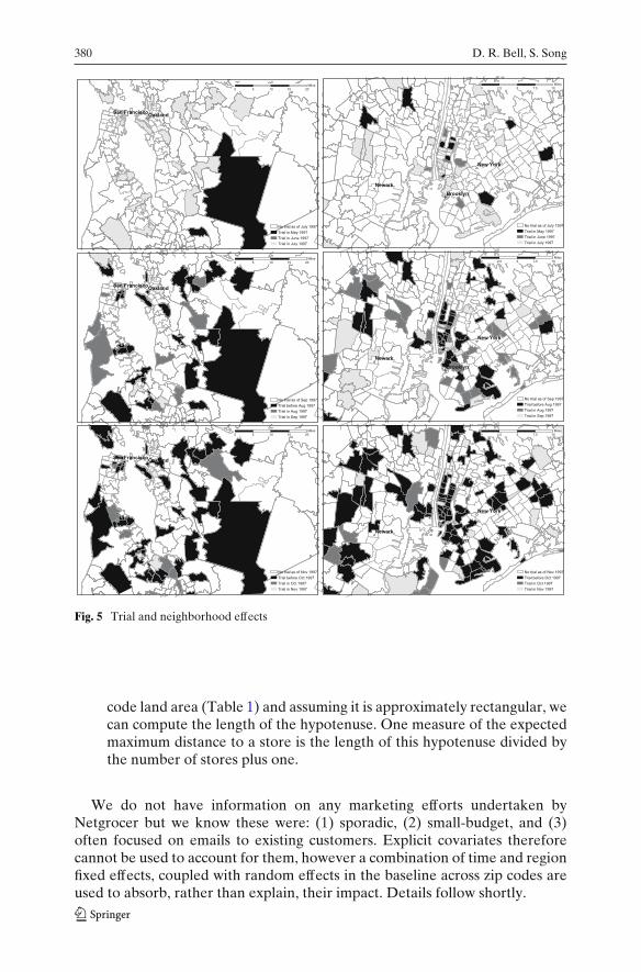
Fig. 5 Trial and neighborhood effects
code land area (Table 1) and assuming it is approximately rectangular, wecan compute the length of the hypotenuse. One measure of the expectedmaximum distance to a store is the length of this hypotenuse divided bythe number of stores plus one.
We do not have information on any marketing efforts undertaken byNetgrocer but we know these were: (1) sporadic, (2) small-budget, and (3)often focused on emails to existing customers. Explicit covariates thereforecannot be used to account for them, however a combination of time and regionfixed effects, coupled with random effects in the baseline across zip codes areused to absorb, rather than explain, their impact. Details follow shortly.
Neighborhood effects and trial on the Internet... 381
3.3 Preliminary analysis
Temporal Patterns The transaction data are organized into a matrix with29,701 rows (the number of zip codes) and 45 columns (the number ofmonths from May 1997 to January 2001). This gives 180,634 unique zip-monthcombinations where orders were observed. Figure 3a shows the number ofzip codes where trial occurred for the first time rose through August 1998and subsequently declined before rising again, and Fig. 3b plots the empiricalhazard (proportion of zip codes where trial occurred for the first time, amongthose where trial had not yet occurred at time t). The modeling implication isthat it will be important to control for time variation in the baseline hazard.
Spatial–Temporal Patterns By the end of May 1997 trial had occurred inthirty-four distinct zip codes ranging from New Jersey to California. Figure 4shows cumulative space-time trial patterns at one year intervals with the poolof triers expanding rapidly throughout the United States. These data revealthe most dramatic difference between a traditional retailer (where customersare contained within a relatively small area) and an e-tailer. More disaggregatevisual inspection of the patterns raises the possibility that neighborhood effectsplay a role. Trial at time t does not occur randomly in space. Rather, newtrials appear more likely to be located near contiguous neighborhoods whohave experienced trial prior to t. Figure 5 shows trial evolution in rolling 3-month increments for two separate east and west coast snapshots. As timemoves along new trials are more likely to arise close to contiguous areas ofprior trial.18
Neighbors A contiguous neighbor j is a zip code that shares an adjoiningboundary with the focal zip code z. Neighbor connectivity data was obtainedfor all 29,701 zip codes. The average number of regions in a neighborhood setis 5.63 (std. dev. = 2.28). Most zip codes have at least one neighbor, howeverthere are 136 “islands” who have no direct contiguous US neighbors.
4 Empirical findings
Special emphasis is given to demonstrating the neighborhood effect θ isproperly identified and robust to controls for heterogeneity, selection, andunobservables. The importance of measures of observed heterogeneity shouldnot however be overlooked. Our data set contains a far greater number ofcovariates than is typical in models of spatial effects. Bronnenberg and Mela(2004) for example, note the importance of random effects in their model toaccount for the influence of omitted variables such as market demographics.
18This visual pattern is representative of other months and regions. In the interests of brevity otherfigures are not shown but are available from the authors upon request.
382 D. R. Bell, S. Song
4.1 Estimation
The discrete time model with a complementary log-log specification mimics anunderlying continuous time process (see Appendix). We exploit the fact thatthe complementary log-log function is the inverse of the Gumbel cumulativedistribution function (see Allison 1982; Maritz and Munro 1967) used earlierto derive a regional level model from the individual behavior. Working fromthat derivation and substituting from equation (7)
log[−log(1−Pz(t))
] = log[−log
[exp {−exp(Vz(t) + ln(nz))}
]]= Vz(t) + ln(nz) (12)
The right hand side is therefore equivalent to the deterministic utility for thefirst trier from the region. Specifications for Vz(t) utilize covariates given inTable 1.
Recall yz(t) = 1 indicates the first trial occurred in zip code z at time t. Fornon-censored observations, let Tz reflect the time at which yz(t) = 1. It followsthat the number of observations zip z contributes for estimation is Tz with thedependent variable yz(s) equal to zero for all periods s with s < Tz. For the11,791 zip codes where trial is never observed and the data are censored, Tz =45 (May 1997 through January 2001, inclusive). The total number of stackedobservations in the full dataset is
∑z Tz = 910, 769. For the reduced dataset
created to examine Internet access using variables constructed from the CPS,there are 8,185 zip codes which generate 211,032 observations. In all instances,parameters are estimated via binary choice analysis with a complementary log-log link function on these stacked data.
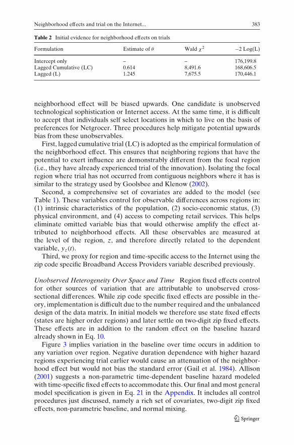
4.2 Initial evidence for neighborhood effects
In our first models the neighborhood effect and the population offset are thesole covariates. The neighborhood effect is formulated in two different ways
– As a lagged cumulative effect (LC) with elements of the column vectorfor neighbor behavior Yz(t − 1) containing the counts of all previous trialsoccurring up to and including time t − 1 in the neighbors of z, and
– As a standard lagged effect (L) with elements of Yz(t − 1) containing onlythe counts of trials that occurred at t − 1.
Contemporaneous representations violate the rationality conditions dis-cussed previously, and the associated parameters are not theoretically es-timable using maximum likelihood methods. Table 2 shows estimates for θ ,model fits and Wald χ2 statistics. θ is positive and significant for both formula-tions. The superior fit of the LC model occurs because it captures the influenceon focal region z of not only the first trial of a neighbor j, but also all trials thathave occurred in j between the initial trial at time s ≤ t − 1 and time t−1.
Unobserved Common Traits If contiguous regions share unobservedcommon traits that are positively correlated with the utility of trial, the
Neighborhood effects and trial on the Internet... 383
Table 2 Initial evidence for neighborhood effects on trials
Formulation Estimate of θ Wald χ2 −2 Log(L)
Intercept only – – 176,199.8Lagged Cumulative (LC) 0.614 8,491.6 168,606.5Lagged (L) 1.245 7,675.5 170,446.1
neighborhood effect will be biased upwards. One candidate is unobservedtechnological sophistication or Internet access. At the same time, it is difficultto accept that individuals self select locations in which to live on the basis ofpreferences for Netgrocer. Three procedures help mitigate potential upwardsbias from these unobservables.
First, lagged cumulative trial (LC) is adopted as the empirical formulation ofthe neighborhood effect. This ensures that neighboring regions that have thepotential to exert influence are demonstrably different from the focal region(i.e., they have already experienced trial of the innovation). Isolating the focalregion where trial has not occurred from contiguous neighbors where it has issimilar to the strategy used by Goolsbee and Klenow (2002).
Second, a comprehensive set of covariates are added to the model (seeTable 1). These variables control for observable differences across regions in:(1) intrinsic characteristics of the population, (2) socio-economic status, (3)physical environment, and (4) access to competing retail services. This helpseliminate omitted variable bias that would otherwise amplify the effect at-tributed to neighborhood effects. All these observables are measured atthe level of the region, z, and therefore directly related to the dependentvariable, yz(t).
Third, we proxy for region and time-specific access to the Internet using thezip code specific Broadband Access Providers variable described previously.
Unobserved Heterogeneity Over Space and Time Region fixed effects controlfor other sources of variation that are attributable to unobserved cross-sectional differences. While zip code specific fixed effects are possible in the-ory, implementation is difficult due to the number required and the unbalanceddesign of the data matrix. In initial models we therefore use state fixed effects(states are higher order regions) and later settle on two-digit zip fixed effects.These effects are in addition to the random effect on the baseline hazardalready shown in Eq. 10.
Figure 3 implies variation in the baseline over time occurs in addition toany variation over region. Negative duration dependence with higher hazardregions experiencing trial earlier would cause an attenuation of the neighbor-hood effect but would not bias the standard error (Gail et al. 1984). Allison(2001) suggests a non-parametric time-dependent baseline hazard modeledwith time-specific fixed effects to accommodate this. Our final and most generalmodel specification is given in Eq. 21 in the Appendix. It includes all controlprocedures just discussed, namely a rich set of covariates, two-digit zip fixedeffects, non-parametric baseline, and normal mixing.

384 D. R. Bell, S. Song
4.3 More evidence for neighborhood effects
Table 3 provides model fits and estimates for θ obtained after implementationof the control procedures outlined above. Rows 2 and 3 report the benchmarkfixed effects and non-parametric baseline hazard model fits. Where used theneighborhood effect (θ) enters according to the Lagged Cumulative (LC)specification. Rows 4 and 5 show that the effect is robust to the separateinclusion of two-digit zip fixed effects and a non-parametric baseline. Includingregion characteristics reduces the magnitude of θ and improves fit. The last rowshows θ for Model 10, the best fitting and most general model. It is still positiveand highly significant (θ = 0.170, Wald χ2 = 173.2). This model is especiallyinstructive as Internet access is proxied for and fixed effects are at the two-digitzip (rather than state) level.
Collectively, these results provide some assurance θ captures a behavioralprocess and does not simply mimic access to the Internet or unobserved
Table 3 More evidence for neighborhood effects on trials
Formulation Estimate of θ Wald χ2 −2 Log(L)
Benchmark models1. Intercept only – – 176,199.82. State fixed effects – – 159,266.53. Non-parametric baseline hazard – – 149,947.3
Models with neighborhood effect4. Lagged Cumulative (LC) θ
+ Two-digit zip code fixed effects 0.555 5,635.5 152,962.05. LC θ + Non-parametric baseline hazard 0.409 1,483.0 148,045.7
Models w/ neighborhood effect and covariates6. LC θ + Non-parametric baseline hazard
+ Region characteristics 0.272 484.9 144,359.97. LC θ + Non-parametric baseline hazard
+ Region characteristics+ Retail access 0.278 490.2 144,220.9
8. LC θ + Non-parametric baseline hazard+ Region characteristics+ Retail access+ Two-digit zip code fixed effects 0.144 159.3 142,682.0
9. LC θ + Non-parametric baseline hazard+ Region characteristics+ Retail access+ Two-digit zip code fixed effects+ Broadband access 0.131 127.7 142,638.8
10. LC θ + Non-parametric baseline hazard+ Region characteristics+ Retail access+ Two-digit zip code fixed effects+ Broadband access+ Random effect on intercept 0.170 173.2 142,510.0
Neighborhood effects and trial on the Internet... 385
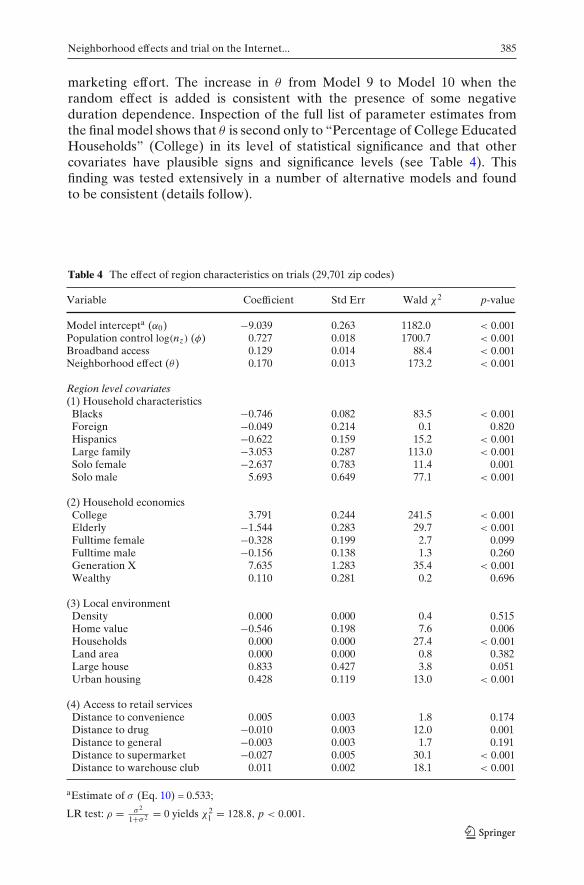
marketing effort. The increase in θ from Model 9 to Model 10 when therandom effect is added is consistent with the presence of some negativeduration dependence. Inspection of the full list of parameter estimates fromthe final model shows that θ is second only to “Percentage of College EducatedHouseholds” (College) in its level of statistical significance and that othercovariates have plausible signs and significance levels (see Table 4). Thisfinding was tested extensively in a number of alternative models and foundto be consistent (details follow).
Table 4 The effect of region characteristics on trials (29,701 zip codes)
Variable Coefficient Std Err Wald χ2 p-value
Model intercepta (α0) −9.039 0.263 1182.0 < 0.001Population control log(nz) (φ) 0.727 0.018 1700.7 < 0.001Broadband access 0.129 0.014 88.4 < 0.001Neighborhood effect (θ) 0.170 0.013 173.2 < 0.001
Region level covariates(1) Household characteristics
Blacks −0.746 0.082 83.5 < 0.001Foreign −0.049 0.214 0.1 0.820Hispanics −0.622 0.159 15.2 < 0.001Large family −3.053 0.287 113.0 < 0.001Solo female −2.637 0.783 11.4 0.001Solo male 5.693 0.649 77.1 < 0.001
(2) Household economicsCollege 3.791 0.244 241.5 < 0.001Elderly −1.544 0.283 29.7 < 0.001Fulltime female −0.328 0.199 2.7 0.099Fulltime male −0.156 0.138 1.3 0.260Generation X 7.635 1.283 35.4 < 0.001Wealthy 0.110 0.281 0.2 0.696
(3) Local environmentDensity 0.000 0.000 0.4 0.515Home value −0.546 0.198 7.6 0.006Households 0.000 0.000 27.4 < 0.001Land area 0.000 0.000 0.8 0.382Large house 0.833 0.427 3.8 0.051Urban housing 0.428 0.119 13.0 < 0.001
(4) Access to retail servicesDistance to convenience 0.005 0.003 1.8 0.174Distance to drug −0.010 0.003 12.0 0.001Distance to general −0.003 0.003 1.7 0.191Distance to supermarket −0.027 0.005 30.1 < 0.001Distance to warehouse club 0.011 0.002 18.1 < 0.001
aEstimate of σ (Eq. 10) = 0.533;
LR test: ρ = σ 2
1+σ 2 = 0 yields χ21 = 128.8, p < 0.001.
386 D. R. Bell, S. Song
4.4 Alternative models and specifications of the neighborhood effect
Several alternative models varied the definition of the risk set, restrictions onthe population offset, weights of the contiguity matrix (wz), and the elementsof the lagged neighborhood actions vector (Yz(t − 1)). These models wereestimated in order to examine the robustness of the basic neighborhood effectto different treatments (full results available upon request).
Formulations, Variables, Residuals A model with the constraint φ = 1 with arandom effect on the intercept and gives results essentially identical to thosein Table 3. Other specifications define nz as the number of households in theregion, not individuals. Again, the qualitative results are unchanged. A furthermodel uses cumulative adoptions at time t in addition to the neighborhoodeffect, and the effect remains. We tested the empirical veracity of the loga-rithmic form for population which follows from our derivation. A model withlinear through fourth order polynomial terms for population falls short on thebasis of fit, supporting our theory-driven choice. The Heckman–Singer (1984b)non-parametric approach to heterogeneity produced results essentially identi-cal to for our model with Normal mixing.
We checked for evidence of spatial autocorrelation in the residuals ofour final model, computing Moran’s I statistic using neighborhood contiguitymatrices as weights for all zip codes, for all 45 months. Ten months show signif-icant positive autocorrelation, two show significant negative autocorrelation,and the mean spatially-weighted residual is 0.005. The residuals are small inabsolute terms and decline in value with time (only two of the last 20 monthsshow significant positive values). As a point of comparison, we computed thesame test values for a model that is identical, but does not include θ . Here thepattern of autocorrelation is identical and the correlation between residuals formodels with and without θ is 0.98. Thus, we conclude that while some limitedevidence for spatial autocorrelation exists, it is clear that the neighborhoodeffect θ is not simply picking this up. As a final check, we re-estimated themodel but included neighborhood averages of all the demographic regressorsand Broadband access measure as covariates. In this case the qualitative resultswere unchanged and the point estimate of θ was 0.197 (Wald χ2 = 173.3); thenumber of instances of significant Moran’s I values declined from 12 to 9. Analternative approach would be to use non-parametric methods to obtain robuststandard errors (see Conley 1999; Conley and Molinari 2007).
Neighborhood Effect Covariate and Relationship to Other Studies We investi-gated alternative representations of the neighborhood effect through modifica-tions of wzYz(t − 1). Following the spirit of Bronnenberg and Mela (2004) whoconstructed wz using relative category volume at neighboring retailers we userelative population size: wz = POPz/
∑Nzj POP j. We also amended Yz(t − 1)
with the proportion of population trying, and simple binary indicators of thepresence or absence of prior trials. All such variations lead to θ values which

Neighborhood effects and trial on the Internet... 387
are positive and significantly different from zero, which again gives us someconfidence in the basic empirical finding.
Summary The pattern of results assessed through many alternative specifi-cations is consistent with the presence of neighborhood effects—every modelspecification produced qualitatively identical results. Our final model (Model10) employs a rich specification of observed heterogeneity, two-digit zip fixedeffects, a random effect on the baseline, and non-parametric time-dependence.In this model, as in all others, θ remains positive and significant, while the othercoefficients have plausible signs and levels of significance.
4.5 Substantive findings on the effect of region covariates on trial
Table 4 shows how region characteristics affect time to trial (a positivecoefficient means that the covariate speeds up the time to trial). Fourteenof twenty-three parameters are significantly different from zero (p < 0.01)and the implied marginal effects are intuitive. The magnitude and level ofsignificance of θ is unaffected by the presence of Broadband Access andthis variable itself is highly significant and correctly signed. Discussion of theremaining variables follows the classification in Table 1.
(1) Household Characteristics Regions with greater percentages of minoritiesexperience trial later, consistent with evidence for “digital divide” inwhich these groups have less access to the Internet and lower usage givenaccess (see for example, U.S. Department of Commerce annual studiesFalling Through the Net—Defining the Digital Divide). Percentage of soloperson households is also important, but interacts with gender: Regionswith greater proportions of male-only households see trial earlier. Con-versely, an increase in the proportion of large (greater than five person)households slows time to first trial. Larger families may prefer one stopshopping and Netgrocer does not sell perishables.
(2) Household Economics Higher percentages of tertiary-educated individ-uals leads to earlier trial. An increase in the number of young wealthyindividuals (Generation X) shows an additional positive effect, whereas ahigher percentage of elderly individuals slows time to trial. Other vari-ables held constant, working status household members shows no effect.
(3) Local environment The number of households, size of the housing unitand the extent of urbanization have a positive effect on the time to firsttrial. The latter two effects are weak (population is already controlledfor), but the collective impact is likely a proxy for the potential for socialinteraction within a region, and within and between household members.
(4) Access to Retail Services Estimates for convenience stores and generalmerchandisers suggest travel distance to either has no effect on Netgrocertrial. An increase in expected travel distance to drug stores and super-markets decreases time to first trial. While this may seen counterintuitive,it can be reconciled in light of the format differences. Netgrocer offers
388 D. R. Bell, S. Song
neither perishable products nor a full complement of drug store items.A household using Netgrocer would still need to visit a supermarket ordrug store. If the supermarket (for example) is relatively far away, then arational household might amortize the fixed cost of a trip by doing do one-stop shopping, thus eliminating any need to purchase non-perishables atNetgrocer. A household with better access to traditional stores might bemore willing to split the shopping basket for perishables (supermarket)and non-perishables (Internet). Conversely, Netgrocer seems to competemore directly with warehouse clubs. The less convenient the warehouseclub, the more likely shoppers are to try Netgrocer.
4.6 Internet access, censoring, and time variation in θ
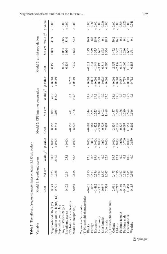
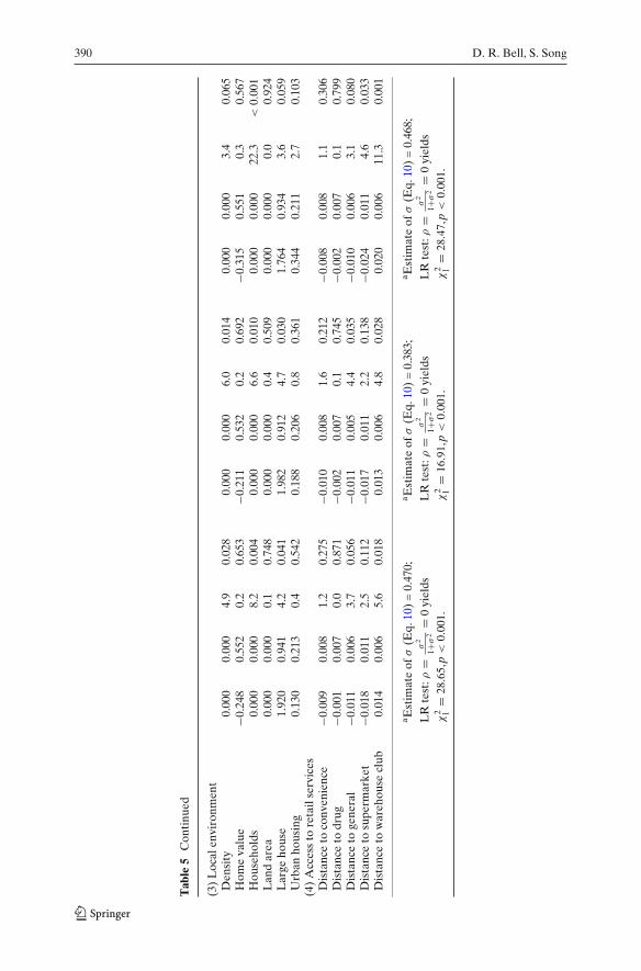
Our substantive conclusions have been based on a model that assumes: (1) thevariable Broadband Access Providers is a suitable proxy for Internet access,(2) all 29,701 zip codes can be used in estimation (i.e., this is a reasonabledefinition of the risk set), and (3) θ is a constant, conditional on the othercovariates. We provide results that suggest not only are these assumptionsempirically reasonable, but also that departure from them does not lead theneighborhood effect to break down or disappear. Table 5 provides estimatesfrom three different approaches to proxying for Internet access discussedearlier. Note that all three models use only the 8,185 zip codes in the reduceddataset because the CPS Internet penetration variables do not cover the entireUS. One other argument in favor of using the reduced MSA-level dataset is thefollowing. It is difficult to construct a good measure of ”proximity with regardto social contacts” across regions that vary greatly in terms of populationdensity; hence, the MSA-only sample which uses primarily high density zipcodes may constitute a superior sample.
Model 1 shows that the Broadband Access Providers covariate and theneighborhood effect are still positive and significant in the reduced dataset.Model 2 shows that while the neighborhood effect remains significant whenInternet access is proxied for with the CPS Internet Penetration variablederived from the CPS, the variable itself is not significant. Model 3 suggeststhat there is perhaps a better way to use the CPS data. Here, CPS InternetPenetration (CPSPenet) is interacted with the zip code population to in effectadjust the region-specific “risk set” to only those who are estimated as havingInternet access.19 The Broadband Access Providers variable is still included asa control (given the results from Model 1 in Table 5). Again, the neighborhoodeffect remains significant.
One could also look for evidence of spillover or neighborhood effects inzip codes that have no high speed access. A neighborhood effect estimate
19We control for over time variation in zip code level access to the Internet; one could also usesuch data to model changes in the “at risk” population. While only relatively crude controls forthe size of the risk set are available, the substantive results from a variety of formulations producequalitatively identical results.
Neighborhood effects and trial on the Internet... 389
Tab
le5
The
effe
ctof
regi
onch
arac
teri
stic
son
tria
ls(8
,185
zip
code
s)
Var
iabl
eM
odel
1:br
oadb
and
acce
ssM
odel
2:C
PS
inte
rnet
pene
trat
ion
Mod
el3:
at-r
isk
popu
lati
on
Coe
fSt
der
rW
ald
χ2
p-va
lue
Coe
fSt
der
rW
ald
χ2
p-va
lue
Coe
fSt
der
rW
ald
χ2
p-va
lue
Nei
ghbo
rhoo
def
fect
(θ)
0.14
30.
023
38.2
<0.
001
0.15
20.
022
45.9
<0.
001
0.15
00.
023
41.9
<0.
001
Pop
ulat
ion
cont
roll
og(n
z)
(φ)
0.72
10.
036
391.
7<
0.00
10.
744
0.03
544
3.9
<0.
001
Pop
ulat
ion
cont
roll
og(n
z∗C
PS
pene
t)(φ
′ )0.
627
0.03
336
8.5
<0.
001
Bro
adba
ndac
cess
0.12
20.
024
25.1
<0.
001
0.13
60.
024
31.0
<0.
001
CP
SIn
tern
etpe
netr
atio
n−0
.155
0.41
10.
10.
707
Mod
elin
terc
epta
(α0)
−8.6
560.
688
158.
3<
0.00
1−8
.626
0.70
614
9.3
<0.
001
−7.7
390.
673
132.
2<
0.00
1
Reg
ion
leve
lcov
aria
tes
(1)
Hou
seho
ldch
arac
teri
stic
sB
lack
s−0
.631
0.15
017
.8<
0.00
1−0
.601
0.14
417
.4<
0.00
1−0
.611
0.14
916
.8<
0.00
1F
orei
gn1.
642
0.55
38.
80.
003
1.58
10.
535
8.7
0.00
31.
631
0.54
98.
80.
003
His
pani
cs−1
.482
0.33
619
.4<
0.00
1−1
.422
0.32
519
.1<
0.00
1−1
.444
0.33
518
.6<
0.00
1L
arge
fam
ily−3
.331
0.63
227
.8<
0.00
1−3
.284
0.61
228
.8<
0.00
1−3
.193
0.62
725
.9<
0.00
1So
lofe
mal
e−0
.647
1.53
70.
20.
674
−0.7
231.
492
0.2
0.62
8−0
.514
1.52
50.
10.
736
Solo
mal
e7.
324
1.54
722
.4<
0.00
17.
807
1.48
827
.5<
0.00
16.
595
1.53
418
.5<
0.00
1(2
)H
ouse
hold
econ
omic
sC
olle
ge2.
991
0.47
539
.7<
0.00
12.
839
0.45
738
.6<
0.00
12.
955
0.47
239
.2<
0.00
1E
lder
ly−2
.217
0.53
617
.1<
0.00
1−2
.139
0.51
917
.0<
0.00
1−2
.137
0.53
216
.1<
0.00
1F
ullt
ime
fem
ale
0.16
00.
397
0.2
0.68
80.
227
0.38
60.
30.
557
0.21
60.
394
0.3
0.58
4F
ullt
ime
mal
e−0
.109
0.28
80.
10.
706
−0.0
970.
280
0.1
0.72
9−0
.065
0.28
60.
10.
820
Gen
erat
ion
X11
.458
2.68
518
.2<
0.00
111
.551
2.59
419
.8<
0.00
111
.019
2.66
217
.1<
0.00
1W
ealt
hy0.
115
0.56
50.
00.
839
0.20
20.
546
0.1
0.71
20.
185
0.56
10.
10.
741
390 D. R. Bell, S. Song
Tab
le5
Con
tinu
ed
(3)
Loc
alen
viro
nmen
tD
ensi
ty0.
000
0.00
04.
90.
028
0.00
00.
000
6.0
0.01
40.
000
0.00
03.
40.
065
Hom
eva
lue
−0.2
480.
552
0.2
0.65
3−0
.211
0.53
20.
20.
692
−0.3
150.
551
0.3
0.56
7H
ouse
hold
s0.
000
0.00
08.
20.
004
0.00
00.
000
6.6
0.01
00.
000
0.00
022
.3<
0.00
1L
and
area
0.00
00.
000
0.1
0.74
80.
000
0.00
00.
40.
509
0.00
00.
000
0.0
0.92
4L
arge
hous
e1.
920
0.94
14.
20.
041
1.98
20.
912
4.7
0.03
01.
764
0.93
43.
60.
059
Urb
anho
usin
g0.
130
0.21
30.
40.
542
0.18
80.
206
0.8
0.36
10.
344
0.21
12.
70.
103
(4)
Acc
ess
tore
tail
serv
ices
Dis
tanc
eto
conv
enie
nce
−0.0
090.
008
1.2
0.27
5−0
.010
0.00
81.
60.
212
−0.0
080.
008
1.1
0.30
6D
ista
nce
todr
ug−0
.001
0.00
70.
00.
871
−0.0
020.
007
0.1
0.74
5−0
.002
0.00
70.
10.
799
Dis
tanc
eto
gene
ral
−0.0
110.
006
3.7
0.05
6−0
.011
0.00
54.
40.
035
−0.0
100.
006
3.1
0.08
0D
ista
nce
tosu
perm
arke
t−0
.018
0.01
12.
50.
112
−0.0
170.
011
2.2
0.13
8−0
.024
0.01
14.
60.
033
Dis
tanc
eto
war
ehou
secl
ub0.
014
0.00
65.
60.
018
0.01
30.
006
4.8
0.02
80.
020
0.00
611
.30.
001
a Est
imat
eof
σ(E
q.10
)=
0.47
0;a E
stim
ate
ofσ
(Eq.
10)
=0.
383;
a Est
imat
eof
σ(E
q.10
)=
0.46
8;L
Rte
st:ρ
=σ
2
1+σ
2=
0yi
elds
LR
test
:ρ=
σ2
1+σ
2=
0yi
elds
LR
test
:ρ=
σ2
1+σ
2=
0yi
elds
χ2 1
=28
.65,
p<
0.00
1.χ
2 1=
16.9
1,p
<0.
001.
χ2 1
=28
.47,
p<
0.00
1.
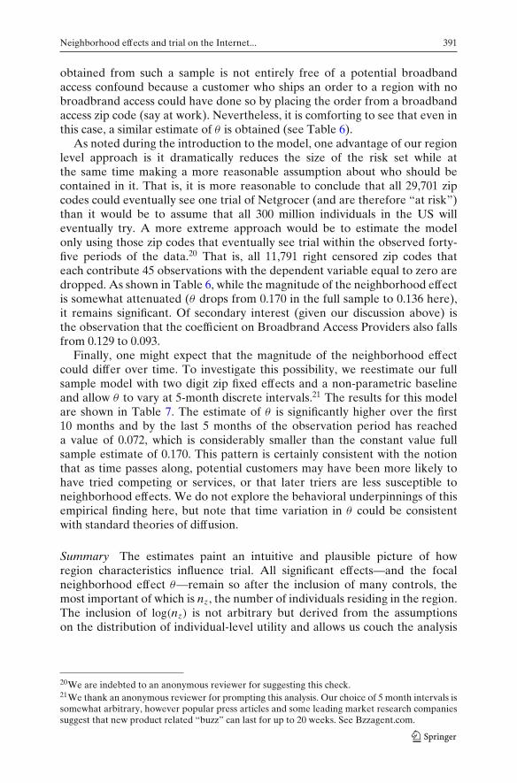
Neighborhood effects and trial on the Internet... 391
obtained from such a sample is not entirely free of a potential broadbandaccess confound because a customer who ships an order to a region with nobroadbrand access could have done so by placing the order from a broadbandaccess zip code (say at work). Nevertheless, it is comforting to see that even inthis case, a similar estimate of θ is obtained (see Table 6).
As noted during the introduction to the model, one advantage of our regionlevel approach is it dramatically reduces the size of the risk set while atthe same time making a more reasonable assumption about who should becontained in it. That is, it is more reasonable to conclude that all 29,701 zipcodes could eventually see one trial of Netgrocer (and are therefore “at risk”)than it would be to assume that all 300 million individuals in the US willeventually try. A more extreme approach would be to estimate the modelonly using those zip codes that eventually see trial within the observed forty-five periods of the data.20 That is, all 11,791 right censored zip codes thateach contribute 45 observations with the dependent variable equal to zero aredropped. As shown in Table 6, while the magnitude of the neighborhood effectis somewhat attenuated (θ drops from 0.170 in the full sample to 0.136 here),it remains significant. Of secondary interest (given our discussion above) isthe observation that the coefficient on Broadbrand Access Providers also fallsfrom 0.129 to 0.093.
Finally, one might expect that the magnitude of the neighborhood effectcould differ over time. To investigate this possibility, we reestimate our fullsample model with two digit zip fixed effects and a non-parametric baselineand allow θ to vary at 5-month discrete intervals.21 The results for this modelare shown in Table 7. The estimate of θ is significantly higher over the first10 months and by the last 5 months of the observation period has reacheda value of 0.072, which is considerably smaller than the constant value fullsample estimate of 0.170. This pattern is certainly consistent with the notionthat as time passes along, potential customers may have been more likely tohave tried competing or services, or that later triers are less susceptible toneighborhood effects. We do not explore the behavioral underpinnings of thisempirical finding here, but note that time variation in θ could be consistentwith standard theories of diffusion.
Summary The estimates paint an intuitive and plausible picture of howregion characteristics influence trial. All significant effects—and the focalneighborhood effect θ—remain so after the inclusion of many controls, themost important of which is nz, the number of individuals residing in the region.The inclusion of log(nz) is not arbitrary but derived from the assumptionson the distribution of individual-level utility and allows us couch the analysis
20We are indebted to an anonymous reviewer for suggesting this check.21We thank an anonymous reviewer for prompting this analysis. Our choice of 5 month intervals issomewhat arbitrary, however popular press articles and some leading market research companiessuggest that new product related “buzz” can last for up to 20 weeks. See Bzzagent.com.

392 D. R. Bell, S. Song
Tab
le6
The
effe
ctof
regi
onch
arac
teri
stic
son
tria
ls(a
lter
nati
vem
odel
s)
Var
iabl
eZ
ipar
eas
wit
hno
broa
dban
dac
cess
Rig
ht-c
enso
red
zip
area
sdr
oppe
d
Coe
ffici
ent
Std
err
Wal
dχ
2p-
valu
eC
oeffi
cien
tSt
der
rW
ald
χ2
p-va
lue
Mod
elin
terc
epta
(α0)
−9.5
340.
513
345.
2<
0.00
15.
202
76.8
080.
00.
946
Pop
ulat
ion
cont
roll
og(n
z)
(φ)
0.83
40.
027
970.
9<
0.00
10.
272
0.02
116
5.3
<0.
001
Bro
adba
ndac
cess
−−
−−
0.09
30.
017
31.4
<0.
001
Nei
ghbo
rhoo
def
fect
(θ)
0.17
80.
023
58.1
<0.
001
0.13
60.
017
67.5
<0.
001
Reg
ion-
leve
lcov
aria
tes
(1)
Hou
seho
ldch
arac
teri
stic
sB
lack
s−0
.421
0.16
16.
80.
009
−0.6
240.
107
34.0
<0.
001
For
eign
0.84
80.
454
3.5
0.06
20.
453
0.27
12.
80.
095
His
pani
cs−0
.325
0.32
01.
00.
310
−0.8
450.
209
16.3
<0.
001
Lar
gefa
mily
−3.5
930.
455
62.4
<0.
001
−2.1
680.
376
33.2
<0.
001
Solo
fem
ale
−1.9
161.
521
1.6
0.20
8−2
.665
1.09
25.
90.
015
Solo
mal
e5.
557
1.57
512
.5<
0.00
15.
745
1.01
632
.0<
0.00
1
(2)
Hou
seho
ldec
onom
ics
Col
lege
4.03
60.
421
92.0
<0.
001
4.18
70.
319
171.
8<
0.00
1E
lder
ly−1
.806
0.49
513
.3<
0.00
1−2
.076
0.36
232
.9<
0.00
1F
ullt
ime
fem
ale
0.25
90.
317
0.7
0.41
5−1
.293
0.26
124
.5<
0.00
1F
ullt
ime
mal
e0.
335
0.20
82.
60.
108
−0.4
240.
181
5.5
0.01
9G
ener
atio
nX
5.26
22.
321
5.2
0.02
311
.872
1.67
450
.3<
0.00
1W
ealt
hy0.
650
0.51
41.
60.
206
−0.4
950.
354
1.9
0.16
3
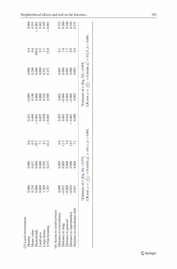
Neighborhood effects and trial on the Internet... 393
(3)
Loc
alen
viro
nmen
tD
ensi
ty0.
000
0.00
00.
60.
421
−0.0
000.
000
8.4
0.00
4H
ome
valu
e0.
210
0.41
10.
30.
609
0.14
80.
248
0.4
0.55
1H
ouse
hold
s0.
000
0.00
029
.7<
0.00
10.
000
0.00
038
8.0
<0.
001
Lan
dar
ea0.
000
0.00
07.
10.
007
0.00
00.
000
0.5
0.46
2L
arge
hous
e1.
209
0.58
34.
30.
038
0.55
40.
531
1.1
0.29
7U
rban
hous
ing
1.36
70.
213
41.2
<0.
001
0.58
60.
151
15.0
<0.
001
(4)
Acc
ess
tore
tail
serv
ices
Dis
tanc
eto
conv
enie
nce
0.00
00.
005
0.0
0.95
20.
002
0.00
50.
10.
713
Dis
tanc
eto
drug
−0.0
150.
005
11.5
0.00
1−0
.004
0.00
41.
00.
306
Dis
tanc
eto
gene
ral
−0.0
090.
004
5.8
0.01
6−0
.004
0.00
31.
70.
186
Dis
tanc
eto
supe
rmar
ket
−0.0
240.
006
14.5
<0.
001
−0.0
060.
006
0.9
0.34
2D
ista
nce
tow
areh
ouse
club
0.01
10.
004
7.1
0.00
80.
002
0.00
30.
40.
531
a Est
imat
eof
σ(E
q.10
)=
0.57
5;a E
stim
ate
ofσ
(Eq.
10)
=0.
954;
LR
test
:ρ=
σ2
1+σ
2=
0yi
elds
χ2 1
=16
1.1,
p<
0.00
1.L
Rte
st:ρ
=σ
2
1+σ
2=
0yi
elds
χ2 1
=41
2.5,
p<
0.00
1.

394 D. R. Bell, S. Song
Table 7 Time variation in θ
Variable Coefficient Std err Wald χ2 p-value
Model intercepta (α0) −8.767 0.282 968.5 < 0.001Population control log(nz) (φ) 0.693 0.020 1256.7 < 0.001Broadband access 0.078 0.013 37.5 < 0.001Neighborhood effect (θ) 0.408 0.083 24.2 < 0.001NE ∗ Month 6–10 −0.126 0.088 2.0 0.152NE ∗ Month 11–15 −0.271 0.084 10.4 0.001NE ∗ Month 16–20 −0.285 0.085 11.3 0.001NE ∗ Month 21–25 −0.328 0.089 13.7 < 0.001NE ∗ Month 26–30 −0.220 0.086 6.6 0.010NE ∗ Month 31–35 −0.277 0.086 10.4 0.001NE ∗ Month 36–40 −0.368 0.087 17.9 < 0.001NE ∗ Month 41–45 −0.326 0.088 13.8 < 0.001
Region level covariates(1) Household characteristics
Blacks −0.696 0.077 81.9 < 0.001Foreign −0.064 0.210 0.1 0.762Hispanics −0.588 0.144 16.7 < 0.001Large family −2.654 0.289 84.1 < 0.001Solo female −2.848 0.851 11.2 0.001Solo male 5.315 0.728 53.3 < 0.001
(2) Household economicsCollege 3.272 0.243 180.9 < 0.001Elderly −1.224 0.300 16.6 < 0.001Fulltime female −0.133 0.192 0.5 0.487Fulltime male −0.099 0.138 0.5 0.472Generation X 5.730 1.342 18.2 < 0.001Wealthy 0.101 0.272 0.1 0.712
(3) Local environmentDensity 0.000 0.000 0.3 0.604Home value −0.466 0.194 5.8 0.016Households 0.000 0.000 12.0 0.001Land area 0.000 0.000 1.1 0.294Large house 0.726 0.421 3.0 0.084Urban housing 0.331 0.111 8.9 0.003
(4) Access to retail servicesDistance to convenience 0.005 0.003 2.3 0.131Distance to drug −0.009 0.003 10.8 0.001Distance to general −0.002 0.002 1.1 0.296Distance to supermarket −0.026 0.006 22.8 < 0.001Distance to warehouse club 0.008 0.002 10.0 0.002
in terms of the first trial in each region, and to pool data across regions byimplicitly putting them on the same “scale.”
5 Discussion and conclusion
According to the 2007 Statistical Abstract compiled by the US Census Bureau,online retail sales were forecast at $95.3 billion for 2006, which represents
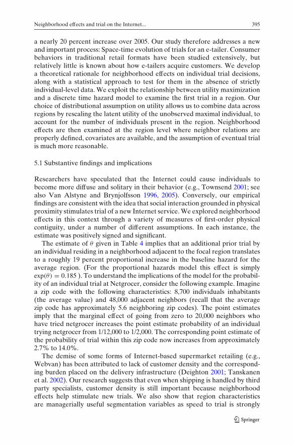
Neighborhood effects and trial on the Internet... 395
a nearly 20 percent increase over 2005. Our study therefore addresses a newand important process: Space-time evolution of trials for an e-tailer. Consumerbehaviors in traditional retail formats have been studied extensively, butrelatively little is known about how e-tailers acquire customers. We developa theoretical rationale for neighborhood effects on individual trial decisions,along with a statistical approach to test for them in the absence of strictlyindividual-level data. We exploit the relationship between utility maximizationand a discrete time hazard model to examine the first trial in a region. Ourchoice of distributional assumption on utility allows us to combine data acrossregions by rescaling the latent utility of the unobserved maximal individual, toaccount for the number of individuals present in the region. Neighborhoodeffects are then examined at the region level where neighbor relations areproperly defined, covariates are available, and the assumption of eventual trialis much more reasonable.
5.1 Substantive findings and implications
Researchers have speculated that the Internet could cause individuals tobecome more diffuse and solitary in their behavior (e.g., Townsend 2001; seealso Van Alstyne and Brynjolfsson 1996, 2005). Conversely, our empiricalfindings are consistent with the idea that social interaction grounded in physicalproximity stimulates trial of a new Internet service. We explored neighborhoodeffects in this context through a variety of measures of first-order physicalcontiguity, under a number of different assumptions. In each instance, theestimate was positively signed and significant.
The estimate of θ given in Table 4 implies that an additional prior trial byan individual residing in a neighborhood adjacent to the focal region translatesto a roughly 19 percent proportional increase in the baseline hazard for theaverage region. (For the proportional hazards model this effect is simplyexp(θ) = 0.185 ). To understand the implications of the model for the probabil-ity of an individual trial at Netgrocer, consider the following example. Imaginea zip code with the following characteristics: 8,700 individuals inhabitants(the average value) and 48,000 adjacent neighbors (recall that the averagezip code has approximately 5.6 neighboring zip codes). The point estimatesimply that the marginal effect of going from zero to 20,000 neighbors whohave tried netgrocer increases the point estimate probability of an individualtrying netgrocer from 1/12,000 to 1/2,000. The corresponding point estimate ofthe probability of trial within this zip code now increases from approximately2.7% to 14.0%.
The demise of some forms of Internet-based supermarket retailing (e.g.,Webvan) has been attributed to lack of customer density and the correspond-ing burden placed on the delivery infrastructure (Deighton 2001; Tanskanenet al. 2002). Our research suggests that even when shipping is handled by thirdparty specialists, customer density is still important because neighborhoodeffects help stimulate new trials. We also show that region characteristicsare managerially useful segmentation variables as speed to trial is strongly

396 D. R. Bell, S. Song
influenced by education levels, population density, extent of urbanization,access to retail services, and household composition.
5.2 Future research
We view this research as a first step and several issues remain. One could:
– Broaden the affiliation concept beyond that rooted in first-order geograph-ical contiguity. This could involve new variations on the retailer interactionmodels discussed in Bronnenberg and Mahajan (2001). Graff and Ashton(1993) find a reverse hierarchical process (from rural to urban areas) in thepattern of store openings by Walmart. Ter Hofstede et al. (2002) show thatcustomer similarities may reach across geographical boundaries. All theseapproaches could shed light on how e-tailers gain customers.
– Distinguish between effects that arise from direct word of mouth, ob-servational learning, and electronic communication. Godes and Mayzlin(2004) show the power of electronic word of mouth in predicting televisionviewing habits.
– Study purchase volumes. Chandrashearan and Sinha (1995) or repeatbehaviors (Urban 1975). A preliminary examination of our data showsthat initial orders for individuals who go on to repeat are approximatelyforty percent larger than those for individuals who try, but do not repeat.Moreover, the neighborhood effect disappears for the repeat decision.Individuals, having tried, appear to rely on their personal cost-benefitassessment in deciding to repeat.
We intend to visit these issues in future research.
Appendix
First, we show that the discrete time hazard with a complementary log-loglink function mirrors an underlying continuous time proportional hazardsmodel.22 Second, we show how to incorporate heterogeneity into the modelusing Normal mixing (estimates from this model are given in Table 4).
A Complementary log-log link function
Beginning with the continuous time hazard
λz(t) = limh→0
P(t < Tz ≤ t + �|Tz ≥ t)�
, (13)
we obtain the standard parameterized proportional hazards form
λz(t) = λ0(t) exp(xz(t)′β). (14)
22We are grateful to anonymous reviewers for providing references that led to this Appendix.

Neighborhood effects and trial on the Internet... 397
Here λ0(t) is the baseline hazard at time t, which is unknown, xz(t) is a vectorof time-dependent explanatory variables for region z, and β is a vector ofunknown parameters. The probability that a spell lasts until time t + 1 giventhat it has lasted until t is easily written as a function of the hazard
P(Tz ≥ t + 1|Tz ≥ t) = exp
[−
∫ t+1
tλz(u)du
]
= exp
[− exp(xz(t)′β) ·
∫ t+1
tλ0(u)du
](15)
given that xz(t) is constant between t and t + 1. Equation 15 can be written as
P(Tz ≥ t + 1|Tz ≥ t) = exp[− exp((xz(t)′β) + γ (t))
](16)
where
γ (t) = log
[∫ t+1
tλ0(u)du
]. (17)
This last expression shows that γ (t) is the logarithm of the integrated continu-ous time hazard. It then follows that the analog of Eq. 7 in the paper is simply
P(t ≤ Tz < t + 1|Tz ≥ t) = 1 − exp[− exp((xz(t)′β) + γ (t))
](18)
which is the claimed complementary log-log link function used for all modelsin the paper with time variation in the baseline hazard. The interested readeris referred to Seetharaman and Chintagunta (2001, equations 14 and 23)and Meyer (1990) for additional details. A second and final important pointabout this modeling choice concerns the distinction between the observationinterval—which we define exogenously as 1 month—and what one might calledthe consumer decision interval (which is unobserved by the analyst). Krishnanand Seetharaman (2002, see equations 8 and 9) provide a very nice result whichlinks the decision interval and the exogenous observation interval. They showthat the complementary log-log link function results as a limiting case whendecisions are made instantaneously. Absent other information, instantaneousdecision making at the zip code level is a reasonable approximation forInternet shopping behavior.
B Heterogeneity
While the discrete time model just shown incorporates time variation inthe baseline via γ (t), one may also wish to allow for heterogeneity overobservational units. In our case, we also need to allow for variation in thebaseline over regions z = 1, 2, . . . , Z . Our most general model accomplishesthis and the estimates are given in Table 4. Technical details for arriving at thisspecification are given below.
First, as noted in the paper, the data are organized into “sequential binaryresponse” form (Prentice and Gloeckler 1978; Han and Hausman 1990). Thepanel is arranged such that region z contributes Tz observations where 1 ≤
398 D. R. Bell, S. Song
Tz ≤ 45. Let t index observations for zip code z such that t = 1, 2, . . . , Tz. Weassume proportional hazards and introduce a positive-valued random variableor mixture ν
λz(t, νz) = λ0(t)νz exp(xz(t)′β)
= λ0(t) exp(xz(t)′β + uz), (19)
where λ0(t) is the baseline hazard, xz(t) is the same vector of observable covari-ates as above, and u ≡ log ν has density fu(u). The likelihood Lz(β, γ ) for eachregion with observed covariates xz(t) in this “mixed proportional hazards”model is
Lz(β, γ ) =∫ ∞
−∞
[Tz∏t=1
Pz(t, uz)yz(t)[1−Pz(t, uz)]1−yz(t)
]
× fu(uz)duz, (20)
where Pz(t, uz) = 1− exp(−exp(xz(t)′β+γ (t)+uz)) (21)
Because of the proportional hazards assumption, the covariates affect thehazard via the complementary log-log link. In estimation xz(t) also includesthe state or two-digit zip code fixed effects. As shown in the first section of thisAppendix, the γ (t) are interpreted as the log of a non-parametric piecewiselinear baseline hazard.
We model unobserved heterogeneity over z using Normal mixing. As notedearlier we also experimented with non-parametric mixing (Heckman andSinger 1984b), however the impact of the covariates and the shape of thebaseline hazard are very similar, but the fit slightly worse. Thus, results givenin Table 4 are based on Normal mixing.
Acknowledgements We thank seminar participants at Baruch College, Carnegie Mellon Uni-versity, Dartmouth College, HEC Paris, Humboldt University, Massachusetts Institute of Tech-nology, Singapore Management University, Stanford University, Tilburg University, University ofAuckland, UC San Diego, University of Houston, University of Michigan, University of SouthernCalifornia, University of Texas at Dallas and the 2004 Invitational Choice Symposium for insightsand comments, and Netgrocer CEO Lisa Kent for providing data and support. Detailed commentswere provided by Eric Bradlow, Peter Danaher, Steve Hoch, Ka Kok Lee, Phillip Leslie, GaryRussell, Seenu Srinivasan, Christophe Van den Bulte and John Zhang. Financial support for Songwas generously provided by WeBI, the Wharton School eBusiness Initiative and the MarketingScience Institute through the Alden G. Clayton Doctoral Dissertation Proposal Award. We arevery grateful to the Editor and two anonymous QME reviewers for several excellent suggestionsthat improved the paper. Any remaining errors are, of course, our own.
References
Allison, P. D. (1982). Discrete time methods for the analysis of event histories. In S. Leinhardt(Ed.), Sociological Methodology 1982 (pp. 61–98) . San Francsico, CA: Jossey-Bass.
Allison, P. D. (2001). Survival analysis using the SAS system: A practical guide. Cary, NC: SASInstitute.
Anselin, L. (1988). Spatial econometrics: Methods and models. Norwell, MA: Kluwer.

Neighborhood effects and trial on the Internet... 399
Besley, T., & Case, A. (1993). Modeling technology adoption in developing countries. AmericanEconomic Review 83(2), 396–402.
Bikhchandani, S., Hirshleifer, D., & Welch, I. (1998). Learning from the behavior of oth-ers: Conformity, fads and informational cascades. Journal of Economic Perspectives, 12(3),151–170.
Brock, W. A., & Durlaf, S. N. (2001). Discrete choice with social interactions. Review of EconomicStudies, 68, 235–260.
Bronnenberg, B., & Mahajan, V. (2001). Unobserved retailer behavior in multimarket data:Joint spatial dependence in market shares and promotion variables. Marketing Science, 20(3),284–299.
Bronnenberg, B. J., & Mela, C. F. (2004). Market roll-out and retailer adoption for new brands.Marketing Science, 23(4), 500–518.
Burt, R. S. (1980). Models of network structure. Annual Review of Sociology, 6, 79–141.Case, A. C. (1991). Spatial patterns in household demand. Econometrica, 59(4), 953–965.Case, A. C., Hines, J. R. Jr., & Rosen, H. S. (1989). Copycatting: Fiscal policies of states and their
neighbors. NBER Working Paper No. 3032.Case, A. C., Hines, J. R. Jr., & Rosen, H. S. (1993). Budget spillovers and fiscal policy interdepen-
dence: Evidence from the states. Journal of Public Economics, 52(3), 285–307.Chandrashekaran, M., & Sinha, R. K. (1995). Isolating the determinants of innovativeness: A split-
population tobit (SPOT) duration model of timing and volume of first and repeat purchase.Journal of Marketing Research, 32(3), 444–456.
Chaves, M. (1996). Ordaining women: The diffusion of an organizational innovation. AmericanJournal of Sociology, 101(4), 840–873.
Conley, T. G. (1999). GMM estimation with cross-sectional dependence. Journal of Econometrics,92, 1–45.
Conley, T. G., & Molinari, F. (2007). Spatial correlation robust inference with errors in location ordistance. Journal of Econometrics, doi:10.1016/j.jeconom.2006.09.003. (forthcoming)
Deighton, J. (2001). WebVan. Boston, MA: Harvard Business School Press.Dhar, S., & Hoch, S. J. (1997). Why store brand penetration varies by retailer. Marketing Science,
16(3), 208–227.Foster, A. D., & Rosenweig, M. R. (1995). Learning by doing and learning from others: Hu-
man capital and technological change in agriculture. Journal of Political Economy, 103(6),1176–1209.
Fotheringham, S. A. (1988). Consumer store choice and choice set definition. Marketing Science,7(3), 299–310.
Gail, M. H., Weiand, S., & Piantadosi, S. (1984). Biased estimates of treatment effects in ran-domized experiments with non-linear regressions and omitted covariates. Biometrika, 71(3),431–444.
Garber, T., Goldenberg, J., Libai, B., & Muller, E. (2004). From density to destiny: Using spatialdimension of sales data for early prediction of new product success. Marketing Science, 23(4),419–428.
Godes, D., & Mayzlin, D. (2004). Using online conversations to study word of mouth communica-tion. Marketing Science, 23(4), 530–534.
Goolsbee, A., & Klenow, P. J. (2002). Evidence on learning and network externalities in thediffusion of home computers. Journal of Law and Economics, 45(2), 317–342.
Greve, H. R., Strang, D., & Tuma, N. B. (1995). Specification and estimation of heterogeneousdiffusion models. In P. V. Marsden (Ed.), Sociological methodology (pp. 377-420). Cambridge,MA: Blackwell.
Graff, T. O., Ashton D. (1993). Spatial diffusion of Wal-Mart: Contagious and reverse hierarchicalelements. Professional Geographer, 46(1), 19–29.
Han, A., & Hausman, J. A. (1990). Flexible parametric estimation of duration and competing riskmodels: Summary. Journal of Applied Econometrics, 5(1), 1–28.
Heckman, J., Singer, B. (1984a). Econometric duration analysis. Journal of Econometrics, 24(1,2)63–132.
Heckman, J., Singer, B. (1984b). A method for minimizing the impact of distributional assumptionsin econometric models for duration data. Econometrica, 52, 271–318.
Howard, J. A., & Sheth, J. N. (1969). The theory of buyer behavior. New York, NY: Wiley.Huff, D. (1964). Redefining and estimating a trading area. Journal of Marketing, 28(3), 34–38.

400 D. R. Bell, S. Song
Krishnan, T. V. & Seetharaman, P. B. (2002). A flexible class of purchase incidence models.Review of Marketing Science, 1(3), Working paper 4.
Lilien, G. L., Kotler, P., & Moorthy, S. (1993). Marketing models. Englewood Cliffs, NJ: PrenticeHall.
Manski, C. F. (1993). Identification of endogenous social effects: The reflection problem. Reviewof Economic Studies, 60(3), 531–542.
Maritz, J. S., & Munro, A. H. (1967). On the use of the generalised extreme-value distribution inestimating extreme percentiles. Biometrics, 23(1), 79–103.
Meyer, B. D. (1990). Unemployment insurance and unemployment spells. Econometrica, 58,757–782.
Oyen, O., & De Fleur, M. L. (1953). The spatial diffusion of an airborne leaflet message. AmericanJournal of Sociology, 59(2), 144–149.
Prentice, R., & Gloeckler, L. (1978). Regression analysis of grouped survival data with applicationto breast cancer data. Biometrics, 34(1), 57–67.
Ryu, K. (1994). Group duration analysis of the proportional hazard model: Minimum chi-squaredestimators and specification tests. Journal of the American Statistical Association, 89(428),1386–1397.
Ryu, K. (1995). Analysis of a continuous-time proportional hazard model using discrete durationdata. Econometric Reviews, 14(3), 299–313.
Seetharaman, P. B. & Chintagunta, P. K. (2003). The proportional hazard model for pur-chase timing: A comparison of alternative specifications. Journal of Business and EconomicStatistics, 21(3), 368–382.
Singer, B., & Spilerman, S. (1983). The representation of social processes by Markov models.American Journal of Sociology, 82(1), 1–54.
Strang, D., & Tuma, N. B. (1993). Spatial and temporal heterogeneity in diffusion. AmericanJournal of Sociology, 99(3), 614–639.
Ter Hofstede, F., & Wedel, M. (1999). Time aggregation effects on the baseline of continuous-timeand discrete-time hazard models. Economics Letters, 63(5), 145–150.
Ter Hofstede, F., Wedel, M., & Steenkamp, J.-B. E. M. (2002). Identifying spatial segments ininternational markets. Marketing Science, 21(2), 160–177.
Tanskanen, K., Yrjola, H., & Holstrom, J. (2002). The way to profitable Internet groceryretailing—six lessons learned. International Journal of Retail and Distribution Management,30(4), 169–178.
Tolnay, S. E., Deane, G., & Beck, E. M. (1996). Vicarious violence: Spatial effects on southernlynchings, 1890-1919. American Journal of Sociology, 102(3), 788–815.
Townsend, A. M. (2001). Network cities and the global structure of the Internet. The AmericanBehavioral Scientist, 44(10), 1697–1716.
Urban, G. L. (1975). Perceptor—A model for product positioning. Management Science, 21(8),858–870.
Van den Bulte, C., & Lilien, G. L. (2001). Medical Innovation revisited: Social contagion versusmarketing effort. American Journal of Sociology, 106(5), 1409–1453.
Van Alstyne, M., & Brynjolfsson, E. (1996). Could the Internet balkanize science? Science,274(5292), 1479–1480.
Van Alstyne, M., & Brynjolfsson, E. (2005). Global village or cyber-balkans? Modeling andmeasuring the integration of electronic communities. Management Science, 51(6), 851–868.
Yang, S., & Allenby, G. M. (2003). Modeling interdependent consumer preferences. Journal ofMarketing Research 40(3), 282–294.