1

Nervous System Stimulation Using

Microwave

By Md Anas Boksh Mazady

Project report of ELCT 891B

This article is intended to investigate the possibilities of using microwave to stimulate the

human nervous system so that people with peripheral nervous system disorders could be

cured with non-invasive technique. We will start with first describing the human nervous

system, and then we will try having some insight of how the signal propagates through

this system. Later in this report we will review two papers, one of which will be dealing

with the modeling of the stimulation of a nerve fiber, and the other will be dealing with

the considerations to design a magnetic coil to serve as a stimulator. I will finish this

article by describing my own findings in designing a magnetic coil.

1. HUMAN NERVOUS SYSTEM

The human nervous system can broadly be categorized into two components, namely- the

central nervous system and the peripheral nervous system. Brain, spinal cord, and nerve

roots constitute the central nervous system. On the other hand, thirty one pairs of nerve

roots when branches off the spinal cord to enable the body to move and feel are called the

peripheral nerves.

As shown in figure 1, spinal cord is extended from the lower part of the brain through the

lower part of the body. It is responsible for carrying signal to and from the brain and

different organs. Information about movement of our different limbs and organs or the

information about how we feel in different environments, all of these communications

between the body and brain are conveyed by the cable like structure of the spinal cord.

This spinal cord is about an inch in diameter and 18 inches in length at its widest point.

The peripheral nerves can be categorized into five sub-sections according to their

function in human body.

1) Cervical Nerves (8 pairs of nerves)

2) Thoracic Nerves (12 pairs of nerves)

3) Lumbar Nerves (5 pairs of nerves)

4) Sacral Nerves (5 pairs of nerves)

5) Coccyx Nerves (1 pair of nerve)

2

Figure 1: Human nervous system structure

Cervical nerves are responsible for the proper functioning of head, neck, breathing, upper

arms, wrists, hands etc. Thoracic nerves, on the other hand, are responsible for the

functioning of chest, abdominal muscle, internal organs etc. Similarly, lumbar nerves are

for leg muscles, sacral nerves for bathroom capabilities, and coccyx nerves for parental

capabilities

The spinal cord is protected by a hard shell called vertebrae.

Figure 2: Vertebrae

3

2. SIGNAL PROPAGATION IN HUMAN NERVOUS SYSTEM

Neuron is the unit particle of the nervous system. When a neuron receives a stimulus,

depending on the strength of the stimulus, it creates electrical pulses. These pulses then

propagate through its cable like structure.

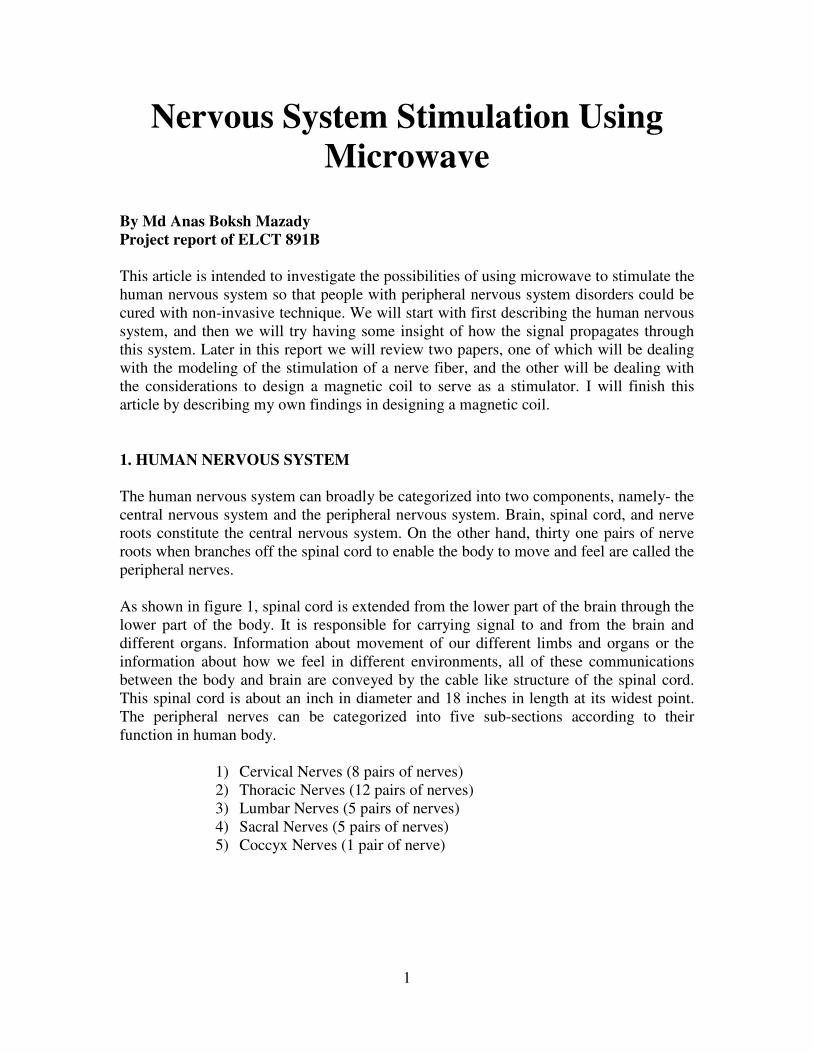
Figure 3: A neuron cell

The pulses always have constant magnitudes and duration irrespective of the strength of

the stimulus. The intensity of the stimulus is conveyed by the number of pulses produced.

The cell has input ends named dendrites and a long tail – axon. The axons differ in

lengths for different parts of the body. The longest axons might even be more than 1

meter in length. Some of these axons are covered with fatty materials called myelin.

These myelin sheaths are about 2 mm long, separated by gaps named Node of Ranvier.

Human axons are very narrow in diameter. The largest axon might have a diameter of 20

µm. Squid have comparatively thicker axons. This is the reason why most of the

experiments are done on squid axons.

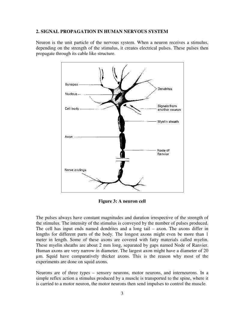
Neurons are of three types – sensory neurons, motor neurons, and interneurons. In a

simple reflex action a stimulus produced by a muscle is transported to the spine, where it

is carried to a motor neuron, the motor neurons then send impulses to control the muscle.

4

Figure 4: Reflex action

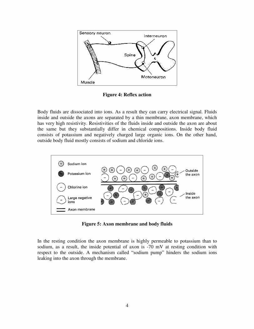
Body fluids are dissociated into ions. As a result they can carry electrical signal. Fluids

inside and outside the axons are separated by a thin membrane, axon membrane, which

has very high resistivity. Resistivities of the fluids inside and outside the axon are about

the same but they substantially differ in chemical compositions. Inside body fluid

consists of potassium and negatively charged large organic ions. On the other hand,

outside body fluid mostly consists of sodium and chloride ions.

Figure 5: Axon membrane and body fluids

In the resting condition the axon membrane is highly permeable to potassium than to

sodium, as a result, the inside potential of axon is -70 mV at resting condition with

respect to the outside. A mechanism called “sodium pump” hinders the sodium ions

leaking into the axon through the membrane.

5

2.1 Action Potential

If the stimulus exceeds a certain threshold, typically 15 mV higher than the resting value,

an impulse is then produced which propagates down the axon. This propagating impulse

is known as action potential.

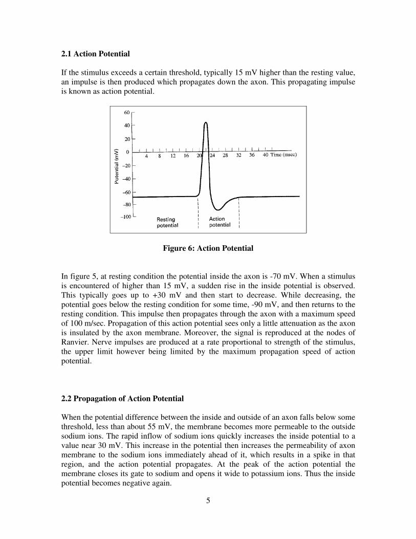
Figure 6: Action Potential

In figure 5, at resting condition the potential inside the axon is -70 mV. When a stimulus

is encountered of higher than 15 mV, a sudden rise in the inside potential is observed.

This typically goes up to +30 mV and then start to decrease. While decreasing, the

potential goes below the resting condition for some time, -90 mV, and then returns to the

resting condition. This impulse then propagates through the axon with a maximum speed

of 100 m/sec. Propagation of this action potential sees only a little attenuation as the axon

is insulated by the axon membrane. Moreover, the signal is reproduced at the nodes of

Ranvier. Nerve impulses are produced at a rate proportional to strength of the stimulus,

the upper limit however being limited by the maximum propagation speed of action

potential.

2.2 Propagation of Action Potential

When the potential difference between the inside and outside of an axon falls below some

threshold, less than about 55 mV, the membrane becomes more permeable to the outside

sodium ions. The rapid inflow of sodium ions quickly increases the inside potential to a

value near 30 mV. This increase in the potential then increases the permeability of axon

membrane to the sodium ions immediately ahead of it, which results in a spike in that

region, and the action potential propagates. At the peak of the action potential the

membrane closes its gate to sodium and opens it wide to potassium ions. Thus the inside

potential becomes negative again.

6

Figure 7: Propagation of action potential. (a) Membrane becoming permeable to

sodium, (b) Membrane closing its gate to sodium and opening to potassium making

the inside potential negative again.

Although the signal propagates by the transportation of the ions, the net flow of ions is

much lower than number of ions at rest. Let’s illustrate with some calculations.

We know,

∆Q = C ∆V

But the potential difference inside the axon, ∆V = 70 mV - (-30) mV = 100 mV

And the capacitance per unit length of a non-myelinated axon is C = 7103 −× F/m (see

table 1)

So the difference in charge appears to be ∆Q = 8103 −× C. Which gives the indication

that the number of sodium ions entering per meter of axon length is ∆Q/q = 1.875 1110× ,

this is much lower a number than the number of ions at rest ( 15107 × ).

7

During the propagation of the action potential, the above capacitance is continuously

discharged and recharged. The energy required to charge 1 m length of non-myelinated

axon can be calculated as

9272 105.1)1.0(1032

1

2

1 −− ×=×××== CVE J/m

Since, the duration of the pulse is different for different part of the body. In the muscle

fiber the duration is usually longer, about 20 msec whereas in heart muscle it may last a

quarter of a second. Let’s assume a duration of 1/100 sec for this case, then the power

required to charge the capacitor is 7105.1 −× W/m.

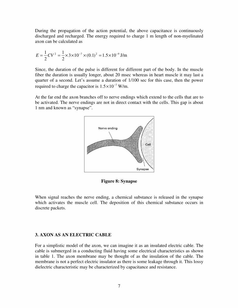
At the far end the axon branches off to nerve endings which extend to the cells that are to

be activated. The nerve endings are not in direct contact with the cells. This gap is about

1 nm and known as “synapse”.

Figure 8: Synapse

When signal reaches the nerve ending, a chemical substance is released in the synapse

which activates the muscle cell. The deposition of this chemical substance occurs in

discrete packets.

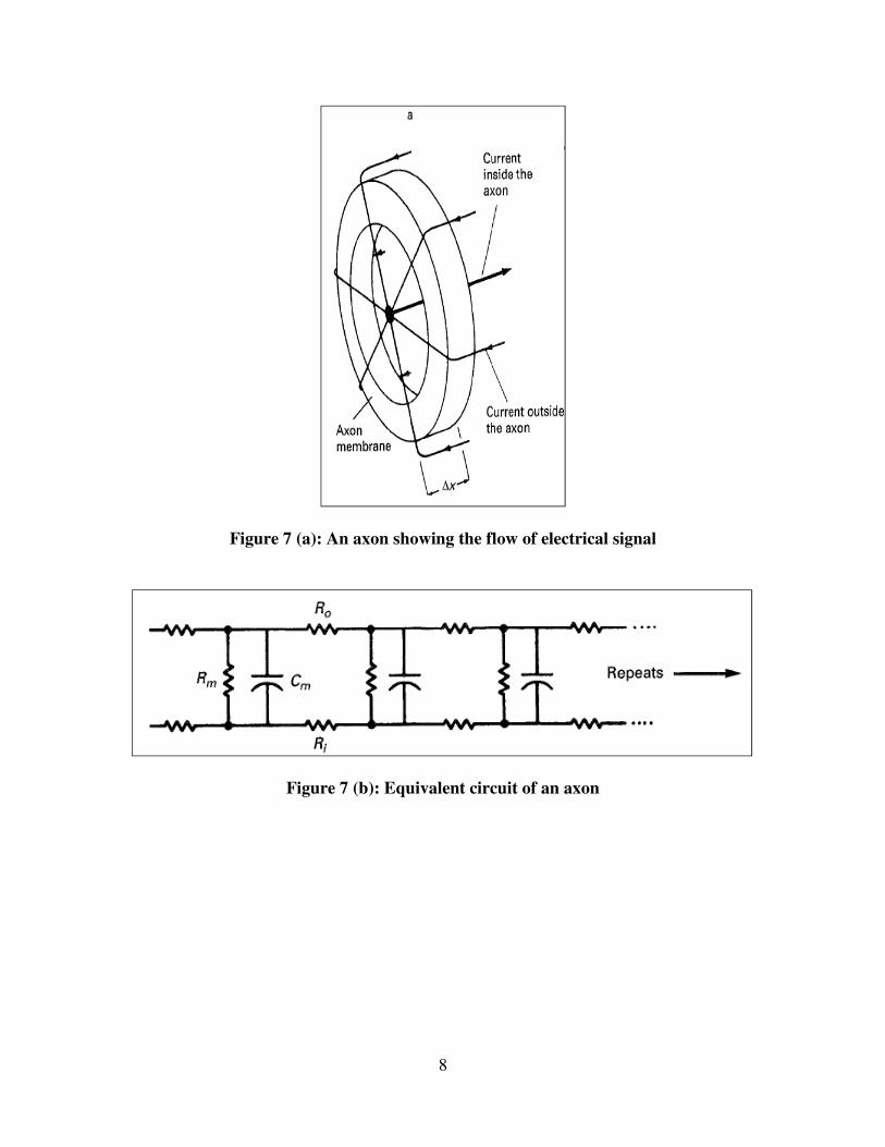
3. AXON AS AN ELECTRIC CABLE

For a simplistic model of the axon, we can imagine it as an insulated electric cable. The

cable is submerged in a conducting fluid having some electrical characteristics as shown

in table 1. The axon membrane may be thought of as the insulation of the cable. The

membrane is not a perfect electric insulator as there is some leakage through it. This lossy

dielectric characteristic may be characterized by capacitance and resistance.

8

Figure 7 (a): An axon showing the flow of electrical signal

Figure 7 (b): Equivalent circuit of an axon

9

Table 1: Electrical properties of an axon

However, this model has some limitations as it fails to explain some key characteristics

of an axon. First, in the above circuit electrical signal flows at a speed comparable to the

speed of light ( 8103× m/sec) but as we know the maximum speed of propagation of an

electrical signal through an axon is limited to 100 m/sec. Second, in the above circuit

electrical signals decay very quickly but in an axon action potentials propagate with very

low attenuation. These shortcomings of the above model will be accounted for in a

modified circuit model, Hodgkin-Huxley model, the description of which follows later in

this report.

4. DESIGN CONSIDERATIONS

Here we will review two papers which will give us some insight about the design

consideration of stimulation circuitry. The first paper describes an improved model of the

nerve fiber. The authors then research the location of maximum stimulation along the

nerve fiber. The second paper studies different magnetic coils to give an insight of which

configuration will be better suited for a particular application of nerve stimulation.

4.1.1 Model of a Nerve fiber

To continue from where we have stopped in Article 3, let’s review the paper by B. J.

Roth et al (Roth & Basser, June 1990).

10

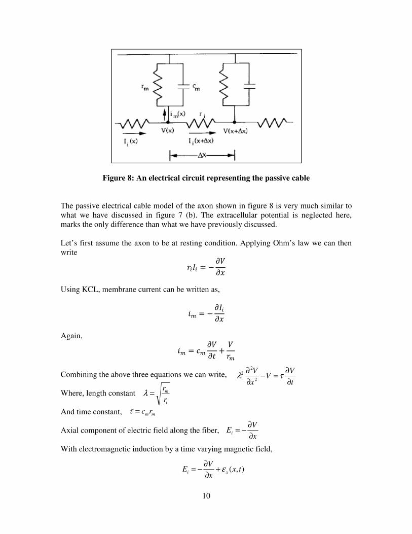
Figure 8: An electrical circuit representing the passive cable

The passive electrical cable model of the axon shown in figure 8 is very much similar to

what we have discussed in figure 7 (b). The extracellular potential is neglected here,

marks the only difference than what we have previously discussed.

Let’s first assume the axon to be at resting condition. Applying Ohm’s law we can then

write

= −

Using KCL, membrane current can be written as,

= −

Again,

= +

Combining the above three equations we can write,

Where, length constant

And time constant,

Axial component of electric field along the fiber,

With electromagnetic induction by a time varying magnetic field,

t

VV

x

V

∂

∂=−

∂

∂τλ

2

22

i

m

r

r=λ

mmrc=τ

x

VEi

∂

∂−=

),( txx

VE xi ε+

∂

∂−=

11

Where (, ) is the induced electric field parallel to the the axis of the axon.

But the induced electric field equals the negative rate of change of the vector magnetic

potential

Now, = − + (, )

So, ……………………. (1)

Let’s note that the derivative of the electric field, not the electric field itself, appears in

the equation. This is because the membrane current , not the axial current along the

fiber, depolarizes the axon.

The membrane current is a maximum when the spatial gradient of the axial component of

the current is maximum and the induced electric field is at its highest.

From equation (1) we can draw an interesting conclusion, stimulation is not maximum at

the locations where the induced electric field is maximum rather it would be zero there.

The locations where the gradient of the electric field is maximum will have maximum

stimulation.

This model suffers from the limitations that we have previously discussed in Article 3.

So, in the next article a modified approach has been discussed.

4.1.2 Hodgkin-Huxley Model

Figure 9: Hodgkin-Huxley model of nerve fiber

t

A

∂

∂−=

rrε

xt

VV

x

V x

∂

∂+

∂

∂=−

∂

∂ ελτλ 2

2

22

12

The Hodgkin-Huxley model of the nerve fiber takes care of the membrane permeability

to the sodium and potassium ions. The three conductances in each branch represent the

membrane leakage, the sodium channel, and the potassium channel. The value of this

parameters are summarized in table 2.

Table 2: Parameter values for Hodgkin-Huxley model

With this modification the cable equation becomes 2 − ℎ( − ) + !"( − ) + #( − #)$

= % + 2 (, )

Where, m, h, n can be found solving the below three differential equations,

And, &, ', &(, '(, &), ') can be calculated from the below four differential equations,

13

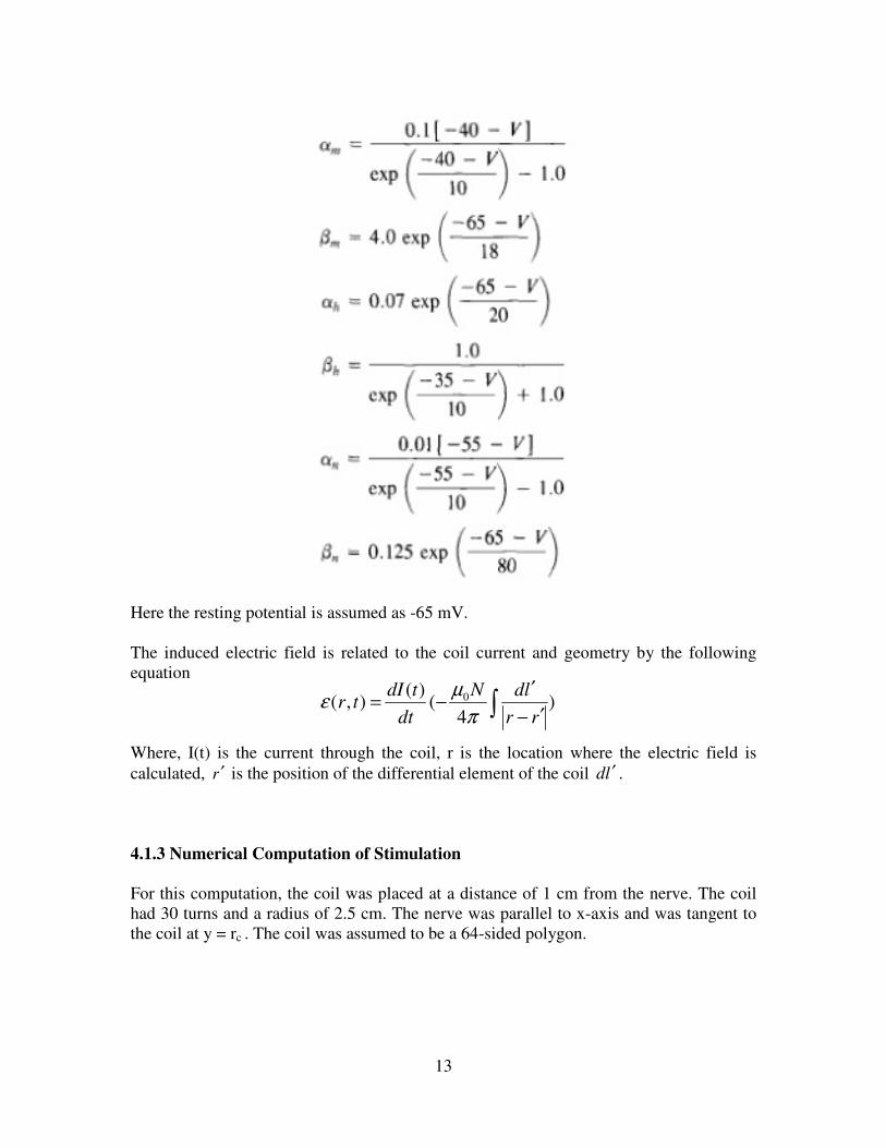
Here the resting potential is assumed as -65 mV.

The induced electric field is related to the coil current and geometry by the following

equation

Where, I(t) is the current through the coil, r is the location where the electric field is

calculated, r ′ is the position of the differential element of the coil ld ′ .

4.1.3 Numerical Computation of Stimulation

For this computation, the coil was placed at a distance of 1 cm from the nerve. The coil

had 30 turns and a radius of 2.5 cm. The nerve was parallel to x-axis and was tangent to

the coil at y = rc . The coil was assumed to be a 64-sided polygon.

∫ ′−

′−= )

4(

)(),( 0

rr

ldN

dt

tdItr

π

µε

14

Figure 10: Coil arrangement for stimulation

4.1.4 Electric Field and its gradient

Figure 11 (a): Electric field profile (*+*, = 1 ./01)

15

Figure 11 (a) shows the electric field profile for the arrangement of figure 10. The

corresponding electric field gradient is shown in figure 11 (b).

Figure 11 (b): Electric field gradient

It is interesting to note that the maximum of electric field gradient is not below the center

of the coil nor even at the edges.

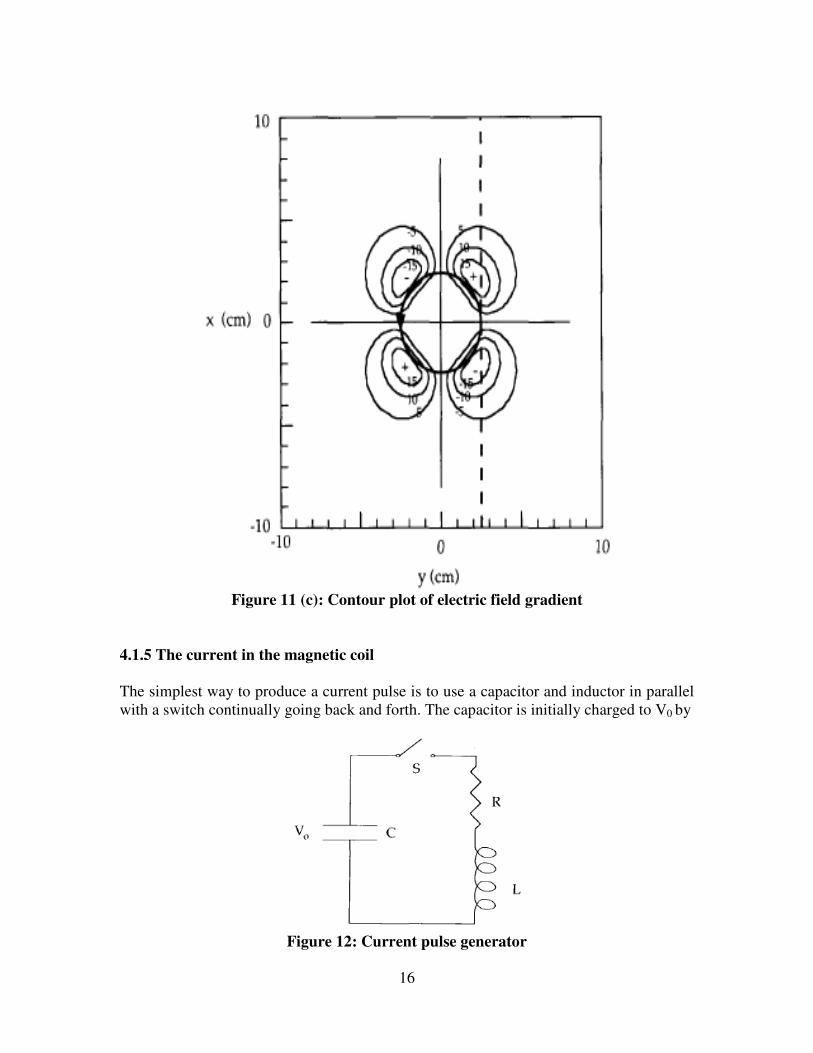
Figure 11 (c) shows the contour plot of the spatial profile of electric field gradient. The

bold circle represents the position of the magnetic coil with the arrow indicating the

direction of rate of change of current. The dotted line indicates the location of the axon.

The minus signs indicate the location of depolarization, i.e. stimulation, whereas the plus

signs indicate the location of hyper polarization.

16

Figure 11 (c): Contour plot of electric field gradient

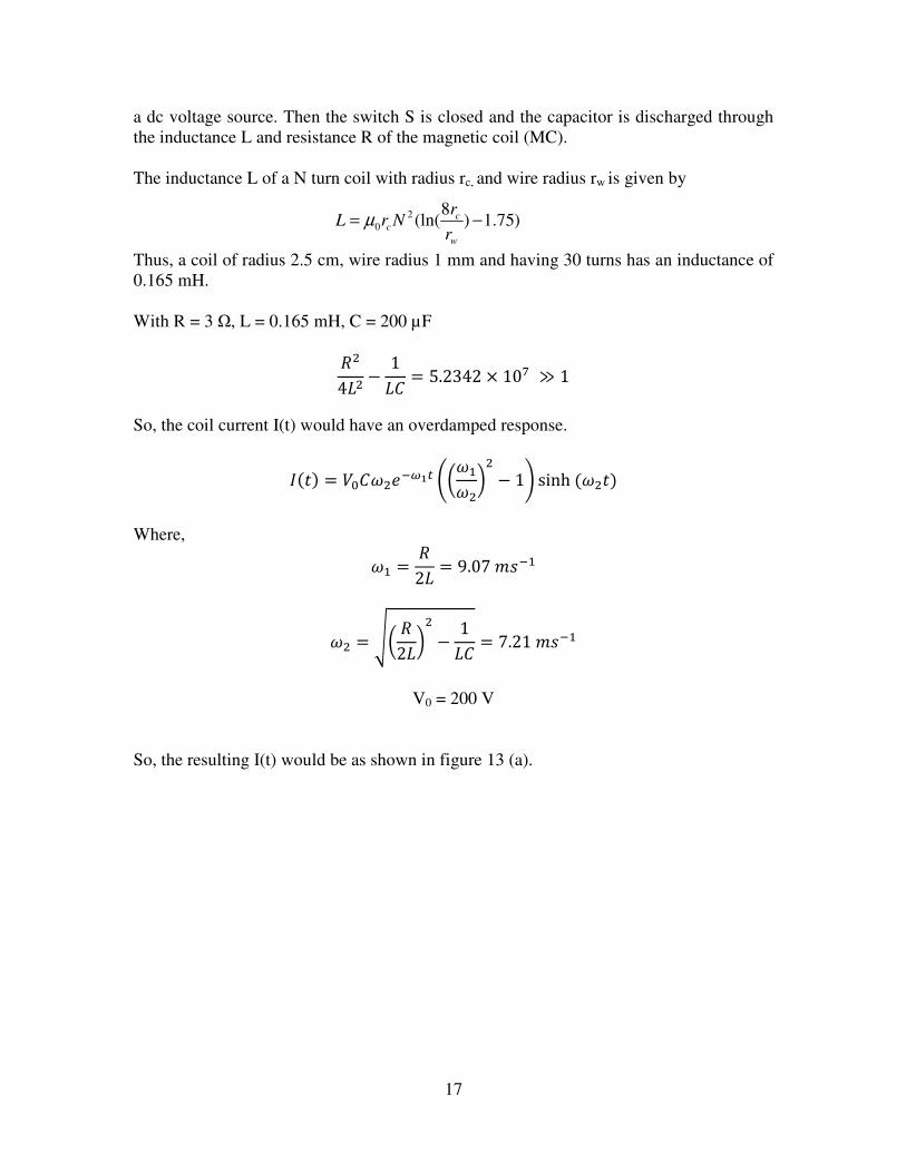
4.1.5 The current in the magnetic coil

The simplest way to produce a current pulse is to use a capacitor and inductor in parallel

with a switch continually going back and forth. The capacitor is initially charged to V0 by

Figure 12: Current pulse generator

17

a dc voltage source. Then the switch S is closed and the capacitor is discharged through

the inductance L and resistance R of the magnetic coil (MC).

The inductance L of a N turn coil with radius rc, and wire radius rw is given by

Thus, a coil of radius 2.5 cm, wire radius 1 mm and having 30 turns has an inductance of

0.165 mH.

With R = 3 Ω, L = 0.165 mH, C = 200 µF

43 − 13% = 5.2342 × 109 ≫ 1

So, the coil current I(t) would have an overdamped response.

() = ;%<=>?@A BC<D<E − 1F sinh (<)

Where,

<D = 23 = 9.07 1>D

< = MC 23E − 13% = 7.21 1>D

V0 = 200 V

So, the resulting I(t) would be as shown in figure 13 (a).

)75.1)8

(ln(2

0 −=w

cc

r

rNrL µ

18

Figure 13 (a): Current in a magnetic coil

The time derivative of I(t) would then be as shown in figure 13 (b).

Figure 13 (b): Time derivative of current in a magnetic coil (MC)

Taking this time derivative of current into consideration the electric field gradient in

figure 11 (b) will be modified to figure 14.

19

Figure 14: Electric field gradient taking MC current into consideration

4.1.6 Conclusion from (Roth & Basser, June 1990)

From this paper we can draw several important conclusions.

1. The nerve fiber is stimulated by the gradient of the electric field that is parallel to

the axis of the nerve fiber.

2. The electric field component hyperpolarizes or depolarizes the axon and may

invoke an action potential depending on the strength of the electric field.

3. Hodgkin-Huxley model was introduced to represent a nerve fiber.

4. Maximum stimulation is neither below the center of the coil nor below its edges.

4.2 Magnetic Coil Design Considerations

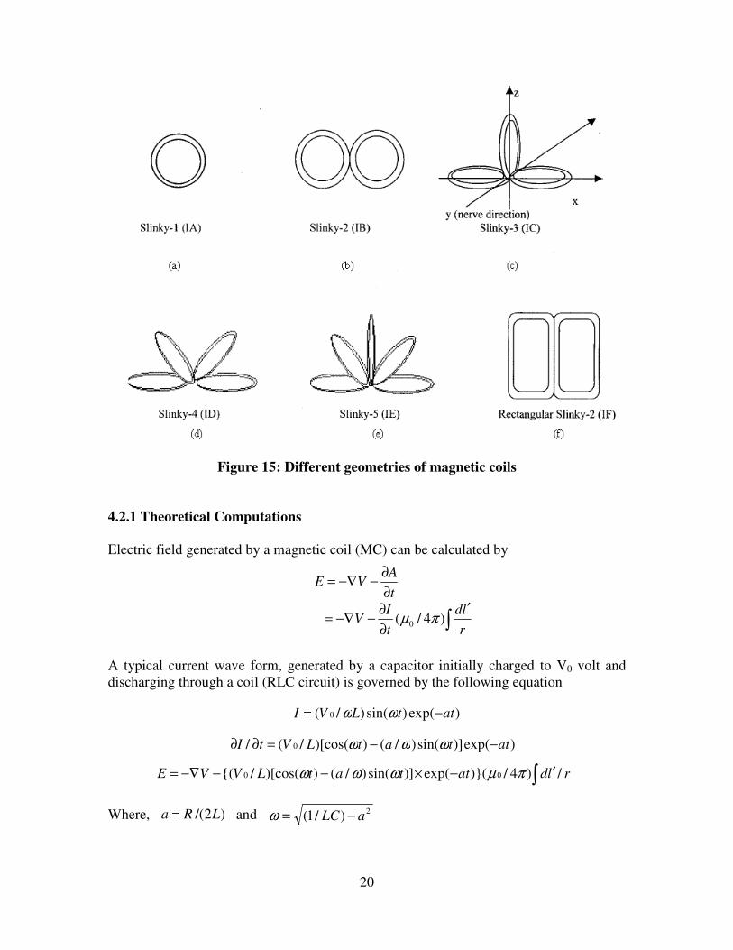
Here we will discuss another paper (Lin, Hsiao, & Dhaka, May 2000). In these paper

coils of various geometric orientations was studied varying radius, number of turns,

slinky, wire length etc. Different geometry of coils that were studied are shown in figure

15.

20

Figure 15: Different geometries of magnetic coils

4.2.1 Theoretical Computations

Electric field generated by a magnetic coil (MC) can be calculated by

A typical current wave form, generated by a capacitor initially charged to V0 volt and

discharging through a coil (RLC circuit) is governed by the following equation

Where, and

t

AVE

∂

∂−−∇=

∫′

∂

∂−−∇=

r

ld

t

IV )4/( 0 πµ

)exp()sin()/( 0 attLVI −= ωω

)exp()]sin()/())[cos(/(/ 0 attatLVtI −−=∂∂ ωωω

∫ ′−×−−−∇= rldattatLVVE /)4/)(exp()]sin()/())[cos(/( 00 πµωωω

)2/( LRa = 2)/1( aLC −=ω

21

For uniform current distribution along the coil becomes insignificant compared to the

other factors. So,

1.

2.

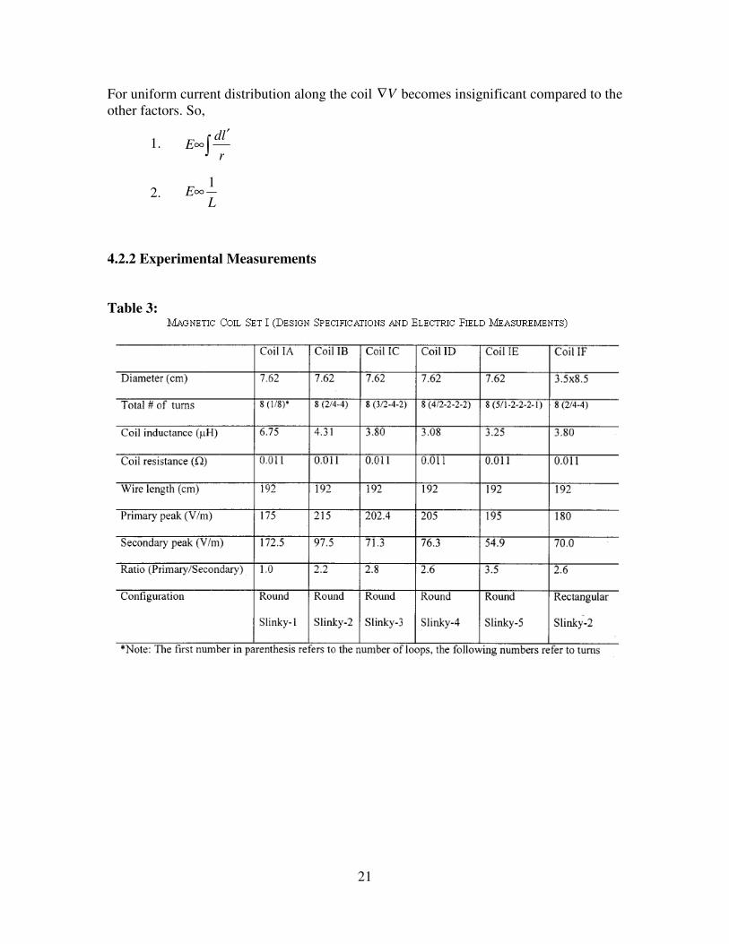
4.2.2 Experimental Measurements

Table 3:

V∇

∫′

∞r

ldE

LE

1∞

22

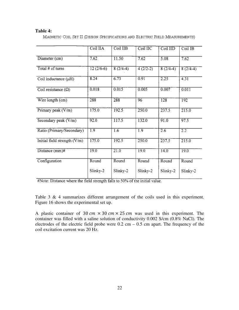
Table 4:

Table 3 & 4 summarizes different arrangement of the coils used in this experiment.

Figure 16 shows the experimental set up.

A plastic container of 30 × 30 × 25 was used in this experiment. The

container was filled with a saline solution of conductivity 0.002 S/cm (0.8% NaCl). The

electrodes of the electric field probe were 0.2 cm – 0.5 cm apart. The frequency of the

coil excitation current was 20 Hz.

23

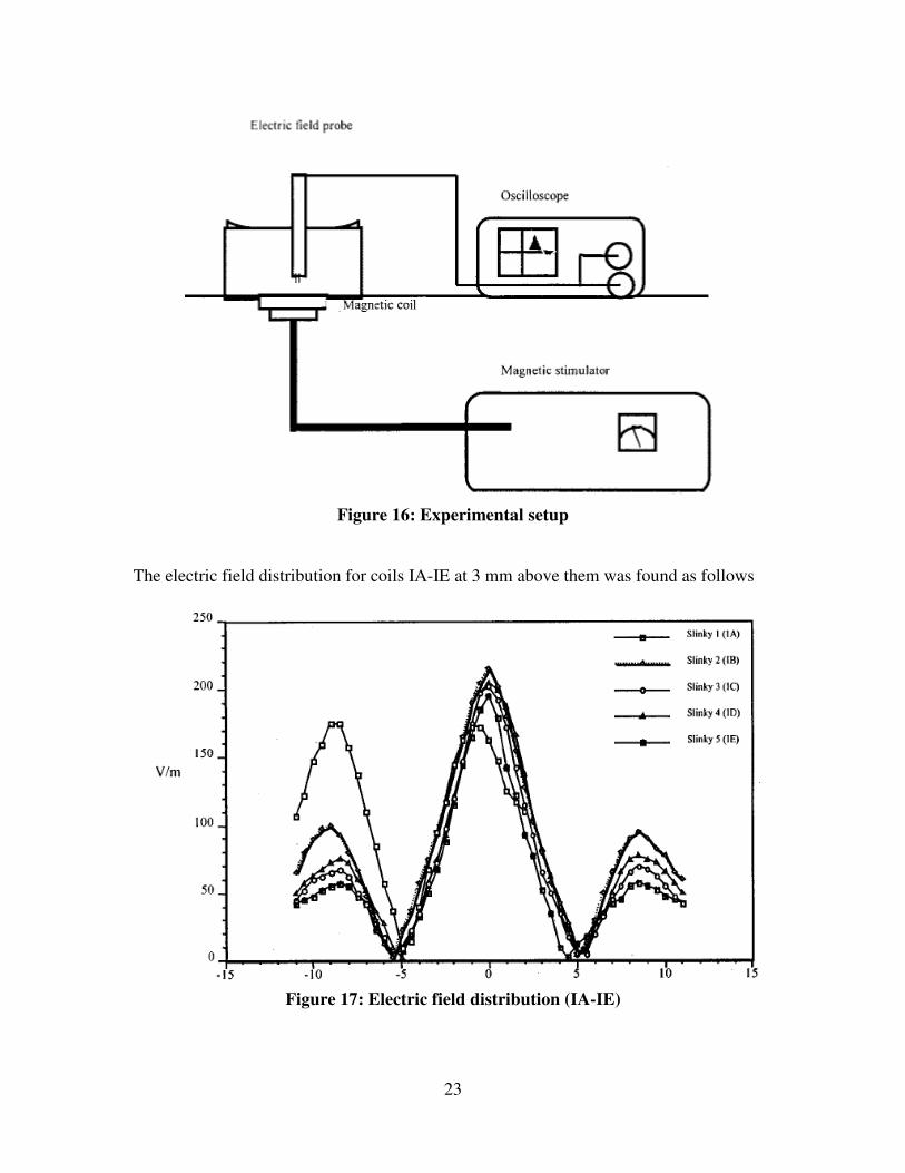
Figure 16: Experimental setup

The electric field distribution for coils IA-IE at 3 mm above them was found as follows

Figure 17: Electric field distribution (IA-IE)

24

From figure 17 we can clearly see that the ratio of NOPQRSPTNUVWXYZSP increases as number of

slinky increases. This happens because with increased number of slinky in other planes

than the horizontal, effective r increases as a result Esecondary decreases.

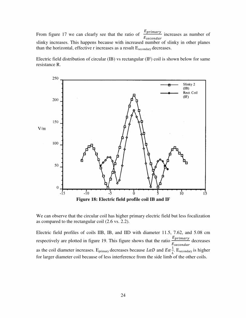
Electric field distribution of circular (IB) vs rectangular (IF) coil is shown below for same

resistance R.

Figure 18: Electric field profile coil IB and IF

We can observe that the circular coil has higher primary electric field but less focalization

as compared to the rectangular coil (2.6 vs. 2.2).

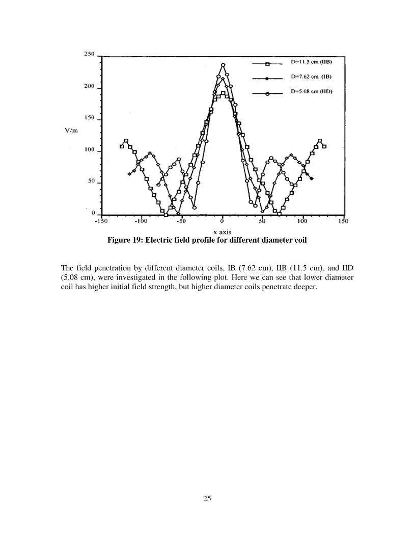
Electric field profiles of coils IIB, IB, and IID with diameter 11.5, 7.62, and 5.08 cm

respectively are plotted in figure 19. This figure shows that the ratio NOPQRSPTNUVWXYZSP decreases

as the coil diameter increases. Eprimary decreases because 3&[ and & D#. Esecondary is higher

for larger diameter coil because of less interference from the side limb of the other coils.

25

Figure 19: Electric field profile for different diameter coil

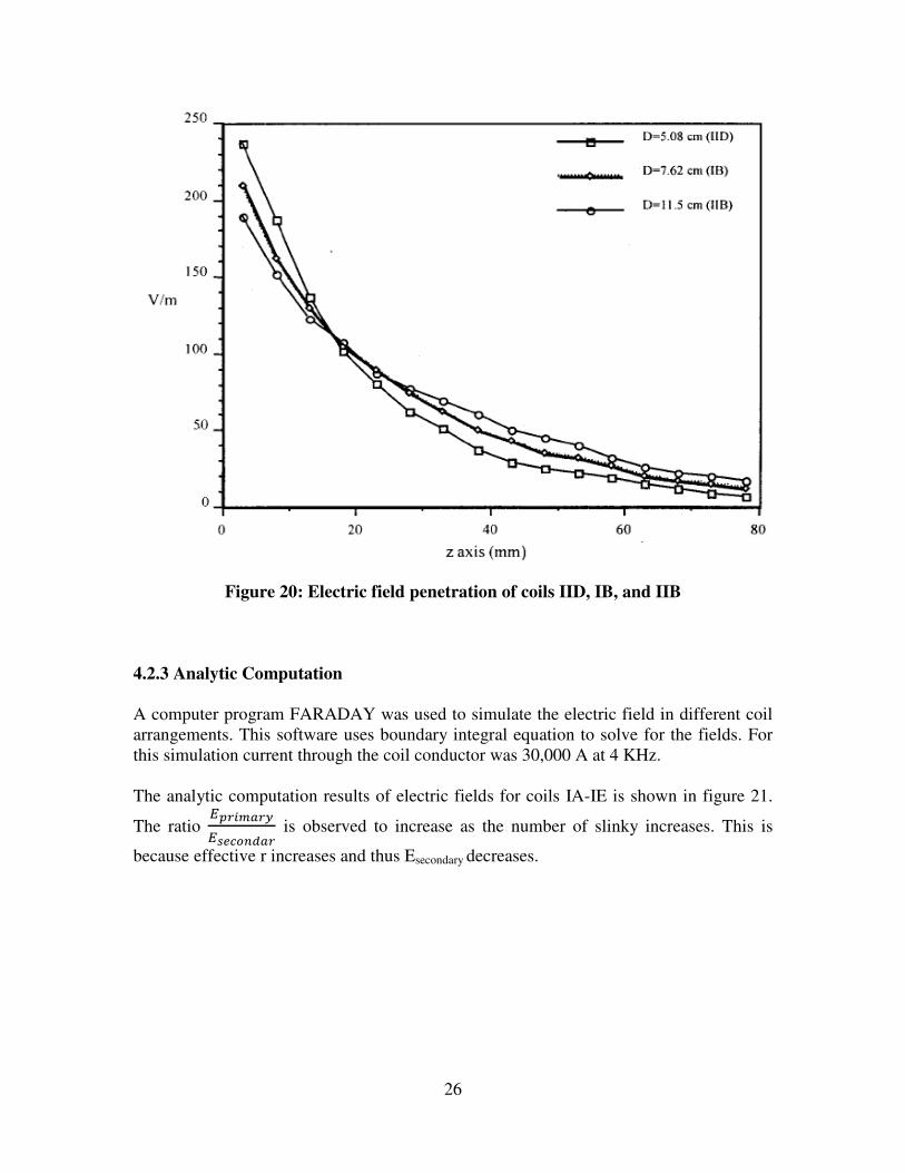
The field penetration by different diameter coils, IB (7.62 cm), IIB (11.5 cm), and IID

(5.08 cm), were investigated in the following plot. Here we can see that lower diameter

coil has higher initial field strength, but higher diameter coils penetrate deeper.

26

Figure 20: Electric field penetration of coils IID, IB, and IIB

4.2.3 Analytic Computation

A computer program FARADAY was used to simulate the electric field in different coil

arrangements. This software uses boundary integral equation to solve for the fields. For

this simulation current through the coil conductor was 30,000 A at 4 KHz.

The analytic computation results of electric fields for coils IA-IE is shown in figure 21.

The ratio NOPQRSPTNUVWXYZSP is observed to increase as the number of slinky increases. This is

because effective r increases and thus Esecondary decreases.

27

Figure 21: Electric field profile of coils IA-IE

Coils IIB, IB, and IID were studied to learn the behavior of different diameter coils. The

diameters were 11.5, 7.62, and 5.08 cm respectively. The initial field strengths were 454,

517, and 789 V/m respectively. So, the smallest diameter coil had the highest field

strength. This happens for the same reason as stated in Art 4.2.2. Eprimary increases

because 3&[ and & D#. Esecondary is higher for larger diameter coil because of less

interference from the side limb of the other coils. The ratio primary to secondary field

was found to be 1.5, 2.0, and 2.3 respectively. So the ratio decreases as the coil diameter

increases, agreeing to the experimental results. But the larger diameter coil maintained a

higher field strength after 30 mm distance.

4.2.4 Findings from (Lin, Hsiao, & Dhaka, May 2000)

Slinky arrangement of coils produces more focalized electric field than the planar circular

coils. Peak primary to secondary electric field ratios were found to be 1, 2.2, 2.85, 2.62,

and 3.54 for coils with slinky 1 to 5 respectively.

Coils with larger diameters have better penetration depth than those with smaller

diameter coils. Coils with less number of turns have higher initial field strength.

5. MY FINDINGS

28

I used XFDTD 6.5 to simulate a homogeneous rectangular phantom of 225 ×150 × 150 . 2 mm shell was used in the phantom that was facing the magnetic

coil. 30,000 A electric current was flowing through the coil conductor at 915 MHz.

Muscle simulating tissue had conductivity 0.97 S/m, relative permittivity of 41.5 and

density 1000 Kg/m3. The shell had conductivity of 0 S/m, relative permittivity of 3.7 and

density 0 Kg/m3. Two coils were placed such that the wires in one edge of a coil were at

the middle of the two wires of the other coil. In this way, we can facilitate maximum

electric field near the intersection of the two coils. The other edges would try to decrease

the effect of the other coil. So, we will be having maximum focused electric field. Each

of the coils had 4 turns and radius of 38.1 mm. The wire had a length of 80 mm and

radius of 0.25 mm. The wire material was selected to perfect electrical conductor (PEC).

The coils were placed such that the nearest coil element was 3 mm away from the tissue.

Base cell size of 1 mm was chosen in all directions. Liao absorbing boundary was used to

simulate.

Figure 22: The phantom and coil arrangement for simulation

Results

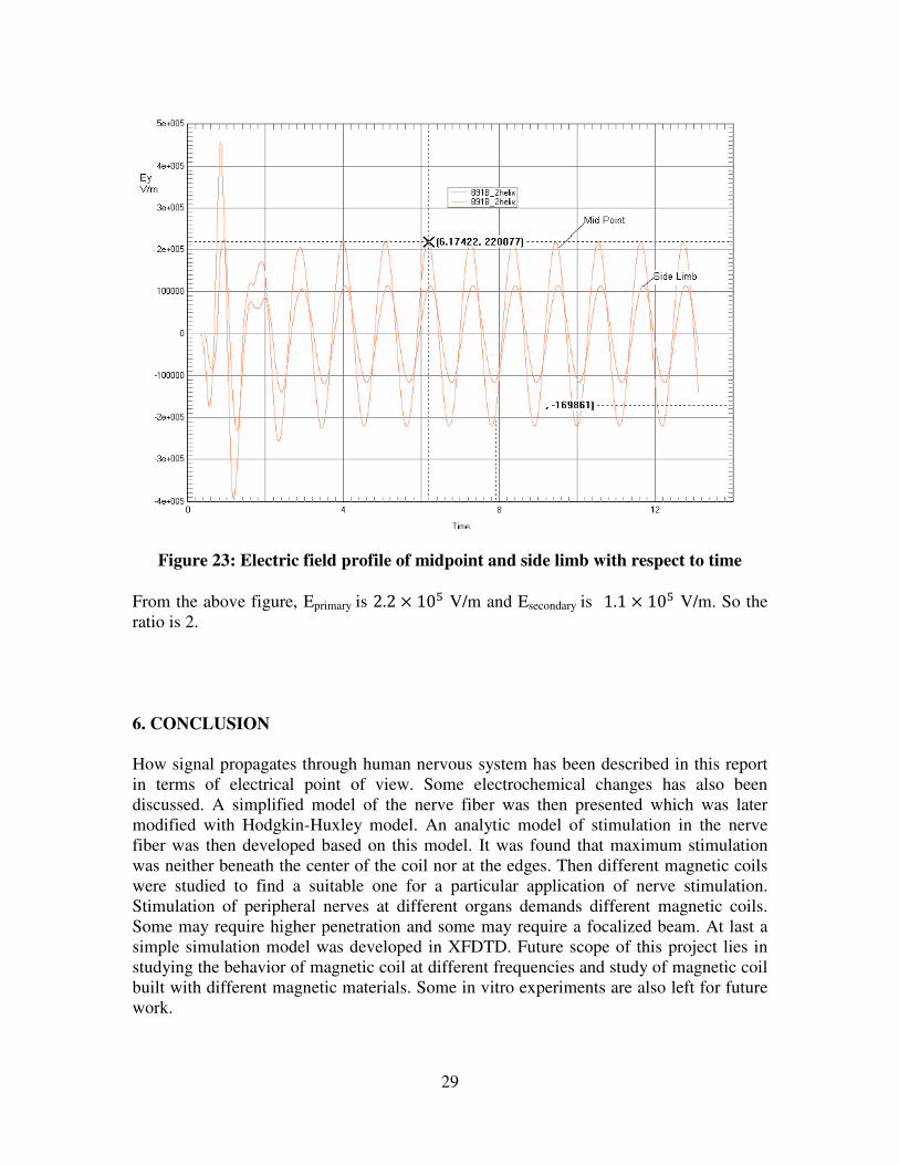
After the simulation was performed the electric field profile at the underneath of the

intersection of the two coils (mid points) and the side edges (side limb) were plotted in

figure 23.

29

Figure 23: Electric field profile of midpoint and side limb with respect to time

From the above figure, Eprimary is 2.2 × 10\ V/m and Esecondary is 1.1 × 10\ V/m. So the

ratio is 2.

6. CONCLUSION

How signal propagates through human nervous system has been described in this report

in terms of electrical point of view. Some electrochemical changes has also been

discussed. A simplified model of the nerve fiber was then presented which was later

modified with Hodgkin-Huxley model. An analytic model of stimulation in the nerve

fiber was then developed based on this model. It was found that maximum stimulation

was neither beneath the center of the coil nor at the edges. Then different magnetic coils

were studied to find a suitable one for a particular application of nerve stimulation.

Stimulation of peripheral nerves at different organs demands different magnetic coils.

Some may require higher penetration and some may require a focalized beam. At last a

simple simulation model was developed in XFDTD. Future scope of this project lies in

studying the behavior of magnetic coil at different frequencies and study of magnetic coil

built with different magnetic materials. Some in vitro experiments are also left for future

work.

30

Bibliography

Davidovits, P. (2007). Physics in Biology and Medicine.

Lin, V. W.-H., Hsiao, I. N., & Dhaka, a. V. (May 2000). Magnetic Coil Design

Considerations for Functional Magnetic Stimulation. IEEE Trans. on Biomed. Eng. , Vol.

47, No. 5.

Roth, B. J., & Basser, P. J. (June 1990). A model of the stimulation of a nerve fibre by

electromagnetic induction. IEEE Transactions on Biomedical Engineering , vol. 37, No.

6.

Spine Universe. (n.d.). Retrieved April 2009, from www.spineuniverse.com