nested markov models...part one: non-parametric identi cation the general identi cation problem for...
TRANSCRIPT
Nested Markov Models
Thomas S. Richardson
Department of StatisticsUniversity of Washington
Center for Causal DiscoveryUniversity of Pittsburgh
20 April 2017
1 / 79
Collaborators
Robin Evans(Oxford)
James Robins(Harvard)
Ilya Shpitser(Johns Hopkins)
2 / 79

Outline
Part One: Non-parametric Identification
Part Two: The Nested Markov Model
3 / 79

Part One: Non-parametric identification
The general identification problem for DAGs with unobservedvariables
Simple examples
Tian’s Algorithm
Formulation in terms of ’Fixing’ operation
4 / 79

Intervention distributions (I)
Given a causal DAG G(V ) with distribution:
p(V ) =∏v∈V
p(v | pa(v))
where pa(v) = {x | x → v};
Intervention distribution on X :
p(V \ X | do(X = x)) =∏
v∈V\X
p(v | pa(v)).
here on the RHS a variable in X occurring in pa(v), for some v ∈ V \ X ,takes the corresponding value in x.
5 / 79

Example
X M Y
L
X M Y
L
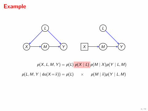
p(X , L,M,Y ) = p(L) p(X | L) p(M | X )p(Y | L,M)
p(L,M,Y | do(X = x)) = p(L) × p(M | x)p(Y | L,M)
6 / 79
Example
X M Y
L
X M Y
L
p(X , L,M,Y ) = p(L) p(X | L) p(M | X )p(Y | L,M)
p(L,M,Y | do(X = x)) = p(L) × p(M | x)p(Y | L,M)
6 / 79

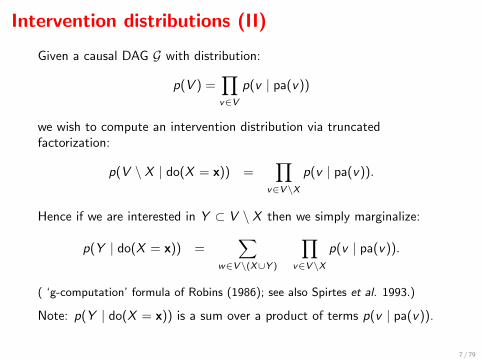
Intervention distributions (II)
Given a causal DAG G with distribution:
p(V ) =∏v∈V
p(v | pa(v))
we wish to compute an intervention distribution via truncatedfactorization:
p(V \ X | do(X = x)) =∏
v∈V\X
p(v | pa(v)).
Hence if we are interested in Y ⊂ V \ X then we simply marginalize:
p(Y | do(X = x)) =∑
w∈V\(X∪Y )
∏v∈V\X
p(v | pa(v)).
( ‘g-computation’ formula of Robins (1986); see also Spirtes et al. 1993.)
Note: p(Y | do(X = x)) is a sum over a product of terms p(v | pa(v)).
7 / 79

Example
X M Y
L
X M Y
L
p(X , L,M,Y ) = p(L)p(X | L)p(M | X )p(Y | L,M)
p(L,M,Y | do(X = x)) = p(L)p(M | x)p(Y | L,M)
p(Y | do(X = x)) =∑l,m
p(L= l)p(M =m | x)p(Y | L= l ,M =m)
Note that p(Y | do(X = x)) 6= p(Y | X = x).
8 / 79

Example
X M Y
L
X M Y
L
p(X , L,M,Y ) = p(L)p(X | L)p(M | X )p(Y | L,M)
p(L,M,Y | do(X = x)) = p(L)p(M | x)p(Y | L,M)
p(Y | do(X = x)) =∑l,m
p(L= l)p(M =m | x)p(Y | L= l ,M =m)
Note that p(Y | do(X = x)) 6= p(Y | X = x).
8 / 79

Example
X M Y
L
X M Y
L
p(X , L,M,Y ) = p(L)p(X | L)p(M | X )p(Y | L,M)
p(L,M,Y | do(X = x)) = p(L)p(M | x)p(Y | L,M)
p(Y | do(X = x)) =∑l,m
p(L= l)p(M =m | x)p(Y | L= l ,M =m)
Note that p(Y | do(X = x)) 6= p(Y | X = x).
8 / 79
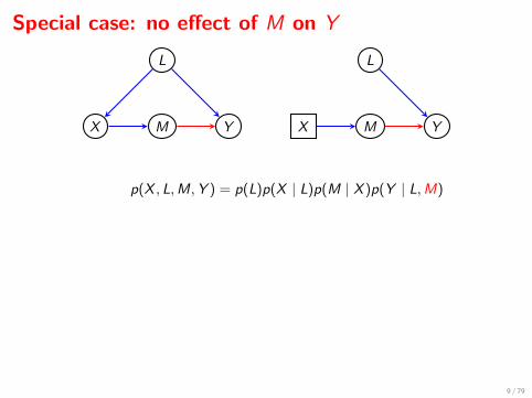
Special case: no effect of M on Y
X M Y
L
X M Y
L
p(X , L,M,Y ) = p(L)p(X | L)p(M | X )p(Y | L,M)
p(L,M,Y | do(X = x)) = p(L)p(M | x)p(Y | L)
p(Y | do(X = x)) =∑l,m
p(L= l)p(M =m | x)p(Y | L= l)
=∑l
p(L= l)p(Y | L= l)
= p(Y ) 6= P(Y | x)
since X 6⊥⊥ Y . ‘Correlation is not Causation’.
9 / 79

Special case: no effect of M on Y
X M Y
L
X M Y
L
p(X , L,M,Y ) = p(L)p(X | L)p(M | X )p(Y | L)
p(L,M,Y | do(X = x)) = p(L)p(M | x)p(Y | L)
p(Y | do(X = x)) =∑l,m
p(L= l)p(M =m | x)p(Y | L= l)
=∑l
p(L= l)p(Y | L= l)
= p(Y ) 6= P(Y | x)
since X 6⊥⊥ Y . ‘Correlation is not Causation’.
9 / 79

Special case: no effect of M on Y
X M Y
L
X M Y
L
p(X , L,M,Y ) = p(L)p(X | L)p(M | X )p(Y | L)
p(L,M,Y | do(X = x)) = p(L)p(M | x)p(Y | L)
p(Y | do(X = x)) =∑l,m
p(L= l)p(M =m | x)p(Y | L= l)
=∑l
p(L= l)p(Y | L= l)
= p(Y ) 6= P(Y | x)
since X 6⊥⊥ Y . ‘Correlation is not Causation’.
9 / 79

Special case: no effect of M on Y
X M Y
L
X M Y
L
p(X , L,M,Y ) = p(L)p(X | L)p(M | X )p(Y | L)
p(L,M,Y | do(X = x)) = p(L)p(M | x)p(Y | L)
p(Y | do(X = x)) =∑l,m
p(L= l)p(M =m | x)p(Y | L= l)
=∑l
p(L= l)p(Y | L= l)
= p(Y ) 6= P(Y | x)
since X 6⊥⊥ Y . ‘Correlation is not Causation’.
9 / 79

Special case: no effect of M on Y
X M Y
L
X M Y
L
p(X , L,M,Y ) = p(L)p(X | L)p(M | X )p(Y | L)
p(L,M,Y | do(X = x)) = p(L)p(M | x)p(Y | L)
p(Y | do(X = x)) =∑l,m
p(L= l)p(M =m | x)p(Y | L= l)
=∑l
p(L= l)p(Y | L= l)
= p(Y ) 6= P(Y | x)
since X 6⊥⊥ Y . ‘Correlation is not Causation’.
9 / 79

Special case: no effect of M on Y
X M Y
L
X M Y
L
p(X , L,M,Y ) = p(L)p(X | L)p(M | X )p(Y | L)
p(L,M,Y | do(X = x)) = p(L)p(M | x)p(Y | L)
p(Y | do(X = x)) =∑l,m
p(L= l)p(M =m | x)p(Y | L= l)
=∑l
p(L= l)p(Y | L= l)
= p(Y ) 6= P(Y | x)
since X 6⊥⊥ Y . ‘Correlation is not Causation’.9 / 79

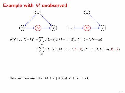
Example with M unobserved
X M Y
L
X M Y
L
p(Y | do(X = x)) =∑l,m
p(L= l)p(M =m | x)p(Y | L= l ,M =m)
=∑l,m
p(L= l)p(M =m | x , L= l)p(Y | L= l ,M =m,X = x)
=∑l,m
p(L= l)p(Y ,M =m | L= l ,X = x)
=∑l
p(L= l)p(Y | L= l ,X = x).
Here we have used that M ⊥⊥ L | X and Y ⊥⊥ X | L,M.
⇒ can find p(Y | do(X = x)) even if M not observed.
This is an example of the ‘back door formula’, aka ‘standardization’.
10 / 79

Example with M unobserved
X M Y
L
X M Y
L
p(Y | do(X = x)) =∑l,m
p(L= l)p(M =m | x)p(Y | L= l ,M =m)
=∑l,m
p(L= l)p(M =m | x , L= l)p(Y | L= l ,M =m,X = x)
=∑l,m
p(L= l)p(Y ,M =m | L= l ,X = x)
=∑l
p(L= l)p(Y | L= l ,X = x).
Here we have used that M ⊥⊥ L | X and Y ⊥⊥ X | L,M.
⇒ can find p(Y | do(X = x)) even if M not observed.
This is an example of the ‘back door formula’, aka ‘standardization’. 10 / 79

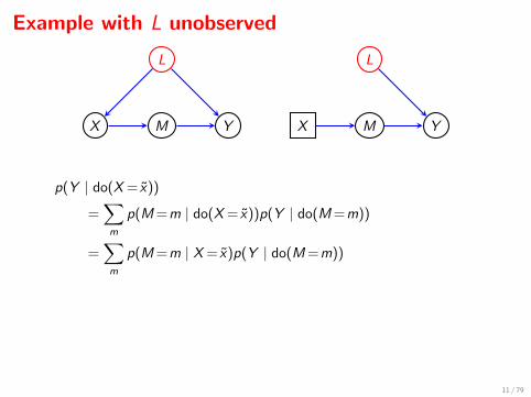
Example with L unobserved
X M Y
L
X M Y
L
p(Y | do(X = x))
=∑m
p(M =m | do(X = x))p(Y | do(M =m))
=∑m
p(M =m | X = x)p(Y | do(M =m))
=∑m
p(M =m | X = x)
(∑x∗
p(X =x∗)p(Y | M =m,X =x∗)
)
⇒ can find p(Y | do(X = x)) even if L not observed.
This is an example of the ‘front door formula’ of Pearl (1995).
11 / 79

Example with L unobserved
X M Y
L
X M Y
L
p(Y | do(X = x))
=∑m
p(M =m | do(X = x))p(Y | do(M =m))
=∑m
p(M =m | X = x)p(Y | do(M =m))
=∑m
p(M =m | X = x)
(∑x∗
p(X =x∗)p(Y | M =m,X =x∗)
)
⇒ can find p(Y | do(X = x)) even if L not observed.
This is an example of the ‘front door formula’ of Pearl (1995).11 / 79

But with both L and M unobserved....
X M Y
L
...we are out of luck!
Given P(X ,Y ), absent further assumptions we cannot distinguish:
X Y
L
X M Y
12 / 79

But with both L and M unobserved....
X M Y
L
...we are out of luck!
Given P(X ,Y ), absent further assumptions we cannot distinguish:
X Y
L
X M Y
12 / 79
General Identification Question
Given: a latent DAG G(O ∪H), where O are observed, H are hidden, anddisjoint subsets X ,Y ⊆ O.
Q: Is p(Y | do(X )) identified given p(O)?
A: Provide either an identifying formula that is a function of p(O)
or report that p(Y | do(X )) is not identified.
Motivations:
Characterize which interventions can be identified withoutparametric assumptions;
Understand which functionals of the observed margin have a causalinterpretation;
13 / 79

Latent ProjectionCan preserve conditional independences and causal coherence withlatents using paths. DAG G on vertices V = O∪H, define latentprojection as follows: (Verma and Pearl, 1992)
Whenever there is a path of the form
x h1 · · · hk y
add
x y
Whenever there is a path of the form
x h1 · · · hk y
add
x y
Then remove all latent variables H from the graph.
14 / 79

Latent ProjectionCan preserve conditional independences and causal coherence withlatents using paths. DAG G on vertices V = O∪H, define latentprojection as follows: (Verma and Pearl, 1992)
Whenever there is a path of the form
x h1 · · · hk y
add
x y
Whenever there is a path of the form
x h1 · · · hk y
add
x y
Then remove all latent variables H from the graph.14 / 79

ADMGs
u
x
y
z
w t
−→project
x
y
z
t
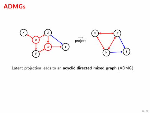
Latent projection leads to an acyclic directed mixed graph (ADMG)
Can read off independences with d/m-separation.
The projection preserves the causal structure; Verma and Pearl (1992).
15 / 79
ADMGs
u
x
y
z
w t
−→project
x
y
z
t
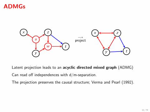
Latent projection leads to an acyclic directed mixed graph (ADMG)
Can read off independences with d/m-separation.
The projection preserves the causal structure; Verma and Pearl (1992).
15 / 79
ADMGs
u
x
y
z
w t
−→project
x
y
z
t
Latent projection leads to an acyclic directed mixed graph (ADMG)
Can read off independences with d/m-separation.
The projection preserves the causal structure; Verma and Pearl (1992).
15 / 79

‘Conditional’ Acyclic Directed Mixed Graphs
An ‘conditional’ acyclic directed mixed graph (CADMG) is a bi-partitegraph G(V ,W ), used to represent structure of a distribution over V ,indexed by W , for example P(V | do(W )).
We require:
(i) The induced subgraph of G on V is an ADMG;
(ii) The induced subgraph of G on W contains no edges;
(iii) Edges between vertices in W and V take the form w → v .
We represent V with circles, W with squares:
A0 L1 A1 Y
Here V = {L1,Y } and W = {A0,A1}.
16 / 79
Ancestors and Descendants
L0 A0 L1 A1 Y
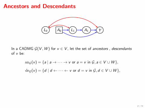
In a CADMG G(V ,W ) for v ∈ V , let the set of ancestors , descendantsof v be:
anG(v) = {a | a→ · · · → v or a = v in G, a ∈ V ∪W },
deG(v) = {d | d ← · · · ← v or d = v in G, d ∈ V ∪W },
In the example above:
an(y) = {a0, l1, a1, y}.
17 / 79

Ancestors and Descendants
L0 A0 L1 A1 Y
In a CADMG G(V ,W ) for v ∈ V , let the set of ancestors , descendantsof v be:
anG(v) = {a | a→ · · · → v or a = v in G, a ∈ V ∪W },
deG(v) = {d | d ← · · · ← v or d = v in G, d ∈ V ∪W },
In the example above:
an(y) = {a0, l1, a1, y}.
17 / 79
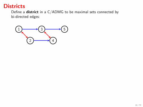
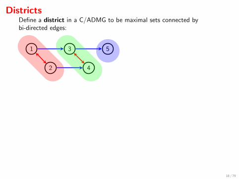
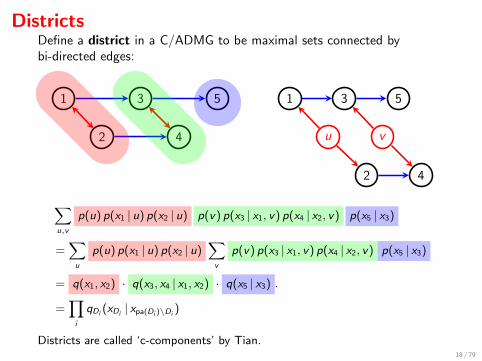
DistrictsDefine a district in a C/ADMG to be maximal sets connected bybi-directed edges:
1
2
3
4
5
1 3 5
u v
2 4
∑u,v
p(u) p(x1 | u) p(x2 | u) p(v) p(x3 | x1, v) p(x4 | x2, v) p(x5 | x3)
=∑u
p(u) p(x1 | u) p(x2 | u)∑v
p(v) p(x3 | x1, v) p(x4 | x2, v) p(x5 | x3)
= q(x1, x2) · q(x3, x4 | x1, x2) · q(x5 | x3) .
=∏i
qDi (xDi | xpa(Di )\Di)
Districts are called ‘c-components’ by Tian.
18 / 79

DistrictsDefine a district in a C/ADMG to be maximal sets connected bybi-directed edges:
1
2
3
4
5 1 3 5
u v
2 4
∑u,v
p(u) p(x1 | u) p(x2 | u) p(v) p(x3 | x1, v) p(x4 | x2, v) p(x5 | x3)
=∑u
p(u) p(x1 | u) p(x2 | u)∑v
p(v) p(x3 | x1, v) p(x4 | x2, v) p(x5 | x3)
= q(x1, x2) · q(x3, x4 | x1, x2) · q(x5 | x3) .
=∏i
qDi (xDi | xpa(Di )\Di)
Districts are called ‘c-components’ by Tian.
18 / 79
DistrictsDefine a district in a C/ADMG to be maximal sets connected bybi-directed edges:
1
2
3
4
5 1 3 5
u v
2 4
∑u,v
p(u) p(x1 | u) p(x2 | u) p(v) p(x3 | x1, v) p(x4 | x2, v) p(x5 | x3)
=∑u
p(u) p(x1 | u) p(x2 | u)∑v
p(v) p(x3 | x1, v) p(x4 | x2, v) p(x5 | x3)
= q(x1, x2) · q(x3, x4 | x1, x2) · q(x5 | x3) .
=∏i
qDi (xDi | xpa(Di )\Di)
Districts are called ‘c-components’ by Tian.18 / 79
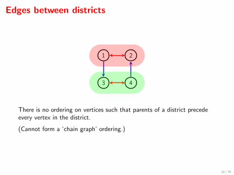
Edges between districts
1 2
3 4
There is no ordering on vertices such that parents of a district precedeevery vertex in the district.
(Cannot form a ‘chain graph’ ordering.)
19 / 79

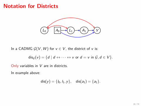
Notation for Districts
L0 A0 L1 A1 Y
In a CADMG G(V ,W ) for v ∈ V , the district of v is:
disG(v) = {d | d ↔ · · · ↔ v or d = v in G, d ∈ V }.
Only variables in V are in districts.
In example above:
dis(y) = {l0, l1, y}, dis(a1) = {a1}.
We use D(G) to denote the set of districts in G.
In example D(G) = { {l0, l1, y}, {a1} }.
20 / 79

Notation for Districts
L0 A0 L1 A1 Y
In a CADMG G(V ,W ) for v ∈ V , the district of v is:
disG(v) = {d | d ↔ · · · ↔ v or d = v in G, d ∈ V }.
Only variables in V are in districts.
In example above:
dis(y) = {l0, l1, y}, dis(a1) = {a1}.
We use D(G) to denote the set of districts in G.
In example D(G) = { {l0, l1, y}, {a1} }.20 / 79

Tian’s ID algorithm for identifying P(Y | do(X ))
Jin Tian
(A) Re-express the query as a sum over a product of interventiondistributions on districts:
p(Y | do(X )) =∑∏
i
p(Di | do(pa(Di ) \ Di )).
(B) Check whether each term: p(Di | do(pa(Di ) \ Di )) is identified.
This is clearly sufficient for identifiability.
Necessity follows from results of Shpitser (2006); see also Huang andValtorta (2006).
21 / 79

(A) Decomposing the query
1 Remove edges into X :Let G[V \ X ] denote the graph formed by removing edges with anarrowhead into X .
2 Restrict to variables that are (still) ancestors of Y :Let T = anG[V\X ](Y )be vertices that lie on directed paths between X and Y (aftercutting edges into X ).Let G∗ be formed from G[V \ X ] by removing vertices not in T .
3 Find the districts:Let D1, . . . ,Ds be the districts in G∗.
Then:
P(Y | do(X )) =∑
T\(X∪Y )
∏Di
p(Di | do(pa(Di ) \ Di )).
22 / 79

(A) Decomposing the query
1 Remove edges into X :Let G[V \ X ] denote the graph formed by removing edges with anarrowhead into X .
2 Restrict to variables that are (still) ancestors of Y :Let T = anG[V\X ](Y )be vertices that lie on directed paths between X and Y (aftercutting edges into X ).
Let G∗ be formed from G[V \ X ] by removing vertices not in T .
3 Find the districts:Let D1, . . . ,Ds be the districts in G∗.
Then:
P(Y | do(X )) =∑
T\(X∪Y )
∏Di
p(Di | do(pa(Di ) \ Di )).
22 / 79

(A) Decomposing the query
1 Remove edges into X :Let G[V \ X ] denote the graph formed by removing edges with anarrowhead into X .
2 Restrict to variables that are (still) ancestors of Y :Let T = anG[V\X ](Y )be vertices that lie on directed paths between X and Y (aftercutting edges into X ).Let G∗ be formed from G[V \ X ] by removing vertices not in T .
3 Find the districts:Let D1, . . . ,Ds be the districts in G∗.
Then:
P(Y | do(X )) =∑
T\(X∪Y )
∏Di
p(Di | do(pa(Di ) \ Di )).
22 / 79

(A) Decomposing the query
1 Remove edges into X :Let G[V \ X ] denote the graph formed by removing edges with anarrowhead into X .
2 Restrict to variables that are (still) ancestors of Y :Let T = anG[V\X ](Y )be vertices that lie on directed paths between X and Y (aftercutting edges into X ).Let G∗ be formed from G[V \ X ] by removing vertices not in T .
3 Find the districts:Let D1, . . . ,Ds be the districts in G∗.
Then:
P(Y | do(X )) =∑
T\(X∪Y )
∏Di
p(Di | do(pa(Di ) \ Di )).
22 / 79

Example: front door graph
X M Y
p(Y | do(X ))
G
X M Y
G[V\{X}] = G∗
T = {X ,M,Y }
Districts in T \ {X} are D1 = {M}, D2 = {Y }.
p(Y | do(X )) =∑M
p(M | do(X ))p(Y | do(M))
23 / 79

Example: front door graph
X M Y
p(Y | do(X ))
G
X M Y
G[V\{X}] = G∗
T = {X ,M,Y }
Districts in T \ {X} are D1 = {M}, D2 = {Y }.
p(Y | do(X )) =∑M
p(M | do(X ))p(Y | do(M))
23 / 79

Example: front door graph
X M Y
p(Y | do(X ))
G
X M Y
G[V\{X}] = G∗
T = {X ,M,Y }
Districts in T \ {X} are D1 = {M}, D2 = {Y }.
p(Y | do(X )) =∑M
p(M | do(X ))p(Y | do(M))
23 / 79
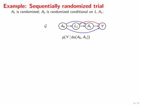
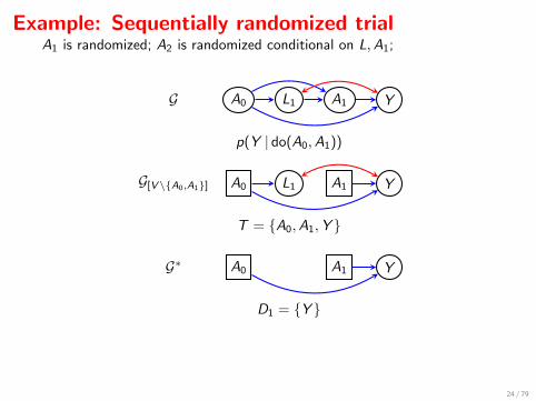
Example: Sequentially randomized trialA1 is randomized; A2 is randomized conditional on L,A1;
A0 L1 A1 YG
p(Y | do(A0,A1))
A0 L1 A1 Y
T = {A0,A1,Y }
G[V\{A0,A1}]
A0 A1 Y
D1 = {Y }
G∗
(Here the decomposition is trivial since there is only one district and nosummation.)
24 / 79

Example: Sequentially randomized trialA1 is randomized; A2 is randomized conditional on L,A1;
A0 L1 A1 YG
p(Y | do(A0,A1))
A0 L1 A1 Y
T = {A0,A1,Y }
G[V\{A0,A1}]
A0 A1 Y
D1 = {Y }
G∗
(Here the decomposition is trivial since there is only one district and nosummation.)
24 / 79
Example: Sequentially randomized trialA1 is randomized; A2 is randomized conditional on L,A1;
A0 L1 A1 YG
p(Y | do(A0,A1))
A0 L1 A1 Y
T = {A0,A1,Y }
G[V\{A0,A1}]
A0 A1 Y
D1 = {Y }
G∗
(Here the decomposition is trivial since there is only one district and nosummation.)
24 / 79

Example: Sequentially randomized trialA1 is randomized; A2 is randomized conditional on L,A1;
A0 L1 A1 YG
p(Y | do(A0,A1))
A0 L1 A1 Y
T = {A0,A1,Y }
G[V\{A0,A1}]
A0 A1 Y
D1 = {Y }
G∗
(Here the decomposition is trivial since there is only one district and nosummation.)
24 / 79

(B) Finding if P(D |do(pa(D) \ D)) is identifiedIdea: Find an ordering r1, . . . , rp of O \ D such that:
If P(O \ {r1, . . . , rt−1} | do(r1, . . . , rt−1)) is identified
Then P(O \ {r1, . . . , rt} | do(r1, . . . , rt)) is also identified.
Sufficient for identifiability of P(D | do(pa(D) \ D)), since:
P(O) is identified
D = O \ {r1, . . . , rp}, soP(O \ {r1, . . . , rp} | do(r1, . . . , rp)) = P(D | do(pa(D) \ D)).
Such a vertex rt will said to be ‘fixable’, given that we have already‘fixed’ r1, . . . , rt−1:
‘fixing’ differs formally from ‘do’/cutting edges since the latter does notpreserve identifiability in general.
To do:
Give a graphical characterization of ‘fixability’;
Construct the identifying formula.
25 / 79

(B) Finding if P(D |do(pa(D) \ D)) is identifiedIdea: Find an ordering r1, . . . , rp of O \ D such that:
If P(O \ {r1, . . . , rt−1} | do(r1, . . . , rt−1)) is identified
Then P(O \ {r1, . . . , rt} | do(r1, . . . , rt)) is also identified.
Sufficient for identifiability of P(D | do(pa(D) \ D)), since:
P(O) is identified
D = O \ {r1, . . . , rp}, soP(O \ {r1, . . . , rp} | do(r1, . . . , rp)) = P(D | do(pa(D) \ D)).
Such a vertex rt will said to be ‘fixable’, given that we have already‘fixed’ r1, . . . , rt−1:
‘fixing’ differs formally from ‘do’/cutting edges since the latter does notpreserve identifiability in general.
To do:
Give a graphical characterization of ‘fixability’;
Construct the identifying formula.25 / 79

The set of fixable vertices
Given a CADMG G(V ,W ) we define the set of fixable vertices,
F (G) ≡ {v | v ∈ V , disG(v) ∩ deG(v) = {v}} .
In words, a vertex v ∈ V is fixable in G if there is no (proper) descendantof v that is in the same district as v in G.
Thus v is fixable if there is no vertex y 6= v such that
v ↔ · · · ↔ y and v → · · · → y in G.
Note that the set of fixable vertices is a subset of V , and contains atleast one vertex from each district in G.
26 / 79

Example: Front door graph
X M Y
G
F (G) = {M,Y }
X is not fixable since Y is a descendant of X and
Y is in the same district as X
27 / 79

Example: Sequentially randomized trial
A0 L1 A1 Y
Here F (G) = {A0,A1,Y }.
L1 is not fixable since Y is a descendant of L1 and
Y is in the same district as L1.
28 / 79

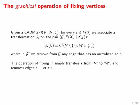
The graphical operation of fixing vertices
Given a CADMG G(V ,W ,E ), for every r ∈ F (G) we associate atransformation φr on the pair (G,P(XV | XW )):
φr (G) ≡ G†(V \ {r},W ∪ {r}),
where in G† we remove from G any edge that has an arrowhead at r .
The operation of ‘fixing r ’ simply transfers r from ‘V ’ to ‘W ’, andremoves edges r ↔ or r ←.
29 / 79

Example: front door graph
X M YG
F (G) = {M,Y }
X M YφM(G)
F (φM(G)) = {X ,Y }
Note that X was not fixable in G,
but it is fixable in φM(G) after fixing M.
30 / 79
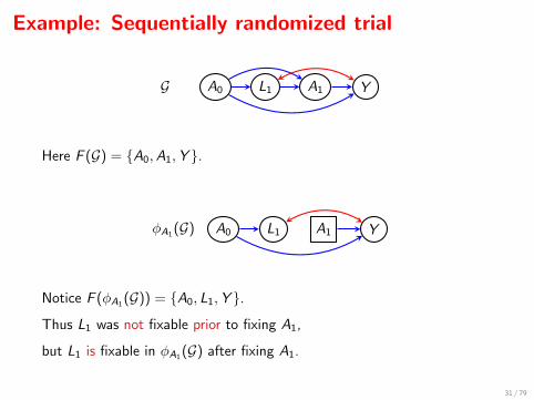
Example: Sequentially randomized trial
A0 L1G A1 Y
Here F (G) = {A0,A1,Y }.
A0 L1φA1 (G) A1 Y
Notice F (φA1 (G)) = {A0, L1,Y }.
Thus L1 was not fixable prior to fixing A1,
but L1 is fixable in φA1 (G) after fixing A1.
31 / 79

The probabilistic operation of fixing vertices
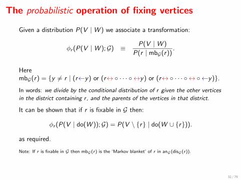
Given a distribution P(V |W ) we associate a transformation:
φr (P(V |W );G) ≡ P(V |W )
P(r | mbG(r)).
HerembG(r) = {y 6= r | (r←y) or (r↔◦ · · · ◦ ↔y) or (r↔◦ · · · ◦ ↔ ◦←y)}.
In words: we divide by the conditional distribution of r given the other vertices
in the district containing r , and the parents of the vertices in that district.
It can be shown that if r is fixable in G then:
φr (P(V | do(W ));G) = P(V \ {r} | do(W ∪ {r})).
as required.
Note: If r is fixable in G then mbG(r) is the ‘Markov blanket’ of r in anG(disG(r)).
32 / 79
The probabilistic operation of fixing vertices
Given a distribution P(V |W ) we associate a transformation:
φr (P(V |W );G) ≡ P(V |W )
P(r | mbG(r)).
HerembG(r) = {y 6= r | (r←y) or (r↔◦ · · · ◦ ↔y) or (r↔◦ · · · ◦ ↔ ◦←y)}.
In words: we divide by the conditional distribution of r given the other vertices
in the district containing r , and the parents of the vertices in that district.
It can be shown that if r is fixable in G then:
φr (P(V | do(W ));G) = P(V \ {r} | do(W ∪ {r})).
as required.
Note: If r is fixable in G then mbG(r) is the ‘Markov blanket’ of r in anG(disG(r)).
32 / 79

Unifying Marginalizing and Conditioning
Some special cases:
If mbG(r) = (V ∪W ) \ {r} then fixing corresponds to marginalizing:
φr (P(V |W );G) =P(V |W )
P(r | (V ∪W ) \ {r})= P(V \ {r} |W )
If mbG(r) = W then fixing corresponds to ordinary conditioning:
φr (P(V |W );G) =P(V |W )
P(r |W )= P(V \ {r} |W ∪ {r})
In the general case fixing corresponds to re-weighting, so
φr (P(V |W );G) = P∗(V \ {r} |W ∪ {r}) 6= P(V \ {r} |W ∪ {r})
Having a single operation simplifies the identification algorithm.
33 / 79

Composition of fixing operations
We use ◦ to indicate composition of operations in the natural way.
If s is fixable in G and then r is fixable in φs(G) (after fixing s) then:
φr ◦ φs(G) ≡ φr (φs(G))
φr ◦ φs(P(V |W );G) ≡ φr (φs (P(V |W );G) ;φs(G))
34 / 79

Back to step (B) of identification
Recall our goal is to identify P(D | do(pa(D) \ D)), for the districts D inG∗:
X M Y
p(Y | do(X ))
G
X M Y
G[V\{X}] = G∗
T = {X ,M,Y }
Districts in T \ {X} are D1 = {M}, D2 = {Y }.
p(Y | do(X )) =∑M
p(M | do(X ))p(Y | do(M))
35 / 79

Back to step (B) of identification
Recall our goal is to identify P(D | do(pa(D) \ D)), for the districts D inG∗:
X M Y
p(Y | do(X ))
G
X M Y
G[V\{X}] = G∗
T = {X ,M,Y }
Districts in T \ {X} are D1 = {M}, D2 = {Y }.
p(Y | do(X )) =∑M
p(M | do(X ))p(Y | do(M))
35 / 79

Example: front door graph: D1 = {M}
X M YG
F (G) = {M,Y }
X M YφY (G)
F (φY (G)) = {X ,M}
X M YφX ◦ φY (G)
This proves that p(M | do(X )) is identified.
36 / 79

Example: front door graph: D2 = {Y }
X M YG
F (G) = {M,Y }
X M YφM(G)
F (φM(G)) = {X ,Y }
X M YφX ◦ φM(G)
This proves that p(Y | do(M)) is identified.
37 / 79
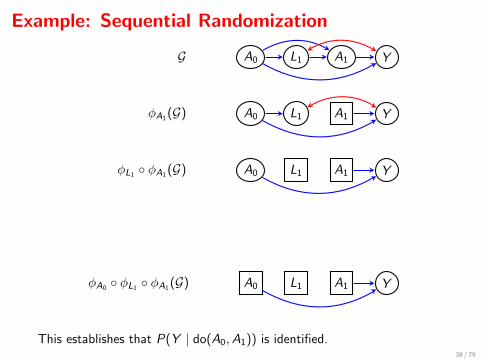
Example: Sequential Randomization
A0 L1G A1 Y
A0 L1φA1 (G) A1 Y
A0 L1φL1 ◦ φA1 (G) A1 Y
A0 L1φA0 ◦ φL1 ◦ φA1 (G) A1 Y
This establishes that P(Y | do(A0,A1)) is identified.38 / 79
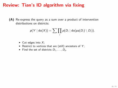
Review: Tian’s ID algorithm via fixing
(A) Re-express the query as a sum over a product of interventiondistributions on districts:
p(Y | do(X )) =∑∏
i
p(Di | do(pa(Di ) \ Di )).
I Cut edges into X ;I Restrict to vertices that are (still) ancestors of Y ;I Find the set of districts D1, . . . ,Dp.
(B) Check whether each term: p(Di | do(pa(Di ) \ Di )) is identified:I Iteratively find a vertex that rt that is fixable in φrt−1 ◦ · · · ◦ φr1 (G),
with rt /∈ Di ;I If no such vertex exists then P(Di | do(pa(Di ) \Di )) is not identified.
39 / 79
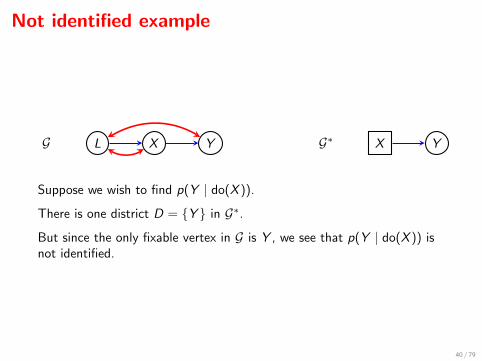
Not identified example
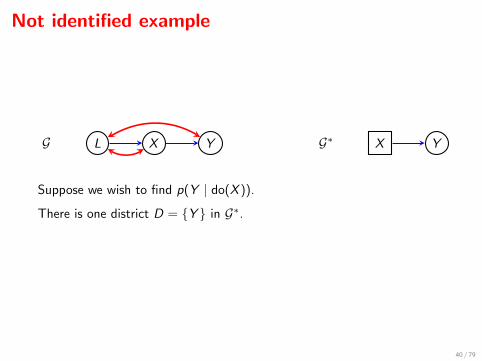
L X YG X YG∗
Suppose we wish to find p(Y | do(X )).
There is one district D = {Y } in G∗.
But since the only fixable vertex in G is Y , we see that p(Y | do(X )) isnot identified.
40 / 79
Not identified example
L X YG X YG∗
Suppose we wish to find p(Y | do(X )).
There is one district D = {Y } in G∗.
But since the only fixable vertex in G is Y , we see that p(Y | do(X )) isnot identified.
40 / 79

Reachable subgraphs of an ADMG
A CADMG G(V ,W ) is reachable from ADMG G∗(V ∪W ) if there is anordering of the vertices in W = 〈w1, . . . ,wk〉, such that for j = 1, . . . , k,
w1 ∈ F (G∗) and for j = 2, . . . , k ,
wj ∈ F (φwj−1 ◦ · · · ◦ φw1 (G∗)).
Thus a subgraph is reachable if, under some ordering, each of the verticesin W may be fixed, first in G∗, and then in φw1 (G∗), then inφw2 (φw1 (G∗)), and so on.
41 / 79

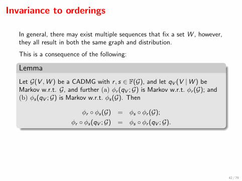
Invariance to orderings
In general, there may exist multiple sequences that fix a set W , however,they all result in both the same graph and distribution.
This is a consequence of the following:
Lemma
Let G(V ,W ) be a CADMG with r , s ∈ F(G), and let qV (V |W ) beMarkov w.r.t. G, and further (a) φr (qV ;G) is Markov w.r.t. φr (G); and(b) φs(qV ;G) is Markov w.r.t. φs(G). Then
φr ◦ φs(G) = φs ◦ φr (G);
φr ◦ φs(qV ;G) = φs ◦ φr (qV ;G).
Consequently, if G(V ,W ) is reachable from G(V ∪W ) thenφV (p(V ,W );G) is uniquely defined.
42 / 79

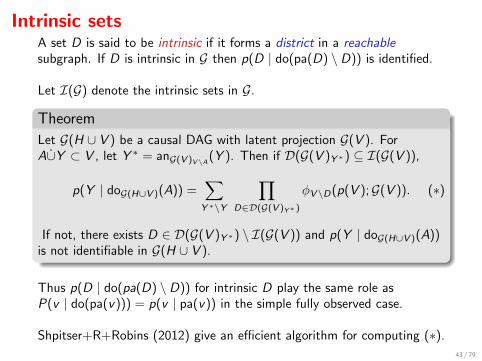
Intrinsic setsA set D is said to be intrinsic if it forms a district in a reachablesubgraph. If D is intrinsic in G then p(D | do(pa(D) \ D)) is identified.
Let I(G) denote the intrinsic sets in G.
Theorem
Let G(H ∪ V ) be a causal DAG with latent projection G(V ). ForA∪Y ⊂ V , let Y ∗ = anG(V )V\A(Y ). Then if D(G(V )Y ∗) ⊆ I(G(V )),
p(Y | doG(H∪V )(A)) =∑Y ∗\Y
∏D∈D(G(V )Y∗ )
φV\D(p(V );G(V )). (∗)
If not, there exists D ∈ D(G(V )Y ∗) \ I(G(V )) and p(Y | doG(H∪V )(A))is not identifiable in G(H ∪ V ).
Thus p(D | do(pa(D) \ D)) for intrinsic D play the same role asP(v | do(pa(v))) = p(v | pa(v)) in the simple fully observed case.
Shpitser+R+Robins (2012) give an efficient algorithm for computing (∗).
43 / 79
Part Two: The Nested Markov Model
1 Motivation
2 Deriving constraints via fixing
3 The Nested Markov Model
4 Finer Factorizations
5 Discrete Parameterization
6 Testing and Fitting
7 Completeness
44 / 79

Outline
1 Motivation
2 Deriving constraints via fixing
3 The Nested Markov Model
4 Finer Factorizations
5 Discrete Parameterization
6 Testing and Fitting
7 Completeness
45 / 79

Motivation
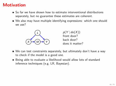
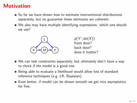
So far we have shown how to estimate interventional distributionsseparately, but no guarantee these estimates are coherent.
We also may have multiple identifying expressions: which one shouldwe use?
X M Y
L p(Y | do(X ))front door?back door?does it matter?
We can test constraints separately, but ultimately don’t have a wayto check if the model is a good one.
Being able to evaluate a likelihood would allow lots of standardinference techniques (e.g. LR, Bayesian).
Even better, if model can be shown smooth we get nice asymptoticsfor free.
All this suggests we should define a model which we can parameterize.
46 / 79

Motivation
So far we have shown how to estimate interventional distributionsseparately, but no guarantee these estimates are coherent.
We also may have multiple identifying expressions: which one shouldwe use?
X M Y
L p(Y | do(X ))front door?back door?does it matter?
We can test constraints separately, but ultimately don’t have a wayto check if the model is a good one.
Being able to evaluate a likelihood would allow lots of standardinference techniques (e.g. LR, Bayesian).
Even better, if model can be shown smooth we get nice asymptoticsfor free.
All this suggests we should define a model which we can parameterize.
46 / 79

Outline
1 Motivation
2 Deriving constraints via fixing
3 The Nested Markov Model
4 Finer Factorizations
5 Discrete Parameterization
6 Testing and Fitting
7 Completeness
47 / 79

Deriving constraints via fixing
Let p(O) be the observed margin from a DAG with latents G(O ∪ H),
Idea: If r ∈ O is fixable then φr (p(O);G) will obey the Markov propertyfor the graph φr (G).
. . . and this can be iterated.
This gives non-parametric constraints that are not independences, thatare implied by the latent DAG.
48 / 79

Example: The ‘Verma’ Constraint
A0 L1G A1 Y
This graph implies no conditional independences on P(A0, L1,A1,Y ).
But since F (G) = {A0,A1,Y }, we may construct:
A0 L1φA1 (G) A1 Y
φA1 (p(A0, L1,A1,Y )) = p(A0, L1,A1,Y )/p(A1 | A0, L1)
A0 ⊥⊥ Y | A1 [φA1 (p(A0, L1,A1,Y );G)]
49 / 79

Example: The ‘Verma’ Constraint
A0 L1G A1 Y
This graph implies no conditional independences on P(A0, L1,A1,Y ).
But since F (G) = {A0,A1,Y }, we may construct:
A0 L1φA1 (G) A1 Y
φA1 (p(A0, L1,A1,Y )) = p(A0, L1,A1,Y )/p(A1 | A0, L1)
A0 ⊥⊥ Y | A1 [φA1 (p(A0, L1,A1,Y );G)]
49 / 79
Outline
1 Motivation
2 Deriving constraints via fixing
3 The Nested Markov Model
4 Finer Factorizations
5 Discrete Parameterization
6 Testing and Fitting
7 Completeness
50 / 79

The nested Markov model
These independences may be used to define a graphical model:
Definition
p(V ) obeys the global nested Markov property for G if for all reachablesets R, the kernel φV\R(p(V );G) obeys the global Markov property forφV\R(G).
This is a ‘generalized’ Markov property since it is defined by conditionalindependence in re-weighted distributions (obtained via fixing).
We will use N (G) to indicate the set of distributions obeying thisproperty.
51 / 79

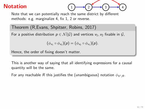
Notation 1 2 3 4
Note that we can potentially reach the same district by differentmethods: e.g. marginalize 4, fix 1, 2 or reverse.
Theorem (R,Evans, Shpitser, Robins, 2017)
For a positive distribution p ∈ N (G) and vertices v1, v2 fixable in G,
(φv1 ◦ φv2 )(p) = (φv2 ◦ φv1 )(p).
Hence, the order of fixing doesn’t matter.
This is another way of saying that all identifying expressions for a causalquantity will be the same.
For any reachable R this justifies the (unambiguous) notation φV\R .
For p ∈ N (G), let
G[R] ≡ φV\R(G) qR ≡ φV\R(p).
be respectively, the graph and distribution where V \ R is fixed.
52 / 79

Reachable CADMGsNote that G[R] is always just the CADMG with:
random vertices R,
fixed vertices paG(R) \ R,
induced edges from G among R and of the form paG(R)→ R.
1
2
3
4
5
Graph shown is G[{3, 4, 5}].
Also recall that if there is an underlying causal DAG then p(xV ) then:
qR(xR | xpa(R)\R) = p(xR | do(xV\R)).
53 / 79
Example
Y W1 W2
X Z1
Z1
Z2
Z2
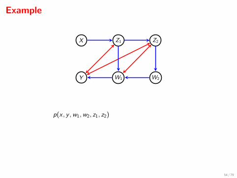
p(x , y ,w1,w2, z1, z2)
qyz1 (y , z1 | x ,w1) =qyw1z1z2 (y ,w1, z1 | x ,w2)
qyw1z1z2 (w1 | x ,w2)
and qyz1 (y | x ,w1) doesn’t depend upon x .
54 / 79
Example
Y W1 W2
X Z1
Z1
Z2
Z2
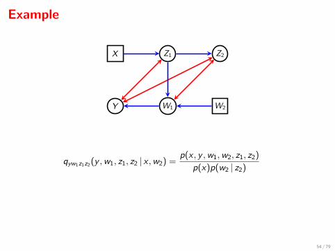
qyw1z1z2 (y ,w1, z1, z2 | x ,w2) =p(x , y ,w1,w2, z1, z2)
p(x)p(w2 | z2)
qyz1 (y , z1 | x ,w1) =qyw1z1z2 (y ,w1, z1 | x ,w2)
qyw1z1z2 (w1 | x ,w2)
and qyz1 (y | x ,w1) doesn’t depend upon x .
54 / 79

Example
Y W1 W2
X Z1
Z1 Z2
Z2
qyw1z1z2 (y ,w1, z1, z2 | x ,w2) =p(x , y ,w1,w2, z1, z2)
p(x)p(w2 | z2)
qyz1 (y , z1 | x ,w1) =qyw1z1z2 (y ,w1, z1 | x ,w2)
qyw1z1z2 (w1 | x ,w2)
and qyz1 (y | x ,w1) doesn’t depend upon x .
54 / 79

Example
Y W1 W2
X Z1
Z1 Z2
Z2
qyw1z1z2 (y ,w1, z1, z2 | x ,w2) =p(x , y ,w1,w2, z1, z2)
p(x)p(w2 | z2)
qyz1 (y , z1 | x ,w1) =qyw1z1z2 (y ,w1, z1 | x ,w2)
qyw1z1z2 (w1 | x ,w2)
and qyz1 (y | x ,w1) doesn’t depend upon x .
54 / 79

Example
Y W1 W2
X
Z1
Z1
Z2
Z2
qyw1z1z2 (y ,w1, z1, z2 | x ,w2) =p(x , y ,w1,w2, z1, z2)
p(x)p(w2 | z2)
qyz1 (y , z1 | x ,w1) =qyw1z1z2 (y ,w1, z1 | x ,w2)
qyw1z1z2 (w1 | x ,w2)
and qyz1 (y | x ,w1) doesn’t depend upon x .
54 / 79

Nested Markov ModelVarious equivalent formulations:
Factorization into Districts.For each reachable R in G,
qR(xR | xpa(R)\R) =∏
D∈D(G[R])
fD(xD∪pa(D))
some functions fD .
Weak Global Markov Property.For each reachable R in G,
A m-separated from B by C in G[R] =⇒ XA ⊥⊥ XB |XC [qR ].
Ordered Local Markov Property.For every intrinsic S and v maximal in S under some topological ordering,
Xv ⊥⊥ XV\mbG[S](v) |XmbG[S](v) [qS ].
Theorem. These are all equivalent.
55 / 79

Nested Markov ModelVarious equivalent formulations:
Factorization into Districts.For each reachable R in G,
qR(xR | xpa(R)\R) =∏
D∈D(G[R])
fD(xD∪pa(D))
some functions fD .
Weak Global Markov Property.For each reachable R in G,
A m-separated from B by C in G[R] =⇒ XA ⊥⊥ XB |XC [qR ].
Ordered Local Markov Property.For every intrinsic S and v maximal in S under some topological ordering,
Xv ⊥⊥ XV\mbG[S](v) |XmbG[S](v) [qS ].
Theorem. These are all equivalent.55 / 79
Outline
1 Motivation
2 Deriving constraints via fixing
3 The Nested Markov Model
4 Finer Factorizations
5 Discrete Parameterization
6 Testing and Fitting
7 Completeness
56 / 79

Heads and Tails
As established, we can factorize a graph into districts; however, finerfactorizations are possible.
1 2
3 4
In the graph above, there is a single district, but X1 ⊥⊥ X2.So could factorize this as
p(x1, x2, x3, x4) = p(x1, x2)p(x3, x4 | x1, x2)
= p(x1)p(x2)p(x3, x4 | x1, x2).
Note that the vertices {3, 4} can’t be d-separated from one another.
57 / 79

Heads and Tails
As established, we can factorize a graph into districts; however, finerfactorizations are possible.
1 2
3 4
In the graph above, there is a single district, but X1 ⊥⊥ X2.
So could factorize this as
p(x1, x2, x3, x4) = p(x1, x2)p(x3, x4 | x1, x2)
= p(x1)p(x2)p(x3, x4 | x1, x2).
Note that the vertices {3, 4} can’t be d-separated from one another.
57 / 79

Heads and Tails
As established, we can factorize a graph into districts; however, finerfactorizations are possible.
1 2
3 4
In the graph above, there is a single district, but X1 ⊥⊥ X2.So could factorize this as
p(x1, x2, x3, x4) = p(x1, x2)p(x3, x4 | x1, x2)
= p(x1)p(x2)p(x3, x4 | x1, x2).
Note that the vertices {3, 4} can’t be d-separated from one another.
57 / 79

Heads and Tails
As established, we can factorize a graph into districts; however, finerfactorizations are possible.
1 2
3 4
In the graph above, there is a single district, but X1 ⊥⊥ X2.So could factorize this as
p(x1, x2, x3, x4) = p(x1, x2)p(x3, x4 | x1, x2)
= p(x1)p(x2)p(x3, x4 | x1, x2).
Note that the vertices {3, 4} can’t be d-separated from one another.
57 / 79
Heads and Tails
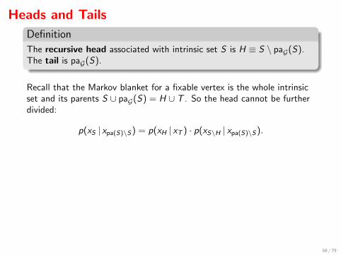
Definition
The recursive head associated with intrinsic set S is H ≡ S \ paG(S).The tail is paG(S).
Recall that the Markov blanket for a fixable vertex is the whole intrinsicset and its parents S ∪ paG(S) = H ∪ T . So the head cannot be furtherdivided:
p(xS | xpa(S)\S) = p(xH | xT ) · p(xS\H | xpa(S)\S).
1 2
3 4
But vertices in S \H may factorize:
p(x1, x2, x3, x4)
= p(x3, x4 | x1, x2)p(x1, x2)
= p(x3, x4 | x1, x2)p(x1)p(x2).
58 / 79
Heads and Tails
Definition
The recursive head associated with intrinsic set S is H ≡ S \ paG(S).The tail is paG(S).
Recall that the Markov blanket for a fixable vertex is the whole intrinsicset and its parents S ∪ paG(S) = H ∪ T . So the head cannot be furtherdivided:
p(xS | xpa(S)\S) = p(xH | xT ) · p(xS\H | xpa(S)\S).
1 2
3 4
But vertices in S \H may factorize:
p(x1, x2, x3, x4)
= p(x3, x4 | x1, x2)p(x1, x2)
= p(x3, x4 | x1, x2)p(x1)p(x2).
58 / 79
FactorizationsRecursively define a partition of reachable sets as follows. If R hasmultiple districts,
[R]G ≡ [D1]G ∪ · · · ∪ [Dk ]G ;
else R is intrinsic with head H, so
[R]G ≡ {H} ∪ [R \ H]G .
Theorem (Head Factorization Property)
p obeys the nested Markov property for G if and only if for everyreachable set R,
qR(xR | xpa(R)\R) =∏
H∈[R]G
qH(xH | xT ).
Here qH ≡ qS(H) is density associated with intrinsic set for H.(Recursive heads are in one-to-one correspondence with intrinsic sets.)
59 / 79

Heads and Tails
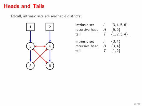
Recall, intrinsic sets are reachable districts:
1 2
3 4
5 6
intrinsic set I {3, 4, 5, 6}recursive head H {5, 6}tail T {1, 2, 3, 4}
intrinsic set I {3, 4}recursive head H {3, 4}tail T {1, 2}
So
[{3, 4, 5, 6}]G = {{3, 4}, {5, 6}}.
Factorization:
q3456(x3456 | x12) = q56(x56 | x1234) · q34(x34 | x12)
60 / 79

Heads and Tails
Recall, intrinsic sets are reachable districts:
1 2
3 4
5 6
intrinsic set I {3, 4, 5, 6}recursive head H {5, 6}tail T {1, 2, 3, 4}
intrinsic set I {3, 4}recursive head H {3, 4}tail T {1, 2}
So
[{3, 4, 5, 6}]G = {{3, 4}, {5, 6}}.
Factorization:
q3456(x3456 | x12) = q56(x56 | x1234) · q34(x34 | x12)
60 / 79

Heads and Tails
What if we fix 6 first?
1 2
3 4
5 6
intrinsic set I {3, 4, 5}recursive head H {4, 5}tail T {1, 2, 3}
intrinsic set I {3}recursive head H {3}tail T {1}
So
[{3, 4, 5}]G = {{3}, {4, 5}}.
Factorization:
q345(x345 | x12) = q45(x45 | x123) · q3(x3 | x1)
61 / 79

Heads and Tails
What if we fix 6 first?
1 2
3 4
5 6
intrinsic set I {3, 4, 5}recursive head H {4, 5}tail T {1, 2, 3}
intrinsic set I {3}recursive head H {3}tail T {1}
So
[{3, 4, 5}]G = {{3}, {4, 5}}.
Factorization:
q345(x345 | x12) = q45(x45 | x123) · q3(x3 | x1)
61 / 79

Heads and Tails
What if we fix 6 first?
1 2
3 4
5 6
intrinsic set I {3, 4, 5}recursive head H {4, 5}tail T {1, 2, 3}
intrinsic set I {3}recursive head H {3}tail T {1}
So
[{3, 4, 5}]G = {{3}, {4, 5}}.
Factorization:
q345(x345 | x12) = q45(x45 | x123) · q3(x3 | x1)
61 / 79

Heads and Tails
What if we fix 6 first?
1 2
3 4
5 6
intrinsic set I {3, 4, 5}recursive head H {4, 5}tail T {1, 2, 3}
intrinsic set I {3}recursive head H {3}tail T {1}
So
[{3, 4, 5}]G = {{3}, {4, 5}}.
Factorization:
q345(x345 | x12) = q45(x45 | x123) · q3(x3 | x1)
61 / 79
Heads and Tails
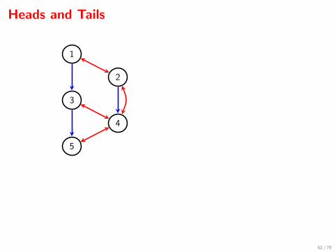
1
2
3
4
5
intrinsic set I {1, 2, 3, 4, 5}recursive head H {4, 5}tail T {1, 2, 3}
intrinsic set I {1, 2}recursive head H {1, 2}tail T ∅
intrinsic set I {3}recursive head H {3}tail T {1}
Factorization:
q12345(x12345) = q45(x45 | x123) · q3(x3 | x1) · q12(x12).
62 / 79

Heads and Tails
1
2
3
4
5
intrinsic set I {1, 2, 3, 4, 5}recursive head H {4, 5}tail T {1, 2, 3}
intrinsic set I {1, 2}recursive head H {1, 2}tail T ∅
intrinsic set I {3}recursive head H {3}tail T {1}
Factorization:
q12345(x12345) = q45(x45 | x123) · q3(x3 | x1) · q12(x12).
62 / 79

Heads and Tails
1
2
3
4
5
intrinsic set I {1, 2, 3, 4, 5}recursive head H {4, 5}tail T {1, 2, 3}
intrinsic set I {1, 2}recursive head H {1, 2}tail T ∅
intrinsic set I {3}recursive head H {3}tail T {1}
Factorization:
q12345(x12345) = q45(x45 | x123) · q3(x3 | x1) · q12(x12).
62 / 79

Heads and Tails
1
2
3
4
5
intrinsic set I {1, 2, 3, 4, 5}recursive head H {4, 5}tail T {1, 2, 3}
intrinsic set I {1, 2}recursive head H {1, 2}tail T ∅
intrinsic set I {3}recursive head H {3}tail T {1}
Factorization:
q12345(x12345) = q45(x45 | x123) · q3(x3 | x1) · q12(x12).
62 / 79

Outline
1 Motivation
2 Deriving constraints via fixing
3 The Nested Markov Model
4 Finer Factorizations
5 Discrete Parameterization
6 Testing and Fitting
7 Completeness
63 / 79
Parameterizations
Let M be a model (i.e. collection of probability distributions).
A parameterization is a continuous bijective map
θ :M→ Θ
with continuous inverse, where Θ is an open subset of Rd .
If θ, θ−1 are twice differentiable then this is a smooth parameterization.
We will assume all variables are binary; this extends easily to the generalcategorical / discrete case.
64 / 79

ParameterizationSay binary distribution p parameterized according to G if1
p(xV | xW ) =∑
O⊆C⊆V
(−1)|C\O|∏
H∈[C ]G
θH(xT ),
for some parameters θH(xT ) where O = {v : xv = 0}.
Note: there is no need to assume that θH(xT ) ∈ [0, 1], this comes for freeif p(xV | xW ) ≥ 0.
If suitable causal interpretation of model exists,
θH(xT ) = qS(0H | xT ) = p(0H | xS\H , do(xT\S))
6= p(0H | xT ).
Theorem (Evans and Richardson, 2015)
p is parameterized according to G if and only if it recursively factorizesaccording to G (so p ∈ N (G)).
1The definition of [·]G has to be extended to arbirary sets; see appendix.65 / 79
ParameterizationSay binary distribution p parameterized according to G if1
p(xV | xW ) =∑
O⊆C⊆V
(−1)|C\O|∏
H∈[C ]G
θH(xT ),
for some parameters θH(xT ) where O = {v : xv = 0}.Note: there is no need to assume that θH(xT ) ∈ [0, 1], this comes for freeif p(xV | xW ) ≥ 0.
If suitable causal interpretation of model exists,
θH(xT ) = qS(0H | xT ) = p(0H | xS\H , do(xT\S))
6= p(0H | xT ).
Theorem (Evans and Richardson, 2015)
p is parameterized according to G if and only if it recursively factorizesaccording to G (so p ∈ N (G)).
1The definition of [·]G has to be extended to arbirary sets; see appendix.65 / 79
Probabilities
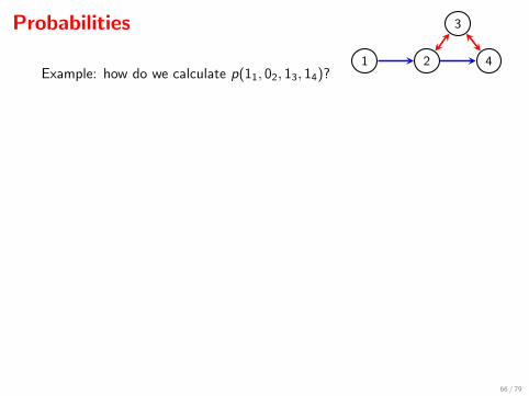
1 2 4
3
Example: how do we calculate p(11, 02, 13, 14)?
First,
p(11, 02, 13, 14) = q1(11) · q234(02, 13, 14 | 11).
Then q1(11) = 1− q1(01) = 1− θ1.
For the district {2, 3, 4} get
q234(02, 13, 14 | x1)
= q234(02 | x1)− q234(023 | x1)− q234(024 | x1) + q234(0234 | x1)
= θ2(x1)− θ23(x1)− θ2(x1)θ4(02) + θ2(x1)θ34(x1, 02).
Putting this all together:
p(11, 02, 13, 14)
= {1− θ1} {θ2(1)− θ23(1)− θ2(1)θ4(0) + θ2(1)θ34(1, 0)} .
66 / 79

Probabilities
1 2 4
3
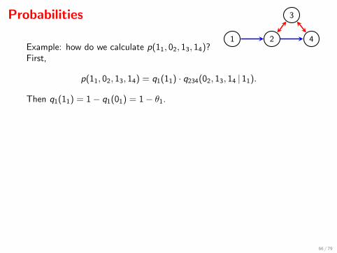
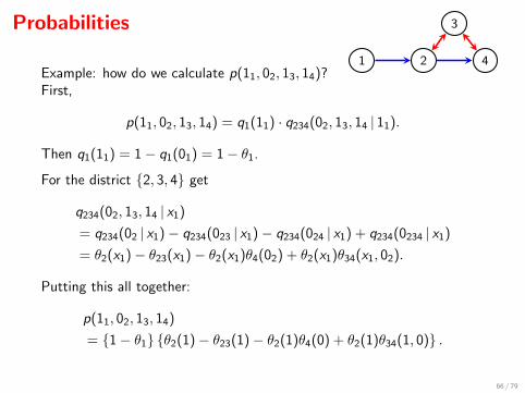
Example: how do we calculate p(11, 02, 13, 14)?First,
p(11, 02, 13, 14) = q1(11) · q234(02, 13, 14 | 11).
Then q1(11) = 1− q1(01) = 1− θ1.
For the district {2, 3, 4} get
q234(02, 13, 14 | x1)
= q234(02 | x1)− q234(023 | x1)− q234(024 | x1) + q234(0234 | x1)
= θ2(x1)− θ23(x1)− θ2(x1)θ4(02) + θ2(x1)θ34(x1, 02).
Putting this all together:
p(11, 02, 13, 14)
= {1− θ1} {θ2(1)− θ23(1)− θ2(1)θ4(0) + θ2(1)θ34(1, 0)} .
66 / 79
Probabilities
1 2 4
3
Example: how do we calculate p(11, 02, 13, 14)?First,
p(11, 02, 13, 14) = q1(11) · q234(02, 13, 14 | 11).
Then q1(11) = 1− q1(01) = 1− θ1.
For the district {2, 3, 4} get
q234(02, 13, 14 | x1)
= q234(02 | x1)− q234(023 | x1)− q234(024 | x1) + q234(0234 | x1)
= θ2(x1)− θ23(x1)− θ2(x1)θ4(02) + θ2(x1)θ34(x1, 02).
Putting this all together:
p(11, 02, 13, 14)
= {1− θ1} {θ2(1)− θ23(1)− θ2(1)θ4(0) + θ2(1)θ34(1, 0)} .
66 / 79

Example 1
Z X Y
Intrinsic Sets Z X ,Y X
Heads Z Y XTails ∅ Z ,X Z
So parameterization is just
p(z = 0), p(x = 0 | z) p(y = 0 | x , z).
Model is saturated.
67 / 79

Example 1
Z X Y
Intrinsic Sets Z X ,Y XHeads Z Y X
Tails ∅ Z ,X Z
So parameterization is just
p(z = 0), p(x = 0 | z) p(y = 0 | x , z).
Model is saturated.
67 / 79

Example 1
Z X Y
Intrinsic Sets Z X ,Y XHeads Z Y XTails ∅ Z ,X Z
So parameterization is just
p(z = 0), p(x = 0 | z) p(y = 0 | x , z).
Model is saturated.
67 / 79

Example 1
Z X Y
Intrinsic Sets Z X ,Y XHeads Z Y XTails ∅ Z ,X Z
So parameterization is just
p(z = 0), p(x = 0 | z) p(y = 0 | x , z).
Model is saturated.
67 / 79

Example 2
10 2 3 4
p(00, 11, 12, 03, 04) = p(00, 11, 12, 03) · q4(04 | 00, 11, 12, 03)
p(00, 11, 12, 03) = q2(12 | 11) · q013(00, 11, 03 | 12)
q013(00, 11, 03 | 12) = q03(00, 03 | 12)− q013(00, 01, 03 | 12)
= θ03(1)− θ013(1)
so
p(00, 11, 12, 03, 04) = {1− θ2(1)} {θ03(1)− θ013(1)} · θ4(0, 1, 1, 0).
68 / 79

Example 2
10 2 3
4
p(00, 11, 12, 03, 04) = p(00, 11, 12, 03) · q4(04 | 00, 11, 12, 03)
p(00, 11, 12, 03) = q2(12 | 11) · q013(00, 11, 03 | 12)
q013(00, 11, 03 | 12) = q03(00, 03 | 12)− q013(00, 01, 03 | 12)
= θ03(1)− θ013(1)
so
p(00, 11, 12, 03, 04) = {1− θ2(1)} {θ03(1)− θ013(1)} · θ4(0, 1, 1, 0).
68 / 79

Example 2
10 2 3 4
p(00, 11, 12, 03, 04) = p(00, 11, 12, 03) · q4(04 | 00, 11, 12, 03)
p(00, 11, 12, 03) = q2(12 | 11) · q013(00, 11, 03 | 12)
q013(00, 11, 03 | 12) = q03(00, 03 | 12)− q013(00, 01, 03 | 12)
= θ03(1)− θ013(1)
so
p(00, 11, 12, 03, 04) = {1− θ2(1)} {θ03(1)− θ013(1)} · θ4(0, 1, 1, 0).
68 / 79
Motivation
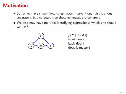
So far we have shown how to estimate interventional distributionsseparately, but no guarantee these estimates are coherent.
We also may have multiple identifying expressions: which one shouldwe use?
X M Y
L p(Y | do(X ))front door?back door?does it matter?
We can test constraints separately, but ultimately don’t have a wayto check if the model is a good one.
Being able to evaluate a likelihood would allow lots of standardinference techniques (e.g. LR, Bayesian).
Even better, if model can be shown smooth we get nice asymptoticsfor free.
All this suggests we should define a model which we can parameterize.
69 / 79

Motivation
So far we have shown how to estimate interventional distributionsseparately, but no guarantee these estimates are coherent.
We also may have multiple identifying expressions: which one shouldwe use?
X M Y
L p(Y | do(X ))front door?back door?does it matter?
We can test constraints separately, but ultimately don’t have a wayto check if the model is a good one.
Being able to evaluate a likelihood would allow lots of standardinference techniques (e.g. LR, Bayesian).
Even better, if model can be shown smooth we get nice asymptoticsfor free.
All this suggests we should define a model which we can parameterize.
69 / 79

Outline
1 Motivation
2 Deriving constraints via fixing
3 The Nested Markov Model
4 Finer Factorizations
5 Discrete Parameterization
6 Testing and Fitting
7 Completeness
70 / 79

Exponential Families
Theorem
Let N (G) be the collection of binary distributions that recursivelyfactorize according to G. Then N (G) is a curved exponential family ofdimension
d(G) =∑
H∈H(G)
2| tail(H)|.
(This extends in the obvious way to finite discrete distributions.)
This justifies classical statistical theory:
likelihood ratio tests have asymptotic χ2-distribution;
BIC as Laplace approximation of marginal likelihood.
(Shpitser et al., 2013) give an alternative log-linear parametrization.
71 / 79

Algorithms for Model Search
Can, for example, use greedy edge replacement for a score-basedapproach (Evans and Richardson, 2010).
Shpitser et al. (2011) developed efficient algorithms for evaluatingprobabilities in the alternating sum.
Currently no equivalent of PC algorithm for full nested model.
Can use FCI algorithm (Spirtes at al., 2000) for ordinary Markovmodels associated with ADMG (conditional independences only), ingeneral this is a supermodel of the nested model (see Evans andRichardson, 2014).
Open Problems:
Nested Markov equivalence;
Constraint based search;
Gaussian parametrization.
72 / 79
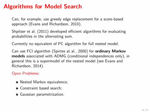
Outline
1 Motivation
2 Deriving constraints via fixing
3 The Nested Markov Model
4 Finer Factorizations
5 Discrete Parameterization
6 Testing and Fitting
7 Completeness
73 / 79

Completeness
Could the nested Markov property be further refined?
No and Yes.
Theorem (Evans, 2015)
The constraints implied by the nested Markov model are algebraicallyequivalent to causal model with latent variables (with suff. large latentstate-space).
‘Algebraically equivalent’ = ‘of the same dimension’.
So if the latent variable model is correct2, fitting the nested model isasymptotically equivalent fitting the LV model.
However, there are additional inequality constraints. e.g. Instrumentalinequalities, CHSH inequalities etc.,
Potentially unsatisfactory as may not be a causal model corresponding toour inferred parameters.
2and we are in the relative interior of the model space.74 / 79

Completeness
Could the nested Markov property be further refined? No and Yes.
Theorem (Evans, 2015)
The constraints implied by the nested Markov model are algebraicallyequivalent to causal model with latent variables (with suff. large latentstate-space).
‘Algebraically equivalent’ = ‘of the same dimension’.
So if the latent variable model is correct2, fitting the nested model isasymptotically equivalent fitting the LV model.
However, there are additional inequality constraints. e.g. Instrumentalinequalities, CHSH inequalities etc.,
Potentially unsatisfactory as may not be a causal model corresponding toour inferred parameters.
2and we are in the relative interior of the model space.74 / 79
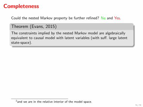
Completeness
Could the nested Markov property be further refined? No and Yes.
Theorem (Evans, 2015)
The constraints implied by the nested Markov model are algebraicallyequivalent to causal model with latent variables (with suff. large latentstate-space).
‘Algebraically equivalent’ = ‘of the same dimension’.
So if the latent variable model is correct2, fitting the nested model isasymptotically equivalent fitting the LV model.
However, there are additional inequality constraints. e.g. Instrumentalinequalities, CHSH inequalities etc.,
Potentially unsatisfactory as may not be a causal model corresponding toour inferred parameters.
2and we are in the relative interior of the model space.74 / 79

Big Picture
M
N
O
all distributions
75 / 79

Big Picture
M
N
O
all distributions
75 / 79

Big Picture
M
N
O
all distributions
75 / 79

Big Picture
M
N
O
all distributions
75 / 79

More on the nested Markov model
Evans (2015) shows that the nested Markov model implies allalgebraic constraints arising from the corresponding DAG with latentvariables;
A parameterization for discrete variables is given by Evans + R(2015), via an extension of the Mobius parametrization;
In general a latent DAG model may also imply inequalities notcaptured by the nested Markov model: cf. the CHSH / Bellinequalities in quantum mechanics;
The nested model may also be defined by constraints resulting froman algorithm given in (Tian, 2002b).
Future Work
Characterizing nested Markov equivalence;
Methods for inferring graph structure.
76 / 79
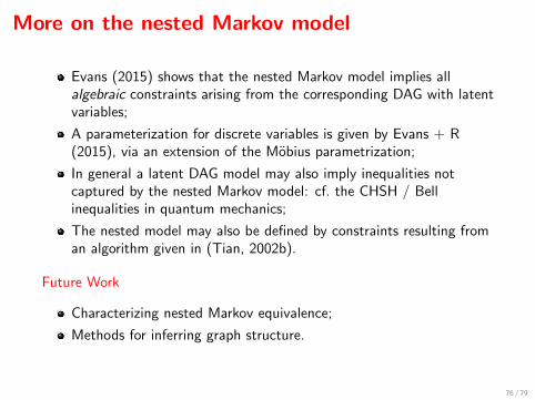

Nested Markov model references
Evans, R. J. (2015). Margins of discrete Bayesian networks. arXiv preprint:1501.02103.
Evans, R. J. and Richardson, T. S. (2015). Smooth, identifiable supermodels of discreteDAG models with latent variables. arXiv:1511.06813.
Evans, R.J. and Richardson, T.S. (2014). Markovian acyclic directed mixed graphs fordiscrete data. Annals of Statistics vol. 42, No. 4, 1452-1482.
Richardson, T.S., Evans, R. J., Robins, J. M. and Shpitser, I. (2017). Nested Markovproperties for acyclic directed mixed graphs. arXiv:1701.06686.
Richardson, T.S. (2003). Markov Properties for Acyclic Directed Mixed Graphs. TheScandinavian Journal of Statistics, March 2003, vol. 30, no. 1, pp. 145-157(13).
Shpitser, I., Evans, R.J., Richardson, T.S., Robins, J.M. (2014). Introduction to NestedMarkov models. Behaviormetrika, vol. 41, No.1, 2014, 3–39.
Shpitser, I., Richardson, T.S. and Robins, J.M. (2011). An efficient algorithm for computinginterventional distributions in latent variable causal models. In Proceedings of UAI-11.
Shpitser, I. and Pearl, J. (2006). Identification of joint interventional distributions inrecursive semi-Markovian causal models. Twenty-First National Conference on ArtificialIntelligence.
Tian, J. (2002) Studies in Causal Reasoning and Learning, CS PhD Thesis, UCLA.
Tian, J. and Pearl, J. (2002a). A general identification condition for causal effects. InProceedings of AAAI-02.
Tian, J. and J. Pearl (2002b). On the testable implications of causal models with hiddenvariables. In Proceedings of UAI-02.
77 / 79

Parameterization References
(Including earlier work on the ordinary Markov model.)
Evans, R.J. and Richardson, T.S. – Maximum likelihood fitting of acyclic directed mixedgraphs to binary data. UAI, 2010.
Evans, R.J. and Richardson, T.S. – Markovian acyclic directed mixed graphs for discretedata. Annals of Statistics, 2014.
Shpitser, I., Richardson, T.S. and Robins, J.M. An efficient algorithm for computinginterventional distributions in latent variable causal models. UAI, 2011.
Shpitser, I., Richardson, T.S., Robins, J.M. and Evans, R.J. – Parameter and structurelearning in nested Markov models. UAI, 2012.
Shpitser, I., Evans, R.J., Richardson, T.S. and Robins, J.M. – Sparse nested Markov modelswith log-linear parameters. UAI, 2013.
Shpitser, I., Evans, R.J., Richardson, T.S. and Robins, J.M. – Introduction to NestedMarkov Models. Behaviormetrika, 2014.
Spirtes, P., Glymour, G., Scheines, R. – Causation Prediction and Search, 2nd Edition, MITPress, 2000.
78 / 79

Inequality References
Bonet, B. – Instrumentality tests revisited, UAI, 2001.
Cai Z., Kuroki, M., Pearl, J. and Tian, J. – Bounds on direct effects in the presence ofconfounded intermediate variables, Biometrics, 64(3):695–701, 2008.
Evans, R.J. – Graphical methods for inequality constraints in marginalized DAGs, MLSP,2012.
Evans, R.J. – Margins of discrete Bayesian networks, arXiv:1501.02103, 2015.
Kang, C. and Tian, J. – Inequality Constraints in Causal Models with Hidden Variables,UAI, 2006.
Pearl, J. – On the testability of causal models with latent and instrumental variables, UAI,1995.
79 / 79

Partition Function for General Sets
Let I(G) be the intrinsic sets of G. Define a partial ordering ≺ on I(G)by S1 ≺ S2 if and only if S1 ⊂ S2. This induces an isomorphic partialordering on the corresponding recursive heads.
For any B ⊆ V let
ΦG(B) = {H ⊆ B |H maximal under ≺ among heads contained in B};
φG(B) =⋃
H∈ΦG(B)
H.
So ΦG(B) is the ‘maximal heads’ in B, φG(B) is their union.
Define (recursively)
[∅]G ≡ ∅[B]G ≡ ΦG(B) ∪ [φG(B)]G .
Then [B]G is a partition of B.
80 / 79

d-Separation
A path is a sequence of edges in the graph; vertices may not be repeated.
A path from v to w is blocked by C ⊆ V \ {v ,w} if either
(i) any non-collider is in C :
c c
(ii) or any collider is not in C , nor has descendants in C :
d d
e
Two vertices v and w are d-separated given C ⊆ V \ {v ,w} if all pathsare blocked.
81 / 79
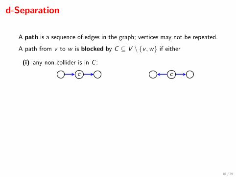
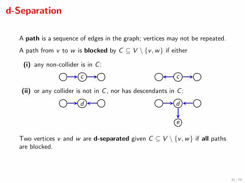

The IV Model
Assume four variable DAG shown, but U unobserved.
Z X Y
U
Marginalized DAG model
p(z , x , y) =
∫p(u) p(z) p(x | z , u) p(y | x , u) du
Assume all observed variables are discrete; no assumption made aboutlatent variables.
Nested Markov property gives saturated model, so true model of fulldimension.
82 / 79

The IV Model
Assume four variable DAG shown, but U unobserved.
Z X Y
Marginalized DAG model
p(z , x , y) =
∫p(u) p(z) p(x | z , u) p(y | x , u) du
Assume all observed variables are discrete; no assumption made aboutlatent variables.
Nested Markov property gives saturated model, so true model of fulldimension.
82 / 79

Instrumental Inequalities
Z X
U
YThe assumption Z 6→ Y is important.Can we check it?
Pearl (1995) showed that if the observed variables are discrete,
maxx
∑y
maxz
P(X = x ,Y = y |Z = z) ≤ 1. (∗)
This is the instrumental inequality, and can be empirically tested.
If Z ,X ,Y are binary, then (∗) defines the marginalized DAG model(Bonet, 2001). e.g.
P(X = x ,Y = 0 |Z = 0) + P(X = x ,Y = 1 |Z = 1) ≤ 1
83 / 79
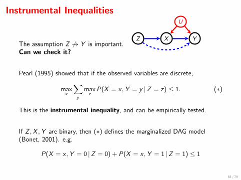