Part I

Network Analyzer and NetworkAnalysis1 Objectives

Upon completion of the lab experiment , the student will become familiarwith the followingtopics:

1. Get acquainted with the major elements of the Network Analyzer.

2. Using the Network Analyzer to characterize two port passive elements,such as lters, coaxial cable etc.

3. Understand the meaning of S parameter measurement using a NetworkAnalyzer.

4. Get familiar with the various Reection and Transmission parameterssuch as return loss, reection coe¢ cient, time delay, and group delay.

5. Understand the basic properties of passive networks, such as lossless,reciprocal etc.

6. Understand the concept of various calibration of the Network Analyzer.

2 Prelab Exercise

1. Dene the following parameters: return loss, lossless network, unitarymatrix, delay, phase delay, group delay.

2. An electromagnetic wave s (t) = 2109t pass through 10m coaxial cable,the velocity of the electromagnetic wave is 2=3c;

(a) Find the dielectric constant of the coaxial cable.

(b) Calculate the time delay of the cable.

1

(c) Calculate the phase delay of the cable..

3. Two set of measurement were taken, at frequencies f1 and f2, can youdecide if either is dispersive?

Frequency jH (f)j (dB) 6 H (f) (deg)f1 0 102f1 0 403f1 0 704f1 0 100

Frequency jH (f)j (dB) 6 H (f) (deg)f2 0 102f2 0 403f2 0 1004f2 0 190

1. The measurement results of 4 ports network, directional coupler is givenby the scattering matrix,

[S] =

0BBB@0 1p

21p2j 0

1p2

0 0 1p2j

1p2j 0 0 1p

2

0 1p2j 1p

20

1CCCAdetermine whether the network is matched, reciprocal, and lossless?

2.1 References

[1] D.M. Pozar, Microwave engineering, 3rd edition, 2005 John-Wiley&Sons.

3 Background Theory

3.1 Transmission Line Summary

Transmission line theory apply, when the dimension of the line is in the sameorder of magnitude as the wavelength transmitted through. In this case ifthe load impedance ZL 6= Z0; part of the incident wave is reected back to

2

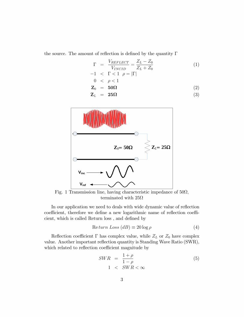
the source. The amount of reection is dened by the quantity

=VREFLECTVINCID

=ZL Z0ZL + Z0

(1)

1 < < 1 = jj0 < < 1

Z0 = 50 (2)

ZL = 25 (3)

Z0= 50I ZL= 25I

Vinc

Vref

Fig. 1 Transmission line, having characteristic impedance of 50;terminated with 25

In our application we need to deals with wide dynamic value of reectioncoe¢ cient, therefore we dene a new logarithmic name of reection coe¢ -cient, which is called Return loss , and dened by

Re turn Loss (dB) 20 log (4)

Reection coe¢ cient has complex value, while ZL or Z0 have complexvalue. Another important reection quantity is StandingWave Ratio (SWR),which related to reection coe¢ cient magnitude by

SWR =1 +

1 (5)

1 < SWR <1

3

3.2 Propagation Constant

Propagation constant is a complex quantity, which describe the e¤ect of thetransmission line, on the propagate wave. The linear e¤ects describe by thereal part, the attenuation (neper=meter) ; and imaginary part (radian=meter),phase constant , or wave number and dened by

= + j (6)

=2

3.3 Network Analyzer

RefR1

RefR2

A B

LO

RFSource

RFswitch

Splitter Splitter

Dire

ctio

nal

Cou

pler

Dire

ctio

nal

Cou

pler

Testport 1

Testport 2

3 dBAttenuator

ReceiverReceiver

TransmitedReflectedTransmited

Reflected

Incidentpower

DUT

Fig. 2 Major elements of Network Analyzer

3.4 Signal Source

The signal source supplies the stimulus for our stimulus-response test sys-tem. We can either sweep the frequency of the source or sweep its power

4

level. Modern source are synthesized sources, providing excellent frequencyresolution and stability.

3.4.1 Signal Separation Devices- Splitter and Directional Coupler.

The next major area is the signal separation block. The hardware used forthis function is generally called the test set. There are two functions thatoursignal-separation hardware must provide. The rst is to measure a portion

of the incident signal to provide a reference for ratioing. This can be donewith splitters or directional couplers. Splitters are usually resistive. Theyare non-directional devices and can be very broadband. The trade-o¤ is thatthey usually have 6 dB or more of loss in each arm. Directional couplershave very low insertion loss (through the main arm) and good isolation anddirectivity.The second function of the signal splitting hardware is to separate the

incident (forward) and reected (reverse) traveling waves at the input of ourDUT.

3.4.2 Receiver

The receiver provides the means of converting and detecting the RF or mi-crowave signals to a lower IF. The tuned receivers provide a narrowband-passIntermediate-Frequency (IF ) lter to reject spurious signals and minimizedthe noise oor of the receiver. The vector measurement systems have the highdynamic range, and immunity to harmonic and spurious responses, they canmeasure phase relationships of input signals and provide the ability to makecomplex calibrations that lead to more accurate measurements.

4 Input Impedance Zin and Characteristic Im-pedance Z0

According to the transmission line theory input impedance of a lossless trans-mission line terminated by load ZL; expressed by

Zin = Z0ZL + jZ0 tan l

Z0 + jZL tan l(7)

where Z0 is characteristic impedance and l is the line length:

5

Z0

l

Zin ZLβ

Fig-3 Input impedance of transmission line with arbitrary load ZL:

If ZL = 0 or ,ZL =1 equation [7] reduce to

Zin(sc) = jZ0 tan l (8)

Zin(oc) =Z0jcot l

using equation [8] we may rewrite

Z0 =pZin(sc)Zin(oc) (9)

The idea of equation [9] is a useful way to measure characteristic impedance,of DUT, by measuring Zin(sc) and Zin(oc) of the DUT.

5 The Denition of S-Parameter

Scatter Parameters, also called S-parameters. Like the H,Y,Z or ABCD pa-rameter, they describe the performance of linear n-ports device completely.They relate to the traveling waves that are scattered or reected when a net-work is inserted into a transmission line of a certain characteristic impedanceZL.

Incient wave a1

Reflected wave b1

LTINetwork1 2

Incient wave a2

Reflected wave b2

S22S11

S21

S12

6

Fig. 4 S parameter ow graph

S-parameters are important in microwave design because they are easierto measure and to work with at high frequencies than other kinds of twoport parameters. However, it must kept in mind that -like all other twoport parameters, S-parameters apply to LTI network, I.e. they represent thelinear behavior of the two ports.S-parameters are dened as:

b1 = S11a1 + S12a2 (10)

b2 = S21a1 + S22a2

ai -E¤ective value (rms) of the incident wave traveling towards the ithtwo port gate.

bi -E¤ective value (rms) of the wave reected back from the i th twoport gate.

The signal ow graph gives the situation for the S-parameter interpreta-tion in voltages:Looking at the S parameter coe¢ cients individually, we have

S11 = 1 =b1a1=Vreected at port 1Vforward port 1

a2=0

(11)

S12 =b1a2=Vout of port 1Vforward port 2

a1=0

S21 =b2a1=

Vout of port 2Vforward port 1

a2=0

S22 = 2 =b2a2=Vout of port 2Vforward port 2

a1=0

S11 and S21 are determined by measuring the magnitude and phase of theincident, reected and transmitted signals when the output is terminated ina perfect Z0 load. This condition guarantees that a2 is zero. S11 is equivalentto the input complex reection coe¢ cient or impedance of the DUT, and S21is the forward complex transmission coe¢ cient.

7

Likewise, by placing the source at port 2 and terminating port 1 in aperfect load (making a a1 zero), S22 and S12 measurements can be made. S22is equivalent to the output complex reection coe¢ cient or output impedanceof the DUT, and S12 is the reverse complex transmission coe¢ cient.

5.1 Properties of Network

Matched network S11 = S22 = 0

A reciprocal network -S-parameter matrix is symmetric about itsdiagonal or equal to its transpose, Sij = Sji

Lossless network the power incident on the network must be equal

to the power reected, ornXi=1

jaij2 =nXi=1

jbij2 ; or in in mathematics, a

unitary matrix is an n by n complex matrix U satisfying the conditionU+U = UU+ = In:

5.2 Nondispersive (Distortionless) Transmission

In communication systems, a nondispersive channel, or low distortion is oftendesired. This implies that the channel output y(t) is just proportional to atime delayed version of the input x (t)

y(t) = Ax(t Td) (12)

R

Cx(t) y(t)

Fig-5 An arbitrary network

where A is the gain (which may be less than unity) and Td is the delay.

8

5.2.1 Delay and Phase Delay

For a non-dispersive DUT, e.g. a coaxial cable, phase (f) is a linear functionof frequency:

(f) = 360fTd (13)

where Td is the delay time of the cable which is the time that the electro-magnetic wave pass through the cable. Phase delay is directly related to itsmechanical length l via the permittivity r of the dielectric material withinthe cable, therefore the time delay is dened by

Td =lprc

(14)

The corresponding requirement in the frequency domain is obtained bytaking the Fourier transform of both sides of Eq. (12).

Y (f) = AX(f) exp (j2fTd) (15)

Thus, for distortionless transmission, we require that the transfer functionof the channel be given by

H(f) =Y (f)

X(f)= A exp (j2jfTd) (16)

which implies that, distortionless network, must be satised two require-ments:

1. The amplitude response versus frequency must be at. That is

H(f) = constamt = A (17)

2. The phase response is a linear function of frequency. That is

(f) = 6 H(f) = 2fTd (18)

When the rst condition is satised, there is no amplitude distortion.When the second condition is satised, there is no phase distortion. Fornon dispersive transmission, both conditions must be satised.

9

By Eq:(14), it is required that Td (f) = constant for non dispersive trans-mission. If Td (f) is not constant, there is phase distortion. The linearity ofphase versus frequency is characterized by group delay which dened as

(f) 1

360

d (f)

df(19)

That is the negative of the rate of change of phase ( which measurein degree) with frequency. The quantity has the dimension of time, butthe question is; what time does it represent? Many textbooks follow thedenition of group delay with a discussion of an ideal element that delays asignal by time Td:

10

Part II

Experiment Procedure6 Required Equipment

1. RF Network Analyzer E5062A

2. Type N calibir4ation kit Agilent - 85032E

3. Band Pass Filter Mini - Circuit BBP - 10.7 MHz

4. Terminator 50 NTRM - 50

5. Agilent ADS simulation software

6.1 Simulating a Network Analyzer Measurement.

In this part of the experiment we simulate the reection and transmissionmeasurement of a 10.7MHz BPF.

1. Simulate a reection and transmission measurement (S11 and S21) ; ofa 10.7 MHz BPF , using ADS software. The denition of the lterparameter is ginen in Fig. 10.

Fig. 9 simulation of reection and transmission of 10.7MHz BPF

11

2 4 6 8 10 12 14 16 180 20

-30

-10

-50

0

freq, MHz

dB(S

(2,1

))

Passband ripple-3dB point

BW pass

Ast

op

BWstop

Fig.-10 Denition of an Elliptic BPF

2. Draw a graph of S11 (magnitude), S11 (dB), S21 and and Fill Table-1according to simulation results.

BPF Electrical Transmission ResultsPassband IL Stopband

Center Freq. BW(-3dB) IL > 20dB@Freq. IL@7.5 MHz IL@15 MHz

Selectivity20dB bandwidth3dB bandwidth

Reection

max jj 9 to 12MHz; max RL 9 to 12MHz jj@7:5 RL@15MHz

Table-1

12

7 Getting Started With Network Analyzer

7.1 Front Panel View Refer to Fig.-6:

1. Standby Switch

Allows the switch between power-on (j) and standby mode (Ö) on theE5061A/E5062A.

2. LCD Screen

Displays measurement traces, instrument setting conditions, and menubars.

3. ACTIVE CH/TRACE Block

A group of keys used for selecting the active channel and an activetrace.

4. RESPONSE Block

A group of keys used for the selection of a measurement parame-ters/data formats, displaying, calibration, etc.

5. STIMULUS Block

A group of keys used for specifying the setup for signal sources, trigger,etc.

13

RFIN

RFOUT

1 2 643

7

12 11 10

8

95

Fig-6 Front panel tour

6. NAVIGATION Block

A group of keys used for the movement/selection of the focus in menubars/soft-key menu bar/dialog boxes and for manipulating markers.

7. ENTRY Block

A group of keys used for entering numeric data on the E5061A/E5062Asettings.

8. INSTR STATE Block

A group of keys used for specifying the setup for controlling and man-aging the E5061A/E5062A such as executing printing measurementresults, and presetting (initializing) the E5061A/E5062A.

9. MKR/ANALYSIS Block

A group of keys used for analyzing measurement results through mark-ers, the limit test function, etc.

10. Test Port

14

While the signal is being output from a test port, the yellow LED abovethe test port lights up. The connector type adopted is the 50 -basedN-type (female) connector.

11. Front USB Port

Used to connect a printer, or an ECal module compatible with the USB(Universal Serial Bus). Using a USB port allows the accessories to beconnected after the E5061A/E5062A has been powered on.

12. Ground Terminal

Connected to the chassis of the E5061A/E5062A. You can connect abanana type plug to this terminal

8 Reection Measurement

8.1 Preparation to Reection Measurements, Reec-tion Calibration

When you require best possible accuracy, or you need to add an adaptor orcable between the DUT and the test port, it is strongly recommended toperform a proper calibration.

1. Press Preset and OK .

2. Press CAL key and then choose Calibrate, 1- Port Cal

3. Connect an open to the reection port and press Open(f) (see gure7).

4. Connect a short to the reection port and press Short(f).

5. Connect a load to the reection port and press Load and in the endpress Done.

6. You use 3 standards, (open short and 50 load); could you determineZ0 using two standards? Prove your answer using proper equation.

7. Disconnect the load (50 termination) and return all the standardsdevices carefully to their box.

15

RFIN

RFOUT

50ΩLoad

open

short

Fig. 7 Calibration for Reection measurement

8.2 Preparation to Reection Measurement, SettingSignal Source

S. parameters is a ratioing measurement. If your device is sensitive to theincident power, you can increase or decrease the incident power.

1. Connect a 10.7MHz BPF to the Network Analyzer as shown in Figure8.

2. Press the Preset key situated at INSTR STATE Block.

3. Press theMeasr key situated at Response Block, and choose S11 fromthe soft menu, and press Enter.

4. Press the Scale key, and choose Autoscale from the soft menu.

5. At the STIMULUS Block press: Start key and insert 5 MHz bypressing 5 M=, press Stop key and insert 20 MHz.

16

RFIN

RFOUT

10.7

MH

zBP

F

50ΩLoad

Fig. 8 Basic reection neasurement

6. By default the power level of the Network Analyzer is 0 dBm (1mw). Ifnecessary you can change the power by pressing Sweep Setup keys andthen choose Power option and set power level to 3dBm, by pressing 31 keys.

9 Reection Measurement of a BPF

Under Reection measurement you can measure: reection coe¢ cient mag-nitude and phase, return loss , SWR, and impedance of a DUT.

1. Press the Preset key situated at INSTR STATE Block.

2. Press theMeasr key situated at Response Block, and choose S11 fromthe soft menu, and press Enter.

3. Press the Scale key, and choose Autoscale from the soft menu.

4. Press Freq, then Start 1 MHz and Stop 25 MHz, Scale, Autoscale,return loss (S11; reection coe¢ cient jj in dB) as a function of fre-quency is displayed). Save the data of S11 and S22 on magneticmedia, Excell and image format.

17

5. Press Format, Lin Mag, to get the absolute value of reection co-e¢ cient as a function of frequency is displayed ( = jj):Set marker1 to 10.7MHz, and marker 2 to 25MHz. Explain what happen to theincident power at that frequencies? Save the data on magneticmedia.

6. Press Format Polar, to get polar plot of the reection coe¢ cient,could you explain where ; 6 and frequency is displayed?.Save thedata on magnetic media.

7. Fill Table-2.

Freq(MHz). RL(data) RL(meas.) jj(meas.) Pinc (mw) Pref = jj2 PincStop band x x x x x

5.3 -0.2 115 -0.4 1

10.7 (center) -17.6 1Table-2

9.1 Standing Wave Ratio and Impedance

1. Press Format, and SWR. The SWR as a function of frequency isdisplayed.Save the data on magnetic media.

2. Press Format and Smith Chart for getting a display of the real andimaginary values of the impedance as function of frequency. Set thestart frequency to 7 MHz and stop frequency 20 MHz, verify that theimpedance of the lter is about 50 in the pass Band (8:5 to 12:5MHz).Savethe data on magnetic media.

3. Fill Table-3

Stop band<7.5MHzSWR(Data ) SWR(measured)

16Pass band(9.5 to 11.5MHz)

SWR(Data ) SWR(measured)< 1:7

Table-3

18

10 Make a Transmission Measurement of aBPF

In this part of the experiment you measure insertion loss (attenuation, S21)of a BPF as a function of frequency using Transmission measurement.

10.1 Preparation to transmission Measurement- Re-sponse Calibration

In this part of the experiment we eliminate the errors due to frequency re-sponse of the external cable connected between port-1 and port-2 of theNetwork Analyzer.

1. Connect a coax cable to the network between RF out port and RF inport (see Fig. 10 dashed line).

2. Set the frequencies range, 300kHz to 1GHz.

3. Press Preset, Ok andMeasurement, S21.

4. Press CAL, calibrate, Response(Thru), Thru, Done.

10.2 Transmission Measurement of an Elliptic BPF.

In this part you measure the insertion loss of the BPF, at the pass bandand at the stop band.

1. Disconnect the coaxial cable and connect the BPF to the reection portof the Network Analyzer, as indicated in Figure 10.

2. Set the frequency range to start frequency 5MHz stop frequency 20MHz,transmission coe¢ cient measurement in dB is displayed (S21) .

3. Press Scale, Autoscale. and Save the data of S21 and S12 on yourmedia, Excell, and image format.

4. Press Marker Search, Max verify that the center frequency of thelter is about 10.7 MHz and ll Table-4.

19

5. Set the marker to 9.5 MHz and 11.5 MHz by pressing Marker 9.5MHz , and then 11.5 MHz, verify that the insertion loss is less than1.5 dB.

Pass Band measurementsCenter Freq. Passband(IL<1.5dB) Typ. bandwidth(-3dB) Bandwidth(-20dB)(10:7MHz) (9:5 to 11:5MHz) (8:9 12:7MHz) (7:8 14:4)

Selectivity20dB3dB

IL@9.5 MHz IL@11.5 MHz IL@Center Freq

(1:7) (1dB) (1dB)

Stop BandIL@7.5 MHz IL@15 MHz IL@0.6 MHz Freq.@-20dB(30dB) (30dB) (60dB) (7:6&14:4)

Table-4

6. Measure the phase of the lter in the pass band (9.5-11.5 MHz), ex-plain if the phase is linear in the passband?

RFIN

RFOUT

10.7

MH

zB

PF Responsecalibration

Filter transmissionmeasurement

Fig. 10 Response calibration and transmission measurement of a BPF.

20

11 Delay and Phase Delay

In this part of the experiment you simulate and measure the delay (groupdelay), and phase delay of a coaxial cable.

11.1 Group Delay, and Phase Simulation

1. Simulate a 5m coaxial cable as indicated in Fig. 11

2. Allow group delay simulation by double click on S PARAMETER,then click on parameters, and select Group delay.

S_ParamSP1

Step=10.0 kHzStop=200 MHzStart=1.0 MHz

S-PARAMETERS

COAXTL1

Rho=1TanD=0.002Er=2.1L=5000 mmDo=3.275 mmDi=0.9 mm

P_1TonePORT1

Freq=1 GHzP=polar(dbmtow(0),0)Z=50 OhmNum=1

TermTerm2

Z=50 OhmNum=2

Fig-11 Group delav and phase delay simulation

3. Plot a graph of delay S21 (group delay) as a function of frequency,according to the graph explain if the cable is dispersive element?

4. Calculate, phase constant ;and phase delay at 100MHz. Plot a graphof S21 phase and nd the phase delay at 100 MHz, you can verify yourresult by changing the graph expression to plot_vs(unwrap(phase(S(2,1))),freq).

5. Replace the coaxial cable with elliptic band pass lter as indicated inFig. 12 and simulate the group delay of the lter.

21

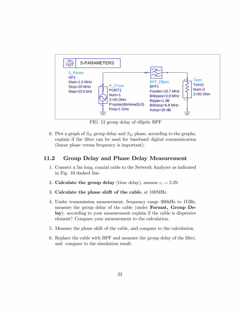
S_ParamSP1

Step=10.0 kHzStop=20 MHzStart=1.0 MHz

S-PARAMETERS

BPF_EllipticBPF1

Astop=20 dBBWstop=6.8 MHzRipple=1 dBBWpass=3.8 MHzFcenter=10.7 MHz

P_1TonePORT1

Freq=1 GHzP=polar(dbmtow(0),0)Z=50 OhmNum=1

TermTerm2

Z=50 OhmNum=2

FIG. 12 group delay of elliptic BPF

6. Plot a graph of S21 group delay and S21 phase, according to the graphs,explain if the lter can be used for baseband digital communication(linear phase versus frequency is important).

11.2 Group Delay and Phase Delay Measurement

1. Connect a 5m long, coaxial cable to the Network Analyzer as indicatedin Fig. 10 dashed line.

2. Calculate the group delay (time delay), assume r = 2:29:

3. Calculate the phase shift of the cable, at 100MHz.

4. Under transmission measurement, frequency range 300kHz to 1GHz,measure the group delay of the cable (under Format, Group De-lay). according to your measurement explain if the cable is dispersiveelement? Compare your measurement to the calculation.

5. Measure the phase shift of the cable, and compare to the calculation.

6. Replace the cable with BPF and measure the group delay of the lter,and compare to the simulation result.

22

12 Final Report

Using your data and mathematics software, or spreadsheet answer the fol-lowing Questions.

1. Attached the graphs that you save, and answer the question of the textLab.

2. Draw a graph of return loss (S11 in dB)based on measurement as afunction of frequency of the Elliptic lter. Calculate the worst SWR ofthe cable. in the passband (9.5 to 11.5 MHz).

3. Use the data of the lter to ll the following S parametrsmatrices,determine

[S] @C:F =

S11 S12S21 S22

[S] @8:5MHz =

S11 S12S21 S22

(a) If the lter is matched, reciprocal, and lossless at center frequency.

(b) If the lter is matched, reciprocal, and lossless at 8.5MHz.

23