network design for two-day e-commerce fulfillment
TRANSCRIPT

1
Network Design for Two-Day E-Commerce Fulfillment
by
Cosmo Valentino
Master of Science in Industrial Engineering, Politecnico di Milano
and
Ryan Wilson
Bachelor of Science in Business Administration, California State University of Long Beach
SUBMITTED TO THE PROGRAM IN SUPPLY CHAIN MANAGEMENT
IN PARTIAL FULFILLMENT OF THE REQUIREMENTS FOR THE DEGREE OF
MASTER OF APPLIED SCIENCE IN SUPPLY CHAIN MANAGEMENT
AT THE
MASSACHUSETTS INSTITUTE OF TECHNOLOGY
June 2021
© 2021 Cosmo Valentino and Ryan Wilson. All rights reserved.
The authors hereby grant to MIT permission to reproduce and to distribute publicly paper and electronic
copies of this capstone document in whole or in part in any medium now known or hereafter created.
Signature of Author: ____________________________________________________________________
Department of Supply Chain Management
May 14, 2021
Signature of Author: ____________________________________________________________________
Department of Supply Chain Management
May 14, 2021
Certified by: __________________________________________________________________________
Matthias Winkenbach
Director, MIT Megacity Logistics Lab
Capstone Advisor
Certified by: __________________________________________________________________________
Milena Janjevic
Research Scientist
Capstone Co-Advisor
Accepted by: _________________________________________________________________________
Prof. Yossi Sheffi
Director, Center for Transportation and Logistics
Elisha Gray II Professor of Engineering Systems
Professor, Civil and Environmental Engineering
Cosmo Valentino
Ryan Wilson

2
Network Design for Two-Day E-Commerce Fulfillment
by
Cosmo Valentino
and
Ryan Wilson
Submitted to the Program in Supply Chain Management
on May 14, 2021 in Partial Fulfillment of the
Requirements for the Degree of Master of Applied Science in Supply Chain Management
ABSTRACT
With the fast growth of e-commerce, online shoppers are becoming accustomed to free and fast delivery.
Small and medium-sized businesses are experiencing rising transportation costs as they are having to switch
from slower methods of shipping to fast delivery options (e.g., next day or two-day) to cater to customer
demand. Our sponsoring company is a 3PL providing services for these types of businesses and is currently
operating five fulfillment centers. They are looking to propose a two-day delivery service to their e-
commerce customers. To do that, the company requires an optimization model that recommends the
location and the number of fulfillment centers to activate for a given client to meet demand within a two-
day window and with a high on-time performance, while minimizing the total logistic cost. The model also
balances the tradeoff between inventory and transportation cost. In this capstone project we elaborate such
an optimization model and apply it to two customers with different shipping profiles. The results show that
the outbound transportation was identified as the most significant portion of the overall logistics spend.
This was especially true when the item being shipped was dense causing a higher rate per shipment. Inbound
and inventory cost became more significant with low-velocity items and regions with low demand. By
opening five fulfillment centers, Customer 1 would save 8.4% and by opening four fulfillment centers,
Customer 2 would save 36.1%. A 3PL can use this model to balance the inventory savings realized by a
centralized network with the transportation costs savings achieved by a decentralized configuration.
Capstone Advisor: Matthias Winkenbach
Title: Director, MIT Megacity Logistics Lab
Capstone Co-Advisor: Milena Janjevic
Title: Research Scientist

3
Acknowledgments
We would like to thank our advisors Matthias Winkenbach and Milena Janjevic for the discussions, the
insights and the guidelines we’ve received during the capstone. They both played a key role for the success
of this project.
Thanks to our sponsoring company that provided a great problem to tackle and supported us during those
months.
Cosmo
I couldn’t have accomplished this amazing achievement without my family and without all the people that
are part of my life. Special thanks my friends of NEUVASS, Gli Amici di Pippo, Non è più vacanza and to
all the friends I met at MIT and at Polimi.
To Viviana, you’re special.
Ryan
I want to thank my wife Cassie for her support and for taking care of our children while I attended class
and studied. Thank you to my two sons Johnny and Mikey who always brighten my day. Thank you to my
brother, sisters, and friends for their encouragement.

4
Contents
List of Tables .................................................................................................................................. 6
List of Figures ................................................................................................................................. 8
1. Introduction ........................................................................................................................... 10
1.1. Background ................................................................................................................... 10
1.2. Motivation ..................................................................................................................... 11
1.3. Research Problem ......................................................................................................... 12
2. Literature Review .................................................................................................................. 14
2.1. Introduction ................................................................................................................... 14
2.2. Facility Location Models .............................................................................................. 15
2.3. The Role of Inventory ................................................................................................... 16
2.3.1. Inventory Management Theory............................................................................. 17
2.3.2. Integrating Inventory Decisions in Network Design Models ............................... 19
2.4. Transportation Modes ................................................................................................... 23
2.5. Optimization of Facility Location Models .................................................................... 24
2.6. Summary ....................................................................................................................... 25
3. Methodology .......................................................................................................................... 27
3.1. Overview ....................................................................................................................... 27
3.2. Scope Definition and Data Aggregation ....................................................................... 27

5
3.3. Data Analysis and Preparation ...................................................................................... 31
3.3.1. Client Activity Data .............................................................................................. 32
3.3.2. Shipping Data of Parcel Carriers .......................................................................... 33
3.3.3. Shipping Rates of Parcel Carriers ......................................................................... 35
3.4. Optimization Model ...................................................................................................... 37
3.4.1. Overview ............................................................................................................... 37
3.4.2. Inventory Costs Modeling..................................................................................... 39
3.4.3. Mathematical Formulation .................................................................................... 45
3.4.4. Implementation ..................................................................................................... 50
4. Results & Discussion ............................................................................................................. 51
4.1. Scenario Comparison .................................................................................................... 51
4.1.1. Fizz Optimized Network ....................................................................................... 54
4.1.2. BB Optimized Network ........................................................................................ 57
4.2. Sensitivity Analysis ...................................................................................................... 63
4.2.1. Changes in Customer Demand.............................................................................. 64
4.2.2. Changes in Fulfillment Policy .............................................................................. 67
4.2.3. Changes in Inbound Transportation Costs ............................................................ 68
5. Conclusion ............................................................................................................................. 70
References ..................................................................................................................................... 72

6
List of Tables
Table 1. Number of research papers by classification dimension ................................................ 16
Table 2. Safety factor calculation for Normal Distribution .......................................................... 18
Table 3. Summary Statistics for Fizz and BB ............................................................................... 28
Table 4. Order Types for BB and Fizz .......................................................................................... 30
Table 5. Summary on data aggregation ........................................................................................ 31
Table 6. Summary of data sources ................................................................................................ 32
Table 7. Sample of the Parcel Rate Structure (Not Actual Rates) ................................................ 36
Table 8. Storage Rates by Turns (Not Actual Rates) .................................................................... 38
Table 9. Total Stock results for Fizz and BB ................................................................................ 42
Table 10. Model notation for sets and indices .............................................................................. 45
Table 11. Model notation for decision variables .......................................................................... 45
Table 12. Model notation for costs and logistics parameters........................................................ 46
Table 13. Components of the Objective Function ........................................................................ 48
Table 14. Scenario Comparison Outline ....................................................................................... 52
Table 15. Sensitivity Analysis ...................................................................................................... 64
Table 16. Sensitivity to demand volume....................................................................................... 64
Table 17. Sensitivity to demand variability .................................................................................. 66
Table 18. Sensitivity to fulfillment policy .................................................................................... 67

7
Table 19. Sensitivity to inbound transportation costs ................................................................... 69
8
List of Figures
Figure 1. Literature Review Map .................................................................................................. 14
Figure 2. Inventory Cost as a function of the Product Throughput (Shapiro, 2006) .................... 20
Figure 3. Linear Approximation for the Inventory function (Shapiro, 2006) ............................... 21
Figure 4. Square Root (Maister, 1976) ......................................................................................... 22
Figure 5. Methodology.................................................................................................................. 27
Figure 6. Weight Distribution for BB and Fizz ............................................................................ 30
Figure 7. Inventory Dynamics for BB .......................................................................................... 33
Figure 8. Historical on-time performance, Ground ...................................................................... 35
Figure 9. Methodology for Inventory Costs Calculation .............................................................. 39
Figure 10. Daily Demand - Fizz ................................................................................................... 40
Figure 11. Daily Demand Distribution - BB ................................................................................. 41
Figure 12. Inventory Costs with SRL - Fizz ................................................................................. 43
Figure 13. Inventory Costs with SRL - BB................................................................................... 44
Figure 14. Example of FTL cost structure (with maximum FTLs = 3) ........................................ 49
Figure 15. Optimized Network Configuration - Fizz.................................................................... 54
Figure 16. Scenario Cost Comparison for Fizz ............................................................................. 56
Figure 17 On-time performance Comparison for Fizz ................................................................. 57
Figure 18. Optimized Network Configuration – BB, Small Orders ............................................. 58

9
Figure 19. Optimized Network Configuration – BB, Medium Orders ......................................... 58
Figure 20. Optimized Network Configuration – BB, Large Orders ............................................. 59
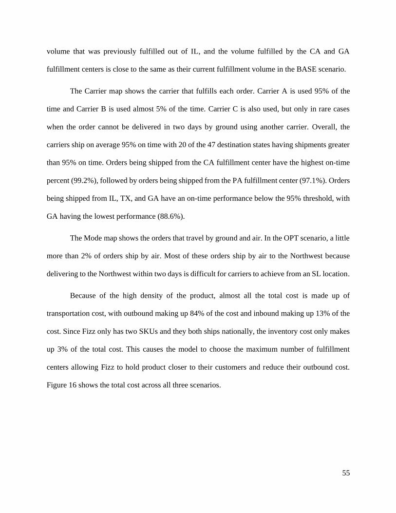
Figure 21. Scenario Cost Comparison for BB .............................................................................. 60
Figure 22. On-time performance comparison for BB ................................................................... 62
Figure 23. Inventory Function with different variability scenarios .............................................. 66

10
1. Introduction
1.1. Background
Our sponsor is a supply chain management company that provides transportation and warehousing
solutions to small and medium-sized businesses (SMBs) in the United States. For confidentiality,
we will refer to our sponsoring company as Sandoval Logistics (SL). Since SL began, their
customer base has been mainly companies that ship business to business (B2B). With the
accelerated growth of e-commerce, they would now like to further expand their customer base to
include a greater number of companies that ship business to consumer (B2C). SL’s current B2C
clients fall into two categories:
1. Direct-to-Consumer (DTC) – Product is sold on the seller’s website and is then shipped
directly to the consumer. The speed of delivery is to be determined by the consumer.
2. Seller Fulfilled Prime (SFP) – Product is sold on Amazon’s website and is then fulfilled
from SL’s fulfillment center(s). Seller is required to book shipments through Amazon’s
shipping platform to ensure compliance with delivery constraint. Seller’s products must
be delivered within 1-2 days.
SL has five fulfillment centers that are available for e-commerce fulfillment: Los Angeles, CA;
Chicago, IL; Dallas, TX; Scranton, PA; and Atlanta, GA. B2C clients ship product from their
manufacturing plant to one or more of these fulfillment centers to hold inventory. When a
consumer purchases a client’s product, the product is picked and packed as needed and then
delivered. The client chooses which third-party parcel carrier they would like to use (up to three
carriers) and the delivery mode is dictated by either the client or the consumer. The delivery mode
selection determines how a parcel order is delivered to the end customer. A parcel order can be

11
delivered using several services, including Ground 1-5 Day delivery and 2nd Day Air delivery.
Typically, the cheapest carrier will be chosen, but the on-time performance of the carrier is also
taken into consideration.
An important business capability for SL is being able to manage the network design process
on behalf of their clients. During the request for proposal (RFP) stage, SL makes the key decision
to determine the number of fulfillment centers that will be leveraged for their client’s B2C business
and which locations will be used. Currently, these decisions are taken in a manual and unstructured
way, mainly based on past experience and without the support of any analytics model.
Decisions around the facility location are extremely important both on the cost and revenue
side. 80% of the supply chain cost is determined by the location of the facilities and by the
configuration of the product flows between them (Watson et al., 2013). Companies that revise and
optimize their network can expect to see a 5 to 15% savings on their total supply chain costs
(Watson et al., 2013). On the revenue side, facility location decisions determine the delivery time
to customers and influences customer satisfaction. This relationship is particularly critical for e-
commerce businesses, where customers have high service level expectations and consider logistic
performance a key factor of the e-commerce experience (Yu et al., 2016).
1.2. Motivation
Online shoppers in the United States are becoming accustomed to free and fast delivery: 39% of
shoppers now expect companies to offer free two-day shipping for online purchases (National
Retail Federation, 2019). This trend in shipping has become known as the “Amazon Effect” and
can be attributed to the growth of Amazon Prime, a paid subscription service that offers one-to-
12
two-day free shipping to its 112 million Prime members located in the United States (CIRP, 2020).
The “Amazon Effect” has given consumers the expectation that deliveries for online purchases
should be free and quick no matter the size of the company.
SMBs have experienced rising transportation costs as they are having to switch from slower
methods of shipping to two-day shipping to cater to customer demand (Panko, 2019). Large
companies, such as Amazon and Walmart, have a national footprint of warehouses and are well
positioned to deliver to their customers in a short delivery window. The warehouse network of
SMBs can be insufficient (due to the large investment needed) and deliveries must travel longer
distances and sometimes from a single origin point to get to the homes of customers.
Fast delivery service can be a restriction that companies need to comply with (e.g. SFP), but
it can also be an internal constraint created by management in order to satisfy and attract new
customers. This service is important because not having free two-day shipping can cause shoppers
to back out of a purchase 29% of the time (National Retail Federation, 2019). For SMBs to stay
afloat in this new environment, they will need to either open new warehouse locations or partner
with third-party logistics (3PL) provider(s) to get closer to their end customer.
1.3. Research Problem
The objective of this capstone project is to formulate and solve an optimization model that allows
SL to design an optimal supply network for their e-commerce clients under a two-day delivery
window. The optimization model aims at finding the supply network configuration that minimizes
the overall network costs (inbound transportation, inventory, and outbound transportation), while
using SL’s five e-commerce fulfillment centers to satisfy all customer demand with a high level
13
of service. The model incorporates the use of third-party parcel carriers for the last mile delivery.
The rate structure for these third-party carriers is nonlinear and the deliveries can be made via
ground or air. The problem is formulated as a Mixed Integer Linear Programming (MILP) model
and solved using a numerical solver. The implementation of the model will help SL be competitive
in the bidding process for new business and it will also ensure that their e-commerce clients are in
the lowest cost solution.
The research question we answer is: What is the optimal network solution for a company
to use for delivering online orders to their customers within a two-day window while minimizing
cost and maintaining an on-time performance of at least 95%?
Our model is intended to support key decisions that SL must make when acquiring a new e-
commerce client. First, it is important to decide which fulfillment centers to use to fulfill a demand
flow coming from a specific region of the US. Moreover, SL must determine which third-party
carrier should be selected and which delivery mode (air vs. ground) should be deployed to serve
the end customers. In finding the optimal network configuration, the model considers different
types of costs: transportation cost from client manufacturing plant to SL’s fulfillment centers
(inbound), transportation cost from SL’s fulfillment centers to end customers (outbound) and
inventory holding cost at SL’s fulfillment center. Delivery speed is a very important component
of the model: the optimal network configuration must guarantee that end clients are served within
two days and with an on-time performance of at least 95%.

14
2. Literature Review
2.1. Introduction
We conduct a literature review outlined in Figure 1. The first section of our literature review
provides an overview of the key features of facility location models and the dimensions that apply
to our research. The next section analyzes the decisions that are typically taken when using facility
location models. We drill down on the decisions that are relevant to our research: inventory and
transportation modes. Even though transportation modes are different than delivery modes, the
same modeling approaches can be used to address them. The last section looks at the existing
optimization techniques used to solve our model.
Figure 1. Literature Review Map

15
2.2. Facility Location Models
Facility location models can be classified according to four key features (Melo et al., 2009):
• Number of facility layers: Determines how many nodes are visited in sequence by a product
when moving downstream to the end-customer. The number of layers usually depends on
the industry in which a company operates.
• Single vs. multiple commodities: The number of products (e.g. SKUs) included in the
model.
• Single vs. multiple periods: The planning horizon can either be a single timeframe (e.g. a
year, a quarter, a month) or a sequence of multiple time periods.
• Deterministic vs. stochastic parameters: Typical parameters that can be considered
stochastic are customer demand, lead times and transportation costs.
The study of facility location models available in literature changes dramatically according to the
four classification dimensions - see Table 1, adapted from Melo et al. (2009). The left side of the
table shows a concentration of research focused on single period and deterministic models. The
right side of the table shows that multi period stochastic models have not yet received much
attention. The research for SL is a single layer, multi commodity, single-time period, deterministic
model.

16
Table 1. Number of research papers by classification dimension
Single Period Multi Period
Layers Commodities Deterministic Stochastic Deterministic Stochastic
Single
Single 11 7 5 -
Multiple 5 - 3 -
2 Layers
Single 20 7 - 1
Multiple 12 1 5 -
≥ 3 Layers
Single 5 - 2 -
Multiple 8 4 2 -
Total 98
Not all facility location models consider the same supply chain decisions. Melo et al. (2009)
identifies six categories of decisions that are usually included in the models (in addition to the
typical location-allocation decisions). Of the six categories, the two that we use in our research are
inventory and transportation mode. Decisions on capacity, production, procurement, and routing
are not relevant to our project.
2.3. The Role of Inventory
The managing of inventory involves two key decisions that can impact the total logistics cost of a
supply chain: determining the number of stocking locations and deciding the amount of stock to
hold at each node of the network. Companies hold inventory for many reasons. When producing
or procuring goods in batches, enterprises can achieve economies of scale, and in doing so they

17
are able to hold inventory to manage the misalignment between the cyclic/intermittent nature of
procurement and the continuous flow of end-customer demand. Keeping inventory can also protect
against demand and supply fluctuations and is useful in supporting speculative purchasing
(Nahmias & Olsen, 2015).
In the next section we present an overview of inventory management theory to further
understand how inventory decisions are taken under a tactical point of view. We then introduce
three different approaches to include inventory decision in network design models.
2.3.1. Inventory Management Theory
Before we integrate inventory into our model, it is important for us to first give an overview of the
types of inventory relevant to network optimization. These types of inventory are cycle stock,
safety stock, and pipeline inventory (Nahmias & Olsen, 2015).
Cycle stock represents the average inventory level during one order cycle. If 𝑄 is the lot
size used to replenish a warehouse that serves clients at a constant rate, the average cycle stock
over one order cycle is 𝑄/2. Since all order cycles tend to be equal between themselves, the
average cycle stock level across multiple order cycles over one year is still 𝑄/2 (Nahmias & Olsen,
2015).
Safety stock is kept as protection against demand and supply uncertainty over the
replenishment lead time. In cases of absence of lead time variability, the safety stock 𝑠 can be
determined as 𝑠 = 𝑘𝜎𝐿, where 𝑘 is the safety factor and 𝜎𝐿 is the standard deviation of the demand
over the lead time. This result does not depend on the probability distribution of lead time demand
(Silver & Peterson, 1985). There are different ways of determining the safety factor and a common
18
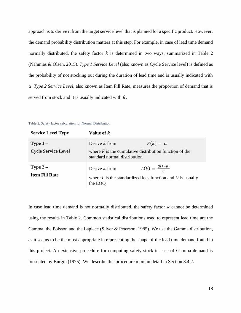
approach is to derive it from the target service level that is planned for a specific product. However,
the demand probability distribution matters at this step. For example, in case of lead time demand
normally distributed, the safety factor 𝑘 is determined in two ways, summarized in Table 2
(Nahmias & Olsen, 2015). Type 1 Service Level (also known as Cycle Service level) is defined as
the probability of not stocking out during the duration of lead time and is usually indicated with
𝛼. Type 2 Service Level, also known as Item Fill Rate, measures the proportion of demand that is
served from stock and it is usually indicated with 𝛽.
Table 2. Safety factor calculation for Normal Distribution
Service Level Type Value of 𝒌
Type 1 –
Cycle Service Level
Derive 𝑘 from 𝐹(𝑘) = 𝛼
where 𝐹 is the cumulative distribution function of the
standard normal distribution
Type 2 –
Item Fill Rate
Derive 𝑘 from 𝐿(𝑘) = 𝑄(1−𝛽)
𝜎
where 𝐿 is the standardized loss function and 𝑄 is usually
the EOQ
In case lead time demand is not normally distributed, the safety factor 𝑘 cannot be determined
using the results in Table 2. Common statistical distributions used to represent lead time are the
Gamma, the Poisson and the Laplace (Silver & Peterson, 1985). We use the Gamma distribution,
as it seems to be the most appropriate in representing the shape of the lead time demand found in
this project. An extensive procedure for computing safety stock in case of Gamma demand is
presented by Burgin (1975). We describe this procedure more in detail in Section 3.4.2.

19
Pipeline or in-transit inventory arises because moving goods from one place to another takes
time. The longer the transportation time, the higher the value of pipeline inventory. If 𝐿 is the lead
time between a supplier and a warehouse and 𝜆 is the customer demand in units per period, pipeline
inventory is 𝜆𝐿. Pipeline inventory can usually be neglected when the lead time and/or the product
value are small. In our case, replenishment lead time tends to be small and we will exclude pipeline
inventory from our analysis.
2.3.2. Integrating Inventory Decisions in Network Design Models
This section explores the available approaches for including inventory costs in network models
and identifies how they can support the resolution of the problem that SL is facing.
The main factor that pushes for the inclusion of inventory decisions in network design
problems is the risk pooling effect. When inventory is centralized (i.e. held at a central distribution
hub rather than across multiple peripheral warehouses), the risk pooling effect reduces demand
variance, resulting in lower total inventory costs (Schmitt et al., 2014). For example, if the demand
of customer 𝑖 is normally distributed with mean 𝜇𝑖 and standard deviation 𝜎𝑖, the total inventory
cost in a decentralized network with 𝑛 retailers is 𝐾 ∙ ∑ 𝜎𝑖𝑖 , where 𝐾 represents a constant number
used to consider the holding and penalty cost and the standard normal loss function. If the demand
from the 𝑛 retailers is independent (covariance equal to 0), the total inventory cost in a centralized
network is 𝐾√∑ 𝜎𝑖2
𝑖 . Under a pure inventory perspective, the centralized network is more
convenient because √∑ 𝜎𝑖2
𝑖 < ∑ 𝜎𝑖𝑖 .

20
Research that focuses on including inventory in network problems belongs to three macro-
categories: (i) models based on the inventory-throughput function (ii) models based on nonlinear
inventory costs (iii) models based on the Square Root Law. The objective of this literature review
is to select the most appropriate approach based on SL’s business and use it for the optimization
model.
The inventory-throughput function is an approach proposed by Shapiro (2006). It is built
on the idea that inventory costs for an item at a warehouse can be represented as a function of the
throughput. The main property of this function is that marginal inventory cost decreases as the
throughput increases, as shown in Figure 2.
Figure 2. Inventory Cost as a function of the Product Throughput (Shapiro, 2006)
Shapiro (2006) also suggests that the analytical function between throughput and inventory is
exponential: 𝐼 = 𝛼𝑇𝛽, where 𝐼 is the inventory level, 𝑇 the throughput and 𝛼 and 𝛽 are two
parameters that can be estimated using empirical observations. Usually, 𝛽 ranges from 0.5 and 0.8,
while 𝛼 is a positive number. The same author suggests that this empirical relationship is valid for
safety stock, cycle stock and for both combined.

21
The exponential nature of the inventory-throughput function makes it difficult to be used
for optimization, as linear models are usually easier to handle. To overcome this problem, the
original function can be broken down into multiple linear pieces that can be included in linear
optimization models with binary variables (see Figure 3).
Figure 3. Linear Approximation for the Inventory function (Shapiro, 2006)
The linear approximation also offers the opportunity to model fixed costs by using an intercept
greater than zero. The drawback of piecewise approximation is that it increases the number of
decision variables in a model. For example, the piecewise linear approximation in Figure 3 requires
three additional binary variables on top of the basic model. In a problem with 𝑥 products and 𝑛
stocking locations, the total number of incremental decision variables needed for the linear
approximation of a three-pieces function would be 3𝑥𝑛.
A second approach used to include inventory costs in optimization models is to embed the
safety stock costs directly into the objective function. However, the safety stock formulation is
based on the probability distribution function of the customer demand (see safety stock explanation
in Section 2.3.1) and forces the model to become nonlinear. An example of this approach is
proposed by Daskin et al. (2002). The authors included a nonlinear safety stock term in the cost

22
function, modeling a continuous-review (𝑄, 𝑅) policy, where 𝑄 is predetermined as the standard
EOQ and is not optimized.
The third approach is the Square Root Law. The Square Root Law claims that centralizing
inventory reduces the cycle stock because less inbound deliveries are needed and reduces the safety
stock due to the risk pooling effect on the demand (Maister, 1976). In such a context, the expected
variation is not linear but follows as a square root function. If 𝑆𝑆1 is the total safety stock required
for a product when all the stock is centralized in a single location, the total safety stock in a network
where inventory is decentralized across 𝑁 different locations is 𝑆𝑆𝑛 = 𝑆𝑆1√𝑁, as shown in Figure
4. For example, when increasing the number of locations from one to three, the expected increase
in total safety stock is a factor of √3 . The same considerations apply to cycle stock when the
reorder policy is based on the EOQ (Maister, 1976).
Figure 4. Square Root (Maister, 1976)
The Square Root Law is appropriate to use when two assumptions are met. The variance in demand
of a product is the same in every location (or varies slightly) and the demand is independent across
the locations. The model created by Croxton and Zinn (2005) in their journal article “Inventory
Considerations in Network Design” is an example of how the Square Root Law can be used to
0 1 2 3 4 5 6 7 8 9 10 11
Annual
Saf
ety S
tock
Hold
ing C
ost
N = Number of Locations Where the Product is Held
𝑆𝑆1 ∙ √𝑁
𝑆𝑆1
23
include inventory costs in network design models and we see this as being the best approach to
use in our model.
2.4. Transportation Modes
Different types of transportation modes can be selected for various reasons. The transportation
mode can be dictated by cost, the origin-destination pairing of an order, the size of an order, and
the customer service level that a company would like to target (Jayaraman, 1998). The
transportation mode can be chosen based on its environmental impact and the amount of carbon
dioxide released (Fareeduddin et al., 2015).
The transportation mode can also be selected for compliance reasons and to avoid fees.
Retailers may have guidelines published in their routing guide that call for specific shipping modes
to be used when the weight or case quantity of an order meets a certain threshold. For example,
CVS Pharmacy allows vendors to ship an order with multiple packages parcel if the case quantity
is 30 cases or less but requires vendors to ship less-than-truckload (LTL) thereafter (CVS
Pharmacy, 2020).
Eskigun et al. (2006) designed a network model around mode selection and lead time. They
found that dwell time made up a large percent of the lead time and played a role in whether an
order would be shipped by truck or rail. Even though the transportation cost to ship by rail was
less, it was better to ship by truck to minimize the lead time.
In our model, mode selection is going to be considered with the goal of maintaining an on-
time performance greater than 95% for deliveries within a two-day window. SL uses three parcel
carriers, and each carrier offers ground and air shipping options. The choice of carrier and mode
24
will depend on the origin, destination, the on-time performance for the region and the weight of
the order. Because the cost of shipping by air can range from 50-350% higher than shipping by
ground, shipments will likely only travel by air when moving cross-country since being on-time
will not be feasible through ground transportation. When shipping regionally, shipments will
always be delivered by ground if all the constraints in our model are met.
2.5. Optimization of Facility Location Models
Mathematical optimization is the most used technique to solve network design problems (Watson
et al., 2013). One class of mathematical optimization methods is linear programming (LP). A linear
program is composed by an objective function to minimize or maximize, a set of decision variables
and a series of constraints. The problem is said to be linear if the relationships between the decision
variables is linear in both the objective function and the constraints. Decision variables can either
be continuous, integer, or binary. When integer or binary variables are used, the program becomes
a MILP (Mixed-Integer Linear Program). The objective of running a MILP is to find an optimal
solution, that is, a specific set of values for the decision variables that optimize the objective
function while respecting all the constraints (Bertsimas & Tsitsiklis, 1997).
When the linearity of a model is lost, the resolution of the model is much harder and
algorithms that are specifically designed for nonlinear optimization must be implemented instead.
For example, Lagrangean relaxation and Lagrangean decomposition methods have found a wide
application in solving supply chain optimization problems (You & Grossmann, 2008).
25
In the case of our project, we decide to keep the model linear and to solve the design problem
using a Mixed Integer Linear formulation. SL will need to run our model frequently with solution
time, usability, and scalability being key factors for a successful implementation of this approach.
2.6. Summary
SL should turn to network design when acquiring new e-commerce clients. In our research we use
a facility location model that consists of a single layer, multi commodity, single period, and
deterministic dimensions as it most closely resembles the business of SL’s clientele. Our research
includes three modeling elements that are usually neglected in the context of supply chain network
design: inclusion of inventory costs, selection of delivery mode and carrier, compliance with a
target of on-time performance on the carrier deliveries.
Relationships involving inventory are difficult to include in optimization models and are
often overlooked (Shapiro, 2006), mainly because of their nonlinear nature. However, ignoring
inventory costs in network design models is commonly recognized as a limitation and is one of the
“worst features” of network optimization problems (Croxton & Zinn, 2005). Three approaches are
available in the literature to overcome this limitation: (i) models based on the inventory-
throughput function (ii) models based on nonlinear inventory costs (iii) models based on the
Square Root Law.
The Square Root Law is the most promising approach to solve the problem of SL.
Compared to the linear approximation of inventory costs, this method does not require an empirical
estimation of the inventory-throughput function. Clients rarely share historical inventory snapshots
during the proposal process, and it is not possible to estimate the function without this information.
26
Moreover, the Square Root Law method is easier to implement compared to using nonlinear
inventory costs in the objective function. This approach makes the problem nonlinear and requires
specific techniques and algorithms that are slower, less stable, and less “commercially pervasive”
than the ones used to solve linear problems.
Historically, the choice of delivery modes (air vs. ground) has not received much attention
(Melo et al., 2009). We include this element in the optimization model and evaluate its impact on
the overall network cost function.
Moreover, the compliance with a target on-time performance of the carrier deliveries is
generally absent from the literature and only service level in relationship to the inventory is present.
We incorporate this constraint in the model to make sure that delivery windows are respected for
the end customer.

27
3. Methodology
3.1. Overview
To find the optimal network solution for a company to use for delivering online orders to their
customers within a two-day window with a high level of service, we build a MILP using data
provided by SL as inputs. First, we familiarize ourselves with the client data and we create a list
of potential clients to focus our research on. We then collect additional data that we clean,
transform, and aggregate. Next, we build and run the model and analyze the results. Figure 5
summarizes the steps in our methodology.
Figure 5. Methodology
3.2. Scope Definition and Data Aggregation
We choose to focus our analysis on two specific clients, and for confidentiality reasons, we assign
them fictitious names here. The first is a beverage company that we refer to as Fizz; the second is
a bakery goods company that we refer to as Bread Box (BB). There are three reasons why we
choose these two companies. First, Fizz and BB are the largest B2C clients for SL and they have
the most activity available to analyze. Second, SL targets e-commerce clients that ship a minimum

28
of 600 orders per month and both companies meet this criterion. Third, both companies have a
different shipping profile, allowing us to create a diverse model (See Table 3).
Table 3. Summary Statistics for Fizz and BB
FIZZ BREAD BOX (BB)
Commodity Beverages Bakery Goods
Number of SKUs 2 36
Average Order Weight (Lbs) 31 6
Number of SKUs Per Master Carton 1 Multiple
Average Orders Per Month 3,014 2,058
Manufacturing Location (State) CA NJ
Current Fulfillment Solution 3 Fulfillment Centers:
CA, IL, GA
1 Fulfillment Center:
PA
Each Fizz stock-keeping unit (SKU) contains 12-24 bottles per case and ships individually at the
case level. These cases weigh 31 pounds and are currently fulfilled from three locations. Each
SKU for BB is sold at the unit level (e.g. one box of croissants) and can ship together with other
BB items. For example, if an order is placed for five different types of bakery goods, all five items
will be placed inside a single master carton and shipped to the customer. These packages are lighter
than Fizz packages and have a higher weight per cubic foot. They are currently being fulfilled from
a single location in the Northeast.
Now that we have selected the target companies, we shift our focus to data aggregation.
Data aggregation can be defined as putting “data into logical groups for the purpose of modeling”
(Watson et al., 2013) and is a fundamental step when designing an optimization model for two
reasons. The first reason is technical: models with aggregated data (e.g. a family of products
29
instead of a single product) are usually smaller and take less time to solve. Moreover, when a
model uses future forecasts as input data, the aggregated versions tend to be more accurate because
grouped forecasts are usually more reliable than line-level forecasts. The second reason is
practical: models that include too much detail make it difficult to understand the big picture and
getting data at a detailed level can be time consuming or even impossible. For our model, we
aggregate the data for three different dimensions: products, customers, and time.
Product aggregation. We build a model based on customer orders and not on the number of
units being shipped. The reasons are the following:
• Orders mimic customer demand very closely. Although customers order at the item level,
e-commerce sellers typically consolidate the units of an order into a single master carton
when possible at the time of shipping.
• Each master carton is associated with one parcel order. B2C orders containing more than
one master carton are infrequent for SL.
• Parcel carriers bill based on the weight of the master carton and not on each of the
individual items contained inside.
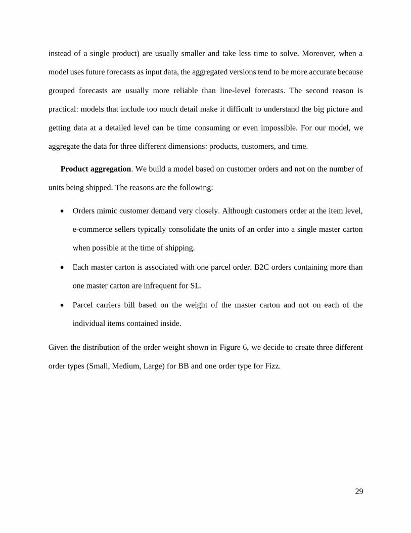
Given the distribution of the order weight shown in Figure 6, we decide to create three different
order types (Small, Medium, Large) for BB and one order type for Fizz.

30
Figure 6. Weight Distribution for BB and Fizz
The thresholds for the BB order types are included in Table 4. We are able to use a constant weight
of 31 pounds for Fizz since they only ship two SKUs (one unit per master carton) and each SKU
weighs 31 pounds.
Table 4. Order Types for BB and Fizz
Company Order
Type
Weight Range
(lbs) %
Avg. Weight
(lbs)
Number of SKUs
per order
BB Small 0 to 5 incl. 37% 2.5 avg: 4.6 - std: 2.8
BB Medium 5 to 10 incl. 58% 7.5 avg: 10.9 - std: 2.6
BB Large 10 to 15 incl. 5% 12.5 avg: 16.1 - std: 3.8
Fizz - - 100% 31 1
Customer aggregation. We use the first three digits of the destination zip code as a
customer dimension. This aggregation has no effect on accuracy of cost and it is in line with how
parcel carriers bill. It also reduces the number of decision variables and it allows our model to have
a more consistent and reliable estimate of the demand compared to using all five digits of the zip
code.

31
Time period aggregation. The time buckets that are usually used for network design are
yearly, monthly or weekly. We use one single time period with annualized variables. The main
reason behind this decision is that customer demand does not show a strong seasonal effect for the
two target companies selected. Moreover, SL rarely receives enough data to estimate seasonal
patterns when bidding new clients. In such a context, a single period model is more appropriate.
The modeling decisions made with respect to each dimension are summarized in Table 5.
Table 5. Summary on data aggregation
Dimension Aggregation
Products
BB: Three different order types: Small, Medium, and Large. Each order type
has a different weight.
Fizz: One order type with an average weight of 31 pounds.
Customers End customer demand is grouped using the first three digits of the destination
zip code. The same approach is used for both BB and Fizz.
Time
Periods Single period model (one year).
In the next sections we summarize the data through collection, analysis, and transformation for the
clients in scope.
3.3. Data Analysis and Preparation
The data provided by SL consists of three different types of datasets: client activity, delivery
performance of parcel carriers, and shipping rates of parcel carriers. The content of each source is
summarized in Table 6.

32
Table 6. Summary of data sources
Data Source Content
Client Activity
Line-level shipments including order number, item number, date shipped,
origin zip code, destination zip code, units shipped, unit weight, and unit
cube.
Shipping Data
of Parcel
Carriers
Historical delivery records at order level with both requested and actual
delivery date.
Shipping Rates
of Parcel
Carriers
Transportation rates by weight and by delivery zone.
The following sections present an overview of the three datasets that we use and explain how we
analyze, clean, and group the data for modeling purposes.
3.3.1. Client Activity Data
The client activity is at the line-level for each order shipped and contains the order number, item
number, date shipped, origin zip code, destination zip code, units shipped, unit weight, and unit
cube. The activity data helps us build out the inventory, the inbound (manufacturer to SL’s
fulfillment center), and the outbound (SL’s fulfillment center to end customer) portions of our
model.
For inventory, we use the activity to get an understanding of the daily number of cases held
by each client by warehouse location. This is done by taking the difference between the number
of cases coming in and the number of cases going out each day. To get a more accurate
approximation of the customer demand, we do not use the entire horizon in computing the total

33
yearly demand. Instead, we select a time horizon where inventory dynamics is more stable. This
condition is more representative of the current business for Fizz and BB. For example, looking at
Figure 7, we use six months of data starting May 2020 for BB. Same considerations have been
made for Fizz.
Figure 7. Inventory Dynamics for BB
We use outbound activity to determine the demand by destination zip code. We then
transform the line-level data into order-level data and aggregate the data by the first three digits of
the destination zip code. As an example, zip codes 90815 and 90803 are grouped together since
their first three digits are the same.
Because the time frame that we use is less than a year for both clients, we annualize the
number of orders being shipped in the data before inserting them into our model.
3.3.2. Shipping Data of Parcel Carriers
SL uses three third-party carriers for all parcel shipments: Carrier A, Carrier B, and Carrier C. The
data consists of both B2B and B2C orders with most of the orders being shipped B2B.

34
Unfortunately, the data includes shipments only for Carrier A and Carrier B; data does not
currently exist for the shipments of Carrier C. Using this data, we are able to calculate with
precision the on-time performance by carrier from each fulfillment center to each destination
region of the United States only for Carrier A and Carrier B. To estimate the on-time performance
for Carrier C, we take the on-time performance calculations for Carrier A and Carrier B and take
the lower of the two. This approach was recommended to us by SL based on their experience using
Carrier C for shipping.
When the Covid-19 pandemic began, parcel carriers were flooded with orders and their on-
time performance dropped, causing them to issue statements regarding delays in shipments
(FedEx, 2020). To get a sense of the on-time performance of parcel carriers by mode under normal
shipping conditions, SL provided two years of parcel carrier shipping data ending February 2020.
It should be noted though that 100% of late deliveries may not necessarily be the fault of the carrier.
Some of these late deliveries could be due to warehouse operations or a client not having product
in stock. The data does not specify who is at fault; however, the assumption we use is that the
third-party carriers make up all the late deliveries. The on-time performance of Ground deliveries
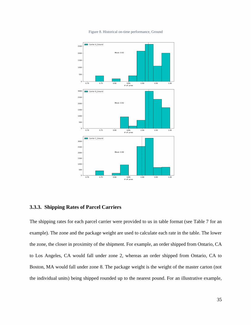
for the three carrier is shown in Figure 8. The on-time performance for Air delivery is 100% for
all the carriers.
35
Figure 8. Historical on-time performance, Ground
3.3.3. Shipping Rates of Parcel Carriers
The shipping rates for each parcel carrier were provided to us in table format (see Table 7 for an
example). The zone and the package weight are used to calculate each rate in the table. The lower
the zone, the closer in proximity of the shipment. For example, an order shipped from Ontario, CA
to Los Angeles, CA would fall under zone 2, whereas an order shipped from Ontario, CA to
Boston, MA would fall under zone 8. The package weight is the weight of the master carton (not
the individual units) being shipped rounded up to the nearest pound. For an illustrative example,

36
if an order is going to zone 5 and the weight of the master carton is 1.25 pounds (rounded up to 2
pounds), the rate that will be used in Table 7 is Rate 11.
Table 7. Sample of the Parcel Rate Structure (Not Actual Rates)
Zone
Package Weight (lbs) 2 3 4 5 6 7 8
1 Rate 1 Rate 2 Rate 3 Rate 4 Rate 5 Rate 6 Rate 7
2 Rate 8 Rate 9 Rate 10 Rate 11 Rate 12 Rate 13 Rate 14
SL provided us with their contract agreements with their parcel carriers. We find that the rates
provided for Carrier 3 are inclusive of fuel and additional surcharges; however, the rates provided
for Carrier 1 and Carrier 2 are not. There are also additional discounts in the Carrier 1 and Carrier
2 contracts that have not yet been applied to the rates. We apply these adjustments to the rates for
Carrier 1 and Carrier 2 to ensure that a fair comparison can be made with the Carrier 3 rates.
While developing the rates for our model, we also consider dimensional weight, which can
be defined as the amount of space a package uses relative to the actual weight of the package (UPS,
2020). Dimensional weight is calculated by multiplying the length, width, and height of the
package and then dividing by a dimensional divisor that is unique to the carrier being used. The
carrier then compares the dimensional weight and the actual weight of the package and uses the
greater of the two for billing. Since dimensional pricing does not apply to high density product,
dimensional pricing is not applied to the rates for Fizz and is only factored into the rates for BB.
37
3.4. Optimization Model
3.4.1. Overview
A MILP model is constructed to find the optimal network configuration. The objective function,
to be minimized, is the sum of three cost components: inbound transportation, outbound
transportation, and inventory.
Inbound Transportation Cost: The client ships goods from its manufacturer to the
fulfillment center operated by SL. This transportation flow is typically done using FTL (Full-
Truckload) road freight services. FTL rates for a specific lane are estimated by using spot rates
available on public load boards.
Outbound Transportation Cost: The products that are stocked at SL’s fulfillment centers
are shipped to the end customers as parcel deliveries using third party carriers. Each carrier charges
a specific delivery rate that varies by weight and distance as explained in the “Shipping Rates of
Parcel Carriers” section.
Inventory Cost: The inclusion of inventory costs will ensure balancing the trade-off
between savings from centralization and extra costs generated by using fastest delivery modes. As
explained in the beginning of Section 2.3.2, centralizing inventory reduces the total stock due to
the risk pooling effect and the reduction follows the nonlinear Square Root Law. However,
centralizing stock usually means being farther from clients and achieving high level of service in
such a context can be more expensive and might require the use of expresses delivery modes. Our
model analyzes this trade-off to find the optimal solution.
In our case, inventory costs are incurred when products are stored in SL’s fulfillment
centers. When this happens, the client is billed a set of storage rates by SL. The storage rates are
38
billed at the pallet level and are uniform across all fulfillment centers. Initial storage is billed when
a pallet arrives at the fulfillment center and recurring storage is billed on the first day of the month
for each pallet that is held in the fulfillment center. The rate that is billed for initial and recurring
storage depends on how fast inventory turns over. Slow moving inventory is billed at a higher rate.
Inbound handling is billed similarly to initial storage as it is billed when a pallet arrives at the
fulfillment center; however, the inbound handling rate is fixed and is not affected by the turn rate
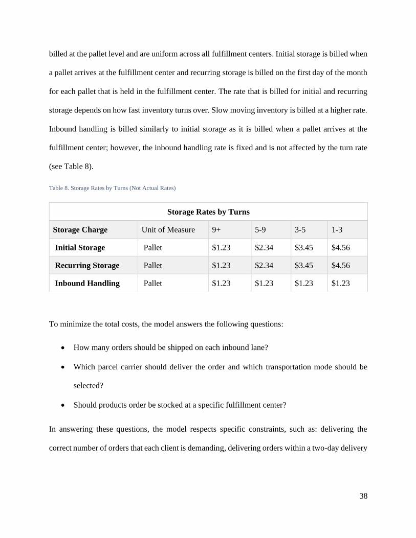
(see Table 8).
Table 8. Storage Rates by Turns (Not Actual Rates)
Storage Rates by Turns
Storage Charge Unit of Measure 9+ 5-9 3-5 1-3
Initial Storage Pallet $1.23 $2.34 $3.45 $4.56
Recurring Storage Pallet $1.23 $2.34 $3.45 $4.56
Inbound Handling Pallet $1.23 $1.23 $1.23 $1.23
To minimize the total costs, the model answers the following questions:
• How many orders should be shipped on each inbound lane?
• Which parcel carrier should deliver the order and which transportation mode should be
selected?
• Should products order be stocked at a specific fulfillment center?
In answering these questions, the model respects specific constraints, such as: delivering the
correct number of orders that each client is demanding, delivering orders within a two-day delivery
39
window, using carriers that have an acceptable on-time performance and ensuring the flow balance
at each fulfillment center.
In the next sections we present first the inventory cost modeling and then mathematical
formulation of the optimization model.
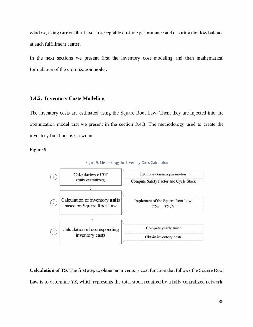
3.4.2. Inventory Costs Modeling
The inventory costs are estimated using the Square Root Law. Then, they are injected into the
optimization model that we present in the section 3.4.3. The methodology used to create the
inventory functions is shown in
Figure 9.
Figure 9. Methodology for Inventory Costs Calculation
Calculation of TS: The first step to obtain an inventory cost function that follows the Square Root
Law is to determine 𝑇𝑆, which represents the total stock required by a fully centralized network,

40
where all the stock is concentrated in a single warehouse and all demand is fulfilled from there.
Following the inventory management principles presented in the safety stock explanation of
Section 2.3.1, 𝑇𝑆 can be computed as 𝑇𝑆 = 𝑘𝜎𝐿 + 𝑄/2, where 𝑘 is the safety factor, 𝜎𝐿 is the
standard deviation of the demand over the lead time and 𝑄 is the lot size used by the client. Even
though this equation remains valid with any probability distribution of lead time demand (Silver
& Peterson, 1985), the calculation of 𝑘 depends on the specific distribution used.
The distribution of the daily demand is asymmetrical and skewed to the left for both Fizz
and BB. This is a common behavior when a stochastic variable represents a product demand. One
way of approaching this scenario is to model the empirical data using the Gamma distribution
instead of the normal distribution. The Gamma distribution takes two parameters as input, scale
𝜃 and shape 𝑘, and its probability distribution function is the following:
𝑓(𝑥) = 1
𝜑(𝑘)𝜃𝑘𝑥𝑘−1𝑒−
𝑥𝜃
We use the method of moments to fit the two parameters of the Gamma distribution that
best describe our data. The results are shown in Figure 10 for Fizz and in Figure 11 for BB.
Figure 10. Daily Demand - Fizz

41
Figure 11. Daily Demand Distribution - BB
Once the daily distribution is defined, the next step before calculating the safety factor is to
determine the lead time distribution. Burgin (1975) shows that if the daily demand follows a
Gamma function, then the lead time demand still follows a Gamma function, with the same scale
= 𝜃 but with shape = 𝑘𝐿, where 𝐿 is the lead time in days. We assume a lead time of 15 days for
both companies, as it best represents the real business scenario.
Using the lead time demand distribution, we compute the safety factor using the Gamma
cumulative distribution. Then we calculate the value of 𝑇𝑆 accordingly, summing the cycle stock
as well. Results are shown in Table 9.

42
Table 9. Total Stock results for Fizz and BB
Fizz
𝜶 (Cycle Service Level) 98.5 %
k 2.49
TS [# units] 1598.73
BB
Small Medium Large
𝜶 (Cycle Service Level) 98.5 % 98.5 % 98.5 %
k 2.43 2.40 2.42
TS [# orders] 2517.82 1395.42 505.81
Calculation of inventory units based on Square Root Law: Once 𝑇𝑆 is known, it is possible to
apply the Square Root Law to obtain the inventory requirements as a function of the number of
fulfillment centers used.
Calculation of corresponding inventory costs: The costs associated with the inventory
requirements in Table 9 must be determined keeping into consideration the non-linear structure of
the inventory costs as described in Section 3.4.1. This cost structure is based on the annual turns
and modifies the shape of the “pure” Square Root Law, as shown in Figure 12 for Fizz and in
Figure 13 for BB. This interesting behavior is particularly evident for BB, where inventory costs
nearly double when moving from one warehouse to two for Medium sized orders. In this case the

43
warehouse rate goes up +31% due to the reduction of yearly turns (see Table 8), generating a step
change in the inventory function (see Figure 13).
Figure 12. Inventory Costs with SRL - Fizz

44
Figure 13. Inventory Costs with SRL - BB
The costs included in these graphs will be plugged in the objective function of the optimization
model described in the next Section 3.4.4.

45
3.4.3. Mathematical Formulation
The mathematical notation used in the optimization model is introduced in this section. Next, the
Mixed-Integer Linear Program is presented and described in detail in all its components: objective
function, decision variables and constraints.
Notation for Sets and Indices
Table 10. Model notation for sets and indices
ELEMENT SET
Fulfillment Centers 𝐼 = { 𝑖}
Client Origins 𝑂 = {𝑜}
Order Types 𝐾 = {𝑘}
End Customers 𝐽 = {𝑗}
Modes 𝐺 = {𝐺}
Carriers 𝐻 = {ℎ}
Segments of The FTL Cost Function 𝑃 = {𝑝}
Segment of The Inventory Cost Function (Square Root Law) 𝐴 = {𝑎}
Notation for Decision Variables
Table 11. Model notation for decision variables
VARIABLE MEANING
𝒙𝒐𝒊𝒌 Flow on arcs from client origins o to fulfillment center i for order size type k
𝒚𝒊𝒋𝒌𝒈𝒉 Flow on arcs from fulfillment center i to customers j for order type k and
delivery mode g and carrier h

46
𝒔𝒊𝒌 Binary variable equal to 1 if stock of order type k is kept at the fulfillment
center i
𝒘𝒂𝒌 Binary variable equal to 1 when 𝑎 fulfillment centers are selected for the
order type k
𝒗𝒐𝒊𝒌𝒑 Binary variable used for the activation of the segment p of the FTL cost
function
𝒍𝒐𝒊𝒌𝒑 Equal to 𝑥𝑜𝑖𝑘 when it falls on the segment p of the FTL cost function
Notation for Costs and Logistics Parameters
Table 12. Model notation for costs and logistics parameters
PARAMETER MEANING
𝒄𝒊𝒋𝒌𝒈𝒉 Transportation cost to serve order k to customer j from fulfillment center i
with delivery mode g and carrier h
𝒇𝒐𝒊 FTL transportation cost from origin o to fulfillment center i
𝑫𝒋𝒌 Demand of orders k from customer j
𝒓𝒊𝒋𝒈𝒉 Historical on-time performance for the mode g and carrier h on the delivery
lane i-j. It is a number between 0 and 1
𝒉𝒊𝒋𝒈𝒉 Equal to 1 if the mode g and carrier h ensure delivery within two-days on the
outbound lane i-j
𝑵𝒌 Maximum number of FTLs needed for the order k
𝑳𝒌 Maximum number of order k that can be shipped on one FTL
𝒒𝒂𝒌 Total inventory cost across the entire network for the order type k when a
fulfillment centers are used. Follows the Square Root Law and the warehouse
rate structure
𝜹 Target on-time performance (global)
47
𝑴 Big number used for the linking constraints. 𝑀 = ∑ ∑ 𝐷𝑗𝑘𝑘𝑗
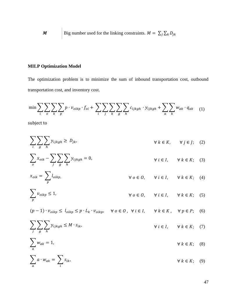
MILP Optimization Model
The optimization problem is to minimize the sum of inbound transportation cost, outbound
transportation cost, and inventory cost.
min ∑ ∑ ∑ ∑ 𝑝 ∙ 𝑣𝑜𝑖𝑘𝑝 ∙ 𝑓𝑜𝑖 +
𝑝𝑘𝑜𝑖
∑ ∑ ∑ ∑ ∑ 𝑐𝑖𝑗𝑘𝑔ℎ ∙ 𝑦𝑖𝑗𝑘𝑔ℎ
ℎ
+ ∑ ∑ 𝑤𝑎𝑘 ∙ 𝑞𝑎𝑘
𝑘𝑎
𝑔𝑘𝑗𝑖
(1)
subject to
∑ ∑ ∑ 𝑦𝑖𝑗𝑘𝑔ℎ
ℎ𝑔𝑖
≥ 𝐷𝑗𝑘 , ∀ 𝑘 ∈ 𝐾, ∀ 𝑗 ∈ 𝐽; (2)
∑ 𝑥𝑜𝑖𝑘
𝑜
− ∑ ∑ ∑ 𝑦𝑖𝑗𝑘𝑔ℎ
ℎ
= 0,
𝑔𝑗
∀ 𝑖 ∈ 𝐼, ∀ 𝑘 ∈ 𝐾; (3)
𝑥𝑜𝑖𝑘 = ∑ 𝑙𝑜𝑖𝑘𝑝,
𝑝
∀ 𝑜 ∈ 𝑂, ∀ 𝑖 ∈ 𝐼, ∀ 𝑘 ∈ 𝐾; (4)
∑ 𝑣𝑜𝑖𝑘𝑝 ≤ 1,
𝑝
∀ 𝑜 ∈ 𝑂, ∀ 𝑖 ∈ 𝐼, ∀ 𝑘 ∈ 𝐾; (5)
(𝑝 − 1) ∙ 𝑣𝑜𝑖𝑘𝑝 ≤ 𝑙𝑜𝑖𝑘𝑝 ≤ 𝑝 ∙ 𝐿𝑘 ∙ 𝑣𝑜𝑖𝑘𝑝, ∀ 𝑜 ∈ 𝑂 , ∀ 𝑖 ∈ 𝐼, ∀ 𝑘 ∈ 𝐾 , ∀ 𝑝 ∈ 𝑃; (6)
∑ ∑ ∑ 𝑦𝑖𝑗𝑘𝑔ℎ
ℎ
≤ 𝑀 ∙ 𝑠𝑖𝑘
𝑔𝑗
, ∀ 𝑖 ∈ 𝐼, ∀ 𝑘 ∈ 𝐾; (7)
∑ 𝑤𝑎𝑘 = 1
𝑎
, ∀ 𝑘 ∈ 𝐾; (8)
∑ 𝑎 ∙ 𝑤𝑎𝑘
𝑎
= ∑ 𝑠𝑖𝑘
𝑖
, ∀ 𝑘 ∈ 𝐾; (9)

48
𝑦𝑖𝑗𝑘𝑔ℎ ≤ 𝑀 ∙ ℎ𝑖𝑗𝑔ℎ, ∀ 𝑖 ∈ 𝐼 , ∀ 𝑗 ∈ 𝐽, ∀ 𝑘 ∈ 𝐾,
∀ ℎ ∈ 𝐻, ∀ 𝑔 ∈ 𝐺; (10)
∑ ∑ ∑ ∑ 𝑦𝑖𝑗𝑘𝑔ℎ ∙ 𝑟𝑖𝑗𝑔ℎℎ𝑔𝑗𝑖
∑ 𝐷𝑗𝑘𝑗≥ 𝛿, ∀ 𝑘 ∈ 𝐾; (11)
𝑣𝑜𝑖𝑘𝑝 , 𝑤𝑎𝑘 , 𝑠𝑖𝑘 ∈ {0,1}, (12)
𝑦𝑖𝑗𝑔ℎ𝑘 ≥ 0 and 𝐼𝑛𝑡, 𝑥𝑜𝑖𝑘 ≥ 0 and 𝐼𝑛𝑡, 𝑙𝑜𝑖𝑘𝑝 ≥ 0 and 𝐼𝑛𝑡. (13)
The objective function (1) minimizes the sum of the three cost components summarized in Table
13.
Table 13. Components of the Objective Function
OBJECTIVE FUNCTION COMPONENT MEANING
∑ ∑ ∑ ∑ 𝒑 ∙ 𝒗𝒐𝒊𝒌𝒑 ∙ 𝒇𝒐𝒊
𝒑𝒌𝒐𝒊
Inbound Transportation Cost
∑ ∑ ∑ ∑ 𝒄𝒊𝒋𝒎𝒌 ∙ 𝒚𝒊𝒋𝒎𝒌
𝒌𝒎𝒋𝒊
Outbound Transportation Cost
∑ ∑ 𝒘𝒂𝒌 ∙ 𝒒𝒂𝒌
𝒌𝒂
Inventory Cost
The inventory costs 𝑞𝑎𝑘 follow the law suggested by Croxton and Zinn (2005) and are pre-
computed before running the optimization model. More details on this pre-process can be found
in section 3.4.2.
49
Constraints (2) ensure the end customer demand is served, while Constraints (3) guarantee
the flow balance between inbound and outbound flows for all order types – warehouse
combinations.
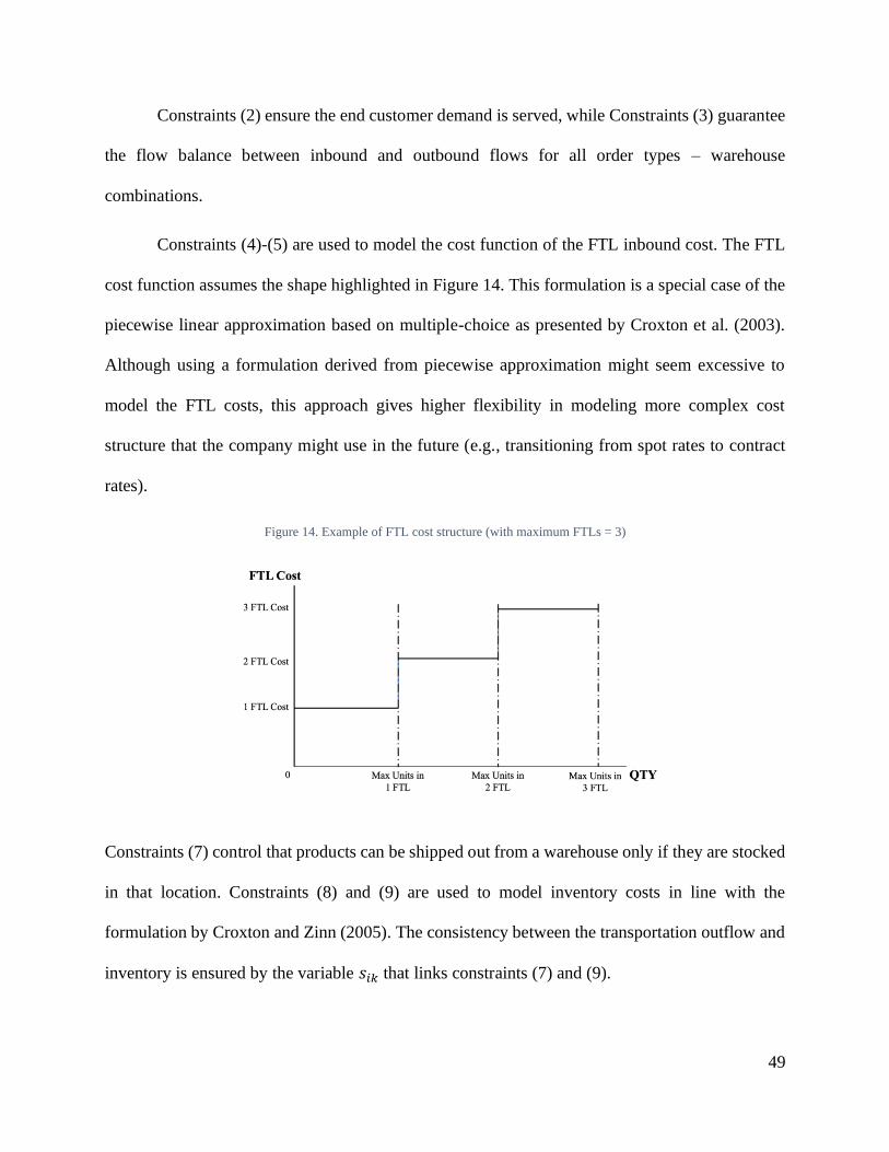
Constraints (4)-(5) are used to model the cost function of the FTL inbound cost. The FTL
cost function assumes the shape highlighted in Figure 14. This formulation is a special case of the
piecewise linear approximation based on multiple-choice as presented by Croxton et al. (2003).
Although using a formulation derived from piecewise approximation might seem excessive to
model the FTL costs, this approach gives higher flexibility in modeling more complex cost
structure that the company might use in the future (e.g., transitioning from spot rates to contract
rates).
Figure 14. Example of FTL cost structure (with maximum FTLs = 3)
Constraints (7) control that products can be shipped out from a warehouse only if they are stocked
in that location. Constraints (8) and (9) are used to model inventory costs in line with the
formulation by Croxton and Zinn (2005). The consistency between the transportation outflow and
inventory is ensured by the variable 𝑠𝑖𝑘 that links constraints (7) and (9).

50
Constraints (10) force the model to select the only the modes that guarantee delivery within
two-days, while (11) make sure that the modes are selected to achieve a global on time
performance above our target threshold.
Constraints (12) and (13) ensure that decision variables are assigned to the correct type. Since
order quantities tend to be small and no performance issues are experienced, all numeric variables
are kept as integers.
3.4.4. Implementation
The optimization model is built in Python 3.8 and is solved using Gurobi 9.1, a mathematical
solver that implements MILP optimization algorithms such as brand and bound, cutting planes,
solution improvements and others.
51
4. Results & Discussion
This capstone project builds an optimization model that SL can use when bidding on logistic
services for new clients. To evaluate the quality of the proposed model, we run three scenarios
each for Fizz and BB and compare the results. The three scenarios are the Baseline Scenario, the
Baseline with Two-Day Constraint Scenario, and the Optimized Scenario.
After comparing scenarios, we analyze how the optimal solution proposed by our model
reacts when input data such as demand, lead time, and transportations modes are changed (Section
4.2). This sensitivity analysis is critical because the data and information gathered during the
bidding process is not always reliable. Understanding how the network shifts when inputs are
modified is an important step to finalizing our model.
4.1. Scenario Comparison
We build three scenarios to understand the performance of the model for both Fizz and BB. Each
scenario is defined by four dimensions: fulfillment centers activated, carriers chosen, constraint on
the percentage of orders shipped using Two-Day service and on-time performance achieved. Table
14 outlines the scenarios along with our assumptions.

52
Table 14. Scenario Comparison Outline
Code Name Fulfillment
Centers
Number of
Carriers
% Orders
Shipped Using
Two-Day Service
On-Time
Performance
BASE Baseline Currently used
by client
Currently
used by client Not enforced Not enforced
BASE2D Baseline with
two-day service
Currently used
by client
Optimized
through
model
Enforced Enforced
OPT Optimized Optimized
through model
Optimized
through
model
Enforced Enforced
Scenario 1: Baseline Scenario (BASE2D): Four adjustments are made to mimic the
current operations for Fizz and BB. First, we enforce the SL fulfillment centers that are currently
being used (three for Fizz and one for BB) to stay open and the unused fulfillment centers to remain
closed. Next, we remove the two-day delivery service constraint and the on-time % constraint
since these are not currently hard constraints for either Fizz or BB. Finally, we add a carrier
constraint to only use the carriers that Fizz and BB currently ship with.
Scenario 2: Baseline with Two-Day Service (BASE2D): Like Scenario 1, but with a few
exceptions. All orders must ship using a two-day delivery service, all orders must be on time 95%
of the time, and the cheapest carrier is selected.
Scenario 3: Optimized Scenario (OPT): Follows all constraints laid out in the
Methodology chapter and allows the model to choose the optimal number of fulfillment centers to
be used.

53
As we compare the scenarios, SL suggests that we look at the following KPIs to see the
effectiveness of our model:
• Total annual logistic costs - (TLC). The sum of inbound transportation cost, outbound
transportation cost and inventory cost in USD. This is computed using the objective
function of the MILP model in equation (1) in Section 3.4.3.
• On-Time performance - (OTP). The global on-time performance provided by the parcel
carriers selected. As an example, if an order is expected to be delivered within five days,
the order is considered on-time if it is delivered to the customer anytime within the five-
day window. This is computed as the weighted average of the OTP on each lane used in
the network. The weights are represented by the demand:
𝑂𝑇𝑃 = ∑ ∑ ∑ ∑ ∑ 𝑦𝑖𝑗𝑘𝑔ℎℎ ∙ 𝑟𝑖𝑗𝑔ℎ𝑔𝑘𝑗𝑖
∑ 𝑦𝑖𝑗𝑘𝑔ℎ𝑖𝑗𝑘𝑔ℎ
• % Orders Shipped Using Two-Day Service - (2DS). Computed as the number of orders
shipped using a two-day delivery service divided by the total number of orders shipped:
2𝐷𝑆 = ∑ ∑ ∑ ∑ ∑ 𝑦𝑖𝑗𝑘𝑔ℎℎ ∙ ℎ𝑖𝑗𝑔ℎ𝑔𝑘𝑗𝑖
∑ 𝑦𝑖𝑗𝑘𝑔ℎ𝑖𝑗𝑘𝑔ℎ
Both OTP and 2DS follow the mathematical notation presented in 3.4.3:
• 𝑦𝑖𝑗𝑘𝑔ℎ : Flow on arcs from fulfillment center i to customers j for order type k and delivery
mode g and carrier h.
• 𝑟𝑖𝑗𝑔ℎ : Historical on-time performance for the mode g and carrier h on the delivery lane i-
j. It is a number between 0 and 1.

54
• ℎ𝑖𝑗𝑔ℎ : Equal to 1 if the mode g and carrier h ensure delivery within two-days on the
outbound lane i-j.
4.1.1. Fizz Optimized Network
The OPT network that is chosen for Fizz is a five-fulfillment center network and is summarized
in Figure 15 using three maps: Fulfillment Center, Customer Assignment, Carrier and Mode.
Figure 15. Optimized Network Configuration - Fizz
The Customer Assignment map shows where each customer order is fulfilled from. Even though
the product originates out of Southern California and one-third of the product ends up being
delivered to consumers on the West Coast, it still makes sense for product to be held in all five
fulfillment centers. The newly opened fulfillment centers in PA and TX take more than half of the
55
volume that was previously fulfilled out of IL, and the volume fulfilled by the CA and GA
fulfillment centers is close to the same as their current fulfillment volume in the BASE scenario.
The Carrier map shows the carrier that fulfills each order. Carrier A is used 95% of the
time and Carrier B is used almost 5% of the time. Carrier C is also used, but only in rare cases
when the order cannot be delivered in two days by ground using another carrier. Overall, the
carriers ship on average 95% on time with 20 of the 47 destination states having shipments greater
than 95% on time. Orders being shipped from the CA fulfillment center have the highest on-time
percent (99.2%), followed by orders being shipped from the PA fulfillment center (97.1%). Orders
being shipped from IL, TX, and GA have an on-time performance below the 95% threshold, with
GA having the lowest performance (88.6%).
The Mode map shows the orders that travel by ground and air. In the OPT scenario, a little
more than 2% of orders ship by air. Most of these orders ship by air to the Northwest because
delivering to the Northwest within two days is difficult for carriers to achieve from an SL location.
Because of the high density of the product, almost all the total cost is made up of
transportation cost, with outbound making up 84% of the cost and inbound making up 13% of the
cost. Since Fizz only has two SKUs and they both ships nationally, the inventory cost only makes
up 3% of the total cost. This causes the model to choose the maximum number of fulfillment
centers allowing Fizz to hold product closer to their customers and reduce their outbound cost.
Figure 16 shows the total cost across all three scenarios.

56
Figure 16. Scenario Cost Comparison for Fizz
In the BASE scenario, Fizz is already using a two-day delivery service for 92% of their customers
(see Figure 17). To have 100% of their customer orders shipped using a two-day delivery service,
they would need to pay 10.8% more in the BASE2D scenario and 2.7% more in the OPT scenario.
Comparing the BASE2D scenario against the OPT scenario, Fizz would save 8.4%. Using the OPT
scenario would not only require Fizz to hold product in two additional fulfillment centers but
would also require a small percent of their orders to be delivered using a different carrier and
delivery mode.
$0
$200
$400
$600
$800
$1,000
Inbound Cost Inventory Cost Outbound Cost Total Cost
Fizz Scenario Cost Comparison(In Thousands)
BASE BASE2D OPT

57
Figure 17 On-time performance Comparison for Fizz
4.1.2. BB Optimized Network
The OPT network that is chosen for BB is a four-fulfillment center network with the model
selecting three fulfillment centers for their small and large items and four fulfillment centers for
their medium item. The optimized network configuration for BB is depicted using maps: Figure
18, Figure 19 and Figure 20 show the configuration for small, medium, and large orders,
respectively.
92% 94%100%100%
95% 98%100%95% 98%
0%
10%
20%
30%
40%
50%
60%
70%
80%
90%
100%
% Orders Shipped UsingTwo-Day Service
% On-Time Performance % Orders Shipped byGround
On-time performance comparison
BASE BASE2D OPT

58
Figure 18. Optimized Network Configuration – BB, Small Orders
Figure 19. Optimized Network Configuration – BB, Medium Orders

59
Figure 20. Optimized Network Configuration – BB, Large Orders
The Customer Assignment maps show where each order originates from for each BB item. All
three items use fulfillment centers in PA, IL, and GA, with the medium item using an additional
fulfillment center in TX to fulfill some of their Central and Southwest orders. This additional
fulfillment center makes sense since the medium item makes up two-thirds of the total order
volume for BB.
The Carrier Maps show a greater amount of diversity for carrier selection than it did for
Fizz. This is due to the low density of product for BB causing 90% of their orders to receive
dimensional weight pricing, which can vary by carrier and density. Overall, Carrier C (which has
the most favorable dimensional weight pricing) is used 78% of the time, Carrier A is used 16% of
the time, and Carrier B is used 6% of the time.
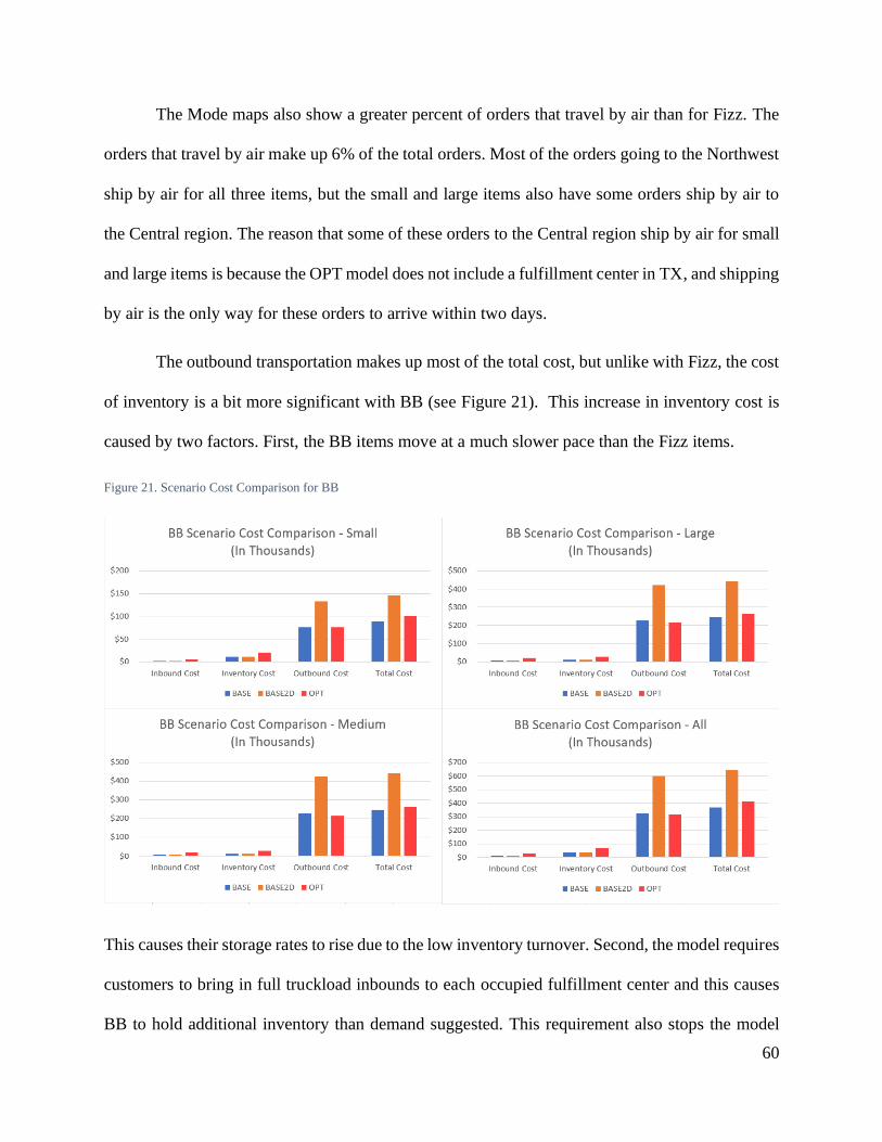
60
The Mode maps also show a greater percent of orders that travel by air than for Fizz. The
orders that travel by air make up 6% of the total orders. Most of the orders going to the Northwest
ship by air for all three items, but the small and large items also have some orders ship by air to
the Central region. The reason that some of these orders to the Central region ship by air for small
and large items is because the OPT model does not include a fulfillment center in TX, and shipping
by air is the only way for these orders to arrive within two days.
The outbound transportation makes up most of the total cost, but unlike with Fizz, the cost
of inventory is a bit more significant with BB (see Figure 21). This increase in inventory cost is
caused by two factors. First, the BB items move at a much slower pace than the Fizz items.
Figure 21. Scenario Cost Comparison for BB
This causes their storage rates to rise due to the low inventory turnover. Second, the model requires
customers to bring in full truckload inbounds to each occupied fulfillment center and this causes
BB to hold additional inventory than demand suggested. This requirement also stops the model

61
from selecting additional fulfillment centers even though the outbound would have been cheaper
by doing so. For example, the model opens a fulfillment center in TX for BB’s medium item, but
not for their small or large items due to the low volume. The GA fulfillment center does not open
for any of the solutions since it is cheaper overall to serve demand to the Southeast from PA (all
items originate out of NJ) at a higher on time performance for all three items.
The overall on-time percent for BB is 96% (see Figure 22). Orders fulfilled from PA and
IL have the highest on-time percent and are above the 95% threshold, while the on-time percent
for orders fulfilled from IL and TX are below the 95% threshold. GA has the lowest on-time
percent of all the fulfillment centers and is not selected for BB.
Even though BB currently fulfills all their orders from a single fulfillment center in PA,
they can deliver 62.2% of their orders within two days. This is because two-thirds of their demand
comes from the Northeast, Southeast, and Midwest regions. The only way BB could serve all their
customers within two-days in a cost-effective way is to add additional fulfillment centers,
otherwise one-third of their orders would need to be shipped by air. To make this transition to
100% two-day service fulfillment, BB can expect to pay an additional 74.6% moving from their
BASE scenario to the BASE2D scenario and an additional 11.5% moving from their BASE
scenario to the OPT scenario. Comparing the BASE2D scenario against the OPT scenario, BB
would save 36.1%.
62
Figure 22. On-time performance comparison for BB

63
4.2. Sensitivity Analysis
Uncertainty is an important component of the bidding process that SL runs when engaging with
new potential clients. Data such as demand profile, transportation rates and fulfillment policy
might not be fully available, and more importantly, might change over time.
For this reason, sensitivity analysis plays a key role in the deployment of the model we have
created. SL must estimate the ideal network design not only in “standard” conditions but should
understand how different factors can affect the optimal solution. We identify three elements of
uncertainty that can potentially change the optimal solution found by our model (summarized in
Table 15):
1. Changes in customer demand. Demand volume and demand variability impact the amount
of inventory that a company should carry. Key questions we address in this section are:
1.1. What if demand doubles or is cut in half?
1.2. What if demand variability increases?
2. Changes in the fulfillment policy. Customer expectations for fast deliveries are ever
increasing. The model is currently built to target delivery within 2 days, but it would be
interesting to understand the extra cost generated by faster delivery modes. The key question
to address is:
2.1. What if orders are fulfilled using a next-day window?
3. Changes in inbound transportation costs. The spot market for FTLs is volatile and rates vary
widely over time. The key question we address in this section is:
3.1. What if spot rates increase +10% or decrease -10%?

64
The sensitivity analysis is performed using BB as the test case, because, compared to Fizz, its cost
structure is more balanced in terms of relative magnitude of transportation vs. inventory cost.
Table 15. Sensitivity Analysis
Scenario # Change
Customer demand
1.1 Volume: 0.5x, 2x
1.2 Standard deviation: 2x, 3x
Fulfillment policy
2.1 Next day delivery
Inbound transportation
3.1 FTL Spot rates +/-10%
4.2.1. Changes in Customer Demand
Demand Volume. The total cost of the optimized network and the resulting network configuration
for two demand volume scenarios are included in Table 16.
Table 16. Sensitivity to demand volume
Costs (in thousands) Baseline (OPT) Demand Vol. = 0.5x Demand Vol. = 2x
Outbound Transp. $ 313 $ 171
(-45%)
$ 601
(+ 92%)
Inventory $ 67 $ 63
(-1%)
$ 77
(+14%)
Inbound Transp. $ 31 $ 17
(-45%)
$ 58
(+ 87%)
Tot Logistic Cost $ 411 $ 251 (-39%) $ 736 (+79%)

65
Fulfillment Centers
Open
Small: 3
Medium: 4
Large: 3
Small: 3
Medium: 4
Large: 3
Small: 4 (+1)
Medium: 5 (+1)
Large: 3
The scenario where demand volume is 0.5x the baseline is very similar to the current condition.
Besides the expected reduction in outbound and inbound transportation cost due to the smaller
volume of orders processed, the network configuration does not change in terms of fulfillment
center openings. The scenario is different when the volume doubles as one additional fulfillment
center is opened for both small and medium items. As more orders are processed, the outbound
transportation costs increase, causing the opening of more fulfillment centers to minimize the total
cost.
Demand Standard Deviation. A change in standard deviation of demand results in higher
inventory costs. When variability increases, each point of the inventory function moves up due to
two reasons. First, the amount of safety stock required to achieve a 98.5% service level gets larger.
Second, the non-linear structure of the fulfillment center rates changes the shape of the curve,
exacerbating the increase. Since more stock must be kept in the fulfillment center to reach the
desired level of service, inventory will turn less times per year, resulting in higher fulfillment
center rates (this is particularly true for Medium orders). The resulting inventory functions are
plotted in Figure 23.

66
Figure 23. Inventory Function with different variability scenarios
The results of the variability scenario are summarized in Table 17.
Table 17. Sensitivity to demand variability
Costs (in thousands) Baseline (OPT) Std dev = 2x Std dev = 3x
Outbound Transp. $ 313 $ 313
(+ 0%)
$ 326
(+ 4%)
Inventory $ 67 $ 95
(+ 42%)
$ 111
(+ 66%)
Inbound Transp. $ 31 $ 31
(+ 0%)
$ 32
(+ 3%)

67
Tot Logistic Cost $ 411 $ 439 (+7%) $ 469 (+14%)
Fulfillment Centers
Open
Small: 3
Medium: 4
Large: 3
Small: 3
Medium: 4
Large: 3
Small: 3
Medium: 3 (-1)
Large: 3
When the standard deviation of demand is 2x larger than the baseline, the optimal solution becomes
more expensive because due to the growth in inventory cost of 66%; however, the network
configuration remains substantially the same. There is no variation in outbound and inbound
transportation cost and the same fulfillment centers are opened. When the standard deviation is 3x
higher than the baseline, the network configuration changes. For medium items, three fulfillment
centers are opened instead of four as the gain of risk pooling is stronger in this scenario.
4.2.2. Changes in Fulfillment Policy
The current business goal for the majority of SL’s clients is to serve their end customers within
two days; however, a growing number of consumers demand even faster deliveries. For this reason,
an interesting scenario to assess is the added cost generated by using next day delivery services.
The results are included in Table 18.
Table 18. Sensitivity to fulfillment policy
Costs (in thousands) Baseline (OPT) Next Day Delivery
Outbound Transp. $ 313 $ 486 (+55%)
Inventory $ 67 $ 76 (+13%)
Inbound Transp. $ 31 $ 42 (+35%)
Tot Logistic Cost $ 411 $ 604 (+47%)

68
Fulfillment Centers
Open
Small: 3
Medium: 4
Large: 3
Small: 5 (+2)
Medium: 5 (+2)
Large: 3
Serving end-customers within the next day using the current network would increases the total
annual cost by 47%. This is due to the model being forced to ship air delivery for most of the
routes, causing outbound transportation cost to increase 55%. Moreover, the model suggests
opening more warehouse to be closer to the customer. For this reason, inventory costs increase
13% due to lack of risk pooling. Inbound transportation cost increases as well, because less
saturated FTL are used to supply the fulfillment centers.
Given the results of this scenario, it is evident that it will be hard for SL to offer next day delivery
services using the current network (five fulfillment centers) at a reasonable price. The
recommendation is to evaluate the activation of new fulfillment centers across the US, to be able
to reduce outbound transportation costs and use less air delivery.
4.2.3. Changes in Inbound Transportation Costs
Most clients of SL use spot rates for transporting goods from their own facilities to the fulfillment
centers. On a specific lane, spot rates are not constant throughout the year, but varies due to
demand-supply unbalance. Even though the total cost increases, a variation of +/-10% in the spot
rates does not change the optimal solution, as shown in Table 19. The reason for this is that inbound
transportation cost represents only a marginal portion of the total logistic costs (<10%).

69
Table 19. Sensitivity to inbound transportation costs
Costs (in thousands) Baseline (OPT) Spot rates = -10% Spot rates = +10%
Outbound Transp. $ 313 $ 313 $ 313
Inventory $ 67 $ 67 $ 67
Inbound Transp. $ 31 $ 28 (-10%) $ 34 (+10%)
Tot Logistic Cost $ 411 $ 408 (-0.7%) $ 414 (+0.7%)
Fulfillment Centers
Open
Small: 3
Medium: 4
Large: 3
Small: 3
Medium: 4
Large: 3
Small: 3
Medium: 4
Large: 3
70
5. Conclusion
A centralized supply chain network with fewer warehouses offers potential savings in inventory
costs due to the risk pooling effect. On the other end, such network configuration tends to increase
the outbound transportation cost. In the e-commerce space, where delivery speed is a key success
factor, this increase in transportation costs is exacerbated.
In this research, we developed a mixed integer linear model to design a supply chain network
that optimally balances the trade-off between the inventory savings realized by a centralized
network and the transportation costs efficiencies achieved by a decentralized configuration. The
right balance between these two conflicting objectives has to be found while specific business
targets are met, such as fast delivery service (within two-days) and on-time performance of at least
95%.
The model has been validated for two different clients of SL and has proven to bring benefits
for companies looking to serve their customers within two days. In the case of Fizz, a beverage
company, our model recommends that they use five fulfillment centers (instead of their current
number of three) and that they would save 8.4%. Given the nature of the product (high density),
the model suggests using a fully decentralized network (5 fulfillment centers activated) because
transportation costs are much more impactful than inventory costs. In the case of BB, a bakery
goods company who currently uses one fulfillment center, our model recommends that they use
three and four fulfillment centers (depending on the order size) and that they would save 36.1%.
The reason for this recommendation is due to the high cost that BB needs to pay to serve their
customers nationwide within two days from a single fulfillment center. By having additional
fulfillment centers, BB can serve all their customers in a cost-effective way.

71
We ran an additional layer of validation by testing the sensitivity of our model to changes in
customer demand, inbound transportation modes, and fulfillment strategies. The sensitivity is
particularly important to SL because our model will be run during the pre-sales process when
information on the client business might be not always accurate. The model has reacted well to
this validation and results are consistent and stable across the various scenarios.
Various improvements can be implemented by the SL to expand the model developed in this
research. First, having a time-phased network configuration might bring potential benefits when
dealing with highly seasonal products. Second, in the case that SL might consider opening new
fulfillment centers to support their growing B2C e-commerce business, our model could be used
to support this strategic decision with a slight modification of the objective function. Third, the
model assumes that the risk pooling effect follows a square root law. However, client-specific
inventory function might be estimated with simulation and plugged into our optimization model.
Fourth, SL may add more carriers and modes as inputs to the model and exploit the optimization
engine to evaluate the benefit of having those delivery options in its portfolio.

72
References
Bertsimas, D., & Tsitsiklis, J. N. (1997). Introduction to linear optimization (Vol. 6, p. 196).
Belmont, MA: Athena Scientific.
Burgin, T. A. (1975). The gamma distribution and inventory control. Journal of the Operational
Research Society, 26(3), 507-525.
Consumer Intelligence Research Partners. (2020). US Amazon Prime Members – Slow, Steady
Growth. https://files.constantcontact.com/150f9af2201/9f9e47b4-0d66-4366-ad76-
552ae3daa4f0.pdf
Croxton, K. L., Gendron, B., & Magnanti, T. L. (2003). A Comparison of Mixed-Integer
Programming Models for Nonconvex Piecewise Linear Cost Minimization Problems.
Management Science, 49(9), 1268–1273.
Croxton, K. L., & Zinn, W. (2005). Inventory Considerations in Network Design. Journal of
Business Logistics, 26(1), 149–168.
CVS Pharmacy. (2020, October 08). CVS/Pharmacy Routing Guide.
https://cvssuppliers.com/sites/default/files/CVS%20Routing%20Guide%20Instructions%
20-%20version%2067.pdf
Daskin, M. S., Coullard, C. R., & Shen, Z. J. M. (2002). An inventory-location model:
Formulation, solution algorithm and computational results. Annals of operations research,
110(1-4), 83-106.
73
Eskigun, E., Uzsoy, R., Preckel, P. V., Beaujon, G., Krishnan, S., & Tew, J. D. (2007). Outbound
supply chain network design with mode selection and lead time considerations. Naval
Research Logistics (NRL), 54(3), 282-300.
Fareeduddin, M., Hassan, A., Syed, M. N., & Selim, S. Z. (2015). The impact of carbon policies
on closed-loop supply chain network design. Procedia CIRP, 26(Complete), 335-340.
FedEx. (2020). Coronavirus. https://www.fedex.com/en-us/coronavirus.html
Jayaraman, V. (1998). Transportation, facility location and inventory issues in distribution network
design. International Journal of Operations & Production Management.
Maister, D. H. (1976). Centralization of inventories and the “square root law”. International
Journal of Physical Distribution, 6(3), 124-134.
Melo, M. T., Nickel, S., & Saldanha-Da-Gama, F. (2009). Facility location and supply chain
management–A review. European journal of operational research, 196(2), 401-412
Nahmias, S., & Olsen, T. L. (2015). Production and Operations Analysis (7th ed.).
Waveland Press.
National Retail Federation. (2019). 2018/2019 Winter Consumer View.
https://cdn.nrf.com/sites/default/files/2019-01/Consumer%20View%20Winter%202018-
2019_0.pdf
Panko, R. (2019, September 4). How Consumer Hunger for Two-Day Delivery Impacts Small
Businesses. Clutch. https://clutch.co/logistics/resources/how-two-day-delivery-impacts-
small-businesses

74
Schmitt, A. J., Sun, S. A., Snyder, L. V., & Shen, Z. J. M. (2015). Centralization versus
decentralization: Risk pooling, risk diversification, and supply chain disruptions. Omega,
52, 201-212
Shapiro, J. (2006). Modeling the Supply Chain. Nelson Education.
Silver, E. A., & Peterson, R. (1985). Decision systems for inventory management and production
planning. John Wiley & Sons Incorporated.
UPS. (2020). Billable Weight. https://www.ups.com/us/en/help-center/packaging-and-
supplies/determine-billable-weight.page
You, F., & Grossmann, I. E. (2008). Mixed-Integer Nonlinear Programming Models and
Algorithms for Large-Scale Supply Chain Design with Stochastic Inventory Management.
Industrial & Engineering Chemistry Research, 47(20), 7802–7817.
Yu, Y., Wang, X., Zhong, R. Y., & Huang, G. Q. (2016). E-commerce Logistics in Supply Chain
Management: Practice Perspective. Procedia CIRP, 52, 179–185.
Watson, M., Lewis, S., Cacioppi, P., & Jayaraman, J. (2013). Supply chain network design:
applying optimization and analytics to the global supply chain. Pearson Education.