network layer - cs.virginia.edujorg/teaching/cs457/slides/network.pdf · 1 © jörg liebeherr,...

1

© Jörg Liebeherr, 1998,1999 CS457

Network Layer

Introduction Datagrams and Virtual Circuits

RoutingTraffic Control


Introduction

• Main Task of the network layer is to move packets from the source host to the destination host

• Lowest layer to deal with end-to-end issues!

Transport

Session

Presentation

ApplicationTransport

Session

Presentation

Application

Physical

Data Link

Network

Physical

Data Link

Network

Physical

Data Link

Network

Physical

Data Link

Network

Physical

Data Link

Network

Physical

Data Link

Network

Station (Host)

Node (Router)

2


Issues at the Network Layer

• Switching Technique:

– Datagrams

– Virtual circuits

• Routing:

– How to forward packets

– How to calculate a path from source to destination?

• Traffic Control:

– Congestion control

– Rate control


Issues at the Network Layer

• Naming and Addressing:

– How to find the name of a network node?

• Internetworking:

– How to interconnect heterogeneous networks?

3


Services and Implementation

• 2 packet switching techniques are used:

– Datagrams

– Virtual Circuits

• 2 services are provided to the transport layer:

– Connectionless Service– Sender and receiver treat each transmitted message as an

independent unit

– Connection-oriented Service– Sender and receiver see data as traveling on a logical

connection

– Receiver receives data in the same order in which they are transmitted


Connectionless and Connection-oriented

• Connectionless service and connection-oriented service can be reliable or unreliable

Reliable = Delivery of all data is ensured. The receiver acknowledges data and sender retransmits data that was not received

Unreliable = No acknowledgments or retransmission of data

• Note: unreliable connectionless service is often called “datagram service”

4


Datagram Packet-Switching

• Each packet is routed independently

A 1

2 3

6

54

B

C

2 1

2

1

33


Virtual-Circuit Packet Switching

• All packets of a VC follow the same route

A 1

2 3

6

54

B

C

VC #1

VC #2

5


Connectionless Service

• Each packet is transmitted independently

Packet-switchednetwork

B.3 B.2 B.1

C.3 C.2 C.1

B.2B.3

B.1

C.1C.2

C.3

A

B

C


Connection-oriented Service

• Logical connection is established

Packet-switchednetwork

1.3 1.2 1.1

2.3 2.2 2.1

1.31.2

1.1

2.32.2

2.1

A

B

C

6


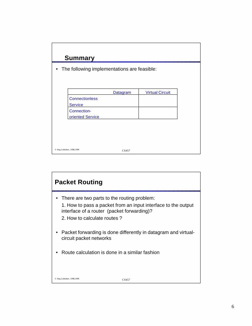
Datagram Virtual Circuit

Connectionless

Service

Connection-

oriented Service

Summary

• The following implementations are feasible:


Packet Routing

• There are two parts to the routing problem:

1. How to pass a packet from an input interface to the output interface of a router (packet forwarding)?

2. How to calculate routes ?

• Packet forwarding is done differently in datagram and virtual-circuit packet networks

• Route calculation is done in a similar fashion

7


Packet Forwarding of Datagrams

• Recall: In datagram networks, each packet carries the full destination address

• Each router maintains a routing table which has one row for each possible destination address

to

x

w v n

n

via(next hop)

d

Routing Table of node v

d


Packet Forwarding of Datagrams

• When a packet with destination node arrives at an incoming link, ...

1. The router looks up the routing table

2. The routing table lookup yields the address of the next node (next hop)

3. The packet is transmitted onto the outgoing link that goes to the next hop

Good: The router does not need to know about end-to-end flows

Bad: Size of the routing table can grow very large

8


Packet Forwarding with Virtual Circuits

• Recall: In VC networks, the route is setup in the connection establishment phase

• During the setup, each router assigns a VC number (VC#) to the virtual circuit

• The VC# can be different for each hop• VC# is written into the packet headers

3vx

w v n

2w

Routing Table of node v

dfrom VC# to VC#

path of virtualcircuit

2 31


Packet Forwarding of Virtual Circuits

• When a packet with VCin in header arrives from router n in, ...

1. The router looks up the routing table for an entry with (VCin, nin)

2. The routing table lookup yields (VCout, nout)

3.The router updates the VC# of the header to VCout and transmits the packet to nout

Good: Routing table is small (how small?)

Bad: Changing the route is complicated

Routing table changes for each virtual circuit

9


Comparison

Issue Datagram Network Virtual CircuitNetwork

Circuti Setup Not needed Required

Addressing Each packet containsthe full source anddestination address

Each packet containsonly a VC number

StateInformation

Network does not holdstate information onflows

Each VC is stored inthe network

Routing Each packet is routedindependently

Route chosen whenVC is setup. Allpackets follow sameroute

Effect ofrouter failure

Some packets are lost All VCs at crashedrouter are terminated

CongestionControl

Difficult Easier (but notsimple)


Routing Algorithms

• Objective of routing algorithms is to calculate `good’ routes

• Routing algorithms for both datagrams and virtual circuits should satisfy:

- Correctness - Simplicity

- Simplicity - Robustness

- Stability - Fairness

- Optimality

• Impossible to satisfy everything at the same time

10


Fairness vs. maximum throughput

• Example: Assume that stations A, B, C wants to send to A’, B’, and C’, each at 5 Mb/s

• Assume the capacity of the network links is 10 Mb/s.

D D’

A

A’

B

B’

C

C’


Stability vs. optimal delay

• Example: Optimize delay by sending all packets over link with the least traffic.

– Update the routing decision every 10 sec

A

B

C

D

96 Kbps

11


Elements of Routing Algorithms

• Optimization Criteria:

- Number of Hops - “Cost”

- Delay - Throughput

• Decision Time:

– Once per session (VCs)

– Once per packet (datagram)

• Decision Place:

– Each node (distributed routing)

– Central node (centralized routing)

– Sending node (source routing)


Shortest-Path Routing

• Adaptive routing algorithms use a shortest path algorithm to calculate the route with the least cost

• Three components:

1. Measurement Component

• Nodes (routers) measure the current characteristics such as delay, throughput, and “cost”

2. Protocol

• Nodes disseminate the measured information to other nodes

3. Calculation

• Nodes run a least-cost routing algorithm to recalculate their routes

12


Goal of Shortest Path Routing

• Goal: Given a network were each link between two nodes i and j is assigned a cost. Find the path with the least cost between nodes i and j.

• Parameters:

dij cost of link between node i and node j;

dij = ∞, if nodes i and j are not connected;dii = 0

N set of nodes


Approaches to Shortest Path Routing

• There are two basic approaches to least-cost routing in a communication network

• There are two basic approaches to shortest-path routing:

1. Link State Routing

2. Distance Vector Routing

13


Approaches to Shortest Path Routing

• 1. Link State Routing – Each node knows the distance to its neighbors

– The distance information (=link state) is broadcast to all nodes in the network

– Each node calculates the routing tables independently

2. Distance Vector Routing– Each node knows the distance (=cost) to its directly

connected neighbors

– A node sends a list to its neighbors with the current distances to all nodes

– If all nodes update their distances, the routing tables eventually converge


Link State Routing

• Each node must

– discover its neighbors

– measure the delay (=cost) to its neighbors

– broadcast a packet with this information to all other nodes

– compute the shortest paths to every other router

• The broadcast can be accomplished by flooding

• The shortest paths can be computer with Dijkstra’s algorithm

14


Dijkstra’s Algorithm

• Finds the shortest path from a source node to all other nodess source node

Dn cost of the least-cost path from node s to node n

M = {s};for each n ∉∉ M

Dn = dsn;while (M ≠≠ all nodes) do

Find w ∉∉ M for which Dw = min{Dj ; j ∉∉ M};Add w to M;for each n ∉∉ M Dn = minw [ Dn, Dw + dwn ];Update route;

enddo


Example Network

11

22 33

44 55

66

5

2

1

1

1

2

23

35

15


Example

• Example: Calculate the shortest paths for node 1.

Iteration M D1 D2 D3 D4 D5 D6

Init


Example

• Result is a routing tree:

... which results in a routing table (of node 1):

16


Discussion of Link State Routing

• Recall: Link State Routing methods use Dijkstra's algorithm

• Each node requires complete topology information

• Each node has two tasks:

– Test status of all neighbor nodes

– Propagate link state information of neighbors to all other nodes by sending a broadcast message

• Whenever a link state message arrives.…

• the node updates its topology information

• and recalculates the shortest paths


Discussion of Link State Routing

• Advantages of Link State Routing:

– Each nodes computes routes from the same data

– Guaranteed to converge

– Update messages (state information) does not depend on total number of nodes; only depends on number of neighbors

• Disadvantages of Link State Routing:

– Each node must maintain global database

17


Distance Vector

• Each node maintains two tables:

– Distance Table: Cost to each node via each outgoing link

– Routing Table: Minimum cost to each node and next hop node

• Nodes exchange messages that contain information on the cost of a route

• Reception of messages triggers recalculation of routing table


Distance Vector Algorithm: Tables

l (v,w) cost of link (w,v)C d(v,w) cost from v to d via wDd(v) minimum cost from v to d

to

Cd(v,n)C

d(v,w)

nw

n

v w dl(v,w)

d

viato

Dd(v)n

costvia(next hop)

d

Distance Table RoutingTable

Note: In the figure, Cd(v,w)<Cd(v,n) and, therefore, Dd(v) = Cd(v,n)

18


Messages

• Nodes exchange messages to their neighbors.

• If node v sends a messages to node x of the form, [m , Dm (v)], this means

“I can go to node m with minimum cost Dm (v)”

vv xx

This message is only of interest to neighbors of v

[m , Dm (v)]


New link with cost l(m,v) comes up

to

l(m,v)Cm(v,p)

mp

n

v w dl(v,w)

m

viato

Dm(v)n

costvia(next hop)

m


ml(m,v)

New column

New row

19


New link with cost l(m,v) comes up

Operations at node v1. Add new row in distance and routing table, and new column to

distance table

2. Recalculate distance table under consideration of l(m,v)

3. Compute minw Cm(v,w):

(a) If no changes to previous value of minw Cm(v,w): Do nothing

(b) If Cm(v, m) = minw Cm(v,w)Dm(v)=Cm(v,m) change entry in m-th row of routing table to (m, , Dm(v)) and send message [m, Dm(v)] to all neighbors

3. Also: Since v is a neighbor of m, v sends the contents of its

routing table to m: [a, Da(v)], [b, Db(v)], ...., [z, Dz(v)]


Cost of link changes by ∆∆m

e

tom

v d

d

viato

Dd(v)m

costvia(next hop)

d


ml(m,v)+∆m

e

Ce(v,m)+∆ m

Cd(v,m)+∆ m

y

x

De(v)ye

20


Cost of link changes by ∆∆m

Operations at node v

1. Entries in m-th column of distance table are changed by ∆ (if link goes down: ∆ = ∞).

2. For all destinations d:

Compute minw Cm(v,w):

(a) If no changes to previous value of minw Cm(v,w): Do nothing

(b) If Cm(v, m) = minw Cm(v,w)Change entry in d-th row of routing table to (m,Cd(v, m)), and send messages [d, Cd(v, m)] to all neighbors


Node v receives a message [d, Dd(w)]

to

Cd(v,w)

w

w v[d,D

d(w)]

d

viato

Dd(v)j

costvia(next hop)

d


21


Node v receives a message [d, Dd(w)]

Operations at node v1. If d = v then ignore the message2. If d ≠ v then

Cd(v, w) = Dd(w) + l (w,v)

Compute minx Cd(v,x) :

If no changes, then do nothing

If Cd(v,w)=minx Cd(v,x), thenchange entry in d-th row of routing table to (d, Cd(v, w)) and send message [d, Cd(v,w)] to all neighbors.


Example

• Assume that Node 1 comes up at time t=0

• Show how the entries for destination 1 are updated at all other nodes

11

22 33

44 55

66

5

2

1

1

12

23

35

22


Example

v ia cos tv i a 1 3 4

Node 2

Dis tance Rout ing

v ia cos tv i a 1 2 4 5 6

D is tance Rout ing

Node 3

v ia costv i a 1 2 3 5

Node 4

via costvia 3 4 6

Node 5

Distance Routingvia costvia 5 6

Distance Routing

Node 6

1

2 3

4 5

6

5

2

12

3

3

1

1

2

5


Discussion of Distance Vector Routing

• Entries of routing tables can change while a packet is being transmitted. This can lead to a single datagram visiting the same node more than once (Looping)

• If the period for updating the routing tables is too short, routing table entries are changed before convergence (from the previous updates) is achieved

• Example: The ARPANET used a Distance Vector algorithm with an update period of <1 sec. Due to the instability of routing, the ARPANET switched in 1979 to a link state routing algorithm

23


Routing Algorithms in the Internet

Distance Vector

• Routing Information Protocol (RIP)

• Gateway-to-Gateway Protocol (GGP)

• Exterior Gateway Protocol (EGP)

Link State

• Intermediate System -Intermediate System (IS-IS)

• Open Shortest Path First (OSPF)


Traffic Control

• Traffic control at the network layers attempts to control the number of packets that are in the network at a time

• Goal of traffic control:Prevent the network from becoming a bottleneck

• Different types of traffic control:

– Flow Control

– Congestion Control

– Routing

24


Flow Control vs. Congestion Control

• Flow Control - regulates the rate of the data flow between two points

• Congestion Control - regulates the number of packets that can be in the network

• Congestion control may consider more than two points, i.e., it may deal with the entire network.


What is Congestion ?

• Congestion occurs if the number of queued packets at the output buffers of a router grows large

• Effect of long queues in output buffers: increased delays, buffer overflows, timeouts at sender, etc

Router

Output buffer

25


When does Congestion Occur ?

• Define the Offered Load of a network to be the average rate of packets that enter the output queue

• The following are pretty good rules of thumb:

– Average number of packets in queue =

– Average delay in output queue =Load

Load−1

Load−11


Effects of Congestion

• Congestion occurs if Load → 1

Load

Delay1 ideal

controlled

uncontrolled

1

Throughput1 ideal

controlled

uncontrolled

1Load

26


Problems without Traffic Control

• The following problems may occur in a network with insufficient traffic control at the network layer.

– Loss of Efficiency

– Unfairness

– Lockup (Deadlock)


Loss of Efficiency

• Throughput may decrease if offered load is increased

Throughput1 ideal

controlled

uncontrolled

1Load

27


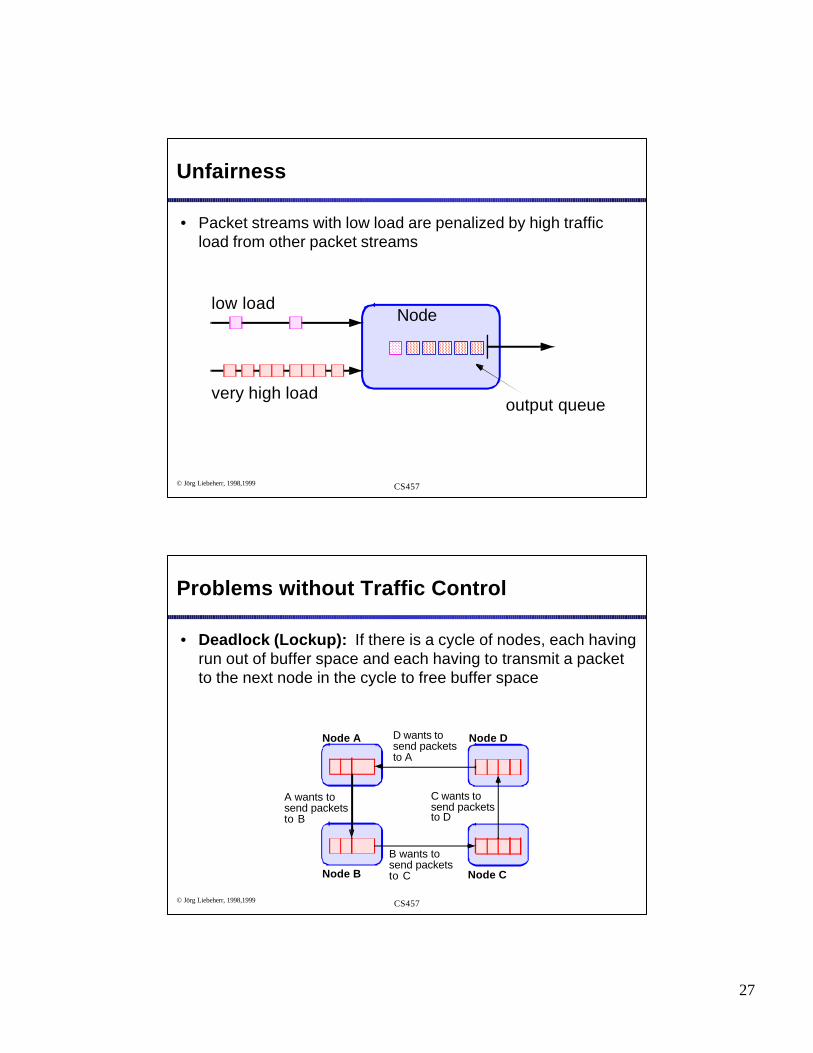
Unfairness

• Packet streams with low load are penalized by high traffic load from other packet streams

output queue

Nodelow load

very high load


Problems without Traffic Control

• Deadlock (Lockup): If there is a cycle of nodes, each having run out of buffer space and each having to transmit a packet to the next node in the cycle to free buffer space

Node A Node D

Node B Node C

A wants to send packetsto B

B wants tosend packetsto C

C wants to send packetsto D

D wants to send packetsto A

28


Scope and Level of Traffic Control

• Traffic Control can be done at several levels:

Station StationNode NodeNode

DataLink

Net-work

Trans-port

End-to-End Level

Entry-to-Exit level

NetworkAccess

Network Access

HopLevel

HopLevel

HopLevel

HopLevel

NetworkAccess

NetworkAccess


Techniques for Traffic Control

• Preallocation of Buffers

• Packet Discarding

• Choke Packets

• Sliding Window Flow Control

• Leaky Bucket

29


Preallocation of Buffers

• Approach: Reserve sufficient buffer space at each node for each virtual circuit during the virtual circuit setup phase

• Requires admission control: If sufficient buffers are not available, reject the virtual circuit

• Caveat: Overallocation of buffer space will limit the utilization of the network.


Packet Discarding

• Drop packets if they arrive at a node with almost full buffers

• Heuristics should be used to decide when to drop a packet

• For example, ACK packets should not be dropped

30


Choke Packets

• If a packet enters a node and the queue length of the outgoing buffer exceeds a threshold, the node sends a choke packet to the source node

• If the source node receives a choke packet it reduces the traffic by a certain amount.

• For example, the window size could be reduced.

– If a (throttled) source node does not receive a choke packet within a given time interval, it is allowed to increase the traffic.

• Example: IP (Internet Protocol) uses choke packets


Sliding Window Flow Control

• Can be used at the hop-by-hop and the entry-to-exit level

31


Leaky Bucket

• A Leaky Bucket is used to control the maximum rate at which a sender can transmit traffic

• Leaky buckets operate at the station/node interface

• Two parameters: token rate r and bucket size B

Network

packetarrivals

packet queue

new tokens

TokenBucket

r

B


Operation of a Leaky Bucket

• Tokens are added to the token bucket at rate of r

• No tokens are added to the token bucket if the bucket contains already B tokens

• For each transmitted packet tokens must be removed from the bucket (one token per for each byte)

• If the token bucket does not have enough tokens, the packet is either dropped

• (In some versions of the leaky buckets the packets can be queued until a token arrives)

network layer - cs.virginia.edujorg/teaching/cs457/slides/network.pdf · 1 © jörg liebeherr,...

Documents