network routing and unreliable communication link compensation555779/fulltext01.pdf · network...

Implementation of a Wireless Control System

Network Routing and Unreliable Communication Link Compensation

JAKOB WALLANDER

Master’s Degree Project in

Automatic Control

Stockholm, Sweden 2012

XR-EE-RT 2012:016

Abstract

Wireless communication systems have been a part of everyday life for manydecades but implemented in an industrial control system they are yet tomake their big breakthrough. This is despite of the fact that wireless controlsystems show great promise in reducing installation costs and down time.The biggest reason why they have not already revolutionised the industry isreliability, as they are much more susceptible to delays and communicationbreakdowns compared to their wired counterpart.

The foundation for this thesis is the following scenario. In an industrya control loop uses a wireless link between the control computer and theactuator. A forklift moving heavy equipment happens to park in a positionwhere it is blocking the communications. This thesis suggests a solution tothis problem through the implementation of two separate measures. Firsta Collection Tree routing Protocol (CTP) is responsible for detecting bro-ken links and finding a disturbance free path for the packet through thenetwork. Secondly a Kalman filter based Predictive Outage Compensator(POC) estimates the missing data when the real control signal is delayed ormissing.

In the implementation the Moteiv Tmote Sky was used for the networknodes and the double tank process as test bed for the POC. The resultsshow that the CTP network is capable of routing the data through multiplehops without too much delay and that between 1 and 8 packets are lostduring route changes. The POC performs on average 8 % better than themore common and naive solution to simply hold the most recently receivedvalue in case of outage.

i

Sammanfattning

Tradlosa kommunikationssystem har varit en del av vardagen i manga de-cennier, men i industriella styrsystem vantar de fortfarande pa sitt storagenombrott. Detta trots att tradlosa styrsystem visar pa lovande mojligheteratt kunna minska installationskostnader och stop i processerna. Den storaanledningen till att de inte redan har revolutionerat branschen ar tillforlit-ligheten. De ar avsevart mer mottagliga for fordrojningar och kommunika-tionshaverier jamfort med en tradbunden motsvarighet.

Denna avhandling har sin grund i foljande scenario. I en industri finnsett reglersystem som anvander sig av en tradlos lank mellan styrdatorn ochstalldonet. En gaffeltruck som flyttar tung utrustning i fabriken rakar park-era i ett lage dar den blockerar kommunikationen. Avhandlingen foreslaren losning pa detta problem genom tva separata atgarder. Forst genomimplementationen av ett Collection Tree Protocol (CTP) som ansvarar foratt upptacka trasiga lankar och att hitta en vag for paketeten som ar frifran avbrott. I andra hand genom en Kalmanfilterbaserad Predictiv OutageCompensator (POC) som har till uppgift att skatta styrsignalen da verkligadata ar forsenade eller saknas.

For implementationen anvandes Moteiv Tmote Sky i alla natverksnoderoch tva-tanks processen som testplattform for POCen. Resultaten visaratt CTP natverket klarade att dirigera data genom flera hopp utan alltforstora drojsmal och att mellan 1 och 8 paket tappas da topografin i natetandras. POCen var i allmanhet 8% battre pa att bibehalla kontrollpre-standan vid natverksavbrott an den enklare losningen att halla det senastestyrsignalsvardet om inget nytt kommer.

iii

NOMENCLATURE

Notations

E[w] Expected value of w

V ar(w) Variance of w

x+ Next discrete value of x

x− Previous discrete value of x

Variables

u Estimated control signal/pump voltage . . . . . . . . . . . . V

r Reference for lower tank . . . . . . . . . . . . . . . . . . . . . m

u Control signal/pump voltage . . . . . . . . . . . . . . . . . . V

x1 Water level upper tank . . . . . . . . . . . . . . . . . . . . . m

x2 Water level lower tank . . . . . . . . . . . . . . . . . . . . . . m

Abbreviations

CSMA Carrier Sense Multiple Access

CTP Collection Tree Protocol

ETX Expected transmission

IAE Integrated Absolute Error

LTI Linear Time-Invariant system

OSI Open Systems Interconnection

POC Predictive Outage Compensator

TDMA Time Division Multiple Access

UPM Universal Power Module

v

CONTENTS

Abstract i

Sammanfattning iii

Nomenclature v

Contents vii

1 Introduction 11.1 Wireless Control . . . . . . . . . . . . . . . . . . . . . . . . . 11.2 Problem Formulation . . . . . . . . . . . . . . . . . . . . . . . 21.3 Outline . . . . . . . . . . . . . . . . . . . . . . . . . . . . . . 3

2 Packet Routing in a Multi-Hop Network 52.1 Program Abstraction Layers . . . . . . . . . . . . . . . . . . . 52.2 The CTP Algorithm . . . . . . . . . . . . . . . . . . . . . . . 6

3 Compensating for Lost Packets 113.1 Introduction . . . . . . . . . . . . . . . . . . . . . . . . . . . . 113.2 The Closed Loop System . . . . . . . . . . . . . . . . . . . . . 123.3 Outage Compensation . . . . . . . . . . . . . . . . . . . . . . 13

4 Implementation 174.1 The Tmote Sky . . . . . . . . . . . . . . . . . . . . . . . . . . 174.2 The Double Tank Process . . . . . . . . . . . . . . . . . . . . 184.3 Implementation of a Small CTP Network . . . . . . . . . . . 214.4 The Kalman Based POC . . . . . . . . . . . . . . . . . . . . . 22

5 Results 255.1 Evaluation of CTP Routing Performance . . . . . . . . . . . . 255.2 Simulation of POC Performance . . . . . . . . . . . . . . . . 295.3 Implemented POC Experiments . . . . . . . . . . . . . . . . . 36

6 Conclusions 396.1 Future Work . . . . . . . . . . . . . . . . . . . . . . . . . . . 39

Bibliography 41

vii

CHAPTER

1

INTRODUCTION

Wireless communication has become a more and more important part ofthe modern society. Different technical solutions ranging from the infra-redshort range system in a TV remote control, to ultrasonic signals and radiofrequency communication systems. All of the above systems aim to solvethe problem of transporting information from one device to another withouthaving to connect them with cables[1].

Today we depend on wireless systems in many parts of our daily lives.They are used for distributing information through TV, radio and internet,for communication with cellular telephones and different radio systems, forpositioning in the Global Positioning System and much more. In the indus-try wireless systems are already widely used for monitoring processes andgathering data and in the future they are expected to play an importantrole in the control of industrial processes. This thesis investigates how sucha control system could be constructed.

In this chapter the reader is given an introduction to wireless communi-cations from a control theory point of view and the problems to be solvedare presented. Finally the Chapter contains the outline of the rest of thereport.

1.1 Wireless Control

In basically all industries there is a desire to control different processes.All control theory is based on the idea of continuously measuring states of asystem and then calculate how to actuate in order to achieve desired output.It does not matter if it is the temperature in an oven, the speed of a conveyorbelt or the water level in a coolant tank.

In most industrial applications several sensors have been built in to theprocess at the time of construction. These sensors transmit data through awired sensor network to a central control computer. The computer performsall calculations in real time and sends control signals through another setof wires to an actuator unit that outputs for example voltage to motors,

1

Introduction

valves, heater elements etc. The use of cables for transmitting data hasseveral drawbacks. First of all it creates a system with limited flexibility. Itis hard to move equipment and sensors that are connected with cables andif the process needs to be upgraded with more sensors new cables have tobe installed. This leads to a second drawback with wired control systems.It is extremely expensive to install new cables in an already operationalindustry. There are strict limitations on where cables can be installed andthe production might have to be shut down during the work, leading to bigfinancial losses. With a wireless network, equipment can be moved and newsensors installed to improve the process with relative ease. Also, wirelessnetworks are less susceptible to ware and tare and can therefore save moneyby reducing maintenance and downtime[2, p. 2].

The downside of wireless communication is that it is less reliable. In anindustrial environment especially, there are many uncontrollable things thataffect radio communications. This introduces uncertainties into the controlsystem such as transmission delays, lost packets or even complete communi-cation breakdown between nodes. To achieve good performance these uncer-tainties needs to be taken into account and compensated for when designingthe wireless network and controller. Furthermore the capacity limitations ina wireless network are more complex than in a wired counterpart. Differentsignals needs to be separated in time, frequency or location, meaning thattwo nodes can not transmit data on the same channel at the same time ifthey are within range of each other.

All in all it is clear that wireless communications will become a centralpart of future control systems just as they will create many opportunities toimprove on existing ones.

1.2 Problem Formulation

The problem considered in this master thesis is how to construct a simplifiedversion of a wireless control system that could be used in an industrialenvironment.

The final system as shown in Figure 1.1 has to be able to handle heavydisturbances to the radio communication between individual nodes in thenetwork and re-route control traffic through links that are disturbance free.The report will describe how this network routing can be achieved by usingthe Collection Tree Protocol (CTP) algorithm.

A strategy to cope with lost packets caused by imperfections in thenetwork routing has to be a part of the control method. This report willsuggest a solution where a model based Predictive Outage Compensator(POC) is used on the receiver side of the network to fill in the informationneeded when packets are lost.

Finally the control system is implemented on the classic double-tank pro-cess described in Section 4.2, using the Moteiv Tmote Sky motes describedin Section 4.1 for the network nodes.

This thesis’s focus is on the actuator side of the system, shown in black inFigure 1.1. The CTP network is implemented between the controller and the

2

1.3. Outline

POCController

Network

POC Process

Network

Figure 1.1: Overview of the wireless control system.

actuator while communications between the sensor and the controller (shownin gray in the Figure) is considered to be ideal. The POC is implemented asa part of the actuator. For further reading on the sensor side of the systemplease refer to master thesis by Ivar Cornell [3].

1.3 Outline

The outline of the rest of this thesis is as follows.

• The theory behind the CTP algorithm is presented in Chapter 2.

• Chapter 3 explains the stochastically synthesized POC, also referredto as the Kalman based POC, for the general case.

• The thesis continues with the implementations in Chapter 4, wherethe Tmote Sky is presented as well as the double tank process and thederivation of its model. The Chapter also describes how the CTP isimplemented to create a small network and how a Kalman based POCfor the double tank system is calculated.

• Chapter 5 contains results, first from experiments on the CTP networkand then from simulations of the outage compensators. Experimentaldata from the real double tank system with the CTP network andcompensators implemented is also presented.

• Finally in Chapter 6, conclusions are drawn and interesting areas offuture work are presented.

3

CHAPTER

2

PACKET ROUTING IN AMULTI-HOP NETWORK

Packet routing attempts to solve the problem of sending data through anetwork along a varying path while minimizing delays and losses. Manydifferent routing techniques have been developed over the years and thisthesis will focus on one technique in particular that is widely regarded as areference protocol for data collection, the Collection Tree Protocol (CTP).

The following Sections first include a short introduction to some of thecomponents that constitute a wireless network. This knowledge is needed tofully understand the CTP routing algorithm that is the main topic of thisChapter. For information on how a CTP network can be implemented usingTinyOS, please refer to Section 4.3.

2.1 Program Abstraction Layers

The goal of this Section is to give a very short introduction to the OpenSystems Interconnection (OSI) model and pinpoint the areas that are ofinterest for the rest of this thesis. The OSI model in Figure 2.1 is a goodway to visualize how a communication system works by dividing the programup into seven different layers. A brief explanation of the layers is availablebelow[4].

• Application layer.The application layer is closest to the user and interacts directly withfor example control algorithms.

• Presentation layer.The presentation layer works as a translator between the applicationand the other network levels and as such allows higher level applica-tions to use different syntax and semantics. The presentation layer isnot discussed further in this thesis.

5

Packet Routing in a Multi-Hop Network

Physical

Datalink

(MAC)

Network

(Routing)

Transport

Session

Presentation

Application

Recieving data

Sending data

Figure 2.1: The OSI network stack.

• Session layer.The session layer controls connections between nodes. It manages theconnection between the local and remote application. The session layeris not a part of this application and will not be discussed further.

• Transport layer.The transportation layer ensures end to end delivery of packets in anetwork. It is not active in this application and will not be discussedfurther.

• Network layer.Also referred to as routing layer. The network layer controls the flowof data in the network and the Collection Tree Protocol investigatedin this thesis is implemented as a part of it.

• Data link layer.Also referred to as MAC layer. Simultaneous communication betweennodes is avoided in this layer. There are different solutions for this.The Time Division Multiple Access (TDMA) schedule is a contention-free MAC that distributes timeslots to nodes statically or dynamically.Another example is the contention-based Carrier Sense Multiple Ac-cess (CSMA) MAC used for this implementation. The CSMA MACimplements no fixed schedule, instead the individual nodes sense thechannel to make sure it is free before sending packets.

• Physical layer.The physical layer is closely connected to the hardware. It takes care ofthe final output to, or first input from, different transmission mediumssuch as copper cables or the air, in case of radio communications.

2.2 The CTP Algorithm

The Collection Tree Protocol is a tree-based collection protocol, meaningthat all communications is passed down a tree structure of nodes and col-lected in one or several roots as in Figure 2.2[5, 6].

6

2.2. The CTP Algorithm

S1 S2 S3 S4

S5 S6 S7

S9S8 S10

Root 1 Root 2

Figure 2.2: A typical CTP topography with 10 sources (S1 to S10) and two roots.

The nodes in the tree can be ether sources or roots and the decision ismade by the application of the program. A source node can be the creatorof data packets, as in a sensor node, or simply act as a routing node, onlyforwarding information towards the root. The CTP algorithm makes nodifference between these two cases.

A key reason to why CTP might be a good option for sensor networks inindustries is that, when running on a CSMA MAC, there is no need for anykind of network manager or synchronization node that has to reach all othernodes. This makes it a lot easier to set up the network in an environmentwith lots of radio disturbances. Instead each node only knows what othernodes are within its range and the tree is constructed by every individualnode choosing a parent i.e. choosing who to forward data packets to. Asource node can not influence which root the packet will arrive at if thereare more than one. Hence the applications of the root nodes are responsiblefor distributing the data between them, indicated by the dotted arrows inFigure 2.2.

The choice of parent is important and CTP uses expected transmissions(ETX) as a routing gradient to find the best possible way to a root. It worksby giving all roots the predefined ETX value of zero. All other nodes getsthe ETX value of its parent plus the ETX value of the link to the parent.An example of this can be seen in Figure 2.3. For further information onhow ETX values are obtained see Section 2.2.1

The information necessary to construct and maintain the tree is passedbetween nodes using two different methods. The first one is a header at-tached to every data packet being sent through the network. The secondmethod is a routing frame transmitted by all nodes to all other nodes withinrange. The structure of the data header and routing frame is shown in Fig-ure 2.4.

A node transmits routing frames based on an exponentially increasingrandomized timer. There is however a maximum time between two individ-ual routing frames that is set with regards to the specific application. Eventsin the network can trigger a reset of the timer and cause routing frames to

7


S1

17S2

7S3

9S4

18

S5

3S6

7

Root0

144 2

11

37

Figure 2.3: A CTP topography showing arbitrary ETX values of links and nodes.

0 1 2 3 4 5 6 7 8 9 10 11 12 13 14 15 0 1 2 3 4 5 6 7 8 9 10 11 12 13 14 15

CTP Data Header CTP Routing Frame

Sequence number Collect ID

Origin

ETX

P C Empty THL

...ETX

ETX......Parent

Parent...P C Empty

Figure 2.4: The CTP data header and routing frame.

be sent more rapidly for a while. The routing frame contains the followingpieces of information:

• ETX: The current ETX value of the node sending the frame. Receiv-ing nodes use this information to update their tables containing theinformation about other nodes in the vicinity.

• Parent: The parent of the sender node. Other nodes can use thisinformation to detect inconsistencies in the network. If a node receivesa routing frame from a child advertising that the child has a lower ETXthen the parent, the parent can reset its routing frame timer to tryand fix the error.

• C: The sending node can set the C bit to 1 to inform other nodes thatit is congested.

• P: By setting the P bit to 1 the sending node can request routingframes from other nodes. If a node hears a message with the P bit setto 1 it should reset its own routing frame timer.

• The routing frame also contains 6 bits that are not used for the CTPalgorithm and thus available for the programmer.

The data header is attached to all data packets and thus transmittedonly to the recipient of the data packet. The header contains the followinginformation:

8

2.2. The CTP Algorithm

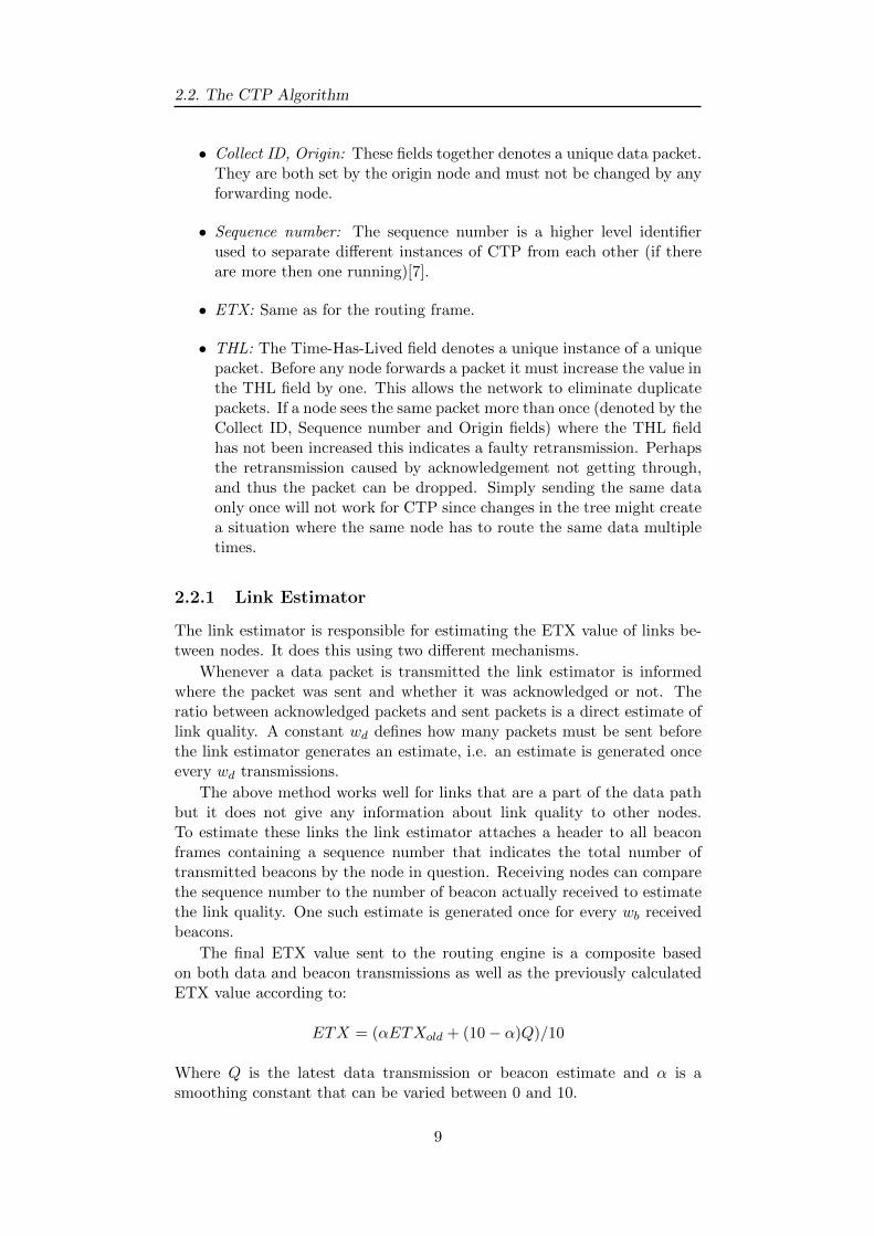
• Collect ID, Origin: These fields together denotes a unique data packet.They are both set by the origin node and must not be changed by anyforwarding node.

• Sequence number: The sequence number is a higher level identifierused to separate different instances of CTP from each other (if thereare more then one running)[7].

• ETX: Same as for the routing frame.

• THL: The Time-Has-Lived field denotes a unique instance of a uniquepacket. Before any node forwards a packet it must increase the value inthe THL field by one. This allows the network to eliminate duplicatepackets. If a node sees the same packet more than once (denoted by theCollect ID, Sequence number and Origin fields) where the THL fieldhas not been increased this indicates a faulty retransmission. Perhapsthe retransmission caused by acknowledgement not getting through,and thus the packet can be dropped. Simply sending the same dataonly once will not work for CTP since changes in the tree might createa situation where the same node has to route the same data multipletimes.

2.2.1 Link Estimator

The link estimator is responsible for estimating the ETX value of links be-tween nodes. It does this using two different mechanisms.

Whenever a data packet is transmitted the link estimator is informedwhere the packet was sent and whether it was acknowledged or not. Theratio between acknowledged packets and sent packets is a direct estimate oflink quality. A constant wd defines how many packets must be sent beforethe link estimator generates an estimate, i.e. an estimate is generated onceevery wd transmissions.

The above method works well for links that are a part of the data pathbut it does not give any information about link quality to other nodes.To estimate these links the link estimator attaches a header to all beaconframes containing a sequence number that indicates the total number oftransmitted beacons by the node in question. Receiving nodes can comparethe sequence number to the number of beacon actually received to estimatethe link quality. One such estimate is generated once for every wb receivedbeacons.

The final ETX value sent to the routing engine is a composite basedon both data and beacon transmissions as well as the previously calculatedETX value according to:

ETX = (αETXold + (10− α)Q)/10

Where Q is the latest data transmission or beacon estimate and α is asmoothing constant that can be varied between 0 and 10.

9


2.2.2 Routing Engine

The routing engine has two main responsibilities. It is responsible for choos-ing a parent, and therefore indirectly for constructing the tree, and for send-ing out beacons to inform other nodes of its status as described in Section 2.2.

The choice of parent is done by storing all neighbour’s ETX values in atable together with estimates of link ETXs generated by the link estimator,and picking the parent with the smallest total ETX. Also if network condi-tions change, the routing engine should switch to a new parent if the newone has an ETX substantially better then the old one. How much betterthe new ETX has to be to trigger a switch is defined by a preset thresholdvalue.

2.2.3 Forwarding Engine

The forwarding engine has several responsibilities[5], first and foremost fordeciding what to do with incoming packets (received or locally generated). Itis responsible for signalling the application layer receive function if the nodeis a root or forwarding the packet to the next hop if it is not. The forwardingengine also schedules packets for retransmissions a limited number of timesif acknowledgements are not received. The time between two transmissionsis random within a specified interval.

It is also responsible for maintaining the transmission queue and detect-ing and stopping duplicate transmission caused by acknowledgements notgetting through to children of the node. Finally it detects inconsistenciesin the tree by monitoring the ETX field of the CTP header in all incomingdata packets and informing the routing engine of any errors.

10

CHAPTER

3

COMPENSATING FOR LOSTPACKETS

The CTP algorithm described in the previous chapter is capable of findingthe best way to send information through a network. Sometimes howevereven the best way is not good enough and the CTP will struggle to deliverdata packets to the actuator in a timely fashion. Such delays and outagescombined with the fact that the CTP inevitably will drop some packets whenchanging routes if the connection to the old route was completely lost, callsfor a control strategy capable of handling various outages. In this thesisa Predictive Outage Compensator (POC)[2] implemented in the actuatoris suggested to solve this problem by filling in the information lost in thenetwork.

This chapter starts with an introduction to the terminology used andcontinues with the derivation of a closed loop system on state space form.The next Section introduces the concept of outage compensation and thetheory behind the optimal stochastically synthesized POC, also referred toas the Kalman based POC. Finally two alternative naive approaches thatwill be used for comparison are presented.

3.1 Introduction

As a first step towards the closed loop system the terminology for the process,controller and disturbance model is established. Consider the process P ondiscrete state space form

P{x+p = Apxp + Buu + Bdd

y = Cpxp + n(3.1)

where y is the desired output and u is the input given by the controller C

C{x+c = Acxc + Bce

u = Ccxc + Dce(3.2)

11

Compensating for Lost Packets

where e is the control error. The measurement noise n is considered to bea vector of white uncorrelated noise and the process noise d is given by D

D{x+d = Adxd + Bww

d = Cdxd + Dww(3.3)

where w is a vector of white uncorrelated noise.

3.2 The Closed Loop System

The goal in this Section is to derive the closed loop system with the referenceand noises as inputs and the control signal as output. The control error eis first considered to be the difference between some reference r and theprocess output y according to

e = r− y

Inserting u from (3.2) and d from (3.3) in (3.1) yields:

x+p = Apxp + BuCcxc + BuDcr−BuDcy + BdCdxd + BdDww

= (Ap −BuDcCp)xp + BuCcxc + BdCdxd + BuDcr + BdDww −BuDcn

Inserting y from (3.1) in (3.2) yields:

x+c = −BcCpxp + Acxc + Bcr−Bcn

Using the two equations above together with (3.3) the complete closed loopsystem on state space form evolves as:

x+p

x+c

x+d

=

Ap −BuDcCp BuCc BdCd

−BcCp Ac 00 0 Ad

︸︷︷︸

Acl

xpxcxd

︸︷︷︸

xcl

+

BuDc

Bc

0︸︷︷︸Br

BdDw −BuDc

0 −Bc

Bw 0︸︷︷︸N

︸︷︷︸

Bcl

rwn

︸︷︷︸

ucl

u =(−DcCp Cc 0

)︸︷︷︸Ccl

xpxcxd

+

Dc︸︷︷︸Dcl1

0 −Dc︸︷︷︸Dcl2

︸︷︷︸

Dcl

rwn

(3.4)

12

3.3. Outage Compensation

3.3 Outage Compensation

The goal of outage compensation is to have some intelligent method of es-timating a signal when no actual data is received from the network. Asmentioned before this thesis investigates the possibility of implementing thisintelligence in the actuator node.

3.3.1 Designing a Kalman Based POC

In this Section the closed loop system from Section 3.2 is used to derive astochastically synthesized POC capable of estimating the control signal u.To start, the system in (3.4) can be rewritten as

x+cl = Aclxcl + Brr + N

(wn

)︸︷︷︸v1

u = Cclxcl + Dcl1r + Dcl2

(wn

)︸︷︷︸

v2

(3.5)

Given this system the optimal estimator of the states xcl is the Kalman filter

POC{x+cl = Aclxcl + Brr + K(u− u)

u = Cclxcl + Dcl1 r(3.6)

where xcl and u are the estimates of the closed loop states and controlsignal respectively. The estimator uses r as the reference and r is updatedaccording to

r =

{r If no outage

r− During outage

The optimal feedback gain K is calculated through solving the discretetime Riccati equation[8, p. 158]

P = APAT + NR1NT − (APCT + NR12)(CPCT + R2)−1(APCT + NR12)T

K = (APCT + NR12)(CPCT + R2)−1

(3.7)

where A = Acl, C = Ccl and N all come from (3.5). The noise covariancematrices are given by

13


R1 = E[v1vT1 ] =

E[w1w1] · · · E[w1wi] E[w1n1] · · · E[w1nj ]...

. . ....

.... . .

...E[wiw1] · · · E[wiwi] E[win1] · · · E[winj ]E[n1w1] · · · E[n1wi] E[n1n1] · · · E[n1nj ]

.... . .

......

. . ....

E[njw1] · · · E[njwi] E[njn1] · · · E[njnj ]

=

V ar(w1) 0 0 0 0 0

0. . . 0 0 0 0

0 0 V ar(wn) 0 0 00 0 0 V ar(n1) 0 0

0 0 0 0. . . 0

0 0 0 0 0 V ar(nm)

R2 = E[v2v

T2 ] = E[(Dv1)(Dv1)

T ] = DE[v1vT1 ]D

T = DR1DT

R12 = E[v1vT2 ] = E[v1(Dv1)

T ] = E[v1vT1 ]D

T = R1DT

(3.8)

where D = Dcl2 and assuming that w is a vector of i uncorrelated noisesand n is a vector of j uncorrelated noises.

The POC in (3.6) is implemented according to the block diagram inFigure 3.1. When there is no outage the estimator error ε = u − u is usedto update the estimator states according to (3.6). When outage occurs ε isassumed to be zero and the states are updated and control signal estimatedaccording to

x+cl = Aclxcl + Brr

u = Cclxcl + Dcl1 r

P

D

C

POC

r

nw

r

+

+

+

y

e

u

u|u

u

ε

dPOC on

POC off

−

−

Figure 3.1: Block diagram of the Predictive Outage Compensator implementedto estimate the control signal u.

14

3.3. Outage Compensation

State reduction

For complex processes run by advanced controllers and with intricate dis-turbance models it is most likely that the closed loop system in (3.5) willbecome even more complicated. Since the number of states in xcl is thecombined sum of the number of states in xp, xc and xd it might be good toreduce the the system to a lower order. The goal of such a reduction is to, asaccurately as possible, describe the relation between input and output usinga smaller number of states. There are several methods for performing thereduction, for example singular perturbation, balanced truncation or Hankelapproximation. Using any of these methods on the final POC system (3.6),it can be rewritten as

x+rcl = Ar

clxrcl + Br

rr + Kr(u− ur)

ur = Crclx

rcl + Dr

cl1 r

where xrcl is the state vector with a reduced number of states. It is goodto keep in mind that any physical interpretation of the system states is lostafter doing the reduction even if the input/output relation remains similar.

3.3.2 Zero Compensator

A zero compensator is perhaps the most simple form of compensator. Im-plemented in the actuator a zero compensator would estimate the controlsignal according to

u =

{u If no outage

0 During outage

It could be argued that setting the control signal to zero when all feed-back is lost is a safe option. This is especially true if applied to a processthat require zero control signal to maintain stationarity i.e. a process thathas a pure integration as a part of its model. An example of such a processis a robot arm that moves when voltage is applied to a motor and sits stillwhen no voltage is applied. In this thesis the zero compensator will be usedas a benchmark for the stochastically synthesized POC from Section 3.3.1.

3.3.3 Hold Compensator

The hold compensator is arguably the most commonly used form of outagecompensator. It follows a do nothing approach where the actuator simplydoes not update the control signal if no new data is received.

u =

{u If no outage

u− During outage

It is easy to imagine that a hold compensator would be a good optionfor a system that spends most of its time in stationarity while systems with

15


many transients will suffer from the hold strategy. The hold compensatorwill provide a second benchmark for the stochastically synthesized POCfrom Section 3.3.1.

16

CHAPTER

4

IMPLEMENTATION

This Chapter describes the implementation of the CTP and the POC in asmall networked control system running the double tank process. The readeris first given necessary information about the hardware used in the networkand about the double tank process itself, including how its mathematicalmodel can be derived. Using the knowledge about the system the TinyOSimplementation of CTP is adapted and the POC parameters are calculated.The implementation of the POC into TinyOS is also described.

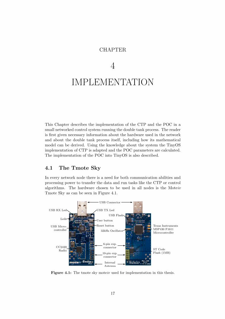
4.1 The Tmote Sky

In every network node there is a need for both communication abilities andprocessing power to transfer the data and run tasks like the CTP or controlalgorithms. The hardware chosen to be used in all nodes is the MoteivTmote Sky as can be seen in Figure 4.1.

USB Connector

USB TX Led

USB Flash

User button

Reset button

32kHz Oscillator

6-pin exp.connector

InternalAntenna

10-pin exp.connector

Texas InstrumentsMSP430 F1611Microcontroller

ST CodeFlash (1MB)

USB RX Led

Leds

USB Micro-controller

CC2420Radio

Figure 4.1: The tmote sky moteiv used for implementation in this thesis.

17

Implementation

The Tmote Sky has all the equipment needed to work in a wireless controlnetwork application. Its key features include[9]:

• A 250kbps, 2.4GHz, IEEE 802.15.4 Chipcon Wireless Transceiver tocommunicate with other 802.15.4 compliant devises.

• 8MHz Texas Instruments MSP430 micro controller for performing cal-culations.

• Integrated ADC and DAC for easy connection to any analogue sensorsand actuators.

• Integrated on-board antenna with 50m/125m range (indoors/outdoors).

• Ultra low current consumption that enables the device to run on bat-teries for extended periods of time.

• Programming and data collection to desktop computers via USB.

• 16-pin expansion support for connection to external devices.

• TinyOS support.

• User programmable button and three leds.

For more information on the Tmote Sky, please refer to the data sheet[9].

4.2 The Double Tank Process

The CTP and POC algorithms presented in previous Chapters can be im-plemented on any process that can be modelled reasonably well by a linearand time-invariant (LTI) system. In this thesis the Quanser double-tankprocess will be used to evaluate the performance of the implementation.

The Quanser double tank process in Figure 4.2 has four major compo-nents. Two tanks, one upper and one lower, a basin and a pump poweredby an electric motor. Furthermore there are two pressure sensors measuringthe water level in both the upper and the lover tank and a tap that allowsfor manual draining of water from the upper tank.

During operation the pump draws water from the basin and dumps itin the upper tank. Water then flows from the upper tank through a nozzleinto the lover tank and then back to the basin through another nozzle.

In Figure 4.2b A indicates the cross sectional area of both tanks whilea1 and a2 are outlet hole areas for the upper and lover tanks respectively.The tank levels are x1 and x2 and they are also the system’s states as willbe demonstrated in Section 4.2.1. The pump voltage u is the input to thesystem.

Figure 4.2a shows the real double-tank system together with the uni-versal power module (UPM). On top of the UPM sits the connector panelfor the sensor and actuator motes as well as a first order low-pass filter forremoving high frequency disturbances from the sensor data. The crossoverfrequency of the filter is chosen to half the sampling frequency according tothe Nyquist criterion.

18

4.2. The Double Tank Process

(a) The double tank process to-gether with the universal powermodule.

x1

x2

A

A

a1

a2

Upper

Tan

k

Low

erTan

k

+u

Tap

(b) Diagram of the double tankprocess.

Figure 4.2: The double-tank process

4.2.1 Modelling

To have a good mathematical model of the process is important when doingany kind of model based control. For this implementation a good modelwill help create an estimator that accurately estimates the control signal incase of communication failure. The model will also enable quick and easyPID-regulator design possibilities in Matlab.

For deriving the model a gray box approach is used where knowledge ofthe system is combined with data from experiments to form a model. It issuggested that the upper tank can be modelled as a first order system withthe control signal u as input according to

X1(s) =k

1 + τsU(s) (4.1)

where k is the gain of the process and τ is the time constant. Furthermorethat the lower tank can be modelled as

X2(s) =γ

1 + γτsX1(s) (4.2)

where the input is the water level in the upper tank and γ is a constantrelating the level in the upper tank to the level in the lower tank at steadystate.

The constants k, τ and γ from the two sub systems above were derivedfrom a step experiment on the actual double tank process. First a constantvoltage of u0 = 5.9 V was applied to the motor and the process was given

19

Implementation

time to stabilize. At time ts = 50 s a step was made in the voltage tous = 7.3 V. The recorded data is shown in Figure 4.3a.

0 50 100 150 20010

12

14

16

Time [s]

Waterlevel[cm]

x1x2

(a) Real process.

0 50 100 150 200

26

28

30

32

Time [s]

Waterlevel[cm]

x1x2

(b) Derived model.

Figure 4.3: Step responses of the double tank system and its model.

The gain k of sub system (4.1) is found as the ratio between the changein water level for the upper tank and the change in voltage.

k =x1s − x10us − u0

=0.169− 0.107

7.3− 5.9= 0.0443 m/V

The time constant τ is defined as the time it takes for the water level in theupper tank to reach 1− e−1 of the total step size. From the plot in Matlabit can be read that

τ = 18.1444 s

Finally γ can be calculated from the water levels at t = 0 s as previouslydescribed.

γ =x20x10

=0.103

0.107= 0.9626

The two systems (4.1) and (4.2) evolve as

X1(s) =0.0443

1 + 18.1444sU(s)

X2(s) =0.9626

1 + 17.4661sX1(s)

The last step is to rewrite the transfer functions into a state space repre-sentation of the double tank process. This is done by converting each of thesub systems into observable canonical form as in[10, p. 159]. The advantageof this method is that the states in the state space representation will corre-spond to the two tank levels which makes the notation more understandable.The complete process model on state space form with the lower tank waterlevel as output is

x =

(−0.05511 00.05511 −0.05725

)x +

(0.002441

0

)u

y =(0 1

)x

(4.3)

The model above was tested in Simulink with the same voltage step aspreviously applied to the real process. The simulated water levels for both

20

4.3. Implementation of a Small CTP Network

the upper and lower tanks are shown in Figure 4.3b. The water levels aremuch higher in the simulation compared to the experimental data. This isdue to the fact that the tank system is not linear and thus that the model willonly be valid for water levels close to x0 and xs. The time characteristics andstep size of the simulation is almost exactly the same as in the real systemand ratio between lower and upper tank is equal to γ. The conclusion isthat (4.3) is a good enough model to use when implementing the POC.

To create a more realistic simulation environment a set of non-linearequations for the double tank process was derived from Newtonian relationsand Bernoulli’s law.

x1 = −α1

√2gx1 + βu

x2 = α1

√2gx1 − α2

√2gx2

The constants α1, α2 and β can be estimated using the constants derived inthe experiment above.

τ =1

α1

√2x10g

, γ =α21

α22

, k = βτ

4.3 Implementation of a Small CTP Network

In TinyOS 2.0 an implementation of CTP is available in the tos/lib/netdirectory. It implements the CTP algorithm using a link estimator, a routingengine and a forwarding engine as described in Sections 2.2.1-2.2.3. Thereare many parameters in the implementation that can be varied to manipulatethe performance of the network. The choice of ideal parameters depends onmany different things, for example the size of the network, network load,delay tolerances and what types of network disturbances are common.

For the implementation of a small CTP network between the controllerand the actuator in the double tank control system the parameters seen inTable 4.1 were used. Experiments will show that these parameters workwell for the double tank process with 1 s sampling time in a laboratoryenvironment. Also from this point on a network will be considered to havea singular source (a sensor node) rather then multiple where other nodes inthe network simply pass information towards the root (the controller).

In a CTP network all nodes are allowed to choose any other node in rangeas their parent. This creates problems with experimental repeatability sinceit is extremely hard to foresee all radio conditions that will influence thenodes choice of parent. To minimize this problem the routing engine wasmodified to only allow a node to chose from a certain set of parents. Thismade it possible to create the semi static routing tree shown in Figure 4.4.

In the semi static tree the CTP is running its standard operations but anodes choice of parent is limited according to the arrows in the Figure. Onlynode R3 has a choice to send data down one of two available paths.

21

Implementation

Parameter Value Unit

Link Estimator:

α 7 -wd 5 packetswb 3 packets

Routing Engine:

Minimal beacon window length 128 msMaximal beacon window length 10 sParent switch threshold 5 -Parent refresh period 8192 ms

Forwarding Engine:

Maximum retransmissions 6 -Time to hold before retransmission 15-30 ms

Table 4.1: Table of tunable constants for a CTP network.

Controller(Source)

R3

R2 R1

R4 R5

Actuator(Root)

Routing net

Figure 4.4: The semi static route implementation of CTP.

4.4 The Kalman Based POC

This Section describes the synthesis of the Predictive Outage Compensatortheory from Section 3.3.1 with the double tank process model derived ear-lier in this Chapter. The goal is a POC on state space form as in (3.6)implemented in TinyOS.

To achieve this goal all the discrete state space functions described inSection 3.1 needs to be calculated. A first step is to chose a sampling fre-quency for the system. As a rule of thumb it is good to sample 20 timesfaster then the open loop systems crossover frequency. However the sam-pling frequency can be somewhat reduced if the control design is, as in thiscase, done with a method that takes the sampling frequency into account. Achoice of sampling frequency Ts = 1 s is therefore motivated by the crossoverfrequencies presented later in this Section.

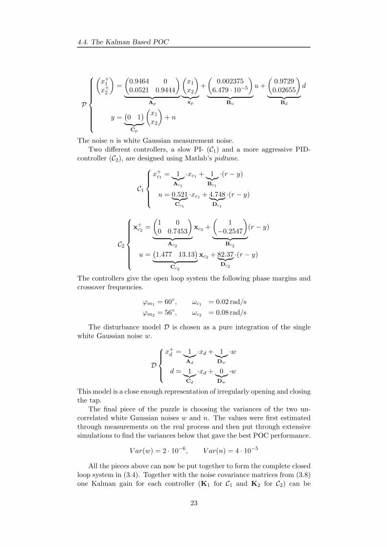
Looking at Figure 3.1 the process P is found by discretizing the model in(4.3) with the additional disturbance d added to the upper tank state. Thechoice of having the disturbance affect only the upper tank is motivated bythe design of the actual process, where the tap drains water from the uppertank only. For the discretization Matlab’s c2d function is used.

22

4.4. The Kalman Based POC

P

(x+1x+2

)=

(0.9464 00.0521 0.9444

)︸︷︷︸

Ap

(x1x2

)︸︷︷︸

xp

+

(0.002375

6.479 · 10−5

)︸︷︷︸

Bu

u+

(0.97290.02655

)︸︷︷︸

Bd

d

y =(0 1

)︸︷︷︸Cp

(x1x2

)+ n

The noise n is white Gaussian measurement noise.Two different controllers, a slow PI- (C1) and a more aggressive PID-

controller (C2), are designed using Matlab’s pidtune.

C1

x+c1 = 1︸︷︷︸

Ac1

·xc1 + 1︸︷︷︸Bc1

·(r − y)

u = 0.521︸︷︷︸Cc1

·xc1 + 4.748︸︷︷︸Dc1

·(r − y)

C2

x+c2 =

(1 00 0.7453

)︸︷︷︸

Ac2

xc2 +

(1

−0.2547

)︸︷︷︸

Bc2

(r − y)

u =(1.477 13.13

)︸︷︷︸Cc2

xc2 + 82.37︸︷︷︸Dc2

·(r − y)

The controllers give the open loop system the following phase margins andcrossover frequencies.

ϕm1 = 60◦, ωc1 = 0.02 rad/s

ϕm2 = 56◦, ωc2 = 0.08 rad/s

The disturbance model D is chosen as a pure integration of the singlewhite Gaussian noise w.

D

x+d = 1︸︷︷︸

Ad

·xd + 1︸︷︷︸Dw

·w

d = 1︸︷︷︸Cd

·xd + 0︸︷︷︸Dw

·w

This model is a close enough representation of irregularly opening and closingthe tap.

The final piece of the puzzle is choosing the variances of the two un-correlated white Gaussian noises w and n. The values were first estimatedthrough measurements on the real process and then put through extensivesimulations to find the variances below that gave the best POC performance.

V ar(w) = 2 · 10−6, V ar(n) = 4 · 10−5

All the pieces above can now be put together to form the complete closedloop system in (3.4). Together with the noise covariance matrices from (3.8)one Kalman gain for each controller (K1 for C1 and K2 for C2) can be

23

Implementation

calculated through solving the Riccati equation in (3.7). This was donenumerically using Matlab’s dare function.

K1 =

−0.2932−0.07510.2106−0.0394

, K2 =

−0.0147−0.00430.0121−0.0031−0.0023

4.4.1 Implementation in TinyOS

The program running in the actuator was designed to follow the structurein Figure 4.5. An important problem to solve when implementing the POCis how to decide when to use the estimate and when to wait for a packetwith the real control signal. The approach used in this thesis is an intuitivesolution based on the fact that the actuator knows approximately when toexpect a packet since the sampling time is well established.

Whenever a packet containing the control signal is received from thecontroller the actuator starts a countdown timer. The time to count downis set to the sampling time plus an extra delay. The extra delay is estab-lished based on the number of retransmissions and the time between eachretransmission. After this time the controller have surely dropped the packetand thus the POC should step in and estimate the control signal. For thisspecific application the delay time is set to 0.2Ts = 0.2 s and thus the timercounts down from 1.2 s. Before the program starts the estimation calcula-tions it resets the countdown timer but this time without the delay. This isnecessary to maintain the sampling frequency during long outages.

Start

Initialize

Newdata?

Start POC timer1.2 s

Update POC stateOutput u

POCtimer?

Start POC timer1 s

Update POC stateOutput u

yes

no

yes

no

Figure 4.5: Program structure of the POC implementation in the actuator.

24

CHAPTER

5

RESULTS

So far this thesis has described the theory behind the CTP algorithm andits implementation as a small network with routing restrictions. The idea ofoutage compensation has also been explained in theory and a stochasticallysynthesized POC for the double tank system has been designed. In this stepthe results of the above is presented both as simulation results and datafrom real experiments.

The first Section in this Chapter presents results from real experimentsperformed on the small CTP network described in Section 4.3. It continueswith a simulation study of the three different outage compensation methodspresented in Section 3.3 and ends with results from real experiments per-formed on the complete system with the CTP network active between thecontroller and actuator and a POC implemented in the actuator.

5.1 Evaluation of CTP Routing Performance

This Section aims to evaluate how the CTP network performs and identifyany weak spots that inevitably will have to be handled by the POC. Allexperiments were performed on the small CTP network illustrated in Fig-ure 4.4 with the nodes placed about 1 m apart in a laboratory environment.This means that the results presented here might not be representative ofhow the network would perform implemented in a real industry. To answerthis question the nodes would have to be placed further apart in the actualenvironment while handling more network traffic. Two types of experimentswere conducted each to answer the following:

• How will the multi-hop network between the controller and actuatoraffect the end-to-end delay between these nodes? What kind of packetloss is expected under close to ideal conditions in a laboratory.

• How does re-routing in the network affect the delay and number oflost packets?

25

Results

In the first experiment, dummy data was sent from the controller node tothe actuator node through the network while transmission times and num-ber of lost packets were monitored. The experiment ran for approximately40 min. Figure 5.1 shows the histogram of the end-to-end delays.

0 20 40 60 80 100 120 140 160 180 200 220 240 2600

200

400

600

Time [ms]

Packets

Figure 5.1: Histogram of end to end delay between controller and actuator in theCTP network.

The diagram shows a clear normal distribution of the delays around theaverage delay time 65.1 ms with very few stray packets. During this test nota single lost packet was recorded. The minimum delay time was recorded to46.8 ms and the maximum to 251.9 ms (a single stray packet).

Figure 5.2 shows the transportation of a single packet to help visualizewhat is going on in each node during the routing process. In this Figure they-axis represents the individual nodes and the x-axis represents the time.Different colors are used depending on in what node an event takes place.Black is for the controller, blue is for the actuator and red is for node R3.The lower path through R2 and R1 is represented by dark greed color andthe upper path through R4 and R5 by light green.

41.00 41.05 41.10 41.15 41.20

Cont.R3

R2

R1

R4

R5

ActuatorAction

Time [s]

Node

Figure 5.2: A single data packets route through the network.

The Figure illustrates the following. The controller starts by sending apacket indicated by a dot on the controller line in the controller color (black).The packet is received by R3, indicated by a red cross, and R3 acknowledgesthe packet. The acknowledgement is received at the controller and indicatedby an asterisk. R3 then tries to send the packet to R2 (the first red dot)but the transmission fails leading to retransmissions (the subsequent dots).A square (not present in Figure 5.2) would indicate that a packet has beenretransmitted the maximum number of times and therefore dropped. Thered triangle on the action line indicates a decision made by R3 to change itsparent and sent the packet toR4 instead. The rest of the transmission follows

26

5.1. Evaluation of CTP Routing Performance

the same structure. Note that the times on the x-axis is not 100 % accuratedue to delays and collisions in the serial communication between the motesand the computer recording the data. These Figures should therefore onlybe used to analyse what is happening in the network and not to measuretime intervals and such.

The next trial was designed to test the effects of re-routing. Just asbefore the nodes were set up according to Figure 4.4 sending dummy datafrom the controller to the actuator. For the experiment the following stepswere then taken.

1. Block connection between node R3 and its parent (R2 or R4) at timet = 40 s.

2. Re-open the connection at time t = 80 s.

3. Block connection one step further down the data path (between R2

and R1 or R4 and R5) at time t = 140 s.

4. Re-open the connection at time t = 180 s.

5. End experiment at time t = 220 s.

The connection was blocked by turning off the radio of the receiving nodein software. The test was repeated several times, half of the times accordingto the list above and half with step 1 and 3 in the opposite order. It wasdone this way to reduce the impact of ETX build-up.

Whenever the route has to change due to a complete communicationbreakdown as in this case (turning of the radio of the receiving node) thenetwork always drops one or more packets. Figure 5.3 shows the reroutingfor the two cases, blocking a node close to R3 and blocking a node far fromR3.This Figure illustrates the typical difference between blocking a node closeto, and far from the node that has to make the switch. Far fewer packetsare lost if the node blocked is close the the node switching parent. Thisobservation is supported by theory. When node R5 in Figure 5.3b is blockedR4 can no longer deliver its packets and thus increases its ETX. This ETXis then broadcasted with every beacon sent by R4 and sooner or later R3

will hear the beacon, discover that R2 is now a better parent and make theswitch. In the case as in Figure 5.3a when R2 is blocked, R3 discovers thisdirectly since none of its packets gets acknowledged. The information doesnot need to propagate through the network and the switch happens faster.

On average the network drops 1.75 packets when R2 or R4 is blockedand 4.25 packets when R1 or R5 goes down, but up to 8 dropped packets ina row has been observed during the experiments. This is one of the reasonswhy it is important to have an outage handling system in place.

27

Results

39 39.5 40 40.5 41

Cont.R3

R2

R1

R4

R5

ActuatorAction

Time [s]

Node

(a) R2 blocked.

139.5 140 140.5 141 141.5 142 142.5 143 143.5

Cont.R3

R2

R1

R4

R5

ActuatorAction

Time [s]

Node

(b) R5 blocked.

Figure 5.3: Figures showing several packets way through the network and thererouting process when a node is blocked.

28

5.2. Simulation of POC Performance

5.2 Simulation of POC Performance

Extensive simulation work has been done on the stochastically synthesizedPOC as well as on the hold and zero compensators. The goal has been tofind the best performing Kalman based POC and to compare that POC tothe less complicated compensation strategies.

To reduce the number of varying parameters in the simulations the fol-lowing static operating scenario was chosen:

• At all times. Measurement noise n with variance V ar(n) = 4 · 10−7 mis added to the process output. In the Figures below the noise isnot shown however it is a part of the feedback to the controller andcompensator.

• At t = 0 s. Water levels stable, r = x2 = 0.1 m. Simulation starts.

• At t = 100 s. Step in reference, r = 0.16 m.

• At t = ds = 230 s. A disturbance simulated as a constant drain of0.003 m/s from the upper tank starts. Note that this disturbance isnot the integrated white noise used for the design of the POC but amore realistic disturbance emulating opening of the tap.

• At t = de = 280 s. Constant drain from upper tank stops.

• At t = 500 s. Simulation ends.

This left the following parameters to be varied:

• Type of controller. One slow (C1) and one fast (C2) controller as de-scribed in Section 4.4.

• Outage start time. Varied between 0 s and 400 s in steps of 5 s.

• Outage duration. Varied between 0 s and 100 s in steps of 5 s.

• Type of outage compensation. Kalman based POC, hold compensatorand zero compensator.

To quantitatively evaluate the performance of the regulator and com-pensator together the integrated absolute error (IAE) was used.

IAE =

∫ ξ

0|e(t)| dt

With ξ = 500 s, the end time, the simulation was first run without outagesto get a baseline for the IAE for each controller.

C1 → IAE0 = 6.3080 m s C2 → IAE0 = 2.0068 m s

This baseline is in a way a measure of the pure control performance but itdoes not consider requirements on for example overshoot. Figure 5.4 showsthe simulated performance of both controllers. The Figure shows that C2 isfaster but gives a higher overshoot especially in the upper tank.

29

Results

0 100 200 300 400 500

12

14

16

18

20

Time [s]

Waterlevel[cm]

x1x2r

ds de

0 100 200 300 400 500

5

6

7

8

9

Time [s]

Pumpvoltag

e[V

]

uu

ds de

(a) Slow controller C1.

0 100 200 300 400 500

12

14

16

18

20

Time [s]

Water

level[cm]

x1x2r

ds de

0 100 200 300 400 500

5

6

7

8

9

Time [s]

Pumpvoltag

e[V

]

uu

ds de

(b) Aggressive controller C2.

Figure 5.4: Figures showing simulated performance of both controllers withoutoutages.

30


0 100 200 300 4000

50

100

0

1

2

Start time

Duration

IAE

n

(a) C1, Kalman POC.

0 100 200 300 4000

50

100

0

2

4

Start time

Duration

IAE

n

(b) C2, Kalman POC.

0 100 200 300 4000

50

100

0

1

2

Start time

Duration

IAE

n

(c) C1, hold compensator.

0 100 200 300 4000

50

100

0

5

Start time

Duration

IAE

n

(d) C2, hold compensator.

0 100 200 300 4000

50

100

0

5

Start time

Duration

IAE

n

(e) C1, zero compensator.

0 100 200 300 4000

50

100

0

10

20

Start time

Duration

IAE

n

(f) C2, zero compensator.

0 100 200 300 4000

50

100

−1

0

1

Start time

Duration

IAE

n

(g) C1, Kalman-hold comparison

0 100 200 300 4000

50

100

0

5

Start time

Duration

IAE

n

(h) C2, Kalman-hold comparison

Figure 5.5: Figures illustrating how the normalized IAE is affected by outageswith varying duration starting at different times.

31

Results

The real multi case simulation was then started, varying all the parame-ters listed above and returning data from 10126 unique cases. The 3D-plotsin Figure 5.5 visualize all that data. On the z-axis is the normalized IAE.

IAEn =IAE

IAE0

This normalized value can be interpreted as how much worse the controlperformance becomes due to the various outages. The x-axis shows thestart time of the outage and the y-axis its duration. Plots on the left handside of Figure 5.5 represent simulations done with the slow controller andthose on the right with the more aggressive one.

The first thing noticeable when studying the plots is that the zero com-pensator performs worse than both the hold and Kalman based compen-sators under every possible outage scenario. This result was expected know-ing that the double tank process is a system that requires a non zero inputto maintain a non zero water level. For this reason the zero compensatorwill not be considered further in this thesis.

The second observation is the three major peaks presented in Figures 5.5a-5.5d. These peaks correspond to large the changes in the system such asmaking a step in the reference, opening the tap and closing the tap. Finallyit is noted that there is an almost linear relation between outage durationand deterioration of control performance for a given outage start time.

By comparing the peaks of the plots corresponding to C1 to those cor-responding to C2 it is possible to draw the conclusion that outages causemore harm in a system with a fast controller. This conclusion can be refineda bit by comparing Figure 5.5c to Figure 5.5d. Given a static operationscenario as in this case, the system with the slow controller is more likelyto be in a transient when the outage occurs. This is bad, especially for thehold compensator, and results in the wider peaks seen in Figure 5.5c. Withan aggressive controller the system is more likely to be stationary, but ifthe outage occurs when it is not, the results become more severe, leading tohigher and thinner peaks.

One way to compare the two compensation methods, Kalman basedPOC and hold compensation, is to calculate the ratio between the sums ofall outages for the hold compensator and the Kalman based POC.∑

all outages

IAEholdn∑all outages

IAEkaln

=

{1.0118 for C11.0861 for C2

Using IAE as a measurement of control performance this indicates that thehold compensator performs 1.2 % worse with the slow controller and 8.6 %worse with the fast one. Another way to compare them is to study theFigures 5.5g and 5.5h which shows the differences in IAEn between the two.Positive values in the 3D-plots indicates that the Kalman POC performsbetter then the hold compensator for that particular outage case. The valuesof the plots are mostly positive.

32


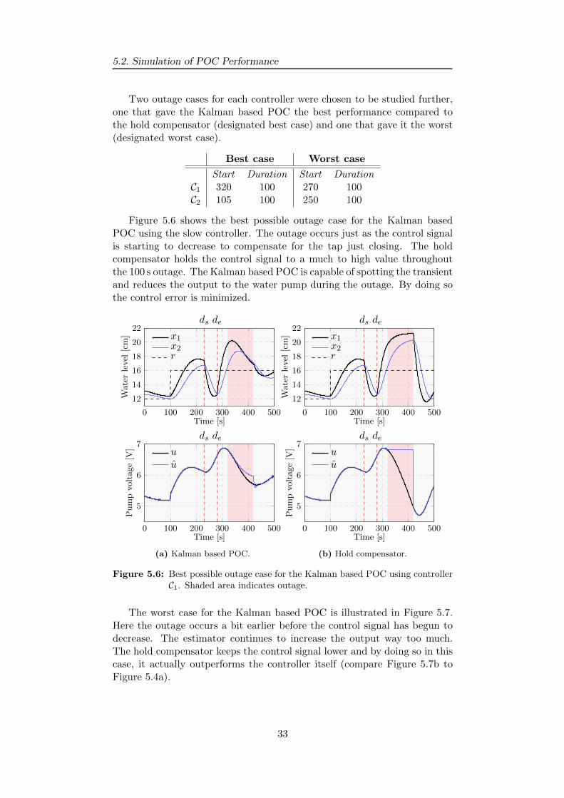
Two outage cases for each controller were chosen to be studied further,one that gave the Kalman based POC the best performance compared tothe hold compensator (designated best case) and one that gave it the worst(designated worst case).

Best case Worst case

Start Duration Start DurationC1 320 100 270 100C2 105 100 250 100

Figure 5.6 shows the best possible outage case for the Kalman basedPOC using the slow controller. The outage occurs just as the control signalis starting to decrease to compensate for the tap just closing. The holdcompensator holds the control signal to a much to high value throughoutthe 100 s outage. The Kalman based POC is capable of spotting the transientand reduces the output to the water pump during the outage. By doing sothe control error is minimized.

0 100 200 300 400 500

12

14

16

18

20

22

Time [s]

Waterlevel

[cm] x1

x2r

ds de

0 100 200 300 400 500

5

6

7

Time [s]

Pumpvoltage[V

] uu

ds de

(a) Kalman based POC.

0 100 200 300 400 500

12

14

16

18

20

22

Time [s]

Waterlevel

[cm] x1

x2r

ds de

0 100 200 300 400 500

5

6

7

Time [s]

Pumpvoltage[V

] uu

ds de

(b) Hold compensator.

Figure 5.6: Best possible outage case for the Kalman based POC using controllerC1. Shaded area indicates outage.

The worst case for the Kalman based POC is illustrated in Figure 5.7.Here the outage occurs a bit earlier before the control signal has begun todecrease. The estimator continues to increase the output way too much.The hold compensator keeps the control signal lower and by doing so in thiscase, it actually outperforms the controller itself (compare Figure 5.7b toFigure 5.4a).

33

Results

0 100 200 300 400 50010

15

20

25

Time [s]

Waterlevel

[cm] x1

x2r

ds de

0 100 200 300 400 5004

5

6

7

8

Time [s]

Pumpvoltage[V

] uu

ds de


0 100 200 300 400 50010

15

20

25

Time [s]

Waterlevel

[cm]

x1x2r

ds de

0 100 200 300 400 5004

5

6

7

8

Time [s]

Pumpvoltage[V

] uu

ds de


Figure 5.7: Worst possible outage case for the Kalman based POC using controllerC1. Shaded area indicates outage.

0 100 200 300 400 500

12

14

16

18

20

Time [s]

Waterlevel

[cm]

x1x2r

ds de

0 100 200 300 400 500

4

6

8

Time [s]

Pumpvoltage[V

] uu

ds de


0 100 200 300 400 5000

5

10

15

20

25

30

Time [s]

Waterlevel

[cm] x1

x2r

ds de

0 100 200 300 400 5000

2

4

6

8

Time [s]

Pumpvoltage[V

]

uu

ds de


Figure 5.8: Best possible outage case for the Kalman based POC using controllerC2. Shaded area indicates outage. Note that the y-axes are scaleddifferently.

34


With the faster controller things become a bit more sensitive. Figure 5.8shows the best case for the Kalman based POC where the outage occurs justafter the step. This means that the estimator can continue the transient andreduce the control signal, finally stabilizing at the level it believes is correct.The hold compensator holds the output at the high level present just afterthe step, causing the tanks to fill up fast. Figure 5.8 also shows one of thebiggest problem with actuator based compensation methods, integral wind-up of the controller output. Since the level x2 does not reach r during theoutage, the controller will continuously integrate the resulting error. Thismeans that when the outage finally ends, the real control signal u might beeven more wrong then the estimate u leading to big overshoots.

Lastly Figure 5.9 shows the worst case for the Kalman based POC com-pared to the hold compensator. This case is similar the one in Figure 5.7.The outage occurs before the tap is closed. The Kalman based POC has noknowledge of this change in the system and floods the tanks with too muchwater. The hold compensator gets lucky as the outage happens before thecontrol signal has reached its peak.

0 100 200 300 400 5007

12

17

22

Time [s]

Waterlevel

[cm] x1 x2

r

ds de

0 100 200 300 400 500

0

2

4

6

8

Time [s]

Pumpvoltage[V

]

uu

ds de


0 100 200 300 400 500

12

15

18

21

Time [s]

Waterlevel

[cm] x1 x2

r

ds de

0 100 200 300 400 5002

4

6

8

Time [s]

Pumpvoltage[V

]

uu

ds de


Figure 5.9: Worst possible outage case for the Kalman based POC using controllerC2. Shaded area indicates outage. Note that the y-axes are scaleddifferently.

35

Results

5.3 Implemented POC Experiments

This Section contains results from real experiments on the double tank sys-tem controlled via a wireless CTP network with outage compensation imple-mented as a part of the actuator. The results are from tests similar to thosesimulated, implementing the best and worst outage cases for the Kalmanbased POC compared to the hold compensator. To break the connectionbetween the controller and actuator for a duration of 100 s the networknode R3 was shut down. For all experiments the more aggressive controllerC2 was used.

0 100 200 300 400 500

121416182022

Time [s]

Water

level[cm]

x1x2r

ds de

0 100 200 300 400 500

6

7

8

9

10

Time [s]

Pumpvoltage

[V]

uu

ds de

Figure 5.10: Data from real experiment showing the static operating scenariowithout outage.

Figure 5.10 shows the water levels, control signal and control signal esti-mate while running the static operating scenario suggested in the previousChapter. The results are as expected and by comparing them to the sim-ulation in Figure 5.4 it becomes even more clear that the model used forsimulation fits well with the actual system.

An experiment with a 100 s outage starting at t = 105 s was then run.Figure 5.11 shows this experiment and the results compare well to previoussimulations. If anything it can be said that the Kalman based POC performseven better in this real experiment, stabilizing x2 closer to r before theoutage ends leading to less integral wind-up.

As a final result the experiment was run with worst possible outage casefor the Kalman based POC compared to the hold compensator. Figure 5.12shows results that once again compare well to the simulated counterpart,allowing the same conclusions to be drawn.

36

5.3. Implemented POC Experiments

0 100 200 300 400 500

12

14

16

18

20

22

Time [s]

Waterlevel

[cm]

x1x2r

ds de

0 100 200 300 400 500

6

7

8

9

10

Time [s]

Pumpvoltage[V

] uu

ds de


0 100 200 300 400 5000

5

10

15

20

25

30

Time [s]

Waterlevel

[cm]

x1x2r

ds de

0 100 200 300 400 5000

2

4

6

8

10

Time [s]

Pumpvoltage[V

]uu

ds de


Figure 5.11: Data from real experiment with outage best suited for the KalmanPOC. Shaded area indicates outage. Note that the y-axes are scaleddifferently.

0 100 200 300 400 500

5

10

15

20

25

Time [s]

Waterlevel

[cm] x1 x2

r

ds de

0 100 200 300 400 500-3

0

3

6

9

Time [s]

Pumpvoltage[V

]

uu

ds de


0 100 200 300 400 50010

15

20

25

Time [s]

Waterlevel

[cm] x1

x2r

ds de

0 100 200 300 400 5002

4

6

8

10

Time [s]

Pumpvoltage[V

]

uu

ds de


Figure 5.12: Data from real experiment with outage best suited for the hold com-pensator. Shaded area indicates outage. Note that the y-axes arescaled differently.

37

CHAPTER

6

CONCLUSIONS

The goal of this thesis was to construct a simplified wireless control systemand then implement measures to overcome some of the drawbacks of wirelesscontrol. We have therefore investigated the Collection Tree Protocol routingalgorithm and the concept of outage compensation using a stochasticallysynthesized Predictive Outage Compensator.

Through the implementation of a CTP network we are able to avoidlengthy outages as long as there is at least one possible route from thecontroller to the actuator. In theory we have explained how this algorithmworks and in the implementation we have adapted it to suit the doubletank process in a laboratory environment. Through experiments we havethen tried to highlight the strong points of CTP such as its flexibility andconsistently low delay, despite using multi-hop. Tests have also illustratedweaknesses such as dropped packets during route changes, especially if thebreak occurs far from the decision making node.

Because of these network flaws it was necessary to develop a controlmethod that would keep the performance of the control system even if severaldata packets in a row were lost in the network. The POC suggested in thisthesis is based on a Kalman filter and therefore depend highly on a goodmodel of the closed loop system. We have shown through simulations andreal life experiments that the double tank system can highly benefit fromthe addition of a more advanced compensation method implemented in theactuator node. For the comparison we have used the two naive approaches,hold compensation and zero compensation. The Kalman based POC haveclearly shown better results.

6.1 Future Work

This thesis have answered several important questions but many remain andnew ones have been discovered. Interesting areas that we feel require morework are:

39

Conclusions

• Utilizing the advantages of CTPs mesh type architecture.The CTP network have, during our experiments, been restricted toa semi-static route where only one node has a choice of parent. Itwas done this way to enhance the repeatability of the experiments. Itis likely that the algorithm will perform better if not restricted andexperiments on big multi-hop mesh type CTP networks are thereforeof great interest.

• Experiments in a factory environment.The ultimate goal of this work is to develop a wireless network capableof controlling processes in a factory environment. To achieve this muchwork still needs to be done in the actual environment. For examplerunning experiments on a network under heavy load and with manyradio disturbances.

• Anti wind-up techniques.The weakest point of these actuator based compensators is their abilityto cause the controllers integral term to grow. Standard anti wind-uptechniques are hard to implement since the controller is not awareof the outage and thus this needs to be investigated further. Notethat a POC placed in the controller will not suffer from these wind-upeffects[3].

• Implementation of multiple POCs.The strength of having compensation in the actuator compared to thecontroller is that the actuator POC can handle outages no matterwhere in the control system they occur. On the other hand it suffersfrom the integral wind-up described above. It would be interesting toinvestigate how the system is affected if two POCs are implemented,both in the controller according to [3] and in the actuator.

40

BIBLIOGRAPHY

[1] Wikipedia article, Wireless.http://en.wikipedia.org/wiki/Wireless

Accessed 7 May 2012

[2] Erik Henriksson, Compensating for Unreliable Communication Links inNetworked Control Systems.Licentiate Thesis, 2009

[3] Ivar Cornell, Implementation of a Collection Tree Routing Protocol anda Predictive Outage Compensator.Master Thesis, 2012

[4] Wikipedia article, OSI model.http://en.wikipedia.org/wiki/OSI_model

Accessed 12 June 2012

[5] TinyOS TEP 123, The Collection Tree Protocol (CTP) v. 1.8.http://www.tinyos.net/tinyos-2.x/doc/html/tep123.html

Accessed 7 May 2012

[6] TinyOS TEP 119, Collection.http://www.tinyos.net/tinyos-2.x/doc/html/tep119.html

Accessed 16 May 2012

[7] Ugo Colesanti et. al, A Performance Evaluation Of The CollectionTree Protocol Based On Its Implementation For The Castalia WirelessSensor Networks Simulator.http://e-collection.library.ethz.ch/eserv/eth:5087/

eth-5087-01.pdf


[8] Torkel Glad, Lennart Ljung, Reglerteori. Flervariabla och olinjarametoder.Edition 2:5, 2009

[9] Moteiv, Tmote Sky Data Sheet.http://www.eecs.harvard.edu/~konrad/projects/shimmer/

references/tmote-sky-datasheet.pdf


[10] Torkel Glad, Lennart Ljung, Reglerteknik. Grundlaggande teori.Edition 4:3, 2007

41

network routing and unreliable communication link compensation555779/fulltext01.pdf · network...

Documents