network structure - دانشگاه آزاد اسلامی...

701

Available online at http://ijdea.srbiau.ac.ir

Int. J. Data Envelopment Analysis (ISSN 2345-458X) Vol. 1, No. 2, Year 2013 Article ID IJDEA-00126, 12 pages

Research Article

Non radial model of dynamic DEA with the parallel

network structure

S.Keikha-Javana, M.Rostamy-Malkhalifehb*

(a) Department of Mathematics, Zahedan Branch, Islamic Azad University, Zahedan, Iran.

(b) Department of Mathematics, Science and Research Branch, Islamic Azad University, Tehran,

Iran.

Abstract

In this article, Non radial method of dynamic DEA with the parallel network structure is presented

and is used for calculation of relative efficiency measures when inputs and outputs do not change

equally. In this model, DMU divisions under evaluation have been put together in parallel. But its

dynamic structure is assumed in series. Since in real applications there are undesirable inputs and

outputs in the proposed model, the assumption of the existence of the intermediate products have been

considered. After obtaining period–divisional efficiencies, by considering its weighted arithmetic

mean, models are presented for the evaluation of period, divisional and overall efficiency for decision

making unit

Keywords: dynamic data envelopment analysis – parallel network – overall efficiency – links and

variable carry-overs.

1 Introduction

Data envelopment analysis is a Non parametric method for measuring relative efficiency of decision

making units based on multiple inputs and outputs that was invented by Fare and universalized by

Charnes et al [2]. One of the drawbacks of this model is the omission of the internal structure of the

DMUs. For example, many companies and organizations are comprised of several divisions each one

of these division which specific inputs & outputs are linked together and other divisions as well. Also,

in real life the activities of such organizations are connected together in several different consecutive.

So, for the assessment of the performance of these organizations and companies a model is needed to

assess both the period efficiencies and divisional efficiencies and, eventually, the efficiency of overall

system.

For the first time in2000, Fare and Grosskopf [5] presented an article under the title of "Network data

envelopment analysis" in which the importance of network DEA was emphasized. After that, multiple

* Corresponding author, email:[email protected]

International Journal of Data Envelopment Analysis Science and Research Branch (IAU)

S.Keikha-Javan, et al /IJDEA Vol. 1, No. 2 (2013) 107-118 108

models of DEA with network structure were presented (for further studies one can refer to Costelli et

al [1] and Chen [3], Cook et al [4] and Lin et al [7]). Also Tone et al [8], developed network DEA

according to the SBM model. In this model links and carry-overs between divisions have specific

groupings (good link, fixed link). In addition to the structure of desired DMU division, they paid

attention to the connections between which this shows the development of network DEA model

towards internal structure of the assessed DMUs with the variable links. Ton et al [9], proposed a

combinatory model of two models of developed network DEA [8] and dynamic DEA for SBM model

[10]. This combinatory model not only enables us in the assessment of overall efficiencies of desired

DMU but also is a good guide for further analysis of the period efficiency and divisional efficiency of

DMUs.

In this paper the Non radial method of dynamic DEA with parallel network structure has been

presented with the assumption of the existence of various links & connections in the structure of the

network and dynamic model. Obtaining overall efficiencies, period efficiencies, divisional efficiencies

and period-divisional efficiencies in each period of time and in each part of DMUs’ decision making

sub-units con be assumed as one of the merits of this method considering the volatile links &

connections.

2 Dynamic DEA with parallel network structure

In dynamic DEA with parallel network structure we deal with decision making units n (DMUj,

j=1,…, n). Each DMU is divided to q divisions (p=1,…, q) which are placed parallel together.

Therefore overall system inputs are divided among all divisions and overall outputs results from the

output of all divisions. In this paper their efficiencies and the desired DMU efficiencies in T time

period (t=1,…,T) is examined.

The dynamic structure model consists of internal connections that transport intermediate products of t

period to t+1 period. In the first period, we don’t have any connection from previous period besides,

in the last period of T, we didn't consider any connection for the next period. We grouped these

connections into two groups of desirable and undesirable. Desirable carry-overs are treated as outputs

(transitional profit, net earned surplus) which we call them as “good” and undesirable carry-overs are

treated as inputs (loss carried forward, bad debt, dead stock) which are named “bad” accordingly. So

if we consider the number of all dynamic connections in this model as “h”, we will have:

(n-good) + (n-bad) =h

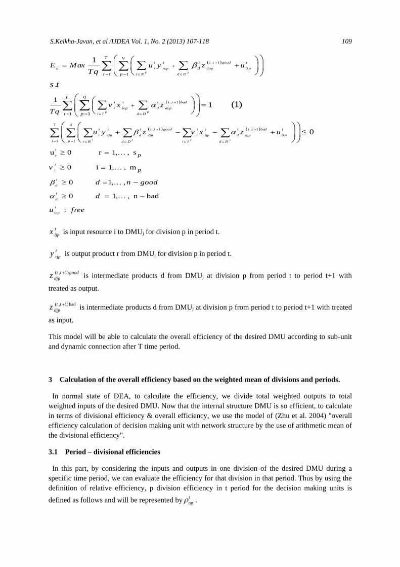
Non radial model dynamic DEA with parallel network can be expressed as follows:


. 1

0

, 1

T

, 1

t 1 1

1 1

1 1

1

1

1

.

(1)

p p

p p

p p

t t t t good t

o r rop dop p

r R d D

t t t t t bad

i iop d dop

i I d D

q

t t t t t good

r rjp d djp

p r R d D i

qT

t

d

t p

T

t

q

p

E Max u y z u

v x zTq

u y z

Tq

s t

, 1

0

t

r

0

u 0 r 1 , , s

0 i 1 , , m

0 1 , ,

0 1 , , n bad

:

0 p p

t t t t t bad t

i ijp d djp p

I d D

t

i

t

d

t

d

t

p

p

p

v x z u

v

d n good

d

u free

t

ijpx is input resource i to DMUj for division p in period t.

t

rjpy is output product r from DMUj for division p in period t.

( , 1)t t good

djpz

is intermediate products d from DMUj at division p from period t to period t+1 with

treated as output.

( , 1)badt t

djpz

is intermediate products d from DMUj at division p from period t to period t+1 with treated

as input.

This model will be able to calculate the overall efficiency of the desired DMU according to sub-unit

and dynamic connection after T time period.

3 Calculation of the overall efficiency based on the weighted mean of divisions and periods.

In normal state of DEA, to calculate the efficiency, we divide total weighted outputs to total

weighted inputs of the desired DMU. Now that the internal structure DMU is so efficient, to calculate

in terms of divisional efficiency & overall efficiency, we use the model of (Zhu et al. 2004) "overall

efficiency calculation of decision making unit with network structure by the use of arithmetic mean of

the divisional efficiency".

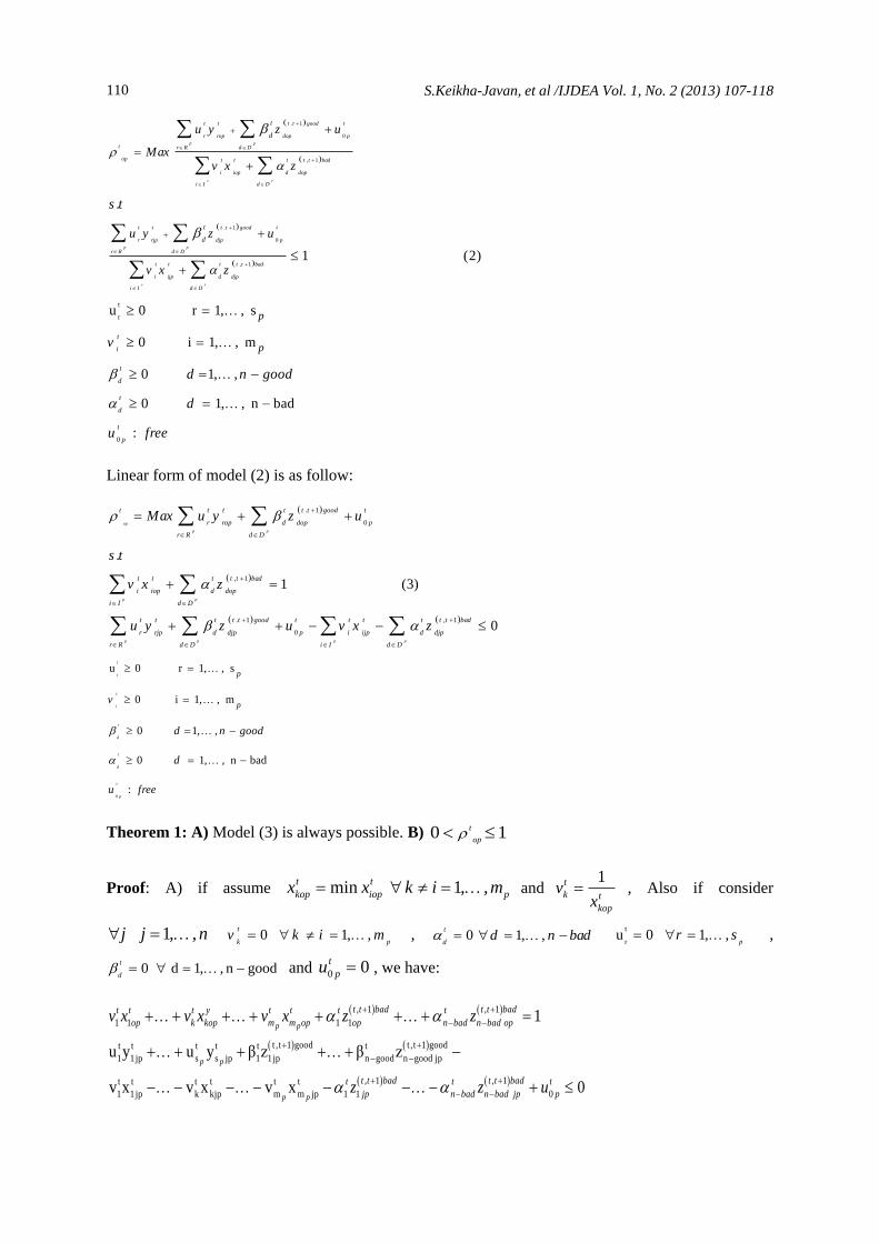
3.1 Period – divisional efficiencies

In this part, by considering the inputs and outputs in one division of the desired DMU during a

specific time period, we can evaluate the efficiency for that division in that period. Thus by using the

definition of relative efficiency, p division efficiency in t period for the decision making units is

defined as follows and will be represented byt

op .


. 1

0

, 1

. 1

0

, 1

.

1

p p

p p

p p

p p

t t t t good t

r rop dop p

t r R d D

op t t t t t bad

i iop d dop

i I d D

t t t t good t

r rjp djp p

r R d D

t t t t t bad

i ijp d djp

i I d D

t

d

t

d

u y z u

Maxv x z

u y z u

v x z

s t

t

r

0

(2)

u 0 r 1 , , s

0 i 1 , , m

0 1 , ,

0 1 , , n bad

:

t

i

t

d

t

d

t

p

p

pv

d n good

d

u free

Linear form of model (2) is as follow:

r

. 1

0

, 1

. 1 , 1

0

u

1 (3)

0

.

op

p p

p p

p p p p

t t t t t t good t

r rop d dop p

r R d D

t t t t t bad

i iop d dop

i I d D

t t t t t good t t t t t t bad

r rjp d djp p i ijp d djp

r R d D i I d D

Max

s

u y z u

v x z

u y z u v x z

t

t

0

0 r 1, , s

0 i 1, , m

0 1, ,

0 1, , n bad

:

t

i

t

d

t

d

t

p

p

pv

d n good

d

u free

Theorem 1: A) Model (3) is always possible. B) 0 1t

op

Proof: A) if assume min 1, ,t t

kop iop px x k i m and

1t

k t

kop

vx

, Also if consider

1, ,j j n 0 1, ,t

k pv k i m , 0 1, ,

t

dd n bad

t

ru 0 1, ,

pr s ,

0 d 1, , n good t

d and 0

0 t

pu , we have:

, 1 , 1

1 1 1 1

t ,t 1 good t ,t 1 goodt t t t t t

1 1jp s s jp 1 1jp n good n good jp

, 1t t t t t t

1 1jp k kjp m m jp 1 1

1

u y u y β z β z

v x v x v x

p p

p p

p p

t t bad t t badt t t y t t t t

op k kop m m op op n bad n bad op

t t badt

jp n

v x v x v x z z

z

, 1

00

t t badt t

bad n bad jp pz u


Model (3) is always possible.

B) Due to the previous possible solution and this fact that in each optimum solution at least one of

constraints multiplicand (Dual form) is as equality, we have:

n goods m n bad

t , t 1 good t , t 1 badt t t t t t

r r p d dop i iop d dop 0

r 1 d 1 i 1 d 1

u y β z v x α z 0t

o pu

n goods m n bad

t , t 1 good t , t 1 badt t t t t t

r r p d dop 0 i iop d dop

r 1 d 1 i 1 d 1

u y β z v x α z 1t

o pu

n goods

t , t 1 goodt t t

r rop d dop

r 1 d 1

u y β z 1

We know , 1

0t t good

djpz

,0

t

rjpy , 0

t

d ,

t

ru 0 . Then the sum of positive multi term is always

positive, so

s n good

t t t t , t 1 good

r rop d dop

r 1 d 1

u y β z 0

. We claim

s n good

t t t t , t 1 good

r rop d dop

r 1 d 1

u y β z 0

because if we suppose

contradiction

n goods

t t t t , t 1 good

r rop d dop

r 1 d 1

u y β z 0

then we will have:

n goods

t t t t , t 1 good

r rop d dop

R 1 d 1

u y β z

. This isn’t

compatible with positive total. 0 1t

op .

Definition 1: if* 1t

op , DMUo is called period-divisional efficient.

By noticing model (2) the period and division efficiency can be defined as convex linear combination.

3.2 Period efficiency

Period efficiency is actually the calculation of overall performance of the desired DMU divisions

that can only be evaluated in a specific time period. For this reason it is called period efficiency (the

single – period). Calculation of this efficiency is actually the calculation of the desired DMU

considering the efficiency of all their divisions. We display it byto . This efficiency can be evaluated

by the weighted mean of period – divisional efficiency (t

op ). Which is defined as follows:

1

4 q

t p to op

p

w

Notice that p

w weights shows the share of p division in the efficiency of the

desired period for the unit under evaluation and is

, 1

, 1

1

t t t t t bad

i iop d dop

p pi I d D

p p

q

t t t t t bad

i iop d dop

i I d Dp

p

v x z

w

v x z

. Due to this

definitionp

w ,1

1q

p

p

w

. Based on equation (4) we are period efficiency model as follows:


, 1

0

1

, 1

1

, 1

0

1

, 1

1

1 t, p, j

. :

p p

t

o

p p

p p

p p

qt t goodt t t t

r rop d dop pr R d Dp

qt t badt t t

i iop d dopi I d Dp

qt t goodt t t t

r rjp d djp pr R d Dp

t t badt t t

i ijp d djpi I

q

pd D

u y z u

v x z

s t

u y z u

v x

M x

z

a

t

r

0

u 0 r 1 , , s

0 i 1 , , m

0 1 , ,

0 1 , , n bad

:

5

t

i

t

d

t

d

t

p

p

pv

d n good

d

u free

Model (6) is linear model of from (5).

1

, 1

, 1

0

1

, 1 , 1

0

1

0 t, p, j

. :

11

1

p p

t

p po

q

p

p p p p

t t t t t bad

i iop d dopi I d D

q

t t goodt t t t

r rop d dop pr R d Dp

q

t t good t t badt t t t t t t

r rjp d djp p i ijp d djpr R d D i I d Dp

v x z

u y z u

s t

q

u y z u v x

Maxq

z

t

r

0

u 0 r 1, , s

0 i 1, , m

0 1, ,

0 1, , n bad

:

6

t

i

t

d

t

d

t

p

p

pv

d n good

d

u free

Theorem 2: A) Model (6) is always possible. B) 0 1t

o

Proof: is similarly to theorem 1 proving.

Definition2: if* t

1o , DMUo is called period efficient.

Corollary 1: *

1t

o if and only if

*1

t

op at least in one of the divisions.

3.3 Divisional efficiency

One of the benefits of calculating divisional efficiency is that the overall efficiency or inefficiency

could be assumed.


Also, if we want to calculate the performance of each one of desired DMU units in a long-time period,

we need to calculate divisional efficiency. Calculation this performance is in fact accounted efficiency

for each division in a long- time. We show divisional efficiency by op

and we define as the weighted

mean of period-divisional efficiency: 1

7

T

t t

op op

t

w

,t

w weight show the share t period in the

performance of the desired division for decision making unit and is

( , 1)

( , 1)

1

p p

p p

t t t t t

i iop d dop

t i I d D

T

t t t t t

i iop d dop

t i I d D

v x z

w

v x z

. Due to

the definition t

w we resulted1

1

T

t

t

w

.

By considering relation (7), divisional efficiency is defined like following:

, 1

0

1

, 1

1

, 1

0

1

, 1

1

1 t, p, j

. :

p p

p p

p p

p p

Tt t goodt t t t

r rop d dop pr R d Dt

op Tt t badt t t

i iop d dopi I d Dt

Tt t goodt t t t

r rjp d djp pr R d Dt

t t badt t t

i ijp d dj

T

t

pi I d D

Ma

u y z u

v x z

s t

u y z u

v x

x

z

t

r

0

u 0 r 1, , s

0 i 1, , m

0 1, ,

0 1, , n bad

:

8

t

i

t

d

t

d

t

p

p

pv

d n good

d

u free

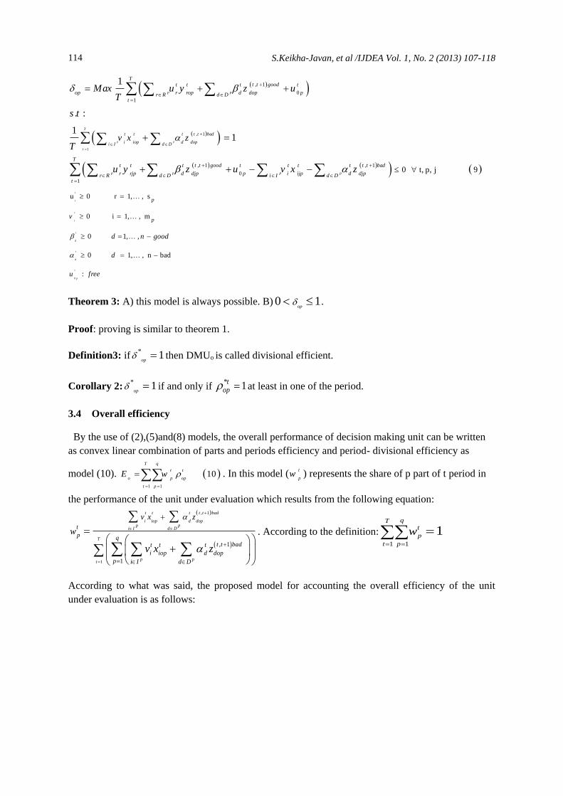
Model (8) can be changed in to linear model (9).


1

, 1

, 1

0

1

, 1 , 1

0

1

0 t, p, j

. :

11

1

p p

p p

T

t

p p p p

t t t t t bad

i iop d dopi I d D

Tt t goodt t t t

op r rop d dop pr R d Dt

Tt t good t t badt t t t t t t

r rjp d djp p i ijp d djpr R d D i I d Dt

v x z

u y z u

s t

T

u y

MaxT

z u v x z

t

r

0

u 0 r 1, , s

0 i 1, , m

0 1, ,

0 1, , n bad

:

9

t

i

t

d

t

d

t

p

p

pv

d n good

d

u free

Theorem 3: A) this model is always possible. B) 0 1op .

Proof: proving is similar to theorem 1.

Definition3: if*

1op

then DMUo is called divisional efficient.

Corollary 2:*

1op

if and only if *

1t

op at least in one of the period.

3.4 Overall efficiency

By the use of (2),(5)and(8) models, the overall performance of decision making unit can be written

as convex linear combination of parts and periods efficiency and period- divisional efficiency as

model (10). 1 1

10

qT

t t

o p op

t p

E w

. In this model (t

pw ) represents the share of p part of t period in

the performance of the unit under evaluation which results from the following equation:

, 1

1

, 1

1

t t t t t bad

i iop d dopp p

i I d

pt

T

D

p

t

p qt t badt t t

i iop d dop

p i I d D

v x z

w

v x z

. According to the definition:1 1

1qT

t

p

t p

w

According to what was said, the proposed model for accounting the overall efficiency of the unit

under evaluation is as follows:


, 1

0

1

, 1

1 1

, 1

0

1 1

1

. :

p p

p p

p p

p p

Tt t goodt t t t

r rop d dop pr R d Dt

o q

q

p

Tt t badt t t

i iop d dopi I d Dt p

qTt t goodt t t t

r rjp d djp pr R d Dt p

t t t

i ijp d di I d D

u y z u

E

v x z

s t

u y

M

z u

v x z

ax

t

r

0

, 1

1 1

u 0 r 1, , s

0 i 1, , m

0 1, ,

0 1, , n bad

:

1 t, p, j 11

t

i

t

d

t

d

t

p

qT

t p

t t bad

jp

p

pv

d n good

d

u free

Model (11) can be changed in to model (12).

1

1

, 1

0

1

, 1

1

, 1 , 1

0

. :

11

1p p

T

p p

t

p p p p

Tt t goodt t t t

o r rop d dop pr R d Dt

q

t t badt t t

i iop d dopi I d Dp

t t good t tt t t t t t t

r rjp d djp p i ijp d d

q

p

jpr R d D i I d D

E u y z u

s t

v x zTq

u y z u v x

axTq

z

M

t

r

0

1 1

u 0 r 1, , s

0 i 1, , m

0 1, ,

0 1, , n bad

:

0 t, p, j 12

t

i

t

d

t

d

t

p

qTbad

t p

p

pv

d n good

d

u free

Theorem 4: A) This model is always possible. B)*0 1

oE .

Proof: is similar to previous.

Definition4: if *

1o

E then DMUo is called overall efficient.

Corollary3: *

1o

E if and only if 1t

op at least in one of the period and division.

Theorem 5: Overall efficiency is unique.


Proof: suppose * * * *

( , , , )u v is the optimum solution of model (12). Suppose posterior there exists

another possible solution as ( , , , )u v such that* * * *

E ( , , , ) ( , , , )o o

u v E u v . However

* * , 1 , 1

* * , 1

* * , 1 * *

0

1

) )( ( 1

p p p p

p p

p p p p

t t t t t bad t t t t t bad

i iop d dop i iop d dopi I d D i I d D

t t t t t t t bad

i i iop d d dopi I d D

t t t t t good t t t t

r rjp d djp p i ijp d djpr R d D i I d D

v x z v x z

v v x z

u y z u v x z

, 1 , 1 , 1

0

, 1 , 1* * * *

0

( ( ( () ) ) ) 0

p p p p

p p p p

t t bad t t t t t good t t t t t t bad

r rjp d djp p i ijp d djpr R d D i I d D

t t t t t t t good t t t t t t t bad

r r rjp d d djp i i ijp d d djpr R d D i I d D

u y z u v x z

u u y z v v x z

Since all coefficients must be positive then we have:

* * * *

* * * *

r ,

, (*)

0 0

0 0

t t t t t t t t

r r r r i i i i

t t t t t t t t

d d d d d d d d

u u u u v v v v i

d d

And because , 1 , 1

, , ,t t t good t t t bad

rjp djp ijp djpy z x z

are constant for both of the solution, then according to (*)

* * * *E ( , , , ) ( , , , )

o ou v E u v This is contradiction by

* * * *E ( , , , ) ( , , , )

o ou v E u v .

4 A numerical example

We applied this model to a dataset gathered from an insurance company in of exists in Taiwan. (For

further studies you may refer to [6]).This company has five evaluation unite each one consists of two

parts with an input, an output, a good intermediate product and a bad intermediate product. The

performance of the company has been evaluated in two time periods. The data are given in table 1.

Table1

Inputs & outputs and intermediate products data.

Yj.t2 Yj.t1 Zj.bad Zj.good Xj.t2 Xj.t1 DMUj

890062

417620

7004112

4700020

709441

408026

77014798

1967097

670048

7027076

7791109

7074161

Division1

Division2

7

72876

794681

7029070

968147

904712

667980

1888412

4947020

918070

701661

7698002

171777

Division1

Division2

8

46878

448824

1277886

7007800

7174160

097706

41468298

1469469

474797

622222

9966094

7469008

Division1

Division2

4

711447

89741

802106

477980

417294

747680

4710277

479286

760876

74772

907480

707008

Division1

Division2

0

0727

077072

28707

7174762

70710

678489

78094

6101602

70708

992494

77664

8981101

Division1

Division2

7

According to the table1 and using the proposed models for calculating thet

p ,

p and

t , E , the

performance of this insurance company according to parts and each of the periods is calculated and its

value are given in tables (2) and (3).


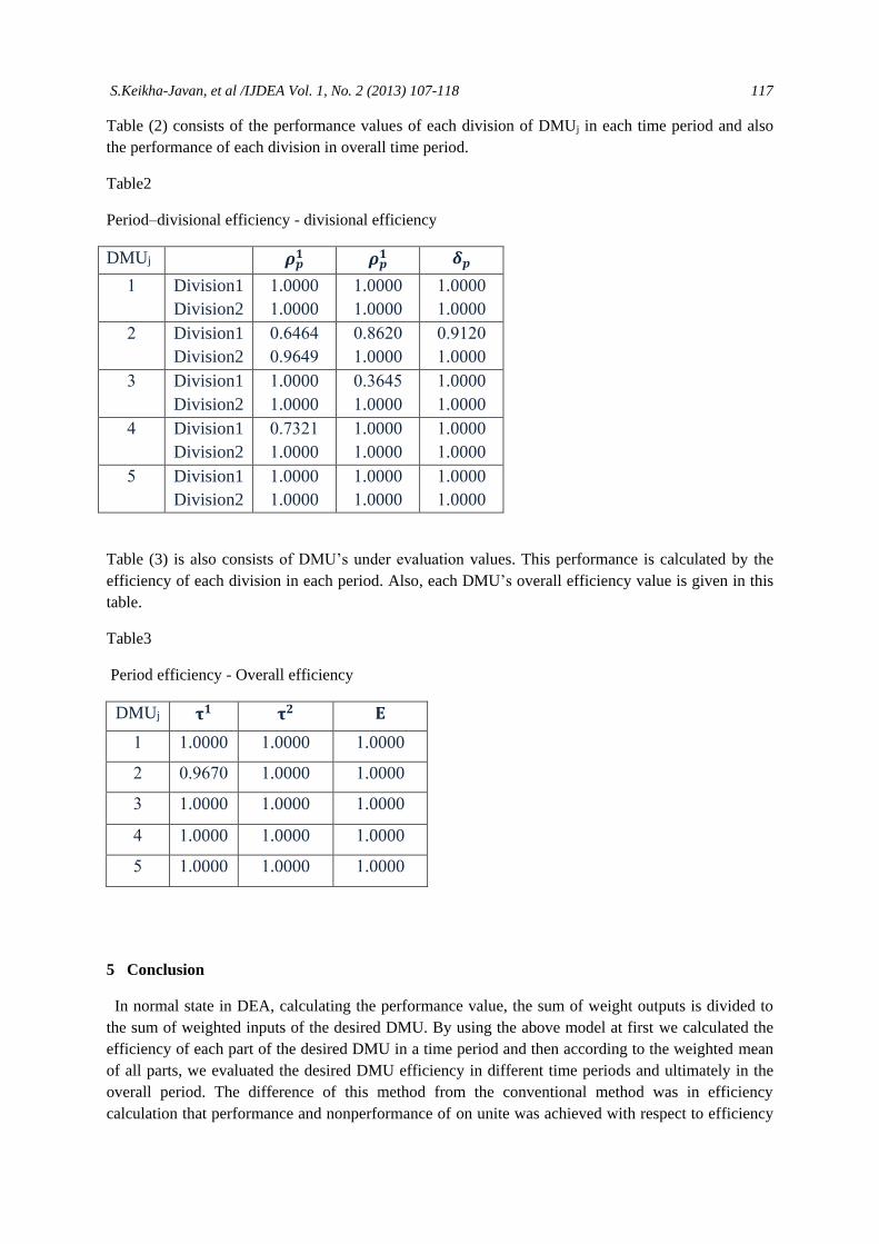
Table (2) consists of the performance values of each division of DMUj in each time period and also

the performance of each division in overall time period.

Table2

Period–divisional efficiency - divisional efficiency

𝜹𝒑 𝝆𝒑𝟏 𝝆𝒑

𝟏 DMUj

7.0000

7.0000

7.0000

7.0000

7.0000

7.0000

Division1

Division2

7

026780

7.0000

022980

7.0000

029090

026906

Division1

Division2

8

7.0000

7.0000

024907

7.0000

7.0000

7.0000

Division1

Division2

4

7.0000

7.0000

7.0000

7.0000

021487

7.0000

Division1

Division2

0

7.0000

7.0000

7.0000

7.0000

7.0000

7.0000

Division1

Division2

7

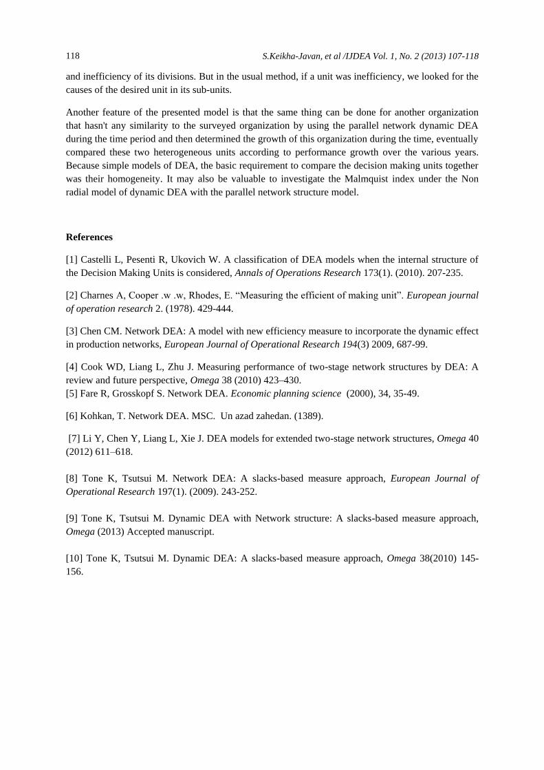
Table (3) is also consists of DMU’s under evaluation values. This performance is calculated by the

efficiency of each division in each period. Also, each DMU’s overall efficiency value is given in this

table.

Table3

Period efficiency - Overall efficiency

𝐄 𝛕𝟐 𝛕𝟏 DMUj

7.0000 7.0000 7.0000 7

7.0000 7.0000 026910 8

7.0000 7.0000 7.0000 4

7.0000 7.0000 7.0000 0

7.0000 7.0000 7.0000 7

5 Conclusion

In normal state in DEA, calculating the performance value, the sum of weight outputs is divided to

the sum of weighted inputs of the desired DMU. By using the above model at first we calculated the

efficiency of each part of the desired DMU in a time period and then according to the weighted mean

of all parts, we evaluated the desired DMU efficiency in different time periods and ultimately in the

overall period. The difference of this method from the conventional method was in efficiency

calculation that performance and nonperformance of on unite was achieved with respect to efficiency


and inefficiency of its divisions. But in the usual method, if a unit was inefficiency, we looked for the

causes of the desired unit in its sub-units.

Another feature of the presented model is that the same thing can be done for another organization

that hasn't any similarity to the surveyed organization by using the parallel network dynamic DEA

during the time period and then determined the growth of this organization during the time, eventually

compared these two heterogeneous units according to performance growth over the various years.

Because simple models of DEA, the basic requirement to compare the decision making units together

was their homogeneity. It may also be valuable to investigate the Malmquist index under the Non

radial model of dynamic DEA with the parallel network structure model.

References

[1] Castelli L, Pesenti R, Ukovich W. A classification of DEA models when the internal structure of

the Decision Making Units is considered, Annals of Operations Research 173(1). (2010). 207-235.

[2] Charnes A, Cooper .w .w, Rhodes, E. “Measuring the efficient of making unit”. European journal

of operation research 2. (1978). 429-444.

[3] Chen CM. Network DEA: A model with new efficiency measure to incorporate the dynamic effect

in production networks, European Journal of Operational Research 194(3) 2009, 687-99.

[4] Cook WD, Liang L, Zhu J. Measuring performance of two-stage network structures by DEA: A

review and future perspective, Omega 38 (2010) 423–430.

[5] Fare R, Grosskopf S. Network DEA. Economic planning science (2000), 34, 35-49.

[6] Kohkan, T. Network DEA. MSC. Un azad zahedan. (1389).

[7] Li Y, Chen Y, Liang L, Xie J. DEA models for extended two-stage network structures, Omega 40

(2012) 611–618.

[8] Tone K, Tsutsui M. Network DEA: A slacks-based measure approach, European Journal of

Operational Research 197(1). (2009). 243-252.

[9] Tone K, Tsutsui M. Dynamic DEA with Network structure: A slacks-based measure approach,

Omega (2013) Accepted manuscript.

[10] Tone K, Tsutsui M. Dynamic DEA: A slacks-based measure approach, Omega 38(2010) 145-

156.

network structure - دانشگاه آزاد اسلامی...

Documents