neural adaptive control in application service …gmagoulas/nn-control-in-asm_evos-bb.pdf · neural...

ORIGINAL PAPER

Neural Adaptive Control in Application Service ManagementEnvironment

Tomasz D. Sikora • George D. Magoulas

Received: 6 January 2013 / Accepted: 11 June 2013

� Springer-Verlag Berlin Heidelberg 2013

Abstract We introduce a learning controller framework

for adaptive control in application service management

environments and explore its potential. Run-timemetrics are

collected by observing the enterprise system during its nor-

mal operation and load tests are persisted creating a knowl-

edge base of real system states. Equipped with such

knowledge the proposed framework associates system states

and high/low service level agreement valueswith successful/

unsuccessful control actions. These associations are used to

induce decision rules, which help generating training sets for

a neural networks-based control decision module that oper-

ates in the application run-time. Control actions are executed

in the background of the current system state, which is then

again monitored and stored extending the system state

repository/knowledge base, and evaluating the correctness

of the control actions frequently. This incremental learning

leads to evolving controller behavior by taking into account

consequences of earlier actions in a particular situation, or

other similar situations. Our tests demonstrate that this

controller is able to adapt to changing run-time conditions

and workloads based on SLA definitions and is able to control

the instrumented system under overloading effectively.

Keywords Application service management � Adaptivecontroller � Service level agreement � Knowledge-basedsystems � Neural networks � Performance metrics

1 Introduction

Application service management (ASM) focuses on the

monitoring and management of performance and quality of

service in complex enterprise systems. An ASM controller

needs to react adaptively to changing system conditions in

order to optimize a set of service level agreements (SLAs),

which operate as objective functions.

High dimensionality and nonlinearities, inherent in

enterprise systems, pose several challenges to their mod-

eling and run-time control. Most of the existing research in

automating ASM is based on some kind of model. This is,

for example, expressed in the form of resources charac-

teristics, code-base structure or other system properties

which must be directly available. As discussed in Sect. 2),

automatic ASM approaches are normally able to accom-

modate a low number of dimensions. Thus, in practice,

enterprise system administrators, cloud-based solution

users or SaaS suppliers staff use manual or semi-automated

procedures that enable production level run-time modifi-

cations (Buyya et al. 2008).

In an attempt to expand automation in ASM, this paper

proposes, implements and tests an approach that is based

on autonomous control in the ASM framework, where

selected functionalities pointed to exposed, or internal,

interfaces are auto-controllable, in accordance with func-

tions of priorities in times of higher importance or lower

system resources, see an example of SLAs in Table 1. Our

approach is model-free and exploits the synergy of neural

networks and knowledge-based systems, which, to the best

of our knowledge, is innovative in this area. Moreover, our

work develops a software framework that is equipped with

simple statistical methods for evaluating the system. The

framework is able to change internal elements of runtime

execution by taking control actions in the background of

T. D. Sikora (&) � G. D. Magoulas

Department of Computer Science and Information Systems,

Birkbeck, University of London, Malet Street,

London WC1E 7HX, UK

e-mail: [email protected]

G. D. Magoulas

e-mail: [email protected]

123

Evolving Systems

DOI 10.1007/s12530-013-9089-2

p py

Table 1 Examples of SLA definitions

Attribute name SLA definition attribute value

Code/name ‘SLA1: 1$ per every extra second over 2 s execution’

SLA value phrase ‘Case when (sum(metricvalue) - 1,000)/1,000 B 60 then (sum(metricvalue) - 1,000)/1,000 else 60 end’

Summary of execution times but no more than 60$ penalty

Base resource filter ‘%//HTTP/127.0.0.1%:8081//dddsample/public/trackio [null]’

Metric value filter ‘Metricvalue C2,000’

Take into account actions longer than 2 s only

Group having phrase ‘1 = 1’—not used

Code/name ‘SLA3: 10$ for every started second of an image processing longer by average than 10 ms’

SLA value phrase ‘Ceil(10 9 (count(1) 9 sum(r.metricvalue)/1,000))’

10$ of every started second of processing—note: metrics execution time in ms

Base resource filter ‘Example filter1//HTTP/1.1://127.0.0.1(127.0.0.1):8081//dddsample/images/%’

Interprets execution time metrics of images processing on server side, filtered by a specific filter set

Metric value filter ‘1 = 1’

There is no filter on metrics values applied

Group having phrase ‘Avg(r.metricvalue) C 10’

But only those time buckets which average metric value is longer than 10 ms

Code/name ‘SLA10: 1$ per every teminated action’

SLA value phrase ‘20 9 count(1)’

20$ penalty for each of executed actions

Base resource filter ‘org.allmon.client.controller.terminator.NeuralRulesJavaCallTerminatorController.terminate’

Metric value filter ‘Exceptionbody is not null and sourcename like ’’ %.VoidLoadAdderImpl.generateIOLoad’

Checks metrics for which the filtered call was terminated with exception and source call was coming

from additional load generator method


Code/name ‘SLA50: 0.01$ price per every public call shorter than 1 s’

SLA value phrase ‘-0.01 9 count(1)’

0.01$ price an action executed

Base resource filter ‘%//HTTP/%//application/public/%%/%.do%’

Interprets all metrics of instrumented public application code

Metric value filter ‘Metricvalue B1,000’

Actions shorter than 1 s only


Code/name ‘SLA51: 50$ extra penalty per every public call longer than 3 s during peak hours’

SLA value phrase ‘50 9 count(1)’

50$ penalty for longer actions, executed from 3 to 6 pm (the business peak hours) in working days

Base resource filter ‘%//HTTP/%//application/public/%’

Interprets all metrics of instrumented public application code

Metric value filter ‘Metricvalue C3,000’ and to_char(timestamp, ‘HH24’) in (‘15’, ‘16’, ‘17’) and to_char(timestamp, ‘D’) B5’

Actions longer than 2 s only

Group having phrase ‘Count(1) C100’

SLA values are calculated only in times when more than 100 action calls executed per time bucket

Evolving Systems

123

p py

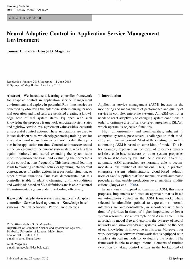
flexible SLA definitions, available resources, and system

states. An overview of the framework is illustrated in

Fig. 1.

In the era of ‘‘big-data’’ (Brown et al. 2011; Buyya et al.

2008) we use an approach where all metrics are collected,

e.g. relating to performance of resources and control actions,

thus creating a knowledge base that also operates as a

repository of system states and reactions to particular control

actions. In this paper we focus on an enterprise application

where the controller is only equipped with a termination

actuator eliminating expensive actions (not resources tun-

ing1), and can adapt to changing conditions according to

modifiable SLA definitions, still without a model of the

system. No predictors and no forecasting of service demands

and resources utilization have been used. The general

objective is to optimize declared SLA functions values.

The paper is organized as follows. Section 2 presents

previous work in the ASM domain—the various control

schemes proposed so far and their advantages and limita-

tions. Section 3 introduces important research concepts and

defines the terminology used. Section 4 formulates the

problem and our approach. Section 5 introduces and dis-

cusses the architecture of the proposed framework used to

monitor and control an application. Section 6 presents

experimental results. Section 7 contains conclusions and

discusses future research.

2 Previous work in ASM control

The adaptive control of services has been the subject of

substantial focus in the last decade. Parekh et al. (2002)

were researching the area of adaptive controllers using

control theory and standard statistical models. More

pragmatic approaches were studied in Abdelzaher and Lu

(2000), Abdelzaher et al. (2002), Zhang et al. (2002a, b),

Lu et al. (2002, 2003), Abdelzaher et al. (2003), where

an ASM performance control system with service dif-

ferentiation was using classical feedback control theory

to achieve overload protection. Hellerstein and Parekh

et al. introduced a comprehensive application of standard

control theory to describe the dynamics of computing

systems and apply system identification to the ASM field

(Hellerstein et al. 2004), highlighting engineering chal-

lenges and control problems (Hellerstein 2004). Fuzzy

control and neuro-fuzzy control were proposed in Hel-

lerstein et al. (2004) as promising for adaptive control in

the ASM field, which may also be an interesting area for

further research work.

Since then many different methods of control and var-

ious techniques for actuators in ASM have been proposed

e.g., adaptive admission control as dynamic service over-

load management protection (Welsh and Culler 2002),

event queues for response times of complex Internet ser-

vices (Welsh and Culler 2003), autonomic buffer pool

configuration in a DB level (Powley et al. 2005), model

approximation and predictors with SLA specification for

different operation modes (Abrahao et al. 2006), observed

output latency and a gain controller for adjusting the

number of servers (Bodık et al. 2009).

The notion of SLA, as a concept based on quality of

service (QoS), is widely adopted in the business (Park et al.

2001). SLA definitions are often used in Cloud and Grid

computing control (Vaquero et al. 2008; Buyya et al. 2009;

Patel et al. 2009; Stantchev and Schropfer 2009). Thus,

more recent works in this area tend to focus on perfor-

mance control in more distributed environments, e.g. vir-

tualized environments performance management, Xiong

et al. (2010), virtualized server loopback control of CPU

allocation to multiple applications components to meet

response time targets (Wang et al. 2009). Cloud based

Fig. 1 ASM control process

life-cycle (starting from the top

clockwise). a Monitoring of

resources available and

application activity, b SLA

processing, c metrics

persistence, d evaluating control

and rules generation, e applyingcontrol

1 The system resources can be modified in order to change important

run-time characteristics—this scenario is not discussed in this paper.

Evolving Systems

123

p py

solutions with QoS agreements services were researched by

Boniface et al. (2010) and Sun et al. (2011), where multi-

dimensional QoS cloud resource scheduling with use of

immune clonal was researched. An interesting work by

Emeakaroha et al. (2010) presents cloud environment

control with the use of a mapping from monitored low-

level metrics to high-level SLA parameters. Power man-

agement by an on-line adaptive ASM system was resear-

ched in Kandasamy et al. (2004), Kusic et al. (2009), and

energy saving objectives and effective cooling in data

centers in Chen et al. (2010), Bertoncini et al. (2011).

Although autonomous control in ASM environments

still needs substantial research to be conducted, manual

ASM administration is widely used, together with the

deployment of application performance management

(APM) tools. Currently there are many out-of-the-shelf

APM and ASM suites (Kowall and Cappelli 2012), mainly

focusing on network and operating system resources

monitoring.

Despite the recent progress in the use of control theory

to design controllers for ASM, the use of neural networks

and their ability to approximate multidimensional functions

defining control actions in system states remains under

explored. Bigus nearly twenty years ago applied neural

networks and techniques from control systems to system

performance tuning (Bigus 1994). Similarly to our

approach he used several system performance measures,

such as devices utilization, queue lengths, and paging rates.

Data were collected to train neural network performance

models. For example, NNs were trained on-line to adjust

memory allocations in order to meet declared performance

objectives. Bigus et al. (2000) extended that approach and

proposed a framework for adjusting resources allocation,

where NNs were used as classifiers and predictors, but no

extensive knowledge base was incorporated in that

approach.

In contrast to previous attempts, no enterprise system

model of any kind is present in our approach, and a

knowledge base is incorporated to store system metrics

and control actions. This allows us to persist all the

metrics and SLA values before any control action is

applied, and then reevaluate these control actions in line

with evolving system characteristics and retrain neural

networks to implement new control rules on-line. Such

evaluation of control actions does not require setting

directly control actions according to defined and delivered

SLAs. Also in terms of SLAs, our approach provides a

flexible way of defining functions, allowing the selection

and combination of all metrics present in the knowledge

base. Lastly, in this study we employ neural termination

actuators weaved in the application under control, which

is an approach that has not been explored in the ASM

field adequately.

3 Concepts and definitions

This section introduces research concepts and defines ter-

minology used later in the paper. The mathematical nota-

tion, the analysis of the considered dimensions and the

system state definitions presented here will be used in the

problem statement described later in Sect. 4.

Let us define a system of functions:

C : Rnþ1 ! Rnþ1; n ¼ k þ m in time domain, where k is

the number of measurable system actions and m is the

number of system resources. All run-time characteristics of

the enterprise system are defined by a set of resources and

input/output actions, whose current values define the sys-

tem state S:

Let us assume that r is the set of all system resources,

which fully describe the system conditions. We will mainly

focus on those resources which are measurable r ¼fr1; . . .; ri; . . .; rmg; r � r; where the i-th resource utiliza-

tion is a scalar function of other measurable resources and

actions in time riðtÞ ¼ qðr; a; tÞ; riðtÞ 2 ½0;1�: Only some

measurable system resources can be controllable rc � r:

There are synthetic resources (abstract resources), which

can be derived/calculated on the basis of other system

parameters (resources and actions functions) rs � r ^ rs \rc ¼ ; : rsðtÞ ¼ qsðrðtÞ; aðtÞÞ; therefore they cannot be

controlled directly but can be used in later processing for

control rules induction.

Let us assume that a is the set of all system actions, we

focus on only measurable actions (assuming that not all

actions can be monitored) a ¼ fa1; . . .; ai; . . .; akg; a � a;

where the i-th action execution is a function of resources

utilized aiðtÞ ¼ aðr; a; ciðtÞ;PiÞ; aiðtÞ 2 f0; 1g that is trig-

gered by the i-th event impulse with vector input parame-

ters Pi ¼ ½P1; . . .;PX�;Pi 2 RX ; which depends on

available system resources and, consequently, on other

actions executions, i.e. aðPiÞi ðtÞ ¼ aðr; a; tÞ: Similarly to

resources definitions, some actions are controllable ac � a:

The controller2 can readjust execution time character-

istics during actions run-time, including termination, but is

not allowed to change other functionalities. Many instances

of the same action type can execute concurrently, i.e. the i-

th action type can have many instances executing concur-

rently for different values of the input parameters Pi:

In this context, an important concept is the service level

agreement (SLA). In most cases this is considered as a

monotonic function of actions, resources and time

2 The term controller is used as a name of a function of the proposed

framework. Due to distributed nature of the framework and the lack of

a model of the enterprise system, the function is split into two

software components and is deployed in isolation, see Sects. 5.4 and

5.6, where the evaluator, which generates control rules by learning

from available data, and the controller API, which coordinates work

of actuator agents, are described.

Evolving Systems

123

p py

fSLAi¼ fSLAi

ða; r; tÞ; t 2 R: Very often SLAs are functions

of an action’s execution time but can be also built as

functions of expensive system resources used. Also

9tr2RfSLA [ 0 ^ 9tp2RfSLA\0; are reward and penalty con-

ditions respectively. More concrete SLAs definitions

examples are presented in Table 1.

Lastly, the System model C; as a vector of functions

describing the system state space in discrete time domain

C : ½r; a�; can be also presented as the following system of

difference equations (state space), containing often highly

non-linear functions riðtÞ 2 r; aiðtÞ 2 a:

C :

r1ðtÞ...

rmðtÞ; rðtÞ ¼ qðrðt � 1Þ; aðPiÞðt � 1Þ; tÞ;a1ðtÞ aðtÞ ¼ aðrðt � 1Þ; aðPiÞðt � 1Þ; tÞ...

akðtÞ

8>>>>>>>><>>>>>>>>:

ð1Þ

4 Problem statement

In this section we describe the problem under consideration

and provide an overview of the proposed approach.

4.1 The control problem

An enterprise class system architectures can vary sub-

stantially depending on functionality, interconnections to

other system, and other non-functional requirements. There

can be many different components and software tiers

present, which consist internal and externals services calls,

according to implemented routines. Typically the system

can host hundreds to thousands exposed system actions,

and be described by hundreds of software and hardware

resources depending on deployment redundancy (Haines

2006; Grinshpan 2012). Moreover many characteristics

may change in time due to load changes, further develop-

ment functional modifications, or other technical

interventions.

In order to optimize an enterprise system under load, the

control system must consider not only the current state of

the system S; but it also must be instructed on the direction

of the changes to be applied.

In this work the objective functions are defined in the

form of a list of SLAs. The controller should keep the

cumulative SLA values minimal under changing condi-

tions. Only specified controllable actions ac can be termi-

nated. Such an online adaptive control scheme should be

able to operate in a complex multidimensional space of

input measurements, observed output dimensions, and

nonlinear system dynamics (Hellerstein et al. 2004), where

the relations between the various dimensions are hidden.

It is difficult to build a control model of a system, where

crucial run-time properties are unknown. Therefore the

main feature of our approach is that it considers the

enterprise system as a black-box: it uses no explicit or

analytic model of the system. In particular there is no direct

knowledge of the code-base structure and characteristics of

the resources. We do not apply any predictors, nor build

statistical models for the distributions of run-time dimen-

sions. Therefore, the control system has to constitute future

control actions by observing system states S and their

changes. It learns by observing, storing metrics, searching

similarities from the past, and enhancing concrete control

solutions of this optimization problem by applying evalu-

ation of the control actions.

4.2 Induction of control rules

The control system ‘‘learns by observation’’, building a

Knowledge Base and solving the optimization problem

under SLA definitions. This type of ‘‘learning’’ is in

essence a very natural process as Thorndike discovered

while researching animals adaptation facing pleasant and

unpleasant situations (Thorndike and Bruce 1911; Herrn-

stein 1970). This was later extended in the work of Skinner

in the area of operant conditioning and defined principles

of reinforcement and behaviorism (Skinner 1938, 1963),

which influenced research in machine learning for control

by reward and punishment (Watkins 1989; Sutton 1984;

Sutton and Barto 1998).

The idea of exploiting background knowledge with

positive and negative examples in order to formulate a rule-

based hypothesis about the accuracy of an action was

researched in the context of inductive reasoning (Muggle-

ton and De Raedt 1994; Muggleton 1999), giving grounds

of Inductive logic programming.

We use a reward and punishment method in order to

learn and represent control rules according to the specified

in SLAs direction, as explained in more details below.

4.3 The control approach

In this work an approach that builds on the above men-

tioned schemes is applied, where system states associated

with low SLA values are promoted and those which lead to

high SLA penalty values are discouraged in future con-

troller actions. In order to promote this behavior, an on-line

adaptation procedure through frequent evaluations is per-

formed. A search is executed for each of the process runs to

uncover new and evaluate existing associations (indirect

mappings) between system states and SLA values. So the

problem space of unknown yet possible application system

states of observable dimensions of C : ½r; a� is being con-

stantly explored. Generally this sort of trial and error

Evolving Systems

123

p py

method works quite well, where little a priori knowledge is

available.

As mentioned earlier, the control system is able to

modify only a subset of all functional actions ac, those

which are expressly instrumented with the controller agents

code. A control action in a given system state caðSÞ is a

direct result of a rule induced RðSÞ; approximated with use

of neural networks.

When induced, a control rule is a type of belief

(expectation) that in the background of a system state S; in

an area of observable dimensions (a, r), the applied control

is going to lead to a lower SLA value. When the rule is

applied in the system, a new state is observed that extends

the system state repository, reflecting the correctness of the

control action. More details of the rules induction process

are presented in Sect. 5.4.

In this paper we treat SLAs as penalties of equal

importance. Following this assumption a summary of all

set SLAs can be computed in order to derive knowledge

about the system’s ‘‘health’’. The control can be applied on

the basis of rules induced under this assumption.

5 Proposed framework and controller architecture

In this section wewill be describing the proposed framework

and its various elements, such as the monitoring mechanism

and the controller architecture. We will also discuss various

components of the environment used for simulations and

practical evaluation of the proposed solution.

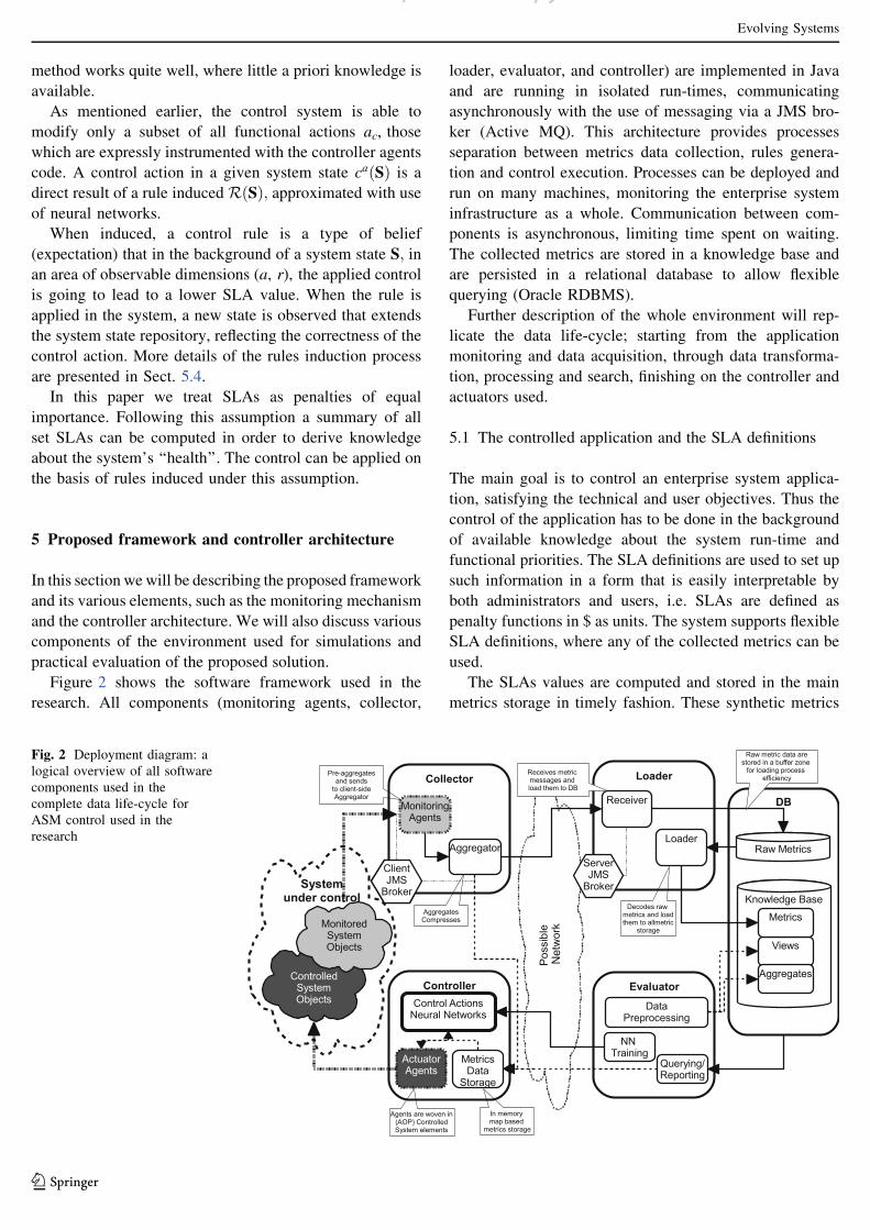
Figure 2 shows the software framework used in the

research. All components (monitoring agents, collector,

loader, evaluator, and controller) are implemented in Java

and are running in isolated run-times, communicating

asynchronously with the use of messaging via a JMS bro-

ker (Active MQ). This architecture provides processes

separation between metrics data collection, rules genera-

tion and control execution. Processes can be deployed and

run on many machines, monitoring the enterprise system

infrastructure as a whole. Communication between com-

ponents is asynchronous, limiting time spent on waiting.

The collected metrics are stored in a knowledge base and

are persisted in a relational database to allow flexible

querying (Oracle RDBMS).

Further description of the whole environment will rep-

licate the data life-cycle; starting from the application

monitoring and data acquisition, through data transforma-

tion, processing and search, finishing on the controller and

actuators used.

5.1 The controlled application and the SLA definitions

The main goal is to control an enterprise system applica-

tion, satisfying the technical and user objectives. Thus the

control of the application has to be done in the background

of available knowledge about the system run-time and

functional priorities. The SLA definitions are used to set up

such information in a form that is easily interpretable by

both administrators and users, i.e. SLAs are defined as

penalty functions in $ as units. The system supports flexible

SLA definitions, where any of the collected metrics can be

used.

The SLAs values are computed and stored in the main

metrics storage in timely fashion. These synthetic metrics

Fig. 2 Deployment diagram: a

logical overview of all software

components used in the

complete data life-cycle for

ASM control used in the

research

Evolving Systems

123

p py

extend the knowledge base. Typically the standard time

aggregation is used, so the scalar values are stored per time

bucket.

SLA definitions in the current implementation use SQL

phrases, as this method was found as a very flexible way of

specifying the run-time and the business situations. An

example is provided below

More examples of SLAs can be found in Table 1. The

first three SLA definitions have been used in the simula-

tions explained later. The last two examples define a

business scenario SLAs, showing a more practical use. The

engine is very flexible, so administrators can easily join all

metric values collected in the metrics database. Also, ser-

vice providers would have an option of flexible pricing,

which is often limited to flat rates or tariffs based on

exposed functionality usage thresholds.

5.2 The application monitoring environment

All data for the metrics are acquired from monitored parts

of a system by remote agents. The monitoring framework3

utilized passive and active monitoring as complementary

techniques of performance tracking in distributed systems.

Active (Synthetic) monitoring collects data in scheduled

mode by scripts, which often simulate an end-user activity.

Those scripts continuously monitor at specified intervals,

for performance and availability reasons, various system

metrics. Active agents are also used to gather information

about resource states in the system. Active monitoring is

applied whenever there is a strong need to gather infor-

mation about the current state of the application, and to

detect easily times of lower or higher than normal activity.

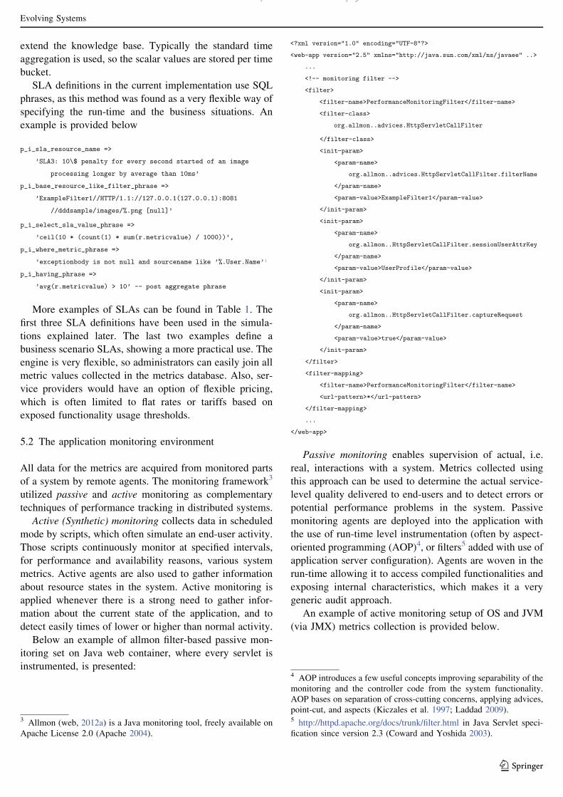
Below an example of allmon filter-based passive mon-

itoring set on Java web container, where every servlet is

instrumented, is presented:

Passive monitoring enables supervision of actual, i.e.

real, interactions with a system. Metrics collected using

this approach can be used to determine the actual service-

level quality delivered to end-users and to detect errors or

potential performance problems in the system. Passive

monitoring agents are deployed into the application with

the use of run-time level instrumentation (often by aspect-

oriented programming (AOP)4, or filters5 added with use of

application server configuration). Agents are woven in the

run-time allowing it to access compiled functionalities and

exposing internal characteristics, which makes it a very

generic audit approach.

An example of active monitoring setup of OS and JVM

(via JMX) metrics collection is provided below.

3 Allmon (web, 2012a) is a Java monitoring tool, freely available on

Apache License 2.0 (Apache 2004).

4 AOP introduces a few useful concepts improving separability of the

monitoring and the controller code from the system functionality.

AOP bases on separation of cross-cutting concerns, applying advices,

point-cut, and aspects (Kiczales et al. 1997; Laddad 2009).5 http://httpd.apache.org/docs/trunk/filter.html in Java Servlet speci-

fication since version 2.3 (Coward and Yoshida 2003).

Evolving Systems

123

p py

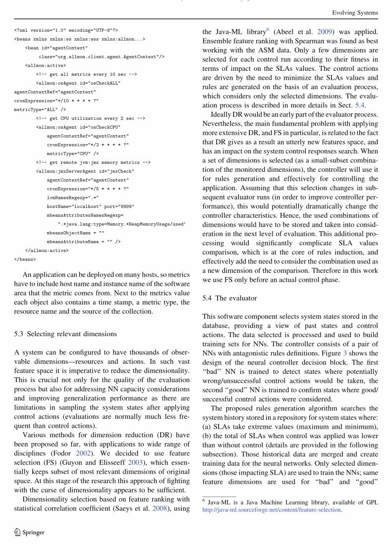
An application can be deployed onmany hosts, so metrics

have to include host name and instance name of the software

area that the metric comes from. Next to the metrics value

each object also contains a time stamp, a metric type, the

resource name and the source of the collection.

5.3 Selecting relevant dimensions

A system can be configured to have thousands of obser-

vable dimensions—resources and actions. In such vast

feature space it is imperative to reduce the dimensionality.

This is crucial not only for the quality of the evaluation

process but also for addressing NN capacity considerations

and improving generalization performance as there are

limitations in sampling the system states after applying

control actions (evaluations are normally much less fre-

quent than control actions).

Various methods for dimension reduction (DR) have

been proposed so far, with applications to wide range of

disciplines (Fodor 2002). We decided to use feature

selection (FS) (Guyon and Elisseeff 2003), which essen-

tially keeps subset of most relevant dimensions of original

space. At this stage of the research this approach of fighting

with the curse of dimensionality appears to be sufficient.

Dimensionality selection based on feature ranking with

statistical correlation coefficient (Saeys et al. 2008), using

the Java-ML library6 (Abeel et al. 2009) was applied.

Ensemble feature ranking with Spearman was found as best

working with the ASM data. Only a few dimensions are

selected for each control run according to their fitness in

terms of impact on the SLAs values. The control actions

are driven by the need to minimize the SLAs values and

rules are generated on the basis of an evaluation process,

which considers only the selected dimensions. The evalu-

ation process is described in more details in Sect. 5.4.

IdeallyDRwould be an early part of the evaluator process.

Nevertheless, the main fundamental problem with applying

more extensive DR, and FS in particular, is related to the fact

that DR gives as a result an utterly new features space, and

has an impact on the system control responses search. When

a set of dimensions is selected (as a small-subset combina-

tion of the monitored dimensions), the controller will use it

for rules generation and effectively for controlling the

application. Assuming that this selection changes in sub-

sequent evaluator runs (in order to improve controller per-

formance), this would potentially dramatically change the

controller characteristics. Hence, the used combinations of

dimensions would have to be stored and taken into consid-

eration in the next level of evaluation. This additional pro-

cessing would significantly complicate SLA values

comparison, which is at the core of rules induction, and

effectively add the need to consider the combination used as

a new dimension of the comparison. Therefore in this work

we use FS only before an actual control phase.

5.4 The evaluator

This software component selects system states stored in the

database, providing a view of past states and control

actions. The data selected is processed and used to build

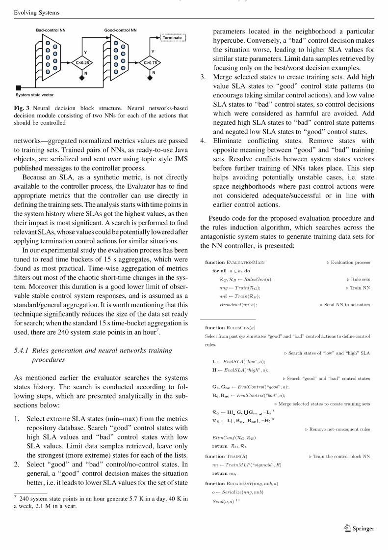
training sets for NNs. The controller consists of a pair of

NNs with antagonistic rules definitions. Figure 3 shows the

design of the neural controller decision block. The first

‘‘bad’’ NN is trained to detect states where potentially

wrong/unsuccessful control actions would be taken, the

second ‘‘good’’ NN is trained to confirm states where good/

successful control actions were considered.

The proposed rules generation algorithm searches the

system history stored in a repository for system states where:

(a) SLAs take extreme values (maximum and minimum),

(b) the total of SLAs when control was applied was lower

than without control (details are provided in the following

subsection). Those historical data are merged and create

training data for the neural networks. Only selected dimen-

sions (those impacting SLA) are used to train the NNs; same

feature dimensions are used for ‘‘bad’’ and ‘‘good’’

6 Java-ML is a Java Machine Learning library, available of GPL

http://java-ml.sourceforge.net/content/feature-selection.

Evolving Systems

123

p py

networks—ggregated normalized metrics values are passed

to training sets. Trained pairs of NNs, as ready-to-use Java

objects, are serialized and sent over using topic style JMS

published messages to the controller process.

Because an SLA, as a synthetic metric, is not directly

available to the controller process, the Evaluator has to find

appropriate metrics that the controller can use directly in

defining the training sets. The analysis startswith timepoints in

the system history where SLAs got the highest values, as then

their impact is most significant. A search is performed to find

relevant SLAs,whosevalues couldbepotentially loweredafter

applying termination control actions for similar situations.

In our experimental study the evaluation process has been

tuned to read time buckets of 15 s aggregates, which were

found as most practical. Time-wise aggregation of metrics

filters out most of the chaotic short-time changes in the sys-

tem. Moreover this duration is a good lower limit of obser-

vable stable control system responses, and is assumed as a

standard/general aggregation. It is worth mentioning that this

technique significantly reduces the size of the data set ready

for search; when the standard 15 s time-bucket aggregation is

used, there are 240 system state points in an hour7.

5.4.1 Rules generation and neural networks training

procedures

As mentioned earlier the evaluator searches the systems

states history. The search is conducted according to fol-

lowing steps, which are presented analytically in the sub-

sections below:

1. Select extreme SLA states (min–max) from the metrics

repository database. Search ‘‘good’’ control states with

high SLA values and ‘‘bad’’ control states with low

SLA values. Limit data samples retrieved, leave only

the strongest (more extreme) states for each of the lists.

2. Select ‘‘good’’ and ‘‘bad’’ control/no-control states. In

general, a ‘‘good’’ control decision makes the situation

better, i.e. it leads to lower SLA values for the set of state

parameters located in the neighborhood a particular

hypercube. Conversely, a ‘‘bad’’ control decision makes

the situation worse, leading to higher SLA values for

similar state parameters. Limit data samples retrieved by

focusing only on the best/worst decision examples.

3. Merge selected states to create training sets. Add high

value SLA states to ‘‘good’’ control state patterns (to

encourage taking similar control actions), and low value

SLA states to ‘‘bad’’ control states, so control decisions

which were considered as harmful are avoided. Add

negated high SLA states to ‘‘bad’’ control state patterns

and negated low SLA states to ‘‘good’’ control states.

4. Eliminate conflicting states. Remove states with

opposite meaning between ‘‘good’’ and ‘‘bad’’ training

sets. Resolve conflicts between system states vectors

before further training of NNs takes place. This step

helps avoiding potentially unstable cases, i.e. state

space neighborhoods where past control actions were

not considered adequate/successful or in line with

earlier control actions.

Pseudo code for the proposed evaluation procedure and

the rules induction algorithm, which searches across the

antagonistic system states to generate training data sets for

the NN controller, is presented:

Fig. 3 Neural decision block structure. Neural networks-based

decision module consisting of two NNs for each of the actions that

should be controlled

7 240 system state points in an hour generate 5.7 K in a day, 40 K in

a week, 2.1 M in a year.

Evolving Systems

123

p py

In order to provide concise description more detailed

comments of the above pseudocode were moved to foot-

notes8, 9, 10, 11, 12, 13, 14, 15

5.4.2 Extrema search and previous control actions

High SLA values based on actions execution time can be a

result of utilized resources saturation. Moreover, some of

the SLAs values could be more expensive than violations

of SLAs due to terminated actions. The precise situation

depends, of course, on the SLAs definitions as well as on

the enterprise system’s load and the quantity of potential

violations. In most practical cases, however, termination

actions can have an impact on SLAs that depend on action

execution time. The termination actuator can release load

and effectively lower SLA values. This approach promotes

termination of actions for a system state associated with the

highest SLA footprint, and condemns termination decisions

that caused more harm than benefit in terms of SLA levels.

Previous control actions stored in the repository, are

compared according to summary of SLAs for a given

system state S: As noted above only the best and the worst

control actions are considered. The size of the set c is

tunable and typically depends linearly on the number of

dimensions selected, and the total number of the system

states in the repository.

It is worth mentioning here an interesting effect. There

is possibility to change the SLA definitions while the

control system operates. Although there is no technical

problem to recalculate new SLA values, as past system

states are available, it is not possible to evaluate all reac-

tions to control decisions, as such modification could fun-

damentally change the dynamics of the control system. A

similar problem was described earlier in Sect. 5.3, where

impacts of frequent dimensions selection and effective

system space search were noted.

5.4.3 Conflict resolving strategies

Strategies for conflict resolution were introduced in order

to deal with a problem of inducing potentially not conse-

quent rules that could lead to poor response to control

actions, and good/bad rule sets RG;RB that may contain

conflicting directives for similar system state S : SG � SB:

Similarity criteria used here are based on Chebyshev

distance in the normalized metrics data space, so a

hypercube shape neighborhood is considered. Thus, two

states are similar SG � SB when the following similarity

condition holds: 8ðdG2SG; dB2SBÞjdG � dBj\n:In other words, the Chebyshev distance DCh(p, q) :=

maxi(|pi - qi|) between system states is lower than the

neighborhood distance DChðSG; SBÞ\n: The neighborhooddistance n is tunable, but normally is set to 5 % of a

dimension range.

Initially, all similar system states from both ‘‘good’’ and

‘‘bad’’ sets of rules were removed in order to avoid

8 Merge sets of states of high SLA values and ‘‘good’’ control to

promote these control actions.9 Merge sets of states of low SLA values and ‘‘bad’’ controlto prevent

harmful control decisions.10 Trained networks are sent to the controller actuators, sothey are

directly available in the controlled application run-time.11 Select m system states S of highest SLAs for ‘‘good’’ control

states, where penalties for the control SLApca (S) werelower than total

of SLAs in the state neighborhood.12 Select m states of lowest SLAs for ‘‘bad’’ control states,where

penalties for the control SLApca (S) were higher thanSLAs (too harmful

control)—these rules instruct to avoidapplying any control in such

states.13 A ‘‘good’’ control decision is the one that makes the situation

better, so select system states S where total of SLAsis lower for

similar state parameters.14 A ‘‘bad’’ control decision is the one that makes the situation worse,

so select states where SLAs are higher for similarstate parameters.15 In the simplest form both system states are removed.There have

been more variants of resolving conflicts researched as well.

Evolving Systems

123

p py

conflicts—this strategy is named Variant A. This was

found too strict, in the sense that too many data points were

removed when adopting this strategy. Training sets for

NNs appear often degenerated and poor-in-value during

simulations when too many contradicting rules are gener-

ated in the same states neighborhood. In our experiments,

this scenario mainly occurred at the start of the controller

operation, or when the run-time situation changed

drastically.

Therefore slightly more advanced algorithms for pre-

venting rule conflicts are suggested. In order to implement

these strategies the system state vector has to be extended

with additional measures, calculated from data points

within the system state neighborhood, such as the total of

SLA values, the count of similar system states (cardinal-

ity), the average of SLA values. That leads to the following

set of strategies:

– Variant A—this is a very strict strategy that eliminates

all system states if they lay in the same neighborhood.

– Variant B—this strategy adopts a simple approach

checking the cardinality of similar rules induced in the

same system state neighborhood. This variant empha-

sizes frequently occurring events, named ‘‘habits’’, and

only eliminates less frequent states, i.e. those of lower

cardinality which possess less occurring instances.

Thus, overall fewer states are eliminated compared to

Variant A.

– Variant C—this strategy eliminates system states that

lay in the same neighborhood keeping the ones that

possess higher average of SLA penalties. So the level

of SLA violations influences conflict resolution as this

strategy emphasizes high penalty events, named

‘‘trauma’’, which may be rare but significant from

SLA perspective.

A comparison of the controller behavior using above

strategies is included in the experimental part of the work

in Sect. 6.2.3.

5.5 Training set generation and rules induction

implementation

To approximate the discovered control rules by training

NNs, a simple hierarchical approach has been used. Fig-

ure 3 provides an overview of the neural networks-based

controller, discussed earlier. Each of the controlled actions

(implemented as a java class.method, servlet, etc.) has its

own dedicated pair of NNs instances which are trained to

produce control decisions depending on system states

conditions and past experiences. The NNs are trained with

‘‘bad’’ and ‘‘good’’ control action sets selected from a

repository of system history. The controller first considers

decisions of the ‘‘bad’’ network and if the current state does

not trigger any patterns learned by the NNs, then it begins

checking the ‘‘good’’ control actions.

NN are trained with normalized data, within min/max

boundaries; system state values which are exceeding the

declared scope are not taken into account by the controller,

so no control decision is taken. Of course such a situation is

monitored and when occurs it extends the boundaries in the

next evaluation iteration.

The Neuroph16 library with multi layer perceptron

implementation and sigmoid activations was applied.

Experimentally, it was found that for the proposed

training set structure, NNs with two hidden layers of four

neurons trained with the Momentum Backpropagation

algorithm, worked well in most situations. Activation

thresholds for termination actions in the control decision

module were set to 0.25 and 0.75 for ‘‘bad’’ and ‘‘good’’

control actions respectively, as shown in Fig. 3.

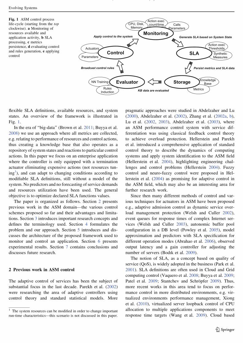
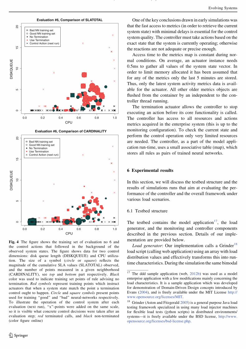
An example of rules induced, in the form of NN training

data and actual control actions are presented in Fig. 4. Two

main aspects of the rules induction and NN training sets for

the control are highlighted: (a) target NN in the decision

block—denoted by a circular or squared shape, and

(b) termination action—denoted by use of black or red

color. Thus, circles represent actions of the ‘‘good’’ neural

network, while squares denote actions of the ‘‘bad’’ net-

work. Target neural networks are trained with termination

and no-termination actions states. For example, light red

shapes indicate supported termination control, whilst black

shapes promote no control actions.

Figure 4 depicts also a comparison of total of SLA

values (top) and cardinality (bottom) of each of the system

states identified in the rule set. The size of a shape indicates

the magnitude of the SLAs values or the Cardinality in a

given system state. Crosses indicate real system states

where the neural networks-based decision module was

checked in order to decide on a particular control action to

be taken.

5.6 Controller and actuator agents

Actuator agents are weaved into an application (analogous

to passive monitoring). The controller receives serialized

trained NN instances from the evaluator process that are

stored in memory for easy and fast access by actuator APIs

before each of the controlled actions calls. To minimize the

time spent on accessing the structure a map, as a data

container, has been used.

16 Neuroph 2.4 is an open source Java neural network framework

http://neuroph.sourceforge.net/. It contains run-time level reference to

another NN library, called Encog http://code.google.com/p/encog-

java/. Both of them are published under Apache 2.0 license Apache

(2004).

Evolving Systems

123

p py

One of the key conclusions drawn in early simulations was

that the fast access to metrics (in order to retrieve the current

system state) with minimal delays is essential for the control

system quality. The controller must take actions based on the

exact state that the system is currently operating; otherwise

the reactions are not adequate or precise enough.

Access time to the metrics map is constant during nor-

mal conditions. On average, an actuator instance needs

0.5ms to gather all values of the system state vector. In

order to limit memory allocated it has been assumed that

for any of the metrics only the last 5 minutes are stored.

Thus, only the latest system activity metrics data is avail-

able for the actuator. All other older metrics objects are

flushed from the container by an independent to the con-

troller thread running.

The termination actuator allows the controller to stop

executing an action before its core functionality is called.

The controller has access to all resources and actions

metrics acquired in the enterprise system (this is up to the

monitoring configuration). To check the current state and

perform the control operation only very limited resources

are needed. The controller, as a part of the model appli-

cation run-time, uses a small associative table (map), which

stores all rules as pairs of trained neural networks.

6 Experimental results

In this section, we will discuss the testbed structure and the

results of simulations runs that aim at evaluating the per-

formance of the controller and the overall framework under

various load scenarios.

6.1 Testbed structure

The testbed contains the model application17, the load

generator, and the monitoring and controller components

described in the previous section. Details of our imple-

mentation are provided below.

Load generator: Our implementation calls a Grinder18

load script (calling web application) using an array with load

distribution values and effectively transforms this into run-

time characteristics. During the simulation the same bimodal

0.0 0.2 0.4 0.6 0.8 1.0

05

1015

20Evaluation #6, Comparison of SLATOTAL

CPU

DIS

KQ

UE

UE

Bad NN training setGood NN training setNo TerminationUse TerminationControl Action (next run)

0.0 0.2 0.4 0.6 0.8 1.0

05

1015

20

Evaluation #6, Comparison of CARDINALITY

CPU

DIS

KQ

UE

UE

Bad NN training setGood NN training setNo TerminationUse TerminationControl Action (next run)

Fig. 4 The figure shows the training set of evaluation no 6 and

the control actions that followed in the background of the

observed system states. The figure shows data for two control

dimensions: disk queue length (DISKQUEUE) and CPU utiliza-

tion. The size of a symbol (circle or square) reflects the

magnitude of the cumulative SLA values (SLATOTAL) observed,

and the number of points measured in a given neighborhood

(CARDINALITY), see top and bottom part respectively. Black

color was used to indicate training set points of rule advising no

termination. Red symbols represent training points which instruct

actuators that when a system state match the point a termination

control ought to happen. Circle and square symbols present points

used for training ‘‘good’’ and ‘‘bad’’ neural-networks respectively.

To illustrate the operation of the control system after each

evaluation (next run), ‘‘x’’-points were added on the same scale,

so it is visible what concrete control decisions were taken after an

evaluation step; red terminated calls, and black non-terminated

(color figure online)

17 The ddd sample application (web, 2012b) was used as a model

enterprise application with a few modifications mainly concerning the

load characteristics. It is a sample application which was developed

for demonstration of Domain-Driven Design concepts introduced by

Evans (2004), and is freely available under the MIT License http://

www.opensource.org/licenses/MIT.18 Grinder (Aston and Fitzgerald 2005) is a general purpose Java load

testing framework specialized in using many load injector machines

for flexible load tests (jython scripts) in distributed environments/

systems—it is freely available under the BSD license, http://www.

opensource.org/licenses/bsd-license.php.

Evolving Systems

123

p py

load pattern was used, executed consecutively many times,

in two subsequent phases with different load-levels: the first

phase had a load of ten running threads while the second had

a 20-threads load. The aim of this testing to explore how the

controller changes termination action characteristics adapt-

ing to different system conditions.

Monitored resources and actions: During this exercise

only operating system-OS resources and system response

times were monitored. Therefore only OS and system

actions metrics were included in the system state vectors.

Actions were monitored by http filter agents (no direct java

code instrumentation). The load generator calls only one

jsp page /public/trackio (?static assets pointed to it). The

page has been extended with a block with high IO intensive

code (what is consequently causing significant CPU utili-

zation). In a situation where all resources are available the

code to execute takes from 100 to 1,100 ms with uniform

distribution, but it rises significantly when used resources

are entering into a saturation state, see Fig. 5.

Controlled actions: The model application action /public/

trackio contains an object where a termination control actu-

atorwas directlywoven in.A termination exception is thrown

in situations when the neural decision block (see Fig. 3)

associates the current system state with a termination action.

This mechanism was explained earlier in Sects. 5.5 and 5.6.

Evaluator: The evaluation described above is executed

based on three SLAs definitions set: (a) SLA3—10$ pen-

alty per every second an image processing task takes longer

than 10ms on average in a given time bucket, (b) SLA1—

1$ penalty per every extra second over 1 s execution of

‘trackio’ action, but not more than 60$ penalty,

(c) SLA10TERM—20$ penalty per every terminated

action. Evaluations were executed every 5 min19. In the

0 10 20 30 40

020

000

4000

060

000

8000

0Comparison of SLATOTAL(darkgrey) and SLA10TERM(white)

Time (5min aggregates)

Act

ion

Exe

cutio

n T

ime

[ms]

0 10 20 30 40

0.0

0.1

0.2

0.3

0.4

0.5

0.6

Comparison of SLATOTAL(darkgrey) and SLA10TERM(white)


CP

U U

tiliz

atio

n [%

]

0 10 20 30 40

02

46

Comparison of SLATOTAL(darkgrey) and SLA10TERM(white)


Dis

k qu

eue

leng

ht

0 10 20 30 40

050

010

0015

0020

0025

00

Comparison of SLA1(darkgrey), SLA3(lightgrey), SLA10TERM(white)


SLA

TO

TA

L (s

um o

f all

SLA

s)

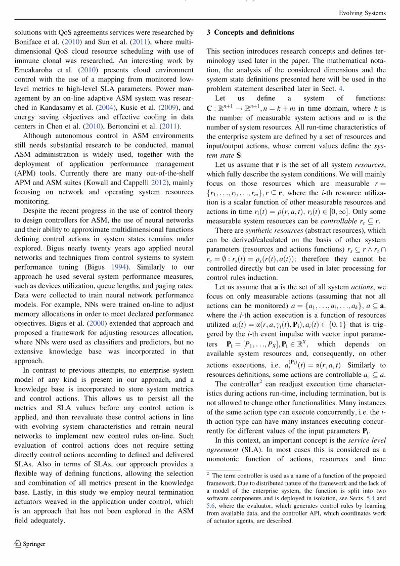
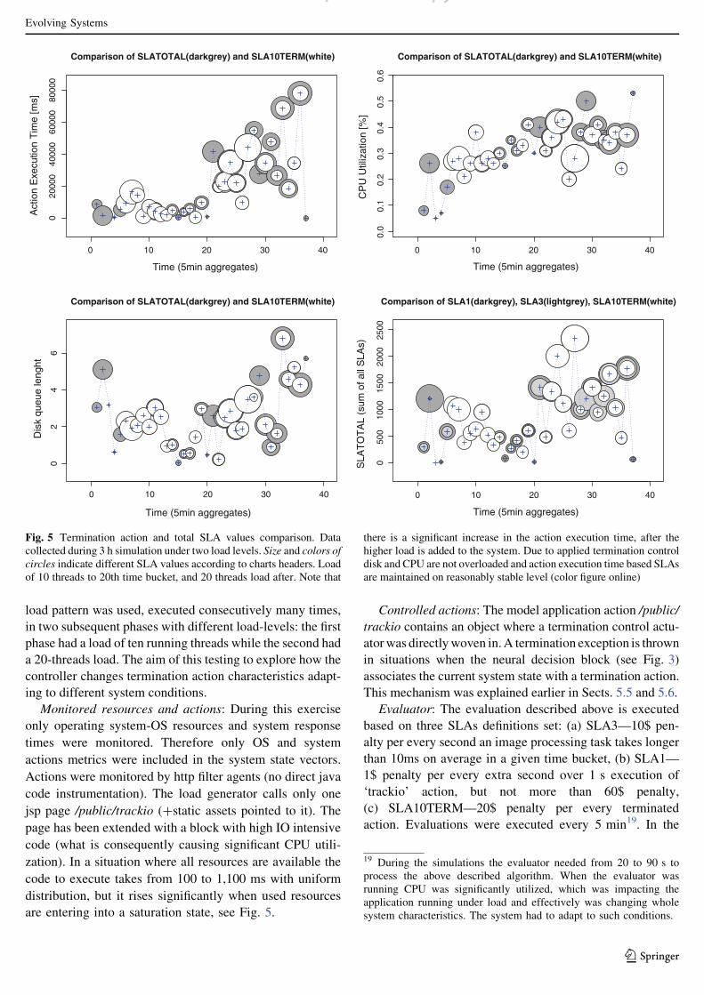
Fig. 5 Termination action and total SLA values comparison. Data

collected during 3 h simulation under two load levels. Size and colors of

circles indicate different SLA values according to charts headers. Load

of 10 threads to 20th time bucket, and 20 threads load after. Note that

there is a significant increase in the action execution time, after the

higher load is added to the system. Due to applied termination control

disk and CPU are not overloaded and action execution time based SLAs

are maintained on reasonably stable level (color figure online)

19 During the simulations the evaluator needed from 20 to 90 s to

process the above described algorithm. When the evaluator was

running CPU was significantly utilized, which was impacting the

application running under load and effectively was changing whole

system characteristics. The system had to adapt to such conditions.

Evolving Systems

123

p py

simulation, a 1 h sliding window was used to access system

states repository data. These SLAs definitions were used in

all simulations presented in the paper. The definitions used

are nontrivial in order to demonstrate the adaptive control

behavior in the background of nonlinear system perfor-

mance requirements (where nonlinear factors are present in

dependencies between the system execution and charac-

teristics of services performance perceived by clients).

6.2 Simulations and results

This section describes our experiments and discusses

results confirming the adaptive nature of the controller

using data from three scenarios. In these simulations we

focused on runs of medium length, i.e. up to 4 h for a

single simulation run.

6.2.1 Single load testing

In this scenario, we investigate the controlled system

dynamics using a single load test simulation, with two

subsequent load levels.

System states were generated for three dimensions being

evaluated (CPUUSER, DISKQUEUE, and MEMORY).

Figure 5 shows a comparison between SLAs values (cir-

cles), action execution times and main resources (CPU

utilization and disk queue length) as a function of time (in

5 min time buckets—aggregates). All metrics were recor-

ded during 3 h simulation under two load levels. The main

objective was to optimize the SLAs; thus, the controller

tried to keep the TOTALSLA on minimal level, balancing

termination penalties (SLA10TERM), long running actions

(SLA1), and potentially massive static assets execution

penalties in cases of high resources consumption (SLA3).

The result not only provides a reasonable constant level

of total SLAs but also maintains low level of resources

utilization. Actions that could lead to full resources satu-

ration are normally avoided, as in these cases execution

times raise exponentially effectively causing higher SLA

penalties (Hellerstein et al. 2004). Simulations showed that

the neural controller approach can adapt and optimize the

operation of a system under load conditions based on

objective functions defined as SLAs.

The two load patterns used during the run are best vis-

ible on the top left chart on Fig. 5, when action execution

time rises significantly after adding twice the load to the

system. At the beginning of the run no control was applied

(SLA10TERM was low), because the evaluator had not

established any ‘‘good’’ and ‘‘bad’’ states for potential

termination control yet. Just after the 5th time bucket the

controller decides on the first termination actions (white

circles), which leads to lowering DISKQUEUE, SLA1 and

SLA3. It is worth noting the gradual decrease of

cumulative SLA value during the first phase. The trend was

broken after 20th bucket when more load was added to the

system.

Surprisingly the first time buckets of the second phase

show no termination action (no white circles)—that was

because the new conditions were so different that the

controller could not match the new system states with those

represented in the trained NNs. A new evaluation process

was needed to train the NNs and propagate the decision

block objects to the application in order to control the new

situation. Just after the controller begins terminating

actions, this causes massive growth of total SLA (mainly

penalties for termination), still maintaining reasonable low

resources consumption. Around the 30th time bucket the

controller (considering states of the recent past) changes

the strict operating mode, so significantly less termination

actions are applied. Consequently, more actions are called

and utilization of all resources increases. At the end of the

simulation the controller contains state definitions, which

allow the system to operate on a level of total 2,000$

penalty per time bucket, with quite high execution times

but reasonable resources utilized.

6.2.2 Load testing with different SLA penalties

This scenario demonstrates the adaptive nature of the

controller running in the background of different SLA

definitions. In order to test adaptability to different SLAs

variations, we chose to change the termination penalty but

keep the rest of SLAs unmodified (SLA1 and SLA3 men-

tioned above), effectively shaping the system performance

needs.

To simplify the discussion and the presentation of the

data collected, the Evaluator was setup to manage only two

resources dimensions through the actuator agents. Disk

queue length (DISKQUEUE) and CPU utilization (CPU)

were selected as best meeting the SLA definitions

dynamics. Thus, the Evaluator process and the agents

consider only those two resource values when applying the

control.

Four load tests were executed. Each load test takes

around 2 hours, and after each run a full system restart

takes place. Firstly, three identical load test were executed

for different termination penalty SLAs. For each run the

penalty for termination (SLA TERM) was modified starting

from 5, 10 to 20$ per termination. After that another load

test was run (no control—NT)—this time the Evaluator

process was switched off, so the actuator agents didn’t

receive a trained NN control module with rules. Effectively

no control can be applied, so every action requested is

executed, causing highest disk and CPU utilizations.

During each of the load runs the Evaluator was triggered

every 8 min, so there were at least 14 rules inductions

Evolving Systems

123

p py

processes. During the first 7 evaluations, the system was

tested with 10 and later with 20-threads load. The system

specification was as the one used in the first scenario, so the

same saturation effect took place—execution times of

actions are growing significantly after saturating a crucial

for the functionality performance resource. Variant B of

rules conflicts resolution was used, so the evaluator

removes states with lower cardinality in the conflicting

areas (see Sect. 5.4.3).

Let us review one of the evaluation runs to discuss

details of the rule induction process. Figure 4 shows rules

generated in the sixth evaluation run. The highest SLA

were associated with CPU states over 60 % and DISK-

QUEUE higher than 2 (see top chart in this figure). The

control system decided to terminate actions that were

executing under systems states that indicated higher disk

queue length. Note that in this figure, black color is used to

indicate training points for rules advising no termination,

while red symbols represent rules for termination.

Apparently high cardinality states—those with high

quantity of points measured in a given neighborhood—

appear in the area of empty disk queue, see the bottom

chart. Such states did not cause high SLAs even for sub-

stantially high CPU, compare the bottom with the top chart.

So the Evaluator found that in this case a termination

action is not appropriate (e.g. potential benefits are not

substantial, or penalties are too high), consequently no

termination was advised at these time points. It seems the

Evaluator established that disk utilization is the most sig-

nificant dimension for the current set of SLAs.

In order to illustrate the control behavior based on the

rules generated during the described evaluation process,

Fig. 4 presents with an ‘‘x’’ time points where effective

control decisions were taken by the neural controller. A red

‘‘x’’ indicates a terminated executions/actions, while a

black one non-terminated actions.

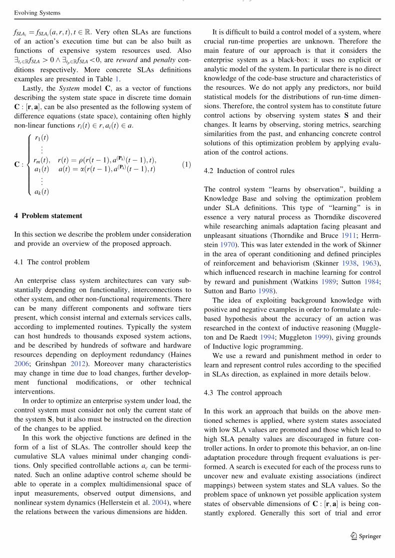
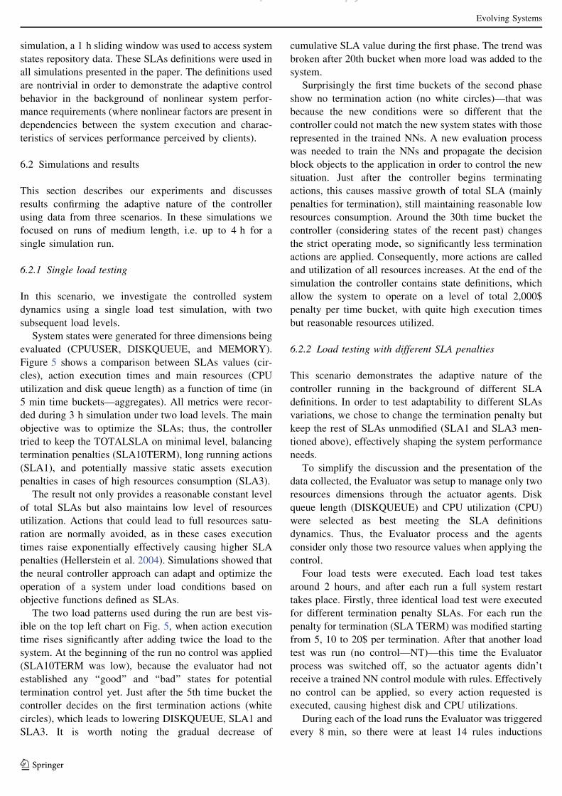
Figure 6 shows three snapshots of rule sets generated for

evaluation numbers 6, 9 and 13. This is analogous to the

charts presented in Fig. 4. Evaluation 6 was the last one

before the load applied on the system was doubled, from 10

to 20 threads. Note that evaluation 9 shows that a few more

rules promoting termination actions have appeared in the

0.0 0.2 0.4 0.6 0.8 1.0

05

1015

20

Evaluation #6, Comparison of SLATOTAL

CPU

DIS

KQ

UE

UE

Bad NN training setGood NN training setNo TerminationUse Termination

0.0 0.2 0.4 0.6 0.8 1.0

05

1015

20


CPU

DIS

KQ

UE

UE


0.0 0.2 0.4 0.6 0.8 1.0

05

1015

20


CPU

DIS

KQ

UE

UE


0.0 0.2 0.4 0.6 0.8 1.0

05

1015

20


CPU

DIS

KQ

UE

UE


0.0 0.2 0.4 0.6 0.8 1.0

05

1015

20


CPU

DIS

KQ

UE

UE


0.0 0.2 0.4 0.6 0.8 1.0

05

1015

20


CPU

DIS

KQ

UE

UE


Fig. 6 Training sets comparison generated by three different

subsequent evaluation processes. Data collected during 2 h simulation

under two load levels. Note the adaptive behavior between evalua-

tions after changing the load level (just before evaluation #9). Shapes

indicate the target NN in the decision block.Thus, circles represent

actions produced by the ‘‘good’’ neural network, while squares

decisions made by the ‘‘bad’’ neural network. Light red shapes

indicate supported termination control, whilst black color indicates no

control was applied. More detailed description can be found in Sect.

5.5 (color figure online)

Evolving Systems

123

p py

area of higher DISKQUEUE and CPU values. These are

quite important from SLA value perspective (see SLA-

TOTAL in the top row), but not frequently recorded (there

is a low cardinality—see the bottom row). Evaluation 13

demonstrates a much more mature behavior, where rules

have moved to capture higher values in the observed

dimensions. In this way, the controller actuators respond to

the changes in the enterprise system adaptively.

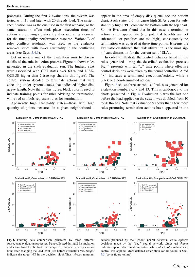
Figure 7 presents comparison of testbed dynamics dur-

ing four load runs, denoted as ‘‘05’’, ‘‘10’’, ‘‘20’’ and

‘‘NT’’, from four different perspectives, as discussed in the

text. The top two charts contain changes in the values of

the two main dimensions values using two minutes time

buckets. The bottom left chart presents the system states in

two dimensions illustrating the relationship between them.

The bottom right shows density of DISKQUEUE values

(number of data points) per each run. The curves are

plotted against the dimension value using LOESS

smoothing (Cleveland and Devlin 1988; Ripley 2012).

During 10-threads load, the control system operates at a

fairly stable level—both dimensions are stable for the

control runs. The situation changes at around the 30th time

bucket when a 20-threads load is applied to the system. The

utilizations raise for a few minutes, but then the controller

learns the new observed dimension values and adapts to the

new conditions lowering the utilizations by further

0

2

4

6

8

10

0 20 40 60TIME

DIS

KQ

UE

UE

SLATOTAL50010001500

RUN051020NT

Disk Queue Length in Time

0.2

0.4

0.6

0.8

0 20 40 60TIME

CP

USLATOTAL

50010001500

RUN051020NT

CPU utilization in Time

0

5

10

0.2 0.4 0.6 0.8

CPU

DIS

KQ

UE

UE

SLATOTAL50010001500

RUN051020NT

Disk Queue Length in CPU utilization

0.00

0.05

0.10

0.15

0.20

0 2 4 6 8 10

DISKQUEUE

dens

ity

RUN051020NT

Distribution of Disk Queue Length

Fig. 7 Comparison of main dimensions and total SLA values in four

test runs for three different termination penalties SLAs and a case of

no-control load (NT). All data were collected during 2 h simulations

under the same load patterns with two subsequent load levels. Circles

size indicates cumulative SLA values in each data bucket of presented

runs marked with different colors. In order to help interpret system

state changes the charts contain LOESS smoothed trends of adaptive

change of selected resources utilizations (confidence level interval is

set to default 0.95)

Evolving Systems

123

p py

terminations, especially DISKQUEUE which is primarily

used by the tested action functionality.

It is worth mentioning that the controller setup with the

‘‘cheapest’’ SLA termination penalty (run ‘‘05’’) tends to

use more termination actions, but the overall cost should

remain at a lower level than the SLA costs of running an

overloaded system. Apparently, when the penalty function

values are low the evaluation process tend to consider most

of control actions as ‘‘good’’, so the rules generation is

limited mainly by the size of the rule set (see Sect. 5.4.1)—

this generates imprecise control actions.

The reader may also notice that in the ‘‘10’’ and ‘‘20’’

runs the controller reacts to changes faster. During load

tests with non-controlled application (denoted by ‘‘NT’’),

after reaching a point of resources saturation—shortly after

the 20-threads load is introduced—trends are constantly

growing. This clearly shows that the system is overloaded

and not able to perform requested actions, which of course

does not happen when the controller is used.

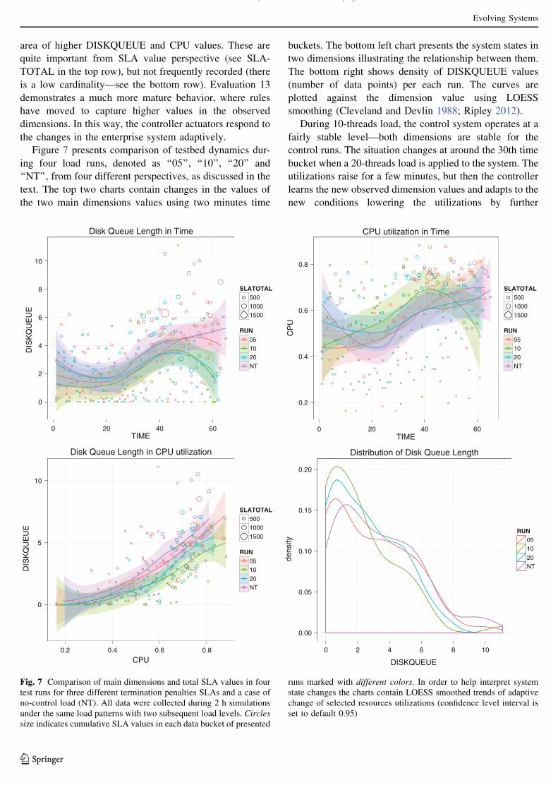
6.2.3 Load testing with different conflict resolution

strategies

This testing scenario concerns a set of load runs that

demonstrate the controller behavior using three different

strategies of resolving conflicts. These are Variants A–C

which were explained earlier in Sect. 5.4.3. The load pat-

terns, SLA definitions (penalty for termination is 10$), and

the rest of the testbed parameters remain the same as in

previous tests. Note that a slightly different set of dimen-

sions has been used, namely DISKQUEUE and CPUUSER.

In the tested scenarios, Variant A (the most strict strat-

egy) produces higher values for the SLAs and the response

to changes is slower than with other variants (promoting

states considered as part of ‘‘habits’’ or ‘‘trauma’’). This is

caused mainly by the fact that training sets are much

shorter, and simply not rich enough in terms of control

information. Situations where too many contradicting rules

appear in the same neighborhood of states are mainly

occurring at the start of the simulation run (i.e. a type of

cold start problem), or when the run-time process charac-

teristics change drastically. As a result the controller

appears less active, which is explained by the fact that a

short training set normally prevents the neural networks

from developing appropriate internal representations and

learn accurate control actions, and effectively there is less

to learn from the system responses after control application

(see details presented on Fig. 8).

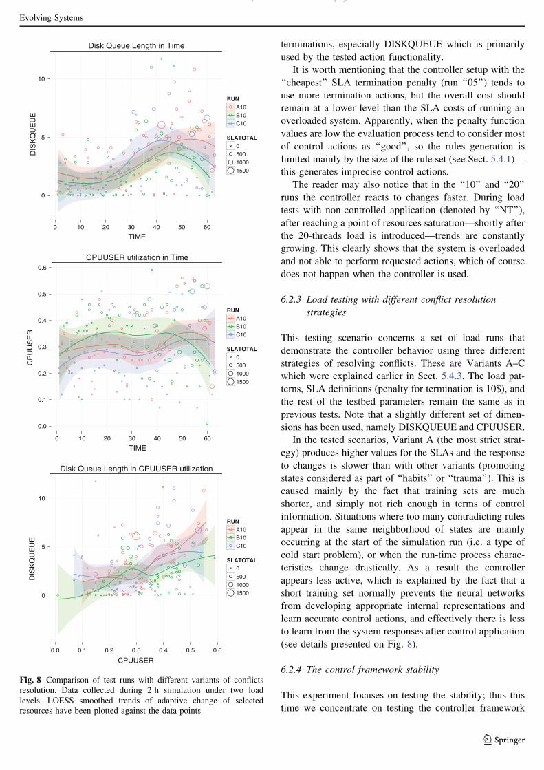
6.2.4 The control framework stability

This experiment focuses on testing the stability; thus this

time we concentrate on testing the controller framework

0

5

10

TIME

DIS

KQ

UE

UE

RUNA10B10C10

SLATOTAL05001000

1500


0.0

0.1

0.2

0.3

0.4

0.5

0.6

TIME

CP

UU

SE

R

RUNA10B10C10

SLATOTAL05001000

1500

CPUUSER utilization in Time

0

5

10

0 10 20 30 40 50 60

0 10 20 30 40 50 60

0.0 0.1 0.2 0.3 0.4 0.5 0.6

CPUUSER

DIS

KQ

UE

UE

RUNA10B10C10

SLATOTAL05001000

1500

Disk Queue Length in CPUUSER utilization

Fig. 8 Comparison of test runs with different variants of conflicts

resolution. Data collected during 2 h simulation under two load

levels. LOESS smoothed trends of adaptive change of selected

resources have been plotted against the data points

Evolving Systems

123

p py

under the same run-time conditions, using a technique

similar to bounded-input bounded-output (BIBO) method

(Hellerstein et al. 2004; Slotine et al. 1991; Astrom and

Wittenmark 2008).

We execute the load test many times using the same run-

time specification, i.e. the framework and application

parameters, incoming load level and pattern, conflicts res-

olution strategy (Variant B). To observe the trends the

load-test was executed longer than previously: for 4 h.

Figure 9 demonstrates data collected during the tests. The

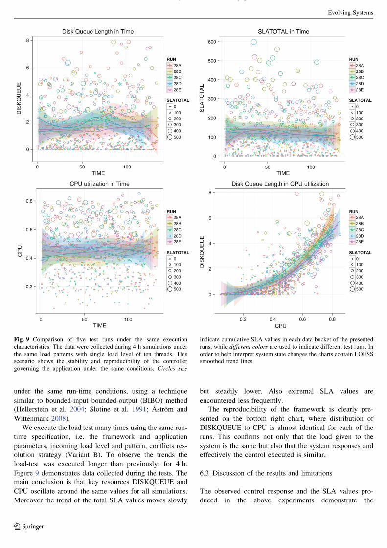
main conclusion is that key resources DISKQUEUE and

CPU oscillate around the same values for all simulations.

Moreover the trend of the total SLA values moves slowly

but steadily lower. Also extremal SLA values are

encountered less frequently.

The reproducibility of the framework is clearly pre-

sented on the bottom right chart, where distribution of

DISKQUEUE to CPU is almost identical for each of the

runs. This confirms not only that the load given to the

system is the same but also that the system responses and

effectively the control executed is similar.

6.3 Discussion of the results and limitations

The observed control response and the SLA values pro-

duced in the above experiments demonstrate the

0

2

4

6

8

0 50 100TIME

DIS

KQ

UE

UE

RUN28A28B28C28D28E

SLATOTAL0100200300400

500


0

100

200

300

400

500

600

0 50 100TIME

SLA

TO

TA

L

RUN28A28B28C28D28E

SLATOTAL0100200300400

500

SLATOTAL in Time

0.2

0.4

0.6

0.8

0 50 100TIME

CP

U

RUN28A28B28C28D28E

SLATOTAL0100200300400

500

CPU utilization in Time

0

2

4

6

8

0.2 0.4 0.6 0.8CPU

DIS

KQ

UE

UE

RUN28A28B28C28D28E

SLATOTAL0100200300400

500

Disk Queue Length in CPU utilization

Fig. 9 Comparison of five test runs under the same execution

characteristics. The data were collected during 4 h simulations under

the same load patterns with single load level of ten threads. This

scenario shows the stability and reproducibility of the controller

governing the application under the same conditions. Circles size

indicate cumulative SLA values in each data bucket of the presented

runs, while different colors are used to indicate different test runs. In

order to help interpret system state changes the charts contain LOESS

smoothed trend lines

Evolving Systems

123

p py

effectiveness of the controller design scheme and the

reproducibility of simulations. In Sect. 6.2.4 we showed

that the controller is stable under the same run-time con-

ditions. Moreover, similar adaptive behavior was observed

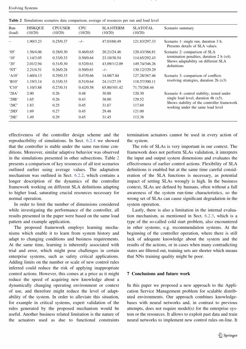
in the simulations presented in other subsections. Table 2

presents a comparison of key resources of all test scenarios

outlined earlier using average values. The adaptation

mechanism was outlined in Sect. 6.2.2, which contains a

longer description of the dynamics of the controller

framework working on different SLA definitions adapting

to higher load, saturating crucial resources necessary for

normal operation.

In order to limit the number of dimensions considered

while investigating the performance of the controller, all

results presented in the paper were based on the same load

pattern and example application.

The proposed framework employs learning mecha-

nisms which enable it to learn from system history and

adapt to changing conditions and business requirements.

At the same time, learning is inherently associated with

trial and error, which might pose challenges in certain

enterprise systems, such as safety critical applications.

Adding limits on the number or scale of new control rules

inferred could reduce the risk of applying inappropriate

control actions. However, this comes at a price as it might

reduce the speed of acquiring new knowledge about a

dynamically changing operating environment or context

of use, and therefore might reduce the level of adapt-

ability of the system. In order to alleviate this situation,

for example in critical systems, expert validation of the

rules generated by the proposed mechanism would be

useful. Another business related limitation is the nature of

the actuators used as due to functional constraints

termination actuators cannot be used in every action of

the system.

The role of SLAs is very important in our context. The

framework does not perform SLAs validation, it interprets

the input and output system dimensions and evaluates the

effectiveness of earlier control actions. Flexibility of SLA

definitions is enabled but at the same time careful consid-

eration of the SLA functions is necessary, as potential

impact of setting SLAs wrongly is high. In the business

context, SLAs are defined by humans, often without a full

awareness of the system run-time characteristics, so the

wrong set of SLAs can cause significant degradation in the

system operation.

Lastly, there is also a limitation in the internal evalua-

tion mechanism, as mentioned in Sect. 6.2.3, which is a

type of the so-called cold start problem, also encountered

in other systems, e.g. recommendation systems. At the

beginning of the controller operation, where there is still

lack of adequate knowledge about the system and the

results of the actions, or in cases when many contradicting

states are filtered out, training sets are shorter which means

that NNs training quality might be poor.

7 Conclusions and future work

In this paper we proposed a new approach to the Appli-

cation Service Management problem for scalable distrib-

uted environments. Our approach combines knowledge-

bases with neural networks and, in contrast to previous

attempts, does not require model(s) for the enterprise sys-

tem or the resources. It allows to exploit past data and train

neural networks to implement new control rules on-line. It

Table 2 Simulations scenarios data comparison; average of resources per run and load level

Run

(load)

DISKQUE

(10/20)

CPUUSER

(10/20)

CPU

(10/20)

SLA10TERM

(10/20)

SLATOTAL

(10/20)

Scenario summary

– 1.90/3.23 0.25/0.37 –/– 47.03/60.49 121.83/297.33 Scenario 1: single run, duration 3 h.

Presents details of SLA values.

‘05’ 1.56/4.06 0.28/0.30 0.46/0.65 20.21/24.46 120.43/366.81 Scenario 2: comparison of SLA

termination penalties, duration 2 h (x4).

Shows adaptability on different SLA

definitions

‘10’ 1.14/3.05 0.33/0.33 0.50/0.64 23.10/30.54 114.65/292.43

‘20’ 2.01/2.94 0.31/0.30 0.52/0.61 43.09/112.09 149.74/346.26

‘NT’ 2.21/4.51 0.26/0.28 0.50/0.61 –/– 130.12/329.29

‘A10’ 1.60/4.13 0.29/0.33 0.47/0.66 14.08/7.84 127.28/367.46 Scenario 3: comparison of conflicts

resolving strategies, duration 2h (x3)‘B10’ 1.19/3.14 0.33/0.33 0.51/0.64 24.11/27.19 118.57/300.11

‘C10’ 1.10/3.88 0.27/0.31 0.42/0.58 65.80/101.42 71.75/268.44

‘28A’ 2.00 0.26 0.48 30.88 120.30 Scenario 4: control stability, tested under

single load level, duration 4h (x5).

Shows stability of the controller framework

working under the same load level

‘28B’ 1.65 0.26 0.43 38.00 129.52

‘28C’ 1.83 0.25 0.45 31.67 117.69

‘28D’ 1.69 0.27 0.45 29.48 121.00

‘28E’ 1.49 0.29 0.45 31.45 113.38

Evolving Systems

123

p py

offers a flexible way of defining service level agreement

functions, allowing the selection and combination of met-

rics present in the knowledge base.

The applicability and effectiveness of the proposed

scheme was evaluated using a knowledge base with many

gigabytes of system run-time metrics. Empirical results

showed that neural networks-based controllers equipped

with a simple states evaluator are able to adapt to changing

run-time conditions based on SLA definitions. Due to the

nature of the knowledge based approach, larger data sets

would provide even stronger evidence of the controllers

performance. This will include extending the test-bed with

different applications and different run-time characteristics

to collect additional evidence on the effectiveness and

stability of our design in different contexts, e.g. resources

modification, actions microscheduling, caching services

tuning etc. This is indeed part of our future investigation,

together with the design and deployment of black and grey-

box controllers for more complicated cases, where more

actions with different run-time characteristics and new

types of actuators are present.

Acknowledgments This work was partially sponsored by Solid

Software Solutions (http://www.solidsoftware.pl/).

References

(2012a) Allmon, a generic system collecting and storing metrics used

for performance and availability monitoring. http://code.google.

com/p/allmon/

(2012b) DDD sample application, the project is a joint effort by Eric

Evans’ company domain language and the Swedish software

consulting company Citerus. http://dddsample.sourceforge.net/

Abdelzaher T, Lu C (2000) Modeling and performance control of

internet servers. In: Proceedings of the 39th IEEE conference on

decision and control, vol 3. IEEE, pp 2234–2239

Abdelzaher T, Shin K, Bhatti N (2002) Performance guarantees for

web server end-systems: a control-theoretical approach. IEEE

Trans Parallel Distrib Syst 13(1):80–96

Abdelzaher T, Stankovic J, Lu C, Zhang R, Lu Y (2003) Feedback

performance control in software services. IEEE Control Syst

23(3):74–90

Abeel T, Van de Peer Y, Saeys Y (2009) Java-ml: a machine learning

library. J Mach Learn Res 10:931–934

Abrahao B, Almeida V, Almeida J, Zhang A, Beyer D, Safai F (2006)

Self-adaptive sla-driven capacity management for internet ser-

vices. In: Network operations and management symposium,

2006. NOMS 2006. 10th IEEE/IFIP, IEEE, pp 557–568

Apache (2004) Version 2.0. The Apache Software Foundation:

Apache License, Version 20

Aston P, Fitzgerald C (2005) The grinder, a java load testing

framework. http://grinder.sourceforge.net/

Astrom KJ, Wittenmark B (2008) Adaptive control. Dover

Publications

Bertoncini M, Pernici B, Salomie I, Wesner S (2011) Games: green

active management of energy in it service centres. Information

systems evolution, pp 238–252

Bigus J (1994) Applying neural networks to computer system

performance tuning. In: 1994 IEEE international conference on

neural networks, 1994. IEEE world congress on computational

intelligence, vol 4. IEEE, pp 2442–2447

Bigus J, Hellerstein J, Jayram T, Squillante M (2000) Autotune: a

generic agent for automated performance tuning. Practical

application of intelligent agents and multi agent technology

Bodık P, Griffith R, Sutton C, Fox A, Jordan M, Patterson D (2009)

Statistical machine learning makes automatic control practical

for internet datacenters. In: Proceedings of the 2009 conference

on hot topics in cloud computing, HotCloud, vol 9

Boniface M, Nasser B, Papay J, Phillips S, Servin A, Yang X, Zlatev

Z, Gogouvitis S, Katsaros G, Konstanteli K, et al (2010)

Platform-as-a-service architecture for real-time quality of service

management in clouds. In: 2010 Fifth international conference

on internet and web applications and services (ICIW). IEEE,

pp 155–160

Brown B, Chui M, Manyika J (2011) Are you ready for the era of big

data? McKinsey Global Institute

Buyya R, Yeo C, Venugopal S (2008) Market-oriented cloud

computing: vision, hype, and reality for delivering it services

as computing utilities. In: 10th IEEE international conference on

high performance computing and communications, 2008.

HPCC’08. IEEE, pp 5–13

Buyya R, Yeo C, Venugopal S, Broberg J, Brandic I (2009) Cloud

computing and emerging it platforms: vision, hype, and reality

for delivering computing as the 5th utility. Future Gen Comput

Syst 25(6):599–616

Chen Y, Gmach D, Hyser C, Wang Z, Bash C, Hoover C, Singhal S

(2010) Integrated management of application performance, power

and cooling in data centers. In: 2010 IEEE network operations and

management symposium (NOMS). IEEE, pp 615–622

Cleveland W, Devlin S (1988) Locally weighted regression: an

approach to regression analysis by local fitting. J Am Stat Assoc

83(403):596–610

Coward D, Yoshida Y (2003) Java servlet specification version 2.3.

Sun Microsystems

Emeakaroha V, Brandic I, Maurer M, Dustdar S (2010) Low level

metrics to high level slas-lom2his framework: bridging the gap

between monitored metrics and sla parameters in cloud envi-

ronments. In: 2010 international conference on high performance

computing and simulation (HPCS). IEEE, pp 48–54

Evans E (2004) Domain-driven design: tackling complexity in the

heart of software. Addison-Wesley Professional

Fodor I (2002) A survey of dimension reduction techniques, vol 9.

Center for Applied Scientific Computing, Lawrence Livermore

National Laboratory, pp 1–18

Grinshpan L (2012) Solving enterprise applications performance

puzzles: queuing models to the rescue. Wiley Online Library

Guyon I, Elisseeff A (2003) An introduction to variable and feature

selection. J Mach Learn Res 3:1157–1182

Haines S (2006) Pro Java EE 5 performance management and

optimization. Apress

Hellerstein J (2004) Challenges in control engineering of computing

systems. In: American Control Conference, 2004. Proceedings of

the 2004, IEEE 3:1970–1979

Hellerstein J, Parekh S, Diao Y, Tilbury D (2004) Feedback control of

computing systems. Wiley–IEEE Press

Herrnstein R (1970) On the law of effect. J Exp Anal Behav 13(2):243

Kandasamy N, Abdelwahed S, Hayes J (2004) Self-optimization in

computer systems via on-line control: application to power

management. In: Proceedings of the international conference on

autonomic computing, 2004. IEEE, pp 54–61

Kiczales G, Lamping J, Mendhekar A, Maeda C, Lopes C, Loingtier

J, Irwin J (1997) Aspect-oriented programming. ECOOP’97

object-oriented programming, pp 220–242

Kowall J, Cappelli W (2012) Magic quadrant for application

performance monitoring. Gartner Research ID:G00232180

Evolving Systems

123

p py

Kusic D, Kephart J, Hanson J, Kandasamy N, Jiang G (2009) Power

and performance management of virtualized computing envi-

ronments via lookahead control. Cluster Comput 12(1):1–15

Laddad R (2009) Aspectj in action: enterprise AOP with spring

applications. Manning Publications Co.

Lu Y, Abdelzaher T, Lu C, Tao G (2002) An adaptive control

framework for qos guarantees and its application to differenti-

ated caching. In: Tenth IEEE international workshop on quality

of service, 2002. IEEE, pp 23–32

Lu Y, Abdelzaher T, Lu C, Sha L, Liu X (2003) Feedback control

with queueing-theoretic prediction for relative delay guarantees

in web servers. In: Proceedings of the 9th IEEE real-time and

embedded technology and applications symposium, 2003. IEEE,

pp 208–217

Muggleton S (1999) Inductive logic programming: issues, results and

the challenge of learning language in logic. Artif Intell

114(1):283–296

Muggleton S, De Raedt L (1994) Inductive logic programming:

theory and methods. J Logic Program 19:629–679

Parekh S, Gandhi N, Hellerstein J, Tilbury D, Jayram T, Bigus J

(2002) Using control theory to achieve service level objectives in

performance management. Real Time Syst 23(1):127–141

Park L, Baek J, Woon-Ki Hong J (2001) Management of service level

agreements for multimedia internet service using a utility model.

IEEE Commun Mag 39(5):100–106

Patel P, Ranabahu A, Sheth A (2009) Service level agreement in

cloud computing. In: Cloud workshops at OOPSLA

Powley W, Martin P, Ogeer N, Tian W (2005) Autonomic buffer pool

configuration in postgresql. In: 2005 IEEE international confer-

ence on systems, man and cybernetics, vol 1. IEEE, pp 53–58

Ripley BD (2012) Lowees scatter plot smoothing, r statistical data

analysis, r documentation. http://stat.ethz.ch/R-manual/R-

patched/library/stats/html/lowess.html

Saeys Y, Abeel T, Van de Peer Y (2008) Robust feature selection

using ensemble feature selection techniques. Machine learning

and knowledge discovery in databases, pp 313–325

Skinner B (1938) The behavior of organisms: an experimental

analysis

Skinner B (1963) Operant behavior. Am Psychol 18(8):503

Slotine JJE, Li W et al (1991) Applied nonlinear control, vol 1.

Prentice Hall, New Jersey

Stantchev V, Schropfer C (2009) Negotiating and enforcing qos and

slas in grid and cloud computing. Advances in grid and pervasive

computing, pp 25–35

Sun D, Chang G, Li F, Wang C, Wang X (2011) Optimizing multi-

dimensional qos cloud resource scheduling by immune clonal

with preference. Acta Electron Sin 8:018

Sutton R (1984) Temporal credit assignment in reinforcement

learning. PhD thesis

Sutton R, Barto A (1998) Reinforcement learning: an introduction,

vol 1. Cambridge University Press, Cambridge

Thorndike E, Bruce D (1911) Animal intelligence: experimental

studies. Transaction Pub

Vaquero L, Rodero-Merino L, Caceres J, Lindner M (2008) A break

in the clouds: towards a cloud definition. ACM SIGCOMM

Comput Commun Rev 39(1):50–55

Wang Z, Chen Y, Gmach D, Singhal S, Watson B, Rivera W, Zhu X,

Hyser C (2009) Appraise: application-level performance man-

agement in virtualized server environments. IEEE Trans Netw

Serv Manag 6(4):240–254

Watkins C (1989) Learning from delayed rewards. PhD thesis, King’s

College, Cambridge

Welsh M, Culler D (2002) Overload management as a fundamental

service design primitive. In: Proceedings of the 10th workshop

on ACM SIGOPS European workshop. ACM, pp 63–69

Welsh M, Culler D (2003) Adaptive overload control for busy internet

servers. In: Proceedings of the 4th USENIX conference on

internet technologies and systems, vol 2

Xiong P, Wang Z, Jung G, Pu C (2010) Study on performance

management and application behavior in virtualized environ-

ment. In: Network operations and management symposium

(NOMS), 2010 IEEE. IEEE, pp 841–844

Zhang A, Santos P, Beyer D, Tang H (2002a) Optimal server resource

allocation using an open queueing network model of response

time. HP laboratories Technical Report, HPL2002301

Zhang R, Lu C, Abdelzaher T, Stankovic J (2002b) Controlware: a

middleware architecture for feedback control of software

performance. In: Proceedings of the 22nd international confer-

ence on distributed computing systems, 2002. IEEE, pp 301–310

Evolving Systems

123

p py

neural adaptive control in application service …gmagoulas/nn-control-in-asm_evos-bb.pdf · neural...

Documents