neural networks - dlrl summer school · neural networks 2 • what we’ll cover ‣ types of...
TRANSCRIPT

Neural NetworksHugo Larochelle ( @hugo_larochelle )Google Brain

NEURAL NETWORKS 2
• What we’ll cover‣ types of learning problems
- definitions of popular learning problems- how to define an architecture for a learning problem
‣ unintuitive properties of neural networks- adversarial examples- optimization landscape of neural networks
...
Feedforward neural network
Hugo Larochelle
Departement d’informatiqueUniversite de Sherbrooke
September 6, 2012
Abstract
Math for my slides “Feedforward neural network”.
• a(x) = b+P
i wixi = b+w>x
• h(x) = g(a(x)) = g(b+P
i wixi)
• x1 xd
• w
• {
• g(·) b
• h(x) = g(a(x))
• a(x) = b(1) +W(1)x⇣a(x)i = b(1)i
Pj W
(1)i,j xj
⌘
• o(x) = g(out)(b(2) +w(2)>x)
1
...
Feedforward neural network
Hugo Larochelle
Departement d’informatiqueUniversite de Sherbrooke
September 6, 2012
Abstract
Math for my slides “Feedforward neural network”.
• a(x) = b+P
i wixi = b+w>x
• h(x) = g(a(x)) = g(b+P
i wixi)
• x1 xd b w1 wd
• w
• {
• g(a) = a
• g(a) = sigm(a) = 11+exp(�a)
• g(a) = tanh(a) = exp(a)�exp(�a)exp(a)+exp(�a) = exp(2a)�1
exp(2a)+1
• g(a) = max(0, a)
• g(a) = reclin(a) = max(0, a)
• g(·) b
• W (1)i,j b(1)i xj h(x)i
• h(x) = g(a(x))
• a(x) = b(1) +W(1)x⇣a(x)i = b(1)i
Pj W
(1)i,j xj
⌘
• o(x) = g(out)(b(2) +w(2)>x)
1
1
1
...... 1
......
...
Feedforward neural network
Hugo Larochelle
Departement d’informatiqueUniversite de Sherbrooke
September 13, 2012
Abstract
Math for my slides “Feedforward neural network”.
• f(x)
• l(f(x(t);✓), y(t))
• r✓l(f(x(t);✓), y(t))
• ⌦(✓)
• r✓⌦(✓)
• f(x)c = p(y = c|x)
• x(t) y(t)
• l(f(x), y) = �P
c 1(y=c) log f(x)c = � log f(x)y =
•
@
f(x)c� log f(x)y =
�1(y=c)
f(x)y
rf(x) � log f(x)y =�1
f(x)y[1(y=0), . . . , 1(y=C�1)]
>
=�e(c)
f(x)y
1
x

Neural NetworksTypes of learning problems
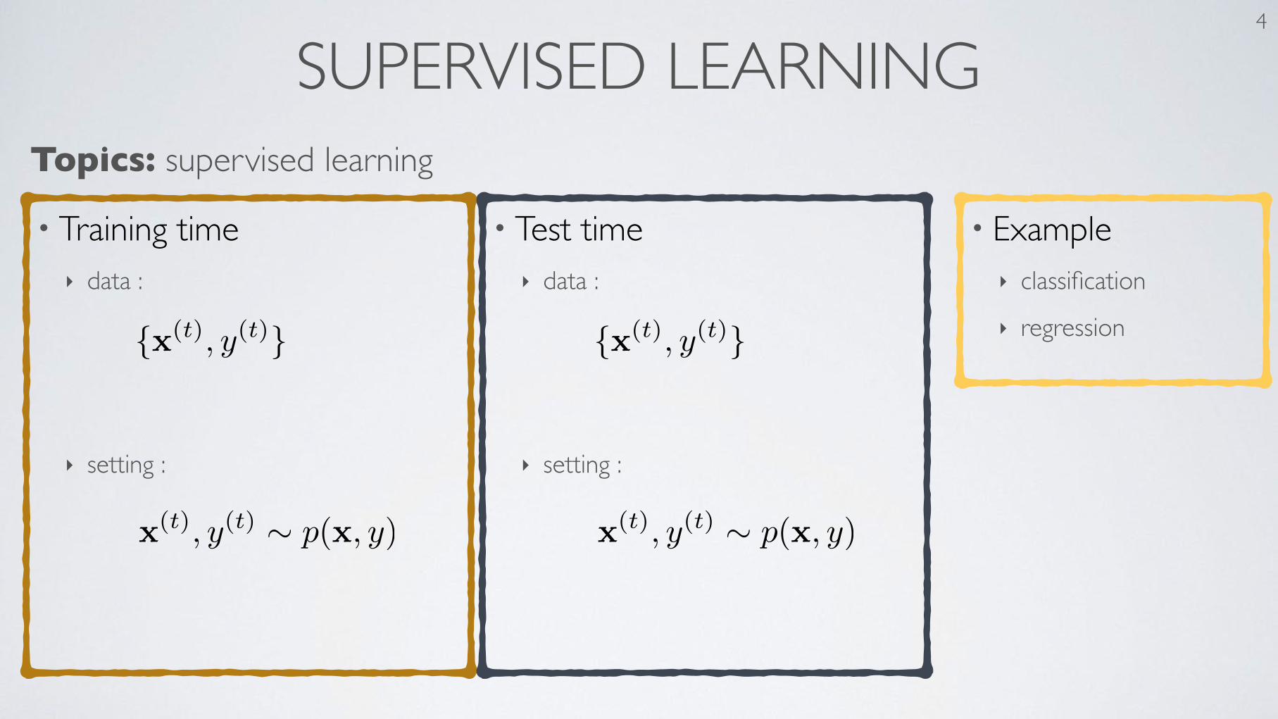
SUPERVISED LEARNING 4
Topics: supervised learning
• Training time‣ data :
‣ setting :
• Test time‣ data :
‣ setting :
{x(t), y(t)} {x(t), y(t)}
• Example‣ classification
‣ regression
x(t), y(t) ⇠ p(x, y) x(t), y(t) ⇠ p(x, y)

UNSUPERVISED LEARNING 5
Topics: unsupervised learning
• Training time‣ data :
‣ setting :
• Test time‣ data :
‣ setting :
{x(t)}{x(t)}
x(t) ⇠ p(x) x(t) ⇠ p(x)
• Example‣ distribution estimation
‣ dimensionality reduction

SEMI-SUPERVISED LEARNING 6
Topics: semi-supervised learning
• Training time‣ data :
‣ setting :
• Test time‣ data :
‣ setting :
{x(t), y(t)} {x(t), y(t)}{x(t)}
x(t) ⇠ p(x)
x(t), y(t) ⇠ p(x, y) x(t), y(t) ⇠ p(x, y)

MULTITASK LEARNING 7
Topics: multitask learning
• Training time‣ data :
‣ setting :
• Test time‣ data :
‣ setting :
{x(t), y(t)1 , . . . , y(t)M } {x(t), y(t)1 , . . . , y(t)M }
x(t), y(t)1 , . . . , y(t)M ⇠p(x, y1, . . . , yM )
x(t), y(t)1 , . . . , y(t)M ⇠p(x, y1, . . . , yM )
• Example‣ object recognition in
images with multiple objects

MULTITASK LEARNING 8
Topics: multitask learning
...
Feedforward neural network
Hugo Larochelle
Departement d’informatiqueUniversite de Sherbrooke
September 6, 2012
Abstract
Math for my slides “Feedforward neural network”.
• a(x) = b+P
i wixi = b+w>x
• h(x) = g(a(x)) = g(b+P
i wixi)
• x1 xd
• w
• {
• g(·) b
• h(x) = g(a(x))
• a(x) = b(1) +W(1)x⇣a(x)i = b(1)i
Pj W
(1)i,j xj
⌘
• o(x) = g(out)(b(2) +w(2)>x)
1
...
Feedforward neural network
Hugo Larochelle
Departement d’informatiqueUniversite de Sherbrooke
September 6, 2012
Abstract
Math for my slides “Feedforward neural network”.
• a(x) = b+P
i wixi = b+w>x
• h(x) = g(a(x)) = g(b+P
i wixi)
• x1 xd b w1 wd
• w
• {
• g(a) = a
• g(a) = sigm(a) = 11+exp(�a)
• g(a) = tanh(a) = exp(a)�exp(�a)exp(a)+exp(�a) = exp(2a)�1
exp(2a)+1
• g(a) = max(0, a)
• g(a) = reclin(a) = max(0, a)
• g(·) b
• W (1)i,j b(1)i xj h(x)i
• h(x) = g(a(x))
• a(x) = b(1) +W(1)x⇣a(x)i = b(1)i
Pj W
(1)i,j xj
⌘
• o(x) = g(out)(b(2) +w(2)>x)
1
......
......
...
• p(y = c|x)
• o(a) = softmax(a) =h
exp(a1)Pc exp(ac)
. . . exp(aC)Pc exp(ac)
i>
• f(x)
• h(1)(x) h(2)(x) W(1) W(2) W(3) b(1) b(2) b(3)
• a(k)(x) = b(k) +W(k)h(k�1)x (h(0)(x) = x)
• h(k)(x) = g(a(k)(x))
• h(L+1)(x) = o(a(L+1)(x)) = f(x)
2
• p(y = c|x)
• o(a) = softmax(a) =h
exp(a1)Pc exp(ac)
. . . exp(aC)Pc exp(ac)
i>
• f(x)
• h(1)(x) h(2)(x) W(1) W(2) W(3) b(1) b(2) b(3)
• a(k)(x) = b(k) +W(k)h(k�1)x (h(0)(x) = x)
• h(k)(x) = g(a(k)(x))
• h(L+1)(x) = o(a(L+1)(x)) = f(x)
2
• p(y = c|x)
• o(a) = softmax(a) =h
exp(a1)Pc exp(ac)
. . . exp(aC)Pc exp(ac)
i>
• f(x)
• h(1)(x) h(2)(x) W(1) W(2) W(3) b(1) b(2) b(3)
• a(k)(x) = b(k) +W(k)h(k�1)x (h(0)(x) = x)
• h(k)(x) = g(a(k)(x))
• h(L+1)(x) = o(a(L+1)(x)) = f(x)
2
• p(y = c|x)
• o(a) = softmax(a) =h
exp(a1)Pc exp(ac)
. . . exp(aC)Pc exp(ac)
i>
• f(x)
• h(1)(x) h(2)(x) W(1) W(2) W(3) b(1) b(2) b(3)
• a(k)(x) = b(k) +W(k)h(k�1)x (h(0)(x) = x)
• h(k)(x) = g(a(k)(x))
• h(L+1)(x) = o(a(L+1)(x)) = f(x)
2
y

MULTITASK LEARNING 8
Topics: multitask learning
...
Feedforward neural network
Hugo Larochelle
Departement d’informatiqueUniversite de Sherbrooke
September 6, 2012
Abstract
Math for my slides “Feedforward neural network”.
• a(x) = b+P
i wixi = b+w>x
• h(x) = g(a(x)) = g(b+P
i wixi)
• x1 xd
• w
• {
• g(·) b
• h(x) = g(a(x))
• a(x) = b(1) +W(1)x⇣a(x)i = b(1)i
Pj W
(1)i,j xj
⌘
• o(x) = g(out)(b(2) +w(2)>x)
1
Feedforward neural network
Hugo Larochelle
Departement d’informatiqueUniversite de Sherbrooke
September 6, 2012
Abstract
Math for my slides “Feedforward neural network”.
• a(x) = b+P
i wixi = b+w>x
• h(x) = g(a(x)) = g(b+P
i wixi)
• x1 xd
• w
• {
• g(·) b
• h(x) = g(a(x))
• a(x) = b(1) +W(1)x⇣a(x)i = b(1)i
Pj W
(1)i,j xj
⌘
• o(x) = g(out)(b(2) +w(2)>x)
1
...
Feedforward neural network
Hugo Larochelle
Departement d’informatiqueUniversite de Sherbrooke
September 6, 2012
Abstract
Math for my slides “Feedforward neural network”.
• a(x) = b+P
i wixi = b+w>x
• h(x) = g(a(x)) = g(b+P
i wixi)
• x1 xd b w1 wd
• w
• {
• g(a) = a
• g(a) = sigm(a) = 11+exp(�a)
• g(a) = tanh(a) = exp(a)�exp(�a)exp(a)+exp(�a) = exp(2a)�1
exp(2a)+1
• g(a) = max(0, a)
• g(a) = reclin(a) = max(0, a)
• g(·) b
• W (1)i,j b(1)i xj h(x)i
• h(x) = g(a(x))
• a(x) = b(1) +W(1)x⇣a(x)i = b(1)i
Pj W
(1)i,j xj
⌘
• o(x) = g(out)(b(2) +w(2)>x)
1
......
......
...
• p(y = c|x)
• o(a) = softmax(a) =h
exp(a1)Pc exp(ac)
. . . exp(aC)Pc exp(ac)
i>
• f(x)
• h(1)(x) h(2)(x) W(1) W(2) W(3) b(1) b(2) b(3)
• a(k)(x) = b(k) +W(k)h(k�1)x (h(0)(x) = x)
• h(k)(x) = g(a(k)(x))
• h(L+1)(x) = o(a(L+1)(x)) = f(x)
2
• p(y = c|x)
• o(a) = softmax(a) =h
exp(a1)Pc exp(ac)
. . . exp(aC)Pc exp(ac)
i>
• f(x)
• h(1)(x) h(2)(x) W(1) W(2) W(3) b(1) b(2) b(3)
• a(k)(x) = b(k) +W(k)h(k�1)x (h(0)(x) = x)
• h(k)(x) = g(a(k)(x))
• h(L+1)(x) = o(a(L+1)(x)) = f(x)
2
• p(y = c|x)
• o(a) = softmax(a) =h
exp(a1)Pc exp(ac)
. . . exp(aC)Pc exp(ac)
i>
• f(x)
• h(1)(x) h(2)(x) W(1) W(2) W(3) b(1) b(2) b(3)
• a(k)(x) = b(k) +W(k)h(k�1)x (h(0)(x) = x)
• h(k)(x) = g(a(k)(x))
• h(L+1)(x) = o(a(L+1)(x)) = f(x)
2
• p(y = c|x)
• o(a) = softmax(a) =h
exp(a1)Pc exp(ac)
. . . exp(aC)Pc exp(ac)
i>
• f(x)
• h(1)(x) h(2)(x) W(1) W(2) W(3) b(1) b(2) b(3)
• a(k)(x) = b(k) +W(k)h(k�1)x (h(0)(x) = x)
• h(k)(x) = g(a(k)(x))
• h(L+1)(x) = o(a(L+1)(x)) = f(x)
2
y......y3y1 2
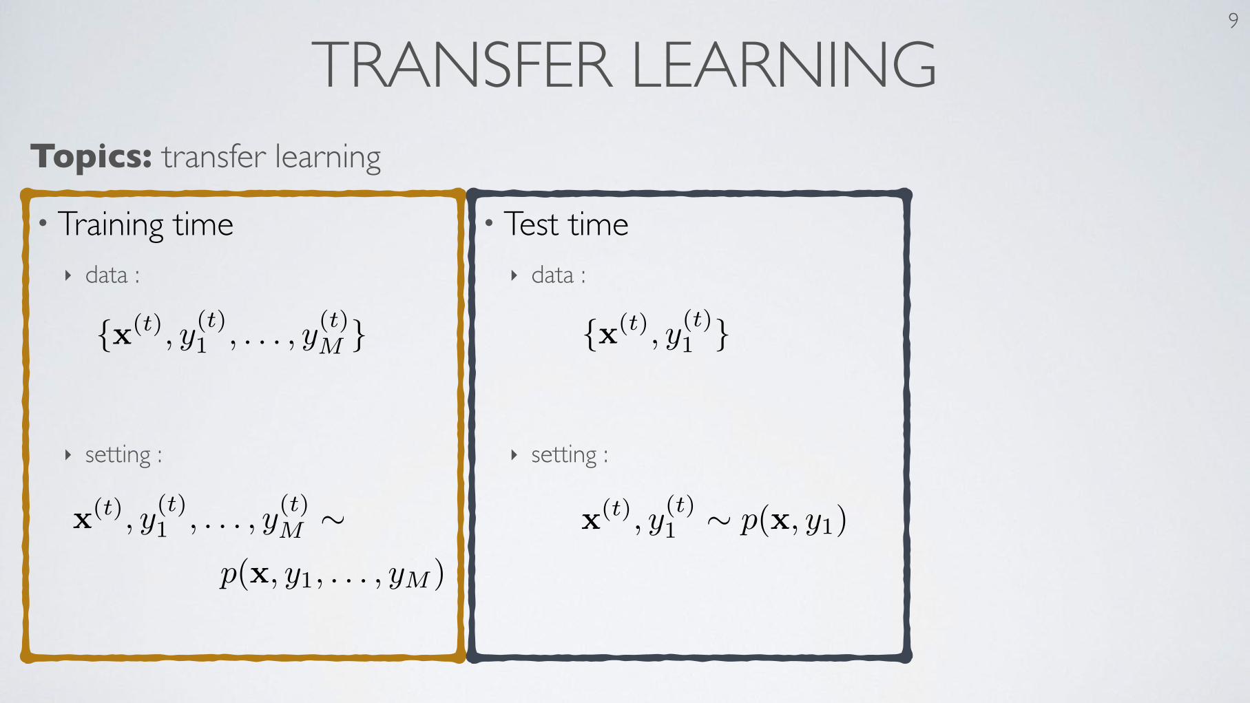
TRANSFER LEARNING 9
Topics: transfer learning
• Training time‣ data :
‣ setting :
• Test time‣ data :
‣ setting :
{x(t), y(t)1 , . . . , y(t)M }
x(t), y(t)1 , . . . , y(t)M ⇠p(x, y1, . . . , yM )
{x(t), y(t)1 }
x(t), y(t)1 ⇠ p(x, y1)

STRUCTURED OUTPUT PREDICTION 10
Topics: structured output prediction
• Training time‣ data :
‣ setting :
• Test time‣ data :
‣ setting :
• Example‣ image caption
generation
‣ machine translation
x(t),y(t) ⇠ p(x,y) x(t),y(t) ⇠ p(x,y)
{x(t),y(t)} {x(t),y(t)}of arbitrary structure
(vector, sequence, graph)

DOMAIN ADAPTATION 11
Topics: domain adaptation, covariate shift
• Training time‣ data :
‣ setting :
• Test time‣ data :
‣ setting :
{x(t), y(t)}
x(t) ⇠ p(x)
⇡ p(x)
• Example‣ classify sentiment in
reviews of different products
‣ training on synthetic data but testing on real data (sim2real)
y(t) ⇠ p(y|x(t))
{x(t), y(t)}
x(t) ⇠ q(x)
y(t) ⇠ p(y|x(t))
{x(t0)}
x(t) ⇠ q(x)

DOMAIN ADAPTATION 12
Topics: domain adaptation, covariate shift
x
Autoencoders
Hugo Larochelle
Departement d’informatique
Universite de Sherbrooke
October 17, 2012
Abstract
Math for my slides “Autoencoders”.
•
h(x) = g(a(x))
= sigm(b+Wx)
•
bx = o(ba(x))= sigm(c+W⇤h(x))
• f(x) ⌘ bx l(f(x)) = 12
Pk(bxk � xk)2 l(f(x)) = �
Pk (xk log(bxk) + (1� xk) log(1� bxk))
• rba(x(t))l(f(x(t))) = bx(t) � x(t)
a(x(t)) (= b+Wx(t)
h(x(t)) (= sigm(a(x(t)))
ba(x(t)) (= c+W>h(x(t))
bx(t) (= sigm(ba(x(t)))
rba(x(t))l(f(x(t))) (= bx(t) � x(t)
rcl(f(x(t))) (= rba(x(t))l(f(x
(t)))
rh(x(t))l(f(x(t))) (= W
⇣rba(x(t))l(f(x
(t)))⌘
ra(x(t))l(f(x(t))) (=
⇣rh(x(t))l(f(x
(t)))⌘� [. . . , h(x(t))j(1� h(x(t))j), . . . ]
rbl(f(x(t))) (= ra(x(t))l(f(x
(t)))
rWl(f(x(t))) (=⇣ra(x(t))l(f(x
(t)))⌘x(t)> + h(x(t))
⇣rba(x(t))l(f(x
(t)))⌘>
• W⇤ = W>
1
f(x)
W
V
b
c o(h(x))
w
d
• Domain-adversarial networks (Ganin et al. 2015) train hidden layer representation to be1.predictive of the target class2. indiscriminate of the domain
• Trained by stochastic gradient descent‣ for each random pair
1. update W,V,b,c in opposite direction of gradient
2. update w,d in direction of gradient
x(t), x(t0)
May also be used to promotefair and unbiased models …

ONE-SHOT LEARNING 13
Topics: one-shot learning
• Training time‣ data :
‣ setting :
• Test time‣ data :
‣ setting :
‣ side information :- a single labeled example from
each of the M new classes
{x(t), y(t)} {x(t), y(t)}
• Example‣ recognizing a person
based on a single picture of him/her
subject to y(t) 2 {1, . . . , C} y(t) 2 {C + 1, . . . , C +M}subject to
x(t), y(t) ⇠ p(x, y) x(t), y(t) ⇠ p(x, y)

ONE-SHOT LEARNING 14
Topics: one-shot learning
W
W
W
W
W
W
W
W
500
500
500
500
2000
Learning Similarity Metric
30
2000
1
2
3
4
30
1
2
3
4
y
X Xa b
ya bD[y ,y ]a b
Figure 1: After learning a non-linear transformation from imagesto 30-dimensional code vectors, the Euclidean distance betweencode vectors can be used to measure the similarity between im-ages.
Generalizing this idea to networks with multi-dimensional,real-valued outputs is difficult because the true mutual in-formation depends on the entropy of the output vectors andthis is hard to estimate efficiently for multi-dimensionaloutputs. Approximating the entropy by the log determi-nant of a multidimensional Gaussian works well for learn-ing linear transformations [7], because a linear transforma-tion cannot alter how Gaussian a distribution is. But it doesnot work well for learning non-linear transformations [21]because the optimization cheats by making the Gaussianapproximation to the entropy as bad as possible. The mu-tual information is the difference between the individual en-tropies and the joint entropy, so it can be made to appearvery large by learning individual output distributions thatresemble a hairball. When approximated by a Gaussian, alarge hairball has a large determinant but its true entropy isvery low because the density is concentrated into the hairsrather than filling the space.
The structure in an iid set of image pairs can be decom-posed into the structure in the whole iid set of individualimages, ignoring the pairings, plus the additional struc-ture in the way they are paired. If we focus on model-ing only the additional structure in the pairings, we canfinesse the problem of estimating the entropy of a multi-dimensional distribution. The additional structure can bemodeled by finding a non-linear transformation of each im-age into a low-dimensional code such that paired imageshave codes that are much more similar than images that arenot paired. Adopting a probabilistic approach, we can de-fine a probability distribution over all possible pairs of im-ages, by using the squared distances between theircodes, :
(2)
We can then learn the non-linear transformation by maxi-mizing the log probability of the pairs that actually occur inthe training set. The normalizing term in Eq. 2 is quadraticin the number of training cases rather than exponential inthe number of pixels or the number of code dimensions be-cause we are only attempting to model the structure in thepairings, not the structure in the individual images or themutual information between the code vectors.
The idea of using Eq. 2 to train a multilayer neural net-work was originally described in [9]. They showed thata network would extract a two-dimensional code that ex-plicitly represented the size and orientation of a face if itwas trained on pairs of face images that had the same sizeand orientation but were otherwise very different. Attemptsto extract more elaborate properties were less successfulpartly because of the difficulty of training multilayer neu-ral networks with many hidden layers, and partly becausethe amount of information in the pairings of images isless than bits per pair. This means that a very largenumber of pairs is required to train a large number of pa-rameters.
Chopra et.al. [3] have recently used a non-probabilistic ver-sion of the same approach to learn a similarity metric forfaces that assigns high similarity to very different images ofthe same person and low similarity to quite similar imagesof different people. They achieve the same effect as Eq.2 by using a carefully hand-crafted penalty function thatuses both positive (similar) and negative (dissimilar) exam-ples. They greatly reduce the number of parameters to belearned by using a convolutional multilayer neural networkand achieve impressive results on a face verification task.
We have recently discovered a very effective and entirelyunsupervised way of training a multi-layer, non-linear ”en-coder” network that transforms the input data vector intoa low-dimensional feature representation that cap-tures a lot of the structure in the input data [14]. This un-supervised algorithm can be used as a pretraining stage toinitialize the parameter vector that defines the mappingfrom input vectors to their low-dimensional representation.After the initial pretraining, the parameters can be fine-tuned by performing gradient descent in the Neighbour-hood Component Analysis (NCA) objective function intro-duced by [9]. The learning results in a non-linear trans-formation of the input space which has been optimized tomake KNN perform well in the low-dimensional featurespace. Using this nonlinear NCA algorithm to mapMNISTdigits into the 30-dimensional feature space, we achieve anerror rate of 1.08%. Support Vector Machines have a sig-nificantly higher error rate of 1.4% on the same version ofthe MNIST task [5].
In the next section we briefly review Neighborhood Com-ponents Analysis and generalize it to its nonlinear counter-part. In section 3, we show how one can efficiently per-
Siamese architecture(figure taken from Salakhutdinov
and Hinton, 2007)

ZERO-SHOT LEARNING 15
Topics: zero-shot learning, zero-data learning
• Training time‣ data :
‣ setting :
‣ side information :- description vector zc of each of
the C classes
• Test time‣ data :
‣ setting :
‣ side information :- description vector zc of each of
the new M classes
{x(t), y(t)} {x(t), y(t)}
• Example‣ recognizing an object
based on a worded description of it
subject to y(t) 2 {1, . . . , C} y(t) 2 {C + 1, . . . , C +M}subject to
x(t), y(t) ⇠ p(x, y) x(t), y(t) ⇠ p(x, y)

ZERO-SHOT LEARNING 16
Topics: zero-shot learning, zero-data learning
Predicting Deep Zero-Shot Convolutional Neural Networksusing Textual Descriptions
Jimmy Lei Ba Kevin Swersky Sanja Fidler Ruslan SalakhutdinovUniversity of Toronto
jimmy,kswersky,fidler,[email protected]
Abstract
One of the main challenges in Zero-Shot Learning of vi-
sual categories is gathering semantic attributes to accom-
pany images. Recent work has shown that learning from
textual descriptions, such as Wikipedia articles, avoids the
problem of having to explicitly define these attributes. We
present a new model that can classify unseen categories
from their textual description. Specifically, we use text fea-
tures to predict the output weights of both the convolutional
and the fully connected layers in a deep convolutional neu-
ral network (CNN). We take advantage of the architecture
of CNNs and learn features at different layers, rather than
just learning an embedding space for both modalities, as
is common with existing approaches. The proposed model
also allows us to automatically generate a list of pseudo-
attributes for each visual category consisting of words from
Wikipedia articles. We train our models end-to-end us-
ing the Caltech-UCSD bird and flower datasets and eval-
uate both ROC and Precision-Recall curves. Our empirical
results show that the proposed model significantly outper-
forms previous methods.
1. IntroductionThe recent success of the deep learning approaches to
object recognition is supported by the collection of largedatasets with millions of images and thousands of la-bels [3, 32]. Although the datasets continue to grow largerand are acquiring a broader set of categories, they are verytime consuming and expensive to collect. Furthermore, col-lecting detailed, fine-grained annotations, such as attributeor object part labels, is even more difficult for datasets ofsuch size.
On the other hand, there is a massive amount of textualdata available online. Online encyclopedias, such as En-glish Wikipedia, currently contain 4,856,149 articles, andrepresent a rich knowledge base for a diverse set of topics.Ideally, one would exploit this rich source of information in
CNNMLP
Classscore
Dotproduct
Wikipedia article
TF-IDF
Image
gf
The Cardinals or Cardinalidae are a family of passerine birds found in North and South AmericaThe South American cardinals in the genus…
fam
ily
north
genu
s
bird
s
sout
h
amer
ica
…
Cxk 1xk
1xC
Figure 1. A deep multi-modal neural network. The first modalitycorresponds to tf-idf features taken from a text corpus with a corre-sponding class, e.g., a Wikipedia article about a particular object.This is passed through a multi-layer perceptron (MLP) and pro-duces a set of linear output nodes f . The second modality takes inan image and feeds it into a convolutional neural network (CNN).The last layer of the CNN is then passed through a linear projec-tion to produce a set of image features g. The score of the class isproduced via f>g. In this setting, the text pipeline can be thoughtof as producing a set of classifier weights for the image pipeline.
order to train visual object models with minimal additionalannotation.
The concept of “Zero-Shot Learning” has been intro-duced in the literature [8, 9, 16, 20, 6] with the aim to im-prove the scalability of traditional object recognition sys-tems. The ability to classify images of an unseen class istransferred from the semantically or visually similar classesthat have already been learned by a visual classifier. Onepopular approach is to exploit shared knowledge betweenclasses in the form of attributes, such as stripes, four legs,
1
arX
iv:1
506.
0051
1v1
[cs.L
G]
1 Ju
n 20
15 Ba, Swersky, Fidler, Salakhutdinovarxiv 2015

DESIGNING NEW ARCHITECTURES 17
Topics: designing new architectures• Tackling a new learning problem often requires designing
an adapted neural architecture
• Approach 1: use our intuition for how a human would reason about the problem
• Approach 2: take an existing algorithm/procedure and turn it into a neural network

DESIGNING NEW ARCHITECTURES 18
Topics: designing new architectures• Many other examples‣ structured prediction by unrolling probabilistic inference in an MRF
‣ planning by unrolling the value iteration algorithm(Tamar et al., NIPS 2016)
‣ few-shot learning by unrolling gradient descent on small training setUnder review as a conference paper at ICLR 2017
Figure 1: Computational graph for the forward pass of the meta-learner. The dashed line dividesexamples from the training set Dtrain and test set Dtest. Each (Xi,Yi) is the ith batch from thetraining set whereas (X,Y) is all the elements from the test set. The dashed arrows indicate that wedo not back-propagate through that step when training the meta-learner. We refer to the learner asM , where M(X; ✓) is the output of learner M using parameters ✓ for inputs X. We also use rt asa shorthand for r✓t�1Lt.
to have training conditions match those of test time. During evaluation of the meta-learning, foreach dataset D = (Dtrain, Dtest) 2 Dmeta�test, a good meta-learner model will, given a series oflearner gradients and losses on the training set Dtrain, suggest a series of updates for the learnermodel that trains it towards good performance on the test set Dtest.
Thus to match test time, when considering each dataset D 2 Dmeta�train, the training objective weuse is the loss Ltest of the final learner model on D’s test set Dtest. While iterating over the examplesin D’s training set Dtrain, at each time step t the LSTM meta-learner receives (r✓t�1Lt,Lt) fromthe learner and proposes the new set of parameters ✓t. The process repeats for T steps, after whichthe learner and its final parameters are evaluated on the test set to produce the loss that is then usedto train the meta-learner. The training algorithm is described in Algorithm 1 and the correspondingcomputational graph is shown in Figure 1.
3.3.1 GRADIENT INDEPENDENCE ASSUMPTION
Notice that our formulation would imply that the losses Lt and gradients r✓t�1Lt of the learner aredependent on the parameters of the meta-learner. Gradients on the meta-learner’s parameters shouldnormally take this dependency into account. However, as discussed by Andrychowicz et al. (2016),this complicates the computation of the meta-learner’s gradients. Thus, following Andrychowiczet al. (2016), we make the simplifying assumption that these contributions to the gradients aren’timportant and can be ignored, which allows us to avoid taking second derivatives, a considerablyexpensive operation. We were still able to train the meta-learner effectively in spite of this simplify-ing assumption.
3.3.2 INITIALIZATION OF META-LEARNER LSTM
When training LSTMs, it is advised to initialize the LSTM with small random weights and to set theforget gate bias to a large value so that the forget gate is initialized to be close to 1, thus enablinggradient flow (Zaremba, 2015). In addition to the forget gate bias setting, we found that we neededto initialize the input gate bias to be small so that the input gate value (and thus the learning rate)used by the meta-learner LSTM starts out being small. With this combined initialization, the meta-learner starts close to normal gradient descent with a small learning rate, which helps initial stabilityof training.
4
Published as a conference paper at ICLR 2017
Figure 2: Computational graph for the forward pass of the meta-learner. The dashed line dividesexamples from the training set Dtrain and test set Dtest. Each (Xi,Yi) is the ith batch from thetraining set whereas (X,Y) is all the elements from the test set. The dashed arrows indicate that wedo not back-propagate through that step when training the meta-learner. We refer to the learner asM , where M(X; ✓) is the output of learner M using parameters ✓ for inputs X. We also use rt asa shorthand for r✓t�1Lt.
3.3.2 INITIALIZATION OF META-LEARNER LSTM
When training LSTMs, it is advised to initialize the LSTM with small random weights and to set theforget gate bias to a large value so that the forget gate is initialized to be close to 1, thus enablinggradient flow (Zaremba, 2015). In addition to the forget gate bias setting, we found that we neededto initialize the input gate bias to be small so that the input gate value (and thus the learning rate)used by the meta-learner LSTM starts out being small. With this combined initialization, the meta-learner starts close to normal gradient descent with a small learning rate, which helps initial stabilityof training.
3.4 BATCH NORMALIZATION
Batch Normalization (Ioffe & Szegedy, 2015) is a recently proposed method to stabilize and thusspeed up learning of deep neural networks by reducing internal covariate shift within the learner’shidden layers. This reduction is achieved by normalizing each layer’s pre-activation, by subtractingby the mean and dividing by the standard deviation. During training, the mean and standard devi-ation are estimated using the current batch being trained on, whereas during evaluation a runningaverage of both statistics calculated on the training set is used. We need to be careful with batchnormalization for the learner network in the meta-learning setting, because we do not want to collectmean and standard deviation statistics during meta-testing in a way that allows information to leakbetween different datasets (episodes), being considered. One easy way to prevent this issue is to notcollect statistics at all during the meta-testing phase, but just use our running averages from meta-training. This, however, has a bad impact on performance, because we have changed meta-trainingand meta-testing conditions, causing the meta-learner to learn a method of optimization that relieson batch statistics which it now does not have at meta-testing time. In order to keep the two phasesas similar as possible, we found that a better strategy was to collect statistics for each dataset D 2 Dduring Dmeta�test, but then erase the running statistics when we consider the next dataset. Thus,during meta-training, we use batch statistics for both the training and testing set whereas duringmeta-testing, we use batch statistics for the training set (and to compute our running averages) butthen use the running averages during testing. This does not cause any information to leak betweendifferent datasets, but also allows the meta-learner to be trained on conditions that are matched be-tween training and testing. Lastly, because we are doing very few training steps, we computed therunning averages so that higher preference is given to the later values.
5
Neural network
Learning algorithm
Ravi and Larochelle, ICLR 2017 _ _
_ _

Neural networksUnintuitive properties of neural networks

THEY CAN MAKE DUMB ERRORS 20
Topics: adversarial examples• Intriguing Properties of Neural Networks
Szegedy, Zaremba, Sutskever, Bruna, Erhan, Goodfellow, Fergus, ICLR 2014
(a) (b)
Figure 5: Adversarial examples generated for AlexNet [9].(Left) is a correctly predicted sample, (center) dif-ference between correct image, and image predicted incorrectly magnified by 10x (values shifted by 128 andclamped), (right) adversarial example. All images in the right column are predicted to be an “ostrich, Struthiocamelus”. Average distortion based on 64 examples is 0.006508. Plase refer to http://goo.gl/huaGPbfor full resolution images. The examples are strictly randomly chosen. There is not any postselection involved.
(a) (b)
Figure 6: Adversarial examples for QuocNet [10]. A binary car classifier was trained on top of the last layerfeatures without fine-tuning. The randomly chosen examples on the left are recognized correctly as cars, whilethe images in the middle are not recognized. The rightmost column is the magnified absolute value of thedifference between the two images.
the original training set all the time. We used weight decay, but no dropout for this network. Forcomparison, a network of this size gets to 1.6% errors when regularized by weight decay alone andcan be improved to around 1.3% by using carefully applied dropout. A subtle, but essential detailis that we only got improvements by generating adversarial examples for each layer outputs whichwere used to train all the layers above. The network was trained in an alternating fashion, maintain-ing and updating a pool of adversarial examples for each layer separately in addition to the originaltraining set. According to our initial observations, adversarial examples for the higher layers seemedto be significantly more useful than those on the input or lower layers. In our future work, we planto compare these effects in a systematic manner.
For space considerations, we just present results for a representative subset (see Table 1) of theMNIST experiments we performed. The results presented here are consistent with those on a largervariety of non-convolutional models. For MNIST, we do not have results for convolutional mod-els yet, but our first qualitative experiments with AlexNet gives us reason to believe that convolu-tional networks may behave similarly as well. Each of our models were trained with L-BFGS untilconvergence. The first three models are linear classifiers that work on the pixel level with variousweight decay parameters �. All our examples use quadratic weight decay on the connection weights:lossdecay = �
Pw2
i /k added to the total loss, where k is the number of units in the layer. Threeof our models are simple linear (softmax) classifier without hidden units (FC10(�)). One of them,FC10(1), is trained with extremely high � = 1 in order to test whether it is still possible to generateadversarial examples in this extreme setting as well.Two other models are a simple sigmoidal neuralnetwork with two hidden layers and a classifier. The last model, AE400-10, consists of a single layersparse autoencoder with sigmoid activations and 400 nodes with a Softmax classifier. This networkhas been trained until it got very high quality first layer filters and this layer was not fine-tuned. Thelast column measures the minimum average pixel level distortion necessary to reach 0% accuracy
on the training set. The distortion is measure byqP
(x0i�xi)2
n between the original x and distorted
6
Correctlyclassified
Badly classifiedDifference

THEY CAN MAKE DUMB ERRORS 21
Topics: adversarial examples• Humans have adversarial examples too
• However they don’t match those of neural networks

22
Topics: adversarial examples• Humans have adversarial examples too
• However they don’t match those of neural networks
THEY CAN MAKE DUMB ERRORS

THEY ARE STRANGELY NON-CONVEX 23
Topics: non-convexity, saddle points• Identifying and attacking the saddle point problem in high-dimensional non-convex optimization
Dauphin, Pascanu, Gulcehre, Cho, Ganguli, Bengio, NIPS 2014avg loss
θ
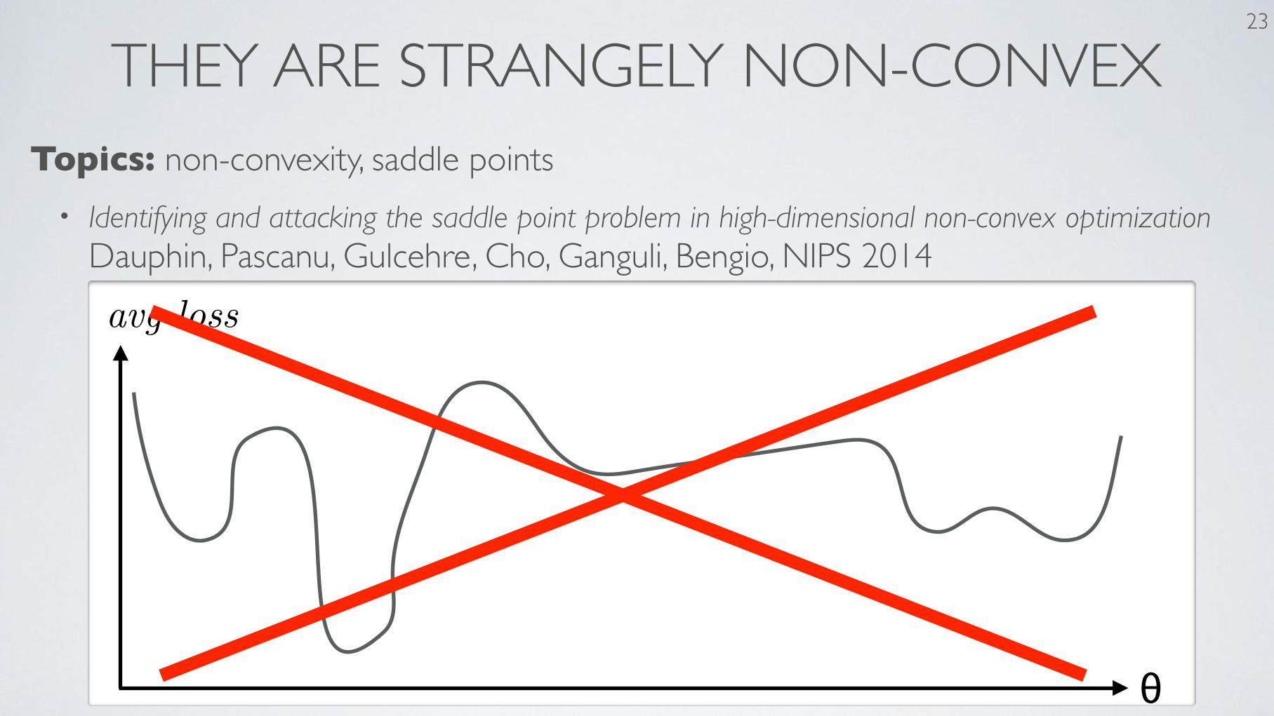
THEY ARE STRANGELY NON-CONVEX 23
Topics: non-convexity, saddle points• Identifying and attacking the saddle point problem in high-dimensional non-convex optimization
Dauphin, Pascanu, Gulcehre, Cho, Ganguli, Bengio, NIPS 2014avg loss
θ

THEY ARE STRANGELY NON-CONVEX 24
Topics: non-convexity, saddle points• Identifying and attacking the saddle point problem in high-dimensional non-convex optimization
Dauphin, Pascanu, Gulcehre, Cho, Ganguli, Bengio, NIPS 2014
(a) (b)
(c) (d)
Figure 5: Illustrations of three different types of saddle points (a-c) plus a gutter structure (d). Notethat for the gutter structure, any point from the circle x
2 + y2 = 1 is a minimum. The shape of the
function is that of the bottom of a bottle of wine. This means that the minimum is a “ring” instead ofa single point. The Hessian is singular at any of these points. (c) shows a Monkey saddle where youhave both a min-max structure as in (b) but also a 0 eigenvalue, which results, along some direction,in a shape similar to (a).
12

THEY ARE STRANGELY NON-CONVEX 25
Topics: non-convexity, saddle points• Qualitatively Characterizing Neural Network Optimization Problems
Goodfellow, Vinyals, Saxe, ICLR 2015
Published as a conference paper at ICLR 2015
Figure 1: Experiments with maxout on MNIST. Top row) The state of the art model, with adversarialtraining. Bottom row) The previous best maxout network, without adversarial training. Left column)The linear interpolation experiment. This experiment shows that the objective function is fairlysmooth within the 1-D subspace spanning the initial and final parameters of the model. Apart fromthe flattening near ↵ = 0, it appears nearly convex in this subspace. If we chose the initial directioncorrectly, we could solve the problem with a coarse line search. Right column) The progress ofthe actual SGD algorithm over time. The vast majority of learning happens in the first few epochs.Thereafter, the algorithm struggles to make progress.
Figure 2: The linear interpolation curves for fully connected networks with different activationfunctions. Left) Sigmoid activation function. Right) ReLU activation function.
3

THEY ARE STRANGELY NON-CONVEX 26
Topics: non-convexity, saddle points• If dataset is created by labeling points using a N-hidden units neural network‣ training another N-hidden units network is likely to fail
‣ but training a larger neural network is more likely to work! (saddle points seem to be a blessing)

THEY WORK BEST WHEN BADLY TRAINED 27
Topics: sharp vs. flat miniman• Flat Minima
Hochreiter, Schmidhuber, Neural Computation 1997
Published as a conference paper at ICLR 2017
forth the following as possible causes for this phenomenon: (i) LB methods over-fit the model; (ii)LB methods are attracted to saddle points; (iii) LB methods lack the explorative properties of SBmethods and tend to zoom-in on the minimizer closest to the initial point; (iv) SB and LB methodsconverge to qualitatively different minimizers with differing generalization properties. The datapresented in this paper supports the last two conjectures.
The main observation of this paper is as follows:
The lack of generalization ability is due to the fact that large-batch methods tend to convergeto sharp minimizers of the training function. These minimizers are characterized by a signif-icant number of large positive eigenvalues in r2f(x), and tend to generalize less well. Incontrast, small-batch methods converge to flat minimizers characterized by having numeroussmall eigenvalues of r2f(x). We have observed that the loss function landscape of deep neuralnetworks is such that large-batch methods are attracted to regions with sharp minimizers andthat, unlike small-batch methods, are unable to escape basins of attraction of these minimizers.
The concept of sharp and flat minimizers have been discussed in the statistics and machine learningliterature. (Hochreiter & Schmidhuber, 1997) (informally) define a flat minimizer x as one for whichthe function varies slowly in a relatively large neighborhood of x. In contrast, a sharp minimizer xis such that the function increases rapidly in a small neighborhood of x. A flat minimum can be de-scribed with low precision, whereas a sharp minimum requires high precision. The large sensitivityof the training function at a sharp minimizer negatively impacts the ability of the trained model togeneralize on new data; see Figure 1 for a hypothetical illustration. This can be explained throughthe lens of the minimum description length (MDL) theory, which states that statistical models thatrequire fewer bits to describe (i.e., are of low complexity) generalize better (Rissanen, 1983). Sinceflat minimizers can be specified with lower precision than to sharp minimizers, they tend to have bet-ter generalization performance. Alternative explanations are proffered through the Bayesian viewof learning (MacKay, 1992), and through the lens of free Gibbs energy; see e.g. Chaudhari et al.(2016).
Flat Minimum Sharp Minimum
Training Function
Testing Function
f(x)
Figure 1: A Conceptual Sketch of Flat and Sharp Minima. The Y-axis indicates value of the lossfunction and the X-axis the variables (parameters)
2.2 NUMERICAL EXPERIMENTS
In this section, we present numerical results to support the observations made above. To this end,we make use of the visualization technique employed by (Goodfellow et al., 2014b) and a proposedheuristic metric of sharpness (Equation (4)). We consider 6 multi-class classification network con-figurations for our experiments; they are described in Table 1. The details about the data sets andnetwork configurations are presented in Appendices A and B respectively. As is common for suchproblems, we use the mean cross entropy loss as the objective function f .
The networks were chosen to exemplify popular configurations used in practice like AlexNet(Krizhevsky et al., 2012) and VGGNet (Simonyan & Zisserman, 2014). Results on other networks
3
avg loss
θ

THEY WORK BEST WHEN BADLY TRAINED 28
Topics: sharp vs. flat miniman• On Large-Batch Training for Deep Learning: Generalization Gap and Sharp Minima
Keskar, Mudigere, Nocedal, Smelyanskiy, Tang, ICLR 2017‣ found that using large batch sizes tends to find sharper minima and generalize worse
• This means that we can’t talk about generalization without taking the training algorithm into account

THEY CAN EASILY MEMORIZE 29
Topics: model capacity vs. training algorithm• Understanding Deep Learning Requires Rethinking Generalization
Zhang, Bengio, Hardt, Recth, Vinyals, ICLR 2017
(a) learning curves (b) convergence slowdown (c) generalization error growth
Figure 1: Fitting random labels and random pixels on CIFAR10. (a) shows the training loss ofvarious experiment settings decaying with the training steps. (b) shows the relative convergencetime with different label corruption ratio. (c) shows the test error (also the generalization error sincetraining error is 0) under different label corruptions.
To gain further insight into this phenomenon, we experiment with different levels of randomizationexploring the continuum between no label noise and completely corrupted labels. We also try outdifferent randomizations of the inputs (rather than labels), arriving at the same general conclusion.
The experiments are run on two image classification datasets, the CIFAR10 dataset (Krizhevsky& Hinton, 2009) and the ImageNet (Russakovsky et al., 2015) ILSVRC 2012 dataset. We test theInception V3 (Szegedy et al., 2016) architecture on ImageNet and a smaller version of Inception,Alexnet (Krizhevsky et al., 2012), and MLPs on CIFAR10. Please see Section A in the appendix formore details of the experimental setup.
2.1 FITTING RANDOM LABELS AND PIXELS
We run our experiments with the following modifications of the labels and input images:
• True labels: the original dataset without modification.
• Partially corrupted labels: independently with probability p, the label of each image iscorrupted as a uniform random class.
• Random labels: all the labels are replaced with random ones.
• Shuffled pixels: a random permutation of the pixels is chosen and then the same permuta-tion is applied to all the images in both training and test set.
• Random pixels: a different random permutation is applied to each image independently.
• Gaussian: A Gaussian distribution (with matching mean and variance to the original imagedataset) is used to generate random pixels for each image.
Surprisingly, stochastic gradient descent with unchanged hyperparameter settings can optimize theweights to fit to random labels perfectly, even though the random labels completely destroy therelationship between images and labels. We further break the structure of the images by shufflingthe image pixels, and even completely re-sampling random pixels from a Gaussian distribution. Butthe networks we tested are still able to fit.
Figure 1a shows the learning curves of the Inception model on the CIFAR10 dataset under vari-ous settings. We expect the objective function to take longer to start decreasing on random labelsbecause initially the label assignments for every training sample is uncorrelated. Therefore, largepredictions errors are back-propagated to make large gradients for parameter updates. However,since the random labels are fixed and consistent across epochs, the network starts fitting after goingthrough the training set multiple times. We find the following observations for fitting random labelsvery interesting: a) we do not need to change the learning rate schedule; b) once the fitting starts,it converges quickly; c) it converges to (over)fit the training set perfectly. Also note that “randompixels” and “Gaussian” start converging faster than “random labels”. This might be because with
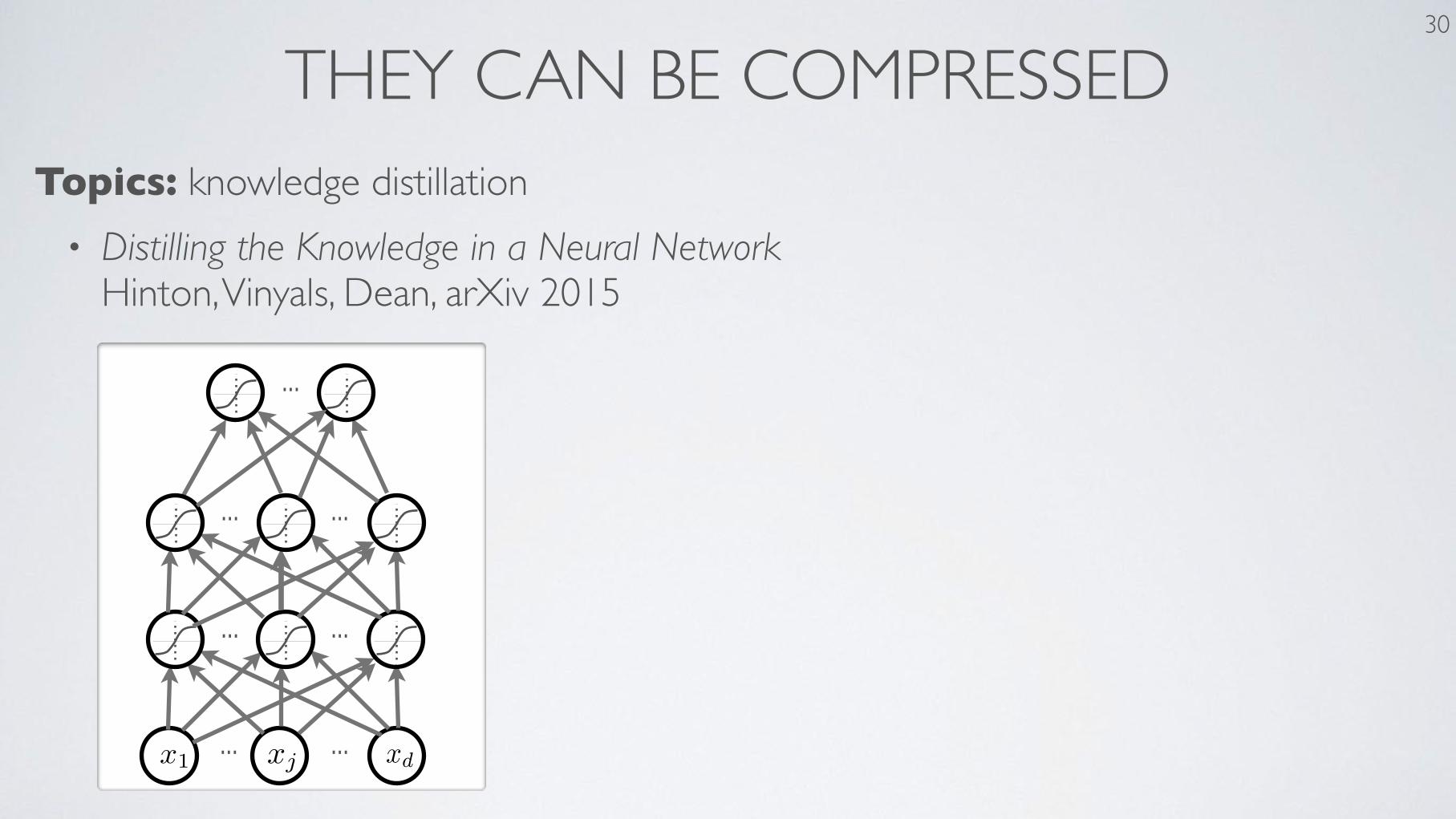
THEY CAN BE COMPRESSED 30
Topics: knowledge distillation• Distilling the Knowledge in a Neural Network
Hinton, Vinyals, Dean, arXiv 2015
...
Feedforward neural network
Hugo Larochelle
Departement d’informatiqueUniversite de Sherbrooke
September 6, 2012
Abstract
Math for my slides “Feedforward neural network”.
• a(x) = b+P
i wixi = b+w>x
• h(x) = g(a(x)) = g(b+P
i wixi)
• x1 xd
• w
• {
• g(·) b
• h(x) = g(a(x))
• a(x) = b(1) +W(1)x⇣a(x)i = b(1)i
Pj W
(1)i,j xj
⌘
• o(x) = g(out)(b(2) +w(2)>x)
1
...
Feedforward neural network
Hugo Larochelle
Departement d’informatiqueUniversite de Sherbrooke
September 6, 2012
Abstract
Math for my slides “Feedforward neural network”.
• a(x) = b+P
i wixi = b+w>x
• h(x) = g(a(x)) = g(b+P
i wixi)
• x1 xd b w1 wd
• w
• {
• g(a) = a
• g(a) = sigm(a) = 11+exp(�a)
• g(a) = tanh(a) = exp(a)�exp(�a)exp(a)+exp(�a) = exp(2a)�1
exp(2a)+1
• g(a) = max(0, a)
• g(a) = reclin(a) = max(0, a)
• g(·) b
• W (1)i,j b(1)i xj h(x)i
• h(x) = g(a(x))
• a(x) = b(1) +W(1)x⇣a(x)i = b(1)i
Pj W
(1)i,j xj
⌘
• o(x) = g(out)(b(2) +w(2)>x)
1
......
......
...

THEY CAN BE COMPRESSED 31
Topics: knowledge distillation• Distilling the Knowledge in a Neural Network
Hinton, Vinyals, Dean, arXiv 2015
...
Feedforward neural network
Hugo Larochelle
Departement d’informatiqueUniversite de Sherbrooke
September 6, 2012
Abstract
Math for my slides “Feedforward neural network”.
• a(x) = b+P
i wixi = b+w>x
• h(x) = g(a(x)) = g(b+P
i wixi)
• x1 xd
• w
• {
• g(·) b
• h(x) = g(a(x))
• a(x) = b(1) +W(1)x⇣a(x)i = b(1)i
Pj W
(1)i,j xj
⌘
• o(x) = g(out)(b(2) +w(2)>x)
1
Feedforward neural network
Hugo Larochelle
Departement d’informatiqueUniversite de Sherbrooke
September 6, 2012
Abstract
Math for my slides “Feedforward neural network”.
• a(x) = b+P
i wixi = b+w>x
• h(x) = g(a(x)) = g(b+P
i wixi)
• x1 xd
• w
• {
• g(·) b
• h(x) = g(a(x))
• a(x) = b(1) +W(1)x⇣a(x)i = b(1)i
Pj W
(1)i,j xj
⌘
• o(x) = g(out)(b(2) +w(2)>x)
1
...
Feedforward neural network
Hugo Larochelle
Departement d’informatiqueUniversite de Sherbrooke
September 6, 2012
Abstract
Math for my slides “Feedforward neural network”.
• a(x) = b+P
i wixi = b+w>x
• h(x) = g(a(x)) = g(b+P
i wixi)
• x1 xd b w1 wd
• w
• {
• g(a) = a
• g(a) = sigm(a) = 11+exp(�a)
• g(a) = tanh(a) = exp(a)�exp(�a)exp(a)+exp(�a) = exp(2a)�1
exp(2a)+1
• g(a) = max(0, a)
• g(a) = reclin(a) = max(0, a)
• g(·) b
• W (1)i,j b(1)i xj h(x)i
• h(x) = g(a(x))
• a(x) = b(1) +W(1)x⇣a(x)i = b(1)i
Pj W
(1)i,j xj
⌘
• o(x) = g(out)(b(2) +w(2)>x)
1
......
......
...
...
Feedforward neural network
Hugo Larochelle
Departement d’informatiqueUniversite de Sherbrooke
September 6, 2012
Abstract
Math for my slides “Feedforward neural network”.
• a(x) = b+P
i wixi = b+w>x
• h(x) = g(a(x)) = g(b+P
i wixi)
• x1 xd
• w
• {
• g(·) b
• h(x) = g(a(x))
• a(x) = b(1) +W(1)x⇣a(x)i = b(1)i
Pj W
(1)i,j xj
⌘
• o(x) = g(out)(b(2) +w(2)>x)
1
...
Feedforward neural network
Hugo Larochelle
Departement d’informatiqueUniversite de Sherbrooke
September 6, 2012
Abstract
Math for my slides “Feedforward neural network”.
• a(x) = b+P
i wixi = b+w>x
• h(x) = g(a(x)) = g(b+P
i wixi)
• x1 xd b w1 wd
• w
• {
• g(a) = a
• g(a) = sigm(a) = 11+exp(�a)
• g(a) = tanh(a) = exp(a)�exp(�a)exp(a)+exp(�a) = exp(2a)�1
exp(2a)+1
• g(a) = max(0, a)
• g(a) = reclin(a) = max(0, a)
• g(·) b
• W (1)i,j b(1)i xj h(x)i
• h(x) = g(a(x))
• a(x) = b(1) +W(1)x⇣a(x)i = b(1)i
Pj W
(1)i,j xj
⌘
• o(x) = g(out)(b(2) +w(2)>x)
1
...
...
...

THEY CAN BE COMPRESSED 32
Topics: knowledge distillation• Distilling the Knowledge in a Neural Network
Hinton, Vinyals, Dean, arXiv 2015
...
Feedforward neural network
Hugo Larochelle
Departement d’informatiqueUniversite de Sherbrooke
September 6, 2012
Abstract
Math for my slides “Feedforward neural network”.
• a(x) = b+P
i wixi = b+w>x
• h(x) = g(a(x)) = g(b+P
i wixi)
• x1 xd
• w
• {
• g(·) b
• h(x) = g(a(x))
• a(x) = b(1) +W(1)x⇣a(x)i = b(1)i
Pj W
(1)i,j xj
⌘
• o(x) = g(out)(b(2) +w(2)>x)
1
Feedforward neural network
Hugo Larochelle
Departement d’informatiqueUniversite de Sherbrooke
September 6, 2012
Abstract
Math for my slides “Feedforward neural network”.
• a(x) = b+P
i wixi = b+w>x
• h(x) = g(a(x)) = g(b+P
i wixi)
• x1 xd
• w
• {
• g(·) b
• h(x) = g(a(x))
• a(x) = b(1) +W(1)x⇣a(x)i = b(1)i
Pj W
(1)i,j xj
⌘
• o(x) = g(out)(b(2) +w(2)>x)
1
...
Feedforward neural network
Hugo Larochelle
Departement d’informatiqueUniversite de Sherbrooke
September 6, 2012
Abstract
Math for my slides “Feedforward neural network”.
• a(x) = b+P
i wixi = b+w>x
• h(x) = g(a(x)) = g(b+P
i wixi)
• x1 xd b w1 wd
• w
• {
• g(a) = a
• g(a) = sigm(a) = 11+exp(�a)
• g(a) = tanh(a) = exp(a)�exp(�a)exp(a)+exp(�a) = exp(2a)�1
exp(2a)+1
• g(a) = max(0, a)
• g(a) = reclin(a) = max(0, a)
• g(·) b
• W (1)i,j b(1)i xj h(x)i
• h(x) = g(a(x))
• a(x) = b(1) +W(1)x⇣a(x)i = b(1)i
Pj W
(1)i,j xj
⌘
• o(x) = g(out)(b(2) +w(2)>x)
1
......
......
...
...
Feedforward neural network
Hugo Larochelle
Departement d’informatiqueUniversite de Sherbrooke
September 6, 2012
Abstract
Math for my slides “Feedforward neural network”.
• a(x) = b+P
i wixi = b+w>x
• h(x) = g(a(x)) = g(b+P
i wixi)
• x1 xd
• w
• {
• g(·) b
• h(x) = g(a(x))
• a(x) = b(1) +W(1)x⇣a(x)i = b(1)i
Pj W
(1)i,j xj
⌘
• o(x) = g(out)(b(2) +w(2)>x)
1
Feedforward neural network
Hugo Larochelle
Departement d’informatiqueUniversite de Sherbrooke
September 6, 2012
Abstract
Math for my slides “Feedforward neural network”.
• a(x) = b+P
i wixi = b+w>x
• h(x) = g(a(x)) = g(b+P
i wixi)
• x1 xd
• w
• {
• g(·) b
• h(x) = g(a(x))
• a(x) = b(1) +W(1)x⇣a(x)i = b(1)i
Pj W
(1)i,j xj
⌘
• o(x) = g(out)(b(2) +w(2)>x)
1
...
Feedforward neural network
Hugo Larochelle
Departement d’informatiqueUniversite de Sherbrooke
September 6, 2012
Abstract
Math for my slides “Feedforward neural network”.
• a(x) = b+P
i wixi = b+w>x
• h(x) = g(a(x)) = g(b+P
i wixi)
• x1 xd b w1 wd
• w
• {
• g(a) = a
• g(a) = sigm(a) = 11+exp(�a)
• g(a) = tanh(a) = exp(a)�exp(�a)exp(a)+exp(�a) = exp(2a)�1
exp(2a)+1
• g(a) = max(0, a)
• g(a) = reclin(a) = max(0, a)
• g(·) b
• W (1)i,j b(1)i xj h(x)i
• h(x) = g(a(x))
• a(x) = b(1) +W(1)x⇣a(x)i = b(1)i
Pj W
(1)i,j xj
⌘
• o(x) = g(out)(b(2) +w(2)>x)
1
...
...
... y
THEY CAN BE COMPRESSED 33
Topics: knowledge distillation• Can successfully distill‣ a large neural network
‣ an ensemble of neural network
• Works better than training it from scratch!‣ Do Deep Nets Really Need to be Deep?
Jimmy Ba, Rich Caruana, NIPS 2014

THEY ARE INFLUENCED BY INITIALIZATION 34
Topics: impact of initialization• Why Does Unsupervised Pre-Training Help Deep Learning
Erhan, Bengio, Courville, Manzagol, Vincent, JMLR 2010
ERHAN, BENGIO, COURVILLE, MANZAGOL, VINCENT AND BENGIO
focus respectively on local9 and global structure.10 Each point is colored according to the trainingiteration, to help follow the trajectory movement.
−100 −80 −60 −40 −20 0 20 40 60 80 100−100
−80
−60
−40
−20
0
20
40
60
80
100
2 layers without pre−training
2 layers with pre−training
Figure 5: 2D visualizations with tSNE of the functions represented by 50 networks with and 50 net-works without pre-training, as supervised training proceeds over MNIST. See Section 6.3for an explanation. Color from dark blue to cyan and red indicates a progression in train-ing iterations (training is longer without pre-training). The plot shows models with 2hidden layers but results are similar with other depths.
What seems to come out of these visualizations is the following:
1. The pre-trained and not pre-trained models start and stay in different regions of functionspace.
2. From the visualization focusing on local structure (Figure 5) we see that all trajectories ofa given type (with pre-training or without) initially move together. However, at some point(after about 7 epochs) the different trajectories (corresponding to different random seeds)diverge (slowing down into elongated jets) and never get back close to each other (this ismore true for trajectories of networks without pre-training). This suggests that each trajectorymoves into a different apparent local minimum.11
9. t-Distributed Stochastic Neighbor Embedding, or tSNE, by van der Maaten and Hinton (2008), with the default pa-rameters available in the public implementation: http://ict.ewi.tudelft.nl/˜lvandermaaten/t-SNE.html.
10. Isomap by Tenenbaum et al. (2000), with one connected component.11. One may wonder if the divergence points correspond to a turning point in terms of overfitting. As shall be seen in
Figure 8, the test error does not improve much after the 7th epoch, which reinforces this hypothesis.
640

THEY ARE INFLUENCED BY FIRST EXAMPLES 35
Topics: impact of early examples• Why Does Unsupervised Pre-Training Help Deep Learning
Erhan, Bengio, Courville, Manzagol, Vincent, JMLR 2010
WHY DOES UNSUPERVISED PRE-TRAINING HELP DEEP LEARNING?
the first million examples (across 10 different random draws, sampling a different set of 1 millionexamples each time) and keep the other ones fixed. After training the (10) models, we measure thevariance (across the 10 draws) of the output of the networks on a fixed test set (i.e., we measure thevariance in function space). We then vary the next million examples in the same fashion, and so on,to see how much each of the ten parts of the training set influenced the final function.
Figure 13: Variance of the output of a trained network with 1 layer. The variance is computed asa function of the point at which we vary the training samples. Note that the 0.25 markcorresponds to the start of pre-training.
Figure 13 shows the outcome of such an analysis. The samples at the beginning15 do seem toinfluence the output of the networks more than the ones at the end. However, this variance is lowerfor the networks that have been pre-trained. In addition to that, one should note that the variance ofpre-trained network at 0.25 (i.e., the variance of the output as a function of the first samples used forsupervised training) is lower than the variance of the supervised network at 0.0. Such results implythat unsupervised pre-training can be seen as a sort of variance reduction technique, consistent witha regularization hypothesis. Finally, both networks are more influenced by the last examples usedfor optimization, which is simply due to the fact that we use stochastic gradient with a constantlearning rate, where the most recent examples’ gradient has a greater influence.
These results are consistent with what our hypothesis predicts: both the fact that early exampleshave greater influence (i.e., the variance is higher) and that pre-trained models seem to reduce thisvariance are in agreement with what we would have expected.
15. Which are unsupervised examples, for the red curve, until the 0.25 mark in Figure 13.
651

YET THEY FORGET WHAT THEY LEARNED 36
Topics: lifelong learning, continual learning• Overcoming Catastrophic Forgetting in Neural Networks
Kirkpatrick et al. PNAS 2017
Figure 2: Results on the permuted MNIST task. A: Training curves for three random permutations A, B and Cusing EWC(red), L2 regularization (green) and plain SGD(blue). Note that only EWC is capable of mantaininga high performance on old tasks, while retaining the ability to learn new tasks. B: Average performance acrossall tasks using EWC (red) or SGD with dropout regularization (blue). The dashed line shows the performanceon a single task only. C: Similarity between the Fisher information matrices as a function of network depth fortwo different amounts of permutation. Either a small square of 8x8 pixels in the middle of the image is permuted(grey) or a large square of 26x26 pixels is permuted (black). Note how the more different the tasks are, thesmaller the overlap in Fisher information matrices in early layers.
of subsequent tasks. This problem cannot be countered by regularizing the network with a fixedquadratic constraint for each weight (green curves, L2 regularization): here, the performance in taskA degrades much less severely, but task B cannot be learned properly as the constraint protects allweights equally, leaving little spare capacity for learning on B. However, when we use EWC, and thustake into account how important each weight is to task A, the network can learn task B well withoutforgetting task A (red curves). This is exactly the expected behaviour described diagrammatically inFigure 1.
Previous attempts to solve the continual learning problem for deep neural networks have relied uponcareful choice of network hyperparameters, together with other standard regularization methods, inorder to mitigate catastrophic forgetting. However, on this task, they have only achieved reasonableresults on up to two random permutations [Srivastava et al., 2013, Goodfellow et al., 2014]. Using asimilar cross-validated hyperparameter search as [Goodfellow et al., 2014], we compared traditionaldropout regularization to EWC. We find that stochastic gradient descent with dropout regularizationalone is limited, and that it does not scale to more tasks (Figure 2B). In contrast, EWC allows a largenumber of tasks to be learned in sequence, with only modest growth in the error rates.
Given that EWC allows the network to effectively squeeze in more functionality into a network withfixed capacity, we might ask whether it allocates completely separate parts of the network for eachtask, or whether capacity is used in a more efficient fashion by sharing representation. To assess this,we determined whether each task depends on the same sets of weights, by measuring the overlapbetween pairs of tasks’ respective Fisher information matrices (see Appendix 4.3). A small overlapmeans that the two tasks depend on different sets of weights (i.e. EWC subdivides the network’sweights for different tasks); a large overlap indicates that weights are being used for both the two tasks(i.e. EWC enables sharing of representations). Figure 2C shows the overlap as a function of depth.As a simple control, when a network is trained on two tasks which are very similar to each other(two versions of MNIST where only a few pixels are permutated), the tasks depend on similar sets ofweights throughout the whole network (grey curve). When then the two tasks are more dissimilarfrom each other, the network begins to allocate separate capacity (i.e. weights) for the two tasks(black line). Nevertheless, even for the large permutations, the layers of the network closer to theoutput are indeed being reused for both tasks. This reflects the fact that the permutations make theinput domain very different, but the output domain (i.e. the class labels) is shared.
2.2 EWC allows continual learning in a reinforcement learning context
We next tested whether elastic weight consolidation could support continual learning in the farmore demanding reinforcement learning (RL) domain. In RL, agents dynamically interact withthe environment in order to develop a policy that maximizes cumulative future reward. We askedwhether Deep Q Networks (DQNs)—an architecture that has achieved impressive successes in suchchallenging RL settings [Mnih et al., 2015]—could be harnessed with EWC to successfully supportcontinual learning in the classic Atari 2600 task set [Bellemare et al., 2013]. Specifically, each
4

SO THERE IS A LOT MORE TO UNDERSTAND!!
37

MERCI!
38