Geoffrey Hinton Nitish Srivastava, Kevin Swersky Tijmen Tieleman Abdel-rahman Mohamed

Neural Networks for Machine Learning

Lecture 9a Overview of ways to improve generalization

Reminder: Overfitting

•  The training data contains information about the regularities in the mapping from input to output. But it also contains sampling error. –  There will be accidental regularities just because of

the particular training cases that were chosen. •  When we fit the model, it cannot tell which regularities

are real and which are caused by sampling error. –  So it fits both kinds of regularity. If the model is very

flexible it can model the sampling error really well.

Preventing overfitting

•  Approach 1: Get more data! –  Almost always the best bet if you

have enough compute power to train on more data.

•  Approach 2: Use a model that has the right capacity: –  enough to fit the true regularities. –  not enough to also fit spurious

regularities (if they are weaker).

•  Approach 3: Average many different models. –  Use models with different forms. –  Or train the model on different

subsets of the training data (this is called “bagging”).

•  Approach 4: (Bayesian) Use a single neural network architecture, but average the predictions made by many different weight vectors.

Some ways to limit the capacity of a neural net

•  The capacity can be controlled in many ways: –  Architecture: Limit the number of hidden layers and the number

of units per layer. –  Early stopping: Start with small weights and stop the learning

before it overfits. –  Weight-decay: Penalize large weights using penalties or

constraints on their squared values (L2 penalty) or absolute values (L1 penalty).

–  Noise: Add noise to the weights or the activities. •  Typically, a combination of several of these methods is used.

How to choose meta parameters that control capacity (like the number of hidden units or the size of the weight penalty)

•  The wrong method is to try lots of alternatives and see which gives the best performance on the test set. –  This is easy to do, but it gives a

false impression of how well the method works.

–  The settings that work best on the test set are unlikely to work as well on a new test set drawn from the same distribution.

•  An extreme example: Suppose the test set has random answers that do not depend on the input. –  The best architecture will

do better than chance on the test set.

–  But it cannot be expected to do better than chance on a new test set.

Cross-validation: A better way to choose meta parameters

•  Divide the total dataset into three subsets: –  Training data is used for learning the parameters of the model. –  Validation data is not used for learning but is used for deciding

what settings of the meta parameters work best. –  Test data is used to get a final, unbiased estimate of how well the

network works. We expect this estimate to be worse than on the validation data.

•  We could divide the total dataset into one final test set and N other subsets and train on all but one of those subsets to get N different estimates of the validation error rate. –  This is called N-fold cross-validation. –  The N estimates are not independent.

Preventing overfitting by early stopping

•  If we have lots of data and a big model, its very expensive to keep re-training it with different sized penalties on the weights.

•  It is much cheaper to start with very small weights and let them grow until the performance on the validation set starts getting worse. –  But it can be hard to decide when performance is getting worse.

•  The capacity of the model is limited because the weights have not had time to grow big.

Why early stopping works

•  When the weights are very small, every hidden unit is in its linear range. –  So a net with a large layer of

hidden units is linear. –  It has no more capacity than

a linear net in which the inputs are directly connected to the outputs!

•  As the weights grow, the hidden units start using their non-linear ranges so the capacity grows.

outputs

inputs

W1

W2

Geoffrey Hinton Nitish Srivastava, Kevin Swersky Tijmen Tieleman Abdel-rahman Mohamed

Neural Networks for Machine Learning

Lecture 9b Limiting the size of the weights

Limiting the size of the weights

•  The standard L2 weight penalty involves adding an extra term to the cost function that penalizes the squared weights. –  This keeps the weights small

unless they have big error derivatives.

w

C when ∂C∂wi

= 0, wi = −1

λ∂E∂wi

C = E + λ2

wi2

i∑

∂C∂wi

=∂E∂wi

+λwi

The effect of L2 weight cost

•  It prevents the network from using weights that it does not need. –  This can often improve generalization a lot

because it helps to stop the network from fitting the sampling error.

–  It makes a smoother model in which the output changes more slowly as the input changes.

•  If the network has two very similar inputs it prefers to put half the weight on each rather than all the weight on one.

w/2 w/2

w 0

Other kinds of weight penalty

•  Sometimes it works better to penalize the absolute values of the weights. –  This can make many weights

exactly equal to zero which helps interpretation a lot.

•  Sometimes it works better to use a weight penalty that has negligible effect on large weights. –  This allows a few large weights.

0

0

Weight penalties vs weight constraints •  We usually penalize the

squared value of each weight separately.

•  Instead, we can put a constraint on the maximum squared length of the incoming weight vector of each unit. –  If an update violates this

constraint, we scale down the vector of incoming weights to the allowed length.

•  Weight constraints have several advantages over weight penalties. –  Its easier to set a sensible value. –  They prevent hidden units getting

stuck near zero. –  They prevent weights exploding.

•  When a unit hits it’s limit, the effective weight penalty on all of it’s weights is determined by the big gradients. –  This is more effective than a fixed

penalty at pushing irrelevant weights towards zero.

Geoffrey Hinton Nitish Srivastava, Kevin Swersky Tijmen Tieleman Abdel-rahman Mohamed

Neural Networks for Machine Learning

Lecture 9c Using noise as a regularizer

L2 weight-decay via noisy inputs •  Suppose we add Gaussian noise to the inputs.

–  The variance of the noise is amplified by the squared weight before going into the next layer.

•  In a simple net with a linear output unit directly connected to the inputs, the amplified noise gets added to the output.

•  This makes an additive contribution to the squared error. –  So minimizing the squared error tends to

minimize the squared weights when the inputs are noisy.

i

j

xi + N(0,σ i2 )

wi

yj + N(0,wi2σ i

2 )

Gaussian noise

ynoisy = wii∑ xi + wiεi

i∑ where εi is sampled from N(0,σ i

2 )

So is equivalent to an L2 penalty σ i2

because εi is independent of ε jand εi is independent of (y− t)

E (ynoisy − t)2"#

$%= E y+ wiεi

i∑ − t

'

())

*

+,,

2"

#

--

$

%

.

.= E (y− t)+ wiεi

i∑

'

())

*

+,,

2"

#

--

$

%

.

.

= (y− t)2 +E 2(y− t) wiεii∑

#

$%%

&

'((+E wiεi

i∑)

*++

,

-..

2#

$

%%

&

'

((

= (y− t)2 +E wi2εi2

i∑#

$%%

&

'((

= (y− t)2 + wi2σ i

2

i∑

output on one case

Noisy weights in more complex nets

•  Adding Gaussian noise to the weights of a multilayer non-linear neural net is not exactly equivalent to using an L2 weight penalty. –  It may work better, especially in recurrent

networks. –  Alex Graves’ recurrent net that recognizes

handwriting, works significantly better if noise is added to the weights.

Using noise in the activities as a regularizer •  Suppose we use backpropagation to

train a multilayer neural net composed of logistic units. –  What happens if we make the units

binary and stochastic on the forward pass, but do the backward pass as if we had done the forward pass “properly”?

•  It does worse on the training set and trains considerably slower. –  But it does significantly better on

the test set! (unpublished result).

p(s =1) = 1

1+ e−z

0.5

0 0

1

z

p

Geoffrey Hinton Nitish Srivastava, Kevin Swersky Tijmen Tieleman Abdel-rahman Mohamed

Neural Networks for Machine Learning

Lecture 9d Introduction to the Bayesian Approach

The Bayesian framework •  The Bayesian framework assumes that we always have a prior

distribution for everything. –  The prior may be very vague. –  When we see some data, we combine our prior distribution

with a likelihood term to get a posterior distribution. –  The likelihood term takes into account how probable the

observed data is given the parameters of the model. •  It favors parameter settings that make the data likely. •  It fights the prior •  With enough data the likelihood terms always wins.

A coin tossing example •  Suppose we know nothing about coins except that each

tossing event produces a head with some unknown probability p and a tail with probability 1-p. –  Our model of a coin has one parameter, p.

•  Suppose we observe 100 tosses and there are 53 heads. What is p?

•  The frequentist answer (also called maximum likelihood): Pick the value of p that makes the observation of 53 heads and 47 tails most probable. –  This value is p=0.53

A coin tossing example: the math

P(D) = p53(1− p)47probability of a particular sequence containing 53 heads and 47 tails.

dP(D)dp

= 53p52(1− p)47 − 47p53(1− p)46

=53p−471− p

"

#$

%

&' p53(1− p)47()

*+

= 0 if p = .53

Some problems with picking the parameters that are most likely to generate the data

•  What if we only tossed the coin once and we got 1 head? –  Is p=1 a sensible

answer? –  Surely p=0.5 is a

much better answer.

•  Is it reasonable to give a single answer? –  If we don’t have much data,

we are unsure about p. –  Our computations of

probabilities will work much better if we take this uncertainty into account.

Using a distribution over parameter values

•  Start with a prior distribution over p. In this case we used a uniform distribution.

•  Multiply the prior probability of each parameter value by the probability of observing a head given that value.

•  Then scale up all of the probability densities so that their integral comes to 1. This gives the posterior distribution.

probability density

p area=1

area=1

0 1

1

1

2

probability density

probability density

Lets do it again: Suppose we get a tail

•  Start with a prior distribution over p.

•  Multiply the prior probability of each parameter value by the probability of observing a tail given that value.

•  Then renormalize to get the posterior distribution. Look how sensible it is!

probability density

p area=1

area=1

0 1

1

2

Lets do it another 98 times

•  After 53 heads and 47 tails we get a very sensible posterior distribution that has its peak at 0.53 (assuming a uniform prior).

probability density

p

area=1

0 1

1

2

Bayes Theorem

p(D)p(W |D) = p(D,W ) = p(W )p(D |W )

prior probability of weight vector W

posterior probability of weight vector W given training data D

probability of observed data given W

joint probability conditional probability

p(W |D) =p(W ) p(D |W )

p(D)

p(W )p(D |W )W∫

Geoffrey Hinton Nitish Srivastava, Kevin Swersky Tijmen Tieleman Abdel-rahman Mohamed

Neural Networks for Machine Learning

Lecture 9e The Bayesian interpretation of weight decay

Supervised Maximum Likelihood Learning •  Finding a weight vector that

minimizes the squared residuals is equivalent to finding a weight vector that maximizes the log probability density of the correct answer.

•  We assume the answer is generated by adding Gaussian noise to the output of the neural network.

t correct answer

y model’s estimate of most probable value

Supervised Maximum Likelihood Learning

p(tc | yc ) =12πσ

e−(tc−yc )

2

2σ 2

yc = f (inputc , W )output of the net Gaussian distribution centered at the net’s output

probability density of the target value given the net’s output plus Gaussian noise

Cost

Minimizing squared error is the same as maximizing log prob under a Gaussian.

− log p(tc | yc ) = k +(tc − yc )

2

2σ 2

MAP: Maximum a Posteriori •  The proper Bayesian approach

is to find the full posterior distribution over all possible weight vectors. –  If we have more than a

handful of weights this is hopelessly difficult for a non-linear net.

–  Bayesians have all sort of clever tricks for approximating this horrendous distribution.

•  Suppose we just try to find the most probable weight vector. –  We can find an optimum by

starting with a random weight vector and then adjusting it in the direction that improves p( W | D ).

–  But it’s only a local optimum. •  It is easier to work in the log

domain. If we want to minimize a cost we use negative log probs

Why we maximize sums of log probabilities

•  We want to maximize the product of the probabilities of the producing the target values on all the different training cases. –  Assume the output errors on different cases, c, are independent.

•  Because the log function is monotonic, it does not change where the maxima are. So we can maximize sums of log probabilities

p(D |W ) = p(tcc∏ |W ) = p tc | f (inputc,W )( )

c∏

log p(D |W ) = log p(tcc∑ |W )

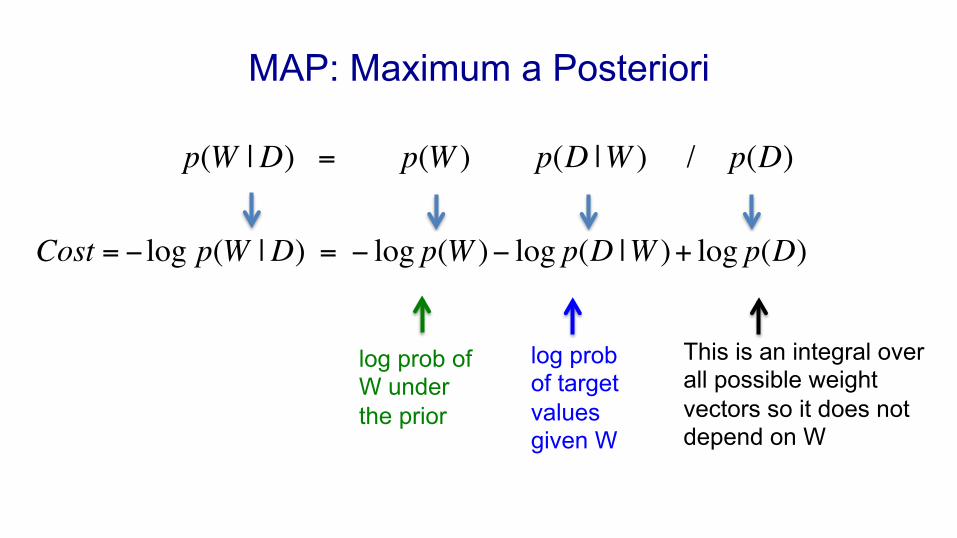
MAP: Maximum a Posteriori

p(W |D) = p(W ) p(D |W ) / p(D)

This is an integral over all possible weight vectors so it does not depend on W

log prob of W under the prior

log prob of target values given W

Cost = − log p(W |D) = − log p(W )− log p(D |W )+ log p(D)

The log probability of a weight under its prior

•  Minimizing the squared weights is equivalent to maximizing the log probability of the weights under a zero-mean Gaussian prior.

w 0

p(w) p(w) = 1

2πσe−w2

2σW2

− log p(w) = w2

2σW2 + k

The Bayesian interpretation of weight decay

− log p(W |D) = − log p(D |W ) − log p(W ) + log p(D)

assuming a Gaussian prior for the weights

assuming that the model makes a Gaussian prediction

constant

So the correct value of the weight decay parameter is the ratio of two variances. It’s not just an arbitrary hack.

C = E +σD2

σW2 wi

2

i∑

C* = 1

2σD2 (yc

c∑ − tc )

2 + 1

2σW2 wi

2

i∑

Geoffrey Hinton Nitish Srivastava, Kevin Swersky Tijmen Tieleman Abdel-rahman Mohamed

Neural Networks for Machine Learning

Lecture 9f MacKay’s quick and dirty method of fixing

weight costs

Estimating the variance of the output noise

•  After we have learned a model that minimizes the squared error, we can find the best value for the output noise. –  The best value is the one that maximizes the probability of

producing exactly the correct answers after adding Gaussian noise to the output produced by the neural net.

–  The best value is found by simply using the variance of the residual errors.

Estimating the variance of the Gaussian prior on the weights

•  After learning a model with some initial choice of variance for the weight prior, we could do a dirty trick called “empirical Bayes”. –  Set the variance of the Gaussian prior to be whatever makes the

weights that the model learned most likely. •  i.e. use the data itself to decide what your prior is!

–  This is done by simply fitting a zero-mean Gaussian to the one-dimensional distribution of the learned weight values.

•  We could easily learn different variances for different sets of weights.

•  We don’t need a validation set!

MacKay’s quick and dirty method of choosing the ratio of the noise variance to the weight prior variance.

•  Start with guesses for both the noise variance and the weight prior variance.

•  While not yet bored –  Do some learning using the ratio of the variances as the weight

penalty coefficient. –  Reset the noise variance to be the variance of the residual errors. –  Reset the weight prior variance to be the variance of the

distribution of the actual learned weights. •  Go back to the start of this loop.