Neural networks (not in book)

Another approach to classification is neural networks. Neural networkswere developed in the 1980s as a way to model how learning occurs in thebrain. There was therefore wide interest in neural networks amongresearchers in cognitive science and artificial intelligence. It is also ofinterest just as a classification technqiue, without necessarily havingconnections to understanding the brain or artificial intelligence.

April 8, 2015 1 / 40

Neural networks

April 8, 2015 2 / 40

Neural networks

The motivation for neural networks comes from thinking about the brain.The brain has cells called neurons which have multiple inputs (dendrites),and a single output (axon). Brain cells are connected to each other so thatthe output from one cell can part of the input in another neuron. Theconnections between axons and dendrites and called synapses. A crudemodel for this system is that there are multiple continuous or discreteinputs and single binary output. The output is that either the axon fires ordoesn’t fire. Whether or not the axon fires depends upon the strength ofthe inputs, which crudely could be determined by whether the sum of theinputs in the dendrites reaches some threshold.

April 8, 2015 3 / 40

Neural networks

When the axon fires, it discharges an electrical pulse. This gets distributedto other dendrites that are connected via synapses to the axon, which inturn can cause other neurons to fire or not fire. Eventually, this processingcan result in, for example, perceptual inputs (e.g., visual images, sounds,etc.) to be classified and possibly lead to actions (motor activity).

How much a neuron firing affects neurons downstream is weighted bybiological factors such as neurotransmitters in the synapses, and can bemodified by experience (i.e., learning).

April 8, 2015 4 / 40

Neural network

In an artificial neural network model, an array of neurons receives inputfrom multiple variables. The variables are weighted, so that each neurongets some linear combination of the input signals, and either fires ordoesn’t fire depending on the weighted sum of the inputs.

April 8, 2015 5 / 40

Neural networks

April 8, 2015 6 / 40

Neural networks

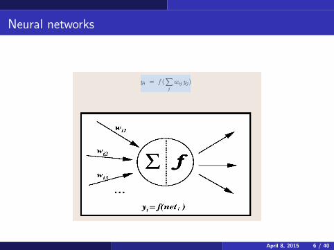
Generally, neuron i fires if the total input∑

j wijxj is greater than somethreshold. Several neurons are together in the same network. If the data islinearly separable, then you can have just a single layer of neuronsconnected to an output.

Two sets of vectors y1, . . . , yn and x1, . . . , xm are called linearlysepararable if weights exist such that∑

j

wijyj ≥ θ for all i ∈ {1, . . . , n}

∑j

wijxj < θ for alli ∈ {1, . . . ,m}

April 8, 2015 7 / 40

Neural networks

April 8, 2015 8 / 40

Neural networks

Neural networks can also be used for more complicated classifications,including nonlinear functions, and what are called XOR functions. Forexample, rather than classifying an observation as 1 versus 0 based onwhether a linear combination is high or low, it could could classified as 1 ifone variable is high or the other variable is high, but not both of them arehigh.

April 8, 2015 9 / 40

Neural networks

April 8, 2015 10 / 40

Neural networks

Critical to how neural networks function is how to get the weights. Oftenthe weights are initially randomized (for example, numbers between 0 and1), and then they are gradually improved through training or learning.There are different types of learning, called supervised, unsupervised, andreinforcement.

In supervised learning, a correct classification is known on some trainingdata. The system’s weights are updated when the networks classification iscompared to the training set so as to improve future performance.

In unsupervised learning, the correct classification is unknown. This ismore like the situtaiton in clustering.

In reinforcement, the correct classification isn’t given, but the system isrewarded depending on how well it performed.

April 8, 2015 11 / 40

Neural networks

To illustrate supervised learning in a single-layer network, we have a targetoutput t, and the actually output

o = f

n∑j=1

w1jxj , . . . ,

p∑j=1

wpjxj

The error is then

E = t − o

We have some learning rate parameter r , and the weights are adjusted by

∆wi = r(t − o)xi

April 8, 2015 12 / 40

Neural networks

April 8, 2015 13 / 40

Neural networks

To take an example, suppose a single layer network has two input nodes.The two input nodes have weights w1 = .2 and w2 = .3, and we user = 0.2. Suppose we train on one observation which should be classified asa 1 (i.e., the output neuron should fire). If the input is (x1, x2) = (1, 1),then the combined weight is

w1x1 + w2x2 = 0.2 + 0.3 = 0.5

so the neuron doesn’t fire. The change in weights is

∆w1 = (0.2)(1− 0)(1)− 0.2, ∆w2 = (0.2)(1− 0)(1) = 0.1

so each weight increases by 0.2. The new weights are w1 = 0.4 andw2 = 0.5.

April 8, 2015 14 / 40

Neural networks

To continue the example, suppose another training observation occurs,and the target is again 1, but the observation is

(x1, x2) = (0, 1)

In this case, the output using the new weights is

w1x1 + w2x2 = 0 + 0.5 < 1.0

so again the output is 0. In this case

∆w1 = (0.2)(1− 0)(0) = 0, ∆w2 = (0.2)(1− 0)(1) = 0.2

Now we increase the weight for w2 but not for w1, so the new weights arew1 = 0.4 and w2 = 0.7. For new input, the neural network will classify theobservation as 1 if the input is (1, 1) but will otherwise classify it as 0.

April 8, 2015 15 / 40

Neural networks

Assuming that you have a neural network sufficiently complex to correctlyclassify all training data, you can go through the data again, re-updatingweights until all observations are correctly classified. If the data is toocomplex (e.g., not linearly separable for a single-layer network), then youneed a stopping rule such as a maximum number of iterations beforefinishing the training.

A common modification to this type of network is to have a bias inputunit, x0 that always fires regardless of the input unit. Its weight can still bemodified, so that if the weight is 0, you have an unbiased system; howeverhaving the bias unit can be helpful in make the classifications more flexible.

April 8, 2015 16 / 40

Neural networks

April 8, 2015 17 / 40

Neural networks

It is possible to overtrain a network, in which case it’s rules becomeoptimized to the training data but might not perform well on new data. Itis therefore useful to have training data and validation data to be sure thenetwork will perform well on new data.

April 8, 2015 18 / 40

Neural networks

April 8, 2015 19 / 40

Neural networks

For multi-layer networks, the methods for updated the weights is morecomplicated. The most common approach is called backpropogation.

April 8, 2015 20 / 40

Neural networks

April 8, 2015 21 / 40

Neural networks

April 8, 2015 22 / 40

Neural networks

April 8, 2015 23 / 40

Neural networks

April 8, 2015 24 / 40

Neural networks

The backpropogration rule requires derivatives of the f functions.Previously, we considered this function to be an indicator equal to 1 if theweighted sum of the inputs was greater than some threshold. To have afunction with a derivative, you can instead have a sigmoid function (forexample).

In the diagrams, η is used as the learning rate parameter. This can be afunction of time (or iteration) in the network, so that at first it updatesweights with bigger increments, then settles down over time.

April 8, 2015 25 / 40

Neural networks

An example with the chile data is

> library(nnet)

> target <- c(rep(0,11),rep(1,11))

> a <- nnet(target ~ y[,1] + y[,2],size=3)

> summary(a)

a 2-3-1 network with 13 weights

options were -

b->h1 i1->h1 i2->h1

32.94 7.00 -51.06

b->h2 i1->h2 i2->h2

-99.17 -12.47 77.75

b->h3 i1->h3 i2->h3

-1.92 -8.67 -6.18

b->o h1->o h2->o h3->o

38.95 -3.11 -40.56 -2.85

April 8, 2015 26 / 40

This created a network with two inputs plus a bias node, a 3-node hiddenlayer, and 1 output. The summary gives the weights, for example theweight from the bias node to hidden node 1 is 32.94. To get an idea ofthe performance, type

> summary(a)

> a$fitted.values

[,1]

1 0.5000790274

2 0.1663292192

3 0.1663292192

4 0.1663292192

5 0.1663292192

6 0.1663292192

7 0.1663292192

8 0.1663292192

9 0.1667868688

10 0.1683388180

11 0.1663292192

12 0.9901308104

13 0.1663292192

There are two chiles misclassified from Cochiti (only one is shown here,observation 13) and two that have essentially 50% weight (e.g.,observation 1)– so the network couldn’t classify them.

April 8, 2015 27 / 40

Logistic regression as a classifier

Logistic regression might not appear to be a multivariate technique sincewe have a single response (category as 1 or 2) and several explanatoryvariables. However, the way data is often collected, we have two groups,the response, which are known (e.g., cases and controls), and we collectdata on the explanatory variables.

It also makes sense to compare logistic regression to other classificationmethods since it is often applied to the same types of data.

April 8, 2015 28 / 40

Logistic regression

The goal in logistic regression as a classifier is to give a probability that anew observation belongs to a given class given the covariates. Again wecan use techniques such as training and validation sets or resubstitutionrates to estimate the error rate for a logistic regression classifier.

April 8, 2015 29 / 40

Logistic regression

Logistic regression, similar to regression, has a vector of coefficientsβ = (β0, β1, . . . , βp) for the covariates (1, x1, x2, . . . , xp), where β0 is thecoefficient for an intercept term.

The probabilities are modeled as

P(yi = 0|xi ) =1

1 + exp(β0 +∑p

j=1 βjxij)

P(yi = 1|xi ) =exp(β0 +

∑pj=1 βjxj)

1 + exp(β0 +∑p

j=1 βjxij)

April 8, 2015 30 / 40

Logistic regression

We can think of β0 as being similar to a bias term in neural networks. Ifxi = 0, then the probability that yi = 0 is

1

1 + exp(β0 + 0)=

1

1 + exp(β0)

For example, if β0 = .1, then P(yi = 0) = .475. When β0 = .2, thisprobability is 0.45. The larger the value of β0, the more predisposed theclassifier is to category 1 instead of category 0.

April 8, 2015 31 / 40

Logistic regression

Using the logistic function,

σ(z) =1

1 + exp(−z)

we can write the probabilities as

P(yi = 0|xi ) = σ

−β0 +

p∑j=1

βixij

P(yi = 1|xi ) = 1− P(yi = 0|xi )

The logistic function σ(z) is S-shaped and is positive between 0 and 1.

April 8, 2015 32 / 40

Logistic regression

Another interpretation for the logistic regression model is that

P(yi = 1|xi )P(yi = 0|xi )

= exp

β0 +

p∑j=1

βjxij

and

logP(yi = 1|xi )P(yi = 0|xi )

= β0 +

p∑j=1

βjxij

This makes the right side look like an ordinary regression problem, whileon the left we have the log odds of being in class 1. We can think of oddsas transforming probabilities, which are between 0 and 1, to a numberbetween 0 and ∞, and the log-odds transforms probabilities to numbersbetween −∞ and ∞.

April 8, 2015 33 / 40

Logistic regression

The estimation of the weights β is a bit difficult and is done usingmaximum likelihood numerically. Logistic regression can be done in Rusing the function glm.

April 8, 2015 34 / 40

Logistic regression

> truth <- c(rep(0,11),rep(1,11))

> lr1 <- glm(truth ~ y[,1] + y[,2])

> summary(lr1)

Estimate Std. Error z value Pr(>|z|)

(Intercept) 14.3372 7.0332 2.038 0.0415 *

y[, 1] 0.5164 0.5766 0.896 0.3705

y[, 2] -6.6008 2.7367 -2.412 0.0159 *

---

Signif. codes: 0 *** 0.001 ** 0.01 * 0.05 . 0.1 1

(Dispersion parameter for binomial family taken to be 1)

Null deviance: 30.498 on 21 degrees of freedom

Residual deviance: 16.413 on 19 degrees of freedom

AIC: 22.413

Number of Fisher Scoring iterations: 6

April 8, 2015 35 / 40

Logistic regression in R

To interpret the output, note that the number of Fisher Scoring iterationsrefers to how difficult it was, in terms of the number of iterations, toestimate the covariates using an iterative numerical method.

The deviance normally refers to −2Λ. The residual deviance compares themodel with the predictors to the null hypothesis of β = 0, while the nulldeviance compares the likelihoods of the intercept only model (βj = 0 forj > 0) to the null model (βj = 0 for j ≥ 0).

April 8, 2015 36 / 40

Logistic regression in R

The results suggest that width but not legnth were signficant predictors ofclass membership. However, the main interest here is not in whichvariables are significant but rather what leads to the best prediction.However, including insignificant variables runs the risk of overfitting thedata, so one might prefer a model without length. However,cross-validation methods might be used to decide this rather than usualmodel selection methods based on p-values, AIC, etc.

To get a sense of how well the logistic regression classifies, we can look atthe fitted values first, which give the estimated probabilities of classmembership for group 1 (Cochiti).

April 8, 2015 37 / 40

Logistic regression in R

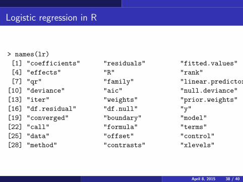
> names(lr)

[1] "coefficients" "residuals" "fitted.values"

[4] "effects" "R" "rank"

[7] "qr" "family" "linear.predictors"

[10] "deviance" "aic" "null.deviance"

[13] "iter" "weights" "prior.weights"

[16] "df.residual" "df.null" "y"

[19] "converged" "boundary" "model"

[22] "call" "formula" "terms"

[25] "data" "offset" "control"

[28] "method" "contrasts" "xlevels"

April 8, 2015 38 / 40

> t(t(lr1$fitted.values))

1 0.489107853

2 0.005758878

3 0.034092301

4 0.002176054

5 0.055848588

6 0.363563682

7 0.108225806

8 0.254209823

9 0.425129081

10 0.809937685

11 0.118241717

12 0.846548446

13 0.363563682

14 0.939374085

15 0.877176485

16 0.489107853

17 0.952513940

18 0.996929181

19 0.939374085

20 0.169012974

21 0.902396172

22 0.857711629

April 8, 2015 39 / 40

Logistic regression in R

In this case, observations 13, 16, and 20 were missclassified, withobservations 1 and 16 being close to 50%. The probability of being inclass 0 as a function of the covariates is

1

1 + exp(14.3372 + 0.5164Length − 6.6008Width

We could therefore make a plot showing whether an observation would beclassified as being Alcalde versus Cochiti as a function of Length andWidth for difference Length, Width combinations similar to the linear andquadratic classifiers done earlier. Another nice way to make the plot wouldbe to use shades of grey or a heat map (e.g., yellow to red) indicating theprobability of being classified into one of the two groups.

April 8, 2015 40 / 40

Logistic regression in R

To get a sense of what the black-and-white plot should look like, theboundary between the black and white regions is where the probabilities ofthe two groups are equal, so 0.5. This is where the odds is 1, andtherefore the log-odds is 0. Thus, on the boundary, we get

log

(p

1− p

)= 0 = 14.3372 + 0.5164Length − 6.6008Width

so we get a linear relationship between Length and Width. Thereforelogistic regression is really a linear classifier.

April 8, 2015 41 / 40

Logistic regression in R

To plot this, I used

> plot(c(6,12),c(1.5,4.5),type="n",xlab="Length",ylab="Width",cex.lab=1.3,cex.axis=1.3)

> prob <- function(x,y) {

return(1/(1+exp(14.3372 + 0.5164*x -6.6008*y)))

}

> length <- seq(6,12,.05)

> width <- (length - 6)/6 * 3 + 1.5

> for(i in 1:length(width)) {

> for(j in 1:length(width)) {

points(length[i],width[j],col=

paste("grey",round(100*(1-prob(length[i],width[j]))),sep="")

,cex=2,pch=15)

April 8, 2015 42 / 40

Logistic regression

April 8, 2015 43 / 40

Neural networks

April 8, 2015 44 / 40

Logistic regression in R

If we add Thickness as the third variable, the error rate actually getsworse, even using the substitution method. The method also has worseerror rates when Length is ignored. Using only width, the probabilities alsotend to be very moderate (close to .50).

April 8, 2015 45 / 40

> t(t(lr2$fitted.values))

[,1]

1 0.489964466

2 0.005259903

3 0.033651304

4 0.001951196

5 0.056337760

6 0.374129169

7 0.104482484

8 0.254654768

9 0.426804775

10 0.809361891

11 0.116277382

12 0.843432261

13 0.348551338

14 0.942023902

15 0.879010283

16 0.488579228

17 0.953083752

18 0.997011291

19 0.937312061

20 0.179098910

21 0.900990400

22 0.858031476

April 8, 2015 46 / 40

> t(t(lr3$fitted.values))

1 0.4452275

2 0.5818250

3 0.4452275

4 0.4068061

5 0.4068061

6 0.4843150

7 0.6008183

8 0.5235954

9 0.4647171

10 0.5818250

11 0.4941359

12 0.5625860

13 0.4843150

14 0.4843150

15 0.5431568

16 0.4452275

17 0.4647171

18 0.5039613

19 0.4843150

20 0.5625860

21 0.5235954

22 0.5059263

April 8, 2015 47 / 40