neural networks on the dynamic models - · pdf fileneural networks on the dynamic models...

Neural networks on the dynamic models

updating

Tiago Alberto Piedras Lopes, Omar Pereira de Andrade &

COPPE / Universidade Federal do Rio de Janeiro

Cou%z f a?W &9JO& CEP 27P4J-P70

Rio de Janeiro RJ Brasil

Email: [email protected] [email protected]

Affonso Lima Vianna Junior

M&D - Monitoragdo e Diagnose Ltda.

Incubadora de Empresas da COPPE/UFRJ

Cmxa f oaW 6&J63 CEf 2794J-970

Rio de Janeiro RJ Brasil

Email: m&d@incubadora. coppe. ufrj. br

Abstract

The correlation between theoretical and experimental models, which takes intoaccount the eigenfrequencies and eigenmodes obtaneid from an eigenvalueproblem and experimental modal analysis, permits to match the theorectical andexperimental results. Updating aims to modify the structural theoretical modelmatrices, such as mass and stiffness, to reproduce closely as possible themeasured response from the data. A new methodology for updating, based onneural networks, is proposed. The neural network will represent the inverse ofthe parameters sensitivity matrix. The input data for the neural network(changes on natural frequencies and modes) will correspond to thepertubation of measured parameters and the output neurons will representchanges on discrete masses or physical boundary conditions, associated to thepertubation paramenter. A spatial frame is used for evaluation of the neuralnetwork approach.

Transactions on Information and Communications Technologies vol 19 © 1998 WIT Press, www.witpress.com, ISSN 1743-3517

1 Introduction

The dynamic behavior modeling of structural systems involves,historically, two development fronts: the theoretical and theexperimental. The most usual theoretical models combine themechanical properties of the system (mass, stiffness and damping) in agroup of second order differential equations. Using computationalresources associated to well known numerical techniques, such as thefinite element method, the complex structural systems modeling becamefeasible. Nevertheless, these theoretical models present many limitationssuch as impracticability of high fine meshed discretizations, partialunknowledge of the system physical properties and others. Suchlimitations implicate in some model uncertainties which can make itinadequate for practical applications.

From the experimental viewpoint, the structural dynamic modelachievement is performed by parameters identification techniques.Generally, the experimental model consists, basically, in a group ofeigenvalues and eigenvectors, extracted from impulsive or generalresponse functions. The structure is represented by its natural modes andfrequencies and the modal damping coefficients. The recent solid stateeletronic and computation advances made easy the work of the expertsinvolved with experimental activities. The continuous development ofdata acquisition systems and digital signal processing permit to obtainmore accurate experimental dynamical models, faster and with lowercosts. By this way, once is ensured reliable test conditions, it is possibleto represent with sufficient confidence the strucutural dynamic behaviorover a limited frequency range. There is still many limitations associatedto a modal experimental test such as: numbers of sensors (practical andeconomical restrictions), actual influence of boundary conditions andmathematical inaccuracies derived from an incomplete structural modalbase.

The dynamic modeling techniques were extremely developed alongthe last two decades and are incorporated to the usual design proceduresof many industries and research centers around the world. The validationof theorectical models with aid of experimental results became more andmore common. However, the theorectical models complexity anddimension made practically impossible the theorectical and experimentalresults compatibility based only on engineering judgement (acumulatedexperience). The methodology which permits the correction andimprovement of theorectical models, based on experimental modalanalysis, is named dynamic models updating.

276


According to Mottershead[l], the inaccuracies in a theoretical modelcan be divided into three categories:1) errors by inaccuracies associated to the equations that govern the

system behavior;2) errors by deficient boundary conditions and not suitable assumptions;3) errors caused by inadequate mesh for the structure modeling.

The updating techniques will make possible the theorectical modelcorrection by adjusting the mass, stiffness and damping matrices,looking for an optimum correlation between measured and calculatedeigenvectors and eigenvalues. Such kind of procedure taking intoaccount errors due to second and third categories. A special attentionmust be paid to the fact that exist many possible solutions for this kind ofproblem, most of them without any physical meaning. Constraints mustbe applied to updating procedures for keeping the physicalcharacteristics of the structure Janter[2].

The dynamical model updating could depart from the hypothesis thatthe experimental data are perfect, without any kind of errors, but this factis not true. The experimental results also have uncertainties, causedmainly by noise, such as electromagnetic interference. Therefore, the

noise must be taking into account or filtered.

2 Dynamic Model Updating Techniques

From the correlation between the experimental and the theorectical data,

that consists in a qualitative and quantitative comparison between thetheorectical and the experimental models, the mass and stiffness matricescould be updated, assuming that the experimental results are reliable.The following methodologies are usually applied:• comparison of the natural frequencies: can be performed, for instance, bygraphical representation of the theorectical vs. experimental natural

frequencies. The ideal result is a 45° straight line starting at origin. If thepoints stay in a paralel line, it indicates a systematic error in thetheorectical model. If the points are sparsely distributed, there is a lowcorrelation between the experimental and the theorectical model.• comparison of the natural modes: the correlation between the theorecticaland experimental natural modes permits to obtain the best picture toevaluate the data. The nodal shape could be drawed side by side as a firstinformation about the natural modes. For detailed evaluation, isnecessary to quantify parameters which can produce relationshipsbetween the calculated and measured natural modes, such as MAC,COMAC and others.

277


The methods for updating dynamical models can be interpreted as anapplication of the parameters estimation theory in structures, where thestructural model numeric description is given by the finite elementsmethod matricial equations, as suggested by Natkes[3]. One direction forperforming the updating is based on a suitable penalty function: theobjective of maximize the correlation between the theorectical andexperimental model. This method permits a wide parameters selection tobe updated, but the optimization of non-linear functions require aiterative scheme with risk of non convergence and theorectical modelmust be reevaluated at each iteration. When the selected parametersvariations due to the iteration is small, a good estimative of thetheorectical model is accomplished. This method is usually based on aexpansion of eigenvalues and eigenvectors by means of truncated Taylorseries, to produce the following linear approximation:

8z=S,8p (l)

where 5p is the pertubation on selected parameters, 8z is the pertubation

on measured variable and S% is the parameters sensitivity matrix.The parameters sensitivity matrix contains the first derivative of the

eigenvectors and eigenvalues as function of the parameters that are beingconsidered. The calculation of this derivatives requires an efficientnumerical algorithm and high computational efforts. One formulation ofthe derivate of the eigenvalue A,j with respect to the parameter pj was

developed by Hemes* and the expression is the following:

Premultipling the expression (2) by <|>} and using the ortogonality

property related to the mass and the eigenvalue problem definition , thefollowing equation is obtained:

91, ,/9K . 9M^T— = 4>i %—-^i-Op . \UP j C

The expression (3) is easy to be calculated, because it requires onlyone eigenvalue and the respective eigenvector. The eigenvectorsderivative is harder to be calculated and several methods can be applied,

278


as listed in Hemes[4]. One of the methods involves the equation (2)together another one based on the orthogonality expression and generatesn+1 equations related to the nth eigenvector derivative to be determined.This group of equations is solved by pseudo-inverse technique, but thebandwidth caracteristcs are altered and hence the computational

efficiency is lost.Both natural frequencies and modes must be used on the updating

procedure in order to get better results. However, the natural modes mustbe handled carefully due to the experimental data inaccuracies. Afteracquiring the experimental data, is possible to guarantee an accuracybetter than 1% for the natural frequencies, but for the modes errors ofabout 20% are possible to occur in some components of the modalvector, as verified by Dascote[5]. Therefore, some appropriated criteriamust be applied to the natural modes evaluation in order to improve theaccuracy.

Normally, the number of parameters and measured variables in

equation (1) is not the same. Therefore, the sensivity matriz S* could bea not square matrix. If is considered the case when the number ofmeasured variables is larger than the number of selected parameters, thesolution is obtained by a quadratic error minimization and the updatedparameters with the minimum variance can be calculated by the

following equation:

& (4)

and the variance of the updated parameter estimated as:

V,)~'s.Vp (5)

where Vp is the parameters variance and V% is the measured data

variance matrices.The procedure described on equations (4) and (5) can be understood

as a Bayesian Inference, which provide the probability density functionfor the updated parameters, as a function of the distribution for theoriginal parameters and measured data for gaussian processes.

Practically, is difficult to evaluate the matrices Vp and V% , because isgenerally considered only one measured and calculated data sets and, insome cases, this is much more a matter of art than science.

The updating techniques must not be applied to correct directly theelements of the mass and stiffness matrices, because the physical

279


meaning of theorectical model errors can be masked. However, thematrices elements related to lumped masses at the decks and the addedmass (due to hidrodynamic effects) and the stiffness matrices elementsrelated to boundary conditions, as the case of fixed offshore platforms,are possible sources for errors in the theorectical model and can beconsidered as parameters for matrices updating.

Based on this evaluation, an alternative technique for theorecticalmodel updating via neural networks is proposed by Lopes[6]. The neural

network can simulate the inverse of the parameters sensitivity matrix S&if the variance matrices are not considered. The input set for neuralnetwork (natural frequencies and modes) will correspond to a

perturbation of the measured variable Sz and the output set (changes onlumped masses or on boundary conditions) will represent the

perturbation of the parameter 6p.

3 Updating via Neural Networks

3.1 Introduction

The terms neuron or processing element will refer to an operator which

maps R™ -> R and is described by the equation

= G(q,) = + = G U + W (6)

where:

-u = [Xj,X2,....,x J is the input vector to the i* processing element;

-VVj=[MAi,Wj2,...vW 1 is the weigth vector for the i* processing

element;

- WJQ is the bias;

-G is a monotone continuous function G : R™ —> (-1,1) or (0,l);

-Vj is the output for the i* processing element.An artificial neural network is created by a set of interconnected

processing elements. Assuming that the processing elements are

organized in layers = 0,1,....,L and a processing element of a layer i

280


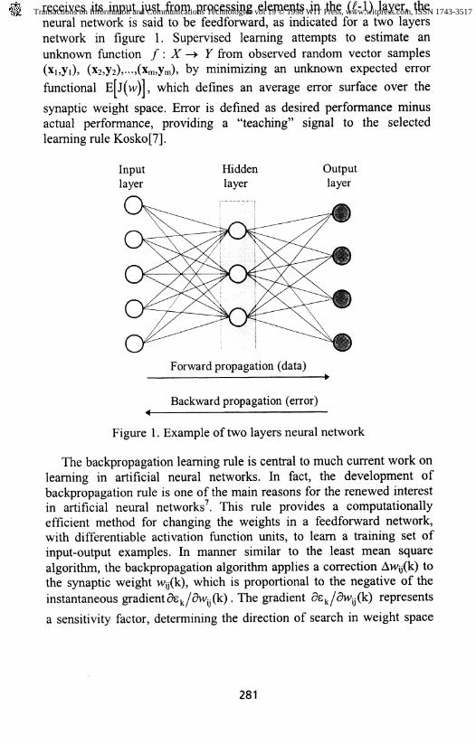
receives its input just from processing elements in the (&1) layer, theneural network is said to be feedforward, as indicated for a two layersnetwork in figure 1. Supervised learning attempts to estimate an

unknown function /: X -> Y from observed random vector samples(xi,y,), (X2,y2),..,(xm,ym), by minimizing an unknown expected error

functional E[j(w)l, which defines an average error surface over the

synaptic weight space. Error is defined as desired performance minusactual performance, providing a "teaching" signal to the selected

learning rule Kosko[7].

Hidden Outputlayer layer

Forward propagation (data)^

Backward propagation (error)4 •

Figure 1. Example of two layers neural network

The backpropagation learning rule is central to much current work onlearning in artificial neural networks. In fact, the development ofbackpropagation rule is one of the main reasons for the renewed interestin artificial neural networks . This rule provides a computationallyefficient method for changing the weights in a feedforward network,with differentiate activation function units, to learn a training set ofinput-output examples. In manner similar to the least mean squarealgorithm, the backpropagation algorithm applies a correction Awy(k) tothe synaptic weight Wy(k), which is proportional to the negative of the

instantaneous gradientd /dw (k) . The gradient de /Su k) represents

a sensitivity factor, determining the direction of search in weight space

281


for the synaptic weight Wy(k). The basic equation for error correction isthe following:

-i) (7)

where:

- Ck is the learning rate coefficient;

i is refered as momentun term

Figure 2 summarizes the computations needed to train a 2-layersfeedforward backpropagation neural network, that is also called Multi-Layer Perceptron neural network.

Data Feedforward

input elements: receive the input signal

Input -» hidden: multiply by weightshidden elements: sum the received signals

and apply activation function G

hidden -> output: multiply by weightsoutput elements : sum the received signals

and apply activation function G

_ U _

Error Backpropagation |

Uoutput elements: calculate errors

and multiply by derivative of activation function G

output -> hidden: sum the received signalsand calculate weight corrections

hidden elements: sum the received signalsand multiply by derivative of activation function G

hidden -» input: calculate the weight corrections

Apply Weight Corrections

Figure 2. Backpropagation technique summary

When building a neural network model, one of the most importantrequirements is that the model performs well on data that it has not seen

282


before. This property is refered to as generalization. The main reasons

why a model may not generalize well are:- the data selected to train the model may not be statistically

representative of the data population;- the model may be overfitting the data.

Sometimes the first reason is unavoidable, since the process that isbeing modeled may be changing statistically over the time andrepresentative data may not be available for training: this situationrepresents a nonstationary process.

The second reason can be overcome if a representative test set isavailable to evaluate the perfomance of the model as training isperformed. The error of the test set is monitored and the decision to stopthe training considers the tendency of this error.

Some constructive algorithms can also be applied to develop thehidden layers of the neural network model, which is the most sensitiveaspect of the neural network synthesis. The selection of the input datamay also be analyzed carefully.

3.2 Neural Networks on Updating

The concept of neural network can be applied for updating mass andstifness matrices according to the following equation:

8p=V,S;(s;VpS.+V,)~'8z=( Neural Net)8z (8)

where 5p, 5z, Sa, Vp and V% are already defined.The matrices Vp and V% will not be taken into account in this work, as

it is an initial development. The objective is simply the evaluation oflumped mass changes as a function of the variations in naturalfrequencies and natural modes of a spatial frame that represents themodel of a fixed offshore platform. The lumped masses, named mi, ni],ma and m*, are located at the upper corners of the spatial frame, asindicated at the figure 3. Variations in lumped masses are considered andtheirs respective natural frequencies and natural modes changes (first 3modes and frequencies) are calculated by finite element method. Thechanges in natural modes are calculated at the upper deck. Table 1indicates the natural frequencies variations.

Table 1 - Natural frequencies variations

Variable

frequency

mode 1

5f,

mode 2

5fj

mode 3

6fs

283


The first mode corresponds to vibration in tranversal direction, thesecond mode in longitudinal direction and the third one to the spatialframe torsion. The data regarding to the vibration modes are consideredat nodes 1 and 3 and for longitudinal and transversal directions. The

nodal displacement are named ty and £^, where the index i is referedto the vibration mode and the index j indicate the reference point and t

and i indicate the transversal and longitudinal directions. The dataprovided to the neural network are indicated in table 2.

Table 2 - Natural vibration modes variations

Variable

quotient 1

quotient 2

mode 1

S(t,., /*,,,)

5Ctu/*u)

mode 2

S(t2,l/*2.l)

8(t2,3/W

mode 3

6(t3.1/*3,l)

6(13,3/ ,3)

Model

longitudinal dir.

transversal dir.

Figure 3. Lumped mass location

The changes in mass for finite element calculation were providedaccording to table 3, where all the values are divided by mi .

284


Table 3 - Data refered to the lumped mass changes

mass changes

1

2

3

8m,

10%(m,)

20%(m,)

30%(m,)

8m2

10%(m,)

20%(mO

30%(m,)

8mj

15%(m,)

30%(m,)

45%(m,)

5ni4

15%(m,)

30%(m,)

45%(m,)

A number of 48 training vectors were prepared for neural networktraining. Each vector contains 9 values for the network input (3 naturalfrequencies and 6 modal displacements variations ) and 4 values for theneural network output (mass changes). For neural network test andevaluation, 14 test vectors were produced, with the same characterisesas the training vectors, using the modal analysis module of the FiniteElements Program ANSYSv5.0[X\.

The neural network topology is: 9 neurons at the input layer, 10neurons at two hidden layers and 4 neurons at the output layer. Thecriteria for training interruption is the non-convergence of test set. Theresults for the test set are presented in tables 4 and 5.

Table 4 - Data generated by FEM

Samples

1

2

3

4

5

6

7

8

9

10

11

12

13

14

8m i

7.00

15.00

-18.00

27.00

0.00

0.00

0.00

0.00

0.00

50.00

-50.00

0.00

0.00

0.00

Sm2

0.00

0.00

0.00

0.00

22.00

-25.00

0.00

0.00

0.00

0.00

0.00

-40.00

0.00

0.00

8rri3

0.00

0.00

18.00

0.00

0.00

0.00

-21.00

0.00

25.00

0.00

50.00

0.00

-59.00

0.00

5m4

0.00

0.00

0.00

-27.00

0.00

0.00

0.00

-35.00

-25.00

0.00

0.00

0.00

0.00

65.00

285


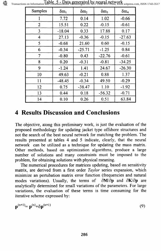
Table 5 - Data generated by neural network

Samples

1

2

3

4

5

6

7

8

9

10

11

12

13

14

8m,

7.72

15.51

-18.04

27.13

-0.68

-0.34

-0.80

0.20

-1.24

49.63

-48.45

0.75

0.44

0.10

5m2

0.14

0.22

0.33

-0.36

21.60

-25.71

0.43

-0.31

1.41

-0.21

-0.34

-38.47

0.18

0.26

Srtij

1.02

-0.15

17.88

-0.15

0.60

-1.25

-22.76

-0.81

24.67

0.88

49.50

1.10

-56.32

0.51

5ni4

-0.66

-0.61

l_ 0.17

-27.63

-0.15

0.84

-0.61

-34.25

-26.30

1.37

-0.29

-1.92

-0.71

63.84

4 Results Discussion and Conclusions

The objective, along this preliminary work, is just the evaluation of theproposed methodology for updating jacket type offshore structures andnot the search of the best neural network for matching the problem. Theresults presented at tables 4 and 5 indicate, clearly, that the neuralnetwork can be utilized as a technique for updating the mass matrix.Other methods, based on optimization algorithms, produce a largenumber of solutions and many constraints must be imposed to theproblem, for obtaining solutions with physical meaning.

The numerical procedures for matrices updating, based on sensitivitymatrix, are derived from a first order Taylor series expansion, whichminimize an pertubation matrix error function (frequencies and natural

modes variations). Usually, the terms of dM/dp and dK/dp areanalytically determined for small variations of the parameters. For largevariations, the evaluation of these terms is time consuming for theiterative scheme expressed by:

(9)

286


The neural network approach permits to simulate the terms of the

sensitivity matrices both for small and large parameters variations. Thedata for training is generated, for instance, by a computer program basedon finite element method.

References

[1] Mottershead, J. E. e Friswell, M. I., Model Updating in StructuralDynamics: a Survey, Journal of Sound and Vibration, vol. 167, no.2, pp. 347-375, 1993.

[2] Janter, T., Heylen, W. e Sas, P., QA Model Updating, Proceedingsof 14th International Seminar on Modal Analysis, Leuven, paper no.9, 1989.

[3] Natke, H. G., Updating Computational Models in the FrequencyDomain Based on Measured Data: a Survey, ProbabilisticEngineering Mechanics, vol. 3, no. 1, pp. 28-35, 1989.

[4] Hemez, F. M., Theoretical and Experimental Correlation BetweenFinite Element Nodels and Modal Tests in the Context of LargeFlexible Space Structures, Ph. D. Thesis, University of Colorado,

USA, 1993.

[5] Dascotte, E., Practical Applications of Finite Element Tuning UsingExperimental Modal Data, 8th. International Modal AnalysisConference, pp. 1032-1037, 1990.

[6] Lopes, T. A. P., Avalia$do do Dano de Fadiga em Plataformas dePetroleo em Tempo Real, Tese de D.Sc, COPPE/UFRJ, 1995.

[7] Kosko, B., Neural Networks and Fuzzy Systems: A DynamicalSystems Approach to Machine Intelligence, Prentice-HallInternational Editions, USA, 1990.

[8] Ansys (1992), ANSYS User's Manual - vol. I, II, III e IV, SwansonAnalysis Systems,inc., Houston, Texas, USA, 1992.

287


neural networks on the dynamic models - · pdf fileneural networks on the dynamic models...

Documents