1

Neural Networks(Part 1)

Mark Craven and David PageComputer Sciences 760

Spring 2018

www.biostat.wisc.edu/~craven/cs760/

Some of the slides in these lectures have been adapted/borrowed from materials developed by Tom Dietterich, Pedro Domingos, Tom Mitchell, David Page, and Jude Shavlik

Goals for the lectureyou should understand the following concepts

• perceptrons• the perceptron training rule• linear separability• hidden units• multilayer neural networks• gradient descent• stochastic (online) gradient descent• activation functions

• sigmoid, hyperbolic tangent, ReLU• objective (error, loss) functions

• squared error, cross entropy

2

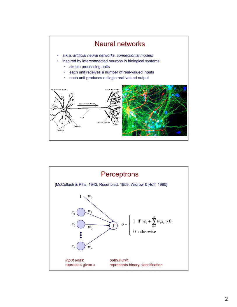
Neural networks• a.k.a. artificial neural networks, connectionist models• inspired by interconnected neurons in biological systems

• simple processing units• each unit receives a number of real-valued inputs• each unit produces a single real-valued output

Perceptrons[McCulloch & Pitts, 1943; Rosenblatt, 1959; Widrow & Hoff, 1960]

o = 1 if w0 + wii=1

n

∑ xi > 0

0 otherwise

"

#$

%$

input units:represent given x

output unit:represents binary classification

x1

x2

xn

w1

w2

wn

w01

3

Perceptron example

o = 1 if w0 + wii=1

n

∑ xi > 0

0 otherwise

"

#$

%$

x = 1,0, 0,1

x1

x2

x4

2.6

0.2

2.3

−51

x3 0.3

w0 + wii=1

n

∑ xi = −0.1 o = 0

x = 1,0,1,1 w0 + wii=1

n

∑ xi = 0.2 o =1

features, class labels are represented numerically

Learning a perceptron: the perceptron training rule

Δwi =η y − o( )xi

1. randomly initialize weights

2. iterate through training instances until convergence

o = 1 if w0 + wii=1

n

∑ xi > 0

0 otherwise

"

#$

%$

wi ←wi + Δwi

2a. calculate the output for the given instance

2b. update each weight

η is learning rate;set to value << 1

4

Representational power of perceptrons

o = 1 if w0 + wii=1

n

∑ xi > 0

0 otherwise

"

#$

%$

perceptrons can represent only linearly separable concepts

x1

+ ++ + +

+ -+ - -

+ ++ + -

+ + - --

+ + --

+ - - -

- -

x2

w1x1 +w2x2 = −w0

x2 = −w1w2

x1 −w0w2

1 if w0 +w1x1 +w2x2 > 0

decision boundary given by:

Representational power of perceptrons

• in previous example, feature space was 2D so decision boundary was a line

• in higher dimensions, decision boundary is a hyperplane

5

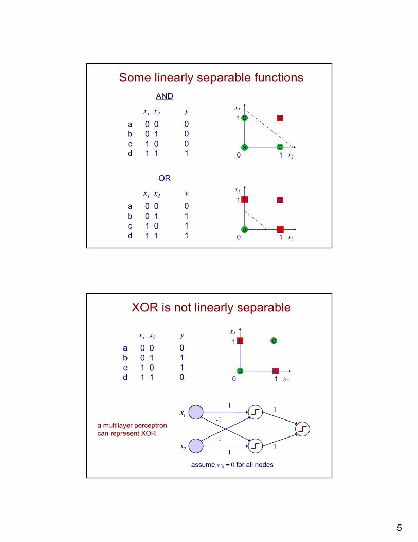
Some linearly separable functions

x1 x2

0 00 11 01 1

y0001

abcd

AND

a c0 1

1x1

x2

db

x1 x2

0 00 11 01 1

y0111

abcd

OR

b

a c0 1

1x1

x2

d

XOR is not linearly separable

x1 x2

0 00 11 01 1

y0110

abcd 0 1

1x1

x2

b

a c

d

x1

x2 1

-1

1

1

1-1

a multilayer perceptroncan represent XOR

assume w0 = 0 for all nodes

6

Example multilayer neural network

input: two features from spectral analysis of a spoken sound

output: vowel sound occurring in the context “h__d”

figure from Huang & Lippmann, NIPS 1988

input units

hidden units

output units

Decision regions of a multilayer neural network

input: two features from spectral analysis of a spoken sound

output: vowel sound occurring in the context “h__d”

figure from Huang & Lippmann, NIPS 1988

7

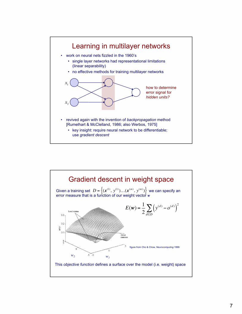
Learning in multilayer networks• work on neural nets fizzled in the 1960’s

• single layer networks had representational limitations (linear separability)

• no effective methods for training multilayer networks

• revived again with the invention of backpropagation method [Rumelhart & McClelland, 1986; also Werbos, 1975]• key insight: require neural network to be differentiable;

use gradient descent

x1

x2

how to determineerror signal for hidden units?

Gradient descent in weight space

figure from Cho & Chow, Neurocomputing 1999

E(w) = 12

y(d ) −o(d )( )2

d∈D∑

Given a training set we can specify an error measure that is a function of our weight vector w

This objective function defines a surface over the model (i.e. weight) space

w1w2

D = (x(1), y(1) )…(x(m ), y(m ) ){ }

8

Gradient descent in weight space

w1

w2

Error

on each iteration• current weights define a

point in this space• find direction in which

error surface descends most steeply

• take a step (i.e. update weights) in that direction

gradient descent is an iterative process aimed at finding a minimum in the error surface

Gradient descent in weight space

w1

w2

Error

−∂E∂w1

−∂E∂w2

∇E(w) = ∂E

∂w0

, ∂E∂w1

, !, ∂E∂wn

#

$%

&

'(

Δw = −η ∇E w( )

Δwi = −η ∂E∂wi

calculate the gradient of E:

take a step in the opposite direction

9

The sigmoid function• to be able to differentiate E with respect to wi , our network

must represent a continuous function• to do this, we can use sigmoid functions instead of

threshold functions in our hidden and output units

𝑓 𝑧 =1

1 + 𝑒'(

𝑧

The sigmoid functionfor the case of a single-layer network

𝑓 𝑛𝑒𝑡 =1

1 + 𝑒' +,-∑ +/�/ 1/

𝑛𝑒𝑡 = 𝑤3 +4 𝑤5�

5𝑥5

10

Batch neural network training

given: network structure and a training set

initialize all weights in w to small random numbers

until stopping criteria met do

initialize the errorfor each (x(d), y(d)) in the training set

input x(d) to the network and compute output o(d)

increment the error

calculate the gradient

update the weights

D = (x(1), y(1) )…(x(m ), y(m ) ){ }

E(w) = E(w)+ 12y(d ) − o(d )( )2

∇E(w) = ∂E

∂w0

, ∂E∂w1

, !, ∂E∂wn

#

$%

&

'(

Δw = −η ∇E w( )

E(w) = 0

Online vs. batch training

• Standard gradient descent (batch training): calculates error gradient for the entire training set, before taking a step in weight space

• Stochastic gradient descent (online training): calculates error gradient for a single instance (or a small set of instances, a “mini batch”), then takes a step in weight space– much faster convergence– less susceptible to local minima

11

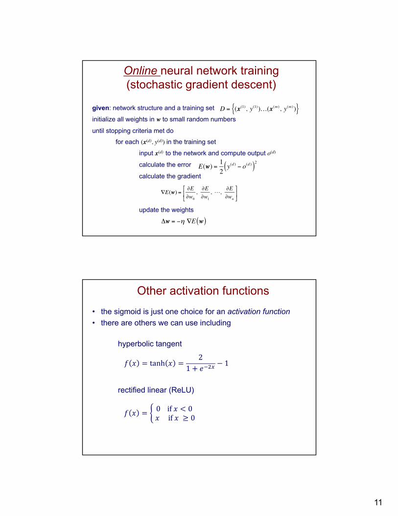
Online neural network training (stochastic gradient descent)

given: network structure and a training set

initialize all weights in w to small random numbers

until stopping criteria met dofor each (x(d), y(d)) in the training set

input x(d) to the network and compute output o(d)

calculate the error

calculate the gradient

update the weights

D = (x(1), y(1) )…(x(m ), y(m ) ){ }

E(w) = 12y(d ) − o(d )( )2

∇E(w) = ∂E

∂w0

, ∂E∂w1

, !, ∂E∂wn

#

$%

&

'(

Δw = −η ∇E w( )

Other activation functions• the sigmoid is just one choice for an activation function• there are others we can use including

𝑓 𝑥 = tanh 𝑥 =2

1 + 𝑒'<1 − 1

𝑓 𝑥 = > 0if𝑥 < 0𝑥if𝑥 ≥ 0

hyperbolic tangent

rectified linear (ReLU)

12

Other objective functions• squared error is just one choice for an objective function• there are others we can use including

𝐸 𝒘 = 4−𝑦 H ln 𝑜(H) − 1 − 𝑦 H ln 1 − 𝑜(H)�

H∈N

𝐸 𝒘 = −4 4 𝑦5(H)𝑙𝑛 𝑜5

(H)#QRSTTUT

5VW

�

H∈N

cross entropy

multiclass cross entropy

Convergence of gradient descent• gradient descent will converge to a minimum in the error function• for a multi-layer network, this may be a local minimum (i.e. there

may be a “better” solution elsewhere in weight space)

• for a single-layer network, this will be a global minimum (i.e. gradient descent will find the “best” solution)

• Recent analysis suggests that local minima are probably rare in high dimensions; saddle points are more of a challenge [Dauphin et al., NIPS 2014]