new analogues of clausen s identities arising from the …chanhh/papers/66.pdf · author's...

Author's personal copy

Advances in Mathematics 228 (2011) 1294–1314www.elsevier.com/locate/aim

New analogues of Clausen’s identities arising from thetheory of modular forms

Heng Huat Chan a,∗, Yoshio Tanigawa b, Yifan Yang c, Wadim Zudilin d

a Department of Mathematics, National University of Singapore, 2 Science Drive 2, Singapore 117543, Singaporeb Graduate School of Mathematics, Nagoya University, Nagoya 464-8602, Japan

c Department of Applied Mathematics, National Chiao Tung University, Hsinchu 300, Taiwand School of Mathematical and Physical Sciences, The University of Newcastle, Callaghan NSW 2308, Australia

Received 9 October 2010; accepted 7 June 2011

Available online 21 June 2011

Communicated by George E. Andrews

Dedicated to Professor B.C. Berndt on the occasion of his 73rd birthday

Abstract

Around 1828, T. Clausen discovered that the square of certain hypergeometric 2F1 function can beexpressed as a hypergeometric 3F2 function. Special cases of Clausen’s identities were later used by S. Ra-manujan in his derivation of 17 series for 1/π . Since then, there were several attempts to find new analoguesof Clausen’s identities with the hope to derive new classes of series for 1/π . Unfortunately, none weresuccessful. In this article, we will present three new analogues of Clausen’s identities. Their discovery ismotivated by the study of relations between modular forms of weight 2 and modular functions associatedwith modular groups of genus 0.© 2011 Elsevier Inc. All rights reserved.

Keywords: Clausen’s identities; Modular forms of one variable

* Corresponding author.E-mail addresses: [email protected] (H.H. Chan), [email protected] (Y. Tanigawa),

[email protected] (Y. Yang), [email protected] (W. Zudilin).

0001-8708/$ – see front matter © 2011 Elsevier Inc. All rights reserved.doi:10.1016/j.aim.2011.06.011


H.H. Chan et al. / Advances in Mathematics 228 (2011) 1294–1314 1295

1. Introduction

For |x| < 1, let

p+1Fp

(a0, a1, . . . , ap

b1, . . . , bp;x

)=

∞∑n=0

(a0)n(a1)n · · · (ap)n

(b1)n · · · (bp)n

xn

n! ,

where

(a)0 = 1 and (a)n = a(a + 1) · · · (a + n − 1) for n ∈ Z>0.

In his pioneering paper “Modular equations and approximations to π” [16], S. Ramanujanconstructed 17 series for 1/π and indicated briefly how he derived these series. In Section 13 ofthe paper, he cited a special case of Clausen’s identities [16, Eq. (25)], namely,

{2F1

( 12 , 1

21

;x)}2

= 3F2

( 12 , 1

2 , 12

1,1;4x(1 − x)

), (1.1)

and indicated its importance in the derivation of his series for 1/π such as

4

π=

∞∑n=0

(6n + 1)( 1

2 )3n

n!31

4n.

The complete proofs of Ramanujan’s series for 1/π , as well as many other generalizations,first appeared in the book “Pi and the AGM” [4] by J.M. Borwein and P.B. Borwein. Not surpris-ingly, Clausen’s identities are essential in Borweins’ proofs. Since then, several mathematicians(including some of us) have believed that in order to derive new classes of series for 1/π , newanalogues of Clausen’s identities are needed. Of course, this belief is not well reflected in theliterature (but see, for example, [3]), and it turns out to be incorrect. Around 2002, T. Sato [18]derived a series for 1/π associated with the Apéry numbers

An =n∑

k=0

(n

k

)2(n + k

k

)2

, n = 0,1,2, . . . . (1.2)

More precisely, Sato discovered that

1

π

√15

6(4√

5 − 9)=

∞∑n=0

(20n + 10 − 3√

5)An

(√5 − 1

2

)12n

. (1.3)

Sato’s series inspired H.H. Chan, S.H. Chan and Z.G. Liu [9] to construct Ramanujan-type seriesfor 1/π without the use of Clausen’s identities. Meanwhile, the search for new analogues ofClausen’s identities appears to have ceased.

In this article, we will present three new identities similar to Clausen’s identities associatedwith the Apéry-like integer sequences


1296 H.H. Chan et al. / Advances in Mathematics 228 (2011) 1294–1314

rn =n∑

k=0

(n

k

)3

, sn =n∑

k=0

(n

k

)2(2k

k

),

and tn =n∑

k=0

(n

k

)(−8)n−k

k∑j=0

(k

j

)3

. (1.4)

These are given by

{ ∞∑n=0

rnxn

}2

= 1

1 + 8x2

∞∑n=0

(2n

n

)rn

(x(1 + x)(1 − 8x)

(1 + 8x2)2

)n

, (1.5)

{ ∞∑n=0

snxn

}2

= 1

1 − 9x2

∞∑n=0

(2n

n

)sn

(x(1 − 9x)(1 − x)

(1 − 9x2)2

)n

, (1.6)

and

{ ∞∑n=0

tnxn

}2

= 1

1 − 72x2

∞∑n=0

(2n

n

)tn

(x(1 + 8x)(1 + 9x)

(1 − 72x2)2

)n

. (1.7)

It is clear that these identities are similar to (1.1) once we write (1.1) as

{ ∞∑n=0

( 12 )n(

12 )n

(1)n(1)nxn

}2

=∞∑

n=0

(2n

n

)( 1

2 )n(12 )n

(1)n(1)n

(x(1 − x)

)n. (1.8)

Our proofs of (1.5)–(1.7) will be given based on the study of modular forms associated withsubgroups of the normalizer of Γ0(6) in SL2(R).

The existence of new series for 1/π associated with the right-hand sides of (1.5)–(1.7) shouldnot be surprising since the search of new series for 1/π is the main motivation behind finding newanalogues of Clausen’s identities. We will list a new series for 1/π associated with the sequencesdiscussed in this article. Most of these series can be derived using ideas presented in [9] and westress again that their proofs are independent of the Clausen-type identities (1.5)–(1.7). Howeverthe same modular parametrizations are needed for proving both the series and identities. We endthis introduction with a preview of three of these new series for 1/π . These are

25

2π=

∞∑n=0

(9n + 2)

(2n

n

)rn

(1

50

)n

,

9√

3

2π=

∞∑n=0

(5n + 1)

(2n

n

)sn

(1

54

)n

,

and

8√3π

=∞∑

n=0

(10n + 3)

(2n

n

)tn

(1

64

)n

.



Note that there exists a different method for discovering and proving identities like (1.5)–(1.7),using computer algebra system such as MAPLE. We briefly outline this approach in Section 6together with further identities of this kind; more details on the method can be found in therecent work [1] by G. Almkvist, D. van Straten and W. Zudilin. A drawback of this algebraicmachinery is the lack of arithmetical insight; in particular, no series for 1/π can be obtainedusing this approach.

2. Some interesting binomial expressions and their relations with modular forms

We begin this section by describing the motivation behind our choices of modular forms andmodular functions that lead us to the discoveries of (1.5)–(1.7). We will then concentrate on thederivation of (1.5) and its related identities (such as the series for 1/π ). The derivations of (1.6)and (1.7) are similar.

We first fix some notations. Let N be a positive integer and let

Γ0(N) :={(

a b

c d

)∈ SL2(Z)

∣∣∣ c ≡ 0 (mod N)

}.

If e‖N , we call the matrix

We =(

a√

e b/√

e

cN/√

e d√

e

), a, b, c, d ∈ Z, det(We) = 1,

the Atkin–Lehner involution for Γ0(N). We let Γ0(N)+ to be the group generated by Γ0(N) andall the Atkin–Lehner involutions for Γ0(N). We will use Γ0(N)+e to denote the group generatedby Γ0(N) and We.

2.1. From binomial sums to modular forms

Our general approach is motivated by the following example. In light of Sato’s series (1.3)for 1/π , one may ask whether, for a given binomial expression analogous to (1.2), there exist1/π -series associated to it. As a test example, we consider the binomial expression

Bn =n∑

k=0

(n

k

)4

(2.1)

and its generating function

Z(X) =∞∑

n=0

BnXn.

Using the method of creative telescoping, one finds that Z(X) satisfies the differential equation

(1 − 12X − 64X2)θ3Z − (

18X + 192X2)θ2Z − (10X + 188X2)θZ − (

2X + 60X2)Z = 0,

(2.2)



where θ denotes the differential operator Xd/dX. We can verify that this differential equation isthe symmetric square of the differential equation

(1 − 12X − 64X2)θ2Y − (

6X + 64X2)θY − (X + 15X2)Y = 0. (2.3)

(That is, Z(X)1/2 is a solution of the latter second-order differential equation.) If its monodromygroup is a congruence subgroup of SL2(R), then there exists a modular form Z of weight 2 anda modular function X such that Z, as function of X, satisfies (2.2).

To determine the monodromy group of (2.3), one can employ the method of [11] to com-pute the monodromy group approximately and hopefully one can read off the group from thenumerical data. Here, however, the following indirect method works better.

Applying the Frobenius method to (2.2), we find a basis for the solution space near X = 0 isgiven by

F0(X) = 1 + 2X + 18X2 + 164X3 + 1810X4 + 21 252X5 + · · · ,F1(X) = F0(X)

(logX + g(X)

),

F2(X) = F0(X)

((logX)2

2+ g(X) logX + h(X)

),

where

g(X) = 4X + 30X2 + 760

3X3 + 2695X4 + 154 704

5X5 + · · · ,

h(X) = 8X2 + 120X3 + 4390

3X4 + 18 380X5 + 10 651 594

45X6 + · · · .

(Note that F0(X) is just Z(X).) Now if (2.2) is indeed the differential equation satisfied by amodular form F0(X(τ)) of weight 2 and a modular function X(τ), then we should have 2πiτ =F1(X)/F0(X) and

e2πiτ = eF1(X)/F0(X) = Xeg(X).

Setting q = e2πiτ = Xeg(X) and inverting the function, we get

X = q − 4q2 − 6q3 + 56q4 − 45q5 − 360q6 + 894q7 + 960q8 + · · · .

Substituting this into Z(X), we obtain

Z = 1 + 2q + 10q2 + 8q3 + 26q4 + 2q5 + 40q6 + 16q7 + 58q8 + · · · .

These should be the q-expansions of our hypothetical modular function and modular form. Toidentify what modular function X is, we observe that the orders of the local monodromy at thefour singularities 0, 1/16, −1/4, and ∞ are ∞, 2, 2, and 4, respectively. This means that X

should be a modular function on a congruence subgroup with one cusp, two elliptic points oforder 2, and one elliptic point of order 4. There are not many congruence subgroups of this



signature. In fact, the only congruence subgroup we can think of is Γ0(10)+. Indeed, after sometrial, we find that the function

{(η(τ)η(10τ)

η(2τ)η(5τ)

)6

+(

η(2τ)η(5τ)

η(τ )η(10τ)

)6

− 2

}−1

(2.4)

has the same starting q-expansion as X, while the modular form

1

12

(10P(10τ) + 5P(5τ) − P(τ) − 2P(2τ)

)(2.5)

has the same starting q-expansion as Z, where

η(τ) = q1/24∞∏

n=1

(1 − qn

)

is Dedekind’s eta function and

P(τ) = 12

πi

dη(τ)/dτ

η(τ)= 1 − 24

∞∑n=1

nqn

1 − qn

its (normalized) logarithmic derivative. We then use the method of [23] to verify that this pairof modular function and modular form indeed satisfies the differential equation (2.2). Now toobtain a series for 1/π analogous to Sato’s example (1.3), we may follow the procedure in [9].For example, we find

18√15π

=∞∑

n=0

(4n + 1)

n∑k=0

(n

k

)4 1

36n; (2.6)

here 1/36 is the value of X(τ) at τ = i/√

30.This example motivated us to search for other modular forms that are associated with elegant

binomial expressions such as (2.1). To do so, one can start with simple binomial expression andattempt to find suitable modular forms that are related to the expression. One can, on the otherhand, begin by studying various modular forms similar to the above example and hopefully derivebinomial expressions. We will adopt the latter approach in this article. Identities (1.5)–(1.7) arediscovered via this way.

Observe that the function in (2.4) is a Hauptmodul for Γ0(10)+ and the function in (2.5) is thelogarithmic derivative of

(η(5τ)η(10τ)

η(τ )η(2τ)

)2

,

which is a Hauptmodul for Γ0(10)+2. Thus, we introduce the following notations.Assume that Γ0(N)+m has genus 0 (see [5] for a complete list of such groups). Let XN,m

denote a fixed Hauptmodul for Γ0(N)+m. Corresponding to this Hauptmodul, we fix a modularform of weight 2 and denote this form by ZN,m. Next, we let



ZN,m = ϑ(ln(XN,m)

),

where

ϑ(F ) = qdF

dq= 1

2πi

dF

dτ.

Remark 2.1. Perhaps it would be more convenient to us to define ZN,m as Zϑ ln(XN,m), since

ZN,m is nothing else but ϑ ln(XN,m). We keep the easier notation in order to make many formulasbelow more accessible.

With this choice of ZN,m, we fix a modular function and denote it by XN,m. Throughout thepaper, we use the letter Z with subscripts for denoting modular forms of weight 2. With the abovenotation, the functions in (2.5) and (2.4) are written as Z10,2 and X10,2, respectively.

2.2. Binomial sums related to Γ0(6)+

A natural extension of the example above is to consider other subgroups of Γ0(10)+. We are,however, unable to derive sufficiently interesting results analogous to the example of Subsec-tion 2.1. As such, we turn our attention to Γ0(6)+.

We let

X6,2 =(

η(3τ)η(6τ)

η(τ )η(2τ)

)4

; (2.7)

this is our choice of a Hauptmodul for Γ0(6)+2. Its logarithmic derivative is

Z6,2 = 1

6

(6P(6τ) + 3P(3τ) − 2P(2τ) − P(τ)

). (2.8)

We next set

X6,2 = X6,6

(1 − X6,6)2, (2.9)

where

X6,6 =(

η(τ)η(6τ)

η(2τ)η(3τ)

)12

. (2.10)

Our first main result is

Theorem 2.1. For sufficiently small values of |X6,2|, we have

Z6,2 =∞∑

n=0

RnXn6,2 where Rn =

(2n

n

)rn =

(2n

n

) n∑k=0

(n

k

)3

. (2.11)



The discovery of (2.11) is coincidental. Using the q-series expansions of Z6,2 and X6,2, wecan first guess and then rigorously derive the recurrence satisfied by the sequence {Rn}, namely,

(n + 1)3Rn+1 + 2(2n + 1)(7n2 + 7n + 2

)Rn + 32n(2n + 1)(2n − 1)Rn−1 = 0. (2.12)

There is no efficient algorithm at present to determine Rn in terms of binomial expressionfrom (2.12). The only way, as D. Zeilberger pointed out several years ago to the first author,is to search for this sequence in databases such as [20] or [2]. If a binomial expression of oursequence shows up in the database, then we verify that our sequence has the given form in thedatabase by using creative telescoping (see [9,21,7] for such computations). If the sequence thatwe are interested does not appear in the database, then we are “out of luck”. Such is the case inour attempt to find Rn. In the following sketch of the proof of Theorem 2.1, we will only discussthe derivation of Rn.

Proof of Theorem 2.1. Using the theory of modular forms, we can show that if

Z6,6 = 1

24

(−5P(τ) + 2P(2τ) − 3P(3τ) + 30P(6τ)) = η7(3τ)η7(2τ)

η5(τ )η5(6τ), (2.13)

then

Z6,2 = Z6,6(1 − X6,6), (2.14)

where X6,6 is given by (2.10). It is known (see, for example, [7]) that

Z6,6 =∞∑

n=0

AnXn6,6 (2.15)

where the sequence {An} is the Apéry sequence (1.2). If we let Rn be such that

Z6,2 =∞∑

n=0

RnXn6,2,

then by (2.9), (2.15) and (2.14) we find that

∞∑k=0

Rk

Xk

(1 − X)2k+1=

∞∑n=0

AnXn (2.16)

where X = X6,6. Now, the left-hand side of (2.16) can be written as

∞∑k=0

∞∑m=0

(m + 2k

m

)RkX

m+k =∞∑

n=0

n∑k=0

(n

k

)(n + k

k

)Rk(2kk

)Xn. (2.17)

Comparing the coefficient of the resulting series in (2.17) with the corresponding one on theright-hand side of (2.16), we conclude that



n∑k=0

(n

k

)2(n + k

k

)2

=n∑

k=0

(n

k

)(n + k

k

)Rk(2kk

) . (2.18)

In order to determine Rk from (2.18) we recall that the Legendre transform of a sequence {ck}is the sequence

n∑k=0

(n

k

)(n + k

k

)ck.

V. Strehl [21] and A. Schmidt [19] proved independently that the Legendre transform of thesequence

rk =k∑

j=0

(k

j

)3

is the Apéry sequence (1.2), namely,

n∑k=0

(n

k

)2(n + k

k

)2

=n∑

k=0

(n

k

)(n + k

k

) k∑j=0

(k

j

)3

. (2.19)

Comparing (2.19) with (2.18) we conclude immediately that

Rk =(

2k

k

)rk =

(2k

k

) k∑j=0

(k

j

)3

. (2.20)

This completes the sketch of our proof. �2.3. Supercongruences

The following result shows that binomial expressions coming from differential equations sat-isfied by modular forms possess “strong” arithmetic properties.

Corollary 2.2. For prime p > 3, we have

Rnp ≡ Rn

(mod p3).

Proof. This follows immediately from the generalization [15]

(2np

np

)≡

(2n

n

) (mod p3)



of Wolstenholme’s theorem and [10, Theorem 4.2],

np∑k=0

(np

k

)3

≡n∑

k=0

(n

k

)3 (mod p3). �

Corollary 2.2 was motivated by S. Chowla, J. Cowles and M. Cowles [12]. They conjecturedthat for the Apéry numbers (1.2) and primes p > 3,

Ap ≡ A1(mod p3).

I. Gessel [14] proved this conjecture by showing that Anp ≡ An (mod p3). Recently, H.H. Chan,S. Cooper and F. Sica [10] showed that the Domb sequence {Dn}, defined by

Dn = (−1)nn∑

k=0

(n

k

)2(2k

k

)(2(n − k)

n − k

), (2.21)

satisfies the congruence Dnp ≡ Dn (mod p3). They also indicated a possible source of sequences{Fn} satisfying the congruence

Fnp ≡ Fn

(mod p3), (2.22)

and it turns out that {Rn} is one such example. It is therefore not surprising to see that Corol-lary 2.2 holds. However, the proof of Corollary 2.2 without the knowledge of the closed form ofRn is still missing.

The form Z6,2 and function X6,2 can also be written in terms of

Z6,3 = 1

6

(P(τ) − 4P(2τ) − 3P(3τ) + 12P(6τ)

) = η4(τ )η4(3τ)

η2(2τ)η2(6τ)(2.23)

and

X6,3 =(

η(2τ)η(6τ)

η(τ )η(3τ)

)6

. (2.24)

The analogues of (2.9) and (2.14) are then given by

X6,2 = X6,3

(1 + 8X6,3)2(2.25)

and

Z6,2 = Z6,3(1 + 8X6,3). (2.26)

It is known that (see [9,7] or [8])



Z6,3 =∞∑

n=0

DnXn6,3,

where Dn is given by (2.21). Using (2.26) and (2.20) we conclude that

(−1)nn∑

k=0

(n

k

)2(2k

k

)(2(n − k)

n − k

)=

n∑k=0

(n

k

)(n + k

k

)(−8)n−k

k∑j=0

(k

j

)3

. (2.27)

The interesting fact is that if we define

An(x) =n∑

k=0

(n

k

)(n + k

k

) k∑j=0

(k

j

)3

xn−k,

then (2.19) and (2.27) imply that {An(1)} gives the Apéry sequence (1.2) while {An(−8)} givesthe Domb sequence (2.21), and the two sequences satisfy the congruence (2.22). It does notappear that the sequences {An(N)} for integers N �= 1,−8 satisfy (2.22) (this was checked for amodest range of N ). We note that our function An(x) can be expressed as xna(1/x) where a(x)

is Schmidt’s function [19] defined by

a(x) =n∑

k=0

(n

k

)(n + k

k

) k∑j=0

(k

j

)3

xk.

It may be interesting to study functions similar to An(x). We end this section with the ob-servation that the Domb sequence and the Almkvist–Zudilin sequence (given in formula (3.2)below), a sequence that arises from Γ0(6)+2, can also be expressed as Bn(−16) and Cn(−27)

(see [8]), where

Bn(x) =n∑

k=0

(n

k

)(n + k

k

)(n + 2k

k

)(2k

k

)xn−k

and

Cn(x) =n∑

k=0

(n

k

)(n + k

k

)(n + 2k

k

)(n + 3k

k

)xn−k.

3. More identities arising from modular forms and functions on Γ0(6)+

In the previous section, we considered only the logarithmic derivative of X6,2. We first discussidentities associated with the logarithmic derivative of X6,3 defined by (2.24), followed by thoseassociated with the logarithmic derivative of X6,6 given in (2.10).

Theorem 3.1. Let

Z6,3 = 1

4

(6P(6τ) + 2P(2τ) − P(τ) − 3P(3τ)

)



and

X6,3 = X6,2

(1 + 9X6,2)2= X6,6

(1 + X6,6)2.

Then for sufficiently small |X6,3|,

Z6,3 =∞∑

n=0

SnXn6,3,

where

Sn =(

2n

n

) n∑k=0

(n

k

)2(2k

k

). (3.1)

In this case, the sequence {Sn} matches nicely with a sequence in [20]. We then verified thatthe binomial expression in the database is indeed Sn using the method illustrated in [9]. With theadditional identities

Z6,3 = Z6,6(1 + X6,6) = Z6,2(1 + 9X6,2)

and identities proved in [7], we derive the identities

n∑k=0

(n

k

)2(n + k

k

)2

=n∑

k=0

(n

k

)(n + k

k

)(−1)n−k

k∑j=0

(k

j

)2(2j

j

)

and

n∑k=0

(4k)!(k!)4

(n + 3k

4k

)(−27)n−k =

n∑k=0

(n

k

)(n + k

k

)(−9)n−k

k∑j=0

(k

j

)2(2j

j

). (3.2)

These are clearly analogues of (2.19) and (2.27).

Theorem 3.2. Let

Z6,6 = 1

2

(6P(6τ) + P(τ) − 2P(2τ) − 3P(3τ)

)and

X6,6 = X6,2

(1 − 9X6,2)2= X6,3

(1 − 8X6,3)2.



Then

Z6,6 =∞∑

n=0

TnXn6,6,

where

Tn =(

2n

n

) n∑k=0

(n

k

)(−8)n−k

k∑j=0

(k

j

)3

. (3.3)

The sequence {Tn} does not match with any sequence in [20]. However, motivated by theexpressions in (2.20) and (3.1), we consider the sequence tn = Tn/

(2nn

)that matches with Verrill’s

sequence [22]. Once again, using the method in [9], we verify that Tn is given by (3.3).Using the additional identities

Z6,6 = Z6,2(1 − 9X6,2) = Z6,3(1 − 8X6,3)

and the ones from [7], we derive the identities

(−1)nn∑

k=0

(n

k

)2(2k

k

)(2(n − k)

n − k

)=

n∑k=0

(n

k

)(n + k

k

)8n−k

k∑j=0

(k

j

)(−8)k−j

j∑i=0

(j

i

)3

and

n∑k=0

(4k)!(k!)4

(n + 3k

4k

)(−27)n−k =

n∑k=0

(n

k

)(n + k

k

)9n−k

k∑j=0

(k

j

)(−8)k−j

j∑i=0

(j

i

)3

.

These are again analogues of (2.19) and (2.27).

4. Proofs of the new analogues of Clausen’s identities

The motivation behind the derivations of (1.5)–(1.7) comes from the presence of the fac-tor

(2nn

)in (2.20), (3.1) and (3.3). In view of (1.8), one naturally expects identities similar to

Clausen’s identities to hold for sequences {Rn}, {Sn} and {Tn}.We now discuss the proof of (1.5). The proofs of (1.6) and (1.7) are similar.

Proof of (1.5). In [22], Verrill showed that if

z6,−2 = η6(3τ)η(2τ)

η2(τ )η3(6τ)(4.1)

and

X6,−2 = η3(τ )η9(6τ)

η3(2τ)η9(3τ), (4.2)



then

z6,−2 =∞∑

n=0

rnXn6,−2. (4.3)

(We use the small letter z for modular forms of weight 1.)Squaring (4.1) we find that

z26,−2 = Z6,6

η5(3τ)η(τ )

η5(2τ)η(6τ), (4.4)

where we have used the product representation of Z6,6 in (2.13). Now, we have

η5(3τ)η(τ )

η5(2τ)η(6τ)= 1

1 + X6,−2. (4.5)

Substituting (4.5) and (2.14) into (4.4) we conclude that

z26,−2 = Z6,2

(1 − X6,6)(1 + X6,−2). (4.6)

On the other hand, from [8] we find that

X6,6 = X6,−2(1 − 8X6,−2)

1 + X6,−2. (4.7)

The parametrization (4.7) allows us to conclude that

1 − X6,6 = 1 + 8X26,−2

1 + X6,−2(4.8)

and to write (2.9) as

X6,2 = X6,−2(1 + X6,−2)(1 − 8X6,−2)

(1 + 8X26,−2)

2. (4.9)

Substituting (4.8) and (4.9) into (4.6) and using (2.11) and (4.3) we conclude that for sufficientlysmall |x|, the identity (1.5) holds. �

The proofs of (1.6) and (1.7) are similar. In the case of (1.6) we use the fact (see [22]) that if

z6,−3 = η6(2τ)η(3τ)

η2(6τ)η3(τ )

and

X6,−3 = η4(τ )η8(6τ)

η4(3τ)η8(2τ),



then

z6,−3 =∞∑

n=0

snXn6,−3.

Then one applies several algebraic relations between X6,−3 and other modular functions such asX6,2; the details are left to the reader.

The proof of (1.7) requires the fact (see [22]) that if

z6,−6 = η6(τ )η(6τ)

η3(2τ)η2(3τ)

and

X6,−6 = η(2τ)η5(6τ)

η(3τ)η5(τ ),

then

z6,−6 =∞∑

n=0

tnXn6,−6.

Once again, the relations between X6,−6 and other modular functions such as X6,2 are needed.

5. Series for 1/π

As mentioned in the introduction, our discovery of the new analogues of Clausen-type identi-ties is motivated by numerical identities like (1.3) and (2.6). In [9], a general method is given toderive new classes of series for 1/π if one has the relation

Z =∞∑

k=0

anXn

for some modular form Z of weight 2 and modular function X and provided that Z satisfies acertain transformation formula. In this section, we will list the main identities and the “rational”series for 1/π associated with (Z,X) when

(Z,X) = (Z6,2, X6,2), (Z6,3, X6,3), and (Z6,6, X6,6).

By “rational” series for 1/π , we mean that C/π , for some algebraic number C, can be expressedas a series with rational terms. The integer N in the left column of the corresponding formulaindicates the degree of modular equation we use in the derivation of the series for 1/π . To proveeach series, one is required to derive a modular equation of degree N for the corresponding X.For more details the reader should consult [9].



5.1. Series associated with (1.5)

Let the sequence Rn be given by (2.20). The identities we need in order to prove the followingseries for 1/π are

qdX6,2

dq= Z6,2X6,2

√1 − 28X6,2 − 128X2

6,2

and

Z6,2(e−2π

√1/(6m)

) = mZ6,2(e−2π

√m/6).

For each value of N , we would also need a modular equation of degree N associated with X6,2.In these settings we have

N = 2: 25

2π=

∞∑n=0

(9n + 2)Rn

(1

50

)n

,

N = 3: 3√

2

π=

∞∑n=0

(5n + 1)Rn

(1

96

)n

,

N = 5: 8√

5√27π

=∞∑

n=0

(6n + 1)Rn

(1

320

)n

,

N = 7: 16√

7

π=

∞∑n=0

(90n + 13)Rn

(1

896

)n

,

N = 13: 50√

39

π=

∞∑n=0

(918n + 99)Rn

(1

10400

)n

,

N = 17: 1225√

6

π=

∞∑n=0

(10098n + 954)Rn

(1

39200

)n

.


Let the sequence Sn be given by (3.1). The identities we need in order to prove the followingseries for 1/π are

qdX6,3

dq= Z6,3X6,3

√1 − 40X6,3 + 144X2

6,3

and

Z6,3(e−2π

√1/(6m)

) = mZ6,3(e−2π

√m/6).

For each value of N , we would also need a modular equation of degree N associated with X6,3.



Then

N = 2: 9√

3

2π=

∞∑n=0

(5n + 1)Sn

(1

54

)n

,

N = 3: 25√3π

=∞∑

n=0

(16n + 3)Sn

(1

100

)n

,

N = 5: 37/2

π=

∞∑n=0

(80n + 13)Sn

(1

324

)n

,

N = 7: 75

29/2π=

∞∑n=0

(7n + 1)Sn

(1

900

)n

,

N = 13: 172√

6

25π=

∞∑n=0

(65n + 7)Sn

(1

10 404

)n

,

N = 17: 33 · 112 · √3

2π=

∞∑n=0

(9520n + 899)Sn

(1

39 204

)n

.


Finally, let the sequence Tn be given by (3.3). The required identities for the series below are

qdX6,6

dq= Z6,6X6,6

√1 + 68X6,6 + 1152X2

6,6

and

Z6,6(e−2π

√1/(6m)

) = −mZ6,6(e−2π

√m/6).

For each value of N , we would also need a modular equation of degree N associated with X6,6.Then

N = 3: 8√3π

=∞∑

n=0

(10n + 3)Tn

(1

64

)n

,

N = 5:√

6

π=

∞∑n=0

(5n + 1)Tn

(1

288

)n

,

N = 7: 18√

3

π=

∞∑n=0

(70n + 11)Tn

(1

864

)n

,

N = 13: 432√

3

π=

∞∑n=0

(2210n + 241)Tn

(1

10 368

)n

,



N = 17: 32√

51

π=

∞∑n=0

(770n + 73)Tn

(1

39 168

)n

.

6. Concluding remarks

Remark 6.1. In [6], while investigating Ramanujan’s cubic continued fraction, Chan andK.P. Loo attempted to derive a series for 1/π associated with the square of the series

∞∑n=0

n∑k=0

(n

k

)3

Gn,

with

G = G(q) = q1/3

1+ q + q2

1+ q2 + q4

1+ q3 + q6

1+ · · · .

The final result is

1

π= 3

√3(3 − 2

√2)

2

∞∑n=0

(n + 1 − 2

3

√2

) n∑k=0

{k∑

j=0

(k

j

)3 n−k∑i=0

(n − k

i

)3}(

3√

2 − 4

4

)n

.

We now know that the authors should have used the parametrization

G = G3 (1 + G3)(1 − 8G3)

(1 + 8G6)2. (6.1)

When q = e−2π/√

6, we have G = −1 + √6/2 and from (6.1), we find that G = 1/96. The

corresponding “correct” series should therefore be the second one (for N = 3) in Subsection 5.1.

Remark 6.2. The sequences

rn =n∑

k=0

(n

k

)3

and sn =n∑

k=0

(n

k

)2(2k

k

)

used in this article can be found in a manuscript written by D. Zagier more than ten years ago.This article is now published in [24].

Remark 6.3. The first series for 1/π associated with Sn = (2nn

)sn appears in M. Rogers’ work

[17, Eq. (3.12)]. The series,

2(64 + 29√

3)

π=

∞∑n=0

(520n + 159 − 48√

3)Sn

(80

√3 − 139

484

)n

,

was discovered as a consequence of his study of Mahler’s measure and a hypergeometric 5F4function.



Remark 6.4. Our choices of N are obtained directly from the tables in [7], where series for 1/π

corresponding to the Apéry numbers, the Domb numbers and the Almkvist–Zudilin numbers aregiven. With the exception of three “rational” series for 1/π , the series in [7] involve powers ofradicals in contrast with the ones given in Section 5.

Remark 6.5. There is another “uniform” way of proving identities (1.5)–(1.7) which avoids usingthe modular parametrizations and is in the spirit of the method given in [1]. The series

z(x) =∞∑

n=0

anxn

on the left-hand side of (1.5)–(1.7), where an is one of the sequences in (1.4), satisfy the second-order differential equation

(θ2 − x

(aθ2 + aθ + b

) + cx2(θ + 1)2)z = 0 where θ = xd

dx,

with

(a, b, c) = (7,2,−8), (10,3,9), and (−17,−6,72),

respectively (cf. [1]). This is equivalent to saying that

(n + 1)2an+1 − (an2 + an + b

)an + cn2an−1 = 0 for n = 0,1,2, . . . .

One can then show that

Z(x) =∞∑

n=0

(2n

n

)anx

n

satisfies the third-order differential equation

(θ3 − 2x(2θ + 1)

(aθ2 + aθ + b

) + 4cx2(θ + 1)(2θ + 1)(2θ + 3))Z = 0.

Finally, with the method given in [1], one finds that

z2(x) = 1

1 − cx2· Z

(x(1 − ax + cx2)

(1 − cx2)2

).

Applying the above idea to the remaining three cases of [1, Eq. (28)] with

(a, b, c) = (11,3,−1), (12,4,32), and (9,3,27),

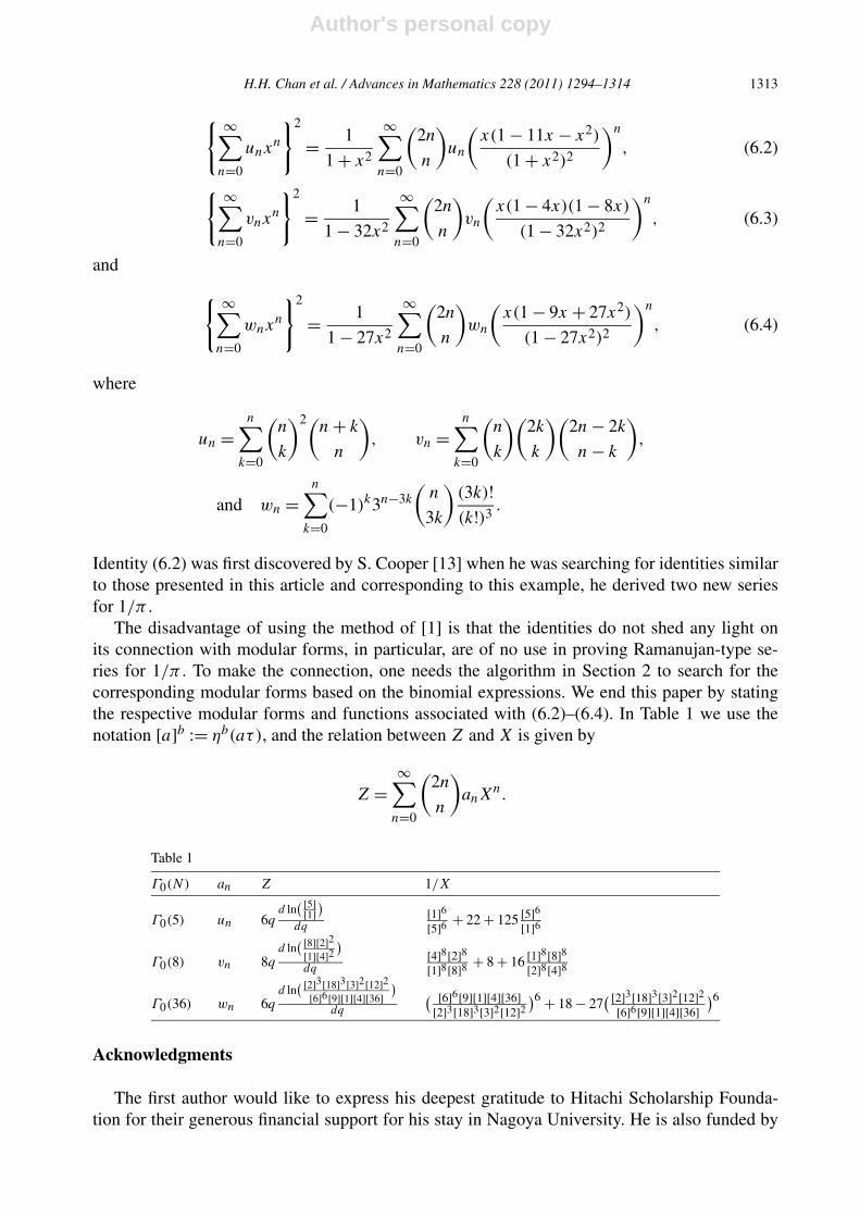
G. Almkvist and the fourth author (who also happens to be a coauthor of [1]) obtain three furtheranalogues of Clausen’s identities:



{ ∞∑n=0

unxn

}2

= 1

1 + x2

∞∑n=0

(2n

n

)un

(x(1 − 11x − x2)

(1 + x2)2

)n

, (6.2)

{ ∞∑n=0

vnxn

}2

= 1

1 − 32x2

∞∑n=0

(2n

n

)vn

(x(1 − 4x)(1 − 8x)

(1 − 32x2)2

)n

, (6.3)

and

{ ∞∑n=0

wnxn

}2

= 1

1 − 27x2

∞∑n=0

(2n

n

)wn

(x(1 − 9x + 27x2)

(1 − 27x2)2

)n

, (6.4)

where

un =n∑

k=0

(n

k

)2(n + k

n

), vn =

n∑k=0

(n

k

)(2k

k

)(2n − 2k

n − k

),

and wn =n∑

k=0

(−1)k3n−3k

(n

3k

)(3k)!(k!)3

.

Identity (6.2) was first discovered by S. Cooper [13] when he was searching for identities similarto those presented in this article and corresponding to this example, he derived two new seriesfor 1/π .

The disadvantage of using the method of [1] is that the identities do not shed any light onits connection with modular forms, in particular, are of no use in proving Ramanujan-type se-ries for 1/π . To make the connection, one needs the algorithm in Section 2 to search for thecorresponding modular forms based on the binomial expressions. We end this paper by statingthe respective modular forms and functions associated with (6.2)–(6.4). In Table 1 we use thenotation [a]b := ηb(aτ), and the relation between Z and X is given by

Z =∞∑

n=0

(2n

n

)anX

n.

Table 1

Γ0(N) an Z 1/X

Γ0(5) un 6qd ln

( [5][1]

)dq

[1]6[5]6 + 22 + 125 [5]6

[1]6

Γ0(8) vn 8qd ln

( [8][2]2[1][4]2

)dq

[4]8[2]8[1]8[8]8 + 8 + 16 [1]8[8]8

[2]8[4]8

Γ0(36) wn 6qd ln

( [2]3[18]3[3]2[12]2[6]6[9][1][4][36]

)dq

( [6]6[9][1][4][36][2]3[18]3[3]2[12]2

)6 + 18 − 27( [2]3[18]3[3]2[12]2

[6]6[9][1][4][36])6

Acknowledgments

The first author would like to express his deepest gratitude to Hitachi Scholarship Founda-tion for their generous financial support for his stay in Nagoya University. He is also funded by



NUS Academic Research Grant R-146-000-103-112. The work of the fourth author was sup-ported by a fellowship of the Max Planck Institute for Mathematics (Bonn) and by AustralianResearch Council grant DP110104419. We would like to thank Gert Almkvist for discussions onthe method from [1] which resulted in Remark 6.5. We are also very grateful to the referee forgiving suggestions which led to the present improved version of this work.

References

[1] G. Almkvist, D. van Straten, W. Zudilin, Generalizations of Clausen’s formula and algebraic transformations ofCalabi–Yau differential equations, Proc. Edinb. Math. Soc. 54 (2011) 273–295.

[2] G. Almkvist, C. van Enckevort, D. van Straten, W. Zudilin, Tables of Calabi–Yau equations, preprint, arXiv:math/0507430 [math.AG], 2005, 2010.

[3] R. Askey, Variants of Clausen’s formula for the square of a special 2F1, in: Number Theory and Related Topic, in:Tata Inst. Fund. Res. Stud. Math., vol. 12, Oxford University Press, Oxford, 1989, pp. 1–12.

[4] J.M. Borwein, P.B. Borwein, Pi and the AGM: A Study in Analytic Number Theory and Computational Complexity,Wiley, New York, 1987.

[5] H.H. Chan, M.L. Lang, Ramanujan’s modular equations and Atkin–Lehner involutions, Israel J. Math. 103 (1998)1–16.

[6] H.H. Chan, K.P. Loo, Ramanujan’s cubic continued fraction revisited, Acta Arith. 124 (4) (2007) 305–313.[7] H.H. Chan, H. Verrill, The Apéry numbers, the Almkvist–Zudilin numbers and new series for 1/π , Math. Res.

Lett. 16 (3) (2009) 405–420.[8] H.H. Chan, W. Zudilin, New representations for Apéry-like sequences, Mathematika 56 (2010) 107–117.[9] H.H. Chan, S.H. Chan, Z.G. Liu, Domb’s numbers and Ramanujan–Sato type series for 1/π , Adv. Math. 186 (2004)

396–410.[10] H.H. Chan, S. Cooper, F. Sica, Congruences satisfied by Apéry-like numbers, Int. J. Number Theory 6 (2010) 89–97.[11] Y.-H. Chen, Y. Yang, N. Yui, Monodromy of Picard–Fuchs differential equations for Calabi–Yau threefolds, J. Reine

Angew. Math. 616 (2008) 167–203.[12] S. Chowla, J. Cowles, M. Cowles, Congruences properties of Apéry numbers, J. Number Theory 12 (1980) 188–190.[13] S. Cooper, private communication, March 2009.[14] I. Gessel, Some congruences for the Apéry numbers, J. Number Theory 14 (1982) 362–368.[15] G.S. Kazandzidis, Congruences on the binomial coefficients, Bull. Soc. Math. Grèce (N.S.) 9 (1968) 1–12.[16] S. Ramanujan, Modular equations and approximations to π , Quart. J. Math. (Oxford) 45 (1914) 350–372.[17] M. Rogers, New 5F4 hypergeometric transformations, three-variable Mahler measures, and formulas for 1/π , Ra-

manujan J. 18 (2009) 327–340.[18] T. Sato, Apéry numbers and Ramanujan’s series for 1/π , Abstract of a talk presented at the annual meeting of the

Mathematical Society of Japan, 28–31 March 2002.[19] A.L. Schmidt, Legendre transforms and Apéry sequences, J. Austral. Math. Soc. (Ser. A) 58 (1995) 358–375.[20] N.J.A. Sloane, The on-line encyclopedia of integer sequences, published electronically at http://oeis.org, 2010.[21] V. Strehl, Binomial identities — combinatorial and algorithmic aspects, Discrete Math. 136 (1994) 309–346.[22] H.A. Verrill, Congruences related to modular forms, Int. J. Number Theory 6 (2010) 1367–1390, preprint MPIM

1999-26 (1999).[23] Y. Yang, On differential equations satisfied by modular forms, Math. Z. 246 (2004) 1–19.[24] D. Zagier, Integral solutions of Apéry-like recurrence equations, in: Groups and Symmetries: From Neolithic Scots

to John McKay, in: CRM Proc. Lecture Notes, vol. 47, Amer. Math. Soc., Providence, RI, 2009, pp. 349–366.

new analogues of clausen s identities arising from the …chanhh/papers/66.pdf · author's...

Documents