New Anthropomorphic Approaches to Global Warming:The Thermal Battery

Brett Teeple, Jode Himann1

a1018 72nd Ave NE, Calgary

Abstract

The role of anthropomorphic effects to global warming are examined and com-pared to the effects of greenhouse gases. It is shown that a significant reductionin temperature increases over the next decades can be ameliorated by a simplepower shutdown a few days at the temperate seasons around the globe, not justreducing CO2 emissions. The ’thermal battery’ needs only a couple days ofdischarge to reach climate change goals. Several models of climate change areinvestigated and mapped onto realistic parameters for the Earth and alternativesuggestions for resolving climate change are proposed. We predict that turningoff all power for even just a couple days every few months of the year removesthe anthropomorphic effect to global warming and allows time for a significantpercentage of the heat gain by CO2 increases to escape through the atmosphericwindow. Not everyone need turn their power off on the same day either and canrotate in shifts.

Keywords: Climate Physics Models, Global Warming, Thermodynamics,Electric Circuit Modelling, Warming, The Thermal Battery, Heat Pump,Emissivity Parameterization Suitable for Climate Modeling, climate physics,conduction, convection, radiation, climate science, fluid dynamics,thermodynamics, phase transformations of water, radiative-convective,equilibrium (RCE), troposphere, stratosphere, global warming, Newton’s lawof cooling, specific heat capacity, IPCC, Intergovernmental Panel on ClimateChange

Contents

1 Introduction 21.1 Outline of the paper . . . . . . . . . . . . . . . . . . . . . . . . . 2

2 The static case 5

1Since 1987.

3 The dynamic case 8

4 Climate change applications 11

5 Electric circuit equivalents of climate change and experimentalresults 20

6 The quantum case with discrete emission spectra 24

7 Conclusions 29

1. Introduction

Math and physics models are of great utility, as they give us a basis for rea-soning quantitatively about climate change. Despite this utility, however, manysuch models have not yet made it into the textbooks or popular literature, butremain scattered throughout the vast and technical scientific literature. Our aim5

here is to provide a self-contained treatment of a handful of these models whichseem particularly useful towards a total system model. The intended audienceare those with a math and physics background, and in particular scientists andengineers in other fields, who seek a basis for reasoning for themselves aboutclimate change. Although there exists many statistically based models of earths10

warming, there is very little on rigorous physics derivations of global warming.A novel method to model the atmospheric warming by developing a RC circuitare shown. A model of anthropomorphic heat piling in the atmosphere is devel-oped and investigated. Previous to these calculations, scientists have rejectedthe impact of our civilizations heat production here on earth. Compared to15

the sun human contribution only produce trace amounts of heat energy, leavingclimate scientists to dismiss waste kinetic heat as a cause of global warming.Thats true until you look at the case of heat piling as described below. In thecase of the Earth, we now think these anthropomorphic contributions and heatislands are much larger contributors to global warming that previously thought.20

From Newtons Laws of Cooling (and Heating), it follows that the time it takesto cool is longer than the time it takes to heat. It is found that the rate ofanthropomorphic heating is not in equilibrium with anthropomorphic cooling.The earths thermal setpoint is adjusting to compensate to the unequal rate ofchange in heating and cooling. We propose a cool down period of a day or two25

every few months to allow the earths anthropomorphic set point to stabilize.

1.1. Outline of the paper

Globally we use an enormous amount of energy, somewhere in the range ofabout 150 trillion kilowatt hours a year. We assume that 50% of this energy getsconverted to heat through inefficiency. This measurement only includes major30

measurable infrastructure. To get a sense of the relative scales involved, considerthe following: the total amount of energy delivered by the sun to the Earth isapproximately a million trillion (1018) kilowatt hours a year. So on the scale of

2

Figure 1: The Earth’s energy balance.

Figure 2: Global energy consumption and emissions [1]

what the Earth receives from the sun, our energy use represents only about 0.015percent of what is in principle actually available to us. Earth’s energy budget35

is vital in establishing the Earth’s climate. When the energy budget balances,the temperature on the Earth stays relatively constant, with no overall increaseor decrease in average temperature. However, not all of this energy reaches theEarth’s atmosphere or surface as some is reflected by clouds or the atmosphere.The energy that does pass through is absorbed by the atmosphere or the surface,40

and then moves around through convection, evaporation, or in the form of latent

3

Figure 3: Global temperature anomaly [2, 3].

Figure 4: Global temperature anomaly versus major volcanic eruptions releasing large amountsof atmospheric aerosols. The red blue diagram shows the temperature fluctuation near theequator at the Pacific Ocean showing the Ninos [2, 3].

heat. Today, the energy imbalance amounts to approximately 0.9Wm20.9Wm2of energy is coming in, than is leaving the Earth. The current suggestion is thathuman activities and a resultant increase in carbon dioxide is the major cause.

There exists many statistically based models of earths warming and there45

is very little on rigorous physics deriviations of global warming. It may seemlike an overwhelming task to model, with predictive accuracy, all the elementsof global warming. It is not as simple as calculating a perfect thermal sphere.

4

There are many variables and an almost impossible modelling of the system.This may be a reason that academics have relied heavily on experiment and50

statistics to draw their conclusions. To understand how a photon is emittingout into the vacuum of space and the dynamics of molecules requires a physicsmodel. Since the Earth is insulated in the vacuum of space, like a spacecraft,we cant eliminate heat without beaming it away. Unfortunately, the humanrace produces a significant amount of waste heat. Approximately, 50% of the55

energy from human activity is wasted as thermal kinetic energy or heat, throughelectrical infrastructure, internal combustion engines, camp fires and even bodyheat. With the elimination of this kinetic heat being extremely difficult, andthe production of kinetic heat at historical highs, we have a problem. Oncekinetic heat energy is created inside a system, the molecules and atoms move60

and vibrate in that system until the energy is converted to infrared radiation.Because this energy state change takes time, this leads to a significant temper-ature increase inside every closed system. In the case of the Earth, we nowthink it is the root cause of global warming (not greenhouse gases). As a simpleexample, the heat from your coffee cup will seemingly take 20 minutes to cool.65

We could calculate that the heat from your coffee and how it cools by infraredand kinetic energy then dispersion through the concrete and its specific heatcapacity. Then it would move up to the upper atmosphere and find the properoptical window for emission. This process takes about 18 hours (we calculate)and becomes a challenge if that heat piles by having a asymmetric heating and70

cooling rate.

2. The static case

Consider a globe being irradiated by the Sun. The spherical globe is coveredin a material/atmosphere that can reflect the light to prevent heating, but alsowith a certain blackbody constant (’greyness coefficient’ ε) so that the material75

may absorb and re-emit the solar radiation to cool down. Hence we have twodifferent thermal conductivities k1, k2, but the globe with anthropomorphic self-heating power P and initial inner surface temperature Ti, with incoming solarradiation on the blackbody surface of coefficient ε and reflectivity r of sometemperature To.80

In equilibrium. there must be no net heat flow across any isothermal surface,and so we have the following equalities at each of the boundaries:

−IA(1− r) +AεσT 4o = k1(To − T1)/t =

= k2(T1 − Ti)/d = P = PE +AEσT4i .

From here T1 can be found immediately in terms of To and Ti from themiddle equalities. The power P of the Earth’s heating is split into two parts,as it is not perfectly efficient as stated in the Introduction. Half its power goes85

to heat, as a blackbody spectrum at a certain temperature Ti. Plugging in thevalues for the solar irradiance given in the introduction, and taking To → 0 for

5

the vacuum of space (this can’t always be assumed as we will see in a futurecase where I consider a layer that is heated near the surface in space), we canfind the shift in the blackbody spectrum.90

Let us now look at two more examples, and increase the detail of the problemto look at global warming.

A first example is simply how long does it take a jacuzzi to cool? Or say,for simplicity, how long does it take a spherical blackbody at temperature T0 tocool to temperature Th in an environment of ambient temperature Ta?95

First, let us assume that we can ignore thermal conductivity. This can be as-sumed when, for example, the blackbody is in no atmosphere, or its temperatureis sufficiently high throughout much of the cooling process. One can show thatthis holds specifically for T >≈ 3.16Ta by computing conduction and cooling co-efficients, and solving for T . For Earth with an ambient temperature of 300 K,100

this corresponds to T > 1000 K for pure radiators, so certainly conduction mustbe included in examining global warming, as well as the jacuzzi. Sticking to thecase of the hot blackbody, we can also ignore the ambient temperature up to1% errors. This case is pure radiative cooling, and

P =dE

dt= εσA(Thot(t)

4 − T 4a ).

It does not matter what material the blackbody is made out of, though we105

assume it has a very large thermal conductivity, so that all heat inside thebody reaches the surface infinitely fast to be radiated away when needed. Let’sassume all the heat in the blackbody is attributed to translational degrees offreedom only, as kinetic energy, and by the law of equipartition E = 3

2NkbT ,where N = mNA/Mmolar is the number of particles in the blackbody of mass110

m. Therefore,

dE

dt=dE

dT

dT

dt=

3

2Nkb

dT

dt= εσAT (t)4,

(in our approximations above). This is a separable differential equation giving

tcool =

∫ t

0

dt =

∫ Tf

T0

3Nkb2σεAT 4

dT =Nkb2εσA

[1/T 3f − 1/T 3

0 ].

Again, because materials do not have infinite thermal conductivities, thisgives a lower bound on the cooling time for the blackbody, as the inside of theblackbody will take time to reach the surface and radiate away. This exam-115

ple also ignores convection, which is okay in purely radiative cases, but whenconduction comes into play, when convection exists, the thermal conductivitychanges with temperature during those temperature ranges.

Considering also an external heat source, like the Sun, we can computeheating times...120

I mentioned above the case where there is an atmospheric shell (we canmodel the edge of Earth’s atmosphere as a blackbody on one side as there isno conduction of heat into space, only radiation, but let’s simplify it further for

6

now...). How this affects the problem is purely geometrical as I state in thistheorem:125

Theorem) A spherical blackbody of radius r = REarth at temperature T issurrounded by a thin atmospheric shell of radius R, treated as a blackbody onboth sides. The factor by which this ’atmosphere’ reduces the cooling of theEarth is given by R2/(r2 +R2).

Proof:130

For an internal ’atmosphere’ of temperature T0, the rate of heat loss beforethe shell is placed is

Q = 4πr2σ(T 4 − T 40 ),

and after the atmospheric shell is added is

Q′ = 4πr2σ(T 4 − T 41 ),

where T1 is the temperature of the shell. The power loss by the shell is

Q′′ = 4πR2σ(T 41 − T 4

0 ).

By conservation of energy, Q′ = Q′′ and so

T 41 =

r2T 4 +R2T 40

R2 + r2

and so thus

Q′/Q = R2/(R2 + r2).

Now the case of pure conduction is given by Newton’s law of cooling, and135

is more simple. Since, as above, Q ∝ T , we have the law of conduction and itssolution:

dT

dt= −h(T − T0) → T (t) = Ta + (T0 − Ta)e−ht,

where h is related to the usual thermal conductivity k by h = 2Ak/3Nkb (againassuming translational thermal kinetic energies only). Heat conductivities rangefrom k ≈ 10−2− 103 W/m K from snow to diamond respectively. Inverting the140

solution to the differential equation above gives a conductive cooling time of

tcool =1

hlnT0 − TaTf − Ta

.

The case when both conductive and radiative heat transfers are significantwe have the general equation

dT/dt = h(T − Te) + σ(T 4e − T 4)

This differential equation is separable with general solution found by solvingthe integral using simple complex analysis and application of Cauchy’s integral145

formula:

7

t =

∫ Tf

T0

dT

a− bT − σT 4=

∑ω:bω/a−σω4/a−1=0

log(T − ω)

a− 4bω3|Tf

T0

, here b = σ/h and a = σT 4e − hTe. The only hard part is solving the quartic

polynomial, which can be done numerically. It has no imaginary part in mostcases of physical significance.

In cases where the ambient temperature, or T0 can be ignored, the solution150

is simple:

t =

∫dT

−T + bT 4=

1

3(T−3 − b) + C,

for t > 0, T > Te, or the environment temperature, and b > 0. This equationcan be inverted to solve for the temperature curve as a function of time:

T (t) = (e2hAt/Nkb−C + σ/h)−1/3.

Now T (0) = T0, so we solve for the integration constant C = − log(T−30 −σ/h), and plugging it in, the result simplifies once again to a Newton’s cooling155

curve when ambient temperature can be ignored, but with but conduction andradiation present:

T (t) = T0e−2hAt/3Nkb !!

In the case of pure radiative cooling, we have instead:

Q = mcT (t) = εσ(T 4e − T 4(t)),

which is a separable differential equation which integrates (by either Cauchy’sintegral theorem or by partial fractions) to give the cooling time from Ti to Tf160

to be

tcool =mc

εσ

∫ Tf

T0

dT

T 4e − T 4

=mc

4εσT 30

[ln(Te + T )− ln(Te − T ) + 2 tan−1T

Te]|Tf

T0.

3. The dynamic case

Consider a spherical light source being heated by conduction by solar radi-ation of power P . The conservation of energy implies for r < R

−4πr2kdT

dr= P

4

3πr3,

which integrates to give the temperature difference to the inner boundary at R:165

∆T (r) = −Pr2

6k+ C,

for some constant C to be determined.

8

For r > R conservation of energy now means that

−4πr2kdT

dr= P

4

3πR3.

This integrates now to

∆T (r) = PR3/3kr,

where there is no constant this time, as for r →∞ there is no heating. Equatingthe two solutions at r = R gives C = PR2/2k, which shows the new temperatureat the LED surface (r=0) is now

T ′i = Ti + PR2/2k!

This shifts its blackbody spectrum.In the case where the surface at r = R radiates as a blackbody as in the

previous section we can continue the analysis as above and obtain a result in170

terms of the coefficient ε of the coating as well! Let us proceed...For the case of looking over time we must look at the heat equation, which

can be derived from the simple conductance equation for heat q = −k∇T .

T =k

cpρ∆T.

The constant α = kcpρ

is called the thermal diffusivity. Now radiative corrections

also have a role and for small and large excess temperatures the heat equation175

must be adapted to, respectively:

T =k

cpρ∆T − µT or T =

k

cpρ∆T −mT 4,

where m = εσp/ρAcp. These equations are simply solved using Fourier seriestypically.

By separation of variables and using superposition, the general solution forthe temperature in the slab (representing a local part of Earth) is, supposing it180

has constant initial temperature Ti and then is suddenly bombarded with solarradiation of intensity I,

T (x, t) =

∞∑n=1

bn sin(nπx)e−n2π2t + Tf ,

where x is the direction pointing into the slab towards the LED (normalizedso = distance/thickness), and the Fourier coefficients are given from the initialtemperature distribution:185

bn = 2

∫ 1

0

sin(nπx)Tidx = 4Ti/nπ, 0,

for n odd and even respectively. The solution then becomes

9

T (x, t) =4Tiπ

∞∑n=1

sin(2n− 1)πx

2n− 1exp(−(2n− 1)2π2t)

≈ 4Tiπ

(sinπxe−π2t +

sin(3πx)

3e−9π

2t + · · · ).

Notice that the second term is less than 0.00034 times the first term fort > 1/π2, which corresponds to a physical (non dimensionless) time of t′ = l2t/kwhich is about 15 minutes for 1m of copper (k = 1.1 cm2/s), 169 minutes for1m of steel (k = 0.1 cm2/s) or 47 hours for 1m of glass (k = 0.006 cm2/s).190

At t = 1/π2, the temperature at the centre of the slab (note: I made this asymmetric problem so it is mirror imaged) is

T (1/2, 1/π2) ≈ 4Ti/πe+ Tf = 0.47Ti + Tf .

Note that the temperature exponentially reaches its steady state and neverattains it exactly. Tf depends on what was calculated above and depends onthe solar irradiance I. The initial condition is easily adapted to from the casehere of cooling from Ti to 0, to the case of heating from Ti to Tf . The sameprincipal applies, the same time constants appear, and the same graphs and195

plots result. Plots of temperature over space are sine arcs and over time areexponential decays.

This can be extended to sources and radiation as well, and the Fourier seriessolution can be modified. Let me solve the partial differential equation fully thistime in the quasi 1D geometry introduced originally. The heat equation and its200

initial and boundary conditions read (writing now the temperature as u(x, t)and the conditions are different but can be arranged with a different mirrorsymmetry):

∂tu = k∂xxu− µu,

u(x, 0) = f(x), ∀x ∈ [0, `]

u(0, t) = 0 = u(`, t),∀t > 0.

By the method of separation of variables we assumes that the temperaturefunction can be split into a product of functions that depend on just time and205

space: u(x, t) = X(x)T (t), which when substituted into the original partialdifferential equation, gives:

XT ′ = kTX ′′ − µXT → T ′/kT = X ′′/X − µ = −λ,

where λ is a chosen constant as both sides of the latter equation depends ondifferent variables x and t, and so both sides must be a constant. We then areleft with two linear ordinary differential equations:210

10

T ′ = −λkT (t)

X ′′ = −(λ− µ)X(x).

It can be shown that λ′ = λ− µ > 0. Else if λ′ < 0 Then

∃B,C ∈ R : X(x) = Be√−λ′x + Ce−

√−λ′x,

but X(0) = 0 = X(`) implies B = C = 0. And if λ′ = 0, then X(x) = Bx+ Cwhich by the boundary conditions also implies that B = C = 0. When λ′ > 0we have solution:

T (t) = Ae−λkt

X(x) = B sin√λ′x+ C cos

√λ′x.

With the boundary conditions this means that C = 0 and that√λ′ = nπ/`

for any n ∈ N. By linear superposition of solutions, we get the Fourier series215

solution combined:

u(x, t) =

∞∑n=1

Bn sinnπx

`e−(n

2π2/`2−µ)kt,

where the Fourier coefficients are easily found by orthogonality

Bn =2

`

∫ `

0

f(x) sinnπx

`dx.

Note that this decreases the characteristic 1/e heating time for the LED bythe µ term to now a time constant of

τ ′ = `2/π2k − 1/µk.

One can numerically do further considerations with the quartic radiativeequation, but this is only for very high temperature gradients, but can be aproblem if wanted in future investigation. Some analytic studies are done in [4].220

4. Climate change applications

Given the complexity of the climate system, the simplifications required tomake our models tractable will be drastic at times. In this sense we will ’lie totell the truth’, but we will endeavor to make our lies explicit, pointing out whereapproximations are made and where further work is needed. We will often focus225

on the Earth’s tropics, sometimes treating it as a stand-in for the entire planet.This is justified to some degree as the tropics account for half the Earth’s surfaceand the majority of it its incoming and outgoing radiation and precipitation.

11

We will also focus on the vertical transports of energy and moisture, and ignorehorizontal transports; the latter are crucial for determining the atmospheric230

circulation and meridional temperature gradients, but the former is perhapsmost crucial for determining climate overall, and in particular for determiningthe surface temperature Ts, the central variable in climate science. Indeed,much of the field is focused on understanding how Ts responds to forcing, andhow forcing-induced changes in Ts affect other variables such as precipitation,235

clouds, or humidity. We thus begin by considering the present day, global andannual mean Ts of 288 K. Where does this number come from?

This is a good first question to start at. To find the Earth’s temperature westart with sunlight, as mentioned in our Introduction. It has a solar intensityat Earth of I0 = 1360 W/m2, incident on an effective surface area of πR2

E .A fraction of this light α, called Earth’s albedo, is reflected back into space.Dividing by Earth’s total surface area, 4πR2

E , we then get the total incomingsolar radiation at Earth’s surface to be

Is = I0(1− α)πR2E/4πR

2E ≈ 240 W/m2.

Note that this is averaged over day and night and over the latitude angle.This is the energy absorbed by the Earth and is not to be confused with thearound 1050 + W/m2 of solar intensity that reaches Earth’s surface. Now for240

energy balance in equilibrium, the ’outgoing longwave/IR radiation’ (OLR) asmentioned in the Introduction, must balance this incoming solar radiation:

Is = OLR = σT 4em.

This predicts Tem = 255 K, which is much smaller than our to-date Ts =288 K, but is a reasonable estimate of vertically averages atmospheric temper-atures and not surface temperatures, as makes sense as OLR is mainly released245

from CO2 and H2O greenhouse gases in the atmosphere. Now given Tem howcan we find Ts? More physics is necessary!

The extra physics required is shown in Figure 2. The idea is of radiative-convective equilibrium (RCE). The part of the atmosphere where RCE me-diation is by convection is the troposphere, occupying the bottom 15 km of250

the atmosphere in the tropics, and roughly 9/10 of the atmosphere’s mass andpressures around 0.1 atm. Above the troposphere is the stratosphere, whichis heated mainly by UV solar absorption and is in pure radiative equilibriuminstead of RCE. Let us consider the troposphere first.

The troposphere contains pockets of air that rise by convection and cool at255

a rate of 7 K/km, which one can derive using the ideal gas law and ∇p = −ρ~g,and assume an adiabatic process. This is also similar to the temperature profileof the troposphere. We see this as by the first law of thermodynamics and theideal gas law (and dQ = 0 for an adiabat, and U = ρV cvT ),

dQ = 0 = dU + pdV, p = ρRT, dp/dz = −ρg

→ 0 = ρCpdT − dp, → Γ ≡ −dTdz

= −g/cp ≈ 10 K/km,

12

where as usual cp = cV + R = 1000 J/kg/K was used to approximate the260

change in temperature with height.Now let us see how convection can determine the actual Ts we observe today.

From a linear relation we derived for parcels of air in the troposphere, we havethe actual atmosphere temperature profile compared to the average temperatureof the OLR, say at a height of 5 km, giving:265

Ts = Tem + Γmzem ≈ 290 K,

where Γm is the temperature loss rate for a cooling parcel of moist air at averageheight, and zem is the emission height at the average troposphere height, wherethe emission pressure is average and thus at 0.5 atm. A calculation then giveszem ≈ 5 km, yielding the result for Ts above, which is quite close to the observedTs = 288 K today. Now we can look at what can cause equilibrium to change,270

and hence global warming and climate change.To look now at the anomaly of surface temperature increase over a doubling

of greenhouse gases or of heating due to human impact, we look to the oceans.Global climate model calculations [4] show that a doubling of CO2 in the at-mosphere instantaneously decreases the OLR by F2x ≈ 3.6 W/m2, which here275

can be thought of as an increase instantaneously in zem, lowering Tem which isconsistent with the lowering of the OLR. This puts the planetary energy balanceoff and causes energy to accumulate in the system. Figure 3 shows a model ofhow the oceans will respond.

Figure 5: How the decrease in OLR heats the top mixed layer of the oceans and heats as wellthe Ts of the Earth’s surface. [4]

This decrease in OLR predicts four things: (1) a decrease in precipitation280

(as condensation heating balances the radiative emission from the troposphere),(2) the boundary layer above the ocean surface moistens (as the rate at whichboundary layer moisture is converted to precipitation has decreased), (3) evap-oration has decreased (as it is limited by the vapour pressure of the increased

13

boundary layer humidity), and (4) Ts increases (because evaporation is how the285

ocean cools itself, and the ocean is 2/3 the Earth’s surface).What are the timescales for these processes? For atmospheric processes like

boundary layer moistening it is about 1 day, but what about Ts? To answerthis, look at the ocean with a mixed layer of about a depth of hml ≈ 100 m anda deep ocean layer beneath it of average depth hd ≈ 3000 m. The mixed layer290

will warm due to the decreased evaporation and develop a uniform temperatureanomaly T ′ml, which is also the Ts anomaly. This will spread to the net topatmosphere radiation OLR−I, which linearized becomes βT ′ml, where the slopeis

β ≡ dOLR

dTs− dI

dTs.

The derivatives are taken at the fixed doubled C)2 concentration and say how295

much Ts must increase until the OLR is back in balance with I. The T ′mlanomaly will also export heat to the deep ocean by conduction, which can belinearized by γ(T ′ml−T ′d). Typical values from global climate models have foundβ ≈ γ ≈ 1 W/m2/K. We can estimate β to an order of magnitude by ignoringthe small value of dI/dTs (as we will in the experiment and RC model in the300

next Section), and get the estimate

βblackbody =dOLR

dTem

dTemdTs

= 4σT 3em ≈ 3.5 W/m2/K.

This is still a significant over estimate for now. For γ, there do not seem to beany simple models, even for an order of magnitude estimate yet.

Now, using the density and heat capacities of the oceans, we then have thefollowing conduction equations linearized:305

ρwcwhmlT′ml = F2x − βT ′ml − γ(T ′ml − T ′d),

ρwcwhdT′d = γ(T ′ml − T ′d).

The larger depth and heat capacity of the deep ocean suggests it will takemuch longer to respond to the greenhouse gas F2x forcing than the mixed layer.From the differential equations above, we can find the respective timescales.First, if we assume the deep ocean hasn’t responded yet, that is its anomaly iszero, T ′d = 0, then the first equation gives a timescale310

τml =ρwhmlcwγ + β

≈ 6 years.

Now if we take timescales longer than τml, we can set its change in anomaly tozero, dT ′ml/dt = 0, solve for T ′ml, plug it into the second differential equation,and get a characteristic timescale for the deep ocean of

τd = ρwhdcwγ + β

γβ≈ 600 years.

14

The main difference is due to the larger heat capacity of the deep ocean.On timescales intermediate between τml and τd, the mixed layer is in quasi-equilibrium and we can assume that dT ′ml/dt = 0 and T ′d ≈ 0, which the firstequation above then gives

T ′ml =F2x

γ + β≈ 1.8 K.

This is called the transient climate response, before the deep ocean has re-sponded. This is to be compared to the equilibrium climate sensitivity, which is315

the surface warming after both the mixed layer and the deep ocean have reachedequilibrium (T ′ml = 0 = T ′d), after hundreds of years. In this two box model, wesolve to get

T ′d = F2x/β ≈ 3.6 K,

which can model the global warming temperature increase to Ts over hundredsof years. However, this simple radiative convection model gave a value of β ≈320

3.5 W/m2/K, which is almost 4 times higher than the research quoted value of1 W/m2/K, so we must look into more detail.

But first, let’s do some math examples of other problems.One significant mechanism of radiative-convective cooling in the Earth is the

Hadley cycle. Figure x shows Earth’s tropical atmosphere around the spring325

equinox where warm air rises at the equator and drops at latitudes ±φd in thesubtropics. The angular momentum about the Earth’s spin axis is conservedfor the upper branches of the circulation. From this angular momentum con-servation we can find the east-west wind velocity at the points Y:

ΩR2 = (ΩR cosφd + uY )R cosφd, → uY = ΩR(1/ cosφd − cosφd),

where R is the radius of the Earth, and Ω is its angular velocity.330

(Angular momentum is not conserved in the lower branches of the Hadleycirculation mainly because of turbulence in the lower atmosphere where differentlayers of air are mixed, and there is friction from the Earth’s surface.)

During the northern winter solstice the rising branch of the Hadley circula-tion occurs at latitude φr and drops at latitudes φR and φS . Conservation of335

angular momentum about the Earth’s spin axis again gives the wind speed u atlatitude φ:

ΩR2 cos2 φr = (ΩR cosφ+ u)R cosφ, → u = ΩR(cos2 φr/ cosφ− cosφ),

and a direct calculation shows that the winter hemisphere has a stronger atmo-spheric jet stream (for example, with φr = −8, φR = 28, φS = −20, we getu = 105 m/s at the North, u = −8.97 m/s at the equator, and u = 48.1 m/s at340

the South end). Note that there is also a westward Coriolis force on the tropicalair mass north of the equator and eastward south of the equator.

15

Figure 6: Hadley circulation.

Figure x now shows the Hadley cycle as a heat engine. It can be simplyargued that pE > pA > pD > pB > pC , and if we are given that the pressuredifference between points A and E is 20 hPa, the temperature at the top of345

the circulation TC can be found in terms of that at the bottom TH assumingadiabaticity with R/cP = 2/7:

p−R/cPE TH = p

−R/cPD TC ,

which gives TC = 195 K for pA = 1000 hPa and TH = 300 K. The pressure pBis found from the adiabatic expansion AB and adiabatic compression DE,

p−R/cPA TH = p

−R/cPB TC , p

−R/cPE TH = p

−R/cPD TC , →

pB = pApD/pE = 220 hPa.

The work done in isothermal processes EA and BCD are350

16

Figure 7: Hadley cycle.

WEA =

∫pdV = RTH ln pE/pA, WBCD = RTC ln pB/pD.

The work done in the adiabatic processes raises the internal energy of the airmass. Since the internal energy increase in process DE is exactly lost in processAB as the temperature returns to the same value, no net work is done is theadiabatic processes. Thus the total net work of the process is

ΣW = WEA +WBCD = RTH lnpEpA

+RTC lnpBpD

=

= R(TH − TC) lnpEpA

+RTC lnpBpEpDpA

= R(TH − TC) lnpEpA,

using previous results.355

The heat loss per mole radiated at the top of the atmosphere is the same asthe work done per mole on the air mass as there is no change in internal energyfor the isothermal process there, and hence

17

Qloss = WCD = RTC lnpDpC

.

Thus, we can compute the thermodynamic efficiency for the Hadley cycle:

η = ΣW/(ΣW +Qloss) = (TH − TC) lnpEpA/((TH − TC) ln

pEpA

+ TC lnpDpC

).

Note that

1/η−1 = TC ln(pDpB×pBpC

)/(TH−TC) lnpEpA

> TC lnpDpB

/(TH−TC) lnpEpA

= TC/(TH−TC),

so thatη < (TH − TC)/TH = ηC ,

and the Hadley cycle has an efficiency that is smaller than that of the ideal360

Carnot engine, as expected. This occurs due to other irreversible processes such as condensation at tem-

peratures lower than the heat source temperature, as well as evaporation ofwater at the surface.

Let us now look at the pure radiative case with a source such as the Sun,365

with an application to global warming over the seasons. Consider then the Earthabsorbing the solar radiation of intensity at the Earth’s orbit I as a blackbodyof coefficient ε.

The radiation power absorbed by a patch of area A is then εAI, and thepower emitted as a blackbody is εAσT 4, and thus we have a differential equation370

for the temperature change over time:

cdT

dt= εI − εσT 4,

as the area factor cancels on both sides, and c is the heat capacity of the Earth’satmosphere treated as a blackbody.

Knowing that the solar intensity is periodic over a year, say as I = I0 +I1 sinωt, we can assume and hypothesis for the temperature solution T = T0 +375

T1 sin(ωt − φ), with T1 T0 for the Earth as we would expect, as well as aphase lag φ as peak summer temperatures occur after the equinox. Pluggingthis solution into the differential equation above, and expanding T 4 to first orderin T1/T0, gives a solution

A+B sin(ωt− φ) + C cos(ωt− φ) = I0 + I1 sinωt,

where380

A = σT 40 , B = 4σT 3

0 T1, C = cωT1/ε.

The only possible solution is with A = I0, and by expanding the sines andcosines we get:

18

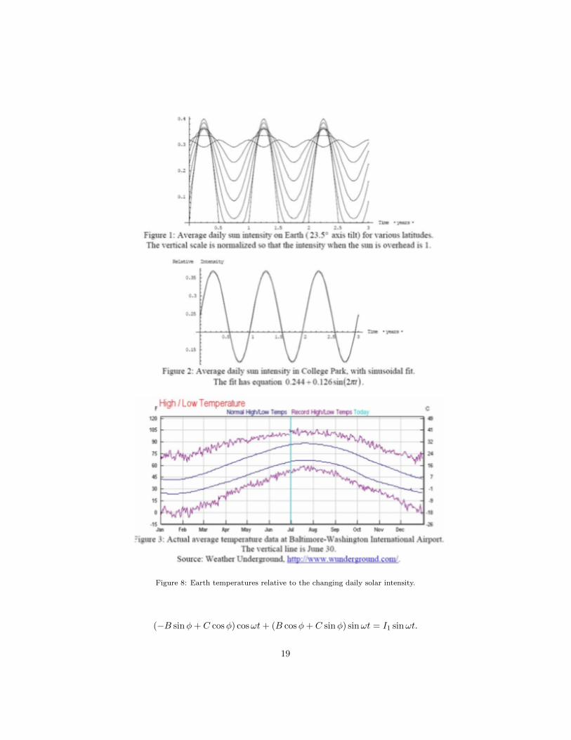
Figure 8: Earth temperatures relative to the changing daily solar intensity.

(−B sinφ+ C cosφ) cosωt+ (B cosφ+ C sinφ) sinωt = I1 sinωt.

19

As this occurs for all t, we equate the coefficients of the sines and cosines of ωt,and get

−B sinφ+ C cosφ = 0, B cosφ+ C sinφ = I1,

and thus,385

B = I1 cosφ, C = I1 sinφ.

NowB/A = I1 cosφ/I0 = 4σT 3

0 T1/σT40 = 4T1/T0,

we find a curious relation to the phase difference to the peak temperature giventhe solar intensity cycle shown in Figure 3:

cosφ = 4T1T0/I1I0.

Note that from the Figure, I1/I0 = 0.126/0.244 = 0.516, and so the assump-tion T1 T0 may not be quite valid in using the binomial approximation inthe quartic expansion above. More detail can be done numerically to solve this390

nonlinear driven differential equation to get more precise results. For exam-ple, with the data in the Figure and the analysis done here, we could plot thetemperature difference from winter to summer:

∆T = 2T1 =T0I12I0

cosφ = (73.1 K) cos(tπ

6 month).

According to the data the peak temperature occurs about 1 month aftersolstice, so that the summer-winter temperature difference peak is then about395

62 C, about 2.5 times the average temperature data for the globe.

5. Electric circuit equivalents of climate change and experimental re-sults

Now let us turn to global warming specifically. We look at a more anthro-pomorphic reason for the causes of global warming as a certain ’heat pump’,400

and model it as an RC network and make the details more specific and com-prehensive to the model as we proceed. We claim that electrical and humanactivity causes a significant effect to global warming compared to greenhousegases. Figure 4 shows the CO2 levels in our atmosphere as an exponentiallyramping set of rising and decaying exponentials as we will see later.405

As seen in the last example, it takes awhile after solar heating for the Earthto warm up, as well as it takes time to reach peak temperatures after a summersolstice. Thus there is a phase lag just like in RC alternating current circuits.Considering first a charging capacitor, it charges with a time constant (timeto cool to 1/e of the initial amplitude) of τ = RC, whereas from the solution410

to Newton’s law of cooling in two Sections ago, we find a time constant ofτ = mc/hA. Now we can make a direct analogy to RC circuits then: the

20

Figure 9: Atmospheric rise in CO2 levels over a couple generations [5].

greater the heat conductivity h, the lower the resistance to heat transfer, andthe larger the cross-sectional area A, the smaller the resistance. Thus 1/hAacts as the circuits resistance. Also, the larger the mass and heat capacity of415

the atmosphere, the more heat it can hold as charge can be held in a largercapacitor, and so mc acts as the capacitance of the circuit. From then the basicphasor diagram for the RC circuit, the phase difference for the voltage (i.e.temperature) across the capacitor can then be found easily. I summarize:

1/hA ⇐⇒ R, mc ⇐⇒ C, φ = tan−11

ωRC.

In real global warming models both land and the oceans and the atmosphere420

have different values of R and C, and they all exchange heat/’discharge’ intoone another. Thus an infinite chain network of cascading RC components isneeded...

To model anthropomorphic effects on global warming, let us apply now asquare wave, that possibly slowly ramps up over time, to an RC circuit with425

an initially discharged capacitor. As the square wave turns on the capacitorcharges, then as it turns off it discharges, but does not have time to fully dis-charge/’cool’. Then it charges again and reaches a higher voltage/’temperature’,and continues to charge more and more. This is called a charge pump, or in theatmosphere analogy, a heat pump to model global warming. Note that eventu-430

ally the curve flattens out as it reaches equilibrium, the idea though is that eachcycle, whether it represents human activity over a day or a year or a generation,can show slow temperature increases over time. A basic experiment was doneas shown in the following Figures, exaggerated for visual purposes.

The temperature change in this model can be easily determined mathemat-435

ically as well. In the RC circuit the charge (proportional to electric potential)

21

across the capacitor represents the temperature of the mean atmosphere. Wecan represent a ’hot’ temperature of T0 of about 127C, which represents thepeak temperature of the moon in the sunlight, and a ’cold’ temperature of theouter space of about 0K. We assume a regular period of charging and discharg-440

ing (for now) of the capacitors of time t, with (possibly unequal, but equal fornow) charge and discharge time constants τ = RC, where the values of R andC change for land, ocean and atmosphere. After the first charge and dischargethe thermal battery will have temperatures

T1 = T0(1− e−t/τ ), and T ′1 = T1e−t/τ .

After charging again the next day or next cycle, the remaining ’charge’ accu-445

mulates and after the next pump cycle the temperature is

T2 = (T0 − T ′1)(1− e−t/τ ) + T ′1, and T ′2 = T2e−t/τ ,

and similarly T3 = (T0 − T ′2)(1− e−t/τ ) + T ′2, etc.To find the global temperature increase of the thermal battery/charge pump,

we then find

∆T (n cycles) = Tn − T1 =

= (T0 − Tn−1e−t/τ )(1− e−t/τ ) + Tn−1e−t/τ − T0(1− e−t/τ ) =

= Tn−1e−2t/τ ,

which gives a nice recurrence relation for the temperature increases. In fact on450

can find a nice pattern (ε ≡ e−t/τ ):

T2 − T1 = T1ε2, T3 − T1 = T2ε

2 = T1(1 + ε2)ε2,

T4 − T1 = T3ε2 = T1(1 + ε2 + ε4)ε2,

. . .

Tn − T1 = T1(1 + ε2 + ε4 + · · ·+ ε2(n−2))ε2.

Thus the predicted temperature change due to the (n) anthropomorphiccycles is given by:

∆T (n) = T1ε2(1− ε2n)

1− ε2= T0

ε2

1 + ε(1− ε2n).

Note that even after an infinite number of cycles the Earth will never warmto the peak temperature without atmosphere T0 like the moon, but only a455

fractional increase from the original T1 of order ε2. This is good news as thenhaving a cycle or two off of anthropogenic heating will greatly reduce this number

22

and make the effect of anthropomorphic global warming a factor of order ε4 forone day or heating cycle skipped as opposed to the ε2 observed here!

Now let us calculate some numbers... We have from [6] the following reported460

values for R and C values and the relaxation time constant τ for the Earth’sland, oceans, and atmosphere:

Table 1: Relaxation times and RC values for the Earth under square wave responses.

/// τ (month) R (K/W/m2) C (MJ/Km2)

Air 1.02 0.1 10.2Land 1.04 0.243 11.2Ocean 2.74 0.0221 326Global 1.69 0.058 168

Plugging in the data for a simple one day off of power a week (no days-in-row) we find ε2/(1 + ε) ≈ 60% of the usual temperature differential increasealready! That is by simply removing 4 of 30 anthropomorphic heat cycles, we465

reduce the temperature increase of the planet due to anthropogenic effects by40%! This makes up to 50% of the temperature increase of the globe as reportedin the prize winning paper [6] and so we have already reduced 20% of the IPCC’sclimate temperature change budget! This effect is even greatly augmented if wedid two days in-a-row of heat off twice a month, leading to a quartic power of470

ε: ε4/(1 + ε) ≈ 31%, which means a reduction of global temperature increasesdue to anthropomorphic effects of almost 70%, and hence a reduction in 35%to global temperature increases over many anthropomorphic cycles!

Figure 10: RC circuit of anthropomorphic heat pump in global warming.

23

Figure 11: Modified circuit modelling climate change with atmospheric window taken intoaccount [7].

6. The quantum case with discrete emission spectra

Our model assumes that the atmosphere emits as a blackbody, or an objectat uniform temperature that absorbs and emits perfectly at all wavelengths.This assumption fails on multiple counts, however. As the troposphere does nothave a uniform temperature, but rather exhibits temperatures ranging roughlyfrom 200 - 300 K. Furthermore, the atmosphere is clearly not a perfect absorberat all wavelengths; this is obvious in the visible part of the radiation spectrum,and is also true in some regions of the thermal infrared. Indeed, individualgreenhouses gases such as carbon dioxide and water vapour absorb and emitpreferentially at some wavelengths and less so at others, yielding characteristicemission levels zem(λ) and temperatures Tem(λ) which depend on wavelength λ.The key ingredient in building a more refined model of OLR is under- standingTem(λ), because then the OLR may be estimated using the spectrally resolvedPlanck density

B(λ, T ) =2hc2

λ51

exp(hc/kTλ)− 1

(in W/m2/sr/m) as475

OLR =

∫πB(λ, Tem(λ))dλ,

24

Figure 12: Squarewave generator as anthropomorphic pump using 555 timer.

Figure 13: Experimental setup and display of ’heating and cooling’.

where the factor of π comes from the integration over solid angle, so the OLRflux is in W/m2. We thus turn to the question of what sets the emission levelat a given λ, focusing on water vapour emission since water vapour absorbs andemits effectively across a much wider range of λ than any other greenhouse gas.

Consider an atmospheric column with water vapour molecules whose density480

25

Figure 14: Output of the experimental thermal heat pump.

Figure 15: AC circuit result of phase lag for smaller C and R circuit describing a smalleratmosphere planet.

ρv decreases exponentially with height, and let us consider the emission to space(i.e. the contribution to the OLR) from these molecules, as pictured in Fig. 4.The top two layers in Fig. 4 have little difficulty emitting to space because theirview is unobstructed, but the density of emitters in these layers is relatively low,so the emission will also be low. In the third layer, the molecules view of space485

is still unobstructed (just barely), and the density is higher, so emission to spaceis higher. For layers four and five there are plenty of emitters, but their view isalmost totally obstructed, so their emission to space is very low. Thus, emissionto space is maximized around a sweet spot where the absorbers/emitters abovehave not yet totally obstructed the view of space, but the density is high enough490

26

Figure 16: AC RC circuit with larger R and C values describing a heavier atmosphere planetshowing a greater phase lag with less heating.

Figure 17: Full equivalent climate circuit for global warming thermal battery with anthropo-morphic source.

for emission to be appreciable. This sweet spot will be our emission level.To formalize this we need the notion of optical depth, defined as

τλ(z) ≡ κ(λ)

∫ ∞z

ρvdz =Effective area of absorbers

Actual area of column.

Here κ(λ) is the effective cross-sectional area of water vapour molecules atwavelength λ per unit mass. Applying this to the cartoon in Fig. 3, we seethat above our sweet spot we have τλ < 1 (the ’optically thin’ regime) and495

below our sweet spot we have τλ > 1 (the ’optically thick’ regime), and thus

27

Figure 18: IR cooling through the atmospheric window.

our sweet spot occurs around τλ ≈ 1. For simplicity we further assume that allthe emission occurs at exactly τλ = 1; we refer to this as the unit optical depthapproximation, and with it in mind we define our emission height zem(λ) by therelation τλ(zem(λ)) < 1. This is where the radiation (in the appropriate optical500

window near 10 µm) can then leave the Earth’s atmosphere and then cool theEarth. Ref. [7] shows a detailed equivalent circuit that takes into account theatmospheric window and other heat transfers. It does not, however, include theeffect of anthropomorphic heating, such as a square wave source. This can bedone in future studies.505

Also, we can calculate the time it takes for warm air parcels to convect to thetop of the Earth’s troposphere. We consider the buoyancy of such a parcel ofair (everything with a prime on it denotes the parcel, the atmosphere is withouta prime on it) and find its acceleration

a′z =ρ− ρ′

ρ′g = − 1

ρ′∂p

∂z− g =

=T ′ − TT

g =T ′(p0/p

′)R/cP − T (p0/p)R/cP

T (p0/p)R/cPg =

γ − Γ

T0 − γzgz,

where for the parcel we have approximately, T ′(z) = T0 − Γz with Γ the dry510

adiabatic lapse rate, and for the atmosphere, T (z) ≈ T0 − γz with the envi-

28

ronmental lapse rate γ. A simple back of the envelope calculation gives anauto-convective lapse rate for which the atmosphere has an actual increasingdensity with height, ∂ρ/∂z > 0. To see the change in temperature with height,differentiate the ideal gas law:515

∂p

∂z= RT

∂ρ

∂z+Rρ

∂T

∂z,

where then ∂ρ/∂z > 0 implies that

1

RT(∂p

∂z= −ρg)− ρ

T

∂T

∂z> 0 → ∂T

∂z> −−ρg

Rρ= g/R = 34.2 K/km.

This is a large value which occurs only metres above the surface and at highsolar irradiance. This would be responsible for dust devils.

A simple calculation including drag for a few degrees temperature differenceleads to air parcel velocities of about 10-20 cm/s, and so it would take up to 28520

hours for an air parcel to reach the top of the troposphere at around 10 km tocool down and radiate as a blackbody. However, it may be able to radiate outinto the atmospheric window at lower altitudes before this, and so convectivecooling is of the same time scale as the anthropomorphic time scales. This isinteresting as our application is to turn off human heating on this same time525

scale.

7. Conclusions

A radiative-convective model of the Earth’s atmosphere was studied and itsclimate and energy balance examined with anthropomorphic effects taken intoaccount. An equivalent RC circuit model was derived and built for both sine530

wave and square wave sources to model climate change from solar and humanimpacts respectively. It was found by direct calculation that even a couple daysof power off a few months of the year limits the anthropomorphic effect to globalwarming exponentially.

Funding.535

“This research received no external funding”

Acknowledgments.

Many thanks to Jode Himann and Brad Fincaryk of Nemalux for advice andfinancial contributions. Brett Teeple would like to thank Valerie Barclay as wellfor comments, support and hospitality during this research.540

Conflicts of interest.

“The authors declare no conflict of interest.”

29

References

[1] ipcc, Epa global greenhouse gas emissions, https://globalwarmingsummit.com/2020/03/06/epa-global-greenhouse-gas-emissions/, online; Acessed:545

02 May 2020 (2014).URL https://www.ipcc.ch/report/ar5/wg3/

[2] GISTEMP Team, Giss surface temperature analysis (gistemp), version 4.nasa goddard institute for space studies., https://data.giss.nasa.gov/gistemp/, online; Acessed: 14 Apr 2020 (2020).550

[3] N. Lenssen, G. Schmidt, J. Hansen, M. Menne, A. Persin, R. Ruedy, D. Zyss,Improvements in the gistemp uncertainty model, J. Geophys. Res. Atmos.124 (12) (2019) 6307–6326. doi:10.1029/2018JD029522.

[4] N. Jeevanjee, The physics of climate change: simple models in climate sci-ence (2018). arXiv:1802.02695.555

[5] Climate Atlas of Canada, Climate change: The basics, https://

climateatlas.ca/climate-change-basics, online; Acessed: 30 Apr 2020(2018).

[6] J. Kauppinen, J. T. Heinonen, P. J. Malmi, Major portions in climatechange: Physical approach, International Review of Physics (I.R.E.PHY.)560

5 (5) (2011) 260–270.URL https://butler.cc.tut.fi/~trantala/opetus/files/FS-1550.Fysiikan.

seminaari/Fileita/J.Kauppinen-IREPHY-21Nov13.pdf

[7] H. I. Abdussamatov, A. I. Bogoyavlenskii, S. I. Khankov, Y. V. Lapovok,Modeling of the earth’s planetary heat balance with electrical circuit anal-565

ogy, Journal of Electromagnetic Analysis and Applications 02 (03) (2010)133–138. doi:10.4236/jemaa.2010.23020.URL https://doi.org/10.4236/jemaa.2010.23020

Further Reading

[1] D. Olbers, A gallery of simple models from climate physics, in: Stochastic570

Climate Models, Birkhauser Basel, 2001, pp. 3–63. doi:10.1007/978-3-

0348-8287-3_1.URL https://doi.org/10.1007/978-3-0348-8287-3_1

[2] P. Gierasch, R. Goody, An approximate calculation of radiative heatingand radiative equilibrium in the martian atmosphere, Planetary and Space575

Science 15 (10) (1967) 1465 – 1477. doi:https://doi.org/10.1016/0032-0633(67)90080-3.URL http://www.sciencedirect.com/science/article/pii/0032063367900803

30