new anti-jamming technique for gps and galileo receivers ... · new anti-jamming technique for gps...

Digital Signal Processing 16 (2006) 255–274

www.elsevier.com/locate/dsp

New anti-jamming technique for GPS andGALILEO receivers using adaptive FADP filter ✩

René Jr. Landry ∗, Pierre Boutin, Aurelian Constantinescu

Ecole de Technologie Supérieure, Montreal, QC H3C 1K3, Canada

Available online 8 August 2005

Abstract

Anti-jamming techniques to improve Global Positioning System (GPS) receiver’s robustness havebeen mainly developed in military applications. None of civilian techniques can procure sufficientrobustness against occasional or intentional jammers for civil GPS or GALILEO navigation re-ceivers. The amplitude domain processing (ADP) filtering is a technique based upon Capon worksand Neyman–Pearson theory. Several experiments concerning the ADP filtering have been consid-ered at the 3DETSNAV division of LACIME laboratory at Ecole de technologie supérieure (ETS),which have proved that the technique is reliable in order to eradicate powerful interference present inthe spread spectrum signal. However, the results show that the ADP filter has a real limitation whensubmitted to multiple interference scenarios. This paper shows that working in the frequency domainis more efficient because jamming signals added to a white Gaussian noise are easier to detect and toattenuate when represented in the frequency domain. The present paper gives mathematical elementsto complete the ADP theory in the frequency domain and presents the performances of an ADP in thefrequency domain (FADP) filter simulated in a Matlab Simulink environment. The filter is tested witha signal composed of a GPS C/A code (Gold sequence) drowned in a white Gaussian noise in pres-ence of one or several additional jammers (CWI, PWI, chirp). Several analyses are made upon thefilter output (signal to noise ratio, attenuation and power spectral density measurements). The resultsof the analysis show that the FADP can eradicate any kind of jammers of 20 dB above white Gaussiannoise. Correlation losses are measured; they are always under 0.5 dB. In the presence of one or twojammers, the performances of the FADP filter are better than those of the ADP filter. The FADP filter

✩ This work was supported by Natural Sciences and Engineering Research Council of Canada (NSERC) andFonds de Recherche sur la Nature et les Technologies (FCAR), along with CMC Electronics.

* Corresponding author. Fax: +1 514 396 8684.E-mail addresses: [email protected] (R.J. Landry), [email protected] (P. Boutin),

[email protected] (A. Constantinescu).

1051-2004/$ – see front matter © 2005 Elsevier Inc. All rights reserved.doi:10.1016/j.dsp.2005.04.015

256 R.J. Landry et al. / Digital Signal Processing 16 (2006) 255–274

can procure up to 20 dB processing gain with a maximum of 10 dB loss on SNR in worse jammingscenario. When the number of jammers increases, the performances remain convenient, whereas thetime-domain ADP filter becomes unable to be effective. In this paper, measurements are made witha number of jammers up to 15.© 2005 Elsevier Inc. All rights reserved.

Keywords: Adaptive filtering; CDMA anti-jamming; FADP; GPS; GALILEO; Simulink model

1. Introduction

Interference perturbations are of real concern for navigation systems. In the case oflow-power interference, anti-jam techniques are not always necessary because of spectralspreading, currently used in navigation systems, which will significantly attenuate the ef-fect of the jammers. But as soon as the power of the interference becomes more important,it is really useful to appeal to anti-jam techniques. Reference [1] gives a thorough study ofthe impact of jamming upon the capacity to detect the correct information with a GlobalPositioning System (GPS) receiver. Nevertheless, for the last twenty years, only few anti-jamming techniques were developed and implemented in GPS receivers in order to improvedata detection, except for military applications. Pre-correlation techniques, used before thestage of correlation, and post-correlation techniques used to improve the signal qualityafter the correlation stage can be distinguished. Several of them are evocated in [2].

Adaptive radiation chart antenna or fixed bandpass filtering can be considered in a re-ceiver before the correlation stage and may eradicate interference in far frequencies. Inmulti-standard receivers capable of receiving both GPS and GLObal NAvigation SatelliteSystem (GLONASS) signals, these techniques have some difficulties to detect jammerswhose frequency ranges are located between the GPS and GLONASS bands [3]. Otherpre-correlation techniques perform better results, like the use of an Automatic Gain Con-trol (AGC) with an adaptive Analog-to-Digital Converter (ADC), as presented in [4]. Onecan also mention digital techniques to reject interference in the frequency range of theuseful signal. They have the capability to be used at low cost with some minor modifi-cations and high efficiency. For example, adaptive spectral filtering consists in detectinginterference peaks in the signal spectrum and inserting at the exact location of the jammera stopband filter in order to attenuate the main power of the signal. Another example isthe Piranha filter, composed with a succession of adaptive notch filters which has been thetarget of a thorough study in [2,5].

Numerous techniques of post-correlation can also turn out to be useful to reject wideband Gaussian interference. The extended range correlator, presented in [6,7], maintainsthe code synchronization when tracking loop errors exceed values that can be tolerated bya standard correlator.

The amplitude domain processing (ADP) is based upon Capon works [8] and Neyman–Pearson theory [9]. This technique is fully adaptive and completely digital, allowing easyimplementation and high efficiency when jammers are located in the useful signal band.Unfortunately, very few papers are devoted to ADP filtering, which has proven to be areliable technique to eradicate powerful interference applied to a spread spectrum signal.

R.J. Landry et al. / Digital Signal Processing 16 (2006) 255–274 257

Fig. 1. Probability ratio concept, as referred to Neyman–Person and Capon works.

Reference [7] presents the results obtained in experiments on GPS P code, while Refs.[6,10,11] show simulation results on coarse/acquisition (C/A) GPS code. But the maindrawback of ADP filtering, as shown in [7,11] is the incapability to resist to scenarioshaving more than two simultaneous interferences.

Indeed, the ADP filter is really transparent to white Gaussian noise and to spread-spectrum navigation signals, by the same way allowing no deterioration of those signals.For example, when 3 or 4 different jammers are present in the spectrum, the resulting prob-ability density function (PDF) tends to a Gaussian characteristic. Consequently, a temporalADP filter becomes unable to differ multiple interference from Gaussian noise. Becausemost of interference is concentrated around a specific frequency range, the digital sig-nal processing in the frequency domain will be more efficient. Multiple interference willbe easier to detect because its spectrum is completely different from the white Gaussiannoise spectrum. Thus, after briefly reminding the principles of the ADP theory, this pa-per presents the differences between the spectral and the temporal ADP theories. Then thewhole structure of the ADP in the frequency domain (FADP) filter and the way it can beinserted in a standard GPS receiver will be presented in detail. The last part of this paper isaimed to expose the performances of the FADP filter and to compare the results with thoseobtained using a temporal ADP filter.

2. Theoretical basis of the FADP filter

The ADP technique is based upon Capon work [8] and statistical theory of Neyman–Pearson [9]. The main objective is to evaluate a probability ratio Λ(x), as function of thesamples of signal z(t), as statistically demonstrated in [12]. The presence or the absenceof the signal is determined by comparing this ratio to a decision threshold μN (see Fig. 1).

This method is optimum insofar as the error probability (the probability to detect a sig-nal whereas there is no signal or not to detect a signal whereas there is one) is minimized.First, the ADP filter theory will be elaborated. For more details, the reader could refer to[11,13,14]. Then, mathematical developments will be performed for the spectral represen-tation version of the ADP.

2.1. Elaboration of the ADP theory

The basis of this section can be found in [11], where some further elaborations havebeen considered. The same notation for the GPS signal application will be used in all this


Fig. 2. Optimized theoretical receiver in rectangular coordinates.

paper. The signal captured by the GPS receiver can be written as following:

z(t) = r(t, θ) + w(t), (1)

r(t, θ) = s(t) cos(ωt + θ), (2)

where r(t) is the modulated information, s(t) is the useful data, and w(t) is a whiteGaussian noise including potential interference. The detection problem is to decide be-tween z(t) = r(t, θ) + w(t) and z(t) = w(t), when the signal is absent.

After extraction of the base band quadrature components, the detection problem is todecide between xi = si cos θ + nxi ; yi = si sin θ + nyi and xi = nxi ; yi = nyi .

Let

fnn(x, y) =N∑

i=1

fnn(xi, yi)

be the input PDF of z(t). It can be shown that this function is equal to the noise PDF. Ac-cording to [13], the optimal probability ratio evocated in Fig. 1 can be written as following:

Λ(wx,wy) − 1 =[

1

N

N∑i=1

si∂fnn(xi, yi)/∂xi

fnn(xi, yi)

]2

+[

1

N

N∑i=1

si∂fnn(xi, yi)/∂yi

fnn(xi, yi)

]2

,

(3)

for a N -sampled complex signal, where x and y represent the real and imaginary partsof the signal z(t), wx and wy are the real and imaginary parts of the noise w(t) and sirepresents the samples of the signal s(t). This formula, represented in Fig. 2 (see [13]),can be easily used in a conventional receiver to achieve its optimum form. Equation (3) hasbeen obtained by making use of the small-signal assumption and by using an expansion offnn in a Taylor series around the values of the received data (xi, yi).

The drawback of the representation (3), while optimum, is that it is necessary to applya non-linear function upon the two channels I and Q (in phase and in quadrature, respec-tively), which doubles the required resources. Moreover, we need a perfect knowledge of


Fig. 3. Theoretical and simulated fn(r) of a white Gaussian noise (N = 2048).

the joint I and Q noise PDF and fast hardware to compute twice partial derivatives. Ac-cording to [14], it is possible to work in polar coordinates, because noise and signal carrierare not synchronized. Hence, the probability ratio (3) becomes

Λ(wx,wy) − 1 = 1

N2

N∑i=1

[sigr (ri)

]2[(x2

i + y2i )

r2i

]=

[1

N

N∑i=1

sigr (ri)

]2

, (4)

where

g(ri) = ∂/∂ri(fn(ri)/ri)

fn(ri)/ri= ∂

∂riln

fn(ri)

ri. (5)

With this amplitude representation a new non-linear function g(r) is introduced, wherefn(r) is the radial PDF of the useful signal amplitude r . In the absence of interference,fn(r) is a Gaussian distribution because a Gaussian noise has a circular symmetry and itsphase is uniformly distributed. The relation between both representations of PDF fn(r)

and fnn(x, y) (polar and rectangular representations, respectively) is:

fn(ri) = 2πrifnn(x, y). (6)

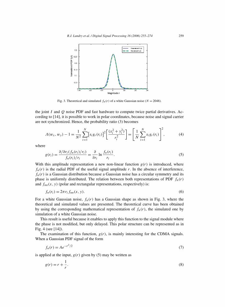
For a white Gaussian noise, fn(r) has a Gaussian shape as shown in Fig. 3, where thetheoretical and simulated values are presented. The theoretical curve has been obtainedby using the corresponding mathematical representation of fn(r), the simulated one bysimulation of a white Gaussian noise.

This result is useful because it enables to apply this function to the signal module wherethe phase is not modified, but only delayed. This polar structure can be represented as inFig. 4 (see [14]).

The examination of this function, g(r), is mainly interesting for the CDMA signals.When a Gaussian PDF signal of the form

fn(r) = Ae−r2/2 (7)

is applied at the input, g(r) given by (5) may be written as

g(r) = r + 1. (8)

r


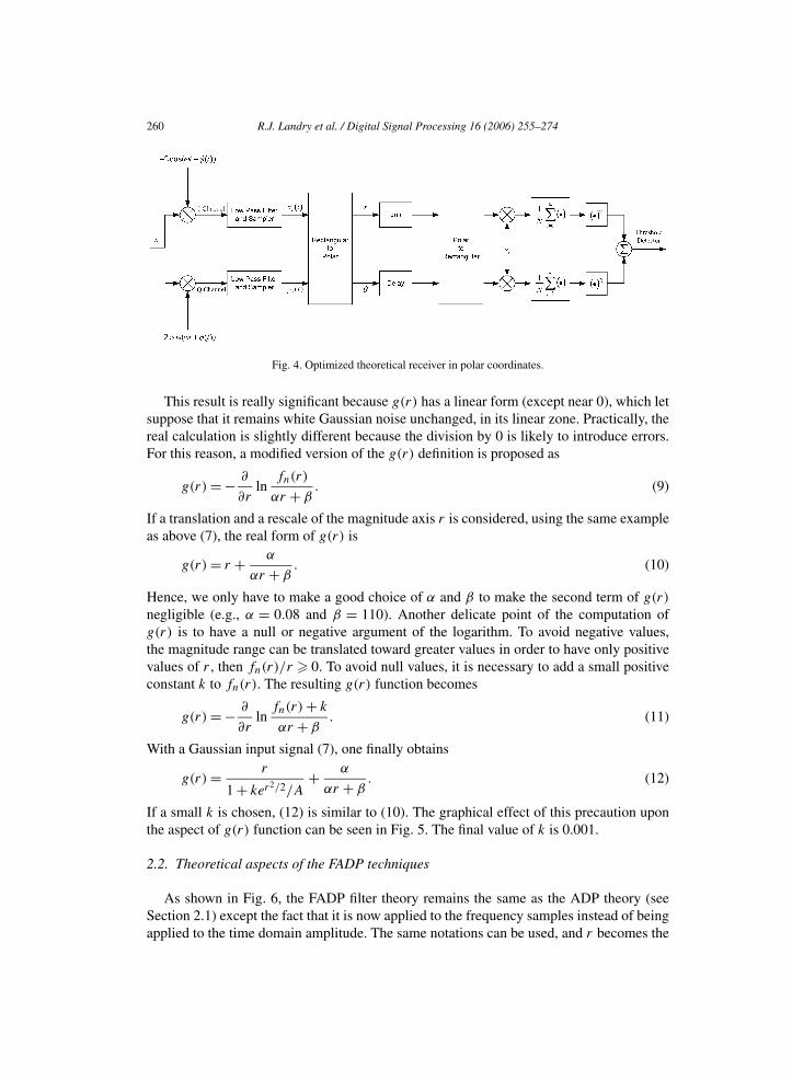
Fig. 4. Optimized theoretical receiver in polar coordinates.

This result is really significant because g(r) has a linear form (except near 0), which letsuppose that it remains white Gaussian noise unchanged, in its linear zone. Practically, thereal calculation is slightly different because the division by 0 is likely to introduce errors.For this reason, a modified version of the g(r) definition is proposed as

g(r) = − ∂

∂rln

fn(r)

αr + β. (9)

If a translation and a rescale of the magnitude axis r is considered, using the same exampleas above (7), the real form of g(r) is

g(r) = r + α

αr + β. (10)

Hence, we only have to make a good choice of α and β to make the second term of g(r)

negligible (e.g., α = 0.08 and β = 110). Another delicate point of the computation ofg(r) is to have a null or negative argument of the logarithm. To avoid negative values,the magnitude range can be translated toward greater values in order to have only positivevalues of r , then fn(r)/r � 0. To avoid null values, it is necessary to add a small positiveconstant k to fn(r). The resulting g(r) function becomes

g(r) = − ∂

∂rln

fn(r) + k

αr + β. (11)

With a Gaussian input signal (7), one finally obtains

g(r) = r

1 + ker2/2/A+ α

αr + β. (12)

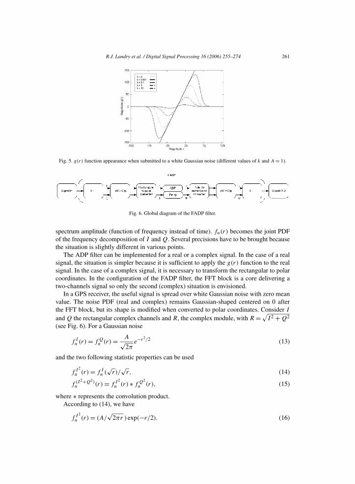
If a small k is chosen, (12) is similar to (10). The graphical effect of this precaution uponthe aspect of g(r) function can be seen in Fig. 5. The final value of k is 0.001.

2.2. Theoretical aspects of the FADP techniques

As shown in Fig. 6, the FADP filter theory remains the same as the ADP theory (seeSection 2.1) except the fact that it is now applied to the frequency samples instead of beingapplied to the time domain amplitude. The same notations can be used, and r becomes the


Fig. 5. g(r) function appearance when submitted to a white Gaussian noise (different values of k and A = 1).

Fig. 6. Global diagram of the FADP filter.

spectrum amplitude (function of frequency instead of time). fn(r) becomes the joint PDFof the frequency decomposition of I and Q. Several precisions have to be brought becausethe situation is slightly different in various points.

The ADP filter can be implemented for a real or a complex signal. In the case of a realsignal, the situation is simpler because it is sufficient to apply the g(r) function to the realsignal. In the case of a complex signal, it is necessary to transform the rectangular to polarcoordinates. In the configuration of the FADP filter, the FFT block is a core delivering atwo-channels signal so only the second (complex) situation is envisioned.

In a GPS receiver, the useful signal is spread over white Gaussian noise with zero meanvalue. The noise PDF (real and complex) remains Gaussian-shaped centered on 0 afterthe FFT block, but its shape is modified when converted to polar coordinates. Consider I

and Q the rectangular complex channels and R, the complex module, with R = √I 2 + Q2

(see Fig. 6). For a Gaussian noise

f In (r) = f Q

n (r) = A√2π

e−r2/2 (13)

and the two following statistic properties can be used

f I 2

n (r) = f In (

√r)/

√r, (14)

f (I 2+Q2)n (r) = f I 2

n (r) ∗ f Q2

n (r), (15)

where ∗ represents the convolution product.According to (14), we have

f I 2

n (r) = (A/√

2πr ) exp(−r/2). (16)


Fig. 7. Example of fn(r) appearance without (a) and with (b) the additional complex constant, C = 90(1 + i).

Then, using (15),

f (I 2+Q2)n (r) = [

(A/√

2πr ) exp(−r/2)]∗[

(A/√

2πr ) exp(−r/2)]. (17)

If we develop the convolution, the following integral must be evaluated:

f (I 2+Q2)n (u) =

u∫0

[(A/

√2πr) exp(−r/2)

][(A′/

√2π(u − r)

)exp(−(u − r)/2)

]dr.

(18)

We made the following variable change

x = r − u

2, (19)

and (18) becomes

f (I 2+Q2)n (u) = (AA′/2π) exp(−u/2) ln(1 + √

2) = K exp(−u/2), (20)

where K is a constant. With the use of (14), we have

f

√(I 2+Q2)

n (r) = Kr exp(−r2/2). (21)

Consequently, the development shows that a chi square-shaped PDF is obtained at theoutput of the FFT instead of a Gaussian distribution. The filter does not remain linearanymore with an input having a chi square-shaped PDF. Using (9) to compute the g(r)

function, the following formula is obtained with a chi square-shaped fn(r):

g(r) = − ∂

∂r

[−r2/2 + ln r + lnK − ln(αr + β)] = r − β

r(αr + β). (22)

The g(r) function in frequency domain diverges around 0. Therefore, it is useful to trans-form properly the FFT block output signal to obtain the original Gaussian form of fn(r).The solution adopted is to simply add a complex constant C to the output of the FFT block,which translates the spectral PDF on the spectral magnitude axis (see Fig. 7).


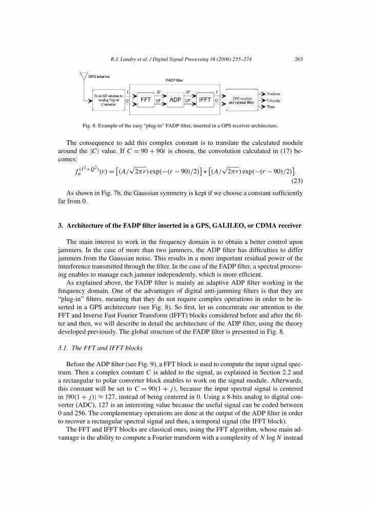
Fig. 8. Example of the easy “plug-in” FADP filter, inserted in a GPS receiver architecture.

The consequence to add this complex constant is to translate the calculated modulearound the |C| value. If C = 90 + 90i is chosen, the convolution calculated in (17) be-comes:

f (I 2+Q2)n (r) = [

(A/√

2πr) exp(−(r − 90)/2)] ∗ [

(A/√

2πr) exp(−(r − 90)/2)].

(23)

As shown in Fig. 7b, the Gaussian symmetry is kept if we choose a constant sufficientlyfar from 0.

3. Architecture of the FADP filter inserted in a GPS, GALILEO, or CDMA receiver

The main interest to work in the frequency domain is to obtain a better control uponjammers. In the case of more than two jammers, the ADP filter has difficulties to differjammers from the Gaussian noise. This results in a more important residual power of theinterference transmitted through the filter. In the case of the FADP filter, a spectral process-ing enables to manage each jammer independently, which is more efficient.

As explained above, the FADP filter is mainly an adaptive ADP filter working in thefrequency domain. One of the advantages of digital anti-jamming filters is that they are“plug-in” filters, meaning that they do not require complex operations in order to be in-serted in a GPS architecture (see Fig. 8). So first, let us concentrate our attention to theFFT and Inverse Fast Fourier Transform (IFFT) blocks considered before and after the fil-ter and then, we will describe in detail the architecture of the ADP filter, using the theorydeveloped previously. The global structure of the FADP filter is presented in Fig. 8.

3.1. The FFT and IFFT blocks

Before the ADP filter (see Fig. 9), a FFT block is used to compute the input signal spec-trum. Then a complex constant C is added to the signal, as explained in Section 2.2 anda rectangular to polar converter block enables to work on the signal module. Afterwards,this constant will be set to C = 90(1 + j), because the input spectral signal is centeredin |90(1 + j)| ≈ 127, instead of being centered in 0. Using a 8-bits analog to digital con-verter (ADC), 127 is an interesting value because the useful signal can be coded between0 and 256. The complementary operations are done at the output of the ADP filter in orderto recover a rectangular spectral signal and then, a temporal signal (the IFFT block).

The FFT and IFFT blocks are classical ones, using the FFT algorithm, whose main ad-vantage is the ability to compute a Fourier transform with a complexity of N logN instead


Fig. 9. Global implementation of the FADP filter.

Fig. 10. Global schematic view of the ADP filter.

of N2 for a classical discrete Fourier transform (DFT), where N is the size of the vec-tors submitted to the FFT and IFFT blocks. For the present application, we have chosenN = 256.

3.2. Structure of the ADP filter

The ADP filter used in the frequency domain remains close from the temporal ADP filterstructure, which is described in [10,11]. This section will bring some additional detailsconcerning the functioning of the filter in the frequency domain.

As shown in Fig. 10, there are four significant steps in the architecture implementationof an ADP filter. In the first step, a histogram fn(r) of the input signal is computed. Beforecalculating the g(r) function (using (5)), a filter block is inserted to smooth the real-timehistogram; this is the second step of the ADP architecture implementation. It contains aFinite Impulse Response (FIR) filter (smoothing filter), whose output is determined fromthe input using the following expression:


Fig. 11. Global testing environment for the FADP filter.

sout(i) = 0.125sin(i − 3) + 0.125sin(i − 2) + 0.125sin(i − 1) + 0.25sin(i)

+ 0.125sin(i + 1) + 0.125sin(i + 2) + 0.125sin(i + 3). (24)

As the ADP filter is adaptive, it is able to react immediately to a change of the inputsignal (e.g., brutal apparition of interference). But a severe change of the fn(r) functionwould entail a brutal change of the g(r) function and of the output signal. Consequently,the filter also contains a loop to avoid discontinuities in the case of important changes in theinput signal. This loop is introduced in the filter block. It is possible to make it more or lessstronger, by changing the gain percentage (the p value in Fig. 10). In order to acceleratethe convergence of the loop, it can be initialized with a Gaussian output function at thebeginning of the signal acquisition.

A small constant k (k = 0.001 has been chosen here) is added at the output of the fn(r)

function. This is made just before the calculation of g(r), which represents the third step ofthe ADP filter architecture implementation, in order to avoid computation problems (e.g.,ln(0)), as explained in Section 2.1. Then the g(r) function is computed and applied to theinput signal. The application of the g(r) function to the signal is the last step of the ADPblock implementation. The main difference between the FADP filter and the temporal ADPfilter is the following one: it is necessary to take care of the central value of the outputsignal, which is set to 127 instead of 0. The fn(r) and g(r) functions are also centeredaround 127 and the image of the g(r) function must be centered on 127, instead of 0,to create an output of the filter centered in 127. Thus, the g(r) function must be slightlychanged in the simulations, compared to [10,11], in order to shift the output signal.

4. Simulation of the FADP filter in a Simulink environment

In order to evaluate the ADP vs FADP filter performances, we need to build a testingsimulator (see Fig. 11). A GPS like signal is applied to an Automatic Gain Control (AGC),who normalizes the power of the signal. Next the signal is applied to the FADP filter forfurther performance analysis. First, we will deal with the signal source composition. Then,we will develop every means used to make performance measurements.

4.1. Signal generation

The input signal used in the simulator is a GPS C/A (Coarse Acquisition) code, createdwith Gold code generators G1 and G2 (see Fig. 12a). This Gold code is a periodic sequenceof 1023 chips evolving at a rate of 1.023 Mchips/s. Thus, the period of this pseudo-randomnoise sequence lasts 1 ms. The GPS satellites can use 37 orthogonal pseudo random se-quences and the simulator can select any of them. The phase selector in Fig. 12a willdetermine which satellite is chosen for the simulation. Figure 12b shows the frequency


Fig. 12. Synthesis of the C/A-code (a) and associated 5 MHz IF spectrum obtained with a sampling rate of20 Msamples/s (b).

Fig. 13. General structure of the simulator input signal.

spectrum of the Gold code centered at the Intermediate Frequency (IF) of 5 MHz (powerof 0 dB W). Additive White Gaussian Noise (AWGN) is added to the GPS signal alongwith several kinds of jammers. Simple gains (in dB) enable to calibrate the jammers andthe useful data JNR (Jammer-to-Noise Ratio) and SNR (Signal-to-Noise Ratio), respec-tively. Figure 13 shows a schematic view of the entire signal submitted to the simulator.

In order to consider the main jamming scenarios of the GPS signal, three types of jam-mers have been considered:

• Continuous wave interference (CWI). It is one of the most frequently encountered jam-ming signals, representing RF spikes, which could appear at any time in the spectrum.The spectral representation of the CWI jammer is presented in Fig. 20a.

• Pulsed wave interference (PWI). It corresponds mainly to signals emitted by RADARstations. The temporal and spectral representations of a PWI jammer are presented inFigs. 14 and 21a, respectively.

• Chirp interference. It is a sinusoidal interference including Doppler shift effect (varia-tion of the frequency in time). The spectrum of such a signal is spread on the frequencyrange covered by the signal due to the FFT time process. The temporal and spectralrepresentations of a chirp jammer are presented in Figs. 15 and 22a, respectively.


Fig. 14. Temporal representation of a PWI jamming signal with a 50% duty cycle (JNR = 20 dB, noise at 0 dB W).

Fig. 15. Temporal representation of a Chirp jamming signal (frequency between 5 and 7.5 MHz, JNR = 20 dB,noise at 0 dB W).

Several preliminary studies have been carried out upon the global source to verify theimpact of jammers on the GPS signal. GPS correlation losses (difference between corre-lation in absence and presence of a jamming signal) are measured, first in the presence ofa notch filter moving in the spectrum and finally in the presence of a CWI jammer. Theseresults are shown in Fig. 16 (sampling frequency of 20 Msamples/s). When a notch filteris centered in the main lobe of the GPS signal centered at 5 MHz, the correlation loss issignificant because of the GPS signal structure (see Fig. 16a). This is the main reason whya jammer whose frequency is located in the main lobe of the GPS signal (where 95% of itspower can be measured) affects the most GPS reception. Figure 16b emphasizes the linkexisting between JNR and correlation loss, which shows the impact generated by increas-ing the amplitude of the jamming signal.

4.2. Description of the analysis tools

To evaluate the FADP filter performances in simulation, the power ratio measurementsand the power spectral density (PSD) have been used. The definition of every ratio willbe reminded to clarify the following analysis. In the simulator, the input signal can beconsidered as in (1), with w(t) not necessarily a white Gaussian noise:

w(t) = n(t) + j (t), (25)


Fig. 16. (a) Correlation loss when GPS signal crosses a notch filter. (b) Correlation loss as function of the JNR ofa CWI.

Fig. 17. Computation of the real-time mean of crosscorrelation peak.

where n(t) is the white Gaussian noise considered above and j (t) is the sum of all jammingsignals. Using these notations, two ratios are computed, based on correlation measure-ments, as shown in [13]:

SNR = σ 2s /σ 2

n and JNR = σ 2j /σ 2

n , (26)

where σ 2s , σ 2

n , and σ 2j are the powers of s(t), n(t), and j (t), respectively (the variances of

the signal, noise and jammers).The main problem of the correlation peak computation lies in the fact that this mea-

surement needs a lot of signal samples (usually few C/A code periods) to have consistentcorrelation measurements. A sample rate of 20 Msamples/s was chosen in the simulator.A good measurement would need at least 20×1023 = 20,460 samples (which is equivalentto 1 ms period of the Gold sequence), resulting in a large processing time. Consequently,it was decided to organize the calculation differently, as shown in Fig. 17. The correlationpeak is computed with only 512 samples and a real-time mean block enables to obtain themean of an important number of peaks (100 or more). Moreover, it is possible to reini-tialize the mean block whenever. Thus, when the average is computed with more than 100correlation peaks, resulting measurement is surely reliable.

If a complex signal s composed of GPS data gps(t) and an important white Gaussiannoise n(t) are considered,

s(t) = gps(t) + n(t) (27)

the crosscorrelation between s and the GPS signal is written as

cl =N−1∑

sigpsi−k =N−1∑

(gpsi + ni)gpsi−k with −N � l � N, (28)
i=0 i=0


Fig. 18. Calculation of SNR and JNR ratios.

and

c0 =N−1∑k=0

gps2k +

N−1∑k=0

gpsknk. (29)

We can see that the crosscorrelation is finally the sum of the autocorrelation of the GPSsignal and the crosscorrelation between the GPS signal and the Gaussian noise. If we con-sider the correlation peak given by (29), obtained for l = 0, the first term is the GPS signalpower and the second one is mainly zero, because the crosscorrelation between noise andGPS data is a noise floor close to 0. Then the result of the crosscorrelation is close to theGPS signal power.

In the simulator, each signal power can be computed independently because crosscorre-lation terms are always negligible: useful data signal is really weak compared to the noisepower, so crosscorrelation between useful data and noise can be neglected. For the JNRcalculation, the jammer power is supposed to be weak at the output of the FADP filterso the crosscorrelation between jam and noise is negligible too. Consequently, the valuesobtained are reliable. If we are able to evaluate the GPS signal power and, with the samemethod, the noise and jammers powers, we are able to compute the output SNR and JNR.These data are obtained by computing the ratio between different correlation peaks, asshown in Fig. 18.

The SNR and JNR measurements give precious information concerning the quality ofthe output signal. With this information, we can compute processing gain and SNR lossdefined as

processing gain = JNRin/dB − JNRout/dB, (30)

SNR loss = SNRout/dB − SNRin/dB. (31)

The processing gain characterizes the ability to eradicate jammers and the correlation lossrepresents the ability to keep original useful signal unchanged.

In parallel, the power spectral density (PSD) is a discrete function of the frequency, asshown below:

P(mν0) =[

1

NTs

∣∣∣∣∣N−1∑i=0

x(iTs) exp(−2jπim/N)

∣∣∣∣∣]2

, (32)

where Ts is the sampling period, N is the number of signal samples and mν0 is the fre-quency, which is a multiple of a basis frequency ν0. In Fig. 19 are presented the graphicalrepresentations of the noise and useful signal PSD (power of 30 dB m). The PSD is com-


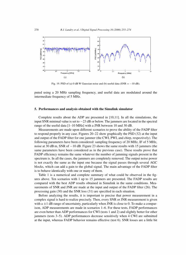
Fig. 19. PSD of (a) 0 dB W Gaussian noise and (b) useful data (SNR = −10 dB).

puted using a 20 MHz sampling frequency, and useful data are modulated around theintermediate frequency of 5 MHz.

5. Performances and analysis obtained with the Simulink simulator

Complete results about the ADP are presented in [10,11]. In all the simulations, theinput SNR minimal value is set to −23 dB or below. The jammers are located in the spectralrange of the useful data [1–10 MHz] with a JNR between 10 and 30 dB.

Measurements are made upon different scenarios to prove the ability of the FADP filterto respond properly in any case. Figures 20–22 show graphically the PSD (32) at the inputand output of the FADP filter for one jammer (the CWI, PWI, and chirp, respectively). Thefollowing parameters have been considered: sampling frequency of 20 MHz, IF of 5 MHz,noise at 30 dB m, SNR of −10 dB. Figure 23 shows the same results with 15 jammers (thesame parameters have been considered as in the previous case). These results prove thatFADP efficiency remains the same whatever the number of jamming signals present in thespectrum is. In all the cases, the jammers are completely removed. The output noise poweris not exactly the same as the input one because the signal passes through several AGCblocks, which can add a gain to the global signal. The main advantage of the FADP filteris to behave identically with one or many of them.

Table 1 is a numerical and complete summary of what could be observed in the fig-ures above. Ten scenarios with 1 up to 15 jammers are presented. The FADP results arecompared with the best ADP results obtained in Simulink in the same conditions. Mea-surements of SNR and JNR are made at the input and output of the FADP filter (26). Theprocessing gain (30) and the SNR loss (31) are specified in each situation.

Before analyzing the results, it is important to precise that power measurement in acomplex signal is hard to realize precisely. Then, every SNR or JNR measurement is givenwith a ±1 dB range of uncertainty, particularly when JNR is close to 0. To make a compar-ison, ADP measurements are made in scenarios 1–6. For these tests, FADP performancesare even better than ADP performances for CWI (tests 1 and 2) and slightly better for otherjammers (tests 3–5). ADP performances decrease sensitively when 4 CWI are submittedat the input, whereas FADP behavior remains effective (test 6). SNR losses are a little bit


Fig. 20. Input and output PSD with a CWI jammer (frequency of the jammer fj = 5 MHz, with JNR = 20 dB).

Fig. 21. Input and output PSD with a PWI jammer (frequency of the jammer fj = 5 MHz, with JNR = 20 dB).

Fig. 22. Input and output PSD with a chirp jamming signal (frequencies of the jammer fj = 5–7.5 MHz, withJNR = 20 dB).

more important in the case of jammers centered in the main lobe (tests 1 and 3). But withany kind of jammers, the output JNR is small enough for tests 1–6.

Tests 7–10 were not effective with the ADP filter (“−” in the table means that thetechniques used to measure ADP output SNR and JNR do not enable to obtain consistent


Fig. 23. Input and output PSD with 15 CWI centered in the main lobe of GPS signal (4.3 MHz � fj � 5.7 MHz,with a global JNR = 27 dB).

Table 1Comparative performances of ADP and FADP filter in several situations

Sort ofinterference

Inputs ADP outputs FADP outputs

SNRin(dB)

JNRin(dB)

SNRout(dB)

JNRout(dB)

SNRout(dB)

JNRout(dB)

Processing gain(dB)

SNR loss(dB)

1 CWI (4.7 MHz) −23 20 −27.0 8.0 −24.8 0.7 19.4 −1.81 CWI (2.1 MHz) −23 20 −23.4 8.0 −23.0 0.0 20.0 0.01 PWI (4.9 MHz) −23 20 −23.8 5.5 −23.9 5.3 15.0 −1.51 PWI (2.1 MHz) −23 20 −23.0 3.3 −23.0 3.5 16.5 0.01 chirp

(5000 points 2–6 MHz)−23 20 −23.6 2.3 −23.0 1.9 18.1 0.0

4 CWI −23 20 −25.3 9.0 −25.8 1.0 19.0 −2.82 CWI, 1 chirp,

and 1 PWI−23 20 – – −27.5 5.8 14.1 −4.6

5 CWI and 5 PWI −10 24 – – −17.5 11.5 12.5 −7.510 CWI −10 25 – – −17.2 9.5 15.5 −7.215 CWI −10 27 – – −19.4 9.0 17.0 −9.4

results) but FADP filter could still achieve good performances. The output JNR is moreimportant but the input JNR increases too. An increase of SNR loss is due to the impor-tant number of jammers, as most of them are located in the main lobe of the useful datasignal (between 4 and 6 MHz). This is the reason why the output useful data signal isaffected. Some tests have been already realized with the FADP filter inserted in a globalGPS receiver simulator. In the presence of the filter, the input JNR can be increased of20 dB W. Other anti-jamming techniques of post-correlation, like spectral dispreading en-able to manage a JNR of 10 dB at the output of the FADP filter.

Eventually, correlation loss has been measured in the absence of the jammer. A normal-ized input signal including a Gaussian noise (power of 30 dB m) and useful data drownedin the noise (SNR between −10 and −23 dB) is submitted at the input of the FADP fil-ter. The FADP output is also normalized. Values of useful data and signal crosscorrelationpeaks are measured before and after the filter. Correlation losses obtained are located be-tween 0 and −0.4 dB, as a function of the input SNR. This proves that the FADP filter letsthe useful data signal intact when it passes through the filter.


6. Conclusions

One of the main concerns with the use of the GPS and other positioning systems isthe ability to operate in all conditions and to maintain integrity in hostile environment. Inthis paper, we have shown that the FADP filtering could open new horizons in digital anti-jamming techniques. Digital processing in the FADP filter is pretty close to the ADP filter,no important changes being necessary except the addition of the FFT and IFFT blocksets.Then, measurement techniques have been the object of great thinking to be able to workas precise as possible in real conditions. In the presence of one or two jammers, the per-formances of the FADP filter are equivalent to those of the ADP filter. In the presence ofmore jammers, the FADP filter has shown to be more effective than the ADP one. Spectralprocessing enables to eradicate precisely all sorts of jammers, like PWI, CWI and chirp,whose frequencies are located in the main lobe of a GPS Gold sequence. JNR is reducedfrom at least 12 up to 20 dB when passing through the filter. Correlation loss, measured inabsence of jammers, is under 0.5 dB in any case.

Further investigations will be done with the FADP filter inserted in an entire GPS/GALILEO receiver Simulink model, in order to study its impact on the performances ofthe receiver. The simulation that we have evocated here with Simulink has been developedin order to be easily translated and implemented in a FPGA component. Real-time proofof concept demonstrator has been designed to be inserted in real GPS receiver in order tomeasure real performance of such a filter. Moreover, the great advantage of the FADP filteris its easy “plug-in” ability, enabling to insert it in any kind of CDMA receivers.

References

[1] A. Ndili, D.P. Enge, GPS receiver autonomous interference detection, in: IEEE Position, Location and Nav-igation Symposium—PLANS 98, Palm Spring, CA, 1998.

[2] R.J. Landry, Techniques de Robustesse aux Brouilleurs pour les Récepteurs GPS, Département d’Etudeset de Recherches en Automatique DERA/CERT et du Laboratoire Electronique et Physique, ENSAE,Toulouse, France, 1997, pp. 58–115.

[3] R.J. Landry, A. Renard, Analysis of potential interference sources and assessment of present solutions forGPS/GNSS receivers, in: Fourth St. Petersburg International Conference on Integrated Navigation Systems,St. Petersburg, 1997.

[4] F. Amoroso, Adaptive A/D converter to suppress CW interference in DSPN spread-spectrum communica-tions, IEEE Trans. Commun. COM-31 (10) (1983) 1117–1123.

[5] R.J. Landry, V. Calmetes, M. Bousquet, Impact of interference on a generic GPS receiver and assessment ofmitigation techniques, in: IEEE 5th International Symposium on Spread Spectrum Techniques and Applica-tions Proceedings, vol. 1, 1998, pp. 87–91.

[6] E. Balboni, J. Dowdle, J. Przyjemski, Advanced ECCM techniques for GPS processing, AGARD 488 (1988)3–12.

[7] J. Przyjemski, E. Balboni, J. Dowdle, B. Holsapple, GPS anti-jam enhancement techniques, in: Proceedingsof 49th Annual Meeting on Future Global Navigation and Guidance, Cambridge, MA, 1993.

[8] J. Capon, Optimum coincident procedures for detecting weak signals in noise, IEEE Trans. Inform. Theory(1960).

[9] V.R. Algazi, R.M. Lerner, Binary detection in white non-Gaussian noise, MIT Lincoln Laboratory Report,vol. DS-2138, 1964.

[10] R. AbiMoussa, R.J. Landry, Anti-jamming solution to narrowband CDMA interference problem, in: Cana-dian Conference on Electrical and Computer Engineering, vol. 2, 2000, pp. 1057–1062.


[11] R. AbiMoussa, Techniques de Robustesse aux Brouilleurs pour les Récepteurs GPS par un Traitement ADP,Master Memorandum, Ecole de technologie supérieure, Montreal, January 2001.

[12] P.Y. Arquès, Détection avec hypothèses non aléatoires, in: Décision en Traitement du Signal, Masson, 1982,pp. 154–160.

[13] D. Allinger, D. Fitzmartin, P. Konop, A. Tetewsky, P.V. Broekhoven, J. Veale, Theory of an adaptive non-linear spread-spectrum receiver for Gaussian or non-Gaussian interference, in: 12th Asilomar Conferenceon Signals, Systems and Computers, 1987.

[14] J.M. Malicorne, Approfondissement de la Technique ADP, ENSAE, Toulouse, France, September 1998.

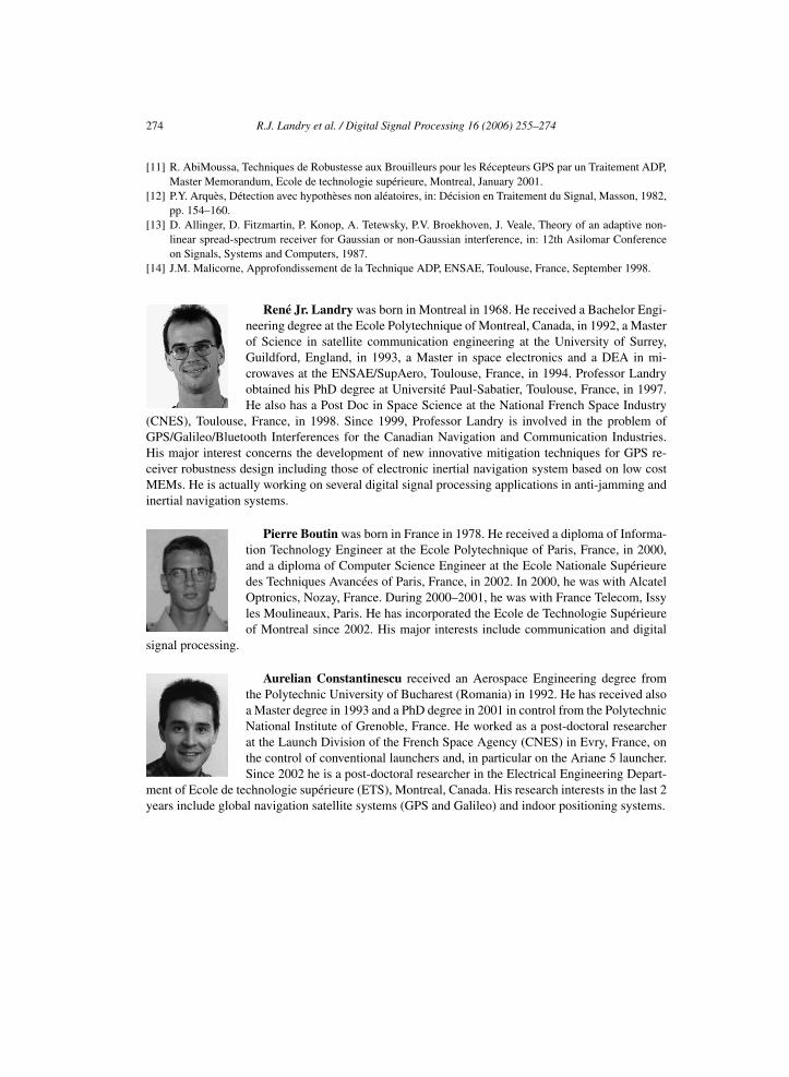
René Jr. Landry was born in Montreal in 1968. He received a Bachelor Engi-neering degree at the Ecole Polytechnique of Montreal, Canada, in 1992, a Masterof Science in satellite communication engineering at the University of Surrey,Guildford, England, in 1993, a Master in space electronics and a DEA in mi-crowaves at the ENSAE/SupAero, Toulouse, France, in 1994. Professor Landryobtained his PhD degree at Université Paul-Sabatier, Toulouse, France, in 1997.He also has a Post Doc in Space Science at the National French Space Industry

(CNES), Toulouse, France, in 1998. Since 1999, Professor Landry is involved in the problem ofGPS/Galileo/Bluetooth Interferences for the Canadian Navigation and Communication Industries.His major interest concerns the development of new innovative mitigation techniques for GPS re-ceiver robustness design including those of electronic inertial navigation system based on low costMEMs. He is actually working on several digital signal processing applications in anti-jamming andinertial navigation systems.

Pierre Boutin was born in France in 1978. He received a diploma of Informa-tion Technology Engineer at the Ecole Polytechnique of Paris, France, in 2000,and a diploma of Computer Science Engineer at the Ecole Nationale Supérieuredes Techniques Avancées of Paris, France, in 2002. In 2000, he was with AlcatelOptronics, Nozay, France. During 2000–2001, he was with France Telecom, Issyles Moulineaux, Paris. He has incorporated the Ecole de Technologie Supérieureof Montreal since 2002. His major interests include communication and digital

signal processing.

Aurelian Constantinescu received an Aerospace Engineering degree fromthe Polytechnic University of Bucharest (Romania) in 1992. He has received alsoa Master degree in 1993 and a PhD degree in 2001 in control from the PolytechnicNational Institute of Grenoble, France. He worked as a post-doctoral researcherat the Launch Division of the French Space Agency (CNES) in Evry, France, onthe control of conventional launchers and, in particular on the Ariane 5 launcher.Since 2002 he is a post-doctoral researcher in the Electrical Engineering Depart-

ment of Ecole de technologie supérieure (ETS), Montreal, Canada. His research interests in the last 2years include global navigation satellite systems (GPS and Galileo) and indoor positioning systems.

new anti-jamming technique for gps and galileo receivers ... · new anti-jamming technique for gps...

Documents